Extracting science from surveys of our Galaxy

James Binney

Oxford University

Outline

• The current challenge to stellar dynamics• How predictive is ¤CDM?• Why a model should yield a pdf, not a discrete

realisation• Why steady-state models are fundamental and

Jeans theorem is invaluable• Why observational errors require models to be

fitted in space of observables• Advantages of torus modelling• Some surprisingly useful worked examples

History

• Stellar dynamics started with Eddington, Jeans & others trying to understand early observations of the MW

• Chandra’s work in the field in the1940s was in this context

• From 1970s focus shifted to external galaxies and globular clusters

• In last 10 years focus has swung back to MW

Surveys

• Near-IR point-source catalogues– 2MASS, DENIS, UKIDS, VHS, ….

• Spectroscopic surveys– SDSS, RAVE, SEGUE, HERMES, APOGEE, VLT, WHT, …

• Astrometry– Hipparcos, UCAC-3, Pan-Starrs, Gaia, Jasmine, …

• Already have photometry of ~108 star, proper motions of ~107 stars, spectra of ~106 stars, trig parallaxes of ~105 stars

• By end of decade will have trig parallaxes for ~109 stars and spectra of 108 stars

• We are already data-rich & model-poor

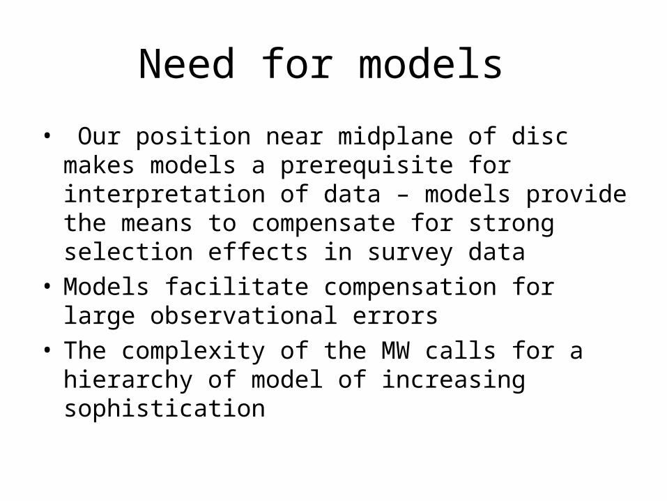
Need for models

• Our position near midplane of disc makes models a prerequisite for interpretation of data – models provide the means to compensate for strong selection effects in survey data

• Models facilitate compensation for large observational errors

• The complexity of the MW calls for a hierarchy of model of increasing sophistication

The ¤CDM paradigm

• ~30 yr of work on simulations of cosmological clustering of collisionless matter ! the ¤CDM paradigm

• Simulations very detailed & highly trustworthy• But a theory of the invisible!• All observations involve emag radiation & DM

emits none – although its gravitational field deflects light ! lensing

statistics

Baryon physics

• Dissipation by gas ! baryons dominate near bottom of potential wells

• The physics of baryons is horrifically complex (strong & emag interactions at least as important as gravity)

• Very small-scale phenomena (accretion discs, magnetic confinement, nucleosynthesis, blast waves) are important even for Galaxy-scale structure

• We hope that eventually an “effective theory” valid on Galaxy scales emerges from studies in small boxes

• Until then models from cosmological simulations are not based on sound physics but of “sub-grid physics” designed to make models agree with data

Philosophy

• We should not set out to “test ¤CDM paradigm” but to infer what’s out there

• Later we can ask if it’s consistent with ¤CDM

On pdfs & realisations

• Models from cosmological simulations are discrete realisations of some underlying probability density function (pdf) – we don’t expect to find a star exactly where the model has one

• The Galaxy is another discrete realisation• How to ask if 2 realisations consistent with same

(unknown) pdf?• Much better to formulate the model as a pdf – then can

ask if Galaxy is consistent with this pdf – or in what respects the Galaxy materially differs from it – by calculating likelihoods

• Hence reject N-body & similar models

Strategy

• The galaxy is not in perfect equilibrium• But we must start from equilibrium models:

– First target is ©(x), which will be an important ingredient of our final model

– Without the assumption of equilibrium, any distribution of stars in (x,v) is consistent with any ©(x)

– From ©(x) we can infer ½DM(x)– Can only infer ½DM(x) to the extent that the Galaxy is in

dynamical equilibrium• Non-equilibrium structure (spiral arms, tidal streams,..)

will show up as differences between best equilibrium model and the Galaxy

• The Galaxy is not axisymmetric, but it is sensible to start with axisymmetric models for related reasons

Jeans theorem

• Jeans (1915) pointed out that the distribution function (DF) of a steady-state Galaxy must be a function of integrals of motion f(I1,..)

• Jeans theorem simplifies our problem: 6d ! 3d• Already in 1915 observations implied that f must depend

on I3 in addition to E, Lz

• The Galaxy’s ©(x) will not admit an analytic form of I3(x,v) – must use numerical approximations

• Unfortunately, we need a large set of DFs: one for each physically distinguisable type of star:– f(E,Lz,I3,m,¿,Fe/H,®/Fe,..)– High-resolution spectroscopy further enlarges the space

inhabited by Galaxy models

Observational error

• The quantities of interest, E, Lz,… depend in complex ways on observables that may have large observational errors

• Observational errors ! correlated errors in E, Lz,..• For example error in distance s ! errors in vt = s¹ and

thus errors in E, L,…• Conclude: must match model to data in space of

observables u = (®,±,,¹®,¹±,vlos,log g,Fe/H,®/Fe,..) (recognising that log g, Fe/H, .. not raw observables)

• Calculate the likelihood of the data given a model by calculating for each star an integral that is in principle – P* = s dm d¿ dZ d6w f(w) iG(ui-ui(m,¿,Z,w),¾i)– where G(u,¾) is the normal distribution– in practice the integral can be greatly simplified

• Finally the model is adjusted to maximise ln(P*)

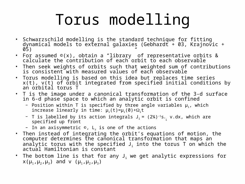
Torus modelling• Schwarzschild modelling is the standard technique for fitting dynamical

models to external galaxies (Gebhardt + 03, Krajnovic + 05)• For assumed ©(x), obtain a “library” of representative orbits & calculate the

contribution of each orbit to each observable• Then seek weights of orbits such that weighted sum of contributions is

consistent with measured values of each observable• Torus modelling is based on this idea but replaces time series x(t), v(t) of

orbit integrated from specified initial conditions by an orbital torus T• T is the image under a canonical transformation of the 3-d surface in 6-d

phase space to which an analytic orbit is confined– Position within T is specified by three angle variables µi, which increase linearly

in time: µi(t)=µi(0)+it– T is labelled by its action integrals Ji = (2¼)-1s°i

v.dx, which are specified up front– In an axisymmetric ©, Lz is one of the actions

• Then instead of integrating the orbit’s equations of motion, the computer determines the canonical transformation that maps an analytic torus with the specified Ji into the torus T on which the actual Hamiltonian is constant

• The bottom line is that for any Ji we get analytic expressions for x(µ1,µ2,µ3) and v (µ1,µ2,µ3)

Advantages of tori• Systematic exploration of phase space is easy• Action integrals:

– Are essentially unique– Are Adiabatic invariants– Have clear physical interpretation– Make integral (action) space a true representation of phase space:

d6w = (2¼)3d3J– Make choice of analytic DF easy

• Given T, for any x we can easily find the µi at which the star reaches x and determine the corresponding velocities v

• Knowledge of the µi of stars key to unravelling mergers (McMillan & Binney 2008)

• Angle-action variables (µ,J) are the key to Hamiltonian perturbation theory

• Kaasalainen (1995) showed that perturbation theory works wonderfully well when integrable H is provided by tori

Example: thin/thick interface

• Local stellar population can be broken down into– A “thick disc” of >10 Gyr old stars with high ®/Fe and

mostly low Fe/H– A “thin disc” with low ®/Fe and mostly quite high

Fe/H in which SFR has continued for ~ 10 Gyr at a slowly declining rate

• Thick-disc stars have quite large random velocities

• The random velocities of thin-disc stars increase steadily with age

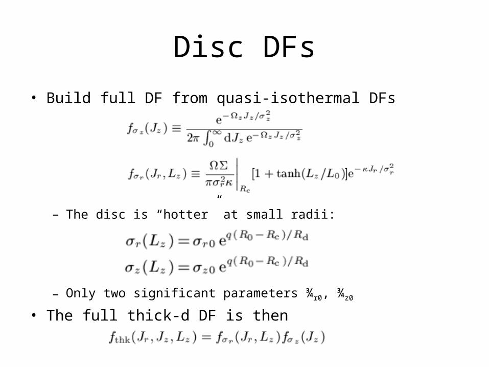
Disc DFs

• Build full DF from quasi-isothermal DFs

– The disc is “hotter” at small radii:

– Only two significant parameters ¾r0, ¾z0

• The full thick-d DF is then

Thin-disc DF

• Assume that all stars of a given age ¿ are described by an “isothermal” DF

• Assuming an exponentially declining SFR and ¾ » ¿¯, the thin-d DF is

• Adjusting the parameters we fit the data

Adiabatic approximation(Binney & McMillan 2010)

• To evaluate observables such as ½(R,z) or ¾z(R,z), we have to integrate over velocities

• This is most easily done if we can quickly evaluate Ji(x,v)

• Torus machine yields x(J,µ) & v(J,µ)• The integrals can be evaluated using

tori, but the “adiabatic approximation” greatly speeds evaluation

• Given (x,v) we define Ez= ½ vz

2+©(R,z) and estimate Jz = (2/¼)s0

zmax dz [2(Ez-©(R,z))]1/2

• Then we set L = |Lz| + Jz and estimate Jr = (1/¼)srp

radR [2(E-L2/2r2-Phi(R,0))]1/2

Further comparisons

• Conclude: adiabatic approx perfect in plane and very good for |z| < 2 kpc

DF for disc• Fit thin-d parameters to GCS stars

A successful predictionPreliminary RAVE data (Burnett 2010)

RAVE internal d.r.

Binney 10 model

Problem with V¯(arXiv0910.1512; Schoenrich + 2010)

• Shapes of U and V distributions related by dynamics

• If U right, persistent need to shift observed V distribution to right by ~6 km/s

• Problem would be resolved by increasing V¯

• Standard value obtained by extrapolating hVi(¾2) to ¾ = 0 (Dehnen & B 98)

• Underpinned by Stromberg’s eqn

V¯ (cont)• Actually hVi(B-V) and ¾(B-V) and

B-V related to metallicity as well as age

• On account of the radial decrease in Fe/H, Stromberg’s square bracket varies by 2 with colour

• Conclude V¯ = 12§2 km/s not 5.2§0.6 km/s

Schoenrich & B 2009

Schoenrich + 10

Stromberg [.]

Schoenrich & B 2009

Conclusions• There’s a huge and rapidly growing volume of survey data for MW• ¤CDM does not currently predict the structure of the MW• Key observables (,¹) are far removed from quantities of physical interest• Errors in s corrupt estimates of all physical quantities• Inversion of data to physical model ill-advised• Should fit model to data in (>6d) space of observables• To do this the model should deliver a pdf• Torus modelling can be considered a variant of Schwarzschild modelling in

which time series x(t) v(t) replaced by analytic 3d tori in 6d phase space• Advantageous to weight orbits by parameterised analytic DF rather than

varying weights of orbits independently• Adiabatic approximation yields very simple & useful expressions for J(x,v)

that are remarkably accurate for thin & thick discs• Early models have already

– correctly predicted ¾z(z)– revealed a subtle error in standard value of solar motion

• Examples given do not based on fits in space of observables – coming soon!

• We have a very long way to go before we are prepared for the Gaia catalogue

Example: vertical profilesMN 401, 2318 (2010)

• Vertical profile simply fitted

GCS

isothermal

prediction