extreme waves and tides.prn - oregon
TRANSCRIPT

Report to the
Oregon Department of Land
Conservation and Development
Salem, Oregon
ANALYSES OF EXTREME WAVES
AND WATER LEVELS ON THE PACIFIC
NORTHWEST COAST
PAUL D. KOMAR AND JONATHAN C. ALLAN
College of Oceanic & Atmospheric Sciences,Oregon State University, Corvallis, Oregon 97331, USA.
June 2000

ii
SUMMARY
Homes and other properties backing beaches are threatened by erosion during extreme events,when the runup of large storm waves on the beach is superimposed on exceptionally high tides.The objective of this report is to examine the potentially extreme waves and tides that can beexpected along the Pacific Northwest coast, ranging over time spans of 25 to 100 years.Reassessments of these processes are needed in that during recent winters the Northwest coasthas experienced both extreme waves and tides. In particular, during the 1998-99 La Niña, fourstorms generated deep-water significant wave heights that exceeded 10 meters, what had beenprojected in 1996 to represent the 100-year extreme event. During a storm on 2-4 March 1999,significant wave heights reached 14 meters, and measured tides were 1.75 m higher thanpredicted, mainly due to the associated storm surge.
This report begins with a re-analysis of the Northwest wave climate, the objective being to provideup-dated projections of the most extreme storm wave heights and periods. Analyses of wave dataderived from four ocean buoys off the Northwest coast, installed by the National Data Buoy Centerof NOAA, indicate that the revised 100-year deep-water significant wave height should be on theorder of 16 meters. However, the projection of future extreme-wave conditions is uncertain due tothe discovery that during the past 25 years of buoy measurements, wave heights off the Northwestcoast have progressively increased; for example, the buoy offshore from Washington documents arate of increase of 0.168 m/yr for the largest storm waves of the year, representing an increase inwave heights by 4.2 meters in 25 years. In that the climate factors which produced this increasehave not been clearly identified, it is not possible at present to predict whether this increase willcontinue and thereby affect the projections of the 25- through 100-year extreme wave heights.
Improvements in the predictions of extreme tides also have been accomplished through analysesof measured water levels that occurred during the major storms of the 1997-98 El Niño and 1998-99 La Niña. As in previous El Niños, it was found that the monthly mean water levels were raisedby 50 to 60 cm due to warmer ocean water temperatures and strong ocean currents. Analyses ofindividual storms demonstrated that the accompanying storm surges commonly elevated waterlevels by an additional 50 to 70 cm during the one to two days duration of the storm, while theextreme March 1999 storm generated a storm surge of 150 cm, which raised the measured tideabout 175 cm above the predicted tide due to the superposition of the storm surge above themonthly-mean water level.
This report ends with a discussion of how these multiple processes can be combined inapplications to evaluate potential water levels on beaches, to obtain predictions of the 25- to 100-year maximum levels achieved by the water due to the superposition of the runup of storm waveson top of exceptionally high tides. This is explored through analyses of three scenarios: (1) Anormal (non El Niño) winter, with the occurrence of a 100-year storm; (2) An El Niño wintercharacterized by high monthly-mean water levels that enhance the tides, but with the probability ofreduced storms; and (3) A “worst case” situation when a major storm occurs during an El Niñowhen there are elevated tides. Scenario #1 predicts a total water level of 7.3 meters NGVD29,mainly due to the high wave runup of the 100-year storm and the generation of a 1.75-meter stormsurge. In contrast, the El Niño scenario #2 yields a total water elevation of 5.9 meters NGVD29,less than scenario #1 because the elevated monthly mean water levels and measured tides of anEl Niño are not as great as the wave runup and storm surge contributions of a 100-year storm inscenario #1. This contrast demonstrates that beach and property erosion during an El Niño are notparticularly caused by extreme total water levels, but are due to “hot spot” erosion north ofheadlands and tidal inlets caused by the northward transport of beach sand within the littoral cells.Although the occurrence of a near 100-year storm is less likely during an El Niño year due to thesoutherly tracks of the storm systems, such an event cannot be entirely ruled out, and the “worstcase” scenario #3 represents that condition. However, the total water level of scenario #3 is onlyabout 30 cm higher than scenario #1. In spite of that small difference, management planning forscenarios #1 and #3 differ in that #3 includes the hot-spot erosion impacts associated with an ElNiño as well as the extreme wave runup and storm surge of a major storm, the factors important toscenario #1. All three scenarios predict the potential of significantly greater erosion impacts along
iii
the Northwest coast than were assessed in 1996, prior to the major 1997-98 El Niño and 1998-99La Niña winters.
In order to improve predictions of extreme events on the Northwest coast that may lead to majorerosion impacts, a better understanding is required of how the climate regime over the NorthPacific controls the strengths of storms and the waves they generate. Only with such anunderstanding can we predict whether the increases in wave heights and periods that haveoccurred during the past 25 years will increase during the next 25 to 100 years, and fully establishhow factors such as the occurrence of an El Niño or La Niña govern the wave conditions duringany particular year.

1
INTRODUCTIONThe most hazardous conditions occur in the coastal zone during extreme events, when large stormwaves are superimposed on exceptionally high tides. This is particularly true for homes and otherproperties backing beaches, where the elevated tide places the mean shoreline high up on thebeach, and the runup of the storm waves above that shore position reaches and erodes coastaldunes and sea cliffs, undermining the homes. Such a model for the analysis of coastal erosion hasbeen developed by Ruggiero et al. (1996, in press), with the primary focus being on applicationsalong the Pacific Northwest coast (PNW), Oregon and Washington. Analyses of extreme wavesand tides are important in other applications, such as in the engineering design of harbor jettiesand shore-protection structures.
The objective of this report is to examine the potentially extreme waves and tides that can beexpected along the PNW coast, ranging over times spans of 25 to 100 years. Reassessments ofthese processes are needed in that during recent winters the PNW coast has experienced bothextreme waves and tides. Those occurrences came during the El Niño winter of 1997-98 and LaNiña winter of 1998-99, suggesting that the severe storms may have been related to those globalclimate events. The need for revised estimates of extreme wave conditions is apparent in thatbased on wave measurements up through 1996, we had projected that the 100-year storm wouldgenerate a deep-water significant wave height of about 10 meters. That height was exceeded byone storm during the 1997-98 El Niño, while four 100-year storms occurred during the 1998-99 LaNiña, with one storm on 2-4 March 1999 having generated deep-water significant wave heights of14 to 15 meters.
This report begins with a re-analysis of the PNW wave climate, with the objective being to provideup-dated projections of the most extreme storm wave heights and periods. The report then turns toanalyses of extreme tidal elevations, a complex problem in that this depends on multipleatmospheric and oceanic processes that cause measured tides to reach substantially higher thanthe predicted tides. For example, the highest monthly mean water levels are known to occurduring El Niños, due to multiple causes including warmer offshore water temperatures and strongernorthward-flowing currents along the coast. But superimposed on the elevated monthly-meanwater level is the storm surge associated with an individual storm event, which may last for onlyone to two days. When one considers the several combined processes, it is difficult to predict theexpected extreme 25- to 100-year tidal elevations. This report ends with a discussion of how thesemultiple processes can be combined in applications to evaluate potential water levels on beaches,the 25- to 100-year maximum levels achieved by the water due the superposition of the runup ofstorm waves on top of exceptionally high tides.
THE PACIFIC NORTHWEST WAVE CLIMATEWave data for the PNW are available for nearly 45 years, if one includes the hindcast assessmentsundertaken by the Wave Information Study of the U.S. Army Corps of Engineers, which coveredthe years 1956 through 1975 (Hemsley and Brooks, 1989). However, in a comparison with directmeasurements of wave heights and periods that overlapped with the last few years of WIShindcasts, Tillotson and Komar (1997) found that the WIS values were systematically higher thanthe measured values, by 30 to 60%, so it was recommended that the WIS data not be used inapplications.
The earliest source of direct measurements of waves along the Northwest coast was themicroseismometer system of Oregon State University, which has been in operation since 1971 atthe Marine Science Center in Newport. That system is based on the theoretical analysis ofLonguet-Higgins (1950), which relates the generation of microseisms to the pressure field on theocean floor produced by standing waves that result from the interaction of incident waves and theirreflection from the coast. Based on this theory of microseism generation where the amplitudes andperiods of the microseisms are related to the heights and periods of the ocean waves, the Newportmicroseismometer was placed in operation in May 1971 to monitor the ocean wave conditions on adaily basis (Zopf et al., 1976). This required that the microseismometer record be calibrated
2
against the actual ocean waves, which was accomplished initially using visual observations ofwave heights and periods, and then with records from a pressure sensor located in 20-meters waterdepth offshore from Newport. The resulting calibrated wave heights derived from themicroseismometer showed good agreement with the heights measured visually and with thepressure sensor, yielding a correlation coefficient R2 = 0.76 and a standard error of 0.49 meters(Zopf et al., 1976). In a more extensive comparison, made possible by the installation of offshorebuoys, Tillotson and Komar (1997) confirmed that the Newport microseismometer provides goodassessments of significant wave heights, but poor results for wave periods.
The first buoys installed off the PNW coast to obtain long-term measurements of wave conditionswere placed by the National Data Buoy Center (NDBC) of NOAA in 1975 and 1976, respectivelywestward from the Oregon and Washington coasts. Those buoys are located in the deep-oceanbasin, about 500 to 600 km offshore, and provide the longest record of measurements derivedfrom buoys of PNW wave conditions. Beginning in the 1980s, buoys were also installed closer tothe coast, over the continental shelf, in deep to intermediate water depths. In 1981 buoys wereplaced offshore from Bandon on the south coast of Oregon, and offshore from Grays Harbor,Washington, by the Coastal Data Information Program (CDIP) of the Scripps Institution ofOceanography (Seymour et al., 1985). In 1983, CDIP also installed directional arrays in shallowwater (11-meters depth) off the Oregon and Washington coasts, to provide inshore data anddirections of wave approach to the shore. Additional buoys were placed by NDBC over thecontinental shelf, beginning in 1987, to the west of Newport and offshore from the Columbia River.
The several NDBC and CDIP buoys located over the continental shelf have been analyzed byprevious investigations (Tillotson and Komar, 1997; Ruggiero et al., 1996, in press; Komar et al.,1999). However, it is difficult to define the Northwest wave climate based on data from the inshoreNDBC buoys, due in part to the short lengths of the records (13 years), but in particular becausethere are numerous gaps of missing data. The CDIP buoys, installed in 1981, were withdrawn fromservice after 15 years of data collection, unfortunately just prior to the recent major El Niño and LaNiña winters when the wave conditions were exceptional. Because of such limitations in the datafrom buoys on the continental shelf closer to the coast, our analyses presented here have had torely almost entirely on the NDBC buoys #46005 (Washington) and #46002 (Oregon), Figure 1,located further offshore in the deep-ocean basin. We will only utilize data from the inshore buoysto confirm the evaluated extreme-wave conditions, the 10- through 100-year events, and thenmainly to resolve apparent discrepancies between our results and those presented earlier byTillotson and Komar (1997) and Ruggiero et al. (1996).
Allan and Komar (2000, in press) have analyzed the two NDBC buoys offshore from theWashington and Oregon coasts, along with buoys off the coasts of California and Alaska, Figure 1,in order to fully define the wave climate of the eastern North Pacific. Figure 2A gives the monthlymean significant wave heights and periods derived from the buoys, showing that on average thewave heights are comparable off the PNW to those in the Gulf of Alaska, and are on averageabout 1 meter higher than those off the coast of California. In the north the monthly-averagedsignificant wave heights reach their highest levels in November through January, on the order of3.6 to 3.8 meters. It is seen in Figure 2B that the wave periods are longest in the south, reachingon average to nearly 14 sec at the Point Arguello buoy, decreasing progressively to the north sothat on average they reach to only 11 sec in the Gulf of Alaska; in the Pacific Northwest the waveperiods during the winter average just over 12 sec.

3
Figure 1 Locations of the NDBC wave buoys in the North Pacific,analyzed by Allan and Komar (2000) to determine the wave climate.
Figure 2 Seasonal variability of monthly-averaged wave heights andperiods for the six buoys shown in Figure 1.
Wav
e H
eigh
t (m
)W
ave
Per
iod
(s)
Month
1.0
2.0
3.0
4.0A) Seasonal variation of the average monthly significant wave height
B) Seasonal variation of the average peak wave period
8.0May
9.0
10.0
11.0
12.0
13.0
Jun Jul Aug Sep Oct Nov Dec Jan Feb Mar Apr
4600146005
46002
4601446012
46023
#46001 - Gulf of Alaska
#46002 - Oregon
N#46014 - Pt. Arena
#46012 - Half Moon Bay
#46023 - Pt. Arguello
-150 -140 -130
40
50
-120
60
#46005 - WashingtonToke Point
Newport
Wave buoy
Tide gauge

4
Of special interest are the heights of the largest storm waves, graphed in Figure 3 for the series ofbuoys, arranged by latitude. In that the strongest storms and highest waves occur during the wintermonths, the results presented in Figure 3 focus on the wave conditions during October throughMarch. The lower curve (open squares) gives averages of the largest annual waves measured bythe buoys, averaged over the span of operation of each buoy. The upper curve (dark triangles)gives the maximum significant wave heights found within the entire record of the buoy. This lattergraph shows that off the PNW coast and in the Gulf of Alaska, the largest waves measured by thebuoys since they began to operate in the early to mid-1970s reached 14 to 15-meters deep-watersignificant wave heights. This provides an initial assessment of the most extreme wave conditionsexpected along the Northwest coast.
Figure 3 Latitude variations in winter wave heights measured by the sixNDBC buoys, Figure 1, evaluated as averages of the highest wavesexperienced each month during the winter (October through March), andas the largest waves measured during the operational life time of thebuoy.
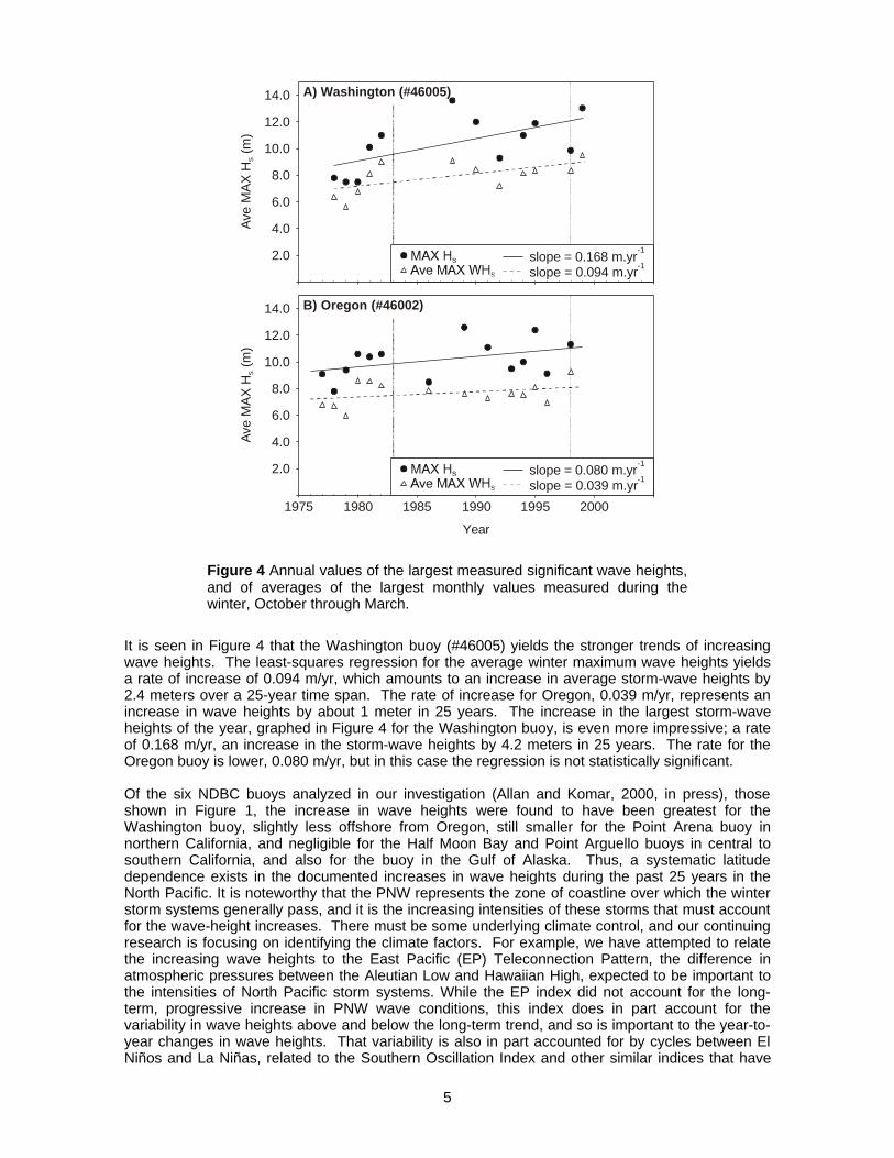
It has been found that wave heights off the PNW coast have been progressively increasing duringthe 25-year records provided by the NDBC buoys (Allan and Komar, 2000, in press). This increaseis shown in Figure 4 for the Washington (#46005) and Oregon (#46002) buoys, plots of the annualaverages of the highest wave heights measured during each of the winter months, again defined asOctober through March, and as the individual largest significant wave height generated by a stormduring that particular year. Upward trends are apparent in all of the graphs, the steeper the line thegreater the increase in wave heights during the 25-years of wave records. Although the recordsfrom the buoys on the continental shelf are shorter and more fragmentary due to missing data, theysubstantiate these trends of increasing wave heights documented by the offshore buoys.
Ave Wave Height (Winter)
Ave Wave Height (Year)
Max Wave Height (all records)Ave Max Wave Height (Winter)
Wav
e H
eigh
t (m
)
A) Latitude variation in the average significant wave height
B) Latitude variation in the average maximum significant wave height
46001 46005 46002 46014 46012 46023
NDBC Wave Buoy
1.5
2.0
2.5
3.0
3.5
4.0
14.0
12.0
10.0
8.0
6.0
4.0
5
Figure 4 Annual values of the largest measured significant wave heights,and of averages of the largest monthly values measured during thewinter, October through March.
It is seen in Figure 4 that the Washington buoy (#46005) yields the stronger trends of increasingwave heights. The least-squares regression for the average winter maximum wave heights yieldsa rate of increase of 0.094 m/yr, which amounts to an increase in average storm-wave heights by2.4 meters over a 25-year time span. The rate of increase for Oregon, 0.039 m/yr, represents anincrease in wave heights by about 1 meter in 25 years. The increase in the largest storm-waveheights of the year, graphed in Figure 4 for the Washington buoy, is even more impressive; a rateof 0.168 m/yr, an increase in the storm-wave heights by 4.2 meters in 25 years. The rate for theOregon buoy is lower, 0.080 m/yr, but in this case the regression is not statistically significant.
Of the six NDBC buoys analyzed in our investigation (Allan and Komar, 2000, in press), thoseshown in Figure 1, the increase in wave heights were found to have been greatest for theWashington buoy, slightly less offshore from Oregon, still smaller for the Point Arena buoy innorthern California, and negligible for the Half Moon Bay and Point Arguello buoys in central tosouthern California, and also for the buoy in the Gulf of Alaska. Thus, a systematic latitudedependence exists in the documented increases in wave heights during the past 25 years in theNorth Pacific. It is noteworthy that the PNW represents the zone of coastline over which the winterstorm systems generally pass, and it is the increasing intensities of these storms that must accountfor the wave-height increases. There must be some underlying climate control, and our continuingresearch is focusing on identifying the climate factors. For example, we have attempted to relatethe increasing wave heights to the East Pacific (EP) Teleconnection Pattern, the difference inatmospheric pressures between the Aleutian Low and Hawaiian High, expected to be important tothe intensities of North Pacific storm systems. While the EP index did not account for the long-term, progressive increase in PNW wave conditions, this index does in part account for thevariability in wave heights above and below the long-term trend, and so is important to the year-to-year changes in wave heights. That variability is also in part accounted for by cycles between ElNiños and La Niñas, related to the Southern Oscillation Index and other similar indices that have
slope = 0.094 m.yr-1
slope = 0.168 m.yr-1
Ave
MA
X H
(m
)S
4.0
6.0
8.0
10.0
14.0
2.0
12.0
A) Washington (#46005)
Year
1975 1980 1985 1990 1995 2000
Ave
MA
X H
(m
)S
4.0
6.0
8.0
10.0
14.0
2.0
12.0
B) Oregon (#46002)
slope = 0.039 m.yr-1
slope = 0.080 m.yr-1
6
been devised to measure intensities of El Niños and La Niñas. Important in this climate cycle arechanges in the paths of the storms, wherein during an El Niño the storm systems follow moresoutherly courses and cross the coast of central California, bringing high wave conditions to centraland southern California (Seymour et al., 1984; Seymour, 1998; Komar, 1986; Komar et al., 1999).With the storms following a more southerly course, it was expected that wave conditions in thePNW would be reduced somewhat during an El Niño, but this did not prove to be the case duringthe 1997-98 El Niño when we experienced unusually intense storms and high wave conditions.The intensities of the storms and heights of waves reached unprecedented levels during the 1998-99 La Niña, during which four storms generated deep-water significant wave heights equal to orgreater than 10 meters, with the March 1999 storm generating 14-meter significant wave heights.During a La Niña the storm systems are again crossing over the Pacific Northwest, so one wouldexpect higher waves than experienced during an El Niño, but the climate factors important to theoccurrence of extreme waves during the 1998-99 La Niña have not been positively identified. Theunusually large waves and numbers of storms in recent years must in part be the result of the long-term increase documented in Figure 4, but the underlying cause still remains to be determined.
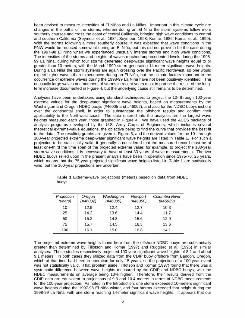
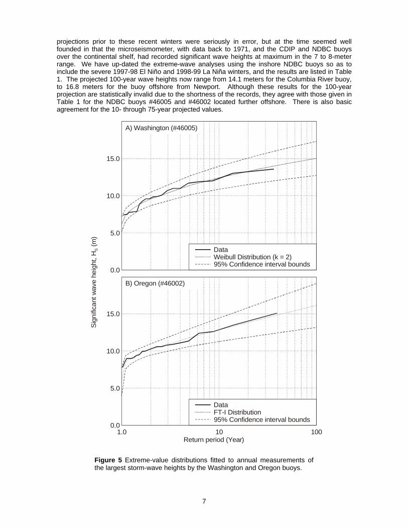
Analyses have been undertaken, using standard techniques, to project the 10- through 100-yearextreme values for the deep-water significant wave heights, based on measurements by theWashington and Oregon NDBC buoys (#46005 and #46002), and also for the NDBC buoys inshoreover the continental shelf, in order to substantiate the offshore results and confirm theirapplicability to the Northwest coast. The data entered into the analyses are the largest waveheights measured each year, those graphed in Figure 4. We have used the ACES package ofanalysis programs developed by the U.S. Army Corps of Engineers, which includes severaltheoretical extreme-value equations, the objective being to find the curve that provides the best fitto the data. The resulting graphs are given in Figure 5, and the derived values for the 10- through100-year projected extreme deep-water significant wave heights are listed in Table 1. For such aprojection to be statistically valid, it generally is considered that the measured record must be atleast one-third the time span of the projected extreme value; for example, to project the 100-yearstorm-wave conditions, it is necessary to have at least 33 years of wave measurements. The twoNDBC buoys relied upon in the present analysis have been in operation since 1975-76, 25 years,which means that the 75-year projected significant wave heights listed in Table 1 are statisticallyvalid, but the 100-year projections are uncertain.
Table 1 Extreme-wave projections (meters) based on data from NDBCbuoys.
The projected extreme wave heights found here from the offshore NDBC buoys are substantiallygreater than determined by Tillotson and Komar (1997) and Ruggiero et al. (1996) in similaranalyses. Those studies respectively projected 100-year significant wave heights of 8.2 and about9.1 meters. In both cases they utilized data from the CDIP buoy offshore from Bandon, Oregon,which at that time had been in operation for only 15 years, so the projection of a 100-year eventwas not statistically valid. That problem aside, Tillotson and Komar (1997) found that there was asystematic difference between wave heights measured by the CDIP and NDBC buoys, with theNDBC measurements on average being 13% higher. Therefore, their results derived from theCDIP data are equivalent to projections of 9.3 and 10.4 meters in terms of NDBC measurementsfor the 100-year projection. As noted in the Introduction, one storm exceeded 10-meters significantwave heights during the 1997-98 El Niño winter, and four storms exceeded that height during the1998-99 La Niña, with one storm reaching 14-meter significant wave heights. It appears that our
Projection(years)
Oregon(#46002)
Washington(#46005)
Newport(#46050)
Columbia River(#46029)
10 12.9 12.4 12.7 10.325 14.2 13.6 14.4 11.750 15.2 14.3 15.6 12.975 15.7 14.5 16.3 13.6
100 16.1 15.0 16.8 14.1
7
projections prior to these recent winters were seriously in error, but at the time seemed wellfounded in that the microseismometer, with data back to 1971, and the CDIP and NDBC buoysover the continental shelf, had recorded significant wave heights at maximum in the 7 to 8-meterrange. We have up-dated the extreme-wave analyses using the inshore NDBC buoys so as toinclude the severe 1997-98 El Niño and 1998-99 La Niña winters, and the results are listed in Table1. The projected 100-year wave heights now range from 14.1 meters for the Columbia River buoy,to 16.8 meters for the buoy offshore from Newport. Although these results for the 100-yearprojection are statistically invalid due to the shortness of the records, they agree with those given inTable 1 for the NDBC buoys #46005 and #46002 located further offshore. There is also basicagreement for the 10- through 75-year projected values.
Figure 5 Extreme-value distributions fitted to annual measurements ofthe largest storm-wave heights by the Washington and Oregon buoys.
Sig
nific
ant w
ave
heig
ht, H
(m
)S
0.0
5.0
10.0
15.0
0.0
5.0
10.0
15.0
DataWeibull Distribution (k = 2)95% Confidence interval bounds
A) Washington (#46005)
10Return period (Year)
1001.0
DataFT-I Distribution95% Confidence interval bounds
B) Oregon (#46002)

8
This approximate agreement between the data collected by the several buoys off the Northwestcoast, both in the deep-ocean basin and over the continental shelf, suggests that the extreme-value significant wave heights listed in Table 1 can be used in applications. However, thistraditional approach does not account for the long-term trends of increasing wave heights,documented in Figure 4. If those trends continue for another 100 years, they predict that thelargest storms off the PNW coast would generate significant wave heights on the order of 25 to 30meters! While possible, such an increase seems unlikely. If we knew for certain the climatefactors that had caused the increase during the past 25 years, we would be in a better position topredict what might happen in the future. At present the values listed in Table 1 can serve as aguide in applications, with perhaps the addition of 1 to 2 meters onto the 25- to 100-year projectedheights, which would account for another 25-years of increasing wave heights at the present rates.
Some applications require values of wave periods as well as heights; this is the case for waverunup on beaches, the application considered later in this report. Tillotson and Komar (1997)developed joint-frequency graphs of significant wave heights versus spectral-peak periods for dataderived from the CDIP-Bandon buoy and for the NDBC buoy located over the continental shelfoffshore from Newport. Figure 6 shows the joint-frequency graph developed in the present study,based on buoy #46005 in Figure 1, located offshore from Washington. The diagrams from bothstudies indicate that the largest wave heights are centered mainly at a period of about 15 seconds,but Figure 6 indicates that the periods could reach 20 seconds. A list of the annual storms havingthe largest wave heights, those used in the extreme-value analyses in Figure 5, shows that theperiods of those major storms ranged between 12.5 and 20 seconds, with periods of 15 to 17seconds having been predominant. Figure 6 shows that occasionally waves have periods up to 25seconds, but they are associated with lower wave heights, less than 4 meters, apparentlyrepresenting long-period swell from a distant source rather than having been generated by localstorms.
Figure 6 Joint-frequency graph of significant wave heights versusperiods, based on data from NDBC buoy #46005 positioned seawardfrom Washington (Fig. 1).
0 5 10 15 20 250
2
4
6
8
10
12
Spectral peak period, Tp (s)
Sig
nific
ant w
ave
heig
ht, H
s (m
)
100
100
250
250
500
500
1000
1000
1500
3000
60003000
25
25
1500
Buoy #46005 - Washington

9
TIDES AND EXTREME WATER LEVELSThe level of the tide at the time of a storm is important in determining the degree of the resultingbeach and property erosion. The actual level of the measured tide can be considerably higher thanthe predicted level given in Tide Tables, thereby contributing to the erosion. The predicted tidedepends solely on the astronomical forces of the Moon and Sun, while a number of atmosphericand oceanic processes can alter the water level and measured tide. These latter processes mayinclude a storm surge created by the strong winds and low atmospheric pressures during the fewhours of the storm's duration, to longer-term processes such as offshore water temperatures andocean currents that affect monthly-averaged mean water levels, to changes in the relative meansea level that spans decades to centuries. Many of these water-level factors are connected toclimate cycles such as the occurrences of El Niños and La Niñas, and therefore are difficult topredict. This is particular true if one is attempting to evaluate potentially extreme water levelsduring the 10- to 100-year time frame, since the highest water levels on the PNW coast are likelyto occur during an El Niño which elevates the monthly-mean water levels, together with theaddition of a storm surge that raises the water still further for a day or two. These various water-level factors result from processes that are largely independent, each having its own probability ofoccurrence, so the development of an extreme water level involves the joint probabilities of theiroccurrence.
Measurements of tides on the Oregon coast are available from gauges located in Yaquina Bay(Newport) and in the Columbia River (Astoria). The long-term record from Crescent City,California, is also useful in analyses of tides on the southern Oregon coast. On the ocean coast ofWashington, the longest record of tides is available from the gauge in Neah Bay at the entrance tothe Juan de Fuca Strait, and a shorter record is available from the gauge at Toke Point in WillapaBay. The analyses presented here are derived from the Newport gauge, as it is central to theOregon coast and is located within the estuary close to the Bay's mouth. In our past research ofthe processes important to coastal erosion, we have relied mainly on tide measurements from thatgauge.
Hamilton (1973) compiled the statistics of the tidal elevations for the Newport gauge, with hisresults for both predicted and measured tides being diagrammed in Figure 7. Of significance, thehighest predicted tide is 10.3 ft (3.14 m) MLLW, which would occur during a perigean Spring tidewhen the astronomical tidal forces are strongest. However, as of 1973 when Hamilton completedthis analysis, the highest measured tide had been 12.63 feet (3.85 m) MLLW, presumably havingoccurred during a storm when the surge (and possibly other processes) raised the water andmeasured tide along the coast. Figure 7 also marks an "extreme high tide" at 14.5 feet (4.42 m)MLLW, assumed to be a projected extreme water level assessed by Hamilton, which might occurunder a combination of processes.
Figure 7 demonstrates that the highest measured tides can reach substantially higher elevationsthan the predicted tides. As noted above, this difference is due to the influence of a number ofatmospheric and oceanic processes such as variations in atmospheric pressures, effects of oceancurrents and changing water temperatures, and the occurrence of climate events such as an ElNiño that can affect many of these processes. Tides tend to be enhanced during the winter monthsdue to warmer water temperatures and the presence of northward flowing ocean currents that raisewater levels along the shore. This effect can be seen in monthly averaged water levels, Figure 8,derived from the Yaquina Bay tide gauge, but where the averaging process has removed thewater-level variations of the tides, yielding a mean water level for the entire month. Based on 33years of data, the results in Figure 8 show that on average monthly-mean water levels during thewinter are nearly 30 cm higher than in the summer. Water levels are most extreme during El Niñoevents, due to an intensification of the processes. This occurred particularly during the unusuallystrong 1982-83 and 1997-98 El Niños; as seen in Figure 8, water levels during those climate eventswere 50 to 60 cm higher in the winter than during the preceding summer. The importance of this isthat all tides would be elevated by that amount, low tides as well as high tides. According to Figure7, a mean higher-high tide on the central Oregon coast averages 8.38 ft (2.55 m) MLLW, but thiswould be raised to 3.15 m MLLW during an El Niño due to the 60-cm increase in the mean waterlevel, bring it closer to the highest measured tide, 3.85 m MLLW. It has been documented that

10
such elevated tide levels during an El Niño have contributed significantly to coastal erosionproblems along the PNW coast (Komar, 1986, 1997, 1998a; Kaminsky et al., 1998).
Figure 7 Daily tidal elevations predicted and measured in Yaquina Bay.[after Hamilton (1973)]
Figure 8 Monthly mean water levels derived from the Yaquina Bay tidegauge, for the entire 33-year period of measurement, and specifically forthe 1982-83 and 1997-98 El Niño years and 1998-99 La Niña.
-4
-3
-2
-1
0
1
2
3
4
5
6
7
8
9
10
11
12
13
14
15 14.5
12.63
Extreme high tide
Highest measured tide
Highest predicted tide
Mean higher high waterMean high water
10.3
8.387.62
Mean Sea Level
Mean low water
Mean lower low water
Lowest measured tide
Mean tide levelLocal mean sea level
Lowest predicted tide
Extreme low tide
4.584.514.11
1.54
0.00
-2.9-3.14-3.5
Tide Elevations (feet) M.L.L.W.TIDAL ELEVATIONSNEWPORT, OREGON(after Division of State Lands)
24 hours
A Typical Day’s Tide
tidehigher high
lower hightide
tidehigher high
higher lowtide
lower lowtide
Jun Jul Aug Sep Oct Nov Dec Jan Feb Mar Apr
Month-0.20
-0.10
0.00
0.10
0.20
0.30
0.40
0.50
0.60
0.70
Ele
vatio
n, M
SL
(m)
Average (1967-99)1982-831997-981998-99
Monthly Mean Sea Level,South Beach Yaquina Bay, OR
May

11
During a storm, water levels can be elevated still further by the occurrence of a storm surge,produced by the onshore winds and low atmospheric pressures associated with the storm. Incomparison with the high storm surge elevations produced by hurricanes on the East and Gulfcoasts, which can amount to 5 to 10 meters, storm surges on the Northwest coast have beengenerally small. Analyses of daily mean water levels by Ruggiero et al. (1996), measured by theYaquina Bay tide gauge, indicated that storm surges typically elevate water levels by 10 to 15 cm.However, our analyses undertaken as part of the present investigation, which focused on theparticularly severe storms of the 1997-98 El Niño and 1998-99 La Niña, have yielded much higherstorm surge elevations. Our analyses have been undertaken on a monthly basis, from Octoberthrough March, for the recent El Niño and La Niña winters. The results for October 1997 andFebruary 1998, during the El Niño, are given in Figure 9, while Figure 10 shows the results forFebruary and March 1999 during the La Niña. The bold arrows represent times of storms when thedeep-water significant wave heights exceeded 6 m for a duration of 9 hours or longer. Each graphincludes a curve for the measured atmospheric pressures, and it is apparent that the stormscorrespond to drops in the pressure, as expected. The other curve in each graph is the differencebetween the measured tide and predicted tide, the standard definition and analysis approach of astorm surge (Komar, 1998b).
It is seen in Figure 9 that during the El Niño, four storms occurred in October 1997, while inFebruary 1998 there was a close succession of nine storms. The inverse response between theatmospheric pressure and storm-surge water level is apparent, especially in October 1997, thereduction in atmospheric pressure at the time of the storm being important to the generation of thestorm surge through the inverse-barometer effect. Of interest here are the levels of water-surfacerise associated with the storm surges. Two events in October 1997 raised the water level by 65 to70 cm, while the third event at the end of the month produced a storm surge of about 50 cm. InFebruary 1998, one surge event reached 80 cm, and two others were in the 60 to 70-cm range.Similar magnitudes of storm-surge elevations were experienced during the other winter months ofthe 1997-98 El Niño.
As discussed above and graphed in Figure 8, an El Niño winter is characterized by elevatedmonthly-mean water levels, which are largely due to warmer water temperatures and oceancurrents. According to that graph, in October 1997 the monthly mean water level was elevated by35 cm, and that elevation would be incorporated into the storm-surge measurement for that monthin Figure 9, since we based its calculation on the measured tide minus the predicted tide. Thissuggests that of the 50 to 70-cm increases in water levels attributed to storm surges in October1997, Figure 9, on the order of 35 cm of that elevation was contributed by the El Niño processes,with the balance, 15 to 35 cm, actually having been produced by the storm processes that spanned2 to 3 days. However, the division is not so simple. In February 1998, Figure 9, so many stormsurges occurred that they would have had a significant effect on the monthly-averaged mean waterlevel, which was calculated as having been between 60 to 70 cm (Fig. 7). In that case it is noteasy to separate the effects of the El Niño processes on the monthly water level versus the stormsurge associated with the specific storm event.
This problem is even more apparent during the La Niña, when monthly-mean water levels areexpected to have returned to the normal seasonal cycle with water levels being about 30 cm higherin the winter compared with the summer. But in Figure 7 it is seen that in February 1999, duringthe recent La Niña, the monthly mean water level increased by over 50 cm. Here there is a clearassociation between the monthly-averaged water level and the extraordinary number of storms,which occurred that month, Figure 10, and their generated storm surges. The highest storm surgereached 65 cm on February 6-7, while most other events were within the range 30 to 50 cm. Ofspecial interest is the storm on 2-4 March 1999, the unusually strong event that generated deep-water significant wave heights of 14 meters. It is seen in Figure 10 that there was an abrupt drop inthe atmospheric pressure as the low-pressure center of the storm crossed the coast, and thisreduction in pressure combined with the strong winds to generate a storm surge that reached aheight of about 72 cm as measured by the Yaquina Bay gauge. It is probable that on the order of40 to 50 cm of this elevation was directly associated with the storm, with 20 to 30 cm contributedby the monthly-averaged water level. Due to its northward track, that particular storm had itsgreatest impact on the Oregon coast north of Newport, and particularly on the Washington coast.An analysis of the storm surge measured in Willapa Bay by the Toke Point gauge revealed thatwithin this more central zone of the storm, the surge reached an elevation of 1.76 meters. This

12
occurrence provides a better assessment of the potentially extreme surge generated by a majorstorm along the Northwest coast. Again, 20 to 30 cm of the elevation may have been contributedby the monthly-mean water level, so the actual surge associated with the storm would have been1.46 to 1.56 m. Due to the extreme nature of this 2-4 March 1999 storm, both in the generation ofwaves and a storm surge, more detailed analyses of that event are underway, which may betterdefine the storm surge heights and how they varied along the coast.
Figure 9 Analyses of storm-surge water elevations and atmosphericpressures in October 1997 and February 1998, during the 1997-98 ElNiño winter. The arrows indicate times of storms when the deep-watersignificant wave height exceeded 6 meters for 9 hours or longer.
October 1997980
990
1000
1010
1020
1030
1040
Sur
face
pre
ssur
e (m
)
-0.50
-0.30
-0.10
0.30
0.10
0.50
0.70
0.90
Ele
vatio
n (m
)
1 3 5 7 9 11 13 15 17 19 21 23 25 27 29 31
980
990
1000
1010
1020
1030
1040
Sur
face
pre
ssur
e (m
)
-0.50
-0.30
-0.10
0.30
0.10
0.50
0.70
0.90
Ele
vatio
n (m
)
February 1998
1 3 5 7 9 11 13 15 17 19 21 23 25 27Day

13
Figure 10 Analyses of storm-surge water elevations and atmosphericpressures in February and March 1999, during the 1998-99 La Niñawinter. The arrows indicate times of storms.
-0.50
-0.30
-0.10
0.30
0.10
0.50
0.70
0.90
Ele
vatio
n (m
)
980
990
1000
1010
1020
1030
1040
Sur
face
pre
ssur
e (m
)
1 3 5 7 9 11 13 15 17 19 21 23 25 27
February 1999
980
990
1000
1010
1020
1030
1040
Sur
face
pre
ssur
e (m
)
-0.50
-0.30
-0.10
0.30
0.10
0.50
0.70
0.90
Ele
vatio
n (m
)
March 1999
1 3 5 7 9 11 13 15 17 19 21 23 25 27 29 31Day
14
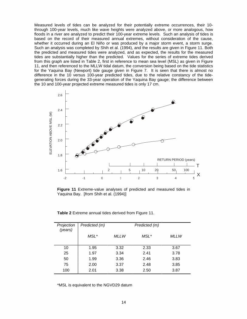
Measured levels of tides can be analyzed for their potentially extreme occurrences, their 10-through 100-year levels, much like wave heights were analyzed above, or more analogous, howfloods in a river are analyzed to predict their 100-year extreme levels. Such an analysis of tides isbased on the record of their measured annual extremes, without consideration of the cause,whether it occurred during an El Niño or was produced by a major storm event, a storm surge.Such an analysis was completed by Shih et al. (1994), and the results are given in Figure 11. Boththe predicted and measured tides were analyzed, and as expected, the results for the measuredtides are substantially higher than the predicted. Values for the series of extreme tides derivedfrom this graph are listed in Table 2, first in reference to mean sea level (MSL) as given in Figure11, and then referenced to the MLLW tidal datum, the conversion being based on the tide statisticsfor the Yaquina Bay (Newport) tide gauge given in Figure 7. It is seen that there is almost nodifference in the 10 versus 100-year predicted tides, due to the relative constancy of the tide-generating forces during the 33-year operation of the Yaquina Bay gauge; the difference betweenthe 10 and 100-year projected extreme measured tides is only 17 cm.
Figure 11 Extreme-value analyses of predicted and measured tides inYaquina Bay. [from Shih et al. (1994)]
Table 2 Extreme annual tides derived from Figure 11.
*MSL is equivalent to the NGVD29 datum
Projection(years)
Predicted (m) Predicted (m)
MSL* MLLW MSL* MLLW
10 1.95 3.32 2.33 3.6725 1.97 3.34 2.41 3.7850 1.99 3.36 2.46 3.8375 2.00 3.37 2.48 3.85
100 2.01 3.38 2.50 3.87
-2 -1 0 1 2 3 4 5X
T1.6
1.8
2.0
2.2
2.4
2.6
2 5 10 20 50 100
RETURN PERIOD (years)
ELE
VAT
ION
AB
OV
E M
SL
(M)

15
The analyses discussed thus far relate to the short-term effects of processes that determine dailyto monthly variations in mean water levels, those that do not permanently alter the mean level ofthe sea. In the longer term, however, a net rise in global (eustatic) sea level has occurred,spanning thousands of years, associated with the melting of glaciers and the return of water to theoceans, and also with a thermal expansion of the ocean's water as it warms. This rise during thepast century is generally placed at 1 to 2 mm/yr, 10 to 20 cm/century, estimated from tide-gaugerecords throughout the world (Komar, 1998b).
The pattern of sea-level rise along the Northwest coast is made complex by on-going changes inthe level of the land. Of importance to coastal erosion is the change in "relative sea level", that is,how the global level of the sea has increased relative to the level of the land. This is what ismeasured by a tide gauge when it's record is averaged for an entire year to determine "mean sealevel" for that year, and then is repeated over many years to see if the level has progressivelychanged. Since the gauge is mounted on the land, it is apparent that the resulting assessment willreflect both the global rise in sea level and the local change in elevation of the land.
Such a determination of the progressive long-term change in relative sea level can be obtainedfrom the 33-year record of measured water levels obtained by the Yaquina Bay tide gauge. Theresult is graphed in Figure 12, a plot of the mean water level each year. It is seen that there hasbeen large fluctuations from year to year, with particularly high water levels associated with the ElNiño events in 1982-83 and 1997-98. However, within those annual variations a long-termprogressive rise in sea level is apparent, one that is on the order of 3.1 mm/yr (31 cm per century).The slightly higher value for the Yaquina Bay tide gauge, compared with the estimate of 1 to 2mm/yr for the global rise in sea level, might suggest that this stretch of the Oregon coast issubsiding. However, the reality is that this 3.1 mm/yr estimate for Newport is uncertain due to thelarge effects of El Niños on the water levels, and the short duration of this record.
Figure 12 Annual values of mean sea level determined from the YaquinaBay tide gauge, demonstrating that temporary high water levels occurredduring the 1982-83 and 1997-98 El Niños, but that there is also aprogressive rise in the sea relative to the land at an average rate of 3.1mm/yr.
This estimate for the relative sea-level rise at Newport is not representative of the entire Northwestcoast in that there are substantial spatial variations in the rates of tectonic change in the level ofthe land along the Oregon and Washington coasts (Komar, 1997). This pattern of changing levelsof the land has been documented by government surveys of geodetic benchmarks used insurveying, monuments that give the precise location and elevation. By resurveying these bench
1964 1968 1972 1976 1980 1984 1988 1992 1996 2000Year
0.05
0.10
0.15
0.20
0.25
0.30
Ele
vatio
n (m
)
Annual Mean Sea Level,South Beach Yaquina Bay, OR
Slope = 0.003 m.yr-1

16
marks every few years, the results document changes in elevations of one benchmark relative toanother. Such an analysis has been undertaken by Vincent (1989) for the benchmarks along thelength of the Oregon coast, and the results are graphed in Figure 13. The data have been furtheranalyzed by linking the benchmark elevation changes with the tide-gauge records at Crescent Cityand Astoria, positioned at the ends of the survey line, so the results in Figure 13 reflect the changein relative sea level. A distinct pattern emerges, with the southern Oregon coast — roughly south ofFlorence — tectonically rising at a faster rate than the global rise in sea level, while most of thenorthern Oregon coast is being slowly submerged by the rising level of the sea.
The rates of sea-level rise relative to the land, Figures 12 and 13, are not large but over the spanof 100 years could amount to 10 to 20 cm change in mean sea level relative to the land. In termsof potential effects on coastal erosion, the rapid tectonic rise of the southern Oregon coast couldresult in a decrease in the total water levels and potential erosion; however, the results in Figure 13indicate that this reduction in water level would amount to only about 10 cm, a small amount that iswithin the uncertainties of assessments of the other water-level processes discussed here. On thenorthern Oregon coast the water is rising relative to the land, and could amount to 20 to 30 cm in100 years, sufficiently large that it should be included in long-range assessments of potentialerosion.
Figure 13 Elevation changes along the Oregon coast, measured bygeodetic surveys (Vincent, 1989). The elevation changes are relative tothe global increase in sea level, with positive values representing a rise inthe land at a higher rate than the increase in sea level, while negativevalues represent the progressive submergence of the land. [from Komar(1997)]
JOINT OCCURRENCES OF EXTREME WAVES ANDWATER LEVELSIn the preceding sections analyses were undertaken to predict extreme storm waves and tides,respectively their 10- through 100-year magnitudes. But it is a combination of high waves andwater levels that results in beach and property erosion. The challenge is to evaluate the jointoccurrences of these processes and their potential erosion impacts. This addition of processes isnot a simple task, and there is no direct established path to evaluate 10- through 100-year jointoccurrences, of the "worst case" erosion event that might impact the Northwest coast.
The uncertainty involves whether or not the respective processes act independently from oneanother, that is, whether they can be expected to occur at the same time or if their joint occurrenceis random chance. For example, the generation of extreme waves by a major storm can beexpected to coincide with a storm surge that elevates the mean water level. On the other hand, ithas been established that the highest monthly-mean water levels are associated with El Niño
42 43 44Latitude
45 46
0
-1
-2
-3
-4
1
2
3
4
Cre
scen
tC
ity
Gol
d B
each
Ban
don
Coo
s B
ay
Flo
renc
e
New
port
Linc
oln
City
Tilla
moo
k
Ast
oria
Land is rising faster thaneustatic sea level rise
Land is being submergedby rising sea level riseLa
nd M
ove
men
t R
elat
ive
to S
ea L
evel
(m
m/y
ear)

17
events, the elevated water being caused in large part by warmer water temperatures and strongerocean currents, factors that are independent of wind-generated waves. It was thought that an ElNiño year would represent a time of reduced waves in the Northwest, due to the southwarddisplacement of the storm tracks so they cross the coast of California rather than the PNW coast(Seymour, 1996). However, during the 1997-98 El Niño a major storm generated deep-watersignificant wave heights of 10 meters along the Northwest coast, previously thought to be the 100-year condition. In spite of that storm occurrence, it remains unlikely that the revised 100-yearstorm with a deep-water significant wave height of 16 meters (Table 1) will strike the coast duringan El Niño, it being more likely that it will occur during a normal or La Niña periods when the stormtracks mainly cross the Northwest. Hence, there is still some validity in separately considering theclimate regimes in analyses of severe ocean conditions that might produce major erosion impacts.That approach will be taken here through analyses of three possible scenarios: (1) An El Niñowinter when the tides are elevated to unprecedented levels, while only moderate storms occur; (2)A normal or La Niña winter when monthly mean water levels and tides are average, but with theoccurrence of a major storm that generates the 100-year wave conditions together with asignificant storm surge; and (3) A "worst case" scenario when something close to a 100-year stormoccurs during an El Niño winter that has elevated mean water levels.
The model that serves as the foundation for assessments of these scenarios is diagrammed inFigure 14. Of interest is the total water level produced by the combined processes, compared withthe elevation of the beach/dune junction; the comparison could also be made with the elevation ofthe toe of a sea cliff, though the subsequent erosional responses of a dune and cliff are clearlydifferent. For the waves to erode the dunes, the elevation of the measured tide (ET) plus the runupof the waves (R) must reach or exceed the elevation of the beach/dune junction (EJ). Here ourinterest focuses on analyses of the extreme occurrences of total water levels, the measured tidesplus the wave runup (ET + R); clearly, the more extreme the total water level, the greater theresulting erosion of dunes and sea cliffs.
Figure 14 Model for the quantitative assessment of foredune erosion,where the elevation of the measured tide (ET) plus the runup of the waves(R) must reach or exceed the elevation of the beach/dune junction (EJ)for erosion to occur.
beach-propertyjunction
wave swash
measured tide levelpredicted tide
NGVD “sea level”
R = wave runup
EJ
ET = measured tide
Property Erosion Modelerosion when + > E R ET J

18
From our earlier discussion it is recognized that the measured tide is governed by the predictedtide, produced by astronomical forces, plus the effects of a number of atmospheric andoceanographic processes. In the present analysis we will take
Measured Tidal Elevation (ET) = Predicted Tide (EPT)+ Monthly Mean Increase (MM)+ Storm Surge (SS)
and these three components of the measured tides will be separately evaluated. We will alsoassume that they act as independent processes, which is true except that our measurements ofmonthly-mean sea levels, Figure 2, are affected somewhat by occurrences of storm surges duringthat particular month. In the evaluations of extreme events undertaken here, some attempt will bemade to account for this tendency toward duplication.
Important to the application of the model is the runup elevation R of the storm waves on the beach.Part of our research has been directed toward obtaining measurements of runup under a range ofdeep-water wave conditions and beach slopes (Ruggiero et al., 1996, in press). Measurements onthe Oregon coast over a wide range of conditions, combined with those obtained by Holman (1986)at the Field Research Facility, Duck, North Carolina, yield the relationship
( ) 21
270 OSO LHS.R = (1)
for the runup elevation (the 2% exceedence elevation), where S is the slope of the beach, HSO isthe deep-water significant wave height, and LO is the deep-water wave length given by
( ) 22 T/gLO π= where T is the wave period, and g is acceleration due to gravity (9.81 m/s). Thecalculations of R in the scenarios developed below therefore depend on values of wave heightsand periods established in our analyses of the Northwest wave climate, specifically on the valuesfor the 10- through 100-year deep-water significant wave heights.
The estimated tide factors and wave runup for the three scenarios are listed in Table 3. The firstentry for each scenario is the predicted tide, EPT, which depends on the astronomical forces of theMoon and Sun, and goes through a monthly cycle between Neap and Spring Tides, the latterachieving the highest levels. From Figure 7, a value of 8.38 ft (2.55 m) MLLW is used, as itrepresents the average of the higher-high predicted tides. That tide level is referenced to the MeanLower-Low Water tidal datum, whereas in assessments of potential coastal erosion it is preferableto have the elevations referenced to a survey datum such as the National Geodetic Vertical Datumof 1929 (NGVD29). According to Figure 7, the difference between the datums is 4.11 ft (1.25 m),so that the 2.55 m MLLW tide level becomes 1.30 m NGVD29. This is the value that is enteredinto Table 3. When the other water-level components are added to this predicted tide, in effectconverting it to an expected measured tide, the resulting water levels will continue to be relative toNGVD29. And finally when the wave runup is added, the resulting total water level will be relativeto NGVD29, which is convenient since land survey elevations are related to that datum, includingthe foredunes and sea cliffs backing the beach.
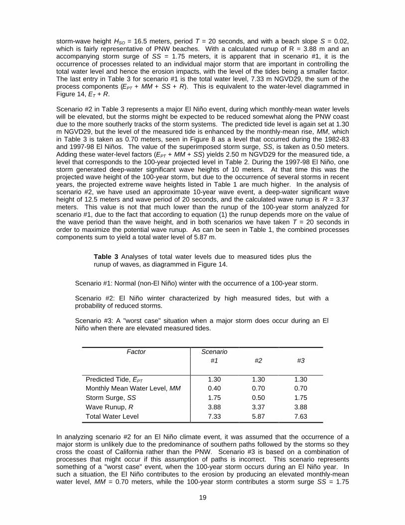
Scenario #1 in Table 3 represents a normal or La Niña year, that is, the opposite to El Niñoconditions. It is seen in Figure 8 that under normal conditions, during the winter the monthly meanwater levels are about 0.40 meter higher than the predicted tides, and this value has been enteredfor MM in Table 3. Most important to scenario #1 is the potential occurrence of a major storm thatwill generate a storm surge and high waves. The best guide we have to such an occurrence is the2-4 March 1999 storm, which produced a storm surge on the order of 1.5 meters on theWashington coast. In terms of wave heights, the 14-meter significant wave heights generated bythat storm now rank as approximately the 50-year event (Table 2), while the projected 100-yearevent has a deep-water wave height of 16 to 17 meters. Presumably, the storm surge would alsobe enhanced during the 100-year storm, being higher than during 2-4 March 1999. Accordingly, inTable 3 the storm surge entry, SS, is set at 1.75 meters, 25 cm higher than during the March 1999event. This estimate assumes an extreme low-pressure storm of approximately 960 mb (about 20mb below the 2-4 March 1999 storm when it crosses the coast), coincident with strong west tosouthwest winds. Finally, the runup R has been calculated with equation (1) using the 100-year
19
storm-wave height HSO = 16.5 meters, period T = 20 seconds, and with a beach slope S = 0.02,which is fairly representative of PNW beaches. With a calculated runup of R = 3.88 m and anaccompanying storm surge of SS = 1.75 meters, it is apparent that in scenario #1, it is theoccurrence of processes related to an individual major storm that are important in controlling thetotal water level and hence the erosion impacts, with the level of the tides being a smaller factor.The last entry in Table 3 for scenario #1 is the total water level, 7.33 m NGVD29, the sum of theprocess components (EPT + MM + SS + R). This is equivalent to the water-level diagrammed inFigure 14, ET + R.
Scenario #2 in Table 3 represents a major El Niño event, during which monthly-mean water levelswill be elevated, but the storms might be expected to be reduced somewhat along the PNW coastdue to the more southerly tracks of the storm systems. The predicted tide level is again set at 1.30m NGVD29, but the level of the measured tide is enhanced by the monthly-mean rise, MM, whichin Table 3 is taken as 0.70 meters, seen in Figure 8 as a level that occurred during the 1982-83and 1997-98 El Niños. The value of the superimposed storm surge, SS, is taken as 0.50 meters.Adding these water-level factors (EPT + MM + SS) yields 2.50 m NGVD29 for the measured tide, alevel that corresponds to the 100-year projected level in Table 2. During the 1997-98 El Niño, onestorm generated deep-water significant wave heights of 10 meters. At that time this was theprojected wave height of the 100-year storm, but due to the occurrence of several storms in recentyears, the projected extreme wave heights listed in Table 1 are much higher. In the analysis ofscenario #2, we have used an approximate 10-year wave event, a deep-water significant waveheight of 12.5 meters and wave period of 20 seconds, and the calculated wave runup is R = 3.37meters. This value is not that much lower than the runup of the 100-year storm analyzed forscenario #1, due to the fact that according to equation (1) the runup depends more on the value ofthe wave period than the wave height, and in both scenarios we have taken T = 20 seconds inorder to maximize the potential wave runup. As can be seen in Table 1, the combined processescomponents sum to yield a total water level of 5.87 m.
Table 3 Analyses of total water levels due to measured tides plus therunup of waves, as diagrammed in Figure 14.
Scenario #1: Normal (non-El Niño) winter with the occurrence of a 100-year storm.
Scenario #2: El Niño winter characterized by high measured tides, but with aprobability of reduced storms.
Scenario #3: A "worst case" situation when a major storm does occur during an ElNiño when there are elevated measured tides.
In analyzing scenario #2 for an El Niño climate event, it was assumed that the occurrence of amajor storm is unlikely due to the predominance of southern paths followed by the storms so theycross the coast of California rather than the PNW. Scenario #3 is based on a combination ofprocesses that might occur if this assumption of paths is incorrect. This scenario representssomething of a "worst case" event, when the 100-year storm occurs during an El Niño year. Insuch a situation, the El Niño contributes to the erosion by producing an elevated monthly-meanwater level, MM = 0.70 meters, while the 100-year storm contributes a storm surge SS = 1.75
Factor Scenario#1 #2 #3
Predicted Tide, EPT 1.30 1.30 1.30Monthly Mean Water Level, MM 0.40 0.70 0.70Storm Surge, SS 1.75 0.50 1.75Wave Runup, R 3.88 3.37 3.88Total Water Level 7.33 5.87 7.63

20
meters to the measured tide, while the generated waves add a runup R = 3.88 meters, giving acalculated total water level of 7.63 meters (Table 3).
DISCUSSION OF RESULTS AND POTENTIAL EROSIONThe analyses of the three scenarios presented in Table 3 differ considerably from the results, hadsimilar analyses been undertaken in 1996. At that time the 100-year projected extreme deep-waterwave height was about 10 meters. There was a high level of uncertainty in that projection due tothe shortness of records of wave measurements. But the largest change in the 10- through 100-year wave projections has resulted from the unprecedented number of major storms during thewinters of 1997-98 and 1998-99, with a total of five storms having exceeded the earlier projectionof 10 meters for the 100-year event. Analyses presented here, Table 1, indicate that the 100-yearstorm should generate deep-water significant wave heights on the order of 16 to 17 meters, withthe further projection that we can routinely expect 10-meter waves, approximately every 5 years. Itis uncertain what change in climate has brought about this recent increase in storm-wave heights.It is clear that for the past 25 years there has been a progressive increase in wave heights andperiods along the PNW coast (Allan and Komar, 2000, in press). The climate factors responsiblefor this progressive increase have not been determined, and without such an identification it is notpossible to predict whether this trend will continue in the future. If it does, the extreme waves inthe future will be even greater that the projected values given in Table 1, the result of an analysisprocedure that assumes the wave climate is static, with no long-term trend.
The other major change in Table 3, compared with similar estimates made in the past, involves thelevel of enhancement of the tide by the occurrence of a storm surge. As of 1996, analyses ofstorm surges had indicated they would typically raise the water level by 15 to 30 cm, and during asevere storm might raise it by 50 cm. This view changed when the storm of 2-4 March 1999 raisedthe measured tide above the predicted tide by about 1.75 meters as measured by the Toke Pointtide gauge in Willapa Bay. In the analyses presented in this report, it is suggested that about 1.5meters of this actually represented the storm surge, the balance in the water-level increase havingbeen produced by the monthly-mean water level. This occurrence is 1-meter higher than the 50-cm elevation previously projected for an extreme storm surge.
In that both the increased wave heights and storm surge elevations are associated with theoccurrence of major storm events, the revisions in Table 3 compared with estimates in 1996 clearlyreflect the increased storm intensities that have occurred in recent years. Scenarios #1 and #2clearly reflect that experience. Scenario #1 is basically for the occurrence of what is now projectedto be the 100-year storm event. In calculating the component factors, we have adopted somethingof a "worst case" situation wherein the storm and its generated waves and surge strike the coast ata time of high tides. However, in all scenarios we used an average for the predicted higher-hightides, rather than using the greater elevation of a Spring Tide. So in that sense the scenarios donot represent worst-case events. The monthly-mean water levels (MM) entered into scenarios #1and #2 have been well documented by measurements, Figure 2, and do not represent particularlyextreme values based on past experience. The wave runup (R) is a reasonable estimate exceptthat its calculation is based on a wave period T = 20 seconds. An examination of the largeststorms, those that were used to project the extreme wave heights, demonstrated that a number ofthem had periods up to 20 seconds, whereas others had periods as low as 12 seconds. In that thecalculation of R, equation (1), is very sensitive to the wave period, being directly proportional to T,whether the storm has a period of 20 or 12 seconds will result in a substantial difference in thelevel of the wave runup. In that we used a value of 20 seconds in developing the scenarios inTable 3, we again have based the assessment on a worst-case condition.
The results for the total water levels in Table 3 suggest that in terms of the resulting coastalerosion, an El Niño climate event should have less impact on the coast than a "normal" or La Niñawinter. This finding appears to conflict with our experience that significant erosion occurs along thecoasts of Oregon and Washington during an El Niño (Komar, 1986, 1997, 1998a; Kaminsky et al.,1998). However, most of the El Niño related erosion is not necessarily the result of extremestorms and water levels, the factors analyzed in Table 3, but is due instead to the shift in the wavedirections to a more southwesterly quadrant, producing a northward movement of beach sandwithin the littoral cells between headlands. During both the 1982-83 and 1997-98 El Niños, it was
21
observed that the most severe beach and property erosion occurred in "hot spot" zones north ofheadlands and north of migrating tidal inlets, produced by the northward movement of beach sand.Those occurrences of erosion demonstrate the fact that there are other factors and processesimportant to the problem that it is not simply due to extreme levels of tides and wave runup asanalyzed in Table 3. However, during a normal or La Niña winter, when the storms come moredirectly across the Northwest coast, the northward movement of sand as occurs during an El Niñois not an important factors in the erosion, so the total water level of scenario #1, governed mainlyby the occurrence of a major storm, is likely to dominate the resulting erosion, which will also tendto develop along the full length of the littoral cell, rather than being localized in "hot spot" areas asduring an El Niño. This coast-wide pattern of erosion was illustrated by that which occurred alongthe Northwest during the 2-4 March 1999 storm, even though the calculated maximum total waterlevels reached to only 4 to 5 meters NGVD29, because the storm struck the coast at a time ofrelatively modest predicted tides (Komar et al., 1999).
Normally one attempts to quantitatively estimate the probability of the occurrence of a naturalevent; in the present application, the probabilities of the calculated total water levels for the threescenarios in Table 3. It should be recognized that although we tend to express the probability, forexample, as the "100-year event", that event actually represents the 1-in-100 probability ofoccurrence during any one year (in other words, a 1% chance of occurrence in any given year). Itis difficult evaluate this probability when one is considering the joint occurrences of multipleprocesses, each of which has its own probability of occurrence. To make such an analysis, wemight separate the processes that control the mean water levels — measured tides — from therunup of the storm waves. If these two components were completely independent in theiroccurrences, then one might couple the 2-year water level with the 50-year wave runup occurrenceto arrive at a 100-year combined event (alternately, we could use 10-year combinations). But as wehave seen, an important part of the measured tide is the storm surge, which occurs at the time ofthe enhanced wave generation and runup, so a division between measured tides and wavegeneration cannot be considered as independent processes. A more rational division is betweenthe predicted tides plus the monthly-mean water levels as affected by water temperatures andoffshore currents, versus the storm-occurrence processes of wave generation (runup) and thestorm surge. To a degree such a division was made in scenarios #1 and #2, where #1 representsthe 100-year storm while the combination of predicted tide and monthly mean water level is a 1-year assessment. In the opposite direction, scenario #2 represents an El Niño winter when thewater levels are close to a 100-year occurrence, while the storm wave heights are more moderateand of frequent occurrence.
The selections of conditions for scenarios #1 and #2 were based on the desire to have thecombined results sum to a total water level that has an approximate 1-in-100 probability ofoccurrence. However, in that those specific climate regimes do not occur every year, theprobabilities are lower. In that most years are "normal", those years combined with theoccurrences of La Niñas to give scenario #1 have close to a 1-in-1 probability, so the total waterlevel calculated in Table 3 for scenario #1 can be taken as having close to a 1-in-100 probability.In that strong El Niños are infrequent, the projected water level in Table 3 for scenario #2 has a lowprobability, much less than 1-in-100, but this is perhaps irrelevant since most of the erosion duringan El Niño has the "hot spot" pattern associated with the northward movement of beach sand withinthe littoral cells, rather than being caused by total water levels.
The greatest potential impact to the Northwest coast would come from scenario #3 in Table 3,which in effect combines the major impacts of an El Niño (including the northward movement ofbeach sand), and the occurrence of a 100-year storm as analyzed for scenario #1. Although stormsystems do tend to be displaced toward the south during an El Niño, so we might expect somereduction in wave-energy levels as hypothesized by Seymour (1996), the possibility cannot beruled out entirely that sometime in the future we will experience a 100-year storm event during anEl Niño year. Considering the degree to which our ideas and assessments of the processes havechanged during the past few years due to the occurrence of much stronger storms, we shouldhesitate to rule out the possibility of scenario #3.

22
In terms of total water levels, Table 3, the difference between scenarios #1 and #3 only amount to30 cm. However, management planning for scenarios #1 and #3 is different in that #3 includes thehot-spot erosion impacts as well as the most extreme wave runup and total water levels. Thus,there would be the coast-wide erosion inherent in the major storm scenario #1, with a localized hot-spot erosion produced by the northward transport of sediment within the littoral cells, characteristicof an El Niño. To a degree, the erosion experienced during the winter of 1998-99 demonstrates thepotential impacts in that the Northwest beaches had not fully recovered from the 1997-98 El Niño,when they were further eroded by the series of major storms of the 1998-99 La Niña. However, thepotential impacts of scenario #3 would be still greater than that recent experience, due to thesignificantly higher total water level of scenario #3 than occurred during the winters of 1997-98 and1998-99.

23
REFERENCESAllan, J.C., and P.D. Komar (2000) Spatial and Temporal Variations in the Wave Climate of theNorth Pacific: Report to the Oregon Department of Land Conservation and Development, 46 pp.
Allan, J.C., and P.D. Komar (in press) Are ocean wave heights increasing in the Eastern NorthPacific?: EOS..
Hamilton, S.F. (1973) Oregon Estuaries: Oregon Division of State Lands, Salem.
Helmsley, J.M., and R.M. Brooks (1989) Waves for coastal design in the United States: Journal ofCoastal Reserch, v. 5, p. 639-663.
Holman, R.A. (1986) Extreme value statistics for wave run-up on a natural beach: CoastalEngineering, v. 9, p. 527-544.
Kaminsky, G.M., P. Ruggioer and G. Gelfenbaum (1998) Monitoring coatal change in southwestWashington and northwest Oregon during the 1997/98 El Niño: Shore & Beach, v. 66, n. 3, p. 42-51.
Komar, P.D. (1986) The 1982-83 El Niño and erosion on the coast of Oregon, Shore & Beach, v.54, p. 3-12.
Komar, P.D. (1997) The Pacific Northwest Coast: Living with the Shores of Oregon andWashington: Duke University Press.
Komar, P.D. (1998a) The 1997-98 El Niño and erosion of the Oregon coast: Shore & Beach, v. 66,n. 3, p. 33-41.
Komar, P.D. (1998b) Beach Processes and Sedimentation: Prentice-Hall Inc., Upper Saddle River,NJ.
Komar, P.D., G. Diaz-Mendez, and J.J. Marra (1999) El Niño and La Niña – Erosiion Impactsalong the Oregon Coast: Report to the Oregon Department of Land Conservation andDevelopment, 40 pp.
Longuet-Higgins, M.S. (1950) A theory of the origin of microseisms: Philosophical Transactions ofthe Royal Society of London, v. A243, p. 1-35.
Ruggiero, P., P.D. Komar, W.G. McDougal, and R.A. Beach (1996) Extreme water levels, waverunup and coastal erosion: Proceedings 25th International Conference on Coastal Engineering,Amer. Soc. Civil Engrs., pp. 2793-2805.
Ruggiero, P., P.D. Komar, W.G. McDougal, J.J. Marra and R.A. Beach (in press) Wave runup,extreme water levels and the erosion of properties backing beaches: Journal of Coastal Research.
Seymour, R.J. (1996) Wave climate variability in Southern California: Journal of Waterway, Port,Coastal and Ocean Engineering, Amer. Soc. Civil Engrs., v. 122, n. 4, p. 182-186.
Seymour, R.J. (1998) Effects of El Niño on the West Coast wave climate: Shore & Beach, v. 66, n.3, p. 3-6.
Seymour, R.J., R.R. Strange, D.R. Cayan and R.A. Nathan (1984) Influence of El Niños onCalifornia's wave climate: Proceedings 19th Coastal Engineering Conference, Amer. Soc. CivilEngr., pp. 577-592.

24
Seymour, R.J., M.H. Sessions, and D. Castel (1985) Automated remote recording and analysis ofcoastal data: Journal of Waterway, Port, Coastal and Ocean Engineering, 111: 388-400.
Shih, S.-M., P.D. Komar, K.J. Tillotson, W.G. McDougal and P. Ruggiero (1994) Wave runup andsea-cliff erosion: Proceedings 24th International Coastal Engineering Conference, Amer. Soc. CivilEngrs., pp. 2170-2184.
Tillotson, K.J., and P.D. Komar (1997) The wave climate of the Pacific Northwest (Oregon andWashington): A comparison of data sources: Journal of Coastal Research, v. 13, p. 440-452.
Vincent, P. (1989) Geodetic Deformation of the Oregon Cascadia Margin: Master's thesis,University of Oregon.
Zopf, D.O., H.C. Creech, and W.H. Quinn (1976) The wavemeter: A land-based system formeasuring nearshore ocean waves: MTS Journal, v. 10, p. 19-25.