face recognition jammer using image morphing recognition jammer using image morphing jonathan wu...

Face Recognition Jammer using Image Morphing

Jonathan Wu

Boston University Department of Electrical and Computer Engineering

8 Saint Mary’s Street Boston, MA 02215 www.bu.edu/ece

Dec 18, 2011

Technical Report No. ECE-2011-03

Contents

1. Introduction ...............................................................................................1

2. Literature Review .....................................................................................1

3. Problem Statement....................................................................................2

3.1 Active Shape Models ...........................................................................4

3.2 Extract Facial Region from Image ..................................................5

3.3 Facial Structure: Triangular mesh ....................................................6

3.4 Interpolating between facial landmarks ...........................................6

3.5 Warp faces ...........................................................................................7

3.6 Average between faces ........................................................................8

3.7 Morphing between multiple faces......................................................10

3.8 Evaluation Overview ..........................................................................11

3.9 Dataset ..................................................................................................12

3.10 Building training set .........................................................................12

3.11 Deciding target face(s) ......................................................................15

3.12 Evaluation ..........................................................................................16

4. Implementation .........................................................................................17

5. Experimental results .................................................................................17

6. Conclusions ................................................................................................17

6.1 Future Work ........................................................................................18

7. References ..................................................................................................18

List of Figures

Figure 1.1: Averaging of two faces 1

Figure 2.1: Misra, CVDazzle 2

Figure 3.1: Blending a base face with a target face using facial morphing 2

Figure 3.2: Overview of facial morphing 3

Figure 3.1.1: Active Shape model landmarks 4

Figure 3.2.1: Extracting facial regions from an image 5

Figure 3.3.1: Circumcircle and facial mesh 6

Figure 3.4.1: Diagram of base and target meshes 6

Figure 3.5.1: 6-parameter affine transform 7

Figure 3.5.2: Homogenous affine transform 7

Figure 3.6.1: Graphic overview of morphing process 8

Figure 3.6.2: Morphing results of facial images 9

Figure 3.8.1: Evaluation of query facial image overview 11

Figure 3.9.1: Sample of the FEI Dataset 12

Figure 3.10.1: Mean face and eigenfaces 14

Figure 5.1: SSD graphical results 17

1 Face Recognition Jammer – Jonathan Wu

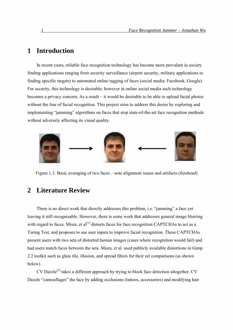
1 Introduction

In recent years, reliable face recognition technology has become more prevalent in society

finding applications ranging from security surveillance (airport security, military applications to

finding specific targets) to automated online tagging of faces (social media: Facebook, Google).

For security, this technology is desirable; however in online social media such technology

becomes a privacy concern. As a result – it would be desirable to be able to upload facial photos

without the fear of facial recognition. This project aims to address this desire by exploring and

implementing “jamming” algorithms on faces that stop state-of-the-art face recognition methods

without adversely affecting its visual quality.

Figure 1.1: Basic averaging of two faces – note alignment issues and artifacts (forehead)

2 Literature Review

There is no direct work that directly addresses this problem, i.e. “jamming” a face yet

leaving it still recognizable. However, there is some work that addresses general image blurring

with regard to faces. Misra, et al[1] distorts faces for face recognition CAPTCHAs to act as a

Turing Test, and proposes to use user inputs to improve facial recognition. These CAPTCHAs

present users with two sets of distorted human images (cases where recognition would fail) and

had users match faces between the sets. Misra, et al. used publicly available distortions in Gimp

2.2 toolkit such as glass tile, illusion, and spread filters for their set comparisons (as shown

below).

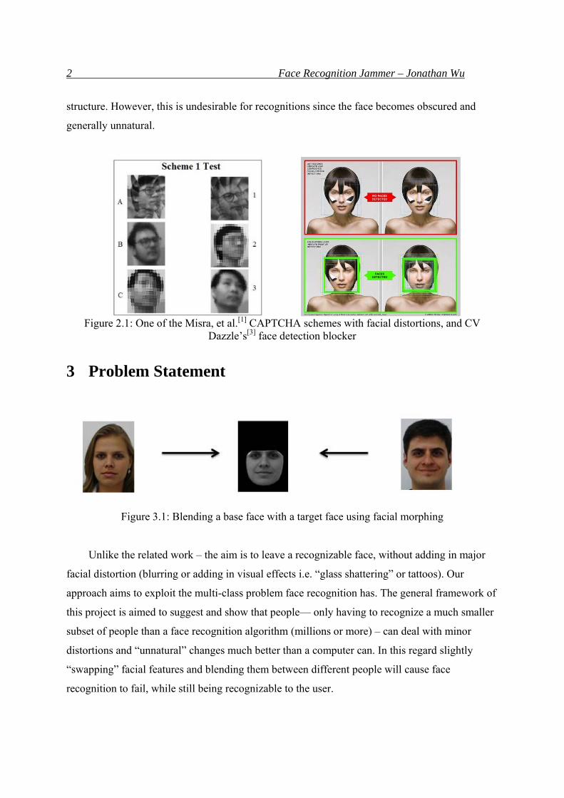
CV Dazzle[3] takes a different approach by trying to block face detection altogether. CV

Dazzle “camouflages” the face by adding occlusions (tattoos, accessories) and modifying hair


structure. However, this is undesirable for recognitions since the face becomes obscured and

generally unnatural.

Figure 2.1: One of the Misra, et al.[1] CAPTCHA schemes with facial distortions, and CV

Dazzle’s[3] face detection blocker

3 Problem Statement

Figure 3.1: Blending a base face with a target face using facial morphing

Unlike the related work – the aim is to leave a recognizable face, without adding in major

facial distortion (blurring or adding in visual effects i.e. “glass shattering” or tattoos). Our

approach aims to exploit the multi-class problem face recognition has. The general framework of

this project is aimed to suggest and show that people— only having to recognize a much smaller

subset of people than a face recognition algorithm (millions or more) – can deal with minor

distortions and “unnatural” changes much better than a computer can. In this regard slightly

“swapping” facial features and blending them between different people will cause face

recognition to fail, while still being recognizable to the user.


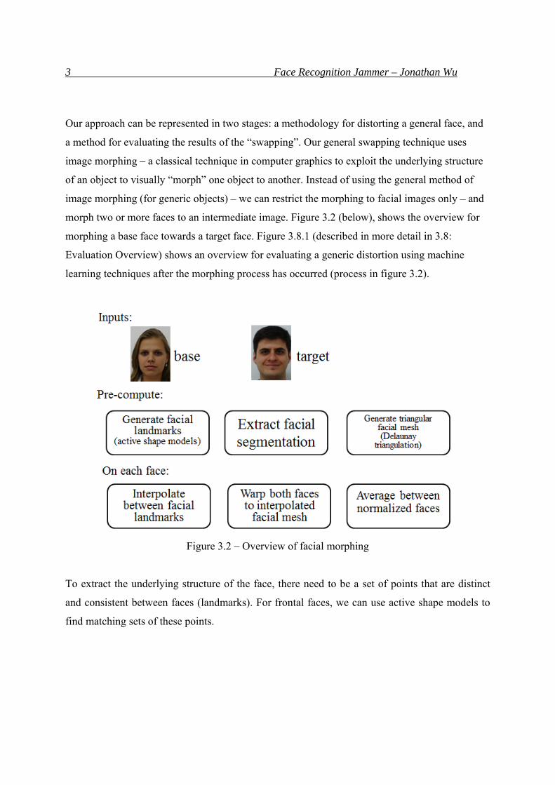
Our approach can be represented in two stages: a methodology for distorting a general face, and

a method for evaluating the results of the “swapping”. Our general swapping technique uses

image morphing – a classical technique in computer graphics to exploit the underlying structure

of an object to visually “morph” one object to another. Instead of using the general method of

image morphing (for generic objects) – we can restrict the morphing to facial images only – and

morph two or more faces to an intermediate image. Figure 3.2 (below), shows the overview for

morphing a base face towards a target face. Figure 3.8.1 (described in more detail in 3.8:

Evaluation Overview) shows an overview for evaluating a generic distortion using machine

learning techniques after the morphing process has occurred (process in figure 3.2).

Figure 3.2 – Overview of facial morphing

To extract the underlying structure of the face, there need to be a set of points that are distinct

and consistent between faces (landmarks). For frontal faces, we can use active shape models to

find matching sets of these points.


3.1 Active Shape Models (ASM)

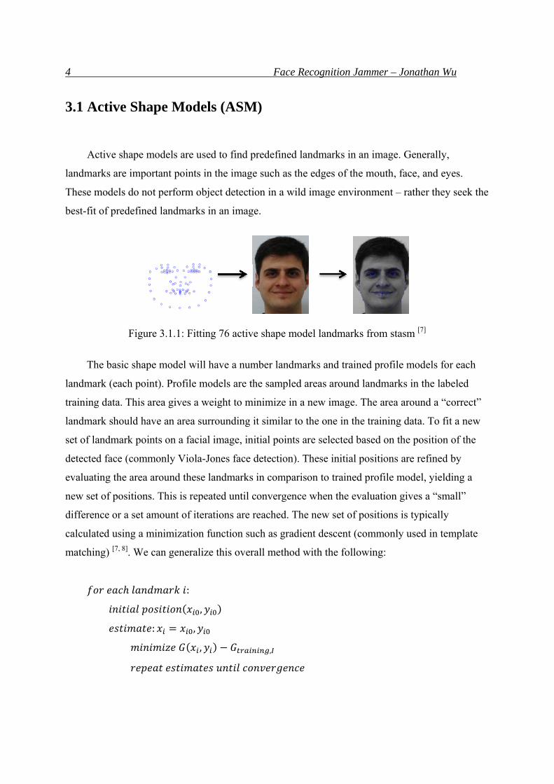
Active shape models are used to find predefined landmarks in an image. Generally,

landmarks are important points in the image such as the edges of the mouth, face, and eyes.

These models do not perform object detection in a wild image environment – rather they seek the

best-fit of predefined landmarks in an image.

Figure 3.1.1: Fitting 76 active shape model landmarks from stasm [7]

The basic shape model will have a number landmarks and trained profile models for each

landmark (each point). Profile models are the sampled areas around landmarks in the labeled

training data. This area gives a weight to minimize in a new image. The area around a “correct”

landmark should have an area surrounding it similar to the one in the training data. To fit a new

set of landmark points on a facial image, initial points are selected based on the position of the

detected face (commonly Viola-Jones face detection). These initial positions are refined by

evaluating the area around these landmarks in comparison to trained profile model, yielding a

new set of positions. This is repeated until convergence when the evaluation gives a “small”

difference or a set amount of iterations are reached. The new set of positions is typically

calculated using a minimization function such as gradient descent (commonly used in template

matching) [7, 8]. We can generalize this overall method with the following:

:

,

: ,

, ,


, ,

In this project, feature points were generated from the stasm [7] library which uses a more

sophisticated ASM that takes additional constraints into account (such as taking spatial

properties).

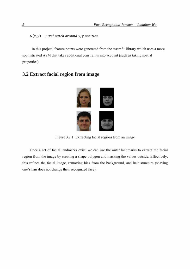
3.2 Extract facial region from image

Figure 3.2.1: Extracting facial regions from an image

Once a set of facial landmarks exist, we can use the outer landmarks to extract the facial

region from the image by creating a shape polygon and masking the values outside. Effectively,

this refines the facial image, removing bias from the background, and hair structure (shaving

one’s hair does not change their recognized face).


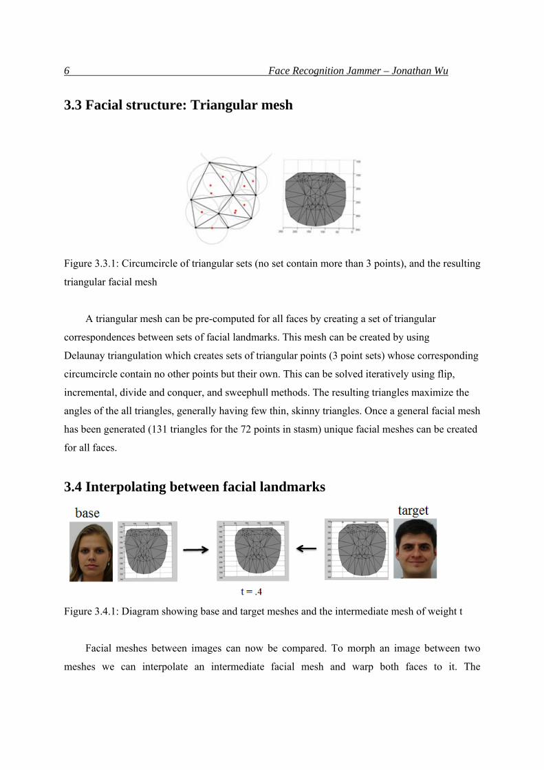
3.3 Facial structure: Triangular mesh

Figure 3.3.1: Circumcircle of triangular sets (no set contain more than 3 points), and the resulting

triangular facial mesh

A triangular mesh can be pre-computed for all faces by creating a set of triangular

correspondences between sets of facial landmarks. This mesh can be created by using

Delaunay triangulation which creates sets of triangular points (3 point sets) whose corresponding

circumcircle contain no other points but their own. This can be solved iteratively using flip,

incremental, divide and conquer, and sweephull methods. The resulting triangles maximize the

angles of the all triangles, generally having few thin, skinny triangles. Once a general facial mesh

has been generated (131 triangles for the 72 points in stasm) unique facial meshes can be created

for all faces.

3.4 Interpolating between facial landmarks

Figure 3.4.1: Diagram showing base and target meshes and the intermediate mesh of weight t

Facial meshes between images can now be compared. To morph an image between two

meshes we can interpolate an intermediate facial mesh and warp both faces to it. The


intermediate facial mesh can be generated by weighing between both sets of facial landmarks as

follows:

:

, 1 ∗ . ∗ ,

Wecanusethefollowingnotation:

:

, :

, :

, :

: 0 1 , ,

1

3.5 Warp faces

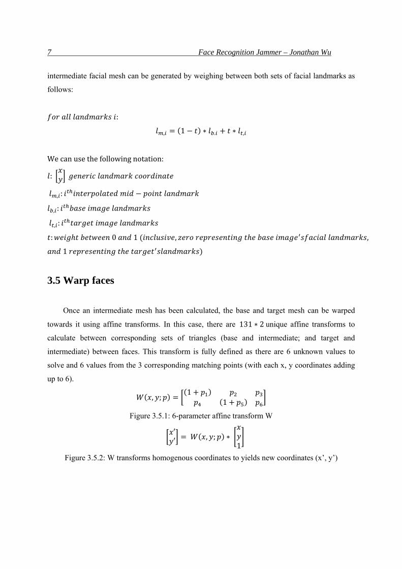
Once an intermediate mesh has been calculated, the base and target mesh can be warped

towards it using affine transforms. In this case, there are 131 ∗ 2unique affine transforms to

calculate between corresponding sets of triangles (base and intermediate; and target and

intermediate) between faces. This transform is fully defined as there are 6 unknown values to

solve and 6 values from the 3 corresponding matching points (with each x, y coordinates adding

up to 6).

, ;1

1

Figure 3.5.1: 6-parameter affine transform W

′′ , ; ∗

1

Figure 3.5.2: W transforms homogenous coordinates to yields new coordinates (x’, y’)


:

1. 131 3 , ′, ′ , :

, ′ , ′ , ′

, ′ , ′ , ′ , ; ∗

, , ,

, , ,

1 1 1

. 3 ,. ,

.

2. , :

, ,

, ,

, .

3.6 Average between faces

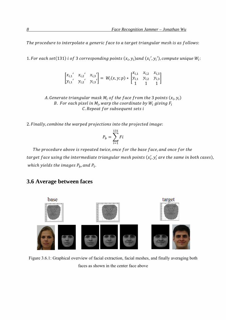
Figure 3.6.1: Graphical overview of facial extraction, facial meshes, and finally averaging both

faces as shown in the center face above


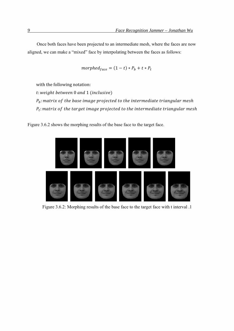
Once both faces have been projected to an intermediate mesh, where the faces are now

aligned, we can make a “mixed” face by interpolating between the faces as follows:

1 ∗ ∗

withthefollowingnotation:

: 0 1

:

:

Figure 3.6.2 shows the morphing results of the base face to the target face.

Figure 3.6.2: Morphing results of the base face to the target face with t interval .1


3.7 Morphing between multiple faces

It is generally possible to morph (project to intermediate mesh, and blend) with multiple

N-target faces. For example, one novel method could perform the following:

1.) Generate intermediate mesh weighing between multiple faces

:

, 1 ∗ . ∗ , ,

:

:

, :

, :

, , :

: 0 1 , ,

1

2.) Warp all faces to intermediate mesh using affine warping in 3.5: Warping faces, which

generates P , values

3.) Blend between faces

1 ∗ ∗ ,

usingthenotation:

: 0 1

:

, :


However, for the purposes of evaluation and available processing time, the base face was

morphed with one target face.

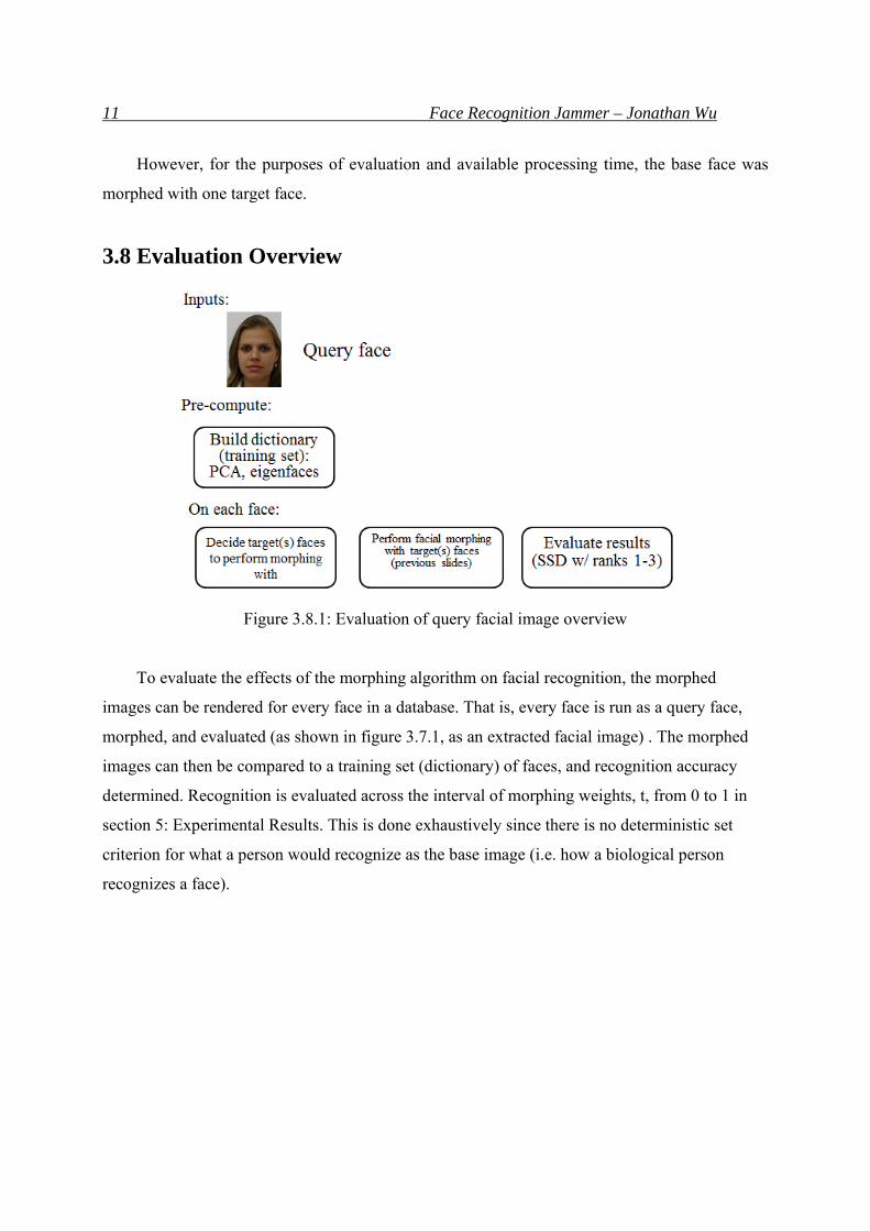
3.8 Evaluation Overview

Figure 3.8.1: Evaluation of query facial image overview

To evaluate the effects of the morphing algorithm on facial recognition, the morphed

images can be rendered for every face in a database. That is, every face is run as a query face,

morphed, and evaluated (as shown in figure 3.7.1, as an extracted facial image) . The morphed

images can then be compared to a training set (dictionary) of faces, and recognition accuracy

determined. Recognition is evaluated across the interval of morphing weights, t, from 0 to 1 in

section 5: Experimental Results. This is done exhaustively since there is no deterministic set

criterion for what a person would recognize as the base image (i.e. how a biological person

recognizes a face).


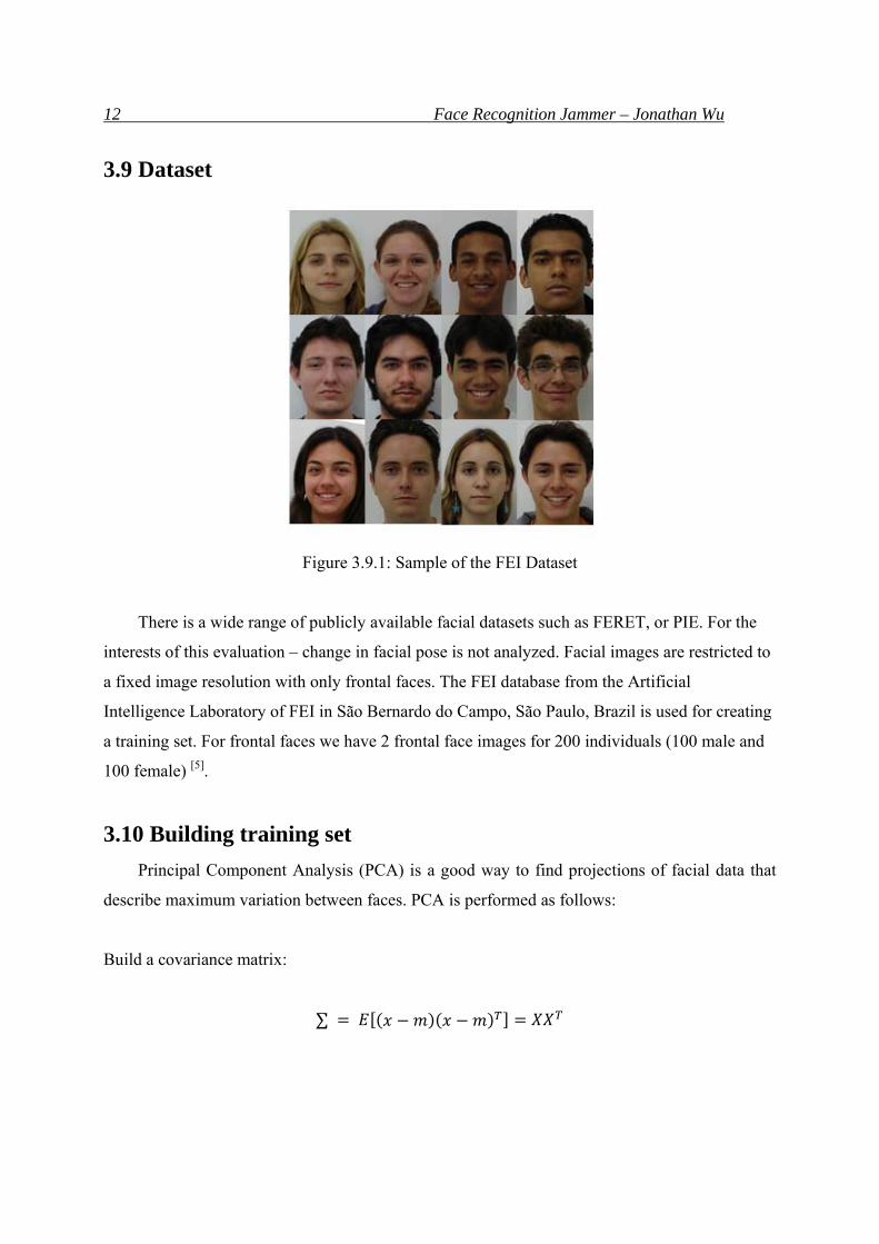
3.9 Dataset

Figure 3.9.1: Sample of the FEI Dataset

There is a wide range of publicly available facial datasets such as FERET, or PIE. For the

interests of this evaluation – change in facial pose is not analyzed. Facial images are restricted to

a fixed image resolution with only frontal faces. The FEI database from the Artificial

Intelligence Laboratory of FEI in São Bernardo do Campo, São Paulo, Brazil is used for creating

a training set. For frontal faces we have 2 frontal face images for 200 individuals (100 male and

100 female) [5].

3.10 Building training set

Principal Component Analysis (PCA) is a good way to find projections of facial data that

describe maximum variation between faces. PCA is performed as follows:

Build a covariance matrix:

∑


withthefollowingnotation:

∑:

:

:

: , ∗

Extracteigenvalues λscalar , andeigenvectors alsocalledeigenfaces, v of∑:

∑

However, solving for eigenvectors and eigenvalues has high dimensionality in this case

(covariance matrix is D by D dimensionality with D >> N)

To reduce computation we can use the kernel trick which allows us to evaluate a covariance

matrix with N by N dimensionality.

The first step is to premultiply both sides of the equation by XT:

∑

λv

We can replace the XTv term with v :

Afterwards, we compute the eigenvalues for (the same λasbefore ) and the

v eigenvectors. These vectors premultiplied by the X matrix will then produce the eigenfaces, v,

(vectors of the original length D) from v , N-1 length eigenvectors (from

earlier).


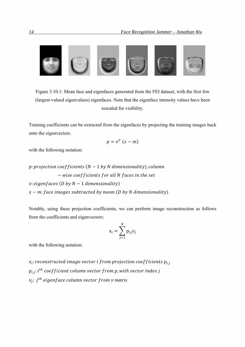
Figure 3.10.1: Mean face and eigenfaces generated from the FEI dataset, with the first few

(largest-valued eigenvalues) eigenfaces. Note that the eigenface intensity values have been

rescaled for visibility.

Training coefficients can be extracted from the eigenfaces by projecting the training images back

onto the eigenvectors.

with the following notation:

: 1 ,

: 1

:

Notably, using these projection coefficients, we can perform image reconstruction as follows

from the coefficients and eigenvectors:

x p ,

with the following notation:

: ,

, : ,

: matrix


Performing PCA on a dataset creates a set of projection coefficients which are maximally

varied which is useful later for more accurate classification.

3.11 Deciding target face(s)

For each query face, a target face is desired to be morphed with.

For our purposes, two types of faces were made as targets:

- The face with the furthest coefficient SSD (sum squared distance), person themselves

excluded

- The face with the closest coefficient SSD, person themselves excluded

Since we know the training coefficients of the query face, we simply need to compute its SSD

with regards to the other training faces and sort them.

SSD is denoted as follows:

We denote the set of , , … ,

Two methods of finding the target face, :

min ,

And:

max ,

usingnotation:

:

:

:

:

: ,

:

: 1


3.12 Evalutation

After determining a target face(s) and generating a morphed facial image, we can perform

classification based on nearest projection coefficient SSD. We can do this as follows (using

notation in 3.11)

First compute the coefficicients for the morphed face:

Calculate SSD values across all training set faces:

, , , … ,

Classify the morphing as correct if:

min ,

We can extend this classification to multiple k-ranks (if any k-closest is correct):

min , , , , … , ,

⋃ …⋃ }

, :

In comparison to other classification techniques such as state vector machines (SVMs), this

algorithm does not draw decision boundaries in space. Rather, it finds the closest known values

spatially and labels it as those. However, it may be useful to note that SVMs may not have

perfect training accuracy (depending on the decision boundaries), while SSD will always have

perfect training accuracy, as the smallest SSD of a trained face will always be 0 (being itself).

This is generally the case, since SVMs optimize for testing data (modeling for unseen faces

based on known faces), while SSDs is optimized for known data. In this regard, since morphed

images are composed from training data, SSD was thought to be suitable for preliminary

analysis.


4 Implementation

Implementation was mostly done in MATLAB (morphing and evaluation), only using the

stasm library to pre-compute facial landmarks. Computation was done on a personal laptop with

a i7-2630QM CPU @ 2.00 GHz, and 6GB of DRAM.

5 Experimental results

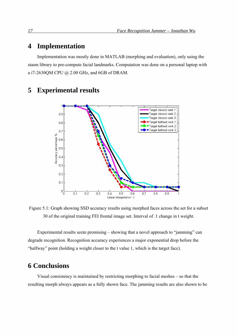
Figure 5.1: Graph showing SSD accuracy results using morphed faces across the set for a subset

30 of the original training FEI frontal image set. Interval of .1 change in t weight.

Experimental results seem promising – showing that a novel approach to “jamming” can

degrade recognition. Recognition accuracy experiences a major exponential drop before the

“halfway” point (holding a weight closer to the t value 1, which is the target face).

6 Conclusions

Visual consistency is maintained by restricting morphing to facial meshes – so that the

resulting morph always appears as a fully shown face. The jamming results are also shown to be


significant – increase in classification rank does not cause a huge increase in accuracy, eluding

that the morphed face is usually not within the nearest SSD neighbors

6.1 Future Work

There is a wide range of future work that can be done. The affine transforms have graphical

artifacts that can be rectified using graphical in-painting. Also, the recognition algorithm can be

scaled to larger sets (modern datasets have far more training images which are more robust

against occlusions by using realistic images from Flickr or Picasa). Furthermore, classification

can be run more exhaustively for finer values of weight t. Also, these blending, morphing and

recognition methods can also take into account facial regions (i.e. eyes, nose, ear, and mouth).

One example is in the recognition algorithm which can be expanded to a hierarchical model

using machine learning with voting by parts (each facial part has its own classifier).

7 References

[1] Misra D., Gaj, K; Face Recognition CAPTCHAs. AICT-ICIW, 2006. [2] Turk, M., Pentland, A; Face Recognition Using Eigenfaces. CVPR, 1991. [3] http://cvdazzle.com/ [5] http://fei.edu.br/~cet/facedatabase.html [6] S. Milborrow and F. Nicolls. Locating Facial Features with an Extended Active Shape Model. ECCV 2008. http://www.milbo.users.sonic.net/stasm/ [7] T. F. Cootes and C. J. Taylor. Technical Report: Statistical Models of Appearance for Computer Vision. The University of Manchester School of Medicine, 2004. www.isbe. man.ac.uk/~bim/Models/app_models.pdf.

face recognition jammer using image morphing recognition jammer using image morphing jonathan wu...

Documents