FARM LAND VALUE AND RURAL ROADS SERVICE IN ELLIS COUNTY, TEXAS

1955-58

by

William G. Adkins James E. Frierson

Russell H. Thompson

A Special Report to the Bureau of Public Roads,

United States Department of Commerce

BULLETIN NO. 1~

E 89-60

June, 1960

Texas Transportation Institute

A. & M. College of Texas

College Station, Texas

ACKNOWLEDGEMENT

The authors are especially grateful for the cooperation of the land buyers in Ellis County who relinquished valuable time from busy schedules to answer questions about the land they had purchased. Their help was quite necessary to the study and they responded in a most acceptable manner.

Appreciation also is expressed to the several county and other government officials who aided in the study. The County Clerk's Office and the Agricultural Stabilization and Conservation Office helped the researchers to determine the land which sold and to locate the persons who bought it. The ASC office also furnished productivity information.

Finally, the contribution of Mr. Billy Baker and Mr. B. J. Rosser is recognized. These young men, who worked long hours conducting interviews and inspecting pub­lic records, performed their work dutifully and well.

Finally, acknowledgment is due of the Data Processing Center, A. & M. Col­lege of Texas, and the Bureau of Public Roads, United States Department of Com­merce, for their continued cooperation throughout the study.

TABLE OF CONTENTS

Page SUMMARY AND CONCLUSIONS _____________________________________________________________________ 5

CHARACTERISTICS OF ELLIS COUNTY-------------------------------------------------------------- 9 Population and Employment _______________________________________________________________________ 9

Farm Characteristics----------------------------------------------------------------------------- 9 Road Facilities __________________________________________________________________________________ 10

SCOPE OF THE STUDY AND NOTES ON METHOD ____________________________________________________ ll

Number of Sales _________________________________________________________________________________ 11

Summary of Sales Data ___________________________________________________________________________ ll

Variations of Farm Characteristics and Land Prices __________________________________________________ ll

Method of Analysis _______________________________________________________________________________ 13

Variables Considered in Regression Analyses _________________________________________________________ 13

ANALYSIS OF LAND PRICES ______________________________________________________________________ 16

Average Prices Per Acre of Land on Various Road Types ---------------------------------------------16 Multiple Regression Analysis _______________________________________________________________________ 17

Variations in Values of Buildings on Various Road Types _____________________________________________ 18

Influence of Other Land Price Factors _______________________________________________________________ 18

LAND BUYERS' ESTIMATES OF THE EFFECTS OF ROAD SERVICE UPON FARM LAND PRICES _______ 20

Values on Dirt Versus Other Road Types ___________ -------------------------------------------------20

Values on Gravel Versus Other Road Types _________________________________________________________ 21

Values on Farm-to-Market Versus Other Road Types __________________________________________________ 21

Values on State Highways Versus Other Road Types_ -------------------------------------------------21

Summary of Buyers' Estimates of the Effect of Road Service Upon Farm Land Prices ______________________ 21

LAND USE ALONG VARIOUS ROAD TYPES __________________________________________________________ 22

CHARACTERISTICS OF LAND BUYERS ____________ ------------------------------------------------25

Buyer Characteristics and Road Type ________________________________________________________________ 25

Vehicular Trips and Annual Mileage _______________ -------------------------------------------------26

BIBLIOGRAPHY -------------------------------------------------------------------------------------27

LIST OF TABLES

Page

l. Summary of Findings, Ellis County Study __________ ------------------------------- _________________ 5

2. Population and Employment, Ellis County and Texas, 1950 ------------------------------------------ 9

3. Farm Characteristics, Ellis County and Texas, 1954-------------------------------------------------- 9

4. Road Facilities of Farms, Ellis County and Texas, 1950 ----------------------------------------------10

5. Number of 1955-58 Farm Sales, Ellis County, and Reasons for Omitting Sales from the Study _____________ 12

6. Summary of Sales Data for 214 Farms Studied and for 119 Farms Purchased By Out of County Buyers, Ellis County, 1955-58 ____________________________________________________________________ 12

7. Simple Relationships Between Various Factors, 214 Ellis County Farms Which Sold During 1955-58 ________ 15

8. Average Sales Prices Per Acre of 214 Farms Located on Various Road Types, Ellis County, 1955-58 _______ 16

9. Differences in Average Sales Prices Per Acre of Farms Located on Various Road Types Ellis County, 1955-58---------------------------------------------------------__________________ 17

10. Interpolated Prices Per Acre of Farms Located Varying Distances on Dirt and Gravel Roads, Ellis County, 1955-58 (Equation 1) _____________ -----------------------------~- _________________ 17

11. Interpolated Prices Per Acre of Farms Located Varying Distances on Dirt and Gravel Roads, Ellis County, 1955-58 (Equation 2) ---------------------------------------------- _______________ 18

12. Prices Per Acre Adjusted for Value of Buildings of Farms Located on Various Road Types, Ellis County, 1955-58 -------------------------------------------------------18

13. Buyers' Estimates of Differences in Land Values Due to Road Type Location, Ellis County, 1955-58 ________ 20

14. Size of Tracts, General Land Use, and Value of Buildings, by Type of Road Location, Ellis County, 1955-58 ---------------------------------------------------------------------------23

15. Acreage and Average Yields of Specific Crops, by Type of Road Location, Ell~ County, 1955-58 ___________________________________________________________________________ 23

16. Characteristics of Buyers of Land Located on Various Road Types, Ellis County, 1955-58 _________________ 25

17. Vehicular Trips, Trip Purposes, and Mileage Data, by Type of Road Location, 191 Farm Tracts, Ellis County, 1959 _____________________________________________________________ 26

SUMMARY AND CONCLUSIONS This report of the relationships between farm land

values and quality of road service in Ellis County, Texas, is based upon the study of 214 farms which sold during 1955-58. Buyers of these farms were interviewed in the spring of 1959 for the purpose of verifying prices paid and obtaining detailed descriptions of the farms purchased and their road service. Buyers also were asked to estimate the influence on land values of various road type changes.

It is a contribution to the Bureau's investigation of the economic effects of roads of various types.

The principal findings and conclusions from the study are as follows:

Simply stated, the study scheme was to observe the market value of land and to determine any variations in value which could be attributed to differences in type of road location. The study was restricted to bona fide sales of tracts which were located outside of corporate limits of towns, were 20 acres or larger in size, and were purchased by persons residing in Ellis County. (Price data were secured on 119 land purchases by out-of-county buyers. These buyers were not interviewed, however, and thus detailed information about the farms they bought was not developed.)

The study was performed under a cooperative agree­ment with the United States Bureau of Public Roads.

l. Farms located on dirt roads sold for average of $96.71 per acre. Land prices on gravel roads averaged $138.37 per acre, 43.1 percent higher than on dirt roads. (The difference in these averaged land prices is highly signifi­cant statistically.)

2. On farm-to-market roads, land prices averaged $150.36 per acre, 55.5 percent more than on dirt roads. The average price of land on other state highways was $168.44 per acre, 74.2 per­cent more than prices of farms on dirt roads. (The differences are highly significant sta­tistically.)

3. Land sold for $11.99 per acre, or 8.7 percent, more on farm-to-market roads than on gravel roads. (The difference is reasonably signifi-

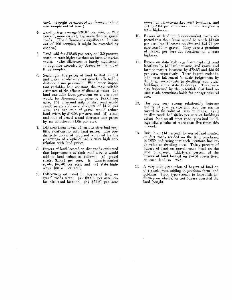
Table 1 SUMMARY OF FINDINGS,

ELLIS COUNTY STUDY

Average Price per Acre of: Land on Dirt Roads Land on Gravel Roads Land on Farm-to-Market Roads Land on Other State Highways

Discount in Price per Acre of Average Land: One Mile from Pavement on Dirt Roads Two Miles from Pavement on Dirt Roads One Mile from Pavement on Gravel Roads Two Miles from Pavement on Gravel Roads

Estimates of Buyers of Land on Dirt Roads: Value per Acre Added by Gravel Roads Value per Acre Added by Farm-to-Market Roads Value per Acre Added by Other State Highways

Estimates of Buyers of Land on Gravel Roads: Value per Acre Discounted for Dirt Roads Value per Acre Added by Farm-to-Market Roads Value per Acre Added by Other State Highways

Estimates of Buyers of Land on Farm-to-Market Roads: Value per Acre Discounted for Dirt Roads Value per Acre Discounted for Gravel Roads Value per Acre Added by Other State Highways

Estimates of Buyers of Land on Other State Highways: Value per Acre Discounted for Dirt Roads Value per Acre Discounted for Gravel Roads Value per Acre Discounted for Farm-to-Market Roads

Value of Buildings per Acre of Land Located on: Dirt Roads Gravel Roads Farm-to-Market Roads Other State Highways

Percent of Buyers Residing on Land Purchased: Buyers of Land on Dirt Roads Buyers of Land on G'I'avel Roads Buyers of Land on Farm-to-Market Roads Buyers of Land on Other State Highways

$ 96.71 138.37 150.36 168.44

$ 22.61 24.31 14.08 15.14

$ 15.71 40.48 81.78

$ 29.30 21.21 33.84

$ 47.50 21.21 21.61

$ 102.54 72.85 38.56

$ 5.24 28.15 33.24 42.69

14% 30 36 36

cant. It might be exceeded by chance in about one sample out of four.)

4. Land prices average $30.07 per acre, or 21.7 percent, more on state highways than on gravel roads. (The difference is significant. In nine out of 100 samples, it might he exceeded by chance.)

5. Land sold for $18.08 per acre, or 12.0 percent, more on state highways than on farm-to-market roads. (The difference is barely significant. It might he exceeded by chance in one out of three samples.)

6. Seemingly, the prices of land located on dirt and gravel roads were not greatly affected by distance from pavement. With other impor­tant variables held constant, the most reliable estimates of the effects of distance were: (a) land one mile from pavement on a dirt road would be discounted in price by $22.61 per acre, (b) a second mile of dirt road would result in an additional discount of $1.70 per acre, (c) one mile of gravel would reduce land prices by $14.08 per acre, and (d) a sec­ond mile of gravel would decrease land prices by an additional $1.06 per acre.

7. Distance from towns of various sizes had very little relationship with land prices. The pro­ductivity index of cropland weighted by the percentage of cropland had a very high cor­relation with land prices.

8. Buyers of land located on dirt roads estimated that improvement of their road service would add to land values as follows: (a) gravel roads, $15. 7l per acre, (b) farm-to-market roads, $40.48 per acre, and (c) state high­ways, $81.78 per acre.

9. Differences estimated by buyers of land on gravel roads were: (a) $29.30 per acre less for dirt road location, (b) $21.21 per acre

more for farm-to-market road locations, and (c) $33.84 per acre more if land were on a state highway.

10. Buyers of land on farm-to-market roads ex­pected that their farms would be worth $47.50 per acre less if located on dirt and $21.21 per acre less if on gravel. They gave a premium of $21.61 per acre for locations on a state highway.

ll. Buyers on state highways discounted dirt road locations by $102.54 per acre, and gravel and farm-to-market locations by $72.85 and $38.56 per acre, respectively. These buyers undoubt­edly were influenced in their judgements by the large investments in dwellings and other buildings along state highways. They were also impressed by the potentials that land on such roads sometimes holds for nonagricultural uses.

12. The only very strong relationship between quality of road service and land use was in regard to the value of farm buildings. Land on dirt roads had $5.24 per acre of buildings value: land on all other road types had build­ings with a value of more than five times this amount.

13. Only three (14 percent) buyers of land located on dirt roads resided on the land purchased in 1959, indicating that such locations had lit­tle value as dwelling sites. Thirty percent of buyers of land on gravel roads lived on the land purchased. Thirty-six percent of the buyers of land located on paved roads lived on such land in 1959.

14. A very high proportion of buyers of land on dirt roads were adding to previous farm land holdings. Road type seemed to have little in­fluence on whether or not buyers operated the land bought.

FARM LAND VALUES AND RURAL ROAD SERVICE IN ELLIS COUNTY, TEXAS, 1955-58

Introduction It is common knowledge that road improvements

stand to reduce the costs and time of travel and increase the freedom of movement of persons and goods. This is the function of transportation and it is the basic pur­pose for which roads are built. It also is understood perhaps that an improvement in road service may en­hance the usefulness and thus the value of the land served. The better the road service available to a tract of land the better will be the relative location of the land. For agricultural land as well as land in other uses improved road service may lead to lower production costs and also to increased marketing efficiencies. Such advantages in turn give rise to larger profits (or margins) which pre­sumably may be reflected in higher land values. Also, through improved location land could be made suitable for a higher and better use and thus would be more valuable. Agricultural land, for example, might become suited for residential or commercial use.

t

In the light of these generally-accepted principles, why then should the effects of various types of roads upon the use and value of land be an important topic of research? First, there is a vital need for such informa­tion, the applications of which will be reviewed momen­tarily. Second, insufficient factual data has been devel­oped on the subject. The economic impact of urban roads has received some study in recent years but there is a distinct shortage of factual information available on road effects in rural areas.

Perhaps the most pressing needs for research re­sults on road effects are in the areas of the economic justification for road improvements, highway finance, and right of way acquisition. Certainly, there may be other applications, as in real estate appraising and taxa­tion and in the over-all planning and programming of economic areas and of road systems, as examples. lnfor-

EACH DOT REPRESENTS A FARM SALE AND THE APPROXIMATE LOCATION OF THE PROPERTY.

COUNTY BOUNDARY

CITY LIMIT

RAILROAD 6t STATION

PRIMITIVE ROAD

~~~8~8 5~~I~NERDO~DOAO SOIL SUR FACE ROAD

METAL SURFACED ROAD BITUMINOUS SURFACED ROAD

PAVED ROAD

ROAD IN CITY Oft INSET

=9!i)== U.S. NUMBERED !'liGHWAY '=(]D= STATE HIGHWAY

~

ELLIS COUNTY TEXAS

FARM OR RANCH TO MARKET ROAD

PAGE SEVEN

mation on road effects also may have implications for road locations, although this may be of less consequence in rural as compared to urban areas.

The problem of the economic justification of road improvements, especially those in rural areas, is a diffi­cult one. Briefly, what must be considered is whether the benefits of a road or roads outweigh the costs of the improvements. Of course, many roads serve rural lands only incidentally. They were built primarily for another purpose, that being to connect urban areas. The use of these roads in the supplying of farms and ranches and in the marketing of agricultural products represents bene­fits to society and to individuals as well. Such benefits which are sometimes measured in ton-miles, vehicular miles and vehicular savings may be added to the other benefits of these truck highways.

The purely rural or land service road yields bene­fits not easily measured by the conventional accounting of vehicular savin~s. Some rural roads remind one of the old story which relates how the outcome of a battle was changed because of the lack of a horseshoe nail. Of small value in itself, a horseshoe nail was shown to have been the critical factor leading to a series of events which resulted in the loss of a battle. Similarly, the value of transportation over many rural roads might seem to be very small if measured by vehicular benefits. In view of the fact that such transportation may be criti­cal to the commerce of the nation, however, the problem of justification changes in perspective. The benefits of a road involve the final and total implications and conse­quences of the road and these may be diffused in many ways and to many places.

The fact that variations in road service may be re­flected in land values presents another opportunity for the measurement of road benefits. Differentials in land value due to differentials in road service do not include all road benefits. Actually, the effects of roads on land values might be considered as measurements of only a portion of vehicular benefits. Since land value benefits are not separate and apart from other types of benefits, care must be taken in considering them to avoid double­counting in benefit-cost analysis. Nevertheless, the im­pact of road improvements on the value of land should

PAGE EIGHT

not be disregarded and may be useful in the economic justification of highway construction.

In regard to highway finance, the sharing of the costs of roads should not be decided without regard to the identity of the beneficiaries. Road users have borne most of the burden of road costs and road users are primary beneficiaries. But if some road benefits accrue to land, and road users are not necessarily the same persons who own the land, then the question of equity becomes apparent. It is not suggested that landowners whose property is enhanced by roads should pay a part of the cost of roads. Historically such windfalls remain with those who receive them except in cases where capi­tal gains and increased values are recognized in income or ad valorem tax payments. It may be suggested, how­ever, that benefits of all kinds should be weighed in con­siderations of highway finance.

One of the most promising applications of informa­tion on road effects is in the field of right of way acqui­SitiOn. In all cases where a part of a property is to be acquired, knowledge of the possible consequences of the new road will improve the chances for a quick and equitable settlement. The payment of excessive damages may be avoided if factual histories of the influences of road improvements are available. Such information also may be of utility in the location and design of roadways.

This particular study of the effects of various road types on farm land values in Ellis County, Texas, was conducted under a cooperative arrangement with the United States Bureau of Public Roads. Its first purpose is to contribute to the section on nonvehicular benefits of roads in the Bureau's report to Congress in early 1961.

Like previous studies of the economic impact of rural roads, the study is in many ways exploratory and incomplete. The report emphasizes land values as affect­ed by four general road types, these being dirt, gravel, farm-to-market roads and state highways. The land value measurements are based both upon land sales and buyers' estimates of road effects. Very little information was developed in the study on the influence of road types on land use, although the topic does receive some attention in the report.

Characteristics of Ellis County Ellis County is located in the North Central part of

Texas in an area known generally as the "Blacklands" or the Blackland Prairie. It was settled early in Texas history, having been created about 1850. It is bordered on the North by the Dallas and Fort Worth metropolitan areas and in recent years has been influenced a great deal by their nearness. In the 1960 census of popula­tion, Ellis County will be included for the first time as a part of the Dallas metropolitan area. Yet, the county retains many of its rural characteristics.

Ellis County has an area of 953 square miles, and despite its many towns and villages, this land area is used predominantly for agriculture. Its population density in 1950 was less than 50 persons per square mile. It is probable that this figure had not changed a great deal by 1960.

Interstate Highway 35 East is to be located through the center of the county, serving the county seat, Waxa­hachie, and other points. IH 45 is being located on the east side of Ellis County and serves several of the coun­ty's towns and villages.

Population and Employment

Table 2 reviews several of the population and em­ployment characteristics of Ellis County in 1950. These data, of course, are quite out-of-date and several impor­tant changes will be demonstrated in the 1960 census of population. Perhaps the 1950 figures, however, are use­ful for describing the general nature of the county in comparison with Texas' population and employment. It may be noted also that these data apply to a period only five years prior to the first year for which farm sales were observed in the study.

From the standpoint of population, Ellis County still was predominantly rural in 1950. Of the 45,645 total population, 58.3 percent were classified as rural. Texas, in contrast, had only 37.3 percent rural population in 1950. The proportion of rural farm population in the county was 31.7 percent compared with 16.8 percent for the State.

Farm employment also made up a much larger pro­portion of total employment in Ellis County than in the

'!'able 2 POPULATION AND EMPLOYMENT ELLIS COUNTY AND TEXAS, 1950*

Total Population Percent Urban Percent Rural Percent Rural Nonfarm Percent Rural Farm

Total Employment Percent Nonfarm Percent Farm Percent Farmers and

Farm Managers Percent Other Farm

Ellis County

45,645 41.7 58.3 26.6 31.7

15,928 71.3 28.7

17.0 11.7

Texas

7,711,194 62.7 37.3 20.5 16.8

2,758,443 84.6 15.4

9.1 6.3

*Source: United States Census of Population: 1950. Volume II, Part 43, Chapter B.

State as a whole. The figures were 28.7 percent for Ellis County and 15.4 percent for Texas.

The five largest towns of the county are listed below with their 1950 populations. (These data are from the source given in Table 2.)

Waxahachie ____________ 11,204 Ennis _________________ 7,815 Ferris _________________ 1, 735 Italy __________________ 1,185 Midlothian ____________ 1,177

One source estimates that the population of W axa­hachie had grown to 14,000 by 1957 (Texas Almanac, 1958-59, A. H. Belo Corp., Dallas). Later estimates were not obtain.ed for the other towns listed.

Out-of-county population centers which draw trade and also furnish employment for some Ellis Countians are as follows:

Dallas-about 800,000 in population in 1960 and about 20 miles from the Ellis County line.

Fort Worth-more than 500,000 population in 1960 and about 25 miles from Ellis County.

Waco-more than 100,000 population in 1960 and roughly 44 miles away.

Corsicana-perhaps 25,000 in population in 1960 and about 12 miles from the Ellis County line.

Hillsboro-with a 1960 population of about 10,000, and 12 miles from the nearest point in Ellis County.

Farm Characteristics

Many years ago Ellis County was the leading cot­ton producer among the counties of Texas. Its average rainfall of 35 inches per year and its natively fertile black waxy soils were conducive to good yields accompa­nied by relatively low costs of production. Long before acreage controls, however, cotton production began to decrease in importance relative to small grain and cattle enterprises. Yet, in 1960 cotton still was the county's more important agricultural commodity and probably will remain so for some time. The production of grain

Table 3 FARM CHARACTERISTICS

ELLIS COUNTY AND TEXAS, 1954*

Number of Farms Average Size (Acres) Percent of Farms Commercial Percent of Farms Part-Time Percent of Farm Tenancy Percent of Farms With

Operator-Resident Land in Farms (Acres) Percent of Land in Cropland Percent of Land Pastured Percent of Land in Woodland

Ellis County

2,885 192.6 75.2 17.0 47.0

85.5 555,526

72.7 35.3

3.1

Texas

292,947 498

62.3 15.6 25.9

86.8 145,812,733

25.1 77.8 13.7

*Source: United States Census of Agriculture: 1954. Volume I, Part 26, Texas.

PAGE NINE

sorghum, corn, and beef cattle are activities of growing importance. Bee-keeping, dairying and some truck crop­ping also add to farm income.

Table 3 lists some additional farm characteristics of Ellis County with comparisons with the State. In 1954, Ellis County had 2,885 farms which averaged about 193 acres in size, less than half the average size of Texas' farms. About three-fourths of the Ellis County farms were rated as commercial, a greater proportion than for the State.

Evidence that the county was predominantly a farm­ing rather than a livestock producing area is seen in the proportion of cropland. About 73 percent of the land in farms in Ellis County was in cropland in 1954 com­pared to about 25 percent for Texas. It is not likely that these data would have changed much by 1960.

Ellis County had a higher tenancy rate than Texas. A rather high proportion of farms had operator-residents in both the county and the State. It is likely that this proportion has decreased in recent years. It seems prob­able also that part-time farming has increased from the 17 percent level in Ellis County in 1954.

The rather high proportions of cropland, operator­residents and part-time farmers suggests that Ellis Coun­ty's farms are quite dependent upon motor vehicles and thus good roads for successful operation.

Road Facilities The construction of farm-to-market roads at a rapid

pace quickly out-dates information such as that presented in Table 4. If such data were available for a later time than 1950, some very important changes probably would be revealed. However, in 1960, Ellis County still had a great deal of variation in the quality of rural road serv­ice and a look at the 1950 situation is not too misleading.

In 1950, 27.4 percent of the county's farms were located on paved roads. In the study of 1955-58 farm land sales, about 37 percent of the tracts which sold were found to be on paved roads. Figures for 1950 show

PAGE TEN

43.6 percent of farms to have been on gravel roads. The 1950 census data show that 29 percent of Ellis County farms were on dirt roads. (Of farms which sold during 1955-58, 43 percent were on gravel roads, 0.2 of a mile or more from pavement and 20 percent were on dirt roads.)

It is interesting that the average distance of farms on dirt roads, as observed in the study of sales, was 0.81 of a mile. In 1950, the average distance from all Ellis County farms over dirt roads to the trade center visited most frequently was 0.9 miles. The figures of 0.81 and 0.9 miles measure different road service characteristics but their similarity is worthy of note. It is suggestive, along with the other comparisons, that farms which sold in Ellis County during 1955-58 had road service ver.y much like that of all Ellis County farms.

It might be mentioned that Ellis County apparently had somewhat better road facilities in rural areas in 1950 than did the rest of Texas. The State had a slightly higher proportion of farms on paved roads, but nearly half of its farms were located on dirt roads. Ellis Coun­ty, comparatively, had a rather high percentage of its farms served by gravel roads.

Table 4 ROAD FACILITIES OF FARMS

ELLIS COUNTY AND 'I'EXAS, 1950*

Ellis County

Kind of Road: Number of Farms Reporting Hard Surfaced, Percent Gravel (Shell or Shale), Percent Dirt or Unimproved, Percent

Distance Over Dirt or Unimproved Roads to Trading Center Visited Most Frequently:

Number of Farms Reporting 0.0 to 0.2 Miles, Percent 0.3 to 0.9 Miles, Percent 1.0 to 4.9 Miles, Percent 5.0 and Over Percent Average Distance, Miles

3,158 27.4 43.6 29.0

2,984 60.5 10.3 23.3

5.9 0.9

*Source: United States Census of Agriculture: Volume I, Part 26, Texas.

Texas

313,097 30.7 19.8 49.5

288,044 38.5 9.8

36.7 15.0 2.1

1950.

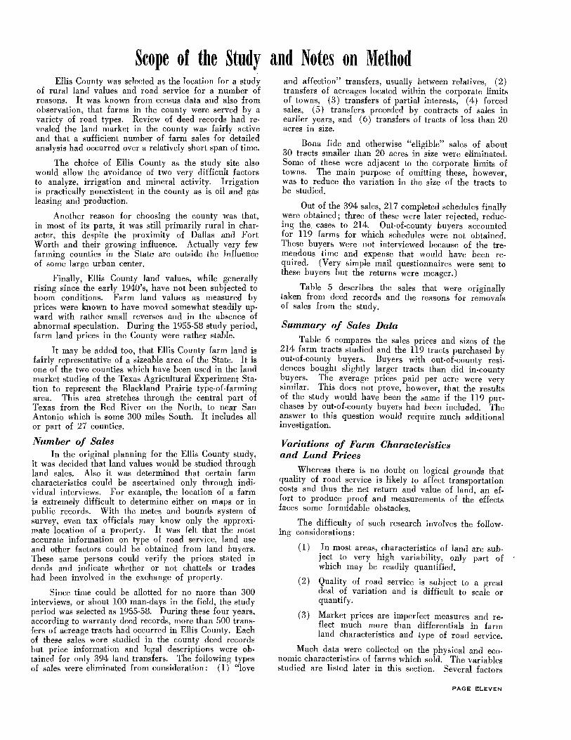
Scope of the Study and Notes on Method Ellis County was selected as the location for a study

of rural land values and road service for a number of reasons. It was known from census data and also from observation, that farms in the county were served by a variety of road types. Review of deed records had re­vealed the land market in the county was fairly active and that a sufficient number of farm sales for detailed analysis had occurred over a relatively short span of time.

The choice of Ellis County as the study site also would allow the avoidance of two very difficult factors to analyze, irrigation and mineral activity. Irrigation is practically nonexistent in the county as is oil and gas leasing and production.

Another reason for choosing the county was that, in most of its parts, it was still primarily rural in char· acter, this despite the proximity of Dallas and Fort Worth and their growing influence. Actually very few farming counties in the State are outside the influence of some large urban center.

Finally, Ellis County land values, while generally rising since the early 1940's, have not been subjected to boom conditions. Farm land values as measured by prices were known to have moved somewhat steadily up­ward with rather small reverses and in the absence of abnormal speculation. During the 1955-58 study period, farm land prices in the County were rather stable.

It may be added too, that Ellis County farm land is fairly representative of a sizeable area of the State. It is one of the two counties which have been used in the land market studies of the Texas Agricultural Experiment Sta· tion to represent the Blackland Prairie type-of-farming area. This area stretches through the central part of Texas from the Red River on the North, to near San Antonio which is some 300 miles South. It includes all or part of 27 counties.

Number of Sales In the original planning for the Ellis County study,

it was decided that land values would be studied through land sales. Also it was determined that certain farm characteristics could be ascertained only through indi­vidual interviews. For example, the location of a farm is extremely difficult to determine either on maps or in public records. With the metes and bounds system of survey, even tax officials may know only the approxi­mate location of a property. It was felt that the most accurate information on type of road service, land use and other factors could be obtained from land buyers. These same persons could verify the prices stated in deeds and indicate whether or not chattels or trades had been involved in the exchange of property.

Since time could be allotted for no more than 300 interviews, or about 100 man-days in the field, the study period was selected as 1955-58. During these four years, according to warranty deed records, more than 500 trans­fers of acreage tracts had occurred in Ellis County. Each of these sales were studied in the county deed records but price information and legal descriptions were ob­tained for only 394 land transfers. The following types of sales were eliminated from consideration: ( l) "love

and affection" transfers, usually between relatives, (2) transfers of acreages located within the corporate limits of towns, ( 3) transfers of partial interests, ( 4) forced sales, ( 5) transfers preceded by contracts of sales in earlier years, and ( 6) transfers of tracts of less than 20 acres in size.

Bona fide and otherwise "eligible" sales of about 30 tracts smaller than 20 acres in size were eliminated. Some of these were adjacent to the corporate limits of towns. The main purpose of omitting these, however, was to reduce the variation in the size of the tracts to be studied.

Out of the 394 sales, 217 completed schedules finally were obtained; three of these were later rejected, reduc­ing the. cases to 214. Out-of-county buyers accounted for 119 farms for which schedules were not obtained. These buyers were not interviewed because of the tre· mendous time and expense that would have been re­quired. (Very simple mail questionnaires were sent to these buyers but the returns were meager.)

Table 5 describes the sales that were originally taken from deed records and the reasons for removals of sales from the study.

Summary of Sales Data

Table 6 compares the sales prices and sizes of the 214 farm tracts studied and the 119 tracts purchased by out-of-county buyers. Buyers with out-of-county resi­dences bought slightly larger tracts than did in-county buyers. The average prices paid per acre were very similar. This does not prove, however, that the results of the study would have been the same if the 119 pur­chases by out-of-county buyers had been included. The answer to this question would require much additional investigation.

Variations of Farm Characteristics and Land Prices

Whereas there is no doubt on logical grounds that quality of road service is likely to affect transportation costs and thus the net return and value of land, an ef­fort to produce proof and measurements of the effects faces some formidable obstacles.

The difficulty of such research involves the follow­ing considerations:

( l) In most areas, characteristics of land are sub­ject to very high variability, only part of which may be readily quantified.

(2) Quality of road service is subject to a great deal of variation and is difficult to scale or quantify.

( 3) Market prices are imperfect measures and re· flect much more than differentials in farm land characteristics and type of road service.

Much data were collected on the physical and eco­nomic characteristics of farms which sold. The variables studied are listed later in this section. Several factors

PAGE ELEVEN

Table 5 NUMBER OF 1955-58 FARM SALES, ELLIS COUNTY,

AND REASONS FOR OMITTING SALES FROM THE STUDY

Number of farm sales recorded from deed records 394 Records indicated buyer lived outside of county;

no attempt was made to interview these 90

Number of attempted interviews 304 Completed schedules 217

Sales for which interviews were not obtained* 87

*These schedules were not completed because: Additional buyers found to be out-of-county

residents 29 Buyer claimed sale not bona fide 29 Multiple purchaser (one person bought 16

tracts, interview covered only 4 tracts) 12 Farm purchased for residential development 7 Refusals 3 Resales of land 7

not studied were slope of land, nature of water supply, type of financing and a number of qualitative attributes which possibly would explain value differentials.

Road service characteristics were described to buy­ers in rather simple terms. Only the most·commonly known road types were determined, these being dirt, gravel, farm-to-market and other state highways. Farm­to-market roads are state-built roads of excellent design; they allow safe speeds of 45 to 50 miles per hour, have 20 feet of treated surface and have bridges of a 30,000 pound capacity. Some county roads having bituminous surfacing were included as farm-to-market roads but these were few in number. "Other state highways" re· fers to state-numbered roads other than farm-to·market.

The only other quantification of type of road serv­ice was distance of farms from paved roads. This varia­ble was used in relation to dirt and gravel roads only, of course.

The type of public road at or within 0.2 mile of the usual place of entry to a tract was used as the type of road location of the land. The use of the 0.2 mile requirement eliminated a number of "borderline" cases where superior road service was very close.

Ideally, any differences within road types would be observed and measured. Bridges on dirt and gravel roads vary a great deal in width and load limits. Also some dirt roads may be superior to the poorest of gravel

Table 6 SUMMARY OF SALES DATA FOR 214 FARMS STUD­IED AND FOR 119 FARMS PURCHASED BY OUT OF

COUNTY BUYERS, ELLIS COUNTY, 1955-58

Number of Sales Acres Purchased Total Price Paid Average Price Per Farm Average Acres Per Farm Average Price Per Acre*

*Area weighted.

PAGE TWELVE

Useable Out of County S h Buyers

c edules (Not Interviewed)

214 22,104

$2,918,504 $13,638

103 $132

119 15,560

$2,053,920 $17,260

130 $133

A very common type of dirt road in Ellis County.

roads for very long periods of time; the only advantage of gravel might be that it is generally passable through­out the year. The problem, however, of quantifying road characteristics and distance for individual farms is so complex that additional refinements would require much time and expense.

A very large proportion of the variation in land prices may be accounted for by the imperfections of the land market. One buyer for example who paid $18,500 for a tract reported that he would have paid as much as $23,000. On the other hand, this same tract had been offered for several months at or very near the actual

A county-maintained gravel road.

A farm-to-market road; asphalt surface, built and main­tained by the State.

selling price. Lack of knowledge, not only of buying and selling opportunities but of value ranges and trends, is a dominant factor in the land market. Also, basic productivity is often ignored. The availability of financ­ing varies from area to area, from farm to farm, and over time, and is reflected in exchange prices. The needs of some buyers and sellers may be more urgent than those of other buyers and sellers. Some buyers are willing to pay for the aesthetics such as an attractive landscape. Other buyers are seeking residential sites, perhaps for the distant future. Some buyers are willing to pay the replacement value for buildings, others con­sider buildings to be a liability. A market transaction may reflect the proportion of cropland or this charac­teristic may be ignored and a premium put on improved pasture land. The income tax positions of both buyer and seller may influence the exchange price of individual tracts and also the terms of the purchase.

To some extent land prices are likely to be related to the yields of the land during the previous year and to a one-year outlook. For example, a farm with very good crop prospects in the spring may sell for dispro­portionately more than the same farm with a dismal harvest some months later. Additional characteristics, which affect farm land value but perhaps imperfectly, are the presence of noxious weeds, the state of repair of fences, the apparent supply of water and the quality of conservation structures.

Many of these and other physical attributes of farms as well may be observed and quantified. Generally the process, to be adequate, would require an exhaustive case study and appraisal of each farm's resources. And then if the exchange price was faulty for reasons not determined, perhaps institutional reasons, the objective of asceriaining the contribution of each factor to land price still would not be accomplished. Yet another com­plicating factor is the fact that many variables are re­lated and act jointly on price, at least theoretically.

Methods of Analysis

Whereas any of several treatments of the data may have been appropriate, only cross-classification and mul­tiple regression analyses were attempted. The problem, simply stated, was to test the hypothesis that land values varied with quality of road service. Although the farm sales analyzed occurred over a four-year span, no effect of time was isolated or observed. Thus sales were treated as if they had occurred simultaneously.

Cross-classification analyses were made on a very limited scale because of the number of observations. The 214 sales (and an even smaller number of buyer esti­mates) very quickly resulted in small-frequency or empty cells when classified by two or more criteria.

For this reason, attention soon was turned to multi­ple regression analysis. This method would allow in­terpolated answers which were not provided by cross­classification. The next section discusses the factors con­sidered and something of the problems met in regression analysis.

Variables Considered in Regression Analyses

At one point or another in the calculations more than 30 different variables were considered in attempts to isolate road service effects on land values within a meaningful framework. Many factors were eliminated because of their very high correlation with other factors. In other words, as would be expected, two or more fac­tors might measure the same basic land characteristic. A notable example of this was that net rent per acre (based on collected rents and landlords' customary shares) was highly correlated with the productivity index of cropland and both factors were significantly corre­lated with land prices. The following is a list of the various factors that received attention; some of these were entered into calculations in several forms. Sources of the information are given in parenthesis.

l. Price paid for land (from warranty deed rec-ords; verified by buyer) .

2. Year of purchase (deed records and buyers) .

3. Acreage purchased (deed records and buyers) .

4. Distance on dirt to nearest paved or gravel road (maps and buyers).

5. Distance on gravel to nearest paved road (maps and buyers) .

6. Distance to usual place of shopping (maps and buyers).

7. Distance to usual place of marketing (maps and buyers).

8. Cropland productivity index (USDA records, ASC).

9. Averaze annual net rent, 1955-58 (buyers).

10. Percent cropland (buyers).

11. Percent cotton allotment (buyers and ASC rec­ords).

12. Percent cotton acreage (buyers).

13. Value of buildings (buyers' and researchers' estimates) .

PAGE THIRTEEN

14. Distance to nearest large trade center (maps and buyers).

15. Distance to nearest smaller trade center having a school (maps and buyers) .

16. Percent pasture (buyers).

17. Grazing capacity of pasture (buyers).

18. Distance to Dallas (maps).

19. Average cotton yield, 1955-58 (buyers).

20. Distance via farm-to-market road to nearest large town (maps).

21. Distance via state highway to nearest large town (maps).

22. Product of 4 and 13.

23. Product of 8 and 10.

24. Product of 12 and 19.

25. Product of 16 and 17.

26. Logarithms of several factors.

27. Sums of various distance factors.

Several of the factors listed require special expla­nation. The cropland productivity index, Item 8 above, is that measurement assigned to particular tracts by the County Committee for Agricultural Stabilization and Conservation. This duty was guided by Paragraph 153 of USDA Manual 1-SB. The instructions require in part that "the indexes fairly represent the relative productivity of the farms." Average cropland for Ellis County would have an index of 100. To be considered in the determi­nation of the index numbers were: "1. Available yield data, including data furnished by the farmer. 2. Land classification suitability data. 3. Soil survey informa­tion." The resultant ASC index was correlated with land prices (r=.22) but also, as would be expected, it had a high correlation (r=.59) with percentage of cropland. The product of these two factors therefore was obtained (Item 23) and is referred to in this report as the pro­ductivity index, which may be considered a measure of the average of all acres in a tract from the standpoint of cropland productivity.

Item 13, the value of buildings, was sought through both buyers' and researchers' estimates. Interviewers were instructed to try to estimate the replacement costs (new) of all buildings. They further were given direc­tions on how to estimate current condition, accrued main­tenance and the functional characteristics of buildings. All of the factors were then considered to obtain an "appraised" value.

Buyers had a great deal of difficulty in assessing building values; finally they were asked to estimate what they would have been willing to pay for the land if it had not had buildings. Buyers' and researchers' esti­mates were correlated (r=.62) but neither measure seemed to be sufficient alone. Therefore, a combination of the two was made in the following manner: The buyer's estimate was taken if it exceeded that of the re­searcher. The average of the two estimates was used if the researchers' estimate was the larger. These judge­ments were made because it was fairly obvious that the researchers tended to overestimate building values, whereas buyers seemed to be conservative.

PAGE FOURTEEN

In reference to Items 14 and 15, "large trade cen­ter" was defined as a town or city which would serve most of the social and economic requirements of farm tracts and farm families and a "small trade center" was a town having a school. Such small towns had been determined as also having a bank, a gin and one or more stores and other services.

Item 17, grazing capacity of pasture, was the buy­er's estimate of the acres of pasture required to sustain a cow or cow-equivalent in the usual cow-calf enterprise. Yield data such as used for Item 19 was the average of annual yields as recalled for individual years by the land buyers.

Bridge scenes on a State highway and on a gravel road.

The large and small towns referred to in Items 20 and 21 were identical to the trade centers in Items 14 and 15 respectively.

After the first matrix of simple relationships was inspected, a large number of the variables were elim­inated from further study. Table 7 presents the simple relationships between the variables which were retained for continuing use in subsequent estimating equations. The factors were tried in logarithmic form and also as natural numbers. Several other curvilinear fits were attempted.

A deletion process was used for each equation form which was tested. Following each solution, the weakest variable from the standpoint of the coefficient-standard error ratio was deleted, assuming that the ratio was 1.96 or less (equivalent to 95 percent confidence level.) After the deletion, another solution was obtained. Again the variable with the smallest coefficient-standard error ratio was dropped. This process was continued until only factors statistically significant (according to the ratio test) were retained. The program for these solutions was prepared by the Data Processing Center, Texas A & M College and the IBM 650 was used for calculations.

Table 7

SIMPLE RELATIONSHIPS* BE'I'WEEN VARIOUS FACTORS, 214 ELLIS COUNTY FARMS WHICH

SOLD DURING 1955-58

Factor Yx1x,x,x.x,x.

Y = Price per acre X1 = Distance on

1.00 -.26 -.14 .54 .35 -.09 -.15

dirt road X, = Distance on

gravel road X, = Buildings value

per acre X. = Productivity index X, = Distance to nearest

large town X. = Distance to nearest

small town

1.00 .00 -.22 -.12 .17 .06

1.00 -.07 -.05 .31 .11

1.00 .01 -.14 -.09 1.00 .23 -.10

1.00 .00

1.00

*Simple correlation coefficients.

Time after time the only variables which survived this rigorous test were the value-of-buildings factor and the productivity-index factor. Because of the objectives of the study, the "best" solution for each estimating equation finally was taken as that which retained the road service factors which were to be evaluated and all factors whose coefficient-standard error ratio was at least as great as that of the road factors. In other words, the desired road factors and other factors which were as statistically significant were retained. Of course, cer­tain logical tests also were kept in mind; coefficients were required to be positive or negative as would be compatible with the rationale. For example, if the pro­ductivity-index factor carried a negative sign in the pres­ence of certain other factors, the solution was rejected. Then another estimating equation was attempted after study of the interrelationships.

Most equations which were attempted explained about 40 percent of the total variation in prices (accord­ing to the square of the corrected coefficient of multiple regression). It is also worthy of note that coefficients for X1, distance from pavement on dirt roads, and X2,

distance from pavement on gravel roads, fell into relative narrow ranges under the various solutions. Of course, it should be realized that the equations did not vary greatly, there being three or more factors (in some form) common to all equations.

It is felt that perhaps the best approach to road service evaluation is to develop four regression solutions, one each for dirt, gravel, farm-to-market and state high­way locations. One solution of this nature was attempted but did not contribute to the understanding of the rela­ionships. Such an approach usually requires a far larg­er number of observations than were used in the Ellis County study.

A great many further trials might have been made in an attempt to explain land prices observed in Ellis County. Some very interesting variables not fully con­sidered were distance of the farm to Dallas, pasture land quality, and several products of two or more factors. Interaction of variables apparently was present but ef­forts to demonstrate and measure such relationships gen­erally were not fruitful.

PAGE FIFTEEN

Analysis of Land Prices A very large number of factors influences the mar­

ket price of farm land. Basic productivity of the land, value of buildings and other improvements, and the lo­cational characteristics of a particular farm obviously should have an important bearing on the price the farm will command in relation to other farms. Such factors were considered in the analysis of land prices.

There are other factors which affect land prices in general; examples are commodity prices, costs of labor and equipment and availability and costs of mortgage financing. However, changes in such factors may affect farm land prices differentially as well as in general. Low quality land may rise proportionately more in price than better quality land when farm commodity prices increase. In Ellis County, a rise in the price of cotton is likely to increase the price of farms having cotton acreage allot­ments more than farms not having allotments. Neverthe­less, in the Ellis County study these latter factors were generally omitted in the analysis of land prices and type of road service. The omission is justified on the follow­ing grounds:

( 1) The farm land sales observed were over a relatively short period of time, 1955 to 1958, during which commodity prices and produc­tion cost changes were relatively small, the exception being increases in cattle prices.

AVERAGE PRICE PER ACRE FOR FARMS ON EACH TYPE ROAD

18 0

160

140

120

<fl I 00 Q:

<t ..J ..J 0 0 80

60

40

20

PAGE SIXTEEN

DIRT ROADS

(2) Preliminary study indicated that farms on the various road types were not greatly different from the standpoint of land use. An excep­tion to this had to do with value of buildings.

(3) It was felt that many adjustments that might be attempted in data for individual farms would be hazardous as to results, this even if a detailed farm management analysis were made for each farm.

The following analysis therefore involves only four factors: (a) land prices, (b) type of road location and distance from pavement, (c) value of buildings per acre, and (d) the productivity index of the land. (The latter variable was the ASC cropland productivity index weighted by the percent of cropland. When introduced into multiple regression equations, it was found to have a highly significant influence on land values.)

Average Prices Per Acre of Land on Various Road Types

In the Ellis County study, 214 sales of farm land were analyzed in an attempt to determine the effect of type-of-road location on farm land prices. The results of one of the first calculations are shown in Table 8. Without regard to the many ways in which farm land varies in character, the average prices of land along the four road types showed an expected pattern.

Farms on dirt roads (0.2 of a mile or more from gravel or pavement at the usual place of entry) sold for an average of $96. 7l per acre or 71 percent of the aver­age price for all 214 farms. Farms located on gravel roads ( 0.2 mile or more from pavement) had an average price of $138.37 per acre.

The average price on farm-to-market roads was $150.36 per acre, while farms on other state highways brought a still higher price-$168.44 per acre. The na­ture of the differences in prices is explored further in Table 8.

Land on gravel roads sold for $41.66 per acre, or 43.1 percent, more than did land on dirt roads. The confidence level given in Table 9 may be explained as follows: Assuming sales of land on dirt roads and gravel

Table 8

AVERAGE SALES PRICES PER ACRE OF 214 FARMS LOCATED ON VARIOUS ROAD TYPES

ELLIS COUNTY, 1955-58

Type of Road Number of Farms

Dirt 42 Gravel 92 Farm-to-Market 64 Other State Highway 16 All Farms 214

*Not area weighted.

Average Price

Per Acre*

$ 96.71 138.37 150.36 168.44 136.03

Percent of Average

Price Per Acre, All Farms

71 102 111 124 100

roads to be samples, the probability is only one in 100 that a greater difference than $41.66 per acre might be found because of sampling error in successive samples. Thus it may be said with a 99 percent probability of being correct that there is a real difference between values of land on dirt versus gravel roads. This is to say, the $41.65 difference is highly significant.

Land prices on farm-to-market and other state roads also were significantly greater than those on dirt roads. The differences are accompanied by 99 percent confi­dence levels.

It may be inferred that the improvement of road locations from gravel to farm-to-market, from gravel to other state highway and from farm-to-market to other state highway would be accompanied by land price in­creases. Statistically, however, the inferences are some­what weak as is reflected by the confidence levels. For example, the probability is only about 2 out of 3 ( 67 percent) that the difference between average prices on farm-to-market roads and other state highways is real rather than a chance occurrence of sampling (sales).

Mutiple Regression Analysis

The information shown in Tables 8 and 9 does not take into account that farms on one type of road may be far different from farms located on other road types. For example, it might be questioned whether better qual­ity land generally has better road service than poorer land. Furthermore, variations in distance from pavement were not considered for locations on dirt and gravel roads.

Table 10 presents the results of calculations which allow for the value of buildings and the productivity index of the various farms. (The equation used was linear in form except that the logarithms of distances on dirt and on gravel were introduced as the distance fac­tors. After the determination of regression coefficients, the logarithms corresponding to various distances were introduced. Transformations were then made to obtain value changes related to distance changes. This process yielded curvilinear relationships for distance from pave­ment and land prices.)

The data presented in Table 10 supports earlier findings that farms on dirt and gravel sell for signifi-

Table 9 DIFFERENCES IN AVERAGE SALES PRICES PER

ACRE OF FARMS LOCATED ON VARIOUS ROAD 'I'YPES ELLIS COUNTY, 1955-58

Differences in Road Type Change Prices Per Acre Confidence

Assumed Dollars Percent Level* Added Added

Dirt to GTavel $ 41.66 43.1 o/o 99% Dirt to Farm-to-Market 53.65 55.5 99 Dirt to Other

State Highway 71.73 74.2 99 Gravel to Farm-to-Market 11.99 8.7 73 Gravel tr> Other

State Highway 30.07 21.7 91 Farm-to-Market to Other

State Highway 18.08 12.0 67

*Based on significance of difference of means.

cantly less than do farms on pavement. A farm located on a dirt road one mile from pavement might be expected to sell for $22.61 per acre, or 14.3 percent, less than a similar farm located on a paved road. Additional miles from pavement, however, would cause much smaller de­creases in value. The second mile of dirt road, for ex­alTiple, would depress land prices by only $1.70 per acre ($24.31 - 22.61) by 1.1 percent (15.4 percent- 14.3 per­cent).

These findings lead to the conclusion that the mere fact that a farm is located on a dirt road causes the ma­jority of the discount in value and that additional dis­tance on dirt is of sharply decreasing importance in land pricing. Two logical explanations of this finding are in order at this point. First, a short distance on dirt may be as much of a deterrent to travel as a longer distance when the road is impassable for motor vehicles.

Second, it was found that only a third of the farms on dirt roads had dwellings and some of these were bare­ly habitable. Thus, locations on dirt roads apparently are accorded little value for residential purposes.

Farms one mile on a gravel road had a discount of $14.08 per acre compared to similar farms located on paved roads. According to the system of analysis used to compile Table 10, additional miles on gravel would cause land prices to decrease but by very small amounts. These findings are not subject to the same explanations offered for dirt road effects. Whereas gravel roads are not strictly all-weather, they become impassable much more seldom and for much shorter periods than do dirt roads. They can be exceedingly rough and dusty but these attributes seemingly would result in greater dis­counts in land values for additional distances than those reported in Table 10.

Table ll shows the results of another analysis of the effects on land values of distance of land from pavement. Again, value of buildin~<s and the productivity index are factors which were held constant in their influences. The findings from this equation show that the first mile

Table 10 INTERPOLATED PRICES PER ACRE OF FARMS LO­

CATED VARYING DISTANCES ON DIRT AND GRAVEL ROADS ELLIS COUNTY, 1955-58

(EQUATION 1)

Type or Road Location and Distance to Pavement

Located on Dirt Road: 1 mile from pavement 2 miles from pavement 3 miles from pavement

Located on Gravel Road: 1 mile from pavement 2 miles from pavement 3 miles from pavement

Located on Paved Road:

Price per Acre and Dollar and Percent Discount

Price per Acre

Average Farm'

$135.25 133.55 132.55

143.78 142.72 142.10 157.86

Discount per Acre•

Dollars Percent

$22.61 14.3% 24.31 15.4 25.31 16.0

14.08 8.9 15.14 9.6 15.76 10.0

'Average farm assumes building value per acre of $26.26 and a productivity index of 70.

"Coefficient for distance on dirt road is significant at 3% level; coefficient for distance on gravel road is significant at 4 o/o level.

PAGE SEVENTEEN

of dirt road would reduce values by $15.78 per acre or 11.1 percent. Each additional mile would also diminish values by $15.78 per acre. (This was the nature of the equation used in the estimate. Distance from pavement was entered into the equation in natural numbers.) It should be emphasized that the results are not as signifi­cant statistically as those reported in Table 10. (This is to say that Equation 2 does not describe the relationship as well as does Equation l.)

According to Equation 2, land one mile from pave­ment on a gravel road would be discounted $5.42 per acre or 3.8 percent. Additional miles would each cause a further discount of $5.42 per acre. Again the results are not as significant statistically as those yielded by Equation 1 as shown in Table 10.

The assumption that each mile of distance from pavement will have the same dollar effect on land prices assumes in turn that transportation costs have a straight­line relationship with distance on unpaved roads. This is to say that. at least in the minds of land buyers and land sellers, the second mile (and each additional mile) of unpaved road causes as much increase in time of travel and motor operating costs as does the first mile. As opposed to this assumption, Equation 1 which yielded the results in Table 10 tests the hypothesis that addi­tional miles of unpaved road will add less and less to transportation costs. Similarly, it suggests that the land market (the action of buyers and sellers) places a stigma on dirt or gravel road locations but places relatively less importance on distance from pavement.

Variations in Values of Buildings on Various Road Types

One of the complicating factors in the determina­tion of land price differentials as related to type of road location was the variation in the value of building from farm to farm. The equations used to compile Tables 10 and 11 included building values as a variable. It was found in the calculations that distance on dirt roads and

'I'able 11 INTERPOLATED PRICES PER ACRE OF FARMS LOCATED VARYING DISTANCES ON DIRT AND

GRAVEL ROADS, ELLIS COUNTY, 1955-58 (EQUATION 2)

Type of Road Location and Other Specified Characteristics

Located on Dirt Road: 1 mile from pavement 2 miles from pavement 3 miles from pavement

Located on Gravel Road: 1 mile from pavement 2 miles from pavement 3 miles from pavement

Located on Paved Road

Price per Acre and Dollar and Percent Discount

Price per Discount per Acre2

Acre Average Dollar Percent Farm'

$125.90 $15.78 11.1% 110.12 31.56 22.2

94.34 47.34 33.3

136.24 5.42 3.8 130.82 10.84 7.6 125.40 16.26 11.4 141.68 0 0

'Average farm assumes building value per acre of $26.26 and productivity of 70 per acre.

"Coefficient for distance on dirt significant at 6% level; coefficient for distance on gravel significant at 8% level.

PAGE: EIGHTEEN

value of buildings were inversely correlated. While this correlation was not great (r = - .22) and is of little significance statistically, it is interesting and might be expected on logical grounds. It is supported by simple tabulations which indicate that the better the road type the greater the value of buildings per acre, from the standpoint of averages.

These findings suggested the treatment presented in Table 12. Here it is shown that farms on dirt roads had a very low $5.42 per acre of estimated building values. Farms on other roads had buildings of more than five times this value; and repeating, the better the road type the greater the value of building per acre. It was decided that perhaps the removal of building values as estimated from total purchase prices would give a fair estimate of what was paid for land only. The resultant prices per acre are shown in Table 12. The ad­justed prices, however, are not as reliable statistically as the unadjusted prices shown in the first column (and also in Table 8.) The statistical significance of the dif­ferences between average prices on the several road types also was reduced. (See Footnote 2 in Table 12.)

Influence of Other Land Price Factors

Several other analyses of farm land prices and of associated factors were made during the study. These are discussed to some extent in the section on methods. The conclusion may be drawn with a great deal of cer­tainty that there are real differences between the values of land located on dirt versus gravel and dirt versus paved roads. Also, land on paved roads is likely to be valued at a premium over land located on gravel roads, and state highway locations are more valuable than farm-to-market road locations; it is admitted, however, that these differences obtained in the Ellis County study are not strong statistically.

Table 12 PRICES PER ACRE ADJUSTED FOR VALUE OF BUILDINGS OF FARMS LOCATED ON VARIOUS

ROAD TYPES ELLIS COUNTY, 1955-58

Type of Road

Dirt Gravel Farm-to-

Market Other State

Highway

Average Total Price

per Acre

$ 96.71 138.37

150.36

168.44 All Farms 136.03

Building Value

per Acre'

Adjusted Price per Acre

Percent of

Average Dollar• Price All

Farms Dirt Road

$ 5.24 28.15

33.24

42.69 26.26

$ 91.47 110.22

117.12

125.75 109.77

100% 120

128

136 120

'See the section on methods for the procedures used to obtain these values.

2The standard errors of the means generally were in­creased by the adjustment. The probabilities that the differences between means are real and not due to chance are as follows: dirt versus gravel, 62 percent; dirt versus farm-to-market, 97 percent; dirt versus other state high­way, 99 percent; gravel versus farm-to-market, 52 per­cent; gravel versus other state highway, 88 percent; farm-to-market versus state highway, 53 percent.

The influence of distance of various road types on values requires a great deal of additional investigation. In Ellis County, apparently the fact of a farm being located on an unpaved road caused most of the discount in value and there was relatively little additional discount related to greater distances to pavement.

In most of the measurements attempted, the pres· ence or absence of the various factors (other than those selected for use) had little influence upon the findings regarding the effects of road types upon land values.

Among other factors which were evaluated were distances of land from small and large towns. Because the popular concept holds that such distances should influence land prices, the results obtained in their evalu­ation in the Ellis County study perhaps are worthy of

review. Statistically, the best measures were linear. The estimates were that land would he discounted by $.86 per acre per mile from a large town (described as a town where almost all marketing and purchasing may he accomplished) hut the standard error of the estimate was $.82. Distance from a small town (a town having a hank, a school and a gin) resulted in a discount of land prices of $1.60 per acre per mile, the estimate hav­ing a standard error of $1.41. The equation which yield­ed these data included distance on dirt and gravel roads, value of buildings and a land productivity index as con­trolled factors.

Finally, it should he mentioned that in none of the equations tried did year of purchase or size of tract prove to be important factors.

PAGE NINETEEN

Land Buyers' Estimates of the Effects of Road Service upon Farm Land Prices

The principal purpose of interviewing land buyers was to ascertain the type of road service and other char­acteristics of the farms they had purchased. During the interview, it required little extra effort to obtain the buyers' estimates of differences in land prices attributa­ble to road service variations. It was reasoned that these estimates would be based on informed opinions, informed at least on land values in general since it had been so short a time since the respondents had been active in the land market.

Buyers were asked to estimate what the value of their farms would have been assuming other road type locations. They were requested to consider nothing changed except type of road service. In regard to as­sumptions having to do with distance, the researchers faced a difficult problem. Buyers of farms located on dirt and gravel roads were instructed to assume a change of the unpaved portion of road to another road type. For example, a buyer of a farm two miles from pave­ment was to assume a change in road type for these two miles. This was an actual distance and perhaps not too difficult to imagine as far as road type change was con­cerned.

Farms on farm-to-market and other state highways, however, required a more fabricated assumption. When requested to make estimates regarding dirt and gravel roads, farm buyers were given one mile of unpaved road as an assumption. It is not known how well they were able to hold to this condition. Opinions on farm-to-

market versus other state highway locations were ob­tained without instructions as to distance.

Values on Dirt Versus Other Road Types

Table 13 summarizes the various estimates of the land buyers as to road type effects. Buyers of farms on dirt roads felt that $15.71 per acre would be added to the value of their farms, if their road service was improved to gravel. This average of their estimates is equal to a 16 percent increase.

On a distance basis, such a road improvement would add $19.36 per acre per mile or 20 percent. This esti­mate was obtained by dividing the average distance on dirt ( 0.81 miles) into the average estimate of road change influence (the $15. 7l given above). The results, how­ever rough, compare favorably with some of the differ­entials based on actual prices. (See Tables 10 and ll for comparisons.)

Buyers of farms on gravel roads estimated that $29.30 per acre would be trimmed from the value of their farms if road service were reduced to dirt. These estimates yield an average of $17.88 per acre per mile, not too far removed from the $19.36 per acre per mile estimate made by buyers of farms on dirt roads. The $29.30 and $17.88 figures are 27 percent and 15 percent, respectively, of the estimated values on dirt roads.

Buyers of farms on farm-to-market roads believed that dirt road locations would depress the value of their

Table 13 BUYERS' ESTIMATES OF DIFFERENCES IN LAND VALUES DUE TO ROAD TYPE LOCATION ELLIS COUNTY

1955-58

Average of Estimates of Differences in Value*

Road Type Number of Per Acre Difference Estimates Per Acre Per Mile

Dollars Percent Dollars Percent

Estimates of Buyers with Farms on Dirt Roads:

Dirt Versus Gravel 42 $ 15.71 16% $ 19.36 20% Dirt Versus Farm-to-Market 42 40.48 42 49.85 51 Dirt Versus Other State Highway 40 81.78 83 102.86 104

Estimates of Buyers with Farms on Gravel Roads:

Dirt Versus Gravel 90 29.30 27 17.88 15 Gravel Versus Farm-to-Market 89 21.21 18 12.73 10 Gravel Versus Other State Highway 86 33.84 33 21.10 18

Estimates of Buyers with Farms on Farm-to-Market Roads:

Dirt Versus Farm-to-Market 60 47.50 44 Gravel Versus Farm-to-Market 61 21.21 16 Farm-to-Market Versus Other

State Highway 59 21.61 16 Estimate of Buyers with Farms on Other State Highways:

Dirt Versus Other State Highway 13 102.54 145 GTavel Versus Other State Highway 13 72.85 73 Farm-to-Market Versus Other

State Highway 16 38.56 30

*Percent differences are based on the average estimate of the value of land on the inferior road type.

PAGE TWENTY

land by $47.50 per acre. Reduction of road type to gravel would decrease the values by $21.21 per acre, or $26.29 less than would dirt.

Buyers whose farms were located on state highways (other than farm-to-market roads) felt that dirt road locations were highly detrimental to value, $102.54 per acre. Gravel road locations would cut values by $72.85 per acre.

Values on Gravel Versus Other Road Types

Improvement of road service from gravel to farm­to-market would add $21.21 per acre to land values, ac­cording to owners of land on gravel roads. Buyers of farms on farm-to-market roads also placed a $21.21 per acre premium on farm-to-market versus gravel road service. The percentage differences were 18 and 16 respectively for these identical dollar amounts.

Locations on other state highways versus gravel were estimated to add $33.84 per acre by owners of farms on gravel and $72.85 per acre by owners of farms on state highways.

Values on Farm-to-iJiarket Versus Other Road Types

Estimates of value differences on farm-to-market versus dirt and gravel roads already have been men­tioned. Each group of buyers estimated sizeable premi­ums for the better road service. Buyers also prized lo­cations on other state highways more than locations on farm-to-market roads.

Values on State Highways Versus Other Road Types

By far the greatest effect of road type on land values was estimated by buyers of land on state highways. They

felt that a dirt road location would detract from land value by $102.54 per acre; in other words, that a farm would be worth 145 percent more on a state highway than it would be worth if located on a dirt road. It is very probable that these buyers were influenced mainly by the value of their dwellings for several had quite ex­pensive homes which seemingly would have had far less value if located on dirt roads.

Summary

It is felt that the most realistic of the various esti­mates are those having to do with the next best or the next poorest road type versus the road type on which the buyer's farm was located. These estimates are relisted below:

Estimates of buyers on dirt roads: Gravel would increase land value $15.71 per acre

Estimates of buyers on gravel roads: Dirt would decrease land value $29.30 per acre Farm-to-market would increase

land value

Estimates of buyers on farm-to­market roads:

$21.21 per acre

Gravel would decrease land value $21.21 per acre State highway would increase

land value $21.61 per acre

Estimates of buyers on state highways: Farm-to-market would decrease

land value $38.56 per acre

Dirt versus gravel road estimates were highly simi­lar. Gravel versus farm-to-market road estimates were identical for the two groups. Buyers of farms on state highways gave far higher value for locations on such roads than did buyers on farms on farm-to-market roads.

PAGE TWENTY-ONE

Land Use Along Various Road Types Very little relationship between the use of land and

the quality of its road service was found in the Ellis County study. The outstanding exception was that the better the road service the greater was the value of build­ings upon the land. There also was some evidence that land along dirt roads was of poorer quality than land on gravel and farm-to-market roads. Otherwise, the differences in land use along various road types appeared to be slight and likely were not significant.

Table 14 presents information on size of tracts, gen­eral land use, and the value of buildings by type of road location. It may be seen that tracts on dirt roads had a slightly smaller percentage of cropland than did land on other road types. Also, cropland on dirt roads had a lower productivity index than did cropland on gravel and farm-to-market roads and the grazing capacity of pasture was the lowest for land on dirt roads. Assuming these observed differences to be real, perhaps it is sug­gested that land on dirt roads, because of its generally lower quality, historically had not justified road im­provements.

It may be noted that cropland on state highways also had a smaller average productivity index than did land with gravel and farm-to-market road locations. In this case, perhaps the best trunk highway locations do not necessarily cross over the best agricultural lands. On the other hand, it is reasonable to assume that more productive lands would justify higher quality rural roads such as gravel and farm-to-market types.

VALUE OF BUILDINGS PER ACRE ON FARMS LOCATED ON EACH TYPE ROAD

!/)

0: ct ..J ..J 0 0

01 RT ROADS

PAGE TWENTY-TWO

GRAVEL ROA OS

F·M ROADS

STATE HIGHWAYS

Reference has been made in the section on land values to the finding that building values along dirt roads averaged only $5.42 per acre as contrasted to con­siderably higher amounts on superior road types. It is quite interesting that 64 percent of the tracts on dirt roads had no buildings of value. (There were a few shacks which had been allowed to depreciate to such a state that they were deemed worthless by both the land

Level blackland adjacent to a farm-to-market road, ready for planting, typical of the Blackland area in Texas.

An average native-grass pasture, on a gravel road m Ellis County.

Table 14 SIZE OF TRACTS, GENERAL LAND USE, AND VALUE OF BUILDINGS, BY TYPE OF ROAD LOCATION,

ELLIS COUNTY, 1955-58

Item Type of Road Location

Dirt Gravel Farm-to-Market State Highway

Number of Tracts 42 92 64 16 Average Size, Acres 94 110 106 75 Average Cropland Acreage 60 79 80 58 Average Percent of Cropland 70 73 76 74 Average Cropland Productivity' 87 92 94 81 Average Weighted Cropland Productivity• 66 71 72 65 Percentage of Tracts with No Cropland 12 8 3 12 Average Pasture Acreage3 34 31 26 17 Average Percent of Pasture 30 27 24 26 Average Pasture Capacity, Acres per Cow 5.4 4.3 3.0 3.3 Percent of Tracts with No Pasture 9 24 17 25 Average Acreage in Conservation Reserve 9 11 16 12 Average Percent in Conservation Reserve 9 10 12 15 Percent of Tracts with No Conservation Reserve 86 85 82 81 Average Value of Buildings per Acre• 5.42 28.15 33.24 42.69 Percent of Tracts with No Buildings• 64 29 22 31

'As decided by the County Agricultural Stabilization and Conservation Committee. 2Equal to the ASC productivity index X the percentage of cropland. 3Includes very small amounts of wasteland and land in roads and house and barn lots. 'At time of purchase.

buyer and the interviewer. Most of the tracts were totally vacant, however.)

Relatively valuable dwellings were found on gravel and also paved roads. Land buyers as a group reported a preference for location on farm-to-market roads for dwellings. This may account to some extent for the fact that only 22 percent of the tracts on such roads had no buildings.

(The method of obtaining the value of buildings helps to explain why separate information on dwellings is not presented. The value of buildings was based par­tially upon buyers' estimates and many buyers did not estimate the value of dwellings separately. The estimates

of dwelling values made by interviewers might have been used but apparently would have added little to the analy­sis. One problem often met was whether or not an old dwelling should be considered habitable; its greatest value sometimes was for farm storage. Some dilapidated houses were used for storage except in the fall when seasonal labor was housed in them. Still another prob­lem was that of deciding whether a house logically could be repaired or should be changed in use or salvaged.)

Table 15 summarizes the acreage and yield data for the three most popular cash crops in Ellis County, these being cotton, corn and grain sorghum. Average net rent is also shown and reflects a composite figure of value of

Table 15 ACREAGES AND AVERAGE YIELDS OF SPECIFIC CROPS, BY TYPE OF ROAD LOCATION, ELLIS COUNTY,

1955-58

Type of Road Location Item'

Dirt Gravel Farm-to-Market State Highway

Cotton: Number of Tracts with, 1958 30 67 47 14 Percent of Tracts with, 1958 71 73 73 88 Average Acreage of, 1958 23 30 28 22 Average Percent of Acreage in, 1958 27 27 27 30 Average Yield per Acre, 1955-58, lbs. of lint 228 229 237 188

Corn: Number of Tracts with, 1958 5 22 18 4 Percent of Tracts with, 1958 12 24 28 25 Average Acreage of, 1958 14 26 13 28 Average Percent of Acreage in, 1958 22 28 16 23 Average Yield per Acre, 1955-58, bu. 32 30 29 27

Grain Sorghum: Number of Tracts with, 1958 11 34 31 5 Percent of Tracts with, 1958 26 37 48 31 Average Acreage of, 1958 24 26 33 16 Average Percent of Acreage in, 1958 36 25 29 26 Average Yield per Acre, 1955-58, cwt. 20 20 19 18

Average Rent per Acre, 1955-582 7.60 7.76 7.34 6.14

'Averages are based on the number of farms which reported the specified crop. 2Based on actual reported rent and customary landlord's share on owner-operated tracts.

PAGE TWENTY-THREE

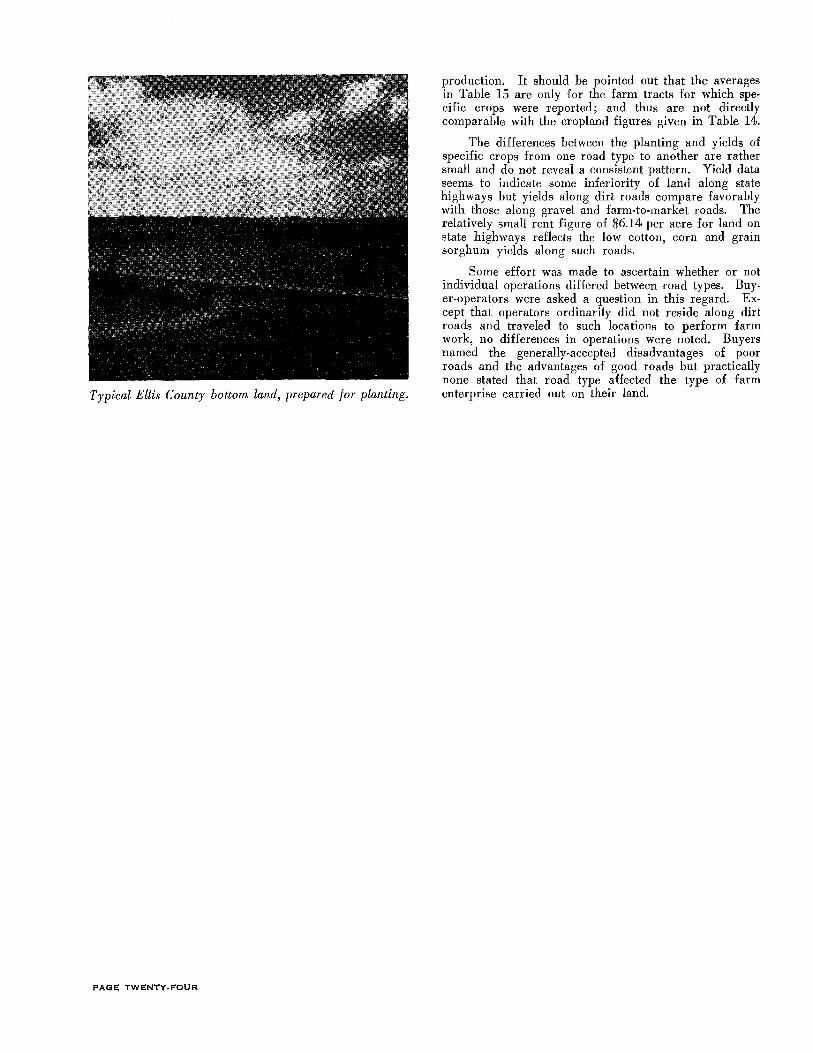
Typical Ellis County bottom land, prepared for planting.

PAGE TWENTY-FOUR

production. It should be pointed out that the averages in Table 15 are only for the farm tracts for which spe­cific crops were reported; and thus are not directly comparable with the cropland figures given in Table 14.

The differences between the planting and yields of specific crops from one road type to another are rather small and do not reveal a consistent pattern. Yield data seems to indicate some inferiority of land along state highways but yields along dirt roads compare favorably with those along gravel and farm-to-market roads. The relatively small rent figure of $6.14 per acre for land on state highways reflects the low cotton, corn and grain sorghum yields along such roads.

Some effort was made to ascertain whether or not individual operations differed between road types. Buy­er-operators were asked a question in this regard. Ex­cept that operators ordinarily did not reside along dirt roads and traveled to such locations to perform farm work, no differences in operations were noted. Buyers named the generally-accepted disadvantages of poor roads and the advantages of good roads but practically none stated that road type affected the type of farm enterprise carried out on their land.

Characteristics of Land Buyers It has been suggested in a previous section that the

particular traits of individual buyers and sellers might well have had an important influence on the exchange price of land. No attempt was made in the Ellis County study to investigate this hypothesis in detail. Because of the vast effort that would have been required, very little was determined about the sellers of land. Some information was obtained, however, on the characteristics and vehicle usage of land buyers. When inspected ac­cording to the type of road location of the land pur­chased, this information reveals several interesting pat­terns.

Buyer Characteristics and Road Type

Table 16 shows the occupation, tenure, place of resi­dence and purpose of purchase of land buyers classified by the road service of the land acquired. Buyers of land on dirt roads named farming as their main occupation less frequently than other buyers. In 1959, however, 86 percent of such buyers were operators of the tracts purchased. Owners of land on farm-to-market roads most frequently indicated that agriculture was their principal occupation, but this group had the smallest proportion of buyers who operated the land purchased. It appears that occupation had little effect on choice of type of road location, nor are the differences in tenure likely significant.

The place of residence of buyers apparently was influenced considerably by type of road service. In 1959, only 7 percent of the buyers of land on dirt roads lived on the land they had bought. Thirty percent or more of each of the other groups of buyers resided on the land purchased. Each group of buyers showed a net movement from towns and cities to farm residences by 1959. Dirt road locations obviously were not nearly so popular as those on better road types. Very few buyers had plans to move to the land they had acquired.

The most interesting finding had to do with the various purposes for buying land. Again, buyers of land on dirt roads were distinctive. About two-thirds of these buyers stated that their primary purpose for acquiring particular tracts was to add to contiguous (adjacent) holdings. Other buyer groups gave this purpose fre­quently but in far smaller proportions.

Similarly, 90 percent of the buyers who bought land on dirt roads already owned land at the time. At the opposite extreme, only 45 percent of buyers of land on farm-to-market roads had other farm land at the time of purchase. It may be concluded that land on dirt roads is prized for consolidation with other holdings but cer­tainly not for place of residence. Perhaps when owned and operated in conjunction with other land, land on dirt roads is subject to something less than the full disadvan­tages of poor road service. It is possible also that per-

Table 16

CHARACTERISTICS OF BUYERS OF LAND LOCATED ON VARIOUS ROAD TYPES, ELLIS COUNTY, 1955-58

Item

Buyer's Main Occupation in 1959: Farming Nonfarm Occupation Estate or Corporation

Buyer's Tenure in 1959: Operated on the Tract Purchased Leased-out the Tract Purchased

Buyer's Place of Residence at Time of Purchase: Tract of Land Purchased Other Farm Town or City

Buyer's Place of Residence, 1959: Tract of Land Purchased Other Farm Town or City

Buyer's Plans to Live on Tract: Lived on Tract in 1959 Plans to Move to Tract Does Not Plan to Move to Tract Uncertain No Answer

Buyer's Primary Purpose of Buying Tract: Enlarge Contiguous Farm Enlarge Noncontiguous Farm As a Home Desire to Own Land Other Investment Purpose

Buyer's Previous Farm Land Ownership: Already Owned Farm Land Did Not Own Other Farm Land

Dirt

13 (31) 27 (64) 2 ( 5)

36 (86) 6 (14)

1 ( 2) 10 (24) 31 (74)

3 ( 7) 10 (24) 29 (69)

3 ( 7) 2 ( 5) 4 (10)

31 (73) 2 ( 5)

28 (67) 6 (15) 3 ( 7) 2 ( 4) 3 ( 7)

38 (90) 4 (10)

Type of Road Location of Tract Purchased

Gravel Farm-to-Market State Highway

Number of Buyers (Percentages in Parenthesis)

35 (38) 33 (52) 7 (44) 52 (57) 29 (45) 9 (56)

5 ( 5) 2 ( 3) 0 ( 0)

82 (89) 50 (78) 14 (88) 10 (11) 14 (22) 2 (12)

2 ( 2) 4 ( 6) 1 ( 6) 36 (39) 31 (49) 5 (31) 54 (59) 29 (45) 10 (63)

28 (30) 23 (36) 5 (31) 30 (33) 25 (39) 4 (25) 34 (37) 16 (25) 7 (44)

28 (30) 23 (36) 5 (31) 1 ( 1) 1 ( 2) 1 ( 6) 6 ( 7) 8 (12) 1 ( 6)

42 (46) 26 (41) 9 (57) 15 (16) 6 ( 9) 0 ( 0)

23 (25) 11 (17) 2 (12) 15 (16) 15 (23) 3 (19) 34 (37) 25 (39) 4 (25)

6 ( 7) 4 ( 6) 1 ( 6) 14 (15) 9 (15) 6 (38)

51 (55) 35 (45) 10 (62) 41 (45) 29 (55) 6 (38)

PAGE TWENTY-FIVE

sons already owning land could foresee a greater rate of return on investments from cheaper land on dirt roads than from more expensive land on other road types. They further may have had the expectancy of better roads and were willing to wait for such improvements in view of the lower cost per acre of land.

Vehicular Trips and Annual Mileage

Buyers who either operated or resided upon the tracts which they had purchased were asked several questions regarding their travel. Owners along dirt roads admitted that rainy weather restricted their travel but stated that farm operations were generally slowed at such times anyway. In an attempt to check further on travel, buyers were requested to enumerate all trips which had been made to and from their farm tracts on the near­est past weekday and the purpose and mileage of these trips. Only trips in vehicles owned by the buyers were considered. The respondents also were asked to estimate the total mileage for each vehicle which was used to some extent in the farm business. Table 17 shows a

tabulation of the answers by type of road location of the land.

On a per-farm and per-trip basis the results are strikingly similar for each of the road types. It should be pointed out that there were no impassable roads as of the "nearest past weekdays" for which trip data were obtained. Perhaps this explains why travel was not re­stricted for land on dirt roads.

The shortest average trip length was to and from tracts on state highways. This may have occurred be­cause such tracts also were closer to both large and small towns. Locations on farm-to-market roads had the long­est trip on the average. There are other differences shown in Table 17, but most are rather minor and it is very doubtful that any are significant.

Note: Because of its bulkiness the questionnaire used in Ellis County is not included in the report. A copy may be obtained by writing to the Texas Transportation Institute, College Station, Texas.

Table 17

VEHICULAR TRIPS, TRIP PURPOSES, AND MILEAGE DATA, BY TYPE OF ROAD LOCATION 191 FARM TRAC'I'S, ELLIS COUNTY, 1959

Type of Road Location Item Dirt Gravel Farm-to-Market State Highway

Number of Tracts Operated or Occupied by Buyers 38 85 54 14

Vehicular Trips on Nearest Past Weekday: Total Trips for Household Goods 1 8 2 1 Trip Mileage for Household Goods 34 92 20 11 Total Farm Business 'I'rips 48 83 63 8 Mileage of Farm Business Trips 1050 2039 1823 220 Total Other Trips 22 61 36 15 Mileage of Other Trips 609 1541 1026 201 Total Number of All Trips 71 152 101 24 Total Mileage of All Trips 1693 3672 2869 432 Average Trips per Farm 'I'ract 1.87 1.79 1.87 1.71 Average Mileage per Farm Tract 45 43 53 31 Average Mileage per Trip 24 24 28 18

Vehicles Used in Farm Business: Number of Such Vehicles 66 156 108 25 Mileage per Vehicle, 1958 10,800 10,270 10,860 8,320 Mileage per Farm, 1958 18,700 18,850 21,720 14,860

PAGE TWENTY-SIX

Bibliography Adkins, William G., Economic Effects of the Camp Creek Road Improvement, Texas Transportation Institute, 1958.

and Southern, J. H., Texas Farm and Ranch Land Market, 1954, Report 1800, Texas Agricul­tural Experiment Station, Texas A & M, College Station.

Chambers, C. R., The Relationship of Land Income to Land Values, U.S. Dept. of Agriculture Bulletin 1224, 1923.

Ezekiel, M., Factors Affecting Farmers Earnings in Southwestern Pennsylvania, U.S. Dept. of Agriculture Bulletin 1400, 1936.

------,, Methods of Correlation Analysis, Second Edition, John Wiley & Sons, Inc. New York, 1953.

Garrison, W. L., The Benefits of Rural Roads to Rural Property, Washington State Council for Highway Re-

search, 1956.

------; Berry, Brian; Marble, Duane F.; Ny­stuen, John D.; Morrill, Richard L., Studies of Highway Development and Geographic Change, University of Washington Press, Seattle, 1959.

Haas, G. C., Sale Prices as a Basis for Farm Land Ap­praisal, Technical Bulletin 9, Agricultural Experiment Station, University of Minnesota, 1922.

Hammar, C. H., Factors Affecting Farm Land Values in Missouri, Research Bulletin 229, Agricultural Experiment Station, University of Missouri, 1935.

Harris, Karl, Factors that Give Value to Land or Basic Land Values, Bulletin 223, Agricultural Experiment Sta­tion, University of Arizona, 1949.

Highway Research Board, Developing Concepts of Land Acquisition, Bulletin 169, Washington, D.C., 1957.

------, Economic Impact of Highway Improve­ment, Special Report 28, Washington, D.C., 1957.

Ibach, D. B., "The Role of Soil Depletion in Land Valua­tion," Journal of Farm Economics, Vol. XXII, No. 2, May 1940.

Lewis, A. B., "Land Classification as an Appraisal and Credit Aid," The Classification of Land, Agricultural Ex­periment Station, University of Missouri, Bulletin 421.

Morehouse, E. W., "Land Valuation," Encyclopedia of the Social Sciences, Vol. IX, p. 137.

Murray, W. G., Farm Appraisal, Iowa State College Press, Ames, Iowa, 1950.

Parcher, L. A., The Influence of Location on Farmland Prices, Bulletin B-417, Agricultural Experiment Station, Oklahoma State University, 1954.

Stewart, C. L., "Farm Land Values as Affected by Road Type and Distance," Journal of Farm Economics, Vol. XVIII, No. 4, November, 1936.

Taylor, C. C. and Aull, G. H., Improving Farm Real Es­tate Assessment, Bulletin 450, Agricultural Experiment Station, Clemson Agricultural College, 1957.

Thompson, F. L., "Factors Affecting Real Estate Values in the United States," Journal of Farm Economics, Vol. XVII, No.2, May 1935.

U.S. Dept. of Commerce, Bureau of the Census, Census of Agriculture:1954, Volume I Part 26, Texas, 1956.

-----,Census of Agriculture: 1950, Volume I Part 26, Texas, 1952.

------1Census of Population: 1950, Volume II, Part 43, Texas, 1952.

PAGE TWENTY-SEVEN