farming systems ecology - wur · farming systems ecology: systems, landscapes and actors 1. the...

Farming Systems EcologyTowards ecological intensification of world agriculture

Prof. dr ir. Pablo A. Tittonell

Inaugural lecture upon taking up the position of Chair in Farming Systems Ecology at Wageningen University on 16 May 2013

A recurring question…

Can organic agriculture feed the world?

• Inappropriate – it deters any fruitful debate

• Misleading – complex problems require complex solutions

• Irrelevant – let’s turn it around…

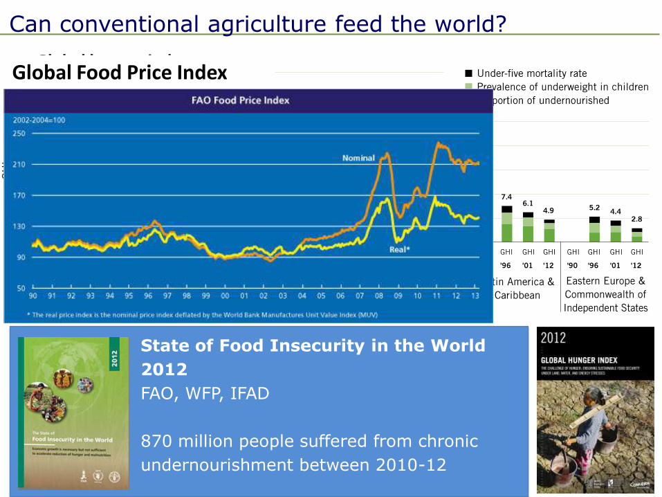
Can conventional agriculture feed the world?

TSBF, 2007

State of Food Insecurity in the World

2012

FAO, WFP, IFAD

870 million people suffered from chronic

undernourishment between 2010-12

Global hunger index


TSBF, 2007

State of Food Insecurity in the World

2012

FAO, WFP, IFAD

870 million people suffered from chronic

undernourishment between 2010-12

Global hunger indexGlobal Food Price Index


0

20

40

60

80

100

120

140

1960 1970 1980 1990 2000 2010

Monde

Chine

Brésil

France

USA

Consomation de viande per capitaMeat consumption per capita (kg/year)

TSBF, 2007


Farming Systems EcologyTowards ecological intensification of world agriculture

1. Why does current agriculture fail at feeding the world?

2. Intensify, extensify, detoxify… (ecological intensification)

3. Farming Systems Ecology: systems, actors and landscapes

Outline:


1. Worldwide, food is not produced where it is needed

2. Agricultural inputs not affordable to all farmers

3. Current diets not compatible with sustainable resource use

4. Ineffective market, storage and distribution chains

The green revolution

Production

Water & nutrients

Pesticides

Green revolution cereals:

x 2

x 7

x 3x 2

1960-2010: food calories produced increased by 179% while population grew by 117%


Production

Water & nutrients

Pesticies


50 Pg of carbon lost from the world soils

x 2

x 7

x 3x 2

0

1

2

3

4

5

6

7

8

1960 1970 1980 1990 2000 2010

France

United States

China

Brazil

Kenya

Burkina Faso

Cereal productivity (t ha-1

year-1

)Cereal productivity (t ha-1 yr-1)

0

50

100

150

200

250

300

350

1960 1970 1980 1990 2000 2010

Fertiliser use intensity (t ha-1

year-1

)Fertiliser use intensity (kg ha-1 yr-1)

1960-2010: food calories produced increased by 179% while population grew by 117%Fertiliser N use efficiency in China (Ju et al., 2009)

Year

Grain Production

(M tonnes)

N fertiliser

(M tonnes)

PFPN

(kg/kg)

1977 283 7.07 40.0

2005 484 26.21 18.5

% change 71% 271% -54%


Production

Water & nutrients

Pesticies


50 Pg of carbon lost from the world soils

x 2

x 7

x 3x 2

0

1

2

3

4

5

6

7

8

1960 1970 1980 1990 2000 2010

France

United States

China

Brazil

Kenya

Burkina Faso

Cereal productivity (t ha-1

year-1

)Cereal productivity (t ha-1 yr-1)

0

50

100

150

200

250

300

350

1960 1970 1980 1990 2000 2010

Fertiliser use intensity (t ha-1

year-1

)Fertiliser use intensity (kg ha-1 yr-1)

1960-2010: food calories produced increased by 179% while population grew by 117%Fertiliser N use efficiency in China (Ju et al., 2009)

Year

Grain Production

(M tonnes)

N fertiliser

(M tonnes)

PFPN

(kg/kg)

1977 283 7.07 40.0

2005 484 26.21 18.5

% change 71% 271% -54%

With the excess fertiliser used by Chinese farmers it is possible to fertilise the whole of SS Africa at a rate of 60 kg/ha (Ju et al., 2009)

Obesity outweighs hunger

Food demand increases as incomes rise



Prevalence of undernourishment

1300 million obese people worldwide(WHO, 2012)



Prevalence of undernourishmentPrevalence of obesity




Prevalence of undernourishmentPrevalence of obesity


65% of the world population lives in countries where obesity kills more people than hunger (WHO, 2012)

Waste causes hunger

In India, 21 million tonnes of wheat is wasted each year due to inadequate

storage and distribution systems (FAO, 2011)

Waste causes hunger

In India, 21 million tonnes of wheat is wasted each year due to inadequate

storage and distribution systems (FAO, 2011)

It is estimated that 30 to 50% of all food produced (or 1.2 to 2 billion tonnes) never reaches the human stomach (Gustavsson et al., 2011; FAO)

1. Worldwide, food is not produced where it is most needed

2. Agricultural inputs not affordable to all farmers

3. Current diets not compatible with sustainable resource use

4. Ineffective market, storage and distribution chains

Ecological intensification

2. Intensify in the South, extensify in the North, detoxify everywhere…

Change is much needed…

Resources/ investment

Att

ain

able

pro

du

ctiv

ity

Poverty traps

Inefficiency and pollution

Eco-efficiency possible

Context

Co

nte

xt

Intensify, extensify, detoxify…

Resources/ investment

Att

ain

able

pro

du

ctiv

ity

Poverty traps

Inefficiency and pollution

‘Intensification ‘Ecologisation’

Eco-efficiency possible

Context

Co

nte

xt

Intensify, extensify, detoxify…

‘Ecologisation’: How to maintain productivity while reducing fossil fuel inputs?

‘Intensification’: How to increase productivity in a sustainable, affordable way?

Organic vs. conventional yields


Seufert et al., 2012

Organic vs. Conventional crop yields




Org.%Yield%%=%0.81%*%Conv.%Yield%4%0.15%R²%=%0.81%

0"

2"

4"

6"

8"

10"

12"

14"

16"

0" 2" 4" 6" 8" 10" 12" 14" 16"

0,0"

0,2"

0,4"

0,6"

0,8"

1,0"

1,2"

1,4"

1,6"

1,2

"

1,6

"

1,9

"

2,2

"

2,4

"

2,4

"

2,7

"

3,1

"

3,3

"

3,4

"

3,7

"

3,8

"

4,2

"

4,4

"

4,5

"

4,6

"

4,9

"

5,0

"

5,1

"

5,3

"

5,4

"

5,5

"

5,8

"

5,9

"

6,1

"

6,2

"

6,4

"

6,6

"

6,6

"

6,9

"

7,3

"

8,2

"

8,8

"

10

,1"

11

,8"

12

,3"

0"

2"

4"

6"

8"

10"

12"

0"to"3.3" 3.3"to"5.0" 5.0"to"6.4" 6.4"to"13.7"

Organic"

Conven: onal"

Org

anic

yie

ld (

t h

a-1

)

Conventional yield (t ha-1)

Avera

ge y

ield

(t h

a-1

)

1:1 lin

e

0.84 0.77 0.75 0.79

Organic vs. conventional cereal yieldsDe Ponti et al., 2012




Org.%Yield%%=%0.81%*%Conv.%Yield%4%0.15%R²%=%0.81%

0"

2"

4"

6"

8"

10"

12"

14"

16"

0" 2" 4" 6" 8" 10" 12" 14" 16"

0,0"

0,2"

0,4"

0,6"

0,8"

1,0"

1,2"

1,4"

1,6"

1,2

"

1,6

"

1,9

"

2,2

"

2,4

"

2,4

"

2,7

"

3,1

"

3,3

"

3,4

"

3,7

"

3,8

"

4,2

"

4,4

"

4,5

"

4,6

"

4,9

"

5,0

"

5,1

"

5,3

"

5,4

"

5,5

"

5,8

"

5,9

"

6,1

"

6,2

"

6,4

"

6,6

"

6,6

"

6,9

"

7,3

"

8,2

"

8,8

"

10

,1"

11

,8"

12

,3"

0"

2"

4"

6"

8"

10"

12"

0"to"3.3" 3.3"to"5.0" 5.0"to"6.4" 6.4"to"13.7"

Organic"

Conven: onal"

Org

anic

yie

ld (

t h

a-1

)

Conventional yield (t ha-1)

Avera

ge y

ield

(t h

a-1

)

1:1 lin

e

0.84 0.77 0.75 0.79

Organic vs. conventional cereal yieldsDe Ponti et al., 2012

Research investment gap between organic and conventional agriculture?e.g.,

Dutch government = 4 million euro/yearMonsanto = 980 million dollars/year (www.monsanto.com/investors)

Biological N2 fixation

Maize-Pigeon pea intercrops in Southern Africa

No interference Relaying effect Nutrient cycling




Mai

ze g

rain

yie

ld (

t h

a-1)

Residual effects on maize

Ruzinamhodzi et al., 2012




Mai

ze g

rain

yie

ld (

t h

a-1)

Residual effects on maize

Ruzinamhodzi et al., 2012

More than fivefold yield increase without fertilisers!

Net primary productivity = 1 to 2 t/ha/year Net primary productivity = 10 to 20 t/ha/year

Agricultural field (millet/cowpea) Savannah vegetation (under use)

Designing agricultural systems by mimicking nature

Simplistic approaches will not work…

3. Farming systems ecology: systems, landscapes and actors

Simplistic approaches will not work…

3. Farming systems ecology: systems, landscapes and actors

1. The yield gap between organic and conventional agriculture is to large extent a research investment gap

2. Great potential to intensify symbiotic N fixation; yet nutrient management is a bottleneck for up-scaling ecological farming

3. Green revolution technologies do not work on degraded or fragile soils: need to draw inspiration from nature

4. We need systems approaches that embrace landscape-level processes and the communities that manage and/or live on them

Input Output

Input Output

Specialized System

Agro-diverse System

Externalities

Externalities

Produce more, but produce differently…

Ecoefficie

ncie

s

Input Output

Specialized System

Externalities

Input Output

Input Output

Specialized System

Agro-diverse System

Externalities

Externalities

Produce more, but produce differently…

Ecoefficie

ncie

s

Input Output

Specialized System

Externalities

Pursuing narrowly-defined efficiency reduces systems resilience (Walker et al., 2009)

Design

Analysis

Synthesis

Structure

Function

Purpose

Purpose

Function

Structure

New facts, new realities

Conclusions Decisions

Knowledge

Questions

Problems

Reality (current agroecosystems)

Adapted from: Goewie, 1993

Ecological intensification requires systems re-design

Rice-ducks-fish-azolla - Indonesia

Khumairoh et al., 2012

Building upon local agroecological knowledge

Rice-ducks-fish-azolla - Indonesia

Khumairoh et al., 2012

Building upon local agroecological knowledge

Rice yield (t ha-1) at increasing levels of complexity

0

2

4

6

8

10

12

Rice Rice+ducks

Rice+compost

Rice+ducks+

fish

Rice+compost+azolla

Rice+ducks+

compost

Rice+ducks+fish+

compost

Rice+ducks+

compost+azolla

Rice+ducks+fish+

compost+azolla

Guiera senegalensis

Piliostigma reticulatum

Facilitation of crop production

through association with native woody

species (Lahmar et al., 2012)

Native resources and local knowledge in the Sahel

Guiera senegalensis

Piliostigma reticulatum

Facilitation of crop production

through association with native woody

species (Lahmar et al., 2012)

Native resources and local knowledge in the Sahel

Understanding traditional soil fertility management

Understanding/optimising local practices

Thesis: Georges Félix, FSE

Understanding/optimising local practices

Allée1-1.4

Evac

uatio

n de

s eau

x de

ruis

selle

men

t

Rue

du C

IRAD

Z-N

SZ-

MSD

Z-LS

DN

T-LS

DN

T-HS

D

Z-HS

D

NT-

LSD

Z-N

SZ-

MSD

Z-HS

D

NT-

HSD

Rue du Burkina Faso

Avenue de l'Afrique

Rue du Zimbabwe

Rue du Kenya

Rue de Madagascar

Z-N

SN

T-LS

DZ-

LSD

Z-HS

DN

T-LS

DZ-

NS

Z-M

SDZ-

LSD

NT-

HSD

Réserve de Piliostigma reticulatum

Rue

de la

Fon

datio

n 2i

E

NT-

HSD

Z-HS

DZ-

MSD

NO

RD

Boul

evar

d de

l'U

nion

Eur

opée

nne

Z-LS

D

NS-No shrub LSD-Low Shrub Density, Spacing (6,4 x 3,2) m

(17x25 = 425 planting pits or zai holes) 414 planting pits or zai holes and 11 shrubs

MSD-Medium Shrub Density, Spacing (3,2 x 3,2)m HSD-High Shrub Density, Spacing (1,6 x 3,2)m

407 planting pits and 18 shrubs 393 planting pits and 32 shrubs

Thesis: Georges Félix, FSE

Cortez-Arriola et al. (2013)

Sustainable intensification pathways

Ecological services Ecological services

Farm productivity gap



Productivity per animal








Productivity per unit labour







0

400

800

1200

1600

2000

2400

-20 0 20 40 60 80

Lab

or

bal

ance

(h)

a.

-500

-250

0

250

500

-20 0 20 40 60 80Org

anic

mat

ter

bal

ance

(kg/

ha)

b.

-500

-250

0

250

500

0 400 800 1200 1600 2000 2400

c.

0

10

20

30

40

50

60

70

80

-20 0 20 40 60 80

Operating profit (k€)

So

il n

itro

gen

lo

ss (

kg/

ha) d.

0

10

20

30

40

50

60

70

80

0 400 800 1200 1600 2000 2400

Labor balance (h)

e.

0

10

20

30

40

50

60

70

80

-500 -250 0 250 500

Organic matter balance (kg/ha)

f.

Groot et al., 2012. Agricultural Systems.

Trade-offs at farm scale

Labour (h)Profit (K$) SOM (kg/ha)

SOM

(kg

/ha)

Lab

ou

r (h

)N

loss

es (

kg/h

a)







0

400

800

1200

1600

2000

2400

-20 0 20 40 60 80

Lab

or

bal

ance

(h)

a.

-500

-250

0

250

500

-20 0 20 40 60 80Org

anic

mat

ter

bal

ance

(kg/

ha)

b.

-500

-250

0

250

500

0 400 800 1200 1600 2000 2400

c.

0

10

20

30

40

50

60

70

80

-20 0 20 40 60 80

Operating profit (k€)

So

il n

itro

gen

lo

ss (

kg/

ha) d.

0

10

20

30

40

50

60

70

80

0 400 800 1200 1600 2000 2400

Labor balance (h)

e.

0

10

20

30

40

50

60

70

80

-500 -250 0 250 500

Organic matter balance (kg/ha)

f.

Groot et al., 2012. Agricultural Systems.

Trade-offs at farm scale

Labour (h)Profit (K$) SOM (kg/ha)

SOM

(kg

/ha)

Lab

ou

r (h

)N

loss

es (

kg/h

a)Exploring strategies to narrow the farm productivity gap

EnvironmentProfitabilityCompromise

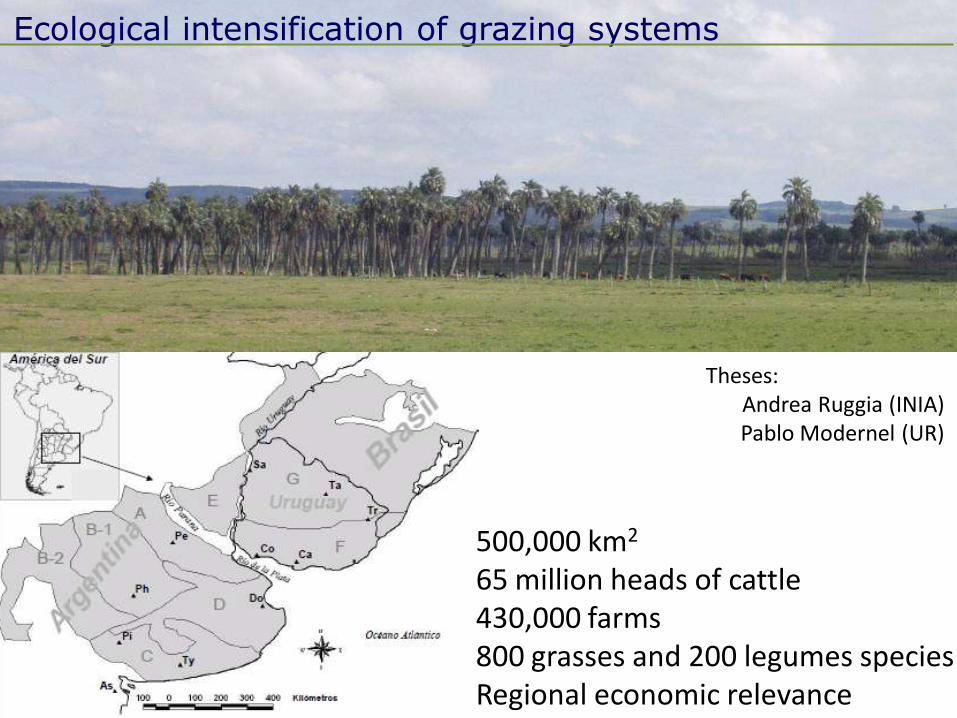
Ecological intensification of grazing systems

Theses:Andrea Ruggia (INIA)Pablo Modernel (UR)

500,000 km2

65 million heads of cattle430,000 farms800 grasses and 200 legumes speciesRegional economic relevance

Ecological intensification of grazing systems

Theses:Andrea Ruggia (INIA)Pablo Modernel (UR)

500,000 km2

65 million heads of cattle430,000 farms800 grasses and 200 legumes speciesRegional economic relevance

GHG emissions

Energy consumption

Soil erosion N surplus P surplus Pesticide contamination

Environmental impact of different intensification pathways

Traditional system

Feedlot

Modernel et al., sbmtd.

Designing pest suppressive landscapes

Hawassa, Ethiopia

Thesis: Yodit Kabede


55

La Figure 19 montre l’index d’infestation moyen des champs selon la zone écologique

dans lesquels ils se trouvent. La sous-zone 3 montre une tendance à être plus infestée par les

pucerons, bien que l’analyse de la déviance ne montre pas d’effet des sous-zones écologiques

sur le niveau d’infestation.

Pour visualiser les différences spatialisées dans la dynamique d’infestation, les

données sont comparées selon les sous-zones écologiques dans la Figure 20.

Figure 20. I ndex d’ infestation moyen des champs en fonction des semaines de relevés, pour les quatre zones écologiques. K ajulu, K enya, 2011

Sur la base de ces données, des dynamiques d’infestation différentes se dessinent selon

les sous-zones écologiques. La sous-zone écologique 3 présente en effet un index

d’infestation supérieur à celui des autres sous-zones, en début de période : jusqu’à la

3esemaine. Or cette sous-zone écologique est caractérisée par un intense réseau de haies, et

une mosaïque de champs très fine. Si la concentration en plantes hôtes des pucerons Aphis craccivora et Aphis fabae joue le rôle de refuge pour les pucerons, ceci pourrait expliquer une

infestation plus importante dans les champs, dès le début du cycle de culture du haricot.

Concernant l’infestation en sous-zone écologique 4, elle commence à un niveau plus

faible mais sa pente est plus forte. Or cette zone-ci se caractérise par l’absence de haies, et un

paysage plus ouvert que les autres zones. La sous-zone écologique 3 pourrait donc jouer le

rôle de réservoir à pucerons pour les autres sous-zones alentours.

Les index d’infestation dessous-zones écologiques 1 et 2 sont représentés dans ce

graphique à partir d’un seul jeu de données : un seul champ était suivi pour chacune de ces

sous-zones (sauf en semaine 5, où les données sont issues de l’observation ponctuelle des

champs). Ces résultats sont donc difficiles à interpréter.

En semaine 5, le niveau d’infestation des champs suivis ponctuellement est alors

équivalent dans toutes les sous-zones écologiques représentées.

0

0,5

1

1,5

2

2,5

3

3,5

4

4,5

S1 S2 S3 S4 S5

Index d'infestation moyen

ZE 1

ZE 2

ZE 3

ZE 4

Spatio-temporal variation

Infestation index

Week 1 Week 2 Week 3 Week 4 Week 5

Zones

Hawassa, Ethiopia



55
























0

0,5

1

1,5

2

2,5

3

3,5

4

4,5

S1 S2 S3 S4 S5


ZE 1

ZE 2

ZE 3

ZE 4


Infestation index


Zones

Study area

Hawassa, Ethiopia



55
























0

0,5

1

1,5

2

2,5

3

3,5

4

4,5

S1 S2 S3 S4 S5


ZE 1

ZE 2

ZE 3

ZE 4


Infestation index


Zones

Study area

Hawassa, Ethiopia

Bio

co

ntr

ol

Pesticide needCurrent

landscapeGroot and Rossing, 2010

Exploration of alternative landscape structures


Collective decision making on natural resources

Simulation and gaming for improving local adaptive capacity;The case of a buffer-zone community in Mexico

E.N. Speelman

Mapa de la Reserva de la Biosfera de la Sepultura. Fuente: CONANP

Actors

LandscapesSystems

Agroecology

Farming Systems Ecology

Farming Systems Ecology (FSE) research strategy

Farming systems ecology

Crop & weed ecology

Soil quality group

Organic plant breeding

Animal production systems

Plant production systems

Farm technology group

Innovation & communication

studies

Rural sociology

• Ecological intensification

• Systems design as core business

• Interface between ecology and society

• Parallel strategies for the North (Europe) and the South (Tropics)

Guiding principles

Collaboration

Discipline

FSE in the world (PhD theses)

On-going

Inherited (France)

Starting 2012/3

Actors

LandscapesSystems

Agroecology

FarmingSystemsEcology

A conventional farmer purchasing pesticides

An agroecological farmer inspecting his intercrop

Communication and image

Photo: Steve Sherwood Photo: Clarin Rural

A conventional farmer purchasing pesticides

An agroecological farmer inspecting his intercrop

Communication and image

Photo: Steve Sherwood Photo: Clarin Rural

Estancia Laguna Blanca, Entre Rios, ArgentinaEcological farming on 3000 ha

Ecologically intensive farming is more than just

conventional farming without inputs

It requires:

- ecological engineering at farm and landscape level

- ability to engage with local actors and learn from them

- systems approaches that embrace the complexity of social-ecological

interactions

It needs:

- Serious public funding that compensates for the investment gaps

Intensify in the South, extensify in the North,

detoxify everywhere…

Concluding remarks

farming systems ecology - wur · farming systems ecology: systems, landscapes and actors 1. the...

Documents