fast footstep planning with aborting a*
TRANSCRIPT

Fast Footstep Planning with Aborting A*
Marcell Missura and Maren Bennewitz
Abstract— Footstep planning is the dominating approachwhen it comes to controlling the walk of a humanoid robot,even though a footstep plan is expensive to compute. The mostprominent proposals typically spend up to a few seconds ofcomputation time and output a sequence of up to 30 steps all theway to the goal. This way, footstep planning is applicable only instatic environments where nothing changes after a plan has beencomputed. Since uncontrolled environments present challengessuch as unforeseen motion of other objects and unexpecteddisturbances to balance, fast replanning of a footstep plan whilethe robot is in motion is highly desirable. We present a newway of fast footstep planning - Aborting A* - which is able toguarantee a replanning rate of 50 Hz by aborting an A* searchbefore completion. We make aborting possible by using a novel,obstacle-aware heuristic function that lays out rotate-translate-rotate motions along the shortest path to the goal, enabling us tostop the planning progress prematurely with a target-orientedsolution at any time during the search, even after only a fewnodes have been expanded. We show in our experiments thatdespite the bounded computation time, our planner computesgood results and does not get stuck in local minima.
I. INTRODUCTION
The discrete footsteps of a humanoid robot naturally lendthemselves for navigation and control when a footstep planis computed in order to determine where the robot shouldplace its next steps. Most research revolving around this topichas converged to regarding footstep planning as a graph-search and using the A* algorithm to solve it. Respectableresults have been achieved that manage to walk humanoidrobots over slanted cinder blocks and narrow beams and tostep over obstacles [1]. So far, the prominent approach isto compute a long sequence of footsteps that reach all theway to the target and to follow the footsteps as closely aspossible using precise motion tracking. These plans oftenconsist of 30 steps or more, requiring up to a few secondsof computation time to produce. At this time scale, it is notpractical to replan while the robot is in motion. Realisticenvironments, however, constantly present unforeseen eventsthat necessitate replanning. Moving obstacles can changedirection in unpredictable ways and require fast reaction toavoid a collision. Disturbances to balance need to be dealtwith quickly to avoid falling. Drifting away from the planduring execution is also best solved by replanning. It ishighly desirable to meet these challenges with a controllerthat has a short and guaranteed response time.
At the same time, finishing a plan all the way to thegoal is indeed necessary in order to keep the system fromgetting stuck forever in local traps. The computation of aplan to completion and a controller response in bounded-time
All authors are with the Humanoid Robots Lab, University of Bonn,Germany. Contact: [email protected]
Fig. 1: Example footstep plan with cluttered objects on the floor.20 footsteps were computed towards the intermediate target withina computation time limit of 20 milliseconds. The cyan circle marksthe start state, the yellow circle marks the goal state. The smallerorange circle is an intermediate target at the boundary of the localmap outside of which only a 2D path is planned (thick blue line).The areas shaded in red indicate regions where the feet must not beplaced and the green colored region show polygons that are usedfor shortest path planning.
appear to be, however, mutually exclusive. Consequently,our navigation system is made of two components runningat different time scales. One is a global path planner thatplans all the way to the goal and has the time to do sobecause the second, a fast-paced but short-sighted footstepcontroller, takes the responsibility for control actions thathave to happen quickly. The global planner informs thefootstep controller of an intermediate target that the robot isto aim for in order to progress towards the global goal andit is up to the footstep controller to figure out the next stepsto take towards this intermediate goal while negotiating thechallenges of the environment with a high response rate. Nowwith our contribution, A* footstep planning can be used torealize a high-frequency footstep controller with a guaranteedresponse time of 20 milliseconds. The key concepts toachieve such low computation times are a bounded area forplanning and a novel heuristic that lays out rotate-translate-rotate motions along the shortest path to the goal and allowsaborting the search prematurely before the target was found.
II. RELATED WORK
The origins of A* footstep planning lie in the pioneeringwork of Kuffner et al. [2], [3] and Chestnut et al. [4] whorealized an online footstep planner for the ASIMO robot thatcould run at a rate of roughly 1 Hz. A binary occupancymap served as environment representation and a simple A*search was used with only two cost components for stepcosts and environment costs. The heuristic was precomputedusing a wheeled robot model. Even though the heuristic

was not admissible, it helped to guide the search aroundnon-traversable obstacles towards the target and the footstepplanner computed good solution paths in reasonable time.
Ayaz et al. [5] presented another early approach to stepover obstacles with the HRP-2 robot. The possible footsteplocations were strongly constrained and several simplifyingassumptions were made. As a result, the set of planningproblems that could be solved was limited and the resultingplans were not optimal.
Hornung et al. [6] [7] investigated different flavours ofthe A* algorithm [8] for footstep planning in a planar envi-ronment. The authors implemented a footstep planner usingR* and ARA* with the Euclidean and the Dijkstra heuristic.Anytime Repairing A* (ARA*) [9] computes multiple passeswith an inflated heuristic where the inflation factor decreaseswith each run. This way, a suboptimal solution can be foundquicker than with A* and the quality of the solution increaseswith time. R* [10] is a probabilistic version of A* thatsamples the state space and concentrates on the states thatcan be reached quickly. Both A* variates come with a boundon the suboptimality of the solution. Hornung et al. alsoproposed a mixed level-of-detail solution [11] where in freespace only a 2D path is computed and single footsteps areplanned only in the close vicinity of obstacles. With thisapproach, the authors achieved a planning rate of 2 to 3 Hz.Garimort et al. [12] proposed to use D*-Lite [13] for footstepplanning due to its replanning capabilities. The authorsshowed that after an initial computation around the 1 secondmark, the footstep plan can be updated during walking at arate of approximately 2 Hz.
With the wind of the Darpa Humanoid Challenge in 2015,numerous instances of footstep planners have been presented[1] [14] [15] [16] [17] [18] that surpassed the earlier planarwalkers with 3D walking capabilities. Driven by the tasksof the competition, human operator-guided systems emergedcomplete with point-cloud processing and features such asoverstepping gaps and walking on surfaces made of slantedcinder blocks. Since the environment was static during thecompetition, fast replanning capabilities were not needed.The work of Griffin et al. [1] is a most refined versionof such a footstep planner where based on a geometricworld representation, the planning functionalities have beenextended with more precise treatment of edges leading up toa humanoid robot being able to walk along a narrow beamno wider than the foot of the robot. Deits et al. [19] [14]presented an alternative approach to A* footstep planning us-ing a mixed-integer quadratic program optimization. It relieson a segmentation of the environment into convex regions.The computation time needed for all of the aforementionedapproaches ranges up to a few seconds.
Hildebrandt et al. [20] [21] proposed the most completeapproach to footstep planning to our knowledge. The authors’framework includes a 3D perception module [22] wherewalkable surfaces are modeled as planes and all other objectsas swept sphere volumes, which support real-time collisionchecking [23]. The included A* planner can overstep obsta-cles and is supported by a reactive balance controller. The
system can walk in an unsupervised manner driven only byonboard sensing and replans during walking at a pace ofaround 5 Hz. So far, the system has been tested only in flatand open environments with small, convex objects. Sincethe Euclidean heuristic is used for the A* search, protrudingobstacles can drastically impair performance.
Perrin et al. [24] used swept volume approximations forefficient 3D collision checking up to a certain height andperform 2D footstep planning. While this approach findscollision-free footstep plans in cluttered environments, itdoes not possess real-time capabilities. Karkowski et al. [25]considered the use of a limited horizon in order to acceleratethe planning speed. The step action set was adapted to theterrain on the fly respecting reachability constraints. Thisapproach has achieved remarkable runtimes around the 50millisecond mark in small and simple environments wherethe target was placed in front of the robot and no obstaclesblock the way. Since the planner uses a forward-directedheuristic, it is likely to degrade in obstacle-rich situations.
Our contribution over the aforementioned works is theinclusion of the shortest path into the heuristic functionand the formulation of the Path RTR (rotate-translate-rotate)function that greatly helps to guide the search along theshortest path and achieves true abortability. To the best ofour knowledge, we are the first to breach a replanning rateof 50 Hz.
III. ABORTING A*
A. Prerequisites for Footstep Planning
We envision our footstep planner to be a part of a largerrobot operating system where a global map and localizationin the map already exist. We assume to be given a startpose S = (xS , yS , θS) and a goal pose G = (xG, yG, θG) inthe global reference frame where x and y are the Cartesiancoordinates of a pose and θ is the orientation. We also assumeto be given a global 2D path P (S,G) = {(xi, yi) | i = 0..k}where (x0, y0) = (xS , yS) and (xk, yk) = (xG, yG).
B. Planning in a Local Map
We confine the operational area of our footstep planner toa local map as shown in Figure 1. The local map is a squareof 8m× 8m that extends four meters to the left and right,six meters to the front, and two meters to the back of therobot. Footstep planning and shortest path computations takeplace only within the local map. Outside of the local map,the global path P completes the plan.
The global path from S to G is intersected with the localmap in order to determine an intermediate goal pose G thatserves as a target for the planning within the local map. Theintersection is computed such that the global path is followedfrom the start towards the goal until the first intersectionwith the boundary of the local map is found, or the goal isreached. Thus, the intermediate goal G is located either onthe boundary of the local map, or inside the local map if theentire path lies inside in which case G = G. The start andgoal poses and the intermediate goal are illustrated in Fig. 1.
dilate
input grid
collision grid
path search map
path search grid
erode + dilate dilate polygonize
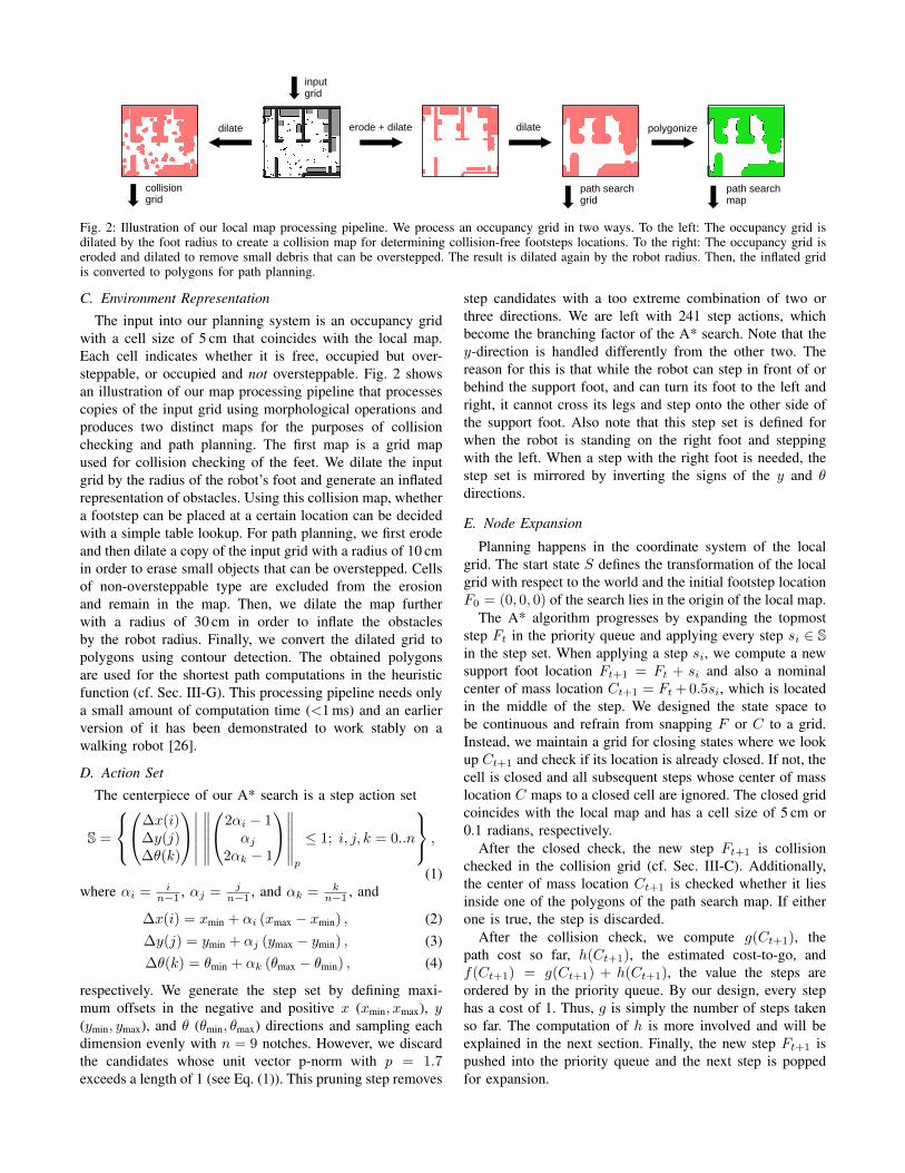
Fig. 2: Illustration of our local map processing pipeline. We process an occupancy grid in two ways. To the left: The occupancy grid isdilated by the foot radius to create a collision map for determining collision-free footsteps locations. To the right: The occupancy grid iseroded and dilated to remove small debris that can be overstepped. The result is dilated again by the robot radius. Then, the inflated gridis converted to polygons for path planning.
C. Environment Representation
The input into our planning system is an occupancy gridwith a cell size of 5 cm that coincides with the local map.Each cell indicates whether it is free, occupied but over-steppable, or occupied and not oversteppable. Fig. 2 showsan illustration of our map processing pipeline that processescopies of the input grid using morphological operations andproduces two distinct maps for the purposes of collisionchecking and path planning. The first map is a grid mapused for collision checking of the feet. We dilate the inputgrid by the radius of the robot’s foot and generate an inflatedrepresentation of obstacles. Using this collision map, whethera footstep can be placed at a certain location can be decidedwith a simple table lookup. For path planning, we first erodeand then dilate a copy of the input grid with a radius of 10 cmin order to erase small objects that can be overstepped. Cellsof non-oversteppable type are excluded from the erosionand remain in the map. Then, we dilate the map furtherwith a radius of 30 cm in order to inflate the obstaclesby the robot radius. Finally, we convert the dilated grid topolygons using contour detection. The obtained polygonsare used for the shortest path computations in the heuristicfunction (cf. Sec. III-G). This processing pipeline needs onlya small amount of computation time (<1 ms) and an earlierversion of it has been demonstrated to work stably on awalking robot [26].
D. Action Set
The centerpiece of our A* search is a step action set
S =
∆x(i)
∆y(j)∆θ(k)
∣∣∣∣∣∣∥∥∥∥∥∥2αi − 1
αj2αk − 1
∥∥∥∥∥∥p
≤ 1; i, j, k = 0..n
,
(1)where αi = i
n−1 , αj = jn−1 , and αk = k
n−1 , and
∆x(i) = xmin + αi (xmax − xmin) , (2)∆y(j) = ymin + αj (ymax − ymin) , (3)∆θ(k) = θmin + αk (θmax − θmin) , (4)
respectively. We generate the step set by defining maxi-mum offsets in the negative and positive x (xmin, xmax), y(ymin, ymax), and θ (θmin, θmax) directions and sampling eachdimension evenly with n = 9 notches. However, we discardthe candidates whose unit vector p-norm with p = 1.7exceeds a length of 1 (see Eq. (1)). This pruning step removes
step candidates with a too extreme combination of two orthree directions. We are left with 241 step actions, whichbecome the branching factor of the A* search. Note that they-direction is handled differently from the other two. Thereason for this is that while the robot can step in front of orbehind the support foot, and can turn its foot to the left andright, it cannot cross its legs and step onto the other side ofthe support foot. Also note that this step set is defined forwhen the robot is standing on the right foot and steppingwith the left. When a step with the right foot is needed, thestep set is mirrored by inverting the signs of the y and θdirections.
E. Node Expansion
Planning happens in the coordinate system of the localgrid. The start state S defines the transformation of the localgrid with respect to the world and the initial footstep locationF0 = (0, 0, 0) of the search lies in the origin of the local map.
The A* algorithm progresses by expanding the topmoststep Ft in the priority queue and applying every step si ∈ Sin the step set. When applying a step si, we compute a newsupport foot location Ft+1 = Ft + si and also a nominalcenter of mass location Ct+1 = Ft + 0.5si, which is locatedin the middle of the step. We designed the state space tobe continuous and refrain from snapping F or C to a grid.Instead, we maintain a grid for closing states where we lookup Ct+1 and check if its location is already closed. If not, thecell is closed and all subsequent steps whose center of masslocation C maps to a closed cell are ignored. The closed gridcoincides with the local map and has a cell size of 5 cm or0.1 radians, respectively.
After the closed check, the new step Ft+1 is collisionchecked in the collision grid (cf. Sec. III-C). Additionally,the center of mass location Ct+1 is checked whether it liesinside one of the polygons of the path search map. If eitherone is true, the step is discarded.
After the collision check, we compute g(Ct+1), thepath cost so far, h(Ct+1), the estimated cost-to-go, andf(Ct+1) = g(Ct+1) + h(Ct+1), the value the steps areordered by in the priority queue. By our design, every stephas a cost of 1. Thus, g is simply the number of steps takenso far. The computation of h is more involved and will beexplained in the next section. Finally, the new step Ft+1 ispushed into the priority queue and the next step is poppedfor expansion.
In accordance with our Aborting A*, we check after everypop whether either a limit on the number of expansionshas been reached, or the computation time has run out. Ifeither of the abort conditions is met, we return the step withthe smallest h value found so far. We chose the state withthe lowest heuristic, because the last opened step can beanywhere in the graph, but the step with the lowest h value issure to reach closest to the target. If a popped step reaches aheuristic value h(Ct) < 0.5 (less than half a step), the searchis halted and the last opened step is returned as a solutionfrom which parent pointers are followed to reconstruct thestep sequence.
F. Heuristic Function
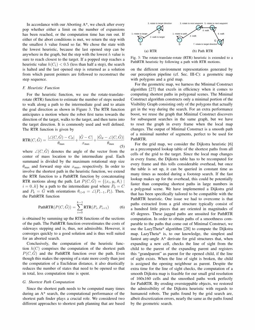
For the heuristic function, we use the rotate-translate-rotate (RTR) function to estimate the number of steps neededto walk along a path to the intermediate goal and to attainthe goal direction as shown in Figure 3. The RTR functionanticipates a motion where the robot first turns towards thedirection of the target, walks to the target, and then turns intothe target direction. It is commonly used and well defined.The RTR function is given by
RTR(C, G) =|∠(C, G)− Cθ|
θmax+|G− C|xmax
+|Gθ − ∠(C, G)|
θmax(5)
where ∠(C, G) denotes the angle of the vector from thecenter of mass location to the intermediate goal. Eachsummand is divided by the maximum rotational step sizeθmax and forward step size xmax, respectively. In order toinvolve the shortest path in the heuristic function, we extendthe RTR function to a PathRTR function by concatenatingRTR motions along the path. Let P (C, G) = {(xi, yi, θi) |i = 0..k} be a path to the intermediate goal where P0 = Cand Pk = G with orientations θi>0 = ∠(Pi−1, Pi). Then,the PathRTR function
PathRTR(P (C, G)) =
k−1∑i=0
RTR(Pi, Pi+1) (6)
is obtained by summing up the RTR functions of the sectionsof the path. The PathRTR function overestimates the costs ofsideways stepping and is, thus, not admissible. However, itconverges quickly to a good solution and is thus well suitedfor an aborted search.
Conclusively, the computation of the heuristic func-tion h(C) comprises the computation of the shortest pathP (C, G) and the PathRTR function over the path. Eventhough this makes the opening of a state more costly than justthe computation of a Euclidean distance, it also drasticallyreduces the number of states that need to be opened so thatin total, less computation time is spent.
G. Shortest Path Computation
Since the shortest path needs to be computed many timesduring an A* search, the computational performance of theshortest path finder plays a crucial role. We considered twodifferent approaches to shortest path planning that are based
1. rotate to target
2. walk to target
3. rotate to target direction
S
G
(a) RTR
1. rotate to path2. walk
3. rotate to next waypoint
S
G
4. walk
5. rotate to next waypoint
6. walk
7. rotate to target direction
(b) Path RTR
Fig. 3: The rotate-translate-rotate (RTR) heuristic is extended to aPathRTR heuristic by following a path with RTR motions.
on the different environment representations generated byour perception pipeline (cf. Sec. III-C): a geometric mapwith polygons and a grid map.
For the geometric map, we harness the Minimal Constructalgorithm [27] that excels in efficiency when it comes tocomputing shortest paths in polygonal scenes. The MinimalConstruct algorithm constructs only a minimal portion of theVisibility Graph consisting only of the polygons that actuallyget in the way during the search. For an extra performanceboost, we reuse the graph that Minimal Construct discoversfor subsequent searches in the same graph, but we haveto reset the graph in every frame when the local mapchanges. The output of Minimal Construct is a smooth pathof a minimal number of segments, perfect to be used forPathRTR.
For the grid map, we consider the Dijkstra heuristic [6]as a precomputed lookup table of the shortest paths from allcells of the grid to the target. Since the local map changesin every frame, the Dijkstra table has to be recomputed forevery frame and this tolls considerable overhead, but oncethe table is set up, it can be queried in constant time asmany times as needed during a footstep search. If the fastlookup makes up for the overhead, this could be potentiallyfaster than computing shortest paths in large numbers ina polygonal scene. We have implemented a Dijkstra gridthat has been specifically tailored to be compatible with thePathRTR heuristic. One issue we had to overcome is thatpaths extracted from a grid structure typically consist ofa hundred little pieces that are oriented in magnitudes of45 degrees. These jagged paths are unsuited for PathRTRcomputation. In order to obtain paths of a smoothness com-parable to the paths that come out of Minimal Construct, weuse the LazyTheta* algorithm [28] to compute the Dijkstramap. LazyTheta* is, to our knowledge, the simplest andfastest any-angle A* derivate for grid structures that, whenexpanding a new cell, checks the line of sight from thechild to the parent of the expanding parent and registersthis “grandparent” as parent for the opened child, if the lineof sight exists. When the line of sight is broken, the childis assigned the opening neighbour as parent. Despite theextra time for the line of sight checks, the computation of asmooth Dijkstra map is feasible for our small grid resolutionof 160x160 cells and the smoothed paths work perfectlyfor PathRTR. By eroding oversteppable objects, we restoredthe admissibility of the Dijkstra heuristic with regards tohumanoid robots. The paths found by the grid search are,albeit discretization errors, nearly the same as the paths foundby the geometric search.
(a) Oversteppingwith the Euclideanheuristic.
(b) Aborted search withthe Euclidean heuristic.
(c) Finished search withthe PathRTR heuristic.
(d) Aborted search withthe PathRTR heuristic.
Runtime Exps. Steps
a) 6.3 ms 642 18b) 212 ms 100,000 7c) 2.49 ms 49 22d) 1.4 ms 5 4
(e) Runtimes, expansions (Exps.),and planned footsteps in the sce-narios shown on the left.
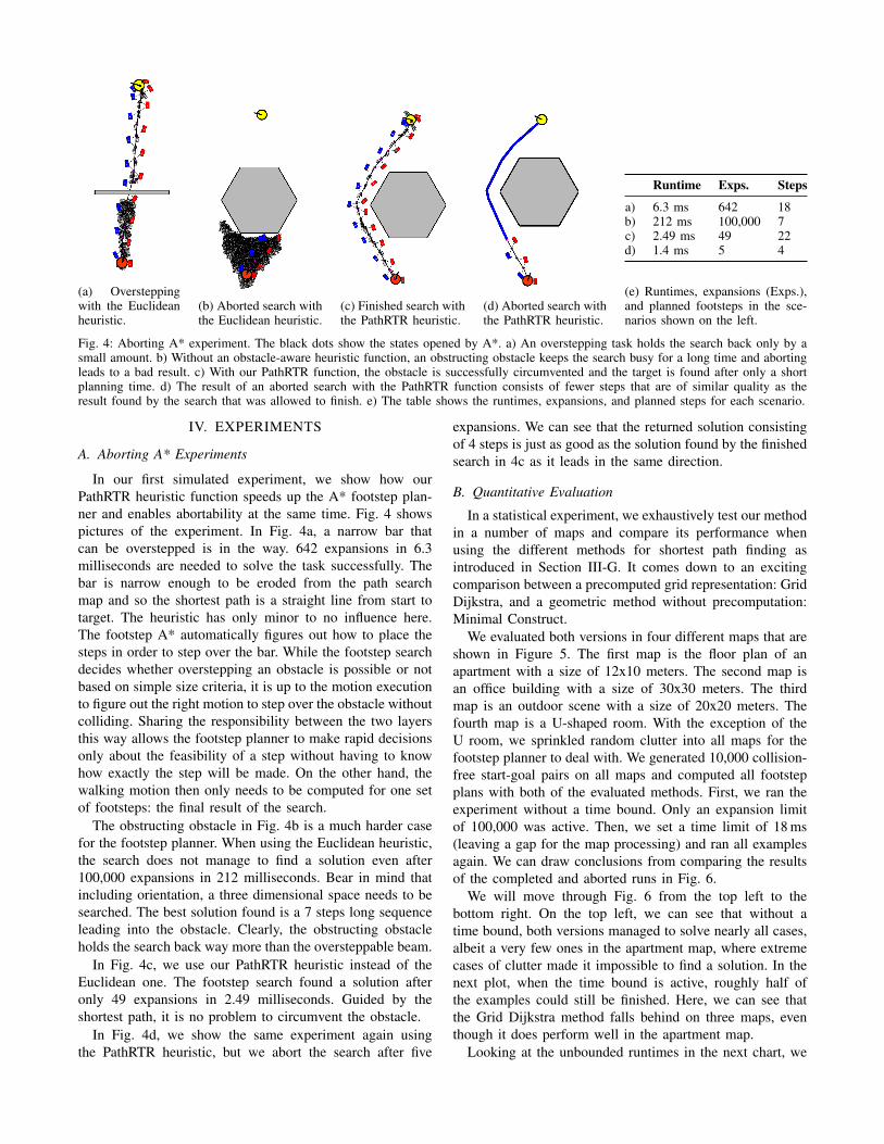
Fig. 4: Aborting A* experiment. The black dots show the states opened by A*. a) An overstepping task holds the search back only by asmall amount. b) Without an obstacle-aware heuristic function, an obstructing obstacle keeps the search busy for a long time and abortingleads to a bad result. c) With our PathRTR function, the obstacle is successfully circumvented and the target is found after only a shortplanning time. d) The result of an aborted search with the PathRTR function consists of fewer steps that are of similar quality as theresult found by the search that was allowed to finish. e) The table shows the runtimes, expansions, and planned steps for each scenario.
IV. EXPERIMENTS
A. Aborting A* Experiments
In our first simulated experiment, we show how ourPathRTR heuristic function speeds up the A* footstep plan-ner and enables abortability at the same time. Fig. 4 showspictures of the experiment. In Fig. 4a, a narrow bar thatcan be overstepped is in the way. 642 expansions in 6.3milliseconds are needed to solve the task successfully. Thebar is narrow enough to be eroded from the path searchmap and so the shortest path is a straight line from start totarget. The heuristic has only minor to no influence here.The footstep A* automatically figures out how to place thesteps in order to step over the bar. While the footstep searchdecides whether overstepping an obstacle is possible or notbased on simple size criteria, it is up to the motion executionto figure out the right motion to step over the obstacle withoutcolliding. Sharing the responsibility between the two layersthis way allows the footstep planner to make rapid decisionsonly about the feasibility of a step without having to knowhow exactly the step will be made. On the other hand, thewalking motion then only needs to be computed for one setof footsteps: the final result of the search.
The obstructing obstacle in Fig. 4b is a much harder casefor the footstep planner. When using the Euclidean heuristic,the search does not manage to find a solution even after100,000 expansions in 212 milliseconds. Bear in mind thatincluding orientation, a three dimensional space needs to besearched. The best solution found is a 7 steps long sequenceleading into the obstacle. Clearly, the obstructing obstacleholds the search back way more than the oversteppable beam.
In Fig. 4c, we use our PathRTR heuristic instead of theEuclidean one. The footstep search found a solution afteronly 49 expansions in 2.49 milliseconds. Guided by theshortest path, it is no problem to circumvent the obstacle.
In Fig. 4d, we show the same experiment again usingthe PathRTR heuristic, but we abort the search after five
expansions. We can see that the returned solution consistingof 4 steps is just as good as the solution found by the finishedsearch in 4c as it leads in the same direction.
B. Quantitative Evaluation
In a statistical experiment, we exhaustively test our methodin a number of maps and compare its performance whenusing the different methods for shortest path finding asintroduced in Section III-G. It comes down to an excitingcomparison between a precomputed grid representation: GridDijkstra, and a geometric method without precomputation:Minimal Construct.
We evaluated both versions in four different maps that areshown in Figure 5. The first map is the floor plan of anapartment with a size of 12x10 meters. The second map isan office building with a size of 30x30 meters. The thirdmap is an outdoor scene with a size of 20x20 meters. Thefourth map is a U-shaped room. With the exception of theU room, we sprinkled random clutter into all maps for thefootstep planner to deal with. We generated 10,000 collision-free start-goal pairs on all maps and computed all footstepplans with both of the evaluated methods. First, we ran theexperiment without a time bound. Only an expansion limitof 100,000 was active. Then, we set a time limit of 18 ms(leaving a gap for the map processing) and ran all examplesagain. We can draw conclusions from comparing the resultsof the completed and aborted runs in Fig. 6.
We will move through Fig. 6 from the top left to thebottom right. On the top left, we can see that without atime bound, both versions managed to solve nearly all cases,albeit a very few ones in the apartment map, where extremecases of clutter made it impossible to find a solution. In thenext plot, when the time bound is active, roughly half ofthe examples could still be finished. Here, we can see thatthe Grid Dijkstra method falls behind on three maps, eventhough it does perform well in the apartment map.
Looking at the unbounded runtimes in the next chart, we

Fig. 5: Artificially generated maps that we used for statistical experiments. Left: a 12x10 meters large apartment (Apt). Left middle: a30x30 meters large office building (Off). Right middle: a 20x20 meters large outdoor scene (Out). Right: The U room (U).
0%
25%
50%
75%
100%
Min. Const. Grid Dijk.
Finished Cases (no limit)
AptOff
OutU
0%
25%
50%
75%
100%
Min. Const. Grid Dijk.
Finished Cases (aborted)
AptOff
OutU
0
50
100
150
200
250
Min. Const. Grid Dijk.
Runtime in ms (no limit)
AptOff
OutU
0 5
10 15 20 25 30 35 40
Min. Const. Grid Dijk.
Runtime in ms (aborted)
AptOff
OutU
5K
10K
15K
20K
25K
Min. Const. Grid Dijk.
A* Expansions (no limit)
AptOff
OutU
0
500
1000
1500
2000
2500
Min. Const. Grid Dijk.
A* Expansions (aborted)
AptOff
OutU
0
10
20
30
40
50
60
Min. Const. Grid Dijk.
Planned Steps (no limit)
AptOff
OutU
0
10
20
30
40
50
60
Min. Const. Grid Dijk.
Planned Steps (aborted)
AptOff
OutU
Fig. 6: Charts of the Minimal Construct and the Grid Dijkstra versions of our footstep planner performing on the Apartment map (Apt),the Office map (Off), the Outdoor map (Out), and the U room (U).
can see that the footstep plans typically finish in under 100milliseconds on all maps. The Grid Dijkstra method needsa little more time to finish than its geometric counterparteven though the portion of time spent on the precomputation,this is marked in orange color in the bar stack, seems ratherinsignificant. In the next plot, the aborted times are shown.Both methods manage to stay below the 20 millisecondsmark, even though the Minimal Construct method a littlemore so than the Grid Dijkstra version. We can see thatthe map computation part shown in red at the bottom ofthe bar stack is only a fraction of the time needed for thesearch. The precomputation time for the Dijkstra table shownin orange, however, is now quite significant. Notably, thisprecomputation time is much smaller on the apartment mapwhere often a large portion of the local map is blocked spaceor outside of the global map and, thus, less cells need to beprocessed. We measured the runtimes on a laptop with anIntel Core5 i5-7200U 4 x 2.50GHz CPU.
In the next plot, the number of expansions of the unabortedruns shows that when using the grid, significantly more stepsneed to be expanded to find the target. This is interestingsince the geometric and the grid methods compute almost thesame shortest paths. The only difference between them is thediscretization of the Dijkstra table, which is enough to disturbthe search this much. The number of expansions of theaborted searches in the next plot show that the precomputedDijkstra grid profits from the faster lookups and manages to
expand more steps in the same amount of time as the graphmethods, even though this does not help solving more cases.
Finally, if we then look at the number of steps in theresulting footstep plans in the last two charts, it comes asa surprise that the average lengths of the resulting plansare nearly the same whether the search is aborted or not.Consequently, the quality of the plans found with a bounded-time search cannot be far behind the completed plans.
Additionally, we provide a demonstration video1 of ouralgorithm replanning during walking at a frequency of 50 Hz.
V. CONCLUSIONSIn conclusion, we proposed a fast footstep planner that is
capable of quickly computing footstep plans in a local maparound the robot with a guaranteed bound on the runtime.This way, footstep planning becomes feasible even for a low-level motion controller running at 50 Hz. We were able toboost the speed of footstep planning using a novel PathRTRheuristic function combined with the shortest path to thegoal, which not only speeds up the search in the presenceof obstacles, but also allows us to abort an A* searchprematurely with a good solution. In future work, we areplanning to extend our footstep planner with Capture Stepcapabilities [29] that are directly included in the footstepplan. We are also planning to account for moving objectsand to extend our planning capabilities to 3D.
1Video: https://youtu.be/EI9mHx0uxLU

REFERENCES
[1] Robert J. Griffin, Georg Wiedebach, Stephen McCrory, SylvainBertrand, Inho Lee, and Jerry Pratt. Footstep planning for autonomouswalking over rough terrain. In Proc. of the IEEE/RAS Int. Conf. onHumanoid Robots (Humanoids), 2019.
[2] J. Kuffner, K. Nishiwaki, S. Kagami, and M. Inaba. Footstep planningamong obstacles for biped robots. In Proc. of the IEEE/RSJ Int. Conf.on Intelligent Robots & Systems (IROS), 2001.
[3] J. Kuffner, S. Kagami, K. Nishiwaki, M. Inaba, and H. Inoue. Onlinefootstep planning for humanoid robots. In IEEE Int. Conf. on Roboticsand Automation (ICRA), 2003.
[4] J. Chestnutt, M. Lau, K.M. Cheung, J. Kuffner, J.K. Hodgins, andT. Kanade. Footstep planning for the Honda ASIMO humanoid. InIEEE Int. Conf. on Robotics and Automation (ICRA), 2005.
[5] Y. Ayaz, K. Munawar, M.B. Malik, A. Konno, and M. Uchiyama.Human-like approach to footstep planning among obstacles for hu-manoid robots. In Proc. of the IEEE/RSJ Int. Conf. on IntelligentRobots & Systems (IROS), 2006.
[6] Armin Hornung, Andrew Dornbush, Maxim Likhachev, and MarenBennewitz. Anytime search-based footstep planning with suboptimal-ity bounds. In Proc. of the IEEE-RAS International Conference onHumanoid Robots (HUMANOIDS), 2012.
[7] Armin Hornung, Daniel Maier, and Maren Bennewitz. Search-basedfootstep planning. In Proc. of the ICRA Workshop on Progress andOpen Problems in Motion Planning and Navigation for Humanoids,2013.
[8] P.E. Hart, N.J. Nilsson, and B. Raphael. A formal basis for the heuristicdetermination of minimum cost paths. IEEE Trans. on Systems,Science, and Cybernetics, SSC-4(2):100–107, 1968.
[9] M. Likhachev, D. Ferguson, G. Gordon, A. Stentz, and S. Thrun. Any-time search in dynamic graphs. Artificial Intelligence, 172(14):1613– 1643, 2008.
[10] Maxim Likhachev and Anthony Stentz. R* search. In Proc. of theNational Conference on Artificial Intelligence (AAAI), pages 344–350,2008.
[11] Armin Hornung and Maren Bennewitz. Adaptive level-of-detailplanning for efficient humanoid navigation. In Proc. of the IEEE Int.Conf. on Robotics & Automation (ICRA), 2012.
[12] Johannes Garimort, Armin Hornung, and Maren Bennewitz. Hu-manoid navigation with dynamic footstep plans. In Proc. of the IEEEInt. Conf. on Robotics & Automation (ICRA), 2011.
[13] S. Koenig and M. Likhachev. D∗ Lite. In Proc. of the NationalConference on Artificial Intelligence (AAAI), 2002.
[14] Scott Kuindersma, Robin Deits, Maurice Fallon, Andres Valenzuela,Hongkai Dai, Frank Permenter, Twan Koolen, Pat Marion, and RussTedrake. Optimization-based locomotion planning, estimation, andcontrol design for the Atlas humanoid robot. Autonomous Robots,40(3):429–455, 2016.
[15] Dimitrios Kanoulas, Alexander Stumpf, Vignesh Sushrutha Raghavan,Chengxu Zhou, Alexia Toumpa, Oskar von Stryk, Darwin G. Caldwell,and Nikos G. Tsagarakis. Footstep planning in rough terrain forbipedal robots using curved contact patches. In Proc. of the IEEEInt. Conf. on Robotics & Automation (ICRA), 2018.
[16] Alexander Stumpf, Stefan Kohlbrecher, David C. Conner, and Oskarvon Stryk. Supervised footstep planning for humanoid robots in roughterrain tasks using a black box walking controller. In Proc. of theIEEE/RAS Int. Conf. on Humanoid Robots (Humanoids), 2014.
[17] S. Feng, X. Xinjilefu, C. G. Atkeson, and J. Kim. Optimization basedcontroller design and implementation for the Atlas robot in the DARPArobotics challenge finals. In Proc. of the IEEE/RAS Int. Conf. onHumanoid Robots (Humanoids), 2015.
[18] S. Feng, X. Xinjilefu, C. G. Atkeson, and J. Kim. Robust dynamicwalking using online foot step optimization. In Proc. of the IEEE/RSJInt. Conf. on Intelligent Robots & Systems (IROS), 2016.
[19] R. Deits and R. Tedrake. Footstep planning on uneven terrain withmixed-integer convex optimization. In Proc. of the IEEE/RAS Int.Conf. on Humanoid Robots (Humanoids), 2014.
[20] Arne-Christoph Hildebrandt, Robert Wittmann, Felix Sygulla, DanielWahrmann, Daniel Rixen, and Thomas Buschmann. Versatile androbust bipedal walking in unknown environments: real-time collisionavoidance and disturbance rejection. Autonomous Robots, 43, 2019.
[21] A. C. Hildebrandt, D. Wahrmann, R. Wittmann, D. Rixen, andT. Buschmann. Real-time pattern generation among obstacles for bipedrobots. In Proc. of the IEEE/RSJ Int. Conf. on Intelligent Robots &Systems (IROS), 2015.
[22] Daniel Wahrmann, Arne-Christoph Hildebrandt, Tamas Bates, RobertWittmann, Felix Sygulla, Philipp Seiwald, and Daniel Rixen. Vision-based 3d modeling of unknown dynamic environments for real-timehumanoid navigation. Int. J. Humanoid Robotics, 16(1), 2019.
[23] Arne-Christoph Hildebrandt, Robert Wittmann, Daniel Wahrmann,Alexander Ewald, and Thomas Buschmann. Real-time 3d collisionavoidance for biped robots. In Proc. of the IEEE/RSJ Int. Conf. onIntelligent Robots & Systems (IROS), 2014.
[24] Nicolas Perrin, Olivier Stasse, Leo Baudouin, Florent Lamiraux, andEiichi Yoshida. Fast humanoid robot collision-free footstep planningusing swept volume approximations. IEEE Transactions on Robotics,28(2), 2012.
[25] P. Karkowski, S. Oßwald, and M. Bennewitz. Real-time footstepplanning in 3d environments. In Proc. of the IEEE-RAS InternationalConference on Humanoid Robots (HUMANOIDS), 2016.
[26] Marcell Missura, Arindam Roychoudhury, and Maren Bennewitz.Polygonal perception for mobile robots. In Proc. of the IEEE/RSJInt. Conf. on Intelligent Robots & Systems (IROS), 2020.
[27] Marcell Missura, Daniel D. Lee, and Maren Bennewitz. Minimalconstruct: Efficient shortest path finding for mobile robots in polygonalmaps. In Proc. of the IEEE/RSJ Int. Conf. on Intelligent Robots &Systems (IROS), 2018.
[28] A. Nash, S. Koenig, and Craig A. Tovey. Lazy Theta*: Any-anglepath planning and path length analysis in 3D. In Proc. of the NationalConference on Artificial Intelligence (AAAI), 2010.
[29] Marcell Missura, Maren Bennewitz, and Sven Behnke. Capture steps:Robust walking for humanoid robots. Int. J. Humanoid Robotics,16(6):1950032:1–1950032:28, 2019.