fast space-varying convolution using matrix source coding

1

Fast Space-Varying Convolution Using MatrixSource Coding

Jianing Wei,Member, IEEE,Charles A. Bouman,Fellow, IEEE,and Jan P. Allebach,Fellow, IEEE

Abstract—Many imaging applications require the implemen-tation of space-varying convolution for accurate restoration andreconstruction of images. Moreover, these space-varying convo-lution operators are often dense, so direct implementationofthe convolution operator is typically computationally impractical.One such example is the problem of stray light reduction in digitalcameras, which requires the implementation of a dense space-varying deconvolution operator. However, other inverse problems,such as iterative tomographic reconstruction, can also depend onthe implementation of dense space-varying convolution. Whilespace-invariant convolution can be efficiently implemented withthe Fast Fourier Transform (FFT), this approach does not workfor space-varying operators. So direct convolution is often theonly option for implementing space-varying convolution.

In this paper, we develop a general approach to the efficientimplementation of space-varying convolution, and demonstrateits use in the application of stray light reduction. Our approach,which we call matrix source coding, is based on lossy sourcecoding of the dense space-varying convolution matrix. Impor-tantly, by coding the transformation matrix, we not only reducethe memory required to store it; we also dramatically reducethe computation required to implement matrix-vector products.Our algorithm is able to reduce computation by approximatelyfactoring the dense space-varying convolution operator into aproduct of sparse transforms. Experimental results show thatour method can dramatically reduce the computation requiredfor stray light reduction while maintaining high accuracy.

Index Terms—Stray light, space-varying point spread func-tion, image restoration, fast algorithm, inverse problem,digitalphotography.

I. INTRODUCTION

In many important imaging applications, it is useful tomodel the acquired data vector,y, as

y = Ax + w, (1)

wherex is the unknown image to be determined,A is a lineartransformation matrix, andw is some additive noise that isindependent ofx with inverse covarianceΛw. This simplelinear model can capture many important inverse problemsincluding image deblurring [1], tomographic reconstruction[2], and super-resolution [3].

This research work was done when Jianing Wei was a Ph.D. student atthe Department of Electrical and Computer Engineering, Purdue University.Jianing Wei is with US Research Center, Sony Electronics Inc., San Jose,CA 95112, USA. Charles A. Bouman and Jan P. Allebach are with theSchool of Electrical and Computer Engineering, Purdue University, WestLafayette, IN 47906, USA. Email: [email protected],{bouman, alle-bach}@purdue.edu.

This material is based upon work supported by, or in part by, the U. S. ArmyResearch Laboratory and the U. S. Army Research Office under contract/grantnumber 56541-CI, and the National Science Foundation underContract CCR-0431024.

There is a vast literature related to the effective solutionofinverse problems with the form of Eq. (1). Solution to theseinverse problems can be very difficult if the transformationsAor AtΛwA are ill conditioned. This can and often does happenif the data is sparse or of low quality. In these cases, manyalgorithms have been proposed to recoverx from y. Classicalapproaches include algebraic reconstruction techniques (ART)[4]; simultaneous iterative reconstruction technique (SIRT) [5];simultaneous algebraic reconstruction technique (SART) [6];Lucy-Richardson algorithm [7]; Van Cittert’s method [1], [8];approximate [9] or true [10] maximum likelihood estimation;regularized inversion [11]; and maximum a posteriori (MAP)inversion [12], [13], [14]. A common objective in all thesemethods is to balance the goal of matching the observed (butnoisy) data with the goal of producing a physically realisticimage.

While many methods exist for addressing the inverse prob-lem of Eq. (1), all these methods typically require the com-putation of matrix-vector products, such asAx, or Aty. Infact, iterative inversion methods typically require the repeatedcomputation of the matrix-vector productAtAx or AtΛwAx.If the matrix A is sparse, as is the case with a differentialoperator [15], or if it can be decomposed as a product ofsparse transformations, as is the case with the wavelet [16]or fast Fourier transform (FFT) [17], then computation ofAxis fast and tractable. For example, ifAx is space-invariantconvolution, thenA can be decomposed as the product of twoFFTs and a diagonal transform, resulting in a total computationfor the evaluation ofAx that has an order ofO(P log P )where P is the size ofx. However, if A represents space-varying convolution with a large point-spread function, theneach direct evaluation of the matrix-vector productAx orAty can require enormous computation. Even whenAtA isapproximately Toeplitz, as is often the case in tomographicreconstruction [4], the matrixAtΛwA will not be Toeplitzwhen the noise is space varying.

The specific application considered in this paper is thatof stray light reduction for digital photographs [18]. Straylight refers to the portion of the entering light flux that ismisdirected to undesired locations in the image plane. It issometimes referred to as lens flare or veiling glare [19]. It canbe caused by imperfections in lens elements, or reflectionsbetween optical surfaces; but in the end, it tends to reducethe contrast of images by scattering light from bright regionsof the image into dark regions. Since stray light is typicallyscattered across the imaging field, its associated point spreadfunction (PSF) typically has large support and is space-varying

2

[18]. With this in mind, an imaging system with stray lightcan be modeled using Eq. (1) with

A = (1 − β)I + βS, (2)

whereI is the identity matrix,S is a dense matrix describingthe space-varying scattering of light across the imaging array1,andβ is a scalar constant representing the fraction of scatteredlight.

Typically the fraction of scattered light is small, and weknow that the matrixA is very well conditioned, so in contrastto many inverse problems, stray light reduction is a well-posedinverse problem, and the solution can be computed using aformula such as that proposed by Jansson and Fralinger [20]

x = (1 + β)y − βSy, (3)

wherey is the observed image, andx is the estimate of theunderlying image to be recovered.

However, even in this simple form, the computation ofEq. (3) is not practical for a modern digital camera, becausethe matrix S is both dense and lacks a Toeplitz structure.In typical stray light models, the PSF is space-varying withheavy tails, so the FFT cannot be directly used to speed upcomputation [18]. For example, if the image containsP pixels,the computation isO(P 2); so for a106 pixel image, it takes106 multiplies to compute each output pixel, resulting in a totalof 1012 multiplies. This much computation requires hours ofprocessing time, which makes accurate stray light reductioninfeasible for implementation in low cost digital cameras.

In this paper, we propose a novel algorithm for fast com-putation of space-varying convolution, and we demonstrateits effectiveness for the particular application of stray lightreduction. Our method, which we refer to as matrix sourcecoding (MSC), is based on the use of lossy source codingtechniques to compress the dense matrixS into a sparse form.Importantly, the effect of this compression is not only to reducethe memory required for storingS, but also to dramaticallyreduce the number of multiplies required to approximatelycompute the matrix-vector productSy. Our approach worksby first decorrelating the rows and columns ofS and thenquantizing the resulting compacted matrix so that most of itsentries become zero.

Our MSC method requires both on-line and off-line compo-nents. While the on-line component is fast, it requires the pre-computation of a sparse matrix decomposition in an off-lineprocedure. We introduce a method for efficiently implementingthis off-line computation for a broad class of space-varyingkernels whose wavelet coefficients are localized in space.

In order to assess the value of our approach, we apply it tothe problem of stray light reduction for digital cameras. Usingthe stray light model of [18], we demonstrate that the MSCmethod can achieve an accuracy of 1% with approximately7 multiplies per pixel at image resolution1024 × 1024, adramatic reduction when compared to direct space-varyingconvolution. We also demonstrate a practical pre-computaion

1Due to conservation of energy, we know that the columns ofS sum toless than 1.

algorithm that can be performed in time proportion to thekernel size.

In Section II we introduce the MSC method. The on-line algorithm for space-varying convolution is derived andpresented in Section II-A, and the off-line pre-computationmethod is presented in Section II-B and Section IV. Section IIIpresents the stray light application and model, and SectionVfollows with experimental results. Section VI concludes thispaper.

II. M ATRIX SOURCE CODING APPROACH TO

SPACE-VARYING CONVOLUTION

In this section, we present the matrix source coding (MSC)approach for fast space-varying convolution. The MSC ap-proach has two parts, which we will refer to as the on-lineand off-line computations. The on-line algorithm computesthespace-varying convolution using a product of sparse matrices.Section II-A presents the on-line algorithm along with itsassociated theory.

While the on-line computation is very fast, it depends onthe result of off-line computation, which is to pre-computea sparse version of the original space-varying convolutionmatrix. This computation is not input image-dependent, andonly depends on the PSF of the imaging system. However,naive computation of this sparse matrix can be enormouslycomputationally demanding. So in Section II-B, we introducean efficient algorithm for accurate but approximate computa-tion of the required sparse transformation for a broad classofproblems.

A. Matrix Source Coding Theory

Our goal is to speed up the computation of general matrix-vector products with the form

z = Sy,

where y is the input, z is the output, andS is a denseP × P matrix without a Toeplitz structure.2 If S is Toeplitz,then Sy can be efficiently computed using the fast Fouriertransform (FFT) [21]. However, whenS implements space-varying convolution, then it is not Toeplitz; and the FFT cannotbe used directly.

Our strategy for speeding up computation ofSy is to uselossy transform coding of the rows and columns ofS. Theresulting coded matrix then becomes sparse after quantiza-tion, and this sparsity reduces both storage and computation.However, in order to perform lossy source coding ofS, wemust first determine the relevant distortion metric.

In general, the mean squared error (MSE) is not a gooddistortion metric for codingS because it does not account forany correlation in the vectory. In order to see this, let[S]be a quantized version ofS produced by lossy coding anddecoding. Then the distortion introduced into the outputz isgiven by

δz = S y − [S] y = δS y,

2In fact, all our results hold whenS is a non-squareP1 × P2 matrix.However, we consider the special case ofP = P1 = P2 here for notationalsimplicity. The extension to the more general case is direct.

3

whereδS = S−[S] is the distortion introduced intoS throughlossy coding andδz is the resulting distortion introduced intoz. Using the argument of [22], [23] and assuming thaty isindependent ofδS, then the expected MSE inδz is given by

E[

‖δz‖2|δS]

= E[

trace{δzδzt}|δS]

= E[

trace{δSyytδSt}|δS]

= trace{δS E[

yyt|δS]

δSt}

= trace{δS Ry δSt},

whereRy = E[yyt] = E [yyt|δS]. Notice that in the specialcase wheny is white, then we have thatRy = I, and

E[

‖δz‖2|δS]

= ‖δS‖2 . (4)

In other words, when the inputy is white, minimizing thesquared error distortion of the matrixS (i.e. the Frobeniusnorm) is equivalent to minimizing the expected value of thesquared error distortion forz. However, when the componentsof y are correlated, then minimum MSE coding ofS can bequite far from minimizing the MSE inz.

Based on this result, our strategy for source-coding ofS willbe to first transform the matrixS so its input is white, and itsrows and columns are decorrelated; and then to quantize thetransformed matrix so it becomes sparse. More specifically,we define the transformed matrixS as

S = W1ST−1, (5)

whereW1 is an orthonormal transform3 andT is an invertibletransform. Then the outputz can be computed as

z = W−11 ST y . (6)

Our objective is then to select the matricesT andW1 so thatT whitens (i.e. spheres) the covariance ofy, and together,T and W1 deorrelate the rows and columns ofS. Since thecovariance ofTy is whitened and the rows and columns ofS are decorrelated, we can apply MMSE quantization ofS inorder to achieve MMSE estimation ofz. So if [S] denotes thequantized version ofS, then we have that

z = W−11 [S]Ty , (7)

wherez is the approximation ofz.Given that the rows and columns ofS are approximately

decorrelated, then we should expect that the quantized matrix,[S], will be sparse, and that therefore, multiplying with[S]will be computationally efficient and, just as importantly,[S]will be easy to store. However, in practice, if the transformsTandW1 are dense, then the application of these decorrelatingtransforms might require as much computation as the originalmultiplication byS. This would, of course, defeat the purposeof the sparsification ofS.

In fact, the “optimal” decorrelating transforms,T andW1,have exactly this property. Appendix A constructs transformsT and W1 that exactly achieve the goal of whitening (i.e.sphereing)y and decorrelating the rows and columns (i.e.diagonalizing) ofS. This can be done by selectingT as the

3Without loss of generality, these transforms can be orthogonal, but fornotional simplicity we also assume they are normal.

Fig. 1. Block diagram of on-line computation of matrix source coding.

generalized eigendecomposition of the matrix pair(Ry , Rc ,

StS) [21] and by selectingW1 as the eigendecompositionfor the covariance matrixRr , SSt. However, while this“optimal” choice produces perfect decorrelation and sparsity,it is not practical because the transformsT andW1 are then,in general, dense transformations with no fast implementation.

So our objective is to find computationally efficient trans-formations forT andW1 which approximately whiteny anddecorrelate the rows and columns ofS. In order to achievethis objective, we will use wavelet transforms to decorrelateboth the vectory, and the rows and columns ofS. The wavelettransform is a reasonable choice because it is known to be anapproximation to the Karhunen-Loeve transform for stationarysources [24], and it is commonly used as a decorrelatingtransform for various source coding applications [25]. Usingthis strategy, we form the matrixT by a wavelet transformfollowed by gain factors designed to normalize the varianceof wavelet coefficients. This combination of decorrelationandscaling whitens or spheres the vectory. Specifically, we choose

T = Λ−1/2w W2, (8)

where W2 is a wavelet transform andΛ−1/2w is a diagonal

matrix of gain factors so that

Λw = diag(

W2RyW t2

)

, (9)

whereRy = E[yyt] is the covariance ofy. At the same time,notice that the transformT−1 = W−1

2 Λ1/2w approximately

decorrelates the columns ofS.4 Similarly, if we choose thetransformW1 to be a wavelet transform, then it will alsodecorrelate the rows ofS, so that [S] will be sparse afterquantization.

To summarize, Fig. 1 illustrates a block diagram of the on-line computation required for matrix source coding of Eq. (7).First, the input datay is transformed and scaled. Then itis multiplied by a sparse matrix[S]. Then a second inversewavelet transform is applied to compute the approximateresult z. The accuracy of the approximation is determinedby the degree of quantization applied toS. So if little or noquantization is used, then the computation can be arbitrarilyclose to exact, but at the cost of less sparsity inS and thereforemore computation and storage. In this way, matrix sourcecoding allows for a continuous tradeoff between accuracy andcomputation/storage.

Finally, as a practical matter, the diagonal matrixΛw can beeasily estimated from training images. In fact, we will assumethat the gain factors for each subband are constant since thewavelet coefficients in the same subband typically have thesame variance [1]. So to estimateΛw, we take the wavelet

4This is true because if theS is slowly space-varying operator, then thecovariance matrixRr = StS is approximately Toeplitz; and the wavelettransform approximates the Karhunen-Loeve transform.

4

transformW2 of the training images, compute the varianceof the wavelet coefficients in each subband, and average overall images to obtain an estimate of the gain factors for eachsubband.

B. Efficient Off-Line Computation for Matrix Source Coding

In order to implement the fast space-varying convolutionmethod described by Eq. (7), it is first necessary to computethe source coded matrix[S]. We will refer to the computationof [S] as the off-line portion of the computation. Once thesparse matrix[S] is available, then the space-varying convo-lution may be efficiently computed using on-line computationshown in Eq. (7).

However, even though the computation of[S] is performedoff-line, exact evaluation of this sparse matrix is still too largefor practical problems. For example, if the image contains16million pixels, then temporary storage ofS requires approx-imately 106 Giga bytes of memory, exceeding the capacityof modern computers. The following section describes anefficient approach to compute[S] which eliminates the needfor any such temporary storage.

In our implementation, we use the Haar wavelet transform[16] for both W1 andW2. The Haar wavelet transform is anorthonormal transform, so we have that

S = W1ST−1

= W1SW t2Λ1/2

w .

Therefore, direct implementation of this off-line computationconsists of a wavelet transformW2 along the rows ofS,scaling of the matrix entries, and a wavelet transformW1 alongthe columns. Unfortunately, the computational complexityofthese two operations isO(P 2), whereP is the number ofpixels in the image, because the operation requires that eachentry ofS be touched. This computation can take a tremendousamount of time for high resolution images. Therefore, weaim at reducing the computational complexity to be linearlyproportional toP and eliminating the need to store the entirematrix S. In order to achieve this goal, we will use a twostage quantization procedure combined with a recursive top-down algorithm for computing the Haar wavelet transformcoefficients.

The first stage of this procedure is to zero out the entriesin SW t

2Λ1/2w whose magnitudes are less than a specified

threshold. We useQt(SW t2Λ

1/2w ) to describe this thresholding

stage, where for a scalarx

Qt(x) =

{

x for |x| > t0 otherwise

. (10)

The resulting matrixQt(SW t2Λ

1/2w ) is already quite sparse,

thus there is no need to store the entire dense matrix. Thenthe second stage of this procedure is to compute the wavelettransformW1 over the columns of this already sparse matrix.Taking advantage of the sparsity resulting from the first stage,if the average number of remaining nonzero entries in eachrow of Qt(SW t

2Λ1/2w ) is N (N ≪ P ), then the computation

of the wavelet transform in the second stage is reduced from

O(P 2) to O(NP ). In summary, this two stage procedure isexpressed mathematically as

[S] ≈ [W1Qt(SW t2Λ1/2

w )]. (11)

However, there is still a problem as to how to efficientlycomputeQt(SW t

2Λ1/2w ). SinceS is dense, direct evaluation

of this expression requiresO(P 2) operations. However, afterthresholding, most values inQt(SW t

2Λ1/2w ) are zero, so we

can dramatically reduce computation by first identifying theregions where non-zero values are likely to occur. We referto these non-zero values as significant wavelet coefficients.As mentioned before, we useN to denote the number ofsignificant wavelet coefficients per row. Once we can predictthe location of the significant wavelet coefficients, we can use arecursive top-down approach to compute them without havingto do the full wavelet transform for each row ofS. We willdiscuss how to predict the location of the significant waveletcoefficients in constant time in Sec. IV.

Next, we describe our algorithm for computing the signif-icant wavelet coefficients once their location is known. Ourstrategy is to first compute the approximation coefficients thatare necessary to compute the significant wavelet coefficientsusing a recursive top-down approach. Then significant detailcoefficients can be computed from the approximation coef-ficients at finer resolutions. Our approach is able to achieveO(N) computational complexity for computing the significantHaar wavelet coefficients per row, which leads to a totalcomplexity ofO(NP ) for computingQt(SW t

2Λ1/2w ).

We usef(k, i, j) to represent the approximation coefficientat location(i, j) at level k, where larger values ofk corre-spond to coarser scales, andf(0, i, j) corresponds to the fullresolution image. We usegh(k, i, j), gv(k, i, j), andgd(k, i, j)to represent the detail coefficients in horizontal, vertical anddiagonal bands, respectively. We can then computef(k, i, j) asthe average of its corresponding 4 higher resolution neighbors:

f(k, i, j) =1

2(f(k − 1, 2i, 2j) + f(k − 1, 2i + 1, 2j)

+f(k − 1, 2i, 2j + 1) + f(k − 1, 2i + 1, 2j + 1)).

(12)

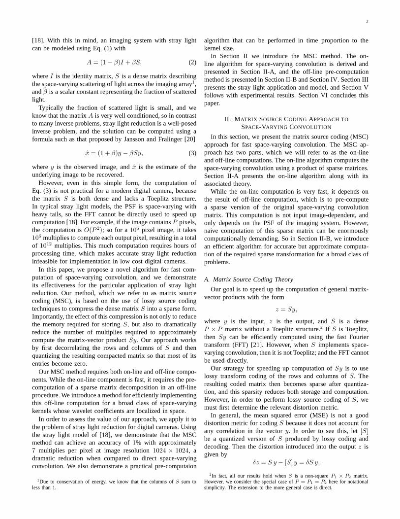
Equation (12) specifies the parent/child relations of a quad-treeas shown in Figure 2. Our algorithm transverses this quad-tree in a pruned depth-first search; and at each step of thesearch, the corresponding wavelet approximation coefficient iscomputed. The search is pruned whenever the wavelet detailcoefficients are determined to be “insignificant”. In this case,the wavelet approximation coefficient is directly approximatedby the local value of the actual image using the relationship

f(k, i, j) ≈ 2kf(0, 2ki, 2kj). (13)

When the search is not pruned, then the wavelet approximationcoefficient is computed using Eq. (12), where the finer resolu-tion coefficients are evaluated using recursion. Of course,wealso terminate the search whenk = 0 since this is the finestresolution at which the wavelet approximation coefficient canbe evaluated exactly. Figure 2 provides a graphic illustrationof how the search transverses from the coarsest to finest

5

k + 1

k

k − 1

Fig. 2. An illustration of the quad-tree structure of Haar approximationcoefficients. Dark gray squares are internal nodes of the pruned quad-tree.Corresponding detail coefficients are significant at these nodes, and we go onto the next level recursion. Light gray squares are leaf nodes of the prunedquad-tree. The termination condition of our recursive algorithm is met at thesenodes; so the values are directly computed and returned. Empty squares arenodes pruned off from the quad-tree. Values at these nodes are not computedor touched.

resolutions, and Fig. 3 provides a more precise pseudo-codespecification of the algorithm.

After obtaining the necessary approximation coefficients,we can compute the significant detail coefficients using thefollowing equations:

gh(k, i, j) =1

2(f(k − 1, 2i, 2j)− f(k − 1, 2i, 2j + 1)

+f(k − 1, 2i + 1, 2j) − f(k − 1, 2i + 1, 2j + 1)),

gv(k, i, j) =1

2(f(k − 1, 2i, 2j) + f(k − 1, 2i, 2j + 1)

−f(k − 1, 2i + 1, 2j) − f(k − 1, 2i + 1, 2j + 1)),

gd(k, i, j) =1

2(f(k − 1, 2i, 2j)− f(k − 1, 2i, 2j + 1)

−f(k − 1, 2i + 1, 2j) + f(k − 1, 2i + 1, 2j + 1)).

(14)

Notice that the complexity of our algorithm to computeQt(SW t

2Λ1/2w ) is O(NP ). To see that this is true, notice

that the total complexity of the depth-first search is linearlyproportional to the number of nodes in the tree, and thenumber of nodes in the tree is proportional toN . Moreover, thecomputation performed at each node has fixed computationalcomplexity because we have assumed that the subroutine Sig-nificantCoef of Fig. 3(c) has constant complexity. So puttingthis together, we know that the complexity of computing thewavelet transform for each row isO(N). Thus, the totalcomplexity of evaluating the wavelet transform forP rowsmust be orderO(NP ).

The second stage of our matrix source coding is awavelet transformW1 along the columns of the sparse matrixQt(SW t

2Λ1/2w ). Storing the entire sparse matrixQt(SW t

2Λ1/2w )

prior to computing the wavelet transformW1 may exceed thememory capacity of computers for high resolution images. Soin practice, we use block wavelet transforms forW1 to reducememory usage. In this way, we can perform the transformblock-by-block, and only need to keepQt(SW t

2Λ1/2w ) for

each block prior to computing wavelet transformW1. Oncethe transformW1 for a block is complete, the values in

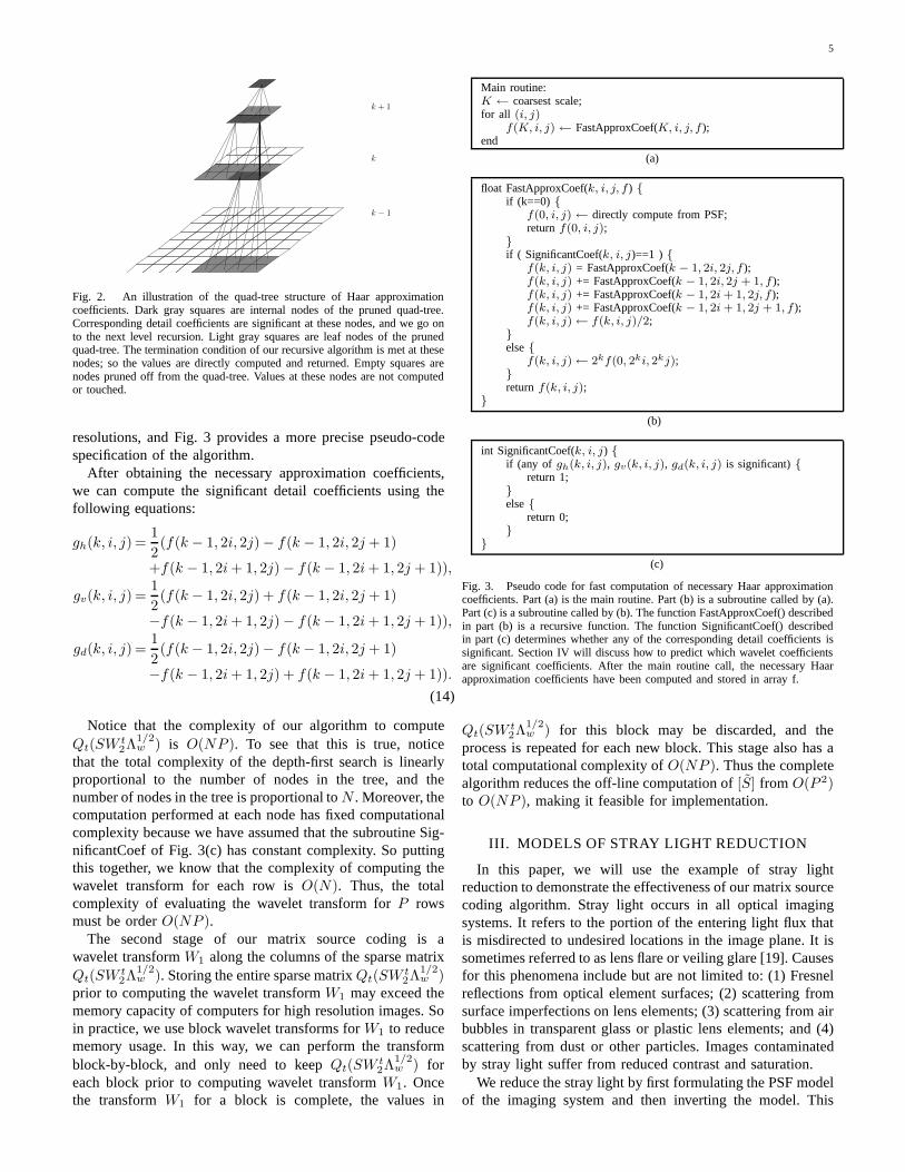
Main routine:K ← coarsest scale;for all (i, j)

f(K, i, j) ← FastApproxCoef(K, i, j, f );end

(a)

float FastApproxCoef(k, i, j, f ) {if (k==0) {

f(0, i, j) ← directly compute from PSF;returnf(0, i, j);

}if ( SignificantCoef(k, i, j)==1 ) {

f(k, i, j) = FastApproxCoef(k − 1, 2i, 2j, f );f(k, i, j) += FastApproxCoef(k − 1, 2i, 2j + 1, f );f(k, i, j) += FastApproxCoef(k − 1, 2i + 1, 2j, f );f(k, i, j) += FastApproxCoef(k − 1, 2i + 1, 2j + 1, f );f(k, i, j)← f(k, i, j)/2;

}else{

f(k, i, j)← 2kf(0, 2ki, 2kj);}returnf(k, i, j);

}

(b)

int SignificantCoef(k, i, j) {if (any of gh(k, i, j), gv(k, i, j), gd(k, i, j) is significant){

return 1;}else{

return 0;}

}

(c)

Fig. 3. Pseudo code for fast computation of necessary Haar approximationcoefficients. Part (a) is the main routine. Part (b) is a subroutine called by (a).Part (c) is a subroutine called by (b). The function FastApproxCoef() describedin part (b) is a recursive function. The function SignificantCoef() describedin part (c) determines whether any of the corresponding detail coefficients issignificant. Section IV will discuss how to predict which wavelet coefficientsare significant coefficients. After the main routine call, the necessary Haarapproximation coefficients have been computed and stored inarray f.

Qt(SW t2Λ

1/2w ) for this block may be discarded, and the

process is repeated for each new block. This stage also has atotal computational complexity ofO(NP ). Thus the completealgorithm reduces the off-line computation of[S] from O(P 2)to O(NP ), making it feasible for implementation.

III. MODELS OF STRAY LIGHT REDUCTION

In this paper, we will use the example of stray lightreduction to demonstrate the effectiveness of our matrix sourcecoding algorithm. Stray light occurs in all optical imagingsystems. It refers to the portion of the entering light flux thatis misdirected to undesired locations in the image plane. Itissometimes referred to as lens flare or veiling glare [19]. Causesfor this phenomena include but are not limited to: (1) Fresnelreflections from optical element surfaces; (2) scattering fromsurface imperfections on lens elements; (3) scattering from airbubbles in transparent glass or plastic lens elements; and (4)scattering from dust or other particles. Images contaminatedby stray light suffer from reduced contrast and saturation.

We reduce the stray light by first formulating the PSF modelof the imaging system and then inverting the model. This

6

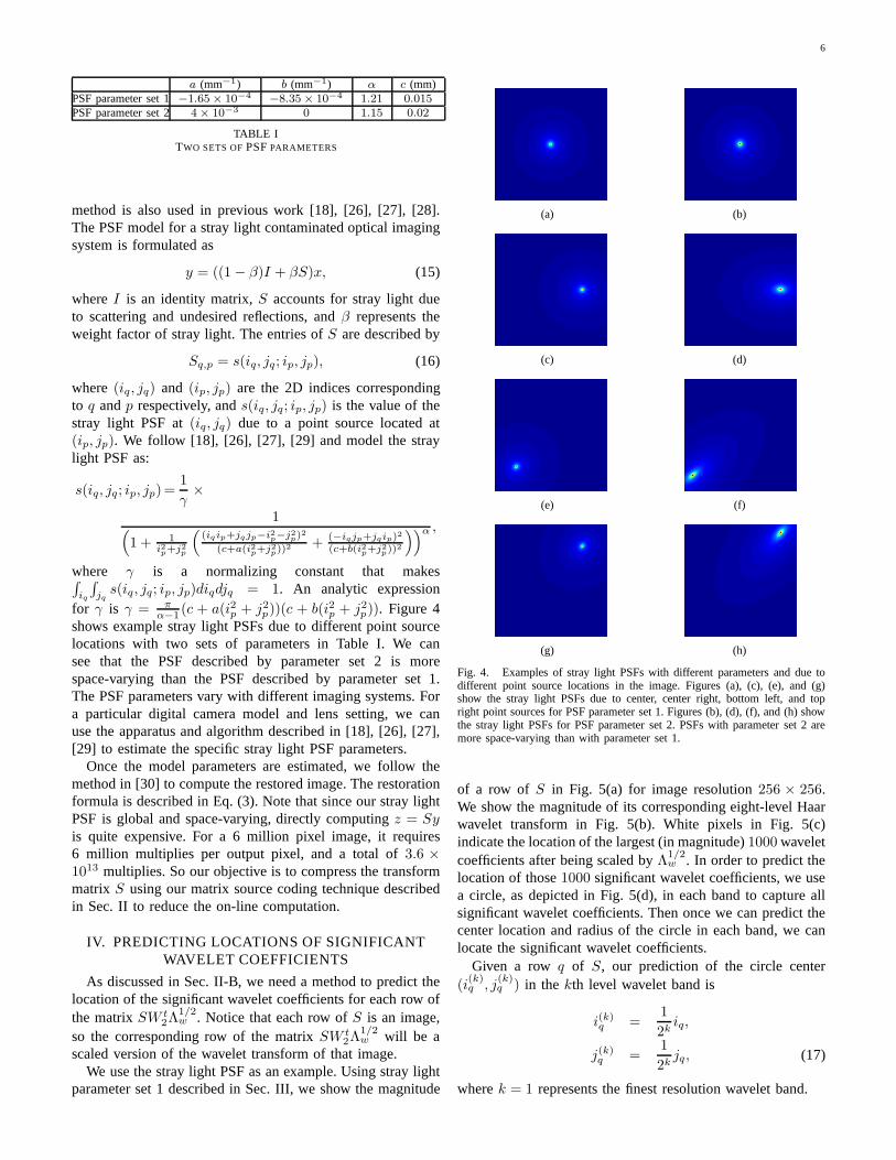
a (mm−1) b (mm−1) α c (mm)PSF parameter set 1−1.65× 10−4 −8.35× 10−4 1.21 0.015PSF parameter set 2 4× 10−3 0 1.15 0.02

TABLE ITWO SETS OFPSFPARAMETERS

method is also used in previous work [18], [26], [27], [28].The PSF model for a stray light contaminated optical imagingsystem is formulated as

y = ((1 − β)I + βS)x, (15)

whereI is an identity matrix,S accounts for stray light dueto scattering and undesired reflections, andβ represents theweight factor of stray light. The entries ofS are described by

Sq,p = s(iq, jq; ip, jp), (16)

where (iq, jq) and (ip, jp) are the 2D indices correspondingto q andp respectively, ands(iq, jq; ip, jp) is the value of thestray light PSF at(iq, jq) due to a point source located at(ip, jp). We follow [18], [26], [27], [29] and model the straylight PSF as:

s(iq, jq; ip, jp)=1

γ×

1(

1 + 1i2p+j2

p

(

(iqip+jqjp−i2p−j2

p)2

(c+a(i2p+j2

p))2 +

(−iqjp+jqip)2

(c+b(i2p+j2

p))2

))α ,

where γ is a normalizing constant that makes∫

iq

∫

jq

s(iq, jq; ip, jp)diqdjq = 1. An analytic expressionfor γ is γ = π

α−1 (c + a(i2p + j2p))(c + b(i2p + j2

p)). Figure 4shows example stray light PSFs due to different point sourcelocations with two sets of parameters in Table I. We cansee that the PSF described by parameter set 2 is morespace-varying than the PSF described by parameter set 1.The PSF parameters vary with different imaging systems. Fora particular digital camera model and lens setting, we canuse the apparatus and algorithm described in [18], [26], [27],[29] to estimate the specific stray light PSF parameters.

Once the model parameters are estimated, we follow themethod in [30] to compute the restored image. The restorationformula is described in Eq. (3). Note that since our stray lightPSF is global and space-varying, directly computingz = Syis quite expensive. For a 6 million pixel image, it requires6 million multiplies per output pixel, and a total of3.6 ×1013 multiplies. So our objective is to compress the transformmatrix S using our matrix source coding technique describedin Sec. II to reduce the on-line computation.

IV. PREDICTING LOCATIONS OF SIGNIFICANTWAVELET COEFFICIENTS

As discussed in Sec. II-B, we need a method to predict thelocation of the significant wavelet coefficients for each rowofthe matrixSW t

2Λ1/2w . Notice that each row ofS is an image,

so the corresponding row of the matrixSW t2Λ

1/2w will be a

scaled version of the wavelet transform of that image.We use the stray light PSF as an example. Using stray light

parameter set 1 described in Sec. III, we show the magnitude

(a) (b)

(c) (d)

(e) (f)

(g) (h)

Fig. 4. Examples of stray light PSFs with different parameters and due todifferent point source locations in the image. Figures (a),(c), (e), and (g)show the stray light PSFs due to center, center right, bottomleft, and topright point sources for PSF parameter set 1. Figures (b), (d), (f), and (h) showthe stray light PSFs for PSF parameter set 2. PSFs with parameter set 2 aremore space-varying than with parameter set 1.

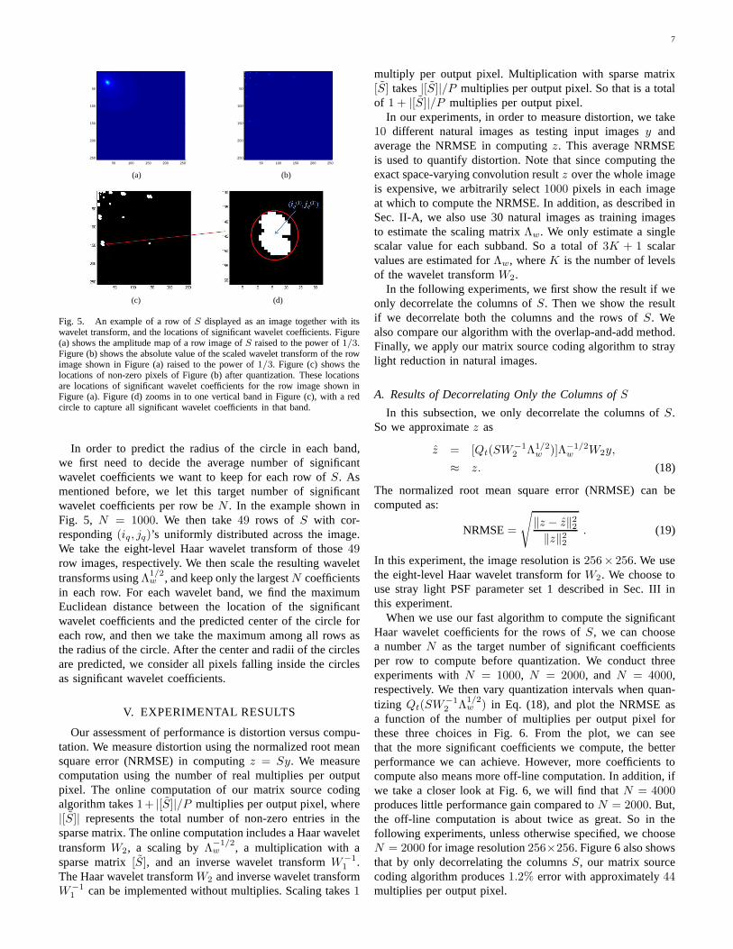
of a row of S in Fig. 5(a) for image resolution256 × 256.We show the magnitude of its corresponding eight-level Haarwavelet transform in Fig. 5(b). White pixels in Fig. 5(c)indicate the location of the largest (in magnitude)1000 waveletcoefficients after being scaled byΛ1/2

w . In order to predict thelocation of those1000 significant wavelet coefficients, we usea circle, as depicted in Fig. 5(d), in each band to capture allsignificant wavelet coefficients. Then once we can predict thecenter location and radius of the circle in each band, we canlocate the significant wavelet coefficients.

Given a row q of S, our prediction of the circle center(i

(k)q , j

(k)q ) in the kth level wavelet band is

i(k)q =

1

2kiq,

j(k)q =

1

2kjq, (17)

wherek = 1 represents the finest resolution wavelet band.

7

50 100 150 200 250

50

100

150

200

250

50 100 150 200 250

50

100

150

200

250

(a) (b)

(c) (d)

Fig. 5. An example of a row ofS displayed as an image together with itswavelet transform, and the locations of significant waveletcoefficients. Figure(a) shows the amplitude map of a row image ofS raised to the power of1/3.Figure (b) shows the absolute value of the scaled wavelet transform of the rowimage shown in Figure (a) raised to the power of1/3. Figure (c) shows thelocations of non-zero pixels of Figure (b) after quantization. These locationsare locations of significant wavelet coefficients for the rowimage shown inFigure (a). Figure (d) zooms in to one vertical band in Figure(c), with a redcircle to capture all significant wavelet coefficients in that band.

In order to predict the radius of the circle in each band,we first need to decide the average number of significantwavelet coefficients we want to keep for each row ofS. Asmentioned before, we let this target number of significantwavelet coefficients per row beN . In the example shown inFig. 5, N = 1000. We then take49 rows of S with cor-responding(iq, jq)’s uniformly distributed across the image.We take the eight-level Haar wavelet transform of those49row images, respectively. We then scale the resulting wavelettransforms usingΛ1/2

w , and keep only the largestN coefficientsin each row. For each wavelet band, we find the maximumEuclidean distance between the location of the significantwavelet coefficients and the predicted center of the circle foreach row, and then we take the maximum among all rows asthe radius of the circle. After the center and radii of the circlesare predicted, we consider all pixels falling inside the circlesas significant wavelet coefficients.

V. EXPERIMENTAL RESULTS

Our assessment of performance is distortion versus compu-tation. We measure distortion using the normalized root meansquare error (NRMSE) in computingz = Sy. We measurecomputation using the number of real multiplies per outputpixel. The online computation of our matrix source codingalgorithm takes1+ |[S]|/P multiplies per output pixel, where|[S]| represents the total number of non-zero entries in thesparse matrix. The online computation includes a Haar wavelettransformW2, a scaling byΛ

−1/2w , a multiplication with a

sparse matrix[S], and an inverse wavelet transformW−11 .

The Haar wavelet transformW2 and inverse wavelet transformW−1

1 can be implemented without multiplies. Scaling takes1

multiply per output pixel. Multiplication with sparse matrix[S] takes|[S]|/P multiplies per output pixel. So that is a totalof 1 + |[S]|/P multiplies per output pixel.

In our experiments, in order to measure distortion, we take10 different natural images as testing input imagesy andaverage the NRMSE in computingz. This average NRMSEis used to quantify distortion. Note that since computing theexact space-varying convolution resultz over the whole imageis expensive, we arbitrarily select1000 pixels in each imageat which to compute the NRMSE. In addition, as described inSec. II-A, we also use 30 natural images as training imagesto estimate the scaling matrixΛw. We only estimate a singlescalar value for each subband. So a total of3K + 1 scalarvalues are estimated forΛw, whereK is the number of levelsof the wavelet transformW2.

In the following experiments, we first show the result if weonly decorrelate the columns ofS. Then we show the resultif we decorrelate both the columns and the rows ofS. Wealso compare our algorithm with the overlap-and-add method.Finally, we apply our matrix source coding algorithm to straylight reduction in natural images.

A. Results of Decorrelating Only the Columns ofS

In this subsection, we only decorrelate the columns ofS.So we approximatez as

z = [Qt(SW−12 Λ1/2

w )]Λ−1/2w W2y,

≈ z. (18)

The normalized root mean square error (NRMSE) can becomputed as:

NRMSE=

√

‖z − z‖22

‖z‖22

. (19)

In this experiment, the image resolution is256× 256. We usethe eight-level Haar wavelet transform forW2. We choose touse stray light PSF parameter set 1 described in Sec. III inthis experiment.

When we use our fast algorithm to compute the significantHaar wavelet coefficients for the rows ofS, we can choosea numberN as the target number of significant coefficientsper row to compute before quantization. We conduct threeexperiments withN = 1000, N = 2000, and N = 4000,respectively. We then vary quantization intervals when quan-tizing Qt(SW−1

2 Λ1/2w ) in Eq. (18), and plot the NRMSE as

a function of the number of multiplies per output pixel forthese three choices in Fig. 6. From the plot, we can seethat the more significant coefficients we compute, the betterperformance we can achieve. However, more coefficients tocompute also means more off-line computation. In addition,ifwe take a closer look at Fig. 6, we will find thatN = 4000produces little performance gain compared toN = 2000. But,the off-line computation is about twice as great. So in thefollowing experiments, unless otherwise specified, we chooseN = 2000 for image resolution256×256. Figure 6 also showsthat by only decorrelating the columnsS, our matrix sourcecoding algorithm produces1.2% error with approximately44multiplies per output pixel.

8

15 20 25 30 35 40 45 50 550

0.01

0.02

0.03

0.04

0.05

0.06

number of multiplies per output pixel

NR

MS

E

N=1000N=2000N=4000

(a) Plot of NRMSE

40 42 44 46 48 500.008

0.01

0.012

0.014

0.016

0.018

0.02


NR

MS

E

N=1000N=2000N=4000

(b) Zoom in partial plot

Fig. 6. Plot of NRMSE as a function of the number of multipliesperoutput pixel using our matrix source coding algorithm, but only decorrelatingthe columns ofS. The green dashed line, the black solid line, and the bluedashed line represent the results when the target number of significant waveletcoefficients per rowN = 1000, N = 2000, and N = 4000, respectively.We can see that for the same number of multiplies per output pixel, increasingN reduces NRMSE, although the difference is small.

B. Results of Decorrelating Both the Columns and Rows ofS

In addition to decorrelating the columns, we also decorrelatethe rows with wavelet transformW1. Thenz is approximatedas

z = W−11 [W1Qt(SW t

2Λ1/2w )]Λ−1/2

w W2y,

≈ z. (20)

We use PSF parameter set 1, and plot in Fig. 7 the aver-age NRMSE against number of multiplies per output pixel,and compare it with the performance of decorrelating onlycolumns. We can see that to achieve1% error, decorrelatingonly columns requires approximately48 multiplies per outputpixel, whereas decorrelating both rows and columns requiresapproximately14 multiplies per output pixel. Therefore, thisexperiment demonstrates the significance of decorrelatingbothrows and columns of the matrixS.

In addition, to better understand the computational savings,we use two different image resolutions of256 × 256 and1024 × 1024 in our experiments. In both cases, we set thetarget number of significant wavelet coefficients per row tobe N = 2000. We use two sets of PSF parameters describedin Sec. III to conduct our experiments. In the1024 × 1024case, we use a ten-level Haar wavelet transform forW2 and

10 15 20 25 30 35 40 45 50 550

0.01

0.02

0.03

0.04

0.05

0.06


NR

MS

E

decorrelating columns onlydecorrelating both rows and columns

Fig. 7. Comparison of performance between decorrelating columns onlyand decorrelating both rows and columns. The black solid curve depicts theperformance of decorrelating columns only. The red dashed curve depicts theperformance of decorrelating both rows and columns.

a three-level block Haar wavelet transform forW1. We plotthe NRMSE against number of multiplies per output pixel inFig. 8. We can see that for PSF parameter set 1, at1024×1024resolution, with only1% error, our algorithm reduces thenumber of multiplies per output pixel from1048576 = 10242

to only 7, which is a149796 :1 reduction in computation. At256 × 256 resolution, to achieve the same accuracy, we needabout14 multiplies per output pixel. So our algorithm achievesa higher reduction in computation for higher resolutions. Inaddition, we find that the error for the1024 × 1024 casedoes not decrease much when the number of multiplies perpixel becomes large. That is because the error introduced inthe first stage quantizationQt(SW t

2Λ1/2w ) does not change for

different quantization intervals in the second stage. If wetry toreduce the error in the first stage by increasingN from 2000to 4000, we can see the difference in performance in Fig. 9,especially for the1024×1024 case. For the256×256 case, theperformance is almost the same forN = 2000 andN = 4000.This is because the error introduced in the first stage is almostidentical for N = 2000 and N = 4000, as shown in Fig. 6.But for the1024× 1024 case, the performance is boosted byincreasing the value ofN .

C. Comparison with Overlap-and-add Method

A conventional way to compute space-varying convolutionis to use the overlap-and-add method [31], [32]. This methodfirst partitions the input imagey into blocks, then computes theoutput for each block over a larger (overlapped) region, andfinally adds the results together to approximate the final outputimagez. The reason why it can be fast is that when computingthe output for each block, it assumes spatially invariant PSF forthat particular block, thus fast Fourier transform (FFT) can beused to significantly reduce computational complexity. Similarto our algorithm, this method also has a trade-off betweenspeed and accuracy. More block partitions will produce higheraccuracy, but requires more computation. The size of theoutput region for each block depends on the size of the blockand the spatial support of the PSF. If the block is of sizeh×h,and the PSF has a spatial support of(r+1)×(r+1), then the

9

5 10 15 20 250

0.005

0.01

0.015

0.02


NR

MS

E

image resolution 256x256image resolution 1024x1024

(a) PSF parameter set 1

4 6 8 10 12 140

0.005

0.01

0.015

0.02


NR

MS

E

image resolution 256x256image resolution 1024x1024

(b) PSF parameter set 2

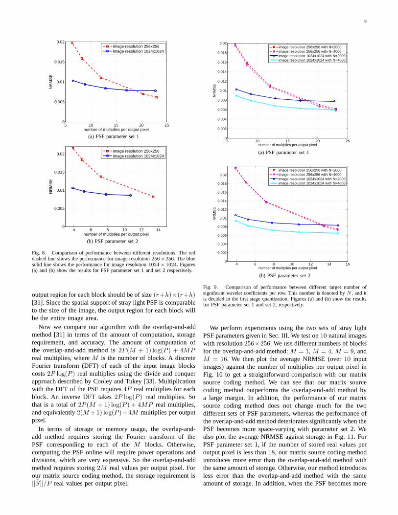
Fig. 8. Comparison of performance between different resolutions. The reddashed line shows the performance for image resolution256×256. The bluesolid line shows the performance for image resolution1024× 1024. Figures(a) and (b) show the results for PSF parameter set 1 and set 2 respectively.

output region for each block should be of size(r+h)×(r+h)[31]. Since the spatial support of stray light PSF is comparableto the size of the image, the output region for each block willbe the entire image area.

Now we compare our algorithm with the overlap-and-addmethod [31] in terms of the amount of computation, storagerequirement, and accuracy. The amount of computation ofthe overlap-and-add method is2P (M + 1) log(P ) + 4MPreal multiplies, whereM is the number of blocks. A discreteFourier transform (DFT) of each of the input image blockscosts2P log(P ) real multiplies using the divide and conquerapproach described by Cooley and Tukey [33]. Multiplicationwith the DFT of the PSF requires4P real multiplies for eachblock. An inverse DFT takes2P log(P ) real multiplies. Sothat is a total of2P (M + 1) log(P ) + 4MP real multiplies,and equivalently2(M +1) log(P )+4M multiplies per outputpixel.

In terms of storage or memory usage, the overlap-and-add method requires storing the Fourier transform of thePSF corresponding to each of theM blocks. Otherwise,computing the PSF online will require power operations anddivisions, which are very expensive. So the overlap-and-addmethod requires storing2M real values per output pixel. Forour matrix source coding method, the storage requirement is|[S]|/P real values per output pixel.

5 10 15 20 250

0.002

0.004

0.006

0.008

0.01

0.012

0.014

0.016

0.018

0.02


NR

MS

E

image resolution 256x256 with N=2000image resolution 256x256 with N=4000image resolution 1024x1024 with N=2000image resolution 1024x1024 with N=4000


4 6 8 10 12 14 160

0.002

0.004

0.006

0.008

0.01

0.012

0.014

0.016

0.018

0.02


NR

MS

E

image resolution 256x256 with N=2000image resolution 256x256 with N=4000image resolution 1024x1024 with N=2000image resolution 1024x1024 with N=4000


Fig. 9. Comparison of performance between different targetnumber ofsignificant wavelet coefficients per row. This number is denoted byN , and itis decided in the first stage quantization. Figures (a) and (b) show the resultsfor PSF parameter set 1 and set 2, respectively.

We perform experiments using the two sets of stray lightPSF parameters given in Sec. III. We test on10 natural imageswith resolution256×256. We use different numbers of blocksfor the overlap-and-add method:M = 1, M = 4, M = 9, andM = 16. We then plot the average NRMSE (over10 inputimages) against the number of multiplies per output pixel inFig. 10 to get a straightforward comparison with our matrixsource coding method. We can see that our matrix sourcecoding method outperforms the overlap-and-add method bya large margin. In addition, the performance of our matrixsource coding method does not change much for the twodifferent sets of PSF parameters, whereas the performance ofthe overlap-and-add method deteriorates significantly when thePSF becomes more space-varying with parameter set 2. Wealso plot the average NRMSE against storage in Fig. 11. ForPSF parameter set 1, if the number of stored real values peroutput pixel is less than18, our matrix source coding methodintroduces more error than the overlap-and-add method withthe same amount of storage. Otherwise, our method introducesless error than the overlap-and-add method with the sameamount of storage. In addition, when the PSF becomes more

10

0 100 200 300 400 500 600 7000

0.005

0.01

0.015

0.02


NR

MS

E

overlap−and−addmatrix source coding


0 100 200 300 400 500 600 7000

0.01

0.02

0.03

0.04

0.05

0.06

0.07

0.08


NR

MS

E



Fig. 10. Plots of NRMSE against the number of multiplies per output pixelfor both the overlap-and-add method and matrix source coding algorithm overtwo different PSF parameter sets. The green solid line showsthe result of theoverlap-and-add method. The red dashed line shows the result of matrix sourcecoding algorithm. The PSF using parameter set 2 is more space-varying thanthe PSF using parameter set 1.

space-varying in PSF parameter set 2, our matrix source cod-ing method introduces much less error than the overlap-and-add method with the same amount of storage. For example,with 5 real values stored per output pixel, our matrix sourcecoding method produces an error of approximately1.5%,whereas the overlap-and-add method produces an error ofapproximately6%.

In order to demonstrate the results more intuitively, we usethe PSF parameter set 2 provided in Sec. III, and computethe exact convolution of the stray light PSF with a sampleinput image shown in Fig. 12(a) at resolution256 × 256.The exact convolution result is shown in Fig. 12(b). We showthe approximation results using the overlap-and-add methodwith one partition, four partitions, and sixteen partitions inFig. 13 (a), (c), and (e) respectively. The absolute differenceimages between the approximation results and the ground truthin Fig. 12 (b) are shown in Fig. 13 (b), (d), and (f). TheNRMSE is9.89% for one partition,6.25% for four partitions,and 3.96% for sixteen partitions. We can see that the erroris much reduced by using more partitions. We then computethe approximation using our matrix source coding algorithmwith 15 multiplies per output pixel and show the result in

0 5 10 15 20 25 30 350.002

0.004

0.006

0.008

0.01

0.012

0.014

0.016

0.018

0.02

number of stored real values per output pixel

NR

MS

E



0 5 10 15 20 25 30 350

0.01

0.02

0.03

0.04

0.05

0.06

0.07

0.08


NR

MS

E



Fig. 11. Plots of NRMSE against storage for both the overlap-and-addmethod and matrix source coding algorithm over two different PSF parametersets. The green solid line shows the result of the overlap-and-add method. Thered dashed line shows the result of matrix source coding algorithm. The PSFusing parameter set 2 is more space-varying than the PSF using parameter set1.

(a) (b)

Fig. 12. A sample test image for space-varying convolution with stray lightPSF. Figure (a) shows an input image. Figure (b) shows the exact result of theinput image convolved with a space-varying stray light PSF with parametersset 2.

Fig. 13(g). The difference image between our approximationand the ground truth is shown in Fig. 13(h). The NRMSE is0.74%. This error is even less than the one achieved by theoverlap-and-add method with sixteen partitions, which needs608 multiplies per output pixel.

11

0

0.1

0.2

0.3

0.4

0.5

0.6

0.7

0.8

0.9

1

0

0.01

0.02

0.03

0.04

0.05

0.06

0.07

0.08

0.09

0.1

(a) (b)

0

0.1

0.2

0.3

0.4

0.5

0.6

0.7

0.8

0.9

1

0

0.01

0.02

0.03

0.04

0.05

0.06

0.07

0.08

0.09

0.1

(c) (d)

0

0.1

0.2

0.3

0.4

0.5

0.6

0.7

0.8

0.9

1

0

0.01

0.02

0.03

0.04

0.05

0.06

0.07

0.08

0.09

0.1

(e) (f)

0

0.1

0.2

0.3

0.4

0.5

0.6

0.7

0.8

0.9

1

0

0.01

0.02

0.03

0.04

0.05

0.06

0.07

0.08

0.09

0.1

(g) (h)

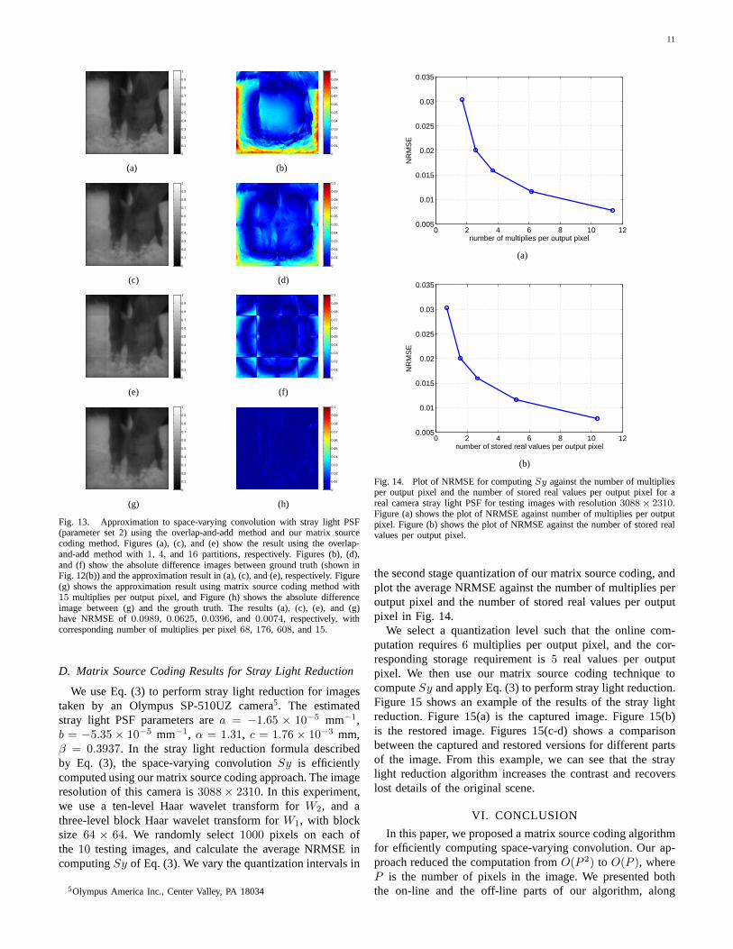
Fig. 13. Approximation to space-varying convolution with stray light PSF(parameter set 2) using the overlap-and-add method and our matrix sourcecoding method. Figures (a), (c), and (e) show the result using the overlap-and-add method with1, 4, and 16 partitions, respectively. Figures (b), (d),and (f) show the absolute difference images between ground truth (shown inFig. 12(b)) and the approximation result in (a), (c), and (e), respectively. Figure(g) shows the approximation result using matrix source coding method with15 multiplies per output pixel, and Figure (h) shows the absolute differenceimage between (g) and the grouth truth. The results (a), (c),(e), and (g)have NRMSE of0.0989, 0.0625, 0.0396, and 0.0074, respectively, withcorresponding number of multiplies per pixel68, 176, 608, and15.

D. Matrix Source Coding Results for Stray Light Reduction

We use Eq. (3) to perform stray light reduction for imagestaken by an Olympus SP-510UZ camera5. The estimatedstray light PSF parameters area = −1.65 × 10−5 mm−1,b = −5.35 × 10−5 mm−1, α = 1.31, c = 1.76 × 10−3 mm,β = 0.3937. In the stray light reduction formula describedby Eq. (3), the space-varying convolutionSy is efficientlycomputed using our matrix source coding approach. The imageresolution of this camera is3088 × 2310. In this experiment,we use a ten-level Haar wavelet transform forW2, and athree-level block Haar wavelet transform forW1, with blocksize 64 × 64. We randomly select1000 pixels on each ofthe 10 testing images, and calculate the average NRMSE incomputingSy of Eq. (3). We vary the quantization intervals in

5Olympus America Inc., Center Valley, PA 18034

0 2 4 6 8 10 120.005

0.01

0.015

0.02

0.025

0.03

0.035


NR

MS

E

(a)

0 2 4 6 8 10 120.005

0.01

0.015

0.02

0.025

0.03

0.035


NR

MS

E

(b)

Fig. 14. Plot of NRMSE for computingSy against the number of multipliesper output pixel and the number of stored real values per output pixel for areal camera stray light PSF for testing images with resolution 3088× 2310.Figure (a) shows the plot of NRMSE against number of multiplies per outputpixel. Figure (b) shows the plot of NRMSE against the number of stored realvalues per output pixel.

the second stage quantization of our matrix source coding, andplot the average NRMSE against the number of multiplies peroutput pixel and the number of stored real values per outputpixel in Fig. 14.

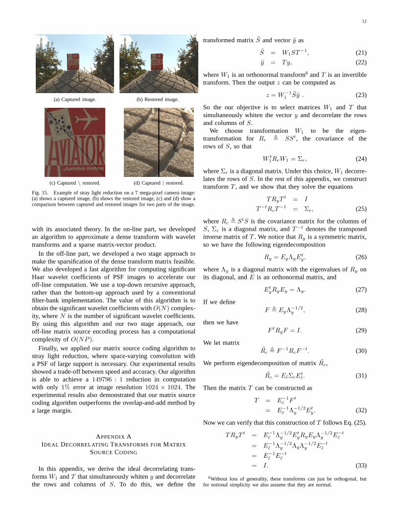
We select a quantization level such that the online com-putation requires6 multiplies per output pixel, and the cor-responding storage requirement is5 real values per outputpixel. We then use our matrix source coding technique tocomputeSy and apply Eq. (3) to perform stray light reduction.Figure 15 shows an example of the results of the stray lightreduction. Figure 15(a) is the captured image. Figure 15(b)is the restored image. Figures 15(c-d) shows a comparisonbetween the captured and restored versions for different partsof the image. From this example, we can see that the straylight reduction algorithm increases the contrast and recoverslost details of the original scene.

VI. CONCLUSION

In this paper, we proposed a matrix source coding algorithmfor efficiently computing space-varying convolution. Our ap-proach reduced the computation fromO(P 2) to O(P ), whereP is the number of pixels in the image. We presented boththe on-line and the off-line parts of our algorithm, along

12

(a) Captured image. (b) Restored image.

(c) Captured\ restored. (d) Captured| restored.

Fig. 15. Example of stray light reduction on a7 mega-pixel camera image:(a) shows a captured image, (b) shows the restored image, (c)and (d) show acomparison between captured and restored images for two parts of the image.

with its associated theory. In the on-line part, we developedan algorithm to approximate a dense transform with wavelettransforms and a sparse matrix-vector product.

In the off-line part, we developed a two stage approach tomake the sparsification of the dense transform matrix feasible.We also developed a fast algorithm for computing significantHaar wavelet coefficients of PSF images to accelerate ouroff-line computation. We use a top-down recursive approach,rather than the bottom-up approach used by a conventionalfilter-bank implementation. The value of this algorithm is toobtain the significant wavelet coefficients withO(N) complex-ity, whereN is the number of significant wavelet coefficients.By using this algorithm and our two stage approach, ouroff-line matrix source encoding process has a computationalcomplexity ofO(NP ).

Finally, we applied our matrix source coding algorithm tostray light reduction, where space-varying convolution witha PSF of large support is necessary. Our experimental resultsshowed a trade-off between speed and accuracy. Our algorithmis able to achieve a149796 : 1 reduction in computationwith only 1% error at image resolution1024 × 1024. Theexperimental results also demonstrated that our matrix sourcecoding algorithm outperforms the overlap-and-add method bya large margin.

APPENDIX AIDEAL DECORRELATINGTRANSFORMS FORMATRIX

SOURCE CODING

In this appendix, we derive the ideal decorrelating trans-formsW1 andT that simultaneously whiteny and decorrelatethe rows and columns ofS. To do this, we define the

transformed matrixS and vectory as

S = W1ST−1, (21)

y = Ty, (22)

whereW1 is an orthonormal transform6 andT is an invertibletransform. Then the outputz can be computed as

z = W−11 Sy . (23)

So the our objective is to select matricesW1 and T thatsimultaneously whiten the vectory and decorrelate the rowsand columns ofS.

We choose transformationW1 to be the eigen-transformation for Rr , SSt, the covariance of therows of S, so that

W t1RrW1 = Σr, (24)

whereΣr is a diagonal matrix. Under this choice,W1 decorre-lates the rows ofS. In the rest of this appendix, we constructtransformT , and we show that they solve the equations

TRyTt = I

T−tRcT−1 = Σc, (25)

whereRc , StS is the covariance matrix for the columns ofS, Σc is a diagonal matrix, andT−t denotes the transposedinverse matrix ofT . We notice thatRy is a symmetric matrix,so we have the following eigendecomposition

Ry = EyΛyEty, (26)

whereΛy is a diagonal matrix with the eigenvalues ofRy onits diagonal, andE is an orthonormal matrix, and

EtyRyEy = Λy. (27)

If we defineF , EyΛ−1/2

y , (28)

then we haveF tRyF = I. (29)

We let matrixRc , F−1RcF

−t. (30)

We perform eigendecomposition of matrixRc,

Rc = EcΣcEtc. (31)

Then the matrixT can be constructed as

T = E−1c F t

= E−1c Λ−1/2

y Ety. (32)

Now we can verify that this construction ofT follows Eq. (25).

TRyTt = E−1

c Λ−1/2y Et

yRyEyΛ−1/2y E−t

c

= E−1c Λ−1/2

y ΛyΛ−1/2y E−t

c

= E−1c E−t

c

= I. (33)

6Without loss of generality, these transforms can just be orthogonal, butfor notional simplicity we also assume that they are normal.

13

The last line of the above equation follows from the fact thatmatrix Ec is an orthonormal matrix, whose inverse is equal toits transpose. In addition,

T−tRcT−1 = Et

cF−1RcF

−tEc

= EtcRcEc

= Σc. (34)

So the matrixT from our construction fits Eq. (25). From ourconstruction, we can see that bothT and W1 are orthogonalmatrices. But they are not necessarily sparse or can be con-verted to sparse matrices. Therefore, these ideal decorrelatingmatrices are not useful in practice for the purpose of fastcomputation.

REFERENCES

[1] A. Bovik, Handbook of image and video processing. San Diego, CA:Academic Press, 2000.

[2] G. T. Herman and A. Kuba,Discrete Tomography: Foundations, Algo-rithms, and Applications. New York, NY: Birkhauser Boston, 1999.

[3] S. C. Park, M. K. Park, and M. G. Kang, “Super-resolution imagereconstruction: a technical overview,”IEEE Signal Processing Magazine,vol. 20, no. 3, pp. 21–36, May 2003.

[4] A. C. Kak and M. Slaney,Principles of Computerized TomographicImaging. Philadelphia, PA: Society for Industrial and Applied Mathe-matics, 2001.

[5] P. Gilbert, “Iterative methods for the three-dimensional reconstructionof an object from projections,”Journal of Theoretical Biology, vol. 36,no. 1, pp. 105–117, July 1972.

[6] A. H. Anderson and A. C. Kak, “Simultaneous algebraic reconstructiontechnique (SART): a superior implementation of the ART algorithm,”Ultrasonic Imaging, vol. 6, no. 1, pp. 81–94, January 1984.

[7] W. H. Richardson, “Bayesian-based iterative method of image restora-tion,” Journal of the Optical Society of America, vol. 62, no. 1, pp.55–59, 1972.

[8] P. H. V. Cittert, “Zum einfluss der spaltbreite auf die intensi-tatswerteilung in spektrallinien,”Z. Physik, vol. 69, pp. 298–308, 1931.

[9] H. M. Hudson and R. S. Larkin, “Accelerated image reconstructionusing ordered subsets of projection data,”IEEE Transactions on MedicalImaging, vol. 13, no. 4, pp. 601–609, 1994.

[10] L. A. Shepp and Y. Vardi, “Maximum likelihood reconstruction foremission tomography,”IEEE Transactions on Medical Imaging, vol. 2,pp. 113–122, 1982.

[11] A. N. Tychonoff and V. Y. Arsenin,Solution of Ill-posed Problems.Washington D. C.: V. H. Winston & Sons, January 1977.

[12] T. Hebert and R. Leahy, “A generalized EM algorithm for 3-D Bayesianreconstruction from Poisson data using Gibbs priors,”IEEE Transactionson Medical Imaging, vol. 8, pp. 194–202, 1989.

[13] P. J. Green, “Bayesian reconstruction from emission tomography datausing a modified EM algorithm,”IEEE Transactions on Medical Imag-ing, vol. 9, pp. 84–93, 1990.

[14] C. Bouman and K. Sauer, “A generalized gaussian image model for edge-preserving map estimation,”IEEE Transactions on Image Processing,vol. 2, no. 3, pp. 296–310, July 1993.

[15] C. Lanczos,Linear Differential Operators. Mineola, NY: DoverPublications, 1997.

[16] S. Mallat, A Wavelet Tour of Signal Processing. San Diego, CA:Academic Press, 1998.

[17] J. W. Cooley and J. W. Tukey, “An algorithm for the machine calculationof complex Fourier series,”Mathematics of Computation, vol. 19, no. 90,April 1965.

[18] J. Wei, B. Bitlis, A. Bernstein, A. Silva, P. A. Jansson,and J. P. Allebach,“Stray light and shading reduction in digital photography –a new modeland algorithm,” inProceedings of the SPIE/IS&T Conference on DigitalPhotography IV, vol. 6817, San Jose, CA, January 2008.

[19] W. J. Smith, Modern Optical Engineering : the Design of OpticalSystems. New York, NY: McGraw Hill, 2000.

[20] P. A. Jansson and J. H. Fralinger, “Parallel processingnetwork thatcorrects for light scattering in image scanners,”U.S. Patent 5,153,926,1992.

[21] G. H. Golub and C. F. V. Loan,Matrix Computations. Baltimore,Maryland: The Johns Hopkins University Press, 1996.

[22] G. Cao, C. A. Bouman, and K. J. Webb, “Fast and efficient stored matrixtechniques for optical tomography,” inProceedings of the 40th AsilomarConference on Signals, Systems, and Computers, October 2006.

[23] ——, “Results in non-iterative map reconstruction for optical tomogra-phy,” in Proceedings of the SPIE/IS&T Conference on ComputationalImaging VI, vol. 6814, San Jose, CA, January 2008.

[24] D. Tretter and C. A. Bouman, “Optimal transforms for multispectraland multilayer image coding,”IEEE Transactions on Image Processing,vol. 4, no. 3, pp. 296–308, 1995.

[25] D. Taubman and M. Marcellin,JPEG2000: Image Compression Fun-damentals, Standards and Practice. Norwell, MA: Kluwer AcademicPublishers, 2002.

[26] B. Bitlis, P. A. Jansson, and J. P. Allebach, “Parametric point spreadfunction modeling and reduction of stray light effects in digital stillcameras,” inProceedings of the SPIE/IS&T Conference on Computa-tional Imaging VI, vol. 6498, San Jose, CA, January 2007.

[27] P. A. Jansson, “Method, program, and apparatus for efficiently removingstray-flux effects by selected-ordinate image processing,” U.S. Patent6,829,393, 2004.

[28] J. Wei, G. Cao, C. A. Bouman, and J. P. Allebach, “Fast space-varyingconvolution and its application in stray light reduction,”in Proceedingsof the SPIE/IS&T Conference on Computational Imaging VII, vol. 7246,San Jose, CA, February 2009.

[29] P. A. Jansson and R. P. Breault, “Correcting color-measurement errorcaused by stray light in image scanners,” inProceedings of the SixthColor Imaging Conference: Color Science, Systems, and Applications,Scottsdale, AZ, November 1998.

[30] P. A. Jansson,Deconvolution of Images and Spectra. New York, NY:Academic Press, 1996.

[31] J. G. Nagy and D. P. O’Leary, “Fast iterative image restoration with aspatially varying PSF,” inProceedings of SPIE Conference on AdvancedSignal Processin g: Algorithms, Architectures, and Implementations VII,vol. 3162, San Diego, CA, 1997, pp. 388–399.

[32] J. Bardsley, S. Jefferies, J. Nagy, and R. Plemmons, “A computationalmethod for the restoration of images with an unknown, spatially-varyingblur,” Optics Express, vol. 15, no. 5, pp. 1767–1782, 2006.

[33] P. S. R. Diniz, E. A. B. da Silva, and S. L. Netto,Digital SignalProcessing System Analysis and Design. New York, NY: CambridgeUniversity Press, 2002.

fast space-varying convolution using matrix source coding

Documents