Fault Tolerant Multitenant DatabaseServer Consolidation

by

Joseph Mate

A thesispresented to the University of Waterloo

in fulfillment of thethesis requirement for the degree of

Master of Mathematicsin

Computer Science

Waterloo, Ontario, Canada, 2016

c© Joseph Mate 2016

brought to you by COREView metadata, citation and similar papers at core.ac.uk

provided by University of Waterloo's Institutional Repository

Author’s Declaration

This thesis consists of material all of which I authored or co-authored: see Statement of Con-tributions included in the thesis. This is a true copy of the thesis, including any required finalrevisions, as accepted by my examiners.

I understand that my thesis may be made electronically available to the public.

ii

Statement of Contributions

I would like to acknowledge the names of my co-authors who contributed to the research de-scribed in this dissertation, these include:

• Dr. Khuzaima Daudjee

• Dr. Shahin Kamali

• Fiodar Kazhamiaka

iii

Abstract

Server consolidation is important in situations where a sequence of database tenants needto be allocated (hosted) dynamically on a minimum number of cloud server machines. Givena tenant’s load defined by the amount of resources that the tenant requires and a service-level-agreement (SLA) between the tenant customer and the cloud service provider, resource costsavings can be achieved by consolidating multiple database tenants on server machines. Ad-ditionally, in realistic settings, server machines might fail causing their tenants to become un-available. To address this, service providers place multiple replicas of each tenant on differentservers and reserve extra capacity to ensure that tenant failover will not result in overload onany remaining server. The focus of this thesis is on providing effective strategies for placingtenants on server machines so that the SLA requirements are met in the presence of failure ofone or more servers. We propose the Cube-Fit (CUBEFIT) algorithm for multitenant databaseserver consolidation that saves resource costs by utilizing fewer servers than existing approachesfor analytical workloads. Additionally, unlike existing consolidation algorithms, CUBEFIT cantolerate multiple server failures while ensuring that no server becomes overloaded. We provideextensive theoretical analysis and experimental evaluation of CUBEFIT. We show that comparedto existing algorithms, the average case and worst case behavior of CUBEFIT is superior and thatCUBEFIT produces near-optimal tenant allocation when the number of tenants is large. Throughevaluation and deployment on a cluster of up to 73 machines as well as through simulation stud-ies, we experimentally demonstrate the efficacy of CUBEFIT in practical settings.

iv

Acknowledgements

I would like to thank Professor Wojciech Golab and Professor Tamer Ozsu for improving the con-tent and presentation of my thesis. Secondly, I would like to thank Dr. Shahin Kamali for lendinghis expertise on the theoretical aspect of the problem. Third, thank you Fiodar Kazhamiaka foryour help with CPLEX. Most of all, I must thank Professor Khuzaima Daudjee for guiding methrough all the obstacles in creating this thesis and for the extra effort he took to take my writingto a whole new level.

v

Table of Contents

Author’s Declaration ii

Statement of Contributions iii

Abstract iv

Acknowledgements v

List of Tables viii

List of Figures ix

1 Introduction 1

1.1 Background and Contributions . . . . . . . . . . . . . . . . . . . . . . . . . . . 3

1.2 Problem . . . . . . . . . . . . . . . . . . . . . . . . . . . . . . . . . . . . . . . 5

1.3 Online Bin Packing . . . . . . . . . . . . . . . . . . . . . . . . . . . . . . . . . 6

2 Background and Related Work 9

2.1 Goals and Approaches . . . . . . . . . . . . . . . . . . . . . . . . . . . . . . . 11

2.2 Failure Models . . . . . . . . . . . . . . . . . . . . . . . . . . . . . . . . . . . 13

2.3 Implementation Details . . . . . . . . . . . . . . . . . . . . . . . . . . . . . . . 14

vi

3 Cube-Fit Algorithm 16

3.1 Average-case Complexity . . . . . . . . . . . . . . . . . . . . . . . . . . . . . . 20

3.1.1 Uniform Distribution . . . . . . . . . . . . . . . . . . . . . . . . . . . . 20

3.1.2 Zipfian Distribution . . . . . . . . . . . . . . . . . . . . . . . . . . . . . 25

3.2 Worst-case Analysis . . . . . . . . . . . . . . . . . . . . . . . . . . . . . . . . . 26

4 System Model 29

5 Experiments 31

5.1 Robust Fit Interleaved . . . . . . . . . . . . . . . . . . . . . . . . . . . . . . . . 31

5.2 System Performance . . . . . . . . . . . . . . . . . . . . . . . . . . . . . . . . 32

5.2.1 Server Failures . . . . . . . . . . . . . . . . . . . . . . . . . . . . . . . 34

5.3 Simulations . . . . . . . . . . . . . . . . . . . . . . . . . . . . . . . . . . . . . 35

5.4 Comparison with Optimal . . . . . . . . . . . . . . . . . . . . . . . . . . . . . . 37

5.5 Sensitivity Experiments . . . . . . . . . . . . . . . . . . . . . . . . . . . . . . . 39

6 Conclusion and Future Work 45

References 46

APPENDICES 49

A Details of the Robust Fit Interleaved Algorithm 50

B Conversion of the Server Consolidation Problem to a Mixed Integer Program 54

B.1 Integer Program Formulation . . . . . . . . . . . . . . . . . . . . . . . . . . . . 54

B.2 Conversion to Mixed Integer Program . . . . . . . . . . . . . . . . . . . . . . . 55

C Small Improvement Due to Large Tenants 57

D CUBEFIT Optimizations 59

vii

List of Tables

2.1 Goals and Approaches of Multitenant Database Server Consolidation . . . . . . . 12

2.2 Failure Models of Multitenant Databases . . . . . . . . . . . . . . . . . . . . . . 13

2.3 Implementation Details of Multitenant Database Server Consolidation . . . . . . 15

3.1 Upper bounds for average ratio of CUBEFIT (with sufficiently large parameterK) when tenant sizes follow Zipfian distribution with different parameters s andM . . . . . . . . . . . . . . . . . . . . . . . . . . . . . . . . . . . . . . . . . . . 26

5.1 Yearly cost savings of CUBEFIT over RFI . . . . . . . . . . . . . . . . . . . . . 37

5.2 Comparison of the number of servers used by CUBEFIT, RFI, and CPLEX withthe given distributions using the maximum number of tenants solvable by CPLEX. 39

viii

List of Figures

1.1 A valid packing with two replica tenants and another packing with three replicas . 7

3.1 The first stage of CUBEFIT . . . . . . . . . . . . . . . . . . . . . . . . . . . . . 17

3.2 The idea behind CUBEFIT for placing replicas of the same type . . . . . . . . . . 18

3.3 A solution for an instance of upright matching . . . . . . . . . . . . . . . . . . . 23

4.1 Shared DBMS model: Tenants 1, 2 and 3 share the data store on the server. . . . 29

5.1 CUBEFIT and RFI placing 309 tenants, each with tenant load drawn from a dis-crete uniform distribution . . . . . . . . . . . . . . . . . . . . . . . . . . . . . . 32

5.2 CUBEFIT and RFI placing 1573 tenants, each with tenant load drawn from aZipfian distribution . . . . . . . . . . . . . . . . . . . . . . . . . . . . . . . . . 33

5.3 99th percentile latency of CUBEFIT and RFI with discrete uniform distributiontenants . . . . . . . . . . . . . . . . . . . . . . . . . . . . . . . . . . . . . . . . 34

5.4 99th percentile latency of CUBEFIT and RFI with Zipfian distribution tenants . . 35

5.5 % Relative difference of servers used by CubeFit over RFI for various uniformdistributions . . . . . . . . . . . . . . . . . . . . . . . . . . . . . . . . . . . . . 36

5.6 % Relative difference of servers used by CubeFit over RFI for various Zipfiandistributions . . . . . . . . . . . . . . . . . . . . . . . . . . . . . . . . . . . . . 37

5.7 % Relative difference of servers used by CubeFit over various class parametersusing uniform distribution . . . . . . . . . . . . . . . . . . . . . . . . . . . . . 41

5.8 % Relative difference of servers used by CubeFit over various class parametersusing Zipfian distributions . . . . . . . . . . . . . . . . . . . . . . . . . . . . . 42

ix

5.9 The minimum number of Uniformly distributed tenants needed until CubeFitalways performed better than RFI for various classes . . . . . . . . . . . . . . . 43

5.10 The minimum number of Zipfian distributed tenants needed until CubeFit alwaysperformed better than RFI for various classes . . . . . . . . . . . . . . . . . . . 44

A.1 Using RFI algorithm for placing a sequence of tenant replicas . . . . . . . . . . . 51

D.1 % Relative difference of servers used by optimized and αK versions of CubeFitusing uniform distributions . . . . . . . . . . . . . . . . . . . . . . . . . . . . . 60

D.2 % Relative difference of servers used by optimized and αK versions of CubeFitusing Zipfian distributions . . . . . . . . . . . . . . . . . . . . . . . . . . . . . 60

D.3 % Relative difference of servers used by optimized versus multi-tenants in thelast class versions of CubeFit using uniform distributions . . . . . . . . . . . . . 60

D.4 % Relative difference of servers used by optimized versus multi-tenants in thelast class versions of CubeFit using Zipfian distributions . . . . . . . . . . . . . 60

x

Chapter 1

Introduction

Cloud computing has transformed the information technology sector by providing software-as-a-service (SaaS) and infrastructure-as-a-service (IaaS) on demand. Cloud service providers, suchas Amazon Web Services [1], host client applications and their data on their cloud servers. Thisrelieves customers from technical tasks such as system operation, maintenance and provisioningof hardware resources. In a typical SaaS system, performance service level agreements (SLAs),agreed between clients and the service provider, define the minimum performance requirementfor software. The objective of a service provider is to meet the SLA requirement and, at thesame time, minimize the operational cost involved in providing such service. There is generallya trade-off between performance as perceived by customers, and the operational costs associatedwith using resources.

Cloud providers commonly consolidate client applications, called tenants, on shared com-puting resources to improve utilization and, as a result, reduce operating and maintenance costs.A service provider should have effective strategies for assigning or allocating tenants to reducethe number of servers (machines) that host tenants. This is critical for avoiding server sprawlin which there are numerous under-utilized active servers which consume more resources thanrequired by tenants. Preventing server sprawl is particularly important for green computing andsaving on the energy-related costs which account for 70 to 80 percent of a data center’s ongoingoperational costs [9].

To meet SLA requirements, server consolidation should be performed in a way such thatservers are not overloaded. Data centers usually have a large number of machines with homoge-neous server resources, providing significant resource capacity [24]. Similarly, each tenant has aload defined as the minimum amount of server compute resources required by the tenant to meetits SLA. If a server is overloaded, i.e., the total tenant load that it hosts exceed its capacity then

1

the SLA requirements will not be satisfied.

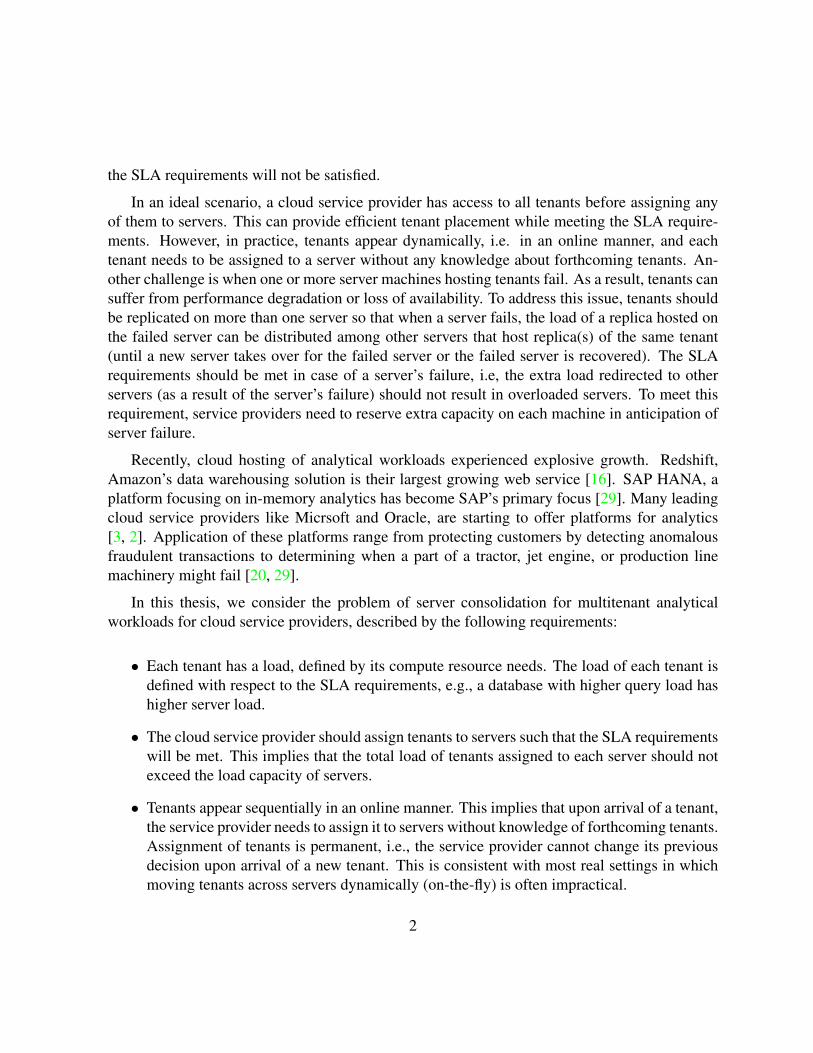
In an ideal scenario, a cloud service provider has access to all tenants before assigning anyof them to servers. This can provide efficient tenant placement while meeting the SLA require-ments. However, in practice, tenants appear dynamically, i.e. in an online manner, and eachtenant needs to be assigned to a server without any knowledge about forthcoming tenants. An-other challenge is when one or more server machines hosting tenants fail. As a result, tenants cansuffer from performance degradation or loss of availability. To address this issue, tenants shouldbe replicated on more than one server so that when a server fails, the load of a replica hosted onthe failed server can be distributed among other servers that host replica(s) of the same tenant(until a new server takes over for the failed server or the failed server is recovered). The SLArequirements should be met in case of a server’s failure, i.e, the extra load redirected to otherservers (as a result of the server’s failure) should not result in overloaded servers. To meet thisrequirement, service providers need to reserve extra capacity on each machine in anticipation ofserver failure.

Recently, cloud hosting of analytical workloads experienced explosive growth. Redshift,Amazon’s data warehousing solution is their largest growing web service [16]. SAP HANA, aplatform focusing on in-memory analytics has become SAP’s primary focus [29]. Many leadingcloud service providers like Micrsoft and Oracle, are starting to offer platforms for analytics[3, 2]. Application of these platforms range from protecting customers by detecting anomalousfraudulent transactions to determining when a part of a tractor, jet engine, or production linemachinery might fail [20, 29].

In this thesis, we consider the problem of server consolidation for multitenant analyticalworkloads for cloud service providers, described by the following requirements:

• Each tenant has a load, defined by its compute resource needs. The load of each tenant isdefined with respect to the SLA requirements, e.g., a database with higher query load hashigher server load.

• The cloud service provider should assign tenants to servers such that the SLA requirementswill be met. This implies that the total load of tenants assigned to each server should notexceed the load capacity of servers.

• Tenants appear sequentially in an online manner. This implies that upon arrival of a tenant,the service provider needs to assign it to servers without knowledge of forthcoming tenants.Assignment of tenants is permanent, i.e., the service provider cannot change its previousdecision upon arrival of a new tenant. This is consistent with most real settings in whichmoving tenants across servers dynamically (on-the-fly) is often impractical.

2

• To provide a fault-tolerant solution, each tenant is replicated on two or more servers. Incase of a server’s failure, the load of each tenant hosted on the server is redirected to otherservers which host the tenant. The SLA requirements should be met in case of a server’sfailure, i.e., the extra load redirected to a server should not cause it to be overloaded. Inanticipation of this, the service provider should reserve a part of the capacity of each serverfor potential redirected load from a failed server.

• The objective of a service provider is to minimize cost by reducing the number of serverswhich host tenants. This way, the service provider reduces the cost involved in purchasingnew machines and also avoids server sprawl which is essential for green computing andoperational costs savings in terms of, for example, electricity.

The rest of this thesis is organized as follows. The rest of this chapter formalizes the serverconsolidation problem and reviews algorithms and concepts related to bin packing. Chaptersurveys existing work related to database server consolidation. Chapter 3 presents the CUBEFIT

algorithm and proves its correctness as well as provides a theoretical analysis of the algorithm.Chapter 4 describes the model of the system that CUBEFIT is implemented and evaluated under.Chapter 5 presents the performance evaluation of CUBEFIT before Chapter 6 concludes the thesisand outlines future work.

1.1 Background and Contributions

Most existing research [27, 28, 14] consider server consolidation in the offline setting where alltenants are available before the consolidation starts. Moreover, these approaches do not providefault-tolerant solutions. A practical model for server consolidation was introduced by Schaffneret al. [24]. They introduced online algorithms, in particular the Robust First Fit Interleaving(RFI) algorithm, which provides a fault-tolerant solution with the objective of reducing the num-ber of active servers while meeting the SLA requirements. Unfortunately, these algorithms arewell-defined only when there are two replicas per tenant, i.e., the resulting packings are not tol-erant against failure of more than one server. Even in the case of two replicas per tenant, thereis a large room for improvement with respect to the number of hosting servers. A theoreticalanalysis of the same model under the framework of competitive ratio was performed in [11].The competitive ratio of an online algorithm is the maximum ratio between the cost of an on-line algorithm and that of an optimal offline algorithm OPT [26]. In [11], it is proved that theheuristics from [24] do not have good competitive ratios. The same paper introduced anotheralgorithm, Horizontal Harmonic (HH), which has an improved competitive ratio. Unfortunately,

3

competitive ratio is a worst-case measure which does not capture the average-case performanceof algorithms. It is well-known that packing algorithms that optimize the worst-case perfor-mance, may not perform well on average [6, 7], e.g., all Harmonic-based bin packing algorithmshave better competitive ratio than Best Fit, however, they perform much worse on average (seeSection 1.3 for a review).

In this thesis, we study a general model for server consolidation under the SaaS and IaaSparadigms for analytical workloads. We introduce an online algorithm that achieves solutionswhich optimize the number of servers used and, at the same time, can tolerate failure of anygiven number of servers. We define robustness of a tenant placement solution as the size of thesmallest set of servers whose simultaneous failure results in an interruption of service1. Thereis generally a trade-off between the quality of solutions, in terms of the number of used servers,and the robustness in terms of maximum tolerance for server failures. We present the CUBEFIT

algorithm, which creates γ ≥ 2 replicas per tenant and has robustness γ, i.e., is tolerant againstfailure of any set of γ − 1 servers. The algorithm is based on novel ideas which combine clas-sifying tenants by their sizes, placing tenants of the same class into γ-dimensional “cubes”, andconsolidating smaller tenants into cubes formed by larger tenants which still ‘fit’ them. Unlikeprior related work, we show that our algorithm is well-defined for any value of γ. The value ofgamma is defined by the cloud service provider so in practice, this value is usually a small integernot more than 3 [24, 11], thus we target our evaluation for γ = 2 and γ = 3.

We study CUBEFIT under both theoretical and practical settings. Using competitive ratio,we prove that in the worst-case CUBEFIT is as good as the best existing algorithm. For typicalsettings, we use the average-case ratio to prove that the algorithm has a significant advantage overexisting algorithms. The average-case performance ratio of an online algorithm is the expectedratio between the cost of the algorithm to that of OPT when item sizes follow a probabilitydistribution. We provide upper bounds for the average-case ratio of CUBEFIT under uniform andZipfian distributions. Our results indicate that the average-case ratio of CUBEFIT is much betterthan its competitive ratio. This implies a significant advantage for CUBEFIT when compared tocounterparts introduced in [24, 11].

We implement our CUBEFIT algorithm and evaluate its effectiveness for multitenant serverconsolidation on a cluster of up to 73 server machines. Unlike related work (Section 2) that teston only a handful of machines or report results of only simulation studies, we deploy, run andtest CUBEFIT on a large cluster of machines as well as conduct extensive simulation studies toanalyse the behaviour of the algorithm. We provide results of extensive experiments run on afleet of up to 73 machines running the CUBEFIT algorithm and compare with the RFI algorithmof Schaffner et. al. [24]. Moreover, we compare the CUBEFIT algorithm with an optimal

1Where appropriate, we use robustness and k fault tolerance synonymously.

4

algorithm implemented as a mixed integer program (IP). Our results indicate that the number ofservers used by CUBEFIT is comparable to the optimal solution, while we observe significantperformance and practical issues that make the IP algorithm impractical in online settings.

1.2 Problem

In this section, we formally define the robust tenant placement problem. Our formulation isinspired by studies of a restricted version of the same problem [24, 11].

We consider an online (dynamic) setting in which tenants appear one by one. Tenants havemany characteristics, but the one that is important for server consolidation is the load of a tenant.Thus, we distinguish each tenant by its load, which we normalize to be in the range (0,1] and eachserver has a capacity of 1. Upon arrival of a tenant of load x, γ replicas of the tenant are created,where γ is a parameter of the problem and typically γ ∈ {2, 3}. The load of a tenant is distributedevenly among the replicas, i.e., each replica has a load x/γ. We call replicas associated withthe same tenant partner replicas. A consolidation algorithm needs to place these replicas on γdifferent servers. Each replica might be placed on an existing server or the algorithm might open(allocate) a new server for it. We assume that servers are homogeneous (uniform) and have unitcapacity. To meet SLA requirements, the total load of replicas on each server should not be morethan 1, the unit capacity of the server.

When a server fails, the load associated with each replica hosted by the server is evenlydistributed among servers that host its partner replicas. The resulting extra load should not exceedthe unit capacity of these servers. For example, consider γ = 3, and assume a tenant X has threereplicas x1, x2, and x3 which are respectively hosted by servers S1, S2, and S3. In case of S1’sfailure, the load of x1 is equally distributed between S2 and S3. In case of the simultaneousfailure of S1 and S2, the load of x1 and x2 is redirected to S3. The system needs to be tolerantagainst failure of at most γ − 1 servers. This implies that S3 should have a reserved capacity atleast equal to the total load of x1 and x2. To be more precise, without loss of generality, assume|Si| indicates the total load of replicas on server Si. Moreover, assume |Si ∩Sj| denotes the totalload of replicas hosted on server Si which have a partner replica on Sj . To have a fault tolerantsolution, for any server Si, and for any set S∗ formed by at most γ − 1 servers other than Si, weshould have |Si| +

∑Sj∈S∗

|Si ∩ Sj| ≤ 1, i.e., the load directed to Si as a result of simultaneous

failure of servers in S∗ should not be more than its reserved capacity. In summary, we define theproblem as follows. Figure 1.1 provides an illustration.

Definition 1 In the online server consolidation problem with replication factor γ, the input is anonline sequence 〈a1, a2, . . . , an〉 of tenants (also referred to as items) where at ∈ (0, 1] indicates

5

the load of the tth tenant (1 ≤ t ≤ n). Upon arrival of the tth tenant, γ replicas of equal loadat/γ should be placed onto γ different servers (also called bins). Servers have unit capacity, andthe total load of replicas on each server should not exceed 1. In a valid packing of a sequenceon n tenants, for each server Si and for each set S∗ of at most γ − 1 servers where Si /∈ S∗, wehave |Si|+

∑Sj∈S∗

|Si ∩Sj| ≤ 1. The objective is to form a valid packing of n tenants in which the

number of hosting servers is minimized.

1.3 Online Bin Packing

The server consolidation problem, as defined above, is closely related to the online bin packingproblem. In this section, we review algorithms and concepts related to bin packing that are usedlater in the thesis. In the bin packing problem, the goal is to place a set of items with differentsizes into a minimum number of bins of unit capacity. In the online setting, items appear one byone, and an algorithm has to place each item without knowledge of forthcoming items. In thecontext of server consolidation, each bin represents a server and each item represents a tenant.Note that bins have unit capacity which translates to the unit uniform capacity of servers. On theother hand, items have various sizes which translates to different loads for tenants. Minimizingthe number of used bins is analogous to reducing the number of servers hosting tenants. Infact, server consolidation in the IaaS model is the same as online bin packing, except for therequirement of having fault-tolerant solutions which is not present in online bin packing.

A simple online bin packing algorithm is Next Fit, which maintains one open bin and placeseach item into the open bin; if there is not enough space the bin is closed and a new bin is opened.The Best Fit algorithm orders all used bins in non-increasing order of their level, defined as thetotal sum of items in each bin, and places an incoming item into the first bin that has enoughspace. Harmonic algorithm classifies items based on their sizes and treats items in each classseparately using the Next Fit strategy.

Competitive analysis is used for studying worst-case behaviour of online bin packing algo-rithms. Similar to most related results, by competitive ratio, we mean asymptotic competitiveratio, in which only sequences are considered where the cost of OPT is sufficiently large. Thecompetitive ratio of Next Fit and Best Fit are respectively 2 and 1.7 [15], while that of Harmonicconverges to approximately 1.69 for large values of K [18]. Hence, in the worst-case Harmonicis slightly better than the other two algorithms. However, on average, Best Fit performs far better.When item sizes are generated from a uniform distribution, the average ratio of Best Fit is 1 whilethat of Next Fit and Harmonic are respectively 1.33 and 1.289 [6]. This shows that algorithms

6

b (0.15)

a (0.3)

e (0.06) f (0.18)

a (0.3)

c (0.3)

b (0.15)

c (0.3)

d (0.39)

f (0.18)e (0.06)

d (0.39)

S1 S2 S3 S4 S5

S1 S2 S3 S4 S5 S6

a (0.2) a (0.2) a (0.2)

b (0.1)

b (0.1)b (0.1)

e (0.04)

e (0.04)

e (0.04)

c (0.2)

c (0.2)d (0.26)

d (0.26)

d (0.26)

c (0.2)

f (0.12)f (0.12)f (0.12)

S7

(a) A packing with replication factor γ = 2

b (0.15)

a (0.3)

e (0.06) f (0.18)

a (0.3)

c (0.3)

b (0.15)

c (0.3)

d (0.39)

f (0.18)e (0.06)

d (0.39)

S1 S2 S3 S4 S5

S1 S2 S3 S4 S5 S6

a (0.2) a (0.2) a (0.2)

b (0.1)

b (0.1)b (0.1)

e (0.04)

e (0.04)

e (0.04)

c (0.2)

c (0.2)d (0.26)

d (0.26)

d (0.26)

c (0.2)

f (0.12)f (0.12)f (0.12)

S7

(b) A packing with replication factor γ = 3

Figure 1.1: Two solutions associated with a sequence of tenants σ =〈a = 0.6, b = 0.3, c = 0.6, d = 0.78, e = 0.12, f = 0.36〉. In the solution of (a), each ten-ant is replicated on two machines; hence, the load of each replica is half of the tenant’s. In caseof a single server’s failure, the service continues without interruption. For example, if S1 fails,the load of replica a redirects to S2 ; this gives a total load of 0.6 + 0.3 < 1 for S2. Similarly,loads of e and f redirects to S3 and load of f redirects to S5. In the solution of (b), each tenantis replicated on three machines. In case of simultaneous failure of two servers, the systemcontinues uninterrupted. For example, if S1 and S2 fail, the total load of replicas of a hosted onthem redirects to S3, resulting in a total load of 0.46 + 2× 0.2 < 1.

that perform well with respect to competitive ratio do not necessarily have a better average-caseperformance. The same issue exists for server consolidation. Consider the Horizontal Harmonic(HH) algorithm of [11], which uses ideas similar to Harmonic bin packing algorithm. This al-

7

gorithm has competitive ratio of 1.59, which is the best among the existing algorithms for serverconsolidation. However, it does not perform well on average; for example, when replica sizesfollow a uniform distribution , half of HH bins are expected to include only one replica whichresults in a big waste of resources. Clearly, it is desirable to achieve algorithms which have goodperformance in both worst-case and average-case scenarios.

8

Chapter 2

Background and Related Work

[24] and [11] are the only existing works that considered the problem of fault tolerant databaseserver consolidation. However, neither of these proposals protect servers from multiple serverfailures. [24] proposes the RFI algorithm and [11] presents the HH algorithm but the latter doesnot evaluate the performance of HH nor does it experimentally compare with other algorithms.We compare against these two algorithms to show that CUBEFIT is superior both performancewise and importantly, CUBEFIT protects tenants against the failure of multiple servers. More-over, the work from [24] reports only simulation results while we demonstrate the efficacy ofCUBEFIT by implementing and evaluating it on a real system, through simulations, comparisonwith optimal and detailed theoretical analyses.

The remaining related work does not protect servers from becoming overloaded due to failureof other servers hosting tenant replicas. For example, [13] considers load sharing between serversbut does not deal with fault tolerant overload management. Their proposal uses tenant classes thatcan deal with tenants that do not belong to a given class and can potentially consume differentamounts of resources than expected. They study their proposals using only simulations and donot compare against other algorithms while we compare against the RFI algorithm proposed in[24] through extensive experiments on a large cluster.

Kairos places tenants by analyzing their usage of CPU, IO and various other system resources[8]. It places tenants on a minimal number of servers while not exceeding the capacities of theservers by using an optimization algorithm similar to CPLEX. Their experiments were run onjust two servers and nine tenants. Schaffner et. al. [24] demonstrated that the algorithm fromKairos did not scale for a large number of tenants. Moreover, unlike our work, Kairos does notprovide fault tolerant server consolidation. PMAX takes a different approach to the problem byconsidering the cost of SLO violations as well as the cost of servers. They use a modified version

9

of the best fit bin packing algorithm [19] to approximate a solution. This allows less costlysolutions by potentially using less servers, but such solutions are also less effective in preventingserver overload and can penalize tenants that are suffering from it. In contrast, CUBEFIT ensuresthere are no load violations, thereby avoiding performance degradation.

Lang et al. proposed a solution that has three tenant classes: 1 transaction per sec (tps), 10tps, and 100 tps [17]. They experimentally determine the mixture of tenant classes that meet their(tps) SLO on various machine types. They compared a cheap disk machine to an expensive SSDmachine. The algorithm searches for the mixture of classes on the machine type that gives thelowest cost but they do not provide for fault tolerance. In contrast, in addition to providing faulttolerance, our algorithm does not limit the tenants to classes and allows for more opportunity forpacking as tenants in a particular class may not completely use their resources.

SWAT performs load balancing and load leveling by swapping the servers that maintain pri-mary and secondary replicas [21] but does not consider the efficient online packing of tenantsonto servers. Their algorithm can react to server failures by load balancing. However, unlikeCUBEFIT, a server will be in overload until the algorithm can determine, and swap, the primariesin question.

Delphi-Pythia uses machine learning to determine placement of tenants on a server [12].Building upon this machine learning algorithm, they use an AI search algorithm to move tenantsaway from bad placements but unlike CUBEFIT does not consider fault tolerant server consoli-dation.

10

2.1 Goals and Approaches

Multitenant database providers have various goals and methods for achieving their goals. Wesummarize these goals and their methods in Table 2.1. In CUBEFIT, a key goal is to strive tominimize the number of servers needed. This was also the goal in HH, RFI [24], and Kairos [8].However, in other systems Lang et al. [17] and Floratou et al. [13] tried to minimize the dollarcost by having different server types. There are even models like PMAX [19], where they allowpoor performance for their customers, but refund them for the inconvenience. There are alsoorthogonal objectives where the authors of SWAT [21] and Delphi-Pythia [12] tried to detect andremedy over packed situations.

The second goal to consider is server overload. CUBEFIT, HH, and RFI prevent overloadsituations, even in the event of failures by intelligently allocating tenants to servers and leavingsufficient reserved space. Kairos and Lang et al. prevent overload situations, ignoring the over-load situation as a result of server failure. Floratou et al. was only able to mitigate overloadsituations in the event of failures by balancing the shared load of the servers. In PMAX, theyallow overload situations, but refund the affected customers to save even more money at the costof customer confidence. Finally, SWAT and Delphi-Pythia do not prevent overload situations,instead they try to detect and fix them.

These algorithms have a large array of methods for achieving their goals. Currently, thesingle load value method is best suited for this problem. Doing vector packing using multiplevalues can result in better packings than using only a single value. However, the current methodsintroduced by [8] are prohibitively expensive as shown in [24]. Additionally bucketing tenantsinto classes like in [17, 13, 12] is too coarse as it sacrifices better packings. Consider tenantsbucketed into 1 and 10 transaction per second classes. A tenant that uses 2 transactions persecond would have to be placed in the 10 TPS class, wasting a large chunk of capacity. As aresult, with CUBEFIT we use a single load value for allocating tenants which was also used in[10, 24, 21, 19].

11

Paper Objective TenantCharacterization

Prevent OverloadDue To Failure

CUBEFIT Servers Single load value YesHH [10] Servers Single load value YesRFI [24] Servers Single load value YesKairos [8] Servers Vector Packing No

CPU, Memory, IOLang et. al. [17] Dollars TPS classes NoFloratou et. al. [13] Dollars TPS classes No but,

mitigates by levelingnum. of shared tenants

SWAT [21] Remedy Single Load Value No but,Overloaded Servers fixes by swapping

primary and secondarywhen detected

PMAX [19] Cost of Servers Single Load Value No but,+ SLA Penalties pays tenants

money for overloadsDelphi-Pythia [12] Remedy machine learned classes No but,

Overloaded Servers moves tenantson detection

Table 2.1: Goals and Approaches of Multitenant Database Server Consolidation

12

PaperReplicas

(IncludingPrimary)

FaultToleranceOverload

FailOverload

Strat.CUBEFIT γ γ − 1 Prevent through allocation

HH [10] 2 1 Prevent through allocationRFI [24] any 1 Prevent through allocation

Kairos [8] γ (untested) 0 N/ALang et. al. [17] 1 0 N/A

Floratou et. al. [13] 2 0 balances shared tenant loadSWAT [21] 2 or 3 0 on detection balances load

PMAX [19] 1 0 refund tenants on overloaded serverDelphi-Pythia [12] 2 0 on detection balances load

Table 2.2: Failure Models of Multitenant Databases

2.2 Failure Models

The various failure models of different multitenant database systems are summarized in Table2.2. CUBEFIT can support any number of replicas, but it must be set before packing tenants.RFI can support any number of replicas at anytime; however, it is only able to protect againstoverload due to a single failure. If CUBEFIT has γ replicas, it can protect against overload forup to γ − 1 failures. Other than CUBEFIT, HH, and RFI, no other algorithm protects againstoverloads due to server failures.

SWAT and Delphi-Pythia are able to remedy an overload situation due to server failure onlyafter detecting it. Their allocations do not reserve space to prevent overload. In Floratou et.al., they mitigate only overload situations by balancing the shared tenant load between servers,which is a weaker constraint. Finally, PMAX will refund tenants that are on overloaded servers.

13

2.3 Implementation Details

There are numerous considerations for multitenant databases systems to consider in addition tothe packing and overload problems. The system must consider the Service Level Agreement(SLA) provided to tenants. An example SLA is 99% of queries must be answered within fiveseconds. The system must also isolate the effects of one tenant from another tenant sharing thesame machine. Additionally, the solution must be placed on a cluster to evaluate the solution’sfeasibility. Finally, the system will have some targeted workload.

The most common SLA is to target a percentile latency like in CUBEFIT, RFI, SWAT andDelphi-Pythia. Kairos compared only the latencies of the tenants each running on a single ma-chine with the latencies of that tenant running on a shared machine. This provides a good measureof the effects of consolidation on tenants, but does not provide the tenants with any performanceguarantees. Lang et al. and Floratou et al. used transaction per second (TPS) SLAs instead oflatencies. CUBEFIT is also able to support TPS and requires only computation of the relationshipbetween TPS and load.

Tenant isolation prevents one tenant from reading or writing to another tenant’s database andisolation ensures that the load a tenant places on a server does not affect other tenants. In thisthesis we used the shared database management system (DBMS) to achieve tenant isolation.Shared DBMS is when all tenants on the same machine share a single DBMS. [8] has shownthat shared DBMS is more efficient than having a virtual machine for each tenant because thereis less overhead involved with having a single DBMS. The shared DBMS model was adoptedby most existing work. Details of the tenant model used in [24] are unavailable as they used aproprietary system provided by SAP.

CUBEFIT is the first multitenant database to be tested on a fleet of machines at the scale of70 machines. The largest number of machines used before this work was Delphi-Pythia runningon 16 machines. Moreover, many works [24, 17, 13] only observed the interactions of sharedtenants on a single machine and simulations were used to evaluate the effectiveness of the pack-ing. Running simulations for the allocation only provides insight into the number of serverssaved. With simulations you cannot report the latencies of tenants or discover system issues.One such system issue we discovered was that the load was not only affected by the total numberof concurrent clients, but the number of tenants as well (which we describe in Chapter 4).

Targeting for a particular workload allows you to make some assumptions that simplify theproblem. CUBEFIT, HH, and RFI look at OLAP workloads which predominantly consist of readqueries. This allows us to assume that the load of a tenant is evenly divided between its replicasand that if a replica fails, its load is evenly distributed to the remaining replicas. All other workconsider the OLTP model. CUBEFIT can support OLTP workloads as long as the there is a high

14

Paper SLA Tenant IsolationNum. ofMachinesDeployed

TargetedWorkload

CUBEFIT p99 Latency Shared DBMS 69 OLAPHH [10] N/A N/A N/A N/ARFI [24] p99 Latency Proprietary Simulation OLAP

Kairos [8] compare isolated vs. Shared DBMS 2 OLTPconsolidated latencies

Lang et. al. [17] TPS N/A Simulation OLTPFloratou et. al. [13] TPS shared DBMS Simulation OLTP

SWAT [21] % of Queries Exceeding separate DBMS 6 OLTPThreshold Latency

PMAX [19] server load shared DB 10 OLTPDelphi-Pythia [12] p95 and p99 Latency shared DB 16 both

Table 2.3: Implementation Details of Multitenant Database Server Consolidation

proportion of reads over writes.

15

Chapter 3

Cube-Fit Algorithm

In this section, we introduce the CUBEFIT algorithm. CUBEFIT places replicas of almost equalsizes in the same bins. It defines K classes for replicas based on their sizes, where K is a smallinteger. For large data centers with thousands of servers, we suggest K = 20, while for smallersettings, it would be smaller, e.g.,K = 5. Recall that γ denotes the number of replicas per tenant.The replicas with sizes in the range ( 1

τ+γ, 1τ+γ−1 ] belong to class τ , where 1 ≤ τ < K. Note

that the size of each replica is at most 1/γ. The replicas which have size in the range (0, 1K+γ−1 ]

belong to class K. Each bin also has a class which is defined as the class of the first replicaplaced in the bin. A bin of class i (1 ≤ i ≤ K − 1) is expected to receive i replicas of thesame class. More precisely, it has i + γ − 1 slots, each of size 1/(i + γ − 1), out of which islots are expected to be occupied by replicas of type i and γ − 1 slots are reserved to be emptyin anticipation of servers’ failure. If i slots of a bin of type i become occupied, we say the binis a mature bin. There might be empty space in a mature bin which the algorithm uses to placesmaller replicas, i.e., replicas belonging to classes larger than i.

Let (x1, x2, . . . , xγ) denote the γ replicas of a tenant x. We say a mature bin B mature-fits(m-fits) a replica xj if B has enough space for xj and, after placing xj in B, the empty space ofB is no less than the total size of replicas shared between B and any set of γ − 1 bins. To placex, CUBEFIT first checks if, for all replicas of x, there are mature bins that m-fit them. If thereare, the algorithm places replicas in them using the Best Fit strategy. More precisely, the replicasare placed one by one, each in the bin with the largest level (used space) that m-fits them. Wecall this the first stage of the algorithm for placing replicas of each tenant. Figure 3.1 providesan illustration of placing replicas in mature bins.

Assume that not all replicas of a tenant m-fit in the mature bins. In this case, the second stageof the algorithm is executed. The main idea is to place replicas in the same class into the same

16

bins and leave enough space in the bins in case of other bins’ failure. As mentioned earlier, eachbin of type τ (1 ≤ τ ≤ K) is partitioned into τ + γ − 1 slots of size 1/(τ + γ − 1), and out ofthese slots, γ − 1 slot are left empty. The other τ slots in the bin are each filled with one replicaof type τ . CUBEFIT performs the placement in a way that any two bins share replicas of at mostone tenant. This ensures that the space available in the γ − 1 empty slots is sufficient to avoidoverflow in case of the simultaneous failure of any γ − 1 servers. In what follows, we describehow the algorithm achieves such packing.

At any given time, the algorithm has γ groups of bins for each type τ ≤ K − 1. Each groupis formed by τ γ−1 bins of type τ . The τ slots in these τ γ−1 bins can be arranged to form acube of size τ in the γ-dimensional space. Replicas are assigned to the slots in the cubes in thefollowing manner. For each type τ ≤ K − 1, the algorithm has a counter cntτ which is initially0. After placing replicas associated with a tenant of type τ in the second stage of the algorithm,the counter cntτ is updated to (cntτ + 1) mod τ γ . Note that the value of cntτ is always in therange [0, τ γ − 1], i.e., it can be encoded as a number of γ digits in base τ . Let Iτ indicate thisnumber before placing replicas of tenant x of type τ . The algorithm places replicas of x in theslots indicated by the γ cyclic shift value of Iτ . In other words, the γ digits of Iτ are used toaddress the slot at which the replica is placed at. For example, if τ = 3, γ = 2, and I = (21)3,the first replica of x is placed at slot (2, 1) of the first 2-dimensional cube, and the second replicaat slot (1, 2) of the second cube. After placing these replicas, I is updated to (22)3. As anotherexample, if τ = 3, γ = 3, and I = (010)3, the first replica of x is placed at slot (0, 1, 0) ofthe first 3-dimensional cube, the second replica at slot (1, 0, 0) of the second cube, and the thirdreplica at (0, 0, 1) of the third cube. After placing these replicas, I is updated to (011)3. Figure

b (0.4)

c (0.1)

a (0.35)

e (0.05)

a (0.35)

b (0.15)

d (0.05)

b (0.4)

B1 B2 B3 B4

d (0.05)e (0.05)

c (0.1)

b (0.4)

c (0.1)

a (0.35) a (0.35)

d (0.05)

b (0.4)

B1 B2 B3 B4

d (0.05)

c (0.1)

P1,2

P1,1

P2,2

P2,1

P3,2

P3,1

P4,2

P4,1

Figure 3.1: An illustration of the first stage of the algorithm. There are two replicas per tenant(γ = 2). Consider sequence 〈a, b, c, d〉 of tenants. There will be four bins of class 1, opened byreplicas of a and b. After placing these replicas, the four bins become mature. When tenant carrives, all these bins m-fit the two replicas of c. Bins B3 and B4 are selected since they havehigher level (used space) when c arrives. Later, when d arrives, only mature bins B1 and B2 m-fitthe replicas of d.

17

3.2 provides an illustration and pseudocode for CUBEFIT is shown in Algorithm 1.

a1

a2

a3

a4

a5

a6

a7

a8

a9

a1 a2 a3

a4 a5

a7 a8 a9

reserved

space

a6

1 4 7

5 8

6 9

10 13 16

11 14 17

12 15 18

19 22 25

20 23 26

21 24 27

3

1 10 19

4 13 22

16 25

11 20

5 14 23

8 17 26

3 12 21

6 15 24

9 18 27

7

1 2 3

10 11 12

20 21

4 5 6

13 14 15

22 23 24

7 8 9

16 17 18

25 26 27

19

reserved

space

3

1

2

2

2

a1

a2

a3

a4

a5

a6

a7

a8

a9

a1 a2 a3

a4 a5

a7 a8 a9

reserved

space

a6

1 4 7

5 8

6 9

10 13 16

11 14 17

12 15 18

19 22 25

20 23 26

21 24 27

3

1 10 19

4 13 22

16 25

11 20

5 14 23

8 17 26

3 12 21

6 15 24

9 18 27

7

1 2 3

10 11 12

20 21

4 5 6

13 14 15

22 23 24

7 8 9

16 17 18

25 26 27

19

reserved

space

3

1

2

2

2

a1

a2

a3

a4

a5

a6

a7

a8

a9

a1 a2 a3

a4 a5

a7 a8 a9

reserved

space

a6

1 4 7

5 8

6 9

10 13 16

11 14 17

12 15 18

19 22 25

20 23 26

21 24 27

3

1 10 19

4 13 22

16 25

11 20

5 14 23

8 17 26

3 12 21

6 15 24

9 18 27

7

1 2 3

10 11 12

20 21

4 5 6

13 14 15

22 23 24

7 8 9

16 17 18

25 26 27

19

reserved

space

3

1

2

2

2

Figure 3.2: The idea behind CUBEFIT for placing replicas of the same type. In this example, wehave γ = 3, i.e., there are three replicas per tenant, each placed in one of the three cubes. Also,replicas have type τ = 3, i.e., the load of each is in the range (1/6, 1/5]. Tenants are labelledfrom 1 to 27. Each of the depicted cubes include one replica from each tenant (replicas with thesame label). Replicas in the same group, where only the last digit differs, are placed on the sameserver. Note that no two servers share replicas of more than one tenant, e.g., tenant x = 2 isplaced at slot (0, 0, 1) of the first cube, slot (0, 1, 0) of the second cube, and (1, 0, 0) of the thirdcube. Any pair of the servers associated with these slots share only tenant x = 2.

Since each replica of a given tenant is placed in a different dimension in each of γ cubes(groups), we get the following lemma.

18

Lemma 1 Consider tenants placed in the second stage of the CUBEFIT algorithm. No two binsof type τ ≤ K − 1 share replicas of more than one tenant.

Proof of Lemma 1. By definition, two bins in the same group (cube) include the jth replicaof each tenant (1 ≤ j ≤ γ). Hence, they cannot share replicas of any tenant. Consider two binsB1 and B2 in two different groups. For the sake of contradiction, assume replicas of two tenantsx and y of type τ are placed in both B1 and B2. Since replicas of x and y are placed in B1, thevalue of Iτ for x, Ix,B1 and y, Iy,B1 differ in only the least significant digit because they are onthe same server. Similarly, x and y are both placed on B2, so Iτ,x,B2 and Iτ,y,B2 also differ inonly the least significant digit. Also, Iτ,x,B1 and Iτ,x,B2 are cycle shifts of one another as well asIτ,y,B1 and Iτ,y,B2 . This implies that Iτ,x,B2 and Iτ,y,B2 differ in only some digit other than theleast significant. This contradicts the previous fact that Iτ,x,B2 and Iτ,y,B2 differ in the only leastsignificant digit.

To place the replicas in class K in the second stage of the algorithm, we consider the largestinteger αK so that α2

K + αK < K, i.e., αk = b√4K+1−1

2c. This ensures that 1

αK− 1

αK+1> 1

K;

consequently, the algorithm can group set of replicas of class K into multi-replicas with totalsize in the range ( 1

αK+1, 1αK

]. The algorithm treats these multi-replicas similar to the way that ittreats replicas of class αK − γ + 1. There would be γ active multi-replicas at each stage of thealgorithm, each associated with one of the γ cubes (initially, they are empty sets of replicas). Forplacing the i’th replica class K in the second stage (1 ≤ i ≤ γ), the algorithm checks whetheradding the replica to the ith active multi-replica makes the multi-replica larger than 1/αK . If itdoes not, the replica is added to the multi-replica. Otherwise, a new multi-replica which includesonly the discussed replica is created and declared as the active multi-replica. Multi-replicas areplaced in the same manner as replicas of type αK − 1, i.e., each occupy a slot in bins of typeαK − 1. This way, the active multi-replicas in different groups include exactly the same replicas.So, we can treat multi-replicas as replicas of class αK − γ + 1. In the discussion that follows,when there is no risk of confusion, we ignore replicas of class τ = K and assume all replicasbelong to classes τ < K.

In summary, CUBEFIT has two stages for placing each tenant x. First, it checks if all replicasof x m-fit in the mature slots of bins of smaller type. If they do, then replicas of x are placed inthese mature bins according to the Best Fit strategy. Otherwise, γ replicas of x are placed in γdifferent cubes as described above. Algorithm 1 illustrates the details of the CUBEFIT algorithm.

Theorem 1 The schemes resulting from CUBEFIT algorithm are valid, i.e., no bin is overloadedin case of failure of at most γ − 1 servers.

PROOF. Consider an arbitrary bin B∗ of type τ in the packing of CUBEFIT. Also, consideran arbitrary set S = {B1, B2, . . . , Bγ−1} of bins so that B∗ /∈ S. We show that in case of

19

simultaneous failure of all servers in S, the extra load redirected to B∗ does not cause overload.By Lemma 1, B∗ and Bi ∈ S share at most one replica of type τ . So, the extra load redirected toB∗ from tenants placed in the second stage of the algorithm is at most γ−1

τ+γ−1 . Summing to thisthe total load of original replicas in the bin, which is at most τ

τ+γ−1 , we get a total load of at most1, i.e., no overflow for B∗ from these replicas. Replicas that are placed in B∗ in the second stageof the algorithm (i.e., placed after B∗ becomes mature) are ensured to m-fit in B∗. This impliesthat the extra load resulting from these replicas do not cause an overflow in case of failure of anyset of σ − 1 bins.

3.1 Average-case Complexity

In this section, we study the average-case complexity of CUBEFIT. For simplicity, we focuson the replication factor γ = 2. However, similar techniques to the ones introduced here canbe applied to study the algorithm for larger values of γ. We assume tenants have random sizesin the range (0, 1], i.e. replica sizes are independently and randomly from the range (0, 1/2].This gives an upperbound for the average case performance as tenant replicas between (1/3,1/2]are the pathological case. They provide less opportunity for packing as shown in AppendixC. We study the asymptomatic average-case ratio [6] of CUBEFIT, which is the expected ratiobetween the cost of CUBEFIT and the cost of an optimal algorithm OPT for serving a sufficientlylong random sequence. We consider two distributions for tenant sizes, namely uniform andZipfian distributions. Our results for uniform distribution directly applies to other symmetricdistributions where the chance of a tenant having size x is equal to 1 − x. We show that theaverage-case ratio of CUBEFIT is at most 9/7 for uniform distribution, while it is even less formost settings of the Zipfian distribution.

3.1.1 Uniform Distribution

We make use of the techniques introduced for the up-right matching problem. An instance ofthis problem includes n points generated uniformly and independently at random in a unit-squarein the plane. Each point is randomly assigned a ⊕ or a label. The goal is to find a maximummatching of ⊕ points with points so that in each pair of matched points the ⊕ point appearsabove and to the right of the point. Figure 3.3 provides an illustration.

We relate the upright matching problem with the fault-tolerant server consolidation in thefollowing sense. Consider an input sequence of server consolidation defined by a sequence σ ofn tenants. Since γ = 2, each tenant has two replicas, which we refer to as blue and red replicas.

20

Algorithm 1: CubeFit Algorithminput : An online sequence σ = 〈a1, a2, . . . , an〉 of tenants

Positive integers K (number of classes) andγ (number of replicas per tenant)

output: A packing of tenants in σ which is tolerant against simultaneous failure of anyγ − 1 servers.

mature-bins← empty set of binsfor τ ← 1 to K do

Cntτ ← 0 / / a counter used in the second stageGroupγτ ← arrays of τ γ−1 empty bins/ / A γ-dimensional cube of τ γ slots of type τ .

end/ / Continued on next page ...

We create two instances of upright matching, one associated with blue replicas and one with redreplicas. Each replica x is plotted as a point in the upright matching instance in the followingmanner. The vertical coordinate of the point corresponds to the index of x in σ (scaled to fit inthe square) . If x is smaller than 1/3, the point is labelled as and its horizontal coordinate willbe 3x; otherwise, the point will be ⊕ and its horizontal coordinate will be 3 − 6x. This way,the resulting point will be bounded in the unit square. Note that if in a solution for the up-rightmatching instance a ⊕ point associated with replica L is matched with a point of replica S,then we have 3S ≤ 3 − 6L, i.e., L + S ≤ 1 − L. In other words, the empty space in the bin isequal to the larger replica in the bin.

Consider the following up-right matching algorithm. In the instance formed by the bluereplicas, we process replicas in a top-down fashion so that each point S is matched with theleftmost ⊕ point among points that are above and to the right of x. In the resulting matching,all points except n/3 + Θ(

√n log3/4 n) of them are expected to be matched [25]. We apply the

same algorithm for the matching instance created for the red replicas, except that when creatingan edge between ⊕ point L and points S, the following condition should hold: In case bluereplicas of L and S are paired together (in the matching instance for blue replicas), we shouldhave 2L + 2S ≤ 1. If this is not the case, instead of matching S with L, which is the leftmostpoint among the ones on top and right of S, we take the second leftmost point L′. In other words,in the upright matching instance for red replicas, each point is matched with the leftmost orsecond left most ⊕ point located on its top and right. Similar proof to that of [25] shows that thenumber of unmatched points in the second matching instance is also n/3 + Θ(

√n log3/4 n) (the

additive term is expected to be twice more than that of the other matching).

21

Algorithm 2: CubeFit Algorithm (continued)/ / Placing tenants one by one

for i← 1 to n dox← ai / / x is the current tenantx1, x2, . . . , xγ ← x/γ / / γ replicas of xfirst-stage← True / / whether x is placed in the first stage

/ / First stage:for j ← 1 to γ do

if there is at least one mature bin that m-fits xjthen

Place xj in the mature bin with highest level.else

Remove x1, x2, . . . , xj−1 from their bins.first-stage← Falsebreak

endend

/ / Second stage:if first-stage == False then

Iτ = (I1, I2, . . . , Iγ)τ ← Interpretation of Cntτ as a number on γ digits in base τ .τ ← bγ/xc − 1 ; // type of the replicasfor j ← 1 to γ do

P← The Iγ’th slot of the bin B, where B is the bin at index (I1, I2, . . . , Iγ−1)τof group Groupjτ Place xj in slot P .if B includes τ replicas of type τ then

mature-bins← mature-bins ∪ {B}.Iτ ← cyclic shift-right Iτ

endCntτ ← Cntτ + 1if Cntτ == τ γ then

Groupγτ ← arrays of τ γ−1 empty binsCntτ = 0

endend

end

22

Figure 3.3: A solution for an instance of upright matching

The above algorithms for upright matching instances can be translated to a server consolida-tion algorithm, let us call it MATCHFIT, which works as follows. MATCHFIT places blue andred replicas separately and opens a new bin for any replica larger than 1/3. The algorithm usesthe Best Fit strategy to place any replica x smaller than or equal to 1/3 into a bin B which has areplica larger than 1/3 so that B m-fits x (i.e., the empty space in each of the two bins includingreplicas of x is sufficient in case of the other bin’s failure). If no such bin exists, a new bin isopened for x and no other replica is placed there. This is consistent with choosing the leftmostor second leftmost ⊕ bin which appears above and to the right of the point associated withthe replica. Note that when an points S is matched with the leftmost (or second leftmost) ⊕point L on its top and right, then we know the replica of L appears earlier than S (because L ison top of S), and among the⊕ points that appear on the right of S (i.e., those replicas larger than1/3 which fit with S in the same bin), it is the leftmost (its replica is the largest). We concludethat, for both blue and red replicas, MATCHFIT is expected to open n/3 bins for the replicaslarger than 1/3, and among the other 2n/3 replicas (those smaller than 1/3), it places n/3− o(n)replicas in the bins opened for replicas larger than 1/3.

A close look at CUBEFIT and MATCHFIT shows similarities between the two algorithms.CUBEFIT opens a new bin for any replica larger than 1/3, i.e., a replica of type one. For otherreplicas, in its first stage, it checks whether the replicas fit into the mature bins (including binsof type one). If they do, they are placed in mature bins using the Best Fit strategy (similar toMATCHFIT). This indicates that CUBEFIT performs similarly to MATCHFIT in its firsts stage.The difference between the two algorithms comes from the second stage, where CUBEFIT createsa cube structure for placing replicas smaller than 1/3 while MATCHFIT places each of them intoa new bin and closes the bin right after. By closing a bin, we mean the algorithm does not use thebin for placing future replicas (as a result each bin contains at most two replicas which implies a

23

matching).

Clearly, CUBEFIT does not open more bins than MATCHFIT because it efficiently uses theempty space in the bins opened by replicas smaller than 1/3 by forming the cube structures. Onthe other hand, as discussed above, for a sequence of n tenants, MATCHFIT is expected to match(place) n/3− o(n) of replicas smaller than 1/3 with (in the bins opened for) n/3− o(n) replicaslarger than 1/3, in each of the instances formed by the blue and red replicas. This implies thatn/3 − o(n) of replicas are expected to be placed in the second stage of the CUBEFIT in eachinstance. This observation yields the following lemma.

Lemma 2 For a sequence of n tenants, the expected number of bins opened by CUBEFIT is atmost n.

Proof of Lemma 2. Let m denote the number of replicas, i.e., m = 2n. The expectednumber of bins opened for replicas larger than 1/3 is m/3. Among the other 2m/3 replicas,m/3 − o(m) of them are expected to be placed in the bins opened for the m/3 replicas largerthan 1/3. This is because, as indicated above, only o(m) points are unmatched in the uprightmatching instance. The remaining m/3 replicas are placed in the second stage of the algorithm.Since each bin of type larger than 1 includes at least two replicas, there will be at most m/3

2extra

bins opened for these replicas. In total, the number of opened bins would be m/3+m/6 = m/2,which is n.

The following theorem implies that the packings resulted from CUBEFIT are away froman optimal offline packing with at most a small factor of 1.28 when item sizes follow uniformdistribution.

Theorem 2 The asymptotic average-case performance ratio of CUBEFIT is at most 9/7 ≈ 1.28.

PROOF. Consider a sequence of n tenants, i.e., m = 2n replicas. For each replica of typeone (in the range (1/3, 1/2]), OPT opens a bin. This is because a bin that includes two of thesereplicas will be overloaded in case of some server’s failure. Since a replica has type one with achance of 1/3, OPT is expected to open m/3 bins for these replicas. The expected size of thereplicas in these bins is 5/12, i.e., there is an available space of 1− 10/12 = 1/6 in each bin forother replicas. This gives an expected available space of size m/3 × 1/6 = m/18 for all binsopened by replicas larger than 1/3. The expected number of replicas smaller than 1/3 is 2m/3,each having an expected size of 1/6, i.e., an expected total size of these replica is m/9. OPT

might place at most m/18 of these replicas in the available space in bins of type one. Otherreplicas have size at least m/9 −m/18 = m/18, which should be placed in at least m/18 bins.

24

As a result, the number of bins opened by OPT is expected to be at least m/3 +m/18 = 7m/18.Lemma 2 indicates that CUBEFIT is expected to open at most m/2 bins. This would result anaverage-case ratio of at most for 9/7 for CUBEFIT.

3.1.2 Zipfian Distribution

In this section, we analyse CUBEFIT when tenant sizes follow the Zipfian distribution. This isconsistent with practical scenarios [23] in which most tenants have small sizes while a relativelysmall number of tenants have larger sizes. We assume tenant take sizes, independently andrandomly, from the set {1/M, 2/M, . . . , 1} in which M is a sufficiently large positive integer.Let s > 1 denote the value of the exponent characterizing the distribution. The chance of antenant having rank i is p(i) = 1/is

H(K,s), whereH(K, s) is the generalized harmonic number defined

as∑K

n=1(1/ns). The mean size a tenant is (H(M, s − 1)/H(M, s)) × 1/M , and consequently,

the total size of tenants in a sequence of length n, denoted by Tn, is expected to be (H(M, s −1)/H(M, s))× n/M .

Next, we consider tenants smaller than 1/p, i.e., tenants with sizes in the set {1/M, 2/M, . . . ,bM/pc/M}. The mean size of these tenants is H(bM/pc, s − 1)/H(M, s) × 1/M . Moreover,the chance that a tenant be smaller than 1/p is H(bM/pc, s)/H(M, s). Hence, the total size oftenants smaller than 1/p in a sequence of length n is expected to be

(H(bM/pc, s)×H(bM/pc, s− 1))/H(M, s)2 × n/M

Comparing this with Tn, we conclude the following:

Proposition 1 Total size of tenants that are smaller than 1/p is expected to constitute a fractionfp = H(bM/pc,s)·H(bM/pc,s−1)

H(M,s)·H(M,s−1) of the total size Tn of all tenants.

Next, we consider the total utilization (filled space) in the bins of CUBEFIT when parameterK, number of classes, is sufficiently large. For bins opened by replicas of tenants smaller than1/p, at least a fraction (2p− 1)/(2p+ 1) of bin space is used. Let p1 = 10, p2 = 5, p3 = 2, andp4 = 1. From Proposition 1, we can find the fraction of the total size of tenants in the followingintervals among the total size of tenants. The ranges are (0, 1/p1], (1/p1, 1/p2], (1/p2, 1/p3],and (1/p3, 1/p4]. For example, for M =1,000 and s = 2, these fractions can be calculated as0.687, 0.094, 0.1239, and 0.093, respectively. The utilization of bins opened by tenants in theseintervals is lower bounded by respectively 19/21, 9/11, 3/5, and 1/3. The number of bins opened

25

sM

500 1,000 5,000 10,000

2 1.3910 1.3597 1.3157 1.30063 1.1105 1.1079 1.1058 1.10564 1.1054 1.1053 1.1053 1.10535 1.1053 1.1053 1.1053 1.1053

Table 3.1: Upper bounds for average ratio of CUBEFIT (with sufficiently large parameter K)when tenant sizes follow Zipfian distribution with different parameters s and M .

for tenants in each interval is upper bounded by the expected total size of tenants in the intervaldivided by these utilizations. In the example above, the total number of bins opened by CUBEFIT

is expected to be upper bounded by 0.687 Tn × 21/19 + 0.094 Tn × 11/9 + 0.1239 Tn × 5/3 +0.093 Tn × 3 ≈ 1.3597Tn. Note that Tn, the expected total size of tenants in the sequence, is alower bound for the number of bins used by OPT. Hence, for M =1,000 and s = 2, the average-case ratio of CUBEFIT is at most 1.3627. Table 3.1 shows the upper bounds for average-case ratioof CUBEFIT calculated in a similar manner for some other values of M and s. Note that as theparameters s and M grow, the average ratio of CUBEFIT becomes better. Intuitively speaking,many tenants become smaller and the sequences become easier to pack. This is consistent withthe same observation for classic bin packing (see, e.g., [6]). In particular, for sufficiently largevalues of s and M , the average ratio of CUBEFIT converges to at most 1.1053. This impliesthat the packings of CUBEFIT are only a factor 1.1053 away from optimal offline packings, i.e.,CUBEFIT is close-to-optimal when tenant sizes follow Zipfian distribution with large exponents.

Theorem 3 The average-case ratio of CUBEFIT, when tenant sizes are take independently atrandom from a Zipfian distribution with parameter s and M converges to at most 1.1053 forlarge values of s and M .

3.2 Worst-case Analysis

In this section, we provide upper bounds for the competitive ratio of the CUBEFIT algorithm,which reflect the worst-case behavior of the algorithm. Consider an input sequence σ = 〈a1, . . . , an〉of length n. Recall that there are γ replicas for each tenant x that we denote with x1, x2, . . . , xγ ,and each replica xj (1 ≤ j ≤ γ) has a load x/γ. To provide an upper bound of r for competitive

26

ratio, we define a weight for each replica xj , denoted by w(xj), and prove the following state-ments: (I) The total weight of replicas in each server, except a constant number of them, in thepacking using CUBEFIT is at least 1. (II) The total weight of replicas in each server in an optimalpacking scheme is at most r. The above statements imply a competitive ratio of r for CUBEFIT.This is because (I) implies that CUBEFIT(σ) ≤ W (σ) and (II) implies OPT(σ) ≥ W (σ)/r whereW (σ) denotes the total weight of all replicas of all tenants in σ.

Theorem 4 For the fault-tolerant bin packing with replication factor γ = 2 and γ = 3, thecompetitive ratio of CUBEFIT with large values for K approaches to approximately 1.59 and1.625, respectively.

We define the weight of each replica x in the following manner. Note that all replicas havesize at most 1/γ. If x ∈ (1/(i + 1), 1/i] for some positive integer i(γ ≤ i ≤ K + γ), then theweight of x will be 1/(i− γ + 1). Recall that xj belongs to class τ = i− γ + 1 in this case andi−γ+1 replicas of this type are placed in each bin of type τ (except potentially the last group ofbins). The remaining replica are those of type K, i.e., those smaller than 1/(K + γ − 1). Thesereplicas form multi-replicas with total size in the range ( 1

αK+1, 1αK

]. We define the weight of a

replica of size x in class K to be x(αK+1)αK−γ+1

. This ensures that the resulting multi-replica has a totalweight of at least 1

αK−γ+1, which is the same as a replica of type αK − γ + 1

We show that total weight of replicas in any bin, except a constant number of them, is atleast 1. Let i denote the type of a given bin in the packing of CUBEFIT (1 ≤ i ≤ K − 1). Ifi 6= αK − γ + 1, then the bin includes i replicas of type i. The only exception is the last γgroups of bins opened for replicas of type i which might include less than i replica. AssumingK, γ ∈ O(1), there would be a constant number of such bins, which can be ignored in theasymptotic analysis. So, the total weight of replicas in bins of type i, except a constant numberof them, is (i− γ + 1)× 1

i−γ+1= 1. Bins of type i = αK − γ + 1 might include multi-replicas.

There will be i slots in these bins, each occupied with either a replica of type i or a multi-replica(except a constant number of bins in the last group). In both cases, the total weight of replicas insuch slot would be 1

i, which gives a total weight of 1 for all replicas in the bin.

Consider a bin B in the optimal packing. Assume B includes mi replicas of type i (1 ≤ i ≤K − 1). Since we look for an upper bound for total weight of replicas in B and all replicas oftype i have equal weight, we might assume these replica have the smallest weight in their class,i.e., all replica of type i in B have size 1

γ+1+ ε for some small positive ε. Consider the largest

γ − 1 replicas in B. To have a valid packing, there should be an empty space of size at leastequal to sum of the sizes of these γ − 1 replicas. This condition is required to ensure that failureof γ − 1 servers does not cause an overload in B. Let T denote the type of the smallest replica

27

among these γ − 1 replicas (excluding replicas of type K, i.e., T ≤ K − 1), and M denote the

number of replicas of type T among these γ − 1 replicas, i.e., M = γ − 1 −T−1∑i=1

mi. Note that

0 < M ≤ mT

. To maximize the total weight of replicas while satisfying the condition regardingto the empty space, we should solve the following integer program:

Maximize regularWeight+ tinyWeight where

regularWeight =K−1∑i=1

(mi ×

1

i

)tinyWeight =

tinySize(αK + 1)

αK − γ + 1

Subject to:

regularSize+ tinySize+ emptySize ≤ 1

regularSize =K−1∑i=1

mi(1

γ + i+ ε)

reservedSpace =T−1∑i=1

mi1

γ + i+M(

1

γ + T+ ε)

In the above program regularWeight and regularSize respectively denote the total weight andsize of replicas in B which belong to classes other than K. Similarly, tinyWeight and tinySizedenote the total weight and size of tiny replicas inB, i.e., those in classK. Also, reservedSpacedenote the reserved space in B. The variables of the above programs are mi’s (1 ≤ i ≤ K − 1)which are non-negative integers, tinySize which is in a real value in the range (0, 1], and Twhich is a positive integer smaller than K. We can solve the above program for small values ofγ and K.1 In particular, we get the following result for γ ∈ {2, 3}.

1For larger values of γ, we can find lower bounds for the IP program, which give upper bounds for the competitiveratio of CUBEFIT.

28

Chapter 4

System Model

In this section, we describe our system model. Each server hosts multiple tenants and has adata store that is shared between tenants that it hosts, as shown in Figure 4.1. A tenant’s load isgenerated by some number of concurrent clients, each having a workload consisting of a set ofqueries that are executed against the tenant’s data store.

A server services all clients of all hosted tenants. There are multiple ways to implementsuch a multi-tenant model, e.g., virtual machines, shared table, shared database managementsystems (DBMS) and separate DBMS. We use shared DBMS as it has better performance thanvirtualization [8] and several multi-tenant environments have used it [8, 21]. In a shared DBMSenvironment, each tenant resides as a database instance on the single DBMS running on theserver.

The load of a tenant is the ratio between the amount of the server’s capacity used by thetenant and the server’s total capacity (hence, a number in the range (0, 1]). Tenant loads form

Database3

DBMS

Tenant1 Tenant2 Tenant3

Database2Database1

Server

Figure 4.1: Shared DBMS model: Tenants 1, 2 and 3 share the data store on the server.

29

the input sequence for the tenant placement algorithm. The load of a tenant is shared equallybetween its γ replicas. This holds for the read heavy OLAP workloads we looked at. The loadon the server is the sum of the loads of the tenant replicas on that server. The number of clientsper tenant follow either a uniform or Zipfian distribution.

We use a simple but practical load model to demonstrate the placement algorithm’s feasibility.As with the load model used in [24, 22], CUBEFIT uses as input a value that captures the in-memory load that the tenant places on a server, and load from multiple tenants on the sameserver is additive, as shown in [24]. It has also been shown that usages on memory bandwidthand CPU are additive [8], combined as a single load value representing the proportion of the totalCPU and memory bandwidth used [24]. Moreover, [22] shows that a linear model accuratelypredicts latency.

There is a rich body of work that captures a tenant’s resource usage on a server [22, 8, 17].This tenant resource characterization problem is orthogonal to tenant placement that this thesisconsiders. As in [22], we model tenant utilization using a linear relationship between a tenant’sproperties. In our experiments the load of a tenant is defined by the function δc + β where cis the number of clients, δ represents the amount of capacity each client takes up on the server,and β is the overhead each tenant places on the server. This function produces a value largerthan 1.0 when the server’s capacity is over-utilized. The value of δ and β are specific to ahardware configuration but can be generalized for multiple configurations. We determined thevalues for δ and β by running various numbers of clients evenly distributed over various numbersof tenants. Some client-tenant configurations resulted in the SLA being violated, and othersresulted in meeting the SLA. This allowed us to derive the equation of the line that separates theconfigurations that meet SLA from those that do not, providing us with the values for δ and β.To focus on tail latencies, we set the SLA to be 5 seconds at the 99th percentile.

When a server fails, clients of tenants hosted on that machine execute their queries on theremaining tenant replicas on other servers. This increases the number of concurrent clients theremaining servers need to serve. To meet SLA requirements, a server should not receive moreclients from failed tenant replicas than its available capacity so as to ensure that its capacity doesnot exceed the 99th percentile latency as described above.

30

Chapter 5

Experiments

In this chapter, we present our evaluation of the CUBEFIT algorithm1for server consolidation.Our comparison is threefold: first, we implement CUBEFIT on a real system comprising of 73machines and compare with the RFI algorithm using the TPC-H workload. (ii) We compareCUBEFIT and the RFI algorithm from [24] through extensive simulations. (iii) We compareCUBEFIT and RFI algorithms with the optimal solution of the mixed integer program formulationfrom Section B.1 implemented as a solver using CPLEX v12.6.1.0 [4].

5.1 Robust Fit Interleaved

Robust Fit Interleaved (RFI) [24] is a modified version of the Best Fit bin packing algorithm.RFI first searches for the server that would have the least load left over after a tenant is placedon it including having enough reserved capacity for additional load from any single failed server(overload capacity), and a µ value that governs how much of the first server’s total capacity touse for interleaving. If no such server is found, a new server is provisioned and the replica isplaced there. For the second replica, the algorithm repeats the process but selects a differentserver machine.

The online algorithm as described in [24] can generate invalid packings. The problem wasthat placing the second replica could change the overload capacity for the first replica that wasalready placed. We fix this problem by checking that placing the replica would not create a(worse) load transfer that would overload the server. If it does, we do not consider that server.

1We use a slightly optimized version of CUBEFIT described in Appendix D

31

0

500

1000

1500

2000

2500

3000

3500

4000

1 3 5 7 9 11 13 15 17 19 21 23 25 27 29 31 33 35 37 39 41 43 45 47 49 51 53 55 57 59 61 63 65 67 69

The P99 Latencies of CubeFit and RFI with Uniform Tenant Load CubeFit RFI

Server Id

99

th P

erce

nti

le L

aten

cy (

ms)

Figure 5.1: CUBEFIT and RFI placing 309 tenants, each with tenant load drawn from a discreteuniform distribution

We also check that there is enough capacity for the first replica’s load before placing it on thefirst server, in addition to capacity to take on a failing replica’s load in the event that placing thesecond replica on a new server puts it in overload capacity failure.

5.2 System Performance

We implemented both CUBEFIT and RFI on a cluster of 73 server machines. We use 69 of theservers to host the tenants and their data. The remaining 4 are used to generate the client queryload for tenants. All of the machines were Intel Xeon 2.1 GHz with 12 cores, 32GB of memoryand connected over 10G Ethernet. We use the shared DBMS tenant isolation model described inSection 4 on which to run these algorithms. We created a PostgreSQL DBMS instance to holdthe data of each tenant executing TPC-H benchmark queries. Each tenant starts out with 100MBof data, which amounts to having up to 10GB of tenant data in the memory of a machine.2

While any SLA can be chosen to work with CUBEFIT, our SLA of 5 seconds latency wasderived empirically. Per Section 4, we determined that a maximum of 52 concurrent clients canbe supported per host machine. For the first experiment, the number of clients per tenant wasselected with equiprobability from a discrete uniform distribution of 1 to 15 clients. For thesecond experiment, the number of clients followed a Zipfian distribution of exponent 3 and thenumber of clients was sampled from 1 to 52 as mentioned above. We evaluated the CUBEFIT andRFI placements against these distributions. For both experiments, we continued to add tenantsuntil the RFI algorithm used all 69 servers. This favors RFI since it is given the chance to fillup as much as it can before having to open a new bin while the exit condition does not give

2Typical tenant sizes in prior work have ranged from 25MB to 204MB [22].

32

0

500

1000

1500

2000

2500

3000

3500

4000

1 3 5 7 9 11 13 15 17 19 21 23 25 27 29 31 33 35 37 39 41 43 45 47 49 51 53 55 57 59 61 63 65 67 69

The P99 Latencies of CubeFit and RFI with Zipfian Exponent 3 Tenant Load CubeFit RFI

Server Id

99

th P

erce

nti

le L

aten

cy (

ms)

Figure 5.2: CUBEFIT and RFI placing 1573 tenants, each with tenant load drawn from a Zipfiandistribution

CUBEFIT this opportunity. Thus, with this bias against CUBEFIT, we expect RFI to use fewerservers than otherwise.

To achieve steady state, we let the system warm-up by running the workload on all tenantsfor five minutes. This allows the database system to cache all tenants’ data in memory. Overthe next five minutes after warm-up, we measure system load and latencies.3 Our measurementswere obtained using CUBEFIT configured with 5 classes for both the Uniform experiment andthe Zipfian experiment. Unless otherwise mentioned, all of our experiments were run with bothof the distributions. For RFI, we used µ equal to 0.85 as recommended in [24].

Figures 5.1 and 5.2 show the 99th percentile latencies of each host machine used in ourexperiments. In all cases, CUBEFIT stays within the 5 second latency while still leaving enoughcapacity in the event of a failure. In the uniform case, CUBEFIT uses an average of 11.3%fewer servers. In the Zipfian case, CUBEFIT uses an average of 13.1% fewer servers. The betterutilization of capacity by CUBEFIT is due to restricting the amount of load shared between twoservers, reducing the amount of capacity that is reserved. In contrast, RFI is unable to achieve thisreduction as it does not have an upper bound on the amount of space it reserves. Additionally, weobserved that CUBEFIT packs better than HH in all the scenarios we tested. For instance, whenwe tried the above Uniform experiment, HH used up all 69 servers while CUBEFIT used only 54,a relative difference of almost 30%. Thus, given the across-the-board superiority of CUBEFIT

over HH, we do not consider it further.3We experimentally determined that there was no deviation in results by increasing this measurement interval.

33

0

1000

2000

3000

4000

5000

6000

7000

0 1 2

99

th P

erce

nti

le L

aten

cy (

ms)

Number of Failures (Worst Overload Case)

Number of Failures vs. P99 Latency Using Uniform

CubeFit 3 Replicas (Protect 2 Fails) CubeFit 2 Replicas (Protect 1 Fail) RFI

Figure 5.3: 99th percentile latency of CUBEFIT and RFI with discrete uniform distribution ten-ants

5.2.1 Server Failures

In the next two experiments, we study how CUBEFIT and RFI respond to server failures. In ad-dition to the configurations from Section 5.2, we study CUBEFIT’s behavior with a configurationof three replicas that can protect against two failures. Recall that the RFI algorithm from [24]cannot protect against multiple server failures. We keep adding one tenant until CUBEFIT fillsup all 69 data store servers. To cause f server failures, we select f servers that result in the dis-tribution of the highest number of clients to a single server (resulting in the highest possible loadon a server; we call this the “worst overload case”). When a server fails, the load is distributedas described in Section 4.

With one server failure, the highest 99th percentile latency was 4.49 seconds for CUBEFIT

(uniform distribution) that protects against an overload from one server failure. The latency forCUBEFIT (Zipfian distribution) was 4.16 seconds. These results demonstrate that CUBEFIT doesnot violate SLA in the one server failure scenario.

For the two-failure scenario, the CUBEFIT configuration that protects against an overloadfrom two server failures resulted in a 99th percentile latency of 4.36 seconds for the uniformdistribution and 4.29 seconds for the Zipfian distribution. This shows that CUBEFIT is effectivein protecting against the failure of 2 servers while the algorithm allows it to be configured toprotect generally against k server failures.

34

0

1000

2000

3000

4000

5000

6000

0 1 2

99

th P

erce

nti

le L

aten

cy (

ms)

Number of Failures (Worst Overload Case)

Number of Failures vs. P99 Latency Using Zipfian

CubeFit 3 Replicas (Protect 2 Fails) CubeFit 2 Replicas (Protect 1 Fail) RFI

Figure 5.4: 99th percentile latency of CUBEFIT and RFI with Zipfian distribution tenants

Figures 5.3 and 5.4 show the relationship between the number of server failures and thelatency. We can see that both load and latency increase more slowly for CUBEFIT. CUBEFIT’ssuperior performance is due to having an upper bound on the load that can be shared betweenservers. As a result, each additional server failure brings a bounded increase of load. In contrast,RFI is unable to enforce an upper bound on the amount of load shared between servers. Finally,CUBEFIT with 3 replicas is able to provide even more protection against overload by trading aslightly worse packing for the additional protection.

5.3 Simulations

Experimental results from previous sections demonstrate the performance advantage that CUBEFIT

has over algorithms like RFI. As shown through theoretical analyses in Section 3, asymptoticperformance of the CUBEFIT algorithm is significantly better when there is a large number oftenants to consolidate on a large number of servers, as would be the case in a data center. Sincewe do not have access to thousands of servers, we further study the behavior of CUBEFIT underlarge (resource) scale through simulation experiments.

We implemented a simulator which has a suite of distributions generate tenant load sequencesand these loads are given to the placement algorithms. Based on the resulting placement, the sim-ulator captures statistics including how many servers were used, amount of time each placementalgorithm needs to consolidate tenants onto servers, and the average server utilization. We ran10 independent simulations each with 50,000 tenants and computed the relative differences ofCUBEFIT compared to RFI using the average number of servers used over these 10 runs. Re-sults of these simulation experiments for different uniform and Zipfian distributions are shown in

35

Figures 5.5 and 5.6, with 95% confidence intervals as whiskers on the bars in these figures. Therelative difference (in the average number of servers utilized) is defined as RFI−CUBEFIT

CUBEFIT× 100%

whereRFI in this case is the average number of servers used by the RFI algorithm and CUBEFIT

in this case is the average number of servers used by the CUBEFIT algorithm. CUBEFIT allowsa variable number of classes to be used for any particular configuration. We used 10 classes forboth the uniform and Zipfian distributions. We used more classes than in the system experimentspresented earlier because more classes provide better performance with larger numbers of ten-ants. For RFI we used µ equal to 0.85 as recommended by [24]. We graph the results of usingvarious uniform and Zipfian distributions. The Zipfian distribution does not produce values be-tween 0 and 1 on its own so we sample a Zipfian distribution with values 1 to C and divide by C toget normalized values between 0 and 1, where C is the maximum number of clients that a servercan support without violating SLA. We set C to 52, similar to the number of clients our clustercan support. In both Figures 5.5 and 5.6, CUBEFIT performs better than RFI across-the-board.When smaller tenants increase, there are more servers belonging to larger classes that reserve lessspace to prevent overload due to server failure. This results in better server utilization, allowingCUBEFIT to perform increasingly better over RFI.

Finally, we computed the cost savings over one year for the uniform and Zipfian distribu-tions from the simulation results using 50,000 tenants. To compute these costs, we use a costof $0.822/hour per Amazon EC2’s c4.4xlarge machine instances, which are similar in systemresources to the machines we used in our experimental results from Section 5.2. As Table5.1 shows, for continuous server operation, performing server consolidation in the cloud usingCUBEFIT can generate substantial yearly cost savings for cloud service providers.

0

5

10

15

20

25

30

1/2 2/5 1/3 2/7

Load Upper Bound (Uniform Distribution)

Comparison of CubeFit over RFI

% R

elat

ive

Dif

fere

nce

in S

erve

rs

Figure 5.5: % Relative difference of servers used by CubeFit over RFI for various uniformdistributions

36

Distribution Servers Saved Dollar SavingsUniform 2,474 18,045,004Zipfian 496 3,571,557

Table 5.1: Yearly cost savings of CUBEFIT over RFI

The performance improvement over RFI increases as the size of the tenants decrease. Aswe have more large tenants, there is less opportunity for better packings. This is because allalgorithms place tenants with replica load between (1/3, 1/2] in the same way – one replica ofthat load per server. We know that a new server is opened for every replica between (1/3, 1/2] soall placement algorithms will converge to the same solution, as shown in Appendix C by Lemma3. As we increase the number of large tenants, they become responsible for a majority of newlyopened servers.

5.4 Comparison with Optimal

We compare the CUBEFIT and RFI algorithms with the optimal solution of the mixed integerprogram formulation from Section B.1 solved using CPLEX. We converted our constraints intoa mixed integer program as follows. First, we removed the max by adding a constraint for allpossible server failures instead of just for the maximum one. Second, the multiplication of binaryvariables was translated to a mixed integer program using the elimination of products of variablestechnique outlined in [5]. These linearizations were done to allow the use of mixed-integer linear

0

5

10

15

20

25

30

1.5 2 2.5 3

Load Exponent (Zipfian Distribution)

Comparison of CubeFit over RFI

% R

elat

ive

Dif

fere

nce

in S

erve

rs

Figure 5.6: % Relative difference of servers used by CubeFit over RFI for various Zipfian distri-butions

37

program solvers rather than resorting to slower non-linear program solvers. Appendix B.2 coversthis in more detail.

We use the same uniform and Zipfian distributions as in Section 5.3. We repeat each exper-iment ten times and report the average relative differences and distance ratios with 95% confi-dence intervals in Table 5.2. The relative difference percentages are calculated by X−CPLEX

CPLEX×

100%, where CPLEX is the number of servers used by CPLEX and X is the number of serversused by CUBEFIT or RFI. The “distance ratio” percentage is calculated by RFI−CUBEFIT

RFI−CPLEX × 100%where RFI, CUBEFIT, and CPLEX in this case are the average number of servers used by RFI,CUBEFIT, and CPLEX respectively. This measures the percentage performance difference be-tween RFI and CPLEX covered by CUBEFIT. This metric is more useful than a relative differ-ence between CUBEFIT and RFI because CPLEX, given enough time, provides the best possibleresult and should be used as the lowerbound. We solve instances of the mixed integer programusing the CPLEX solver with the upperbound on the number of servers set to half the numberof tenants. We give the solver one hour to solve each problem on a machine with two 12-coreIntel 3.5GHz Xeon E5-2697 v2 processors and half a terabyte of memory. One hour is a veryliberal upper bound on how long the placement algorithm can take to generate a solution offline,in contrast to CUBEFIT which generates a solution online in a fraction of a second. Since runningCPLEX for 1 hour and 10 hours gave the same result with at least three different seeds, we see nohope of significantly improving the result of CPLEX by running it for longer than an hour. Weconfigure CUBEFIT and RFI as they are configured in Chapter 5.2. All three algorithms work onthe same tenant inputs.

Table 5.2 shows that CUBEFIT performs better than RFI and comes closest to the optimalsolution. At 600 tenants CUBEFIT (with a running time of 23.4 milliseconds) has reduced the“distance” to the average that CPLEX can achieve (in one hour) by 59% for the uniform dis-tribution. Additionally, CUBEFIT used only 11.4% more servers than CPLEX while RFI used27.9% more. CUBEFIT demonstrates robustness by its ability to work with any number of ten-ants while CPLEX is unable to find a solution beyond 1000 tenants as it exhausts the half terabyteof memory of the machine it ran on within an hour. If left to run longer, CPLEX would consumeeven more memory resulting in even fewer hosted tenants. The biggest factor for running out ofmemory is the number of servers as the problem size is quadratic in the number of servers. Forthe Zipfian distribution with 2,200 tenants, CUBEFIT (in 42.8 milliseconds) reduced the distanceto what CPLEX can achieve (in one hour) by 47.4%. CUBEFIT used only 19.4% more serversthan CPLEX, while RFI used 36.8% more. Beyond 2,600 tenants, CPLEX was unable to finda solution because it again ran out of memory. These results show that CUBEFIT is an efficientalgorithm, and that it can be used to generate server consolidation solutions that are effective inpractical settings.

38

Distr. MaxTenants

Servers Used % Rel. Diff. wrt CPLEX % Dist. RatioReducedCUBEFIT RFI CPLEX CUBEFIT RFI

Uniform 600 114.1 131 102.4 11.4 ± 1.07 27.9 ± 1.03 59.0 ± 4.45

Zipfian 2200 86.3 98.9 72.3 19.4 ± 3.07 36.8 ± 2.68 47.4 ± 4.97

Table 5.2: Comparison of the number of servers used by CUBEFIT, RFI, and CPLEX with thegiven distributions using the maximum number of tenants solvable by CPLEX.

5.5 Sensitivity Experiments

In this section we explore the relationship between the performance of CUBEFIT with respectto its class parameter. From the worst case analysis in Section 3.2, as we increase the numberof classes we would expect the performance to increase. For each incremental increase in thenumber of classes, we should also expect to see diminishing returns. To verify this, we run thesame simulations as in Section 5.3 but we iterate over the number of classes.

Figures 5.7 and 5.8 show that as you increase the number of classes, you get improved per-formance for both the uniform and Zipfian distributions. The performance increases more slowlyas the number of classes increases. One pattern repeated again from Section 5.3 is that as thedistribution has more smaller tenants, the performance increases. Each line being higher than theprevious demonstrates this pattern. The performance increases as the number of classes increasesbecause the larger the class, the less space that needs to be reserved for that class. Recall that theamount of space reserved is 1

K.

Figures 5.9 and 5.10 show the number of tenants needed on average before CUBEFIT alwaysperforms better than RFI. The graph shows that there is a trade off for increasing the numberof classes. The minimum number of servers needed to improve performance increases as thenumber of classes increases.

Secondly, this is the only point at which CUBEFIT performs just better than RFI. The numberof servers need to achieve the best performance that the number of classes offer will also increaseas the number of classes increase. The minimum number of tenants needed to perform wellincreases as the number of classes increases because a large number of classes results in a largeconstant factor that needs to be overcome. Consider how servers of class 10 fill up. For the first

39

10 tenants, the second replicas create 10 new servers. Each server has only 1 replica. 100 tenantslater, the 10 servers are utilized to their maximum potential. However, another period of servercreation begins from the 101st to 110th tenant creating another 10 new servers for the secondreplica. Continuing the process, with enough tenants the number of accumulated fully utilizedservers greatly exceeds the 10 unfilled servers.

We expected that as the distribution had more smaller tenants, an increased number of tenantswould be needed until CUBEFIT performed better than RFI because these the smaller tenantsbelong to larger classes which takes more tenants to fill up. However, we did not consider thatthe smaller tenants are also more efficiently packed. As a result, there are two competing forces.The larger classes of the smaller tenants causes an increase in the number of tenants needed, butat the same time the efficiency of the larger classes reduces the number of tenants needed.

There are some data points on the Figures 5.7 and 5.8 with negative values. These indicatethat CUBEFIT performed worse than RFI even after 50,000 tenants. Also in Figures 5.9 and 5.10the data points that never performed better than RFI are not shown. Too few classes performspoorly because they reserve up to 1

Kof the servers space. Five was the smallest number of classes

needed to perform better in all simulations.

40

-10

-5

0

5

10

15

20

25

30

35

3 4 5 6 7 8 9 10

% R

ela

tive D

iffere

nce

in S

erv

ers

Num. of Classes

Perf. Increase of CubeFit Classes over RFI Using Uniform Distributions

0 to 10 to 2/30 to 1/20 to 2/50 to 1/30 to 2/70 to 1/40 to 2/90 to 1/5

Figure 5.7: % Relative difference of servers used by CubeFit over various class parameters usinguniform distribution

41

-5

0

5

10

15

20

25

30

3 4 5 6 7 8 9 10

% R

ela

tive D

iffere

nce

in S

erv

ers

Num. of Classes

Perf. Increase of CubeFit Classes over RFI Using Zipfian Distributions

exp=0.5exp=1

exp=1.5exp=2

exp=2.5exp=3

exp=3.5exp=4

Figure 5.8: % Relative difference of servers used by CubeFit over various class parameters usingZipfian distributions

42

0

200

400

600

800

1000

1200

1400

3 4 5 6 7 8 9 10

Num

. of

Tenants

Unti

l C

ubeFi

t is

Bett

er

Num. of Classes

Number of Tenants Before CubeFit is Better Than RFI on Uniform Distributions

0 to 10 to 2/30 to 1/20 to 2/50 to 1/30 to 2/70 to 1/40 to 2/90 to 1/5

Figure 5.9: The minimum number of Uniformly distributed tenants needed until CubeFit alwaysperformed better than RFI for various classes

43

0

500

1000

1500

2000

2500

3 4 5 6 7 8 9 10

Num

. of

Tenants

Unti

l C

ubeFi

t is

Bett

er

Num. of Classes

Number of Tenants Before CubeFit is Better Than RFI using Zipfian Distributions

exp=0.5exp=1

exp=1.5exp=2

exp=2.5exp=3

exp=3.5exp=4

Figure 5.10: The minimum number of Zipfian distributed tenants needed until CubeFit alwaysperformed better than RFI for various classes

44

Chapter 6

Conclusion and Future Work

In this thesis, we presented CUBEFIT, an efficient algorithm for multitenant database server con-solidation in the cloud. Through extensive theoretical and experimental analyses, we showedthat CUBEFIT is more efficient than its counterparts as it produces superior server packing oftenants and achieves near-optimal allocation on cloud database servers. Importantly, CUBEFIT

is also more robust as it can protect against multiple server failures, which none of the previousproposals can provide. Our evaluation through theoretical analysis, system measurements, sim-ulations and comparison to optimal show that CUBEFIT is the best available choice for onlinemultitenant database server consolidation and can generate significant cost savings over existingapproaches.

Investigating modifications to CUBEFIT to support high proportions of writes to reads isimportant future work. Two modifications must be made. First, when computing the replica’sload from the tenant load, instead of dividing the entire tenant load by γ, we divide only the readportion by γ. The write portion is not divided because the write must occur on all replicas tokeep the data consistent. Second, when reserving space to protect against overload from serverfailure, only enough capacity for the read portion should be reserved because only the reads froma failing replica are redirected. To reserve different amounts of space for different proportionsof reads to writes, we can add a second parameter to classes. This new parameter would be theproportion of reads to writes, allowing CUBEFIT to more intelligently reserve space for reads.

Finally, the assumptions made by CUBEFIT are not limited to analytical workloads for databases.Systems like in-memory caches, web application servers, and video streaming can make the sameassumptions.

45

References

[1] Amazon AWS. http://aws.amazon.com/application-hosting/, Accessed:2015-11-19.

[2] Analytics cloud. http://www.microsoft.com/en-ca/server-cloud/products/analytics-platform-system/, Accessed: 2015-12-09.

[3] Microsoft analytics platform system. http://www.microsoft.com/en-ca/server-cloud/products/analytics-platform-system/, Accessed: 2015-12-09.

[4] IBM ILOG CPLEX Optimization Studio CPLEX User’s Manual. IBM Corp., 2014. http://ibm.com/support/knowledgecenter/SSSA5P, Accessed: 2015-11-19.

[5] Johannes Bisschop. AIMMS Optimization Modelling. Paragon Decision Technol-ogy, 2012. http://www.aimms.com/aimms/download/manuals/aimms_modeling.pdf, Accessed: 2015-11-19.

[6] Edward G. Coffman, Michael R. Garey, and David S. Johnson. Approximation algorithmsfor bin packing: A survey. In D. Hochbaum, editor, Approximation algorithms for NP-hardProblems. PWS Publishing Co., 1997.

[7] Edward G. Coffman Jr., Janos Csirik, Gabor Galambos, Silvano Martello, and DanieleVigo. Bin packing approximation algorithms: survey and classification. In Panos M. Parda-los, Ding-Zhu Du, and Ronald L. Graham, editors, Handbook of Combinatorial Optimiza-tion, pages 455–531. Springer, 2013.

[8] Carlo Curino, Evan P.C. Jones, Samuel Madden, and Hari Balakrishnan. Workload-awaredatabase monitoring and consolidation. In SIGMOD, pages 313–324, 2011.

[9] CyrusOne executive report. Build vs. buy: Addressing capital constraints in the data center.2013.

46

[10] Khuzaima Daudjee, Shahin Kamali, and Alejandro Lopez-Ortiz. On the online fault-tolerant server consolidation problem. In 26th ACM Symposium on Parallelism in Algo-rithms and Architectures, pages 12–21, 2014.

[11] Khuzaima Daudjee, Shahin Kamali, and Alejandro Lopez-Ortiz. Online fault-tolerantserver consolidation problem. In SPAA, pages 12–21, 2014.

[12] Aaron J. Elmore, Sudipto Das, Alexander Pucher, Divyakant Agrawal, Amr El Abbadi,and Xifeng Yan. Characterizing tenant behavior for placement and crisis mitigation inmultitenant dbmss. In SIGMOD, pages 517–528, 2013.

[13] Avrilia Floratou and Jignesh M. Patel. Replica placement in multi-tenant database environ-ments. In International Congress on Big Data, pages 246–253, 2015.

[14] Rohit Gupta, Sumit Kumar Bose, Srikanth Sundarrajan, Manogna Chebiyam, and AnirbanChakrabarti. A two stage heuristic algorithm for solving the server consolidation problemwith item-item and bin-item incompatibility constraints. In IEEE SCC, pages 39–46, 2008.

[15] David S. Johnson, Alan J. Demers, Jeffrey D. Ullman, Michael R. Garey, and Ronald L.Graham. Worst-case performance bounds for simple one-dimensional packing algorithms.SIAM J. Comput., 3:256–278, 1974.

[16] Rachel King. Dannon finds amazon web services redshift, cheap, easyand fast. March 2014. http://blogs.wsj.com/cio/2014/03/31/dannon-finds-amazon-web-services-redshift-cheap-easy-and-fast/,Accessed: 2015-12-11.

[17] Willis Lang, Srinath Shankar, Jignesh M. Patel, and Ajay Kalhan. Towards multi-tenantperformance slos. In ICDE, pages 702–713, 2012.

[18] Chung-Chieh Lee and Der-Tsai Lee. A simple online bin packing algorithm. J. ACM,32:562–572, 1985.

[19] Ziyang Liu, Hakan Hacıgumus, Hyun Jin Moon, Yun Chi, and Wang-Pin Hsiung. Pmax:Tenant placement in multitenant databases for profit maximization. In EDBT, pages 442–453, 2013.

[20] Maribel Lopez. Turning big data into business context with sap hana vora. September2015. http://www.forbes.com/sites/maribellopez/2015/09/02/turning-big-data-into-business-context-with-sap-hana-vora/,Accessed: 2015-12-11.

47

[21] Hyun Jin Moon, Hakan Hacıgumus, Yun Chi, and Wang-Pin Hsiung. Swat: A lightweightload balancing method for multitenant databases. In EDBT, pages 65–76, 2013.

[22] Jan Schaffner, Benjamin Eckart, Dean Jacobs, Christian Schwarz, Hasso Plattner, andAlexander Zeier. Predicting in-memory database performance for automating cluster man-agement tasks. In ICDE, pages 1264–1275, 2011.

[23] Jan Schaffner and Tim Januschowski. Realistic tenant traces for enterprise dbaas. In ICDE,pages 29–35, 2013.

[24] Jan Schaffner, Tim Januschowski, Megan Kercher, Tim Kraska, Hasso Plattner, Michael J.Franklin, and Dean Jacobs. Rtp: Robust tenant placement for elastic in-memory databaseclusters. In SIGMOD, pages 773–784, 2013.

[25] Peter W. Shor. The average-case analysis of some online algorithms for bin packing. Com-binatorica, 6:179–200, 1986.

[26] Daniel Sleator and Robert E. Tarjan. Amortized efficiency of list update and paging rules.Commun. ACM, 28:202–208, 1985.

[27] Benjamin Speitkamp and Martin Bichler. A mathematical programming approach for serverconsolidation problems in virtualized data centers. IEEE T. Services Computing, 3(4):266–278, 2010.

[28] Chandrasekar Subramanian, Arunchandar Vasan, and Anand Sivasubramaniam. Reducingdata center power with server consolidation: Approximation and evaluation. In HiPC,pages 1–10, 2010.

[29] Paul Taylor. Let’s get real about real-time data. September2015. http://www.forbes.com/sites/sap/2015/09/28/lets-get-real-about-real-time-data/, Accessed: 2015-12-11.

48

APPENDICES

49

Appendix A

Details of the Robust Fit InterleavedAlgorithm

To use Robust Fit Interleave algorithm in our comparisons, we had to fix a small issue with thealgorithm which resulted in invalid packings in which some servers become overload. Here, wedescribe this issue and explain how we fixed it. For placing each replica, the algorithm searchesfor the server with the least left over space, while still being able to fit the replica and haveenough space reserved in the event of a failure. In doing so, it assumes a load of µ ≤ 1, insteadof 1.0, for bins when placing the first replica (µ ≤ 1). To be more precise, assume that a replicax is being placed on server S. Let L denote the load (total size of replicas) placed in S. Also, letreserved denote the total size of replicas shared between S and any other server; the algorithmmaintains an empty space of size reserved to avoid overload in case of another server’s failure.For placing the first replica, the algorithm ensures L + reserved +x ≤ 1−µ; this way, it ensuresthat there is no overload in case of the failure of any of the existing servers. However, there willbe a future server S ′ which hosts the partner of x. The shared load between S and S ′ will be x;so, the algorithm needs to also check that L + 2x ≤ 1 − µ. This is not captured in the originalalgorithm, and consequently it does not always reserve enough space in case of a failure. As anexample, assume a sequence of tenants with loads 0.73, 0.43, 0.21, and 0.34 arrives. Figure A.1shows the packing of RFI with parameter µ = 0.85 after placing replicas associated with thesetenants. Now consider placing the next tenant with load 0.96, i.e., each replica x of the tenanthas load, 0.48. The forth server has leftover of 0.66. Even after deducting 1 − µ = 0.15 fromit, it has renaming capacity of 0.51, which is enough space to hold 0.48 load. So, the algorithmplaces the first replica of x in the forth server S4. Assume the second replica is placed in a serverS ′ (a new empty server in this case). The shared load between S4 and S ′ will be 0.48, i.e., in caseof failure of S ′, there will be an overload in S. However, if we perform the addition check, we

50

Reserved(0.17)

d (0.17)

Reserved(0.205)

c (0.105)

b (0.205)

Reserved(0.365)

Reserved(0.365)

a (0.365)

b (0.205)

a (0.365)

c (0.105) d (0.17)

S1 S2 S3 S4

S1 S2 S3 S4 S5 S6

a (0.2) a (0.2) a (0.2)

b (0.1)

b (0.1)b (0.1)

e (0.04)

e (0.04)e (0.04)

c (0.2)

c (0.2) d (0.26)

d (0.26)

d (0.26)

c (0.2)

f (0.12)f (0.12)f (0.12)

S7

Figure A.1: Using RFI algorithm for placing a sequence of tenant replicas

would have L+ 2x = 0.17 + 0.96 > µ; hence the algorithm will open a new bin for x.

We propose a simple fix to RFI algorithm by performing two additional checks on top of theoriginal algorithm. The first check is that the server the first replica is placed on needs to haveenough space for the replica, plus enough reserved space for the partner replica. Secondly, wecheck that by placing the replica x on the second server, the shared load between the two serversafter placement (which also includes x) is no more than their remaining space.

Data Structure 1: Data structure maintained for each serverStruct Server contains

// The current load of the serverfloat load // The reserved space to avoid overload in case of a server’s failurefloat reserved // List of tenants (ids) placed on the serverlist tenIds // List of the loads of tenants on the serverlist tenLoads // Placing replica of size x with i to the serverplace (x , i ){

Add i to tenIds;Add x to tenLoads;load← load+x;}

end

Algorithms 3 and 4 show the details of the algorithms, while Data Structure 1 shows the datafields maintained for each server. All aspects of these algorithms are similar to the original RFI

51

algorithm. Algorithm 4 places replicas one by one in the servers recommended by Algorithm 3,and updates the data fields of servers accordingly. The only difference is in the last if statementin Algorithm 4 in which the extra check is performed to ensure a valid packing.

Algorithm 3: findBestServer(): Find server with the least left over space that will not resultin overload

input : serverList, servers sorted in decreasing order of loads;x the load of the replica being placed;firstServer, the server the first replica (partner of x) was placed on; and parameter µ

output: bestServer: a server from serverList to place x at. If no suitable server foundthen bestServer will be ∅

// for the first replica we add on 1− µ load to improve interleavingif firstServer = ∅ then

serverCap← 1.0− µelse

serverCap← 1.0// find the best fitting servers sorted by least space remaining first

fitableServers← list of servers like S (S 6=firstServer) such that S.load+ S.reserved+x ≤serverCapbestServer← ∅

// Checking servers in sorted order to find the first server which suits xfor S in fitableServers do

sharedLoad← Total load of replicas shared between S and firstServer// Check placing x in S does not cause an overflow in case// of failure of firstServer or S

if S.load + haredLoad + 2x ≤serverCap & firstServer.load + sharedLoad +x ≤serverCap then

bestServer← Sbreak

endreturn bestServer

52

Algorithm 4: Robust Fit Interleavedinput : A sequence σ = 〈a1, a2, . . . , an〉 of items (clients), parameter µ: the server that

the first replica is placed on can use only up to µ < 1 load (instead of 1.0)output: A fault-tolerant packing of σ

serverlist← set of server objects sorted by load+reservedfor i← 1 to n do

x← ai / / x is the current tenantx1, x2← x/2 / / two replicas of xfirstServer← ∅for r ← 1 to 2 do

// find a suitable server for xrtarget← findBestServer(serverList,firstServer,i,σi,µ)if target= ∅ then

// no server found, opening new bintarget← new empty serverInsert target to serverList

end// Next, we insert xr into target and update its data fields

target.place(xr,i)if firstServer 6= ∅ then

shared← Total load of replicas shared between target and firstServershared← shared+xrif shared > firstServer.reserved then

firstServer.reserved← sharedif shared > target.reserved then

target.reserved← sharedendif firstServer = ∅ then

firstServer← targetend

endreturn serverList

53

Appendix B

Conversion of the Server ConsolidationProblem to a Mixed Integer Program

B.1 Integer Program Formulation

Server consolidation, as described above, can be formulated as a mixed Integer Program (IP).Here, we describe the IP formulation for γ = 2. This is used in our performance evaluationwhere we compare the CUBEFIT algorithm with the optimal solution achieved by solving the IPformulation. For γ = 2, we have the following simplified IP formulation for the problem basedon the one from [24]:

54

Minimize∑i∈N

si subject to∑i∈N

ykt,i = 1 ∀t ∈ T,∀k ∈ {1, 2} (1) (B.1)∑k∈{1,2}

ykt,i ≤ 1 ∀t ∈ T,∀i ∈ N (2) (B.2)

pi = maxj∈N,j 6=i

∑t∈T

∑k,k′∈{1,2}

l(t)

2ykt,iy

k′

t,j ∀i ∈ N (3) (B.3)

∑t∈T

∑k∈{1,2}

l(t)

2ykt,i + pi ≤ si ∀i ∈ N (4) (B.4)

ykt,i ∈ {0, 1} si ∈ {0, 1} lt ∈ (0, 1]

In the above system, T and N denote the set of tenants and servers, respectively. The booleanvariable si indicates whether the ith server is active, i.e., whether at least one replica has beenplaced there. The boolean variable ykt,i is 1 if tenant t’s kth replica is placed on the ith server.Variable l(t) denotes the load of tenant t. Constraint (B.1) ensures that each replica is assignedexactly once. Constraint (B.2) ensures that no two replicas of a tenant are on the same server.Equation (B.3) computes the worst case server failure for server i when there are two replicasfor each tenant. Constraint (B.4) ensures the load of all the tenant replicas plus the maximumload directed to each server (in case of one server’s failure) does not exceed the capacity of theserver (1.0). Note that the load of each replica is half the load of its tenant because the load ofthe tenant is evenly distributed between the two replicas.

B.2 Conversion to Mixed Integer Program

This section provides the details for converting the minimization problem from Section B.1 intoa mixed integer program (MIP). Equations (B.1) and (B.2) are straightforward to convert. Whileiterating the variables on the right hand side of the constraint, for each iteration, constraints ofthe left hand side are added to the solver.

Equations (B.3) and (B.4) cannot be directly implemented in MIP because the max functionis unsupported. The max can be eliminated from Equation (B.3) by creating a constraint in (B.4)for all values inside the maximum instead of just the maximum value, pi, given by Equation

55

(B.3). Secondly, a MIP does not support multiplication of two decision variables so we need tointroduce a dummy variable to replace it (”Elimination of products of variables” [5]).

Below is the dummy variable introduced:

ht,i,j = 1 if tenant t is on server i and server j

But now we have to introduce all these dummy constraints which ensure that ht,i,j = 1 if andonly if tenant t is on server i and server j.

ht,i,j ≤∑k∈R

ykt,i ∀t ∈ T,∀i ∈ N, ∀j ∈ N : j 6= i (B.5)

ht,i,j ≤∑k∈R

ykt,j ∀t ∈ T,∀i ∈ N,∀j ∈ N : j 6= i (B.6)

ht,i,j ≥(∑k∈R

ykt,i + ykt,j)− 1 ∀t ∈ T,∀i ∈ N,∀j ∈ N : j 6= i (B.7)

Notice that the sum in the parentheses in Equation (B.7) is 2 if servers i and j share tenant t. Thesum is 1 if i or only j has tenant t, not both. Lastly it is 0 if neither server i and j have tenant t.

Equations (B.3) and (B.4) become the single equation:

(∑t∈T

∑k∈R

l(t)

2ykt,i)

+(∑t∈T

l(t)

2ht,i,j

)≤ si ∀i ∈ N,∀j ∈ N : j 6= i (B.8)

This equation is the same as Equation (B.3) subbed into pi of Equation (B.4). The first sum is theload of the tenants on server i. The second sum is the load of the tenants on server j that failedthat also have a replica on server i. Also notice that previously in Equation (B.4), there was onlya constraint for each server. Instead, Equation (B.8) has a constraint for each server pair whichis equivalent to the max from (B.3).

56

Appendix C

Small Improvement Due to Large Tenants

Lemma 3 All server consolidation placement algorithms with replication factor 2 can place atmost one replica with load between (1/3, 1/2] on a server.

Proof of Lemma 3. We proceed by contradiction. Assume there exists a packing algorithmthat can co-locate at least two tenant replicas of load t1, t2 ∈ (1

3, 12) onto the same server s. Let to

be the load from the tenants with the exception of tenants 1 or 2; we call these remaining tenants.Let r be the load reserved to protect against overload from server failure.

Consider the load of the server.

serverLoad = t1 + t2 + to + r

By ignoring the load of the remaining tenants, to, the load of the server must be at least orequal to the resulting equation.

serverLoad ≥ t1 + t2 + r

Since we know that the load of the replicas of tenant 1 and 2 are strictly greater than 1/3:

serverLoad > 1/3 + 1/3 + r = 2/3 + r

Additionally, we must consider r, the reserved space needed to protect against overload froma server failure. There needs to be sufficient space reserved in case the second replicas of tenant

57

1 or 2 fail on a server different from s. As a result, we know we must reserve strictly greater than1/3 capacity.

serverLoad > 2/3 + 1/3 = 1

The server load is greater than 1, which means the server is overloaded. This is a contradictionas we assumed that this algorithm satisfied the constraints of the server consolidation placementproblem with replication factor 2.

58

Appendix D

CUBEFIT Optimizations

Initial experiments revealed opportunities for improving the CUBEFIT algorithm. As a result,we optimized CUBEFIT by making two modifications. First, instead of grouping tiny tenantswhich are smaller than 1

K+1into multi-replicas and placing them in the αK class, we treat all

tiny tenants as if they were in the Kth class. Second, on the Kth class, we do slot maturation,instead of server maturation. In server maturation, the server has to fill all its slots before the leftover space becomes available for mature fit. In slot maturation, once a slot is occupied, the slot’sleft over space becomes available for mature fit. To evaluate the optimization, we compare theoptimized CUBEFIT to placing the multi-tenants in the αK class and also the largest class, K.We use the same simulation configurations as in Chapter 5.3.

Figures D.1 and D.2 show the optimized CUBEFIT’s improvement over placing multi-tenantsinto the αK class. The optimized version outperforms the αK version in all cases. Recall thatthe server reserves 1

αKspace. As a result, small values of αK waste a large portion of space on

tenants that could be more efficiently packed in classes larger than αK . To improve upon αK , weplace the multi-tenants in the largest class making the reserved space as small as possible.

Figures D.3 and D.4 show the optimized CUBEFIT’s improvement over placing the multi-replicas into the largest class. Once again, the optimized version outperforms the largest classversion in all cases. Optimized CUBEFIT handles the tiny tenants better by placing them in thesame way as K class tenants and doing slot maturation instead of server maturation. Also, slotsbecome mature faster than servers, allowing leftover space to be re-used sooner, improving theperformance ever further when there are fewer tenants.

59

0

5

10

15

20

25

30

35

40

1/2 2/5 1/3 2/7

% R

ela

tive D

iffere

nce

of

Serv

ers

Load Upper Bound (Uniform Distribution)

Comparing Optimized over Alpha K CubeFit

Figure D.1: % Relative difference of serversused by optimized and αK versions of CubeFitusing uniform distributions

0

10

20

30

40

50

60

70

80

1.5 2 2.5 3

% R

ela

tive D

iffere

nce

of

Serv

ers

Load Exponent (Zipfian Distribution)

Comparing Optimized over Alpha K CubeFit

Figure D.2: % Relative difference of serversused by optimized and αK versions of CubeFitusing Zipfian distributions

0

2

4

6

8

10

12

14

1/2 2/5 1/3 2/7

% R

ela

tive D

iffere

nce

of

Serv

ers

Load Upper Bound (Uniform Distribution)

Comparing Optimized over Multi-tenants in Class K CubeFit

Figure D.3: % Relative difference of serversused by optimized versus multi-tenants in thelast class versions of CubeFit using uniformdistributions

0

2

4

6

8

10

1.5 2 2.5 3

% R

ela

tive D

iffere

nce

of

Serv

ers

Load Exponent (Zipfian Distribution)

Comparing Optimized over Multi-tenants in Class K CubeFit

Figure D.4: % Relative difference of serversused by optimized versus multi-tenants in thelast class versions of CubeFit using Zipfian dis-tributions

60