fdtd_reference_guide.pdf
DESCRIPTION
Frourier time transform detetction scheme in physicsTRANSCRIPT

Reference Guide
FDTD
Release 8.0
Solutions

1Contents
© 2003 - 2012 Lumerical Solutions, Inc
Table of ContentsPart I New Features 12
............................................................................................................ 131 New features for version 8.0
............................................................................................................ 152 New features for version 7.5
............................................................................................................ 163 New features for version 7.0
............................................................................................................ 184 New features for version 6.5
............................................................................................................ 205 New features for version 6.0
Part II Solver physics 23
............................................................................................................ 231 FDTD
................................................................................................................................................. 24FDTD and Maxwell's equations
................................................................................................................................................. 26Meshing in FDTD
............................................................................................................ 262 Eigenmode Solver
................................................................................................................................................. 27Meshing in the Eigenmode solver
............................................................................................................ 283 Propagator
................................................................................................................................................. 28Variational FDTD
................................................................................................................................................. 30Eigenmode expansion
................................................................................................................................................. 30Meshing in the propagator
............................................................................................................ 314 INTERCONNECT
................................................................................................................................................. 31Time Domain Simulator
................................................................................................................................................. 32Frequency Domain Simulator
............................................................................................................ 325 DEVICE
................................................................................................................................................. 33System of Equations
................................................................................................................................................. 35Meshing in DEVICE
Part III Units and normalization 37
............................................................................................................ 371 Time domain solvers
................................................................................................................................................. 39Frequency domain normalization
................................................................................................................................................. 41Spectral averaging
................................................................................................................................................. 48Source amplitudes
............................................................................................................ 482 Frequency domain solvers
............................................................................................................ 483 Calculating and normalizing power in the frequency domain
............................................................................................................ 494 Integrating over lines, surfaces and volumes
Part IV CAD layout editor 51
............................................................................................................ 521 Main title bar
............................................................................................................ 522 Toolbars
................................................................................................................................................. 52Main
................................................................................................................................................. 54Edit
................................................................................................................................................. 55Mouse mode
................................................................................................................................................. 57View
................................................................................................................................................. 58Simulation
Reference Guide2
© 2003 - 2012 Lumerical Solutions, Inc
................................................................................................................................................. 59Alignment
................................................................................................................................................. 59Search bar
............................................................................................................ 603 View ports
............................................................................................................ 604 Object Tree
................................................................................................................................................. 61Enable/Disable Simulation Object
............................................................................................................ 625 Object Library
............................................................................................................ 626 Results View
............................................................................................................ 637 Optimization and Sweeps
............................................................................................................ 638 Script Prompt and Script Editor
............................................................................................................ 639 Script Workspace and Script Favorites
............................................................................................................ 6410 Changing the CAD layout
............................................................................................................ 6511 Converting from 2D to 3D
Part V Simulation objects 68
............................................................................................................ 701 Structures
................................................................................................................................................. 71Primitives
................................................................................................................................................. 72Attributes
................................................................................................................................................. 73Components
................................................................................................................................................. 74Geometry tab
................................................................................................................................................. 74Material tab
................................................................................................................................................. 74Rotations tab
................................................................................................................................................. 74Graphical Rendering tab
................................................................................................................................................. 75Custom tab
................................................................................................................................................. 76Import Data tab
................................................................................................................................................. 80Surface tab
................................................................................................................................................. 82Properties tab
................................................................................................................................................. 82Script tab
............................................................................................................ 832 Simulation
................................................................................................................................................. 83General tab
................................................................................................................................................. 84Geometry tab
................................................................................................................................................. 84Mesh settings tab
................................................................................................................................................. 86Boundary conditions tab
................................................................................................................................................. 89Advanced options tab
............................................................................................................ 913 Sources
................................................................................................................................................. 93General tab
................................................................................................................................................. 95Geometry tab
................................................................................................................................................. 95Frequency/Wavelength tab
................................................................................................................................................. 97Beam options tab
................................................................................................................................................. 99Advanced tab
................................................................................................................................................. 100Integrated mode source
............................................................................................................ 1044 Monitors
................................................................................................................................................. 106Frequency Power/Profile tab
................................................................................................................................................. 106Frequency Power/Profile Advanced tab
................................................................................................................................................. 107General tab
................................................................................................................................................. 108Data to record tab
................................................................................................................................................. 108Geometry tab
3Contents
© 2003 - 2012 Lumerical Solutions, Inc
................................................................................................................................................. 108Spectral averaging and apodization tab
................................................................................................................................................. 109Advanced tab
................................................................................................................................................. 110Setup tab
................................................................................................................................................. 110Analysis tab
................................................................................................................................................. 112Mode expansion tab
............................................................................................................ 1145 Equation interpreter
Part VI Material database 116
............................................................................................................ 1161 Material database
............................................................................................................ 1172 Permittivity models
................................................................................................................................................. 121Anisotropic materials
............................................................................................................ 1223 User-defined models
............................................................................................................ 1254 Material explorer
............................................................................................................ 1275 Mesh order
Part VII Running simulations and analysis 129
............................................................................................................ 1291 Resource Manager
................................................................................................................................................. 131Resources Advanced Options
............................................................................................................ 1322 Running a simulation
............................................................................................................ 1333 Analysis tools
................................................................................................................................................. 134Analysis tools and the simulation environment
................................................................................................................................................. 134Analysis groups
................................................................................................................................................. 136Figure w indows for plots and images
................................................................................................................................................. 138Data export
................................................................................................................................................. 139Visualizer
................................................................................................................................................. 142Results Manager
............................................................................................................ 1464 Optimization and parameter sweeps
................................................................................................................................................. 148Optimization
................................................................................................................................................. 150Particle Swarm Optimization
................................................................................................................................................. 152Parameter Sweeps
................................................................................................................................................. 153Nested Sweeps
Part VIII Scripting Language 155
............................................................................................................ 1561 System
................................................................................................................................................. 158newproject
................................................................................................................................................. 159new2d
................................................................................................................................................. 159new3d
................................................................................................................................................. 160newmode
................................................................................................................................................. 161save
................................................................................................................................................. 161load
................................................................................................................................................. 162del
................................................................................................................................................. 162rm
................................................................................................................................................. 162dir
................................................................................................................................................. 163ls
................................................................................................................................................. 163cd
................................................................................................................................................. 164pwd

Reference Guide4
© 2003 - 2012 Lumerical Solutions, Inc
................................................................................................................................................. 164cp
................................................................................................................................................. 165mv
................................................................................................................................................. 165exit
................................................................................................................................................. 166system
................................................................................................................................................. 166fileexists
................................................................................................................................................. 167currentfilename
................................................................................................................................................. 167filebasename
................................................................................................................................................. 168fileextension
................................................................................................................................................. 168filedirectory
................................................................................................................................................. 169getcommands
................................................................................................................................................. 169Run script
................................................................................................................................................. 170getpath
................................................................................................................................................. 170addpath
................................................................................................................................................. 171which
................................................................................................................................................. 171pause
................................................................................................................................................. 172break
................................................................................................................................................. 172Excape key
................................................................................................................................................. 173format
................................................................................................................................................. 173loaddata
................................................................................................................................................. 174savedata
................................................................................................................................................. 174savedcard
................................................................................................................................................. 175readdata
................................................................................................................................................. 175write
................................................................................................................................................. 176asapexport
................................................................................................................................................. 176asapload
................................................................................................................................................. 177asapimport
................................................................................................................................................. 178gdsimport
................................................................................................................................................. 179matlabsave
................................................................................................................................................. 179matlab
................................................................................................................................................. 181matlabget
................................................................................................................................................. 181matlabput
................................................................................................................................................. 182debug
............................................................................................................ 1822 Manipulating variables
................................................................................................................................................. 183=
................................................................................................................................................. 183:
................................................................................................................................................. 184[]
................................................................................................................................................. 184%
................................................................................................................................................. 185linspace
................................................................................................................................................. 185matrix
................................................................................................................................................. 186randmatrix
................................................................................................................................................. 186meshgridx
................................................................................................................................................. 187meshgridy
................................................................................................................................................. 187meshgrid3dx
................................................................................................................................................. 188meshgrid3dy
................................................................................................................................................. 188meshgrid3dz
................................................................................................................................................. 188meshgrid4d
................................................................................................................................................. 189clear
................................................................................................................................................. 189workspace
................................................................................................................................................. 190Accessing and assigning matrix elements
................................................................................................................................................. 191Matrix operators

5Contents
© 2003 - 2012 Lumerical Solutions, Inc
................................................................................................................................................. 191Pre-defined constants
............................................................................................................ 1923 Operators
................................................................................................................................................. 193.
................................................................................................................................................. 194*
................................................................................................................................................. 194/
................................................................................................................................................. 195+
................................................................................................................................................. 195-
................................................................................................................................................. 196^
................................................................................................................................................. 196==
................................................................................................................................................. 196almostequal
................................................................................................................................................. 197!=
................................................................................................................................................. 198<=
................................................................................................................................................. 198>=
................................................................................................................................................. 198<
................................................................................................................................................. 199>
................................................................................................................................................. 199&
................................................................................................................................................. 200and
................................................................................................................................................. 200|
................................................................................................................................................. 201or
................................................................................................................................................. 201!
................................................................................................................................................. 202~
................................................................................................................................................. 202"
................................................................................................................................................. 203'
................................................................................................................................................. 204endl
................................................................................................................................................. 204?
................................................................................................................................................. 205comments
............................................................................................................ 2054 Functions
................................................................................................................................................. 209sin
................................................................................................................................................. 209cos
................................................................................................................................................. 210tan
................................................................................................................................................. 210asin
................................................................................................................................................. 211acos
................................................................................................................................................. 211atan
................................................................................................................................................. 212atan2
................................................................................................................................................. 212real
................................................................................................................................................. 212imag
................................................................................................................................................. 213conj
................................................................................................................................................. 213abs
................................................................................................................................................. 214angle
................................................................................................................................................. 214unwrap
................................................................................................................................................. 215log
................................................................................................................................................. 215log10
................................................................................................................................................. 215sqrt
................................................................................................................................................. 216exp
................................................................................................................................................. 216size
................................................................................................................................................. 217length
................................................................................................................................................. 217pinch
................................................................................................................................................. 218sum
................................................................................................................................................. 218max
................................................................................................................................................. 219min

Reference Guide6
© 2003 - 2012 Lumerical Solutions, Inc
................................................................................................................................................. 219dot
................................................................................................................................................. 220cross
................................................................................................................................................. 220eig
................................................................................................................................................. 221mult
................................................................................................................................................. 222flip
................................................................................................................................................. 222permute
................................................................................................................................................. 223reshape
................................................................................................................................................. 223inv
................................................................................................................................................. 224interp
................................................................................................................................................. 224interptri
................................................................................................................................................. 225spline
................................................................................................................................................. 225integrate
................................................................................................................................................. 226integrate2
................................................................................................................................................. 227find
................................................................................................................................................. 228findpeaks
................................................................................................................................................. 228transpose
................................................................................................................................................. 229ctranspose
................................................................................................................................................. 229num2str
................................................................................................................................................. 230str2num
................................................................................................................................................. 230eval
................................................................................................................................................. 231feval
................................................................................................................................................. 231substring
................................................................................................................................................. 232findstring
................................................................................................................................................. 232replace
................................................................................................................................................. 233replacestring
................................................................................................................................................. 233fft
................................................................................................................................................. 235fftw
................................................................................................................................................. 236fftk
................................................................................................................................................. 237invfft
................................................................................................................................................. 238czt
................................................................................................................................................. 239polyarea
................................................................................................................................................. 240centroid
................................................................................................................................................. 240polyintersect
................................................................................................................................................. 241inpoly
................................................................................................................................................. 241polygrow
................................................................................................................................................. 242polyand
................................................................................................................................................. 242polyor
................................................................................................................................................. 243polydiff
................................................................................................................................................. 244polyxor
................................................................................................................................................. 244lineintersect
................................................................................................................................................. 245linecross
................................................................................................................................................. 246ceil
................................................................................................................................................. 246floor
................................................................................................................................................. 246mod
................................................................................................................................................. 247sign
................................................................................................................................................. 247round
................................................................................................................................................. 248rand
................................................................................................................................................. 248randreset
................................................................................................................................................. 249finite
................................................................................................................................................. 249solar
................................................................................................................................................. 250stackrt
7Contents
© 2003 - 2012 Lumerical Solutions, Inc
............................................................................................................ 2515 Loop and conditional statements
................................................................................................................................................. 251for
................................................................................................................................................. 252if
............................................................................................................ 2526 Plotting commands
................................................................................................................................................. 253plot
................................................................................................................................................. 254plotxy
................................................................................................................................................. 255polar
................................................................................................................................................. 256polar2
................................................................................................................................................. 257polarimage
................................................................................................................................................. 257legend
................................................................................................................................................. 258image
................................................................................................................................................. 259visualize
................................................................................................................................................. 259selectfigure
................................................................................................................................................. 260setplot
................................................................................................................................................. 260exportfigure
................................................................................................................................................. 261closeall
............................................................................................................ 2617 Adding Objects
................................................................................................................................................. 264switchtolayout
................................................................................................................................................. 264layoutmode
................................................................................................................................................. 264addgroup
................................................................................................................................................. 265addstructuregroup
................................................................................................................................................. 265addanalysisgroup
................................................................................................................................................. 266addobject
................................................................................................................................................. 266addcircle
................................................................................................................................................. 267addcustom
................................................................................................................................................. 267addimport
................................................................................................................................................. 267addpyramid
................................................................................................................................................. 268addpoly
................................................................................................................................................. 268addrect
................................................................................................................................................. 269addtriangle
................................................................................................................................................. 269addring
................................................................................................................................................. 270addsphere
................................................................................................................................................. 270addsurface
................................................................................................................................................. 270addfdtd
................................................................................................................................................. 271addeigenmode
................................................................................................................................................. 271addpropagator
................................................................................................................................................. 272addmesh
................................................................................................................................................. 272addmode
................................................................................................................................................. 273addmodesource
................................................................................................................................................. 273adddipole
................................................................................................................................................. 273addgaussian
................................................................................................................................................. 274addplane
................................................................................................................................................. 274addtfsf
................................................................................................................................................. 275addimportedsource
................................................................................................................................................. 275addindex
................................................................................................................................................. 276addtime
................................................................................................................................................. 276addmovie
................................................................................................................................................. 276addprofile
................................................................................................................................................. 277addpower
................................................................................................................................................. 277createbeam
Reference Guide8
© 2003 - 2012 Lumerical Solutions, Inc
................................................................................................................................................. 278adddevice
................................................................................................................................................. 278adddope
................................................................................................................................................. 279adddiffusion
................................................................................................................................................. 279addimportdope
................................................................................................................................................. 280addbulkgen
................................................................................................................................................. 280addimportgen
................................................................................................................................................. 280addgridattribute
................................................................................................................................................. 281addelement
............................................................................................................ 2828 Manipulating objects
................................................................................................................................................. 284groupscope
................................................................................................................................................. 285deleteall
................................................................................................................................................. 285delete
................................................................................................................................................. 286selectall
................................................................................................................................................. 286unselectall
................................................................................................................................................. 287select
................................................................................................................................................. 287selectpartial
................................................................................................................................................. 288shiftselect
................................................................................................................................................. 289shiftselectpartial
................................................................................................................................................. 289move
................................................................................................................................................. 290copy
................................................................................................................................................. 290addtogroup
................................................................................................................................................. 291adduserprop
................................................................................................................................................. 292set
................................................................................................................................................. 292setnamed
................................................................................................................................................. 293setglobalmonitor
................................................................................................................................................. 294setglobalsource
................................................................................................................................................. 294get
................................................................................................................................................. 295runsetup
................................................................................................................................................. 296getnumber
................................................................................................................................................. 296getnamed
................................................................................................................................................. 297getnamednumber
................................................................................................................................................. 298getglobalmonitor
................................................................................................................................................. 298getglobalsource
................................................................................................................................................. 299getsolver
................................................................................................................................................. 299haveproperty
................................................................................................................................................. 300importsurface
................................................................................................................................................. 301importsurface2
................................................................................................................................................. 302importnk
................................................................................................................................................. 304importnk2
................................................................................................................................................. 305setsourcesignal
................................................................................................................................................. 306updatesourcemode
................................................................................................................................................. 307clearsourcedata
................................................................................................................................................. 307redraw
................................................................................................................................................. 308redrawoff
................................................................................................................................................. 308redrawon
................................................................................................................................................. 309redrawmode
................................................................................................................................................. 310setview
................................................................................................................................................. 311getview
................................................................................................................................................. 311orbit
................................................................................................................................................. 312framerate
9Contents
© 2003 - 2012 Lumerical Solutions, Inc
................................................................................................................................................. 313undo
................................................................................................................................................. 313redo
................................................................................................................................................. 314addport
................................................................................................................................................. 315removeport
................................................................................................................................................. 315connect
................................................................................................................................................. 316disconnect
............................................................................................................ 3169 Running simulations
................................................................................................................................................. 317run
................................................................................................................................................. 317runparallel
................................................................................................................................................. 318addjob
................................................................................................................................................. 318runjobs
................................................................................................................................................. 319clearjobs
................................................................................................................................................. 319runsweep
............................................................................................................ 32010 FDTD Measurements and Normalization
................................................................................................................................................. 321transmission
................................................................................................................................................. 322transmission_avg
................................................................................................................................................. 323transmission_pavg
................................................................................................................................................. 323getsourceangle
................................................................................................................................................. 324nonorm
................................................................................................................................................. 325cwnorm
................................................................................................................................................. 325sourcenorm
................................................................................................................................................. 326sourcenorm2_avg
................................................................................................................................................. 327sourcenorm2_pavg
................................................................................................................................................. 328dipolepower
................................................................................................................................................. 329sourcepower
................................................................................................................................................. 330sourcepower_avg
................................................................................................................................................. 331sourcepower_pavg
................................................................................................................................................. 333sourceintensity
................................................................................................................................................. 333sourceintensity_avg
................................................................................................................................................. 334sourceintensity_pavg
............................................................................................................ 33511 Eigenmode Solver Measurements
................................................................................................................................................. 335setanalysis
................................................................................................................................................. 335getanalysis
................................................................................................................................................. 336analysis
................................................................................................................................................. 336mesh
................................................................................................................................................. 337findmodes
................................................................................................................................................. 337selectmode
................................................................................................................................................. 338frequencysweep
................................................................................................................................................. 338coupling
................................................................................................................................................. 339overlap
................................................................................................................................................. 340bestoverlap
................................................................................................................................................. 341propagate
............................................................................................................ 34112 INTERCONNECT Measurements
................................................................................................................................................. 342validate
................................................................................................................................................. 342validateall
................................................................................................................................................. 342setresult
................................................................................................................................................. 343getresult
................................................................................................................................................. 343popportdata
................................................................................................................................................. 344pushportdata

Reference Guide10
© 2003 - 2012 Lumerical Solutions, Inc
................................................................................................................................................. 344cloneportdata
................................................................................................................................................. 344portdatasize
................................................................................................................................................. 345setsparameter
................................................................................................................................................. 346setfir
............................................................................................................ 34713 Measurement and optimization data
................................................................................................................................................. 348getsweepdata
................................................................................................................................................. 349getdata
................................................................................................................................................. 350getresult
................................................................................................................................................. 350runanalysis
................................................................................................................................................. 351havedata
................................................................................................................................................. 351copydcard
................................................................................................................................................. 352clearanalysis
................................................................................................................................................. 353cleardcard
................................................................................................................................................. 353getelectric
................................................................................................................................................. 354getmagnetic
................................................................................................................................................. 354Read and write data to files
................................................................................................................................................. 354rectilineardataset
................................................................................................................................................. 355matrixdataset
................................................................................................................................................. 356addparameter
................................................................................................................................................. 356addattribute
................................................................................................................................................. 357getparameter
................................................................................................................................................. 357getattribute
............................................................................................................ 35814 Near to far field projections
................................................................................................................................................. 359Far field projections
................................................................................................................................................. 361Coordinate systems
................................................................................................................................................. 362farfieldfilter
................................................................................................................................................. 363farfield2d
................................................................................................................................................. 364farfieldvector2d
................................................................................................................................................. 365farfieldpolar2d
................................................................................................................................................. 365farfieldangle
................................................................................................................................................. 366farfield2dintegrate
................................................................................................................................................. 367farfield3d
................................................................................................................................................. 368farfieldvector3d
................................................................................................................................................. 369farfieldpolar3d
................................................................................................................................................. 369farfieldux
................................................................................................................................................. 370farfielduy
................................................................................................................................................. 370farfieldspherical
................................................................................................................................................. 371farfield3dintegrate
................................................................................................................................................. 372farfieldexact2d
................................................................................................................................................. 373farfieldexact3d
................................................................................................................................................. 374farfieldexact
............................................................................................................ 37615 Grating projections
................................................................................................................................................. 376Grating calculations
................................................................................................................................................. 378grating
................................................................................................................................................. 379gratingn
................................................................................................................................................. 379gratingm
................................................................................................................................................. 380gratingpolar
................................................................................................................................................. 381gratingvector
................................................................................................................................................. 382gratingperiod1
................................................................................................................................................. 382gratingperiod2

11Contents
© 2003 - 2012 Lumerical Solutions, Inc
................................................................................................................................................. 383gratingangle
................................................................................................................................................. 383gratingu1
................................................................................................................................................. 384gratingu2
................................................................................................................................................. 384gratingbloch1
................................................................................................................................................. 385gratingbloch2
............................................................................................................ 38516 Material database
................................................................................................................................................. 386addmaterial
................................................................................................................................................. 386copymaterial
................................................................................................................................................. 387setmaterial
................................................................................................................................................. 387getmaterial
................................................................................................................................................. 388getindex
................................................................................................................................................. 388getfdtdindex
................................................................................................................................................. 389getmodeindex
................................................................................................................................................. 390getnumericalpermittivity
............................................................................................................ 39217 User defined GUIs
................................................................................................................................................. 392message
................................................................................................................................................. 393newwizard
................................................................................................................................................. 393newwizardpage
................................................................................................................................................. 394wizardwidget
................................................................................................................................................. 395wizarddata
................................................................................................................................................. 395runwizard
................................................................................................................................................. 396wizardgetdata
................................................................................................................................................. 396killw izard
................................................................................................................................................. 397wizardoption
................................................................................................................................................. 397fileopendialog
................................................................................................................................................. 398filesavedialog
............................................................................................................ 39818 Creating your own script commands
Index 401

Reference Guide12
© 2003 - 2012 Lumerical Solutions, Inc
1 New Features
FDTD Solutions is constantly being upgraded. See the following sections for a list of thelatest new features.
New features for version 8.0User defined material modelsNon-diagonal anisotropic mediaResults manager and Visualizer3D only user interfaceMode expansion monitorsRotatable mode sourcesMaterial fitting improvementsNew script commands
New features for version 7.5Ability to distribute optimizations and parameter sweepsMovie monitors in parallel simulationsNew script commands
New features for version 7.0Parameter sweeps Optimization Object libraryMac OS X supportWindows 7 supportConformal meshSimplified installation and licensing More flexible PML configuration optionsImproved GDSII importAnalytic material model Other new script commands
New features for version 6.5Structure groupsAnalysis (monitor) groupsObject tree browserBuilt in script file editorScript syntax highlightingCopy and PasteDipole radiated power calculationNew MODE Source script commandsOther new script commands
13
13
14
14
14
15
15
15
15
15
15
16
16
16
16
16
16
17
17
17
17
17
18
18
18
18
18
18
19
19
19

New Features 13
© 2003 - 2012 Lumerical Solutions, Inc
Online Help search barSimplified installationImproved material fits
New features for version 6.0Multi coefficient material modelAuto fitting of experimental dataImproved material database GUIExpanded list of material dataSpectral averagingMore far field analysisGUI upgradeUser defined source signalsShorter source pulsesUnicode characters
1.1 New features for version 8.0User-defined material modelsIn FDTD Solutions 8.0, users now have the ability to create plugin materials and directlymodify the update equations. This will allow for arbitrary nonlinear materials, negative indexmaterials and many other forms of electric and magnetic field updates. Please see the User-defined models section of the Reference Guide for more detail.
In addition, the following new material models have been added to the Material database(and more material models will be introduced in the future):
1.
)2(
,
)2()3( /materials: users can now specify the
)2(
and
)3(
terms fornonlinear simulations. An arbitrary dispersive base material can also be specified, in whichcase the added polarization will be in addition to the polarization of any base material thatis selected.2. Paramagnetic materials: users can now specify both the Permittivity and Permeability tosimulate magnetic materials.
Non-diagonal anisotropic mediaFDTD Solutions 8.0 supports the full 9 element permittivity tensor:
jiji ED
where summation over j is implied on the right hand side. The full anisotropy tensor can bewritten as
19
19
20
20
20
20
20
20
21
21
21
21
22
122
117
Reference Guide14
© 2003 - 2012 Lumerical Solutions, Inc
333231
232221
131211
To define this tensor, users will start by specifying the diagonal elements of the tensor.Then, arbitrary rotations to this tensor can be applied through a Grid Attribute object toinduce the correct rotation. Please see Anisotropic materials for more information onhow to define this tensor.
This new feature allows users to simulate magneto-optical effects, as well as arbitraryLiquid Crystals orientations. Please see the Anisotropy and Magneto-Optics section of theApplication Library for some examples.
Results manager and VisualizerThe Results Manager is a tool for analyzing simulation data. This includes a ResultsView window which displays all the results for the simulation object that is currentlyselected in the Object Tree. The Results Manager also includes a Script Workspace and aScript Favorites window, providing additional GUI-based functionalities.
Also featured in FDTD Solutions 8.0 is a Visualizer , which significantly simplifies theprocess of visualizing simulation data. When used in conjunction, Results Manager andthe Visualizer provide a very useful and intuitive way of analyzing and visualizing variablesand results through the GUI, greatly reducing the need for scripting.
3D only user interfaceFDTD Solutions 8.0 allows users to perform 2D and 3D simulations on the same 3Dstructure by defining 2D and 3D simulation regions in the same project file.
A 2 dimensional drawing mode is provided so that it is possible to work only with a 2dimensional slice of the structure. The 2 dimensional drawing mode looks very similar tothe 2 dimensional drawing environment from 2D FDTD or MODE 4. For more information,see Converting from 2D to 3D .
Mode expansion monitorsFDTD Solutions 8.0 features new mode expansion monitors. These monitors allow users toexpand an arbitrary field profile (from a monitor) into a specific mode (or a set of modes).For more information on this expansion calculation, and the results that are returned, see Overlap analysis.
The Mode Expansion monitor greatly facilitates the interoperability between FDTDSolutions and INTERCONNECT as it returns the S parameters, which can be imported into
72
121
142
139
65
New Features 15
© 2003 - 2012 Lumerical Solutions, Inc
INTERCONNECT directly.
Rotatable mode sourcesMODE sources can now be injected along an angled plane by setting the rotation angles(see Sources -> General Tab ). Users should make sure to extend the waveguide/fiberthrough the PML boundaries, and make sure that the "extend structure through pml"property under Edit FDTD Simulation -> Advanced options is unselected.
Material fitting improvementsThe material fitting routine has been optimized to improve material fits for dispersivesampled materials with low losses.
Other new script commandsThe following script functions were added in FDTD Solutions 8.0. For more information, seethe function descriptions in the scripting section of the Reference Guide.. operator , addattribute , addparameter , eig , debug ,getattribute , getparameter , getresult , integrate2 ,matrixdataset , mult , permute rectilineardataset ,reshape ,
1.2 New features for version 7.5Concurrent simulationsFDTD 7.5 provides a simple way to run multiple simulations at the same time. Forexample, suppose you have 30 simulations from an optimization or parameter sweep task.In the past, each of the 30 simulations would run consecutively on the local computer. (Itwas also possible for the user to manually distribute the jobs in some other manner.) WithFDTD 7.5, the jobs can be automatically sent to several computers in your local network. Ifthere are three computers in the network, FDTD can run three concurrent simulations (oneon each computer), reducing the time to complete the sweep by a factor of 3. Extra FDTDsimulation engine licenses will be required to run additional simultaneous simulations.
Movie monitors in parallel simulationsMovie monitors now work in parallel (multi-process) simulations. In previous versions,movie monitors only worked when the simulation was run in single processor mode.
Other new script commandsThe following script functions were added in FDTD Solutions 7.5. For more information, seethe function description in the scripting section of the Reference Guide.runsweep addjob , runjobs , clearjobs
93
193 356 356 220 182
357 357 350 226
355 221 222 354
223
319 318 318 319

Reference Guide16
© 2003 - 2012 Lumerical Solutions, Inc
1.3 New features for version 7.0
OptimizationOptimization is a key component of FDTD Solutions 7.0 Optimization is important whenthere is a large parameter space, where simple parameter sweeps require too manysimulations to be practical. Prior to FDTD 7.0, it was possible to implement your ownoptimization algorithms via the scripting language, but this can be a difficult task, due tothe complexity of optimization algorithms. FDTD 7.0 includes a new optimization featurewhich provides a graphical interface to a built in Particle Swarm based optimizationalgorithm. It is also possible to create your own custom optimization algorithms within thisgraphical optimization feature.
Conformal meshAchieve higher accuracy for a given mesh size with conformal meshing. The conformalmeshing technique can resolve interfaces to much higher precision than the standardstaircase meshing, making it an ideal method to solve structures with thin layers, curvedsurfaces and high index contrast materials, such as surface plasmon or silicon on insulatorwaveguides.
Parameter sweeps Parameter sweeps are a very common task. Prior to FDTD 7.0, creating parametersweeps required the scripting language. One of the major new features in FDTD 7 is theability to do parameter sweeps in a completely graphical way, without the use of thescripting language.
Object libraryA library of complex structure groups and analysis objects have been incorporated into thegraphical CAD environment. In the past, many of these objects were available via theOnline Help, but making them available directly from within the product is much moreefficient. The new object library includes complex structure groups like waveguidecomponents, randomized clouds of particles, photonic crystal arrays, etc. It also includesanalysis objects like power transmission boxes, cavity Q calculators, S-parametermonitors, etc.
Mac OS X supportMac OS X v10.5 Leopard and above has been added to the list of supported systems.
Windows 7 supportWindows 7 has been added to the list of supported systems.

New Features 17
© 2003 - 2012 Lumerical Solutions, Inc
Simplified installation and licensing The Portable and Floating license options have been merged into a single licensing option.It is no longer necessary to install the stand-alone Lumerical License Manager. Alllicensing information (quotas, expiry dates, etc) can now be stored directly on the USBhardware key. The behavior of the key (portable or floating) can be changed at any timewithout assistance from Lumerical.
More flexible PML configuration optionsPML boundaries are intended to absorb all incident light, with zero reflection. In practice,there is always some reflection. This reflection can be minimized by using more PMLlayers, although this makes the simulation run slower. It is now possible to specify thedesired PML reflection directly, rather than having to specify the number of PML layers.
PML boundaries perform best when the surrounding structures extend completely throughthe boundary condition region. Many users are unaware of this issue, making it a commonsetup mistake. In FDTD 7, the default behavior is to automatically extend the materialproperties through the PML boundaries, even if they were not drawn that way. This shouldresult in better PML performance (absorption) for these users.
Improved GDSII import The GDSII file import functionality has been improved. GDSII operation scale, rotate, flipare now supported. Path types 0 and 2 are now supported.
Analytic material model The analytic material model allows the user to enter an equation for the real and imaginarypart of the permittivity or refractive index which can depend on the predefined variableslisted below. However, it is important to remember that the specified equations are notused directly in the simulation. An FDTD material model must still be generated, much likethe Sampled data material model. It's important to check the FDTD model with the MaterialExplorer before running a simulation.
Other new script commandsThe following script functions were added in FDTD Solutions 7.0. For more information, seethe function description in the scripting section of the Reference Guide.eval , getglobalsource , getglobalmonitor , setglobalsource ,
setglobalmonitor , groupscope , getsweepdata , clearanalysis ,addgroup , polar , meshgrid4d , substring , findstring ,replace , replacestring , polyarea , centroid ,polyintersect , inpoly , polygrow , polyand , polyor ,polyxor , lineintersect , linecross
77
230 298 298 294
293 284 348 352
264 255 188 231 232
232 233 239 240
240 241 241 242 242
244 244 245
Reference Guide18
© 2003 - 2012 Lumerical Solutions, Inc
1.4 New features for version 6.5Structure groupsThe ability to group structures is one of the main new features in FDTD 6.5. Groups can bemoved, rotated and copied as a single object. In addition to simple grouping, it is possibleto create parameterized group-objects by adding script code to the group. For example, it is possible to create a Photonic Crystal Array group with a Pitch inputparameter. When the Pitch parameter is changed, all objects in the group willautomatically move to the appropriate position. For an example of how to create and use agroup see the pc micro cavity tutorial in the getting started section.
Analysis (monitor) groupsThe ability to group monitors into Analysis groups is one of the main new features in FDTD6.5. Groups can be moved and copied as a single object. In addition to simple grouping, itis possible to create parameterized group-objects by adding script code to the group. For example, it is possible to create a Scattering Cross-section Analysis group. The groupis composed of 4 monitors that form a box around the structure. One associated scriptadjusts the monitor positions as defined by the input parameters. A second scriptcalculates the scattering cross-section from the monitor data. This analysis group is set upin the monitors section of the Getting Started nanowire resonance tutorial. A secondanalysis group example can be found in the pc micro cavity tutorial.
Object tree browserThe object tree browser provides an alternate view of objects within a simulation. It isespecially useful for complicated simulations with many overlapping objects. In suchcases, it is much easier to select objects from the tree view than directly in the graphicalview ports. It also makes selecting objects within groups possible. For more information,see the layout editor tabs and object tree section of the Layout editor chapter.
Built in script file editorThe Script file editor allows you to create, edit, and run script files directly from within FDTDSolutions, rather than using another text editor like Notepad. Syntax highlighting makes iteasier to read, write and debug script files. The Run Script button makes running the scriptquick and easy. For more information, see the script prompt and script file editor pagein the Layout editor section.
Script syntax highlightingThe Script File Editor and Script Prompt have syntax highlighting to make the commandseasier to read, write and debug. Comments are green, strings are red, and loop/controlstatements are blue.
Copy and PasteFDTD Solutions now supports Copy and Paste operations. This allows you to copy (Ctrl-C)
63

New Features 19
© 2003 - 2012 Lumerical Solutions, Inc
a group of objects from one simulation and paste (Ctrl-V) a copy of those objects into adifferent simulation. This is especially useful with the new structure and analysis groups.
Dipole radiated power calculationThe dipolepower script command returns the actual power radiated by a dipole
source. This greatly simplifies calculations that require knowledge of the radiated power,such as enhancement and efficiency measurements.
New MODE Source script commandsThe updatesourcemode script command automatically updates the mode profile of
the MODE source. This makes it much easier to automate some types of parametersweeps. The get script command now returns the mode profile stored in the MODE source, in
addition to the other object properties.The clearsourcedata script command clears the mode profile from the MODE
Source.
Other new script commandsThe following script functions were added in FDTD Solutions 6.5. For more information, seethe function description in the scripting section of the Reference Guide.
system , almostequal , not , square brackets , singlequotes , format , updatesourcemode , clearsourcedata ,addstructuregroup , addanalysisgroup , adduserprop ,addtogroup , getmaterial , havedata , layoutmode ,sourceintensity , sourceintensity_avg , sourceintensity_pavg, dipolepower , runanalysis , runwizard , wizardgetdata ,setplot .
Online Help search barThe Online Help search toolbar provides easy access to the FDTD Solutions Online Helpwebsite. The toolbar will open your default web browser and search the Online Help for therequested term. This is particularly useful when searching for script function syntax. Formore information, see the toolbars page in the layout editor section.
Simplified installationSimplified licensing: The USB hardware keys now contain much of the licensing information(expiry dates, quotas). In many cases, license files are no longer required.
Matlab script integration: FDTD Solutions automatically detects MATLAB. The MATLABscript integration step of the FDTD installation has been removed.
328
306
294
307
166 196 201 184
203 173 306 307
265 265 291
290 387 351 264
333 333 334
328 350 395 396
260
52
Reference Guide20
© 2003 - 2012 Lumerical Solutions, Inc
MATLAB is a registered trademark of The Mathworks, Inc.
Improved material fitsThe fitting functions used to generate material models from Sampled data materials havebeen improved to give more control over the fits that can be generated. For example, youcan specify a custom wavelength range or force the fit to give priority to the real orimaginary part of the permittivity.
1.5 New features for version 6.0Multi coefficient material modelIn the past, FDTD Solutions supported single Plasma, Lorentz, Debye or combinations ofthese dispersive models. FDTD Solutions 6 has a new generalized multi-coefficient modelthat allows more complicated data to be fit. The accuracy of the model can be controlledwith the number of coefficients. More coefficients will give a better fit to experimental data,but at the expense of more memory and longer simulation times.
This model is only available when using the Sampled data material definition. Thecoefficients are automatically calculated from the sampled material data over the sourcebandwidth. See the chapter on the Material Database for details.
Auto fitting of experimental dataThe Sampled data material definition (for importing experimental data) uses an automaticfitting routine to calculate broadband model parameters from experimental data. Thismakes importing experimental data much easier, since manually calculating modelparameters can be very difficult. See Material Database for more information.
Improved material database GUIThe Material Database interface has been completely redesigned and simplified. TheDatabase provides an interface to modify the properties of existing materials and to addnew materials. The Material Explorer is used to view the index/permittivity profile of materialin the database. See the Material Database chapter for more information.
Expanded list of material dataThe number of materials included in the Material Database has been increased. Co, Cr,Cu, Ge, In, Ni, Pt, Ti, W, AlN, GaAs, H
20 are some of the new materials. The frequency
range of the data has also been expanded. Most materials have data at least from deepUV to far infrared.
Spectral averagingThe Spectral averaging feature of Power and Profile monitors calculates the incoherentspectral average of the electromagnetic fields or the Poynting vector as the simulation runs.
116

New Features 21
© 2003 - 2012 Lumerical Solutions, Inc
The technique is much more efficient than measuring many frequencies and averaging afterthe simulation.
Two types of averaging are available. Total spectral averaging uses the source inputspectrum as the weighting function. This is most useful when the source spectrum of thesimulation matches the actual illumination conditions. Partial spectral averaging uses aLorentzian weighting function multiplied by the source spectrum. Partial spectral averagingis useful to extract the average response of the system to a variety of different illuminationconditions from a single simulation. See the Spectral averaging section of the Units and Normalization chapter for more details.
More far field analysisA number of new far field projection and grating script functions have been added. Three ofthe new functions are described here. For more information, see the far field functionsection of the Reference Guide: Near to far field projections .
The farfield3dintegrate function makes integrating portions of the far field much
easier. The farfieldspherical function converts direction cosine units (returned from the
far field projection functions) into more familiar spherical coordinates. The gratingvector function can be used to study the polarization of grating orders of
periodic structures.
GUI upgradeThe entire Graphical User Interface has been updated. It is now possible to undockindividual sub-windows from the main application. This can be very helpful when trying tomake one sub-window very large. Another new feature is the ability to show/hide andrearrange toolbars.
User defined source signalsThe source time signal is normally generated by FDTD Solutions based on the frequencyrange specified by the user. While the automatically generated pulse is usuallyappropriate, there are some simulations where a custom source time signal is desirable. FDTD Solutions 6.0 now supports user defined source time signals. See the scriptcommand setsourcesignal for more information.
Shorter source pulsesFDTD Solutions 6.0 uses a new algorithm to generate the source time pulse from thefrequency range specified by the user. The new algorithm generates a much shorter timepulse, while still ensuring that most of the pulse energy is contained within the frequenciesof interest.
358
371
370
381
305

Reference Guide22
© 2003 - 2012 Lumerical Solutions, Inc
The total simulation time of many simulations is dominated by the source pulse length. These simulations will experience a significant speedup because of the shorter pulse. Simulations with resonant structures, where the total simulation time is not dominated bythe source pulse length, will not experience this speedup.
Unicode charactersFDTD Solutions now supports Unicode file names and file paths. This allows users to workin directories and save simulation files with names that include characters from Japanese,Chinese, or other languages that are supported by the Unicode format.
Solver physics 23
© 2003 - 2012 Lumerical Solutions, Inc
2 Solver physics
This chapter describes the basic physics and algorithms used in Lumerical's various'Physics' based solvers:
FDTD SolutionsThe Finite-Difference Time-Domain method, which is the method behind both FDTDSolutions and MODE Solutions' Propagator
MODE Solutions Eigenmode SolverThe method behind MODE Solutions' Eigenmode Solver and FDTD Solutions' IntegratedMODE Solver
MODE Solutions PropagatorThe method behind MODE Solutions' omnidirectional propagator for planar integratedsystems.
INTERCONNECTThe method behind Lumerical's INTERCONNECT circuit simulator
DEVICEThe method behind Lumerical's DEVICE electronic device simulator
2.1 FDTDThe finite-difference time-domain (FDTD) method1,2,3 is a state-of-the-art method for solvingMaxwell's equations in complex geometries. Being a direct time and space solution, itoffers the user a unique insight into all types of problems in electromagnetics andphotonics. In addition, FDTD can also obtain the frequency solution by exploiting Fouriertransforms, thus a full range of useful quantities can be calculated, such as the complexPoynting vector and the transmission / reflection of light.
This section will introduce the basic mathematical and physics formalism behind the FDTDalgorithm used in FDTD Solutions and MODE Solutions' propagator, starting from the linearMaxwell's equations. The simulator can be used for advanced research and development oras an ideal teaching and learning environment in photonics, optics, and electromagnetics.
1 Dennis M. Sullivan, Electromagnetic simulation using the FDTD method. New York: IEEEPress Series, (2000).2 Allen Taflove, Computational Electromagnetics: The Finite-Difference Time-DomainMethod. Boston: Artech House, (2005).
23
26
28
31
32
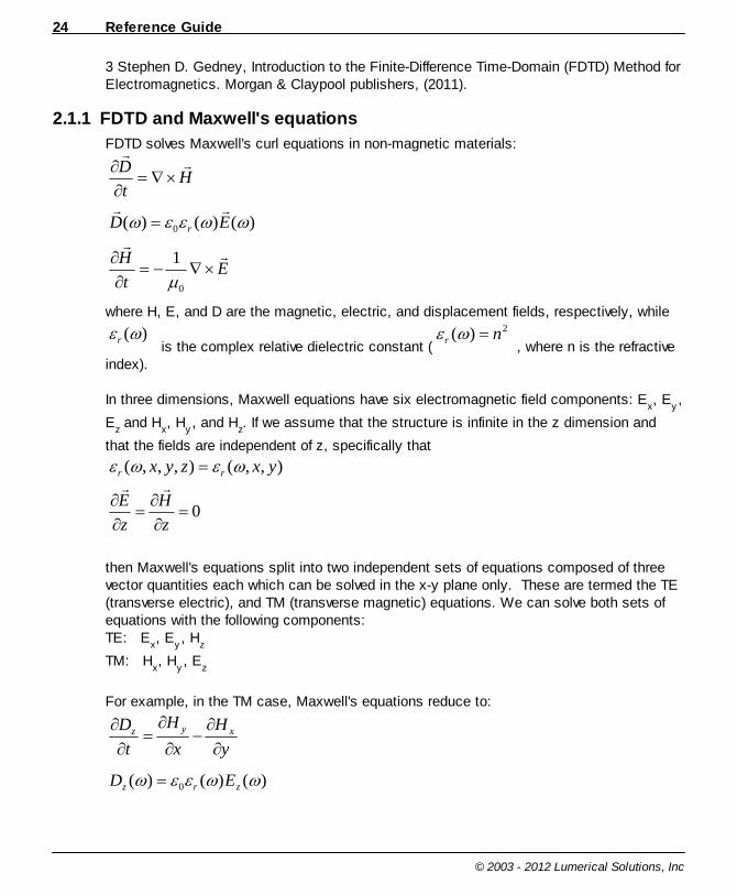
Reference Guide24
© 2003 - 2012 Lumerical Solutions, Inc
3 Stephen D. Gedney, Introduction to the Finite-Difference Time-Domain (FDTD) Method forElectromagnetics. Morgan & Claypool publishers, (2011).
2.1.1 FDTD and Maxwell's equations
FDTD solves Maxwell's curl equations in non-magnetic materials:
Ht
D
)()()( 0 ED r
Et
H
0
1
where H, E, and D are the magnetic, electric, and displacement fields, respectively, while
)(r is the complex relative dielectric constant (
2)( nr, where n is the refractive
index).
In three dimensions, Maxwell equations have six electromagnetic field components: Ex, E
y,
Ez and H
x, H
y, and H
z. If we assume that the structure is infinite in the z dimension and
that the fields are independent of z, specifically that
),,(),,,( yxzyx rr
0z
H
z
E
then Maxwell's equations split into two independent sets of equations composed of threevector quantities each which can be solved in the x-y plane only. These are termed the TE(transverse electric), and TM (transverse magnetic) equations. We can solve both sets ofequations with the following components:TE: E
x, E
y, H
z
TM: Hx, H
y, E
z
For example, in the TM case, Maxwell's equations reduce to:
y
H
x
H
t
D xyz
)()()( 0 zrz ED

Solver physics 25
© 2003 - 2012 Lumerical Solutions, Inc
y
E
t
H zx
0
1
x
E
t
Hzy
0
1
FDTD Solutions can solve the two and three dimensional Maxwell's equations in dispersivemedia and some simple non-linear media, where the user can specify arbitrary geometricstructures and various input excitation sources. The two dimensional FDTD simulatorsolves the TE and/or TM Maxwell equations.
FDTD is a time domain technique, meaning that the electromagnetic fields are solved as afunction of time. In general, FDTD Solutions is used to calculate the electromagnetic fieldsas a function of frequency or wavelength by performing Fourier transforms during thesimulation. This allows it to obtain complex-valued fields and other derived quantities suchas the complex Poynting vector, normalized transmission, and far field projections as afunction of frequency or wavelength. The field information can be returned in two differentnormalization states, please see the section on frequency domain normalization for moredetails.
Dispersive materials with tabulated refractive index (n,k) data as a function of wavelengthcan be solved using the multi-coefficient models with auto-fitting. Alternatively, specifictheoretical models such as Plasma (Drude), Debye or Lorentz can be used. See thechapter on the Material Database for details.
Boundary conditions are very important in electromagnetics and simulation techniques. FDTD Solutions/propagator supports a range of boundary conditions, such as PML,periodic, and Bloch. See the boundary conditions section here for the complete list.
Sources are another important component of a simulation. FDTD Solutions/propagatorsupports a number of different types of sources such as point dipoles, beams, plane waves,a total-field scattered-field (TFSF) source, a guided-mode source for integrated opticalcomponents, and an imported source to interface with external photonic design softwares. Detailed information about each of these sources is contained in the Radiation sourcessection.
Unless otherwise specified, all quantities in FDTD Solutions/propagator are calculated in SIunits. Please see Units and Normalization for more information.
The online User Guide at http://docs.lumerical.com/en/fdtd/knowledge_base.html has manymore details about the physics of FDTD and how to obtain advanced results. Please see,for example, the sections on coherence, and far field calculations in the online User Guide.
116
86
91

Reference Guide26
© 2003 - 2012 Lumerical Solutions, Inc
2.1.2 Meshing in FDTD
FDTD Solutions uses a rectangular, Cartesian style mesh, like the one shown in thefollowing screenshot. It's important to understand that of the fundamental simulationquantities (material properties and geometrical information, electric and magnetic fields) arecalculated at each mesh point. Obviously, using a smaller mesh allows for a moreaccurate representation of the device, but at a substantial cost. As the mesh becomessmaller, the simulation time and memory requirements will increase. FDTD Solutionsprovides a number of features, including the conformal mesh algorithm, that allow you toobtain accurate results, even when using a relatively coarse mesh.
By default, the simulation mesh is automatically generated.To maintain accuracy, the meshing algorithm will create asmaller mesh in high index (to maintain a constant numberof mesh points per wavelength) and highly absorbing(resolve penetration depths) materials. In some cases, it isalso necessary to manually add additional meshingconstraints. Usually, this involves forcing the mesh to besmaller near complex structures (often metal) where thefields are changing very rapidly.
2.2 Eigenmode SolverThe Eigenmode Solver (Eigensolver) solves for optical modes in a cross-section of anarbitrary waveguide geometry. The waveguide mode as a transverse field distribution thatpropagates along the waveguide without changing shape.
In the z-normal eigenmode solver simulation example shown in the figure above, we havethe vector fields:
)(),( ztieyxE and
)(),( ztieyxH
where ω is the angular frequency and β is the propagation constant. The modal effective
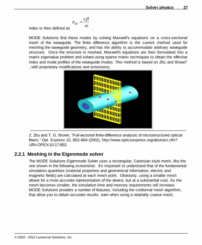
Solver physics 27
© 2003 - 2012 Lumerical Solutions, Inc
index is then defined as
cneff
.
MODE Solutions find these modes by solving Maxwell's equations on a cross-sectionalmesh of the waveguide. The finite difference algorithm is the current method used formeshing the waveguide geometry, and has the ability to accommodate arbitrary waveguidestructure. Once the structure is meshed, Maxwell's equations are then formulated into amatrix eigenvalue problem and solved using sparse matrix techniques to obtain the effective
index and mode profiles of the waveguide modes. This method is based on Zhu and Brown1
, with proprietary modifications and extensions.
Z. Zhu and T. G. Brown, “Full-vectorial finite-difference analysis of microstructured opticalfibers,” Opt. Express 10, 853–864 (2002), http://www.opticsexpress.org/abstract.cfm?URI=OPEX-10-17-853
2.2.1 Meshing in the Eigenmode solver
The MODE Solutions Eigenmode Solver uses a rectangular, Cartesian style mesh, like theone shown in the following screenshot. It's important to understand that of the fundamentalsimulation quantities (material properties and geometrical information, electric andmagnetic fields) are calculated at each mesh point. Obviously, using a smaller meshallows for a more accurate representation of the device, but at a substantial cost. As themesh becomes smaller, the simulation time and memory requirements will increase. MODE Solutions provides a number of features, including the conformal mesh algorithm,that allow you to obtain accurate results, even when using a relatively coarse mesh.
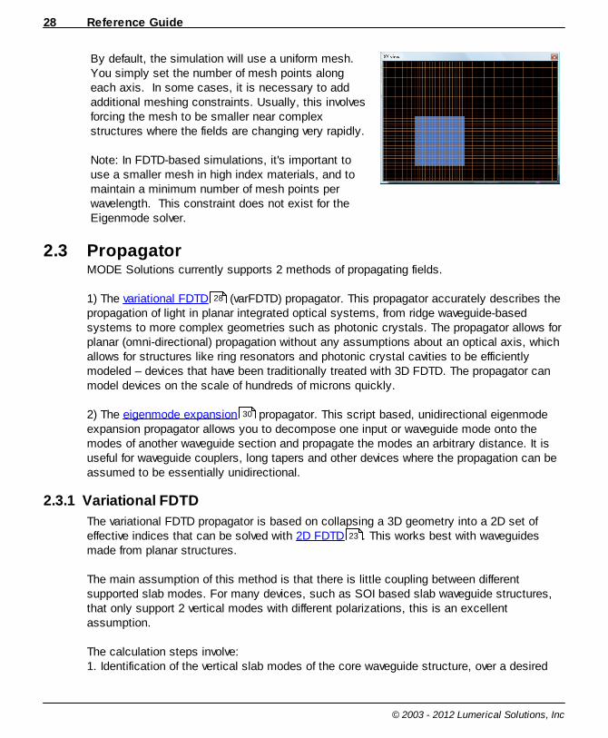
Reference Guide28
© 2003 - 2012 Lumerical Solutions, Inc
By default, the simulation will use a uniform mesh. You simply set the number of mesh points alongeach axis. In some cases, it is necessary to addadditional meshing constraints. Usually, this involvesforcing the mesh to be smaller near complexstructures where the fields are changing very rapidly.
Note: In FDTD-based simulations, it's important touse a smaller mesh in high index materials, and tomaintain a minimum number of mesh points perwavelength. This constraint does not exist for theEigenmode solver.
2.3 PropagatorMODE Solutions currently supports 2 methods of propagating fields.
1) The variational FDTD (varFDTD) propagator. This propagator accurately describes thepropagation of light in planar integrated optical systems, from ridge waveguide-basedsystems to more complex geometries such as photonic crystals. The propagator allows forplanar (omni-directional) propagation without any assumptions about an optical axis, whichallows for structures like ring resonators and photonic crystal cavities to be efficientlymodeled – devices that have been traditionally treated with 3D FDTD. The propagator canmodel devices on the scale of hundreds of microns quickly.
2) The eigenmode expansion propagator. This script based, unidirectional eigenmodeexpansion propagator allows you to decompose one input or waveguide mode onto themodes of another waveguide section and propagate the modes an arbitrary distance. It isuseful for waveguide couplers, long tapers and other devices where the propagation can beassumed to be essentially unidirectional.
2.3.1 Variational FDTD
The variational FDTD propagator is based on collapsing a 3D geometry into a 2D set ofeffective indices that can be solved with 2D FDTD . This works best with waveguidesmade from planar structures.
The main assumption of this method is that there is little coupling between differentsupported slab modes. For many devices, such as SOI based slab waveguide structures,that only support 2 vertical modes with different polarizations, this is an excellentassumption.
The calculation steps involve:1. Identification of the vertical slab modes of the core waveguide structure, over a desired
28
30
23
Solver physics 29
© 2003 - 2012 Lumerical Solutions, Inc
range of wavelengths. 2. Meshing of the structure and collapse of the 3rd dimension by calculation of the
corresponding effective 2D indices (taking into account the vertical slab mode profile).There are currently two approaches to doing this in the Propagator:
VariationalA variational procedure based on Hammer and Ivanova1. Here, the effective permittivities ofthe TE and TM-like modes have the form:
z
z
r
rTEeff
dzzM
dzzMzzyx
kyx
2
2
2
),(
),(),(),,(
),,(
z
z r
z
z rrTMeff
dzMzyx
k
dzz
M
zyx
dzMzyx
dzM
kyx
22
2
2
22
),,(
1
),,(
11
||),,(
1
||1
),,(
where εr, M and βr are the 1-D reference permittivity profile, the associated guided slabmode and the propagation constant.
Reciprocity BasedThis is a procedure based on the reciprocity theorem, as described in Snyder and Love2:
z
z
r
reff
dznP
dzzEzzyx
kyxn
2
2
1
0
0
),(),(),,(
),,(
Note that in both cases, the generated effective materials are also dispersive, where thedispersion comes both from the original material properties (material dispersion) and theslab waveguide geometry (waveguide dispersion). These new materials are then fitted usingLumerical Solutions' multi-coefficient model into a time-domain form that can be used in the2D FDTD simulation in step 3. Note that the effective index treatment may lead togenerated materials that have properties that are unphysical (for example, having anartificial negative imaginary index). In this case, one has the option of restricting the rangeof generated indices to the min/max values defined by the physical material properties ofthe original materials. All of these settings can be found under the Effective index tab of thePropagator simulation region.
3. Simulation of the structure in 2D by FDTD .4. If desired, re-expansion of the fields into 3D.
23
Reference Guide30
© 2003 - 2012 Lumerical Solutions, Inc
The Ring resonator getting started example contains step-by-step instructions anddiscussions on how to carry out a propagator simulation using the variational FDTDmethod.
1 Manfred Hammer and Olena V. Ivanova, MESA Institute for Nanotechnology, University ofTwente, Enschede, The Netherlands"Effective index approximation of photonic crystal slabs: a 2-to-1-D assessment", Opticaland Quantum Electronics ,Volume 41, Number 4, 267-283, DOI: 10.1007/s11082-009-9349-32 Allan W. Snyder and John D. Love, Optical Waveguide Theory. Chapman & Hall, London,England, 1983.
2.3.2 Eigenmode expansion
This unidirectional eigenmode expansion method is implemented in the propagatecommand.
The propagate command calculates the resulting mode profile of an arbitrary mode after ithas propagated through a waveguide for some distance. This is done by decomposing themode into modes supported by the waveguide (ie. the currently calculated modes) using overlap integrals . Each supported mode is then propagated through the waveguide.The resulting modes are then added coherently to give the final mode profile.
This technical is useful for waveguide couplers, long tapers and other devices where thepropagation can be assumed to be essentially uni-directional. Please see MODE Solutions'applications library for some use case examples:Evanescent waveguide couplersTapered waveguidesPolarization rotator
2.3.3 Meshing in the propagator
The MODE Solutions Propagator uses a rectangular, Cartesian style mesh, like the oneshown in the following screenshot. It's important to understand that of the fundamentalsimulation quantities (material properties and geometrical information, electric andmagnetic fields) are calculated at each mesh point. Obviously, using a smaller meshallows for a more accurate representation of the device, but at a substantial cost. As themesh becomes smaller, the simulation time and memory requirements will increase. MODE Solutions provides a number of features, including the conformal mesh algorithm,that allow you to obtain accurate results, even when using a relatively coarse mesh.
341
339

Solver physics 31
© 2003 - 2012 Lumerical Solutions, Inc
By default, the simulation mesh is automaticallygenerated. To maintain accuracy, the meshingalgorithm will create a smaller mesh in high index (tomaintain a constant number of mesh points perwavelength) and highly absorbing (resolve penetrationdepths) materials. In some cases, it is alsonecessary to manually add additional meshingconstraints. Usually, this involves forcing the mesh tobe smaller near complex structures (often metal)where the fields are changing very rapidly.
Note: meshing timeThe general meshing algorithm can take a reasonable amount of time compared to thesimulation because the mesh must be effectively completed in 3D. It is possible for theuser to specify if the structure is composed of purely extruded structures - that isstructures that are extruded along z with perfectly vertical sidewalls. In this case, themeshing can be accomplished much faster.
2.4 INTERCONNECTINTERCONNECT is a circuit simulator that can support mixed signal representation ofoptical single and multi-mode signals as well as electrical signals. The signals canpropagate fully bidirectionally through the circuit topology for both Time Domain andFrequency Domain simulations.
Users can choose elements from an extensive list of pre-defined PIC elements, as well ascreate custom elements from pre-defined primitives or via Lumerical’s powerful scriptlanguage. In addition, elements can also be characterized accurately using results directlyfrom Lumerical's electromagnetic simulators (FDTD Solutions and MODE Solutions).
2.4.1 Time Domain Simulator
Time domain simulation is performed using a data flow system simulator, allowing for moreflexibility than using traditional discrete time or time-driven simulators. The simulatorscheduler calculates each element in order to generate time domain waveform samples andpropagate them bidirectionally. Very close coupling between components can be simulatedallowing, for example, the analysis of optical resonators.
31
32
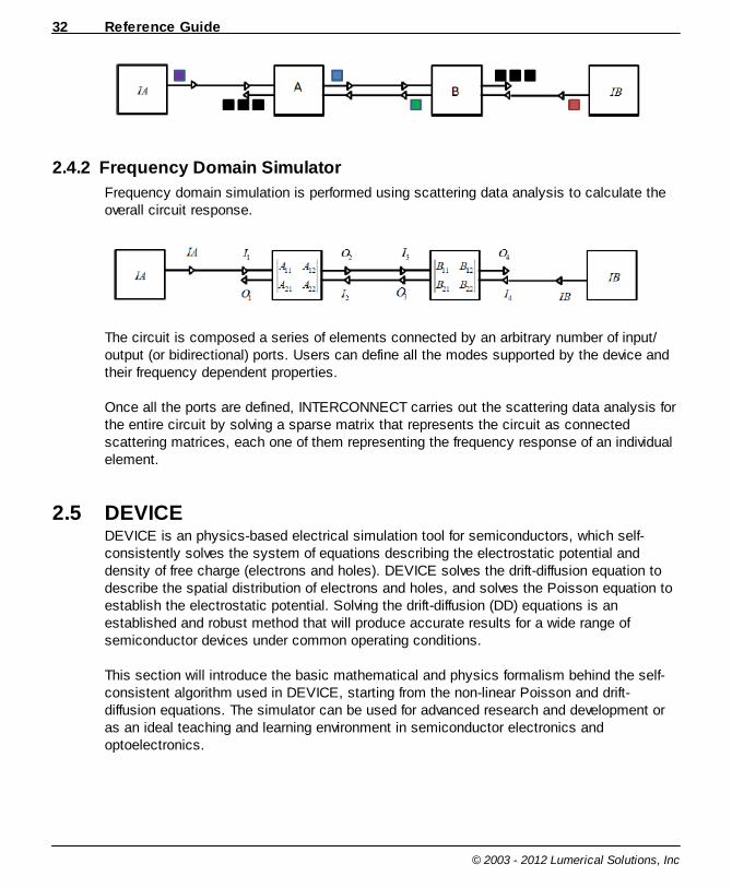
Reference Guide32
© 2003 - 2012 Lumerical Solutions, Inc
2.4.2 Frequency Domain Simulator
Frequency domain simulation is performed using scattering data analysis to calculate theoverall circuit response.
The circuit is composed a series of elements connected by an arbitrary number of input/output (or bidirectional) ports. Users can define all the modes supported by the device andtheir frequency dependent properties.
Once all the ports are defined, INTERCONNECT carries out the scattering data analysis forthe entire circuit by solving a sparse matrix that represents the circuit as connectedscattering matrices, each one of them representing the frequency response of an individualelement.
2.5 DEVICEDEVICE is an physics-based electrical simulation tool for semiconductors, which self-consistently solves the system of equations describing the electrostatic potential anddensity of free charge (electrons and holes). DEVICE solves the drift-diffusion equation todescribe the spatial distribution of electrons and holes, and solves the Poisson equation toestablish the electrostatic potential. Solving the drift-diffusion (DD) equations is anestablished and robust method that will produce accurate results for a wide range ofsemiconductor devices under common operating conditions.
This section will introduce the basic mathematical and physics formalism behind the self-consistent algorithm used in DEVICE, starting from the non-linear Poisson and drift-diffusion equations. The simulator can be used for advanced research and development oras an ideal teaching and learning environment in semiconductor electronics andoptoelectronics.
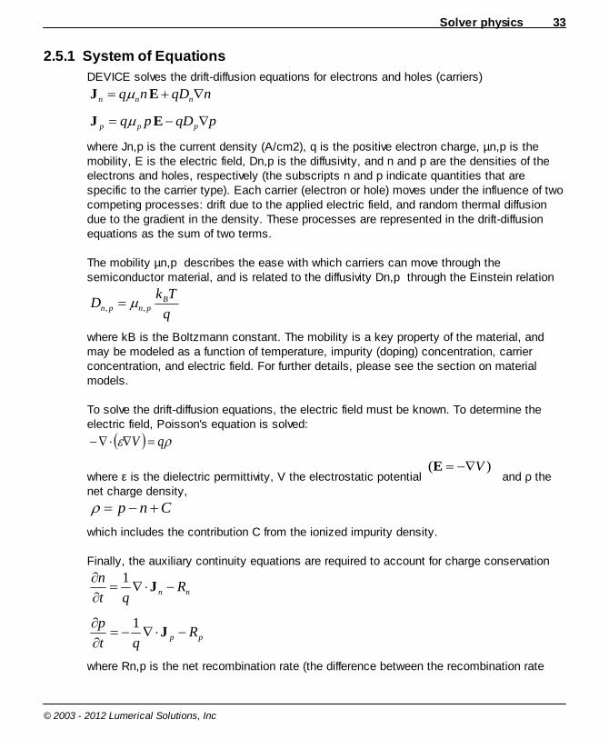
Solver physics 33
© 2003 - 2012 Lumerical Solutions, Inc
2.5.1 System of Equations
DEVICE solves the drift-diffusion equations for electrons and holes (carriers)
nqDnq nnn EJ
pqDpq ppp EJ
where Jn,p is the current density (A/cm2), q is the positive electron charge, µ n,p is themobility, E is the electric field, Dn,p is the diffusivity, and n and p are the densities of theelectrons and holes, respectively (the subscripts n and p indicate quantities that arespecific to the carrier type). Each carrier (electron or hole) moves under the influence of twocompeting processes: drift due to the applied electric field, and random thermal diffusiondue to the gradient in the density. These processes are represented in the drift-diffusionequations as the sum of two terms.
The mobility µ n,p describes the ease with which carriers can move through thesemiconductor material, and is related to the diffusivity Dn,p through the Einstein relation
q
TkD B
pnpn ,,
where kB is the Boltzmann constant. The mobility is a key property of the material, andmay be modeled as a function of temperature, impurity (doping) concentration, carrierconcentration, and electric field. For further details, please see the section on materialmodels.
To solve the drift-diffusion equations, the electric field must be known. To determine theelectric field, Poisson's equation is solved:
qV
where ε is the dielectric permittivity, V the electrostatic potential )( VE
and ρ thenet charge density,
Cnp
which includes the contribution C from the ionized impurity density.
Finally, the auxiliary continuity equations are required to account for charge conservation
nn Rqt
nJ
1
pp Rqt
pJ
1
where Rn,p is the net recombination rate (the difference between the recombination rate

Reference Guide34
© 2003 - 2012 Lumerical Solutions, Inc
and generation rate). The physical processes associated with the material are assumed toact equivalently when applied to electrons or holes, and as a result, R = Rn = Rp. Therecombination and generation processes are important factors in the material-specificcalculation of carrier behavior. Multiple recombination and generation processes aremodeled, which may depend on temperature, impurity (doping) concentration, carrierconcentration, electric field, and current density. For further details, please see the sectionon material models.
DEVICE discretizes and solves the drift-diffusion and Poisson’s equations on anunstructured finite-element mesh in one and two dimensions. The simulation region ispartitioned into multiple domains along boundaries between materials with unique physicaldescriptions. The materials used in the simulation may be categorized as insulators,semiconductors, or conductors; each type of material has an associated user-specifiedmodel or collection of models that describe its behavior. In particular, specialized multi-coefficient models are provided for semiconductors that describe the fundamentalproperties, mobility, and recombination processes inherent to that material.
The system of equations solved by DEVICE admits both a steady-state and time-varyingresult. By enforcing the condition
0t
p
t
n
in the continuity equations, the carrier density and electrostatic potential can be solved atsteady-state. Steady-state simulations can be used to examine the system’s behavior at afixed operating point, and are also useful when extracting small-signal parameters for acomponent (e.g. for frequency response analysis). Alternately, by specifying an initialcondition for the carrier density and electrostatic potential, the equations can be solved in asequence of discrete times. The time-dependent behavior of the component can then beused to directly evaluate its large-signal time-domain response or extract large-signal ACparameters.
Boundary conditions are very important in an accurate semiconductor device simulation.Two categories of boundary condition are present in DEVICE: those that relate to theelectrostatic potential (Poisson’s equation) and those that relate to the carrier densities(the drift-diffusion equations). Poisson’s equation and the drift-diffusion equations aresecond-order partial differential equations (PDE), and each requires that the solution beexplicitly specified for at least one location. This is known as a Dirichlet boundarycondition. For the electrostatic potential, the Dirichlet condition takes the form of aboundary (internal or external) with a fixed voltage specified,
1)( VxV
as is typical of an electrical contact. For the carrier densities, the majority carrierconcentration is set to its equilibrium value at the interface between a contact and the
Solver physics 35
© 2003 - 2012 Lumerical Solutions, Inc
semiconductor, such that
0Cnp
At internal boundaries between two domains that are not contacts, the boundary conditionsare determined from the physical properties of the interface. In the case of the electrostaticpotential, the electric flux density must be continuous across the boundary in the absenceof a surface charge. For the electron and hole densities, boundary conditions between thesemiconductor and adjacent materials may be specified in terms of a surfacerecombination current density, which will default to zero (no carrier flux across theboundary) for insulators or an infinite recombination velocity (forcing the carrier density toits equilibrium value) for contacts. At the external (open) boundaries of the simulationdomain, homogenous Neumann boundary conditions are applied: the electric field normal tothe boundary is set to zero as is the surface recombination current density. Physically, thiscorresponds to an insulating boundary across which no charge can flow.
By convention, the length units in semiconductor models are chosen to be centimeters.This is reflected in the semiconductor device literature, and in the parameter coefficients forthe material models. Energies are calculated in electron Volts (eV), where the electronenergy E is related to the local electrostatic potential (voltage) as E = -qV. All energies(and voltages) are referenced from the (equilibrium) Fermi level of an electrical contact inthe system.
2.5.2 Meshing in DEVICE
DEVICE uses an unstructured, finite-element mesh, like the one shown in the followingscreenshot. The solution to the system of equations used to determine the physicalquantities of interest is estimated from the discrete formulation of those equations.Consequently, it's important to understand that of the fundamental simulation quantities(material properties, geometry information, electrostatic potential, and carrierconcentrations) are calculated at each mesh vertex.

Reference Guide36
© 2003 - 2012 Lumerical Solutions, Inc
A finer mesh (with shorter edge lengths and smallerelements) will better approximate the exact solutionto the system of equations, but at a substantial cost.As the mesh features become smaller, the simulationtime and memory requirements will increase. DEVICE provides a number of tools, including theautomatic and guided mesh refinement, that allowyou to obtain accurate results, while minimizingcomputational effort.
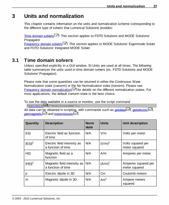
Units and normalization 37
© 2003 - 2012 Lumerical Solutions, Inc
3 Units and normalization
This chapter contains information on the units and normalization scheme corresponding tothe different type of solvers that Lumerical Solutions provides:
Time domain solvers : This section applies to FDTD Solutions and MODE Solutions'PropagatorFrequency domain solvers : This section applies to MODE Solutions' Eigenmode Solverand FDTD Solutions' Integrated MODE Solver
3.1 Time domain solversUnless specified explicitly in a GUI window, SI Units are used at all times. The followingtable summarizes the units used in time domain solvers (ex. FDTD Solutions and MODESolutions' Propagator).
Please note that some quantities can be returned in either the Continuous WaveNormalization state (cwnorm) or the No Normalization state (nonorm). Please see Frequency domain normalization for details on the different normalization states. Formost applications, the default cwnorm state is the best choice.
To see the data available in a source or monitor, use the script command?getdata ("monitorname");
All data can be obtained in scripting, with commands such as getdata , getelectric ,getmagnetic and transmission .
Quantity Description Normstate
Units Unit description
E(t) Electric field as functionof time
N/A V/m Volts per meter
|E(t)|2 Electric field intensity asa function of time
N/A (V/m)2 Volts squared permeter squared
H(t) Magnetic field as afunction
N/A A/m Amperes per meter
|H(t)|2 Magnetic field intensity asa function of time
N/A (A/m)2 Amperes squared permeter squared
p Electric dipole in 3D N/A Cm Coulomb meters
m Magnetic dipole in 3D N/A Am2 Ampere meterssquared
37
48
39
349
349 353
354 321
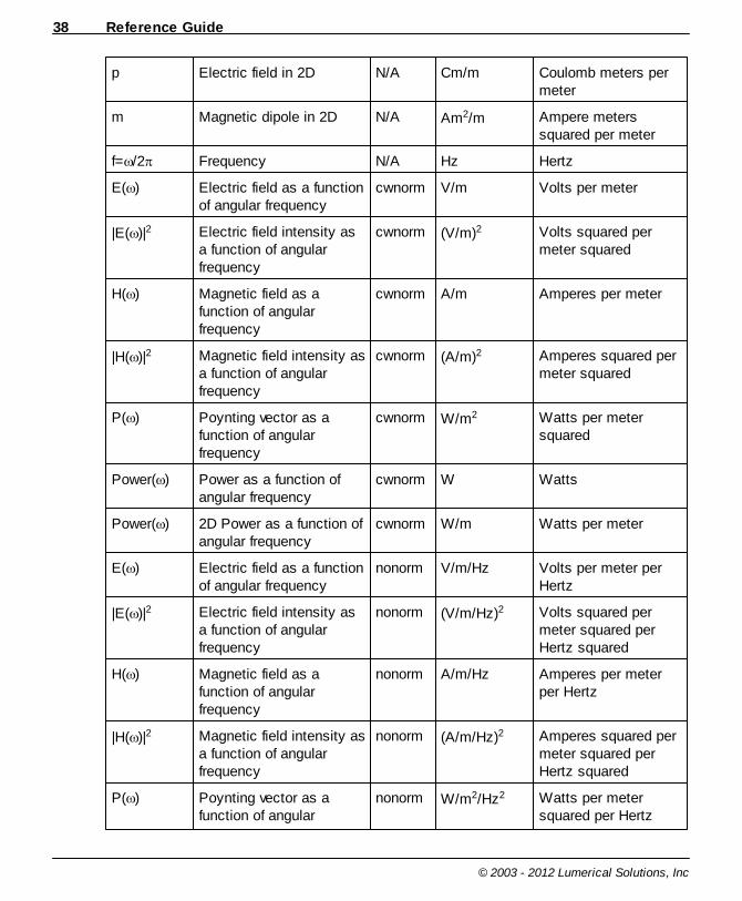
Reference Guide38
© 2003 - 2012 Lumerical Solutions, Inc
p Electric field in 2D N/A Cm/m Coulomb meters permeter
m Magnetic dipole in 2D N/A Am2/m Ampere meterssquared per meter
f= /2 Frequency N/A Hz Hertz
E( ) Electric field as a functionof angular frequency
cwnorm V/m Volts per meter
|E( )|2 Electric field intensity asa function of angularfrequency
cwnorm (V/m)2 Volts squared permeter squared
H( ) Magnetic field as afunction of angularfrequency
cwnorm A/m Amperes per meter
|H( )|2 Magnetic field intensity asa function of angularfrequency
cwnorm (A/m)2 Amperes squared permeter squared
P( ) Poynting vector as afunction of angularfrequency
cwnorm W/m2 Watts per metersquared
Power( ) Power as a function ofangular frequency
cwnorm W Watts
Power( ) 2D Power as a function ofangular frequency
cwnorm W/m Watts per meter
E( ) Electric field as a functionof angular frequency
nonorm V/m/Hz Volts per meter perHertz
|E( )|2 Electric field intensity asa function of angularfrequency
nonorm (V/m/Hz)2 Volts squared permeter squared perHertz squared
H( ) Magnetic field as afunction of angularfrequency
nonorm A/m/Hz Amperes per meterper Hertz
|H( )|2 Magnetic field intensity asa function of angularfrequency
nonorm (A/m/Hz)2 Amperes squared permeter squared perHertz squared
P( ) Poynting vector as afunction of angular
nonorm W/m2/Hz2 Watts per metersquared per Hertz
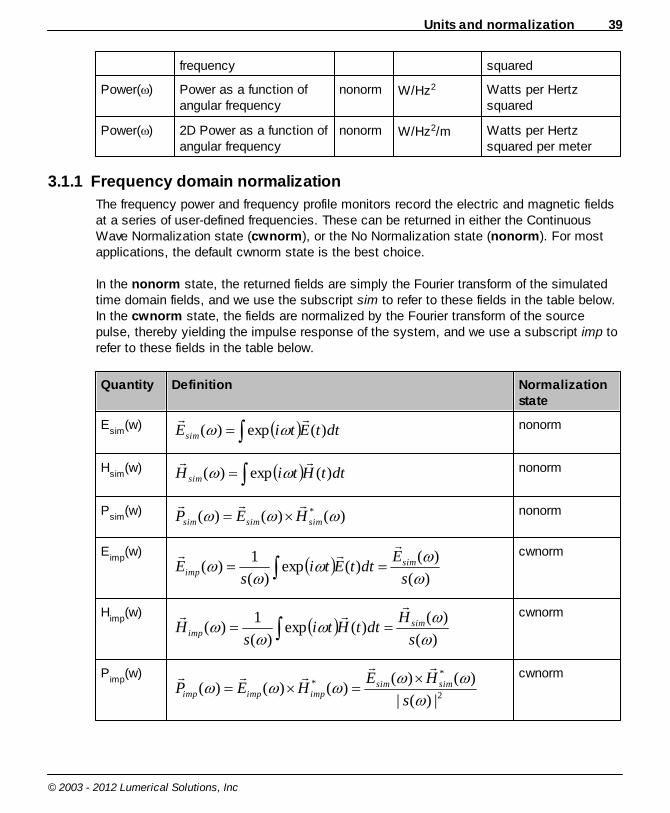
Units and normalization 39
© 2003 - 2012 Lumerical Solutions, Inc
frequency squared
Power( ) Power as a function ofangular frequency
nonorm W/Hz2 Watts per Hertzsquared
Power( ) 2D Power as a function ofangular frequency
nonorm W/Hz2/m Watts per Hertzsquared per meter
3.1.1 Frequency domain normalization
The frequency power and frequency profile monitors record the electric and magnetic fieldsat a series of user-defined frequencies. These can be returned in either the ContinuousWave Normalization state (cwnorm), or the No Normalization state (nonorm). For mostapplications, the default cwnorm state is the best choice.
In the nonorm state, the returned fields are simply the Fourier transform of the simulatedtime domain fields, and we use the subscript sim to refer to these fields in the table below.In the cwnorm state, the fields are normalized by the Fourier transform of the sourcepulse, thereby yielding the impulse response of the system, and we use a subscript imp torefer to these fields in the table below.
Quantity Definition Normalizationstate
Esim
(w) dttEtiEsim )(exp)( nonorm
Hsim
(w) dttHtiH sim )(exp)( nonorm
Psim
(w) )()()( *simsimsim HEP nonorm
Eimp
(w)
)(
)()(exp
)(
1)(
s
EdttEti
sE sim
imp
cwnorm
Himp
(w)
)(
)()(exp
)(
1)(
s
HdttHti
sH sim
imp
cwnorm
Pimp
(w)
2
**
|)(|
)()()()()(
s
HEHEP simsim
impimpimp
cwnorm
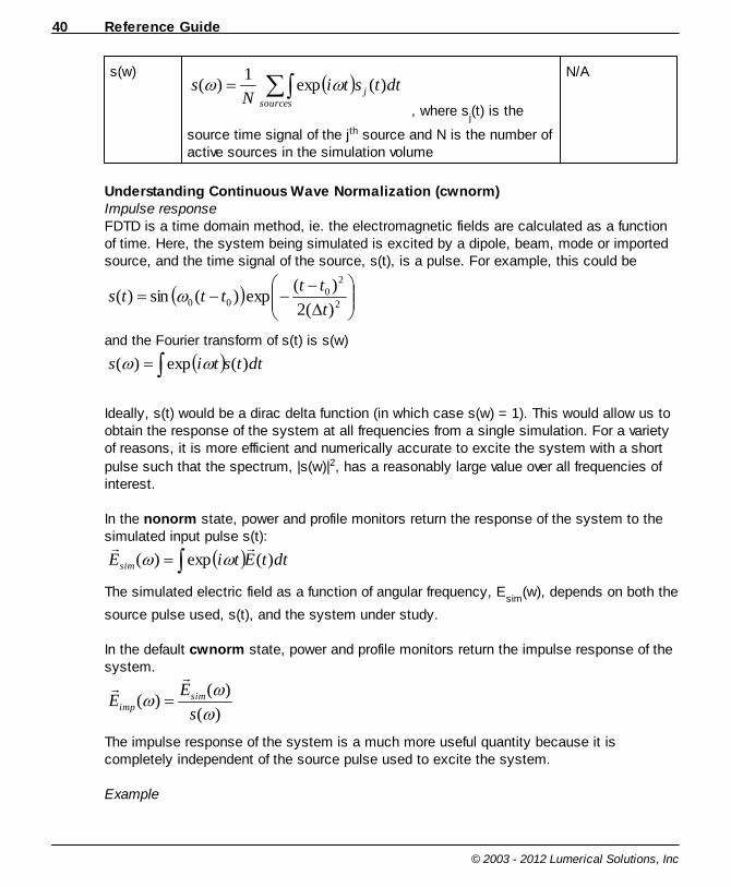
Reference Guide40
© 2003 - 2012 Lumerical Solutions, Inc
s(w)
sourcesj dttsti
Ns )(exp
1)(
, where sj(t) is the
source time signal of the jth source and N is the number ofactive sources in the simulation volume
N/A
Understanding Continuous Wave Normalization (cwnorm)Impulse responseFDTD is a time domain method, ie. the electromagnetic fields are calculated as a functionof time. Here, the system being simulated is excited by a dipole, beam, mode or importedsource, and the time signal of the source, s(t), is a pulse. For example, this could be
2
20
00)(2
)(exp)(sin)(
t
ttttts
and the Fourier transform of s(t) is s(w)
dttstis )(exp)(
Ideally, s(t) would be a dirac delta function (in which case s(w) = 1). This would allow us toobtain the response of the system at all frequencies from a single simulation. For a varietyof reasons, it is more efficient and numerically accurate to excite the system with a short
pulse such that the spectrum, |s(w)|2, has a reasonably large value over all frequencies ofinterest.
In the nonorm state, power and profile monitors return the response of the system to thesimulated input pulse s(t):
dttEtiEsim )(exp)(
The simulated electric field as a function of angular frequency, Esim
(w), depends on both the
source pulse used, s(t), and the system under study.
In the default cwnorm state, power and profile monitors return the impulse response of thesystem.
)(
)()(
s
EE sim
imp
The impulse response of the system is a much more useful quantity because it iscompletely independent of the source pulse used to excite the system.
Example

Units and normalization 41
© 2003 - 2012 Lumerical Solutions, Inc
Consider a beam source injected into free space at z=z0. The source signal is
2
20
00)(2
)(exp)(sin)(
t
ttttts
The electric field at the source injection plane has the following form:
)(),,(),,,( 000 tszyxEtzyxE
In the cwnorm state,
),,(),,,( 0 zyxEzyxE
In other words, the field returned in the cwnorm state is the field that would exist if a CWsource of amplitude E
0 had been used at the angular frequency . It removes any frequency
dependence due to the finite pulse length of the source, and the units of the returned fieldsare the same as time domain fields.
3.1.2 Spectral averaging
For some simulations, it is useful to calculate the incoherent spectral average of theelectromagnetic fields or the Poynting vector. For example, we might want to calculate
dPWP imp )()(
where W( ) is a weighting function and Pimp
( ) is the Poynting vector returned in the
cwnorm state, in other words, the impulse response of the system. (Please seeFrequency domain normalization for an explanation of the impulse response.) We couldcalculate the P
imp( ) at many different angular frequencies and then perform the spectral
average after the simulation. FDTD Solutions, however, allows for two methods of moreefficient spectral averaging during the simulation which can significantly reduce the memoryrequirements and increase the speed of the simulation. These methods are called "totalspectral averaging" and "partial spectral averaging".
The frequency power and frequency profile monitors can record spectral averages of variousquantities during the simulation. Like the other quantities calculated by these monitors,these can be returned in the Continuous Wave Normalization state (cwnorm), or the NoNormalization state (nonorm). For most applications, the default cwnorm state is the bestchoice. In the tables below, we use the subscripts sim and imp to refer to the quantitiesreturned in the nonorm and cwnorm states respectively. Please refer to Frequency domainnormalization for more details on the two normalization states, and obtaining theimpulse response of the system.
Total spectral averagingFDTD Solutions/Propagator supports a spectral average that uses the source input
39
39

Reference Guide42
© 2003 - 2012 Lumerical Solutions, Inc
spectrum as the weighting function. Total spectral averaging can be useful when the sourcespectrum of the simulation matches the actual illumination conditions. The following tablegives the precise definitions of the quantities available using total spectral averaging.
Quantity Definition Normalizationstate
<|Esim
|2>total
0
22
)( dEE simtotal
sim
nonorm
<|Hsim
|2>total
0
22
)( dHH simtotal
sim
nonorm
<Psim
>total
0
)( dPP simtotal
sim
nonorm
<|Eimp
|2>total
0
2
0
22
2
)(
)()(
ds
dEs
Eimp
totalimp
cwnorm
<|Himp
|2>total
0
2
0
22
2
)(
)()(
ds
dHs
Himp
totalimp
cwnorm
<Pimp
>total
0
2
0
2
)(
)()(
ds
dPs
Pimp
totalimp
cwnorm

Units and normalization 43
© 2003 - 2012 Lumerical Solutions, Inc
s(w)
sourcesj dttsti
Ns )(exp
1)(
, where sj(t) is the
source time signal of the jth source and N is the numberof active sources in the simulation volume
N/A
Total spectral averaging can be turned on by selecting total spectral average as shown inthe screenshot below.
To see the data available in a monitor, use the script command?getdata ("monitorname");
All data can be obtained in scripting, with commands such as getdata andtransmission_avg . The available components for total spectral averaging are shown inthe following table.
Quantity Data name Example script command
<|Exsim
|2>total
E2x_avg nonorm;E2x = getdata("monitor1","E2x_avg");
<|Eysim
|2>total
E2y_avg nonorm;E2y = getdata("monitor1","E2y_avg");
<|Ezsim
|2>total
E2z_avg nonorm;E2z = getdata("monitor1","E2z_avg");
<|Hxsim
|2>total
H2x_avg nonorm;H2x = getdata("monitor1","H2x_avg");
<|Hysim
)|2>total
H2y_avg nonorm;H2y = getdata("monitor1","H2y_avg");
<|Hzsim
)|2>total
H2z_avg nonorm;H2z = getdata("monitor1","H2z_avg");
349
349
322
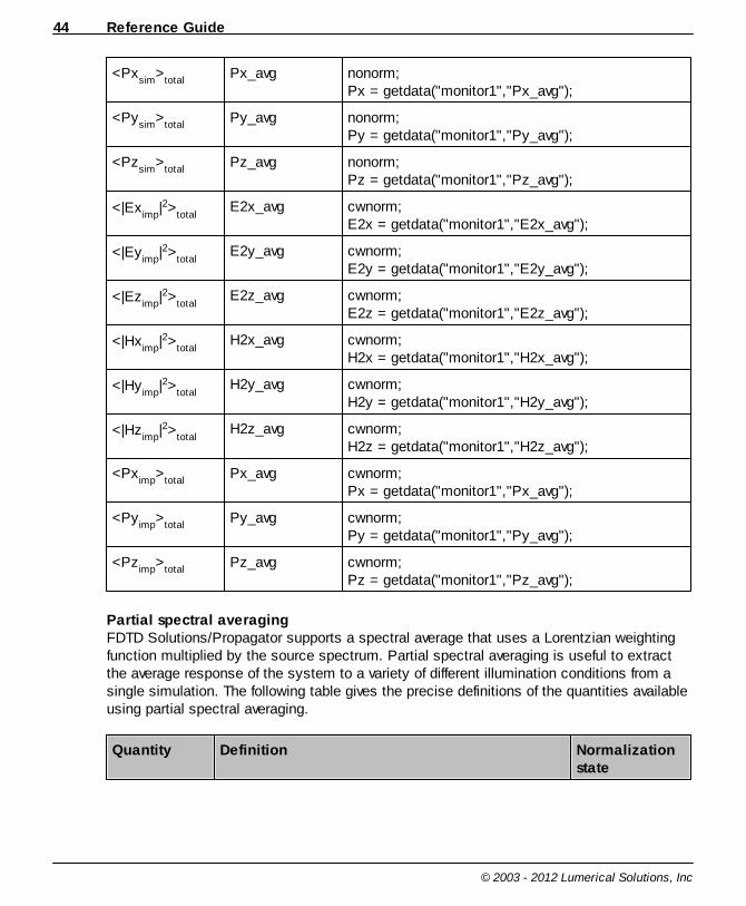
Reference Guide44
© 2003 - 2012 Lumerical Solutions, Inc
<Pxsim
>total
Px_avg nonorm;Px = getdata("monitor1","Px_avg");
<Pysim
>total
Py_avg nonorm;Py = getdata("monitor1","Py_avg");
<Pzsim
>total
Pz_avg nonorm;Pz = getdata("monitor1","Pz_avg");
<|Eximp
|2>total
E2x_avg cwnorm;E2x = getdata("monitor1","E2x_avg");
<|Eyimp
|2>total
E2y_avg cwnorm;E2y = getdata("monitor1","E2y_avg");
<|Ezimp
|2>total
E2z_avg cwnorm;E2z = getdata("monitor1","E2z_avg");
<|Hximp
|2>total
H2x_avg cwnorm;H2x = getdata("monitor1","H2x_avg");
<|Hyimp
|2>total
H2y_avg cwnorm;H2y = getdata("monitor1","H2y_avg");
<|Hzimp
|2>total
H2z_avg cwnorm;H2z = getdata("monitor1","H2z_avg");
<Pximp
>total
Px_avg cwnorm;Px = getdata("monitor1","Px_avg");
<Pyimp
>total
Py_avg cwnorm;Py = getdata("monitor1","Py_avg");
<Pzimp
>total
Pz_avg cwnorm;Pz = getdata("monitor1","Pz_avg");
Partial spectral averagingFDTD Solutions/Propagator supports a spectral average that uses a Lorentzian weightingfunction multiplied by the source spectrum. Partial spectral averaging is useful to extractthe average response of the system to a variety of different illumination conditions from asingle simulation. The following table gives the precise definitions of the quantities availableusing partial spectral averaging.
Quantity Definition Normalizationstate
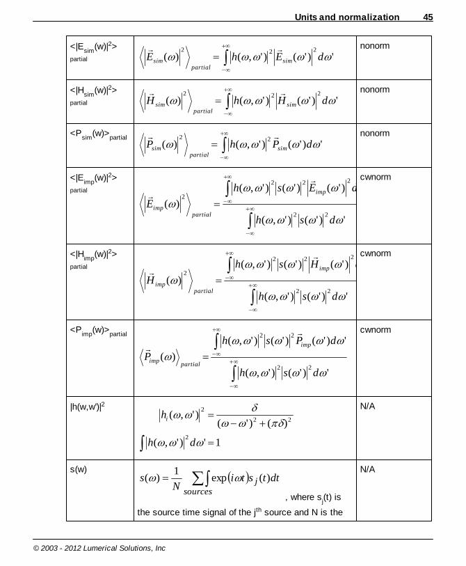
Units and normalization 45
© 2003 - 2012 Lumerical Solutions, Inc
<|Esim
(w)|2>
partial ')'()',()(222
dEhE simpartial
sim
nonorm
<|Hsim
(w)|2>
partial ')'()',()(222
dHhH simpartial
sim
nonorm
<Psim
(w)>partial
')'()',()(22
dPhP simpartial
sim
nonorm
<|Eimp
(w)|2>
partial
')'()',(
')'()'()',(
)(22
222
2
dsh
dEsh
Eimp
partialimp
cwnorm
<|Himp
(w)|2>
partial
')'()',(
')'()'()',(
)(22
222
2
dsh
dHsh
Himp
partialimp
cwnorm
<Pimp
(w)>partial
')'()',(
')'()'()',(
)(22
22
dsh
dPsh
Pimp
partialimp
cwnorm
|h(w,w')|2
1')',(
)()'()',(
2
22
2
dh
hi
N/A
s(w)
sourcesj dttsti
Ns )(exp
1)(
, where sj(t) is
the source time signal of the jth source and N is the
N/A
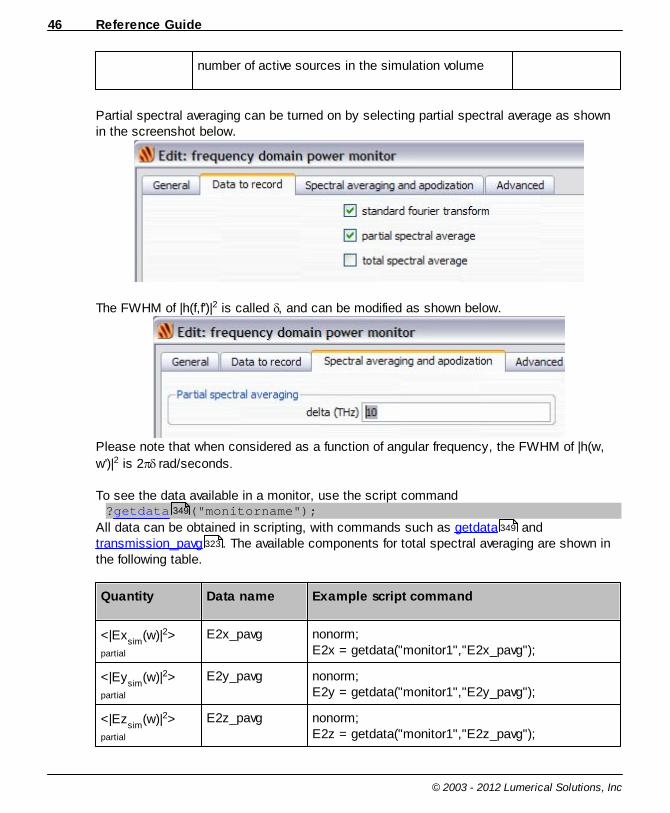
Reference Guide46
© 2003 - 2012 Lumerical Solutions, Inc
number of active sources in the simulation volume
Partial spectral averaging can be turned on by selecting partial spectral average as shownin the screenshot below.
The FWHM of |h(f,f')|2 is called , and can be modified as shown below.
Please note that when considered as a function of angular frequency, the FWHM of |h(w,
w')|2 is 2 rad/seconds
To see the data available in a monitor, use the script command?getdata ("monitorname");
All data can be obtained in scripting, with commands such as getdata andtransmission_pavg . The available components for total spectral averaging are shown inthe following table.
Quantity Data name Example script command
<|Exsim
(w)|2>
partial
E2x_pavg nonorm;E2x = getdata("monitor1","E2x_pavg");
<|Eysim
(w)|2>
partial
E2y_pavg nonorm;E2y = getdata("monitor1","E2y_pavg");
<|Ezsim
(w)|2>
partial
E2z_pavg nonorm;E2z = getdata("monitor1","E2z_pavg");
349
349
323

Units and normalization 47
© 2003 - 2012 Lumerical Solutions, Inc
<|Hxsim
(w)|2>
partial
H2x_pavg nonorm;H2x = getdata("monitor1","H2x_pavg");
<|Hysim
(w)|2>
partial
H2y_pavg nonorm;H2y = getdata("monitor1","H2y_pavg");
<|Hzsim
(w)|2>
partial
H2z_pavg nonorm;H2z = getdata("monitor1","H2z_pavg");
<Pxsim
(w)>partial
Px_pavg nonorm;Px = getdata("monitor1","Px_pavg");
<Pysim
(w)>partial
Py_pavg nonorm;Py = getdata("monitor1","Py_pavg");
<Pzsim
(w)>partial
Pz_pavg nonorm;Pz = getdata("monitor1","Pz_pavg");
<|Eximp
(w)|2>
partial
E2x_pavg cwnorm;E2x = getdata("monitor1","E2x_pavg");
<|Eyimp
(w)|2>
partial
E2y_pavg cwnorm;E2y = getdata("monitor1","E2y_pavg");
<|Ezimp
(w)|2>
partial
E2z_pavg cwnorm;E2z = getdata("monitor1","E2z_pavg");
<|Hximp
(w)|2>
partial
H2x_pavg cwnorm;H2x = getdata("monitor1","H2x_pavg");
<|Hyimp
(w)|2>
partial
H2y_pavg cwnorm;H2y = getdata("monitor1","H2y_pavg");
<|Hzimp
(w)|2>
partial
H2z_pavg cwnorm;H2z = getdata("monitor1","H2z_pavg");
<Pximp
(w)>partial
Px_pavg cwnorm;Px = getdata("monitor1","Px_pavg");
<Pyimp
(w)>partial
Py_pavg cwnorm;Py = getdata("monitor1","Py_pavg");
<Pzimp
(w)>partial
Pz_pavg cwnorm;Pz = getdata("monitor1","Pz_pavg");
Reference Guide48
© 2003 - 2012 Lumerical Solutions, Inc
3.1.3 Source amplitudes
Dipole sourcesFor dipole sources, amplitude refers to the amplitude of the point source whose units arelisted below. Base amplitude refers to the amplitude that will generate a radiated CW powerof 10 nW/m in 2D simulations and 1 fW in 3D simulations, and total amplitude refers to theamplitude actually used in the simulations which is the product of the amplitude and thebase amplitude.
Dipole source amplitudes areCm for 3D electric dipole sources
Am2 for 3D magnetic dipole sourcesCm/m for 2D electric dipole sources
Am2/m for 2D magnetic dipole sources
Other sourcesWhen specifying the amplitude for non-dipole sources, the "amplitude" refers to the peakelectric field amplitude in units of V/m. For example, if a Gaussian beam has the followingelectric field distribution in time and space:
20
22
2
20
000
)(exp
)(2
)(exp)(sin),,,(
w
yx
t
ttttEtzyxE
Then the "amplitude" refers to the value of E0 and has units of V/m.
3.2 Frequency domain solversUnless specified explicitly in a GUI window, SI Units are used at all times. Unlike timedomain solvers , no sources are used in frequency domain solvers (ex. MODE Solutions'Eigenmode Solver and FDTD Solutions' Integrated MODE Solver). The fields are normalizedsuch that the maximum electric field intensity is 1.
3.3 Calculating and normalizing power in thefrequency domainThe complex Poynting vector
)()( HEP
can be used to calculate the power flow in a particular direction; the user can also calculatethis quantity from the frequency-dependent fields of frequency monitors. The time-averagedpower flowing across a surface is given by
37
Units and normalization 49
© 2003 - 2012 Lumerical Solutions, Inc
S
SdPrealpower )(2
1)(
Note that the propagating power is proportional to the real part of the Poynting vector only1,which is related to the conservation of energy for the time-averaged quantities. The factor of1/2 is related to the time averaging of the CW fields. The imaginary part of the Poyntingvector relates to the non-propagating reactive or stored energy, such as one might find inthe evanescent tail of light being reflected by total internal reflection (TIR).
As an example, if one simulates a y-propagating source such as a Gaussian breamstriking a circular rod in a 2D TM time-domain simulation, then by placing a frequencypower or profile monitor on the opposite side of the rod, the normalized transmission, T, asa function of frequency can be calculated with:
dxPreal
dxPrealT
Sourcey
Monitory
)(2
1
)(2
1
)(
FDTD Solutions/Propagator provide many GUI and scripting functions to make transmissioncalculations easily at the press of a button or using a single command. The transmissionscript command will perform this particular calculation.
1 J. D. Jackson, "Classical Electrodynamics, Second Edition", John Wiley & Sons, 1975.
3.4 Integrating over lines, surfaces andvolumesThe electric and magnetic fields are recorded on the finite-difference mesh, as shown belowfor a 2D monitor, where the grey dots represent the positions where the fields are recorded.The thick black outline shows the limits of the surface monitor as seen in the LayoutEditor. This monitor has an x-span of 12dx and a y-span of 5dy. This monitor records atotal of 13x6 data points.
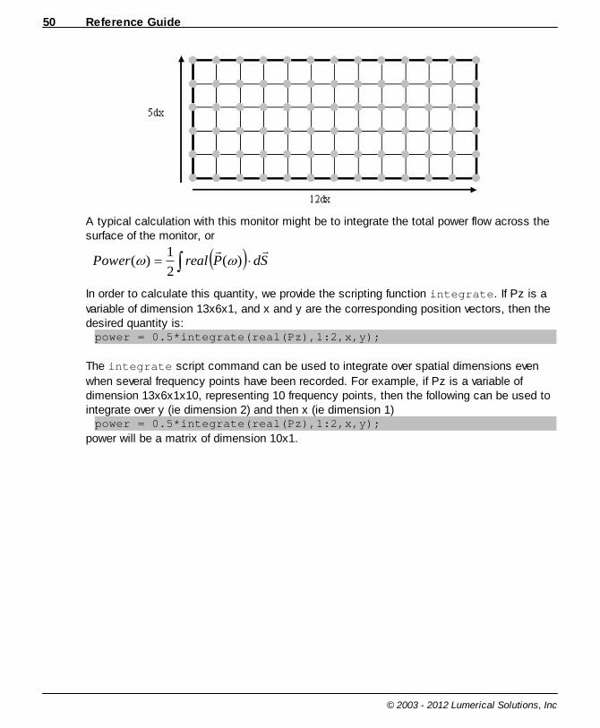
Reference Guide50
© 2003 - 2012 Lumerical Solutions, Inc
A typical calculation with this monitor might be to integrate the total power flow across thesurface of the monitor, or
SdPrealPower )(2
1)(
In order to calculate this quantity, we provide the scripting function integrate. If Pz is a
variable of dimension 13x6x1, and x and y are the corresponding position vectors, then thedesired quantity is:power = 0.5*integrate(real(Pz),1:2,x,y);
The integrate script command can be used to integrate over spatial dimensions even
when several frequency points have been recorded. For example, if Pz is a variable ofdimension 13x6x1x10, representing 10 frequency points, then the following can be used tointegrate over y (ie dimension 2) and then x (ie dimension 1)power = 0.5*integrate(real(Pz),1:2,x,y);
power will be a matrix of dimension 10x1.

CAD layout editor 51
© 2003 - 2012 Lumerical Solutions, Inc
4 CAD layout editor
The image below shows a typical Lumerical CAD Layout Editor. This tool is used to setupand analyze all simulations, and to run all script files.
In this screenshot,different regions of theCAD in Layout modeare highlighted. Theyinclude:
Main title barToolbarsView portsObject TreeOptimization andSweepsScript Prompt
The Layout Editor has two modes of operation: Layout mode and Analysis mode. Layoutmode is used to setup your simulation. Simulation objects can be added, modified anddeleted in this mode. After a simulation runs, the Layout Editor automatically switches toAnalysis mode. In analysis mode, it is not possible to edit the simulation objects, sincewe want the object settings to match the data from the simulation. To edit simulation
objects, switch back to layout mode with the button.
FDTD Solutions 8.0 features a new Results View window, which shows all the currentresults for the simulation object that is currently selected in the Object Tree. When used inconjunction with the Visualizer , it provides a very useful and intuitive way of analyzingand visualizing results through the GUI.
52
52
60
60
63
63
62
139

Reference Guide52
© 2003 - 2012 Lumerical Solutions, Inc
4.1 Main title barThe menus on the main title bar are listed below. If any of the options can be selectedusing a button on a toolbar, the icon is drawn to the left of the name. Similarly, shortcutkeys are located to the right.
File The file menu includes options to create, save and load simulation files. The Import menuallows users to import structural data stored in GDSII files files.
EditThe edit menu allows users to undo/redo their actions, and to copy/paste/edit object in thesimulation.
ViewThe view menu provides options to control the layout and visibility windows and toolbars.
SettingThis setting menu contains options to change the unit setting within the graphical interface. These option only apply to the GUI. Scripts always use SI units.
Simulation This menu contains settings for configuring resources and running simulations.
HelpThe help menu provides links to local PDF copies of the product documentation and linksto the larger set of online documentation, as well as options for checking which version of the software is installed.
4.2 ToolbarsThe following sections describe the various toolbars. Toolbars visibility can be controlled inthe View - Toolbars menu.
4.2.1 Main
The main toolbar contains buttons to add various Simulation objects, open the Materialdatabase and import files, as described below. When available, clicking the arrow to theright of the icon expands a drop-down menu containing related buttons. If one of the relatedbuttons is pressed, it replaces the default button in the toolbar. See the Simulation objectschapter for information about specific objects.
Material Database
77
116
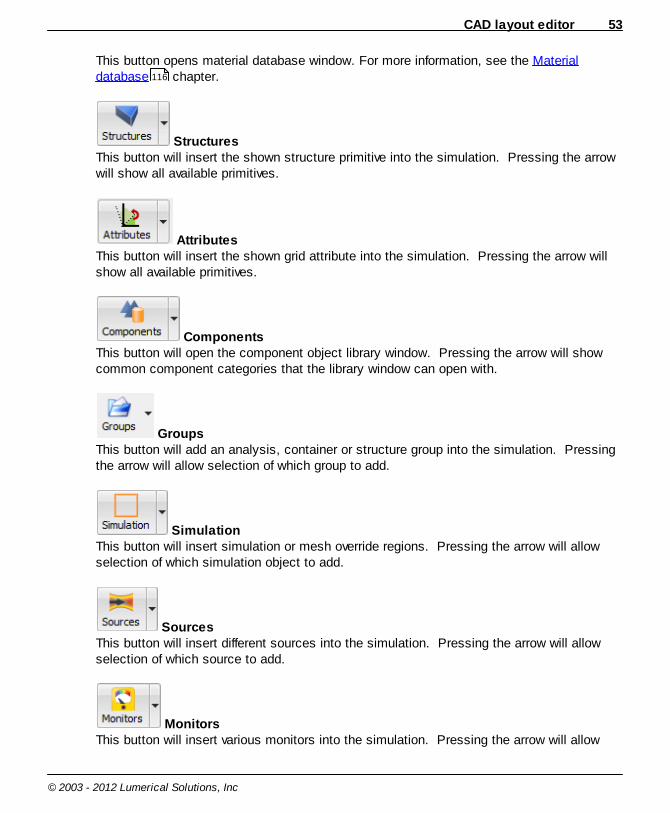
CAD layout editor 53
© 2003 - 2012 Lumerical Solutions, Inc
This button opens material database window. For more information, see the Materialdatabase chapter.
StructuresThis button will insert the shown structure primitive into the simulation. Pressing the arrowwill show all available primitives.
AttributesThis button will insert the shown grid attribute into the simulation. Pressing the arrow willshow all available primitives.
ComponentsThis button will open the component object library window. Pressing the arrow will showcommon component categories that the library window can open with.
GroupsThis button will add an analysis, container or structure group into the simulation. Pressingthe arrow will allow selection of which group to add.
SimulationThis button will insert simulation or mesh override regions. Pressing the arrow will allowselection of which simulation object to add.
SourcesThis button will insert different sources into the simulation. Pressing the arrow will allowselection of which source to add.
MonitorsThis button will insert various monitors into the simulation. Pressing the arrow will allow
116
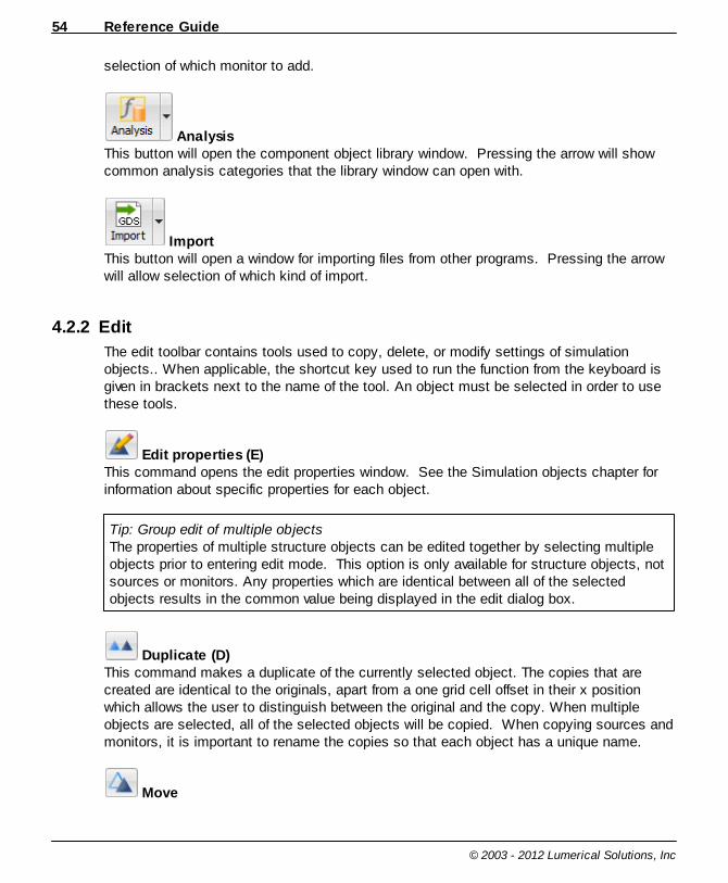
Reference Guide54
© 2003 - 2012 Lumerical Solutions, Inc
selection of which monitor to add.
AnalysisThis button will open the component object library window. Pressing the arrow will showcommon analysis categories that the library window can open with.
ImportThis button will open a window for importing files from other programs. Pressing the arrowwill allow selection of which kind of import.
4.2.2 Edit
The edit toolbar contains tools used to copy, delete, or modify settings of simulationobjects.. When applicable, the shortcut key used to run the function from the keyboard isgiven in brackets next to the name of the tool. An object must be selected in order to usethese tools.
Edit properties (E) This command opens the edit properties window. See the Simulation objects chapter forinformation about specific properties for each object.
Tip: Group edit of multiple objectsThe properties of multiple structure objects can be edited together by selecting multipleobjects prior to entering edit mode. This option is only available for structure objects, notsources or monitors. Any properties which are identical between all of the selectedobjects results in the common value being displayed in the edit dialog box.
Duplicate (D)This command makes a duplicate of the currently selected object. The copies that arecreated are identical to the originals, apart from a one grid cell offset in their x positionwhich allows the user to distinguish between the original and the copy. When multipleobjects are selected, all of the selected objects will be copied. When copying sources andmonitors, it is important to rename the copies so that each object has a unique name.
Move
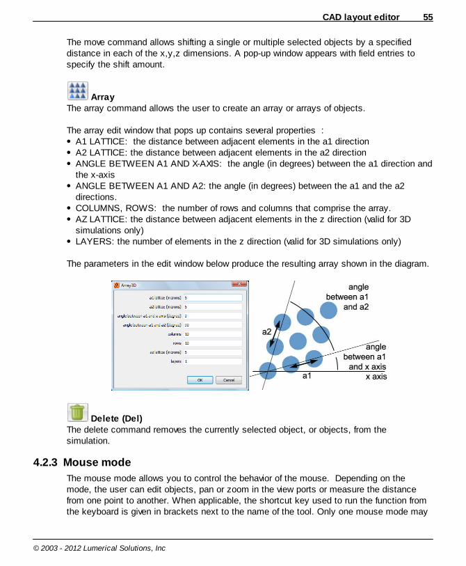
CAD layout editor 55
© 2003 - 2012 Lumerical Solutions, Inc
The move command allows shifting a single or multiple selected objects by a specifieddistance in each of the x,y,z dimensions. A pop-up window appears with field entries tospecify the shift amount.
ArrayThe array command allows the user to create an array or arrays of objects.
The array edit window that pops up contains several properties :A1 LATTICE: the distance between adjacent elements in the a1 directionA2 LATTICE: the distance between adjacent elements in the a2 directionANGLE BETWEEN A1 AND X-AXIS: the angle (in degrees) between the a1 direction andthe x-axisANGLE BETWEEN A1 AND A2: the angle (in degrees) between the a1 and the a2directions. COLUMNS, ROWS: the number of rows and columns that comprise the array.AZ LATTICE: the distance between adjacent elements in the z direction (valid for 3Dsimulations only)LAYERS: the number of elements in the z direction (valid for 3D simulations only)
The parameters in the edit window below produce the resulting array shown in the diagram.
Delete (Del)The delete command removes the currently selected object, or objects, from thesimulation.
4.2.3 Mouse mode
The mouse mode allows you to control the behavior of the mouse. Depending on themode, the user can edit objects, pan or zoom in the view ports or measure the distancefrom one point to another. When applicable, the shortcut key used to run the function fromthe keyboard is given in brackets next to the name of the tool. Only one mouse mode may
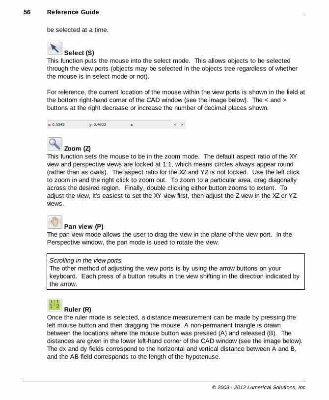
Reference Guide56
© 2003 - 2012 Lumerical Solutions, Inc
be selected at a time.
Select (S)This function puts the mouse into the select mode. This allows objects to be selectedthrough the view ports (objects may be selected in the objects tree regardless of whetherthe mouse is in select mode or not).
For reference, the current location of the mouse within the view ports is shown in the field atthe bottom right-hand corner of the CAD window (see the image below). The < and >buttons at the right decrease or increase the number of decimal places shown.
Zoom (Z)This function sets the mouse to be in the zoom mode. The default aspect ratio of the XYview and perspective views are locked at 1:1, which means circles always appear round(rather than as ovals). The aspect ratio for the XZ and YZ is not locked. Use the left clickto zoom in and the right click to zoom out. To zoom to a particular area, drag diagonallyacross the desired region. Finally, double clicking either button zooms to extent. Toadjust the view, it's easiest to set the XY view first, then adjust the Z view in the XZ or YZviews.
Pan view (P)The pan view mode allows the user to drag the view in the plane of the view port. In thePerspective window, the pan mode is used to rotate the view.
Scrolling in the view portsThe other method of adjusting the view ports is by using the arrow buttons on yourkeyboard. Each press of a button results in the view shifting in the direction indicated bythe arrow.
Ruler (R)Once the ruler mode is selected, a distance measurement can be made by pressing theleft mouse button and then dragging the mouse. A non-permanent triangle is drawnbetween the locations where the mouse button was pressed (A) and released (B). Thedistances are given in the lower left-hand corner of the CAD window (see the image below).The dx and dy fields correspond to the horizontal and vertical distance between A and B,and the AB field corresponds to the length of the hypotenuse.
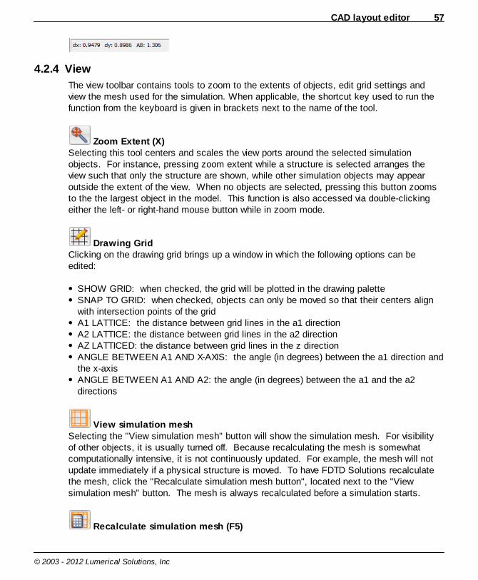
CAD layout editor 57
© 2003 - 2012 Lumerical Solutions, Inc
4.2.4 View
The view toolbar contains tools to zoom to the extents of objects, edit grid settings andview the mesh used for the simulation. When applicable, the shortcut key used to run thefunction from the keyboard is given in brackets next to the name of the tool.
Zoom Extent (X)Selecting this tool centers and scales the view ports around the selected simulationobjects. For instance, pressing zoom extent while a structure is selected arranges theview such that only the structure are shown, while other simulation objects may appearoutside the extent of the view. When no objects are selected, pressing this button zoomsto the the largest object in the model. This function is also accessed via double-clickingeither the left- or right-hand mouse button while in zoom mode.
Drawing GridClicking on the drawing grid brings up a window in which the following options can beedited:
SHOW GRID: when checked, the grid will be plotted in the drawing paletteSNAP TO GRID: when checked, objects can only be moved so that their centers alignwith intersection points of the gridA1 LATTICE: the distance between grid lines in the a1 directionA2 LATTICE: the distance between grid lines in the a2 directionAZ LATTICED: the distance between grid lines in the z directionANGLE BETWEEN A1 AND X-AXIS: the angle (in degrees) between the a1 direction andthe x-axisANGLE BETWEEN A1 AND A2: the angle (in degrees) between the a1 and the a2directions
View simulation meshSelecting the "View simulation mesh" button will show the simulation mesh. For visibilityof other objects, it is usually turned off. Because recalculating the mesh is somewhatcomputationally intensive, it is not continuously updated. For example, the mesh will notupdate immediately if a physical structure is moved. To have FDTD Solutions recalculatethe mesh, click the "Recalculate simulation mesh button", located next to the "Viewsimulation mesh" button. The mesh is always recalculated before a simulation starts.
Recalculate simulation mesh (F5)
Reference Guide58
© 2003 - 2012 Lumerical Solutions, Inc
Mesh generation is too computationally intensive to be done constantly as the simulationsetup is modified. If you wish to see the current mesh, use this option to update andrecalculate the mesh. The mesh is always recalculated before running a simulation.
4.2.5 Simulation
The simulation tools are:
ResourcesOpens the resource configuration manager. This window can add/remove and enable/disable computational resources. It also contains a useful configuration test tool to checkthe resource setup.
Check memory requirements This function will estimate the memory requirements for the current simulation. The totalrequirements are broken down into categories such as Simulation fields and Monitor data.
Material Explorer The Materials Explorer can be used to check the material's optical properties that will beused in a simulation. For more information, please see the section on Material Explorer.
Run parallel FDTD Run the current simulation in parallel mode. For more information on how to run simulation,see Running a simulation.
Run FDTDRun the current simulation in single process mode.
Run scripts This function will allow the user to run a Lumerical script file (*.lsf) to perform automated
commands such as plotting and saving data. This button is located in the CAD environmenttwice if the script editor is open: once in the simulation toolbar and once at the top of thescript editor. Pressing the button on the toolbar brings up an open file dialog. Pressing thebutton in the script editor runs the script that is selected in the editor window.
Switch to layout editor
125
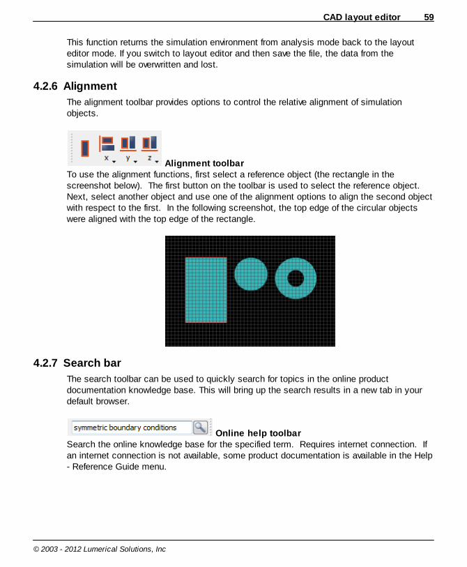
CAD layout editor 59
© 2003 - 2012 Lumerical Solutions, Inc
This function returns the simulation environment from analysis mode back to the layouteditor mode. If you switch to layout editor and then save the file, the data from thesimulation will be overwritten and lost.
4.2.6 Alignment
The alignment toolbar provides options to control the relative alignment of simulationobjects.
Alignment toolbarTo use the alignment functions, first select a reference object (the rectangle in thescreenshot below). The first button on the toolbar is used to select the reference object. Next, select another object and use one of the alignment options to align the second objectwith respect to the first. In the following screenshot, the top edge of the circular objectswere aligned with the top edge of the rectangle.
4.2.7 Search bar
The search toolbar can be used to quickly search for topics in the online productdocumentation knowledge base. This will bring up the search results in a new tab in yourdefault browser.
Online help toolbarSearch the online knowledge base for the specified term. Requires internet connection. Ifan internet connection is not available, some product documentation is available in the Help- Reference Guide menu.
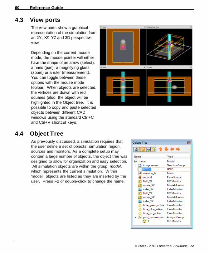
Reference Guide60
© 2003 - 2012 Lumerical Solutions, Inc
4.3 View portsThe view ports show a graphicalrepresentation of the simulation froman XY, XZ, YZ and 3D perspectiveview.
Depending on the current mousemode, the mouse pointer will eitherhave the shape of an arrow (select),a hand (pan), a magnifying glass(zoom) or a ruler (measurement).You can toggle between theseoptions with the mouse modetoolbar. When objects are selected,the vertices are drawn with redsquares (also, the object will behighlighted in the Object tree. It ispossible to copy and paste selectedobjects between different CADwindows using the standard Ctrl+Cand Ctrl+V shortcut keys.
4.4 Object TreeAs previously discussed, a simulation requires thatthe user define a set of objects, simulation region,sources and monitors. As a complete setup maycontain a large number of objects, the object tree wasdesigned to allow for organization and easy selection. All simulation objects are within the group, model,which represents the current simulation. Within'model', objects are listed as they are inserted by theuser. Press F2 or double-click to change the name.

CAD layout editor 61
© 2003 - 2012 Lumerical Solutions, Inc
To move the objects up and down the tree as well as into groups, we use the orange arrowsat the top of the window. The up and down arrows shift the objects relative to each other,while the left and right arrows move them out of and into groups. To add groups, we usethe button called groups in the main toolbar. Structure groups can only contain structuresand likewise, analysis groups can only contain monitors. See the online user guide sectionfor more information and examples about Structure groups and Analysis groups. The thirdgroup, "Containers" act like folders and can hold any type of object. In the image above,the 'Sources/Monitors' container group has both individual sources and monitors as well asan analysis group.
Note that there are buttons with green crosses at the top of the objects tree. These buttonscan be used to hide or display certain types of objects. When objects are selected, theyare highlighted blue in the objects tree and the vertices are marked with red squares in theview ports. Objects can always be selected by left-clicking on their name in the object treeor edited by right-clicking. Using the tree is the preferred method of selection especially incomplicated simulation setups with many overlapping elements. In the image above, thepower monitor, above, is selected.
4.4.1 Enable/Disable Simulation Object
User can enable/disable simulation objects by right-clicking on each and selecting"Enable/Disable". Disabled simulation objects will remain in the object tree (and can bere-enabled), they will have no effect on the simulation.
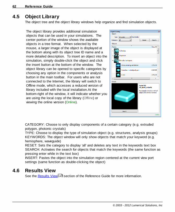
Reference Guide62
© 2003 - 2012 Lumerical Solutions, Inc
4.5 Object LibraryThe object tree and the object library windows help organize and find simulation objects.
The object library provides additional simulationobjects that can be used in your simulations. Thecenter portion of the window shows the availableobjects in a tree format. When selected by themouse, a larger image of the object is displayed atthe bottom along with its object tree ID name and amore detailed description. To insert an object into thesimulation, simply double-click the object and clickthe insert button at the bottom of the window. Theobject library can be opened to specific categories bychoosing any option in the components or analysisbutton in the main toolbar. For users who are notconnected to the Internet, the library will switch toOffline mode, which accesses a reduced version oflibrary included with the local installation.At thebottom-right of the window, it will indicate whether youare using the local copy of the library (Offline) orviewing the online version (Online).
CATEGORY: Choose to only display components of a certain category (e.g. extrudedpolygon, photonic crystals)TYPE: Choose to display the type of simulation object (e.g. structures, analysis groups)KEYWORDS: The object window will only show objects that match your keyword (e.g.hemisphere, waveguide)RESET: Sets the category to display 'all' and deletes any text in the keywords text boxSEARCH: Activates the search for objects that match the keywords (the same function aspressing enter while in the text box)INSERT: Pastes the object into the simulation region centered at the current view portsettings (same function as double-clicking the object)
4.6 Results ViewSee the Results View section of the Reference Guide for more information.143
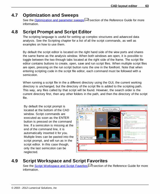
CAD layout editor 63
© 2003 - 2012 Lumerical Solutions, Inc
4.7 Optimization and SweepsSee the Optimization and parameter sweeps section of the Reference Guide for moreinformation.
4.8 Script Prompt and Script EditorThe scripting language is useful for setting up complex structures and advanced dataanalysis. See the Scripting chapter for a list of all the script commands, as well asexamples on how to use them.
By default the script editor is located on the right hand side of the view ports and sharesthe same frame as the analysis window. When both windows are open, it is possible totoggle between the two through tabs located at the right side of the frame. The script fileeditor contains buttons to create, open, save and run script files. When multiple script filesare open, pressing on the run script button runs the one in the forefront. Note that whenentering scripting code in the script file editor, each command must be followed with asemicolon.
When running a script file in the a different directory using the GUI, the current workingdirectory is unchanged, but the directory of the script file is added to the scripting path.This way, any files called by that script will be found. However, the search order is thecurrent directory first, then any other folders in the path, and then the directory of the scriptfile.
By default the script prompt islocated at the bottom of the CADwindow. Script commands areexecuted as soon as the ENTERbutton is pressed on the commandline. If a semicolon is missing at theend of the command line, it isautomatically inserted it for you.Multiple lines can be pasted into thescript prompt, and will run as in thescript editor. In this case though,only the last semicolon can beneglected.
4.9 Script Workspace and Script FavoritesSee the Script Workspace and Script Favorites section of the Reference Guide for moreinformation.
146
144
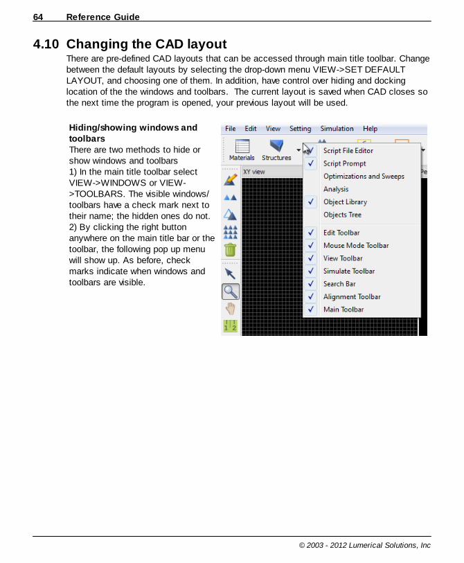
Reference Guide64
© 2003 - 2012 Lumerical Solutions, Inc
4.10 Changing the CAD layoutThere are pre-defined CAD layouts that can be accessed through main title toolbar. Changebetween the default layouts by selecting the drop-down menu VIEW->SET DEFAULTLAYOUT, and choosing one of them. In addition, have control over hiding and dockinglocation of the the windows and toolbars. The current layout is saved when CAD closes sothe next time the program is opened, your previous layout will be used.
Hiding/showing windows andtoolbarsThere are two methods to hide orshow windows and toolbars1) In the main title toolbar selectVIEW->WINDOWS or VIEW->TOOLBARS. The visible windows/toolbars have a check mark next totheir name; the hidden ones do not.2) By clicking the right buttonanywhere on the main title bar or thetoolbar, the following pop up menuwill show up. As before, checkmarks indicate when windows andtoolbars are visible.
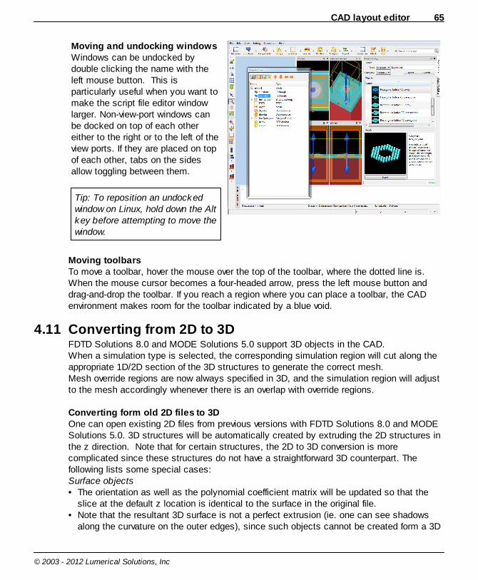
CAD layout editor 65
© 2003 - 2012 Lumerical Solutions, Inc
Moving and undocking windowsWindows can be undocked bydouble clicking the name with theleft mouse button. This isparticularly useful when you want tomake the script file editor windowlarger. Non-view-port windows canbe docked on top of each othereither to the right or to the left of theview ports. If they are placed on topof each other, tabs on the sidesallow toggling between them.
Tip: To reposition an undockedwindow on Linux, hold down the Altkey before attempting to move thewindow.
Moving toolbarsTo move a toolbar, hover the mouse over the top of the toolbar, where the dotted line is.When the mouse cursor becomes a four-headed arrow, press the left mouse button anddrag-and-drop the toolbar. If you reach a region where you can place a toolbar, the CADenvironment makes room for the toolbar indicated by a blue void.
4.11 Converting from 2D to 3DFDTD Solutions 8.0 and MODE Solutions 5.0 support 3D objects in the CAD. When a simulation type is selected, the corresponding simulation region will cut along theappropriate 1D/2D section of the 3D structures to generate the correct mesh.Mesh override regions are now always specified in 3D, and the simulation region will adjustto the mesh accordingly whenever there is an overlap with override regions.
Converting form old 2D files to 3D One can open existing 2D files from previous versions with FDTD Solutions 8.0 and MODESolutions 5.0. 3D structures will be automatically created by extruding the 2D structures inthe z direction. Note that for certain structures, the 2D to 3D conversion is morecomplicated since these structures do not have a straightforward 3D counterpart. Thefollowing lists some special cases:Surface objects• The orientation as well as the polynomial coefficient matrix will be updated so that the
slice at the default z location is identical to the surface in the original file.• Note that the resultant 3D surface is not a perfect extrusion (ie. one can see shadows
along the curvature on the outer edges), since such objects cannot be created form a 3D

Reference Guide66
© 2003 - 2012 Lumerical Solutions, Inc
surface.Structure groups• A new property “z_span” is added in the User properties section with the default setting
of 1 unit length.Import surfaces• Since import surfaces are now defined as z(x,y) instead of y(x), there will be some
changes to the Geometry tab as well as an additional rotation so that the 3D objectlooks like an extrusion in the z direction.
The default option sets the z location at 0 and the z span as 1 unit length. The simulationregion will be placed at the center of the object in the z direction and the resultant meshedstructure (in the simulation region) will be identical to the original 2D file. New simulationobjects are created based on the default values set in Setting->Set default objectplacement. Note that since 3D objects require more memory to render, it is important notto use too high of a resolution for the graphical rendering, or the CAD may slow downsignificantly.
2D DRAW MODEOne can use the 2D draw mode to enable a layout that looks very similar to that of 2DFDTD Solutions or MODE Solutions 4.0. This option can be selected from View->Setdefault layout -> 2D -> XY/XZ/YZ, and all but the selected view port will be closed.
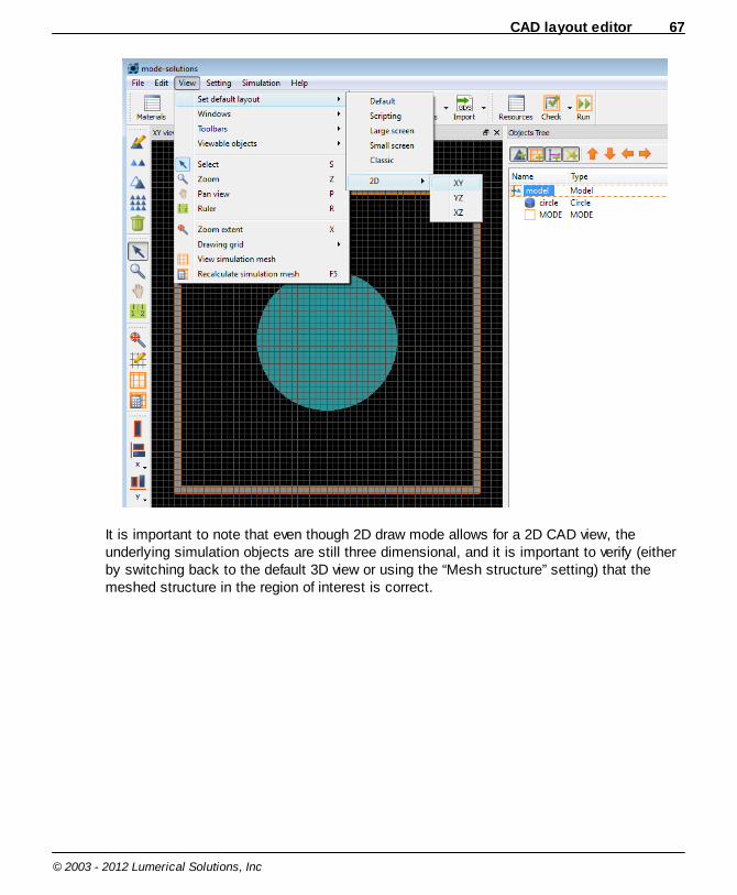
CAD layout editor 67
© 2003 - 2012 Lumerical Solutions, Inc
It is important to note that even though 2D draw mode allows for a 2D CAD view, theunderlying simulation objects are still three dimensional, and it is important to verify (eitherby switching back to the default 3D view or using the “Mesh structure” setting) that themeshed structure in the region of interest is correct.
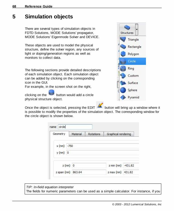
Reference Guide68
© 2003 - 2012 Lumerical Solutions, Inc
5 Simulation objects
There are several types of simulation objects inFDTD Solutions, MODE Solutions' propagator,MODE Solutions' Eigenmode Solver and DEVICE.
These objects are used to model the physicalstructure, define the solver region, any sources oflight or doping/generation regions as well asmonitors to collect data.
The following sections provide detailed descriptionsof each simulation object. Each simulation objectcan be added by clicking on the correspondingicon in the GUI.For example, in the screen shot on the right,
clicking on the button would add a circlephysical structure object.
Once the object is selected, pressing the EDIT button will bring up a window where itis possible to modify the properties of the simulation object. The corresponding window forthe circle object is shown below.
TIP: In-field equation interpreterThe fields for numeric parameters can be used as a simple calculator. For instance, if you
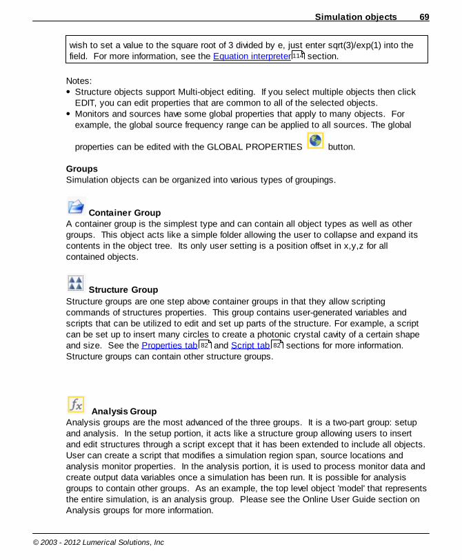
Simulation objects 69
© 2003 - 2012 Lumerical Solutions, Inc
wish to set a value to the square root of 3 divided by e, just enter sqrt(3)/exp(1) into thefield. For more information, see the Equation interpreter section.
Notes:Structure objects support Multi-object editing. If you select multiple objects then clickEDIT, you can edit properties that are common to all of the selected objects.Monitors and sources have some global properties that apply to many objects. Forexample, the global source frequency range can be applied to all sources. The global
properties can be edited with the GLOBAL PROPERTIES button.
GroupsSimulation objects can be organized into various types of groupings.
Container GroupA container group is the simplest type and can contain all object types as well as othergroups. This object acts like a simple folder allowing the user to collapse and expand itscontents in the object tree. Its only user setting is a position offset in x,y,z for allcontained objects.
Structure Group Structure groups are one step above container groups in that they allow scriptingcommands of structures properties. This group contains user-generated variables andscripts that can be utilized to edit and set up parts of the structure. For example, a scriptcan be set up to insert many circles to create a photonic crystal cavity of a certain shapeand size. See the Properties tab and Script tab sections for more information.Structure groups can contain other structure groups.
Analysis GroupAnalysis groups are the most advanced of the three groups. It is a two-part group: setupand analysis. In the setup portion, it acts like a structure group allowing users to insertand edit structures through a script except that it has been extended to include all objects.User can create a script that modifies a simulation region span, source locations andanalysis monitor properties. In the analysis portion, it is used to process monitor data andcreate output data variables once a simulation has been run. It is possible for analysisgroups to contain other groups. As an example, the top level object 'model' that representsthe entire simulation, is an analysis group. Please see the Online User Guide section on Analysis groups for more information.
114
82 82

Reference Guide70
© 2003 - 2012 Lumerical Solutions, Inc
The purpose of this section of the Reference Guide is to describe all of the availablesimulation objects and their properties. This section is organized as follows. There are fivesubsections. The first four subsections correspond to the four types of object categories.Each of these sections begins with a brief overview of the simulation objects followed by adescription of their property settings. The properties are organized according to the tab thatthey are located in when the EDIT button is pressed. The last of the five subsectionsdescribes the syntax for the equation interpreter.
5.1 StructuresStructures in a simulation interact with light/electrical sources to produce interestingeffects. They are split into 3 groups:
Structures (Primitives)These are the primitive shapes that make up all structure setups.
AttributesThese are the additional attributes that can be associated with any structure.
ComponentsThese are preset structures and more complicated structure groups that are commonlyused in a variety of research areas. Components are built using the group script and haveuser settable parameters. They form a collection of samples from which to build your ownstructure groups.
ImportsThese options open windows that can be used to import structure data from other sourcessuch as pictures or text files.

Simulation objects 71
© 2003 - 2012 Lumerical Solutions, Inc
5.1.1 Primitives
The button includes options to to add the following primitive structures:
TriangleTriangular objects denote physical objects that appear triangular from above. For 2Dsimulations, these objects represent triangles while in 3D these objects are extruded in thez direction to a specific height. They are actually polygon objects, with the number ofvertices set to 3.
RectangleRectangular regions denote physical objects that appear rectangular from above. For 2Dsimulations, these objects represent rectangles while in 3D these objects are extruded to aspecific height.
Polygon Polygons allow the user to define a custom object with a variable number of vertices. Thelocation of each vertex can be independently positioned within a plane, and the vertices areconnected with straight lines. For 3D simulations, the object is extruded in the zdimension.
CircleCircles denote physical objects which appear circular or ellipsoid from above. They areeither circles/ellipses in 2D, or circular/ellipsoid cylinders in 3D.
RingRing regions represent physical objects that consist of full or partial rings when viewed fromabove. Rings in 3D simulations are extruded in the z direction to a specific height.
Custom Primitives Custom primitives can be used to create customized surfaces, specified via parametricequations. The resulting surfaces can either exist on one or more faces of the object, orcan be used to define a cylindrically-symmetric surface of revolution.

Reference Guide72
© 2003 - 2012 Lumerical Solutions, Inc
Surface Surface primitives can be used to define complex material volumes that exist above orbelow analytically defined surfaces. In 3D simulations, a surface (S) is defined as a functionof variables u and v, i.e. S = S(u,v). The variables (u,v) can represent (x,y), (x,z) or (y,z)depending on the surface orientation. Similarly, in 2D simulations, a surface is defined as afunction of u (S = S(u)) where u can represent x or y.
Sphere In 3D simulations, users can define spherical regions of constant refractive index throughthe spherical physical object. Spherical objects only exist in 3D simulations.
Pyramid Pyramids can be configured to half flat tops and/or flat bottoms, and either narrow orexpand in the vertical z direction. Pyramids are only available for 3D simulations.
5.1.2 Attributes
The button includes options to add the following attributes:
Permittivity rotationThe permittivity rotation grid attribute allows users to add an arbitrary Euler rotation to thedielectric tensor. The main parameters are the "angle convention" and the Euler anglestheta/phi/psi.
LC orientationThe LC orientation grid attribute allows users to specify arbitrary orientations for the LiquidCrystal director. The main parameters are the angles theta/pi (specifying the LCorientation), and the dielectric tensor will be set accordingly.
Matrix transformThe matrix transform grid attribute allows users to add an arbitrary unitary matrix to thedielectric tensor. The main parameter is the unitary matrix U.
For examples on how to use the grid attributes listed above, see the Anisotropy andMagneto-Optics section of the Applications Library.
Simulation objects 73
© 2003 - 2012 Lumerical Solutions, Inc
5.1.3 Components
The button includes options to open the object library with a few presetcategories. Components are more complicated structures that are built from one or severalprimitives. Common parameters are available to be adjusted. These pre-built structuregroups enable users to quickly setup common (but often difficult to construct), simulationenvironments.
The preset categories are:
Extruded polygonsPolygons allow the user to define a custom object with a variable number of vertices. Thelocation of each vertex can be independently positioned within a plane, and the vertices areconnected with straight lines. These shapes are extruded in the z dimension.
Integrated optics This category includes various shapes of waveguide paths. For 3D simulations, thesidewalls can be vertical or angled.
Photonic crystalsPhotonic crystals are optical nanostructures that are either rectangular or hexagonalperiodic. This category includes PC waveguides and PC cavities.
GratingsGratings are a regularly spaced set of elements which can have polarizing, reflecting, orcoupling effects.
SurfaceThis category contains examples of surface objects defined by equations.
More choicesThere are many more categories of components available that are constantly beingupdated.

Reference Guide74
© 2003 - 2012 Lumerical Solutions, Inc
5.1.4 Geometry tab
The geometry tab contains options to change the size and location of the structure.
5.1.5 Material tab
The material options are as follows:
MATERIAL: This field can be set to any material included in the material database. It ispossible to include new materials in the database, or edit the materials already included.See the material database section for more information.
If <Object defined dielectric> is selected, then the index property must be set.INDEX: The refractive index of the structure, when the material type is <Object defineddielectric>. The index must be greater than one, and can be specified as an equation interms of x, y, z(defined in the Equation interpreter section). If specifying ananisotropic material, use a semicolon to separate the x,y,z indices. Eg. 1;1.5;1INDEX UNITS: The field specifies the units of the spatial variables only when the index isspecified with a formula (the origin is the center of the object). The units will affect theinterpretation of l0 and k0.
OVERRIDE MESH ORDER FROM MATERIAL DATABASE: Select to override the meshorder from the material database and manually set a mesh order. The mesh order isused by the simulation engine to select which material to use when two materialsoverlap. See the mesh order section for more details. MESH ORDER: Set the mesh order in this field if the OVERRIDE MESH ORDER FROMMATERIAL DATABASE option is selected. If the option is not selected, the field displaysthe material's default mesh order from the database. For example, a material of meshorder 1 will take precedence over a material of mesh order 2.
5.1.6 Rotations tab
Rotate objects by setting the following variables:
FIRST, SECOND, THIRD AXES: 3D simulation only. Select rotation axis. Up to threedifferent rotations can be applied. ROTATION 1,2,3: The rotation of the object in a clockwise direction about each axis,measured in degrees. In 2D simulation, only one angle (rotated around z axis) isavailable.
5.1.7 Graphical Rendering tab
The graphical rendering tab is used to change how objects are drawn in the layout editor.The options are:
RENDER TYPE: The options for drawing the objects are detailed or wireframe. Detailed
114
127
Simulation objects 75
© 2003 - 2012 Lumerical Solutions, Inc
objects are shaded and their transparency can be set using OVERRIDE COLOROPACITY FROM MATERIAL DATABASE.DETAIL: This is a slider which takes values between 0 and 1. By default it is set to 0.5.Higher detail shows more detail, but increases the time required to draw objects. Thissetting has no effect on the simulation.OVERRIDE COLOR OPACITY FROM MATERIAL DATABASE: When unselected theopacity is determined from the material database. When selected, you can specify avalue for ALPHA between 0 (transparent) and 1 (opaque) for the object, depending onhow transparent you want the object to be.
5.1.8 Custom tab
The custom tab is only available for custom primitives. Custom primitives are objects thatare defined by equations describing the boundaries of the physical object. The customprimitive defaults to a rectangular region upon creation, and is shaped via entry of one ormore equations in the edit window.
The custom object allows you to define the y position of the object as a function of the xposition. The z position is obtained via extrusion or revolution of the y edge. (X,Y)=(0,0)corresponds to the center of the object.
EQUATION 1: The equation, expressed as a function of x, which defines the upper yedge of the physical object. The origin of equation is the center of the object. Suitablesyntax for the equations is shown in the Equation interpreter section.MAKE NONSYMMETRIC: Uncheck this if you want to define the lower edge with adifferent equation.EQUATION 2: The equation, expressed as a function of x, which defines the lower edgeof the physical object. EQUATION UNITS: The default units in which x and y are expressed in equation 1 and 2.For example, a setting of microns means that both x and y are expressed in microns. CREATE 3D OBJECT BY: Options include "extrusion", and "revolution". Extrusionresults in an object that is extruded along the z-axis (i.e. invariant in z). The revolutionobject is created by revolving the equation around the x-axis, resulting in a surface ofrevolution.
Equation 1 and 2 are bound such that they are only defined over specific regions.Equations which result in undefined values (1/0) result in a zero height; any equation leftblank results in a custom primitive of zero height everywhere. Equations that go larger thanthe span of the object will be clipped at the edge of the object. Equations that go negativewill be clipped at zero. In the following figure, notice how the equations are clipped at theedge of the object.
114

Reference Guide76
© 2003 - 2012 Lumerical Solutions, Inc
5.1.9 Import Data tab
The button includes options to import from a variety of formats:
GDSIIThis file format is commonly used to store 2-dimensional geometric data. For details, see GDSII Import .
SurfacesFor example, this tool is useful for importing data from an atomic force microscope (AFM).In two dimensional simulations, the data must be defined as y = f(x). In three dimensionalsimulations, it must be defined as z = f(x,y). Both upper and lower surfaces can beimported.
ImagesIn either JPG or PNG format. For example, this tool is useful for importing from a scanningelectron microscope (SEM) image. In three dimensions, the imported data is extrudedalong the z axis.
(n,k) material The REFRACTIVE INDEX (N AND K) as a function of space, for example, to representdoped material where the doping concentrations and optical loss are calculated in anothersoftware package. In two dimensions, the data is defined as n(x,y), k(x,y) and in threedimensions as n(x,y,z), k(x,y,z). Please note that the value of k is translated into aconductive (or plasma) model and is only valid at a the center frequency of the simulation. It
77

Simulation objects 77
© 2003 - 2012 Lumerical Solutions, Inc
should therefore only be used with single frequency simulations.
5.1.9.1 GDSII Import
The GDSII import function allows you to import structures from a GDSII file into the layouteditor. The GDSII file format is commonly used to store 2-dimensional geometric data. Thisdata can be directly imported into a 2D layout environment, or it can be used to import 3Dobjects into a 3D layout environment by extruding the 2D data in the Z dimension.
Characteristics of the GDSII fileLumerical products support most, but not all features of the GDSII file format. Unsupportedfeatures should not prevent the file from being imported, however, the results may not be asexpected. The following table details the supported and unsupported features.
Features Supported
General
Multiple cells in GDSII library file Yes
Layer numbers for drawing objects Yes
Primitives/Objects
Box/Rectangle Yes
Polygon Yes
Path (see note below) Yes
Node No
Text No
Symbolic cell reference Yes
Array cell reference Yes
Advanced
Cell references in external library/file No
Magnifications in array and symbolic Yes
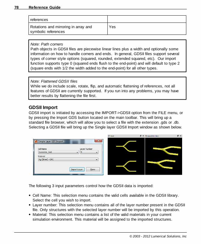
Reference Guide78
© 2003 - 2012 Lumerical Solutions, Inc
references
Rotations and mirroring in array andsymbolic references
Yes
Note: Path cornersPath objects in GDSII files are piecewise linear lines plus a width and optionally someinformation on how to handle corners and ends. In general, GDSII files support severaltypes of corner style options (squared, rounded, extended squared, etc). Our importfunction supports type 0 (squared ends flush to the end-point) and will default to type 2(square ends with 1/2 the width added to the end-point) for all other types.
Note: Flattened GDSII filesWhile we do include scale, rotate, flip, and automatic flattening of references, not allfeatures of GDSII are currently supported. If you run into any problems, you may havebetter results by flattening the file first.
GDSII Import GDSII import is initiated by accessing the IMPORT->GDSII option from the FILE menu, orby pressing the Import GDS button located on the main toolbar. This will bring up astandard file browser, which will allow you to select a file with the extension .gds or .db.Selecting a GDSII file will bring up the Single layer GDSII Import window as shown below.
The following 3 input parameters control how the GDSII data is imported:
Cell Name: This selection menu contains the valid cells available in the GDSII library.Select the cell you wish to import.Layer number: This selection menu contains all of the layer number present in the GDSIIfile. Only structures with the selected layer number will be imported by this operation.Material: This selection menu contains a list of the valid materials in your currentsimulation environment. This material will be assigned to the imported structures.

Simulation objects 79
© 2003 - 2012 Lumerical Solutions, Inc
Selecting the Import layer button imports all the structures with the selected layer numberin the selected cell into the layout environment. These structures are automatically insertedinto a structure group. The material is set as an input parameter for the structure code, andthe script in the structure group sets all the objects to the desired material. The name ofthe structure group includes the original number of layers. For 3D simulations, the structuregroup contains a variable "z span". This used to set the width of the layer in the z direction.The origin of the structures, as well as their orientation, can be changed by changing theproperties of the structure group.
5.1.9.2 nk material import window
Options in the (n,k) material import window include:
SELECT FILE: let the user specify the data file to be imported.X0, Y0, Z0: the data origin in the global coordinates of the Graphical Layout Editor.X SPAN, Y SPAN, Z SPAN: This defines the size of volume that you are importing.These fields are inactive and help to determine that the file units have been properlychosen.FILE UNITS: Select units for the data in your file.IMPORT AS Mji INSTEAD OF Mij: 2D simulation only. It is often easy to cycle throughthe array indices in the wrong order when exporting the file, and this check button allowsyou to reverse the order easily. Typically, it is very easy to see in the figure window whenyou have the order incorrect.IMPORT AS Mkji INSTEAD OF Mijk: 3D simulation only. It is often easy to cyclethrough the array indices in the wrong order when exporting the file, and this checkbutton allows you to reverse the order easily. Typically, it is very easy to see in the figurewindow when you have the order incorrect.PLOT PLANE: You can image the data in either the x-y plane, the x-z plane or the y-zplane to be sure that it is correctly imported. Use this menu chooser to switch betweenplanes.Z (or X or Y): Depending on the PLOT PLANE chosen, you can view cross sections atany depth into the structure. Use this slider or the value input field to choose the depth ofcross section.IMAGE N, IMAGE K: Choose to view n or k in the figure window.
For detailed information and example text import files, as well as script files that generatethe example files, see the Import object spatial (n,k) data page in the User Guide section ofthe Online help.

Reference Guide80
© 2003 - 2012 Lumerical Solutions, Inc
5.1.9.3 Surface import window
Options in the surface import window include:
SELECT FILE: let the user specify the data file to be imported.X0, Y0, Z0: the data origin in the global coordinates of the Graphical Layout Editor.X SPAN: This defines the length of surface that you are importing. If the x data wascontained in the file (file format type 1), then this field is inactive. If the x data was not inthe file, then this field is active and should be set to the desired data span.YSPAN: 3D simulation only. This defines the size of surface area that you are importing.INVERT X AND Y AXIS: It is often easy to invert the x and y axis when exporting the file.Selecting this checkbox means that the x and y axes are automatically reversed.UPPER SURFACE, LOWER SURFACE: Choose which surface is being imported.FILE UNITS: Select units for the data in your file.
For detailed information and example text import files, as well as script files that generatethe example files, see the Import object surfaces page in the User Guide section of theOnline help.
5.1.10 Surface tab
The diagrams below show how the surface is used to create a volume of desired material.
The surface equation can contain up to three terms, conic, polynomial and custom whichare added together to create the total surface. Not all terms have to be included.
custompolynomialconic SSSS
Conic term:
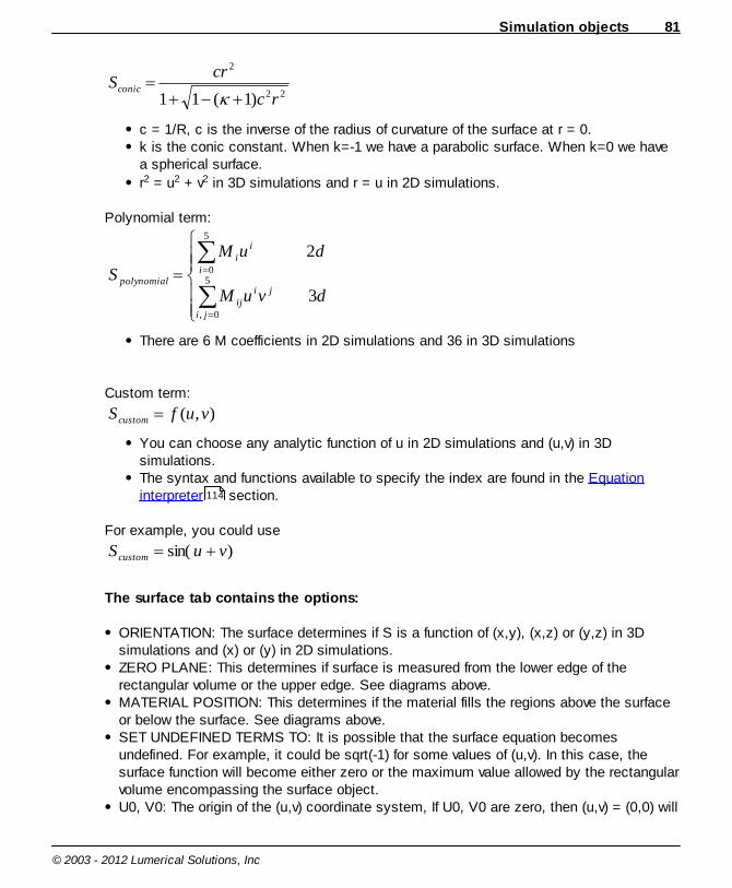
Simulation objects 81
© 2003 - 2012 Lumerical Solutions, Inc
22
2
)1(11 rc
crSconic
c = 1/R, c is the inverse of the radius of curvature of the surface at r = 0. k is the conic constant. When k=-1 we have a parabolic surface. When k=0 we havea spherical surface.
r2 = u2 + v2 in 3D simulations and r = u in 2D simulations.
Polynomial term:
dvuM
duM
Sji
jiij
i
ii
polynomial
3
2
5
0,
5
0
There are 6 M coefficients in 2D simulations and 36 in 3D simulations
Custom term:
),( vufScustom
You can choose any analytic function of u in 2D simulations and (u,v) in 3Dsimulations. The syntax and functions available to specify the index are found in the Equationinterpreter section.
For example, you could use
)sin( vuScustom
The surface tab contains the options:
ORIENTATION: The surface determines if S is a function of (x,y), (x,z) or (y,z) in 3Dsimulations and (x) or (y) in 2D simulations. ZERO PLANE: This determines if surface is measured from the lower edge of therectangular volume or the upper edge. See diagrams above. MATERIAL POSITION: This determines if the material fills the regions above the surfaceor below the surface. See diagrams above. SET UNDEFINED TERMS TO: It is possible that the surface equation becomesundefined. For example, it could be sqrt(-1) for some values of (u,v). In this case, thesurface function will become either zero or the maximum value allowed by the rectangularvolume encompassing the surface object. U0, V0: The origin of the (u,v) coordinate system, If U0, V0 are zero, then (u,v) = (0,0) will
114

Reference Guide82
© 2003 - 2012 Lumerical Solutions, Inc
correspond to the center of the surface object. Setting these values to non-zero will offsetthe origin by a desired amount.SURFACE UNITS: All quantities defining the surface must be measured in the sameunits. You can choose these units with this menu. CONIC: Check this option to include the conic term in the surface equation. If this ischecked, then set
RADIUS OF CURVATURE: curvature of the surface at the origin. This is equal to theinverse of the parameter c described in the definition of S
conic.
CONIC CONSTANT: The constant. CUSTOM: Check this option to include the custom term in the surface equation
EQUATION: The equation as a function of u in 2D simulations or u and v in 3Dsimulations.
POLYNOMIAL: Check this option to include a polynomial term in the surface equation. Ifthis option is checked, the M coefficients as explained above can be entered into a table.
5.1.11 Properties tab
The properties tab is only available for structure groups. The properties tab is used to setthe origin of the group, and to create the custom properties of the group that are the inputsof the group script. Custom user property variables may be added with the ADD button,and removed with the REMOVE button. Each user property has a name and a type(number, frequency ect). The user properties can be set manually in the edit GUI or throughscript commands. For more information and examples, see the Structure groups page ofthe User Guide section of the Online Help.
5.1.12 Script tab
The script tab is only available for structure groups. The script tab can contain scriptcommands that are used to set up a structure or edit the properties of structures locatedwithin the structure group. The structure group has access to the user variables defined inthe PROPERTIES tab, and can change properties of any objects that are contained in thegroup. The script does not have access to objects which are not located in the group, anddoes not share the same variable space as the script prompt.
The script is run every time the TEST or OK button is pressed, or when one of the userproperties is changed with a script command.
The following buttons and regions are available in the script tab:SCRIPT: This is where the script commands are written. To find a list of scriptcommands, see the Scripting Language section of the Reference Guide.TEST/SCRIPT OUTPUT: Press the TEST button to run the script. If there are no syntaxerrors in the script the SCRIPT OUTPUT will read <script complete>.
For more information and examples, see the Structure groups page of the User Guide
155

Simulation objects 83
© 2003 - 2012 Lumerical Solutions, Inc
section of the Online Help.
5.2 SimulationSimulation objects are used to define simulation parameters like boundary conditions andmesh size.
Simulation regionThe simulation region defines most simulation parameters including the size and meshsize.
Mesh override regionThe mesh override region is used to override the default mesh size in some part of thesimulation region. Normally the meshing parameters are set in the Simulation region. However, if some specific meshing conditions are required in part of the simulation region, amesh override region can be specified. For example, some simulations with metals arevery sensitive to meshing, and a mesh override region may be required at the metalsurface.
Note that only one simulation region per simulation is supported, but multiple mesh overrideregions may be used.
TIP: Objects which lie outside the simulation region.Any simulation objects contained or partly contained within the simulation region areincluded in the simulation, while any objects which fall completely outside of thesimulation region are not included in the simulation. Those physical structures (andportions thereof) lying within the simulation region are included in the simulation (i.e. thesimulation is performed on that portion of the physical structure lying within the simulationregion). Physical monitors and sources are treated in a similar fashion, such that anyportion of a monitor or source lying within a simulation region will be used. The user iswarned when at least one source or monitor falls completely outside the simulationregion.
5.2.1 General tab
The options in the general tab depend on whether the item being edited is a simulationregion or a mesh refinement region.
Simulation regionThe simulation region contains three settings:

Reference Guide84
© 2003 - 2012 Lumerical Solutions, Inc
DIMENSION: The dimension of the simulation region (2D or 3D). BACKGROUND INDEX: The refractive index of the surrounding, background medium inthe simulation region. SIMULATION TIME: The maximum duration of the simulation to be performed. The actualsimulation may be shorter if the autoshutoff criteria are satisfied before this maximumsimulation time is exceeded. For more information about how to choose the simulationtime see set the simulation region section of the introduction in the Getting Startedguide.
Mesh override region For the mesh override region the general tab includes options to override the mesh indifferent directions, and enter the desired maximum mesh spacing. Alternatively, since themesh spacing is usually determined by the refractive index of the materials in thesimulation, it is possible to set an EQUIVALENT INDEX that will be used to determine themesh spacing. A higher index will lead to a finer mesh.
5.2.2 Geometry tab
The geometry tab contains options to change the size and location of the simulation ormesh refinement region.
5.2.3 Mesh settings tab
The mesh settings tab includes settings that control the mesh geometry and thediscretization of time when relevant. There are three different types of meshes. The optionsfor each are described in more detail below. Then, the time step options are discussed forFDTD Solutions/Propagator simulations.
Auto non-uniformThe default setting. A non-uniform mesh is automatically generated based on the meshaccuracy slider bar and the material properties. Areas with a high index will have a smallermesh step size.
The MESH ACCURACY parameter is an integer from 1-8, where 1 is low accuracy, and 8is high accuracy. It is strongly recommended that you start with a low accuracy setting soyour simulation is fast. Once the simulation is setup properly, you should perform someconvergence testing with different mesh sizes to ensure your result is consistent.
The higher the accuracy, the more mesh cells are used per wavelength. The actual numberthe FDTD algorithm uses depends on lambda(lambda_0/n), the source wavelength insidethe current material of index (n), and the division factor listed below. This formula works fordielectrics, but metals are meshed a bit finer.
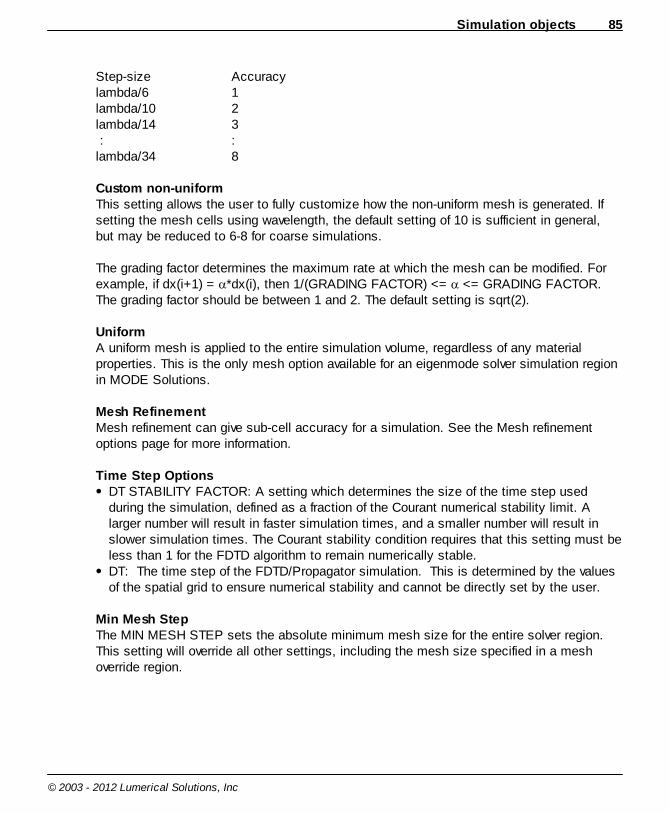
Simulation objects 85
© 2003 - 2012 Lumerical Solutions, Inc
Step-size Accuracylambda/6 1lambda/10 2lambda/14 3 : :lambda/34 8
Custom non-uniformThis setting allows the user to fully customize how the non-uniform mesh is generated. Ifsetting the mesh cells using wavelength, the default setting of 10 is sufficient in general,but may be reduced to 6-8 for coarse simulations.
The grading factor determines the maximum rate at which the mesh can be modified. Forexample, if dx(i+1) = *dx(i), then 1/(GRADING FACTOR) <= <= GRADING FACTOR.The grading factor should be between 1 and 2. The default setting is sqrt(2).
UniformA uniform mesh is applied to the entire simulation volume, regardless of any materialproperties. This is the only mesh option available for an eigenmode solver simulation regionin MODE Solutions.
Mesh RefinementMesh refinement can give sub-cell accuracy for a simulation. See the Mesh refinementoptions page for more information.
Time Step OptionsDT STABILITY FACTOR: A setting which determines the size of the time step usedduring the simulation, defined as a fraction of the Courant numerical stability limit. Alarger number will result in faster simulation times, and a smaller number will result inslower simulation times. The Courant stability condition requires that this setting must beless than 1 for the FDTD algorithm to remain numerically stable.DT: The time step of the FDTD/Propagator simulation. This is determined by the valuesof the spatial grid to ensure numerical stability and cannot be directly set by the user.
Min Mesh StepThe MIN MESH STEP sets the absolute minimum mesh size for the entire solver region.This setting will override all other settings, including the mesh size specified in a meshoverride region.
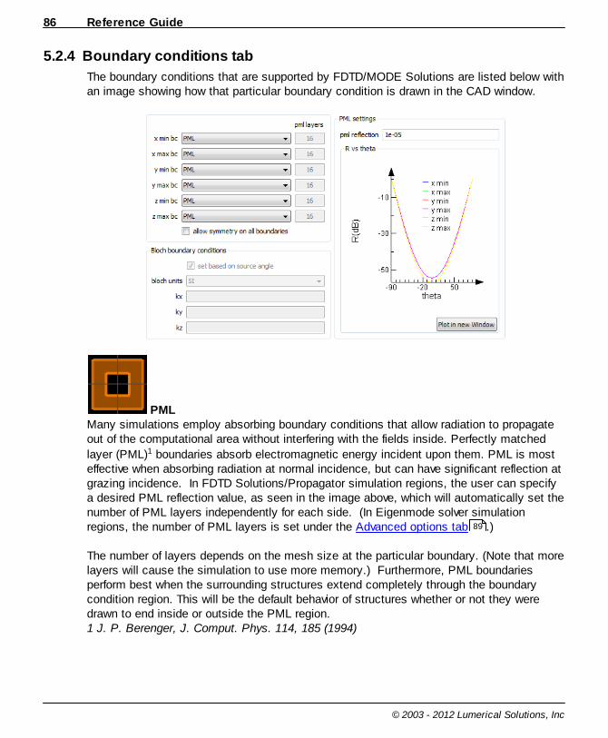
Reference Guide86
© 2003 - 2012 Lumerical Solutions, Inc
5.2.4 Boundary conditions tab
The boundary conditions that are supported by FDTD/MODE Solutions are listed below withan image showing how that particular boundary condition is drawn in the CAD window.
PMLMany simulations employ absorbing boundary conditions that allow radiation to propagateout of the computational area without interfering with the fields inside. Perfectly matched
layer (PML)1 boundaries absorb electromagnetic energy incident upon them. PML is mosteffective when absorbing radiation at normal incidence, but can have significant reflection atgrazing incidence. In FDTD Solutions/Propagator simulation regions, the user can specifya desired PML reflection value, as seen in the image above, which will automatically set thenumber of PML layers independently for each side. (In Eigenmode solver simulationregions, the number of PML layers is set under the Advanced options tab .)
The number of layers depends on the mesh size at the particular boundary. (Note that morelayers will cause the simulation to use more memory.) Furthermore, PML boundariesperform best when the surrounding structures extend completely through the boundarycondition region. This will be the default behavior of structures whether or not they weredrawn to end inside or outside the PML region.1 J. P. Berenger, J. Comput. Phys. 114, 185 (1994)
89
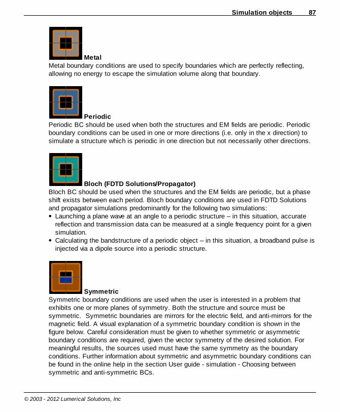
Simulation objects 87
© 2003 - 2012 Lumerical Solutions, Inc
MetalMetal boundary conditions are used to specify boundaries which are perfectly reflecting,allowing no energy to escape the simulation volume along that boundary.
PeriodicPeriodic BC should be used when both the structures and EM fields are periodic. Periodicboundary conditions can be used in one or more directions (i.e. only in the x direction) tosimulate a structure which is periodic in one direction but not necessarily other directions.
Bloch (FDTD Solutions/Propagator)Bloch BC should be used when the structures and the EM fields are periodic, but a phaseshift exists between each period. Bloch boundary conditions are used in FDTD Solutionsand propagator simulations predominantly for the following two simulations:
Launching a plane wave at an angle to a periodic structure – in this situation, accuratereflection and transmission data can be measured at a single frequency point for a givensimulation. Calculating the bandstructure of a periodic object – in this situation, a broadband pulse isinjected via a dipole source into a periodic structure.
SymmetricSymmetric boundary conditions are used when the user is interested in a problem thatexhibits one or more planes of symmetry. Both the structure and source must besymmetric. Symmetric boundaries are mirrors for the electric field, and anti-mirrors for themagnetic field. A visual explanation of a symmetric boundary condition is shown in thefigure below. Careful consideration must be given to whether symmetric or asymmetricboundary conditions are required, given the vector symmetry of the desired solution. Formeaningful results, the sources used must have the same symmetry as the boundaryconditions. Further information about symmetric and asymmetric boundary conditions canbe found in the online help in the section User guide - simulation - Choosing betweensymmetric and anti-symmetric BCs.
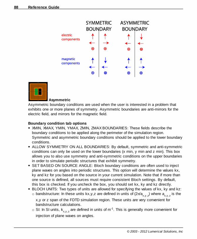
Reference Guide88
© 2003 - 2012 Lumerical Solutions, Inc
AsymmetricAsymmetric boundary conditions are used when the user is interested in a problem thatexhibits one or more planes of symmetry. Asymmetric boundaries are anti-mirrors for theelectric field, and mirrors for the magnetic field.
Boundary condition tab optionsXMIN, XMAX, YMIN, YMAX, ZMIN, ZMAX BOUNDARIES: These fields describe theboundary conditions to be applied along the perimeter of the simulation region.Symmetric and asymmetric boundary conditions should be applied to the lower boundaryconditions.ALLOW SYMMETRY ON ALL BOUNDARIES: By default, symmetric and anti-symmetricconditions can only be used on the lower boundaries (x min, y min and z min). This boxallows you to also use symmetry and anti-symmetric conditions on the upper boundariesin order to simulate periodic structures that exhibit symmetry.SET BASED ON SOURCE ANGLE: Bloch boundary conditions are often used to injectplane waves on angles into periodic structures. This option will determine the values kx,ky and kz for you based on the source in your current simulation. Note that if more thanone source is defined, all sources must require consistent Bloch settings. By default,this box is checked. If you uncheck the box, you should set kx, ky and kz directly. BLOCH UNITS: Two types of units are allowed for specifying the values of kx, ky and kz: o bandstructure: In these units kx,y,z are defined in units of (2 /a
x,y ,z) where a
x,y ,z is the
x,y or z span of the FDTD simulation region. These units are very convenient forbandstructure calculations.
o SI: In SI units, kx,y ,z
are defined in units of m-1. This is generally more convenient for
injection of plane waves on angles.

Simulation objects 89
© 2003 - 2012 Lumerical Solutions, Inc
KX, KY, KZ: The wavevector setting in the x, y and z direction for the Bloch boundary inthe units specified above.
5.2.5 Advanced options tab
WARNING: This tab includes options which should only be changed if you are quitefamiliar with the meshing algorithm and techniques used .
FDTD Solutions and MODE Solutions Propagator:
FORCE SYMMETRIC X, Y, Z MESH: This will force a symmetric mesh about the x, y or zaxis. When this option is enabled, the meshing algorithm ONLY considers objects in thepositive half of the simulation region. The mesh in the negative half is simply a copy of thepositive half mesh. All physical structures and mesh override regions in the negative halfwill not be considered by the meshing algorithm. This option also forces a mesh point atthe center of the simulation region. Forcing a symmetric mesh ensures that the meshdoes not change when going from a simulation with symmetry to a simulation withoutsymmetry. OVERRIDE SIMULATION BANDWIDTH FOR MESH GENERATION: This option allows thesimulation mesh to be generated following a custom wavelength or frequency range. Bydefault, the mesh is generated based on the source properties.SNAP PEC TO YEE CELL BOUNDARY: This option forces any structures defined as PECto have interfaces that are aligned with the Yee cell boundaries. This ensures that allelectric field components at the PEC interface are tangential to the interface. This settingavoids complications that can result in some circumstances if normal electric fieldcomponents are set to 0 at a PEC interface. To achieve this, the specified PEC interfacemay be shifted by as much as dx/2 when creating the simulation mesh, where dx is thesize of the Yee cell. For more information, please contact [email protected] USE COMPLEX FIELDS: This checkbox forces the algorithm to use complexfields during simulation. This will result in slower simulation times and increased memoryrequirements and should only be used when necessary. Without this, complex fields areonly used when there are Bloch boundary conditions. USE EARLY SHUTOFF: This will automatically end the simulation when most of theenergy has left the simulation volume. AUTO SHUTOFF MIN: The simulation will end when the total energy in the simulationvolume drops to this fraction of the maximum energy injected. The simulation data willautomatically save.USE DIVERGENCE CHECKING: This will automatically end the simulation when the totalenergy in the simulation volume is this many times larger than maximum energy injected. AUTO SHUTOFF MAX: The simulation will end when the total energy in the simulationvolume rises to this many times the maximum energy injected. The simulation data willautomatically save.DOWN SAMPLE TIME: Check the auto shutoff conditions every down sample time number

Reference Guide90
© 2003 - 2012 Lumerical Solutions, Inc
of dT time stepsPML KAPPA: The normalized imaginary electric and magnetic conductivity used in thePML boundaries. PML SIGMA: The maximum normalized electric and magnetic conductivity used in thePML boundaries. MINIMUM PML LAYERS: The minimum number of cells which are used for PML boundaryconditions. Increasing PML layers will reduce the back-reflection arising from theboundaries but will also increase time and memory requirements for simulations. Defaultsto a setting of 12. MAXIMUM PML LAYERS: The maximum number of cells which are used for PML boundaryconditions. Increasing PML layers will reduce the back-reflection arising from theboundaries but will also increase time and memory requirements for simulations. Defaultsto a setting of 64. PML POLYNOMIAL: The polynomial power which determines how rapidly the electric andmagnetic conductivity increases as radiation propagates at normal incidence into the PML.The default setting of 3 denotes a cubic increase of electric and magnetic conductivity withincreasing depth into the PML. TYPE OF PML: The type of PML used can be STANDARD or STABILIZED. In some cases,STABILIZED PML provides more numerical stability, although the performance is slightlyreduced.EXTEND STRUCTURE THROUGH PML: In most cases, we want the structures to extendthrough the PML so that fields exiting the simulation region are completely absorbed,otherwise there could be some unwanted back reflection. This option automaticallyextends structures through the region even if they were not drawn as such in the CAD.MAX SOURCE TIME SIGNAL LENGTH: This is the maximum length of data used bysources to store the “time” and “time_signal” properties of sources. If a large number ofsources are used and the simulation time is on the order of 100ps (which is very rare),advanced users may want to reduce this to save memory. However, since the “time” and“time_signal” properties of sources are important for calculating the sourcepower,sourcenorm, and the normalization for the transmission functions, care must be taken withsource normalization. In particular, in most cases, nonorm option should be used.SET PROCESS GRID: The division of of the simulation volume into sub-regions, which arethen run as a separate processes, can be manually set for more efficient computation. Better performance will be achieved when the regions are square e.g. for 20 regions, 5x2x2is more efficient than 20x1x1. NX, NY, NZ: The process layout for parallel simulations.SET DEFAULTS: Can be used to reset the settings back to their original default settings.
Simulation objects 91
© 2003 - 2012 Lumerical Solutions, Inc
5.3 SourcesThe following types of sources are available in FDTD Solutions and MODE Solutions'Propagator:
Point sources (dipole)Oscillating dipoles act as sources in Maxwell's equation to produce electromagnetic fields.Their position and direction are specified in terms of the center position (x, y, and z for 3Dsimulations) and their orientation through angles phi (measured in the x-y plane withrespect to the x-axis) and theta (measured from the z-axis). They can be placed at one ormore points anywhere in the simulation area.
For two-dimensional simulations, the behavior of point sources depends on whether you areperforming a TE or a TM simulation. For a TE simulation, a magnetic dipole is oriented inthe z-direction, while an electric dipole is oriented in the x-y plane by the ANGLEargument, which specifies the angle measured with respect to the x-axis. For a TMsimulation, an electric dipole is oriented in the z-direction, while a magnetic dipole isoriented in the x-y plane with the same ANGLE argument describing the direction of thedipole vector.
Gaussian and thin lens sourcesA Gaussian source defines a beam of electromagnetic radiation propagating in a specificdirection, with the amplitude defined by a Gaussian cross-section of a given width. Bydefault, the Gaussian sources use a scalar beam approximation for the electric field whichis valid as long as the waist beam diameter is much larger than the diffraction limit. Thescalar approximation assumes that the the fields in the direction of propagation are zero. For a highly focused beam, there is also a thin lens source that will inject a fully vectorialbeam. The cross section of this beam will be a Gaussian if the lens is not filled, and will bea sinc function if the lens is filled. In each case, the beams are injected along a lineperpendicular to the propagation direction, and are clipped at the edges of the source.
Note: References for the thin lens sourceThe field profiles generated by the thin lens source are described in the followingreferences. For uniform illumination (filled lens), the field distribution is precisely thesame as in the papers. For non-uniform illumination at very high NA (numerical aperture),there are some subtle differences. This is due to a slightly different interpretation ofwhether the incident beam is a Gaussian in real space or in k-space. This difference israrely of any practical importance because other factors such as the non-ideal lensproperties become important at these very high NA systems.
M. Mansuripur, "Distribution of light at and near the focus of high-numerical-aperture

Reference Guide92
© 2003 - 2012 Lumerical Solutions, Inc
objectives," J. Opt. Soc. Am. A 3,2086-2093 (1986). M. Mansuripur, "Certain computational aspects of vector diffraction problems," J. Opt.Soc. Am. A 6, 786-805 (1989). M. Mansuripur, "Distribution of light at and near the focus of high-numerical-apertureobjectives: erratum, Certain computational aspects of vector diffraction problems:erratum" J. Opt. Soc. Am. A 10, 382-383 (1993).
Plane wave sourcesPlane wave sources are used to inject laterally-uniform electromagnetic energy from oneside of the source region. In two-dimensional simulations, the plane wave source injectsalong a line, while in three-dimensional simulations the plane wave source injects along aplane. It is also possible to inject a plane wave at an angle. The plane wave source isactually the same object as the Gaussian source, with the only difference being theSOURCE SHAPE setting.
Total-field scattered-field sources Total-field scattered-field sources are used to separate the computation region into twodistinct regions – one contains the total field (i.e. the sum of the incident field and thescattered field), while the second region contains only the scattered field. The incident fieldis a plane wave with a wavevector normal to injection surface. This source type isparticularly useful to study the scattering behavior of objects, as the scattered field can beisolated from the incident field.
In 2D, the TFSF source injects along one edge of a rectangle as specified by the user. Theother three boundaries subtract the incident field (allowing for the wave propagation). Everything inside the TFSF boundary is total field (i.e. incident + scattered field), whileeverything outside is only scattered field. In the absence of any objects, the wavepropagates within the TFSF region and is subtracted out at the other end; this, of course,results in there being no scattered field. However, if one places an object in the path of theTFSF wave, this introduces scattered fields that then propagate outside of the total fieldarea. Consequently, one can then measure the total or scattered transmission, by placingmonitors inside or outside the total field region, respectively. Currently, only normalincidence plane waves are supported as the source field.
TIP: Using TFSF sourcesTFSF sources can be used when:
the source can completely surround the scattering objects in a homogeneous material(including materials with complex index).the scattering object is on or in a multilayer slab that is illuminated from above.
Certain boundaries of the TFSF can be dragged outside the simulation area boundaries,
Simulation objects 93
© 2003 - 2012 Lumerical Solutions, Inc
for example, when symmetric or anti-symmetric boundary conditions are used in thesimulation. For advanced use of TFSF sources, please consult an application example ortechnical support at [email protected].
Some care is needed when using the TFSF source. The concept of total/scattered field iscomplex and can lead to misinterpretation of results, particularly with regards to energyconservation.
Mode sourcesThe mode source is used to inject a guided mode into the simulation region. The geometryof the mode source (i.e. center location, and span) is used to compute the guided modesfor the structure. In three-dimensional simulations, the modes are computed across aplane, while in two-dimensions they are computed across a line. From a list of possiblemodes, a single mode is selected for injection into the simulation region. For additionaldetails on the operation of the mode solver, consult the integrated mode source section.
Import sources (FDTD Solutions only)The import source allows the user to specify a custom field profile for the source injectionplane. The custom field profile can be calculated from an analytic formula, imported fromanother FDTD simulation, or imported from other simulation tools such as Breault ResearchOrganization’s ASAP ray tracer. Imported sources are only available in 3D FDTDsimulations.
Global source optionsThe global source options window adjusts default frequency-domain parameters. Thesesettings can be used by any of the frequency domain sources by unchecking the 'overrideglobal source settings' checkbox in the source's Frequency/Wavelength tab.
5.3.1 General tab
The information located on the general tab depends on the type of monitor chosen. Notethat the POLARIZATION option is disabled for propagator simulations, where the actualpolarization of the source is determined in the propagator simulation region, under theeffective index tab. Otherwise, sources in propagator simulations are the same as sourcesin FDTD Solutions.
Dipole sourcesDIPOLE TYPE: A pull-down menu in which the point source can be configured as anelectric dipole or a magnetic dipole.
100

Reference Guide94
© 2003 - 2012 Lumerical Solutions, Inc
AMPLITUDE: The amplitude of the point source. The units of the source depend on thedipole type, as explained in the Units and normalization section. BASE AMPLITUDE: This is the amplitude that will generate a radiated CW power of 10nW/m in 2D simulations and 1 fW in 3D simulations. TOTAL AMPLITUDE: This is the amplitude actually used in the simulations, it is theproduct of the AMPLITUDE and the BASE AMPLITUDE. PHASE: The phase of the point source, measured in units of degrees. Only useful forsetting relative phase delays between multiple radiation sources. THETA: The angle with respect to the z axis of the dipole vectorPHI: Angle with respect to positive x axis of the dipole vector.
Gaussian, plane wave and TFSF sources(Some of the options below are not available for the TFSF source.)
SOURCE SHAPE: The shape of the beam. This setting defaults to Gaussian, but forconvenience can be changed to that of a Cauchy/Lorentzian, or a plane wave. AMPLITUDE: The amplitude of the source as explained in the Units and normalizationsection.PHASE: The phase of the point source, measured in units of degrees. Only useful forsetting relative phase delays between multiple radiation sources. INJECTION AXIS: Sets the axis along which the radiation propagates. DIRECTION: This field specifies the direction in which the radiation propagates.FORWARD corresponds to propagation in the positive direction, while BACKWARDcorresponds to propagation in the negative direction.ANGLE THETA: The angle of propagation, measured in degrees, with respect to theinjection axis defined above. ANGLE PHI: The angle of propagation, in degrees, rotated about the injection axis in aright-hand context.POLARIZATION ANGLE: The polarization angle defines the orientation of the injectedelectric field, and is measured with respect to the plane formed by the direction ofpropagation and the normal to the injection plane. A polarization angle of zero degreesdefines P-polarized radiation, regardless of direction of propagation while a polarizationangle of 90 degrees defines S-polarized radiation. THETA VS WAVELENGTH PLOT: This plot shows the actual injection angle theta foreach source wavelength as used in the simulation.
Mode and imported sources(Note that imported sources are only supported in FDTD Solutions.)
INJECTION AXIS: Sets the axis along which the mode source will propagate. DIRECTION: This field specifies the direction in which the TFSF source propagates.FORWARD corresponds to propagation in the positive direction, while BACKWARDcorresponds to propagation in the negative direction.AMPLITUDE: The amplitude of the mode source as explained in the Units andnormalization section.
37
37
37
Simulation objects 95
© 2003 - 2012 Lumerical Solutions, Inc
PHASE: The phase of the point source, measured in units of degrees. Only useful forsetting relative phase delays between multiple radiation sources. SELECT MODE: Mode source only. Launches the mode solver and allows the user toselect the desired mode for injection. For more information on using the mode source,consult the integrated mode solver section of the reference guide.THETA: The angle of propagation, measured in degrees, with respect to the injection axisdefined above. PHI: The angle of propagation, in degrees, rotated about the injection axis in a right-handcontext.OFFSET: Allows users to set an offset to the plane where the mode is calculated. This isuseful for ensuring that mode sources at an angle do not intersect with structures thatare not part of the waveguide/fiber.CLEAR SOURCE DATA: Clears the selected mode for mode sources, or clears theimported data for imported sourcesPLOT: This menu allows you to choose which component of the field profile you wouldlike to plot. PLOT CURRENT MODE/FIELD: This button will plot the field profile selected in the PLOTpull down menu for the currently selected mode.PLOT IN NEW WINDOW: This is the same as PLOT CURRENT MODE/FIELD but opensa new window for the graphics that stays open even after property edit window is closed.
Also for imported sources the following Imported source settings are availableX0, Y0, Z0: Displays the location in the imported source where the field was recorded. IMPORTED INDEX: The refractive index of the background medium where the importedfield was recorded. IMPORTED POWER: The power of the source recorded in imported. IMPORTED WAVELENGTH: The wavelength of the imported source data. IMPORT SOURCE: load an interface file (*.fld).
5.3.2 Geometry tab
The geometry tab contains options to change the size and location of the sources.
5.3.3 Frequency/Wavelength tab
The Frequency/Wavelength tab is shown below. This tab can be accessed through theindividual source properties, or the global source properties. Note that the plots on theright-hand side of the window update as the parameters are updated, so that you can easilyobserve the wavelength (top figure), frequency (middle figure) and temporal (bottom figure)content of the source settings.
100

Reference Guide96
© 2003 - 2012 Lumerical Solutions, Inc
At the top-left of the tab, it is possible to chose to either SET FREQUENCY /WAVELENGTH or SET TIME-DOMAIN. If you choose to set the frequency or wavelengthranges to define your sources, then FDTD Solutions/Propagator tries to find the optimumtime domain settings that will cover the desired frequency/wavelength range withoutcompromising accuracy. If you choose to directly modify the time domain settings, pleasekeep the following points in mind:
Pulse durations: Choose a pulse duration that can accurately span your frequency orwavelength range of interest. However, very short pulses contain many frequencycomponents and therefore disperse quickly. As a result, short pulses require more pointsper wavelength for accurate simulation. Pulse offset: This parameter defines the temporal separation between the start of thesimulation and the center of the input pulse. To ensure that the input pulse is nottruncated, the pulse offset should be at least 2 times the pulse duration. This will ensurethat the frequency distribution around the center frequency of the source is close tosymmetrical, and the initial fields are close to zero at the beginning of the simulation. Source type: In general, you can choose between ‘standard’ and ‘broadband’ sourcetypes. Standard sources consist of a Gaussian pulse at a fixed optical carrier, while thebroadband sources consist of a Gaussian pulse with an optical carrier which variesacross the pulse envelope. Broadband sources can be used to perform simulations inwhich wideband frequency data is required – for instance, from 200 to 1000 THz. Thistype of frequency range cannot be accurately simulated using the standard source type.
Simulation objects 97
© 2003 - 2012 Lumerical Solutions, Inc
Set frequency wavelengthIf the SET FREQUENCY / WAVELENGTH option was chosen, this section makes itpossible to either set the frequency or the wavelength and choose to either set the centerand span or the minimum and maximum frequencies of the source.
Set time domainThe options in the time domain section are:
SOURCE TYPE: This setting is used to specify whether the source is a standard sourceor a broadband source. The standard source consists of an optical carrier with a fixedfrequency and a Gaussian envelope. The broadband source, which contains a muchwider spectrum, consists of a chirped optical carrier with a Gaussian envelope. When theuser uses the script function setsourcesignal, this field will be set as "user input".FREQUENCY: The center frequency of the optical carrier. PULSELENGTH: The full-width at half-maximum (FWHM) power temporal duration of thepulse. OFFSET: The time at which the source reaches its peak amplitude, measured relative tothe start of the simulation. An offset of N seconds corresponds to a source whichreaches its peak amplitude N seconds after the start of the simulation. BANDWIDTH: The FWHM frequency width of the time-domain pulse.
AdvancedELIMINATE DISCONTINUITY: Ensures the function has a continuous derivative (smoothtransitions from/to zero) at the start and end of a user defined source time signal. Bydefault, this option is enabled.
5.3.4 Beam options tab
This tab is only available for Gaussian sources. In the general tab, set the source shapeoption to the desired shape (Gaussian, plane wave or Cauchy/Lorentzian) before enteringdata in the beam options tab because the beam options that are available will changedepending on the source shape.
Beam options for all source shapesCURRENT INDEX: This field shows the refractive index at the x,y (and z) position of thebeam. BEAM PROFILE, PLOT: This menu allows you to choose which component of the fieldprofile you would like to plot. SHOW/REFRESH: This button will update the current plot and the current index. Theplot is not automatically updated because the thin lens calculations can be long. PLOT IN NEW WINDOW: This is the same as SHOW/REFRESH but opens a newwindow for the graphics that will persist after you close the property edit window.
Beam options for Gaussian and Cauchy/Lorentizian sources USE SCALAR APPROXIMATION / USE THIN LENS: These checkboxes allow the user to

Reference Guide98
© 2003 - 2012 Lumerical Solutions, Inc
choose whether to use the scalar approximation for the electric field or the thin lenscalculation. Gaussian sources can be defined using either the scalar approximation or thinlens calculation, whereas Cauchy/Lorentzian sources can only be defined using the scalarapproximation.
Scalar approximationBEAM PARAMETERS: This menu is used to choose to define the scalar beam by theWAIST SIZE AND POSITION or the BEAM SIZE AND DIVERGENCE ANGLE. If WAIST SIZE AND POSITION is chosen, the options are:
WAIST RADIUS: 1/e field (1/e2 power) radius of the beam for a Gaussian beam, or a half-width half-maximum (HWHM) for the Cauchy/Lorentzian beam. DISTANCE FROM WAIST: The distance, d, as shown in the figure below. A positivedistance corresponds to a diverging beam, and a negative sign corresponds to aconverging beam.
If BEAM SIZE AND DIVERGENCE ANGLE is chosen, the options are:
BEAM RADIUS: 1/e field (1/e2 power) radius of the beam for a Gaussian beam, or a half-width half-maximum (HWHM) for the Cauchy/Lorentzian beam. DIVERGENCE ANGLE: Angle of the radiation spread as measured in the far field, asshown in the figure below. A positive angle corresponds to a diverging beam and anegative angle corresponds to a converging beam.
Thin LensReferences for the thin lens approximation are listed on the Sources page.
NA: This is nsin( ) where n is the refractive index of the medium in which the source isfound and is the half angle as shown in the figure below. Please note that the index willnot be correctly defined in dispersive media and lenses should only be used in non-dispersive media. The refractive index for the source is determined at X, Y (and Z). DISTANCE FROM FOCUS: The distance d from focus as shown in the figure below. Anegative distance indicates a converging beam and a positive distance indicates adiverging beam. FILL LENS: Checking this box indicates that the lens is illuminated with a plane wavewhich is clipped at the lens edge. If FILL LENS is unchecked, then it is possible to setthe diameter of the thin lens (LENS DIAMETER) and the beam diameter prior to strikingthe lens (BEAM DIAMETER), as shown in the figure below. A beam diameter muchlarger than the lens diameter is equivalent to a filled lens. NUMBER OF PLANE WAVES: This is the number of plane waves used to construct thebeam. The beam profile is more accurate as this number increases but the calculationtakes longer. The default value in 2D is 1000.
The figure below shows the beam parameter definitions for the scalar approximation beam.
91

Simulation objects 99
© 2003 - 2012 Lumerical Solutions, Inc
The figure below shows the beam parameter definitions for the thin lens, fully-vectorialbeam.
TIP: Setting Gaussian source parametersGaussian spot size: The beam spot sizecan be set independently of the sourcespan. The source span should be chosento be larger than the beam spot size. Ifthere is significant intensity at the edges ofthe source, as shown in this figure, thebeam will scatter on injection. If the spot size is larger than the simulationregion, the beam profile will be truncated atthe simulation boundary.
5.3.5 Advanced tab
This tab only appears for the dipole source. The tab contains a RECORD LOCAL FIELDcheckbox. When checked, the fields around the dipole are saved; this box must bechecked in order to use the dipolepower script function.
Reference Guide100
© 2003 - 2012 Lumerical Solutions, Inc
5.3.6 Integrated mode source
This section describes the operation of the integrated mode solver to inject guided wavesinto FDTD simulations or the Propagator in MODE Solutions. The mode solver itself usesthe same discretization mesh as the FDTD/propagator algorithm, so the profile of theguided modes as computed with the mode solver naturally interface with the underlyingFDTD/propagator mesh. Overall, this facilitates the injection of guided modes with minimalback-reflection.
This section describes the operation of the integrated mode solver once the physicalstructure and the simulation region defining the structure of interest have been definedwithin the layout editor. The mode source is launched by pressing the SELECT MODEbutton within the mode source edit window. Following this, the mode source windowappears with different tabs. The following sections detail each tab within the mode solverwindow, and the information which it contains.
5.3.6.1 Mode analysis
The MODE ANALYSIS window is shown in the screenshot below. The upper portion of thewindow contains the MODE LIST where the mode number, effective index, propagationloss, and polarization (percentage of the mode polarized TE; not valid for 3D simulations)are shown. The lower left-hand corner shows the calculation parameters; upon launch, thelower left-hand portion of the window shows the default calculation parameters to be usedto simulate the structure. The right-hand portion of the window contains the PLOT AREAwhere the simulation data is plotted, and the two drop-down boxes at the top of the plotarea are used to specify which data to plot in the plot window, while the region at thebottom right can be used to modify the current mode plot options. Upon launch, the plotarea shows the refractive index profile of the structure being analyzed.

Simulation objects 101
© 2003 - 2012 Lumerical Solutions, Inc
Modal analysisThe modal analysis portion of the window displays simulation data relevant to the differentmodes calculated for the structure of interest. This portion of the window shows the modes,arranged from top to bottom in terms of the highest effective index and numberedsequentially. For each mode, this portion of the window shows the effective index of themode, the calculated loss (measured in dB per millimeter of propagation; only valid forlossy materials), and the TE or TM fraction corresponding to the definition of TE and TM in2D FDTD. For 3D FDTD simulations, the TE or TM fraction is not displayed. Note that thereare small differences between FDTD Solutions and the Propagator in MODE Solutions,please see Mode List and Deck page in the MODE Solutions Knowledge Base for the lattercase.
See the following section for more information about the analysis and plot sections.
Select ModePressing this button (located on the lower right corner of the window) will initialize the modesource with the current mode selected within the mode table in the upper left-hand portionof the window.
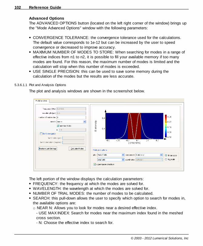
Reference Guide102
© 2003 - 2012 Lumerical Solutions, Inc
Advanced OptionsThe ADVANCED OPTIONS button (located on the left right corner of the window) brings upthe "Mode Advanced Options" window with the following parameters:
CONVERGENCE TOLERANCE: the convergence tolerance used for the calculations.The default value corresponds to 1e-12 but can be increased by the user to speedconvergence or decreased to improve accuracy. MAXIMUM NUMBER OF MODES TO STORE: When searching for modes in a range ofeffective indices from n1 to n2, it is possible to fill your available memory if too manymodes are found. For this reason, the maximum number of modes is limited and thecalculation will stop when this number of modes is exceeded. USE SINGLE PRECISION: this can be used to save some memory during thecalculation of the modes but the results are less accurate.
5.3.6.1.1 Plot and Analysis Options
The plot and analysis windows are shown in the screenshot below.
The left portion of the window displays the calculation parameters:FREQUENCY: the frequency at which the modes are solved for. WAVELENGTH: the wavelength at which the modes are solved for.NUMBER OF TRIAL MODES: the number of modes to be calculated. SEARCH: this pull-down allows the user to specify which option to search for modes in,the available options are:o NEAR N: Allows you to look for modes near a desired effective index.
- USE MAX INDEX: Search for modes near the maximum index found in the meshedcross section. - N: Choose the effective index to search for.

Simulation objects 103
© 2003 - 2012 Lumerical Solutions, Inc
o IN RANGE: Allows you to search for modes in a desired range of indices.
- N1, N2: Define the range of indices to search over. BENT WAVEGUIDE: Allows the user to specify a current radius of curvature for themode and solver for the modes of a bent waveguide. o BEND RADIUS: the bend radius of the waveguide measured from the center of the
mode solver regiono BEND ORIENTATION: the orientation of the radius of curvature.
CALCULATE MODE: by clicking this button the mode solver will start the calculation forthe waveguide modes given the criteria above.RESTORE LAST SETTINGS: restores the calculation parameters to the currentsimulation parameters corresponding to the modes that have been calculated.
Figure windowThe plot itself where the data appears is automatically labeled and scaled to fit thesimulation data. As with the layout editor, the plot can be zoomed using the standardmouse actions. Note, however, that the mouse is automatically in the zoom state whenover the plotted data and therefore the keyboard shortcut Z is not necessary.
Mode plot optionsThe MODE PLOT OPTIONS can be set in the bottom right of the MODE ANALYSISwindow, the options are
PLOT: This pull-down allows the user specifies what simulation data should be plottedwithin the plot area.
Box 1 specifies what general class of data to plot: o MODAL FIELDS: allows the user to select various field quantities such as electric and
magnetic field amplitudes and intensities and Poynting vectors using theCOMPONENT pull-down
o MATERIAL PROPERTIES: allows the user to select various physical quantities such
as refractive index, permittivity, and conductivity using the COMPONENT pull-down Box 2 specifies which part of complex-valued simulation data is to plot:o AMPLITUDE
o PHASE
o REAL PART
o IMAGINARY PART
COMPONENT: This pull-down allows the user to specify which specific component is tobe plotted within the plot area. The available options depend on the setting of the PLOTpull-down. COORDINATES: currently supports only the CARTESIAN coordinate system. LINEAR/LOG SCALE: determines whether the simulation data is plotted on a linear or alog plot SUPERIMPOSE STRUCTURE: toggles whether a black outline showing the physicalstructure is superimposed on the simulation data
Reference Guide104
© 2003 - 2012 Lumerical Solutions, Inc
5.4 MonitorsThe following types of monitors are available in FDTD Solutions and MODE Solutions'Propagator:
Index monitorsIndex monitors records the n and k value as a function of frequency/wavelength in asimulation. Index monitors are only available in two or three dimensions; there is no optionfor linear or point index monitors. In the future, the index monitor will be able to capture thetime-evolution of the physical properties profile for nonlinear media.
Time-domain monitorsThese monitors provide time-domain information for field components over the course of thesimulation. Time-domain monitors can consist of point, line, or area monitors to capturethis information over different spatial extents within the FDTD simulation region. For thepurposes of extracting line widths of resonant structures through Fourier analysis, pointtime monitors with a down sample time of 1 are sufficient.
TIP: Using time monitorsCheck the memory requirements when using 1D, 2D or 3D time monitors, since they willgenerate large amounts of data. Consider using the temporal or spatial down-samplingoptions.
Movie monitorsMovie monitors capture a desired field component over the region spanned by the monitorfor the duration of the simulation. Movie monitors are only available in the two dimensionalvariety (and only z-normal for propagator simulations). The resultant movies are saved withthe same name as the monitor in the current working directory.
TIP: CW MoviesIt is possible to create a CW movie from profile or power monitor data. For moreinformation, see the User Guide - Data Analysis section of the online Knowledge Base.
Frequency-domain profile monitorsFrequency-domain profile monitors collect the field profile in the frequency domain fromsimulation results across some spatial region within the simulation. Individual fieldcomponents, Poynting vector, and power flow can be collected as a function of frequencyand position. These monitors will record field profiles exactly where they are positioned.

Simulation objects 105
© 2003 - 2012 Lumerical Solutions, Inc
Profile monitors are ideally used to collect field data for visualization and customizedanalysis. If highly accurate power measurements are required, power monitors should beused, rather than profile monitors.
Tip: Using frequency monitors Beware that frequency-domain field-profile monitors are computationally-intensive andthey can increase the simulation time considerably. When possible, try to use 1D or 2Drather than than 3D monitors; if it is necessary to use the latter, try to restrict the numberof frequency points. We suggest experimenting with the spatial downsample value(s)before doing long simulations and watch how long your simulation takes. If you are onlyinterested in the power flux, you can select only OUTPUT POWER in the Data to recordtab.
Frequency-domain power monitorsFrequency-domain power monitors collect high-accuracy power flow information in thefrequency domain from simulation results across some spatial region within the simulation.These monitors are identical to Frequency-domain profile monitors except that theyautomatically snap to the nearest FDTD mesh cell boundary when the simulation runs dueto a different default setting of the SPATIAL INTERPOLATION property in the advancedoption. This is important when accurate power flow calculations are required. Lessinterpolation is required in this case, which results in slightly more accurate powermeasurements. Unfortunately, this also means that the exact position where the data isrecorded will change whenever the mesh changes. If it is more important to measure thefield at a particular position, profile monitors should be used.
The precise location of where the monitor measures data during the simulation is recordedwith the monitor data in the x, y and z vectors.
Tip: When to use profile and power monitorsProfile monitors: when it is most important to measure the fields at a very specific point inspace.Power monitors: when it is most important to get the most accurate powermeasurements.
TIP: Switching between power monitor and profile monitorYou can switch between frequency-domain power monitors and frequency-domain profilemonitors by changing the SPATIAL INTERPOLATION setting in the Advanced Optionstab. When the SPATIAL INTERPOLATION is set to NEAREST MESH CELL or NONE,the monitor becomes a frequency-domain power monitor.
Reference Guide106
© 2003 - 2012 Lumerical Solutions, Inc
Mode Expansion MonitorsMode Expansion Monitors use overlap analysis to calculate the forward/backwardpropagating components of any mode of a waveguide or fiber at an arbitrary location in thesimulation region. The Mode Expansion monitor facilitates the interoperability betweenFDTD Solutions and INTERCONNECT as it returns the S parameters, which can beimported into INTERCONNECT directly.
Global Monitor PropertiesThe global monitor options window is where the user can specify the range and resolutionwith which to measure frequency-domain information. These settings can be used by anyof the frequency domain monitors by unchecking the 'override global monitor settings'checkbox in the monitor's General tab.
5.4.1 Frequency Power/Profile tab
This tab only appears for the global monitor settings, but includes the same options as thegeneral tab does for frequency domain power and profile monitors.
USE LINEAR WAVELENGTH SPACING: By default, data is recorded at linearly spacedpoints with respect to frequency. Selecting this option spaces data at linearly spacedpoints with respect to wavelength.USE SOURCE LIMITS: When checked these monitors use the source limits. Whenunchecked, the frequencies/wavelengths at which to record data can be set using thepull down menus and boxes below them. FREQUENCY POINTS: Set to choose the number of frequency points at which to recorddata.
5.4.2 Frequency Power/Profile Advanced tab
This tab only appears for the global monitor settings. It contains advanced global settingsfor frequency-domain monitors. Only the MIN SAMPLING PER CYCLE can be modified bythe user.
MIN SAMPLING PER CYCLE: This parameter determines the minimum amount ofsampling per optical cycle that can be used. By default, it is set at 2 (the Nyquist limit)for optimum efficiency. DESIRED SAMPLING: This converts the minimum points per optical cycle into an actualsampling rate in Hz. NYQUIST LIMIT: The Nyquist sampling limit is calculated based on the maximumfrequencies that may be present in the simulation volume. ACTUAL SAMPLING: The actual sampling rate is the rate that will actually be used forthe discrete fourier transforms (DFTs), taking into account the desired sampling rate, theNyquist limit and the time step, dt.
Simulation objects 107
© 2003 - 2012 Lumerical Solutions, Inc
DOWN SAMPLE TIME: This is the time step downsampling.
5.4.3 General tab
The information located on the general tab depends on the type of monitor chosen. Thereare three different possibilities, which are outlined below.
Movie monitorHORIZONTAL RESOLUTION: The horizontal width of the final movie, in pixels.VERTICAL RESOLUTION: The vertical height of the final movie, in pixels.SCALE: A dimensionless variable which defines how to scale the capture of the fielddata, with the tendency that a scale factor too small will result in saturation of the movie,while a scale factor too large will result in very faint radiation patterns. This parametermay not be less than zero. Tip: for Gaussian pulses, this is best set to unity. For dipolesources, it is typically on the order of 0.01 to 0.05. The monitor outputs its maximumintensity at the end of the simulation in the variable Monitor Name_maxI. Setting thescale factor to Monitor Name_maxI and rerunning the simulation will result in a perfectlyscaled movie. DRAW STRUCTURE OUTLINE: A toggle which allows the user to superimpose anoutline of the refractive index profile on top of the movie. This can be used to aid invisualization of where the radiation is located within the dielectric structure. TM, TE FIELD COMPONENT: 2D simulations. The field component to be captured in themovie. The choices depend on whether a TE or TM simulation is being performed, as setout in the FDTD simulation region. If a TM simulation is being performed, the TM fieldcomponent is captured to the movie, whereas if a TE simulation is being performed, the
TE field component is captured. Can also be ELECTRIC FIELD INTENSITY (|E|2) or
MAGNETIC FIELD INTENSITY (|H|2).FIELD COMPONENT: 3D simulations. The field component to be captured in the movie.
Can also be ELECTRIC FIELD INTENSITY (|E|2) or MAGNETIC FIELD INTENSITY (|H|2).
Time-domain monitorThe general tab for the time domain monitor includes options to edit the amount of data,and time period over which data is collected.
Index, frequency domain profile and frequency domain power monitorsOVERRIDE GLOBAL MONITOR SETTINGS: A toggle to override the global monitorsettings. If checked, the user can specify the frequency range and number of points atwhich frequency-domain information will be recorded (using the options described below).If unchecked the options below are set from the global monitor settings.USE LINEAR WAVELENGTH SPACING: By default, data is recorded at linearly spacedpoints with respect to frequency. Selecting this option spaces data at linearly spacedpoints with respect to wavelength.USE SOURCE LIMITS: When checked these monitors use the source limits. Whenunchecked, the frequencies/wavelengths at which to record data can be set using the
Reference Guide108
© 2003 - 2012 Lumerical Solutions, Inc
pull down menus and boxes below them. FREQUENCY POINTS: Set to choose the number of frequency points at which to recorddata.
5.4.4 Data to record tab
STANDARD FOURIER TRANSFORM: The monitor outputs data at specific frequencies.PARTIAL SPECTRAL AVERAGE:The monitor outputs the partial spectral average powerthrough a monitor surface, normalized to the partial spectral average of the source.TOTAL SPECTRAL AVERAGE: The monitor outputs the total spectral average powerthrough a monitor surface, normalized to the total spectral average of the source.OUTPUT EX, EY, EZ, HX, HY, HZ, PX, PY, PZ: A set of fields with which the user canselect what field components (EX, EY, EZ, HX, HY, HZ) or Poynting vector (PX, PY, PZ)to measure. In 2D simulations, only some components are non-zero (i.e. only EX, EY,and HZ are applicable for TE simulations). All the field quantities remain active tofacilitate easy change between TE and TM simulations. OUTPUT POWER: For surface monitors (3D) and line monitors (2D) only. You cancalculate the integrated power over the monitor surface. This requires much less memoryafter the simulation is completed and is particularly suitable for large parallel simulationswhere only the integrated power across a surface is required.
5.4.5 Geometry tab
The geometry tab contains options to change the size and location of the monitors.
The DOWNSAMPLE X, Y, Z option is used to set the spatial averaging performed on thedata. A down sample value of N corresponds to averaging over N grid points. Setting thedown sample value to 1 gives the most detailed spatial information (i.e. information at eachgrid point).
5.4.6 Spectral averaging and apodization tab
PARTIAL SPECTRAL AVERAGING, DELTA: FWHM of the Lorentzian weightingfunction.APODIZATION: Specifies the window function of the apodization. Options include none,start (i.e. beginning of time signature apodized), end (i.e. end of time signature apodized,or full (i.e. both start and end). Note that apodization will, in general, invalidate anysource normalization performed and is therefore not suitable for accurate powermeasurements. APODIZATION CENTER, TIME WIDTH, FREQ WIDTH: See the diagram below for thedefinition of these terms. The FREQ WIDTH corresponds to the effective bandwidth of thefull apodization window, as described under APODIZATION.
Note: Apodization functions

Simulation objects 109
© 2003 - 2012 Lumerical Solutions, Inc
FULL apodization involves windowing the time-domain data on both the start and endside. The resulting “windowed” data is then processed to produce frequency-domaininformation. START apodization involves windowing the front side of the time-domain data. This can beuseful to exclude the initial source excitation from the frequency-domain data. END apodization involves windowing the last part of the simulation. This can be useful forramping down the time-domain signal in devices where the radiation lives a long time, likecavities.
5.4.7 Advanced tab
Time-domain monitorsSPATIAL INTERPOLATION: In FDTD generally, the electromagnetic field componentsare not recorded at the same point in space. Instead each component of the vectorialelectric and magnetic fields are recorded at different locations in the Yee cell. In order toproperly calculate the Poynting vector and electromagnetic energy density, the fields areinterpolated to the same location in the Yee cell. This setting controls how the fields areinterpolated. Currently, the supported options for time monitors are NEAREST MESHCELL and NONE. With NEAREST MESH CELL, the fields are interpolated to the nearestFDTD mesh cell boundary. With NONE, no interpolation is performed and eachelectromagnetic field component is recorded at a different position within the Yee cell.MIN SAMPLING PER CYCLE: This parameter determines the minimum amount ofsampling per optical cycle that can be used. By default, it is set at 10. SAMPLING RATE: The actual sampling rate in Hz. DOWN SAMPLE TIME: This is the time step downsampling.
Frequency domain profile and power monitorsSPATIAL INTERPOLATION: This option is as described above for time domain monitorsOVERRIDE ADVANCED GLOBAL MONITOR SETTINGS: When this option is selectedMIN SAMPLING PER CYCLE can be set. The other options cannot be altered, they arethere to display settings. For further details, see the descriptions in Frequency Power/Profile Advanced tab .
Movie monitorsMIN SAMPLING PER CYCLE: This parameter determines the desired amount of
106

Reference Guide110
© 2003 - 2012 Lumerical Solutions, Inc
sampling per optical cycle. SAMPLING RATE: This converts the minimum points per optical cycle into an actualsampling rate in Hz. DOWN SAMPLE TIME: This is the time step downsampling. FRAME RATE: The speed at which frames are displayed on the screen, in units offrames per second. The default is 30.
Index monitors:SPATIAL INTERPOLATION: There are three options for index monitors. The defaultoption, SPECIFIED POSITION returns the index that that the field sees at the locationwhere the monitor is placed. The next two options. NEAREST MESH CELL and NONEare as described for time-domain monitors. In simulations with mesh refinement turnedon, the default option does not show the averaging of the indices, but the other optionsdo.
5.4.8 Setup tab
The setup tab is only available for analysis groups. The setup tab contains two further tabs:the variables tab, and the script tab. The variables tab is identical to the properties tabfor structure groups and the script tab is identical to the script tab for structure groups.
For more information and examples, see the Analysis groups page of the User Guidesection of the Online Help.
5.4.9 Analysis tab
The analysis tab is only available for analysis groups. The analysis tab contains two furthertabs, the variables and the script tab. The variables tab is used to define the input andoutput parameters of the script, and the script command contains script that can be usedto process the monitor data.
Variables tabPARAMETERS: These are input parameters to the analysis script. RESULTS: The output parameters are defined here. The analysis script must calculatethese quantities. Once the analysis script has been run, the results become monitordata, that can be accessed using script commands in the same manner that monitordata is accessed for simple monitors.
Script tabThe script has access to the input parameters defined in the variables tab, and can getdata from any of the monitors located in the group. However, it cannot get data frommonitors or sources not located inside that group. The script in the analysis groups doesnot use the global variable space from the script prompt and script file editor. The resultsfrom the script can be obtained in the script prompt by setting up output parameters in thevariables tab.
82
82

Simulation objects 111
© 2003 - 2012 Lumerical Solutions, Inc
The following buttons and regions are available in the script tab:ANALYSIS SCRIPT: This is where the script commands are written. To find a list ofscript commands, see the Scripting Language section of the Reference Guide.ANALYSIS SCRIPT OUTPUT: Press the RUN ANALYSIS button to run the script. If thereare no syntax errors in the script the SCRIPT OUTPUT will read <script complete>.
In addition, the analysis script output will contain any results from the "?" scriptcommand.RUN ANALYSIS: Pressing the run analysis prompt runs the analysis script and savesthe results. This button can only be pressed when the simulation is in analysis mode.SAVE ANALYSIS: Pressing this button saves changed made to the analysis script (evenwhen in analysis mode).
For more information and examples, see the Analysis groups page of the User Guidesection of the Online Help.
155

Reference Guide112
© 2003 - 2012 Lumerical Solutions, Inc
5.4.10 Mode expansion tab
This tab only appears for the Mode Expansion monitors.
The Mode Expansion tab contains two main sections. The "Mode calculation" sectionallows users to select a mode (or a set of modes) to expand the monitor data with. The"Monitors for expansion" section allows users to choose a field profile from an arbitrarymonitor in the simulation to expand. For more information on this expansion calculation,and the results that are returned, see Overlap analysis.
Mode Calculation
MODE SELECTION: Allows users to select the modes to use for the mode expansioncalculation. The "user select" option allows users to select multiple modes.
Simulation objects 113
© 2003 - 2012 Lumerical Solutions, Inc
Following the "mode selection" combo box is a frame for choosing the frequencies tocalculate the modes for. Note that this does not have to correspond to the frequency pointsfor the monitors in the "Monitors for expansion" table. The mode expansion monitor willautomatically perform the necessary interpolation between different frequency points.
OVERRIDE GLOBAL MONITOR SETTINGS: A toggle to override the global monitorsettings. If checked, the user can specify the frequency range and number of points atwhich the modes will be calculated at (using the options described below). If unchecked,the options below are set from the global monitor settings.USE LINEAR WAVELENGTH SPACING: By default, modes are calculated at linearlyspaced points with respect to frequency. Selecting this option spaces the points withrespect to wavelength.USE SOURCE LIMITS: When checked these monitors use the source limits. Whenunchecked, the frequencies/wavelengths at which to record data can be set using thepull down menus and boxes below them. FREQUENCY POINTS: Set to choose the number of frequency points at which tocalculate the modes.
SELECT MODE: If the "user selected" option has been chosen, this will bring up the Mode analysis tab for the user select from a calculated list of modes.VISUALIZE MODE DATA: This will bring up the Visualizer, showing all the profiles for theselected modes. CLEAR MODE DATA: Clears all the mode data.
RotationsThis frame allows user to apply an arbitrary rotation to the calculate modes.
THETA: The angle of propagation, measured in degrees, with respect to the normal axis.PHI: The angle of propagation, in degrees, rotated about the normal axis in a right-handcontext.OFFSET: Allows users to set an offset to the plane where the modes are calculated.This is useful for ensuring that monitors at an angle do not intersect with unwantedstructures.
AdvancedAUTO UPDATE BEFORE ANALYSIS: If selected, the monitor will automatically updatethe chosen modes when necessary.
Monitors for expansion
After the modes have been selected, the next step is to choose the monitor with the inputfield profile. The "Add" and "Remove" buttons on the side can be used to add/removemonitors, and users can choose the desired monitor from the monitor drop down list.
100
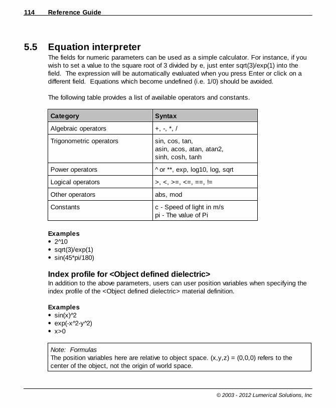
Reference Guide114
© 2003 - 2012 Lumerical Solutions, Inc
5.5 Equation interpreterThe fields for numeric parameters can be used as a simple calculator. For instance, if youwish to set a value to the square root of 3 divided by e, just enter sqrt(3)/exp(1) into thefield. The expression will be automatically evaluated when you press Enter or click on adifferent field. Equations which become undefined (i.e. 1/0) should be avoided.
The following table provides a list of available operators and constants.
Category Syntax
Algebraic operators +, -, *, /
Trigonometric operators sin, cos, tan, asin, acos, atan, atan2,sinh, cosh, tanh
Power operators or **, exp, log10, log, sqrt
Logical operators >, <, >=, <=, ==, !=
Other operators abs, mod
Constants c - Speed of light in m/spi - The value of Pi
Examples2 10sqrt(3)/exp(1)sin(45*pi/180)
Index profile for <Object defined dielectric>In addition to the above parameters, users can user position variables when specifying theindex profile of the <Object defined dielectric> material definition.
Examplessin(x) 2 exp(-x 2-y 2)x>0
Note: FormulasThe position variables here are relative to object space. (x,y,z) = (0,0,0) refers to thecenter of the object, not the origin of world space.
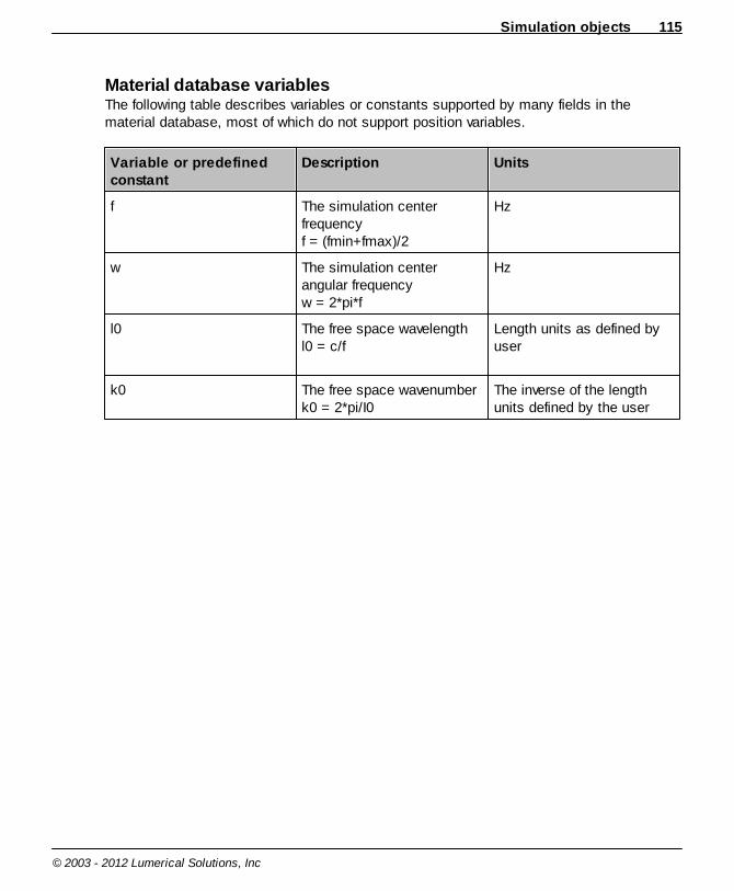
Simulation objects 115
© 2003 - 2012 Lumerical Solutions, Inc
Material database variablesThe following table describes variables or constants supported by many fields in thematerial database, most of which do not support position variables.
Variable or predefinedconstant
Description Units
f The simulation centerfrequency f = (fmin+fmax)/2
Hz
w The simulation centerangular frequencyw = 2*pi*f
Hz
l0 The free space wavelengthl0 = c/f
Length units as defined byuser
k0 The free space wavenumberk0 = 2*pi/I0
The inverse of the lengthunits defined by the user
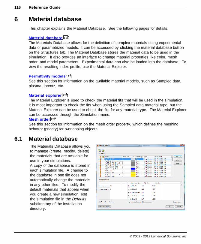
Reference Guide116
© 2003 - 2012 Lumerical Solutions, Inc
6 Material database
This chapter explains the Material Database. See the following pages for details.
Material databaseThe Materials Database allows for the definition of complex materials using experimentaldata or parametrized models. It can be accessed by clicking the material database buttonon the Structures tab. The Material Database stores the material data to be used in thesimulation. It also provides an interface to change material properties like color, meshorder, and model parameters. Experimental data can also be loaded into the database. Toview the resulting index profile, use the Material Explorer.
Permittivity modelsSee this section for information on the available material models, such as Sampled data,plasma, lorentz, etc.
Material explorerThe Material Explorer is used to check the material fits that will be used in the simulation. It is most important to check the fits when using the Sampled data material type, but theMaterial Explorer can be used to check the fits for any material type. The Material Explorercan be accessed through the Simulation menu. Mesh orderSee this section for information on the mesh order property, which defines the meshingbehavior (priority) for overlapping objects.
6.1 Material databaseThe Materials Database allows youto manage (create, modify, delete)the materials that are available foruse in your simulations. A copy of the database is stored ineach simulation file. A change tothe database in one file does notautomatically change the materialsin any other files. To modify thedefault materials that appear whenyou create a new simulation, editthe simulation file in the Defaultssubdirectory of the installationdirectory.
116
117
125
127

Material database 117
© 2003 - 2012 Lumerical Solutions, Inc
Import / ExportThe import and export buttons allow you to transfer material data between simulation filesvia Material Database Files (.mdf) files.
Material list The material list shows the materials stored in the material database. A number ofmaterials are provide with the product installation. To create additional materials, use theAdd button. You can also modify some of the material properties (name, color, meshorder, etc) in the list view.
Default materials provided with the product installation are write protected, and can not bedirectly modified. To modify the properties of a default material, simply use the Copybutton to duplicate the material. The copy will be unlocked. The first column of the listshows which materials are write protected.Materials currently used in the simulation can not be deleted. The second column of thelist shows which materials are in use. To delete these materials, first modify the simulationso they are not used.
Material PropertiesUse the Material properties window to view and edit the material model parameters. Formodel parameter definitions, see the material models section.
6.2 Permittivity modelsThis section describes the permittivity (or refractive index) material models supported bythe Material Database. Model parameters can be edited in the Material property panel ofthe Material Database window.
Sampled dataThe Sampled data model is used to import experimental material data. The experimentaldata can be imported from a text file with the Import data button.
The Sampled data material definition uses an automatic fitting routine to generate a multi-coefficient material model of the experimental data over the frequency range specified bythe source.The fitting routine can use one of the models described below, or a moregeneralized model. The fits can be checked and adjusted in the Material Explorer.
Tolerance - The desired RMS error between the permittivity of the experimental data andthe material fit. The fitting routine will use the least number of coefficients that produce a fitwith an RMS error less than the tolerance. Max coefficients - The maximum number of coefficients allowed to be used in the materialfit. More coefficients can produce a more accurate fit, but will make the simulation slower.

Reference Guide118
© 2003 - 2012 Lumerical Solutions, Inc
The following advanced options can be set in the Material Explorer:
Make Fit Passive - Set to be true to prevent the fit from having gain at any frequency. Bydefault this is true in order to prevent diverging simulations.Improve Stability - If this setting is true, the fitting routine restricts the range of coefficientsin the fit in order to reduce numerical instabilities which cause simulations to diverge.Imaginary Weight - Increasing the weight increases the importance of the imaginary part ofthe permittivity when calculating a fit. A weight of 1 gives equal weight to the imaginary andreal parts of the permittivity.Specify Fit Range - Set to true to decouple the bandwidth used to generate the material fitand the source bandwidth. This option is used in parameter sweeps where the sourcefrequency is changed, and where it is important to keep the material parameters constantover the whole parameter sweep. The fit range should cover the simulation bandwidth.Bandwidth range - Bandwidth to be used for the fit when Specify Fit Range is true.
DielectricThe Dielectric model is used to create a material with a constant real index. This materialwill have the specified index at all frequencies (non-dispersive).
Refractive index - The refractive index of the material. Must be >= 1.
(n,k) materialThe (n,k) material model is used to create a material with a specific value of n and k at asingle frequency.
Refractive index - Real part of the index at the center frequency of the simulation. Must be> 0. Imaginary refractive index - Imaginary part of the index at the center frequency of thesimulation. Positive values correspond to loss, negative values will produce gain.
NOTE: Single frequency simulations only!This type of material model should only be used for single frequency simulations. Theimplementation of the (n,k) material model is such that the material properties will only becorrect at the center frequency of the simulation.
ConductiveThe Conductive model is used to create a material defined by the following formula.
o
totalf
if2
)(
Plasma (drude)
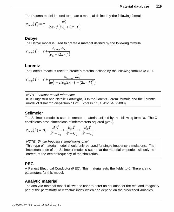
Material database 119
© 2003 - 2012 Lumerical Solutions, Inc
The Plasma model is used to create a material defined by the following formula.
fiff
C
Ptotal
22)(
2
DebyeThe Debye model is used to create a material defined by the following formula.
fif
C
Cdebye
total2
)(
LorentzThe Lorentz model is used to create a material defined by the following formula ( > 1).
22
2
)2(22)(
ffif
OO
Olorentztotal
NOTE: Lorentz model reference:Kurt Oughstun and Natalie Cartwright, "On the Lorentz-Lorenz formula and the Lorentzmodel of dielectric dispersion," Opt. Express 11, 1541-1546 (2003)
SellmeierThe Sellmeier model is used to create a material defined by the following formula. The Ccoefficients have dimensions of micrometers squared ( m2).
32
23
22
22
12
21
1)(C
B
C
B
C
BAtotal
NOTE: Single frequency simulations only!This type of material model should only be used for single frequency simulations. Theimplementation of the Sellmeier model is such that the material properties will only becorrect at the center frequency of the simulation.
PECA Perfect Electrical Conductor (PEC). This material sets the fields to 0. There are noparameters for this model.
Analytic materialThe analytic material model allows the user to enter an equation for the real and imaginarypart of the permittivity or refractive index which can depend on the predefined variables

Reference Guide120
© 2003 - 2012 Lumerical Solutions, Inc
listed below.
The predefined variables that can be used in the equations for "real" and "imaginary" are:- f: the frequency in the specified frequency units- l0: the free space wavelength in the specified length units- w: 2*pi*f in the specified units- k0: 2*pi/l0 where l0 is in the specified length units- pi: the number pi- c: the speed of light in a vacuum, ALWAYS in SI units, ie, always equal to 3e8- x1,...,x10: numeric values that represent a parameter of interest
Kerr nonlinearIn the Kerr nonlinear model, the electric polarization field P will depend on the electric fieldE in the following manner.
)(|)(|)( 2)3()1(0 tEtEtP
Solving for the displacement field D gives
tEtEtD r (|)(|)( 2)3(0
The relative permittivity and
)3(
values must be specified by the user.
Chi2
This nonlinear model allow users to define the value for the
)2(
term directly. An arbitrarydispersive base material can also be specified, in which case the added polarization will be
in addition to the polarization of any base material that is selected. If the )1(
term is 0(default), the polarization will be added to the vacuum.
Chi3/Chi2The usage for the Chi3/Chi2 material is the same as the Chi2 material, but with the additionof the Chi3 term.
Note that higher orders terms can also be modeled via the User-defined models .
ParamagneticThe paramagnetic material model allows the user to specify both the permittivity andpermeability of the material to simulate magnetic materials.
122
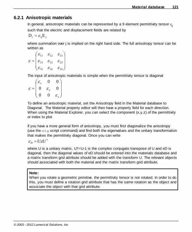
Material database 121
© 2003 - 2012 Lumerical Solutions, Inc
6.2.1 Anisotropic materials
In general, anisotropic materials can be represented by a 9 element permittivity tensor ij
such that the electric and displacement fields are related by
jiji ED
where summation over j is implied on the right hand side. The full anisotropy tensor can bewritten as
333231
232221
131211
The input of anisotropic materials is simple when the permittivity tensor is diagonal
z
y
x
00
00
00
To define an anisotropic material, set the Anisotropy field in the Material database toDiagonal. The Material property editor will then have a property field for each direction. When using the Material Explorer, you can select the component (x,y,z) of the permittivityor index to plot.
If you have a more general form of anisotropy, you must first diagonalize the anisotropy(use the eig script command) and find both the eigenvalues and the unitary transformation
that makes the permittivity diagonal. Once you can write†UUD
where U is a unitary matrix, U†=U-1 is the complex conjugate transpose of U and eD isdiagonal, then the diagonal values of eD should be entered into the materials database anda matrix transform grid attribute should be added with the transform U. The relevant objectsshould associated with both the material and the matrix transform grid attribute.
Note:When you rotate a geometric primitive, the permittivity tensor is not rotated. In order to dothis, you must define a rotation grid attribute that has the same rotation as the object andassociate the object with that grid attribute.
Reference Guide122
© 2003 - 2012 Lumerical Solutions, Inc
6.3 User-defined modelsUsers can define their own plugin material models written in C++. These material modelscan be compiled as a plugin and added to the materials database.
Basic concept
To create a new material, you must write a method in C++ that solves the following
equation for for En
nnnn VPEU
where En is the electric field at time n t, Pn is the desired polarization at time n t and Un
and Vn are input values that we provide. The polarization that is added will be in addition tothe polarization of any base material that is selected. If no base material is selected, thepolarization will be added to the vacuum (ie. the default relative permittivity or permeabilityis 1.)
The same approach is used to create new magnetic materials.
Simple example
Suppose you want to implement a simple linear, non-dispersive polarization that is addedto Lumerical's default multi-coeffiient model (MCM) for Silicon from Palik. The polarizationthat we want to add is simply
EP
In FDTD, this means that for each component of E in this material, you want to have nn EP
and therefore you need to solvennnn VEEU
for En by implementing a method that returns
n
nn
U
VE
Once this material plugin has been created, you simply add this material to the databaseand select Silicon as the base material. You will now have a material with a totalpermittivity of
)()( MCM
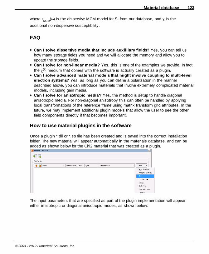
Material database 123
© 2003 - 2012 Lumerical Solutions, Inc
where MCM
( ) is the dispersive MCM model for Si from our database, and is the
additional non-dispersive susceptibility.
FAQ
Can I solve dispersive media that include auxilliary fields? Yes, you can tell ushow many storage fields you need and we will allocate the memory and allow you toupdate the storage fields.Can I solve for non-linear media? Yes, this is one of the examples we provide. In fact
the (2) medium that comes with the software is actually created as a plugin.Can I solve advanced material models that might involve coupling to multi-levelelectron systems? Yes, as long as you can define a polarization in the mannerdescribed above, you can introduce materials that involve extremely complicated materialmodels, including gain media.Can I solve for anisotropic media? Yes, the method is setup to handle diagonalanisotropic media. For non-diagonal anisotropy this can often be handled by applyinglocal transformations of the reference frame using matrix transform grid attributes. In thefuture, we may implement additional plugin models that allow the user to see the otherfield components directly if that becomes important.
How to use material plugins in the software
Once a plugin *.dll or *.so file has been created and is saved into the correct installationfolder. The new material will appear automatically in the materials database, and can beadded as shown below for the Chi2 material that was created as a plugin.
The input parameters that are specified as part of the plugin implementation will appeareither in isotropic or diagonal anisotropic modes, as shown below:
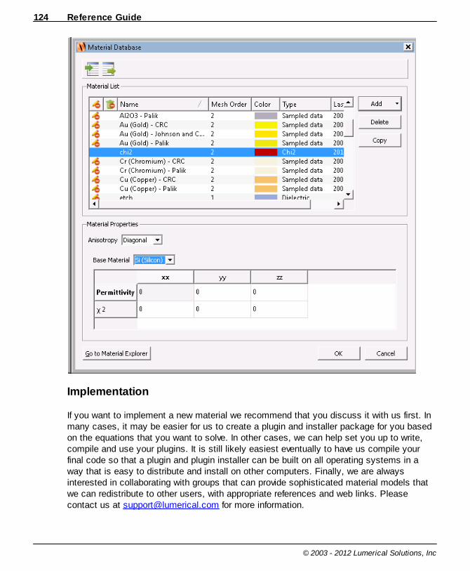
Reference Guide124
© 2003 - 2012 Lumerical Solutions, Inc
Implementation
If you want to implement a new material we recommend that you discuss it with us first. Inmany cases, it may be easier for us to create a plugin and installer package for you basedon the equations that you want to solve. In other cases, we can help set you up to write,compile and use your plugins. It is still likely easiest eventually to have us compile yourfinal code so that a plugin and plugin installer can be built on all operating systems in away that is easy to distribute and install on other computers. Finally, we are alwaysinterested in collaborating with groups that can provide sophisticated material models thatwe can redistribute to other users, with appropriate references and web links. Pleasecontact us at [email protected] for more information.
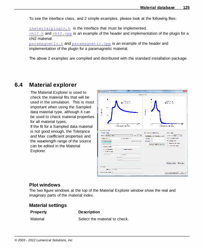
Material database 125
© 2003 - 2012 Lumerical Solutions, Inc
To see the interface class, and 2 simple examples, please look at the following files:
imaterialplugin.h is the interface that must be implemented.
chi2.h and chi2.cpp is an example of the header and implementation of the plugin for a
chi2 material.paramagnetic.h and paramagnetic.cpp is an example of the header and
implementation of the plugin for a paramagnetic material.
The above 2 examples are compiled and distributed with the standard installation package.
6.4 Material explorerThe Material Explorer is used tocheck the material fits that will beused in the simulation. This is mostimportant when using the Sampleddata material type, although it canbe used to check material propertiesfor all material types.If the fit for a Sampled data materialis not good enough, the Toleranceand Max coefficient properties andthe wavelength range of the sourcecan be edited in the MaterialExplorer.
Plot windowsThe two figure windows at the top of the Material Explorer window show the real andimaginary parts of the material index.
Material settings
Property Description
Material Select the material to check.
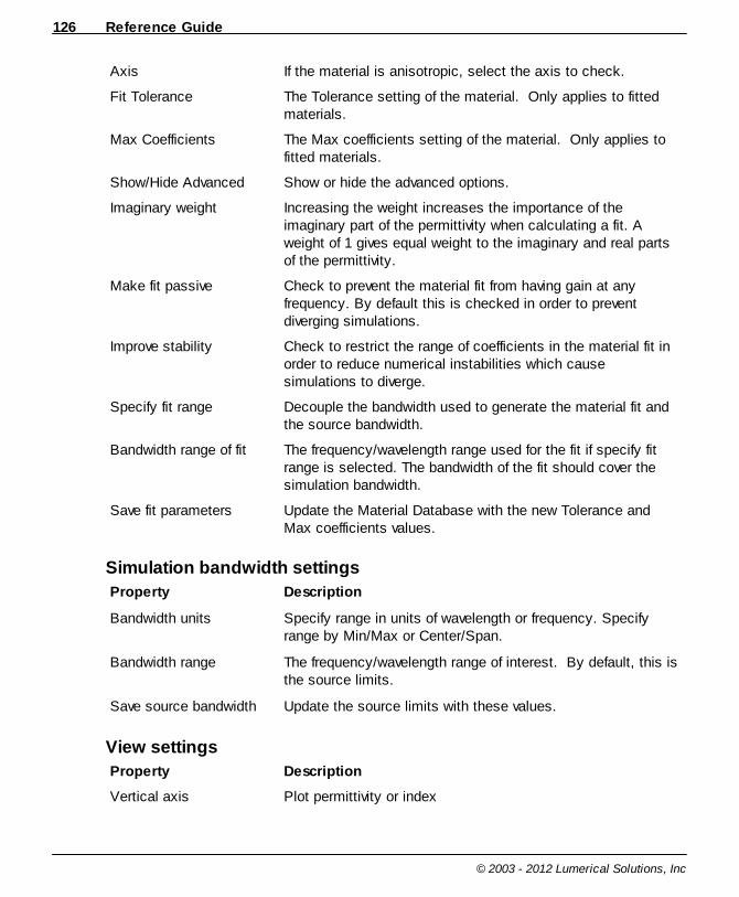
Reference Guide126
© 2003 - 2012 Lumerical Solutions, Inc
Axis If the material is anisotropic, select the axis to check.
Fit Tolerance The Tolerance setting of the material. Only applies to fittedmaterials.
Max Coefficients The Max coefficients setting of the material. Only applies tofitted materials.
Show/Hide Advanced Show or hide the advanced options.
Imaginary weight Increasing the weight increases the importance of theimaginary part of the permittivity when calculating a fit. Aweight of 1 gives equal weight to the imaginary and real partsof the permittivity.
Make fit passive Check to prevent the material fit from having gain at anyfrequency. By default this is checked in order to preventdiverging simulations.
Improve stability Check to restrict the range of coefficients in the material fit inorder to reduce numerical instabilities which causesimulations to diverge.
Specify fit range Decouple the bandwidth used to generate the material fit andthe source bandwidth.
Bandwidth range of fit The frequency/wavelength range used for the fit if specify fitrange is selected. The bandwidth of the fit should cover thesimulation bandwidth.
Save fit parameters Update the Material Database with the new Tolerance andMax coefficients values.
Simulation bandwidth settings
Property Description
Bandwidth units Specify range in units of wavelength or frequency. Specifyrange by Min/Max or Center/Span.
Bandwidth range The frequency/wavelength range of interest. By default, this isthe source limits.
Save source bandwidth Update the source limits with these values.
View settings
Property Description
Vertical axis Plot permittivity or index

Material database 127
© 2003 - 2012 Lumerical Solutions, Inc
Show material data Show the experimental data on the plot windows
Standard view Plot the fit over the specified bandwidth range
Extended view range Plot the fit over a wider bandwidth range
Specify view range Specify the range to plot the fit
Plot in new window Plots fit and data in a new window
Fit and plot buttons
Property Description
Plot in new window Plot data in a new window
Fit and Plot Calculate and plot the material fit
Fit analysis
Property Description
RMS error The RMS error of the fit. The fitting algorithm will use theminimum number of coefficients required to achieve an RMSerror less than the value specified by the Tolerance property ofthat material.
Number of coefficients The number of coefficients used in the fit.
6.5 Mesh orderThe mesh order property governs how overlapping objects are meshed in the simulation. Itserves no role for objects which do not overlap. The mesh order can be set at the materiallevel (in the material database), or the object object level (in the object properties). Materials with a lower mesh order take priority over materials with a higher priority number(i.e. order 1 takes priority over 2). Areas which overlap are assigned the materialproperties of the higher priority material (see the following figure).
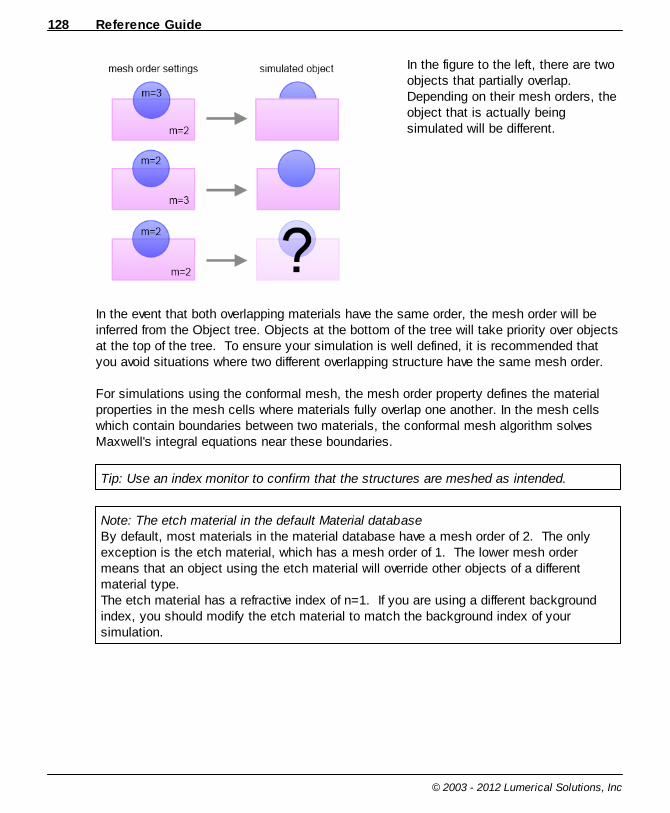
Reference Guide128
© 2003 - 2012 Lumerical Solutions, Inc
In the figure to the left, there are twoobjects that partially overlap. Depending on their mesh orders, theobject that is actually beingsimulated will be different.
In the event that both overlapping materials have the same order, the mesh order will beinferred from the Object tree. Objects at the bottom of the tree will take priority over objectsat the top of the tree. To ensure your simulation is well defined, it is recommended thatyou avoid situations where two different overlapping structure have the same mesh order.
For simulations using the conformal mesh, the mesh order property defines the materialproperties in the mesh cells where materials fully overlap one another. In the mesh cellswhich contain boundaries between two materials, the conformal mesh algorithm solvesMaxwell's integral equations near these boundaries.
Tip: Use an index monitor to confirm that the structures are meshed as intended.
Note: The etch material in the default Material databaseBy default, most materials in the material database have a mesh order of 2. The onlyexception is the etch material, which has a mesh order of 1. The lower mesh ordermeans that an object using the etch material will override other objects of a differentmaterial type. The etch material has a refractive index of n=1. If you are using a different backgroundindex, you should modify the etch material to match the background index of yoursimulation.
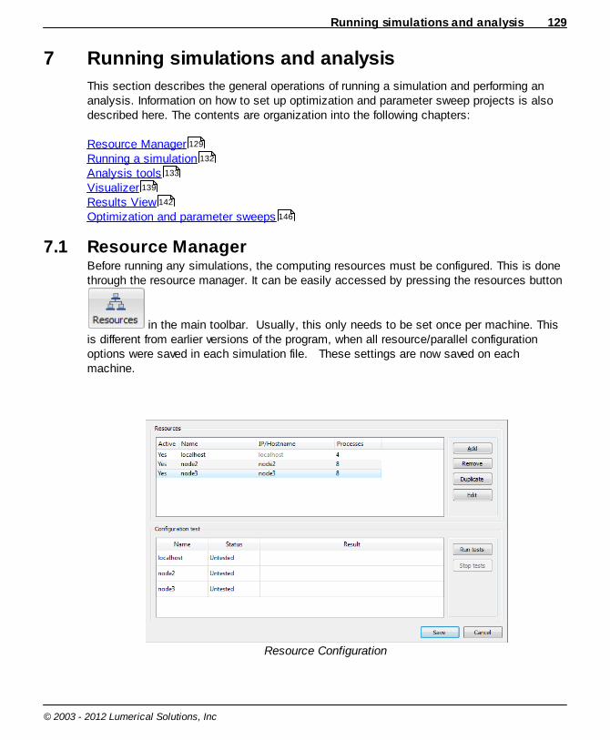
Running simulations and analysis 129
© 2003 - 2012 Lumerical Solutions, Inc
7 Running simulations and analysis
This section describes the general operations of running a simulation and performing ananalysis. Information on how to set up optimization and parameter sweep projects is alsodescribed here. The contents are organization into the following chapters:
Resource ManagerRunning a simulationAnalysis toolsVisualizerResults ViewOptimization and parameter sweeps
7.1 Resource ManagerBefore running any simulations, the computing resources must be configured. This is donethrough the resource manager. It can be easily accessed by pressing the resources button
in the main toolbar. Usually, this only needs to be set once per machine. Thisis different from earlier versions of the program, when all resource/parallel configurationoptions were saved in each simulation file. These settings are now saved on eachmachine.
Resource Configuration
129
132
133
139
142
146

Reference Guide130
© 2003 - 2012 Lumerical Solutions, Inc
USERS WITH A SINGLE LICENSEResourcesThis section allows the number of processes for localhost to be changed as well as thename. For advanced configuration options, see Resources Advanced Options .
Configuration testRun tests to make sure MPI username and password are set correctly. It also performsother checks such as engine path verification. If the tests pass, then we can be sure thatthe current simulation will run.
USERS WITH EXTRA ENGINE LICENSESResourcesIf you have extra engine licenses and Lumerical software installed on other computers onthe network, they can be added as additional computation resources to perform multiplesimulations in parallel. This is especially useful for parameter sweeps and optimizationprojects where many iterations need to be performed. The resources can easily be turnedon and off depending on whether they are free to compute at the time.
Requirements of each additional resource:Must be the same operating system as localhostMust be the same system type as localhost (cannot mix 32-bit with 64-bit)Must have the same version of Lumerical software as localhostMust have the same version of MPI as localhostMust have a user account with the same login and password as localhostMust have access to the simulation files via a network drive
To add a new resource:1. Click the add button.2. Set 'active' if you plan to use the resource right away or 'inactive' if you plan to enable it
later3. Set a name for that resource4. Specify the IP address of the hostname that the computer uses on the network5. Set the number of cores that you would like it to use6. Set any advanced options.
If many resources have advanced options that need to be changed, the 'Duplicate' buttonwill be useful.
Configuration testThis section of the window is used to test the communication to the additional resources. It runs a series of tests and will report any warnings or errors that may prevent a distributedsimulation from running such as mismatched software versions, user credentials orcommunication problems.
131
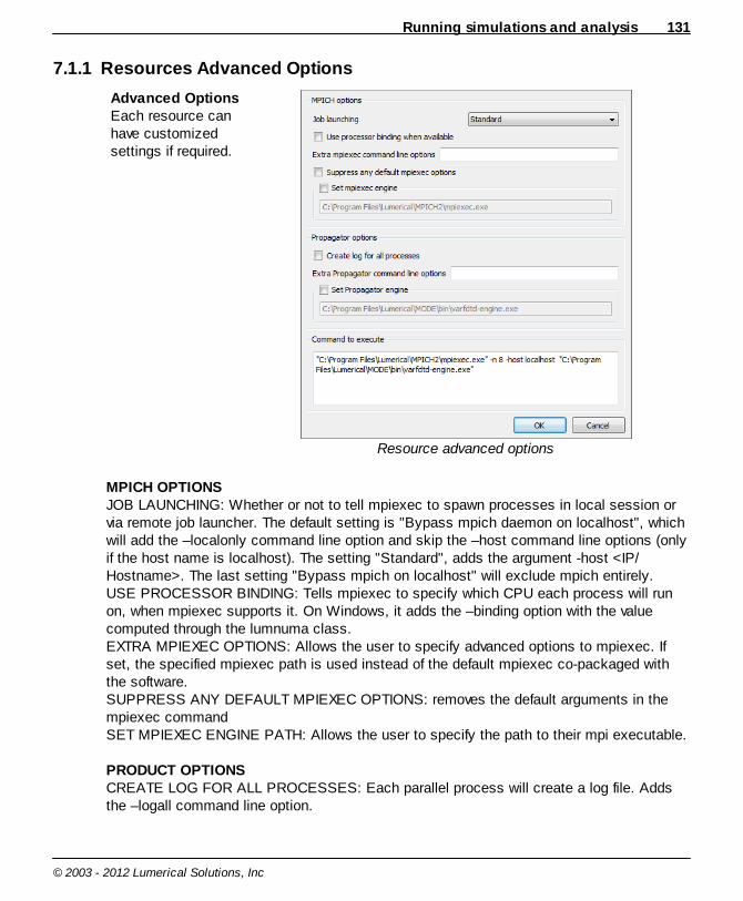
Running simulations and analysis 131
© 2003 - 2012 Lumerical Solutions, Inc
7.1.1 Resources Advanced Options
Advanced OptionsEach resource canhave customizedsettings if required.
Resource advanced options
MPICH OPTIONSJOB LAUNCHING: Whether or not to tell mpiexec to spawn processes in local session orvia remote job launcher. The default setting is "Bypass mpich daemon on localhost", whichwill add the –localonly command line option and skip the –host command line options (onlyif the host name is localhost). The setting "Standard", adds the argument -host <IP/Hostname>. The last setting "Bypass mpich on localhost" will exclude mpich entirely.USE PROCESSOR BINDING: Tells mpiexec to specify which CPU each process will runon, when mpiexec supports it. On Windows, it adds the –binding option with the valuecomputed through the lumnuma class.EXTRA MPIEXEC OPTIONS: Allows the user to specify advanced options to mpiexec. Ifset, the specified mpiexec path is used instead of the default mpiexec co-packaged withthe software.SUPPRESS ANY DEFAULT MPIEXEC OPTIONS: removes the default arguments in thempiexec commandSET MPIEXEC ENGINE PATH: Allows the user to specify the path to their mpi executable.
PRODUCT OPTIONSCREATE LOG FOR ALL PROCESSES: Each parallel process will create a log file. Addsthe –logall command line option.
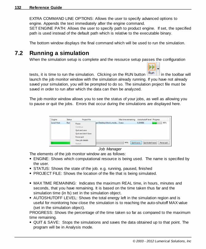
Reference Guide132
© 2003 - 2012 Lumerical Solutions, Inc
EXTRA COMMAND LINE OPTIONS: Allows the user to specify advanced options toengine. Appends the text immediately after the engine command.SET ENGINE PATH: Allows the user to specify path to product engine. If set, the specifiedpath is used instead of the default path which is relative to the executable binary.
The bottom window displays the final command which will be used to run the simulation.
7.2 Running a simulationWhen the simulation setup is complete and the resource setup passes the configuration
tests, it is time to run the simulation. Clicking on the RUN button in the toolbar willlaunch the job monitor window with the simulation already running. If you have not alreadysaved your simulation, you will be prompted to do so. The simulation project file must besaved in order to run after which the data can then be analyzed.
The job monitor window allows you to see the status of your jobs, as well as allowing youto pause or quit the jobs. Errors that occur during the simulations are displayed here.
Job ManagerThe elements of the job monitor window are as follows:
ENGINE: Shows which computational resource is being used. The name is specified bythe user.STATUS: Shows the state of the job. e.g. running, paused, finishedPROJECT FILE: Shows the location of the file that is being simulated.
MAX TIME REMAINING: Indicates the maximum REAL time, in hours, minutes andseconds, that you have remaining. It is based on the time taken thus far and thesimulation time (in fs) set in the simulation object. AUTOSHUTOFF LEVEL: Shows the total energy left in the simulation region and isuseful for monitoring how close the simulation is to reaching the auto-shutoff MAX value(set in the simulation object).
PROGRESS: Shows the percentage of the time taken so far as compared to the maximumtime remaining.
QUIT & SAVE: Stops the simulations and saves the data obtained up to that point. Theprogram will be in Analysis mode.
Running simulations and analysis 133
© 2003 - 2012 Lumerical Solutions, Inc
QUIT & DON'T SAVE: Stops the simulations and does not save any data. The programwill be in Layout mode.FORCE QUIT: Closes the job monitor window and forcefully terminates all simulations.This option should ONLY be used when the other Quit options don't work properly. When simulations are stopped with Force Quit, they may not check-in their license,which means you may have to wait several minutes before another simulation can be run. No simulation data will be saved.TOTAL PROGRESS BAR: The progress bar indicates how much of ALL the simulationsare complete, with the length of the progress bar is determined by the sum of the“maximum simulation times”.
To access actions for each job, right-clicking anywhere on the row will bring up a contextmenu with the following options:
PAUSE: the engine is signaled to go into a wait mode (it will stay running, but notconsume CPU)CONTINUE: restarts a paused jobQUIT AND SAVE: The engine will stop the current simulation job and attempt to save thedata created so far. QUIT AND DON'T SAVE: The engine will stop the current simulation job and does notsave any data.FORCE QUIT: Forcefully terminates the current simulation job and does not save anydata. This options should ONLY be used when other Quit options don't work properly.When simulations are stopped with Force Quit, they may not check-in their license,which means you may have to wait several minutes before another simulation can berun. VIEW JOB DETAILS: Opens up a modal dialog that contains the standard outputmessages from the engine processes.
Note: More informationFor more information about running Lumerical simulations, including running on clusters,using a job scheduler, preparing batch files, and using extra engine licenses, see theOnline Help section User Guide - Running Simulations.
7.3 Analysis toolsThis section describes the way in which the integrated analysis routines are used tovisualize and analyze simulation data. The manner in which the analysis routine interactswith the overall simulation environment is described in the next section: Analysis tools and the simulation environment . This is followed by sections tofamiliarize the user with the operation of the analysis routines.
The first section entitled Analysis groups describes the analysis tab of an analysisobject. In the second section, the two general ways in which data can be visualized and
134
134
Reference Guide134
© 2003 - 2012 Lumerical Solutions, Inc
analyzed is detailed. The plotting functions, a central component to the overall analysisroutines, are described in Figure windows section. The section entitled Data exportdescribes data can be exported to plot in other software packages for further analysis orformal presentation. Finally, the Visualizer and Results View tools are explained.Together, they provide a very useful and intuitive way of analyzing and visualizing resultsthrough the GUI. More advanced analysis can be performed with the extensive scriptinglanguage, as described in the Scripting language section.
7.3.1 Analysis tools and the simulation environment
Before describing how the analysis routines are used for data visualization, it is importantto understand the way in which the integrated analysis tool interacts with the simulationenvironment. Following the completion of a simulation, the simulation data is written intothe simulation project file; even premature termination of a simulation results in a partialdataset being written to the file. When the simulation completes and the EXIT button ispressed, or the simulation is prematurely terminated by pressing the EXIT button, theproject file will be in Analysis mode, meaning that any modification of the data will requireswitching back to the layout mode.
In Analysis mode, simulation object properties can be viewed, but not edited. This ensuresthat at any given time, the simulation data results corresponds to the configuration of thesimulation project. Once in the analysis tool, the user continues to analyze the simulationdata until they either wish to close the application, or they decide they would like to alterthe simulation objects and re-perform the simulation. By exiting the analysis routines andreturning to the layout editor, existing simulation data will be erased.
7.3.2 Analysis groups
Analysis groups are container objects that can contain any simulation object andassociated script functions which can be used to create customize data analysis. Forexample, an absorption monitor group can be created with a power monitor, an indexmonitor, and the script function that calculates absorption from these objects. One canalso automate an optimization/parameter sweep procedure using an analysis group madeof structures/simulation regions/sources/monitors, and use the script function to updateeach parameter accordingly.
An example of the edit window for an analysis group is shown in the screenshot below.
136 138
139 142
155

Running simulations and analysis 135
© 2003 - 2012 Lumerical Solutions, Inc
As can be seen above, there is a SETUP tab and an ANALYSIS tab. The SETUP tabcontains all the information needed to edit and set up monitors that are located in theanalysis group. The functionality of the SETUP tab is very similar to the Structure groupsobject. It is only possible to edit information in the SETUP tab in layout mode, butinformation in the SCRIPT tab can be edited both in layout and analysis mode (see thenote at the top of the window which is highlighted in yellow).
The ANALYSIS tab contains all the information used to analyze the monitor data. It isdivided into two sub-tabs. The VARIABLES tab contains all input parameters in the top half,and the output parameters (named results) in the bottom half. Parameters can be addedand removed using the respective buttons. Any changes to the variables can be savedusing the SAVE ANALYSIS button at the bottom of the tab. The RUN ANALYSIS buttonruns the analysis script located in the SCRIPT tab.
Once an analysis routine has run, the results (output parameters) become monitor data,which can be accessed from the script prompt or a script file in the same manner thatmonitor data is accessed for simple monitors.
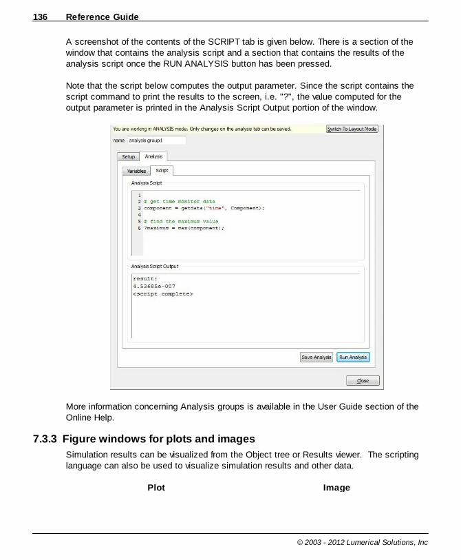
Reference Guide136
© 2003 - 2012 Lumerical Solutions, Inc
A screenshot of the contents of the SCRIPT tab is given below. There is a section of thewindow that contains the analysis script and a section that contains the results of theanalysis script once the RUN ANALYSIS button has been pressed.
Note that the script below computes the output parameter. Since the script contains thescript command to print the results to the screen, i.e. "?", the value computed for theoutput parameter is printed in the Analysis Script Output portion of the window.
More information concerning Analysis groups is available in the User Guide section of theOnline Help.
7.3.3 Figure windows for plots and images
Simulation results can be visualized from the Object tree or Results viewer. The scriptinglanguage can also be used to visualize simulation results and other data.
Plot Image
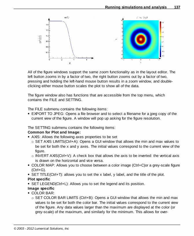
Running simulations and analysis 137
© 2003 - 2012 Lumerical Solutions, Inc
All of the figure windows support the same zoom functionality as in the layout editor. Theleft button zooms in by a factor of two, the right button zooms out by a factor of two,pressing and holding the left-hand mouse button results in a zoom window, and double-clicking either mouse button scales the plot to show all of the data.
The figure window also has functions that are accessible from the top menu, whichcontains the FILE and SETTING.
The FILE submenu contains the following items:EXPORT TO JPEG: Opens a file browser and to select a filename for a jpeg copy of thecurrent view of the figure. A window will pop up asking for the figure resolution.
The SETTING submenu contains the following items:Common for Plot and Image:
AXIS: Allows the following axes properties to be seto SET AXIS LIMITS(Ctrl+A): Opens a GUI window that allows the min and max values to
be set for both the x and y axes. The initial values correspond to the current view of thefigure.
o INVERT AXIS(Ctrl+V): A check box that allows the axis to be inverted: the vertical axis
is drawn on the horizontal and vice versa.COLOR MAP: Allows you to choose between a color image (Ctrl+C)or a grey-scale figure(Ctrl+G).SET TITLE(Ctrl+T): allows you to set the x label, y label, and the title of the plot.
Plot specificSET LEGEND(Ctrl+L): Allows you to set the legend and its position.
Image specificCOLOR BAR:o SET COLOR BAR LIMITS (Ctrl+B): Opens a GUI window that allows the min and max
values to be set for both the color bar. The initial values correspond to the current viewof the figure. Any data values larger than the maximum are displayed at the color (orgrey-scale) of the maximum, and similarly for the minimum. This allows for over-
Reference Guide138
© 2003 - 2012 Lumerical Solutions, Inc
saturation of the colors to emphasize certain regions of the image, or for moreaccurate comparison between two images.
o RESET DEFAULT LIMITS(Ctrl+D): Resets the original limits. This corresponds to the
minimum and maximum values of the data being imaged.
7.3.4 Data export
In some cases, the user may wish to export the simulation data to take advantage of theadvanced plotting and data analysis tools not available in Lumerical's products. Data exportcan be done in a number of ways, but in general the use of the scripting language will berequired. The user can use scripting commands as described in the Scripting languagesection to write data into text format, or alternatively use Matlab by directly calling Matlabfunctions in Lumerical or by exporting data to .mat files.
Export to text filesThe data subset export facility in the analysis view allows the user to save to a specifiedfilename, a subset of the total simulation data for quick plotting in other software packages.For x-y plots, the data subset export facility generates a two-column ASCII data file, with aheader which specifies where the data was taken from and the column headings with units.For image plots, the data subset consists of two columns which specify the x and ypositions in the units specified within the CAD layout editor, and a matrix of data whichconsists of the field quantities being exported. The user may also write a script file andutilize the write script function to custom create a text file.
MatlabMATLAB has a number of specialized plotting functions useful for visualizing simulationdata. For example, contour plot or vector plot, which are not available in the Lumericalsolutions products but found in MATLAB, are suitable for visualizing the electric field orpower flow. Lumerical products provide two interfaces for users wishing to use MATLAB intheir analysis:1. The first option allows MATLAB commands to be called directly from within the scriptingenvironment. Data can be moved between the Lumerical workspace and MATLABworkspace, so the user can take advantage of the combined functionality provided by bothprograms. This is accomplished by using the script commands, matlab , matlabput
, and matlabget . To use this option, both the Lumerical product and MATLAB
must be installed on the same computer.2. The second option allows simulation data to be exported to MATLAB .mat files forsubsequent data analysis in MATLAB. For more information, see the matlabsave
command.
The Lumerical Solutions Online Help provides an example of how each option can be used.See the User Guide - Scripting language section.
MATLAB is a registered trademark of The Mathworks, Inc.
155
175
179
181 181
179

Running simulations and analysis 139
© 2003 - 2012 Lumerical Solutions, Inc
7.3.5 Visualizer
The Visualizer is a tool for analyzing data. Any object that contains data (ex. monitors,parameter sweeps, analysis groups ... etc) can have its contents sent to an existingVisualizer or a new Visualizer.
Data that gets added to the Visualizer is retained until it is removed (ie. with the "Remove"button or by pressing "X" on the top right corner of the window). This is useful forcomparing results across different data sets. The upper portion of the window is the plotarea, which displays the current data defined by the settings in the lower portion of thewindow. The following sections describe the many options available for controlling whatdata will be displayed in the plot area. These sections can be minimized if more area forplotting is required.
Visualizer settingsVisualizer attributesVisualizer parameters
Visualizer
140
141
141
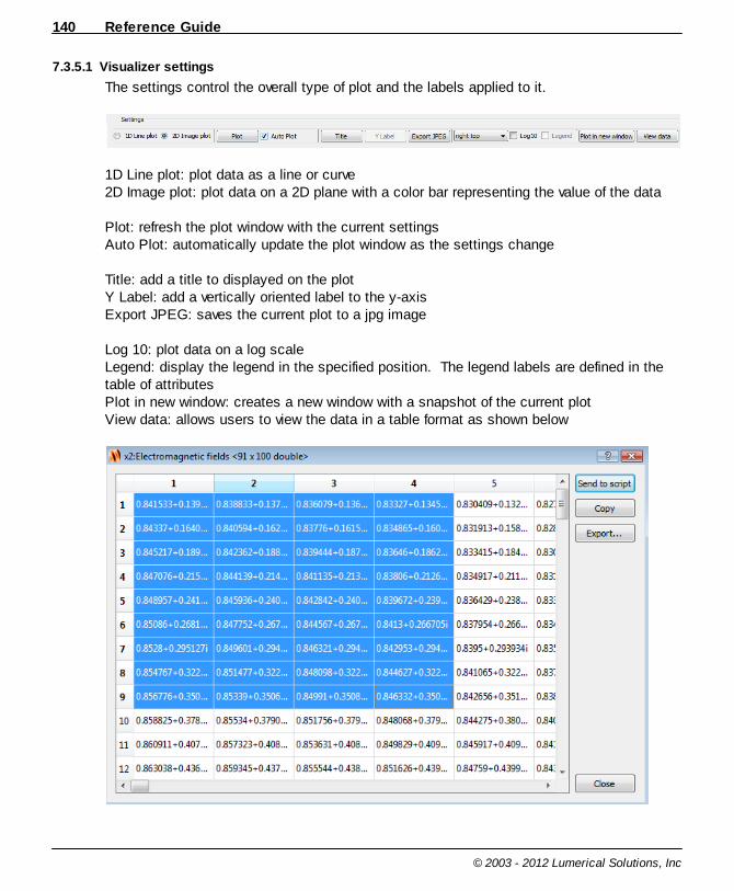
Reference Guide140
© 2003 - 2012 Lumerical Solutions, Inc
7.3.5.1 Visualizer settings
The settings control the overall type of plot and the labels applied to it.
1D Line plot: plot data as a line or curve 2D Image plot: plot data on a 2D plane with a color bar representing the value of the data
Plot: refresh the plot window with the current settingsAuto Plot: automatically update the plot window as the settings change
Title: add a title to displayed on the plotY Label: add a vertically oriented label to the y-axisExport JPEG: saves the current plot to a jpg image
Log 10: plot data on a log scaleLegend: display the legend in the specified position. The legend labels are defined in thetable of attributesPlot in new window: creates a new window with a snapshot of the current plotView data: allows users to view the data in a table format as shown below
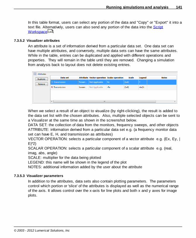
Running simulations and analysis 141
© 2003 - 2012 Lumerical Solutions, Inc
In this table format, users can select any portion of the data and "Copy" or "Export" it into atext file. Alternatively, users can also send any portion of the data into the ScriptWorkspace .
7.3.5.2 Visualizer attributes
An attribute is a set of information derived from a particular data set. One data set canhave multiple attributes, and conversely, multiple data sets can have the same attributes.While in the table, entries can be duplicated and applied with different operations andproperties. They will remain in the table until they are removed. Changing a simulationfrom analysis back to layout does not delete existing entries.
When we select a result of an object to visualize (by right-clicking), the result is added tothe data set list with the chosen attributes. Also, multiple selected objects can be sent toa Visualizer at the same time as shown in the screenshot below.DATA SET: the collection of data from the monitors, frequency sweeps, and other objectsATTRIBUTE: information derived from a particular data set e.g. (a frequency monitor dataset can have E, H, and transmission as attributes)VECTOR OPERATION: selects a particular component of a vector attribute e.g. (Ex, Ey, |E| 2)SCALAR OPERATION: selects a particular component of a scalar attribute e.g. (real,imag, abs, angle)SCALE: multiplier for the data being plottedLEGEND: this name will be shown in the legend of the plotNOTES: additional information added by the user about the attribute
7.3.5.3 Visualizer parameters
In addition to the attributes, data sets also contain plotting parameters. The parameterscontrol which portion or 'slice' of the attributes is displayed as well as the numerical rangeof the axis. It allows control over the x-axis for line plots and both x and y axes for imageplots.
144
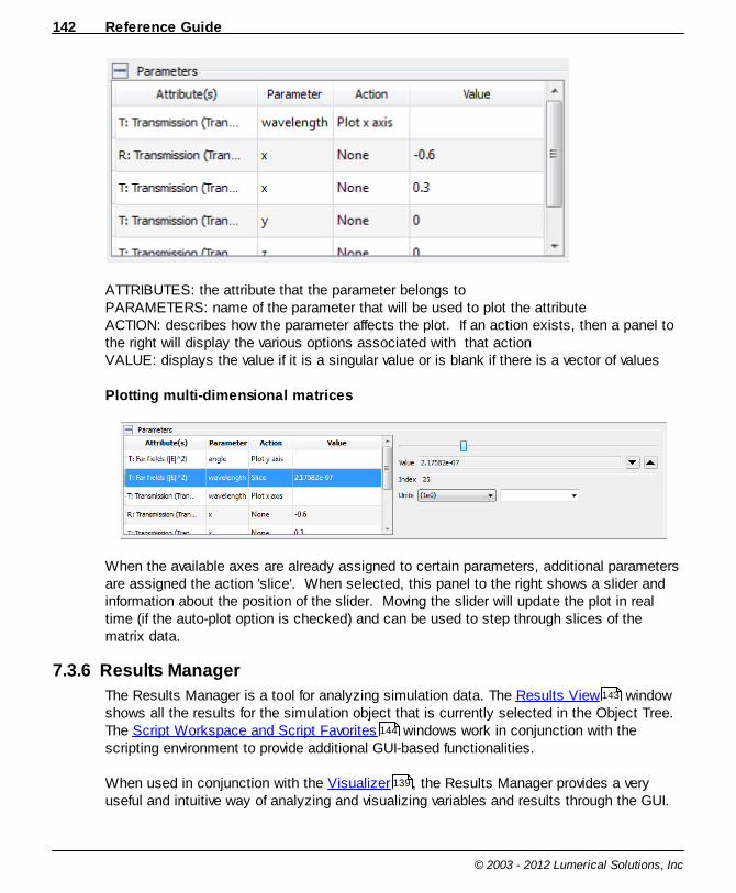
Reference Guide142
© 2003 - 2012 Lumerical Solutions, Inc
ATTRIBUTES: the attribute that the parameter belongs toPARAMETERS: name of the parameter that will be used to plot the attributeACTION: describes how the parameter affects the plot. If an action exists, then a panel tothe right will display the various options associated with that actionVALUE: displays the value if it is a singular value or is blank if there is a vector of values
Plotting multi-dimensional matrices
When the available axes are already assigned to certain parameters, additional parametersare assigned the action 'slice'. When selected, this panel to the right shows a slider andinformation about the position of the slider. Moving the slider will update the plot in realtime (if the auto-plot option is checked) and can be used to step through slices of thematrix data.
7.3.6 Results Manager
The Results Manager is a tool for analyzing simulation data. The Results View windowshows all the results for the simulation object that is currently selected in the Object Tree.The Script Workspace and Script Favorites windows work in conjunction with thescripting environment to provide additional GUI-based functionalities.
When used in conjunction with the Visualizer , the Results Manager provides a veryuseful and intuitive way of analyzing and visualizing variables and results through the GUI.
143
144
139

Running simulations and analysis 143
© 2003 - 2012 Lumerical Solutions, Inc
7.3.6.1 Results View
The Results View window shows all the results for the simulation object that is currentlyselected in the Object Tree. Any simulation object that have results will be displayed witha symbol on the bottom-right corner.
The name of the available results, and the corresponding dimensions or are displayed. Onecan right click on any of the results to display them in the Visualizer , or to send the tothe Script Workspace for further post-processing.
FDTD Solutions 8.0 introduces the use of datasets, allowing one to package raw data intomeaningful results that can be easily parameterized and visualized. The results for all thestandard monitors in FDTD Solutions can be retrieved in the original raw, un-parameterizedmatrix form (using getdata, as in FDTD 7.5), or in dataset form (using getresult). Forexample, in the Results View figure above, the results listed under “rawdata” can beobtained using the “getdata” command. The results listed under "results" are datasets, andcan be obtained using the “getresult” command (these calculations will only be carried outwhen they are visualized). The icons associated with each result reflect the type of result:
Matrix: this is a simple matrix result, with no associated parameters
Matrix dataset: this is a parameterized matrix results that contains at least anattribute (result), and a associated parameter
143
139
144
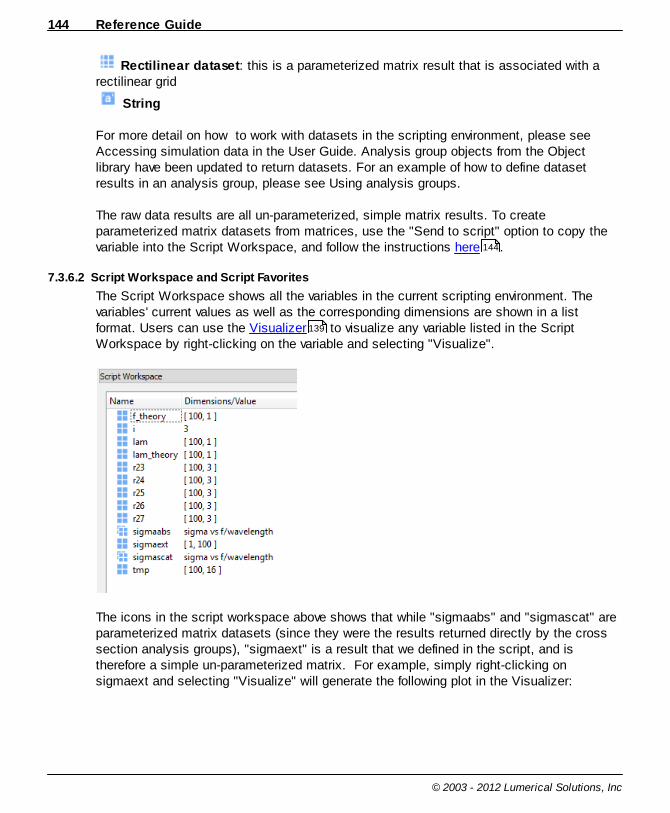
Reference Guide144
© 2003 - 2012 Lumerical Solutions, Inc
Rectilinear dataset: this is a parameterized matrix result that is associated with arectilinear grid
String
For more detail on how to work with datasets in the scripting environment, please see Accessing simulation data in the User Guide. Analysis group objects from the Objectlibrary have been updated to return datasets. For an example of how to define datasetresults in an analysis group, please see Using analysis groups.
The raw data results are all un-parameterized, simple matrix results. To createparameterized matrix datasets from matrices, use the "Send to script" option to copy thevariable into the Script Workspace, and follow the instructions here .
7.3.6.2 Script Workspace and Script Favorites
The Script Workspace shows all the variables in the current scripting environment. Thevariables' current values as well as the corresponding dimensions are shown in a listformat. Users can use the Visualizer to visualize any variable listed in the ScriptWorkspace by right-clicking on the variable and selecting "Visualize".
The icons in the script workspace above shows that while "sigmaabs" and "sigmascat" areparameterized matrix datasets (since they were the results returned directly by the crosssection analysis groups), "sigmaext" is a result that we defined in the script, and istherefore a simple un-parameterized matrix. For example, simply right-clicking onsigmaext and selecting "Visualize" will generate the following plot in the Visualizer:
144
139

Running simulations and analysis 145
© 2003 - 2012 Lumerical Solutions, Inc
Here, the extinction cross section is plotted as a function of the index value. To associate itwith the corresponding frequency array, select the "Create visualization" option, which willopen the "Visualization Creator" dialog window:
This window allows users to set the name of the parameterized variable (sigmaext_vs_f)and its parameters (f). Once this is defined, the visualization creator will generate thecommands necessary for creating the parameterized dataset in the Script Favoriteswindow. When this command is ran, it will send the new parameterized variable to theVisualizer, which will plot the variable as a function of the user specified parameter.
Generated Command Generated Figure
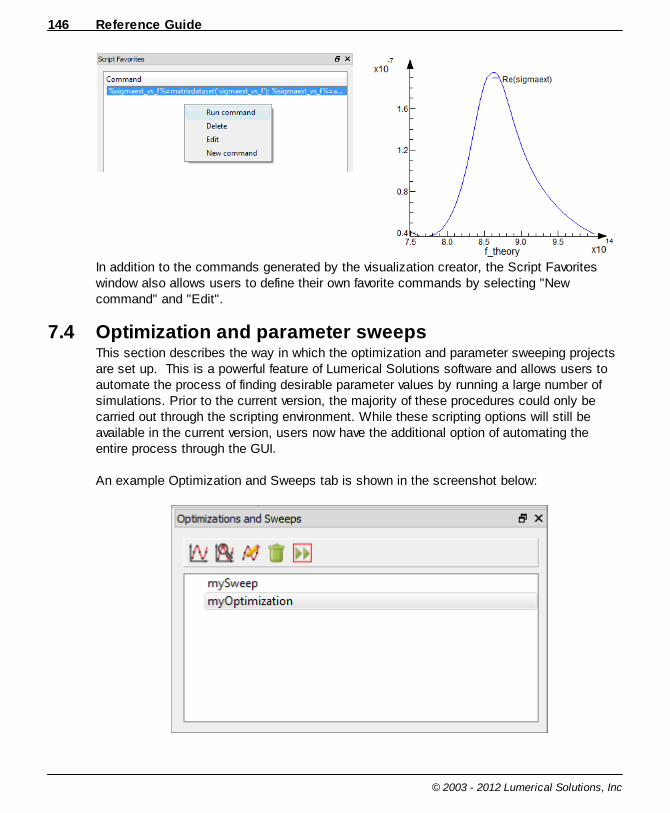
Reference Guide146
© 2003 - 2012 Lumerical Solutions, Inc
In addition to the commands generated by the visualization creator, the Script Favoriteswindow also allows users to define their own favorite commands by selecting "Newcommand" and "Edit".
7.4 Optimization and parameter sweepsThis section describes the way in which the optimization and parameter sweeping projectsare set up. This is a powerful feature of Lumerical Solutions software and allows users toautomate the process of finding desirable parameter values by running a large number ofsimulations. Prior to the current version, the majority of these procedures could only becarried out through the scripting environment. While these scripting options will still beavailable in the current version, users now have the additional option of automating theentire process through the GUI. An example Optimization and Sweeps tab is shown in the screenshot below:

Running simulations and analysis 147
© 2003 - 2012 Lumerical Solutions, Inc
At the top of the window is a toolbar containing the following buttons:
Creates a parameter sweeping project.
Creates an optimization project.
Opens an edit window for the selected project where one can modify its properties.
Deletes the selected project.
Runs the selected sweep or optimization with the resources currently set in theresource manager.
The Animate function allows you to view the structures that will be simulated in a parametersweep or optimization in the CAD before you run the project:

Reference Guide148
© 2003 - 2012 Lumerical Solutions, Inc
7.4.1 Optimization
An example Edit Optimization window is shown in the screen shot below:
The optimization project allows users to use built-in algorithms as well as define their ownoptimization algorithms. For examples on how to set up and run an optimization project,please see Optimize a design. As can be seen from the screenshot above, there is a SETUP tab as well as anADVANCED tab.
Setup Tab
There are three sections in the setup tab:
OPTIMIZATION CONFIGURATION:This section contains the choice of algorithm as well as all the input parameters that areneeded to set up an optimization project using a built-in algorithm:ALGORITHM: The optimization algorithm used for this project
PARTICLE SWARM: The built-in particle swarm algorithm (see Particle SwarmOptimization for more details on the algorithm).
USER DEFINED: The user-defined algorithm specified in the ADVANCED TAB.TYPE: Choice of maximizing or minimizing the figure of meritMAXIMUM GENERATIONS: The maximum number of generations for this optimizationproject.GENERATION SIZE: The generation size (number of child per generation) for this
150
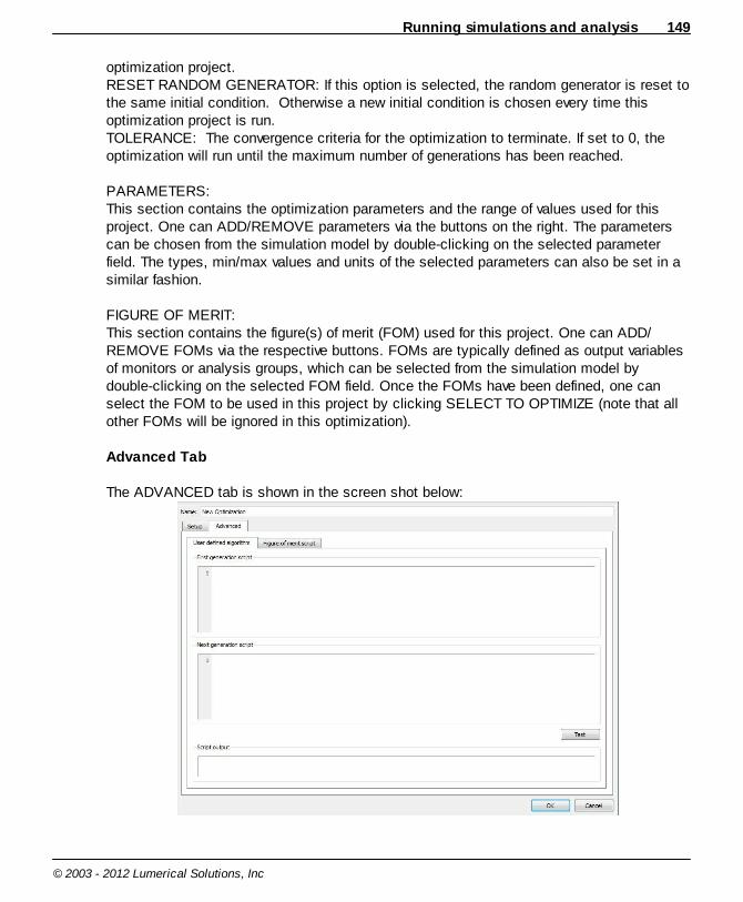
Running simulations and analysis 149
© 2003 - 2012 Lumerical Solutions, Inc
optimization project.RESET RANDOM GENERATOR: If this option is selected, the random generator is reset tothe same initial condition. Otherwise a new initial condition is chosen every time thisoptimization project is run.TOLERANCE: The convergence criteria for the optimization to terminate. If set to 0, theoptimization will run until the maximum number of generations has been reached.
PARAMETERS:This section contains the optimization parameters and the range of values used for thisproject. One can ADD/REMOVE parameters via the buttons on the right. The parameterscan be chosen from the simulation model by double-clicking on the selected parameterfield. The types, min/max values and units of the selected parameters can also be set in asimilar fashion.
FIGURE OF MERIT:This section contains the figure(s) of merit (FOM) used for this project. One can ADD/REMOVE FOMs via the respective buttons. FOMs are typically defined as output variablesof monitors or analysis groups, which can be selected from the simulation model bydouble-clicking on the selected FOM field. Once the FOMs have been defined, one canselect the FOM to be used in this project by clicking SELECT TO OPTIMIZE (note that allother FOMs will be ignored in this optimization).
Advanced Tab
The ADVANCED tab is shown in the screen shot below:
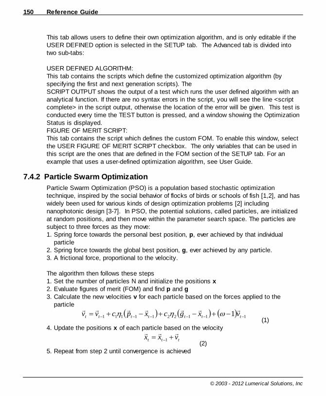
Reference Guide150
© 2003 - 2012 Lumerical Solutions, Inc
This tab allows users to define their own optimization algorithm, and is only editable if theUSER DEFINED option is selected in the SETUP tab. The Advanced tab is divided intotwo sub-tabs:
USER DEFINED ALGORITHM:This tab contains the scripts which define the customized optimization algorithm (byspecifying the first and next generation scripts). The SCRIPT OUTPUT shows the output of a test which runs the user defined algorithm with ananalytical function. If there are no syntax errors in the script, you will see the line <scriptcomplete> in the script output, otherwise the location of the error will be given. This test isconducted every time the TEST button is pressed, and a window showing the OptimizationStatus is displayed. FIGURE OF MERIT SCRIPT:This tab contains the script which defines the custom FOM. To enable this window, selectthe USER FIGURE OF MERIT SCRIPT checkbox. The only variables that can be used inthis script are the ones that are defined in the FOM section of the SETUP tab. For anexample that uses a user-defined optimization algorithm, see User Guide.
7.4.2 Particle Swarm Optimization
Particle Swarm Optimization (PSO) is a population based stochastic optimizationtechnique, inspired by the social behavior of flocks of birds or schools of fish [1,2], and haswidely been used for various kinds of design optimization problems [2] includingnanophotonic design [3-7]. In PSO, the potential solutions, called particles, are initializedat random positions, and then move within the parameter search space. The particles aresubject to three forces as they move:1. Spring force towards the personal best position, p, ever achieved by that individual
particle2. Spring force towards the global best position, g, ever achieved by any particle.3. A frictional force, proportional to the velocity.
The algorithm then follows these steps1. Set the number of particles N and initialize the positions x 2. Evaluate figures of merit (FOM) and find p and g 3. Calculate the new velocities v for each particle based on the forces applied to the
particle
1112211111 1 ttttttt vxgcxpcvv (1)
4. Update the positions x of each particle based on the velocity
ttt vxx 1 (2)
5. Repeat from step 2 until convergence is achieved

Running simulations and analysis 151
© 2003 - 2012 Lumerical Solutions, Inc
In Eq. (1), t is the iteration counter; c1 and c
2 are the cognitive and social factors,
respectively; ω is called the inertial weight; and η1 and η
2 are random number between 0
and 1. Lumerical's PSO implementation uses default values of c1, c
2 and ω that have
shown to converge well in many test optimization problems for photonic design problems. Adetailed description of the algorithm and the difference coefficients can be found in Refs. [1]or [2].J. Robinson and Y. Rahmat-Samii, "Particle swarm optimization in Electromagnetics,"IEEE Trans. Antennas and Propagat. 52, pp.397 - 407 (2004).1. K. E. Parsopoulo and M N. Vrahatis, Particle swarm optimization and intelligence :
advances and applications, Information Science Reference, 2010.2. J. Pond and M. Kawano, “Virtual prototyping and optimization of novel solar cell
designs”, Proc. SPIE 7750, 775028 (2010), DOI:10.1117/12.8731143. M. Kawano and J. Pond, "Design Optimization of Photonic Crystal Organic Solar Cells
using the FDTD method in Combination with Particle Swarm Optimization," 7thInternational Conference on Optics-photonics Design & Fabrication, Yokohama, Japan,19S1-14, 2010.
4. J. G. Mutitu, S. Shi, C. Chen, T. Creazzo, A. Barnett, C. Honsberg and D. W. Prather,"Thin film silicon solar cell design based on photonic crystal and diffractive gratingstructures", Opt. Express 16, 5238, 2008
5. M.Shokooh-Saremi and R. Magnusson, "Leaky-mode resonant reflectors with extremebandwidths," Opt. Lett. 35, 1121, 2010.
6. R. Magnusson, M. Shokooh-Saremi,and E. G. Johnson, “Guided-mode resonant waveplates,” Opt. Lett. 35, 2472, 2010.

Reference Guide152
© 2003 - 2012 Lumerical Solutions, Inc
7.4.3 Parameter Sweeps
An example Edit Parameter Sweep window is shown in the screen shot below:
For examples on how to set up and run a parameter sweep project, please see Run aparameter sweep.
There are two sections in the Edit Parameter Sweep window:
PARAMETERS:This section contains all the input parameters that are needed to set up a parameter sweepproject. There are two ways to specify the inputs to the parameter sweep. If RANGES isselected, the table above is shown. One can ADD/REMOVE parameters via the respectivebutton on the right. The parameters can be chosen from the simulation model by double-clicking on the selected parameter field, and the types, min/max values and units of theselected parameters can be set in a similar fashion. If VALUES is selected, the followingtable is shown:
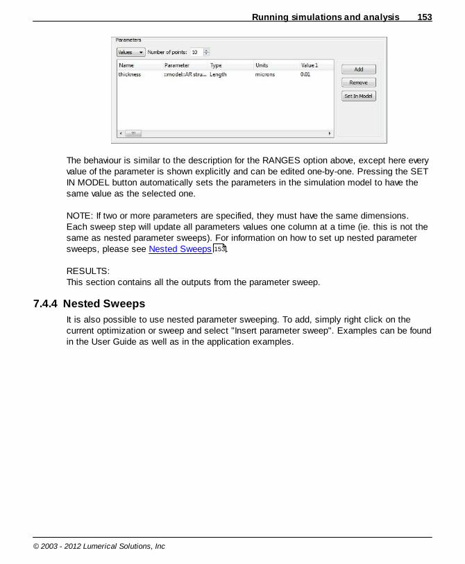
Running simulations and analysis 153
© 2003 - 2012 Lumerical Solutions, Inc
The behaviour is similar to the description for the RANGES option above, except here everyvalue of the parameter is shown explicitly and can be edited one-by-one. Pressing the SETIN MODEL button automatically sets the parameters in the simulation model to have thesame value as the selected one.
NOTE: If two or more parameters are specified, they must have the same dimensions. Each sweep step will update all parameters values one column at a time (ie. this is not thesame as nested parameter sweeps). For information on how to set up nested parametersweeps, please see Nested Sweeps .
RESULTS:This section contains all the outputs from the parameter sweep.
7.4.4 Nested Sweeps
It is also possible to use nested parameter sweeping. To add, simply right click on thecurrent optimization or sweep and select "Insert parameter sweep". Examples can be foundin the User Guide as well as in the application examples.
153
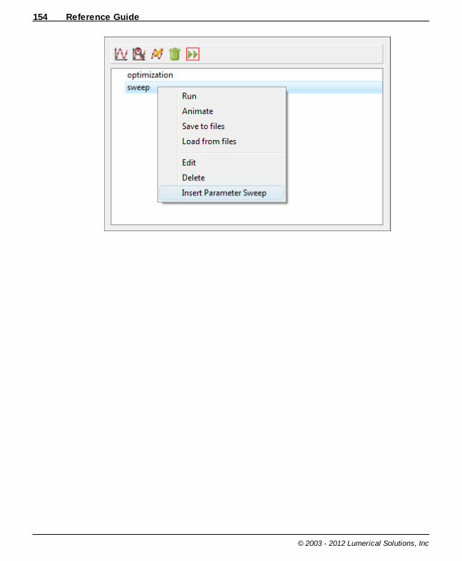
Reference Guide154
© 2003 - 2012 Lumerical Solutions, Inc
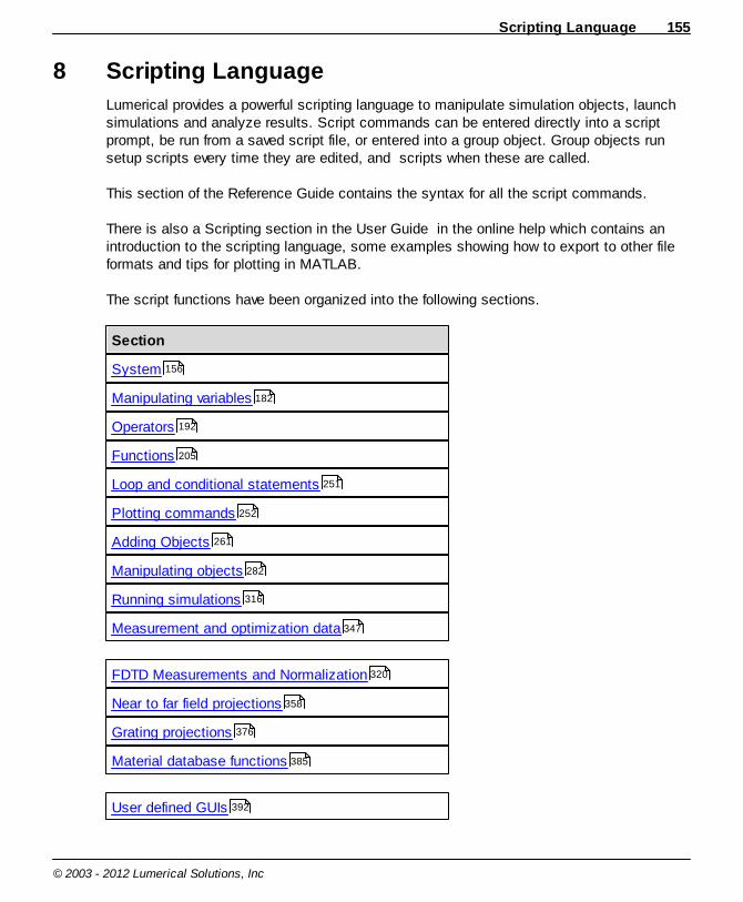
Scripting Language 155
© 2003 - 2012 Lumerical Solutions, Inc
8 Scripting Language
Lumerical provides a powerful scripting language to manipulate simulation objects, launchsimulations and analyze results. Script commands can be entered directly into a scriptprompt, be run from a saved script file, or entered into a group object. Group objects runsetup scripts every time they are edited, and scripts when these are called.
This section of the Reference Guide contains the syntax for all the script commands.
There is also a Scripting section in the User Guide in the online help which contains anintroduction to the scripting language, some examples showing how to export to other fileformats and tips for plotting in MATLAB.
The script functions have been organized into the following sections.
Section
System
Manipulating variables
Operators
Functions
Loop and conditional statements
Plotting commands
Adding Objects
Manipulating objects
Running simulations
Measurement and optimization data
FDTD Measurements and Normalization
Near to far field projections
Grating projections
Material database functions
User defined GUIs
156
182
192
205
251
252
261
282
316
347
320
358
376
385
392

Reference Guide156
© 2003 - 2012 Lumerical Solutions, Inc
Creating your own script commands
The online help version of the Scripting Language section includes examples for many ofthe script functions.
8.1 SystemSystem commands for interacting with the OS file system, running script files, etc.
System commands
Command Description
new2d Creates a new 2D FDTD layout environment.
new3d Creates a new 3D FDTD layout environment.
newmode Creates a new MODE layout environment.
save Saves an fsp file or lms file.
load Loads an fsp file or lms file.
delrm
Deletes a file.
ls dir
Lists the files in a directory.
cd Changes the working directory.
pwd Returns the current working directory.
cp Copy a file.
mv Move a file
exit Exit the application.
system Run command prompts.
fileexists Check if a file exists.
currentfilename Get the current filename.
filebasename Get the file base name from a string.
filedirectory Get the file directory from a string.
fileextension Get the file extension from a string.
List of script commands
398
159
159
160
161
161
162
162
163
162
163
164
164
165
165
166
166
167
167
168
168
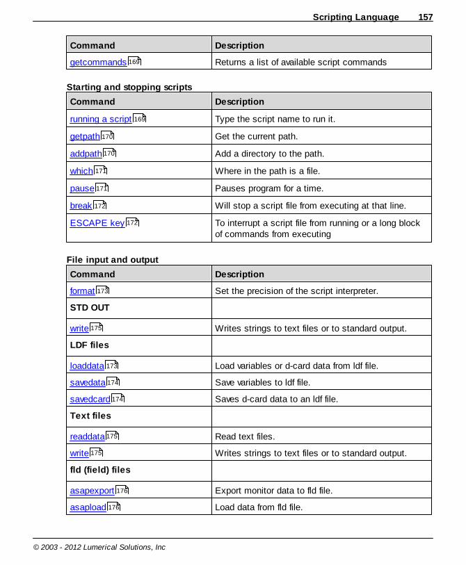
Scripting Language 157
© 2003 - 2012 Lumerical Solutions, Inc
Command Description
getcommands Returns a list of available script commands
Starting and stopping scripts
Command Description
running a script Type the script name to run it.
getpath Get the current path.
addpath Add a directory to the path.
which Where in the path is a file.
pause Pauses program for a time.
break Will stop a script file from executing at that line.
ESCAPE key To interrupt a script file from running or a long blockof commands from executing
File input and output
Command Description
format Set the precision of the script interpreter.
STD OUT
write Writes strings to text files or to standard output.
LDF files
loaddata Load variables or d-card data from ldf file.
savedata Save variables to ldf file.
savedcard Saves d-card data to an ldf file.
Text files
readdata Read text files.
write Writes strings to text files or to standard output.
fld (field) files
asapexport Export monitor data to fld file.
asapload Load data from fld file.
169
169
170
170
171
171
172
172
173
175
173
174
174
175
175
176
176
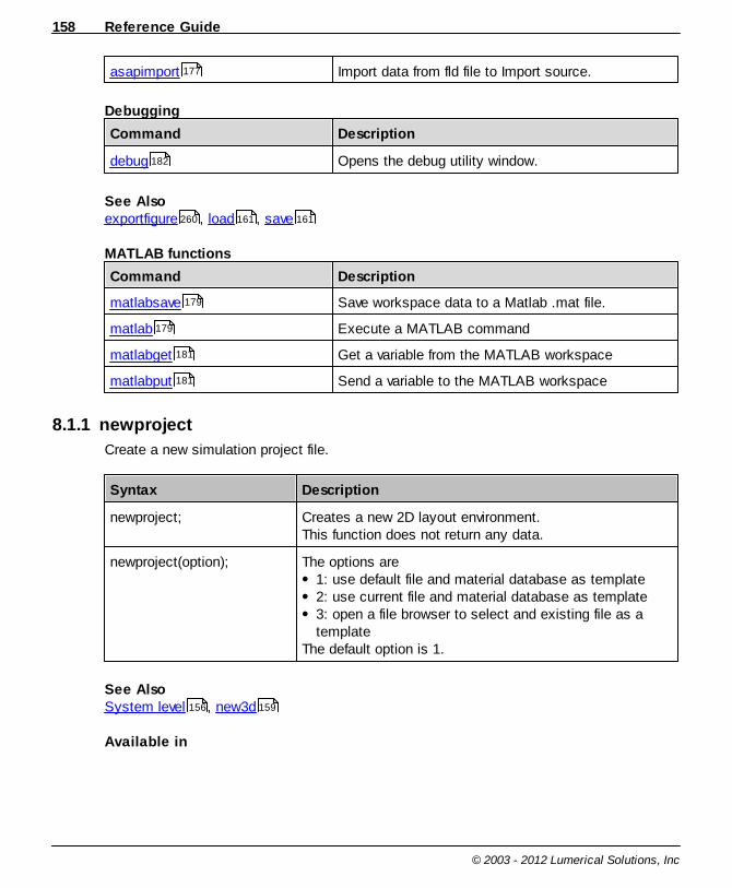
Reference Guide158
© 2003 - 2012 Lumerical Solutions, Inc
asapimport Import data from fld file to Import source.
Debugging
Command Description
debug Opens the debug utility window.
See Also exportfigure , load , save
MATLAB functions
Command Description
matlabsave Save workspace data to a Matlab .mat file.
matlab Execute a MATLAB command
matlabget Get a variable from the MATLAB workspace
matlabput Send a variable to the MATLAB workspace
8.1.1 newproject
Create a new simulation project file.
Syntax Description
newproject; Creates a new 2D layout environment.This function does not return any data.
newproject(option); The options are 1: use default file and material database as template 2: use current file and material database as template 3: open a file browser to select and existing file as atemplate
The default option is 1.
See Also System level , new3d
Available in
177
182
260 161 161
179
179
181
181
156 159
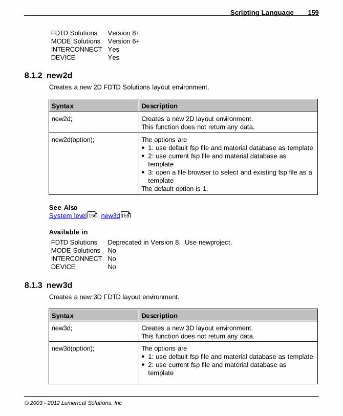
Scripting Language 159
© 2003 - 2012 Lumerical Solutions, Inc
FDTD SolutionsMODE SolutionsINTERCONNECTDEVICE
Version 8+Version 6+YesYes
8.1.2 new2d
Creates a new 2D FDTD Solutions layout environment.
Syntax Description
new2d; Creates a new 2D layout environment.This function does not return any data.
new2d(option); The options are 1: use default fsp file and material database as template 2: use current fsp file and material database astemplate 3: open a file browser to select and existing fsp file as atemplate
The default option is 1.
See Also System level , new3d
Available in
FDTD SolutionsMODE SolutionsINTERCONNECTDEVICE
Deprecated in Version 8. Use newproject.NoNoNo
8.1.3 new3d
Creates a new 3D FDTD layout environment.
Syntax Description
new3d; Creates a new 3D layout environment.This function does not return any data.
new3d(option); The options are 1: use default fsp file and material database as template 2: use current fsp file and material database astemplate
156 159
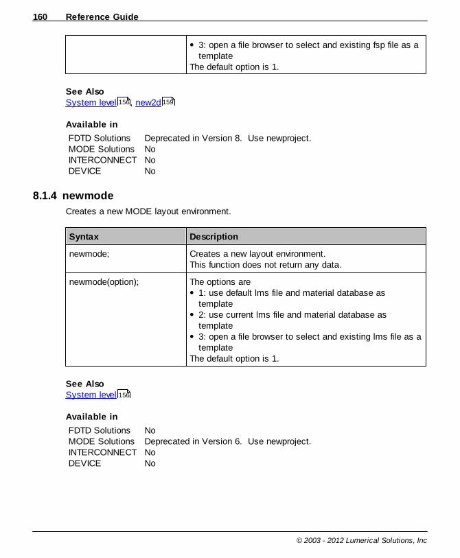
Reference Guide160
© 2003 - 2012 Lumerical Solutions, Inc
3: open a file browser to select and existing fsp file as atemplate
The default option is 1.
See Also System level , new2d
Available in
FDTD SolutionsMODE SolutionsINTERCONNECTDEVICE
Deprecated in Version 8. Use newproject.NoNoNo
8.1.4 newmode
Creates a new MODE layout environment.
Syntax Description
newmode; Creates a new layout environment.This function does not return any data.
newmode(option); The options are 1: use default lms file and material database astemplate 2: use current lms file and material database astemplate 3: open a file browser to select and existing lms file as atemplate
The default option is 1.
See AlsoSystem level
Available in
FDTD SolutionsMODE SolutionsINTERCONNECTDEVICE
NoDeprecated in Version 6. Use newproject.NoNo
156 159
156
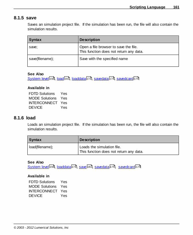
Scripting Language 161
© 2003 - 2012 Lumerical Solutions, Inc
8.1.5 save
Saves an simulation project file. If the simulation has been run, the file will also contain thesimulation results.
Syntax Description
save; Open a file browser to save the file.This function does not return any data.
save(filename); Save with the specified name
See Also System level , load , loaddata , savedata , savedcard
Available in
FDTD SolutionsMODE SolutionsINTERCONNECTDEVICE
YesYesYesYes
8.1.6 load
Loads an simulation project file. If the simulation has been run, the file will also contain thesimulation results.
Syntax Description
load(filename); Loads the simulation file.This function does not return any data.
See Also System level , loaddata , save , savedata , savedcard
Available in
FDTD SolutionsMODE SolutionsINTERCONNECTDEVICE
YesYesYesYes
156 161 173 174 174
156 173 161 174 174

Reference Guide162
© 2003 - 2012 Lumerical Solutions, Inc
8.1.7 del
Delete a file.
Syntax Description
del("filename"); rm("filename");
Deletes the file "filename".This function does not return any data.
See AlsoSystem level , delete
Available in
FDTD SolutionsMODE SolutionsINTERCONNECTDEVICE
YesYesYesYes
8.1.8 rm
Delete a file.
Syntax Description
del("filename"); rm("filename");
Deletes the file "filename".This function does not return any data.
See AlsoSystem level , delete
Available in
FDTD SolutionsMODE SolutionsINTERCONNECTDEVICE
YesYesYesYes
8.1.9 dir
List files in a directory.
Syntax Description
out = dir; The output is a string.
156 285
156 285

Scripting Language 163
© 2003 - 2012 Lumerical Solutions, Inc
out = ls; Use ?dir; to write the value to the screen.
out = dir("directory"); out = ls("directory");
Lists the files in the specified directory.
See AlsoSystem level
Available in
FDTD SolutionsMODE SolutionsINTERCONNECTDEVICE
YesYesYesYes
8.1.10 ls
List files in a directory.
Syntax Description
out = dir; out = ls;
The output is a string.Use ?dir; to write the value to the screen.
out = dir("directory"); out = ls("directory");
Lists the files in the specified directory.
See AlsoSystem level
Available in
FDTD SolutionsMODE SolutionsINTERCONNECTDEVICE
YesYesYesYes
8.1.11 cd
Change directory.
Syntax Description
cd; Opens a window to browse to a directory.This function does not return any data.
156
156
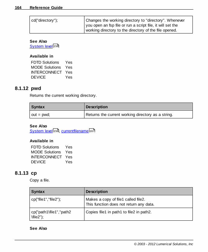
Reference Guide164
© 2003 - 2012 Lumerical Solutions, Inc
cd("directory"); Changes the working directory to "directory". Wheneveryou open an fsp file or run a script file, it will set theworking directory to the directory of the file opened.
See AlsoSystem level
Available in
FDTD SolutionsMODE SolutionsINTERCONNECTDEVICE
YesYesYesYes
8.1.12 pwd
Returns the current working directory.
Syntax Description
out = pwd; Returns the current working directory as a string.
See AlsoSystem level , currentfilename
Available in
FDTD SolutionsMODE SolutionsINTERCONNECTDEVICE
YesYesYesYes
8.1.13 cp
Copy a file.
Syntax Description
cp("file1","file2"); Makes a copy of file1 called file2. This function does not return any data.
cp("path1\file1","path2\file2");
Copies file1 in path1 to file2 in path2.
See Also
156
156 167

Scripting Language 165
© 2003 - 2012 Lumerical Solutions, Inc
System level , mv , pwd , copy (objects)
Available in
FDTD SolutionsMODE SolutionsINTERCONNECTDEVICE
YesYesYesYes
8.1.14 mv
Move a file.
Syntax Description
mv("file1","file2"); Moves file1 to file2. This function does not return any data.
cp("path1\file1","path2\file2");
Moves file1 in path1 to file2 in path2.
See AlsoSystem level , cp , pwd
Available in
FDTD SolutionsMODE SolutionsINTERCONNECTDEVICE
YesYesYesYes
8.1.15 exit
Exit the application.
Syntax Description
exit; Exits the application. Same as exit(1);This function does not return any data.
exit(option); Exits the application. The option can be 1: Prompt user if a file needs saving before exiting. 2: Force the application to exit without prompting theuser.
The default option is 1.
156 165 164 290
156 164 164
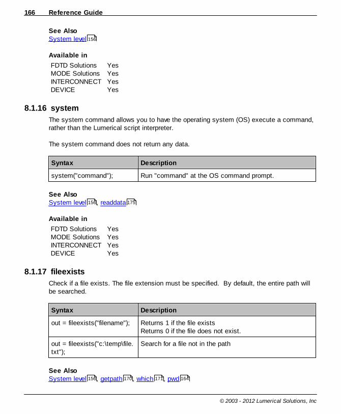
Reference Guide166
© 2003 - 2012 Lumerical Solutions, Inc
See AlsoSystem level
Available in
FDTD SolutionsMODE SolutionsINTERCONNECTDEVICE
YesYesYesYes
8.1.16 system
The system command allows you to have the operating system (OS) execute a command,rather than the Lumerical script interpreter.
The system command does not return any data.
Syntax Description
system("command"); Run "command" at the OS command prompt.
See AlsoSystem level , readdata
Available in
FDTD SolutionsMODE SolutionsINTERCONNECTDEVICE
YesYesYesYes
8.1.17 fileexists
Check if a file exists. The file extension must be specified. By default, the entire path willbe searched.
Syntax Description
out = fileexists("filename"); Returns 1 if the file existsReturns 0 if the file does not exist.
out = fileexists("c:\temp\file.txt");
Search for a file not in the path
See AlsoSystem level , getpath , which , pwd
156
156 175
156 170 171 164

Scripting Language 167
© 2003 - 2012 Lumerical Solutions, Inc
Available in
FDTD SolutionsMODE SolutionsINTERCONNECTDEVICE
YesYesYesYes
8.1.18 currentfilename
Get the current filename and directory.
Syntax Description
out = currentfilename; Returns the current filename as a string. If the current filename is not defined, this function returnsan empty string "".
See AlsoSystem level , fileexists , getpath , which , pwd , fileextension ,filebasename , filedirectory
Available in
FDTD SolutionsMODE SolutionsINTERCONNECTDEVICE
YesYesYesYes
8.1.19 filebasename
Get the file basename from a string.
Syntax Description
out = filebasename( "location/filename.ext" );
Returns the file basename as a string.
See AlsoSystem level , currentfilename , getpath , which , pwd
Available in
156 166 170 171 164 168
167 168
156 167 170 171 164

Reference Guide168
© 2003 - 2012 Lumerical Solutions, Inc
FDTD SolutionsMODE SolutionsINTERCONNECTDEVICE
YesYesYesYes
8.1.20 fileextension
Get the file extension from a string.
Syntax Description
out = fileextension( "name.ext");
Returns the file extension as a string.
See AlsoSystem level , currentfilename , getpath , which , pwd
Available in
FDTD SolutionsMODE SolutionsINTERCONNECTDEVICE
YesYesYesYes
8.1.21 filedirectory
Get the file directory from a string.
Syntax Description
out = filedirectory( "location/filename.ext" );
Returns the file directory as a string.
See AlsoSystem level , currentfilename , getpath , which , pwd
Available in
FDTD SolutionsMODE SolutionsINTERCONNECTDEVICE
YesYesYesYes
156 167 170 171 164
156 167 170 171 164

Scripting Language 169
© 2003 - 2012 Lumerical Solutions, Inc
8.1.22 getcommands
Returns the list of available script commands in the current script workspace.
Syntax Description
?getcommands; Returns a list of available script commands
See AlsoSystem level
Available in
FDTD SolutionsMODE SolutionsINTERCONNECTDEVICE
YesYesYesYes
8.1.23 Run script
Run a script by typing its name. The file must be in the current path. The path alwayssearches the current directory first. A script file is not passed variables, and does notreturn variables. All scripts have access to all of the variables defined in the currentworkspace.
It's best to avoid using the names of Lumerical script functions (i.e. plot) for the names ofyour script files. If a script file has the same name as a function, the script will be run (notthe function). This allows you to effectively re-define the behavior of a function, but it cancause confusion when done unintentionally.
Syntax Description
filename; Run the script file filename.lsf, if it exists in the currentpath.A script does not have a return type.
See AlsoSystem level , getpath , addpath , which
Available in
156
156 170 170 171

Reference Guide170
© 2003 - 2012 Lumerical Solutions, Inc
FDTD SolutionsMODE SolutionsINTERCONNECTDEVICE
YesYesYesYes
8.1.24 getpath
Get the current path. By default, the current working directory and the script sub-directoryof the installation (eg. C:\Program Files\Lumerical\FDTD\scripts) are in the path.
Syntax Description
out = getpath; Returns the current path as a string. Use ?getpath; to print it to the screen.
See AlsoSystem level , addpath , which , pwd
Available in
FDTD SolutionsMODE SolutionsINTERCONNECTDEVICE
YesYesYesYes
8.1.25 addpath
Add a directory to the path.
Syntax Description
addpath("directory"); Adds a directory to the path. This function does not return any data.
See AlsoSystem level , getpath , which , pwd
Available in
FDTD SolutionsMODE SolutionsINTERCONNECTDEVICE
YesYesYesYes
156 170 171 164
156 170 171 164
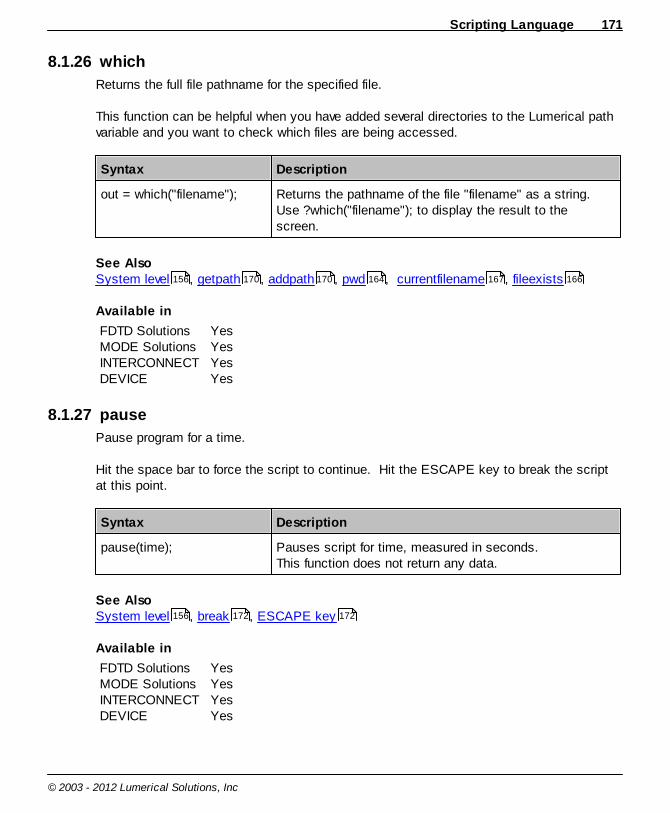
Scripting Language 171
© 2003 - 2012 Lumerical Solutions, Inc
8.1.26 which
Returns the full file pathname for the specified file.
This function can be helpful when you have added several directories to the Lumerical pathvariable and you want to check which files are being accessed.
Syntax Description
out = which("filename"); Returns the pathname of the file "filename" as a string. Use ?which("filename"); to display the result to thescreen.
See AlsoSystem level , getpath , addpath , pwd , currentfilename , fileexists
Available in
FDTD SolutionsMODE SolutionsINTERCONNECTDEVICE
YesYesYesYes
8.1.27 pause
Pause program for a time.
Hit the space bar to force the script to continue. Hit the ESCAPE key to break the scriptat this point.
Syntax Description
pause(time); Pauses script for time, measured in seconds.This function does not return any data.
See AlsoSystem level , break , ESCAPE key
Available in
FDTD SolutionsMODE SolutionsINTERCONNECTDEVICE
YesYesYesYes
156 170 170 164 167 166
156 172 172
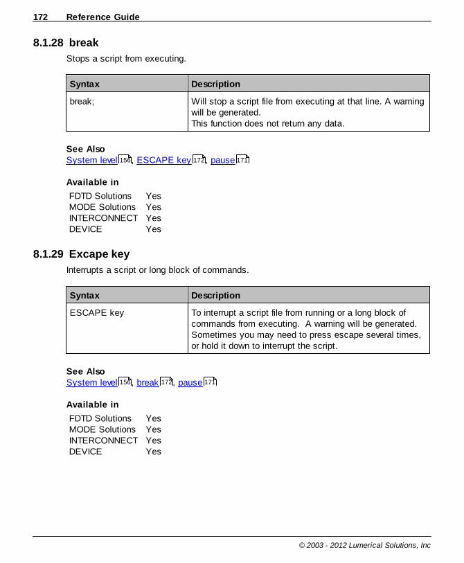
Reference Guide172
© 2003 - 2012 Lumerical Solutions, Inc
8.1.28 break
Stops a script from executing.
Syntax Description
break; Will stop a script file from executing at that line. A warningwill be generated.This function does not return any data.
See AlsoSystem level , ESCAPE key , pause
Available in
FDTD SolutionsMODE SolutionsINTERCONNECTDEVICE
YesYesYesYes
8.1.29 Excape key
Interrupts a script or long block of commands.
Syntax Description
ESCAPE key To interrupt a script file from running or a long block ofcommands from executing. A warning will be generated. Sometimes you may need to press escape several times,or hold it down to interrupt the script.
See AlsoSystem level , break , pause
Available in
FDTD SolutionsMODE SolutionsINTERCONNECTDEVICE
YesYesYesYes
156 172 171
156 172 171

Scripting Language 173
© 2003 - 2012 Lumerical Solutions, Inc
8.1.30 format
The two format commands toggle the script interpreter between 2 output precision states.The commands print (?) and num2str() use this state to determine how many digits ofprecision to output.
Syntax Description
format long; Set script interpreter to 16 digits of precision.
format short; Set script interpreter to 6 digits of precision.
See AlsoSystem level , num2str , ?
Available in
FDTD SolutionsMODE SolutionsINTERCONNECTDEVICE
YesYesYesYes
8.1.31 loaddata
Loads workspace variables or d-card data from a Lumerical data file (ldf) file. If any currentvariables exist with the same names as those in the file, the current values will beoverwritten.
Syntax Description
loaddata("filename"); Reads data script variables or d-card data from thespecified file. This function does not return any data.
See AlsoSystem level , savedata , savedcard , workspace , load
Available in
FDTD SolutionsMODE SolutionsINTERCONNECTDEVICE
YesYesYesYes
156 229 204
156 174 174 189 161
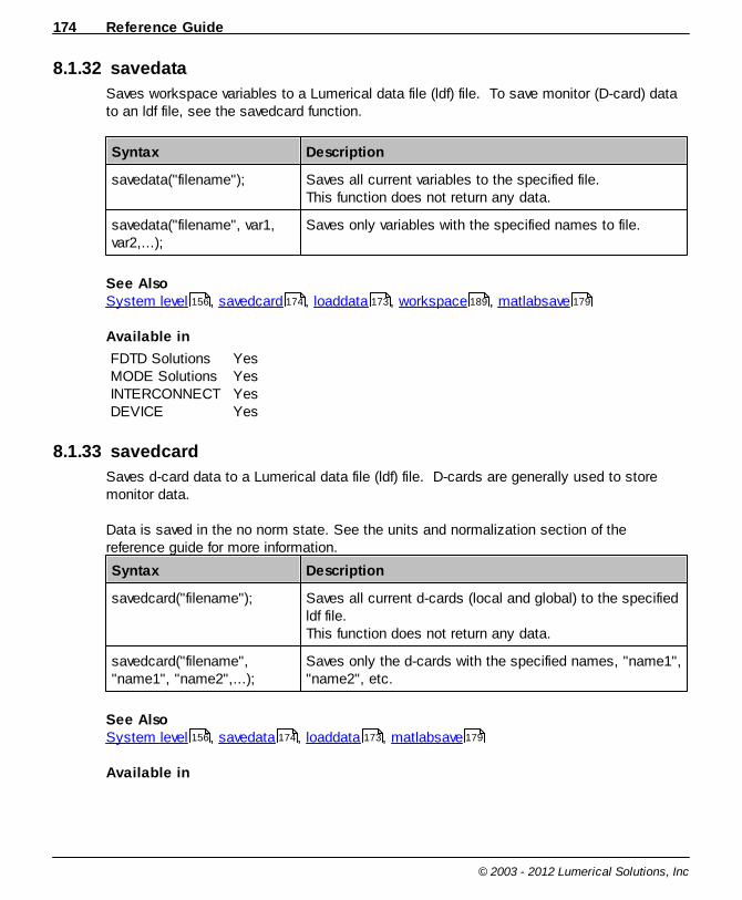
Reference Guide174
© 2003 - 2012 Lumerical Solutions, Inc
8.1.32 savedata
Saves workspace variables to a Lumerical data file (ldf) file. To save monitor (D-card) datato an ldf file, see the savedcard function.
Syntax Description
savedata("filename"); Saves all current variables to the specified file. This function does not return any data.
savedata("filename", var1,var2,...);
Saves only variables with the specified names to file.
See AlsoSystem level , savedcard , loaddata , workspace , matlabsave
Available in
FDTD SolutionsMODE SolutionsINTERCONNECTDEVICE
YesYesYesYes
8.1.33 savedcard
Saves d-card data to a Lumerical data file (ldf) file. D-cards are generally used to storemonitor data.
Data is saved in the no norm state. See the units and normalization section of thereference guide for more information.
Syntax Description
savedcard("filename"); Saves all current d-cards (local and global) to the specifiedldf file.This function does not return any data.
savedcard("filename","name1", "name2",...);
Saves only the d-cards with the specified names, "name1","name2", etc.
See AlsoSystem level , savedata , loaddata , matlabsave
Available in
156 174 173 189 179
156 174 173 179
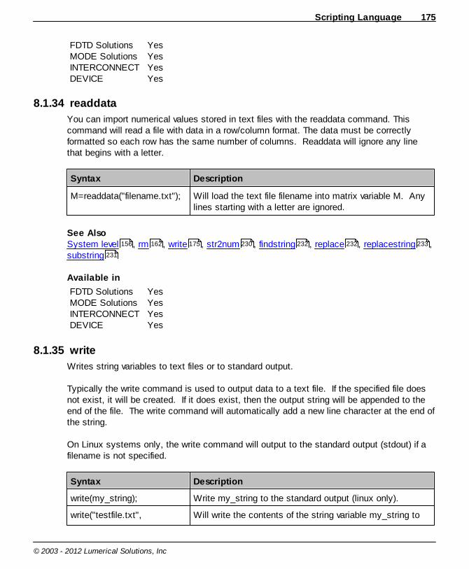
Scripting Language 175
© 2003 - 2012 Lumerical Solutions, Inc
FDTD SolutionsMODE SolutionsINTERCONNECTDEVICE
YesYesYesYes
8.1.34 readdata
You can import numerical values stored in text files with the readdata command. Thiscommand will read a file with data in a row/column format. The data must be correctlyformatted so each row has the same number of columns. Readdata will ignore any linethat begins with a letter.
Syntax Description
M=readdata("filename.txt"); Will load the text file filename into matrix variable M. Anylines starting with a letter are ignored.
See AlsoSystem level , rm , write , str2num , findstring , replace , replacestring ,substring
Available in
FDTD SolutionsMODE SolutionsINTERCONNECTDEVICE
YesYesYesYes
8.1.35 write
Writes string variables to text files or to standard output.
Typically the write command is used to output data to a text file. If the specified file doesnot exist, it will be created. If it does exist, then the output string will be appended to theend of the file. The write command will automatically add a new line character at the end ofthe string.
On Linux systems only, the write command will output to the standard output (stdout) if afilename is not specified.
Syntax Description
write(my_string); Write my_string to the standard output (linux only).
write("testfile.txt", Will write the contents of the string variable my_string to
156 162 175 230 232 232 233
231

Reference Guide176
© 2003 - 2012 Lumerical Solutions, Inc
my_string); testfile.txt.This function does not return any data.
See AlsoSystem level , readdata , rm , num2str , ? , endl , format
Available in
FDTD SolutionsMODE SolutionsINTERCONNECTDEVICE
YesYesYesYes
8.1.36 asapexport
Exports the desired monitor to a file for interfacing with BRO's ASAP. These files are calledfld files. The monitor must be a frequency power or a frequency profile monitor.
Syntax Description
asapexport( "monitorname"); Export data from monitorname. By default, the firstfrequency point is exported. This function does not return any data.
asapexport( "monitorname",f);
Exports the frequency point specified by the index f.
asapexport( "monitorname",f, "filename");
Exports to the specified "filename" without opening a filebrowser window.
See AlsoSystem level , asapload , asapimport , addimportedsource
Available in
FDTD SolutionsMODE SolutionsINTERCONNECTDEVICE
YesYesNoNo
8.1.37 asapload
Load data from an fld file from BRO's ASAP. asapload creates a d-card structure called"fld_data" which contains all the data in the file. If "fld_data" exists, it will be called"fld_data_2". After loading an asapfile with asapload, you can extract any desired data.,which can be
156 175 162 229 204 204 173
156 176 177 275
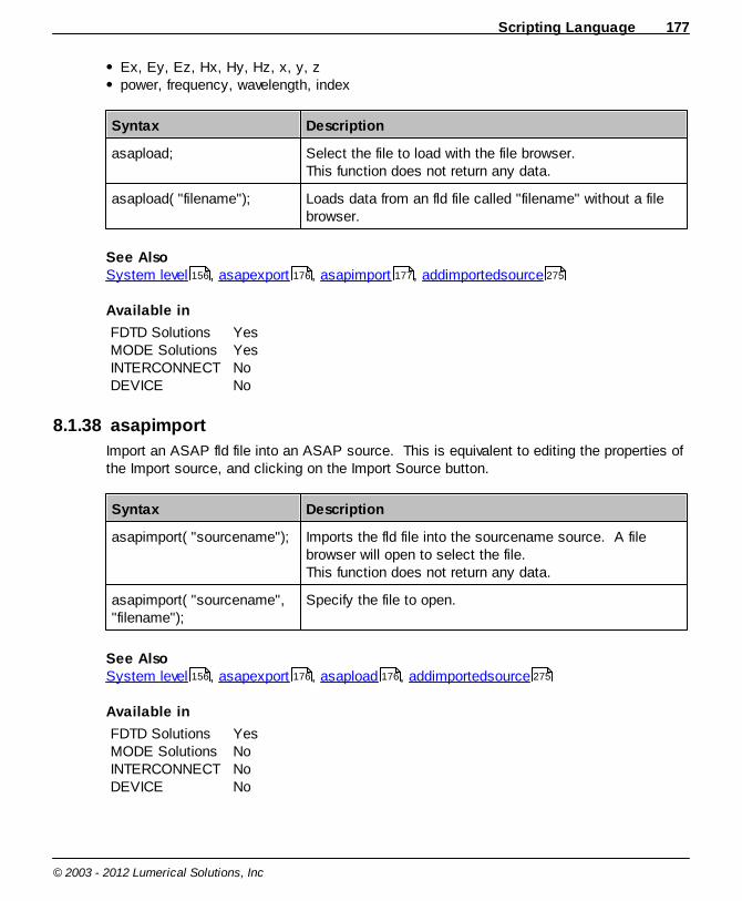
Scripting Language 177
© 2003 - 2012 Lumerical Solutions, Inc
Ex, Ey, Ez, Hx, Hy, Hz, x, y, z power, frequency, wavelength, index
Syntax Description
asapload; Select the file to load with the file browser.This function does not return any data.
asapload( "filename"); Loads data from an fld file called "filename" without a filebrowser.
See AlsoSystem level , asapexport , asapimport , addimportedsource
Available in
FDTD SolutionsMODE SolutionsINTERCONNECTDEVICE
YesYesNoNo
8.1.38 asapimport
Import an ASAP fld file into an ASAP source. This is equivalent to editing the properties ofthe Import source, and clicking on the Import Source button.
Syntax Description
asapimport( "sourcename"); Imports the fld file into the sourcename source. A filebrowser will open to select the file.This function does not return any data.
asapimport( "sourcename","filename");
Specify the file to open.
See AlsoSystem level , asapexport , asapload , addimportedsource
Available in
FDTD SolutionsMODE SolutionsINTERCONNECTDEVICE
YesNoNoNo
156 176 177 275
156 176 176 275
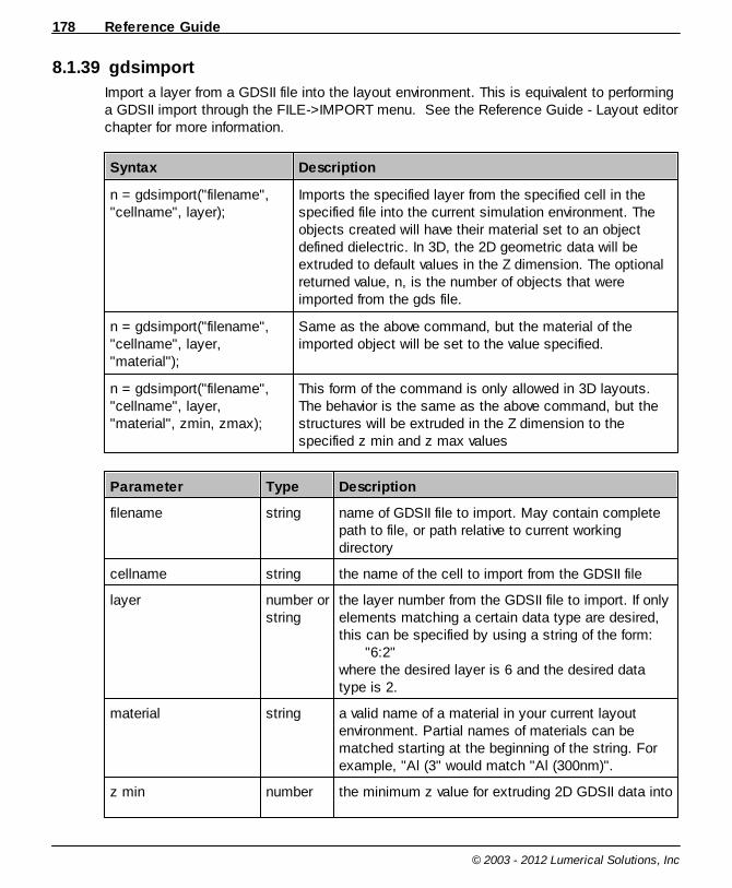
Reference Guide178
© 2003 - 2012 Lumerical Solutions, Inc
8.1.39 gdsimport
Import a layer from a GDSII file into the layout environment. This is equivalent to performinga GDSII import through the FILE->IMPORT menu. See the Reference Guide - Layout editorchapter for more information.
Syntax Description
n = gdsimport("filename","cellname", layer);
Imports the specified layer from the specified cell in thespecified file into the current simulation environment. Theobjects created will have their material set to an objectdefined dielectric. In 3D, the 2D geometric data will beextruded to default values in the Z dimension. The optionalreturned value, n, is the number of objects that wereimported from the gds file.
n = gdsimport("filename","cellname", layer,"material");
Same as the above command, but the material of theimported object will be set to the value specified.
n = gdsimport("filename","cellname", layer,"material", zmin, zmax);
This form of the command is only allowed in 3D layouts.The behavior is the same as the above command, but thestructures will be extruded in the Z dimension to thespecified z min and z max values
Parameter Type Description
filename string name of GDSII file to import. May contain completepath to file, or path relative to current workingdirectory
cellname string the name of the cell to import from the GDSII file
layer number orstring
the layer number from the GDSII file to import. If onlyelements matching a certain data type are desired,this can be specified by using a string of the form:
"6:2"where the desired layer is 6 and the desired datatype is 2.
material string a valid name of a material in your current layoutenvironment. Partial names of materials can bematched starting at the beginning of the string. Forexample, "Al (3" would match "Al (300nm)".
z min number the minimum z value for extruding 2D GDSII data into
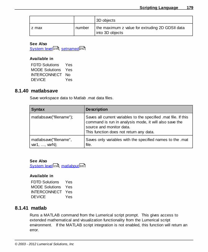
Scripting Language 179
© 2003 - 2012 Lumerical Solutions, Inc
3D objects
z max number the maximum z value for extruding 2D GDSII datainto 3D objects
See AlsoSystem level , setnamed
Available in
FDTD SolutionsMODE SolutionsINTERCONNECTDEVICE
YesYesNoYes
8.1.40 matlabsave
Save workspace data to Matlab .mat data files.
Syntax Description
matlabsave("filename"); Saves all current variables to the specified .mat file. If thiscommand is run in analysis mode, it will also save thesource and monitor data.This function does not return any data.
matlabsave("filename",var1, ..., varN);
Saves only variables with the specified names to the .matfile.
See Also System level , matlabput
Available in
FDTD SolutionsMODE SolutionsINTERCONNECTDEVICE
YesYesYesYes
8.1.41 matlab
Runs a MATLAB command from the Lumerical script prompt. This gives access toextended mathematical and visualization functionality from the Lumerical scriptenvironment. If the MATLAB script integration is not enabled, this function will return anerror.
156 292
156 181

Reference Guide180
© 2003 - 2012 Lumerical Solutions, Inc
The first time a MATLAB function (matlab, matlabget or matlabput) is called, a MATLABsession will be started and a connection will be established with the Lumerical scriptingenvironment. Once this connection is established, MATLAB commands can be run usingthe matlab function. It is important to understand that the MATLAB and the Lumericalscript variable workspaces are completely separate and independent. A MATLABcommand cannot act on a variable defined in the Lumerical workspace, and vice-versa. Variables must be passed between the workspaces using the matlabget and matlabputfunctions. At any time you may examine the MATLAB workspace or interact with theMATLAB environment by typing commands at the MATLAB script prompt.
The output from the MATLAB commands will be printed at the Lumerical script prompt.One limitation of the matlab function is that no error reporting is provided to either theLumerical script prompt or the MATLAB prompt. MATLAB commands should be tested bytyping them directly into the MATLAB prompt before they are called from a Lumericalscript.
When you have a long sequence of MATLAB commands, you may find it more convenientto save them in a MATLAB m-file. Then, you can simply call the m-file by running a singlecommand.
Setup instructions and system requirements for the MATLAB script integration featurecan be found in the online Knowledge Base. See the Setup and Configuration section ofthe Installation Guide.
Syntax Description
matlab("command"); command: a string containing one or more valid MATLABcommands.
matlab(" command_1 command_2");
Multi-line strings can be used in script files to contain ablock of MATLAB commands. Multi-line strings are notsupported at the script command prompt.
See AlsoSystem level , matlabget , matlabput
Available in
156 181 181
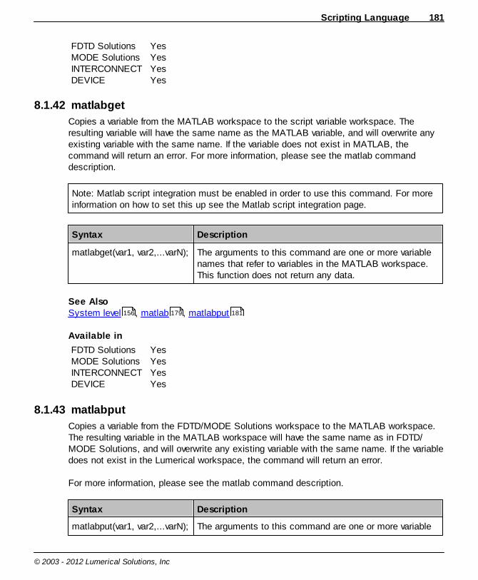
Scripting Language 181
© 2003 - 2012 Lumerical Solutions, Inc
FDTD SolutionsMODE SolutionsINTERCONNECTDEVICE
YesYesYesYes
8.1.42 matlabget
Copies a variable from the MATLAB workspace to the script variable workspace. Theresulting variable will have the same name as the MATLAB variable, and will overwrite anyexisting variable with the same name. If the variable does not exist in MATLAB, thecommand will return an error. For more information, please see the matlab commanddescription.
Note: Matlab script integration must be enabled in order to use this command. For moreinformation on how to set this up see the Matlab script integration page.
Syntax Description
matlabget(var1, var2,...varN); The arguments to this command are one or more variablenames that refer to variables in the MATLAB workspace.This function does not return any data.
See AlsoSystem level , matlab , matlabput
Available in
FDTD SolutionsMODE SolutionsINTERCONNECTDEVICE
YesYesYesYes
8.1.43 matlabput
Copies a variable from the FDTD/MODE Solutions workspace to the MATLAB workspace.The resulting variable in the MATLAB workspace will have the same name as in FDTD/MODE Solutions, and will overwrite any existing variable with the same name. If the variabledoes not exist in the Lumerical workspace, the command will return an error.
For more information, please see the matlab command description.
Syntax Description
matlabput(var1, var2,...varN); The arguments to this command are one or more variable
156 179 181
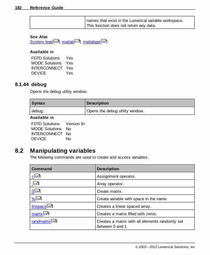
Reference Guide182
© 2003 - 2012 Lumerical Solutions, Inc
names that exist in the Lumerical variable workspace.This function does not return any data.
See AlsoSystem level , matlab , matlabget
Available in
FDTD SolutionsMODE SolutionsINTERCONNECTDEVICE
YesYesYesYes
8.1.44 debug
Opens the debug utility window.
Syntax Description
debug; Opens the debug utility window.
Available in
FDTD SolutionsMODE SolutionsINTERCONNECTDEVICE
Version 8+NoNoNo
8.2 Manipulating variablesThe following commands are used to create and access variables.
Command Description
= Assignment operator.
: Array operator.
[] Create matrix.
% Create variable with space in the name
linspace Creates a linear spaced array.
matrix Creates a matrix filled with zeros.
randmatrix Creates a matrix with all elements randomly setbetween 0 and 1
156 179 181
183
183
184
184
185
185
186
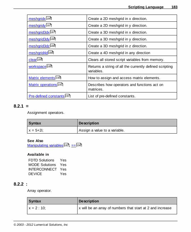
Scripting Language 183
© 2003 - 2012 Lumerical Solutions, Inc
meshgridx Create a 2D meshgrid in x direction.
meshgridy Create a 2D meshgrid in y direction.
meshgrid3dx Create a 3D meshgrid in x direction.
meshgrid3dy Create a 3D meshgrid in y direction.
meshgrid3dz Create a 3D meshgrid in z direction.
meshgrid4d Create a 4D meshgrid in any direction
clear Clears all stored script variables from memory.
workspace Returns a string of all the currently defined scriptingvariables.
Matrix elements How to assign and access matrix elements.
Matrix operations Describes how operators and functions act onmatrices.
Pre-defined constants List of pre-defined constants.
8.2.1 =
Assignment operators.
Syntax Description
x = 5+2i; Assign a value to a variable.
See AlsoManipulating variables , ==
Available in
FDTD SolutionsMODE SolutionsINTERCONNECTDEVICE
YesYesYesYes
8.2.2 :
Array operator.
Syntax Description
x = 2 : 10; x will be an array of numbers that start at 2 and increase
186
187
187
188
188
188
189
189
190
191
191
182 196
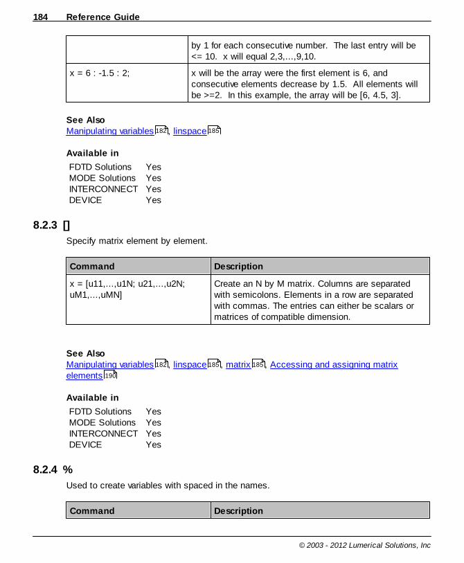
Reference Guide184
© 2003 - 2012 Lumerical Solutions, Inc
by 1 for each consecutive number. The last entry will be<= 10. x will equal 2,3,...,9,10.
x = 6 : -1.5 : 2; x will be the array were the first element is 6, andconsecutive elements decrease by 1.5. All elements willbe >=2. In this example, the array will be [6, 4.5, 3].
See AlsoManipulating variables , linspace
Available in
FDTD SolutionsMODE SolutionsINTERCONNECTDEVICE
YesYesYesYes
8.2.3 []
Specify matrix element by element.
Command Description
x = [u11,...,u1N; u21,...,u2N;uM1,...,uMN]
Create an N by M matrix. Columns are separatedwith semicolons. Elements in a row are separatedwith commas. The entries can either be scalars ormatrices of compatible dimension.
See AlsoManipulating variables , linspace , matrix , Accessing and assigning matrixelements
Available in
FDTD SolutionsMODE SolutionsINTERCONNECTDEVICE
YesYesYesYes
8.2.4 %
Used to create variables with spaced in the names.
Command Description
182 185
182 185 185
190

Scripting Language 185
© 2003 - 2012 Lumerical Solutions, Inc
%variable with space% To create a variable name that contains spaces,such as "variable with space", put a percentage signbefore and after the variable name.
See AlsoManipulating variables
Available in
FDTD SolutionsMODE SolutionsINTERCONNECTDEVICE
YesYesYesYes
8.2.5 linspace
Creates a linearly spaced array.
Syntax Description
x = linspace(min,max,num); x will be an array with num elements, linearly spacedbetween min and max. If num is set to 1, then x will be theaverage of min and max.
See AlsoManipulating variables , : , []
Available in
FDTD SolutionsMODE SolutionsINTERCONNECTDEVICE
YesYesYesYes
8.2.6 matrix
Initialize a matrix. All elements are set to zero.
Syntax Description
x = matrix(i,j,k,....); Initializes an i x j x k x .... matrix.
See AlsoManipulating variables , linspace , []
182
182 183 184
182 185 184
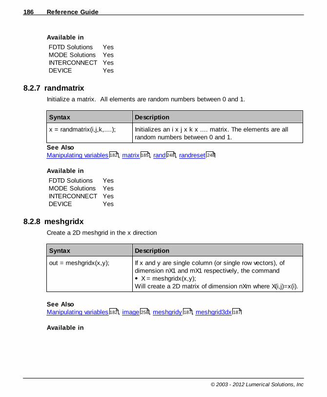
Reference Guide186
© 2003 - 2012 Lumerical Solutions, Inc
Available in
FDTD SolutionsMODE SolutionsINTERCONNECTDEVICE
YesYesYesYes
8.2.7 randmatrix
Initialize a matrix. All elements are random numbers between 0 and 1.
Syntax Description
x = randmatrix(i,j,k,....); Initializes an i x j x k x .... matrix. The elements are allrandom numbers between 0 and 1.
See AlsoManipulating variables , matrix , rand , randreset
Available in
FDTD SolutionsMODE SolutionsINTERCONNECTDEVICE
YesYesYesYes
8.2.8 meshgridx
Create a 2D meshgrid in the x direction
Syntax Description
out = meshgridx(x,y); If x and y are single column (or single row vectors), ofdimension nX1 and mX1 respectively, the command
X = meshgridx(x,y); Will create a 2D matrix of dimension nXm where X(i,j)=x(i).
See AlsoManipulating variables , image , meshgridy , meshgrid3dx
Available in
182 185 248 248
182 258 187 187

Scripting Language 187
© 2003 - 2012 Lumerical Solutions, Inc
FDTD SolutionsMODE SolutionsINTERCONNECTDEVICE
YesYesYesYes
8.2.9 meshgridy
Create a 2D meshgrid in the y direction
Syntax Description
out = meshgridy(x,y); If x and y are single column (or single row vectors), ofdimension nX1 and mX1 respectively, the command
Y = meshgridy(x,y); Will create a 2D matrix of dimension nXm where Y(i,j)=y(j).
See AlsoManipulating variables , image , meshgridx , meshgrid3dx
Available in
FDTD SolutionsMODE SolutionsINTERCONNECTDEVICE
YesYesYesYes
8.2.10 meshgrid3dx
Create a 3D meshgrid in the x direction
Syntax Description
out = meshgrid3dx(x,y,z); The 3D version of meshgridx and meshgridy.
See AlsoManipulating variables , meshgridx , meshgridy , meshgrid3dy , meshgrid3dz
Available in
FDTD SolutionsMODE SolutionsINTERCONNECTDEVICE
YesYesYesYes
182 258 186 187
182 186 187 188 188
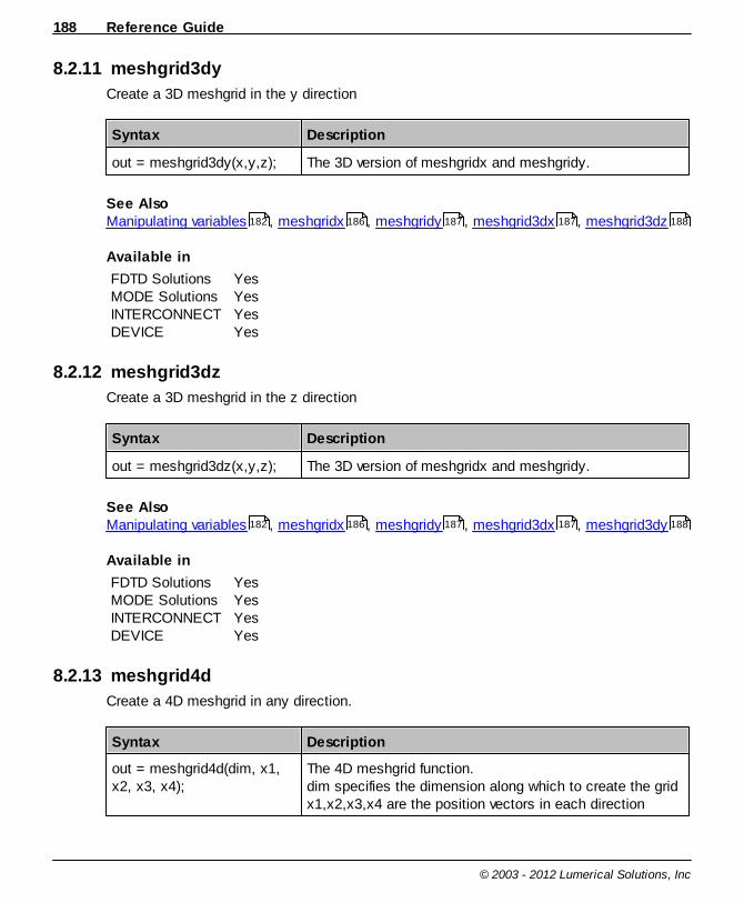
Reference Guide188
© 2003 - 2012 Lumerical Solutions, Inc
8.2.11 meshgrid3dy
Create a 3D meshgrid in the y direction
Syntax Description
out = meshgrid3dy(x,y,z); The 3D version of meshgridx and meshgridy.
See AlsoManipulating variables , meshgridx , meshgridy , meshgrid3dx , meshgrid3dz
Available in
FDTD SolutionsMODE SolutionsINTERCONNECTDEVICE
YesYesYesYes
8.2.12 meshgrid3dz
Create a 3D meshgrid in the z direction
Syntax Description
out = meshgrid3dz(x,y,z); The 3D version of meshgridx and meshgridy.
See AlsoManipulating variables , meshgridx , meshgridy , meshgrid3dx , meshgrid3dy
Available in
FDTD SolutionsMODE SolutionsINTERCONNECTDEVICE
YesYesYesYes
8.2.13 meshgrid4d
Create a 4D meshgrid in any direction.
Syntax Description
out = meshgrid4d(dim, x1,x2, x3, x4);
The 4D meshgrid function. dim specifies the dimension along which to create the gridx1,x2,x3,x4 are the position vectors in each direction
182 186 187 187 188
182 186 187 187 188

Scripting Language 189
© 2003 - 2012 Lumerical Solutions, Inc
See AlsoManipulating variables , meshgridx , meshgridy , meshgrid3dy , meshgrid3dz
Available in
FDTD SolutionsMODE SolutionsINTERCONNECTDEVICE
YesYesYesYes
8.2.14 clear
Clears all stored workspace variables. This will not clear any simulation data stored in d-cards. The variables c, pi, eps0, mu0 will be reset to their default values.
Syntax Description
clear; Clears all workspace variables.This function does not return any data.
See AlsoManipulating variables , cleardcard
Available in
FDTD SolutionsMODE SolutionsINTERCONNECTDEVICE
YesYesYesYes
8.2.15 workspace
Returns a list of all the currently defined variables in the scripting workspace.
Syntax Description
out = workspace; Returns a string that lists all currently defined variables inthe workspace.Use ?workspace; to print this to the screen.
See AlsoManipulating variables
Available in
182 186 187 188 188
182 353
182

Reference Guide190
© 2003 - 2012 Lumerical Solutions, Inc
FDTD SolutionsMODE SolutionsINTERCONNECTDEVICE
YesYesYesYes
8.2.16 Accessing and assigning matrix elements
Accessing and assigning matrix elements.
The square brackets method of defining matrices is only available in FDTD solutions.
Command Description
x = [u; v; w] Create a column vector. u,v,w can either be scalarsor matrices of compatible dimension.
x = [u, v, w] Create a row vector. u,v,w can either be scalars ormatrices of compatible dimension.
x(7) = 5; Set the 7th element of x to 5.
x(7) = y(2); Set the 7th element of x to the 2nd element of y.
x(3,1,8) = 3; Set an element of a multidimensional matrix to 3.
x(2:5,1) = 1:4; Set a sub-matrix of x to values 1:4. In theassignment A(I,...) = B, if B is not a scalar, the sub-matrix A(I,...) must be the same same size as B. If Bis a scalar, then all the values of the sub-matrix areset to B.
x(2:5,1) = 1; Set all the values in a sub-matrix of x to 1.
x = y(1:10,2,1:20); x is equal to a sub-matrix of y.
x = matrix(2,3);x(4)=7;
Multi-dimension matrices can be accessed with asingle index.
x=y(z); Indices stored in matrix (z) used to select elementsof matrix y. length(x) will equal length(z).
See AlsoManipulating variables
Available in
182

Scripting Language 191
© 2003 - 2012 Lumerical Solutions, Inc
FDTD SolutionsMODE SolutionsINTERCONNECTDEVICE
YesYesYesYes
8.2.17 Matrix operators
Almost all the scripting functions will act element by element on matrices. Single numbersare treated as matrices of dimension 1x1. The following table provides some examples.
Dimension ofx
Dimension ofy
Operation Dimension ofz
Value of z
1x1 N/A z = sin(x) 1x1 z11
= sin(x11
)
1x1 1x1 z = x * y 1x1 z11
= x11
* y11
10x10 1x1 z = x * y 10x10 Zij = x
ij * y
11
10x10 10x10 z = x * y 10x10 Zij = x
ij * y
ij
10x10 11x11 z = x * y Error Error
See AlsoManipulating variables
Available in
FDTD SolutionsMODE SolutionsINTERCONNECTDEVICE
YesYesYesYes
8.2.18 Pre-defined constants
Name Description
pi The number .
c The speed of light in a vacuum in m/s.
eps0 The permittivity of free space in SI units.
mu0 The permeability of free space in SI units.
h The Planck constant.
182

Reference Guide192
© 2003 - 2012 Lumerical Solutions, Inc
hbar The reduced Planck constant.
true Logical TRUE (1).
false Logical FALSE (0);
e The electron volt.
See AlsoManipulating variables
Available in
FDTD SolutionsMODE SolutionsINTERCONNECTDEVICE
YesYesYesYes
8.3 OperatorsStandard mathematical and string operators.
Algebraic operators
Command Description
* Multiplication. Ex: y = x * z;
/ Division. Ex: y = x / z;
+ Addition. Ex: y = x + z;
- Subtraction. Ex: y = x – z;
- Negative. Ex: y = -x;
^ Power. Ex: y = x 3;In expression A^B, if B is complex, the phase of A isevaluated from - to .
Logical and relational operators
Command Description
== Comparison.
almostequal Almost equal comparison operator.
!= Not equal.
<= Less than or equal to.
182
194
194
195
195
195
196
196
196
197
198
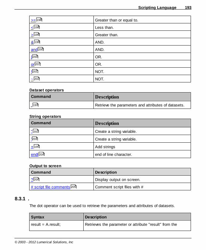
Scripting Language 193
© 2003 - 2012 Lumerical Solutions, Inc
>= Greater than or equal to.
< Less than.
> Greater than.
& AND.
and AND.
| OR.
or OR.
! NOT.
~ NOT.
Dataset operators
Command Description
. Retrieve the parameters and attributes of datasets.
String operators
Command Description
" Create a string variable.
' Create a string variable.
+ Add strings
endl end of line character.
Output to screen
Command Description
? Display output on screen.
# script file comments Comment script files with #
8.3.1 .
The dot operator can be used to retrieve the parameters and attributes of datasets.
Syntax Description
result = A.result; Retrieves the parameter or attribute "result" from the
198
198
199
199
200
200
201
201
202
193
202
203
195
204
204
205
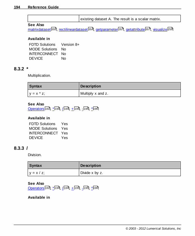
Reference Guide194
© 2003 - 2012 Lumerical Solutions, Inc
existing dataset A. The result is a scalar matrix.
See Alsomatrixdataset , rectilineardataset , getparameter , getattribute , visualize
Available in
FDTD SolutionsMODE SolutionsINTERCONNECTDEVICE
Version 8+NoNoNo
8.3.2 *
Multiplication.
Syntax Description
y = x * z; Multiply x and z.
See AlsoOperators , * , / , + , - , ^
Available in
FDTD SolutionsMODE SolutionsINTERCONNECTDEVICE
YesYesYesYes
8.3.3 /
Division.
Syntax Description
y = x / z; Divide x by z.
See AlsoOperators , * , / , + , - , ^
Available in
355 354 357 357 259
192 194 194 195 195 196
192 194 194 195 195 196
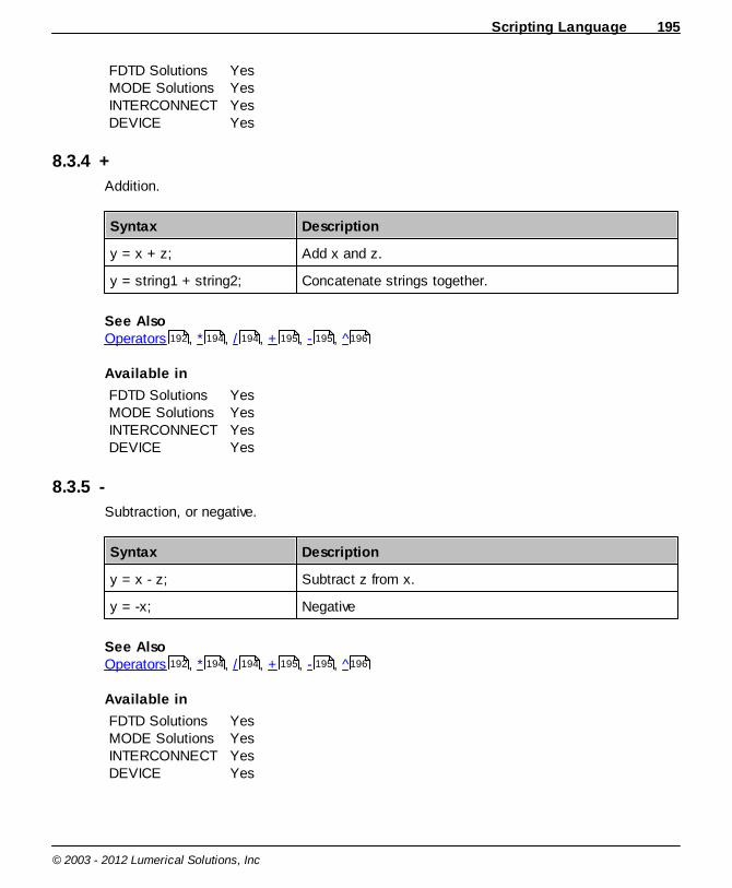
Scripting Language 195
© 2003 - 2012 Lumerical Solutions, Inc
FDTD SolutionsMODE SolutionsINTERCONNECTDEVICE
YesYesYesYes
8.3.4 +
Addition.
Syntax Description
y = x + z; Add x and z.
y = string1 + string2; Concatenate strings together.
See AlsoOperators , * , / , + , - , ^
Available in
FDTD SolutionsMODE SolutionsINTERCONNECTDEVICE
YesYesYesYes
8.3.5 -
Subtraction, or negative.
Syntax Description
y = x - z; Subtract z from x.
y = -x; Negative
See AlsoOperators , * , / , + , - , ^
Available in
FDTD SolutionsMODE SolutionsINTERCONNECTDEVICE
YesYesYesYes
192 194 194 195 195 196
192 194 194 195 195 196

Reference Guide196
© 2003 - 2012 Lumerical Solutions, Inc
8.3.6 ^
Power. In expression A^B, if B is complex, the phase of A is evaluated from - to .
Syntax Description
y = x 3; x cubed.
See Also Operators , * , / , + , - , ^
Available in
FDTD SolutionsMODE SolutionsINTERCONNECTDEVICE
YesYesYesYes
8.3.7 ==
Logical comparison. This operators can be used with complex numbers and strings.
Syntax Description
out = y == x; Returns 1 if x and y are equal. Returns 0 otherwise.
See AlsoOperators , = , almostequal , != , <= , >= , < , > , & , and , |, or , ! , ~
Available in
FDTD SolutionsMODE SolutionsINTERCONNECTDEVICE
YesYesYesYes
8.3.8 almostequal
Almost equal comparison operator. When using floating point numbers (rather thanintegers), two values that are meant to be equal may not be exactly equal due to roundingerrors that are always present in floating point calculations. In such cases, the almostequal function can be useful.
Syntax Description
192 194 194 195 195 196
192 183 196 197 198 198 198 199 199 200 200
201 201 202
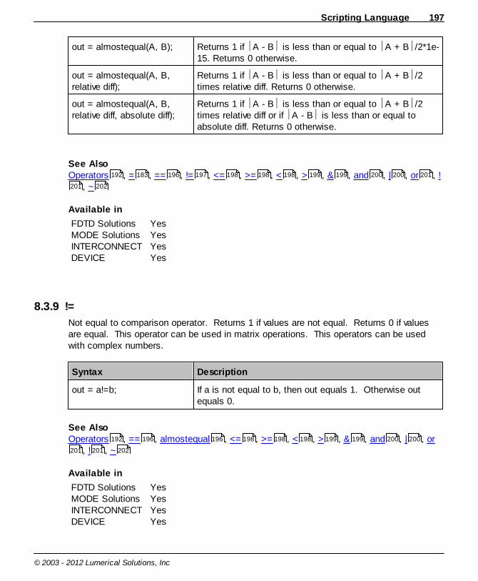
Scripting Language 197
© 2003 - 2012 Lumerical Solutions, Inc
out = almostequal(A, B); Returns 1 if A - B is less than or equal to A + B /2*1e-15. Returns 0 otherwise.
out = almostequal(A, B,relative diff);
Returns 1 if A - B is less than or equal to A + B /2times relative diff. Returns 0 otherwise.
out = almostequal(A, B,relative diff, absolute diff);
Returns 1 if A - B is less than or equal to A + B /2times relative diff or if A - B is less than or equal toabsolute diff. Returns 0 otherwise.
See AlsoOperators , = , == , != , <= , >= , < , > , & , and , | , or , !
, ~
Available in
FDTD SolutionsMODE SolutionsINTERCONNECTDEVICE
YesYesYesYes
8.3.9 !=
Not equal to comparison operator. Returns 1 if values are not equal. Returns 0 if valuesare equal. This operator can be used in matrix operations. This operators can be usedwith complex numbers.
Syntax Description
out = a!=b; If a is not equal to b, then out equals 1. Otherwise outequals 0.
See AlsoOperators , == , almostequal , <= , >= , < , > , & , and , | , or
, ! , ~
Available in
FDTD SolutionsMODE SolutionsINTERCONNECTDEVICE
YesYesYesYes
192 183 196 197 198 198 198 199 199 200 200 201
201 202
192 196 196 198 198 198 199 199 200 200
201 201 202
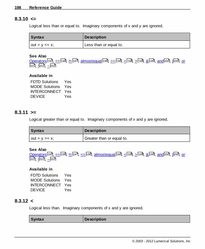
Reference Guide198
© 2003 - 2012 Lumerical Solutions, Inc
8.3.10 <=
Logical less than or equal to. Imaginary components of x and y are ignored.
Syntax Description
out = y <= x; Less than or equal to.
See AlsoOperators , == , != , almostequal , >= , < , > , & , and , | , or
, ! , ~
Available in
FDTD SolutionsMODE SolutionsINTERCONNECTDEVICE
YesYesYesYes
8.3.11 >=
Logical greater than or equal to. Imaginary components of x and y are ignored.
Syntax Description
out = y >= x; Greater than or equal to.
See AlsoOperators , == , != , <= , almostequal , < , > , & , and , | , or
, ! , ~
Available in
FDTD SolutionsMODE SolutionsINTERCONNECTDEVICE
YesYesYesYes
8.3.12 <
Logical less than. Imaginary components of x and y are ignored.
Syntax Description
192 196 197 196 198 198 199 199 200 200
201 201 202
192 196 197 198 196 198 199 199 200 200
201 201 202
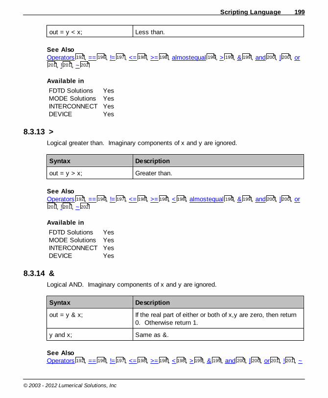
Scripting Language 199
© 2003 - 2012 Lumerical Solutions, Inc
out = y < x; Less than.
See AlsoOperators , == , != , <= , >= , almostequal , > , & , and , | , or
, ! , ~
Available in
FDTD SolutionsMODE SolutionsINTERCONNECTDEVICE
YesYesYesYes
8.3.13 >
Logical greater than. Imaginary components of x and y are ignored.
Syntax Description
out = y > x; Greater than.
See AlsoOperators , == , != , <= , >= , < , almostequal , & , and , | , or
, ! , ~
Available in
FDTD SolutionsMODE SolutionsINTERCONNECTDEVICE
YesYesYesYes
8.3.14 &
Logical AND. Imaginary components of x and y are ignored.
Syntax Description
out = y & x; If the real part of either or both of x,y are zero, then return0. Otherwise return 1.
y and x; Same as &.
See AlsoOperators , == , != , <= , >= , < , > , & , and , | , or , ! , ~
192 196 197 198 198 196 199 199 200 200
201 201 202
192 196 197 198 198 198 196 199 200 200
201 201 202
192 196 197 198 198 198 199 199 200 200 201 201

Reference Guide200
© 2003 - 2012 Lumerical Solutions, Inc
Available in
FDTD SolutionsMODE SolutionsINTERCONNECTDEVICE
YesYesYesYes
8.3.15 and
Logical AND. Imaginary components of x and y are ignored.
Syntax Description
out = y & x; If the real part of either or both of x,y are zero, then return0. Otherwise return 1.
y and x; Same as &.
See AlsoOperators , == , != , <= , >= , < , > , & , and , | , or , ! , ~
Available in
FDTD SolutionsMODE SolutionsINTERCONNECTDEVICE
YesYesYesYes
8.3.16 |
Logical OR. Imaginary components of x and y are ignored.
Syntax Description
out = y | x; If the real part of either or both of x,y is non-zero, thenreturn 1. Otherwise return 0.
y or x; Same as |.
See AlsoOperators , == , != , <= , >= , < , > , & , and , | , or , ! , ~
202
192 196 197 198 198 198 199 199 200 200 201 201
202
192 196 197 198 198 198 199 199 200 200 201 201
202
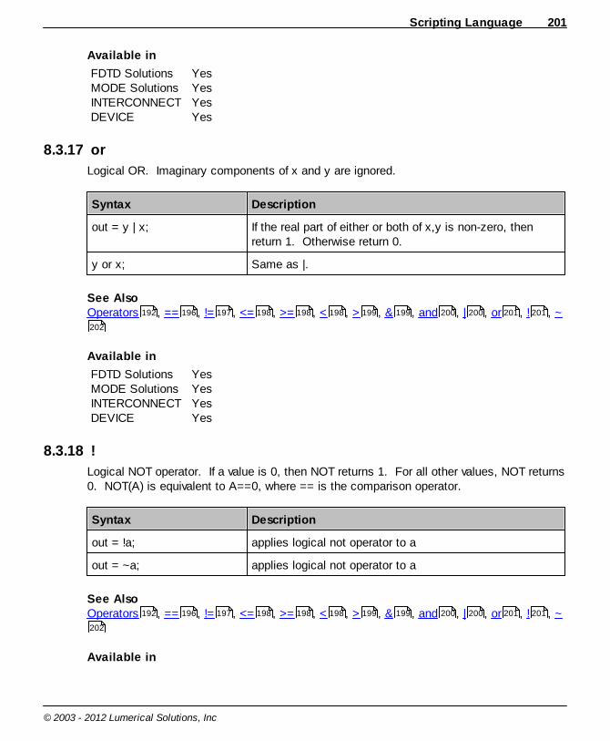
Scripting Language 201
© 2003 - 2012 Lumerical Solutions, Inc
Available in
FDTD SolutionsMODE SolutionsINTERCONNECTDEVICE
YesYesYesYes
8.3.17 or
Logical OR. Imaginary components of x and y are ignored.
Syntax Description
out = y | x; If the real part of either or both of x,y is non-zero, thenreturn 1. Otherwise return 0.
y or x; Same as |.
See AlsoOperators , == , != , <= , >= , < , > , & , and , | , or , ! , ~
Available in
FDTD SolutionsMODE SolutionsINTERCONNECTDEVICE
YesYesYesYes
8.3.18 !
Logical NOT operator. If a value is 0, then NOT returns 1. For all other values, NOT returns0. NOT(A) is equivalent to A==0, where == is the comparison operator.
Syntax Description
out = !a; applies logical not operator to a
out = ~a; applies logical not operator to a
See AlsoOperators , == , != , <= , >= , < , > , & , and , | , or , ! , ~
Available in
192 196 197 198 198 198 199 199 200 200 201 201
202
192 196 197 198 198 198 199 199 200 200 201 201
202

Reference Guide202
© 2003 - 2012 Lumerical Solutions, Inc
FDTD SolutionsMODE SolutionsINTERCONNECTDEVICE
YesYesYesYes
8.3.19 ~
Logical NOT operator. If a value is 0, then NOT returns 1. For all other values, NOT returns0. NOT(A) is equivalent to A==0, where == is the comparison operator.
Syntax Description
out = !a; applies logical not operator to a
out = ~a; applies logical not operator to a
See AlsoOperators , == , != , <= , >= , < , > , & , and , | , or , ! , ~
Available in
FDTD SolutionsMODE SolutionsINTERCONNECTDEVICE
YesYesYesYes
8.3.20 "
String operator. Strings can be created with single or double quotes.
The following escape sequences are recognized when creating strings with double quotes:\" double quotes in string\n newline (linefeed) character in string\\ backslash in string
Syntax Description
out="my string"; use double quotes to create strings
NOTE: Literal backslashes and double quotesIt is always possible to create a literal backslash in a string with \\. However, \ alsoresults in a literal backslash, IF it it will not be interpreted as part of an escape sequence(\n, \", \\). This note is important when storing paths in strings.
192 196 197 198 198 198 199 199 200 200 201 201
202
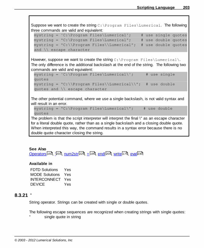
Scripting Language 203
© 2003 - 2012 Lumerical Solutions, Inc
Suppose we want to create the string C:\Program Files\Lumerical. The following
three commands are valid and equivalent:mystring = 'C:\Program Files\Lumerical'; # use single quotesmystring = "C:\Program Files\Lumerical"; # use double quotesmystring = "C:\\Program Files\\Lumerical"; # use double quotesand \\ escape character
However, suppose we want to create the string C:\Program Files\Lumerical\.
The only difference is the additional backslash at the end of the string. The following twocommands are valid and equivalent:mystring = 'C:\Program Files\Lumerical\'; # use singlequotesmystring = "C:\\Program Files\\Lumerical\\"; # use doublequotes and \\ escape character
The other potential command, where we use a single backslash, is not valid syntax andwill result in an error.mystring = "C:\Program Files\Lumerical\"; # use doublequotes
The problem is that the script interpreter will interpret the final \" as an escape characterfor a literal double quote, rather than as a single backslash and a closing double quote. When interpreted this way, the command results in a syntax error because there is nodouble quote character closing the string.
See AlsoOperators , ' , num2str , + , endl , write , eval
Available in
FDTD SolutionsMODE SolutionsINTERCONNECTDEVICE
YesYesYesYes
8.3.21 '
String operator. Strings can be created with single or double quotes.
The following escape sequences are recognized when creating strings with single quotes:'' single quote in string
192 203 229 195 204 175 230

Reference Guide204
© 2003 - 2012 Lumerical Solutions, Inc
Syntax Description
out='my string'; use single quotes to create strings
See AlsoOperators , " , num2str , + , endl , write , eval
Available in
FDTD SolutionsMODE SolutionsINTERCONNECTDEVICE
YesYesYesYes
8.3.22 endl
Add an end of line character to a string
Syntax Description
out = "line1"+endl+"line2"; Add an end of line character to the string.
See AlsoOperators , num2str , + , " , write
Available in
FDTD SolutionsMODE SolutionsINTERCONNECTDEVICE
YesYesYesYes
8.3.23 ?
Print output to the screen. Use the format script command to change the precision of theoutput.
Syntax Description
?command; Displays the output of the command on the screenThis function does not return any data.
See AlsoSystem level , write , format , #
192 202 229 195 204 175 230
192 229 195 202 175
156 175 173 205
Scripting Language 205
© 2003 - 2012 Lumerical Solutions, Inc
Available in
FDTD SolutionsMODE SolutionsINTERCONNECTDEVICE
YesYesYesYes
8.3.24 comments
Use the # character to comment script files. Anything after the # character is ignored. Thecomments are not displayed when the script file is run. Comments can not be used whentyping commands directly into the script prompt.
Syntax Description
x=1; # set x to 1 Anything after the # character is ignored.
See AlsoSystem level
Available in
FDTD SolutionsMODE SolutionsINTERCONNECTDEVICE
YesYesYesYes
8.4 FunctionsStandard mathematical and matrix functions.
Trigonometric and complex
Command Description
sin Trigonometric sin function.
cos Trigonometric cos function.
tan Trigonometric tan function.
asin Inverse trigonometric sin function.
acos Inverse trigonometric cos function.
atan Inverse trigonometric tan function.
atan2 Same as atan, but returns angle in correct quadrant.
156
209
209
210
210
211
211
212

Reference Guide206
© 2003 - 2012 Lumerical Solutions, Inc
real Returns the real part of variable
imag Returns the imaginary part of variable
conj Complex conjugate
abs Absolute value
angle Phase of a complex number.
unwrap Removes phase difference of more than 2
Logarithmic, exponential and power
Command Description
log The natural logarithm. Input can be complex ornegative.
log10 The log, base 10. Input can be complex or negative.
sqrt The square root.
exp The exponential.
Matrix functions
Command Description
size Returns the dimensions of a matrix.
length Returns the total number of elements in a matrix.
pinch Remove singleton dimensions from a matrix.
sum The sum of a matrix.
max The max value in a matrix.
min The min value in a matrix.
dot The dot product of two vectors.
cross The cross product of two vectors.
flip Flip a matrix in one dimension.
interp Linear interpolation function.
spline Cubic spline interpolation.
integrate Integrate a matrix.
integrate2 Integrate a matrix, ignore singleton dimensions.
212
212
213
213
214
214
215
215
215
216
216
217
217
218
218
219
219
220
222
224
225
225
226
Scripting Language 207
© 2003 - 2012 Lumerical Solutions, Inc
find Find values that satisfy a condition in a matrix.
findpeaks Find peaks in a matrix.
transpose Transpose a matrix.
ctranspose Transpose a matrix, and do complex conjugate.
mult Perform matrix multiplication of two or morematrices.
reshape Reshape the matrix to have different dimensionsconserving the overall product of the dimensions.
eig Calculate the eigenvalues and/or eigenvectors of amatrix.
permute Rearrange the dimensions of a matrix.
inv Calculate the inverse of a matrix.
See alsoManipulating variables
String functions
Command Description
num2str Convert number to a string.
str2num Convert a string into a floating point number.
eval Execute string containing Lumerical scriptinglanguage.
feval Run a Lumerical script file.
length Returns the total length of the string.
substring Returns a substring of a string, as a specifiedposition and length.
findstring Returns the position of a substring in a string.
replace Replaces a part of a string with another, at aspecified position.
replacestring Replaces all instances of a substring with anotherstring.
Frequency and time-domain
227
228
228
229
221
223
220
222
223
182
229
230
230
231
217
231
232
232
233

Reference Guide208
© 2003 - 2012 Lumerical Solutions, Inc
Command Description
fft Fast Fourier transform.
fftw Returns the angular frequency vector.
fftk Returns the spatial wavevector kx.
invfft Inverse fft.
czt Chirped z-transform.
Line and polygon functions
Command Description
polyarea Returns the area of a polygon.
centroid Returns the center of mass of a polygon.
polyintersect Determines if two polygons intersect.
inpoly Determines if a series of points are inside our outsidea polygon.
polygrow Grows or shrinks a polygon by a specified amount.
polyand Combines two polygons into one with an andoperation.
polyor Combines two polygons into one with an oroperation.
polyxor Combines two polygons into one with a xoroperation.
lineintersect Returns the intersection of line segments.
linecross Determines if line segments cross each other.
Miscellaneous
Command Description
ceil Round up.
floor Round down.
mod Modulus after division.
round Rounds to the nearest integer.
rand Returns a uniformly distributed random number
233
235
236
237
238
239
240
240
241
241
242
242
244
244
245
246
246
246
247
248
Scripting Language 209
© 2003 - 2012 Lumerical Solutions, Inc
between 0 and 1.
randreset Resets the random number seed.
finite Determines if a number is finite or NaN.
solar Returns the solar power spectrum
stackrt Calculates reflection and transmission of multi-layerstacks
8.4.1 sin
Trigonometric sine function. Angle units are in radians. Function is defined for complexangles. Phase of a complex number is evaluated between - and .
Syntax Description
out = sin(x); Returns the complex sine of x.
See Also Functions , asin
Available in
FDTD SolutionsMODE SolutionsINTERCONNECTDEVICE
YesYesYesYes
8.4.2 cos
Trigonometric cosine function. Angle units are in radians. Function is defined for complexangles. Phase of a complex number is evaluated between - and .
Syntax Description
out = cos(x); Returns the complex cosine of x.
See Also Functions , acos
Available in
248
249
249
250
205 210
205 211
Reference Guide210
© 2003 - 2012 Lumerical Solutions, Inc
FDTD SolutionsMODE SolutionsINTERCONNECTDEVICE
YesYesYesYes
8.4.3 tan
Trigonometric tangent function. Angle units are in radians. Function is defined for complexangles. Phase of a complex number is evaluated between - and .
Syntax Description
out = tan(x); Returns the complex tangent of x.
See Also Functions , atan , atan2
Available in
FDTD SolutionsMODE SolutionsINTERCONNECTDEVICE
YesYesYesYes
8.4.4 asin
Inverse trigonometric sine function. Angle units are in radians. Function is defined forcomplex values. Phase of a complex number is evaluated between - and . If x iscomplex, or abs(x) > 1, the following equation is used: asin(x) = -i ln( ix + sqrt(1-x 2))
Syntax Description
out = asin(x); Returns the complex arcsine of x.
See Also Functions , sin
Available in
FDTD SolutionsMODE SolutionsINTERCONNECTDEVICE
YesYesYesYes
205 211 212
205 209
Scripting Language 211
© 2003 - 2012 Lumerical Solutions, Inc
8.4.5 acos
Inverse trigonometric cosine function. Angle units are in radians. Function is defined forcomplex values. Phase of a complex number is evaluated between - and . If x iscomplex, or abs(x) > 1, the following equation is used: acos(x) = -i ln( x + i sqrt( 1-x 2))
Syntax Description
out = acos(x); Returns the complex arccosine of x.
See Also Functions , cos
Available in
FDTD SolutionsMODE SolutionsINTERCONNECTDEVICE
YesYesYesYes
8.4.6 atan
Inverse trigonometric tangent function. Angle units are in radians. Function is defined forcomplex values. Phase of a complex number is evaluated between - and . If x iscomplex, or abs(x) > 1, the following equation is used: atan(x) = 0.5 i ln( (i+x)/(i-x) )
Syntax Description
out = atan(x); Returns the complex arctangent of x.
See Also Functions , atan2 , tan
Available in
FDTD SolutionsMODE SolutionsINTERCONNECTDEVICE
YesYesYesYes
205 209
205 212 210

Reference Guide212
© 2003 - 2012 Lumerical Solutions, Inc
8.4.7 atan2
Inverse trigonometric tangent function, calculates the arctangent of y/x, but returns theangle in the correct quadrant. Angle units are in radians. Function is defined for realvalues only.
Syntax Description
out = atan2(y,x); x,y must be real.
See Also Functions , atan , tan
Available in
FDTD SolutionsMODE SolutionsINTERCONNECTDEVICE
YesYesYesYes
8.4.8 real
Returns the real part of a number or matrix.
Syntax Description
out = real(x); Returns the real part of x.
See Also Functions , imag
Available in
FDTD SolutionsMODE SolutionsINTERCONNECTDEVICE
YesYesYesYes
8.4.9 imag
Returns the imaginary part of a number or matrix.
Syntax Description
out = imag(x); Returns the imaginary part of x.
205 211 210
205 212

Scripting Language 213
© 2003 - 2012 Lumerical Solutions, Inc
See Also Functions , real , conj
Available in
FDTD SolutionsMODE SolutionsINTERCONNECTDEVICE
YesYesYesYes
8.4.10 conj
Returns the complex conjugate of a number or matrix.
Syntax Description
out = conj(x); Returns the complex conjugate of x.
See Also Functions , real , imag
Available in
FDTD SolutionsMODE SolutionsINTERCONNECTDEVICE
YesYesYesYes
8.4.11 abs
Returns the absolute value of a number or matrix.
Syntax Description
out = abs(x); Returns the absolute value of x.
See Also Functions , real , imag
Available in
205 212 213
205 212 212
205 212 212

Reference Guide214
© 2003 - 2012 Lumerical Solutions, Inc
FDTD SolutionsMODE SolutionsINTERCONNECTDEVICE
YesYesYesYes
8.4.12 angle
Returns the angle or phase of a complex number or matrix in radians.
Syntax Description
out = angle(x); Returns the phase of x.
See Also Functions , real , imag , unwrap
Available in
FDTD SolutionsMODE SolutionsINTERCONNECTDEVICE
YesYesYesYes
8.4.13 unwrap
Removes changes of more than 2 from a 1D array. It can be useful after angle(x) to seephase without discontinuities.
Syntax Description
out = unwrap(x); Return the values of x without discontinuities.
See Also Functions , real , imag , angle
Available in
FDTD SolutionsMODE SolutionsINTERCONNECTDEVICE
YesYesYesYes
205 212 212 214
205 212 212 214
Scripting Language 215
© 2003 - 2012 Lumerical Solutions, Inc
8.4.14 log
The natural logarithm. Input can be complex or negative.
Syntax Description
out = log(x); The natural logarithm. Input can be complex or negative.
See Also Functions , log10
Available in
FDTD SolutionsMODE SolutionsINTERCONNECTDEVICE
YesYesYesYes
8.4.15 log10
The log, base 10. Input can be complex or negative.
Syntax Description
out = log10(x); The log, base 10. Input can be complex or negative.
See Also Functions , log
Available in
FDTD SolutionsMODE SolutionsINTERCONNECTDEVICE
YesYesYesYes
8.4.16 sqrt
The square root.
Syntax Description
out = sqrt(x); The square root.
See Also Functions , ^
205 215
205 215
205 196
Reference Guide216
© 2003 - 2012 Lumerical Solutions, Inc
Available in
FDTD SolutionsMODE SolutionsINTERCONNECTDEVICE
YesYesYesYes
8.4.17 exp
The exponential.
Syntax Description
out = exp(x); The exponential.
See Also Functions , log , ^
Available in
FDTD SolutionsMODE SolutionsINTERCONNECTDEVICE
YesYesYesYes
8.4.18 size
Returns the size of a matrix.
Syntax Description
y = size(x); y is a matrix which shows the dimensions of x.
See Also Functions , length , flip , transpose
Available in
FDTD SolutionsMODE SolutionsINTERCONNECTDEVICE
YesYesYesYes
205 215 196
205 217 222 228
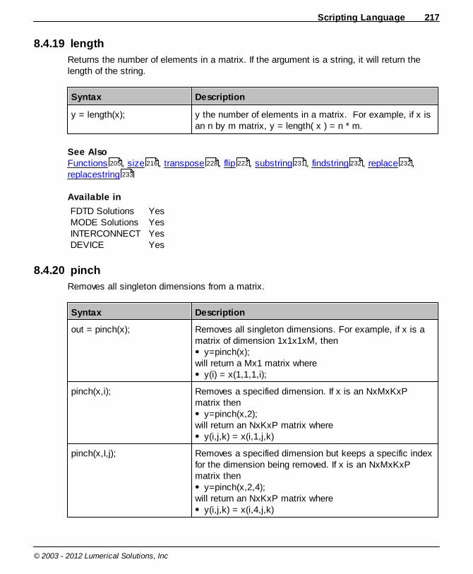
Scripting Language 217
© 2003 - 2012 Lumerical Solutions, Inc
8.4.19 length
Returns the number of elements in a matrix. If the argument is a string, it will return thelength of the string.
Syntax Description
y = length(x); y the number of elements in a matrix. For example, if x isan n by m matrix, y = length( x ) = n * m.
See AlsoFunctions , size , transpose , flip , substring , findstring , replace ,replacestring
Available in
FDTD SolutionsMODE SolutionsINTERCONNECTDEVICE
YesYesYesYes
8.4.20 pinch
Removes all singleton dimensions from a matrix.
Syntax Description
out = pinch(x); Removes all singleton dimensions. For example, if x is amatrix of dimension 1x1x1xM, then
y=pinch(x); will return a Mx1 matrix where
y(i) = x(1,1,1,i);
pinch(x,i); Removes a specified dimension. If x is an NxMxKxPmatrix then
y=pinch(x,2); will return an NxKxP matrix where
y(i,j,k) = x(i,1,j,k)
pinch(x,I,j); Removes a specified dimension but keeps a specific indexfor the dimension being removed. If x is an NxMxKxPmatrix then
y=pinch(x,2,4); will return an NxKxP matrix where
y(i,j,k) = x(i,4,j,k)
205 216 228 222 231 232 232
233

Reference Guide218
© 2003 - 2012 Lumerical Solutions, Inc
See AlsoFunctions , find , size , flip
Available in
FDTD SolutionsMODE SolutionsINTERCONNECTDEVICE
YesYesYesYes
8.4.21 sum
Sum of elements in a matrix.
Syntax Description
out = sum(x); Sum of all the elements in a matrix, over all dimensions.
out = sum(x,2); Sum x over the specified dimension.
See AlsoFunctions , integrate
Available in
FDTD SolutionsMODE SolutionsINTERCONNECTDEVICE
YesYesYesYes
8.4.22 max
The maximum value in a matrix. For complex numbers, only the real part is considered.
Syntax Description
out = max(x); The maximum value in a matrix.
See AlsoFunctions , min , abs
Available in
205 227 216 222
205 225
205 219 213
Scripting Language 219
© 2003 - 2012 Lumerical Solutions, Inc
FDTD SolutionsMODE SolutionsINTERCONNECTDEVICE
YesYesYesYes
8.4.23 min
The minimum value in a matrix. For complex numbers, only the real part is considered.
Syntax Description
out = min(x); The minimum value in a matrix.
See AlsoFunctions , max , abs
Available in
FDTD SolutionsMODE SolutionsINTERCONNECTDEVICE
YesYesYesYes
8.4.24 dot
Dot product.
Matrix A, B must have the same number of elements. The dot product will be calculatedwith the following formula.
i
iBiAC )()(
Syntax Description
C = dot(A, B); Returns the dot product of A and B
See Also Functions , cross , * , length , size
Available in
205 218 213
205 220 194 217 216
Reference Guide220
© 2003 - 2012 Lumerical Solutions, Inc
FDTD SolutionsMODE SolutionsINTERCONNECTDEVICE
YesYesYesYes
8.4.25 cross
Vector cross product.
Matrix A, B must be the same size. The cross product will be computed on the firstdimension that has a size of 3. There must be at least one dimension with a size of 3.
Assume that A,B are 2D matrices, where the second dimension contains the vectorcomponents. The size of the second dimension must be 3. Then the elements of C will becalculated with the standard cross product formulas.
)1,()2,()2,()1,()3,(
)1,()3,()3,()1,()2,(
)2,()3,()3,()2,()1,(
iBiAiBiAiC
iBiAiBiAiC
iBiAiBiAiC
Syntax Description
C = cross(A, B); Returns the cross product of A and B
See Also Functions , dot , * , length , size
Available in
FDTD SolutionsMODE SolutionsINTERCONNECTDEVICE
YesYesYesYes
8.4.26 eig
Find the eigen value and/or eigen vector of a matrix. The matrix has to be square.
Syntax Description
out = eig(A);out = eig(A, 1);
Returns the eigenvalues of matrix A.
205 219 194 217 216
Scripting Language 221
© 2003 - 2012 Lumerical Solutions, Inc
out = eig(A, 2); Returns the eigenvectors of matrix A.
out = eig(A, 3); Returns both the eigenvalues and eigenvectors of matrixA.
See AlsoOperators , = , == , != , <= , >= , < , > , & , and , | , or , !
, ~ , mult , permute , reshape , inv
Available in
FDTD SolutionsMODE SolutionsINTERCONNECTDEVICE
Yes, version 8+Yes, version 6+YesYes
8.4.27 mult
Perform matrix multiplication of two or more matrices. The dimensions of the matrices haveto match
Syntax Description
out = mult(A,B,...) Returns the matrix multiplication of matrices, A x B x C ...
See AlsoOperators , = , == , != , <= , >= , < , > , & , and , | , or , !
, ~ , eig , permute , reshape , inv
Available in
FDTD SolutionsMODE SolutionsINTERCONNECTDEVICE
Yes, version 8+Yes, version 6+YesYes
192 183 196 197 198 198 198 199 199 200 200 201
201 202 221 222 223 223
192 183 196 197 198 198 198 199 199 200 200 201
201 202 220 222 223 223
Reference Guide222
© 2003 - 2012 Lumerical Solutions, Inc
8.4.28 flip
Flip a matrix along one dimension.
Syntax Description
C = flip(A, dim); Flips the matrix A along the dimension dim.
See Also Functions , size , length , pinch , transpose
Available in
FDTD SolutionsMODE SolutionsINTERCONNECTDEVICE
YesYesYesYes
8.4.29 permute
This is an advanced version of the transpose function. It rearranges the dimensions of amatrix as specified by the second argument.
Syntax Description
out = permute(A, [i,j,k, ...]) Returns a matrix with the same elements as A but withrearranged dimensions i,j,k, etc.
See AlsoOperators , = , == , != , <= , >= , < , > , & , and , | , or , !
, ~ , eig , reshape , mult , inv
Available in
FDTD SolutionsMODE SolutionsINTERCONNECTDEVICE
Yes, version 8+Yes, version 6+YesYes
205 216 217 217 228
192 183 196 197 198 198 198 199 199 200 200 201
201 202 220 223 221 223

Scripting Language 223
© 2003 - 2012 Lumerical Solutions, Inc
8.4.30 reshape
Reshapes the matrix A to have the size i-by-j-by-k-by-... .The product of the specifieddimensions, i*j*k*..., must be the same as that of the original matrix A,
Syntax Description
out = reshape(A, [i,j,k, ...]) Returns an array with the same elements as A butreshaped to have the size i by j by k by ...
See AlsoOperators , = , == , != , <= , >= , < , > , & , and , | , or , !
, ~ , eig , permute , mult , inv
Available in
FDTD SolutionsMODE SolutionsINTERCONNECTDEVICE
Yes, version 8+Yes, version 6+YesYes
8.4.31 inv
Calculate the inverse of a matrix. The matrix has to be invertible.
Syntax Description
out = Inv(A) Returns the inverse of matrix A
See AlsoOperators , = , == , != , <= , >= , < , > , & , and , | , or , !
, ~ , eig , permute , mult , reshape
Available in
192 183 196 197 198 198 198 199 199 200 200 201
201 202 220 222 221 223
192 183 196 197 198 198 198 199 199 200 200 201
201 202 220 222 221 223

Reference Guide224
© 2003 - 2012 Lumerical Solutions, Inc
FDTD SolutionsMODE SolutionsINTERCONNECTDEVICE
Yes, version 8+Yes, version 6+YesYes
8.4.32 interp
Linear interpolation of a data set. The data can be complex.
Syntax Description
out = interp(Ex, xold,xnew);
Does a linear interpolation of a 1D function. Ex is existing dataxold specifies the points where Ex is sampledxnew specifies new point to interpolate the data.
The xnew does does not have to be within the bounds ofxold.
interp(Ex, xold, yold, xnew,ynew);
The 2D version of interp.
interp(Ex, xold, yold, zold,xnew, ynew, znew);
The 3D version of interp.
See Also Functions , spline
Available in
FDTD SolutionsMODE SolutionsINTERCONNECTDEVICE
YesYesYesYes
8.4.33 interptri
Triangular to linear interpolation of a data set. The data can be complex.
# Interpolate from triangular mesh to rectilinear meshEc_rect(1:nxspan,1:nyspan) = interptri(tri,vtx2,Ec(1:nvtx),xgrid,ygrid);
Syntax Description
205 225
Scripting Language 225
© 2003 - 2012 Lumerical Solutions, Inc
out = interptri(Elements,Vertices,Ex, xgrid, ygrid);
Does a triangular to linear interpolation of a function. Ex is existing dataxgrid/ygrid specifies the points where Ex is to besampled on the rectilinear meshElements are the elements of the triangular mesh takenfrom the simulation regionVertices are the vertices of the triangular mesh takenfrom the simulation region
8.4.34 spline
Does a cubic spline interpolation of a data set.
Syntax Description
out = spline(Ex,xold,xnew); Cubic spline interpolation of a 1D function. Ex is existing dataxold specifies the points where Ex is sampledxnew specifies new point to interpolate the data.
The xnew does does not have to be within the bounds ofxold.
See Also Functions , interp
Available in
FDTD SolutionsMODE SolutionsINTERCONNECTDEVICE
YesYesYesYes
8.4.35 integrate
Returns the integral over the specified dimension of a matrix.
Integrals over singleton dimensions will return zero (i.e. the area under a single point iszero). See integrate2 for an alternate behavior.
Syntax Description
out = integrate(A, n, x1); Integrates A over the nth dimension in the matrix.
205 224
Reference Guide226
© 2003 - 2012 Lumerical Solutions, Inc
x1 is the corresponding position vector for that dimension.
out = integrate(A, d, x1,x2, ...);
Calculates the integral of A over the specified list ofdimension(s) d.d is a vector containing the dimensions over which tointegrate.xi are the position vectors corresponding to the dimensionsof A over which the integration is occurring. For example
power = integrate(A,1:2,x,y) will integrate A over an x-ysurface.
See Also Functions , integrate2 , max , min , interp , find , pinch , round ,getdata , sum , length
Available in
FDTD SolutionsMODE SolutionsINTERCONNECTDEVICE
YesYesYesYes
8.4.36 integrate2
Very similar to the standard integrate function, except that singleton dimensions aretreated differently.
As described in the integrate function description, integrating over dimensions with a singlevalue (singleton dimensions) returns zero because the area under a single point is zero. Insome cases, particularly when you are not sure which dimensions are singleton, thisbehavior can cause difficulties. The integrate2 function automatically ignores alldimensions with a size of one, which avoids the problem of a zero valued integrals due tosingleton dimensions.
Syntax Description
out = integrate2(A, 1, x1); Integrates A over the first dimension in the matrix. x1 is the corresponding position vector.
out = integrate2(A, d, x1, x2,...);
Calculates the integral of A over the specified dimension(s)d.d is a vector containing the dimensions over which tointegrate.
205 226 218 219 224 227 217 247
349 218 217
Scripting Language 227
© 2003 - 2012 Lumerical Solutions, Inc
xi is the position vector corresponding to the dimensions ofA over which the integration is occurring. If any of the xivectors only have 1 element, integrate returns 0.For example
power = integrate2(A,1:2,x,y) will integrate A over an x-ysurface.
See Also Functions , integrate , max , min , interp , find , pinch , round ,getdata , sum , length
Available in
FDTD SolutionsMODE SolutionsINTERCONNECTDEVICE
Version 8+Version 6+YesYes
8.4.37 find
This function will search for entries in a matrix that meet some condition. The indices ofthose values are returned.For multi-dimensional matrixes, the find function will still return a single index. This isuseful when using the output from find in a loop.
Syntax Description
out = find(x,5e-6); Will return the index of x that corresponds to the closestvalue to 5e-6.
out = find(x>5); Will return indices of all values of x that are greater than 5.
See AlsoFunctions , pinch , findpeaks , integrate , length
Available in
FDTD SolutionsMODE SolutionsINTERCONNECTDEVICE
YesYesYesYes
205 225 218 219 224 227 217 247
349 218 217
205 217 228 225 217
Reference Guide228
© 2003 - 2012 Lumerical Solutions, Inc
8.4.38 findpeaks
Returns the position of peaks in a matrix. A peak is defined as a data point that is largerthan its nearest neighbors.
Syntax Description
out = findpeaks(y); Returns the position of the peak with the largest value in y.The length of y must be at least 2. If no peak is found inthe data, a value of 1 is returned.
findpeaks(y,n); Returns a matrix containing the positions of the largest npeaks found in the data. The returned values are orderedfrom largest to smallest. The returned matrix is always ofdimension nX1. If less than n peaks are found, theremaining values of the returned matrix are 1.
See AlsoFunctions , find
Available in
FDTD SolutionsMODE SolutionsINTERCONNECTDEVICE
YesYesYesYes
8.4.39 transpose
Transpose a 1D or 2D matrix.
Syntax Description
y = transpose(x); If x is an N x M matrix, then y will be M x N, where theentries are y(j,i)=x(i,j).
See AlsoFunctions , ctranspose , flip
Available in
FDTD SolutionsMODE SolutionsINTERCONNECTDEVICE
YesYesYesYes
205 227
205 229 222
Scripting Language 229
© 2003 - 2012 Lumerical Solutions, Inc
8.4.40 ctranspose
Transpose a 1D or 2D matrix and take the complex conjugate of each element.
Syntax Description
y = ctranspose(x); If x is an N x M matrix, then y will be M x N, where the
entries are y(j,i)=x(i,j)*.
See AlsoFunctions , transpose
Available in
FDTD SolutionsMODE SolutionsINTERCONNECTDEVICE
YesYesYesYes
8.4.41 num2str
Convert an integer, floating point number, or matrix into a string. Use the format scriptcommand to change the precision of the output.
Syntax Description
out = num2str(x); Converts the number x into a string. x can also be a 1D or2D matrix.
See AlsoOperators , " , + , ? , endl , write , format ,str2num , findstring ,replace , replacestring , substring
Available in
FDTD SolutionsMODE SolutionsINTERCONNECTDEVICE
YesYesYesYes
205 228
192 202 195 204 204 175 173 230 232
232 233 231
Reference Guide230
© 2003 - 2012 Lumerical Solutions, Inc
8.4.42 str2num
Convert a string into a floating point number. Use the format script command to change theprecision of the output.
Syntax Description
out = str2num(string); Converts string into a number.
See AlsoOperators , " , + , ? , endl , write , format , findstring , replace ,replacestring , substring
Available in
FDTD SolutionsMODE SolutionsINTERCONNECTDEVICE
YesYesYesYes
8.4.43 eval
Execute string containing Lumerical scripting language.
Syntax Description
eval(string); Execute string containing Lumerical scripting language atthe Lumerical script prompt.This function does not return any data.
See AlsoOperators , feval , str2num , num2str
Available in
FDTD SolutionsMODE SolutionsINTERCONNECTDEVICE
YesYesYesYes
192 202 195 204 204 175 173 232 232
233 231
192 231 230 229

Scripting Language 231
© 2003 - 2012 Lumerical Solutions, Inc
8.4.44 feval
Evaluates a string as script file. This function is useful for running script files that are not inyour path and files with spaces in the name.
Syntax Description
feval(filename); Execute string containing the name of a script file at theLumerical script prompt.This function does not return any data.
See AlsoOperators , eval , str2num , num2str
Available in
FDTD SolutionsMODE SolutionsINTERCONNECTDEVICE
YesYesYesYes
8.4.45 substring
Can be used to extract a substring from a string.
Syntax Description
s1 = substring(s,pos); Returns a substring of s, starting at position pos to the endof s. The position pos can be 1 to length(s).
s1 = substring(s,pos,len); Returns a substring of s, starting at position pos, with lencharacters. If len is -1 (or any value less than 0) it returnsthe substring at position pos to the end of s. The defaultvalue of len is -1.
See AlsoFunctions , length , findstring , replace , replacestring , str2num , num2str
Available in
FDTD SolutionsMODE SolutionsINTERCONNECTDEVICE
YesYesYesYes
192 230 230 229
205 217 232 232 233 230
229
Reference Guide232
© 2003 - 2012 Lumerical Solutions, Inc
8.4.46 findstring
Returns the position of a given substring in a string.
Syntax Description
pos = findstring(s,s1); Returns the position of the first instance substring s1 in s.If s1 is not found in s, it returns -1.
pos = findstring(s,s1,p0); Returns the position of the first instance substring s1 in s,starting at position p0. If s1 is not found in s, starting fromp0, it returns -1.
See AlsoFunctions , length , substring , replace , replacestring , str2num , num2str
Available in
FDTD SolutionsMODE SolutionsINTERCONNECTDEVICE
YesYesYesYes
8.4.47 replace
Replaces a substring of a string with a new string.
Syntax Description
snew = replace(s,pos,len,s1);
Replaces len characters of s, starting at position pos, withthe string in s1. If len is 0, it will insert the string s1between pos-1 and pos. If len is -1 (or any values less than0) it will replace all remaining characters in s with s1,starting at pos. The position pos can be 1 to length(s).
See AlsoFunctions , length , substring , findstring , replacestring , str2num ,num2str
Available in
205 217 231 232 233 230
229
205 217 231 232 233 230
229
Scripting Language 233
© 2003 - 2012 Lumerical Solutions, Inc
FDTD SolutionsMODE SolutionsINTERCONNECTDEVICE
YesYesYesYes
8.4.48 replacestring
Replaces a substring of a string with a new string.
Syntax Description
snew = replacestring(s,s1,s2);
Replaces all instances of s1 in s with s2.
See AlsoFunctions , length , substring , findstring , replace , str2num , num2str
Available in
FDTD SolutionsMODE SolutionsINTERCONNECTDEVICE
YesYesYesYes
8.4.49 fft
Compute the 1D, 2D or 3D Fast Fourier Transform (fft) of a matrix. In the 1D case thetransform is given by
)1)(1)(2
(
1
][)(][mn
N
iN
nxxw enEEfftmE
The fft, inverse fft and all associated functions have an option (option 1 below) that controlsthe format used to store the frequency domain data. When working with spectral data it isnot possible to switch between formats; there are no functions to convert between formats.This implies that if you use option 1=n to produce a spectrum with fft, then you must alsouse option 1=n if you want to pass that same spectral data to invfft. Similarly, if you useoption 1=n for fft, then you also need to use option 1=n with fftw to get the proper frequencyvector corresponding to your spectrum. invfft and fftk work in the same way.
Syntax Description
out = fft(Ex); Returns the fast Fourier transform of Ex. Ex can be 1D, 2D
205 217 231 232 232 230 229
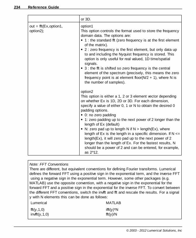
Reference Guide234
© 2003 - 2012 Lumerical Solutions, Inc
or 3D.
out = fft(Ex,option1,option2);
option1 This option controls the format used to store the frequencydomain data. The options are:
1 : the standard fft (zero frequency is at the first elementof the matrix). 2 : zero frequency is the first element, but only data upto and including the Nyquist frequency is stored. Thisoption is only useful for real valued, 1D time/spatialsignals.3 : the fft is shifted so zero frequency is the centralelement of the spectrum (precisely, this means the zerofrequency point is at element floor(N/2 + 1), where N isthe number of samples).
option2 This option is either a 1, 2 or 3 element vector dependingon whether Ex is 1D, 2D or 3D. For each dimension,specify a value of either 0, 1 or N to obtain the desired 0padding options.
0: no zero padding1: zero padding up to the next power of 2 longer than thelength of Ex (default)N: zero pad up to length N if N > length(Ex), wherelength of Ex is the length in a specific dimension. If N <=length(Ex), it will zero pad up to the next power of 2longer than the length of Ex. For the fastest results, Nshould be a power of 2 and can be entered, for example,as 2 12.
Note: FFT ConventionsThere are different, but equivalent conventions for defining Fourier transforms. Lumericaldefines the forward FFT using a positive sign in the exponential term, and the inverse FFT using a negative sign in the exponential term. However, some other packages (e.g.MATLAB) use the opposite convention, with a negative sign in the exponential for theforward FFT and a positive sign in the exponential for the inverse FFT. To convert betweenthe different FFT conventions, switch the invfft and fft and rescale the results. For a signaly with N elements this can be done as follows:
Lumerical MATLAB
fft(y,1,0)invfft(y,1,0)
ifft(y)*N fft(y)/N
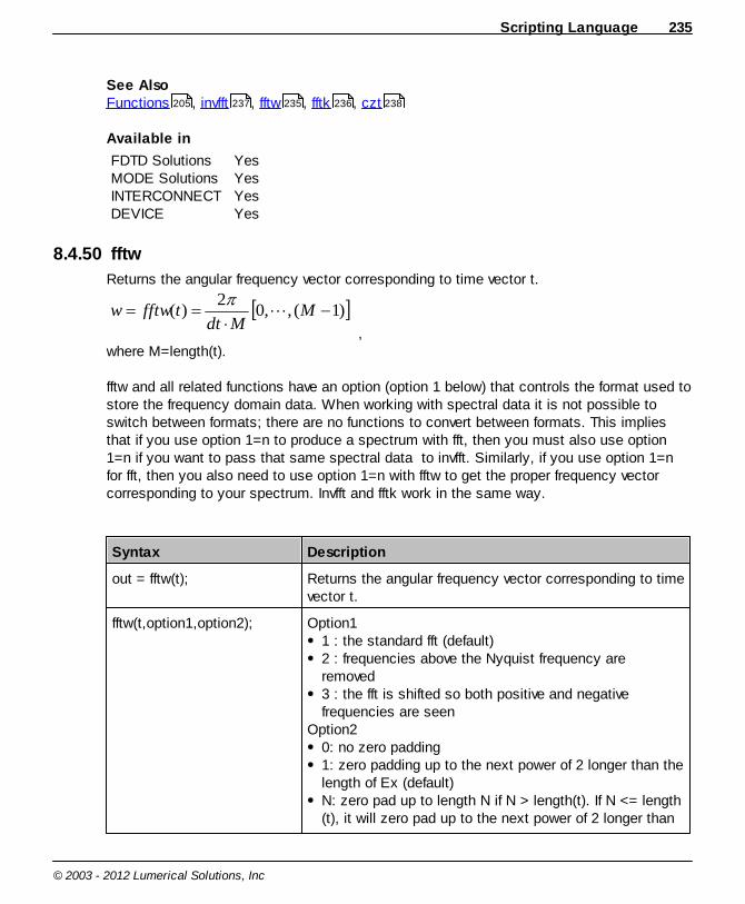
Scripting Language 235
© 2003 - 2012 Lumerical Solutions, Inc
See Also Functions , invfft , fftw , fftk , czt
Available in
FDTD SolutionsMODE SolutionsINTERCONNECTDEVICE
YesYesYesYes
8.4.50 fftw
Returns the angular frequency vector corresponding to time vector t.
)1(,,02
)( MMdt
tfftww
,where M=length(t).
fftw and all related functions have an option (option 1 below) that controls the format used tostore the frequency domain data. When working with spectral data it is not possible toswitch between formats; there are no functions to convert between formats. This impliesthat if you use option 1=n to produce a spectrum with fft, then you must also use option1=n if you want to pass that same spectral data to invfft. Similarly, if you use option 1=nfor fft, then you also need to use option 1=n with fftw to get the proper frequency vectorcorresponding to your spectrum. Invfft and fftk work in the same way.
Syntax Description
out = fftw(t); Returns the angular frequency vector corresponding to timevector t.
fftw(t,option1,option2); Option1 1 : the standard fft (default) 2 : frequencies above the Nyquist frequency areremoved 3 : the fft is shifted so both positive and negativefrequencies are seen
Option20: no zero padding1: zero padding up to the next power of 2 longer than thelength of Ex (default)N: zero pad up to length N if N > length(t). If N <= length(t), it will zero pad up to the next power of 2 longer than
205 237 235 236 238

Reference Guide236
© 2003 - 2012 Lumerical Solutions, Inc
the length of t. For the fastest results, N should be apower of 2 and can be entered, for example, as 2 12.
See Also Functions , fft , fftk , invfft
Available in
FDTD SolutionsMODE SolutionsINTERCONNECTDEVICE
YesYesYesYes
8.4.51 fftk
Returns the spatial wavevector kx associated with a fourier transform of a function of x.
)1(,,02
)( MMdx
xfftkk
,where M=length(x).
fftk and all related functions have an option (option 1 below) that controls the format used tostore the frequency domain data. When working with spectral data it is not possible toswitch between formats; there are no functions to convert between formats. This impliesthat if you use option 1=n to produce a spectrum with fft, then you must also use option1=n if you want to pass that same spectral data to invfft. Similarly, if you use option 1=nfor fft, then you also need to use option 1=n with fftw to get the proper frequency vectorcorresponding to your spectrum. Invfft and fftk work in the same way.
Syntax Description
out = fftk(x); Returns the spatial wavevector kx associated with a fouriertransform of a function of x..
fftk(x,option1,option2); Option1 1 : the standard fft (default) 2 : frequencies above the Nyquist frequency areremoved 3 : the fft is shifted so both positive and negativefrequencies are seen
Option20: no zero padding 1: zero padding up to the next power of 2 longer than thelength of Ex (default)
205 233 236 237
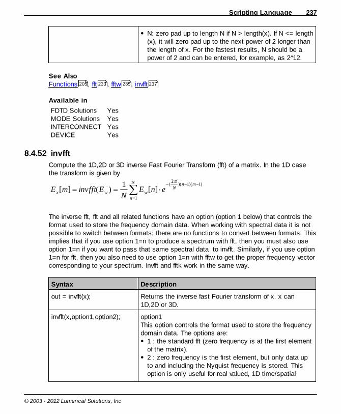
Scripting Language 237
© 2003 - 2012 Lumerical Solutions, Inc
N: zero pad up to length N if N > length(x). If N <= length(x), it will zero pad up to the next power of 2 longer thanthe length of x. For the fastest results, N should be apower of 2 and can be entered, for example, as 2 12.
See Also Functions , fft , fftw , invfft
Available in
FDTD SolutionsMODE SolutionsINTERCONNECTDEVICE
YesYesYesYes
8.4.52 invfft
Compute the 1D,2D or 3D inverse Fast Fourier Transform (fft) of a matrix. In the 1D casethe transform is given by
)1)(1)(2
(
1
][1
)(][mn
N
iN
nwwx enE
NEinvfftmE
The inverse fft, fft and all related functions have an option (option 1 below) that controls theformat used to store the frequency domain data. When working with spectral data it is notpossible to switch between formats; there are no functions to convert between formats. Thisimplies that if you use option 1=n to produce a spectrum with fft, then you must also useoption 1=n if you want to pass that same spectral data to invfft. Similarly, if you use option1=n for fft, then you also need to use option 1=n with fftw to get the proper frequency vectorcorresponding to your spectrum. Invfft and fftk work in the same way.
Syntax Description
out = invfft(x); Returns the inverse fast Fourier transform of x. x can1D,2D or 3D.
invfft(x,option1,option2); option1 This option controls the format used to store the frequencydomain data. The options are:
1 : the standard fft (zero frequency is at the first elementof the matrix). 2 : zero frequency is the first element, but only data upto and including the Nyquist frequency is stored. Thisoption is only useful for real valued, 1D time/spatial
205 233 235 237
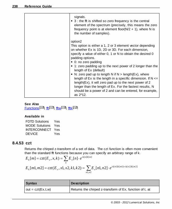
Reference Guide238
© 2003 - 2012 Lumerical Solutions, Inc
signals.3 : the fft is shifted so zero frequency is the centralelement of the spectrum (precisely, this means the zerofrequency point is at element floor(N/2 + 1), where N isthe number of samples).
option2 This option is either a 1, 2 or 3 element vector dependingon whether Ex is 1D, 2D or 3D. For each dimension,specify a value of either 0, 1 or N to obtain the desired 0padding options.
0: no zero padding1: zero padding up to the next power of 2 longer than thelength of Ex (default)N: zero pad up to length N if N > length(Ex), wherelength of Ex is the length in a specific dimension. If N <=length(Ex), it will zero pad up to the next power of 2longer than the length of Ex. For the fastest results, Nshould be a power of 2 and can be entered, for example,as 2 12.
See Also Functions , fft , fftw , fftk
Available in
FDTD SolutionsMODE SolutionsINTERCONNECTDEVICE
YesYesYesYes
8.4.53 czt
Returns the chirped z-transform of a set of data. The czt function is often more convenientthan the standard fft functions because you can specify an arbitrary range of k.
2,1
]2[]2[]1[]1[
][][
]2,1[)2,1,2,1,(]2,1[
][),,(][
nn
mknixmknixxxk
n
mknixxxk
ennEkkxxEcztmmE
enEkxEcztmE
Syntax Description
out = czt(Ex,t,w) Returns the chirped z-transform of Ex, function of t, at
205 233 235 236
Scripting Language 239
© 2003 - 2012 Lumerical Solutions, Inc
each desired angular frequency w. Note that w must be alinearly spaced set of angular frequencies but can coverany range.
czt(Ex,x,y,kx,ky); The two dimensional chirped z-transform. kx and ky mustbe linearly spaced sets of wavenumbers but can cover anyrange.
See Also Functions , fft
Available in
FDTD SolutionsMODE SolutionsINTERCONNECTDEVICE
YesYesYesYes
8.4.54 polyarea
Returns the area of a polygon. The area is positive if the vertices are defined in a counter-clockwise direction, and negative if the vertices are defined in a clockwise direction.
The polygon vertices are contained in a single matrix of dimension Nx2 (or 2xN) where N>= 3. The second dimension represents the x,y positions. For example, a valid polygon isV = [ 0,0; 1,0; 1,1; 0,1];
Syntax Description
out = polyarea(V); Returns the area of V. The sign of the area indicates if V isdefined in a counter-clockwise (positive) or clockwise(negative) direction.
See Also Functions , centroid , polyintersect , inpoly , polygrow , polyand , polyor
, polydiff , polyxor
Available in
FDTD SolutionsMODE SolutionsINTERCONNECTDEVICE
YesYesYesYes
205 233
205 240 240 241 241 242
242 243 244
Reference Guide240
© 2003 - 2012 Lumerical Solutions, Inc
8.4.55 centroid
Returns the center of mass of a polygon.
The polygon vertices are contained in a single matrix of dimension Nx2 (or 2xN) where N>= 3. The second dimension represents the x,y positions. For example, a valid polygon isV = [ 0,0; 1,0; 1,1; 0,1];
Syntax Description
out = centroid(V); Returns the center of mass of V, assuming uniformdensity. The output is a 2x1 matrix representing the x andy positions.
See Also Functions , polyarea , polyintersect , inpoly , polygrow , polyand , polyor
, polydiff , polyxor
Available in
FDTD SolutionsMODE SolutionsINTERCONNECTDEVICE
YesYesYesYes
8.4.56 polyintersect
Determines if two polygons intersect. This command is available in FDTD Solutions 7.0. Itis not available in MODE Solutions 4.0.
The polygon vertices are contained in a single matrix of dimension Nx2 (or 2xN) where N>= 3. The second dimension represents the x,y positions. For example, a valid polygon isV = [ 0,0; 1,0; 1,1; 0,1];
Syntax Description
out = polyintersect(V1,V2); Returns0 if the polygons do not overlap0.5 if the polygons touch1 if they overlap2 if one polygon completely encloses the other
See Also
205 239 240 241 241 242
242 243 244
Scripting Language 241
© 2003 - 2012 Lumerical Solutions, Inc
Functions , polyarea , centroid , inpoly , polygrow , polyand , polyor ,polydiff , polyxor
Available in
FDTD SolutionsMODE SolutionsINTERCONNECTDEVICE
YesYesYesYes
8.4.57 inpoly
Determines if a point is inside our outside a polygon. The function is vectorized so it can beused to create a mesh of a polygon.
The polygon vertices are contained in a single matrix of dimension Nx2 (or 2xN) where N>= 3. The second dimension represents the x,y positions. For example, a valid polygon isV = [ 0,0; 1,0; 1,1; 0,1];
Syntax Description
out = inpoly(V,x,y); Returns a matrix of the same dimension of x with 1 if thecorresponding point is inside the polygon and 0 otherwise.The matrices x and y must have the same length, or one ofthem can be a singleton.
See Also Functions , polyarea , centroid , polyintersect , polygrow , polyand , polyor
, polydiff , polyxor
Available in
FDTD SolutionsMODE SolutionsINTERCONNECTDEVICE
YesYesYesYes
8.4.58 polygrow
Returns a polygon that has grown or shrunk by the specified amount. The polygon is grownin a direction normal to every line segment.
The polygon vertices are contained in a single matrix of dimension Nx2 (or 2xN) where N>= 3. The second dimension represents the x,y positions. For example, a valid polygon isV = [ 0,0; 1,0; 1,1; 0,1];
205 239 240 241 241 242 242
243 244
205 239 240 240 241 242
242 243 244

Reference Guide242
© 2003 - 2012 Lumerical Solutions, Inc
Syntax Description
out = plygrow(V,dx); Returns a new polygon that has grown by dx. To shrink apolygon, use dx < 0.
See Also Functions , polyarea , centroid , polyintersect , inpoly , polyand , polyor
, polydiff , polyxor
Available in
FDTD SolutionsMODE SolutionsINTERCONNECTDEVICE
YesYesYesYes
8.4.59 polyand
Combines two polygons into one using a boolean and operation.
The polygon vertices are contained in a single matrix of dimension Nx2 (or 2xN) where N>= 3. The second dimension represents the x,y positions. For example, a valid polygon isV = [ 0,0; 1,0; 1,1; 0,1];
Syntax Description
V3 = polyand(V1,V2); Returns a new polygon, V3, that is the and of V1 and V2.
See Also Functions , polyor , polydiff , polyxor , polyarea , centroid , polyintersect
, inpoly , polygrow
Available in
FDTD SolutionsMODE SolutionsINTERCONNECTDEVICE
YesYesYesYes
8.4.60 polyor
Combines two polygons into one using a boolean or operation.
The polygon vertices are contained in a single matrix of dimension Nx2 (or 2xN) where N>= 3. The second dimension represents the x,y positions. For example, a valid polygon is
205 239 240 240 241 242
242 243 244
205 242 243 244 239 240
240 241 241
Scripting Language 243
© 2003 - 2012 Lumerical Solutions, Inc
V = [ 0,0; 1,0; 1,1; 0,1];
Syntax Description
V3 = polyor(V1,V2); Returns a new polygon, V3, that is the or of V1 and V2.
See Also Functions , polyand , polydiff , polyxor , polyarea , centroid , polyintersect
, inpoly , polygrow
Available in
FDTD SolutionsMODE SolutionsINTERCONNECTDEVICE
YesYesYesYes
8.4.61 polydiff
Combines two polygons into one by taking the difference.
The polygon vertices are contained in a single matrix of dimension Nx2 (or 2xN) where N>= 3. The second dimension represents the x,y positions. For example, a valid polygon isV = [ 0,0; 1,0; 1,1; 0,1];
Syntax Description
V3 = polydiff(V1,V2); Returns a new polygon, V3, that is V1-V2.
See Also Functions , polyand , polyor , polyxor , polyarea , centroid , polyintersect
, inpoly , polygrow
Available in
FDTD SolutionsMODE SolutionsINTERCONNECTDEVICE
YesYesYesYes
205 242 243 244 239 240
240 241 241
205 242 242 244 239 240
240 241 241
Reference Guide244
© 2003 - 2012 Lumerical Solutions, Inc
8.4.62 polyxor
Combines two polygons into one using a boolean xor operation.
The polygon vertices are contained in a single matrix of dimension Nx2 (or 2xN) where N>= 3. The second dimension represents the x,y positions. For example, a valid polygon isV = [ 0,0; 1,0; 1,1; 0,1];
Syntax Description
V3 = polyxor(V1,V2); Returns a new polygon, V3, that is the xor of V1 and V2.
See Also Functions , polyand , polyor , polydiff , polyarea , centroid , polyintersect
, inpoly , polygrow
Available in
FDTD SolutionsMODE SolutionsINTERCONNECTDEVICE
YesYesYesYes
8.4.63 lineintersect
Returns the intersection points of lines in the x-y plane. Note that the intersection pointdoes not have to lie on the line segments themselves that define the lines. To see if the linesegments actually cross the command linecross should be used.
Line segments are contained in a single matrix of dimension 2*Nx2, where there are N linesegments. For example, the matrix L = [ 0,0; 1,1; 0,0, 0,1]; represents 2 lines segments,one from (0,0) to (1,1) and another from (0,0) to (0,1).
Syntax Description
out = lineintersect(L1,L2); Returns the intersection of the lines represented by thesegments in L1 and L2. L1 and L2 must have the samesize (2*N,2 for N line segments). The result is a sequenceof x,y points in the form Nx2 representing the intersectionsof the N lines. There are special cases when
The lines are parallel. In this case, the position returnedis (1.#INF,b). The value of 1.#INF can be tested for usingthe script commands finite. The value of b is 0 if the linesare not coincident and 1 if they are coincident.The points in a segment are degenerate, ie the same. In
205 242 242 243 239 240
240 241 241
Scripting Language 245
© 2003 - 2012 Lumerical Solutions, Inc
this case, the position returned is (1.#INF,b), where b is0, 1, 2 if the both line segments are degenerate, the firstis degenerate, or the second is degenerate respectively.
See Also Functions , linecross , finite
Available in
FDTD SolutionsMODE SolutionsINTERCONNECTDEVICE
YesYesYesYes
8.4.64 linecross
Determines if line segments cross each other.
Line segments are contained in a single matrix of dimension 2*Nx2, where there are N linesegments. For example, the matrix L = [ 0,0; 1,1; 0,0, 0,1]; represents 2 lines segments,one from (0,0) to (1,1) and another from (0,0) to (0,1).
Syntax Description
out = linecross(L1,L2); Returns a matrix of dimension N which determines if the Nline segments in L1 and the N line segments in L2 cross.L1 and L2 must have the same size (2*Nx2 for N linesegments). The result is a matrix of length N that is 0 ifthe segments do not cross, 1 if they cross and 0.5 if theendpoint of one line touches another. Line segments thatare coincident and touch also return a value of 0.5
See Also Functions , lineintersect , finite
Available in
FDTD SolutionsMODE SolutionsINTERCONNECTDEVICE
YesYesYesYes
205 245 249
205 244 249
Reference Guide246
© 2003 - 2012 Lumerical Solutions, Inc
8.4.65 ceil
The ceil command rounds the input to the nearest integer greater than or equal to itself.
Syntax Description
out = ceil(X); Returns the nearest integer greater than or equal to X.
See AlsoFunctions , floor , mod
Available in
FDTD SolutionsMODE SolutionsINTERCONNECTDEVICE
YesYesYesYes
8.4.66 floor
The floor command rounds the input to the nearest integer less than or equal to itself.
Syntax Description
out = floor(X); Returns the nearest integer less than or equal to X.
See AlsoFunctions , ceil , mod
Available in
FDTD SolutionsMODE SolutionsINTERCONNECTDEVICE
YesYesYesYes
8.4.67 mod
Modulus after division.
Syntax Description
out = mod(X,Y); Returns X - n.*Y where n = floor(X./Y) if Y is not equal to 0.The input X must be a real array or a real scalar. Y mustbe a real scalar.
205 246 246
205 246 246
Scripting Language 247
© 2003 - 2012 Lumerical Solutions, Inc
The following are true by convention:mod(X,0) = Xmod(X,X) = 0
See AlsoFunctions , floor , ceil
Available in
FDTD SolutionsMODE SolutionsINTERCONNECTDEVICE
YesYesYesYes
8.4.68 sign
Get the sign of a number.
Syntax Description
out = sign(data); Real valuessign = 0 for data=0sign = 1 for data>0sign =-1 for data<0
Complex valuessign = 0 for data=0+0isign = data/abs(data) for data!=0
See AlsoFunctions , floor , ceil
Available in
FDTD SolutionsMODE SolutionsINTERCONNECTDEVICE
Version 8+Version 6+Version 2+Yes
8.4.69 round
Rounds a number to the nearest integer.
Syntax Description
205 246 246
205 246 246

Reference Guide248
© 2003 - 2012 Lumerical Solutions, Inc
out = round(x); Rounds x to the nearest integer.
See AlsoFunctions
Available in
FDTD SolutionsMODE SolutionsINTERCONNECTDEVICE
YesYesYesYes
8.4.70 rand
Generate a uniform random number between 0 and 1.
Syntax Description
out = rand; Generates a uniform random number between 0 and 1.
out = rand(min,max); Generates a random number between min and max. Bydefault, min and max are 0 and 1 respectively.
out = rand(min,max,option); option = 1: output is a double precision number betweenmin and max (default)option = 2: output is an integer between min and max.
See AlsoFunctions , randreset , randmatrix
Available in
FDTD SolutionsMODE SolutionsINTERCONNECTDEVICE
YesYesYesYes
8.4.71 randreset
Resets the random number generator seed.
Syntax Description
out = randreset; Resets the random number seed based on the clock time.This function returns the random number seed that was
205
205 248 186

Scripting Language 249
© 2003 - 2012 Lumerical Solutions, Inc
used.
out = randreset(seed); Set the seed to a specific value
See AlsoFunctions , rand , randmatrix
Available in
FDTD SolutionsMODE SolutionsINTERCONNECTDEVICE
YesYesYesYes
8.4.72 finite
The finite command returns 1 (true) if a value is finite. Numbers such as NaN or #1.INFreturn 0 (false).
Syntax Description
out = finite(x); Returns a matrix of the same size as x. The values are 1for values of x that are finite and 0 for values that are NaN.For example, finite(1/0) returns 0.
See AlsoFunctions
Available in
FDTD SolutionsMODE SolutionsINTERCONNECTDEVICE
YesYesYesYes
8.4.73 solar
Returns the solar power spectrum, in Watts/meter 2/meter.
Syntax Description
out = solar(1); Returns the power of the solar spectrum as a function ofwavelength, in W/m 2/m
out = solar(0); Returns the corresponding wavelength vector, in m
205 248 186
205

Reference Guide250
© 2003 - 2012 Lumerical Solutions, Inc
Available in
FDTD SolutionsMODE SolutionsINTERCONNECTDEVICE
NoNoNoYes
See Also plot , integrate
8.4.74 stackrt
Calculates reflection and transmission of a plane wave through a multi-layer stack.
Syntax Description
RT = stackrt(n,d,f); RT is a data set that contains the fraction of reflected andtransmitted power, and complex r,t coefficients for both Sand P polarizations.
Arguments for a stack with Nlayer:n: Refractive index of each layer. Size is either Nlayers, orNlayers x length(f) if dispersive materials are involvedd: Thickness of each layer. Size is Nlayers. The thicknessof the first and last layers is not important, as they areassumed to be infinite.f: Frequency vector.
RT = stackrt(n,d,f,theta); theta: Angle vector, in degrees. Optional.
Available in
FDTD SolutionsMODE SolutionsINTERCONNECTDEVICE
FDTD 8NoNoNo
See Also Functions
253 225
205
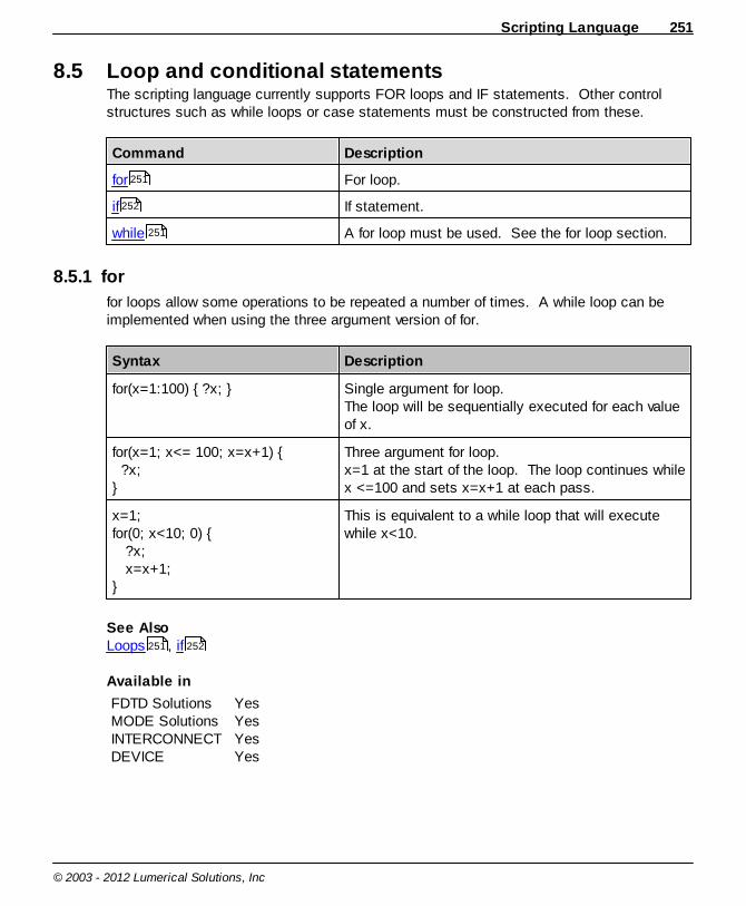
Scripting Language 251
© 2003 - 2012 Lumerical Solutions, Inc
8.5 Loop and conditional statementsThe scripting language currently supports FOR loops and IF statements. Other controlstructures such as while loops or case statements must be constructed from these.
Command Description
for For loop.
if If statement.
while A for loop must be used. See the for loop section.
8.5.1 for
for loops allow some operations to be repeated a number of times. A while loop can beimplemented when using the three argument version of for.
Syntax Description
for(x=1:100) { ?x; } Single argument for loop.The loop will be sequentially executed for each valueof x.
for(x=1; x<= 100; x=x+1) { ?x; }
Three argument for loop. x=1 at the start of the loop. The loop continues whilex <=100 and sets x=x+1 at each pass.
x=1;for(0; x<10; 0) { ?x; x=x+1;}
This is equivalent to a while loop that will executewhile x<10.
See Also Loops , if
Available in
FDTD SolutionsMODE SolutionsINTERCONNECTDEVICE
YesYesYesYes
251
252
251
251 252

Reference Guide252
© 2003 - 2012 Lumerical Solutions, Inc
8.5.2 if
The scripting language supports if statements in the following forms:
Syntax Description
if(x < 5) { y = x 2; } Simple if statement on one line.
if(x < 5) { y = x 2; }
Multi-line if statement
if(x < 5) { y = x 2; } else { y = x 3; }
If else statement.
if(x < 5) { if(x > 0) {y = x 2; } } else { y = x 3; }
Nested if statement with else.
See Also Loops , for
Available in
FDTD SolutionsMODE SolutionsINTERCONNECTDEVICE
YesYesYesYes
8.6 Plotting commandsLine and image plots are supported. These figures can be exported to jpeg images.
Plotting functions.
Command Description
plot Makes line plots.
plotxy Makes line plots, when data sets are sampled atdifferent position vectors.
polar Makes polar plots.
251 251
253
254
255

Scripting Language 253
© 2003 - 2012 Lumerical Solutions, Inc
polar2 Makes polar plots, when data sets are sampled atdifferent position vectors.
polarimage Makes a 2D polar image plot.
legend Makes a legend on a figure with line plots.
image Makes 2D image plots.
setplot Sets figure properties.
visualize Pass in simulation data to the visualizer.
Miscellaneous plotting functions.
Command Description
selectfigure Selects a figure.
exportfigure Exports a figure.
closeall Closes all figure windows.
8.6.1 plot
Create line plots. All data sets must be sampled on the same position vector.
See plotxy for data sets that are sampled on different position vectors.
Syntax Description
out = plot(x,y); Creates a plot of y vs x, y and x are both 1D vectors withthe same length. The figure number is returned.
plot(x,y); x is a nx1 matrix.y is a nxm matrix.This will generate a graph with m lines. (y(1:n,1) vs x, y(1:n,2) vs x, etc)
plot(x,y1,y2,y3); Creates a plot with 3 curves, x,y1, y2, y3 must be thesame length, returns the figure number.
plot(x,y, "x label", "y label","title");
Creates a plot of y vs x with axis labels and a title, returnsthe figure number.
plot(x,y, "x label", "y label","title", "options");
Creates a plot with desired options. Options can be be logplot plot lines OR plot points
256
257
257
258
260
259
259
260
261
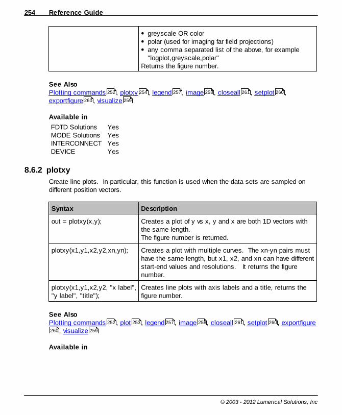
Reference Guide254
© 2003 - 2012 Lumerical Solutions, Inc
greyscale OR colorpolar (used for imaging far field projections)any comma separated list of the above, for example"logplot,greyscale,polar"
Returns the figure number.
See Also Plotting commands , plotxy , legend , image , closeall , setplot ,exportfigure , visualize
Available in
FDTD SolutionsMODE SolutionsINTERCONNECTDEVICE
YesYesYesYes
8.6.2 plotxy
Create line plots. In particular, this function is used when the data sets are sampled ondifferent position vectors.
Syntax Description
out = plotxy(x,y); Creates a plot of y vs x, y and x are both 1D vectors withthe same length. The figure number is returned.
plotxy(x1,y1,x2,y2,xn,yn); Creates a plot with multiple curves. The xn-yn pairs musthave the same length, but x1, x2, and xn can have differentstart-end values and resolutions. It returns the figurenumber.
plotxy(x1,y1,x2,y2, "x label","y label", "title");
Creates line plots with axis labels and a title, returns thefigure number.
See Also Plotting commands , plot , legend , image , closeall , setplot , exportfigure
, visualize
Available in
252 254 257 258 261 260
260 259
252 253 257 258 261 260
260 259

Scripting Language 255
© 2003 - 2012 Lumerical Solutions, Inc
FDTD SolutionsMODE SolutionsINTERCONNECTDEVICE
YesYesYesYes
8.6.3 polar
Create polar plots. All data sets must be sampled on the same position vector.
See polar2 for data sets that are sampled on different position vectors.
Syntax Description
out = polar(theta,rho) Creates a polar coordinate plot of the angle theta versusthe radius rho. theta is the angle from the x-axis to theradius vector specified in radians; rho is the length of theradius vector.
Theta and rho can be vectors of the same length, or if thelength of theta is n, then y can be a nxm matrix.
The figure number is returned.
polar(theta,rho1,rho2,rho3) Creates a plot with 3 curves, theta, rho1, rho2, rho3 mustbe the same length, returns the figure number.
polar(theta,rho,"x label", "ylabel", "title")
Creates a plot of y vs x with axis labels and a title, returnsthe figure number.
polar(theta,rho,"x label", "ylabel", "title", "options");
Creates a plot with desired options. Options can be be logplot plot lines OR plot points greyscale OR colorany comma separated list of the above, for example"logplot,greyscale,polar"
Returns the figure number.
See Also Plotting commands , polar2 , legend , image , closeall , setplot ,exportfigure , polarimage
Available in
252 256 257 258 261 260
260 257
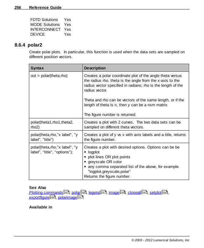
Reference Guide256
© 2003 - 2012 Lumerical Solutions, Inc
FDTD SolutionsMODE SolutionsINTERCONNECTDEVICE
YesYesYesYes
8.6.4 polar2
Create polar plots. In particular, this function is used when the data sets are sampled ondifferent position vectors.
Syntax Description
out = polar(theta,rho) Creates a polar coordinate plot of the angle theta versusthe radius rho. theta is the angle from the x-axis to theradius vector specified in radians; rho is the length of theradius vector.
Theta and rho can be vectors of the same length, or if thelength of theta is n, then y can be a nxm matrix.
The figure number is returned.
polar(theta1,rho1,theta2,rho2)
Creates a plot with 2 curves. The two data sets can besampled on different theta vectors.
polar(theta,rho,"x label", "ylabel", "title")
Creates a plot of y vs x with axis labels and a title, returnsthe figure number.
polar(theta,rho,"x label", "ylabel", "title", "options");
Creates a plot with desired options. Options can be be logplot plot lines OR plot points greyscale OR colorany comma separated list of the above, for example"logplot,greyscale,polar"
Returns the figure number.
See Also Plotting commands , polar , legend , image , closeall , setplot ,exportfigure , polarimage
Available in
252 255 257 258 261 260
260 257
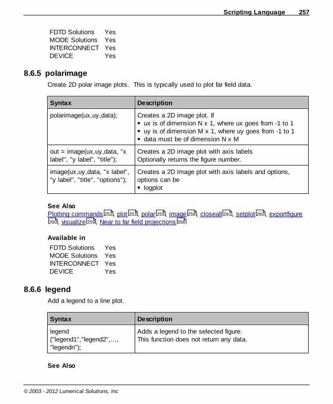
Scripting Language 257
© 2003 - 2012 Lumerical Solutions, Inc
FDTD SolutionsMODE SolutionsINTERCONNECTDEVICE
YesYesYesYes
8.6.5 polarimage
Create 2D polar image plots. This is typically used to plot far field data.
Syntax Description
polarimage(ux,uy,data); Creates a 2D image plot. If ux is of dimension N x 1, where ux goes from -1 to 1 uy is of dimension M x 1, where uy goes from -1 to 1 data must be of dimension N x M
out = image(ux,uy,data, "xlabel", "y label", "title");
Creates a 2D image plot with axis labelsOptionally returns the figure number.
image(ux,uy,data, "x label","y label", "title", "options");
Creates a 2D image plot with axis labels and options,options can be
logplot
See Also Plotting commands , plot , polar , image , closeall , setplot , exportfigure
, visualize , Near to far field projections
Available in
FDTD SolutionsMODE SolutionsINTERCONNECTDEVICE
YesYesYesYes
8.6.6 legend
Add a legend to a line plot.
Syntax Description
legend("legend1","legend2",...,"legendn");
Adds a legend to the selected figure.This function does not return any data.
See Also
252 253 255 258 261 260
260 259 358

Reference Guide258
© 2003 - 2012 Lumerical Solutions, Inc
Plotting commands , legend , plot , closeall , visualize
Available in
FDTD SolutionsMODE SolutionsINTERCONNECTDEVICE
YesYesYesYes
8.6.7 image
Create 2D image plots.
Syntax Description
out = image(x,y,z); Creates a 2D image plot. If x is of dimension N x 1 y is of dimension M x 1 z must be of dimension N x M
Returns the figure number.
image(x,y,z, "x label", "ylabel", "title");
Creates a 2D image plot with axis labels, returns the figurenumber.
image(x,y,z, "x label", "ylabel", "title", "options");
Creates a 2D image plot with axis labels and options,options can be
logplot polar any comma separated list of the above
See Also Plotting commands , plot , closeall , setplot , exportfigure , visualize ,polarimage
Available in
FDTD SolutionsMODE SolutionsINTERCONNECTDEVICE
YesYesYesYes
252 257 253 261 259
252 253 261 260 260 259
257
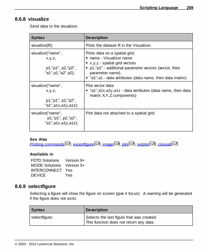
Scripting Language 259
© 2003 - 2012 Lumerical Solutions, Inc
8.6.8 visualize
Send data to the visualizer.
Syntax Description
visualize(R); Plots the dataset R in the Visualizer.
visualize("name", x,y,z, p1,"p1", p2,"p2", "a1",a1,"a2",a2);
Plots data on a spatial grid.name - Visualizer namex,y,z - spatial grid vectorsp1,"p1" - additional parameter vectors (vector, thenparameter name)."a1",a1 - data attributes (data name, then data matrix)
visualize("name", x,y,z, p1,"p1", p2,"p2", "a1",a1x,a1y,a1z);
Plot vector data "a1",a1x,a1y,a1z - data attributes (data name, then datamatrix X,Y,Z components)
visualize("name", p1,"p1", p2,"p2", "a1",a1x,a1y,a1z);
Plot data not attached to a spatial grid.
See Also Plotting commands , exportfigure , image , plot , setplot , closeall
Available in
FDTD SolutionsMODE SolutionsINTERCONNECTDEVICE
Version 8+Version 5+YesYes
8.6.9 selectfigure
Selecting a figure will show the figure on screen (give it focus). A warning will be generatedif the figure does not exist.
Syntax Description
selectfigure; Selects the last figure that was created.This function does not return any data.
252 260 258 253 260 261
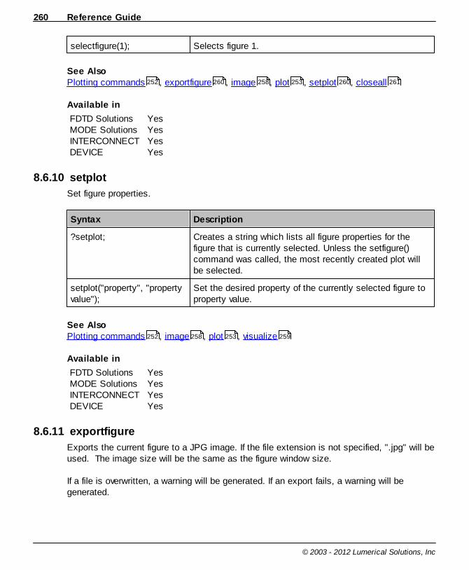
Reference Guide260
© 2003 - 2012 Lumerical Solutions, Inc
selectfigure(1); Selects figure 1.
See Also Plotting commands , exportfigure , image , plot , setplot , closeall
Available in
FDTD SolutionsMODE SolutionsINTERCONNECTDEVICE
YesYesYesYes
8.6.10 setplot
Set figure properties.
Syntax Description
?setplot; Creates a string which lists all figure properties for thefigure that is currently selected. Unless the setfigure()command was called, the most recently created plot willbe selected.
setplot("property", "propertyvalue");
Set the desired property of the currently selected figure toproperty value.
See Also Plotting commands , image , plot , visualize
Available in
FDTD SolutionsMODE SolutionsINTERCONNECTDEVICE
YesYesYesYes
8.6.11 exportfigure
Exports the current figure to a JPG image. If the file extension is not specified, ".jpg" will beused. The image size will be the same as the figure window size.
If a file is overwritten, a warning will be generated. If an export fails, a warning will begenerated.
252 260 258 253 260 261
252 258 253 259
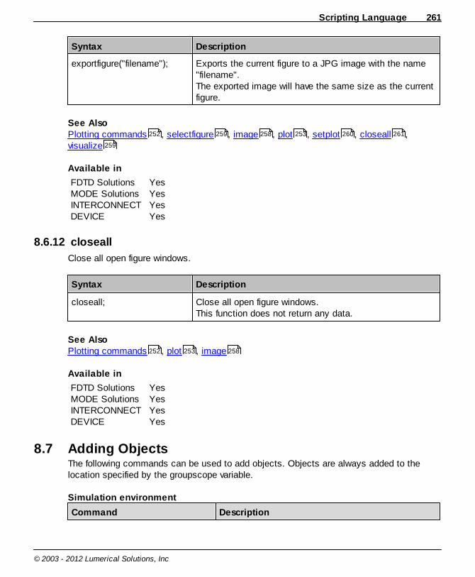
Scripting Language 261
© 2003 - 2012 Lumerical Solutions, Inc
Syntax Description
exportfigure("filename"); Exports the current figure to a JPG image with the name"filename".The exported image will have the same size as the currentfigure.
See Also Plotting commands , selectfigure , image , plot , setplot , closeall ,visualize
Available in
FDTD SolutionsMODE SolutionsINTERCONNECTDEVICE
YesYesYesYes
8.6.12 closeall
Close all open figure windows.
Syntax Description
closeall; Close all open figure windows.This function does not return any data.
See Also Plotting commands , plot , image
Available in
FDTD SolutionsMODE SolutionsINTERCONNECTDEVICE
YesYesYesYes
8.7 Adding ObjectsThe following commands can be used to add objects. Objects are always added to thelocation specified by the groupscope variable.
Simulation environment
Command Description
252 259 258 253 260 261
259
252 253 258
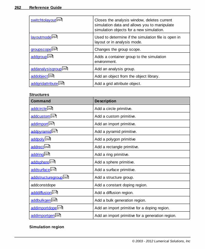
Reference Guide262
© 2003 - 2012 Lumerical Solutions, Inc
switchtolayout Closes the analysis window, deletes currentsimulation data and allows you to manipulatesimulation objects for a new simulation.
layoutmode Used to determine if the simulation file is open inlayout or in analysis mode.
groupscope Changes the group scope.
addgroup Adds a container group to the simulationenvironment.
addanalysisgroup Add an analysis group.
addobject Add an object from the object library.
addgridattribute Add a grid attribute object.
Structures
Command Description
addcircle Add a circle primitive.
addcustom Add a custom primitive.
addimport Add an import primitive.
addpyramid Add a pyramid primitive.
addpoly Add a polygon primitive
addrect Add a rectangle primitive.
addring Add a ring primitive.
addsphere Add a sphere primitive.
addsurface Add a surface primitive.
addstructuregroup Add a structure group.
addconstdope Add a constant doping region.
adddiffusion Add a diffusion region.
addbulkgen Add a bulk generation region.
addimportdope Add an import primitive for a doping region.
addimportgen Add an import primitive for a generation region.
Simulation region
264
264
284
264
265
266
280
266
267
267
267
268
268
269
270
270
265
279
280
279
280

Scripting Language 263
© 2003 - 2012 Lumerical Solutions, Inc
Command Description
addfdtd Add an FDTD simulation area.
addeigenmode Adds a MODE simulation area.
addpropagator Adds a propagator simulation object to the MODESolutions simulation environment.
addmesh Add a mesh override region.
adddevice Adds a DEVICE simulation area.
Sources
Command Description
adddipole Add a dipole source.
addgaussian Add a Gaussian source.
addplane Add a plane source.
addmode ; addmodesource Add a mode source.
addtfsf Add a TFSF source.
addimportedsource Add an imported source.
Monitors
Command Description
addindex Add an index monitor.
addtime Add a time monitor.
addmovie Add a movie monitor.
addprofile Add a profile monitor.
addpower Add a power monitor.
Create objects in Deck
Command Description
createbeam Creates a new Gaussian beam that is accessiblefrom the deck.
270
271
271
272
278
273
273
274
272 273
274
275
275
276
276
276
277
277

Reference Guide264
© 2003 - 2012 Lumerical Solutions, Inc
8.7.1 switchtolayout
Closes the analysis window and allows you to manipulate simulation objects for a newsimulation. If a simulation file is open in ANALYSIS mode, any commands to modifyobjects will return errors. You must switch to LAYOUT mode before modifying any ob jects.
Syntax Description
switchtolayout; Switches to LAYOUT mode.This function does not return any data.
See AlsoAdding Objects , layoutmode
Available in
FDTD SolutionsMODE SolutionsINTERCONNECTDEVICE
YesYesYesYes
8.7.2 layoutmode
Used to determine if the simulation file is open in layout or in analysis mode.
Syntax Description
?layoutmode; Returns 1 if in layout mode, and 0 if in analysis mode.
See AlsoAdding Objects , switchtolayout
Available in
FDTD SolutionsMODE SolutionsINTERCONNECTDEVICE
YesYesYesYes
8.7.3 addgroup
Adds a container group to the simulation environment.
Syntax Description
261 264
261 264
Scripting Language 265
© 2003 - 2012 Lumerical Solutions, Inc
addgroup; Adds a container group to the simulation environment.This function does not return any data.
See AlsoAdding Objects , addtogroup , addstructuregroup , addanalysisgroup
Available in
FDTD SolutionsMODE SolutionsINTERCONNECTDEVICE
YesYesNoYes
8.7.4 addstructuregroup
Adds a structure group to the simulation environment.
Syntax Description
addstructuregroup; Adds a structure group to the simulation environment.This function does not return any data.
See AlsoAdding Objects , addtogroup , adduserprop , addgroup , addanalysisgroup
Available in
FDTD SolutionsMODE SolutionsINTERCONNECTDEVICE
YesYesNoYes
8.7.5 addanalysisgroup
Adds an analysis group to the simulation environment.
Syntax Description
addanalysisgroup; Adds an analysis group to the simulation environment.This function does not return any data.
See AlsoAdding Objects , addtogroup , adduserprop , addgroup , addstructuregroup
Available in
261 290 265 265
261 290 291 264 265
261 290 291 264 265
Reference Guide266
© 2003 - 2012 Lumerical Solutions, Inc
FDTD SolutionsMODE SolutionsINTERCONNECTDEVICE
YesYesNoYes
8.7.6 addobject
Adds a object from the object library. T
Syntax Description
addobject("script_ID"); Adds an object from the object library.This function does not return any data.
See AlsoAdding Objects , addtogroup , adduserprop
Available in
FDTD SolutionsMODE SolutionsINTERCONNECTDEVICE
YesYesNoNo
8.7.7 addcircle
Adds a circle primitive to the simulation environment.
Syntax Description
addcircle; Adds primitive to the simulation environment.This function does not return any data.
See AlsoAdding Objects
Available in
FDTD SolutionsMODE SolutionsINTERCONNECTDEVICE
YesYesNoYes
asdd
261 290 291
261
Scripting Language 267
© 2003 - 2012 Lumerical Solutions, Inc
8.7.8 addcustom
Adds a custom primitive to the simulation environment.
Syntax Description
addcustom; Adds primitive to the simulation environment.This function does not return any data.
See AlsoAdding Objects
Available in
FDTD SolutionsMODE SolutionsINTERCONNECTDEVICE
YesYesNoNo
8.7.9 addimport
Adds an import primitive to the simulation environment.
Syntax Description
addimport; Adds primitive to the simulation environment.This function does not return any data.
See AlsoAdding Objects
Available in
FDTD SolutionsMODE SolutionsINTERCONNECTDEVICE
YesYesNoNo
8.7.10 addpyramid
Adds a pyramid primitive to the simulation environment.
Syntax Description
addpyramid; Adds primitive to the simulation environment.
261
261
Reference Guide268
© 2003 - 2012 Lumerical Solutions, Inc
This function does not return any data.
See AlsoAdding Objects
Available in
FDTD SolutionsMODE SolutionsINTERCONNECTDEVICE
YesYesNoYes
8.7.11 addpoly
Adds a polygon primitive to the simulation environment.
Syntax Description
addpoly; Adds primitive to the simulation environment.This function does not return any data.
See AlsoAdding Objects
Available in
FDTD SolutionsMODE SolutionsINTERCONNECTDEVICE
YesYesNoYes
8.7.12 addrect
Adds a rectangle primitive to the simulation environment.
Syntax Description
addrect; Adds primitive to the simulation environment.This function does not return any data.
See AlsoAdding Objects
Available in
261
261
261

Scripting Language 269
© 2003 - 2012 Lumerical Solutions, Inc
FDTD SolutionsMODE SolutionsINTERCONNECTDEVICE
YesYesNoYes
8.7.13 addtriangle
Adds a 3 vertex, triangle shaped polygon primitive to the simulation environment.
Syntax Description
addtriangle; Adds primitive to the simulation environment.This function does not return any data.
See AlsoAdding Objects , addpoly
Available in
FDTD SolutionsMODE SolutionsINTERCONNECTDEVICE
YesYesNoYes
8.7.14 addring
Adds a ring primitive to the simulation environment.
Syntax Description
addring; Adds primitive to the simulation environment.This function does not return any data.
See AlsoAdding Objects
Available in
FDTD SolutionsMODE SolutionsINTERCONNECTDEVICE
YesYesNoYes
261 268
261
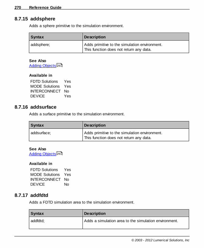
Reference Guide270
© 2003 - 2012 Lumerical Solutions, Inc
8.7.15 addsphere
Adds a sphere primitive to the simulation environment.
Syntax Description
addsphere; Adds primitive to the simulation environment.This function does not return any data.
See AlsoAdding Objects
Available in
FDTD SolutionsMODE SolutionsINTERCONNECTDEVICE
YesYesNoYes
8.7.16 addsurface
Adds a surface primitive to the simulation environment.
Syntax Description
addsurface; Adds primitive to the simulation environment.This function does not return any data.
See AlsoAdding Objects
Available in
FDTD SolutionsMODE SolutionsINTERCONNECTDEVICE
YesYesNoNo
8.7.17 addfdtd
Adds a FDTD simulation area to the simulation environment.
Syntax Description
addfdtd; Adds a simulation area to the simulation environment.
261
261

Scripting Language 271
© 2003 - 2012 Lumerical Solutions, Inc
This function does not return any data.
See AlsoAdding Objects
Available in
FDTD SolutionsMODE SolutionsINTERCONNECTDEVICE
YesYesNoNo
8.7.18 addeigenmode
Adds an eigenmode simulation object to the MODE Solutions simulation environment.
Syntax Description
addeigenmode; Add an eigenmode mode simulation region.
See AlsoAdding Objects
Available in
FDTD SolutionsMODE SolutionsINTERCONNECTDEVICE
NoYesNoNo
8.7.19 addpropagator
Adds a propagator simulation object to the MODE Solutions simulation environment.
Syntax Description
addpropagator; Add a propagator mode simulation region.
See AlsoAdding Objects
Available in
261
261
261
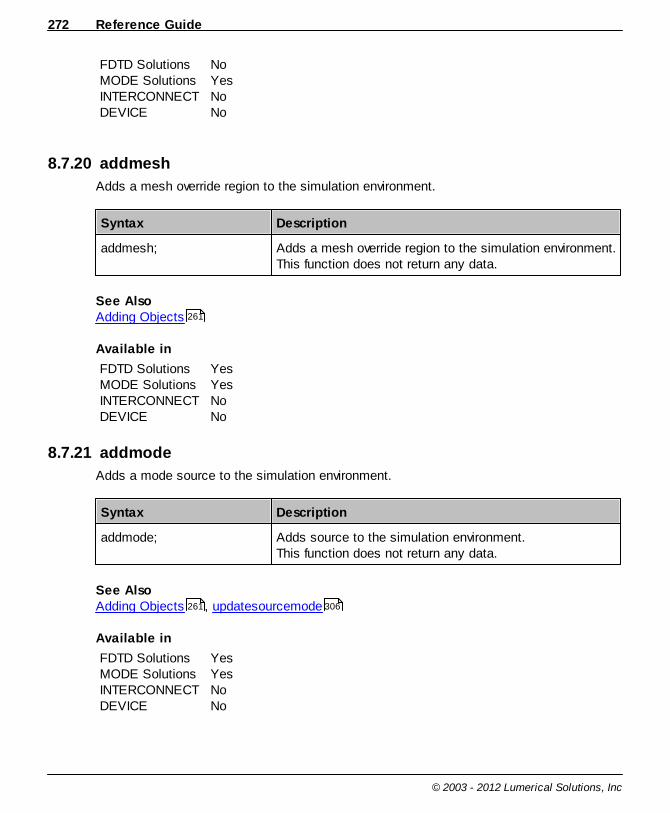
Reference Guide272
© 2003 - 2012 Lumerical Solutions, Inc
FDTD SolutionsMODE SolutionsINTERCONNECTDEVICE
NoYesNoNo
8.7.20 addmesh
Adds a mesh override region to the simulation environment.
Syntax Description
addmesh; Adds a mesh override region to the simulation environment.This function does not return any data.
See AlsoAdding Objects
Available in
FDTD SolutionsMODE SolutionsINTERCONNECTDEVICE
YesYesNoNo
8.7.21 addmode
Adds a mode source to the simulation environment.
Syntax Description
addmode; Adds source to the simulation environment.This function does not return any data.
See AlsoAdding Objects , updatesourcemode
Available in
FDTD SolutionsMODE SolutionsINTERCONNECTDEVICE
YesYesNoNo
261
261 306
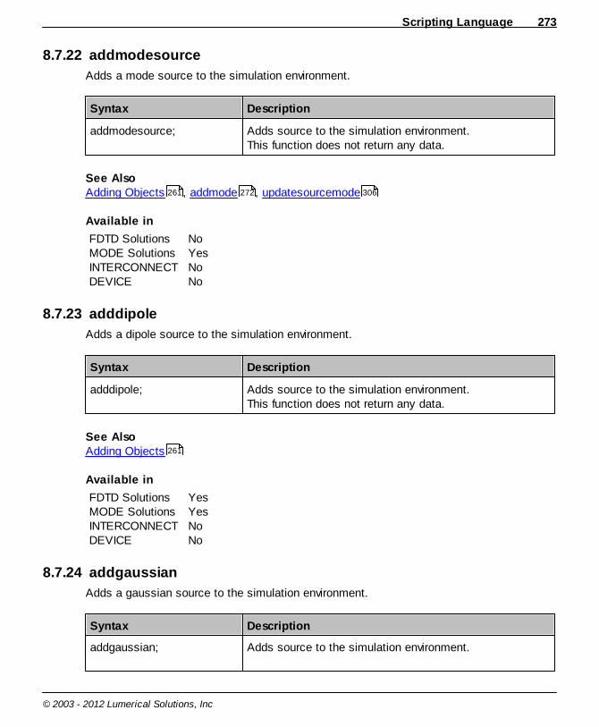
Scripting Language 273
© 2003 - 2012 Lumerical Solutions, Inc
8.7.22 addmodesource
Adds a mode source to the simulation environment.
Syntax Description
addmodesource; Adds source to the simulation environment.This function does not return any data.
See AlsoAdding Objects , addmode , updatesourcemode
Available in
FDTD SolutionsMODE SolutionsINTERCONNECTDEVICE
NoYesNoNo
8.7.23 adddipole
Adds a dipole source to the simulation environment.
Syntax Description
adddipole; Adds source to the simulation environment.This function does not return any data.
See AlsoAdding Objects
Available in
FDTD SolutionsMODE SolutionsINTERCONNECTDEVICE
YesYesNoNo
8.7.24 addgaussian
Adds a gaussian source to the simulation environment.
Syntax Description
addgaussian; Adds source to the simulation environment.
261 272 306
261

Reference Guide274
© 2003 - 2012 Lumerical Solutions, Inc
This function does not return any data.
See AlsoAdding Objects
Available in
FDTD SolutionsMODE SolutionsINTERCONNECTDEVICE
YesYesNoNo
8.7.25 addplane
Adds a plane wave source to the simulation environment.
Syntax Description
addplane; Adds source to the simulation environment.This function does not return any data.
See AlsoAdding Objects
Available in
FDTD SolutionsMODE SolutionsINTERCONNECTDEVICE
YesYesNoNo
8.7.26 addtfsf
Adds a Total Field Scattered Field (tfsf) source to the simulation environment.
Syntax Description
addtfsf; Adds source to the simulation environment.This function does not return any data.
See AlsoAdding Objects
Available in
261
261
261

Scripting Language 275
© 2003 - 2012 Lumerical Solutions, Inc
FDTD SolutionsMODE SolutionsINTERCONNECTDEVICE
YesYesNoNo
8.7.27 addimportedsource
Adds an imported source to the simulation environment.
Syntax Description
addimportedsource; Adds source to the simulation environment.This function does not return any data.
See AlsoAdding Objects , asapimport , asapload , asapexport
Available in
FDTD SolutionsMODE SolutionsINTERCONNECTDEVICE
YesNoNoNo
8.7.28 addindex
Adds an index monitor to the simulation environment.
Syntax Description
addindex; Adds monitor to the simulation environment.This function does not return any data.
See AlsoAdding Objects
Available in
FDTD SolutionsMODE SolutionsINTERCONNECTDEVICE
YesYesNoNo
261 177 176 176
261

Reference Guide276
© 2003 - 2012 Lumerical Solutions, Inc
8.7.29 addtime
Adds a time monitor to the simulation environment.
Syntax Description
addtime; Adds monitor to the simulation environment.This function does not return any data.
See AlsoAdding Objects
Available in
FDTD SolutionsMODE SolutionsINTERCONNECTDEVICE
YesYesNoNo
8.7.30 addmovie
Adds a movie monitor to the simulation environment.
Syntax Description
addmovie; Adds monitor to the simulation environment.This function does not return any data.
See AlsoAdding Objects
Available in
FDTD SolutionsMODE SolutionsINTERCONNECTDEVICE
YesYesNoNo
8.7.31 addprofile
Adds a profile monitor to the simulation environment.
Syntax Description
addprofile; Adds monitor to the simulation environment.
261
261

Scripting Language 277
© 2003 - 2012 Lumerical Solutions, Inc
This function does not return any data.
See AlsoAdding Objects
Available in
FDTD SolutionsMODE SolutionsINTERCONNECTDEVICE
YesYesNoNo
8.7.32 addpower
Adds a power monitor to the simulation environment.
Syntax Description
addpower; Adds monitor to the simulation environment.This function does not return any data.
See AlsoAdding Objects
Available in
FDTD SolutionsMODE SolutionsINTERCONNECTDEVICE
YesYesNoNo
8.7.33 createbeam
Creates a new Gaussian beam that is accessible from the deck.
Only available in MODE Solutions.
Syntax Description
createbeam; Creates a Gaussian beam in the deck/global workspace.The Gaussian beam has the properties specified in theOverlap analysis->Beam tab of the analysis windowReturns the name of the Gaussian beam created, which isby default "gaussian#" (# being the total number ofGaussian beams existing in the current deck).
261
261
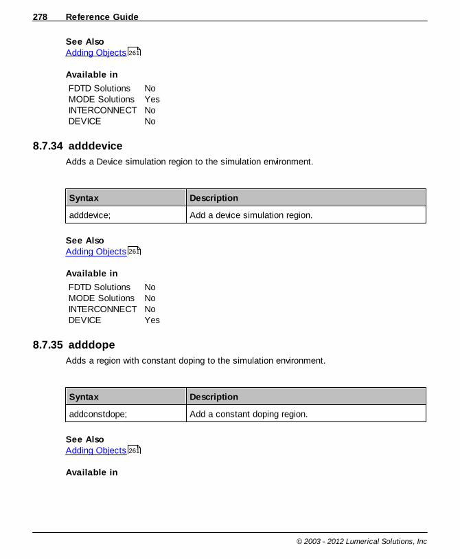
Reference Guide278
© 2003 - 2012 Lumerical Solutions, Inc
See AlsoAdding Objects
Available in
FDTD SolutionsMODE SolutionsINTERCONNECTDEVICE
NoYesNoNo
8.7.34 adddevice
Adds a Device simulation region to the simulation environment.
Syntax Description
adddevice; Add a device simulation region.
See Also Adding Objects
Available in
FDTD SolutionsMODE SolutionsINTERCONNECTDEVICE
NoNoNoYes
8.7.35 adddope
Adds a region with constant doping to the simulation environment.
Syntax Description
addconstdope; Add a constant doping region.
See Also Adding Objects
Available in
261
261
261

Scripting Language 279
© 2003 - 2012 Lumerical Solutions, Inc
FDTD SolutionsMODE SolutionsINTERCONNECTDEVICE
NoNoNoYes
8.7.36 adddiffusion
Adds a diffusion region to the simulation environment.
Syntax Description
adddiffusion; Add a diffusion region.
See Also Adding Objects
Available in
FDTD SolutionsMODE SolutionsINTERCONNECTDEVICE
NoNoNoYes
8.7.37 addimportdope
Adds a doping region to the simulation environment where the doping profile has been orwill be imported into DEVICE.
Syntax Description
addimportdope; Add an import primitive to define a doping region.
See Also Adding Objects
Available in
FDTD SolutionsMODE SolutionsINTERCONNECTDEVICE
NoNoNoYes
261
261

Reference Guide280
© 2003 - 2012 Lumerical Solutions, Inc
8.7.38 addbulkgen
Adds a bulk generation region to the simulation environment.
Syntax Description
addbulkgen; Add a bulk generation region.
See Also Adding Objects
Available in
FDTD SolutionsMODE SolutionsINTERCONNECTDEVICE
NoNoNoYes
8.7.39 addimportgen
Adds a generation region to the simulation environment where the generation profile hasbeen imported into DEVICE.
Syntax Description
addimportgen; Add an import primitive to define a generation region.
See Also Adding Objects
Available in
FDTD SolutionsMODE SolutionsINTERCONNECTDEVICE
NoNoNoYes
8.7.40 addgridattribute
Adds a grid attribute object to the simulation environment.
Syntax Description
261
261
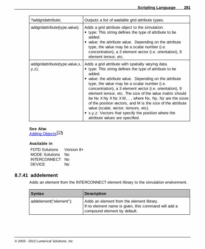
Scripting Language 281
© 2003 - 2012 Lumerical Solutions, Inc
?addgridattribute; Outputs a list of available grid attribute types.
addgridattribute(type,value); Adds a grid attribute object to the simulation.type: This string defines the type of attribute to beadded. value: the attribute value. Depending on the attributetype, the value may be a scalar number (i.e.concentration), a 3 element vector (i.e. orientation), 9element tensor, etc.
addgridattribute(type,value,x,y,z);
Adds a grid attribute with spatially varying data.type: This string defines the type of attribute to beadded. value: the attribute value. Depending on the attributetype, the value may be a scalar number (i.e.concentration), a 3 element vector (i.e. orientation), 9element tensor, etc. The size of the value matrix shouldbe Nx X Ny X Nz X M… , where Nx, Ny, Nz are the sizesof the position vectors, and M is the size of the attributevalue (scalar, vector, tensors, etc). x,y,z: Vectors that specify the position where theattribute values are specified.
See Also Adding Objects
Available in
FDTD SolutionsMODE SolutionsINTERCONNECTDEVICE
Version 8+NoNoNo
8.7.41 addelement
Adds an element from the INTERCONNECT element library to the simulation environment.
Syntax Description
addelement("element"); Adds an element from the element library.If no element name is given, this command will add acompound element by default.
261
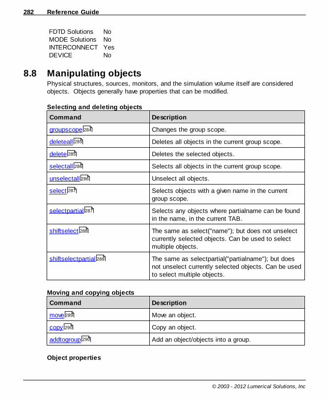
Reference Guide282
© 2003 - 2012 Lumerical Solutions, Inc
FDTD SolutionsMODE SolutionsINTERCONNECTDEVICE
NoNoYesNo
8.8 Manipulating objectsPhysical structures, sources, monitors, and the simulation volume itself are consideredobjects. Objects generally have properties that can be modified.
Selecting and deleting objects
Command Description
groupscope Changes the group scope.
deleteall Deletes all objects in the current group scope.
delete Deletes the selected objects.
selectall Selects all objects in the current group scope.
unselectall Unselect all objects.
select Selects objects with a given name in the currentgroup scope.
selectpartial Selects any objects where partialname can be foundin the name, in the current TAB.
shiftselect The same as select("name"); but does not unselectcurrently selected objects. Can be used to selectmultiple objects.
shiftselectpartial The same as selectpartial("partialname"); but doesnot unselect currently selected objects. Can be usedto select multiple objects.
Moving and copying objects
Command Description
move Move an object.
copy Copy an object.
addtogroup Add an object/objects into a group.
Object properties
284
285
285
286
286
287
287
288
289
289
290
290

Scripting Language 283
© 2003 - 2012 Lumerical Solutions, Inc
Command Description
adduserprop Add a user property to a structure group.
set Set a property of selected objects.
setnamed Set a property of any objects with a given name.
setglobalmonitor Set global monitor properties.
setglobalsource Set global source properties.
runsetup Force group setup scripts to run.
get Get a property of selected objects.
getnumber Get the number of selected objects.
getnamed Get a property of any objects with a given name.
getnamednumber Get the number of objects with a given name.
getglobalmonitor Get global monitor properties.
getglobalsource Get global source properties.
haveproperty Returns the number of selected objects with aparticular property.
importsurface Import surface data from a file. Only applies to importprimitives.
importsurface2 Import surface data from script variables. Onlyapplies to import primitives.
importnk Import n and k data from a file. Only applies to importprimitives.
importnk2 Import n and k data from script variables. Onlyapplies to import primitives.
setsourcesignal Set a custom source time signal.
updatesourcemode Updates the mode for a mode source.
clearsourcedata Clears source data for an imported source, or theselected mode for a mode source.
Controlling the view
Command Description
redraw Redraw graphics.
291
292
292
293
294
295
294
296
296
297
298
298
299
300
301
302
304
305
306
307
307
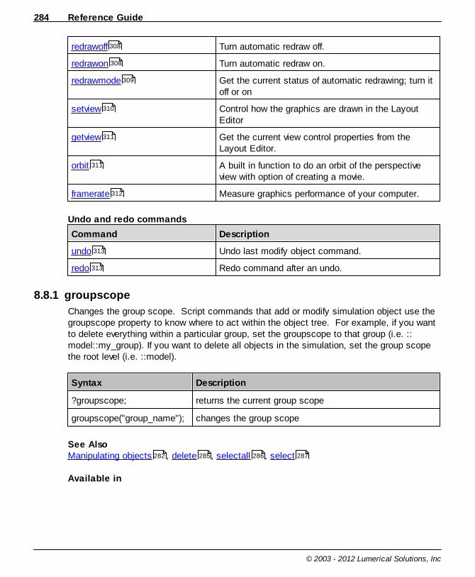
Reference Guide284
© 2003 - 2012 Lumerical Solutions, Inc
redrawoff Turn automatic redraw off.
redrawon Turn automatic redraw on.
redrawmode Get the current status of automatic redrawing; turn itoff or on
setview Control how the graphics are drawn in the LayoutEditor
getview Get the current view control properties from theLayout Editor.
orbit A built in function to do an orbit of the perspectiveview with option of creating a movie.
framerate Measure graphics performance of your computer.
Undo and redo commands
Command Description
undo Undo last modify object command.
redo Redo command after an undo.
8.8.1 groupscope
Changes the group scope. Script commands that add or modify simulation object use thegroupscope property to know where to act within the object tree. For example, if you wantto delete everything within a particular group, set the groupscope to that group (i.e. ::model::my_group). If you want to delete all objects in the simulation, set the group scopethe root level (i.e. ::model).
Syntax Description
?groupscope; returns the current group scope
groupscope("group_name"); changes the group scope
See Also Manipulating objects , delete , selectall , select
Available in
308
308
309
310
311
311
312
313
313
282 285 286 287
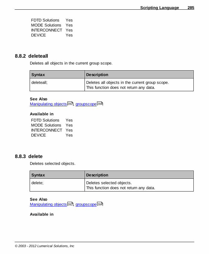
Scripting Language 285
© 2003 - 2012 Lumerical Solutions, Inc
FDTD SolutionsMODE SolutionsINTERCONNECTDEVICE
YesYesYesYes
8.8.2 deleteall
Deletes all objects in the current group scope.
Syntax Description
deleteall; Deletes all objects in the current group scope.This function does not return any data.
See Also Manipulating objects , groupscope
Available in
FDTD SolutionsMODE SolutionsINTERCONNECTDEVICE
YesYesYesYes
8.8.3 delete
Deletes selected objects.
Syntax Description
delete; Deletes selected objects.This function does not return any data.
See Also Manipulating objects , groupscope
Available in
282 284
282 284
Reference Guide286
© 2003 - 2012 Lumerical Solutions, Inc
FDTD SolutionsMODE SolutionsINTERCONNECTDEVICE
YesYesYesYes
8.8.4 selectall
Selects all objects in the current group scope.
Syntax Description
selectall; Selects all objects in the current group scope.This function does not return any data.
See Also Manipulating objects , groupscope
Available in
FDTD SolutionsMODE SolutionsINTERCONNECTDEVICE
YesYesYesYes
8.8.5 unselectall
Unselect all objects and groups.
Syntax Description
unselectall; Unselects all objects and groups.This function does not return any data.
See Also Manipulating objects
Available in
282 284
282

Scripting Language 287
© 2003 - 2012 Lumerical Solutions, Inc
FDTD SolutionsMODE SolutionsINTERCONNECTDEVICE
YesYesYesYes
8.8.6 select
Selects objects with a given name in the current group scope. A failed select command willhave the same result as the unselectall command.
Syntax Description
select("name"); Selects objects with the name "name" in the current groupscope. This function does not return any data.
select("group name::name"); Selects all objects with the name "name" located in thegroup named "group name". The group named "groupname" must be in the current group scope.
See Also Manipulating objects , groupscope , unselectall
Available in
FDTD SolutionsMODE SolutionsINTERCONNECTDEVICE
YesYesYesYes
8.8.7 selectpartial
Selects any objects with a given partial name, in the current TAB.
Syntax Description
selectpartial("partialname"); Selects any objects where "partialname" can be found inthe object name provided the object is not in a group. Toselect objects located in groups see the command below.This function does not return any data.
282 284 286
Reference Guide288
© 2003 - 2012 Lumerical Solutions, Inc
selectpartial("partialgroupname::partialname");
Selects any objects where "partialgroupname" can befound in the group name and "partialname" can be found inthe object name.
See Also Manipulating objects , groupscope
Available in
FDTD SolutionsMODE SolutionsINTERCONNECTDEVICE
YesYesYesYes
8.8.8 shiftselect
Same as select, but does not unselect other currently selected objects.
Syntax Description
shiftselect("name"); The same as select("name"), but does not unselectcurrently selected objects. Can be used to select multipleobjects.This function does not return any data.
shiftselect("group name::name");
The same as select("groupname::name"), but does notunselect currently selected objects.
See Also Manipulating objects , groupscope
Available in
FDTD SolutionsMODE SolutionsINTERCONNECTDEVICE
YesYesYesYes
282 284
282 284

Scripting Language 289
© 2003 - 2012 Lumerical Solutions, Inc
8.8.9 shiftselectpartial
Same as selectpartial, but does not unselect other currently selected objects.
Syntax Description
shiftselectpartial("partialname");
The same as selectpartial("partialname"), but does notunselect currently selected objects. Can be used to selectmultiple objects. This function does not return any data.
shiftselectpartial("partialgroupname::partialname");
The same as selectpartial("partialgroupname::partialname"), but does not unselect currently selected objects. Can beused to select multiple objects.
See Also Manipulating objects , groupscope
Available in
FDTD SolutionsMODE SolutionsINTERCONNECTDEVICE
YesYesYesYes
8.8.10 move
Move selected objects.
Syntax Description
move(dx); In 2D or 3D, move by dx
move(dx,dy); In 2D or 3D, move by dx and dy.This function does not return any data.
move(dx,dy,dz); In 3D, move by dx, dy, and dz.In 2D, dz will be ignored.
See Also Manipulating objects , copy , select
Available in
282 284
282 290 287
Reference Guide290
© 2003 - 2012 Lumerical Solutions, Inc
FDTD SolutionsMODE SolutionsINTERCONNECTDEVICE
YesYesYesYes
8.8.11 copy
Copy selected objects.
Syntax Description
copy; Copy the selected objects. The new objects will have havethe same name. Their position will be shifted by a defaultamount.This function does not return any data.
copy(dx); Same as copy; but with a specified move of dx.
copy(dx,dy); Same as copy; but with a specified move of dx, dy.
copy(dx,dy,dz); Same as copy; but with a specified move of dx, dy, dz. In 2D, dz is ignored.
See Also Manipulating objects , move , select , cp (copy files)
Available in
FDTD SolutionsMODE SolutionsINTERCONNECTDEVICE
YesYesYesYes
8.8.12 addtogroup
Add selected objects to a group.
Syntax Description
addtogroup("group name"); Adds selected object(s) to a group. If a group with name"group name" already exists, then the objects are added tothe existing group. Otherwise, a group named "group
282 289 287 164
Scripting Language 291
© 2003 - 2012 Lumerical Solutions, Inc
name" is created.This function does not return any data.
See AlsoManipulating objects , addgroup , addstructuregroup , addanalysisgroup ,adduserprop , runsetup
Available in
FDTD SolutionsMODE SolutionsINTERCONNECTDEVICE
YesYesNoYes
8.8.13 adduserprop
Add user properties to a structure group.
Syntax Description
adduserprop("propertyname", type, value);
Adds a user property to a selected structure group. Thename is set to "property name". The type is an integerfrom 0 to 5. The corresponding variable types are0 number1 text2 length3 time 4 frequency5 materialThe value of the user property is set to value.
See AlsoManipulating objects , addstructuregroup , runsetup
Available in
FDTD SolutionsMODE SolutionsINTERCONNECTDEVICE
YesYesNoYes
282 264 265 265
291 295
282 265 295

Reference Guide292
© 2003 - 2012 Lumerical Solutions, Inc
8.8.14 set
Set a property of currently selected objects. This command will return an error in analysismode.
Syntax Description
?set; Returns a list of the properties of the selected object(s).
set("property",value); This will set the properties of a currently selected object,including pull-downs and check boxes. It cannot be usedto set the value of a selected object in a group. Value can be a number or string. This function does notreturn any data.
set("property",value,i); This form can be used to set the property of the ithselected object when multiple objects are selected. Itcannot be used to set the value of a selected object in agroup. The objects are ordered by their location in the object tree.The uppermost selected object is given the index 1, andthe index numbers increase as you go down the tree.
See Also Manipulating objects , get , setnamed , setmaterial , addmaterial ,haveproperty , runsetup , runanalysis
Available in
FDTD SolutionsMODE SolutionsINTERCONNECTDEVICE
YesYesYesYes
8.8.15 setnamed
Like the set command, except that the object name must be specified. This command willreturn an error in analysis mode.
Syntax Description
?setnamed("name"); Returns a list of the properties of the objects called name.
setnamed("name","property", value);
The same as set, but acts on objects with a specificname, instead of selected objects.
282 294 292 387 386
299 295 350
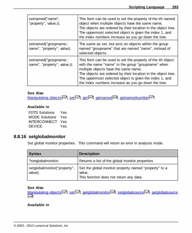
Scripting Language 293
© 2003 - 2012 Lumerical Solutions, Inc
setnamed("name","property", value,i);
This form can be used to set the property of the ith namedobject when multiple objects have the same name. The objects are ordered by their location in the object tree.The uppermost selected object is given the index 1, andthe index numbers increase as you go down the tree.
setnamed("groupname::name", "property", value);
The same as set, but acts on objects within the groupnamed "groupname" that are named "name", instead ofselected objects.
setnamed("groupname::name", "property", value,i);
This form can be used to set the property of the ith objectwith the name "name" in the group "groupname" whenmultiple objects have the same name. The objects are ordered by their location in the object tree.The uppermost selected object is given the index 1, andthe index numbers increase as you go down the tree.
See Also Manipulating objects , set , get , getnamed , getnamednumber
Available in
FDTD SolutionsMODE SolutionsINTERCONNECTDEVICE
YesYesYesYes
8.8.16 setglobalmonitor
Set global monitor properties. This command will return an error in analysis mode.
Syntax Description
?setglobalmonitor; Returns a list of the global monitor properties
setglobalmonitor("property",value);
Set the global monitor property named "property" to avalue.This function does not return any data.
See Also Manipulating objects , set , getglobalmonitor , setglobalsource , getglobalsource
Available in
282 292 294 296 297
282 292 298 294
298

Reference Guide294
© 2003 - 2012 Lumerical Solutions, Inc
FDTD SolutionsMODE SolutionsINTERCONNECTDEVICE
YesYesNoNo
8.8.17 setglobalsource
Set global source properties. This command will return an error in analysis mode.
Syntax Description
?setglobalsource; Returns a list of the global source properties
setglobalsource("property",value);
Set the global source property named "property" to a value.This function does not return any data.
See Also Manipulating objects , set , setglobalmonitor , getglobalmonitor ,getglobalsource
Available in
FDTD SolutionsMODE SolutionsINTERCONNECTDEVICE
YesYesNoNo
8.8.18 get
Get a property from selected objects. The property names for the get command are thesame as the property names in the Edit dialogue box. For example, if you see a propertycalled "mesh accuracy", then you can use the command get("mesh accuracy"); to get thatproperty. It is possible to get numeric, string, drop down and checkbox properties.
Note: Beam profilesIn addition to the properties available through the Edit dialogue, it is possible to get thebeam profile for gaussian, planewave and mode sources. The property names are "xvector","y vector","z vector","Ex","Ey","Ez","Hx","Hy", and "Hz". In addition, for modesources, the real part of the effective index for the mode can be obtained. This property isnamed "neff".
282 292 293 298
298

Scripting Language 295
© 2003 - 2012 Lumerical Solutions, Inc
Syntax Description
?get; Returns a list of the properties of the selected object(s).
out = get("property"); Gets the requested property value from the currentlyselected object. It cannot be used to get the property valueof a selected object in a group. If multiple objects are selected get("property") is the sameas get("property",i), where i is the number of the firstselected objects with the requested property. Out can be a matrix or a string, depending on the propertyrequested.
get("property",i); Gets the property of the ith selected object. Use this to acton a series of objects. It cannot be used to get the value ofa selected object in a group. The objects are ordered by their location in the object tree.The uppermost selected object is given the index 1, andthe index numbers increase as you go down the tree.
See Also Manipulating objects , getnumber , getnamed , getnamednumber , set ,haveproperty , runsetup
Available in
FDTD SolutionsMODE SolutionsINTERCONNECTDEVICE
YesYesYesYes
8.8.19 runsetup
Runsetup forces the setup scripts of structure and analysis groups to run.
In most cases, it is not necessary to use this function, as group setup scriptsautomatically re-run at the end of script, if the object has been modified. It is onlynecessary to use this function when you need to force the setup script to run before theend of your script file.
Syntax Description
282 296 296 297 292
299 295

Reference Guide296
© 2003 - 2012 Lumerical Solutions, Inc
runsetup; Forces setup scripts of groups to run.
See Also Manipulating objects , get , set , runanalysis
Available in
FDTD SolutionsMODE SolutionsINTERCONNECTDEVICE
YesYesYesYes
8.8.20 getnumber
Get the number of objects that are selected.
Syntax Description
out = getnumber; Returns the number of objects that are selected;
See Also Manipulating objects , get , getnamed , getnamednumber , set
Available in
FDTD SolutionsMODE SolutionsINTERCONNECTDEVICE
YesYesYesYes
8.8.21 getnamed
Get a property from objects with a given name.
If multiple objects are selected, and the values are different, the smallest value is returned. To be certain of the results, be sure that only one object is selected, or use the form ofgetnamed that allows a specific object to be selected.
Syntax Description
?getnamed("name"); Returns a list of the properties of the objects called name.
282 294 292 350
282 294 296 297 292

Scripting Language 297
© 2003 - 2012 Lumerical Solutions, Inc
out = getnamed("name","property");
The same as get, but acts on objects with a specificname, instead of selected objects.
out=getnamed("name","property", i);
Gets the property of the ith named object. Use this to acton a series of objects.The objects are ordered by their location in the object tree.The uppermost selected object is given the index 1, andthe index numbers increase as you go down the tree.
out = getnamed("groupname::name","property");
The same as get, but acts on objects named "name"located in the group "groupname", instead of selectedobjects.
out = getnamed("groupname::name","property");
Gets the property of the ith object named "name" locatedin the group "groupname". Use this to act on a series ofobjects.The objects are ordered by their location in the object tree.The uppermost selected object is given the index 1, andthe index numbers increase as you go down the tree.
See Also Manipulating objects , get , getnumber , getnamednumber , set , setnamed
Available in
FDTD SolutionsMODE SolutionsINTERCONNECTDEVICE
YesYesYesYes
8.8.22 getnamednumber
Get the number of objects with a given name.
Syntax Description
out = getnamednumber( "name");
The same as getnumber, but acts on objects with aspecific name, instead of selected objects.
out = getnamednumber( "groupname::name");
The same as getnumber, but acts on all objects named"name" in the group "groupname", instead of selected
282 294 296 297 292
292
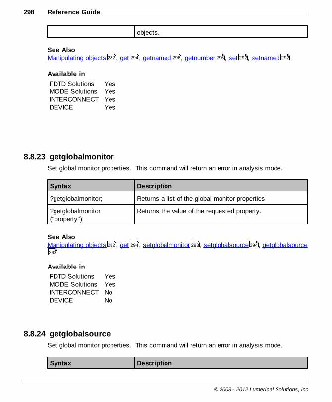
Reference Guide298
© 2003 - 2012 Lumerical Solutions, Inc
objects.
See Also Manipulating objects , get , getnamed , getnumber , set , setnamed
Available in
FDTD SolutionsMODE SolutionsINTERCONNECTDEVICE
YesYesYesYes
8.8.23 getglobalmonitor
Set global monitor properties. This command will return an error in analysis mode.
Syntax Description
?getglobalmonitor; Returns a list of the global monitor properties
?getglobalmonitor("property");
Returns the value of the requested property.
See Also Manipulating objects , get , setglobalmonitor , setglobalsource , getglobalsource
Available in
FDTD SolutionsMODE SolutionsINTERCONNECTDEVICE
YesYesNoNo
8.8.24 getglobalsource
Set global monitor properties. This command will return an error in analysis mode.
Syntax Description
282 294 296 296 292 292
282 294 293 294
298
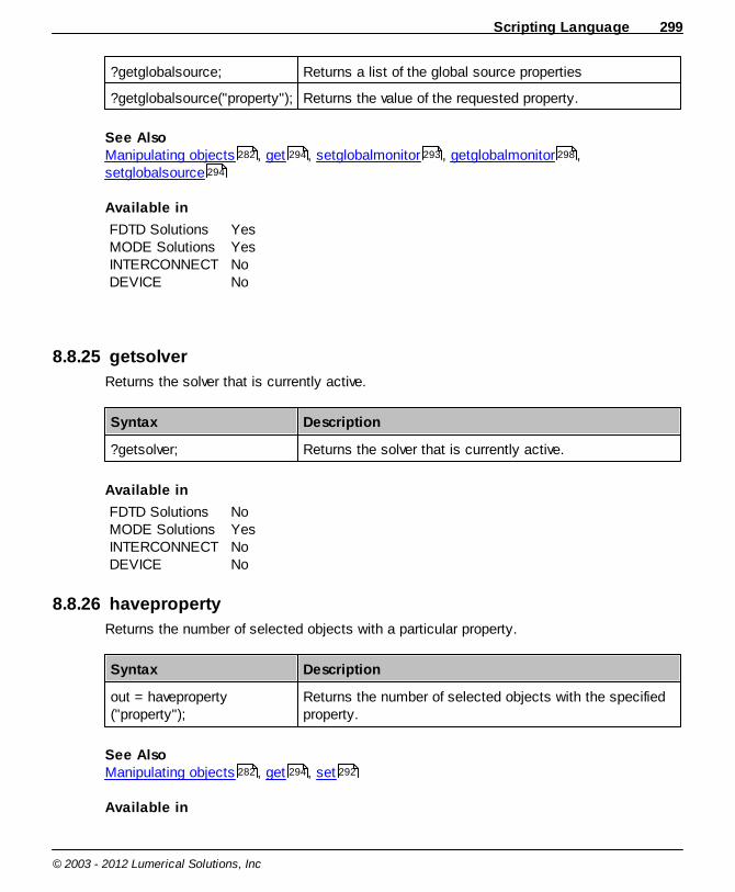
Scripting Language 299
© 2003 - 2012 Lumerical Solutions, Inc
?getglobalsource; Returns a list of the global source properties
?getglobalsource("property"); Returns the value of the requested property.
See Also Manipulating objects , get , setglobalmonitor , getglobalmonitor ,setglobalsource
Available in
FDTD SolutionsMODE SolutionsINTERCONNECTDEVICE
YesYesNoNo
8.8.25 getsolver
Returns the solver that is currently active.
Syntax Description
?getsolver; Returns the solver that is currently active.
Available in
FDTD SolutionsMODE SolutionsINTERCONNECTDEVICE
NoYesNoNo
8.8.26 haveproperty
Returns the number of selected objects with a particular property.
Syntax Description
out = haveproperty("property");
Returns the number of selected objects with the specifiedproperty.
See Also Manipulating objects , get , set
Available in
282 294 293 298
294
282 294 292
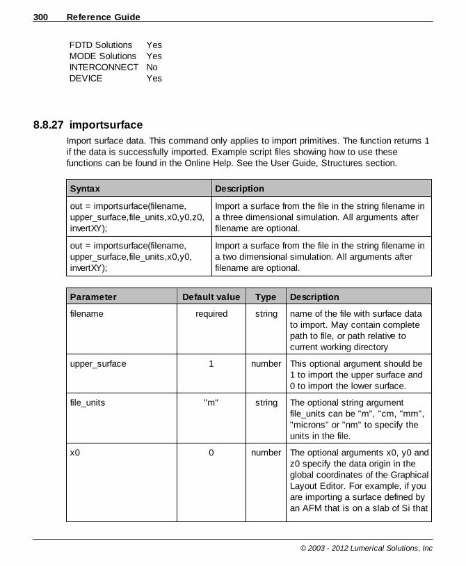
Reference Guide300
© 2003 - 2012 Lumerical Solutions, Inc
FDTD SolutionsMODE SolutionsINTERCONNECTDEVICE
YesYesNoYes
8.8.27 importsurface
Import surface data. This command only applies to import primitives. The function returns 1if the data is successfully imported. Example script files showing how to use thesefunctions can be found in the Online Help. See the User Guide, Structures section.
Syntax Description
out = importsurface(filename,upper_surface,file_units,x0,y0,z0,invertXY);
Import a surface from the file in the string filename ina three dimensional simulation. All arguments afterfilename are optional.
out = importsurface(filename,upper_surface,file_units,x0,y0,invertXY);
Import a surface from the file in the string filename ina two dimensional simulation. All arguments afterfilename are optional.
Parameter Default value Type Description
filename required string name of the file with surface datato import. May contain completepath to file, or path relative tocurrent working directory
upper_surface 1 number This optional argument should be1 to import the upper surface and0 to import the lower surface.
file_units "m" string The optional string argumentfile_units can be "m", "cm, "mm","microns" or "nm" to specify theunits in the file.
x0 0 number The optional arguments x0, y0 andz0 specify the data origin in theglobal coordinates of the GraphicalLayout Editor. For example, if youare importing a surface defined byan AFM that is on a slab of Si that

Scripting Language 301
© 2003 - 2012 Lumerical Solutions, Inc
ranges from 0 to 2 microns, youshould set z0 to 2 microns.
y0 0 number
z0 0 number
invertXY 0 number The optional argument invertXYcan be used to reverse how the xand y axes are read from the file.
See Also Manipulating objects , importsurface2
Available in
FDTD SolutionsMODE SolutionsINTERCONNECTDEVICE
YesYesNoNo
8.8.28 importsurface2
Import surface data from script variables. This command only applies to import primitives.The function returns 1 if the data is successfully imported. Example script files showinghow to use these functions can be found in the Online Help. See the User Guide,Structures section.
Syntax Description
out = importsurface2(Z,x,y,upper_surface);
Import a surface from the variables Z, x and y in threedimensional simulations. The upper_surfaceargument is optional.
out = importsurface2(Y,x,upper_surface);
Import a surface from the variables Y and x in twodimensional simulations. The upper_surfaceargument is optional.
Parameter Default value Type Description
Z required matrix The two dimensional matrix thatdefines the surface.
282 301

Reference Guide302
© 2003 - 2012 Lumerical Solutions, Inc
x required matrix If Z is an NxM matrix, then xshould have dimension Nx1. Fortwo dimensional simulation, if Y isan Nx1 matrix then x should havedimension Nx1.
y required matrix If Z is an NxM matrix, then yshould have dimension Mx1.
upper_surface 1 number This optional argument should be1 to import the upper surface and0 to import the lower surface.
Y required matrix This argument should be an Nx1matrix that defines the surface fortwo dimensional simulations.
See Also Manipulating objects , importsurface
Available in
FDTD SolutionsMODE SolutionsINTERCONNECTDEVICE
YesYesNoNo
8.8.29 importnk
Import the refractive index (n and k) over an entire volume or surface from a file. Thiscommand only applies to import primitives. The function returns 1 if the data is successfullyimported. Example script files showing how to use these functions can be found in theOnline Help. See the User Guide, Structures section.
Note: Uniform gridThe n,k import only works for uniform x,y,z grids. If grid values are non-uniform,interpolated values are incorrect.
Syntax Description
out = importnk(filename,file_units,x0,y0,z0,reverse_index_order);
Import n (and k) data from filename in threedimensional simulations. All arguments after thefilename are optional.
282 300
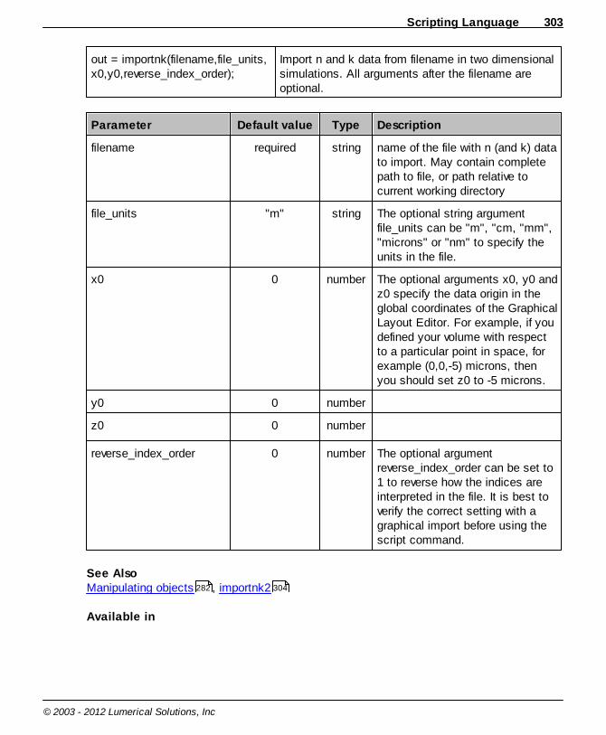
Scripting Language 303
© 2003 - 2012 Lumerical Solutions, Inc
out = importnk(filename,file_units,x0,y0,reverse_index_order);
Import n and k data from filename in two dimensionalsimulations. All arguments after the filename areoptional.
Parameter Default value Type Description
filename required string name of the file with n (and k) datato import. May contain completepath to file, or path relative tocurrent working directory
file_units "m" string The optional string argumentfile_units can be "m", "cm, "mm","microns" or "nm" to specify theunits in the file.
x0 0 number The optional arguments x0, y0 andz0 specify the data origin in theglobal coordinates of the GraphicalLayout Editor. For example, if youdefined your volume with respectto a particular point in space, forexample (0,0,-5) microns, thenyou should set z0 to -5 microns.
y0 0 number
z0 0 number
reverse_index_order 0 number The optional argument reverse_index_order can be set to1 to reverse how the indices areinterpreted in the file. It is best toverify the correct setting with agraphical import before using thescript command.
See Also Manipulating objects , importnk2
Available in
282 304
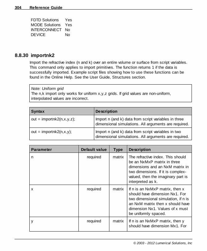
Reference Guide304
© 2003 - 2012 Lumerical Solutions, Inc
FDTD SolutionsMODE SolutionsINTERCONNECTDEVICE
YesYesNoNo
8.8.30 importnk2
Import the refractive index (n and k) over an entire volume or surface from script variables.This command only applies to import primitives. The function returns 1 if the data issuccessfully imported. Example script files showing how to use these functions can befound in the Online Help. See the User Guide, Structures section.
Note: Uniform gridThe n,k import only works for uniform x,y,z grids. If grid values are non-uniform,interpolated values are incorrect.
Syntax Description
out = importnk2(n,x,y,z); Import n (and k) data from script variables in threedimensional simulations. All arguments are required.
out = importnk2(n,x,y); Import n (and k) data from script variables in twodimensional simulations. All arguments are required.
Parameter Default value Type Description
n required matrix The refractive index. This shouldbe an NxMxP matrix in threedimensions and an NxM matrix intwo dimensions. If it is complex-valued, then the imaginary part isinterpreted as k.
x required matrix If n is an NxMxP matrix, then xshould have dimension Nx1. Fortwo dimensional simulation, if n isan NxM matrix then x should havedimension Nx1. Values of x mustbe uniformly spaced.
y required matrix If n is an NxMxP matrix, then yshould have dimension Mx1. For
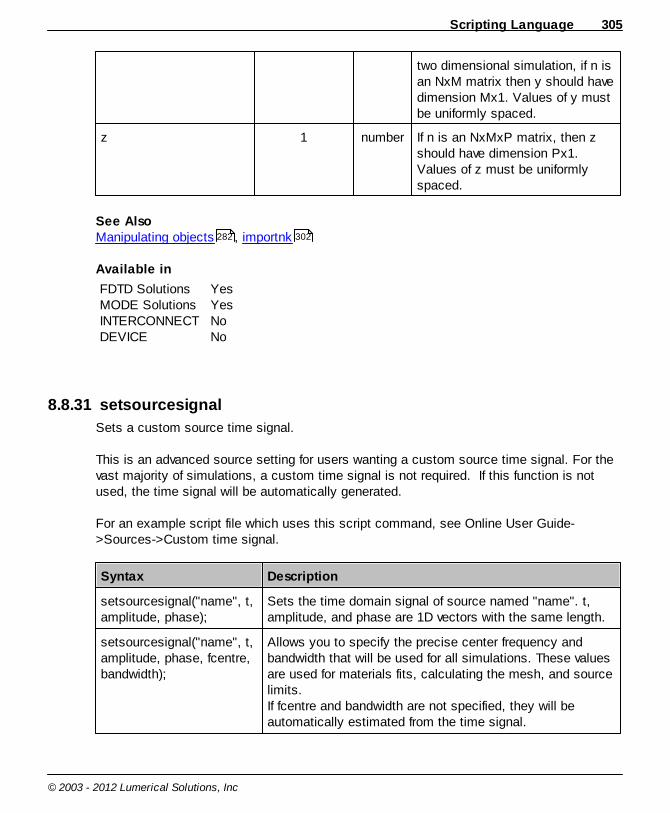
Scripting Language 305
© 2003 - 2012 Lumerical Solutions, Inc
two dimensional simulation, if n isan NxM matrix then y should havedimension Mx1. Values of y mustbe uniformly spaced.
z 1 number If n is an NxMxP matrix, then zshould have dimension Px1.Values of z must be uniformlyspaced.
See Also Manipulating objects , importnk
Available in
FDTD SolutionsMODE SolutionsINTERCONNECTDEVICE
YesYesNoNo
8.8.31 setsourcesignal
Sets a custom source time signal.
This is an advanced source setting for users wanting a custom source time signal. For thevast majority of simulations, a custom time signal is not required. If this function is notused, the time signal will be automatically generated.
For an example script file which uses this script command, see Online User Guide->Sources->Custom time signal.
Syntax Description
setsourcesignal("name", t,amplitude, phase);
Sets the time domain signal of source named "name". t,amplitude, and phase are 1D vectors with the same length.
setsourcesignal("name", t,amplitude, phase, fcentre,bandwidth);
Allows you to specify the precise center frequency andbandwidth that will be used for all simulations. These valuesare used for materials fits, calculating the mesh, and sourcelimits.If fcentre and bandwidth are not specified, they will beautomatically estimated from the time signal.
282 302
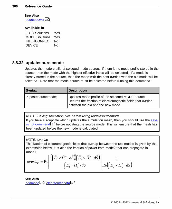
Reference Guide306
© 2003 - 2012 Lumerical Solutions, Inc
See Also sourcepower
Available in
FDTD SolutionsMODE SolutionsINTERCONNECTDEVICE
YesYesNoNo
8.8.32 updatesourcemode
Updates the mode profile of selected mode source. If there is no mode profile stored in thesource, then the mode with the highest effective index will be selected. If a mode isalready stored in the source, then the mode with the best overlap with the old mode will beselected. Note that the mode source must be selected before running this command.
Syntax Description
?updatesourcemode; Updates mode profile of the selected MODE source. Returns the fraction of electromagnetic fields that overlapbetween the old and the new mode
NOTE: Saving simulation files before using updatesourcemodeIf you have a script file which updates the simulation mesh, then you should use the savescript command before updating the source mode. This will ensure that the mesh hasbeen updated before the new mode is calculated.
NOTE: overlapThe fraction of electromagnetic fields that overlap between the two modes is given by theexpression below. It is also the fraction of power from mode2 that can propagate inmode1.
SdHESdHE
SdHESdHEoverlap
*22
*11
*12
*21
Re
1Re
See Also addmode , clearsourcedata
329
161
272 307
Scripting Language 307
© 2003 - 2012 Lumerical Solutions, Inc
Available in
FDTD SolutionsMODE SolutionsINTERCONNECTDEVICE
YesYesNoNo
8.8.33 clearsourcedata
Clears source data for an imported source, or the selected mode for a mode source.
Syntax Description
clearsourcedata; Clears source data for the selected source.
ExampleClear source data from an imported source. This will make the file much smaller, whichcan be convenient when emailing simulation files.
select("source3");clearsourcedata;
See Alsoupdatesourcemode , asapimport , asapload , asapexport
Available in
FDTD SolutionsMODE SolutionsINTERCONNECTDEVICE
YesYesNoNo
8.8.34 redraw
Force the graphical viewports of the CAD to update. The viewports update automatically bydefault, so this command is only required after using the redrawoff command.
Syntax Description
redraw; Redraws graphics.This function does not return any data.
306 177 176 176
Reference Guide308
© 2003 - 2012 Lumerical Solutions, Inc
See Also Manipulating objects , redrawon , redrawoff , redrawmode
Available in
FDTD SolutionsMODE SolutionsINTERCONNECTDEVICE
YesYesNoYes
8.8.35 redrawoff
Disable automatic updating of the graphical viewports in the CAD. This can greatlyincrease the speed of scripts that add large numbers of objects.
Syntax Description
redrawoff; Prevents redrawing of graphics.This function does not return any data.
See Also Manipulating objects , redrawon , redraw , redrawmode
Available in
FDTD SolutionsMODE SolutionsINTERCONNECTDEVICE
YesYesNoYes
8.8.36 redrawon
Enable automatic updating of the graphical viewports in the CAD. Automatic updating isthe default behavior, so this command is only required after using the redrawoff command.
Syntax Description
redrawon; Turns redrawing back on.This function does not return any data.
282 308 308 309
282 308 307 309

Scripting Language 309
© 2003 - 2012 Lumerical Solutions, Inc
See Also Manipulating objects , redraw , redrawoff , redrawmode
Available in
FDTD SolutionsMODE SolutionsINTERCONNECTDEVICE
YesYesNoYes
8.8.37 redrawmode
This command can be used to determine the current status of automatic redrawing. It canalso be used to set the current status of automatic redrawing. The graphics will be redrawnafter any script command that may change the properties of a graphical object.
Syntax Description
out = redrawmode; The value of out indicates if automatic redrawing is off or onout=1: automatic redrawing is onout=0: automatic redrawing is off
out = redrawmode(in); Set the automatic redrawing off or on. To turn it on, usein=1. To turn it off, use in=0. The value of out is set afterexecuting the command so that out=in once this commandhas been executed.
See Also Manipulating objects , redraw , redrawoff
Available in
FDTD SolutionsMODE SolutionsINTERCONNECTDEVICE
YesYesNoYes
282 307 308 309
282 307 308

Reference Guide310
© 2003 - 2012 Lumerical Solutions, Inc
8.8.38 setview
This command allows the viewing properties of the Layout Editor to be modified.
Syntax Description
outstring = setview; Returns a list of the view properties that can be set. Thecommand?setview;
will returnextent, zoom, theta, phi
setview("property"); Sets the default value for any of the view properties. Forexample,setview("extent");
is the same as pressing the graphical extent button.
setview("property",value); Sets the values to of any property for viewing.
The following table describes the properties that can be set
Property Description
extent Control the view extent. In this case, value should be a2x1, 4x1 or 6x1 matrix representing the view range min x,max x, min y, max y, min z and max z respectively.
zoom Controls the relative zoom of the perspective viewcompared to the default level. To zoom in by a factor of 2 inthe perspective view, use setview("zoom",2);
theta Controls the polar angle of the perspective view, indegrees.
phi Controls the azimuthal angle of the perspective view, indegrees.
See Also Manipulating objects , getview , orbit , redraw
Available in
FDTD SolutionsMODE SolutionsINTERCONNECTDEVICE
YesYesNoYes
282 311 311 307
Scripting Language 311
© 2003 - 2012 Lumerical Solutions, Inc
8.8.39 getview
This command allows the viewing properties of the Layout Editor to be retrieved.
Syntax Description
outstring = getview; Returns a list of the view properties that can be set. Thecommand?getview;
will returnextent, zoom, theta, phi
out = getview("property"); Returns the current value of any of the view properties. Forexample,zoom_level = getview("zoom");
will return the current zoom setting of the perspective viewrelative to the default level.
The properties that can be obtained with getview are described in setview .
See Also Manipulating objects , setview , orbit , redraw
Available in
FDTD SolutionsMODE SolutionsINTERCONNECTDEVICE
YesYesNoYes
8.8.40 orbit
This command performs an elliptical viewing orbit of the structure in the perspective view.Note that the commands setview , getview and redraw make it possible to createany type of orbit you would like in your own script file.
Syntax Description
orbit; Performs an orbit of the current perspective view.
orbit(zoom_factor); Performs an orbit with the specified minimum zoom
310
282 310 311 307
310 311 307
Reference Guide312
© 2003 - 2012 Lumerical Solutions, Inc
factor. By default the zoom factor is 1.5.
orbit(zoom_factor, frame_rate); Performs an orbit with the specified frame ratespecified in frames per second. The default frame rateis 15.
orbit(zoom_factor, frame_rate,"filename");
The orbit will be streamed to the mpeg file filename forlater viewing.
See Also Manipulating objects , setview , getview , framerate
Available in
FDTD SolutionsMODE SolutionsINTERCONNECTDEVICE
YesYesNoYes
8.8.41 framerate
Orbits the perspective view and returns the framerate. This can be useful for estimating yourgraphics performance. If comparing the performance of two computers, be sure to useexactly the same simulation file.
Syntax Description
fr = framerate(num_frames,zoom);
num_frames - Number of frames to drawzoom - Zoom factor used in perspective viewfr - number of frames / wall time required to completeorbit.
See Also Manipulating objects , setview , getview , orbit
Available in
FDTD SolutionsMODE SolutionsINTERCONNECTDEVICE
YesNoNoNo
282 310 311 312
282 310 311 311
Scripting Language 313
© 2003 - 2012 Lumerical Solutions, Inc
8.8.42 undo
Undo the last command that modified any objects, you can undo the last 5 commands.
Syntax Description
undo; Undo last modify object command.This function does not return any data.
See Also Manipulating objects , redo
Available in
FDTD SolutionsMODE SolutionsINTERCONNECTDEVICE
YesYesYesYes
8.8.43 redo
Redo a command after a previous undo.
Syntax Description
redo; Redo command after previous undo.This function does not return any data.
See Also Manipulating objects , undo
Available in
FDTD SolutionsMODE SolutionsINTERCONNECTDEVICE
YesYesYesYes
282 313
282 313
Reference Guide314
© 2003 - 2012 Lumerical Solutions, Inc
8.8.44 addport
Add a port to a compound/script element. (Note that this command does not apply forprimitive elements.)
Syntax Description
addport("element", "port","type", "data");
Adds a new port to the element with the specifiedproperties.Returns the name of the port that is created.
Property Defaultvalue
Type Description
element required string Name of the element to add aport to.
port required string Name of the port to add. Thenamed will be modified if thereis already a port of the samename.
type required string The type of port to add. Theoptions are: Bidirectional,Input, Output, Analyzer Input
data required string The type of data for the port.The options are: Variant,Optical Signal, ElectricalSignal, Digital Signal
Manipulating objects , removeport
Available in
FDTD SolutionsMODE SolutionsINTERCONNECTDEVICE
NoNoYesNo
282 315
Scripting Language 315
© 2003 - 2012 Lumerical Solutions, Inc
8.8.45 removeport
Remove a port from a compound/script element. (Note that this command does not applyfor primitive elements.)
Syntax Description
removeport("element","port");
Removes "port" from "element".Returns 1 if the port is successfully removed, 0 otherwise.
Manipulating objects , addport
Available in
FDTD SolutionsMODE SolutionsINTERCONNECTDEVICE
NoNoYesNo
8.8.46 connect
Connects one element to another via the specified ports.
Syntax Description
connect("element1", "port1","element2", "port2");
Connects "port1" of "element1" to "element2" or "port2".
Manipulating objects , disconnect
Available in
FDTD SolutionsMODE SolutionsINTERCONNECTDEVICE
NoNoYesNo
282 314
282 316
Reference Guide316
© 2003 - 2012 Lumerical Solutions, Inc
8.8.47 disconnect
Disconnect one element to another via the specified ports.
Syntax Description
connect("element1", "port1","element2", "port2");
Deletes the connection between "port1" of "element1" and"port2" of "element2".
Manipulating objects , connect
Available in
FDTD SolutionsMODE SolutionsINTERCONNECTDEVICE
NoNoYesNo
8.9 Running simulationsMoving between tabs
Command Description
switchtolayout Closes the analysis window and allows you tomanipulate simulation objects for a new simulation.
layoutmode Used to determine if the simulation file is open inlayout or in analysis mode.
Running Simulations
Command Description
run Launch the simulation. (Options available)
runparallel Launch the simulation in parallel mode.
addjob Add a simulation to the job queue.
runjobs Run all simulations in the job queue.
clearjobs Remove all simulations from the job queue.
runsweep Runs a parameter sweep or optimization task
282 315
264
264
317
317
318
318
319
319
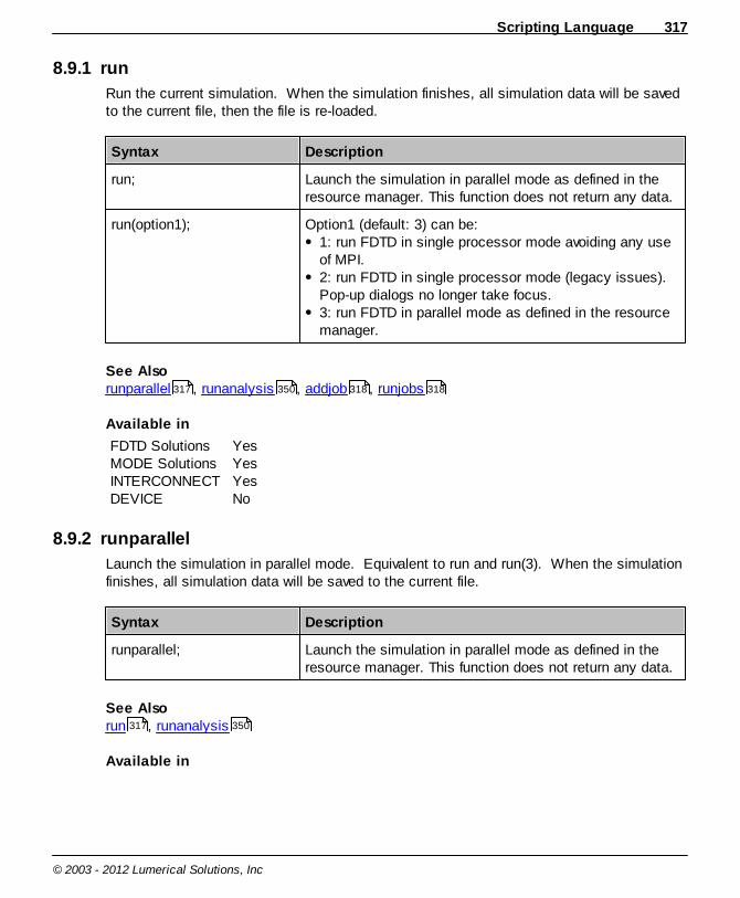
Scripting Language 317
© 2003 - 2012 Lumerical Solutions, Inc
8.9.1 run
Run the current simulation. When the simulation finishes, all simulation data will be savedto the current file, then the file is re-loaded.
Syntax Description
run; Launch the simulation in parallel mode as defined in theresource manager. This function does not return any data.
run(option1); Option1 (default: 3) can be:1: run FDTD in single processor mode avoiding any useof MPI.2: run FDTD in single processor mode (legacy issues).Pop-up dialogs no longer take focus. 3: run FDTD in parallel mode as defined in the resourcemanager.
See Also runparallel , runanalysis , addjob , runjobs
Available in
FDTD SolutionsMODE SolutionsINTERCONNECTDEVICE
YesYesYesNo
8.9.2 runparallel
Launch the simulation in parallel mode. Equivalent to run and run(3). When the simulationfinishes, all simulation data will be saved to the current file.
Syntax Description
runparallel; Launch the simulation in parallel mode as defined in theresource manager. This function does not return any data.
See Also run , runanalysis
Available in
317 350 318 318
317 350
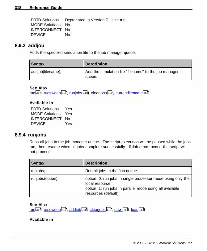
Reference Guide318
© 2003 - 2012 Lumerical Solutions, Inc
FDTD SolutionsMODE SolutionsINTERCONNECTDEVICE
Deprecated in Version 7. Use run.NoNoNo
8.9.3 addjob
Adds the specified simulation file to the job manager queue.
Syntax Description
addjob(filename); Add the simulation file "filename" to the job managerqueue.
See Also run , runsweep , runjobs , clearjobs , currentfilename
Available in
FDTD SolutionsMODE SolutionsINTERCONNECTDEVICE
YesYesNoYes
8.9.4 runjobs
Runs all jobs in the job manager queue. The script execution will be paused while the jobsrun, then resume when all jobs complete successfully. If Job errors occur, the script willnot proceed.
Syntax Description
runjobs; Run all jobs in the Job queue.
runjobs(option); option=0: run jobs in single processor mode using only thelocal resource.option=1: run jobs in parallel mode using all availableresources (default).
See Also run , runsweep , addjob , clearjobs , save , load
Available in
317 319 318 319 167
317 319 318 319 161 161
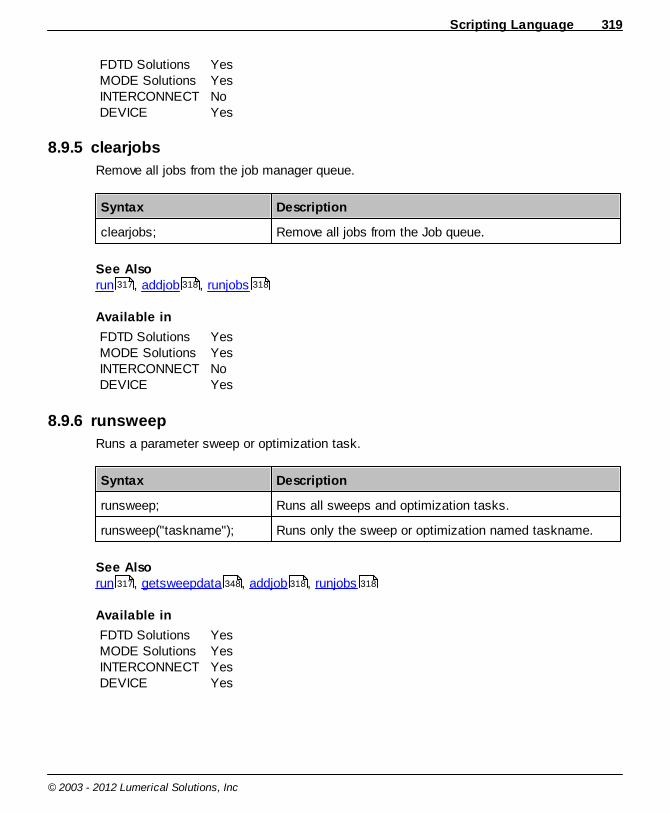
Scripting Language 319
© 2003 - 2012 Lumerical Solutions, Inc
FDTD SolutionsMODE SolutionsINTERCONNECTDEVICE
YesYesNoYes
8.9.5 clearjobs
Remove all jobs from the job manager queue.
Syntax Description
clearjobs; Remove all jobs from the Job queue.
See Also run , addjob , runjobs
Available in
FDTD SolutionsMODE SolutionsINTERCONNECTDEVICE
YesYesNoYes
8.9.6 runsweep
Runs a parameter sweep or optimization task.
Syntax Description
runsweep; Runs all sweeps and optimization tasks.
runsweep("taskname"); Runs only the sweep or optimization named taskname.
See Also run , getsweepdata , addjob , runjobs
Available in
FDTD SolutionsMODE SolutionsINTERCONNECTDEVICE
YesYesYesYes
317 318 318
317 348 318 318
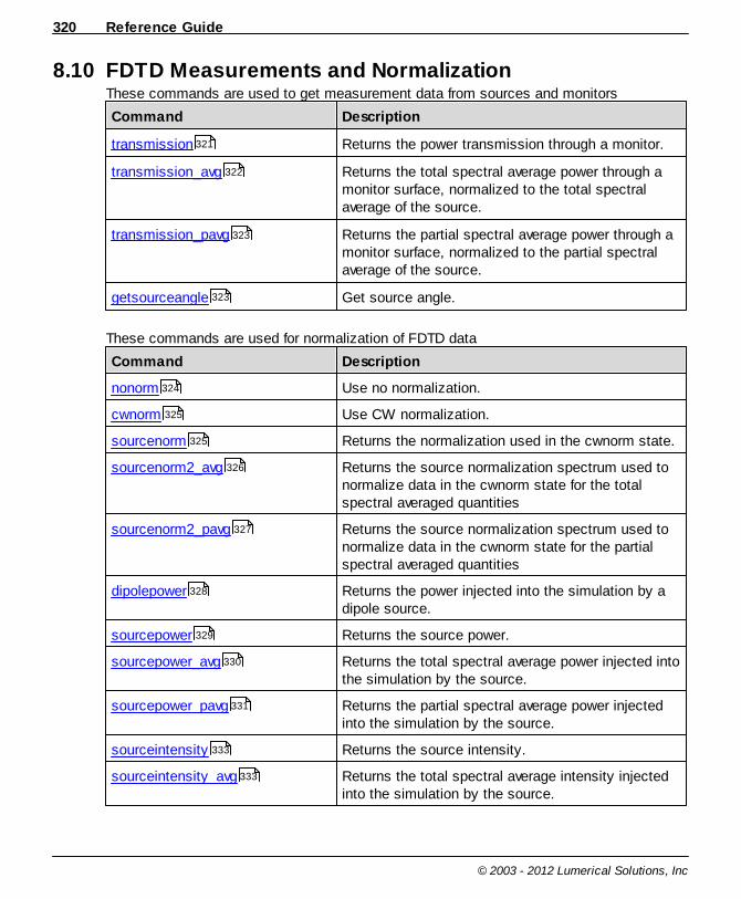
Reference Guide320
© 2003 - 2012 Lumerical Solutions, Inc
8.10 FDTD Measurements and NormalizationThese commands are used to get measurement data from sources and monitors
Command Description
transmission Returns the power transmission through a monitor.
transmission_avg Returns the total spectral average power through amonitor surface, normalized to the total spectralaverage of the source.
transmission_pavg Returns the partial spectral average power through amonitor surface, normalized to the partial spectralaverage of the source.
getsourceangle Get source angle.
These commands are used for normalization of FDTD data
Command Description
nonorm Use no normalization.
cwnorm Use CW normalization.
sourcenorm Returns the normalization used in the cwnorm state.
sourcenorm2_avg Returns the source normalization spectrum used tonormalize data in the cwnorm state for the totalspectral averaged quantities
sourcenorm2_pavg Returns the source normalization spectrum used tonormalize data in the cwnorm state for the partialspectral averaged quantities
dipolepower Returns the power injected into the simulation by adipole source.
sourcepower Returns the source power.
sourcepower_avg Returns the total spectral average power injected intothe simulation by the source.
sourcepower_pavg Returns the partial spectral average power injectedinto the simulation by the source.
sourceintensity Returns the source intensity.
sourceintensity_avg Returns the total spectral average intensity injectedinto the simulation by the source.
321
322
323
323
324
325
325
326
327
328
329
330
331
333
333

Scripting Language 321
© 2003 - 2012 Lumerical Solutions, Inc
sourceintensity_pavg Returns the partial spectral average intensity injectedinto the simulation by the source.
8.10.1 transmission
The transmission function returns the amount of power transmitted through power monitorsand profile monitors, normalized to the source power. A value of 0.5 means that half of theoptical power injected by the source passed through the monitor. Negative values mean thepower is flowing in the negative direction.
The transmission is calculated with the following formula.
rsourcepowe
dSfPrealfT
Monitor)(2
1
)(
where T(f) is the normalized transmission as a function of frequency P(f) is the Poynting vector dS is the surface normal
The normalization state (cwnorm or nonorm) does not affect the result because of thesource power normalization.
Syntax Description
out = transmission( "mname");
Transmission through monitor mname. It must be obviousfrom the shape of the monitor which axis is normal to themonitor surface.
out = transmission( "mname", option);
The additional argument, option, can have a value of 1 or 2.If it is 2, the data is unfolded where possible according tothe symmetry or anti-symmetric boundaries if it comesfrom a monitor that intersect such a boundary at x min, ymin or z min. The default value of option is 2.
See Alsosourcepower , dipolepower , transmission_avg , transmission_pavg
Available in
334
329 328 322 323
Reference Guide322
© 2003 - 2012 Lumerical Solutions, Inc
FDTD SolutionsMODE SolutionsINTERCONNECTDEVICE
YesYesNoNo
8.10.2 transmission_avg
Returns the total spectral average power through a monitor surface, normalized to the totalspectral average of the source. See the Units and normalization - Spectral averagingsection for more information.
avgrsourcepowe
dSPrealT
total
Monitor
avg_
2
1
where Tav g
is the normalized total spectral average transmission
<P> is the total spectral average Poynting vector dS is the surface normal
The normalization state (cwnorm or nonorm) does not affect the result because of thesource power normalization.
Syntax Description
out = transmission_avg( "monitorname");
Returns the total spectral average transmission throughmonitorname. It must be obvious from the shape of themonitor which axis is normal to the monitor surface.
out = transmission_avg( "monitorname", option);
The additional argument, option, can have a value of 1 or 2.If it is 2, the data is unfolded where possible according tothe symmetry or anti-symmetric boundaries if it comesfrom a monitor that intersect such a boundary at x min, ymin or z min. The default value of option is 2.
See Alsosourcepower_avg , transmission , transmission_pavg , Units and Normalization,Spectral averaging
Available in
FDTD SolutionsMODE SolutionsINTERCONNECTDEVICE
YesYesNoNo
330 321 323

Scripting Language 323
© 2003 - 2012 Lumerical Solutions, Inc
8.10.3 transmission_pavg
Returns the partial spectral average power through a monitor surface, normalized to thepartial spectral average of the source. See the Units and normalization - Spectral averagingsection for more information.
)(_
)(2
1
)(fpavgrsourcepowe
dSfPrealfT
partial
Monitor
pavg
where Tpav g
is the normalized partial spectral average transmission
<P> is the partial spectral average Poynting vectordS is the surface normal
The normalization state (cwnorm or nonorm) does not affect the result because of thesource power normalization.
Syntax Description
out = transmission_pavg( "monitorname" );
Returns the partial spectral average transmission throughmonitorname. It must be obvious from the shape of themonitor which axis is normal to the monitor surface.
out = transmission_pavg( "monitorname", option );
The additional argument, option, can have a value of 1 or 2.If it is 2, the data is unfolded where possible according tothe symmetry or anti-symmetric boundaries if it comesfrom a monitor that intersect such a boundary at x min, ymin or z min. The default value of option is 2.
See Alsosourcepower_pavg , transmission , transmission_avg , Units and Normalization,Spectral averaging
Available in
FDTD SolutionsMODE SolutionsINTERCONNECTDEVICE
YesYesNoNo
8.10.4 getsourceangle
Broadband sources inject fields that have a constant in-plane wavevector at all frequencies.This implies injection angle must change as a function of frequency. The in-planewavevector is chosen such that the incidence angle at the center frequency of thesimulation (fSIM) will match the source angle theta (thetaSIM) specified in the source
331 321 322

Reference Guide324
© 2003 - 2012 Lumerical Solutions, Inc
properties. Higher frequencies will be injected at smaller angles, while lower frequencieswill be injected at larger angles. This 'theta vs wavelength' plot in the beam source editwindow shows the same function.
f
faf SIMSIM )sin(
sin)(
Syntax Description
theta = getsourceangle( "sourcename", f);
Returns the source angle theta (degrees) as a function offrequency. f is a vector of frequencies (Hz).
See Alsosourcepower , Online Help-User Guide-Sources-Broadband injection angles
Available in
FDTD SolutionsMODE SolutionsINTERCONNECTDEVICE
YesYesNoNo
8.10.5 nonorm
Do not normalized the data to the source power. The actual field intensities will be used inall calculations. This function controls the checkbox located in Settings - Normalization state.
Syntax Description
nonorm; Use no normalization.This function does not return any data.
See Alsocwnorm , Units and Normalization
Available in
FDTD SolutionsMODE SolutionsINTERCONNECTDEVICE
YesYesNoNo
329
325
Scripting Language 325
© 2003 - 2012 Lumerical Solutions, Inc
8.10.6 cwnorm
Use CW normalization. All simulation data will be normalized to the injected source power. Most users prefer to do their analysis in the CW normalization state, since it removes anyeffect caused by the finite pulse length of the source. It also converts the units of allelectromagnetic fields to be the same as in the time domain.
This function controls the checkbox located in Settings - Normalization state.
Syntax Description
cwnorm; Use CW normalization.This function does not return any data.
See Alsononorm , Units and Normalization
Available in
FDTD SolutionsMODE SolutionsINTERCONNECTDEVICE
YesYesNoNo
8.10.7 sourcenorm
Returns the source normalization spectrum used to normalize data in the cwnorm state forstandard fourier transform quantities. See the Units and normalization chapter for moreinformation.
If the source time signal of the jth source in the simulation is sj(t), and N is the number of
active sources then
sourcesj dtsti
Nsourcenorms )(exp
1)()(
Syntax Description
out = sourcenorm(f); Returns the source normalization used to normalize data inthe cwnorm state at the vector of frequency points f. (f isthe frequency in Hz)
out = sourcenorm(f, name); This function makes it possible to perform thenormalization using the spectrum of one source, ratherthan the sum of all the sources.
324
Reference Guide326
© 2003 - 2012 Lumerical Solutions, Inc
See Alsosourcenorm2_avg , sourcenorm2_pavg , sourcepower , cwnorm , nonorm ,Units and Normalization
Available in
FDTD SolutionsMODE SolutionsINTERCONNECTDEVICE
YesYesNoNo
8.10.8 sourcenorm2_avg
Returns the source normalization spectrum used to normalize data in the cwnorm state forthe total spectral averaged quantities. See the Units and normalization - Spectral averagingsection for more information.
The script function sourcenorm is defined as
sourcesj dtsti
Nsourcenorms )(exp
1)()(
If sourcenorm2_avg is called without any arguments, it returns
')'(_22
dsavgsourcenorm
Syntax Description
out = sourcenorm2_avg; This function returns the source normalization for totalspectral averaged quantities.
out = sourcenorm2_avg( "sourcename");
This function makes it possible to perform thenormalization using the spectrum of one source, ratherthan the sum of all the sources.
See Alsosourcenorm , sourcenorm2_pavg , sourcepower_avg , cwnorm , nonorm ,Units and Normalization, Spectral averaging
Available in
326 327 329 325 324
325 327 330 325 324
Scripting Language 327
© 2003 - 2012 Lumerical Solutions, Inc
FDTD SolutionsMODE SolutionsINTERCONNECTDEVICE
YesYesNoNo
8.10.9 sourcenorm2_pavg
Returns the source normalization spectrum used to normalize data in the cwnorm state forthe partial spectral averaged quantities. See the Units and normalization - Spectralaveraging section for more information.
If the source time signal of the jth source in the simulation is sj(t), and N is the number of
active sources then
sourcesj dtsti
Nsourcenorms )(exp
1)()(
Partial spectral averaging uses a Lorentzian weighting of the following form. Delta is the
FWHM of |h|2.
1')',(
)2/()'(
1
2)',(
2
22
2
dh
hi
If this function is called without any arguments, it returns
')'()',(_222
dshpavgsourcenorm
Syntax Description
out = sourcenorm2_pavg( f,delta);
This function returns the source normalization for partialspectral averaged quantities.
out = sourcenorm2_pavg( f,delta, "sourcename");
This function makes it possible to perform thenormalization using the spectrum of one source, ratherthan the sum of all the sources.
See Alsosourcenorm , sourcenorm2_avg , sourcepower_pavg , cwnorm , nonorm ,325 326 331 325 324
Reference Guide328
© 2003 - 2012 Lumerical Solutions, Inc
Units and Normalization, Spectral averaging
Available in
FDTD SolutionsMODE SolutionsINTERCONNECTDEVICE
YesYesNoNo
8.10.10 dipolepower
Returns the power injected into the simulation region by a dipole source. In 3D simulations,
the units will be in Watts if cw norm is used, and Watts/Hertz2 if no norm is used.
The dipolepower script command returns the power that was injected into the simulationregion, and is equivalent to measuring the power transmitted out of a small box surroundingthe dipole. In contrast, sourcepower will return the power that an ideal dipole wouldradiate in a homogeneous material. dipolepower and sourcepower are equivalent for dipolesin a homogeneous medium.
Advanced notes:There can be some numerical errors in this calculation that become significant whensmall mesh sizes are used. If the mesh step is the order of, or smaller than, /500, itmay be necessary to measure this quantity using a small box of power monitorssurrounding the dipole.If the dipole is injected into a dispersive medium with a non-zero imaginary part of therefractive index, then the results of this function are not reliable.
Please contact [email protected] for more assistance if you are using a dipole indispersive medium, or in a fine mesh region, and would like to calculate the total poweremitted by the dipole.
Syntax Description
out = dipolepower(f); Returns the amount of power radiated by the dipole source,at frequency points f. (f in Hz)
out = dipolepower(f, name); This option allows you to obtain the power radiated by asingle dipole, rather than the sum of all dipoles. Thisoption is only needed for simulations with multiple dipoles.
See Alsosourcenorm , sourcepower , sourcepower_avg , sourcepower_pavg ,transmission , cwnorm , nonorm , Units and Normalization
Available in
329
325 329 330 331
321 325 324
Scripting Language 329
© 2003 - 2012 Lumerical Solutions, Inc
FDTD SolutionsMODE SolutionsINTERCONNECTDEVICE
YesYesNoNo
8.10.11 sourcepower
Returns the power that an ideal source would inject into homogeneous material. In 3D
simulations, the units will be in Watts if CW norm is used, and Watts/Hertz2 if no norm isused. For beam sources (Gaussian, plane wave) and mode sources, the sourcepower is
determined from the equation below. Note that
SourcefP )( is the Poynting vector
determined by the fields that an ideal source would have in a homogeneous material, andthe integral is computed over the injection region of the source.
dSfPrealfrsourcepowe Sourcenonorm )(
2
1)(
2
)(2
1
)(sourcenorm
dSfPrealfrsourcepowe
Source
cwnorm
For simulations using beam sources, sourcepower gives the amount of power injected intothe simulation. The only exception is if the simulation is setup such that there is radiationwhich travels through the injection plane of the source in the source injection direction (pinkarrow). In such cases, the actual amount of power injected by the source will not be givenby sourcepower. In almost all cases, this means your simulation is not setup properly.
For point sources (dipole), the sourcepower script function returns the power an ideal dipolesource will radiate in a homogeneous medium. This quantity can be calculated analytically(see Dipoles - Radiated Power page in the User Guide). The actual radiated power is NOTgiven by the sourcepower function. The actual radiated power is highly dependant on thesurrounding materials, since the reflections from the structures will interfere with the fieldsfrom the dipole, changing the actual radiated power. To get the actual radiated power, seethe dipolepower script function. For additional information, see the Dipoles - RadiatedPower page in the User Guide.
Syntax Description
out = sourcepower(f); Returns the source power used to normalize transmission
328
Reference Guide330
© 2003 - 2012 Lumerical Solutions, Inc
calculations at the vector of frequency points f. (f is thefrequency in Hz)
out = sourcepower(f,option);
The additional argument, option, can have a value of 1 or 2.If it is 2, the data is unfolded where possible according tothe symmetry or anti-symmetric boundaries if it comesfrom a monitor that intersect such a boundary at x min, ymin or z min. The default value of option is 2.
out = sourcepower(f, option,name);
This option allows you to obtain the spectrum of onesource, rather than the sum of all sources. This option isonly needed for simulations with multiple sources.
See Alsosourcenorm , sourcepower_avg , sourcepower_pavg , dipolepower , transmission
, sourceintensity , cwnorm , nonorm , Units and Normalization
Available in
FDTD SolutionsMODE SolutionsINTERCONNECTDEVICE
YesYesNoNo
8.10.12 sourcepower_avg
Returns the total spectral average power injected into the simulation by the source. See theUnits and normalization - Spectral averaging section for more information.
This script function calculates the following quantities, depending on whether thenormalization state is cwnorm or nonorm:
0
)(_ drsourcepoweavgrsourcepowe nonormnonorm
0
2
0
2
)(
)()(
)(_
ds
drsourcepowes
favgrsourcepowecwnorm
cwnorm
where sourcepower is the quantity returned by the sourcepower script function, s(w) isreturned by sourcenorm, and =2 f. Typically, this function should be used in the cwnormstate. Also see the sourcenorm2_pavg script function.
325 330 331 328
321 333 325 324
Scripting Language 331
© 2003 - 2012 Lumerical Solutions, Inc
Syntax Description
out = sourcepower_avg; Returns the spectrally averaged source power as definedabove.
out = sourcepower_avg(option);
The additional argument, option, can have a value of 1 or 2.If it is 2, the data is unfolded where possible according tothe symmetry or anti-symmetric boundaries if it comesfrom a monitor that intersect such a boundary at x min, ymin or z min. The default value of option is 2.
out = sourcepower_avg(option, "sourcename");
This option allows you to obtain the spectrum of onesource, rather than the sum of all sources. This option isonly needed for simulations with multiple sources.
See Alsosourcenorm2_avg , sourcepower , sourcepower_pavg , transmission_avg ,sourceintensity_avg , cwnorm , nonorm , Units and Normalization, Spectralaveraging
Available in
FDTD SolutionsMODE SolutionsINTERCONNECTDEVICE
YesYesNoNo
8.10.13 sourcepower_pavg
Returns the partial spectral average power injected into the simulation by the source. Seethe Units and normalization - Spectral averaging section for more information.
Partial spectral averaging uses a Lorentzian weighting of the form
1')',(
)2/()'(
1
2)',(
2
22
2
dh
hi
This script function calculates the following quantities, depending on whether thenormalization state is cwnorm or nonorm:
drsourcepowehfpavgrsourcepowe nonormnonorm )()',()(_2
326 329 331 322
333 325 324
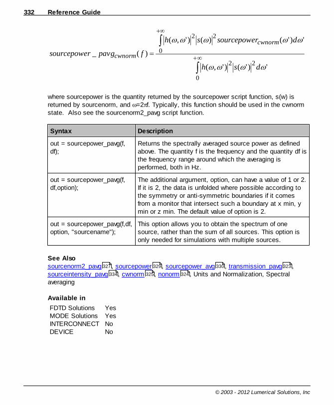
Reference Guide332
© 2003 - 2012 Lumerical Solutions, Inc
0
22
0
22
')'()',(
')'()()',(
)(_
dsh
drsourcepowesh
fpavgrsourcepowe
cwnorm
cwnorm
where sourcepower is the quantity returned by the sourcepower script function, s(w) isreturned by sourcenorm, and =2 f. Typically, this function should be used in the cwnormstate. Also see the sourcenorm2_pavg script function.
Syntax Description
out = sourcepower_pavg(f,df);
Returns the spectrally averaged source power as definedabove. The quantity f is the frequency and the quantity df isthe frequency range around which the averaging isperformed, both in Hz.
out = sourcepower_pavg(f,df,option);
The additional argument, option, can have a value of 1 or 2.If it is 2, the data is unfolded where possible according tothe symmetry or anti-symmetric boundaries if it comesfrom a monitor that intersect such a boundary at x min, ymin or z min. The default value of option is 2.
out = sourcepower_pavg(f,df,option, "sourcename");
This option allows you to obtain the spectrum of onesource, rather than the sum of all sources. This option isonly needed for simulations with multiple sources.
See Alsosourcenorm2_pavg , sourcepower , sourcepower_avg , transmission_pavg ,sourceintensity_pavg , cwnorm , nonorm , Units and Normalization, Spectralaveraging
Available in
FDTD SolutionsMODE SolutionsINTERCONNECTDEVICE
YesYesNoNo
327 329 330 323
334 325 324

Scripting Language 333
© 2003 - 2012 Lumerical Solutions, Inc
8.10.14 sourceintensity
Sourceintensity returns the source power divided by the area of the source. In 3D
simulations, the units will be in Watts/m2 if CW norm is used, and Watts/m2/Hertz2 if Nonorm is used. This function is often used when normalizing power measurements fromsimulations with a TFSF source.
Syntax Description
out = sourceintensity(f); Returns the source intensity at the vector of frequencypoints f (f is the frequency in Hz).
out = sourceintensity(f,option);
The additional argument, option, can have a value of 1 or 2.If it is 2, the data is unfolded where possible according tothe symmetry or anti-symmetric boundaries if it comesfrom a monitor that intersect such a boundary at x min, ymin or z min. The default value of option is 2.
out = sourceintensity(f,option, name);
This function makes it possible to perform thenormalization using the spectrum of one source, ratherthan the sum of all the sources.
See Alsosourcenorm , sourcepower , sourceintensity_avg , sourceintensity_pavg ,dipolepower , transmission , cwnorm , nonorm , Units and Normalization
Available in
FDTD SolutionsMODE SolutionsINTERCONNECTDEVICE
YesYesNoNo
8.10.15 sourceintensity_avg
Returns the total spectral average intensity injected into the simulation by the source. Theaverage intensity is equal to the average power divided by the source area. See the sourcepower_pavg command and the Units and normalization - Spectral averagingsection for more information.
Syntax Description
out = sourceintensity_avg; Returns the spectrally averaged source intensity as definedabove.
out = sourceintensity_avg The additional argument, option, can have a value of 1 or 2.
325 329 333 334
328 321 325 324 37
331
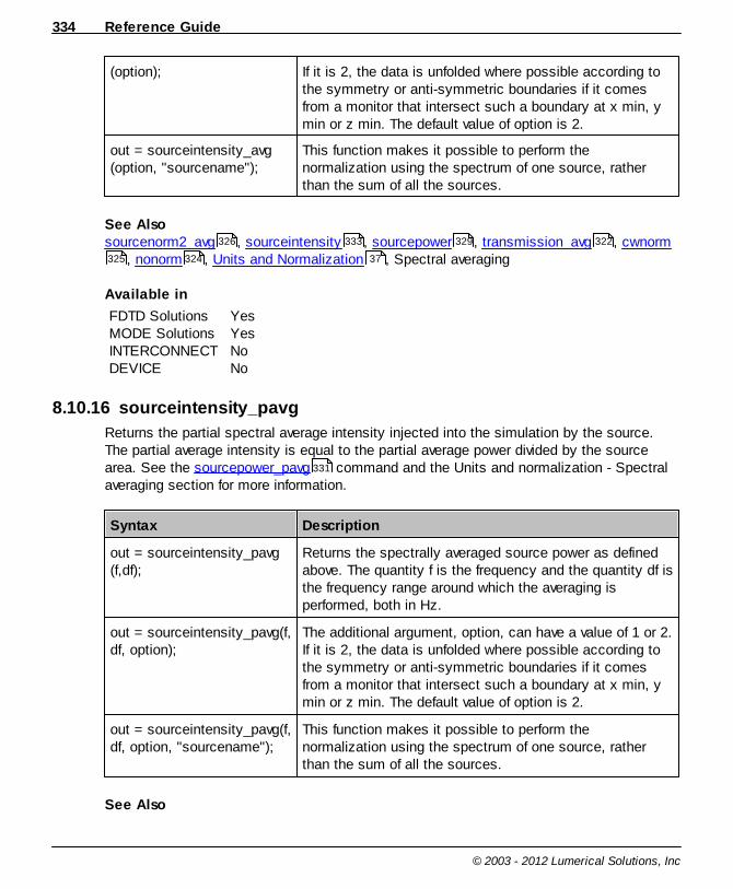
Reference Guide334
© 2003 - 2012 Lumerical Solutions, Inc
(option); If it is 2, the data is unfolded where possible according tothe symmetry or anti-symmetric boundaries if it comesfrom a monitor that intersect such a boundary at x min, ymin or z min. The default value of option is 2.
out = sourceintensity_avg(option, "sourcename");
This function makes it possible to perform thenormalization using the spectrum of one source, ratherthan the sum of all the sources.
See Alsosourcenorm2_avg , sourceintensity , sourcepower , transmission_avg , cwnorm
, nonorm , Units and Normalization , Spectral averaging
Available in
FDTD SolutionsMODE SolutionsINTERCONNECTDEVICE
YesYesNoNo
8.10.16 sourceintensity_pavg
Returns the partial spectral average intensity injected into the simulation by the source.The partial average intensity is equal to the partial average power divided by the sourcearea. See the sourcepower_pavg command and the Units and normalization - Spectralaveraging section for more information.
Syntax Description
out = sourceintensity_pavg(f,df);
Returns the spectrally averaged source power as definedabove. The quantity f is the frequency and the quantity df isthe frequency range around which the averaging isperformed, both in Hz.
out = sourceintensity_pavg(f,df, option);
The additional argument, option, can have a value of 1 or 2.If it is 2, the data is unfolded where possible according tothe symmetry or anti-symmetric boundaries if it comesfrom a monitor that intersect such a boundary at x min, ymin or z min. The default value of option is 2.
out = sourceintensity_pavg(f,df, option, "sourcename");
This function makes it possible to perform thenormalization using the spectrum of one source, ratherthan the sum of all the sources.
See Also
326 333 329 322
325 324 37
331
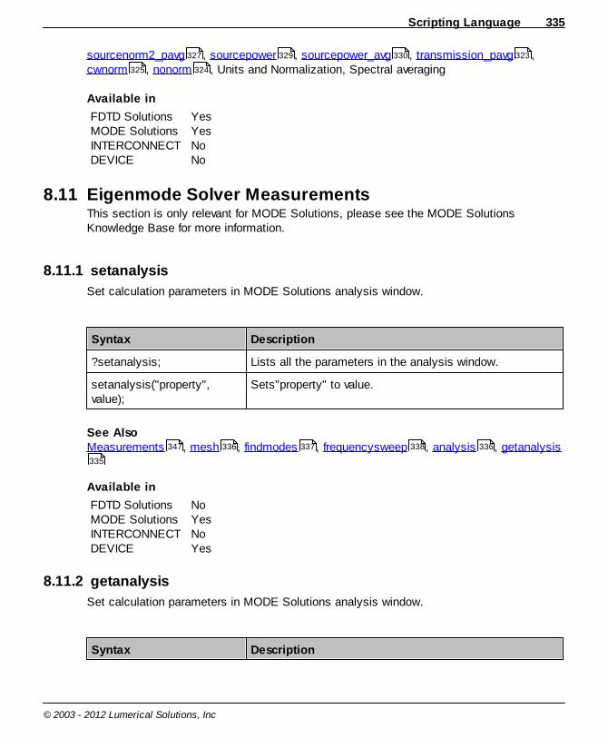
Scripting Language 335
© 2003 - 2012 Lumerical Solutions, Inc
sourcenorm2_pavg , sourcepower , sourcepower_avg , transmission_pavg ,cwnorm , nonorm , Units and Normalization, Spectral averaging
Available in
FDTD SolutionsMODE SolutionsINTERCONNECTDEVICE
YesYesNoNo
8.11 Eigenmode Solver MeasurementsThis section is only relevant for MODE Solutions, please see the MODE SolutionsKnowledge Base for more information.
8.11.1 setanalysis
Set calculation parameters in MODE Solutions analysis window.
Syntax Description
?setanalysis; Lists all the parameters in the analysis window.
setanalysis("property",value);
Sets"property" to value.
See AlsoMeasurements , mesh , findmodes , frequencysweep , analysis , getanalysis
Available in
FDTD SolutionsMODE SolutionsINTERCONNECTDEVICE
NoYesNoYes
8.11.2 getanalysis
Set calculation parameters in MODE Solutions analysis window.
Syntax Description
327 329 330 323
325 324
347 336 337 338 336
335
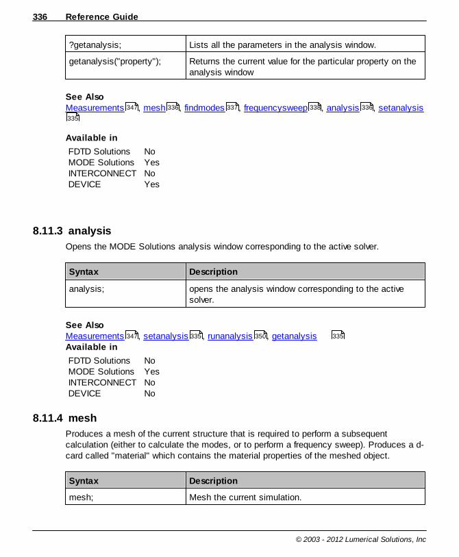
Reference Guide336
© 2003 - 2012 Lumerical Solutions, Inc
?getanalysis; Lists all the parameters in the analysis window.
getanalysis("property"); Returns the current value for the particular property on theanalysis window
See AlsoMeasurements , mesh , findmodes , frequencysweep , analysis , setanalysis
Available in
FDTD SolutionsMODE SolutionsINTERCONNECTDEVICE
NoYesNoYes
8.11.3 analysis
Opens the MODE Solutions analysis window corresponding to the active solver.
Syntax Description
analysis; opens the analysis window corresponding to the activesolver.
See AlsoMeasurements , setanalysis , runanalysis , getanalysis Available in
FDTD SolutionsMODE SolutionsINTERCONNECTDEVICE
NoYesNoNo
8.11.4 mesh
Produces a mesh of the current structure that is required to perform a subsequentcalculation (either to calculate the modes, or to perform a frequency sweep). Produces a d-card called "material" which contains the material properties of the meshed object.
Syntax Description
mesh; Mesh the current simulation.
347 336 337 338 336
335
347 335 350 335
Scripting Language 337
© 2003 - 2012 Lumerical Solutions, Inc
See Alsosetanalysis , mesh , findmodes
Available in
FDTD SolutionsMODE SolutionsINTERCONNECTDEVICE
NoYesNoNo
8.11.5 findmodes
Calculates the modes supported by the structure using the current calculation settings.This function is the script equivalent to the calculate modes button. Each mode will besaved as a D-CARD named "modeX", where X is the xth mode found. The D-CARD savesdata such as effective index and mode profile.
Syntax Description
n=findmodes; n will be equal to the number of modes found.
See Alsosetanalysis , mesh , selectmode , frequencysweep , coupling , overlap ,bestoverlap , propagate
Available in
FDTD SolutionsMODE SolutionsINTERCONNECTDEVICE
NoYesNoNo
8.11.6 selectmode
All modes found in a simulation are numbered based on their effective index. They aredisplayed in the mode table of the Analysis tab. The selectmode command will select theNth mode in the mode table.
Syntax Description
selectmode(N); where N is the number of the desired mode.
selectmode(name); where name is a string containing the name of a mode.
335 336 337
335 336 337 338 338 339
340 341
Reference Guide338
© 2003 - 2012 Lumerical Solutions, Inc
Modes are named mode1, mode2, ..modeN. This form ofthe command is compatible with the bestoverlapfunction
See Also setanalysis , mesh , findmodes , frequencysweep
Available in
FDTD SolutionsMODE SolutionsINTERCONNECTDEVICE
NoYesNoNo
8.11.7 frequencysweep
Performs a frequency sweep using the current settings within the frequency analysis tab.Produces a D-CARD called "frequencysweep" that contains dispersion, effective index, andother data for as a function of frequency.
Syntax Description
frequencysweep; Perform a frequency sweep with the current settings.This function does not return any data.
See Alsosetanalysis , mesh , findmodes , selectmode
Available in
FDTD SolutionsMODE SolutionsINTERCONNECTDEVICE
NoYesNoNo
8.11.8 coupling
The coupling function calculates the complex coupling coefficient between two modes. Thepower coupling can be calculated with the overlap function, or by the following formula.
2aingPowerCoupl
Here 'a' is the ratio of the basis state coefficients. The full formula for a can be found in thefollowing reference:
340
335 336 337 338
335 336 337 337

Scripting Language 339
© 2003 - 2012 Lumerical Solutions, Inc
Allan W. Snyder and John D. Love, Optical Waveguide Theory. Chapman & Hall, London,England, 1983.
See the overlap function for more details about overlap and coupling calculations.
Only available in MODE Solutions.
Syntax Description
out = coupling(mode2,mode1);
mode2, mode1: the mode namesout: the coupling coefficient
out = coupling(mode2,mode1, x, y);
Mode alignment can be adjusted before coupling iscalculated.
x offsety offset
See Alsocopydcard , findmodes , coupling , overlap , bestoverlap , propagate
Available in
FDTD SolutionsMODE SolutionsINTERCONNECTDEVICE
NoYesNoNo
8.11.9 overlap
Calculates the overlap and power coupling between two modes.
Overlap: Measures the fraction of electromagnetic fields that overlap between the twomodes. This is also the fraction of power from mode2 that can propagate in mode1.
SdHESdHE
SdHESdHEoverlap
*22
*11
*12
*21
Re
1Re
Power Coupling: Measures the amount of power that can couple from mode2 into aforward propagating wave with the mode profile of mode1. The remaining power that canpropagate in this mode will couple into the backwards propagating mode. Therefore, thepower coupling is always less than or equal to the overlap. If the two modes have the sameeffective index, then the power coupling will be equal to the overlap.
A dielectric interface is a simple example. The modes on each side of the interface will
351 337 338 339 340 341
Reference Guide340
© 2003 - 2012 Lumerical Solutions, Inc
have an overlap of 1, but the power coupling will be less than one. This is due to reflectionscaused by the index change at the interface.
These calculations are based on the methods described in Snyder and Love "OpticalWaveguide Theory", Chapman & Hall, London, England, 1983.
Syntax Description
out = overlap(mode2,mode1);
mode2, mode1: the mode namesout(1): the mode overlapout(2): the mode power coupling
out = overlap(mode2,mode1, x, y,z);
Mode alignment can be adjusted before overlap iscalculated.
x offsety offsetz offset
The offset is applied to the second mode listed.
See Alsocopydcard , findmodes , coupling , bestoverlap , propagate
Available in
FDTD SolutionsMODE SolutionsINTERCONNECTDEVICE
NoYesNoNo
8.11.10 bestoverlap
Finds the best overlap between the D-CARD called "test_mode" and the currentlycalculated modes. It returns the name of the mode with the best overlap. This function ismainly used for tracking the desired mode during parameter sweeps.
See the overlap function for more details about overlap and coupling calculations.
Syntax Description
out = bestoverlap("test_mode");
Calculates the best overlap.out: a string containing the name of the mode with thebest overlaptest_mode: a string containing the name of a D-CARD
351 337 338 340 341
Scripting Language 341
© 2003 - 2012 Lumerical Solutions, Inc
mode
See Alsofindmodes , coupling , overlap , propagate
Available in
FDTD SolutionsMODE SolutionsINTERCONNECTDEVICE
NoYesNoNo
8.11.11 propagate
The propagate command calculates the resulting mode profile of an arbitrary mode after ithas propagated through a waveguide for some distance. This is done by decomposing themode into modes supported by the waveguide. Each supported mode is then propagatedthrough the waveguide. The resulting modes are then added coherently to give the finalmode profile.
See the overlap function for more details about overlap and coupling calculations.
Syntax Description
out = propagate(mode, d,n1, n2);
mode: the name of the d-card containing the mode topropagated: distance to propagaten1: minimum indexn2: maximum indexout: the name of the D-CARD created by the propagatecommandA D-CARD with the name out will be created thatcontains the resulting mode profile
out = propagate(mode, d,n1, n2, x, y);
Mode alignment can be adjusted before propagate iscalculated.
x offsety offset
8.12 INTERCONNECT MeasurementsThis section is only relevant for INTERCONNECT, please see the INTERCONNECTKnowledge Base for more information.
337 338 339 341
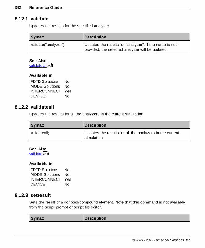
Reference Guide342
© 2003 - 2012 Lumerical Solutions, Inc
8.12.1 validate
Updates the results for the specified analyzer.
Syntax Description
validate("analyzer"); Updates the results for "analyzer". If the name is notprovided, the selected analyzer will be updated.
See Also validateall
Available in
FDTD SolutionsMODE SolutionsINTERCONNECTDEVICE
NoNoYesNo
8.12.2 validateall
Updates the results for all the analyzers in the current simulation.
Syntax Description
validateall; Updates the results for all the analyzers in the currentsimulation.
See Also validate
Available in
FDTD SolutionsMODE SolutionsINTERCONNECTDEVICE
NoNoYesNo
8.12.3 setresult
Sets the result of a scripted/compound element. Note that this command is not availablefrom the script prompt or script file editor.
Syntax Description
342
342

Scripting Language 343
© 2003 - 2012 Lumerical Solutions, Inc
setresult("result",value); Sets the "result" for the scripted/compound element to thespecified value.
setresult("result",value,"kind(unit)");
Sets the "result" for the scripted/compound element to thespecified value with the given description. Note that unitsshould be placed in parenthesis.
setresult("result",x,y,"xtitle",'y title');
Sets the x, y parameters of the "result" for the scripted/compound element. This is useful for visualization.
See Also getresult
Available in
FDTD SolutionsMODE SolutionsINTERCONNECTDEVICE
NoNoYesNo
8.12.4 getresult
See getresult .
8.12.5 popportdata
Extract the first available data value from the input port.
Syntax Description
data_out = popportdata('input_port");
Returns the first available data value from "input_port".
See Also pushportdata , cloneportdata , portdatasize
Available in
FDTD SolutionsMODE SolutionsINTERCONNECTDEVICE
NoNoYesNo
350
350
344 344 344
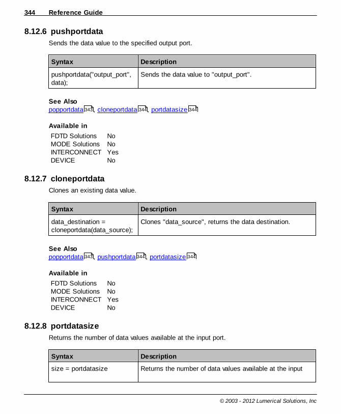
Reference Guide344
© 2003 - 2012 Lumerical Solutions, Inc
8.12.6 pushportdata
Sends the data value to the specified output port.
Syntax Description
pushportdata("output_port",data);
Sends the data value to "output_port".
See Also popportdata , cloneportdata , portdatasize
Available in
FDTD SolutionsMODE SolutionsINTERCONNECTDEVICE
NoNoYesNo
8.12.7 cloneportdata
Clones an existing data value.
Syntax Description
data_destination =cloneportdata(data_source);
Clones "data_source", returns the data destination.
See Also popportdata , pushportdata , portdatasize
Available in
FDTD SolutionsMODE SolutionsINTERCONNECTDEVICE
NoNoYesNo
8.12.8 portdatasize
Returns the number of data values available at the input port.
Syntax Description
size = portdatasize Returns the number of data values available at the input
343 344 344
343 344 344

Scripting Language 345
© 2003 - 2012 Lumerical Solutions, Inc
("input_port"); port.
See Also popportdata , pushportdata , cloneportdata
Available in
FDTD SolutionsMODE SolutionsINTERCONNECTDEVICE
NoNoYesNo
8.12.9 setsparameter
Sets the s-parameters between output port and input port.
Syntax Description
setsparameter("output_port","input_port", "constant",value);
Sets the s-parameter between "output_port" and"input_port" as a single complex constant value (frequencyindependent).
setsparameter("output_port","mode_1", "input_port", "mode_2","constant", value);
Sets the s-parameter between "mode_1" at "output_port"and "mode_2" at "input_port" as a single complex constantvalue (frequency independent).
setsparameter("output_port","input_port", "transmission",transmission);
Sets the s-parameter between "output_port" and"input_port", where the transmission is a matrix with 3columns: frequency (Hz), amplitude and angle (rad). Thenumber of rows of the matrix is the number of frequencypoints. If only two columns are provided, it is assume thatthe angle values are zero.
setsparameter("output_port","mode_1", "input_port", "mode_2","transmission",transmission);
Sets the s-parameter between "mode_1" at "output_port"and "mode_2" at "input_port", where the transmission is amatrix with 3 columns: frequency (Hz), amplitude andangle (rad). The number of rows of the matrix is the numberof frequency points. If only two columns are provided, it isassume that the angle values are zero.
343 344 344

Reference Guide346
© 2003 - 2012 Lumerical Solutions, Inc
setsparameter("output_port","input_port", "propagation",propagation, length);
Sets the frequency dependent propagation parametersbetween between "output_port" and "input_port", where thepropagation is a matrix with up to 5 columns columns:frequency (Hz), absorption (dB/m), effective index, groupvelocity (m/s) and disperstion (m/s/s). The number of rowsof the matrix is the number of frequency points. Groupvelocity and dispersion are optional. The length (m) is thepropagation length.
setsparameter("output_port","mode_1", "input_port", "mode_2","propagation", propagation,length);
Sets the s-parameter between "mode_1" at "output_port"and "mode_2" at "input_port", where the propagation is amatrix with up to 5 columns columns: frequency (Hz),absorption (dB/m), effective index, group velocity (m/s) anddisperstion (m/s/s). The number of rows of the matrix is thenumber of frequency points. Group velocity and dispersionare optional. The length (m) is the propagation length.
Available in
FDTD SolutionsMODE SolutionsINTERCONNECTDEVICE
NoNoYesNo
8.12.10 setfir
Initialize a FIR filter using the current s-parameters.
Syntax Description
setfir("window",taps); Initialize a FIR filter (with the specified number of taps)using the current s-parameters. "window" is the windowfunction used by the FIR. The options are: "rectangular","hamming", "hanning".
See Also setsparameter
Available in
FDTD SolutionsMODE SolutionsINTERCONNECTDEVICE
NoNoYesNo
345
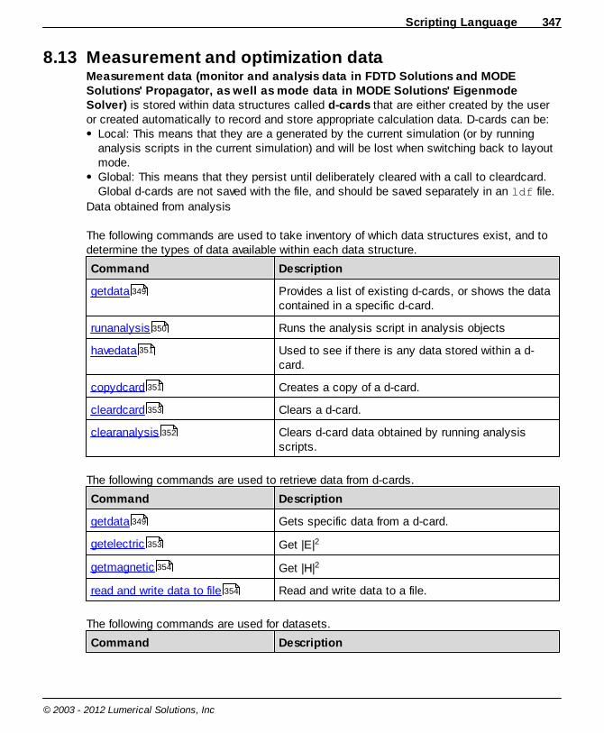
Scripting Language 347
© 2003 - 2012 Lumerical Solutions, Inc
8.13 Measurement and optimization dataMeasurement data (monitor and analysis data in FDTD Solutions and MODESolutions' Propagator, as well as mode data in MODE Solutions' EigenmodeSolver) is stored within data structures called d-cards that are either created by the useror created automatically to record and store appropriate calculation data. D-cards can be:
Local: This means that they are a generated by the current simulation (or by runninganalysis scripts in the current simulation) and will be lost when switching back to layoutmode.Global: This means that they persist until deliberately cleared with a call to cleardcard.Global d-cards are not saved with the file, and should be saved separately in an ldf file.
Data obtained from analysis
The following commands are used to take inventory of which data structures exist, and todetermine the types of data available within each data structure.
Command Description
getdata Provides a list of existing d-cards, or shows the datacontained in a specific d-card.
runanalysis Runs the analysis script in analysis objects
havedata Used to see if there is any data stored within a d-card.
copydcard Creates a copy of a d-card.
cleardcard Clears a d-card.
clearanalysis Clears d-card data obtained by running analysisscripts.
The following commands are used to retrieve data from d-cards.
Command Description
getdata Gets specific data from a d-card.
getelectric Get |E|2
getmagnetic Get |H|2
read and write data to file Read and write data to a file.
The following commands are used for datasets.
Command Description
349
350
351
351
353
352
349
353
354
354
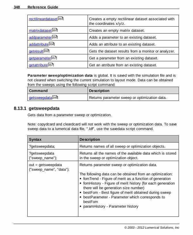
Reference Guide348
© 2003 - 2012 Lumerical Solutions, Inc
rectilineardataset Creates a empty rectilinear dataset associated withthe coordinates x/y/z.
matrixdataset Creates an empty matrix dataset.
addparameter Adds a parameter to an existing dataset.
addattribute Adds an attribute to an existing dataset.
getresult Gets the dataset results from a monitor or analyzer.
getparameter Get a parameter from an existing dataset.
getattribute Get an attribute from an existing dataset.
Parameter sweep/optimization data is global. It is saved with the simulation file and isnot cleared when switching the current simulation to layout mode. Data can be obtainedfrom the sweeps using the following script command:
Command Description
getsweepdata Returns parameter sweep or optimization data.
8.13.1 getsweepdata
Gets data from a parameter sweep or optimization.
Note: copydcard and cleardcard will not work with the sweep or optimization data. To savesweep data to a lumerical data file, ".ldf", use the savedata script command.
Syntax Description
?getsweepdata; Returns names of all sweep or optimization objects.
?getsweepdata("sweep_name");
Returns all the names of the available data which is storedin the sweep or optimization object.
out = getsweepdata("sweep_name", "data");
Returns parameter sweep or optimization data.
The following data can be obtained from an optimization:fomTrend - Figure of merit as a function of generationfomHistory - Figure of merit history (for each generationthere will be generation size number)bestFom - Best figure of merit obtained during sweepbestParameter - Parameter which corresponds tobestFomparamHistory - Parameter history
354
355
356
356
350
357
357
348

Scripting Language 349
© 2003 - 2012 Lumerical Solutions, Inc
For a parameter sweep, this command returns bothparameters and results.
See Alsogetdata , savedata , runsweep
Available in
FDTD SolutionsMODE SolutionsINTERCONNECTDEVICE
YesYesYesYes
8.13.2 getdata
Get data from the simulation. Remember to run the simulation before using getdata.
Syntax Description
?getdata; Returns names of all objects with data.
?getdata("monitor") Returns list of of data within the simulation object.
out = getdata( "monitor","dataname");
Gets data from a monitor. For example, you can useEx = getdata("monitor1","Ex");
to get the Ex field data from monitor1.
out = getdata( "dcard","dataname", option);
The optional argument, option, can have a value of 1 or 2. Ifit is 2, the data is unfolded where possible according to thesymmetry or anti-symmetric boundaries if it comes from amonitor that intersect such a boundary at x min, y min or zmin. The default value of option is 2.
For Propagator simulations in MODE Solutions, thisoptions also allow users to choose whether to expand thedata to the correct size for dimensions where the fieldcomponent is zero. Option 1 will return a singleton value of0 for the field component in that dimension, and option 2will return a matrix (composed of zeros) that matches thesize of the other field components.
See AlsoMeasurements , havedata , getelectric , getmagnetic , nonorm , cwnorm ,getsweepdata
349 174 319
347 351 353 354 324 325
348

Reference Guide350
© 2003 - 2012 Lumerical Solutions, Inc
Available in
FDTD SolutionsMODE SolutionsINTERCONNECTDEVICE
YesYesYesYes
8.13.3 getresult
Gets the dataset results from a monitor or analysis group. For getting results that arescalar matrices, see getdata .
Syntax Description
?getresult("monitor_name"); Returns the names of all the results for the monitor. All thedataset and scalar matrix results will be returned in thiscase.
R = getresult("monitor_name","R");
Returns the result R from the monitor. R is a dataset.
See Alsorectilineardataset , matrixdataset , getattribute , addattribute , "." operator ,visualize
Available in
FDTD SolutionsMODE SolutionsINTERCONNECTDEVICE
Version 8+NoYesNo
8.13.4 runanalysis
Runs the analysis script in analysis objects.
Note: Scripts that already have data are not re-run; to re-run a script, first clear data usingclearanalysis.
Syntax Description
runanalysis; Runs the analysis scripts in all analysis objects in thesimulation file.This function does not return any data.
runanalysis("group name"); Runs the analysis script in the analysis object named
349
354 355 357 356 219
259

Scripting Language 351
© 2003 - 2012 Lumerical Solutions, Inc
"group name".This function does not return any data.
See Also run , getdata , havedata , clearanalysis , runsetup
Available in
FDTD SolutionsMODE SolutionsINTERCONNECTDEVICE
YesYesYesYes
8.13.5 havedata
Used to see if there is any data stored within a d-card (note that only raw data isconsidered here, this does not include expanded data or calculated data from themonitors).
Syntax Description
havedata; Returns 1 if any of the d-cards currently in memory haveraw data, and 0 if none of the d-cards have any raw data.
havedata("name"); Returns 1 if the d-card named "name" has raw data, and 0if it does not have any raw data.
havedata("name","data"); Returns 1 if the d-card named "name" has the raw datanamed "data", and 0 if it does not have any raw data.
See AlsoMeasurements , getdata , copydcard , cleardcard , workspace
Available in
FDTD SolutionsMODE SolutionsINTERCONNECTDEVICE
YesYesNoYes
8.13.6 copydcard
Will create a global copy of any d-card currently in memory.
Syntax Description
317 349 351 352 295
347 349 351 353 189
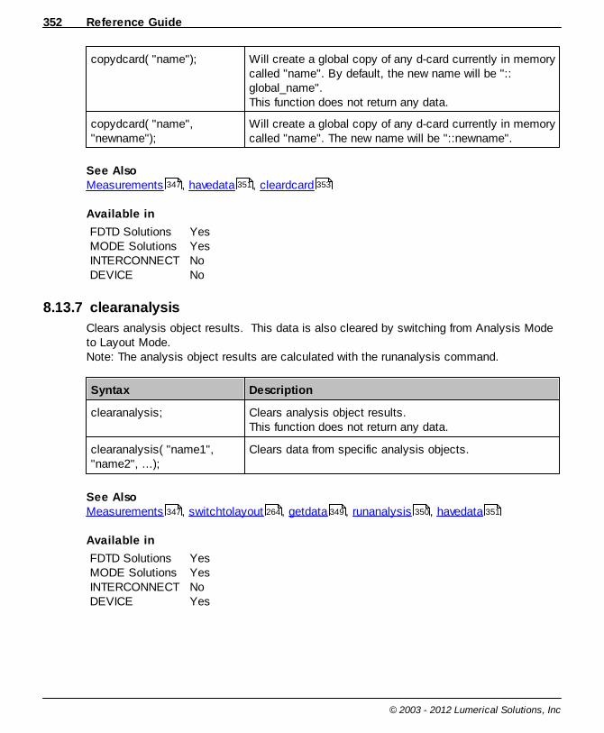
Reference Guide352
© 2003 - 2012 Lumerical Solutions, Inc
copydcard( "name"); Will create a global copy of any d-card currently in memorycalled "name". By default, the new name will be "::global_name".This function does not return any data.
copydcard( "name","newname");
Will create a global copy of any d-card currently in memorycalled "name". The new name will be "::newname".
See AlsoMeasurements , havedata , cleardcard
Available in
FDTD SolutionsMODE SolutionsINTERCONNECTDEVICE
YesYesNoNo
8.13.7 clearanalysis
Clears analysis object results. This data is also cleared by switching from Analysis Modeto Layout Mode.Note: The analysis object results are calculated with the runanalysis command.
Syntax Description
clearanalysis; Clears analysis object results. This function does not return any data.
clearanalysis( "name1","name2", ...);
Clears data from specific analysis objects.
See AlsoMeasurements , switchtolayout , getdata , runanalysis , havedata
Available in
FDTD SolutionsMODE SolutionsINTERCONNECTDEVICE
YesYesNoYes
347 351 353
347 264 349 350 351
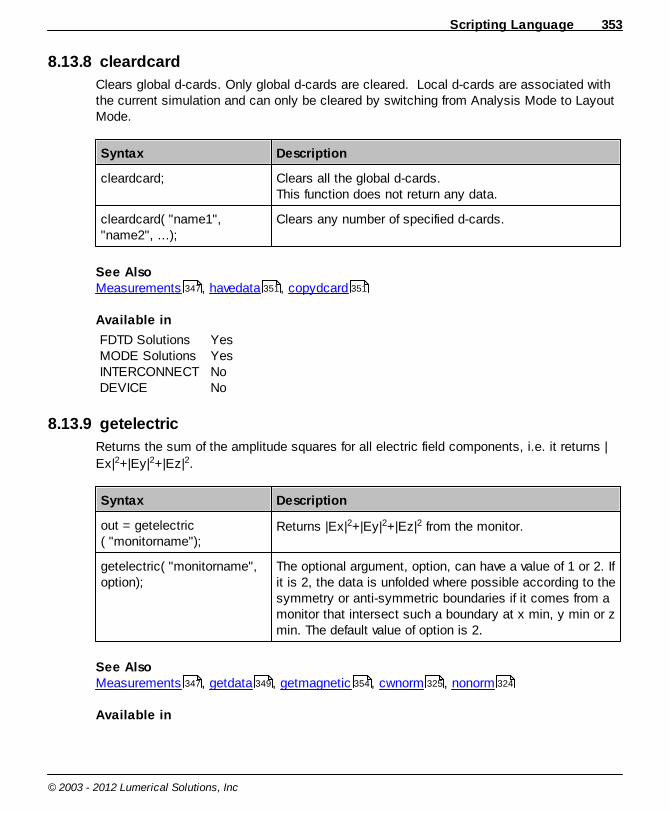
Scripting Language 353
© 2003 - 2012 Lumerical Solutions, Inc
8.13.8 cleardcard
Clears global d-cards. Only global d-cards are cleared. Local d-cards are associated withthe current simulation and can only be cleared by switching from Analysis Mode to LayoutMode.
Syntax Description
cleardcard; Clears all the global d-cards. This function does not return any data.
cleardcard( "name1","name2", ...);
Clears any number of specified d-cards.
See AlsoMeasurements , havedata , copydcard
Available in
FDTD SolutionsMODE SolutionsINTERCONNECTDEVICE
YesYesNoNo
8.13.9 getelectric
Returns the sum of the amplitude squares for all electric field components, i.e. it returns |
Ex|2+|Ey|2+|Ez|2.
Syntax Description
out = getelectric( "monitorname");
Returns |Ex|2+|Ey|2+|Ez|2 from the monitor.
getelectric( "monitorname",option);
The optional argument, option, can have a value of 1 or 2. Ifit is 2, the data is unfolded where possible according to thesymmetry or anti-symmetric boundaries if it comes from amonitor that intersect such a boundary at x min, y min or zmin. The default value of option is 2.
See AlsoMeasurements , getdata , getmagnetic , cwnorm , nonorm
Available in
347 351 351
347 349 354 325 324

Reference Guide354
© 2003 - 2012 Lumerical Solutions, Inc
FDTD SolutionsMODE SolutionsINTERCONNECTDEVICE
YesYesNoNo
8.13.10 getmagnetic
Returns the sum of the amplitude squares for all magnetic field components, i.e. it returns |
Hx|2+|Hy|2+|Hz|2.
Syntax Description
out = getmagnetic( "monitorname");
Returns |Hx|2+|Hy|2+|Hz|2 from the monitor.
getmagnetic( "monitorname", option);
The optional argument, option, can have a value of 1 or 2. Ifit is 2, the data is unfolded where possible according to thesymmetry or anti-symmetric boundaries if it comes from amonitor that intersect such a boundary at x min, y min or zmin. The default value of option is 2.
See Also Measurements , getdata , getelectric , cwnorm , nonorm
Available in
FDTD SolutionsMODE SolutionsINTERCONNECTDEVICE
YesYesNoNo
8.13.11 Read and write data to files
Please see the following section for file I/O commands.System level commands: File input and output
8.13.12 rectilineardataset
Creates an empty rectilinear dataset that is associate with the x/y/z coordinates (ex. E andH fields). Like matrix datasets, rectilinear datasets can be parameterized, and can containan arbitrary number of attributes (see addattribute) and parameters (see addparameter)
.
For datasets that are not associated with the x/y/z coordinates (ex. transmission as afunction of frequency), see matrixdataset .
347 349 353 325 324
156
356
356
355
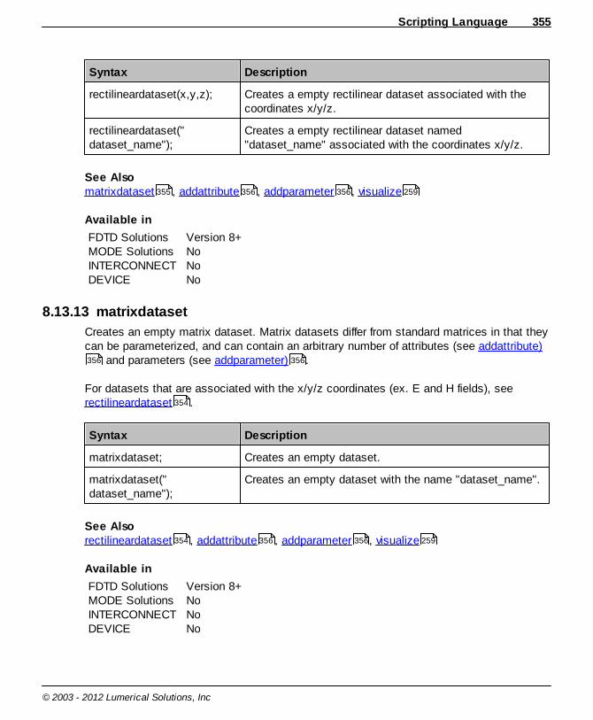
Scripting Language 355
© 2003 - 2012 Lumerical Solutions, Inc
Syntax Description
rectilineardataset(x,y,z); Creates a empty rectilinear dataset associated with thecoordinates x/y/z.
rectilineardataset("dataset_name");
Creates a empty rectilinear dataset named"dataset_name" associated with the coordinates x/y/z.
See Alsomatrixdataset , addattribute , addparameter , visualize
Available in
FDTD SolutionsMODE SolutionsINTERCONNECTDEVICE
Version 8+NoNoNo
8.13.13 matrixdataset
Creates an empty matrix dataset. Matrix datasets differ from standard matrices in that theycan be parameterized, and can contain an arbitrary number of attributes (see addattribute)
and parameters (see addparameter) .
For datasets that are associated with the x/y/z coordinates (ex. E and H fields), see rectilineardataset .
Syntax Description
matrixdataset; Creates an empty dataset.
matrixdataset("dataset_name");
Creates an empty dataset with the name "dataset_name".
See Alsorectilineardataset , addattribute , addparameter , visualize
Available in
FDTD SolutionsMODE SolutionsINTERCONNECTDEVICE
Version 8+NoNoNo
355 356 356 259
356 356
354
354 356 356 259

Reference Guide356
© 2003 - 2012 Lumerical Solutions, Inc
8.13.14 addparameter
Adds a parameter to an existing dataset.
Syntax Description
R.addparameter("p_name",p);
Adds the parameter p to the existing dataset R.
R.addparameter("p1_name",p1, "p2_name", p2);
Adds the parameter1 p1 and p2 to the existing dataset R.Here, p1 and p2 must be interdependent. For example, p1= frequency and p2 = wavelength. Parameters that are notinterdependent must be added separately.
matrixdataset , rectilineardataset , addattribute , visualize
Available in
FDTD SolutionsMODE SolutionsINTERCONNECTDEVICE
Version 8+NoNoNo
8.13.15 addattribute
Adds an attribute to an existing dataset.
Syntax Description
R.addattribute("a_name", a); Adds the attribute a to the existing dataset R.
R.addattribute("a_vector",a_1, a_2, a_3);
Adds the vector attribute a_vector to the existing datasetR. The components of the vector are a_1, a_2 and a_3
See Alsomatrixdataset , addattribute , addparameter , visualize
Available in
FDTD SolutionsMODE SolutionsINTERCONNECTDEVICE
Version 8+NoNoNo
355 354 356 259
355 356 356 259

Scripting Language 357
© 2003 - 2012 Lumerical Solutions, Inc
8.13.16 getparameter
Get a parameter from an existing dataset.
Syntax Description
?getparameter(R); Returns the names of all the parameters in the dataset R.
Parameter = R.getparameter("p");
Retrieves the parameter p from the existing dataset R. Theresult "Parameter" is a scalar matrix.
Parameter = getparameter(R,"p");
Retrieves the parameter p from the existing dataset R. Theresult "Parameter" is a scalar matrix.
matrixdataset , rectilineardataset , "." operator , getresult , getattribute ,visualize
Available in
FDTD SolutionsMODE SolutionsINTERCONNECTDEVICE
Version 8+NoNoNo
8.13.17 getattribute
Get an attribute from an existing dataset.
Syntax Description
?getattribute(R); Returns the names of all the attributes in the dataset R.
Attribute = R.getattribute("a");
Retrieves the attribute a from the existing dataset R. Theresult "Attribute" is a scalar matrix.
Attribute = getparameter(R,"a");
Retrieves the attribute a from the existing dataset R. Theresult "Attribute" is a scalar matrix.
matrixdataset , rectilineardataset , "." operator , getresult , getparameter ,visualize
Available in
FDTD SolutionsMODE SolutionsINTERCONNECTDEVICE
Version 8+NoNoNo
355 354 219 350 357
259
355 354 219 350 357
259
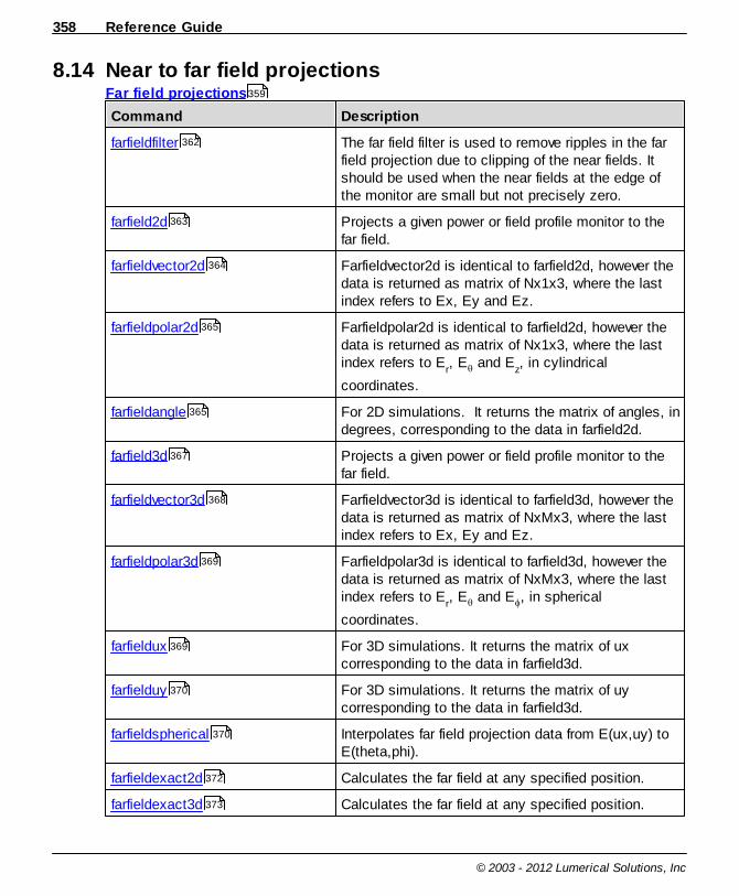
Reference Guide358
© 2003 - 2012 Lumerical Solutions, Inc
8.14 Near to far field projectionsFar field projections
Command Description
farfieldfilter The far field filter is used to remove ripples in the farfield projection due to clipping of the near fields. Itshould be used when the near fields at the edge ofthe monitor are small but not precisely zero.
farfield2d Projects a given power or field profile monitor to thefar field.
farfieldvector2d Farfieldvector2d is identical to farfield2d, however thedata is returned as matrix of Nx1x3, where the lastindex refers to Ex, Ey and Ez.
farfieldpolar2d Farfieldpolar2d is identical to farfield2d, however thedata is returned as matrix of Nx1x3, where the lastindex refers to E
r, E and E
z, in cylindrical
coordinates.
farfieldangle For 2D simulations. It returns the matrix of angles, indegrees, corresponding to the data in farfield2d.
farfield3d Projects a given power or field profile monitor to thefar field.
farfieldvector3d Farfieldvector3d is identical to farfield3d, however thedata is returned as matrix of NxMx3, where the lastindex refers to Ex, Ey and Ez.
farfieldpolar3d Farfieldpolar3d is identical to farfield3d, however thedata is returned as matrix of NxMx3, where the lastindex refers to E
r, E and E , in spherical
coordinates.
farfieldux For 3D simulations. It returns the matrix of uxcorresponding to the data in farfield3d.
farfielduy For 3D simulations. It returns the matrix of uycorresponding to the data in farfield3d.
farfieldspherical Interpolates far field projection data from E(ux,uy) toE(theta,phi).
farfieldexact2d Calculates the far field at any specified position.
farfieldexact3d Calculates the far field at any specified position.
359
362
363
364
365
365
367
368
369
369
370
370
372
373
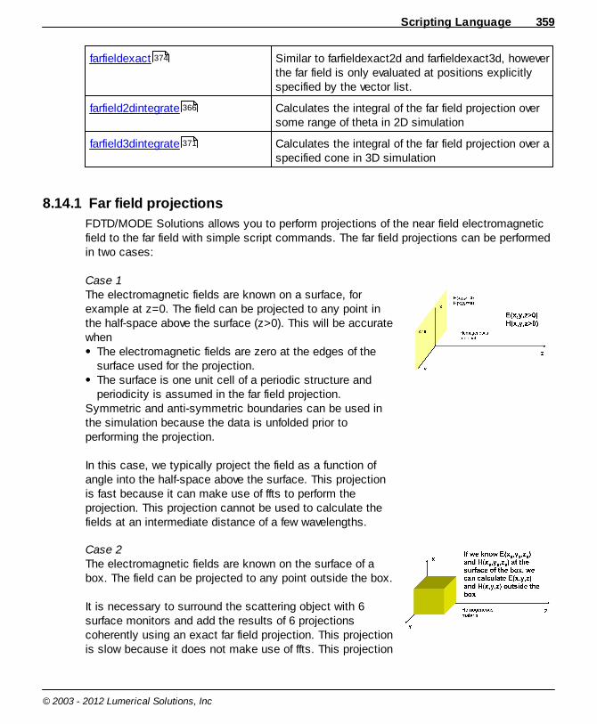
Scripting Language 359
© 2003 - 2012 Lumerical Solutions, Inc
farfieldexact Similar to farfieldexact2d and farfieldexact3d, howeverthe far field is only evaluated at positions explicitlyspecified by the vector list.
farfield2dintegrate Calculates the integral of the far field projection oversome range of theta in 2D simulation
farfield3dintegrate Calculates the integral of the far field projection over aspecified cone in 3D simulation
8.14.1 Far field projections
FDTD/MODE Solutions allows you to perform projections of the near field electromagneticfield to the far field with simple script commands. The far field projections can be performedin two cases:
Case 1The electromagnetic fields are known on a surface, forexample at z=0. The field can be projected to any point inthe half-space above the surface (z>0). This will be accuratewhen
The electromagnetic fields are zero at the edges of thesurface used for the projection.The surface is one unit cell of a periodic structure andperiodicity is assumed in the far field projection.
Symmetric and anti-symmetric boundaries can be used inthe simulation because the data is unfolded prior toperforming the projection.
In this case, we typically project the field as a function ofangle into the half-space above the surface. This projectionis fast because it can make use of ffts to perform theprojection. This projection cannot be used to calculate thefields at an intermediate distance of a few wavelengths.
Case 2The electromagnetic fields are known on the surface of abox. The field can be projected to any point outside the box.
It is necessary to surround the scattering object with 6surface monitors and add the results of 6 projectionscoherently using an exact far field projection. This projectionis slow because it does not make use of ffts. This projection
374
366
371

Reference Guide360
© 2003 - 2012 Lumerical Solutions, Inc
can be used to calculate the fields as close as a fewwavelengths from where they were recorded.
Field normalizationThe far field projection functions return either the complex electric field E or electric field
intensity |E|2 at a distance of 1m. To scale the field to a different distance we canrecognize that the E and |E| 2 scale as shown in the following table.
Electric field scaling Electric field intensity scaling
2D RERE /)( 0
r
ErE
22 )1(
)(
3D RERE /)( 0
2
22 )1(
)(r
ErE
Power IntegralsWe often want to integrate power over a given solid angle in the far field. There are 2 waysthis can be done
1. We integrate the fraction of total electric field intensity (|E|2) over the solid angle that weare interested in, and multiply by the normalized power transmission through the monitorin the near field.
2. We calculate the Poynting vector in the far field and integrate the power over a givensolid angle. We then normalize to the original source power. In the far field, we can useplane wave relationships between E and H. Therefore the Poynting vector is simply
2
0
0 EnP
Both methods will give the same result.
Coordinate SystemsThe 3D far field projections use the direction cosine coordinate system to specify far fieldpositions. Direction cosine units provide a convenient way to specify locations on ahemispherical surface, which is what the far field projections typically return. Also, whencalculating vector far field field data (to obtain polarization information), you can choose toreturn the data using cartesian or spherical coordinates. For more information, please seethe Coordinate systems page.
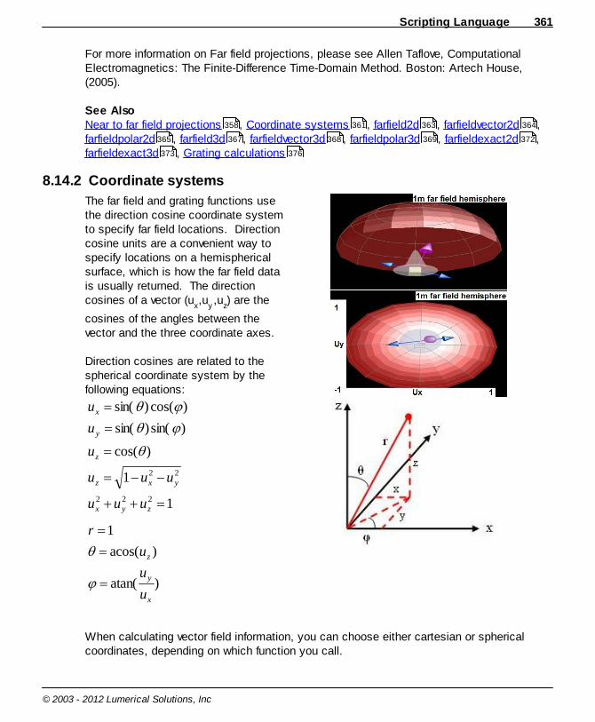
Scripting Language 361
© 2003 - 2012 Lumerical Solutions, Inc
For more information on Far field projections, please see Allen Taflove, ComputationalElectromagnetics: The Finite-Difference Time-Domain Method. Boston: Artech House,(2005).
See AlsoNear to far field projections , Coordinate systems , farfield2d , farfieldvector2d ,farfieldpolar2d , farfield3d , farfieldvector3d , farfieldpolar3d , farfieldexact2d ,farfieldexact3d , Grating calculations
8.14.2 Coordinate systems
The far field and grating functions usethe direction cosine coordinate systemto specify far field locations. Directioncosine units are a convenient way tospecify locations on a hemisphericalsurface, which is how the far field datais usually returned. The directioncosines of a vector (u
x,u
y,u
z) are the
cosines of the angles between thevector and the three coordinate axes.
Direction cosines are related to thespherical coordinate system by thefollowing equations:
1
1
)cos(
)sin()sin(
)cos()sin(
222
22
zyx
yxz
z
y
x
uuu
uuu
u
u
u
)atan(
)acos(
1
x
y
z
u
u
u
r
When calculating vector field information, you can choose either cartesian or sphericalcoordinates, depending on which function you call.
358 361 363 364
365 367 368 369 372
373 376

Reference Guide362
© 2003 - 2012 Lumerical Solutions, Inc
Cartesian coordinates Spherical coordinates
Note on performing integralsWe typically want to perform integrals in spherical coordinates such as the following
ddRPpower )sin(),( 2
where P is the poynting vector and R is the radius.
When changing integration variables from ( , ) to (ux,u
y), it can be shown that
cos),(
sin),(
2
2
yxyx
duduRuuP
ddRPpower
Care must be taken to avoid numerical errors due to the cos( ) term.
See AlsoFar field projections ,Grating calculations
8.14.3 farfieldfilter
The far field filter is used to remove ripples in the far field projection due to clipping of thenear fields. It should be used when the near fields at the edge of the monitor are small butnot precisely zero. The far field filter has a single input parameter, which is a numberbetween 0 and 1. By default, it is 0, which turns the filter off. This filter is applied to all farfield projections.
359 376
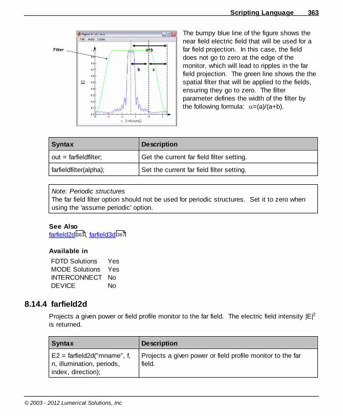
Scripting Language 363
© 2003 - 2012 Lumerical Solutions, Inc
The bumpy blue line of the figure shows thenear field electric field that will be used for afar field projection. In this case, the fielddoes not go to zero at the edge of themonitor, which will lead to ripples in the farfield projection. The green line shows the thespatial filter that will be applied to the fields,ensuring they go to zero. The filterparameter defines the width of the filter bythe following formula: =(a)/(a+b).
Syntax Description
out = farfieldfilter; Get the current far field filter setting.
farfieldfilter(alpha); Set the current far field filter setting.
Note: Periodic structuresThe far field filter option should not be used for periodic structures. Set it to zero whenusing the 'assume periodic' option.
See Alsofarfield2d , farfield3d
Available in
FDTD SolutionsMODE SolutionsINTERCONNECTDEVICE
YesYesNoNo
8.14.4 farfield2d
Projects a given power or field profile monitor to the far field. The electric field intensity |E|2
is returned.
Syntax Description
E2 = farfield2d("mname", f,n, illumination, periods,index, direction);
Projects a given power or field profile monitor to the farfield.
363 367
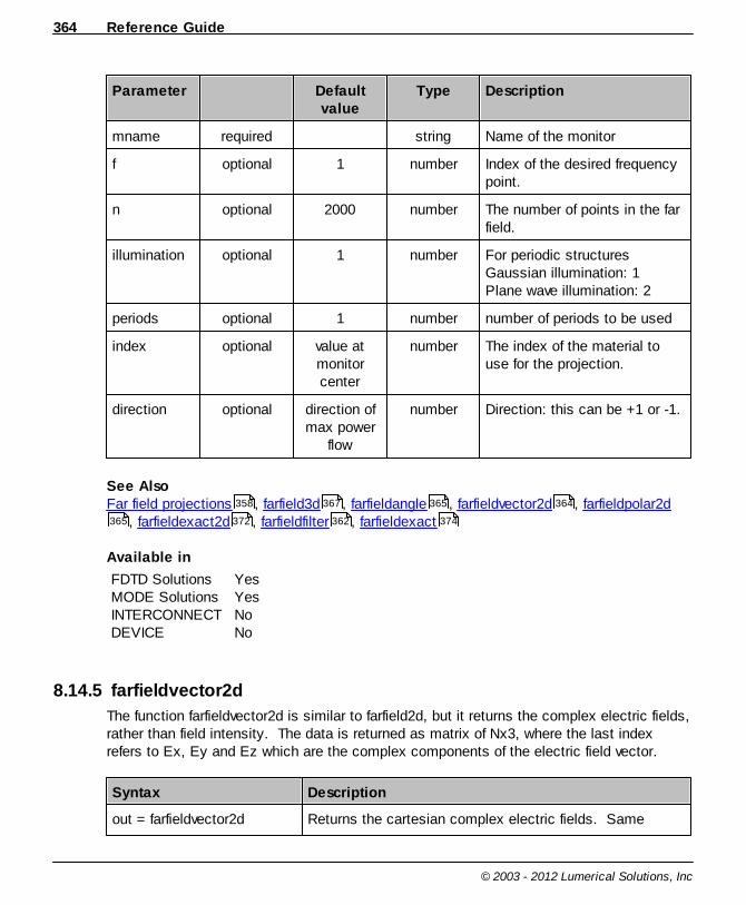
Reference Guide364
© 2003 - 2012 Lumerical Solutions, Inc
Parameter Defaultvalue
Type Description
mname required string Name of the monitor
f optional 1 number Index of the desired frequencypoint.
n optional 2000 number The number of points in the farfield.
illumination optional 1 number For periodic structuresGaussian illumination: 1Plane wave illumination: 2
periods optional 1 number number of periods to be used
index optional value atmonitorcenter
number The index of the material touse for the projection.
direction optional direction ofmax power
flow
number Direction: this can be +1 or -1.
See AlsoFar field projections , farfield3d , farfieldangle , farfieldvector2d , farfieldpolar2d
, farfieldexact2d , farfieldfilter , farfieldexact
Available in
FDTD SolutionsMODE SolutionsINTERCONNECTDEVICE
YesYesNoNo
8.14.5 farfieldvector2d
The function farfieldvector2d is similar to farfield2d, but it returns the complex electric fields,rather than field intensity. The data is returned as matrix of Nx3, where the last indexrefers to Ex, Ey and Ez which are the complex components of the electric field vector.
Syntax Description
out = farfieldvector2d Returns the cartesian complex electric fields. Same
358 367 365 364
365 372 362 374
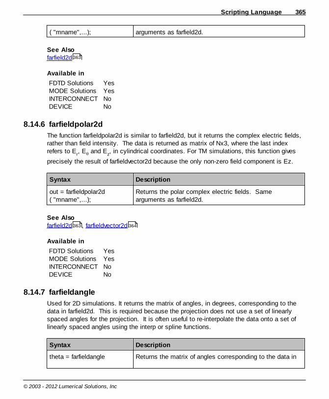
Scripting Language 365
© 2003 - 2012 Lumerical Solutions, Inc
( "mname",...); arguments as farfield2d.
See Alsofarfield2d
Available in
FDTD SolutionsMODE SolutionsINTERCONNECTDEVICE
YesYesNoNo
8.14.6 farfieldpolar2d
The function farfieldpolar2d is similar to farfield2d, but it returns the complex electric fields,rather than field intensity. The data is returned as matrix of Nx3, where the last indexrefers to E
r, E and E
z, in cylindrical coordinates. For TM simulations, this function gives
precisely the result of farfieldvector2d because the only non-zero field component is Ez.
Syntax Description
out = farfieldpolar2d( "mname",...);
Returns the polar complex electric fields. Samearguments as farfield2d.
See Alsofarfield2d , farfieldvector2d
Available in
FDTD SolutionsMODE SolutionsINTERCONNECTDEVICE
YesYesNoNo
8.14.7 farfieldangle
Used for 2D simulations. It returns the matrix of angles, in degrees, corresponding to thedata in farfield2d. This is required because the projection does not use a set of linearlyspaced angles for the projection. It is often useful to re-interpolate the data onto a set oflinearly spaced angles using the interp or spline functions.
Syntax Description
theta = farfieldangle Returns the matrix of angles corresponding to the data in
363
363 364
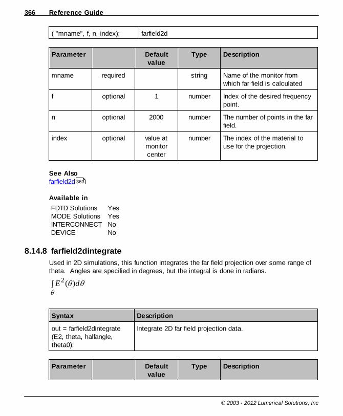
Reference Guide366
© 2003 - 2012 Lumerical Solutions, Inc
( "mname", f, n, index); farfield2d
Parameter Defaultvalue
Type Description
mname required string Name of the monitor fromwhich far field is calculated
f optional 1 number Index of the desired frequencypoint.
n optional 2000 number The number of points in the farfield.
index optional value atmonitorcenter
number The index of the material touse for the projection.
See Alsofarfield2d
Available in
FDTD SolutionsMODE SolutionsINTERCONNECTDEVICE
YesYesNoNo
8.14.8 farfield2dintegrate
Used in 2D simulations, this function integrates the far field projection over some range oftheta. Angles are specified in degrees, but the integral is done in radians.
dE )(2
Syntax Description
out = farfield2dintegrate(E2, theta, halfangle,theta0);
Integrate 2D far field projection data.
Parameter Defaultvalue
Type Description
363

Scripting Language 367
© 2003 - 2012 Lumerical Solutions, Inc
E2 required matrix E field data from farfield2d
theta required matrix Theta from farfieldangle
halfangle optional 90 vector Half angle (in degrees) of theintegration region. Must havesame length as theta0 orlength 1.
theta0 optional 0 vector Center angle (in degrees) thetaof the integration region. Musthave same length as halfangleor length 1.
See AlsoNear to far field projections , farfield2d , farfieldangle
Available in
FDTD SolutionsMODE SolutionsINTERCONNECTDEVICE
YesYesNoNo
8.14.9 farfield3d
Projects a given power or field profile monitor to the far field. The electric field intensity |E|2
is returned.
Syntax Description
out = farfield3d("mname",f,na, nb, illumination,periodsa, periodsb, index,direction);
Projects a given power or field profile monitor to the farfield. For directions, when projecting in
x: a is y and b is z y: a is x and b is z z: a is x and b is y
Parameter Defaultvalue
Type Description
mname required string Name of the monitor
f optional 1 number Index of the desired frequencypoint.
na optional 150 number The number of points in the far
358 363 365

Reference Guide368
© 2003 - 2012 Lumerical Solutions, Inc
field.
nb optional 150 number The number of points in the farfield.
illumination optional 1 number For periodic structures.Gaussian illumination: 1Plane wave illumination: 2
periodsa optional 1 number number of periods to be usedfor periodic illumination
periodsb optional 1 number number of periods to be usedfor periodic illumination
index optional value atmonitorcenter
number The index of the material touse for the projection.
direction optional direction ofmax power
flow
number Direction: this can be +1 or -1.
See AlsoFar field projections , farfield2d , farfieldvector3d , farfieldpolar3d , farfieldux ,farfielduy , farfieldexact3d , farfieldfilter
Available in
FDTD SolutionsMODE SolutionsINTERCONNECTDEVICE
YesYesNoNo
8.14.10 farfieldvector3d
The function farfieldvector3d is similar to farfield3d, but it returns the complex electric fields,rather than field intensity. The data is returned as matrix of NxMx3, where N and M arespatial indices and the last index refers to Ex, Ey and Ez. The components Ex, Ey and Ezare the complex components of the electric field vector.
Syntax Description
out = farfieldvector3d( "monitorname",...);
Returns the cartesian complex electric fields. Samearguments as farfield3d.
See Also
358 363 368 369 369
370 373 362
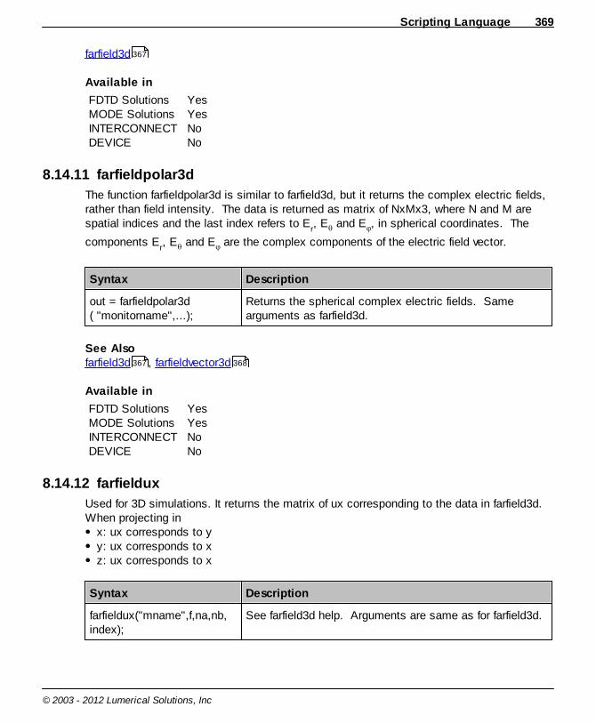
Scripting Language 369
© 2003 - 2012 Lumerical Solutions, Inc
farfield3d
Available in
FDTD SolutionsMODE SolutionsINTERCONNECTDEVICE
YesYesNoNo
8.14.11 farfieldpolar3d
The function farfieldpolar3d is similar to farfield3d, but it returns the complex electric fields,rather than field intensity. The data is returned as matrix of NxMx3, where N and M arespatial indices and the last index refers to E
r, E and E , in spherical coordinates. The
components Er, E and E are the complex components of the electric field vector.
Syntax Description
out = farfieldpolar3d( "monitorname",...);
Returns the spherical complex electric fields. Samearguments as farfield3d.
See Alsofarfield3d , farfieldvector3d
Available in
FDTD SolutionsMODE SolutionsINTERCONNECTDEVICE
YesYesNoNo
8.14.12 farfieldux
Used for 3D simulations. It returns the matrix of ux corresponding to the data in farfield3d.When projecting in
x: ux corresponds to y y: ux corresponds to x z: ux corresponds to x
Syntax Description
farfieldux("mname",f,na,nb,index);
See farfield3d help. Arguments are same as for farfield3d.
367
367 368
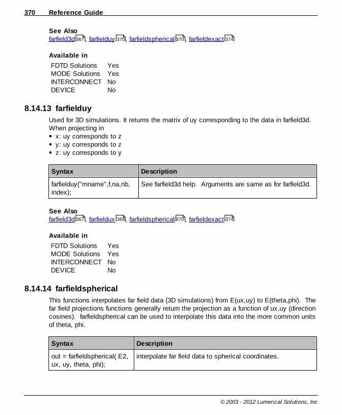
Reference Guide370
© 2003 - 2012 Lumerical Solutions, Inc
See Alsofarfield3d , farfielduy , farfieldspherical , farfieldexact
Available in
FDTD SolutionsMODE SolutionsINTERCONNECTDEVICE
YesYesNoNo
8.14.13 farfielduy
Used for 3D simulations. It returns the matrix of uy corresponding to the data in farfield3d.When projecting in
x: uy corresponds to z y: uy corresponds to z z: uy corresponds to y
Syntax Description
farfielduy("mname",f,na,nb,index);
See farfield3d help. Arguments are same as for farfield3d.
See Alsofarfield3d , farfieldux , farfieldspherical , farfieldexact
Available in
FDTD SolutionsMODE SolutionsINTERCONNECTDEVICE
YesYesNoNo
8.14.14 farfieldspherical
This functions interpolates far field data (3D simulations) from E(ux,uy) to E(theta,phi). Thefar field projections functions generally return the projection as a function of ux,uy (directioncosines). farfieldspherical can be used to interpolate this data into the more common unitsof theta, phi.
Syntax Description
out = farfieldspherical( E2,ux, uy, theta, phi);
interpolate far field data to spherical coordinates.
367 370 370 374
367 369 370 374

Scripting Language 371
© 2003 - 2012 Lumerical Solutions, Inc
Parameter Defaultvalue
Type Description
E2 required matrix E field data from farfield3d
ux required vector ux data from farfieldux
uy required vector uy data from farfielduy
theta required vector theta vector, in degrees. Musthave length L or 1.
phi required vector phi vector, in degrees. Musthave length L or 1.
See AlsoFar field projections , farfield3d , farfieldux , farfielduy
Available in
FDTD SolutionsMODE SolutionsINTERCONNECTDEVICE
YesYesNoNo
8.14.15 farfield3dintegrate
Used in 3D simulations, this function integrates the far field projection over a cone centeredat theta0 and phi0, with a width specified by halfangle. The far field electric field is afunction of the direction cosines (ux,uy), but farfield3dintegrate automatically does thechange of variables. Similarly, angles are specified in degrees, but converted to radiansbefore the integral is calculated.
dduyuxE )sin(,,
2
Syntax Description
out = farfield3dintegrate(E2, ux, uy, halfangle,theta0, phi0);
Integrate 3D far field projection data.
Parameter Defaultvalue
Type Description
358 367 369 370
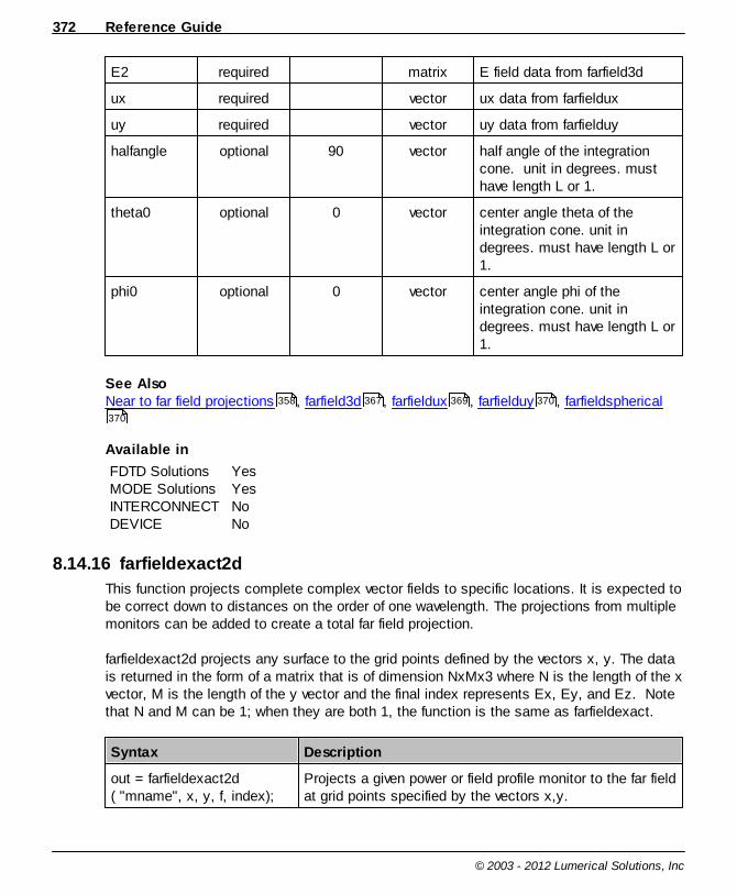
Reference Guide372
© 2003 - 2012 Lumerical Solutions, Inc
E2 required matrix E field data from farfield3d
ux required vector ux data from farfieldux
uy required vector uy data from farfielduy
halfangle optional 90 vector half angle of the integrationcone. unit in degrees. musthave length L or 1.
theta0 optional 0 vector center angle theta of theintegration cone. unit indegrees. must have length L or1.
phi0 optional 0 vector center angle phi of theintegration cone. unit indegrees. must have length L or1.
See AlsoNear to far field projections , farfield3d , farfieldux , farfielduy , farfieldspherical
Available in
FDTD SolutionsMODE SolutionsINTERCONNECTDEVICE
YesYesNoNo
8.14.16 farfieldexact2d
This function projects complete complex vector fields to specific locations. It is expected tobe correct down to distances on the order of one wavelength. The projections from multiplemonitors can be added to create a total far field projection.
farfieldexact2d projects any surface to the grid points defined by the vectors x, y. The datais returned in the form of a matrix that is of dimension NxMx3 where N is the length of the xvector, M is the length of the y vector and the final index represents Ex, Ey, and Ez. Notethat N and M can be 1; when they are both 1, the function is the same as farfieldexact.
Syntax Description
out = farfieldexact2d( "mname", x, y, f, index);
Projects a given power or field profile monitor to the far fieldat grid points specified by the vectors x,y.
358 367 369 370
370
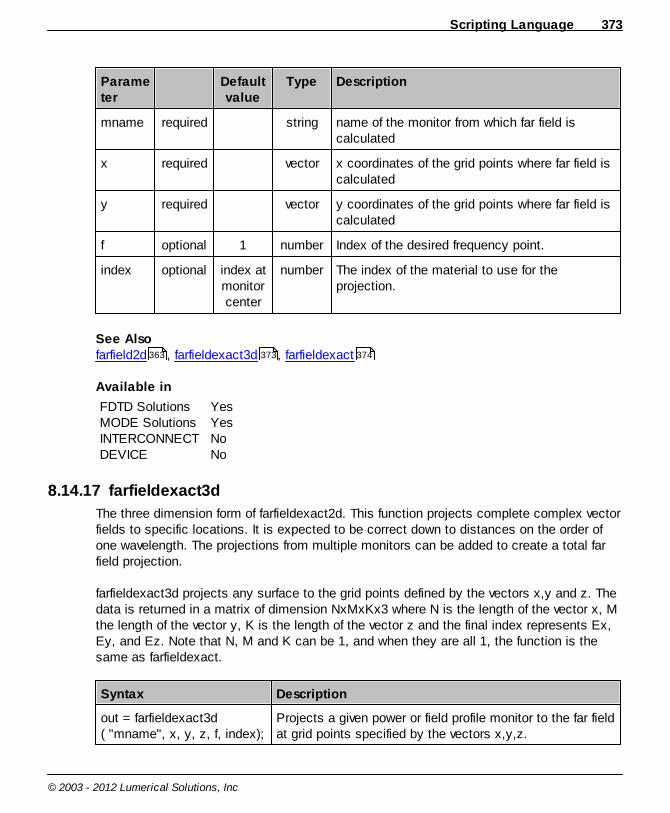
Scripting Language 373
© 2003 - 2012 Lumerical Solutions, Inc
Parameter
Defaultvalue
Type Description
mname required string name of the monitor from which far field iscalculated
x required vector x coordinates of the grid points where far field iscalculated
y required vector y coordinates of the grid points where far field iscalculated
f optional 1 number Index of the desired frequency point.
index optional index atmonitorcenter
number The index of the material to use for theprojection.
See Alsofarfield2d , farfieldexact3d , farfieldexact
Available in
FDTD SolutionsMODE SolutionsINTERCONNECTDEVICE
YesYesNoNo
8.14.17 farfieldexact3d
The three dimension form of farfieldexact2d. This function projects complete complex vectorfields to specific locations. It is expected to be correct down to distances on the order ofone wavelength. The projections from multiple monitors can be added to create a total farfield projection.
farfieldexact3d projects any surface to the grid points defined by the vectors x,y and z. Thedata is returned in a matrix of dimension NxMxKx3 where N is the length of the vector x, Mthe length of the vector y, K is the length of the vector z and the final index represents Ex,Ey, and Ez. Note that N, M and K can be 1, and when they are all 1, the function is thesame as farfieldexact.
Syntax Description
out = farfieldexact3d( "mname", x, y, z, f, index);
Projects a given power or field profile monitor to the far fieldat grid points specified by the vectors x,y,z.
363 373 374

Reference Guide374
© 2003 - 2012 Lumerical Solutions, Inc
Parameter Defaultvalue
Type Description
mname required string name of the monitor from whichfar field is calculated
x required vector x coordinates of the grid pointswhere far field is calculated
y required vector y coordinates of the grid pointswhere far field is calculated
z required vector z coordinates of the grid pointswhere far field is calculated
f optional 1 number Index of the desired frequencypoint.
index optional value atmonitorcenter
number The index of the material touse for the projection.
See Alsofarfield3d , farfieldexact2d , farfieldexact
Available in
FDTD SolutionsMODE SolutionsINTERCONNECTDEVICE
YesYesNoNo
8.14.18 farfieldexact
This function projects complete complex vector fields to specific locations. It is expected tobe correct down to distances on the order of one wavelength. The projections from multiplemonitors can be added to create a total far field projection.
farfieldexact projects any surface fields to a series of points defined by vector lists. The x,y,z coordinates of each evaluation point are taken element-by-element from the vector lists. i.e., the i-th point in a 2D simulation would be at [x(i),y(i)].
3DVectors lists x,y,z must have the same length L or be length 1. The data is returned in amatrix of dimension Lx3. The first index represents positions defined by one element from
367 372 374
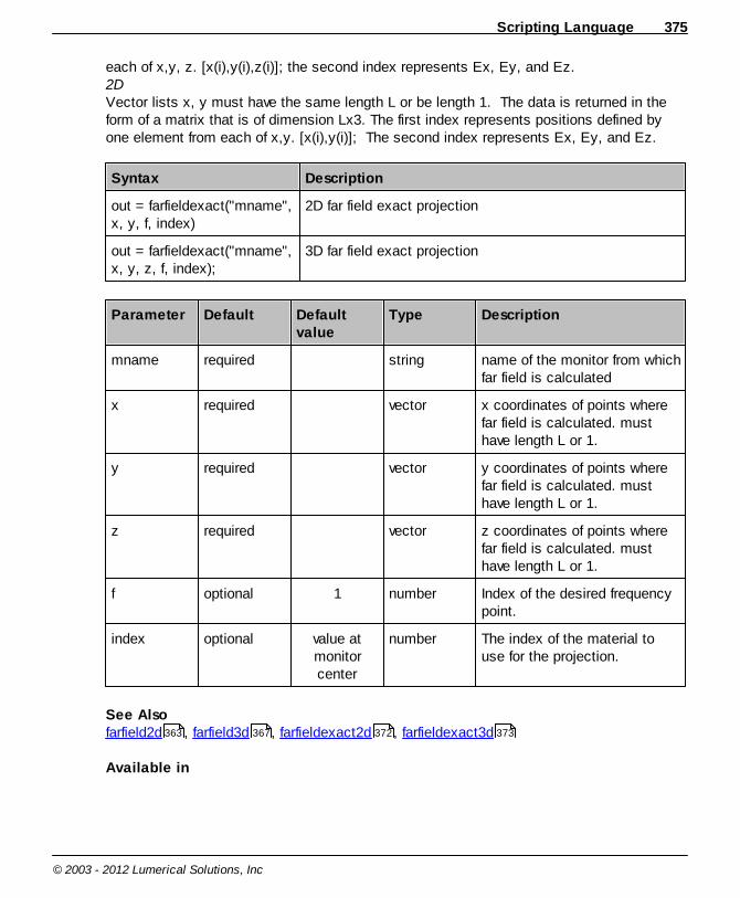
Scripting Language 375
© 2003 - 2012 Lumerical Solutions, Inc
each of x,y, z. [x(i),y(i),z(i)]; the second index represents Ex, Ey, and Ez. 2DVector lists x, y must have the same length L or be length 1. The data is returned in theform of a matrix that is of dimension Lx3. The first index represents positions defined byone element from each of x,y. [x(i),y(i)]; The second index represents Ex, Ey, and Ez.
Syntax Description
out = farfieldexact("mname",x, y, f, index)
2D far field exact projection
out = farfieldexact("mname",x, y, z, f, index);
3D far field exact projection
Parameter Default Defaultvalue
Type Description
mname required string name of the monitor from whichfar field is calculated
x required vector x coordinates of points wherefar field is calculated. musthave length L or 1.
y required vector y coordinates of points wherefar field is calculated. musthave length L or 1.
z required vector z coordinates of points wherefar field is calculated. musthave length L or 1.
f optional 1 number Index of the desired frequencypoint.
index optional value atmonitorcenter
number The index of the material touse for the projection.
See Alsofarfield2d , farfield3d , farfieldexact2d , farfieldexact3d
Available in
363 367 372 373
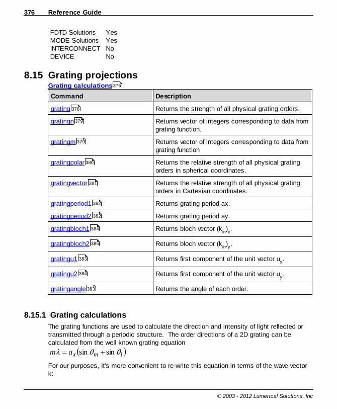
Reference Guide376
© 2003 - 2012 Lumerical Solutions, Inc
FDTD SolutionsMODE SolutionsINTERCONNECTDEVICE
YesYesNoNo
8.15 Grating projectionsGrating calculations
Command Description
grating Returns the strength of all physical grating orders.
gratingn Returns vector of integers corresponding to data fromgrating function.
gratingm Returns vector of integers corresponding to data fromgrating function
gratingpolar Returns the relative strength of all physical gratingorders in spherical coordinates.
gratingvector Returns the relative strength of all physical gratingorders in Cartesian coordinates.
gratingperiod1 Returns grating period ax.
gratingperiod2 Returns grating period ay.
gratingbloch1 Returns bloch vector (kin)x.
gratingbloch2 Returns bloch vector (kin)y.
gratingu1 Returns first component of the unit vector ux.
gratingu2 Returns first component of the unit vector uy.
gratingangle Returns the angle of each order.
8.15.1 Grating calculations
The grating functions are used to calculate the direction and intensity of light reflected ortransmitted through a periodic structure. The order directions of a 2D grating can becalculated from the well known grating equation
imxam sinsin
For our purposes, it's more convenient to re-write this equation in terms of the wave vectork:
376
378
379
379
380
381
382
382
384
385
383
384
383

Scripting Language 377
© 2003 - 2012 Lumerical Solutions, Inc
xxinxm
amkk
2)()(
In 3D, these equations become:
yyinymn
xxinxmn
amkk
ankk
2)()(
2)()(
,
,
where ax and a
y are the grating
periods in the x and y directionsrespectively and (n,m) are anyintegers where the condition
omn indexkk /2|| ,
is satisfied.
It's important to remember that the grating order directions are defined entirely by thedevice period, the source wavelength and angle of incidence, and the background refractiveindex. The grating order directions can be calculated without running a simulation, howeverthe simulation must first be meshed in order to obtain necessary information such as thedimensions and period of the structure. The functions gratingn, gratingm,
gratingu1, gratingu2 and gratingangle can be used to calculate the direction of
each order.
After running a simulation the grating commands can be used to calculate the fraction of
power that is scattered in each direction. The grating function uses a technique similar to afar field projection to calculate what fraction of near field power propagates in each gratingorder direction. To get polarization and phase information, use gratingpolar and
gratingvector.
Coordinate SystemsThe grating projections use the direction cosine coordinate system to specify far fieldpositions. Direction cosine units provide a convenient way to specify locations on ahemispherical surface, which is how the grating data is returned. Also, when calculatingvector field data (to obtain polarization information), you can choose to return the fieldsusing cartesian or spherical coordinates. For more information, please see the Coordinatesystems page.
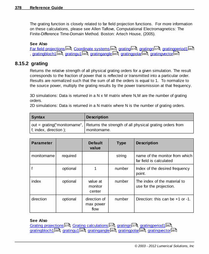
Reference Guide378
© 2003 - 2012 Lumerical Solutions, Inc
The grating function is closely related to far field projection functions. For more informationon these calculations, please see Allen Taflove, Computational Electromagnetics: TheFinite-Difference Time-Domain Method. Boston: Artech House, (2005).
See AlsoFar field projections , Coordinate systems , grating , gratingn , gratingperiod1, gratingbloch1 , gratingu1 , gratingangle , gratingpolar , gratingvector
8.15.2 grating
Returns the relative strength of all physical grating orders for a given simulation. The resultcorresponds to the fraction of power that is reflected or transmitted into a particular order. Results are normalized such that the sum of all the orders is equal to 1. To normalize tothe source power, multiply the grating results by the power transmission at that frequency.
3D simulations: Data is returned in a N x M matrix where N,M are the number of gratingorders.2D simulations: Data is returned in a N matrix where N is the number of grating orders.
Syntax Description
out = grating("monitorname",f, index, direction );
Returns the strength of all physical grating orders frommonitorname.
Parameter Defaultvalue
Type Description
monitorname required string name of the monitor from whichfar field is calculated
f optional 1 number Index of the desired frequencypoint.
index optional value atmonitorcenter
number The index of the material touse for the projection.
direction optional direction ofmax power
flow
number Direction: this can be +1 or -1.
See AlsoGrating projections , Grating calculations , gratingn , gratingperiod1 ,gratingbloch1 , gratingu1 , gratingangle , gratingpolar , gratingvector
359 361 378 379 382
384 383 383 380 381
376 376 379 382
384 383 383 380 381

Scripting Language 379
© 2003 - 2012 Lumerical Solutions, Inc
Available in
FDTD SolutionsMODE SolutionsINTERCONNECTDEVICE
YesYesNoNo
8.15.3 gratingn
Returns the vector of integers, n, corresponding to the values returned by grating. See theGrating calculation page for more information.
Syntax Description
out = gratingn( "monitorname",...);
Same arguments as grating function.
See AlsoGrating projections , Grating calculations , grating , gratingm
Available in
FDTD SolutionsMODE SolutionsINTERCONNECTDEVICE
YesYesNoNo
8.15.4 gratingm
Returns the vector of integers, m, corresponding to the values returned by grating. Onlyused in 3D simulations. See the Grating calculation page for more information.
Syntax Description
out = gratingm( "monitorname",...);
Same arguments as grating function.
See AlsoGrating projections , Grating calculations , grating , gratingn
Available in
376 376 378 379
376 376 378 379
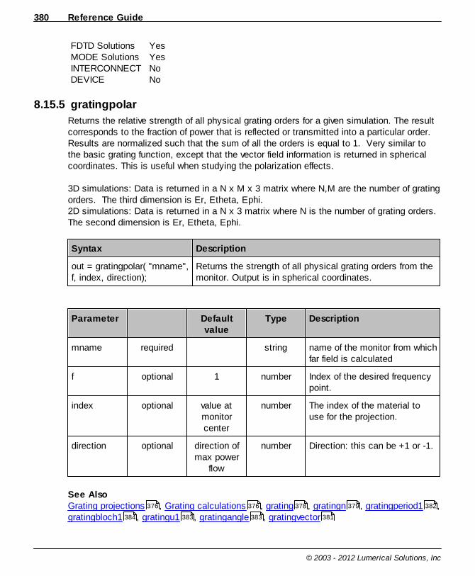
Reference Guide380
© 2003 - 2012 Lumerical Solutions, Inc
FDTD SolutionsMODE SolutionsINTERCONNECTDEVICE
YesYesNoNo
8.15.5 gratingpolar
Returns the relative strength of all physical grating orders for a given simulation. The resultcorresponds to the fraction of power that is reflected or transmitted into a particular order. Results are normalized such that the sum of all the orders is equal to 1. Very similar tothe basic grating function, except that the vector field information is returned in sphericalcoordinates. This is useful when studying the polarization effects.
3D simulations: Data is returned in a N x M x 3 matrix where N,M are the number of gratingorders. The third dimension is Er, Etheta, Ephi.2D simulations: Data is returned in a N x 3 matrix where N is the number of grating orders.The second dimension is Er, Etheta, Ephi.
Syntax Description
out = gratingpolar( "mname",f, index, direction);
Returns the strength of all physical grating orders from themonitor. Output is in spherical coordinates.
Parameter Defaultvalue
Type Description
mname required string name of the monitor from whichfar field is calculated
f optional 1 number Index of the desired frequencypoint.
index optional value atmonitorcenter
number The index of the material touse for the projection.
direction optional direction ofmax power
flow
number Direction: this can be +1 or -1.
See AlsoGrating projections , Grating calculations , grating , gratingn , gratingperiod1 ,gratingbloch1 , gratingu1 , gratingangle , gratingvector
376 376 378 379 382
384 383 383 381
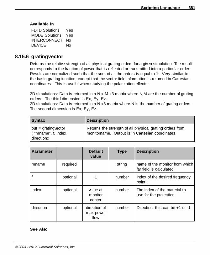
Scripting Language 381
© 2003 - 2012 Lumerical Solutions, Inc
Available in
FDTD SolutionsMODE SolutionsINTERCONNECTDEVICE
YesYesNoNo
8.15.6 gratingvector
Returns the relative strength of all physical grating orders for a given simulation. The resultcorresponds to the fraction of power that is reflected or transmitted into a particular order. Results are normalized such that the sum of all the orders is equal to 1. Very similar tothe basic grating function, except that the vector field information is returned in Cartesiancoordinates. This is useful when studying the polarization effects.
3D simulations: Data is returned in a N x M x3 matrix where N,M are the number of gratingorders. The third dimension is Ex, Ey, Ez.2D simulations: Data is returned in a N x3 matrix where N is the number of grating orders. The second dimension is Ex, Ey, Ez.
Syntax Description
out = gratingvector( "mname", f, index,direction);
Returns the strength of all physical grating orders frommonitorname. Output is in Cartesian coordinates.
Parameter Defaultvalue
Type Description
mname required string name of the monitor from whichfar field is calculated
f optional 1 number Index of the desired frequencypoint.
index optional value atmonitorcenter
number The index of the material touse for the projection.
direction optional direction ofmax power
flow
number Direction: this can be +1 or -1.
See Also
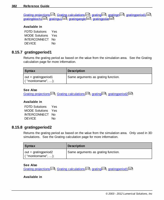
Reference Guide382
© 2003 - 2012 Lumerical Solutions, Inc
Grating projections , Grating calculations , grating , gratingn , gratingperiod1 ,gratingbloch1 , gratingu1 , gratingangle , gratingpolar
Available in
FDTD SolutionsMODE SolutionsINTERCONNECTDEVICE
YesYesNoNo
8.15.7 gratingperiod1
Returns the grating period ax based on the value from the simulation area. See the Gratingcalculation page for more information.
Syntax Description
out = gratingperiod1( "monitorname", ...);
Same arguments as grating function.
See AlsoGrating projections , Grating calculations , grating , gratingperiod2
Available in
FDTD SolutionsMODE SolutionsINTERCONNECTDEVICE
YesYesNoNo
8.15.8 gratingperiod2
Returns the grating period ax based on the value from the simulation area. Only used in 3Dsimulations. See the Grating calculation page for more information.
Syntax Description
out = gratingperiod2( "monitorname", ...);
Same arguments as grating function.
See AlsoGrating projections , Grating calculations , grating , gratingperiod1
Available in
376 376 378 379 382
384 383 383 380
376 376 378 382
376 376 378 382

Scripting Language 383
© 2003 - 2012 Lumerical Solutions, Inc
FDTD SolutionsMODE SolutionsINTERCONNECTDEVICE
YesYesNoNo
8.15.9 gratingangle
Returns the angle of each order corresponding to the values returned by grating, in degrees.Only available for 2d simulations. See the Grating calculation page for more information.
Syntax Description
out = gratingangle( "monitorname", ...);
Same arguments as grating function.
See AlsoGrating projections , Grating calculations , grating
Available in
FDTD SolutionsMODE SolutionsINTERCONNECTDEVICE
YesYesNoNo
8.15.10 gratingu1
Returns first component of the unit vector (ux) corresponding to the values returned by
grating. See the Grating calculation page for more information.
Syntax Description
out = gratingu1( "monitorname", ...);
Same arguments as grating function.
See AlsoGrating projections , Grating calculations , grating , gratingu2
Available in
FDTD SolutionsMODE SolutionsINTERCONNECTDEVICE
YesYesNoNo
376 376 378
376 376 378 384

Reference Guide384
© 2003 - 2012 Lumerical Solutions, Inc
8.15.11 gratingu2
Returns first component of the unit vector (uy) corresponding to the values returned by
grating. Only used in 3D simulations. See the Grating calculation page for moreinformation.
Syntax Description
out = gratingu2( "monitorname", ...);
Same arguments as grating function.
See AlsoGrating projections , Grating calculations , grating , gratingu1
Available in
FDTD SolutionsMODE SolutionsINTERCONNECTDEVICE
YesYesNoNo
8.15.12 gratingbloch1
Returns the value of the bloch vector (kin)x used for the calculation, based on the value for
the simulation area. See the Grating calculation page for more information.
Syntax Description
out = gratingbloch1( "monitorname", ...);
Same arguments as grating function.
See AlsoGrating projections , Grating calculations , grating , gratingbloch2
Available in
FDTD SolutionsMODE SolutionsINTERCONNECTDEVICE
YesYesNoNo
376 376 378 383
376 376 378 385

Scripting Language 385
© 2003 - 2012 Lumerical Solutions, Inc
8.15.13 gratingbloch2
Returns the value of the bloch vector (kin)y used for the calculation, based on the value for
the simulation area. Only used in 3D simulations. See the Grating calculation page formore information.
Syntax Description
out = gratingbloch2( "monitorname", ...);
Same arguments as grating function.
See AlsoGrating projections , Grating calculations , grating , gratingbloch1
Available in
FDTD SolutionsMODE SolutionsINTERCONNECTDEVICE
YesYesNoNo
8.16 Material databaseThe following commands are used to add or copy materials in the material database, aswell as to set any material property and verify the resulting complex index of a givenmaterial at any frequency. (The permittivity can be easily obtained by squaring the index.)Please see the chapter on the material database to understand the usage of thesecommands.
Command Description
addmaterial Adds a new material into the material database.
copymaterial Copies an existing material in the material database
setmaterial Sets any property of an existing material in thematerial database.
getmaterial Returns properties of a material in the materialdatabase.
getindex Returns the complex index of a material.
getfdtdindex Returns the material index as it will be in an actualFDTD simulation.
getmodeindex Returns the material index as it will be in an actual
376 376 378 384
386
386
387
387
388
388
389

Reference Guide386
© 2003 - 2012 Lumerical Solutions, Inc
MODE simulation.
getnumericalpermittivity An advanced function that returns permittivity, takinginto account the effect of finite size of dt in an FDTDsimulation.
8.16.1 addmaterial
Adds a new material to the material database.
Syntax Description
?addmaterial; Displays all types of materials that can be added into thematerial database.
out = addmaterial("materialtype");
Adds a new material and returns the name of the newmaterial. The argument "materialtype" is has to matchcorrect string exactly.
See AlsoMaterial database , setmaterial , getindex , getfdtdindex
Available in
FDTD SolutionsMODE SolutionsINTERCONNECTDEVICE
YesYesNoYes
8.16.2 copymaterial
Makes a copy of a material in the material database.
Syntax Description
out = copymaterial("materialname");
Creates a copy of the material "materialname". The newname is returned.
See AlsoMaterial database , setmaterial , getindex , getfdtdindex
Available in
390
385 387 388 388
385 387 388 388
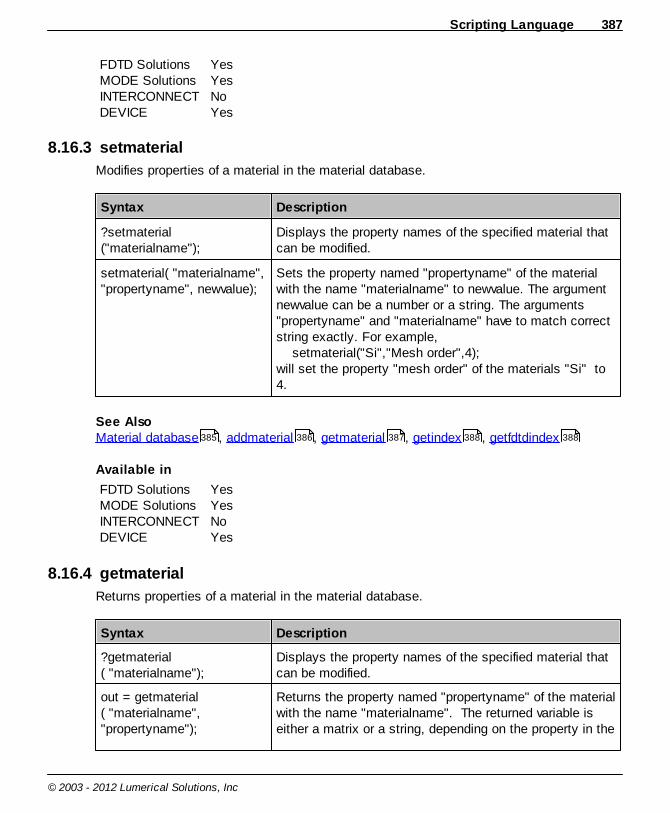
Scripting Language 387
© 2003 - 2012 Lumerical Solutions, Inc
FDTD SolutionsMODE SolutionsINTERCONNECTDEVICE
YesYesNoYes
8.16.3 setmaterial
Modifies properties of a material in the material database.
Syntax Description
?setmaterial("materialname");
Displays the property names of the specified material thatcan be modified.
setmaterial( "materialname","propertyname", newvalue);
Sets the property named "propertyname" of the materialwith the name "materialname" to newvalue. The argumentnewvalue can be a number or a string. The arguments"propertyname" and "materialname" have to match correctstring exactly. For example, setmaterial("Si","Mesh order",4);will set the property "mesh order" of the materials "Si" to4.
See AlsoMaterial database , addmaterial , getmaterial , getindex , getfdtdindex
Available in
FDTD SolutionsMODE SolutionsINTERCONNECTDEVICE
YesYesNoYes
8.16.4 getmaterial
Returns properties of a material in the material database.
Syntax Description
?getmaterial( "materialname");
Displays the property names of the specified material thatcan be modified.
out = getmaterial( "materialname","propertyname");
Returns the property named "propertyname" of the materialwith the name "materialname". The returned variable iseither a matrix or a string, depending on the property in the
385 386 387 388 388
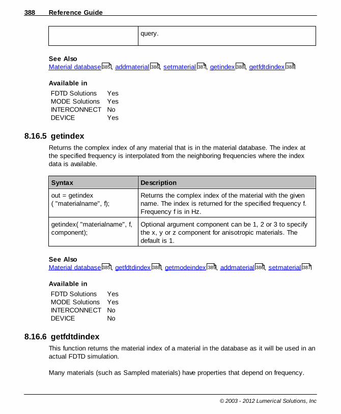
Reference Guide388
© 2003 - 2012 Lumerical Solutions, Inc
query.
See AlsoMaterial database , addmaterial , setmaterial , getindex , getfdtdindex
Available in
FDTD SolutionsMODE SolutionsINTERCONNECTDEVICE
YesYesNoYes
8.16.5 getindex
Returns the complex index of any material that is in the material database. The index atthe specified frequency is interpolated from the neighboring frequencies where the indexdata is available.
Syntax Description
out = getindex( "materialname", f);
Returns the complex index of the material with the givenname. The index is returned for the specified frequency f. Frequency f is in Hz.
getindex( "materialname", f,component);
Optional argument component can be 1, 2 or 3 to specifythe x, y or z component for anisotropic materials. Thedefault is 1.
See AlsoMaterial database , getfdtdindex , getmodeindex , addmaterial , setmaterial
Available in
FDTD SolutionsMODE SolutionsINTERCONNECTDEVICE
YesYesNoNo
8.16.6 getfdtdindex
This function returns the material index of a material in the database as it will be used in anactual FDTD simulation.
Many materials (such as Sampled materials) have properties that depend on frequency.
385 386 387 388 388
385 388 389 386 387
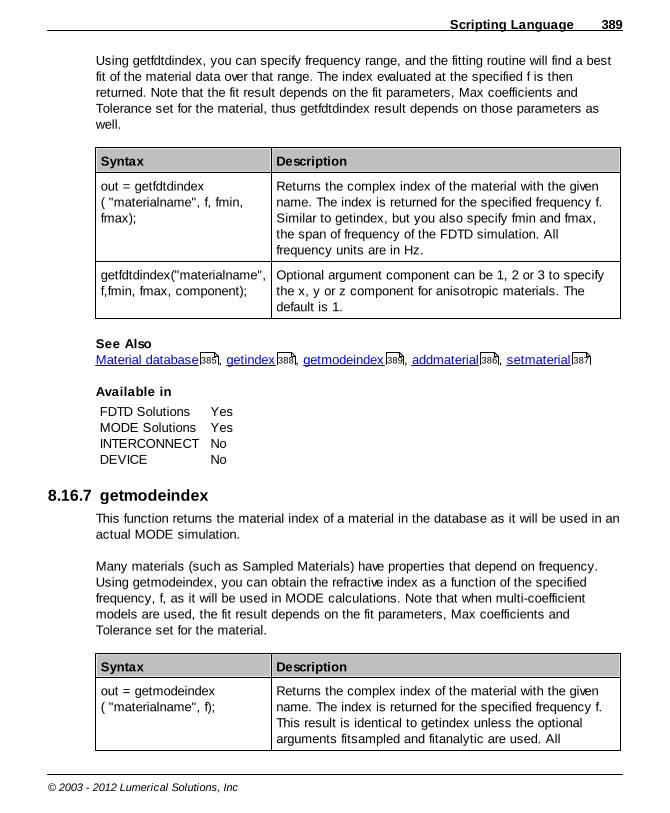
Scripting Language 389
© 2003 - 2012 Lumerical Solutions, Inc
Using getfdtdindex, you can specify frequency range, and the fitting routine will find a bestfit of the material data over that range. The index evaluated at the specified f is thenreturned. Note that the fit result depends on the fit parameters, Max coefficients andTolerance set for the material, thus getfdtdindex result depends on those parameters aswell.
Syntax Description
out = getfdtdindex( "materialname", f, fmin,fmax);
Returns the complex index of the material with the givenname. The index is returned for the specified frequency f.Similar to getindex, but you also specify fmin and fmax,the span of frequency of the FDTD simulation. Allfrequency units are in Hz.
getfdtdindex("materialname",f,fmin, fmax, component);
Optional argument component can be 1, 2 or 3 to specifythe x, y or z component for anisotropic materials. Thedefault is 1.
See AlsoMaterial database , getindex , getmodeindex , addmaterial , setmaterial
Available in
FDTD SolutionsMODE SolutionsINTERCONNECTDEVICE
YesYesNoNo
8.16.7 getmodeindex
This function returns the material index of a material in the database as it will be used in anactual MODE simulation.
Many materials (such as Sampled Materials) have properties that depend on frequency.Using getmodeindex, you can obtain the refractive index as a function of the specifiedfrequency, f, as it will be used in MODE calculations. Note that when multi-coefficientmodels are used, the fit result depends on the fit parameters, Max coefficients andTolerance set for the material.
Syntax Description
out = getmodeindex( "materialname", f);
Returns the complex index of the material with the givenname. The index is returned for the specified frequency f.This result is identical to getindex unless the optionalarguments fitsampled and fitanalytic are used. All
385 388 389 386 387
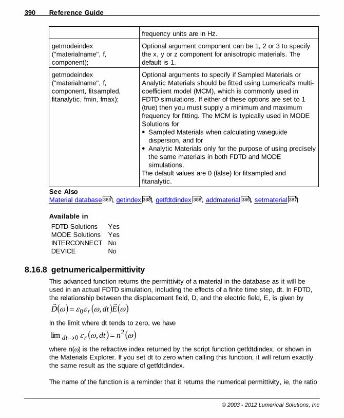
Reference Guide390
© 2003 - 2012 Lumerical Solutions, Inc
frequency units are in Hz.
getmodeindex("materialname", f,component);
Optional argument component can be 1, 2 or 3 to specifythe x, y or z component for anisotropic materials. Thedefault is 1.
getmodeindex("materialname", f,component, fitsampled,fitanalytic, fmin, fmax);
Optional arguments to specify if Sampled Materials orAnalytic Materials should be fitted using Lumerical's multi-coefficient model (MCM), which is commonly used inFDTD simulations. If either of these options are set to 1(true) then you must supply a minimum and maximumfrequency for fitting. The MCM is typically used in MODESolutions for
Sampled Materials when calculating waveguidedispersion, and forAnalytic Materials only for the purpose of using preciselythe same materials in both FDTD and MODEsimulations.
The default values are 0 (false) for fitsampled andfitanalytic.
See AlsoMaterial database , getindex , getfdtdindex , addmaterial , setmaterial
Available in
FDTD SolutionsMODE SolutionsINTERCONNECTDEVICE
YesYesNoNo
8.16.8 getnumericalpermittivity
This advanced function returns the permittivity of a material in the database as it will beused in an actual FDTD simulation, including the effects of a finite time step, dt. In FDTD,the relationship between the displacement field, D, and the electric field, E, is given by
EdtD r ,0
In the limit where dt tends to zero, we have
20 ,lim ndtrdt
where n( ) is the refractive index returned by the script function getfdtdindex, or shown inthe Materials Explorer. If you set dt to zero when calling this function, it will return exactlythe same result as the square of getfdtdindex.
The name of the function is a reminder that it returns the numerical permittivity, ie, the ratio
385 388 388 386 387

Scripting Language 391
© 2003 - 2012 Lumerical Solutions, Inc
of D and E, which is different from the refractive index, ie the ratio of the speed of light in avacuum to the phase velocity of light in the medium. To understand the relationshipbetween the them, we must consider the full, numerical dispersion relation between andk which is given by
2222
2sin
1
2sin
1
2sin
1
2sin
1,
dzk
dz
dyk
dy
dxk
dx
dt
cdtdt zyx
r
In the limit where dt, dx, dt and dz tend to zero, it is easy to show that we have theexpected result
)()0,( n
ck
dt
ck
r
The spatial FDTD mesh and time step are generally chosen to obtain a desired level ofsimulation accuracy, essentially by ensuring that the arguments of the sine functions aresufficiently small that sin(x)~x and that the simulation is stable. For some materials, it maybe desired to further reduce the value of the time step, dt, without modifying the spatialFDTD mesh, in order to obtain a higher level of accuracy for
r( ,dt). This script function
makes it possible to calculate, in advance, the value of dt required to obtain the desiredaccuracy for the permittivity.
Syntax Description
out =getnumericalpermittivity( "materialname", f, fmin,fmax, dt);
Returns the complex permittivity of the material with thegiven name. The permittivity is returned for the specifiedfrequency f. This is similar to getfdtdindex except for theadditional parameter dt. All frequency units are in Hz.
getnumericalpermittivity("materialname", f,fmin,fmax, dt, component);
Optional argument component can be 1, 2 or 3 to specifythe x, y or z component for anisotropic materials. Thedefault is 1.
See AlsoMaterial database , getindex , addmaterial , setmaterial , getfdtdindex
Available in
FDTD SolutionsMODE SolutionsINTERCONNECTDEVICE
YesYesNoNo
385 388 386 387 388
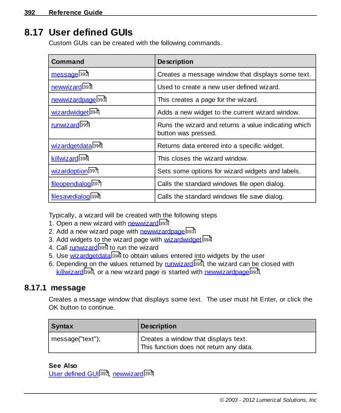
Reference Guide392
© 2003 - 2012 Lumerical Solutions, Inc
8.17 User defined GUIsCustom GUIs can be created with the following commands.
Command Description
message Creates a message window that displays some text.
newwizard Used to create a new user defined wizard.
newwizardpage This creates a page for the wizard.
wizardwidget Adds a new widget to the current wizard window.
runwizard Runs the wizard and returns a value indicating whichbutton was pressed.
wizardgetdata Returns data entered into a specific widget.
killwizard This closes the wizard window.
wizardoption Sets some options for wizard widgets and labels.
fileopendialog Calls the standard windows file open dialog.
filesavedialog Calls the standard windows file save dialog.
Typically, a wizard will be created with the following steps1. Open a new wizard with newwizard2. Add a new wizard page with newwizardpage3. Add widgets to the wizard page with wizardwidget4. Call runwizard to run the wizard5. Use wizardgetdata to obtain values entered into widgets by the user6. Depending on the values returned by runwizard , the wizard can be closed with
killwizard , or a new wizard page is started with newwizardpage .
8.17.1 message
Creates a message window that displays some text. The user must hit Enter, or click theOK button to continue.
Syntax Description
message("text"); Creates a window that displays text. This function does not return any data.
See AlsoUser defined GUI , newwizard
392
393
393
394
395
396
396
397
397
398
393
393
394
395
396
395
396 393
392 393
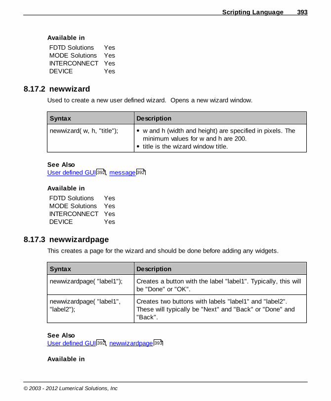
Scripting Language 393
© 2003 - 2012 Lumerical Solutions, Inc
Available in
FDTD SolutionsMODE SolutionsINTERCONNECTDEVICE
YesYesYesYes
8.17.2 newwizard
Used to create a new user defined wizard. Opens a new wizard window.
Syntax Description
newwizard( w, h, "title"); w and h (width and height) are specified in pixels. Theminimum values for w and h are 200. title is the wizard window title.
See AlsoUser defined GUI , message
Available in
FDTD SolutionsMODE SolutionsINTERCONNECTDEVICE
YesYesYesYes
8.17.3 newwizardpage
This creates a page for the wizard and should be done before adding any widgets.
Syntax Description
newwizardpage( "label1"); Creates a button with the label "label1". Typically, this willbe "Done" or "OK".
newwizardpage( "label1","label2");
Creates two buttons with labels "label1" and "label2".These will typically be "Next" and "Back" or "Done" and"Back".
See AlsoUser defined GUI , newwizardpage
Available in
392 392
392 393

Reference Guide394
© 2003 - 2012 Lumerical Solutions, Inc
FDTD SolutionsMODE SolutionsINTERCONNECTDEVICE
YesYesYesYes
8.17.4 wizardwidget
Adds a new widget to the current wizard window. This command should only be done aftercreating a new wizard page with the command newwizard.
Syntax Description
wizardwidget( "type","name");
type can be"number" for a numeric input field"string" for a alphanumeric field"checkbox" for a checkbox"menu" for a pulldown menu field"label" to add a string label (wizardgetdata does notreturn information for labels)
name is a string used to give the input field, checkbox,menu item or label a name.
wizardwidget( "type", "label",defaultValue);
defaultValue provides a default value for numeric inputs,checkboxes, menu items or strings.
wizardwidget( "type", "label","choices", defaultValue);
If the "type" of widget is a "menu", then the menu choicesmust be provided. These choices should be separated bythe character "|". For example, to create a pulldown widgetwith the name "simulation type" and 3 choices"TE","TM","3D", with the default choice "3D", thecommand iswizardwidget("menu","simulation type","TE|TM|3D",3);
See AlsoUser defined GUI , newwizardpage
Available in
FDTD SolutionsMODE SolutionsINTERCONNECTDEVICE
YesYesYesYes
392 393
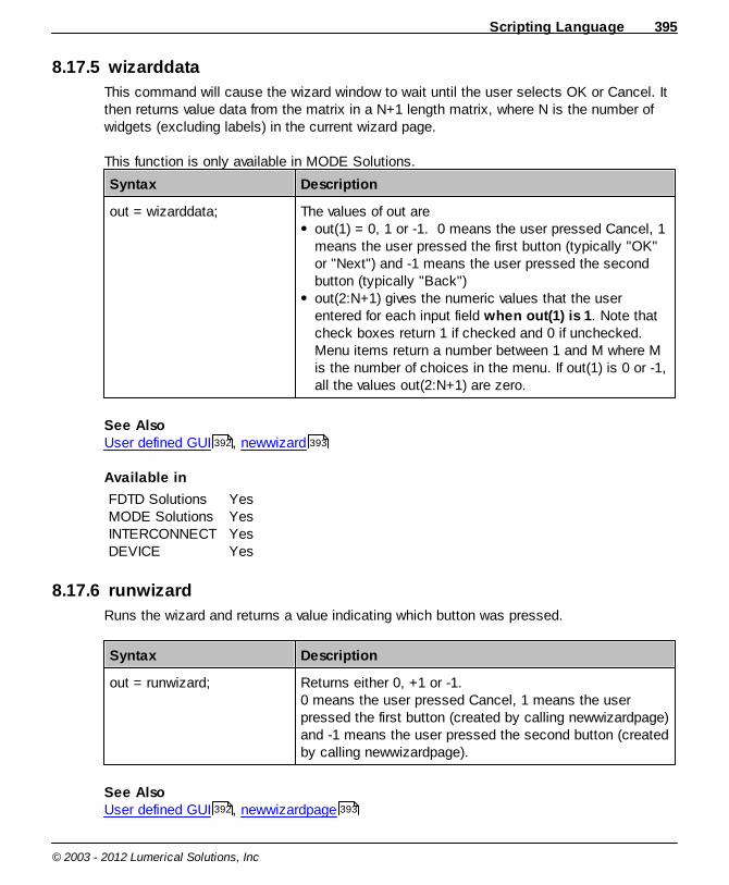
Scripting Language 395
© 2003 - 2012 Lumerical Solutions, Inc
8.17.5 wizarddata
This command will cause the wizard window to wait until the user selects OK or Cancel. Itthen returns value data from the matrix in a N+1 length matrix, where N is the number ofwidgets (excluding labels) in the current wizard page.
This function is only available in MODE Solutions.
Syntax Description
out = wizarddata; The values of out areout(1) = 0, 1 or -1. 0 means the user pressed Cancel, 1means the user pressed the first button (typically "OK"or "Next") and -1 means the user pressed the secondbutton (typically "Back")out(2:N+1) gives the numeric values that the userentered for each input field when out(1) is 1. Note thatcheck boxes return 1 if checked and 0 if unchecked.Menu items return a number between 1 and M where Mis the number of choices in the menu. If out(1) is 0 or -1,all the values out(2:N+1) are zero.
See Also User defined GUI , newwizard
Available in
FDTD SolutionsMODE SolutionsINTERCONNECTDEVICE
YesYesYesYes
8.17.6 runwizard
Runs the wizard and returns a value indicating which button was pressed.
Syntax Description
out = runwizard; Returns either 0, +1 or -1.0 means the user pressed Cancel, 1 means the userpressed the first button (created by calling newwizardpage)and -1 means the user pressed the second button (createdby calling newwizardpage).
See AlsoUser defined GUI , newwizardpage
392 393
392 393

Reference Guide396
© 2003 - 2012 Lumerical Solutions, Inc
Available in
FDTD SolutionsMODE SolutionsINTERCONNECTDEVICE
YesYesYesYes
8.17.7 wizardgetdata
Returns data entered into a specific widget.
This function is only available in MODE Solutions.
Syntax Description
out = wizardgetdata(N); Returns the value that the user entered into the Nth widget.Out will be a number or a string, depending on the type ofwidget.
See Also User defined GUI , newwizardpage
Available in
FDTD SolutionsMODE SolutionsINTERCONNECTDEVICE
YesYesYesYes
8.17.8 killwizard
This closes the wizard window. It should only be called after a wizard window has beencreated with the newwizard command.
Syntax Description
killwizard; This closes the wizard window.
See AlsoUser defined GUI , newwizardpage
Available in
392 393
392 393

Scripting Language 397
© 2003 - 2012 Lumerical Solutions, Inc
FDTD SolutionsMODE SolutionsINTERCONNECTDEVICE
YesYesYesYes
8.17.9 wizardoption
Sets some options for wizard widgets and labels.
Syntax Description
wizardoption ("optionname",setting);
The options are"fontsize" sets the font size to any value between 8 and40"fieldwidth" sets the width of each widget field to anyvalue between 20 and the full width of the wizard window."fieldheight" sets the height of each field to any valuebetween 8 and the full height of the wizard window."margin", sets size of the left margin to any valuebetween 0 and full width of the wizard window.
See AlsoUser defined GUI , newwizard
Available in
FDTD SolutionsMODE SolutionsINTERCONNECTDEVICE
YesYesYesYes
8.17.10 fileopendialog
Calls the standard windows file open dialog.
Syntax Description
out = fileopendialog; Brings up the open file dialog box and returns the path thatthe user selects.
out = fileopendialog(".ext"); Brings up the open file dialog box, displaying only files withthe extension .ext. Returns the path of the file that the userselects.
See Also
392 393
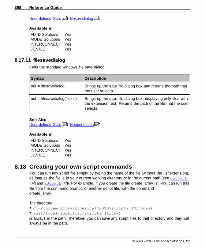
Reference Guide398
© 2003 - 2012 Lumerical Solutions, Inc
User defined GUIs , filesavedialog
Available in
FDTD SolutionsMODE SolutionsINTERCONNECTDEVICE
YesYesYesYes
8.17.11 filesavedialog
Calls the standard windows file save dialog.
Syntax Description
out = filesavedialog; Brings up the save file dialog box and returns the path thatthe user selects.
out = filesavedialog(".ext"); Brings up the save file dialog box, displaying only files withthe extension .ext. Returns the path of the file that the userselects.
See Also User defined GUIs , fileopendialog
Available in
FDTD SolutionsMODE SolutionsINTERCONNECTDEVICE
YesYesYesYes
8.18 Creating your own script commandsYou can run any script file simply by typing the name of the file (without the .lsf extension),as long as the file is in your current working directory or in the current path (see getpath
and addpath ). For example, if you create the file create_array.lsf, you can run this
file from the command prompt, or another script file, with the commandcreate_array;
The directoryC:\Program Files\Lumerical\FDTD\scripts (Windows)
/usr/local/lumerical/scripts (Linux)
is always in the path. Therefore, you can save any script files to that directory and they willalways be in the path.
392 398
392 397
170 170

Scripting Language 399
© 2003 - 2012 Lumerical Solutions, Inc
Script files must follow these formatting rules: Multiple commands are allowed on a single line.Blank lines, space and tabs will be ignored. Therefore you can format your script filesany way you choose. Each command should terminate with a semicolon. On any line, all characters after a # symbol are ignored. The last line in the script file must have a carriage return.
Finally, you can not define a variable or assign values to a variable that has the same nameas one of the script commands. For example, the following lines
sum = matrix(1,2);
angle = acos(pi/2);
are not valid statements and will return an error.
Note: All script files use a common variable space. As a consequence, variables defined in thescripts are global, and the script files have access to all variables defined in thesimulation project file.
This can lead to problems when two script files use the same variable names. Forexample, script_1.lsf (defined below) will print the value 10 to the command line
since script_2.lsf modified the variable i.script_1.lsfi=1;script_2;?i;
script_2.lsffor(i=1:10) { # do something}

Index 401
© 2003 - 2012 Lumerical Solutions, Inc
Index' 203
- 195
! 201, 202
!= 197
" 202
# 205
% 184
& 199, 200
* 194
/ 194
: 183
? 204
[] 184
196
| 200, 201
~ 202
+ 195
< 198
<= 198
= 183
== 196
> 199
>= 198
abs 213
absolute 213
access 190
acos 211
addanalysisgroup 265
addbulkgen 280
addcircle 266
addcustom 267
adddevice 278
adddiffusion 279
adddipole 273
addeigenmode 271
addfdtd 270
addgaussian 273
addgridattribute 280
addgroup 264
addimage 267
addimportdope 279
addimportedsource 275
addimportgen 280
addindex 275
addition 195
addjob 318
addmaterial 386
addmesh 272
addmode 272
addmodesource 273
addmovie 276
addobject 266
addpath 170
addplane 274
addpoly 268
addpower 277
addprofile 276
addpropagator 271
addpyramid 267
addrect 268
addring 269
addsphere 270
addstructuregroup 265
addsurface 270
addtfsf 274
addtime 276
addtogroup 290
addtriangle 269
adduserprop 291
almostequal 196
analysis 336
analysis group 104, 134
analysis tools 133
and 200
angle 214
Reference Guide402
© 2003 - 2012 Lumerical Solutions, Inc
anisotropic 121
apodization 108
arccos 211
arcsin 210
arctan 211, 212
array 183, 184, 190, 191
asap 91, 176, 177
asapexport 176
asapimport 177
asapload 176
asin 210
assign 190
assignment 183
atan 211
atan2 212
bestoverlap 340
boundary conditions 86
break 172
c 191
CAD layout 51
calculate modes 337
cd 163
ceil 246
centroid 240
changing CAD layout 64
clear 189
clearanalysis 352
cleardcard 353
clearjobs 319
clearsourcedata 307
closeall 261
comment 205
comparison 196
component 62
conductivity 117
conj 213
conjugate 213
copy 164, 290
copydcard 351
cos 209
cosine 209
coupling 338
cp 164
createbeam 277
cross 220
ctranspose 229
currentfilename 167
custom primitive 75
cwnorm 325
czt 238
data export 138
del 162
delete 285
deleteall 285
detail 74
Dielectric 117
dipolepower 328
dir 162, 163
division 194
dot 219
double quote 202
drude 117
edit 54
eig 220
eigenvalue 220
eigenvector 220
else 252
endl 204
eps0 191
equal 183
equal to 196
equation interpreter 114
escape 172
eval 230
exit 165
exp 216
exponential 216
exportfigure 260

Index 403
© 2003 - 2012 Lumerical Solutions, Inc
farfield2d 363
farfield2dintegrate 366
farfield3d 367
farfield3dintegrate 371
farfieldangle 365
farfieldexact 374
farfieldexact2d 372
farfieldexact3d 373
farfieldfilter 362
farfieldpolar2d 365
farfieldpolar3d 369
farfieldspherical 370
farfieldux 369
farfielduy 370
farfieldvector2d 364
farfieldvector3d 368
feval 231
fft 233
fftk 236
fftw 235
filebasename 167
filedirectory 168
fileexists 166
fileextension 168
fileopendialog 397
filesavedialog 398
find 227
findmodes 337
findpeaks 228
findstring 232
finite 249
flip 222
floor 246
for 251
format 173
framerate 312
frequencysweep 338
gaussian 248
gds 178
gdsii 77, 178
geometry 74
get 294
getcommands 169
getdata 349
getelectric 353
getfdtdindex 388
getglobalmonitor 298
getglobalsource 298
getindex 388
getmagnetic 354
getmaterial 387
getmodeindex 389
getnamed 296
getnamednumber 297
getnumber 296
getnumericalpermittivity 390
getpath 170
getsolver 299
getsourceangle 323
getsweepdata 348
getview 311
graphics graphical rendering 74
grating 376, 378
gratingangle 383
gratingbloch1 384
gratingbloch2 385
gratingm 379
gratingn 379
gratingperiod1 382
gratingperiod2 382
gratingpolar 380
gratingu1 383
gratingu2 384
gratingvector 381
greater than 199
greater than or equal to 198
groupscope 284
havedata 351
Reference Guide404
© 2003 - 2012 Lumerical Solutions, Inc
haveproperty 299
if 252
imag 212
image 258
imaginary 212
import 77, 178
import object 70
importnk 302
importnk2 304
importsurface 300
importsurface2 301
inpoly 241
integrate 225
integrate2 226
integration 49
interp 224
interpolate 224, 225
interptri 224
inverse 237
invfft 237
Kerr nonlinear 117
killwizard 396
layoutmode 264
legend 257
length 217
less than 198
less than or equal to 198
library 62
linecross 245
lineintersect 244
linspace 185
ln 215
load 161, 173
loaddata 173
location 74
log 215
log10 215
loop 251
lorentz 117
ls 163
main 52
main title bar 52
material 74, 117
material database 116
material models 117
matlab 138, 179
matlabget 181
matlabput 181
matlabsave 179
matrix 185, 191, 221
max 218
Max coefficients 117
mesh 127, 336
mesh refinement region 83
meshgrid3dx 187
meshgrid3dy 188
meshgrid3dz 188
meshgrid4d 188
meshgridx 186
meshgridy 187
message 392
min 219
mod 246, 247
model 117
modulus 246
monitor 104
mouse mode 55
move 165, 289
moving windows 64
mu0 191
multiplication 194
multiply 221
mv 165
natural 215
negative 195
new2d 159
new3d 159
newmode 160

Index 405
© 2003 - 2012 Lumerical Solutions, Inc
newproject 158
newwizard 393
newwizardpage 393
nonorm 324
normal 248
normalization 37
not 197, 201, 202
num2str 229
object tree 60
Optimization 150
or 201
orbit 311
order 127
output 204
overlap 339
Particle Swarm Optimization 150
path 170, 171
pause 171
PEC 117
permeability 191
permittivity 191
permute 222
phase 214
pi 191
pinch 217
plasma 117
plot 253
plotxy 254
polar 255
polar2 256
polarimage 257
polyand 242
polyarea 239
polydiff 243
polygrow 241
polyintersect 240
polyor 242
polyxor 244
power 196
priorities 127
product 219, 220
propagate 341
PSO 150
pwd 164
quit 165
rand 248
randmatrix 186
random 248
randreset 248
readdata 175
real 212
redo 313
redraw 307
redrawmode 309
redrawoff 308
redrawon 308
replace 232
replacestring 233
reshape 223
rm 162
rotations 74
round 246, 247
run 169, 317
runanalysis 350
runjobs 318
running a simulation 132
runparallel 317
runsetup 295
runsweep 319
runwizard 395
sampled data 117
save 161, 174
savedata 174
savedcard 174
screen 204
script 169
scripting editor prompt command line 63
seed 248
Reference Guide406
© 2003 - 2012 Lumerical Solutions, Inc
select 287
selectall 285, 286
selectfigure 259
selectmode 337
selectpartial 287
Sellmeier 117
set 292
set analysis 335
setanalysis 335
setglobalmonitor 293
setglobalsource 294
setmaterial 387
setnamed 292
setplot 260
setsourcesignal 305
setview 310
shiftselect 288
shiftselectpartial 289
sign 247
simulation 58
simulation region 83
sin 209
sine 209
single quote 203
size 74, 216
solar 249
source 91
sourceintensity 333
sourceintensity_avg 333
sourceintensity_pavg 334
sourcenorm 325
sourcenorm2_avg 326
sourcenorm2_pavg 327
sourcepower 329
sourcepower_avg 330
sourcepower_pavg 331
spectral averaging 108
speed of light 191
spline 225
sqrt 215
square root 215
str2num 230
string to number 230
strings 202, 203
structure 70
structures group 70
substring 231
subtraction 195
sum 218
surface 80
surface object 80
switchtolayout 264
system 166
tan 210
tangent 210
Tolerance 117
toolbar 52
transmission 321
transmission_avg 322
transmission_pavg 323
transparency 74
transpose 228
undo 313
units 37
unselectall 286
unwrap 214
updatesourcemode 306
variables with spaces 184
view 57
view ports perspective 60
visualize 259
which 171
wizarddata 395
wizardgetdata 396
wizardoption 397
wizardwidget 394
workspace 189
write 175

Index 407
© 2003 - 2012 Lumerical Solutions, Inc
z-transform 238