feasibility study about the mapping and monitoring of
TRANSCRIPT

Systèmes
d’Information
à Référence
Spatiale
27 rue du Carrousel - Parc de la Cimaise – Immeuble I – 59650 VILLENEUVE D’ASCQ 03.20.72.53.64 - 03.20.98.05.78 - E-Mail : [email protected] - Site Internet : www.sirs-fr.com
S.A.S. au capital de 312.025 € - RCS LILLE 444 654 271 – APE 6311 Z - N° d’identification FR 07 444 654 271 - SIRET 444 654 271 00022
Feasibility study about the mapping and monitoring of green linear features
based on VHR satellites imagery
EEA/MDI/14/006
Document: GLF_Final_Report
Issue: 1.3
Date: 20/03/2015

GLF_Final_Report Issue: 1.3
Green Linear Features Study Page 1 / 52
Document Preparation and Release
Affiliation Name(s) Date Signature
Author SIRS Antoine Lefebvre 10/11/2014
Contributions SIRS Christophe Sannier 15/12/2014
Review SIRS Alexandre Pennec 17/02/2015
Approval SIRS Jean-Paul Gachelin 17/02/2015
Document Issue Record
Issue Date Author(s) Description of Change
1.0. 10/11/2014 Christophe Sannier First Issue
1.1 15/12/2014 Antoine Lefebvre Issue 1.1
1.2 16/02/2015 Antoine Lefebvre Issue 1.2
1.3 20/03/2015 Antoine Lefebvre Issue 1.3

GLF_Final_Report Issue: 1.3
Green Linear Features Study Page 2 / 52
Table of Contents
.................................................................................................................................................... 0
1. Introduction ........................................................................................................................ 8
2. Review of existing methodologies for extracting green linear elements from VHR imagery ....................................................................................................................................... 8
3. Description of image processing workflows ...................................................................... 9
3.1. Workflow description .................................................................................................. 9
3.2. Use of VHR imagery provided through the GMES data warehouse DWH_MG2b_CORE_03. ......................................................................................................... 9
Main input data .................................................................................................... 9
Other input data sources ................................................................................... 11
3.3. Development of methods for the detection of small green linear features from the VHR imagery. ........................................................................................................................ 11
GLF geometry ..................................................................................................... 11
Object and Pixel-based image analysis .............................................................. 11
Extraction of Image variables ............................................................................. 12
Image variable selection .................................................................................... 14
Automatic selection of training sample set ....................................................... 16
Detection of green linear features ..................................................................... 16
Enhanced thematic and geometric results with data fusion ............................. 17
3.4. Classification of small green linear features ............................................................. 18
Green Linear Features typology ......................................................................... 18
Suggested nomenclature: a compromise between feasibility and potential confusion between classes ............................................................................................... 21
Classification process ......................................................................................... 22
3.5. GLF monitoring and changes/trends conclusions about the repeatability of the exercise to achieve a long-term monitoring. ....................................................................... 25
GLF monitoring ................................................................................................... 25
Change detection ............................................................................................... 25
4. Information about achieved accuracies ........................................................................... 26
4.1. Validation strategy for the mapping of green linear features for the EEA39 ........... 26
Stratification and sample design ........................................................................ 26
Response Design ................................................................................................ 27
Thematic accuracy .............................................................................................. 27
4.2. GLF Binary mask extraction ....................................................................................... 27

GLF_Final_Report Issue: 1.3
Green Linear Features Study Page 3 / 52
4.3. GLF Binary Mask extraction based on LPIS ................................................................ 30
4.4. Classification of GLF Types ........................................................................................ 30
4.5. GLF update and Change detection ............................................................................ 34
GLF update ......................................................................................................... 34
Change detection ............................................................................................... 34
Change detection refinement and GLF layers enhancement methodology ...... 35
5. Conclusions & Recommendations.................................................................................... 38
5.1. Evaluation if the developed methods can be applied for the EEA 39 area ............... 38
5.2. Estimations about the effort and cost for mapping the entire EEA 39 area ............. 38
Technical aspects................................................................................................ 39
Management aspects ......................................................................................... 40
Costs ................................................................................................................... 41
5.3. Proposal for the integration of LPIS data in the workflow ........................................ 42
References ................................................................................................................................ 43
6. ANNEX 1: Comparison between GLF layer and HRL Tree Cover Density layer ................ 45
7. ANNEX 2 : contribution of national LPIS web services ..................................................... 50

GLF_Final_Report Issue: 1.3
Green Linear Features Study Page 4 / 52
List of Figures
Figure 1 - Workflow and intermediate steps ........................................................................... 10
Figure 2 - Example of image variables computed on one of the SPOT-5 images for the French test area with (a) the original SPOT 5 data, (b) NDVI, (c) granulometry, (d) GLCM, (e) wavelet, (f) Gabor filter ........................................................................................................................... 13
Figure 3 - Examples of contextual information provided by Open Street Map for a grass filter strip along a small stream (yellow doted line) ......................................................................... 13
Figure 4 – Example Feature rank computed with the different variable selection methods .. 15
Figure 5 - Automatic sampling and refinement with (a) GIO HR Layer Forest, (b) Elimination of large areas and (c) Spatial refinement & outlier removal ................................................... 16
Figure 6 - Classifications computed with different classifiers based on pixel and object approach and associated overal accuracy level for the detection of GLF ............................... 17
Figure 7 - Data fusion provides (a) a classification of GLF with an overall accuracy of 92% and (b) areas of conflicts between the selected classification outputs. ......................................... 18
Figure 8 – Possible confusion between Mid-height hedge and ditch in Spain (top) and )Romania (bottom) ................................................................................................................... 19
Figure 9 – High hedgerow clearly (left) and not-clearly (right) identified ............................... 19
Figure 10 - Example of tree alignment in Sweden ................................................................... 20
Figure 11 - Example of a stone wall in Spain ............................................................................ 21
Figure 12 - Discrimination of small (a) areal and (b) linear features using mathematical morphology .............................................................................................................................. 24
Figure 13 - Green Linear Features detected by automated approach according the Level 3 of the nomenclature ..................................................................................................................... 25
Figure 14 - Illustration of the use of image gradient for the omission errors stratum: the validation points out of the GLF binary mask are selected in the yellow areas ...................... 26
Figure 15 Subsets of GLF binary mask. From top to the bottom, Czech Republic site, France site, Romania site, Sweden site and Spain site, ....................................................................... 29
Figure 16 - GLF binary mask based on LPIS edges: in yellow, a 25m buffer around LPIS edges ; in blue, the GLF not include in the LPIS buffer ......................................................................... 30
Figure 17 - Subset of the nomenclature classification of the study sites (low vegetation in yellow, high-hedges in blue, broadleaf patches in green, patches >0.5ha in grey)................. 32
Figure 18- Example of change detection: appearance in blue, disappearance in yellow ....... 35
Figure 19. Summary of findings. .............................................................................................. 39

GLF_Final_Report Issue: 1.3
Green Linear Features Study Page 5 / 52
List of Tables
Table 1 - Contribution of the main Green Linear Features ........................................................ 8
Table 2 - Processing time of image variable ............................................................................ 14
Table 3 - Variable selection for the 5 study sites ..................................................................... 15
Table 4 Possible confusion between GLF classes based on CAPI (without ancillary data) ...... 21
Table 5 Feasibility of GLF classification based on CAPI (without ancillary data) ..................... 22
Table 6 - Suggested nomenclature for green linear features .................................................. 22
Table 7 - Accuracy assessment for GLF binary mask ................................................................ 27
Table 8 - Accuracy assessment using LPIS ................................................................................ 30
Table 9 - Error matrices for the nomenclature classification of each site for points correctly identified as GLF ....................................................................................................................... 33
Table 10 - Accuracy assessment for GLF monitoring ............................................................... 34
Table 11 - Efforts and costs estimation according to the available data source ..................... 41

GLF_Final_Report Issue: 1.3
Green Linear Features Study Page 6 / 52
List of Abbreviations
AOI Area Of Interest
ARCH Assessing Regional Habitat Change in Kent and Nord-Pas de Calais
ASP Agence de Services et de Paiements
CAP Common Agricultural Policy
CAPI Computer Assisted Photo Interpretation
CLC Corine Land Cover
COTS Commercial off The Shelf
CwRS Control with Remote Sensing
DN Digital Number
EEA European Environment Agency
EEA39 EEA’s 39 countries
FTY Forest TYpe
GAEC Good Agricultural and Environmental Conditions
GDAL Geospatial Data Abstraction Library
GIO GMES Initial Operations
GIO GMES Initial Operations
GIS Geographic Information System
GLCM Grey Level Coocurrence Matrix
GLE Green Linear Elements
GLF Green Linear Features
GMES Global Monitoring for Environment and Security
GRA GRAssland
HR High Resolution
HRL High Resolution Layer
LC / LU Land Cover / Land Use
LGV Ligne à Grande Vitesse
LPIS Land Parcel Identification
LUCAS Land Use/Cover Area frame statistical Survey
LUZ Large Urban Zone
MMU Minimum Mapping Unit
NDVI Normalized Difference Vegetation Index
OA Overall Accuracy
OBIA Object Based Image Analysis
OSM Open Street Map
OSM Open Street Map
OTB Orfeo ToolBox
QA Quality Assurance
QC Quality Control
QC Quality Control
RS Remote Sensing
SBS Sequential Backward Selection
SFS Structural Features Set
SIRS Systèmes d’Information à Référence Spatiale

GLF_Final_Report Issue: 1.3
Green Linear Features Study Page 7 / 52
SL Sealing Level
SVM Support Vector Machine
UA Urban Atlas
VHR Very High Resolution
VHSR Very High Spatial Resolution
WET WETland
GLF_Final_Report Issue: 1.3
Green Linear Features Study Page 8 / 52
1. Introduction
Green linear features (GLF), such as ditches, hedgerows, lines of trees and grass filter strips provide
numerous ecological and socio-cultural functions, which can be grouped in 4 main categories
Soil and water conservation: Specific features such as grass filter strips slow runoff from fields,
filtering pesticides and other potential pollutants before they reach surface waters.
Climate protection and adaptation: significant role in flood and landslides mitigation, carbon
storage and sequestration.
GLF support biological diversity by facilitating the free movement of certain species between
different habitats patches (Forman and Godron, 2008) thus providing important habitats and
ecosystem services (Van der Zanden et al., 2013).
Cultural identity: GLF compose and structure the rural landscape, they reflect the local
agricultural history and provide a large variety of traditional landscape trough Europe
(Jongman R., 1995) thus providing an important cultural value.
Table 1 summarizes these categories according to the contribution of the main types of GLF. It
highlights that a specific GLF cannot ensure all these functions on its own and the presence of all GLF
throughout the rural landscape is essential to maintain a balanced environment.
Table 1 - Contribution of the main Green Linear Features
Ecological functions Socio-cultural functions
Soil and water conservation
Climate protection/ adaptation
Biodiversity flora, fauna, habitats
Cultural identity, landscape aesthetics
Hedgerows + + +++ +++
Stone walls ++ + ++ +++
Green strips +++ ++ +++ +
trees/scrub patches ++ ++ +++ +++
Ditches +++ + +++ ++
2. Review of existing methodologies for extracting green linear
elements from VHR imagery
Among the scientific publications, several methods dealing with landscape feature mapping from
remote-sensing data have shown that satellite images or aerial photographs with high or very high
spatial resolution are suitable for automatic hedgerow mapping.
The most accurate method is certainly manual digitization from airborne photographs (Baudry et al.
2000; Department for Environment, Food and Rural Affair (DEFRA) 2007; Lotfi et al. 2010). Although
this approach is time- consuming and labour-intensive.
Considering automated approaches, two methodologies stand out: methodologies based on pixel and
on objects. Their performances are still under discussion and their advantages and drawbacks can be
contradictory depending on authors. It seems that the prevalence of a particular approach mostly
depend on the context of study and more particularly on the data available and the area to be
processed.

GLF_Final_Report Issue: 1.3
Green Linear Features Study Page 9 / 52
Object based approaches proved their efficiency for mapping complex landscape with VHR1 images.
The eCognition software was mostly used for segmenting the image (Vannier and Hubert-Moy, 2014;
Tansey et al., 2009). To be effective, it requires setting a number of parameters such as object size,
color homogeneity, shape, smoothness, and compactness. Moreover, it is based on a multi-resolution
segmentation approach for which, depending on the segmentation level, the landscape is represented
at three scales corresponding to tree, hedge, and field levels. Different spectral features and fuzzy
membership functions can be used to classify the resulting objects. However, the need for adjusting
individually many parameter values for multi-scale segmentation and classification for each image may
limit the general applicability of this method.
Pixel based approaches provide similar classification accuracies, and are less time-consuming than
object-based classifications (Duro et al., 2012). Pixel based approaches gain in efficiency when several
image variable are derived from the initial image. Texture features rely on a pixel neighbourhood
analysis and constitute an alternative to object-based approach. For example, Lennon et al. (2000)
used a fuzzy combination of a vegetation index, a linearity feature based on image gradient, and co-
occurrence texture features for data obtained from an airborne hyperspectral sensor. Fauvel et al.
(2013) used mathematical morphology to extract contextual information. In order to limit data
multiplication and test image variable performance, Aksoy et al. (2010) also showed the effectiveness
of a multi-feature selection strategy for hedgerows classification.
3. Description of image processing workflows
3.1. Workflow description
The image processing and classification methods for this project have been developed in consideration of both input data and geometric/thematic precision of deliveries. Existing SIRS automated image processing chains were adapted for the GLF production. In-house solutions are generally preferred to COTS software based processing chains such as eCognition, ERDAS or ENVI as it provides a higher degree of flexibility and the use of MatLab, Orfeo Toolbox (OTB), Open CV and GDAL libraries ensures that the latest development in terms of image processing and classification algorithms are available. The project was broken in 4 main steps:
Extraction of undifferentiated green linear features
Classification of green linear features
Change detection
Quality assurance and quality check
The workflow is presented in Figure 1. A detailed description of each step of the methodology is
provided in the following sections.
3.2. Use of VHR imagery provided through the GMES data warehouse DWH_MG2b_CORE_03.
Main input data
GLF map products for this study were developed based on the VHSR SPOT 5 imagery acquired as part of the DWH_MG2b_CORE_03 dataset of the GMES data warehouse that provides multi-spectral information at a fine scale. However, considering the potential application at pan-European level and based on our experience with the UA2012 and GIO HR Layers production, the acquisition time window

GLF_Final_Report Issue: 1.3
Green Linear Features Study Page 10 / 52
of the imagery is potentially widely spread. This is confirmed by the acquisition dates of the imagery for the selected test sites acquired at different times during the growing season. The main implication is that the classification methods developed cannot rely solely on spectral information. In this context, the project presents a number of technical challenges similar to that of the UA2012 and GIO HR Layers mainly in relation to data heterogeneity and scene complexity. SIRS already successfully overcome these challenges as part of the UA2012 and GIO HR Layers, developing robust and efficient automatic processing methods that have required minimal adaptation to fit the requirements of the GLF product. In addition, one of the main challenges of the study is the detection of significant changes in GLF. Therefore, to maximize the probability to detect changes, it was suggested at the project onset to use existing UA2006 data instead of the data suggested in the tender specifications which were only a few months apart. Of the three sites where more than one image is available, there is only just a few months between image acquisition dates and it is unlikely that changes in GLF will have taken place. Therefore, it was suggested that 2 sites (France and Romania) should be changed and one site slightly shifted (Spain) to take advantage of the available UA2006 imagery.
Figure 1 - Workflow and intermediate steps

GLF_Final_Report Issue: 1.3
Green Linear Features Study Page 11 / 52
Other input data sources
The following Copernicus/GMES core datasets were used as part of the production process to provide
means of automatically extract training data thus fostering the applicability of the method for the
EEA39 area :
GIO HR Layer Forest & Grassland: will be used as part of training of the automated classification
process, HRL Grassland will only be used if its quality is deemed sufficient.
Other GIO HR Layer Wetland and Permanent Water Bodies and associated support layers:
these data sets could complement the OSM dataset to support the automated classification
process
Initially, it was envisaged that the production would also require the following data sets:
LUCAS 2009-2012 point sampling of terrain photographs and LC/LU description: can be used
for accuracy assessment as an independent reference dataset, this dataset did not prove
useful for the purpose of this exercise over a small number of sites. It could nevertheless be
considered for an application over the EEA39 area
Land Parcel Identification System (LPIS): linear, areal and point green features can be extracted
to be part of training of the automated classification process. However, access to LPIS data is
still problematic for most countries. A simplified version of the LPIS was used in France to limit
commission errors
Open Street Map dataset (waterways, roads, railways layers): provided contextual information
purposes to support the automated classification process
3.3. Development of methods for the detection of small green linear features from the VHR imagery.
GLF geometry
GLF are defined as objects with a minimum length of 25 m (~10 pixels length) and a maximum width
of 10 m for linear elements, and a minimum of 500 m2 size (~10 pixels diameter) for small patches of
trees and scrub.
The product specifications do not include an upper limit for GLF patches. In fact, it is difficult to define
such a limit because GLF can be in the form of a network which can represent potentially large areas.
An upper limit for GLF patches can only be determined with reference to another standard areal LC/LU
dataset, i.e. the MMU of the areal dataset could determine the maximum size of isolated GLF patches.
For instance, in the case of the Riparian Zones project, the upper limit of GLF patches is the MMU of
the LC/LU dataset, i.e. 0.5 ha. However, this dataset is unlikely to be available over the whole of the
EEA39 and an alternative would be required. A possibility would be to use the HR layer FTY with a
MMU of 0.5 ha, but this would only be applicable to tree patches and not scrub patches. For scrub
patches, the use of HRL WET and GRA could also be investigated.
For this study, the HR layer FTY was not available over several test sites and CLC2006 was used as an
alternative to set an upper limit for GLF patches
Object and Pixel-based image analysis
The main difficulty when dealing with VHSR images comes from the internal variability of the
information for a single land-use. For instance, woody elements are represented by a high number of
heterogeneous pixel values hampering usual pixel-based techniques. Nevertheless, even though

GLF_Final_Report Issue: 1.3
Green Linear Features Study Page 12 / 52
object-based image analysis (OBIA) appears to be the most suitable approach to delineate GLF with
VHSR images; it can potentially represent some serious drawbacks related to the heterogeneous size
and shape of GLF objects and the difficulty to determine suitable segmentation parameters (Fauvel et
al., 2013). In addition, for very small object close to the resolution of the imagery, the segmentation
can lead to separate GLF or non-GLF objects to be merged together due to mixed pixel values. This
makes particularly difficult to define a suitable segmentation scale in different landscapes particularly
if it is to be applied for the EE39 area. Therefore, object level was not investigated in this feasibility
study.
Extraction of Image variables
Multispectral information and derivatives such as the NDVI are essential to discriminate landscape
elements but are not sufficient. GLF can be thin, sinuous, fragmented and easily confused with some
other neighboring vegetation features. An effective delineation requires advanced feature computing
able to discriminate objects that have similar spectral responses but different texture, shape and
context.
A large set of variables were computed and can be grouped according to their properties as follow:
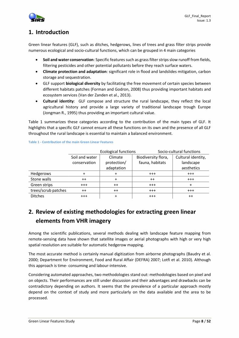
Granulometry by Different Morphology Profile (DMP): Mathematical morphology is the
analysis of the image structures and their distribution at different scale. It consists in
simplifying the image progressively though the preservation of bright elements (with closing
operators) or dark elements (opening operators). This technique can highlight specific shapes
in the image and is suitable for the detection of some GLF (Aksoy, 2010; Fauvel et al., 2013). It
removes image noise, which leads to enhancement of thin networks of hedges (Figure 2.c).
Texture / Structure: Texture and structure analysis consists in extracting information on the
spatial arrangement of pixels. This analysis can be applied at different scale, it is then
particularly useful to detect the treetop texture of wooded areas but also the structure of GLF
networks at a coarse scale. Amongst numerous existing techniques, the following are
particularly interesting for GLF delineation:
o Grey Level Co-occurrence Matrix: it is a widely used texture analysis technique in
remote sensing. It consists in the distribution analysis of co-occurring pixel values at a
given offset. Numerous indexes are derived from this matrix to extract texture
properties (Haralick, 1973). It can be considered an efficient technique for the
detection hedgerow (Figure 2.d), despite the fact it is time consuming and requires a
high level of parameterization,
o Wavelet: Signal decomposition techniques are used to provide a multi-resolution
representation of the original image in a series of components related to a specific
direction (Figure 2.e). Wavelet analysis applied to VHSR images showed their efficiency
for detecting textured objects (Lefebvre et al., 2011)
o Gabor filter: it is a linear filter used for edge detection. A bank of filter can be defined
by selected frequencies and orientations to extract specific structures in an image. This
technique was already successfully applied to detect hedgerows (Aksoy, 2010).
GLF_Final_Report Issue: 1.3
Green Linear Features Study Page 13 / 52
(a)
(b)
(c)
(d)
(e)
(f)
Figure 2 - Example of image variables computed on one of the SPOT-5 images for the French test area with (a) the original
SPOT 5 data, (b) NDVI, (c) granulometry, (d) GLCM, (e) wavelet, (f) Gabor filter
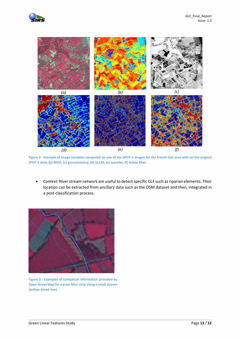
Context: River stream network are useful to detect specific GLF such as riparian elements. Their
location can be extracted from ancillary data such as the OSM dataset and then, integrated in
a post-classification process.
Figure 3 - Examples of contextual information provided by
Open Street Map for a grass filter strip along a small stream
(yellow doted line)

GLF_Final_Report Issue: 1.3
Green Linear Features Study Page 14 / 52
Production of the GLF/GLE layer over the EEA39 requires the processing of several thousands of VHR
images. Therefore, computation time can be a significant criterion that has to be evaluated in order to
estimate its feasibility. An average computation time to produce variables for a SPOT-5 image was
measured on a dedicated workstation (Xeon 8 cores, 32 Go RAM). Results presented in Table 2 show
that all variables except GLCM are fast to process and suitable for an application over the EEA39. GLCM
are particularly slow because their computations are based on a sliding window browsing the overall
image. The source code used to produce these variables is from the Orfeo Toolbox library, it used
parallel computing and is one of the fastest method available.
Table 2 - Processing time of image variable
Variable Duration Comments
Band 0 min Very fast NDVI 1 min Very fast
Gradient 5 min Fast Gabor 5 min Fast DMP 5 min Fast
GLCM 60 min Very slow
Image variable selection
The numerous image variables described in the previous section result in a high-dimensional image
feature set containing some redundant information. Consequently, the number of variables given as
input to a classifier can be reduced without a considerable loss of information. Such reduction
obviously leads to a sharp decrease in the processing time required by the classification process. In
addition, it may also provide an improvement in classification accuracy due to the Hughes effect
(Serpico and Bruzzone, 2001).
3 variable selection methods were tested:
- Fisher score is the ratio of the variance of the between classes to the variance of within classes.
This method is suitable when values have a normal distribution.
- Sequential Backward Selection (SBS) is an iterative algorithm that starts with all features and
shrinks down the feature set by, at each iteration, removing the single worst feature from the
set of features obtained in the previous iteration (Duda et al., 2000). The SBS has already been
successfully applied to remote sensing data (Serpico and Bruzzone, 2001) and it has been
showed that this method improved significantly the classification accuracy of GLF (Aksoy,
2010).
- Variable importance based on random forest models
These techniques provide a score to each variable that can be manually threshold. An example for the
French site shown in Figure 4 highlight the most relevant variables. The 3 methods bring out that the
Green band, the gradient (scale 2) and the DMP (scale 1 to 3) are the most important variable for the
extraction of the GLF.

GLF_Final_Report Issue: 1.3
Green Linear Features Study Page 15 / 52
Figure 4 – Example Feature rank computed with the different variable selection methods
This analysis was performed on all sites and selected variables were reported in Table 3. The number
of occurrence when a variable is selected provides an indication of the most relevant variables over
the EEA39. The main variables that should be used to extract GLF are mainly:
the input bands (especially the Red and Green), NDVI,
the DMP (scale 1, 2 and 3),
the GLCM features (especially correlation and Inverse Difference Moment)
Gabor filter (scale 2).
Table 3 - Variable selection for the 5 study sites
0
0,2
0,4
0,6
0,8
1
Variable importance (FR)
Fisher score Random Forest Sequential Backward Selection
GLF_Final_Report Issue: 1.3
Green Linear Features Study Page 16 / 52
Automatic selection of training sample set
To maximize the applicability of the method for the EEA39 area and foster economies of scale, the use of automated training sample set selection should be applied. Sampling of training or calibration data can be based on the GIO Forest HR Layer, LPIS and if considered of suitable accuracy HRL Grassland. Even if GIO HR Layers can be considered as coarse resolution compared with that of the GLF/GLE layer, it remains a suitable dataset to perform an automated sampling selection: the GIO Forest HR Layer is potentially available over the EEA39 territory, the thematic nomenclature can be used to define a part of the thematic resolution of the GLF. As a result, the use of GIO Forest HR Layer will request a low level of input from the operator (thus saving considerable time and effort). Changed areas and objects below the GIO HR Layer MMU can be represented by a small number of
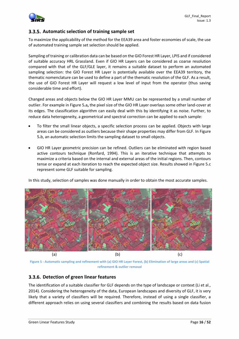
outlier. For example in Figure 5.a, the pixel size of the GIO HR Layer overlays some other land-cover at
its edges. The classification algorithm can easily deal with this by identifying it as noise. Further, to
reduce data heterogeneity, a geometrical and spectral correction can be applied to each sample:
To filter the small linear objects, a specific selection process can be applied. Objects with large areas can be considered as outliers because their shape properties may differ from GLF. In Figure 5.b, an automatic selection limits the sampling dataset to small objects.
GIO HR Layer geometric precision can be refined. Outliers can be eliminated with region based active contours technique (Ronfard, 1994). This is an iterative technique that attempts to maximize a criteria based on the internal and external areas of the initial regions. Then, contours tense or expand at each iteration to reach the expected object size. Results showed in Figure 5.c represent some GLF suitable for sampling.
In this study, selection of samples was done manually in order to obtain the most accurate samples.
(a) (b) (c)
Figure 5 - Automatic sampling and refinement with (a) GIO HR Layer Forest, (b) Elimination of large areas and (c) Spatial
refinement & outlier removal
Detection of green linear features
The identification of a suitable classifier for GLF depends on the type of landscape or context (Li et al.,
2014). Considering the heterogeneity of the data, European landscapes and diversity of GLF, it is very
likely that a variety of classifiers will be required. Therefore, instead of using a single classifier, a
different approach relies on using several classifiers and combining the results based on data fusion

GLF_Final_Report Issue: 1.3
Green Linear Features Study Page 17 / 52
techniques (section 3.3.7) to provide a single more robust and precise classification. This approach has
already been used as part of the GIO HRL and UA2012 production.
This step is supervised by a sample dataset as detailed in section 3.3.5. Classification models are then
automatically created during a calibration stage.
The following classification algorithms are likely to be included:
Maximum-Likelihood: Maximum-Likelihood Estimation is probably the most popular classifier
in remote sensing. It is based on the assumption that features associated with each class are
distributed according to a Gaussian distribution. Results are then easy to understand but can
lead to spurious results if the data is not normally distributed.
Support Vector Machine: SVM is an advanced classifier representing input data in a specific feature space within which each class is ‘easily’ separable. This method is particularly robust and has already proved its efficiency to classify GLF from VHSR images (Fauvel et al., 2007). The prime advantage of the SVM classification is that it has the benefits to require very few parameters.
Random Forest: Random Forest combines many decision trees to obtain better predictive
performance. Each decision tree is calibrated on a selection of random subset. It is considered
as a highly accurate classifier, which runs efficiently on large dataset. It can deal with outliers
effectively and provide relation between large image feature sets and thematic classes.
Neural Networks: Neural networks consist of a set of adaptive functions (neurons) able to
approximate a non-linear system. Neural networks algorithm is particularly suitable when a
large quantity of samples is available (Benediktsson et al., 1990).
Examples of classification outputs are presented in Figure 6.
Figure 6 - Classifications computed with different classifiers based on pixel and object approach and associated overal
accuracy level for the detection of GLF
Enhanced thematic and geometric results with data fusion
As described in the previous section, the idea is not to select a single classifier but to take advantages
on several classification algorithms to get an enhanced result that cannot be reached by any of them
independently. This is possible with data fusion techniques.
Maximum Likelihood Estimation
Neural Networks Random Forest Support Vector Machine
Pix
el b
ased
OA = 89%
OA = 67%
OA = 90%
OA = 90%
GLF_Final_Report Issue: 1.3
Green Linear Features Study Page 18 / 52
Amongst available data fusion techniques, Dempster-Shafer evidence theory provides relevant
advantages such as (i) modelling of the uncertainty and imprecision, (ii) the computation of conflict
between classifications and (iii) the possible introduction of a priori information (Bloch, 1996).
Dempster-Shafer evidence Theory has already showed its efficiency on numerous application such as
multisource multispectral images and was implemented for the GIO HRL and UA2012 production
(Lefebvre et al., 2013 ; Le Hegarat-Mascle, 1997 ; Lu et al., 2006).
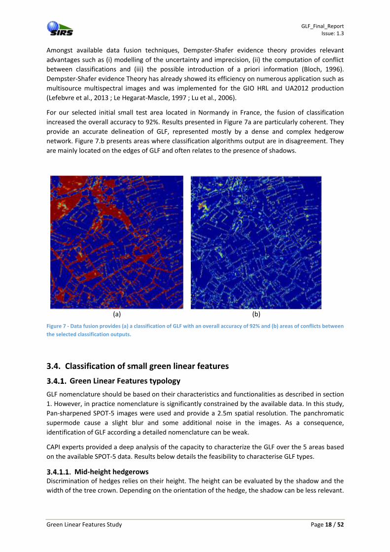
For our selected initial small test area located in Normandy in France, the fusion of classification
increased the overall accuracy to 92%. Results presented in Figure 7a are particularly coherent. They
provide an accurate delineation of GLF, represented mostly by a dense and complex hedgerow
network. Figure 7.b presents areas where classification algorithms output are in disagreement. They
are mainly located on the edges of GLF and often relates to the presence of shadows.
(a) (b)
Figure 7 - Data fusion provides (a) a classification of GLF with an overall accuracy of 92% and (b) areas of conflicts between
the selected classification outputs.
3.4. Classification of small green linear features
Green Linear Features typology
GLF nomenclature should be based on their characteristics and functionalities as described in section
1. However, in practice nomenclature is significantly constrained by the available data. In this study,
Pan-sharpened SPOT-5 images were used and provide a 2.5m spatial resolution. The panchromatic
supermode cause a slight blur and some additional noise in the images. As a consequence,
identification of GLF according a detailed nomenclature can be weak.
CAPI experts provided a deep analysis of the capacity to characterize the GLF over the 5 areas based
on the available SPOT-5 data. Results below details the feasibility to characterise GLF types.
Mid-height hedgerows Discrimination of hedges relies on their height. The height can be evaluated by the shadow and the
width of the tree crown. Depending on the orientation of the hedge, the shadow can be less relevant.

GLF_Final_Report Issue: 1.3
Green Linear Features Study Page 19 / 52
Mid-height hedges are also often confuse with ditches whatever the areas of interest (Figure 8 –
Possible confusion between Mid-height hedge and ditch in Spain (top) and )Romania (bottom)).
SPOT-5 image Google Earth Google Street View
SPOT-5 image Google Earth Google Street View
Figure 8 – Possible confusion between Mid-height hedge and ditch in Spain (top) and )Romania (bottom)
High hedgerows The characterization of high hedgerows can only be based on the tree shadow and tree crown size.
Whereas case in point represents a wide crown and a significant drop shadow like presented in Figure
9, SPOT-5 images induce some serious limitations when the hedgerow is in line with sun illumination.
SPOT-5 image Google Earth SPOT-5 image Google Earth
Figure 9 – High hedgerow clearly (left) and not-clearly (right) identified
Tree alignment Only few alignments can be identified on the SPOT-5 images (Figure 10). Rows of trees with wide crown
and large spacing between each trees can be discriminated. A clear separation between each crown is
the only criterion for differentiating high-height hedgerows and tree alignments. On contrary, many
alignments cannot be identified if trees are too young, heterogeneous and without sufficient spacing.

GLF_Final_Report Issue: 1.3
Green Linear Features Study Page 20 / 52
SPOT-5 image Google Street View
Figure 10 - Example of tree alignment in Sweden
In case of recent planted tree, there is a significant space between trees. These GLF can be then
segmented and unable to be detected on a SPOT-5 image.
Riparian elements Riparian features cannot be identified without ancillary data such Google Earth, Google Street View
and Open Street Map.
In theory, natural riparian should not include conifers. Moreover, distinction of species is often difficult
because size of the patches in these areas are particularly small. An evaluation based their radiometry
can then be hazardous.
Tree patches These elements can be easily identified from SPOT-5 images. Radiometric properties of broad-leafed
and coniferous patch are different and can be distinguished easily.
Scrub patches Only moorland areas ("heath") are clearly distinguishable. Difference between scrub and tree patches
can also depend on their height. In that case, identification is then complex without a clear drop
shadow.
Grass filter strips, grass bank and ditches Grassy features can only be noticeable on SPOT-5 images when they contrast with the radiometry of a
different land-use (road, bare soil). Ditches and grass filter strips can then be identified according to
their context (distance to a stream …). Without ancillary data, it’s not possible to identify them and it
can be easily confused with meadows.
Stone walls Stonewall cannot be identified on SPOT-5 images by CAPI. Few stonewalls were found browsing the
areas with Google Street View (Figure 11). It reveals that stonewall can be viewed on a SPOT-5 image
when they are covered by dense vegetation. However, in that case, they have the same characteristics
to that of a hedgerow.

GLF_Final_Report Issue: 1.3
Green Linear Features Study Page 21 / 52
SPOT-5 image Google Earth Google Street View
Figure 11 - Example of a stone wall in Spain
Suggested nomenclature: a compromise between feasibility and potential confusion between classes
Analysis presented in the section above clearly reveals that nomenclature limitations are mainly due
to the spatial resolution of the SPOT-5 images. Moreover, specific features are identifiable according
their context and not from their radiometry. Some context information such as stream locations are
not clearly available on satellite image and it highlight ancillary data are primary to propose a detailed
nomenclature.
Table 4 summarizes potential confusion between classes based on a CAPI analysis without ancillary
data. Extraction feasibility of each class was then estimated and brings out that grassy features,
stonewalls and tree alignment are excluded in consideration of an automatic processing.
The suggested nomenclature proposed to split GLF in 2 hierarchical levels as presented in
Table 6.
Table 4 Possible confusion between GLF classes based on CAPI (without ancillary data)
Mid
-hei
ght
hed
gero
w
Hig
h h
edge
row
Tree
alig
nem
ent
Rip
aria
n e
lem
ent
Tree
pat
ches
Scru
b p
atch
es
Gra
ss f
ilter
str
ips
Dit
ches
Sto
new
alls
Mid-height hedgerow
High hedgerow
Tree alignement
Riparian element
Tree patches
Scrub patches
Grass filter strips
Ditches
Stonewalls

GLF_Final_Report Issue: 1.3
Green Linear Features Study Page 22 / 52
Table 5 Feasibility of GLF classification based on CAPI (without ancillary data)
Class Feasibility
Mid-height hedgerows Possible
High hedgerows Possible
Tree alignment Difficult
Riparian element Difficult
Tree patches Possible
Scrub patches Possible
Grass filter strips, grass bank and ditches Very difficult
Stonewalls Not possible
Table 6 - Suggested nomenclature for green linear features
1.1- Linear vegetation
1.1.1- Low vegetation They are mainly broadleaf species (charm, elderberry, blackthorn ...), consisting of shrubs and / or trees coppiced a height of less than ten meters are never carved in the top but can be laterally. These hurdles have thus a more or less irregular shape of variable width. This class can also include some grassy elements such as grass banks and ditches
1.1.2- High vegetation: Mainly broadleaf species, they consist in mature trees including shrubs with irregular shape and height due to the presence of mixed species and different ages. It includes also mature trees (beech, oak, poplar ...) of the same species, same age and same height. These are hedges of trees not maintained, poplar, ornamental hedges surrounding large private properties ...
1.2- Tree patches
1.3.1- Broadleaf
1.3.2- Coniferous
1.3.3- Mixed
1.3- Scrub patches
Classification process
Classification enhancement based on ancillary data Several ancillary data available over the EEA39 can increase significantly the classification of the SPOT-
5 images. Some automated processes can be developed to enhance easily the primary result, it was
experienced that LPIS, Open Street Map and HR Layer FTY/TCD are recommended:
Automatic commission error removal based on LPIS:
LPIS provide an accurate delineation of agricultural parcels. The LPIS contours can then be
used to constrain the GLF extraction. The advantage with such processing is to remove

GLF_Final_Report Issue: 1.3
Green Linear Features Study Page 23 / 52
commission errors. For example, it removes small objects detected in the middle of a parcel
like tracks, shadows... The potential drawback of this technique relies on an under-
segmentation of LPIS. In case of a LPIS object contains several agricultural parcels, GLF features
can be automatically excluded. The use of LPIS data was experimented on the French sites,
result can be found in section 5.3.
Automatic classification of riparian elements based on Open Street Map river streams layer: as
mentioned above (section 3.4.1.4), identification of riparian elements is difficult without
ancillary data such as Google maps or OSM. Open Street Map is a powerful and free database
providing information at a global scale. It is then possible to use the river stream layer and
define a distance rule to attribute automatically the riparian class. Setting up such processing
is easy but result will depend on the availability and the quality of the OSM river stream layer.
Even such data is available at a global scale, some heterogeneity between the EEA39 countries
can remain.
Automatic classification of patches species based on HR Layer FTY:
Identification of broadleaf, coniferous or mixed vegetation within a patch is primarily based
on their radiometric properties extracted from SPOT-5 images. This information can be noisy
due to shadow, acquisition date and provides some errors. The use of the HR Layer Forest type
can enhance the characterization of GLF patches. Its MMU is 0.5ha which is above the GLF
MMU. A majority count processing can then be used to define the class of each patch. However
this processing relies on the performance of the HRL FTY to represent small elements (about
few pixels). The main drawback that only large patches are represented on the HRL FTY and
there potentially a higher level of omission on these smaller areas, but it can be a useful source
of training data for smaller patches.
Data rendering Based on the output described in section 3.3.7, a post processing step is applied to separate small areal
and linear features. This is performed using mathematical morphology:
1. Image opening enhances the result by connecting small objects to bigger ones,
2. image closing with large structuring elements preserve areal features (Figure 12.a),
3. skeletisation converts small elements as line vector features if required (Figure 12.b),

GLF_Final_Report Issue: 1.3
Green Linear Features Study Page 24 / 52
(a) (b)
Figure 12 - Discrimination of small (a) areal and (b) linear features using mathematical morphology
The Identification of GLF attributes follows the same processing chain than that of the identification of
GLF except that it can be applied to areal and lines features and that the training sample selection
includes the identification of GLF types according to the selected nomenclature. Initially, it was
envisaged that the sampling would be essentially performed on GLF contained in the LPIS, but due to
the lack of availability of the LPIS for all but one test site, an alternative method was developed based
on GLCM outputs.
An example of the final classification presented in Figure 13 shows extremely coherent results and
illustrate the geometric and thematic quality of the output. They provide an accurate delineation of
each class in line with the Level 3 of the proposed nomenclature. Linear features are well represented,
their interconnection are visible and highlights links between patches. Lines of tree (in red) follow
properly the road. High hedgerows (in yellow) and pollarded trees (in orange) are mixed in the same
landscape. Mid-height hedgerows (in green) are concentrated together in the north and the east of
the area, which is representative of a different landscape.

GLF_Final_Report Issue: 1.3
Green Linear Features Study Page 25 / 52
Figure 13 - Green Linear Features detected by automated approach according the Level 3 of the nomenclature
3.5. GLF monitoring and changes/trends conclusions about the repeatability of the exercise to achieve a long-term monitoring.
GLF monitoring
The GLF layer produced at T1 from 2012 data will be used to stratify the study area and the images
acquired at T2 to detect changes. The same procedure than that described for the identification and
classification of GLF will be applied for each stratum. The analysis of the non-GLF stratum will detect
new GLF and the analysis of the GLF stratum will detect GLF that have disappeared at T2. The
combination of the analysis for the two strata will create a new GLF layer for T2 which can then be
classified following exactly the same procedure than that of section 3.4.1. This procedure combines
the advantages of a well-proven method for tracking changes since it is the method used for CLC and
automated classification procedures, thus avoiding the detection of false changes resulting from the
comparison of independently classification for two time periods.
In practice, the disappearance detection consists in the multiplication of the classification probabilities
at T1 and T2 within the GLF stratum. The apparition consists in a threshold of the probabilities at T2
within the GLF stratum.
Change detection
The assessment of changes based on image to image comparison is not recommended due to the
heterogeneity of the image data in terms of phenology linked to the wide acquisition time window.

GLF_Final_Report Issue: 1.3
Green Linear Features Study Page 26 / 52
Therefore, a map-to-map method, also called post-classification method (Coppin et al., 2004) is
proposed to assess changes based on a method that will be suitable for long-term monitoring.
In order to limit insignificant changes due to shadow or minor image shift, a buffer of no-change
surround each GLF. The size of the buffer is based on the MMU (25m). Thus, all change will corresponds
to an object that meets the product specifications.
The magnitude of changes over a six year period is very small, smaller than the magnitude of omission
errors and detection of changes is a complex issue likely to include omissions errors from the previous
period and also potential commission errors. This analysis shows that a multitemporal analysis can
limit the number of omission errors. Actual changes can be isolated through post classification
processing based on ancillary data and a semi-automated approach based on the application to
multiple thresholds to relevant variables. Ultimately, visual interpretation of potential changes will
guarantee the actual detection of changes.
4. Information about achieved accuracies
4.1. Validation strategy for the mapping of green linear features for the EEA39
Stratification and sample design
The stratification and sampling design is based on a stratified random sample similar to the approach
used for the verification of the GIO HR layers and described in the GIO HR layer verification guidelines
document.
The approach is based on defining an omission and commission strata. The commission stratum is
defined by the GLF presence class as provided by the GLF binary mask. The omission stratum is
extracted from the image gradient (GLCM) on which a high pass filter was applied over areas not
included in the GLF layer. In rural landscape, these edges mainly represent the boundaries of
agricultural parcel (Figure 14).
A sample of 500 points is drawn for each study site with 250 points in the omission and commission
strata for the assessment of the GLF binary mask.
a. initial image b. image overlay with image gradient
Figure 14 - Illustration of the use of image gradient for the omission errors stratum: the validation points out of the GLF
binary mask are selected in the yellow areas

GLF_Final_Report Issue: 1.3
Green Linear Features Study Page 27 / 52
For the evaluation of GLF types a sample of 250 points was drawn from 2 separate strata: 125 from
the linear elements stratum and 125 points from the patches stratum with an upper limit of 0.5 ha to
provide a basis for comparison with the Riparian Zones project and because identification of GLF types
is potentially more difficult to achieve for smaller patches.
Response Design
The response design is based on the interpretation of the randomly selected points from the available
imagery, ancillary data and Google Earth/Bing Maps.
Thematic accuracy
The computation of User accuracy (commission error) is based on dividing the number of points correct
by the total number of points in the commission stratum.
Producer accuracy is similar to the procedure described in the GIO HR layer verification guidelines to
correct for the relative difference of the area of the omission stratum compared to the area of the
commission stratum.
4.2. GLF Binary mask extraction
The overall accuracy (OA) by study sites varies from 84.24 % to 88.83 % and an average OA about 86.5%
for all sites (Table 7). Thus, result show that the proposed fully automated method complies with the
specifications of the product. A comparison between study sites also shows that results are
homogeneous and proves that classification performance remains steady regardless of the different
landscape configuration.
Considering the UA and PA, the level of omission and commission errors are always below 15% except
for one case, even though there are slightly more omission than commission errors. For example, the
Spanish site has the lowest UA but also the highest PA.
Table 7 - Accuracy assessment for GLF binary mask
User’s accuracy (%) Producer’s accuracy (%) Overall accuracy (%)
FRANCE 92.49 83.73 88.02 SWEDEN 89.69 85.24 86.00
ROMANIA 91.80 87.77 84.24
CZECH REPUBLIC 91.30 86.11 88.83
SPAIN 84.20 89.78 85.30
AVERAGE 89.89 86.52 86.47
A subset of each classification confirms this statistical evaluation (Figure 15). Generally, GLF are well
extracted, binary mask highlights the GLF structure composed of its hubs and its connections. It
provides an information about its landscape such as its fragmentation, diversity and density…

GLF_Final_Report Issue: 1.3
Green Linear Features Study Page 28 / 52
However, some obvious errors are present such as in Romania where small agricultural parcel can be
classified as a GLF. This can be explained by the structure of the parcel, which is specific to some
Eastern-European landscape (Figure 15). Similarly, commission errors can also be found in the
presence of shadows. This is a limitation due to the 2.5m resolution of the SPOT-5 imagery used:
borders between tree crowns and their shadows are not clear.
Elements surrounding GLF also have an important effect on classification results. Omission errors are
often due to a low contrast between a GLF and its background. For example, a GLF surrounded by
strong chlorophyll activity is more difficult to extract than a GLF surrounded by bare soil.
Tracking production step revealed that omission errors often correspond to GLF partially extracted or
split in numerous small objects. These GLF are then considered as noise (they don’t fill the
specifications) and are unfortunately automatically deleted during the post-processing. Automatic
enhancement to recover missing GLF were performed but these operations mainly provided too much
noise and were considered as not satisfactory.

GLF_Final_Report Issue: 1.3
Green Linear Features Study Page 29 / 52
Figure 15 Subsets of GLF binary mask. From top to the bottom, Czech Republic site, France site, Romania site, Sweden site
and Spain site,

GLF_Final_Report Issue: 1.3
Green Linear Features Study Page 30 / 52
4.3. GLF Binary Mask extraction based on LPIS
The use of the LPIS in France to constrain the processing on its edges was tested. This approach is
shown in Table 8 and can reduce commission error but it also produces a significant increase of
omission errors (PA = 79.61%). It is clear that the LPIS edges does not include all the GLF. An example
presented in Figure 16.
Table 8 - Accuracy assessment using LPIS
Nevertheless, the LPIS structure can differ from a country to another. Less omission errors can be
expected in case of a more segmented LPIS.
a. b.
Figure 16 - GLF binary mask based on LPIS edges: in yellow, a 25m buffer around LPIS edges ; in blue, the GLF not include
in the LPIS buffer
Finally, the LPIS boundaries illustrated above could be used as stratification to extract training data, but this can easily be done with GLCM results as described in section 3.4.3.2. However, the exhaustive inclusion of GLF as part of the LPIS through the greening of the CAP could change this dramatically, the LPIS could then be used to automatically select training data thus potentially reducing the cost of producing the GLF/GLE layer very significantly.
4.4. Classification of GLF Types
The classification of GLF according to the suggested nomenclature described in section 3.4.2 was
applied to the GLF binary mask. Linear elements are defined by a minimum length of 25m and a
maximum width of 10m. All other elements with a minimum area of 500m² and not included within a
relevant CLC2006 object (forest classes) are considered as patches.
Visual scrutiny of classification results suggests that GLF classifications are coherent. Low vegetation
class mainly follows the road network and the high-hedges delineate agricultural parcels. These linear
elements are connected to patches and provide the green infrastructure.
User’s accuracy (%) Producer’s accuracy (%) Overall accuracy (%)
FRANCE based on LPIS mask 94.52 79.61 86.09

GLF_Final_Report Issue: 1.3
Green Linear Features Study Page 31 / 52
These results are confirmed by the statistical analysis presented in Table 8 where the overall accuracies
range from 79.9% to 87.9% for the characterization of GLF types for reference points correctly
identified as GLF in the GLF binary mask based on plausibility. These statistics do not include omission
and commission errors outside of GLF types as these were assessed in the GLF binary mask assessment.
In addition, the assessment was limited to patches less than 0.5ha in size, all linear features detected
were included.
Results demonstrate that due to the relative low spatial resolution of the SPOT-5 imagery, some classes
cannot be clearly identifiable (particularly the low vegetation linear feature class) and at least 2
potential classes are equally applicable to some validation points. This highlights the importance to
produce a clear mapping guide.

GLF_Final_Report Issue: 1.3
Green Linear Features Study Page 32 / 52
France
Sweden
Romania
Spain
Czech Republic
Figure 17 - Subset of the nomenclature classification of the study sites (low vegetation in yellow, high-hedges in blue,
broadleaf patches in green, patches >0.5ha in grey)

GLF_Final_Report Issue: 1.3
Green Linear Features Study Page 33 / 52
Table 9 - Error matrices for the nomenclature classification of each site for points correctly identified as GLF
Overall accuracy = 87,9%
Overall accuracy = 81,5%
Overall accuracy = 81,2%
Overall accuracy = 79,9%

GLF_Final_Report Issue: 1.3
Green Linear Features Study Page 34 / 52
Overall accuracy = 86,5%
The current approach is satisfactory as a means to distinguish between different GLF types. However,
the classification of GLF types is greatly limited by the resolution of the SPOT data particularly for low
vegetation linear features.
4.5. GLF update and Change detection
GLF update
The GLF update consists in based on an initial GLF Layer. The following results correspond to the
production of a 2006 GLF layer based on the 2012 GLF Layer described in section 4.2.
Results show an overall similar or higher accuracies than the 2012 classification (Table 10). It can be
explained by the use of an existing 2012 binary map which reduce significantly the number of omission
errors. This result illustrate that multi-temporal analysis of GLF contribute to the enhancement of a
subsequent GLF layer. This result is not surprising and was already demonstrated in other cases such
as for CLC and the HR layers.
Table 10 - Accuracy assessment for GLF monitoring
User’s accuracy (%) Producer’s accuracy (%)
Overall accuracy (%)
FRANCE 94.26 94.00 93.33 SWEDEN 86.32 94.77 90.09
ROMANIA 86.31 96.42 87.36
CZECH REPUBLIC 83.79 90.93 88.82
SPAIN 92.21 91.48 91.38
AVERAGE 88.57 93.52 90.19
Change detection
Change detection aims to compare an initial GLF Layer and its update (section 4.1.1.). Change detection
reveals appearance and disappearance of GLF (Figure 18). However it is noteworthy that it also reveals
a large number of commission and omission errors.

GLF_Final_Report Issue: 1.3
Green Linear Features Study Page 35 / 52
Figure 18- Example of change detection: appearance in blue, disappearance in yellow
This is because, there are very few actual changes in GLF in the 6 years between the two images likely
to be less than the amount of omission (from the previous period) and commission (from the current
period) errors. An approach using the GLF potential change layer is then proposed in the next section
to provide an independent assessment of the relative proportion of actual change versus errors and
enhance the quality of the GLF layers.
Change detection refinement and GLF layers enhancement methodology
This section proposes an operational framework to enhance of the change detection layer and also the
2006 and 2012 layers by a multi-temporal analysis. The approach is described below and is divided in
3 main steps:
1. Sampling and assessment of the change layer
This step consists in the interpretation of randomly selected points.
The sampling is a stratified selection of points (about 200 or 300) within the resulting change
layer maps. For example 100 points are selected in the appearance class and 100 points in the
disappearance areas.
Interpretation of samples is performed manually and should reveal real changes and errors in
4 classes: appearance, disappearance, omission error and commission. These manual
interpretations then provide an understanding of the proportion of changes and errors. This
information quantifies the quality and weakness of entire 2006 and 2012 classifications, which
can be used in step 3.
2. Variables selection
This step consists in identification and selection of one or more image variables that can
adequately represent the GLF at two dates. It is thus important to select variable(s) robust to
the image quality and acquisition conditions. Moreover, during an operational process, the
enhancement of GLF layers should be considered at the scale of a country or a biogeographical
areas that include a large number of images, which be processed simultaneously. Criteria of
invariance with respect to the images heterogeneity is then a priority. To that end, it has been
noticed during the experiments that the texture variables (image gradient and GLCM) seem
the most suitable variables. This can be explained by their lower sensitivity to the mean grey
level of the images.
Then, the multi-temporal analysis is performed. It consists in comparing the pair of variables
in 2006 and 2012. For example, the comparison can be done by subtraction of the 2 variable.

GLF_Final_Report Issue: 1.3
Green Linear Features Study Page 36 / 52
3. Multi-temporal analysis and reclassification
The combined use of samples prepared in Step 1 and multi-temporal analysis then allows
understanding the distribution of changes (appearance and disappearance) and errors in
regards to the selected variables.
It is thus possible to automatically highlight the changes and errors by thresholding. For
example, thresholds can thus be set according to the proportion of the changes measured in
step 1.
An example based on the Figure 18 of the operational framework is presented to illustrate each
processing steps.
GLF_Final_Report Issue: 1.3
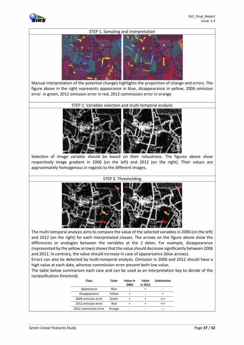
Green Linear Features Study Page 37 / 52
STEP 1. Sampling and interpretation
Manual interpretation of the potential changes highlights the proportion of change and errors. The figure above in the right represents appearance in blue, disappearance in yellow, 2006 omission error in green, 2012 omission error in red, 2012 commission error in orange
STEP 2. Variables selection and multi-temporal analysis
Selection of image variable should be based on their robustness. The figures above show respectively image gradient in 2006 (on the left) and 2012 (on the right). Their values are approximately homogenous in regards to the different images.
STEP 3. Thresholding
The multi-temporal analysis aims to compare the value of the selected variables in 2006 (on the left) and 2012 (on the right) for each interpretated classes. The arrows on the figure above show the differences or analogies between the variables at the 2 dates. For example, disappearance (represented by the yellow arrows) shows that the value should decrease significantly between 2006 and 2012. In contrary, the value should increase in case of appeareance (blue arrows). Errors can also be detected by multi-temporal analysis. Omission in 2006 and 2012 should have a high value at each date, whereas commission error present both low value. The table below summarizes each case and can be used as an interpretation key to decide of the reclassification threshold.
Class Color Value in 2006
Value in 2012
Subtraction
Appearance Blue - + -
Disappearance Yellow + - +
2009 omission error Green + + +++
2012 omission error Red + + +++
2012 commission error Orange - - ---

GLF_Final_Report Issue: 1.3
Green Linear Features Study Page 38 / 52
5. Conclusions & Recommendations
5.1. Evaluation if the developed methods can be applied for the EEA 39 area
The main challenges of the GLF layer production on the entire EEA 39 area lies in:
The production of a land cover data across a large territory (around 6,000,000 km²), which
means that processing chain should be designed to deal with large amount of data.
The respect of the homogeneity and consistency of the GLF layer across the overall area.
The application performed on the five study sites aims to ensure the reproducibility on the entire EEA
39 area. It showed that statistical results are globally homogenous across the different landscape and
data. However, look-and-feel analysis suggested that some areas are more complex to produce than
some others. For example, results of the Romanian site present more commission errors than the
others site. This illustrates the potential role of ancillary data such as the LPIS available on the overall
areas to limit heterogeneous results. Moreover, a classification strategy to reclassify local area
according their weakness should be complementary to the main classification methods.
The collection of training data is by far the most time consuming process because it currently involves
a relatively high degree of manual input. It also illustrates the need to foster consistent and
homogeneous interpretation rules to classify GLF across different landscapes. A mapping guide
organised according bio-geographical regions should be produced before the production work. This
approach also has to be completed by the collection of in situ ancillary data. The collection of training
data should be greatly facilitated when LPIS data will include the systematic collection of GLF as
discussed in Section 5.3.
Finally, it should be noted that the nomenclature proposed in section 3.4.2 would need to be further
simplified due to the limitation of the spatial and spectral resolution of the imagery used. An approach
based in the future, on SPOT-6&7 data or equivalent supplemented by Sentinel-2 should provide far
better results and should allow for a more complex nomenclature.
5.2. Estimations about the effort and cost for mapping the entire EEA 39 area
This section provides technical, methodological and management aspects defining the efforts and cost
for mapping the entire EEA 39 area. This evaluation is based on results obtained at the different
production step of this study. A summary of the findings are provided in Figure 19 below.

GLF_Final_Report Issue: 1.3
Green Linear Features Study Page 39 / 52
Figure 19. Summary of findings.
Technical aspects
Input Data Data is an essential aspect for the production a GLF layer. This study demonstrated that GLF can be
extracted from Spot-5 images (VHR2) based on an automated approach. However, the 2.5m spatial
resolution provided by the SPOT-5 sensor provide a slight blur and noise probably due to the
panchromatic supermode (which is a combination of two 5m resolution image). Some GLF can then be
extracted and analysed easily but some others cannot be delineated or characterized. This statement
is based both on visual and automated processing. This results in potential problems of quality, which
are independent from the methodological and technical aspects presented in section 5.2.1.2. A finer
resolution would then be recommended for future updates to provide more accurate results. VHR1
data such as Pleiades, Quickbird and WorldView can provide detailed information but SPOT-6&7
images are probably the best compromise for the mapping of the GLF.
Multitemporal information is really important to provide an accurate production of the GLF. The
monitoring of the GLF layer and change detection between 2006 and 2012 images demonstrated that
combination of image at 2 different dates can limit significantly the number of omission and
commission errors. Multi-temporal information is then recommended. VHR imagery could easily be
supplemented by Sentinel 2 data for future updates.
Ancillary data such as LPIS edges, OSM, HRL Forest Type were tested:
- LPIS edges used as a mask does not improve the extraction of GLF. Nevertheless, their use
should remain interesting as a support layer to perform massive sampling and validation.
- OSM can be used to classify automatically riparian elements. Nevertheless, this information
can be heterogeneous from a country to another and should be used jointly with other data
source.
- HRL Layer Forest Type can classify automatically numerous patches. It has been showed that
it is efficient for large patches. However even its MMU should be about 400m², it doesn’t
provide information for small patches.
Possible
• GLF binary mask
• GLF simplified nomenclature for tree features
• GLF update and enhancement
Difficult to achieve
• GLF detailed nomenclature including grassy features and tree alignement
Recommendations
• Multi-temporal dataset
• Finer spatial resolution (at least SPOT-6 data)
• Integration of ancillary data (HRL FTY for patches, OSM for riparian features, LPIS ).

GLF_Final_Report Issue: 1.3
Green Linear Features Study Page 40 / 52
A finer resolution (about 1.5 m), multi-temporal information and ancillary data availability constitute
undoubtedly the best conditions to extract the GLF.
Methodology Image variable computation and automatic classification can be time consuming. For example,
computation of GLCM needs an hour per image and the overall classification time is about 4 hours.
Application over the entire EEA 39 will then require dedicated hardware and source code optimization
based on High Performance Computing techniques.
To foster economies of scale and thus reduce production costs, the proposed methodology is based
on automated procedures. Results bring out that the extraction of undifferentiated GLF (GLF binary
mask) is achievable at the required level of accuracy (>85%). However their characterization is weaker
and cannot be acceptable without additional manual post-processing.
The definition of the detailed nomenclature constitutes the main criterion that defines the complexity
of the project. While the identification of GLF based on a limited number of classes is relatively
achievable (similar to that of the GLE layer for the Riparian Zones project) at the required level of
accuracy, a more detailed nomenclature will be more difficult to achieve without the help of additional
ancillary and/or visual interpretation. It was concluded that complex GLF such as grass filter bank,
stone walls and tree alignments cannot be extracted with the current imagery.
Moreover, discrimination between patch and linear features can be difficult without additional
specifications. This illustrates the issue of class definition and the difficulty to mix functional and
geometric properties of GLF. GLF can fit in several classes and classification is not obvious. The
nomenclature should require more detailed geometric specifications such as a width/length ratio.
Results provided by automatic processing were based on a semi-automated selection of training
samples. Experiments showed that results have a strong dependence to the quantity and quality of
samples. Even this step can be partially automated using HR Layer Forest Layer, a massive and accurate
characterization is important to produce a layer compliant with the GLF nomenclature. This task seems
to be achievable only by manual interpretation and brings out a potential time-consuming step in the
production chain. An alternative approach based on clustering methods and visual interpretation can
also be proposed. A clustering method classifying images without an a priori on expected class can be
applied on edges and classification will be done manually by selection of representative clusters. In
that way, sampling and classification are combined in a unique step. Further experiments should prove
if this approach can be used main processing chain or as a complementary method to reclassify specific
areas.
Monitoring and change detection methodologies are achievable even it showed that it is particularly
complex to extract changes. Changes are very few and a multi-temporal analysis includes omission and
commission errors as well as actual changes. An automatic procedure is proposed to extract changes
and characterize errors at both dates. Such an approach also contributes to the continuous
improvement of the GLF products.
Management aspects
Input Data The production of a GLF layer on the entire EEA 39 area implies the management of a huge amount of
image data. It means that the producer needs capacities to store and structure such data and define
an adapted processing chain.
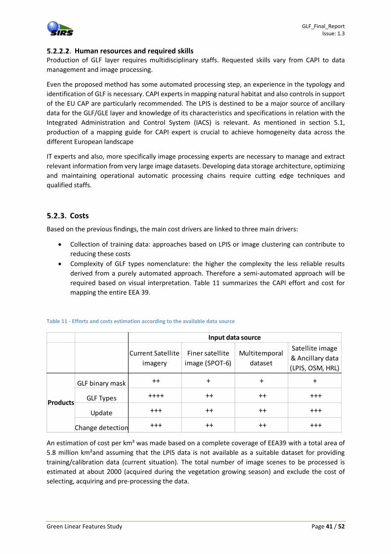
GLF_Final_Report Issue: 1.3
Green Linear Features Study Page 41 / 52
Human resources and required skills Production of GLF layer requires multidisciplinary staffs. Requested skills vary from CAPI to data
management and image processing.
Even the proposed method has some automated processing step, an experience in the typology and
identification of GLF is necessary. CAPI experts in mapping natural habitat and also controls in support
of the EU CAP are particularly recommended. The LPIS is destined to be a major source of ancillary
data for the GLF/GLE layer and knowledge of its characteristics and specifications in relation with the
Integrated Administration and Control System (IACS) is relevant. As mentioned in section 5.1,
production of a mapping guide for CAPI expert is crucial to achieve homogeneity data across the
different European landscape
IT experts and also, more specifically image processing experts are necessary to manage and extract
relevant information from very large image datasets. Developing data storage architecture, optimizing
and maintaining operational automatic processing chains require cutting edge techniques and
qualified staffs.
Costs
Based on the previous findings, the main cost drivers are linked to three main drivers:
Collection of training data: approaches based on LPIS or image clustering can contribute to
reducing these costs
Complexity of GLF types nomenclature: the higher the complexity the less reliable results
derived from a purely automated approach. Therefore a semi-automated approach will be
required based on visual interpretation. Table 11 summarizes the CAPI effort and cost for
mapping the entire EEA 39.
Table 11 - Efforts and costs estimation according to the available data source
An estimation of cost per km² was made based on a complete coverage of EEA39 with a total area of
5.8 million km²and assuming that the LPIS data is not available as a suitable dataset for providing
training/calibration data (current situation). The total number of image scenes to be processed is
estimated at about 2000 (acquired during the vegetation growing season) and exclude the cost of
selecting, acquiring and pre-processing the data.
Current Satellite
imagery
Finer satellite
image (SPOT-6)
Multitemporal
dataset
Satellite image
& Ancillary data
(LPIS, OSM, HRL)
GLF binary mask ++ + + +
GLF Types ++++ ++ ++ +++
Update +++ ++ ++ +++
Change detection +++ ++ ++ +++
Input data source
Products

GLF_Final_Report Issue: 1.3
Green Linear Features Study Page 42 / 52
The indicative cost estimates to produce each of the GLF binary and types layers assume that they are
produced together (some processing is combined) and would be as follows:
GLF Binary mask: 0.17€/km²
GLF Types layer: 0.18€/km²
The update and change detection indicative cost estimates also assume that these activities are
combined and are as follows:
GLF layer update: 0.09€/km²
Change detection: 0.08€/km²
This provides a combined cost of 0.52€/km² for the creation of the GLF layer and one update or
0.35€/km² for creation and 0.17€/km² for one update and change detection.
5.3. Proposal for the integration of LPIS data in the workflow
An assessment of the availability of LPIS data and its usefulness for the study was made for the 5 selected sites. LPIS data could be accessed for all but one test site (Sweden), but the data is only available from national web portals and downloading the data when available is only possible for limited areas not suitable for the purpose of this study. For France, it is possible to download LPIS data for the whole country, but only for agricultural parcels (not landscape features that include GLF). In any cases, landscape features are collected only when farmers are declaring them as part of their submission and the coverage is far from being complete. This is likely to change due to the CAP reform and several countries are now busy with updating their LPIS with the inclusion of landscape features (recent example of tenders from the Wallonia region in Belgium and for France). Even if this process is complete across the EU, this will only cover the EU territory partially (it is estimated that only 70-80% of the agricultural land use is covered by the LPIS. Therefore, a product covering the whole territory regardless of land use such as the GLF/GLE layer would still be needed. However, the exhaustive inclusion of GLF as part of the LPIS through the greening of the CAP could provide a very valuable source of training data. The LPIS could then be used to automatically select training data thus potentially reducing the cost of producing the GLF/GLE layer very significantly.
GLF_Final_Report Issue: 1.3
Green Linear Features Study Page 43 / 52
References
Aksoy, S., Akcay, H. G., & Wassenaar, T. (2010). Automatic Mapping of Linear Woody Vegetation Features in
Agricultural Landscapes Using Very High Resolution Imagery. IEEE Transactions on Geoscience and Remote
Sensing, 48(1), 511–522.
Baudry, J., Bunce, R. G. ., & Burel, F. (2000). Hedgerows: An international perspective on their origin, function
and management. Journal of Environmental Management, 60(1), 7–22.
Benediktsson, J., Swain, P. H., & Ersoy, O. K. (1990). Neural network approaches versus statistical methods in
classification of multisource remote sensing data. IEEE Transactions on Geoscience and Remote Sensing, 28(4),
540–552.
Bloch, I. (1996). Some aspects of Dempster-Shafer evidence theory for classification of multi-modality medical
images taking partial volume effect into account. Pattern Recognition Letters, 17(8), 905–919.
Coppin, P., Jonckheere, I., Nackaerts, K., Muy, B., & Lambin, E. F. (2004). Digital change detection methods in
ecosystem monitoring: a review. International Journal of Remote Sensing, 25, 1565–1596.
Duro, D. C., Franklin, S. E., & Dubé, M. G. (2012). A comparison of pixel-based and object-based image analysis
with selected machine learning algorithms for the classification of agricultural landscapes using SPOT-5 HRG
imagery. Remote Sensing of Environment, 118, 259–272.
Duda, R. O., Hart, P. E., & Stork, D. G. (2012). Pattern Classification (Vol. 2012, p. 680).
Fauvel, M., Arbelot, B., Benediktsson, J. A., Sheeren, D., & Chanussot, J. (2013). Detection of Hedges in a Rural
Landscape Using a Local Orientation Feature: From Linear Opening to Path Opening. IEEE Journal of Selected
Topics in Applied Earth Observations and Remote Sensing, 6(1), 15–26.
Fauvel, M., Chanussot, J., & Benediktsson, J. A. (2007). A Joint Spatial and Spectral SVMs Classification of
Panchromatic Images. In International Geoscience and Remote Sensing Symposium, IGARSS ’07 Conference,
2007 IEEE International, July 2007, Barcelona, Spain.
Forman, R. T. T., & Godron, M. (2008). Components Ecology Landscape Structural, 31(10), 733–740.
Haralick, R. M., Shanmugam, K., & Dinstein, I. (1973). Textural features for image classification. IEEE Transaction
on Systems, Man, and Cybernetics, 3, 610–621.
Jongman, R. (2004). Landscape linkages and biodiversity in European landscapes. In Springer (Ed.), The new
dimensions of the European landscape (pp. 179–189). Dordrecht.
Le Hegarat-Mascle, S., Bloch, I., & Vidal-Madjar, D. (1997). Application of Dempster-Shafer evidence theory to
unsupervised classification in multisource remote sensing. IEEE Transactions on Geoscience and Remote Sensing,
35(4), 1018–1031.
Lefebvre, A., Beaugendre, N., Pennec, A., Sannier, C., & Corpetti, T. (2013). Using data fusion to update built-up
areas of the 2012 European High-Resolution Layer Imperviousness. In 33rd EARSeL Symposium. Matera, Italy.
Lefebvre, A., Corpetti, T., & Hubert-Moy, L. (2011). Estimation of the orientation of textured patterns via wavelet
analysis. Pattern Recognition Letters, 32, 190–196.
Lennon, M., Mouchot, M. C., Mercier, G., & Hubert-Moy, L. (2000). Segmentation of hedges on CASI
hyperspectral images by data fusion from texture, spectral and shape analysis. In IGARSS 2000. IEEE 2000
International Geoscience and Remote Sensing Symposium. Taking the Pulse of the Planet: The Role of Remote
Sensing in Managing the Environment.
Li, C., Wang, J., Wang, L., Hu, L., & Gong, P. (2014). Comparison of Classification Algorithms and Training Sample
Sizes in Urban Land Classification with Landsat Thematic Mapper Imagery. Remote Sensing, 6(2), 964–983.

GLF_Final_Report Issue: 1.3
Green Linear Features Study Page 44 / 52
Lotfi, A., Javelle, A., Baudry, J., & Burel, F. (2010). Interdisciplinary Analysis of Hedgerow Network Landscapes’
Sustainability. Landscape Research, 35(4), 415–426.
Lu, Y. H., Trinder, J. C., & Kubik, K. (2006). Automatic Building Detection Using the Dempster-Shafer Algorithm.
Photogrammetric Engineering & Remote Sensing, 72(4), 395–403.
Ronfard, R. (1994). Region-based strategies for active contour models. International Journal of Computer Vision,
13(2), 229–251.
Serpico, S. B., & Bruzzone, L. (2001). A new search algorithm for feature selection in hyperspectral remote sensing
images. IEEE Transactions on Geoscience and Remote Sensing, 39(7), 1360–1367.
Van der Zanden, E. H., Verburg, P. H., & Mücher, C. A. (2013). Modelling the spatial distribution of linear
landscape elements in Europe. Ecological Indicators, 27, 125–136.
Vannier, C., & Hubert-Moy, L. (2008). Detection of Wooded Hedgerows in High Resolution Satellite Images using
an Object-Oriented Method. In IGARSS 2008 - 2008 IEEE International Geoscience and Remote Sensing
Symposium (Vol. 4, pp. IV – 731–IV – 734).

GLF_Final_Report Issue: 1.3
Green Linear Features Study Page 45 / 52
6. ANNEX 1: Comparison between GLF layer and HRL Tree Cover
Density layer

GLF_Final_Report Issue: 1.3
Green Linear Features Study Page 46 / 52

GLF_Final_Report Issue: 1.3
Green Linear Features Study Page 47 / 52

GLF_Final_Report Issue: 1.3
Green Linear Features Study Page 48 / 52

GLF_Final_Report Issue: 1.3
Green Linear Features Study Page 49 / 52

GLF_Final_Report Issue: 1.3
Green Linear Features Study Page 50 / 52
7. ANNEX 2: contribution of national LPIS web services

GLF_Final_Report Issue: 1.3
Green Linear Features Study Page 51 / 52
Screenshot of the Romanian LPIS web service composed of a viewer and a set of limited data. Data
download is not available
Screenshot of the Czech LPIS web service composed of a viewer and a set of limited data. Download
is available but limited by the viewer extent

GLF_Final_Report Issue: 1.3
Green Linear Features Study Page 52 / 52
Example of GLF not included in the Czech LPIS: Tree along roads, ditches and inside parks are not
delineated
Example of GLF include in the Romanian LPIS but not delineated. GLF are part of agricultural parcels,
not individual objects.