feature-based robust techniques for speech recognition · feature-based robust techniques for...
TRANSCRIPT
Nanyang Technological University
Feature-based Robust TechniquesFor Speech Recognition
A thesis submitted to the School of Computer Science and Engineeringof the Nanyang Technological University
by
Nguyen Duc Hoang Ha
in partial fulfilment of the requirementsto the Degree of Doctor of Philosophy
2016
Abstract
Automatic speech recognition (ASR) decodes speech signals into text. While ASR can
produce accurate word recognition in clean environment, its accuracy degrades consider-
ably under noisy conditions. I.e., robustness of ASR systems for real-world applications
remains a challenge. In this thesis, speech feature enhancement and model adaptation for
robust speech recognition is studied, and three novel methods to improve performance
are introduced.
The first work proposes a modification of the spectral subtraction method to reduce
the non-stationary characteristics of additive noise in the speech. The main idea is to first
normalise the noise’s characteristics towards a Gaussian noise model, and then tackle the
remaining noise by a model compensation method. The strategy is to reduce the noise
handling problem to the back-end process. In this work, the back-end compensation
process is applied using the vector Taylor series (VTS) model compensation approach,
and we call this method the noise normalization VTS (NN-VTS).
The second work proposes an extension of particle filter compensation (PFC) for the
large vocabulary continuous speech recognition (LVCSR) task. PFC is a clean speech
features tracking method using side information from hidden Markov models (HMM)
for the particle filter framework. However, under noisy conditions for sub-word based
LVCSR, the task to obtain an accurately aligned state sequence of HMM that describe
the underlying clean speech features is challenging. This is because the total number
of triphone models involved can be very large. To improve the identification of correct
phone sequence, this work proposes to use a noisy model HMM trained from noisy data
to estimate the state sequence and a parallel clean model HMM trained from clean data
to generate the clean speech features. These two HMMs are trained jointly, and the
alignment of states between the clean and noisy models HMM is obtained by single pass
i
retraining (SPR) technique. With this approach, the accuracy of state sequence estimate
is improved by the noisy model HMM, and the accurately aligned state is obtained by
SPR technique. When the missing side information for PFC is available, a word error
reduction of 28.46% from multi-condition training is observed for the Aurora-4 task.
The third work proposes a novel spectro-temporal transform framework to improve
word error rate for the noisy and reverberant environments. Motivated by the findings
that human speech comprehension relies on both the spectral content and temporal
envelope of speech signal, a spectro-temporal (ST) transform framework is proposed.
This framework adapts the features to minimize the mismatch between the input features
and training data using the Kullback Leibler divergence based cost function. In our work,
we examined two implementations to overcome the limited adaptation data issue. The
first implementation is a cross transform which is a sparse spectro-temporal transforms.
The second implementation is a cascaded transform of temporal transform and spectral
transform. Experiments are conducted on the REVERB Challenge 2014 task, where
clean and multi-condition trained acoustic models are tested with real reverberant and
noisy speech. Experimental results confirmed that temporal information is important
for reverberant speech recognition and the simultaneous use of spectral and temporal
information for feature adaptation is effective.
ii
Acknowledgments
I would like to express my sincere thanks and appreciation to my supervisor, Dr. Eng
Siong Chng (Nanyang Technological University, NTU), and co-supervisor, Dr. Haizhou
Li (Institute for Infocomm Research, I2R) for their invaluable guidance, patience, moti-
vation, and immense knowledge. Besides my supervisors, my sincere thanks also go to
Dr. Xiong Xiao (NTU) for his help and discussion during my PhD study time. Their
guidance helped me in all the time of research and writing of this thesis.
My sincere thanks also go to Prof. Chin-Hui Lee and Dr. Aleem Mushtaq for their
help, discussions, and guidance on the study of particle filter compensation (PFC) during
my internship in Georgia Institute of Technology. Without their help, my work on PFC
will be much more difficult to accomplish.
I also want to thank all my colleagues in the speech group in NTU for their help and
support in a variety of ways. My life is much more colourful and comfortable with their
friendship.
Last but not least, I would like to thank my family in Vietnam, for their constant
love and encouragement.
iii
Contents
Abstract . . . . . . . . . . . . . . . . . . . . . . . . . . . . . . . . . . . . . . i
Acknowledgments . . . . . . . . . . . . . . . . . . . . . . . . . . . . . . . . iii
List of Figures . . . . . . . . . . . . . . . . . . . . . . . . . . . . . . . . . . viii
List of Tables . . . . . . . . . . . . . . . . . . . . . . . . . . . . . . . . . . . x
List of Abbreviations . . . . . . . . . . . . . . . . . . . . . . . . . . . . . . xii
List of Notations . . . . . . . . . . . . . . . . . . . . . . . . . . . . . . . . . xiii
1 Introduction 1
2 Robust Techniques in Automatic Speech Recognition 5
2.1 Automatic Speech Recognition . . . . . . . . . . . . . . . . . . . . . . . . 5
2.2 Robust Speech Recognition . . . . . . . . . . . . . . . . . . . . . . . . . 11
2.2.1 Feature-based Robust Techniques . . . . . . . . . . . . . . . . . . 12
2.2.2 Model-based Robust Techniques . . . . . . . . . . . . . . . . . . . 21
2.3 Chapter Summary . . . . . . . . . . . . . . . . . . . . . . . . . . . . . . 33
3 Combination of Feature Enhancement and VTS Model Compensation
for Non-stationary Noisy Environments 34
3.1 Overview of the Proposed Framework . . . . . . . . . . . . . . . . . . . . 36
3.2 Feature Enhancement . . . . . . . . . . . . . . . . . . . . . . . . . . . . . 37
3.3 Relationship Between Clean and Enhanced Features . . . . . . . . . . . . 38
3.4 Approximations of Noisy Acoustic Models . . . . . . . . . . . . . . . . . 39
3.5 Discussions on Back-end Model Compensation . . . . . . . . . . . . . . . 41
3.6 Experiments . . . . . . . . . . . . . . . . . . . . . . . . . . . . . . . . . . 44
3.6.1 Database . . . . . . . . . . . . . . . . . . . . . . . . . . . . . . . 44
iv
3.6.2 System Configurations . . . . . . . . . . . . . . . . . . . . . . . . 45
3.7 Summary . . . . . . . . . . . . . . . . . . . . . . . . . . . . . . . . . . . 47
4 A Particle Filter Compensation Approach to Robust LVCSR 49
4.1 Introduction . . . . . . . . . . . . . . . . . . . . . . . . . . . . . . . . . . 49
4.2 Tracking Sequence of Clean Speech Features using PFC . . . . . . . . . . 51
4.2.1 Using HMM States to Generate Samples . . . . . . . . . . . . . . 51
4.2.2 Distortion Model . . . . . . . . . . . . . . . . . . . . . . . . . . . 52
4.2.3 A Brief Discussion of using PFC . . . . . . . . . . . . . . . . . . . 53
4.3 PFC for LVCSR . . . . . . . . . . . . . . . . . . . . . . . . . . . . . . . . 54
4.4 Aurora-4 Experiments . . . . . . . . . . . . . . . . . . . . . . . . . . . . 57
4.4.1 General Configurations . . . . . . . . . . . . . . . . . . . . . . . . 57
4.4.2 Experiments with Oracle Cluster ID . . . . . . . . . . . . . . . . 57
4.4.3 Experiments with Estimated Cluster ID . . . . . . . . . . . . . . 59
4.5 Summary and Future Work . . . . . . . . . . . . . . . . . . . . . . . . . 61
5 Feature Adaptation Using Spectro-Temporal Information 62
5.1 Introduction . . . . . . . . . . . . . . . . . . . . . . . . . . . . . . . . . . 63
5.2 Generalized Linear Transform for Feature Adaptation . . . . . . . . . . . 66
5.3 Review of Maximum Likelihood Based Feature Adaptation . . . . . . . . 68
5.4 Minimum Kullback-Leibler (KL) Divergence Criterion . . . . . . . . . . . 69
5.4.1 Objective function . . . . . . . . . . . . . . . . . . . . . . . . . . 69
5.4.2 EM Algorithm for Parameter Estimation . . . . . . . . . . . . . . 72
5.5 A Unified Perspective on Feature Processing . . . . . . . . . . . . . . . . 74
5.6 Implementation Issues . . . . . . . . . . . . . . . . . . . . . . . . . . . . 75
5.6.1 Sparse Generalized Linear Transform . . . . . . . . . . . . . . . . 75
5.6.2 Cascaded Transform . . . . . . . . . . . . . . . . . . . . . . . . . 77
5.6.3 Interpolation of Statistics . . . . . . . . . . . . . . . . . . . . . . 78
5.7 Experimental Study on Spectro-Temporal Transform . . . . . . . . . . . 79
5.7.1 Experimental Settings . . . . . . . . . . . . . . . . . . . . . . . . 79
5.7.2 Effect of Window Length L . . . . . . . . . . . . . . . . . . . . . 82
5.7.3 Spectral, Temporal, and Spectro-Temporal Transforms . . . . . . 84
v
5.7.4 Experiments for Cascaded Transforms . . . . . . . . . . . . . . . 85
5.7.5 Hybrid Adaptation and Statistics Smoothing . . . . . . . . . . . . 86
5.7.6 Combination of Feature Adaptation and Model Adaptation . . . . 89
5.8 Chapter Summary . . . . . . . . . . . . . . . . . . . . . . . . . . . . . . 89
6 Conclusions 91
6.1 Contributions and Discussions . . . . . . . . . . . . . . . . . . . . . . . . 91
6.1.1 Noise Conditioning/Normalization Vector Taylor Series Method . 91
6.1.2 PFC framework for LVCSR . . . . . . . . . . . . . . . . . . . . . 92
6.1.3 Spectro-Temporal Transform . . . . . . . . . . . . . . . . . . . . . 93
6.2 Future Directions . . . . . . . . . . . . . . . . . . . . . . . . . . . . . . . 94
vi
List of Publications
[1] Duc Hoang Ha Nguyen, Xiong Xiao, Eng Siong Chng, and Haizhou Li.An analysis of vector taylor series model compensation for non-stationarynoise in speech recognition. In ISCSLP, Hong Kong, 2012.
[2] Duc Hoang Ha Nguyen, Aleem Mushtaq, Xiong Xiao, Eng SiongChng, Haizhou Li, and Chin-Hui Lee. A particle filter compensationapproach to robust lvcsr. In APSIPA ASC, Taiwan, 2013.
[3] Duc Hoang Ha Nguyen, Xiong Xiao, Eng Siong Chng, and HaizhouLi. Generalization of temporal filter and linear transformation for robustspeech recognition. In ICASSP, Italy, 2014.
[4] Duc Hoang Ha Nguyen, Xiong Xiao, Eng Siong Chng, and HaizhouLi. Feature adaptation using linear spectro-temporal transform for ro-bust speech recognition. IEEE/ACM Transactions on Audio, Speech,and Language Processing, PP(99):1–1, 2016.
vii
List of Figures
2.1 The architecture of a statistical ASR system. . . . . . . . . . . . . . . . . 7
2.2 The left-to-right HMM with three emitting hidden states . . . . . . . . . 9
2.3 The left-to-right HMM represented as a DBN . . . . . . . . . . . . . . . 10
2.4 An illustration of mismatch between trained acoustic model and test features 12
2.5 Feature-based noise robust speech recognition system . . . . . . . . . . . 13
2.6 Model-based noise robust speech recognition system . . . . . . . . . . . . 13
2.7 An illustration of effects of mean and variance normalization on speech
features. . . . . . . . . . . . . . . . . . . . . . . . . . . . . . . . . . . . . 15
3.1 The proposed framework of combination of feature enhancement and the
VTS model compensation. . . . . . . . . . . . . . . . . . . . . . . . . . . 35
3.2 An illustration of residual noise. . . . . . . . . . . . . . . . . . . . . . . . 39
3.3 An illustration of the scale function (1− α)2 + α2 in range [0, 1] . . . . . 42
3.4 An example of the noise model GMM with 2 mixtures . . . . . . . . . . . 42
3.5 An illustration of the key idea of the proposed noise normalization method. 43
3.6 An example of the smoothed version of the ideal noise in log-Mel domain. 45
3.7 Effects of the proposed noise normalization method . . . . . . . . . . . . 47
4.1 HMM for sample generation . . . . . . . . . . . . . . . . . . . . . . . . . 52
4.2 A block diagram illustrates training process using the single-pass retraining
(SPR). . . . . . . . . . . . . . . . . . . . . . . . . . . . . . . . . . . . . . 55
4.3 A block diagram illustrates oracle experiment vs. actual experiment. . . . 58
4.4 Performance of PFC with different numbers of clusters . . . . . . . . . . 60
5.1 An illustration of a feature adaptation system . . . . . . . . . . . . . . . 63
viii
5.2 Illustrations of 5 types of linear transform-based feature adaptation . . . 64
5.3 An illustration of the Spectro-Temporal feature transform, or ST trans-
form, in Eq 5.1. . . . . . . . . . . . . . . . . . . . . . . . . . . . . . . . . 66
5.4 Illustrations of 5 special cases of ST transform W . . . . . . . . . . . . . 67
5.5 Combinations of fMLLR and temporal filter in tandem. . . . . . . . . . 77
5.6 Effects of the input window length of the ST transforms on WER on dev
set of REVERB Challenge 2014 . . . . . . . . . . . . . . . . . . . . . . . 83
5.7 Log likelihood per frame averaged over the eval set . . . . . . . . . . . . 88
ix
List of Tables
3.1 The settings for baseline system . . . . . . . . . . . . . . . . . . . . . . . 46
4.1 Word accuracy (%) obtained by PFC using oracle cluster ID information 59
4.2 Word accuracy (%) obtained by PFC using estimated cluster IDs and
WITH re-computed the dynamic features. . . . . . . . . . . . . . . . . . 60
4.3 Word accuracy (%) obtained by PFC using estimated cluster IDs and
WITHOUT re-computing the dynamic features. . . . . . . . . . . . . . . 61
5.1 Estimation of W to minimize the cost function in (5.11) . . . . . . . . . 72
5.2 Eight special cases of the ST transform in (5.1) and the minimum KL
divergence objective function in (5.11) . . . . . . . . . . . . . . . . . . . 74
5.3 Performance of feature adaptation in WER (%) for the eval set of RE-
VERB Challenge 2014 . . . . . . . . . . . . . . . . . . . . . . . . . . . . 84
5.4 Performance of cascaded transforms in WER (%) for the eval set . . . . . 85
5.5 WER (%) of hybrib mode adaptation with statistics smoothing on the eval
set . . . . . . . . . . . . . . . . . . . . . . . . . . . . . . . . . . . . . . . 87
5.6 WER (%) on the eval set by combining the best ST transform and a
256-class CMLLR model adaptation. . . . . . . . . . . . . . . . . . . . . 89
x

xi
List of Abbreviations
AM Acoustic ModelARMA Autoregressive Moving AverageASR Automatic Speech RecognitionCAT Cluster Adaptive TrainingCMLLR Constrained MLLRCMN Cepstral Mean NormalizationCSR Continuous Speech RecognitionCVN Cepstral Variance NormalizationDBN Dynamic Bayes NetworkDCT Discrete Cosine TransformEM Expectation MaximizationGMM Gaussian Mixture ModelHEQ Histogram EqualizationHLDA Heteroscedastic Linear Discriminant AnalysisHMM Hidden Markov ModelIDCT Inverse Discrete Cosine TransformJSTN Joint Spectral and Temporal NormalizationLM Language ModelLVCSR Large Vocabulary Continuous Speech RecognitionMAP Maximum A PosterioriMFCC Mel-Frequency Cepstral CoefficientML Maximum LikelihoodMLLR Maximum Likelihood Linear RegressionMMSE Minimum Mean Square ErrorPCA Principal Component AnalysisPFC Particle Filter CompensationPLP Perceptual Linear PredictivePMC Parallel Model CombinationRASTA Relative SpectraSNR Signal to Noise RatioSS Spectral SubtractionST-Transform Spectro-Temporal TransformTSN Temporal Structure NormalizationVTS Vector Taylor Series
xii
List of Notations
mathematical operations
E [f(x)] the expected value of function f(x) where x is a random variablef(x) ? g(x) Convolution of f(x) with g(x)∂f(x)/∂x partial derivative of f with respect to xf(x)|a = f(a) the value of function f where x = a∂f(x)∂x|a the value of function ∂f
∂xwhere x = a
fA ◦ fB the cascaded transform of fA and fB transforms
vectors and matricesRd d-dimensional Euclidean spacex,x normal-face is used for scalar and bold-face for column vectorA bold-face capital letter is used for matrixA−1 the inverse of matrix AxT transpose of vector x‖x‖ Euclidean norm of vector x
probability, distributions
P (·) probabilityp(·) probability densityPr{·} the probability of a condition being metp(x|θ) the conditional probability density of x given θ
xiii
Chapter 1
Introduction
Automatic speech recognition (ASR) decodes speech signals into text [1]. The perfor-
mance of ASR systems has improved greatly in recent years due to more training data,
increased computational power, and deep learning algorithm for acoustic modelling [2].
While ASR is expected to produce accurate word recognition in clean environment, its
accuracy degrades considerably in noisy and reverberant acoustic environments. Ro-
bustness of ASR systems in adverse environments for real-world applications remains a
challenge. In this thesis, speech feature enhancement and model adaptation in robust
speech recognition is investigated and three novel techniques are proposed to improve
word error rate of speech recognition system in noisy and reverberant environments.
Research in robust speech recognition has a rich history and many techniques have
been proposed in the last three decades. They can be broadly categorized into two
major approaches: model-based and feature-based approaches. Model-based techniques
aim to update the acoustic model to better represent speech features under new test
conditions. Examples include maximum a-posteriori (MAP) adaptation [3], maximum
likelihood linear regression (MLLR) [4, 5] and their variants [6–9], and vector Taylor se-
ries (VTS) based adaptation [10–12]. Feature-based techniques, on the other hand, aim
to bring speech signals/features closer to the ones used during training. Examples in-
clude: speech enhancement methods such as spectral subtraction [13], Wiener filter [14],
minimum mean square error (MMSE) short time spectral amplitude estimator [15, 16];
dereverberation [17–22]; feature compensation methods such as SPLICE [23]; feature
normalization methods such as cepstral mean normalization (CMN) [24], mean and vari-
ance normalization (MVN) [25], histogram equalization (HEQ) [26]; temporal filters such
1
Chapter 1. Introduction
as Relative spectral processing (RASTA) [27, 28]; and linear feature transform such as
feature-space MLLR (fMLLR) [4, 29]. For a comprehensive review of the existing tech-
niques, readers are referred to [30–32].
Feature and model-based approaches have their own advantages and limitations. Gen-
erally speaking, feature-based approach may be less powerful than model based approach
as it does not have access to the acoustic model. However, feature-based approach is more
computationally efficient than model-based approach, and is easier to integrate it into
ASR systems as it does not require modifications to the decoder.
In this thesis, three novel feature and model based techniques are proposed to improve
word error rate of speech recognition system in mismatch conditions. The general research
challenge is how to train acoustic model on one domain and test on other domain. The
three proposed techniques are extensions, combinations and improvements of existing
techniques, which are detailed in the following text.
Noise Normalization - VTS (NN-VTS) [33] Chapter 3 discusses this work. The
aim of the first work attempts to reduce the non-stationary characteristics of the
additive noise in the speech. The motivation is to utilize the feature-based approach
to facilitate the back-end compensation. Particularly, in the front-end, a modifica-
tion of spectral subtraction method [13] is proposed to first normalise noise charac-
teristics towards a Gaussian noise model, and then, in the back-end, vector Taylor
series (VTS) model compensation [11] is applied to compensate for the residual
noise. With the proposed noise normalization process, the back-end compensation
does not need to be updated or have increased in complexity when noise changes.
This method is called noise normalization VTS (NN-VTS) and experimental study
on the Aurora-2 task shows that significant performance improvement is possible
over conventional VTS model compensation.
Particle Filter Compensation (PFC) for LVCSR system [34] Chapter 4 discusses
the second work in which a particle filter compensation (PFC) method [35] is ex-
tended to estimate clean speech features for the large vocabulary continuous speech
recognition (LVCSR) task. PFC utilizes side information from hidden Markov mod-
els (HMM) for the particle filter framework to track the clean speech features. The
2
Chapter 1. Introduction
side information from HMM here is the aligned state sequence of HMM that de-
scribe the underlying clean speech features. However under noisy conditions for
sub-word based LVCSR, the task to obtain accurate side information is challenging
as a large number of triphone models are involved in LVCSR system. To improve
the identification of correct state sequence, a noisy model HMM trained from noisy
data is used to estimate the state sequence and a parallel clean model HMM trained
from clean data is used to generate the clean speech samples. These two HMMs
are trained jointly using single pass retraining (SPR) technique to obtain the align-
ment of states between the clean and noisy models HMMs. With this approach,
the accuracy of state sequence is improved by the noisy acoustic model and the
accurately aligned states are obtained by the SPR technique. Experimental study
is conducted on the Aurora-4 task and the results show a word error reduction of
28.46% from multi-condition training when the missing side information for PFC
is available.
Spectro-Temporal (ST) transform [36,37] The third work discussed in Chapter 5
proposes a novel linear feature transformation to compensate for background noise
and reverberation. Motivated by the findings that both the spectral content and
temporal envelope of speech signal affect human speech comprehension, a spectro-
temporal (ST) transform framework is proposed. The ST transform modifies the
input features to minimize its mismatch to the training data using the Kullback
Leibler divergence cost function. To cope with the limited adaptation data issue,
two implementations of the ST transform are examined. The first implementa-
tion is a sparse ST transform where estimated parameters are manually selected
to utilize most of the temporal and spectral information for the speech feature
processing. This transform uses data covering a cross in the speech features, and
thus we call it the cross transform. The second implementation decomposes the
ST transform into temporal filter and spectral transform. In other words, the new
ST transform is a combination of temporal filter and spectral transform in tandem.
Experiments are conducted on the REVERB Challenge 2014 task, and the acoustic
model is trained on clean speech data, and tested with real reverberant and noisy
3
Chapter 1. Introduction
speech. Both implementations of ST transform were showed to be effective and ex-
perimental results suggest that temporal information is important for reverberant
speech recognition, and the simultaneous use of spectral and temporal information
for feature adaptation is complementary.
This thesis is structured as follows. Chapter 2 will review further in details robust
speech recognition. Chapter 3, 4 and 5 will present the first work (noise normalization
VTS), the second work (extension of PFC) and the third work (ST transform), respec-
tively. Chapter 6 will conclude the contributions in this thesis and discuss some future
extension works.
4
Chapter 2
Robust Techniques in AutomaticSpeech Recognition
In this chapter, a review of noise robust speech recognition techniques is presented. As
statistical hidden Markov model (HMM)-based speech recognition system is used as a
baseline ASR framework, a brief description of the HMM-based ASR system is first
provided. A detailed review of ASR techniques can be found in [1]. Secondly, robust
techniques are presented to cope with distortions of speech signal under noisy conditions.
Generally speaking, noise robust techniques can be grouped into two classes, i.e. the
feature space techniques that process speech features to reduce noise effects, and the
model space techniques that modify the acoustic model to fit the noisy features. As
three proposed works in this thesis are feature-based techniques, this class of techniques
are emphasized, and to be complete, model-based techniques are also briefly reviewed.
2.1 Automatic Speech Recognition
The objective of automatic speech recognition (ASR) is to correctly convert a speech
signal to the sequence of words conveyed by the signal. As the speech signal itself is not
a good representation for ASR, it is usually converted into a sequence of feature vectors,
X = {x1,x2, · · · ,xT}, where xt is a feature vector extracted at time t. This process
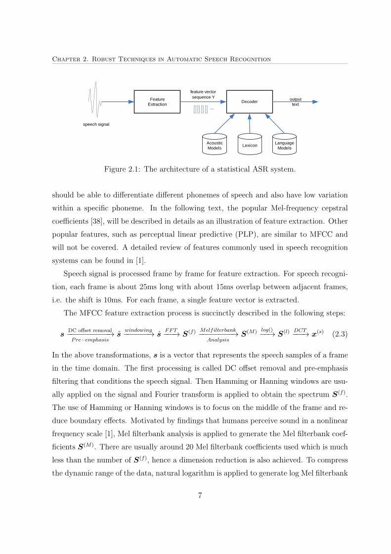
is called feature extraction as shown in Fig. 2.1. The feature vector sequence is then
processed by a decoder for recognition. The recognition problem is typically formulated
5
Chapter 2. Robust Techniques in Automatic Speech Recognition
as follows
w = arg maxw
P (w|X) (2.1)
where w = {w1, w2, · · · , wL} represents a word sequence, P (w|X) is the posterior prob-
ability of w given X, and w is the most likely word sequence.
Rather than modelling the posterior P (w|X) directly, Bayes’ rule is commonly used
to transform the original problem in (2.1) into an equivalent problem as follows [1]
w = arg maxw
P (X|w)P (w)
P (X)
= arg maxw
P (X|w)P (w) (2.2)
where P (X|w) represents the probability of the feature vector sequence X generated by
the word sequence w and P (X|w) is commonly known as the acoustic likelihood score.
The prior P (w) is the probability of the word sequence w and is called the language
model score. In practice, the evaluation of P (X|w) is by an acoustic model, e.g. Gaus-
sian mixture model hidden Markov model (GMM-HMM), and P (w) is by a language
model (LM), e.g. n-gram model [1]. The acoustic model captures the conditional distri-
bution of the feature vectors given a speech class, such as phoneme, while the language
model captures the joint probability of a sequence of words. Another model, called pro-
nunciation model (PM), also commonly known as lexicon, is used to link the acoustic
model and language model. The pronunciation model is usually in the form of a pronun-
ciation dictionary, which defines a phoneme sequence for each word in the vocabulary of
the system. The AM, LM, and PM are all used by the decoder to build a search space
that represents all possible word/phoneme sequences allowed in the ASR system. The
decoder then find the most likely word sequences in the search space.
In the following sections, two ASR modules that are relevant to the topic of this thesis
will be described in more details, i.e. the feature extraction and the acoustic model.
Feature Extraction
The feature extraction process aims to transform the speech signal to a compact form
of speech features that contains discriminative information. Suitable features for ASR
6
Chapter 2. Robust Techniques in Automatic Speech Recognition
speech signal
FeatureExtraction
Decoder
feature vectorsequence Y output
text...
Acoustic Models
Lexicon LanguageModels
Figure 2.1: The architecture of a statistical ASR system.
should be able to differentiate different phonemes of speech and also have low variation
within a specific phoneme. In the following text, the popular Mel-frequency cepstral
coefficients [38], will be described in details as an illustration of feature extraction. Other
popular features, such as perceptual linear predictive (PLP), are similar to MFCC and
will not be covered. A detailed review of features commonly used in speech recognition
systems can be found in [1].
Speech signal is processed frame by frame for feature extraction. For speech recogni-
tion, each frame is about 25ms long with about 15ms overlap between adjacent frames,
i.e. the shift is 10ms. For each frame, a single feature vector is extracted.
The MFCC feature extraction process is succinctly described in the following steps:
sDC offset removal−−−−−−−−−−→Pre−emphasis
swindowing−−−−−−→ s
FFT−−−→ S(f) Melfilterbank−−−−−−−−→Analysis
S(M) log()−−→ S(l) DCT−−−→ x(s) (2.3)
In the above transformations, s is a vector that represents the speech samples of a frame
in the time domain. The first processing is called DC offset removal and pre-emphasis
filtering that conditions the speech signal. Then Hamming or Hanning windows are usu-
ally applied on the signal and Fourier transform is applied to obtain the spectrum S(f).
The use of Hamming or Hanning windows is to focus on the middle of the frame and re-
duce boundary effects. Motivated by findings that humans perceive sound in a nonlinear
frequency scale [1], Mel filterbank analysis is applied to generate the Mel filterbank coef-
ficients S(M). There are usually around 20 Mel filterbank coefficients used which is much
less than the number of S(f), hence a dimension reduction is also achieved. To compress
the dynamic range of the data, natural logarithm is applied to generate log Mel filterbank
7
Chapter 2. Robust Techniques in Automatic Speech Recognition
coefficients S(l). The use of logarithm is also motivated by psychoacoustic findings that
humans perceive loudness roughly in proportion to the logarithm of energy [39], though
measured loudness scales more precise than the logarithm exist [40]. Finally, discrete
cosine transform (DCT) is applied on S(l) and the first half of the DCT coefficients x(s)
that contain discriminative information are used for speech recognition. Another advan-
tage of using DCT is that it significantly decorrelates S(l) such that diagonal instead of
full covariance matrix could be used in the acoustic model which significantly reduces
the number of parameters in the model.
The obtained features x(s) is usually called static features as they only contain the
spectral information of speech signal within a frame and do not contain temporal in-
formation across frames. As speech signals are slowly varying, there is high correlation
between neighboring frames that could be exploited for speech recognition. To capture
the temporal information across frames, dynamic features [41] are extracted and concate-
nated with the static features to improve the discriminative capability and robustness of
the features. Usually, the first-order (delta) and the second-order (delta-delta) dynamic
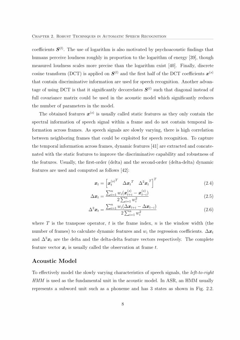
features are used and computed as follows [42]:
xt =[x
(s)t
T∆xt
T ∆2xtT]T
(2.4)
∆xt =
∑ni=1wi(x
(s)t+i − x
(s)t−i)
2∑n
i=1w2i
(2.5)
∆2xt =
∑ni=1wi(∆xt+i −∆xt−i)
2∑n
i=1w2i
(2.6)
where T is the transpose operator, t is the frame index, n is the window width (the
number of frames) to calculate dynamic features and wi the regression coefficients. ∆xt
and ∆2xt are the delta and the delta-delta feature vectors respectively. The complete
feature vector xt is usually called the observation at frame t.
Acoustic Model
To effectively model the slowly varying characteristics of speech signals, the left-to-right
HMM is used as the fundamental unit in the acoustic model. In ASR, an HMM usually
represents a subword unit such as a phoneme and has 3 states as shown in Fig. 2.2.
8
Chapter 2. Robust Techniques in Automatic Speech Recognition
s2 s3 s4
State 1 2 3 4 5
Non emitting state
Emitting state
Allowed transition
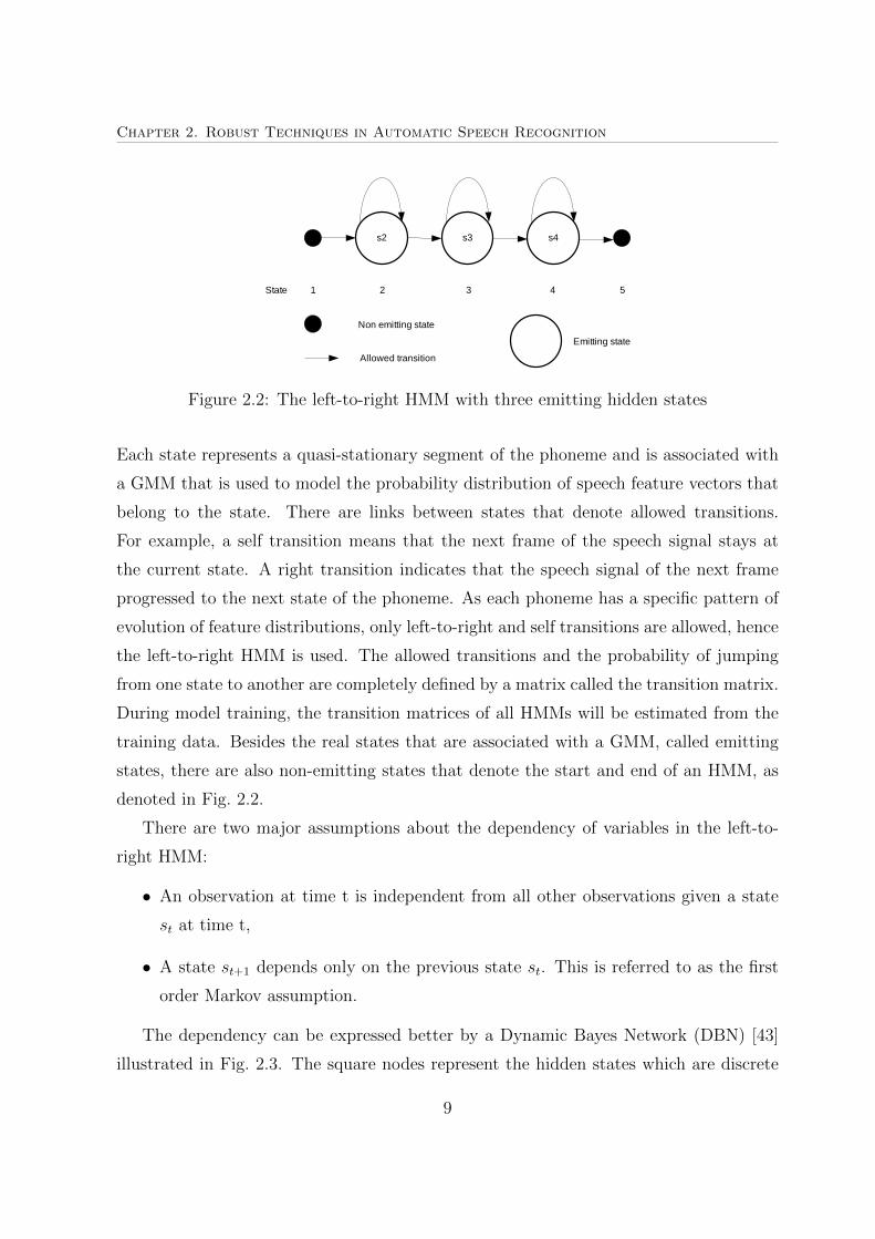
Figure 2.2: The left-to-right HMM with three emitting hidden states
Each state represents a quasi-stationary segment of the phoneme and is associated with
a GMM that is used to model the probability distribution of speech feature vectors that
belong to the state. There are links between states that denote allowed transitions.
For example, a self transition means that the next frame of the speech signal stays at
the current state. A right transition indicates that the speech signal of the next frame
progressed to the next state of the phoneme. As each phoneme has a specific pattern of
evolution of feature distributions, only left-to-right and self transitions are allowed, hence
the left-to-right HMM is used. The allowed transitions and the probability of jumping
from one state to another are completely defined by a matrix called the transition matrix.
During model training, the transition matrices of all HMMs will be estimated from the
training data. Besides the real states that are associated with a GMM, called emitting
states, there are also non-emitting states that denote the start and end of an HMM, as
denoted in Fig. 2.2.
There are two major assumptions about the dependency of variables in the left-to-
right HMM:
• An observation at time t is independent from all other observations given a state
st at time t,
• A state st+1 depends only on the previous state st. This is referred to as the first
order Markov assumption.
The dependency can be expressed better by a Dynamic Bayes Network (DBN) [43]
illustrated in Fig. 2.3. The square nodes represent the hidden states which are discrete
9
Chapter 2. Robust Techniques in Automatic Speech Recognition
st=i st+1= j
ot=x t ot+1=x t+1
aij
bi(x t) b j(x t+1)
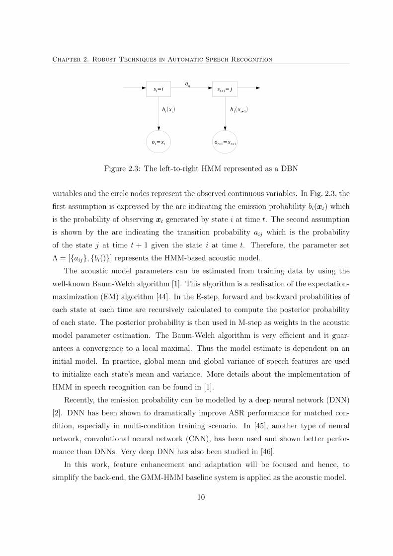
Figure 2.3: The left-to-right HMM represented as a DBN
variables and the circle nodes represent the observed continuous variables. In Fig. 2.3, the
first assumption is expressed by the arc indicating the emission probability bi(xt) which
is the probability of observing xt generated by state i at time t. The second assumption
is shown by the arc indicating the transition probability aij which is the probability
of the state j at time t + 1 given the state i at time t. Therefore, the parameter set
Λ = [{aij}, {bi()}] represents the HMM-based acoustic model.
The acoustic model parameters can be estimated from training data by using the
well-known Baum-Welch algorithm [1]. This algorithm is a realisation of the expectation-
maximization (EM) algorithm [44]. In the E-step, forward and backward probabilities of
each state at each time are recursively calculated to compute the posterior probability
of each state. The posterior probability is then used in M-step as weights in the acoustic
model parameter estimation. The Baum-Welch algorithm is very efficient and it guar-
antees a convergence to a local maximal. Thus the model estimate is dependent on an
initial model. In practice, global mean and global variance of speech features are used
to initialize each state’s mean and variance. More details about the implementation of
HMM in speech recognition can be found in [1].
Recently, the emission probability can be modelled by a deep neural network (DNN)
[2]. DNN has been shown to dramatically improve ASR performance for matched con-
dition, especially in multi-condition training scenario. In [45], another type of neural
network, convolutional neural network (CNN), has been used and shown better perfor-
mance than DNNs. Very deep DNN has also been studied in [46].
In this work, feature enhancement and adaptation will be focused and hence, to
simplify the back-end, the GMM-HMM baseline system is applied as the acoustic model.
10
Chapter 2. Robust Techniques in Automatic Speech Recognition
2.2 Robust Speech Recognition
The statistical HMM-based ASR system described in the previous section is able to
achieve very high recognition accuracy in clean recording environments. However, the
performance significantly degrades when the training and testing environments are dif-
ferent. For example, if the training data is recorded in clean environment and the test
data is recorded in noisy environment, the recognition performance will be seriously af-
fected. There are three common source of distortions, i) the recording microphone and
the transmission channel that will result in a linear filtering of the speech signal. This
linear filtering can be treated as convolutional noise; ii) the additive background noise
such as car noise and music noise which is usually independent from the speech signal; iii)
reverberations of the speech that appears when recordings are performed in large rooms
and halls.
The robust speech recognition problem is typically formulated as follows [32]
w = arg maxw
PΛx(w|Y )
= arg maxw
PΛx(Y |w)P (w) (2.7)
where Y represents observed features, w denotes word sequence and Λx denotes the
trained acoustic model. The subscript x in Λx represents the acoustic model trained
from a recording condition different from the one of the observation Y . For example, Λx
is trained from closed-talking speech data X whereas the test data Y is recorded from
noisy and reverberant environments. PΛx(Y |w) in (2.7) represents the likelihood of the
observations Y given the word sequence w and the trained model Λx. If the observation
is significantly distorted, the likelihood score will be incorrect and hence will produce
recognition error.
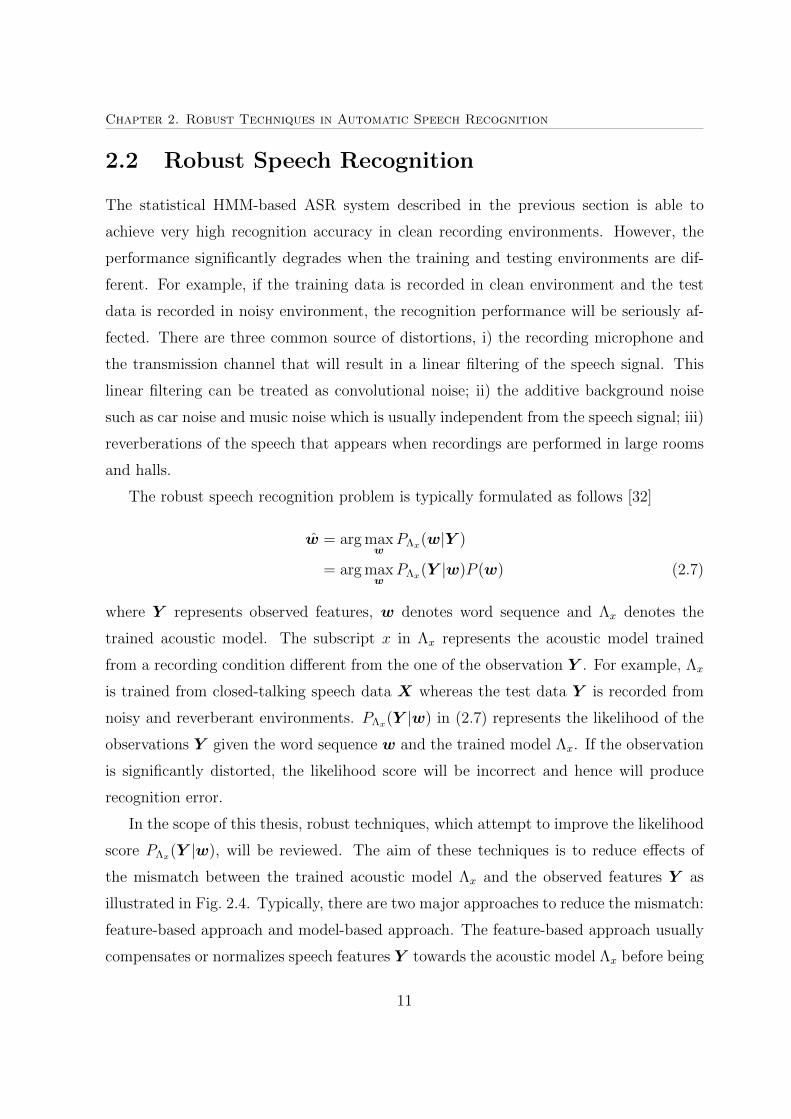
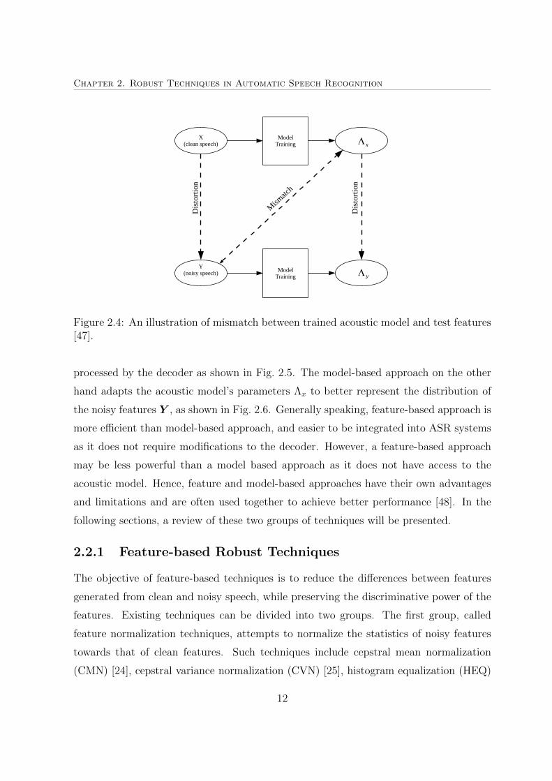
In the scope of this thesis, robust techniques, which attempt to improve the likelihood
score PΛx(Y |w), will be reviewed. The aim of these techniques is to reduce effects of
the mismatch between the trained acoustic model Λx and the observed features Y as
illustrated in Fig. 2.4. Typically, there are two major approaches to reduce the mismatch:
feature-based approach and model-based approach. The feature-based approach usually
compensates or normalizes speech features Y towards the acoustic model Λx before being
11
Chapter 2. Robust Techniques in Automatic Speech Recognition
X(clean speech)
Y(noisy speech)
ModelTraining
ModelTraining
Dis
tort
ion
Dis
tort
ion
Mism
atch
Λ x
Λ y
Figure 2.4: An illustration of mismatch between trained acoustic model and test features[47].
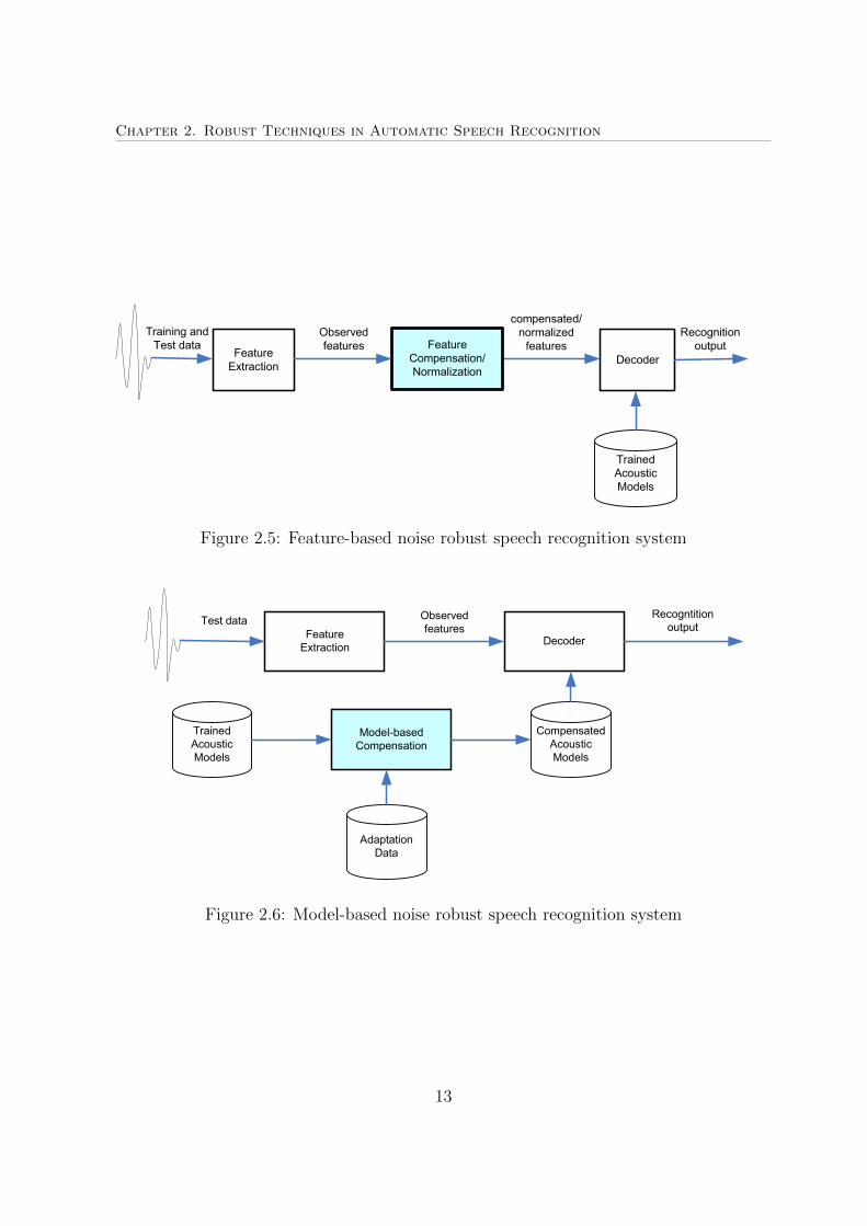
processed by the decoder as shown in Fig. 2.5. The model-based approach on the other
hand adapts the acoustic model’s parameters Λx to better represent the distribution of
the noisy features Y , as shown in Fig. 2.6. Generally speaking, feature-based approach is
more efficient than model-based approach, and easier to be integrated into ASR systems
as it does not require modifications to the decoder. However, a feature-based approach
may be less powerful than a model based approach as it does not have access to the
acoustic model. Hence, feature and model-based approaches have their own advantages
and limitations and are often used together to achieve better performance [48]. In the
following sections, a review of these two groups of techniques will be presented.
2.2.1 Feature-based Robust Techniques
The objective of feature-based techniques is to reduce the differences between features
generated from clean and noisy speech, while preserving the discriminative power of the
features. Existing techniques can be divided into two groups. The first group, called
feature normalization techniques, attempts to normalize the statistics of noisy features
towards that of clean features. Such techniques include cepstral mean normalization
(CMN) [24], cepstral variance normalization (CVN) [25], histogram equalization (HEQ)
12
Chapter 2. Robust Techniques in Automatic Speech Recognition
Feature
ExtractionDecoder
compensated/
normalized
features
Training and
Test dataRecognition
outputFeature
Compensation/
Normalization
Observed
features
Trained
Acoustic
Models
Figure 2.5: Feature-based noise robust speech recognition system
Feature
ExtractionDecoder
Observed
featuresTest data
Recogntition
output
Compensated
Acoustic
Models
Trained
Acoustic
Models
Model-based
Compensation
Adaptation
Data
Figure 2.6: Model-based noise robust speech recognition system
13
Chapter 2. Robust Techniques in Automatic Speech Recognition
[49], relative spectra (RASTA) [27], auto-regressive moving average (ARMA) [50] and
temporal spectral normalization (TSN) [47]. The second group of techniques are called
feature compensation methods and they aim to estimate the underlying clean features
from the observed noisy features, e.g. the spectral subtraction (SS) [13] and MMSE
estimation of short time Fourier amplitude of clean speech [15, 16]. These methods are
briefly introduced in the following subsections.
2.2.1.1 Feature Normalization
Feature normalization is a group of techniques that normalise the various aspects of fea-
ture statistics to a common reference, usually the clean features’ statistics. The simplest
feature normalization techniques is the cepstral mean normalization (CMN) [24], which
simply subtracts the features’ mean values in the cepstral domain. The CMN method
can be used to handle convolutional distortion such as microphone mismatch or linear
transmission channel distortion. Since convolutional noise becomes multiplicative in fre-
quency domain and additive in log-Mel and cepstral domain, subtracting the mean from
the features is able to remove convolutional distortions. The advantages of the CMN
method are its simplicity, low computational cost, ease of implementation and the ability
to handle convolutional noise. However, only normalizing the mean of features to zero
is often insufficient to improve the robustness of ASR in more difficult cases, such as
additive noise cases. Hence, CMN is usually combined with other methods to achieve
better performance.
A natural extension of CMN is the cepstral variance normalization (CVN) [25]. While
CMN normalizes features’ means, CVN normalizes the features’ variances to unity to
address additive noise’s effects on ASR. It is well known that the variance of speech
features is scaled differently in cepstral domain caused by the additive noise due to the
logarithm operator in feature extraction process [51]. Hence, normalizing the variances
of both clean and noisy features to unity reduces the distortions caused by the additive
noise. The CMN and CVN are usually used in cascade and referred to as mean and
variance normalization (MVN) method to handle both additive and convolutional noises.
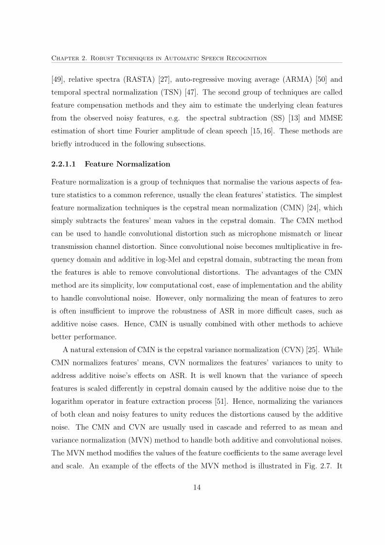
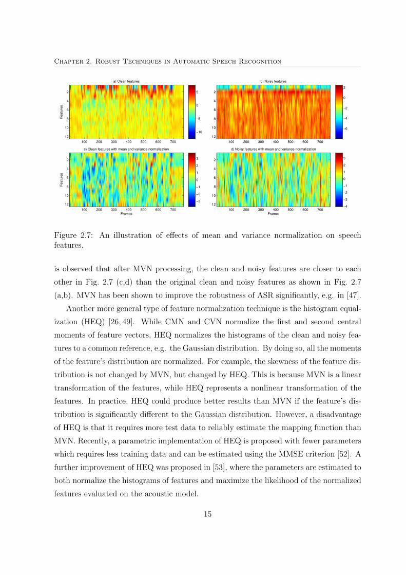
The MVN method modifies the values of the feature coefficients to the same average level
and scale. An example of the effects of the MVN method is illustrated in Fig. 2.7. It
14
Chapter 2. Robust Techniques in Automatic Speech RecognitionF
eatu
res
a) Clean features
100 200 300 400 500 600 700
2
4
6
8
10
12
−10
−5
0
5
b) Noisy features
100 200 300 400 500 600 700
2
4
6
8
10
12
−6
−4
−2
0
2
Frames
Fe
atu
res
c) Clean features with mean and variance normalization
100 200 300 400 500 600 700
2
4
6
8
10
12−3
−2
−1
0
1
2
3
Frames
d) Noisy features with mean and variance normalization
100 200 300 400 500 600 700
2
4
6
8
10
12−4
−3
−2
−1
0
1
2
3
Figure 2.7: An illustration of effects of mean and variance normalization on speechfeatures.
is observed that after MVN processing, the clean and noisy features are closer to each
other in Fig. 2.7 (c,d) than the original clean and noisy features as shown in Fig. 2.7
(a,b). MVN has been shown to improve the robustness of ASR significantly, e.g. in [47].
Another more general type of feature normalization technique is the histogram equal-
ization (HEQ) [26, 49]. While CMN and CVN normalize the first and second central
moments of feature vectors, HEQ normalizes the histograms of the clean and noisy fea-
tures to a common reference, e.g. the Gaussian distribution. By doing so, all the moments
of the feature’s distribution are normalized. For example, the skewness of the feature dis-
tribution is not changed by MVN, but changed by HEQ. This is because MVN is a linear
transformation of the features, while HEQ represents a nonlinear transformation of the
features. In practice, HEQ could produce better results than MVN if the feature’s dis-
tribution is significantly different to the Gaussian distribution. However, a disadvantage
of HEQ is that it requires more test data to reliably estimate the mapping function than
MVN. Recently, a parametric implementation of HEQ is proposed with fewer parameters
which requires less training data and can be estimated using the MMSE criterion [52]. A
further improvement of HEQ was proposed in [53], where the parameters are estimated to
both normalize the histograms of features and maximize the likelihood of the normalized
features evaluated on the acoustic model.
15
Chapter 2. Robust Techniques in Automatic Speech Recognition
While CMN, CVN, and HEQ all normalise the probability distribution of features, an-
other group of feature normalization methods instead attempts to normalise the temporal
information of the speech features, i.e. the correlation between feature frames. For exam-
ple, Relative Spectra (RASTA) [27] and Auto-Regressive Moving Average (ARMA) [50]
are two temporal filters that operate on the feature trajectories to improve the tempo-
ral characteristics of features. RASTA is a bandpass filter that removes the very low
frequencies (< 1Hz) of feature trajectory called modulation frequency. RASTA also at-
tenuates modulation frequencies above 16Hz as it is found that the high frequencies are
mostly due to noises. Hence, RASTA removes modulation frequencies less relevant to
speech recognition to improve features’ robustness. ARMA filter is similar to RASTA,
except that it only smoothes the features without removing the very low frequencies.
Both ARMA and RASTA are designed offline and kept fixed during feature normaliza-
tion. Although ARMA and RASTA improve the temporal characteristics of features,
they do not explicitly normalize the temporal structure of features. A recent temporal
filter, called temporal structure normalization (TSN) filter [54], was proposed to normal-
ize the temporal structure of noisy feature trajectories, represented by the power spectral
density (PSD) function of the trajectories, to that of clean feature trajectories through
linear filtering. The TSN filter is designed on a per-utterance basis, hence adapts to the
speech signal noisy condition automatically. For example, it is shown that the TSN filter
tends to smooth features more heavily when the SNR level is lower and less if the signal
is cleaner.
The distribution-normalizing methods, such as MVN and HEQ, are usually combined
with temporal filters, such as RASTA, ARMA, and TSN, in an ad-hoc way. It is com-
mon that MVN or HEQ is applied first, followed by temporal filters. Recently, a method
called joint spectral and temporal normalization (JSTN) [55] was proposed to integrate
a generalized version of MVN and TSN in a single framework. It is found that JSTN
performs better than simple cascade of MVN and TSN in both noisy and reverberant
speech recognition. One key contribution of JSTN is to introduce maximum likelihood
(ML) criterion and a reference Gaussian mixture model (GMM) trained from clean fea-
tures to guide the filter design. This idea is further extended in maximum normalised
likelihood linear filtering (MNLLF) [56] where a novel Kullback Leibler (KL) divergence
16
Chapter 2. Robust Techniques in Automatic Speech Recognition
based criteria is used to replace the ML criterion. In [56], MNLLF is shown to outperform
JSTN and TSN in noisy and reverberant speech recognition task Aurora-5.
Recently, in [57], a combination of spectral subtraction and temporal structure nor-
malization was studied in Aurora 2 database. The combination performs better than
both SS or TSN alone. In [58], a filter-based histogram equalization (FHEQ) was pro-
posed to integrate a temporal average (TA) filter with HEQ. FHEQ utilizes the TA filter
to smooth the statistic probability sequence before mapping. In [59], the TA filter is
replaced by a Median filter to reduce the sensitive to high local noise intensities.
2.2.1.2 Feature-based Maximum Likelihood Linear Regression
fMLLR is a vector-based linear feature transformation and defined as follows [4, 29]
y(d)t =
D∑i=1
a(d)i x
(i)t + b(d) (2.8)
or in vector form
yt = Axt + b (2.9)
where xt = [x(1)t , ..., x
(D)t ]T and yt = [y
(1)t , ..., y
(D)t ]T are the observed and processed feature
vectors at frame t, respectively. D is the dimensionality of the feature vectors. a(d)i for
i = 1, ..., D is the dth row vector of the transformation matrix A. b(d) is the dth element
of the offset vector b. Each y(d)t is a linear weighted sum of the observed features x
(d)t in
all dimensions of current frame. Hence, fMLLR utilizes the correlation information (or
regularity) between feature dimensions within a frame.
It is well known that applying fMLLR transform in feature space is equivalent to
applying a global CMLLR in model space (i.e. a single transformation is used in model
adaptation) [4,29]. This property leads to the use of the log-likelihood of observations as
the objective function to estimate fMLLR transform. EM algorithm is used to find the
optimal transform. Particularly, the parameters of fMLLR are estimated by maximising
the following auxiliary function
Q(A,A) = Const.+ T log |A|−T∑t=1
M∑m=1
γt(m)
2(Axt + b− µj)TΣ−1
j (Axt + b− µj) (2.10)
17
Chapter 2. Robust Techniques in Automatic Speech Recognition
where γt(m) represents the posterior probability of the mth component {µm,Σm}, M is
the number of Gaussian components and T is the number of frames. In [29], a closed-
form solution has been derived for the diagonal transformation case. In [4], a row by row
iterative method has been proposed to obtain a solution for the full transformation case.
fMLLR transform has been widely used in speech recognition systems to deal with
nuisance variations of speech features, such as speaker variation, channel and noise vari-
ations. A common characteristics of these variations is that their effect on the features is
usually within one analysis frame, hence fMLLR is able to reduce the variations by using
just 1 frame speech features as input. Given enough adaptation data, e.g. several utter-
ances, fMLLR is effective in reducing the contribution of these variations in the feature
representation. However, for distortions that lasts for longer time, e.g. reverberation
effect may last up to 1s, fMLLR is inherently ineffective due to its use of a single frame
that contains at most 0.1s of speech information when considering the dynamic features.
2.2.1.3 Clean Speech Feature Estimation
Noise Suppression
A popular clean speech signal estimator is spectral subtraction (SS) method [13] which
was originally proposed for speech enhancement rather than robust speech recognition.
The SS method tries to remove noise from noisy signal by subtracting the noise magni-
tude from the noisy magnitude in the frequency domain. The noise magnitude can be
estimated from speech-free frames. A general form for SS is [60]
|Xfi,t|γ = max (|Yfi,t|γ − E(|Nfi,t|)γ, ε) (2.11)
where Yfi,t, Xfi,t and Nfi,t are the noisy, estimated clean and noise Fourier coefficients of
a frequency bin fi at a particular frame t, respectively. E(|Nfi,t|) is the expected value of
the noise spectrum, ε is the noise floor to avoid negative estimate of |Xfi,t|γ, and γ is a
tunable parameter to select the domain in which the subtraction takes place. Magnitude
SS is realised when γ = 1 and the phases of the Fourier coefficients of the speech and
noise are assumed to be identical [13, 60]. Power SS is realised when γ = 2 and the
speech and noise are assumed to be uncorrelated [60]. In literature, several variations
18
Chapter 2. Robust Techniques in Automatic Speech Recognition
of the spectral subtraction method have been proposed. They include non-linear spec-
tral subtraction [61], selective spectral subtraction [62], MMSE spectral subtraction [63]
and multi-band spectral subtraction [64]. A detailed review of the spectral subtraction
algorithm and its variations can be found in [65]. Although SS is efficient in removing
noise, its performance heavily relies on an accurate estimation of noise, which is itself a
challenging task especially in nonstationary noisy environments. In addition, SS does not
remove convolutional noise explicitly. Finally, the above SS operates in the frequency
domain and not on the desired final cepstral domain. It is believed that the domain
of clean speech feature estimator should be as close to the final features as possible to
achieve better robustness [16,66].
Besides SS, a group of MMSE estimators have been proposed to operate in various
stages of feature extraction. Let x denote the clean speech feature we want to estimate in
a certain domain, e.g. the log Mel filterbank domain. The MMSE criterion to estimate
x is to minimizes the expected squared errors between the clean estimate x and x.
Mathematically, it is as follows
x = arg minxE(‖xt − xt‖2 | O;M
)= E (xt | O;M)
=
∫RD
xtp(xt | O;M)dxt (2.12)
where ‖·‖2 denote Euclidean norm, O is the noisy observation, D is the dimension of fea-
ture vectors, andM is the set of free parameters used for enhancement. Various MMSE
estimators have been derived in [15, 16, 51, 66, 67]. In these studies, ASR performances
have been shown to improve. However these estimators require accurate noise estimation
which remains a challenge.
Since it is impossible to completely remove the noise from noisy signal, the uncertainty
of the clean feature estimate can be taken into account during decoding to improve the
robustness of ASR system. A solution is that instead of using a point estimate of the
features, the clean speech posterior, i.e. p(x|y) where x is clean features and y observed
features, is embedded into the form of the likelihood calculation [68]. The clean speech
feature estimate is usually dependent on the noise estimate. If the clean estimate is
modelled by a single Gaussian, then the variance of the clean estimate is a function of
19
Chapter 2. Robust Techniques in Automatic Speech Recognition
the noise variance. As a result, the acoustic model variance needs to be compensated
for the noise variance. Another solution is to utilize the joint clean and noisy feature
distribution which can be estimated using the VTS method [51,69]. The likelihood of the
observed features p(y) can then be derived from the joint p(x,y) to obtain the uncertainty
decoding forms such as in [69]. By including uncertainty handling during decoding has
been shown to significantly improve the ASR performance in noisy environments [69].
These techniques need to update the acoustic model and we will present a brief discussions
on model compensation techniques in the next section.
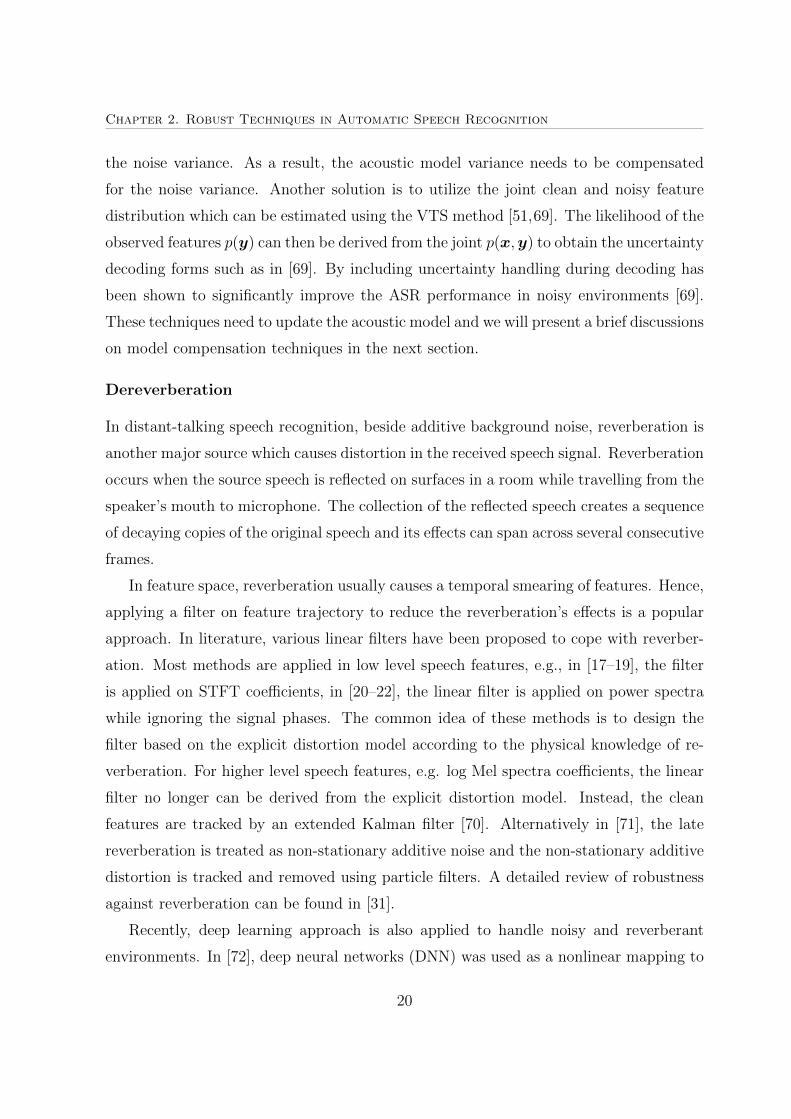
Dereverberation
In distant-talking speech recognition, beside additive background noise, reverberation is
another major source which causes distortion in the received speech signal. Reverberation
occurs when the source speech is reflected on surfaces in a room while travelling from the
speaker’s mouth to microphone. The collection of the reflected speech creates a sequence
of decaying copies of the original speech and its effects can span across several consecutive
frames.
In feature space, reverberation usually causes a temporal smearing of features. Hence,
applying a filter on feature trajectory to reduce the reverberation’s effects is a popular
approach. In literature, various linear filters have been proposed to cope with reverber-
ation. Most methods are applied in low level speech features, e.g., in [17–19], the filter
is applied on STFT coefficients, in [20–22], the linear filter is applied on power spectra
while ignoring the signal phases. The common idea of these methods is to design the
filter based on the explicit distortion model according to the physical knowledge of re-
verberation. For higher level speech features, e.g. log Mel spectra coefficients, the linear
filter no longer can be derived from the explicit distortion model. Instead, the clean
features are tracked by an extended Kalman filter [70]. Alternatively in [71], the late
reverberation is treated as non-stationary additive noise and the non-stationary additive
distortion is tracked and removed using particle filters. A detailed review of robustness
against reverberation can be found in [31].
Recently, deep learning approach is also applied to handle noisy and reverberant
environments. In [72], deep neural networks (DNN) was used as a nonlinear mapping to
20
Chapter 2. Robust Techniques in Automatic Speech Recognition
transform noisy and reverberant speech features to clean features. Another type of neural
network, a denoising autoencoder (DAE), was used in [73,74]. In [75], an improvement of
DEA was proposed by applying a post-processing method based on temporal structure
normalization (TSN) filter on the DEA transformed features to normalize the modulation
spectra of speech features. The combination of DEA and TSN showed a relative error
reduction rate of 9.33% in real reverberant environments.
2.2.1.4 Discussions
In the thesis, three novel feature-based robust techniques will be presented. The first
method [33] is a modification of spectral subtraction [13] for non-stationary noise cases.
This method will be presented in Chapter 3. The second method [34] is a clean speech
feature estimation technique using particle filter and will be presented in Chapter 4. The
third method [36,37] is a general linear feature transformation to map input features to
desired clean training features and will be presented in Chapter 5.
Although these proposed methods are in feature space, their relationships with model-
based approach are high. Particularly, the first method is motivated by a limitation of a
vector Taylor series (VTS) model compensation method. The VTS model compensation
works well for stationary noise condition but performance degrades for non-stationary
noise cases. Hence, the first method proposed to combine spectral subtraction with the
VTS model compensation to improve the ASR system under the non-stationary noisy
condition. The second method uses side information provided by an acoustic model to
estimate the clean speech features. Hence, model adaptation techniques can be applied
to improve the accuracy of the side information. Finally, in the third work, we found
that feature adaptation and model adaptation are complementary and applying them
jointly will significantly improve performance. From these observations, we will review
model-based robust techniques to provide the background knowledge to understand the
relationships in the following sections.
2.2.2 Model-based Robust Techniques
In the mainstream HMM-based ASR systems, the acoustic model captures the condi-
tional distribution of training features given speech classes. When the speech signal is
21
Chapter 2. Robust Techniques in Automatic Speech Recognition
corrupted by channel and noise, the distribution of test features is different from the
training features, i.e. there is mismatch between training and test conditions. As a re-
sult, the acoustic model no longer accurately represents the test features and hence causes
the recognition performance to degrade. To improve robustness, model-based methods
have been proposed to adapt the acoustic model to better represent the test feature’s
distribution. This strategy is different from feature-based approach which transforms
the observed noisy feature towards the training feature while keeping the acoustic model
unchanged.
Model adaptation methods usually require adaptation data and its true transcription
to adapt the acoustic model [30]. It is required that the adaptation data are similar to
the target test data in terms of acoustic characteristics as otherwise, a mismatch again.
Generally speaking, the more adaptation data, the more effective the adaptation. In
cases when there is no adaptation data, multiple pass decoding strategy can be used [30].
In the first pass, the unadapted acoustic model is used to decode the test utterance to
obtain an initial hypothesis. This hypothesis is then treated as the true transcription and
the test data are reused to adapt the model. The adapted model is then used to decode
the test utterance. This strategy of adaptation is called self-adaptation or unsupervised
adaptation [30].
There are several ways to categorize the numerous model adaptation methods in the
literature. For example, one can classify them based on the use of distortion modelling,
e.g. explicit or implicit distortion modellings [32]. In the explicit distortion modelling,
researchers utilize the physical knowledge of how the speech is distorted to predict the
noisy acoustic model from the clean acoustic model. In the implicit distortion modelling
case, a model transformation which does not rely on the physical knowledge is applied.
In this section, the implicit distortion modelling approach is first reviewed, followed
by explicit distortion modelling. Besides describing the methods, their advantages and
disadvantages will be discussed.
2.2.2.1 Implicit Distortion Modelling Approach
Maximum a posteriori Adaptation
The classical model adaptation method is the maximum a posteriori [3] method that was
initially proposed for speaker adaptation but is also applicable to mismatch caused by
22
Chapter 2. Robust Techniques in Automatic Speech Recognition
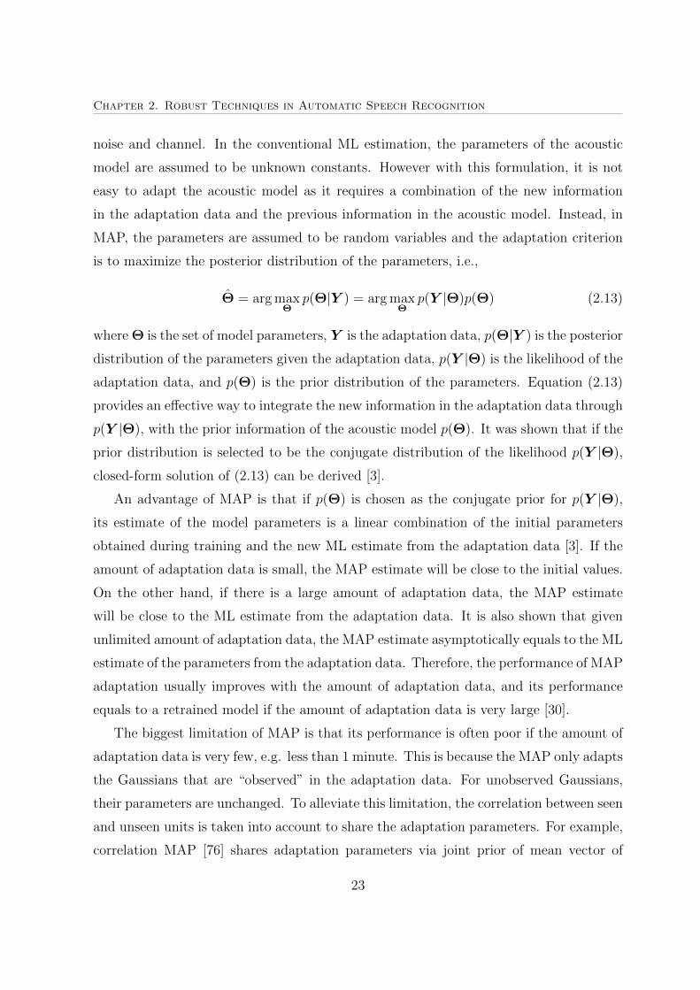
noise and channel. In the conventional ML estimation, the parameters of the acoustic
model are assumed to be unknown constants. However with this formulation, it is not
easy to adapt the acoustic model as it requires a combination of the new information
in the adaptation data and the previous information in the acoustic model. Instead, in
MAP, the parameters are assumed to be random variables and the adaptation criterion
is to maximize the posterior distribution of the parameters, i.e.,
Θ = arg maxΘ
p(Θ|Y ) = arg maxΘ
p(Y |Θ)p(Θ) (2.13)
where Θ is the set of model parameters, Y is the adaptation data, p(Θ|Y ) is the posterior
distribution of the parameters given the adaptation data, p(Y |Θ) is the likelihood of the
adaptation data, and p(Θ) is the prior distribution of the parameters. Equation (2.13)
provides an effective way to integrate the new information in the adaptation data through
p(Y |Θ), with the prior information of the acoustic model p(Θ). It was shown that if the
prior distribution is selected to be the conjugate distribution of the likelihood p(Y |Θ),
closed-form solution of (2.13) can be derived [3].
An advantage of MAP is that if p(Θ) is chosen as the conjugate prior for p(Y |Θ),
its estimate of the model parameters is a linear combination of the initial parameters
obtained during training and the new ML estimate from the adaptation data [3]. If the
amount of adaptation data is small, the MAP estimate will be close to the initial values.
On the other hand, if there is a large amount of adaptation data, the MAP estimate
will be close to the ML estimate from the adaptation data. It is also shown that given
unlimited amount of adaptation data, the MAP estimate asymptotically equals to the ML
estimate of the parameters from the adaptation data. Therefore, the performance of MAP
adaptation usually improves with the amount of adaptation data, and its performance
equals to a retrained model if the amount of adaptation data is very large [30].
The biggest limitation of MAP is that its performance is often poor if the amount of
adaptation data is very few, e.g. less than 1 minute. This is because the MAP only adapts
the Gaussians that are “observed” in the adaptation data. For unobserved Gaussians,
their parameters are unchanged. To alleviate this limitation, the correlation between seen
and unseen units is taken into account to share the adaptation parameters. For example,
correlation MAP [76] shares adaptation parameters via joint prior of mean vector of
23
Chapter 2. Robust Techniques in Automatic Speech Recognition
correlated units. Alternatively, the correlation among Gaussians can be organized as a
tree structure such as in structured MAP [77]. A transformation is assigned to each
node of the tree and estimated using MAP scheme. Hence, if little adaptation data is
available, the transformation parameters of the leaf nodes close to the prior and if more
adaptation data are available, the prior transformation parameters can be inherited from
higher levels in the tree.
Transform-based Adaptation
Linear transformation of model parameters is a popular approach to adapt the acoustic
model. Examples include the maximum likelihood linear regression (MLLR) [5, 78] and
constrained MLLR (CMLLR) [4] approaches. In MLLR, it is assumed that the mean
vector and covariance matrix of the adapted model are linear transformations of the
initial model as follows:
µm = Aµm + b
Σm = HΣmHT (2.14)
where µm and Σm are the adapted mean and covariance matrix of the mth Gaussian
mixture in the acoustic model, A is a D×D transform matrix for mean vectors, b is a D
dimensional bias vector, H is a D×D transformation matrix for the covariance matrix,
and D is the feature vector dimension. A, H and b are estimated by maximizing the
likelihood of the adaptation data Y as follows:
{A, b, H} = arg maxA,b,H
log p(Y |Θ,A, b,H) (2.15)
As there is no closed-form solution for the above maximization problem, the expectation
maximization (EM) method is usually used to find the solution iteratively [4, 5].
An advantage of MLLR adaptation compared to MAP is that it is less affected by the
unseen Gaussians discussed in the previous section. This is due to the fact that the mean
and covariance transforms are shared by all the Gaussians in the acoustic model, and
hence the mean and covariance of unseen Gaussians are also adapted through the shared
transforms. However, as the amount of adaptation data increases, the performance gain
of MLLR quickly saturates as the number of free parameters in the transforms is limited.
24
Chapter 2. Robust Techniques in Automatic Speech Recognition
To increase the effectiveness of the MLLR, multiple sets of transforms can be used instead
of a single set of global transforms. To achieve this, the Gaussians in the acoustic model
are usually clustered into several classes using regression-tree-based clustering [5], and
then the transformation parameters are estimated for each data class. The number of
classes is usually proportional to the amount of adaptation data to ensure that there is
enough data for each class. In addition, MLLR has been found to be complementary to
MAP and these two methods can be applied together [8, 79,80].
The MLLR adaptation method will modify all the acoustic model parameters in its
adaptation process. This will be computationally expensive if the model is large. The
constrained version of MLLR, i.e. the CMLLR adaptation, reduces the computation
significantly by applying feature transformation to achieve the same effects instead. CM-
LLR differs from MLLR by the fact that the mean and the covariance transforms are
constrained to be the same; in other words, H = A. With this constraint, it is shown
in [4] that transforming the model parameters is equivalent to the transformation of
feature vectors. In the case of multiple classes of transforms, the feature vectors are simi-
larly transformed multiple times using class-dependent transforms. As feature transform
is much more efficient than transforming the models, especially when model need to be
updated constantly, CMLLR provides an efficient way to adapt the model towards the
test environment.
Although MLLR and CMLLR can achieve faster adaptation than MAP, they still
requires a sufficient amount of adaptation data to reliably estimate the transform pa-
rameters [81]. In the case when there are few adaptation data, MLLR and CMLLR often
fail. In such cases, there are several ways to improve MLLR and CMLLR. The simplest
way is to constrain the transform matrices to be diagonal or block diagonal to reduce the
amount of free parameters. However, this method often seriously limits the performance
gain of model transformation. Another approach is to use Bayesian estimate of trans-
forms rather than ML estimate as in MLLR and CMLLR. In such methods, the concept
of MAP and transform-based adaptation are combined and a prior distribution for the
transform parameters is introduced, again conjugate prior is chosen for simplicity [82]. A
similar approach to Bayesian estimate is to regularize the ML estimation of transform es-
timation. For example, L1 and L2 constraints are added into the ML estimation formula
to regularize the ML estimate [83,84].
25
Chapter 2. Robust Techniques in Automatic Speech Recognition
Model Combination Methods
An even faster way for model adaptation is to linearly combine multiple existing models
[85,86] or transforms [87]. In such methods, a group of acoustic models or transforms are
first trained for a specific speaker or environment. The trained models and transforms
are called basis models and transforms, respectively. During adaptation, it is assumed
that the adapted model or transform can be approximated by a linear combination of
these basis models or transforms. The advantage of this approach is that only the weights
of the individual models or transforms need to be estimated, which is usually much less
than the number of free parameters in the acoustic model or transform. Hence, very
little adaptation is required to estimate these weighting parameters.
Many of the model combination methods estimate the mean vectors of the adapted
model as a combination of the mean vectors of the speaker and environment dependent
basis models, e.g. cluster adaptive training (CAT) [85]. In these methods, the mean of
the adapted model is estimated as follows:
µm =N∑i=1
wiµim (2.16)
where µim is the mean vector of the mth Gaussian of the ith basis model, wi is the weight
of the ith basis model and shared by all the Gaussians, and N is the total number of basis
models. Similar to MLLR, the weights are estimated by maximizing the log likelihood of
the adaptation data, log p(Y |Θ, w1, ..., wN), and closed-form solution is available.
In another mean combination method, called eigenvoice [86], the mean vectors of a
basis model are concatenated to form a supervector for the basic model. The principal
component of supervectors for all the basis models are then found using FA. During
adaptation, the mean supervector of the adapted model is found by a linear combination
of the principal components of supervector. By this strategy, the correlation between the
mean vectors of different basis models are captured and hence only very few number of
principal components are needed for the linear combination.
While CAT and eigenvoice combine basis models to form the adapted model, another
class of approach, the transform combination methods instead form a new transform
for specific adaptation data by linearly combining the basic transforms. Two examples
26
Chapter 2. Robust Techniques in Automatic Speech Recognition
are the mean MLLR transform combination [88] and eigenMLLR [87]. In the mean
MLLR transform combination, the mean basis transforms are directly used in the linear
combination, while in eigenMLLR, the principal components of the transforms are used.
The concept of eigenMLLR is very similar to eigenvoice, i.e. to find a few number of
principal components to reduce the number of basis needed for the linear combination. In
eigenMLLR, each basis transforms is first converted to a vector form, then the principal
components of the vectors of all basis transforms are found using PCA. Both mean
transform combination and eigenMLLR are found to adapt the models efficiently with
just several seconds of adaptation data.
Though model combination methods improve ASR performance when given small
adaptation data, the word accuracy quickly saturates when given more adaptation data.
This is due to the fact that only a very small number of adaptation parameters are
available for optimization [89]. One solution to this issue is to apply this approach as
global adaptation and then use the global adapted models as a prior information for
MAP adaptation [89].
2.2.2.2 Explicit Distortion Modelling Approach
The previous section discussed model-based methods which do not directly utilize a
physical model of noise distortion. Such techniques are referred to as adaptive model-
based methods [90]. This section discusses another group of model-based methods which
make use of a physical model of noise distortion to predict the noisy acoustic model.
Such techniques are referred to as predictive model compensation [90].
Distortion Modelling
Speech signals are corrupted by additive noises and channel distortions according to
physical laws and the corruption process can be described mathematically. For example,
a simple equation to describe the relationship between speech, noise, and channel in the
time domain is as follows [91]:
y[m] = x[m] ? h[m] + n[m] (2.17)
where x[m] is the unobservable clean speech signal, h[m] is channel impulse response,
n[m] is the additive noise, and y[m] is the observed corrupted speech signal. m is the
27
Chapter 2. Robust Techniques in Automatic Speech Recognition
time domain sample index and ? is the convolution operator. Although there are other
possible equations to describe the noise corruption process, the equation (2.17) is found
to be adequate for speech recognition and popular in robust speech recognition literature
[51, 90–92]. From (2.17), it is possible to derive the relationship between the clean and
noisy features, usually called mismatch function. If the distribution of clean speech
features, noise features, and channel features are all known, it is theoretically possible
to predict the exact distribution of noisy features. This fact motivates all predictive
model-based methods, in which the task is to find an acoustic model that models the
distribution of the noisy test data well. Predictive model compensation methods [90]
usually first estimate the noise and channel statistics from the adaptation data, and then
estimate the noisy acoustic model from the clean trained acoustic model through the
mismatch function.
Due to its use of the distortion model, predictive methods have some advantages
over adaptive model-based methods discussed in the previous section. One important
advantage is that the predictive methods usually have only a small number of parameters
to estimate, and hence require less adaptation data. For example, the free parameters
to be estimated are the noise and channel statistics, which are usually represented by
Gaussian distributions. This is usually less than adaptive model-based methods in which
the free parameters are the acoustic model parameters itself (e.g. MAP) or transform
parameters (e.g. MLLR). Although the number of free parameters can also be reduced by
some tying, such parameter tying usually results in limiting transformation of the acoustic
model and reduces the potential gain from model adaptation [81]. On the other hand,
predictive model compensation is able to apply different transformation to individual
Gaussians in the acoustic model [90], even though the noise and channel distributions
are shared among all the clean features Gaussians. This is due to the fact that the
knowledge of interactions among the clean speech, noise, and channel is explicitly used
in predictive methods through the mismatch function.
The Mismatch Function
From the distortion model (2.17) given in time domain, we need to obtain the mismatch
function in the feature domain. According to [11], the mismatch function in the MFCC
28
Chapter 2. Robust Techniques in Automatic Speech Recognition
domain is:
y = C log
(exp(C−1(x+ h)) + exp(C−1(n)) + 2α · exp(
1
2C−1(x+ h+ n))
)= f(x,h,n) (2.18)
where y, x, n, and h are the noisy, clean, additive noise feature vectors, and convolutional
distortion in the MFCC domain, respectively. Note that we ignored the frame index for
simplicity. C and C−1 are the DCT matrix and its pseudo inverse. The logarithm log()
and exponential exp() functions in (2.18) are element-wise operations and the · operation
for two vectors denotes element-wise product. α is the “phase factor” proposed in [66]
and usually set to a constant for simplicity. f(x,h,n) is referred to the phase-sensitive
mismatch function. Magnitude phase-insensitive mismatch function results from α = 1
and power phase-insensitive mismatch function as α = 0 [92]. For the dynamic features,
the continuous time approximation is commonly used to derive the dynamic parameter
mismatch function (for details of derivation, see [11]).
It is observed that the static parameter mismatch function, i.e. equation (2.18), is
highly nonlinear. As a result, it is very difficult to predict the distribution of the noisy
features given the distributions of clean features, noise, and channel in the feature domain.
Various approximation methods have been proposed and are reviewed as follows.
Approximations of the Noisy feature Distribution
The predictive model compensation approach is usually applied for the HMM with GMM
as acoustic model. For each HMM state of the acoustic model, a noisy GMM is predicted
from the original clean trained GMM. For simplicity, it is usually assumed that each
mixture of the noisy GMM is individually estimated from clean trained mixture GMM.
With this assumption, the noisy model prediction problem can be described as follows:
for each clean Gaussian in the acoustic model, a noisy Gaussian is generated by combining
the clean Gaussian with the noise and channel Gaussians. For example, the noisy feature
mean µ(s,m)y of the mth Gaussian mixture of the sth state is defined as
µ(s,m)y = E(f(x,h,n)|s,m) (2.19)
29
Chapter 2. Robust Techniques in Automatic Speech Recognition
where E is the expectation operator and f is the mismatch function. As the mismatch
function f(x,h,n) is highly non-linear, there is no closed-form solution for the integral.
Various methods have been proposed to evaluate (2.19) efficiently.
In [93], numerical integration and Monte-Carlo sampling approaches have been used
to evaluate the integral. In the numerical integration approach, the Gauss-Hermite
quadrature [94] has been used to approximate the integrals in order to reduce the com-
putational cost. In the Monte-Carlo sampling approach, clean feature samples and noise
feature samples are generated following their distributions and noisy feature samples are
then computed through the mismatch function. The noisy feature distribution can then
be estimated from these noisy feature samples. By increasing the number of samples,
very accurate estimates of the noisy model parameters can be achieved. However, as the
total number of samples increases, the computational cost increases dramatically [90].
To obtain a closed-form solution of equation (2.19), another approach, called log-
normal approximation, was applied in the parallel model combination (PMC) framework
[93]. In PMC, noise and clean speech models are first converted from the cepstral feature
domain to the filterbank domain (before logarithm and DCT). As the features and noises
are assumed to be Gaussian distributed, their counterparts in the filterbank domain are
log-normal distributed. The advantage of generating noisy models in filterbank domain is
that the mismatch function in the filterbank domain can be approximated as y = x+ n,
i.e. the noisy filterbank coefficients is just the addition of the clean speech and noise
filterbank coefficients. However, the distribution of y is unknown due to log-normal
distributions of x and n. Therefore, the log-normal approximation is used for simplicity
which states that the sum of two log-normally distributed variables is approximately
log-normally distributed. By assuming that y also follows log-normal distribution, the
conversion back to cepstral domain of the noisy model parameters is straightforward as
the noisy features will be normally distributed in the cepstral domain.
The PMC is an effective framework utilizing the physical knowledge reflecting the
impact of noise on speech to compensate the acoustic models. The key idea is that the
speech features are converted to a suitable feature domain to more easily estimate the
noisy distribution. Although the log-normal approximation can be applied efficiently in
filter-bank domain, it does not provide an easy way to obtain a closed-form solution of
30
Chapter 2. Robust Techniques in Automatic Speech Recognition
acoustic model compensation in cepstral domain and thus is hard to combine with other
optimization methods, e.g. ML noise parameters re-estimation.
Another way to predict the noisy feature distribution efficiently is to use the vector
Taylor series (VTS) expansions to approximate the mismatch function (2.18). If the
zeroth-order VTS expansion is used and the channel and the phase factor are ignored,
the estimate of the noisy mean is obtained as
µy ' C log(exp(C−1µx) + exp(C−1µn)) (2.20)
where µy and µx are feature means of noisy and clean Gaussian mixtures of speech
model; µn is the feature mean of noise model. This approximation is also referred to as
the log-add approximation in [93]. Although it provides a simple way to update the mean
vectors, the disadvantage of using zeroth-order VTS approximation is that the variance
of the Gaussians can not be updated.
If the first-order VTS expansion is used, the mismatch function (2.18) becomes a
linear function as follow [11]
y ' f(µx,µh,µn) + Jx(x− µx) + Jh(h− µh) + Jn(n− µn) (2.21)
where f(µx,µh,µn) is the value of the mismatch function evaluated at the expansion
point (µx,µn,µh). The Jacobian matrix J(·) is defined as the partial differentiation
of the mismatch function w.r.t. each variable and evaluated at the expansion point
(µx,µn,µh), i.e.
J(·) =∂y
∂(·)
∣∣∣∣µx,µn,µh
(2.22)
The first-order VTS expansion approximates the highly non-linear mismatch function
(2.18) by the Gaussian-dependent piecewise linear function (2.21). As there are a large
number of Gaussian in the acoustic model, the mismatch function is approximated by a
large number of linear function.
Since (2.21) is a linear function w.r.t. x, h and n, it significantly simplifies the esti-
mation of noisy distribution. Particularly, the noisy distribution’s mean and covariance
are computed as follows [11]
µy = f(µx,µh,µn) (2.23)
Σy = JxΣxJtx + JnΣnJ
tn (2.24)
31
Chapter 2. Robust Techniques in Automatic Speech Recognition
From the above equations, it shows that the first-order VTS approximation allows the
update of the covariance matrix to reflect the effects of noise. This is in contrast with
the zeroth-order VTS in which the covariance matrix cannot be updated.
The above discussed approximations have their own advantages and disadvantages.
The log-add approximation in equation (2.20) is the simplest but ignores variance com-
pensation. The log-normal approximation and first-order VTS can be used to compensate
the variances but are computationally expensive. In addition, the noisy covariance ma-
trix is usually full rank even though the clean model covariance matrix is diagonal. To
enable fast decoding, it is common to diagonalize the noisy covariance [92]. Currently,
the first-order VTS is popular due to its linearisation of mismatch function. This lineari-
sation simplifies the noisy model parameter estimation and provides an effective way to
estimate the noise model parameters which is hard in the PMC approach.
The first-order VTS model compensation also motivated the first work in this the-
sis. In VTS, the noise features are usually assumed normally distributed, although this
assumption is not true in real-life condition. Hence, the first work proposes a feature
enhancement process to normalize the statistics of the noise features toward a Gaussian
distribution. It helps to improve the accuracy of the noise model estimation, and hence
improve the accuracy of word recognition.
Noise Model Parameter Estimation
To complete the review of predictive model compensation, the estimation of noise and
channel will be discussed. The additive noise is usually modelled by a single Gaussian
distribution with a mean vector and covariance matrix. The channel is however assumed
to be constant and hence only the mean vector is estimated. A simple method is to
compute the mean and covariance matrix of noise feature vectors from the speech-free
frames and the convolutional noise mean is set to zero. The noise and channel statistics
are optimized by using the maximum likelihood (ML) criterion, i.e. seeking for a set of
noise parameters that maximizes the likelihood of the noisy speech features evaluated on
the compensated noisy acoustic model [11,95].
An advantage of the ML noise estimation is that the decoder’s feedback is taken
into account to optimize the noise model parameters. Although the estimated noise and
32
Chapter 2. Robust Techniques in Automatic Speech Recognition
channel may not be the true additive noise and channel, they are expected to work well
for the ASR task as it is optimized for this purpose [92]. A disadvantage of the ML
noise estimation is its high computational cost due to the multiple decoding passes for
obtaining the decoder’s feedback.
2.3 Chapter Summary
In this chapter, the feature-based and model-based robust ASR techniques are reviewed.
These two approaches have their own advantages and disadvantages. For example, the
feature-based methods are easy to implement and computationally efficient, while the
model-based methods are more powerful and flexible but generally requires more com-
putational power. In practice, these two groups of techniques can be used together to
improve ASR robustness. For example, both feature normalization (e.g. MVN) and
model adaptation (e.g. MLLR/CMLLR) are used in many practical systems.
In Chapter 3, a novel combination of spectral subtraction method and VTS model
compensation will be proposed. The spectral subtraction method will be modified to only
reduce the non-stationary characteristics of the noise while the VTS model compensation
will be used to handle the residual noise.
In Chapter 4, a novel approach using side information from HMM into particle filter
framework to track the clean speech features will be presented. This is a novel approach
to integrate the distortion model of speech into the decoding process.
In Chapter 5, a generalized linear feature transformation to compensate for the back-
ground noise and reverberation will be presented. The transform is the generalization of
fMLLR transform and trajectory-based transform. It is motivated by the finding that
human speech comprehension relies on the integrity of both the spectral content and
temporal envelope of speech signal.
33
Chapter 3
Combination of FeatureEnhancement and VTS ModelCompensation for Non-stationaryNoisy Environments
One of the main causes of speech distortion is due to background noise. Normally,
the background noise is assumed to be stationary. However in real-life, the stationary
assumption is false as most noises such as babble noise exhibit some degree of non-
stationary characteristics. Nevertheless, by assuming stationarity, one greatly simplifies
the complexity of robust methods such as in VTS model compensation [96]. Motivated
by the efficiency of the stationary assumption, a novel feature enhancement is proposed
to normalise the background noise so that the assumption becomes more accurate.
The proposed method is a modification of spectral subtraction (SS) method [13].
Instead of trying to completely remove the noise from noisy speech, the proposed method
only tries to make the noise feature statistics more stationary. By this strategy, it reduces
the difficulty of both the enhancement problem as well as the back-end process. If we
attempt to completely remove the noise in the front-end process, it may cause the loss of
speech information in the speech data. Consequently, it will make the back-end process
harder to correctly estimate the phone sequence. In our approach, we try to remove only
a portion of the noise where the noise level is high, and add some noise to the input signal
where the noise level is low. In this way, the residual noise can be made more stationary
and be effectively handled in the back-end process using VTS model compensation.
34
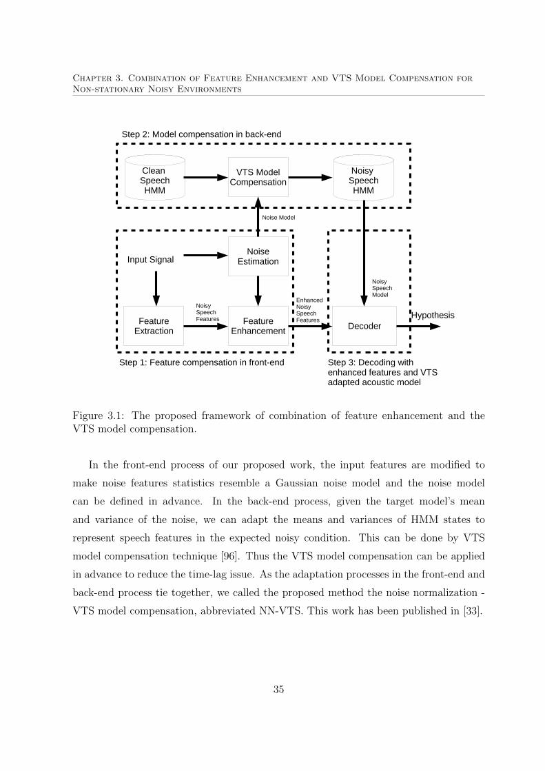
Chapter 3. Combination of Feature Enhancement and VTS Model Compensation forNon-stationary Noisy Environments
Input Signal
FeatureExtraction
FeatureEnhancement
NoiseEstimation
Clean SpeechHMM
VTS ModelCompensation
Noisy SpeechHMM
Decoder
Noise Model
Hypothesis
NoisySpeechModel
EnhancedNoisySpeechFeatures
NoisySpeechFeatures
Step 2: Model compensation in back-end
Step 1: Feature compensation in front-end Step 3: Decoding with enhanced features and VTS adapted acoustic model
Figure 3.1: The proposed framework of combination of feature enhancement and theVTS model compensation.
In the front-end process of our proposed work, the input features are modified to
make noise features statistics resemble a Gaussian noise model and the noise model
can be defined in advance. In the back-end process, given the target model’s mean
and variance of the noise, we can adapt the means and variances of HMM states to
represent speech features in the expected noisy condition. This can be done by VTS
model compensation technique [96]. Thus the VTS model compensation can be applied
in advance to reduce the time-lag issue. As the adaptation processes in the front-end and
back-end process tie together, we called the proposed method the noise normalization -
VTS model compensation, abbreviated NN-VTS. This work has been published in [33].
35
Chapter 3. Combination of Feature Enhancement and VTS Model Compensation forNon-stationary Noisy Environments
3.1 Overview of the Proposed Framework
The proposed framework is illustrated in Figure 3.1. First, the noise information (n1:T ,µn,Σn)
are estimated from the noisy speech input signal, where n1:T represents noise estimate
for frames 1 to T , and µn and Σn are the mean and diagonal covariance matrix of
n1:T . With the estimated noise information, the noisy speech features are processed to
reduce the non-stationary characteristics of the noise. Note that this process does not
try to estimate the clean speech features but only to modify the features such that the
noise becomes more stationary and can be better represented by a single Gaussian noise
model. The residual noise will be handled in back-end process using the VTS model
compensation.
There are 3 problems in the framework. The first problem is how to enhance the
features such that the residual noise is more stationary. The second problem is how to
handle the residual noise using VTS model compensation. The third problem is how
to estimate the noise in each frame. In this work, enhancing the features to normalize
the noise statistics (the first problem) is emphasized. Handling the remaining noise (the
second problem) is based on VTS model compensation in [96]. In this study, we will first
use the ground truth noise magnitude (the third problem) to examine the feasibility and
performance of the proposed work under ideal noise estimate condition first.
A key question for this work is: if the ground truth noise magnitudes is available,
would applying the proposed noise normalization be better than applying noise subtrac-
tion technique? The answer is yes (more details are presented later). With only noise
magnitude information, we are still unable to estimate exactly the clean speech due to
the unknown phase information between speech and noise. Hence by attempting to com-
pletely remove noise, it may result in loss of speech information and thus make it harder
for the speech recognition step later. By proposing noise normalization method which
allows us to control noise levels and strive to retain all the speech information, the VTS
model compensation in the second stage would be less affected.
The actual motivation of this work is from the VTS model compensation. The VTS
method requires a noise model to estimate a noisy speech model from the clean speech
model. Since the VTS method usually works well with a Gaussian noise model, it is not
optimal if the noise is non-stationary. Therefore, the aim of this work is to reduce the
36
Chapter 3. Combination of Feature Enhancement and VTS Model Compensation forNon-stationary Noisy Environments
non-stationary characteristics of the noise so that the VTS method can work better in
non-stationary noisy environments.
In our framework, both front-end and back-end phases are addressed to handle the
non-stationary noise. The noise normalization in the front-end phase is first presented.
Handling the residual noise by using the VTS model compensation in the back-end phase
is then derived.
3.2 Feature Enhancement
The objective of the feature processing stage is to process the features such that the
residual noise in the processed features is more stationary than the original noise. Specif-
ically, if the original noise has mean µn and variance Σn, then the process attempts to
make the residual noise to have the same mean µn, but with a smaller variance.
Given that nt for t = 1, ..., T is the noise in a test utterance in the MFCC domain
and T is the number of frames, a Gaussian distribution N (µn,Σn) can be estimated. To
reduce the noise of the features, we modify the approach of [13,60] such that the features
at time t are processed as follows
yt = C log[max{exp(C−1yt)− exp(C−1nt) + exp(C−1µn), ε}
](3.1)
where yt and yt denote the processed features and the original noisy features, respectively,
C and C−1 are the DCT and inverse DCT matrices, the log and exp functions are
element-wise operators and ε is the noise floor. The operation exp(C−1yt) converts yt
from MFCC domain to Mel filterbank domain. Similarly, exp(C−1nt) and exp(C−1µn)
convert the noise and noise mean to the Mel filterbank domain. It is assumed that
the noisy filterbank is the sum of the clean and noise filterbanks, i.e. exp(C−1yt) =
exp(C−1xt)+exp(C−1nt). Hence, the nonstationary noise can be removed by subtracting
it from the noise filterbank. This is the same as applying spectral subtraction in the
filterbank domain. As spectral subtraction may result in negative filterbank coefficients,
a noise floor ε is used to guarantee positive filterbank coefficients. However, the noise
floor introduces a nonlinear distortion to the features. Instead, we propose to add the
global noise µn back to the processed features. This is different from existing works
37
Chapter 3. Combination of Feature Enhancement and VTS Model Compensation forNon-stationary Noisy Environments
of [13,60] which do not have the use of including exp(C−1µn). As a result, the chance of
the processed noisy filterbanks being negative is significantly reduced. In addition, the
residual noise in the processed features becomes similar to the global noise µn and can
be handled in the VTS model compensation.
In equation (3.1), the instantaneous noise is completely removed in the processed fea-
tures. In practice, as the estimated noise may not be accurate and the phase information
between speech and noise is unknown, removing the estimated noise from the features
may introduce significant distortions. Hence, a partial removal of the instantaneous noise
by the use of weighting α is used instead:
yt = C log[max{exp(C−1yt)− α exp(C−1nt) + α exp(C−1n), ε}
](3.2)
where n and nt are the estimated global noise and local noise feature vectors, respectively.
To generalize the global noise variable in (3.2), we use n to denote the global noise
estimate. The global noise represents the estimated noise in entire utterance whereas
local noise represents estimated noise at a particular time t. α is the tunable parameter
in range 0 to 1 to control the degree of removing the local noise.
3.3 Relationship Between Clean and Enhanced Fea-
tures
Different from noise reduction approach [13] where the standard approach is to completely
remove the noise from noisy speech, our strategy is to have the enhanced features as in
(3.2) still noisy, but with its non-stationary characteristic reduced. By limiting the noise
reduction, this enhancement approach reduces the loss of speech information as well as
simplifying the modelling of noise in the back-end VTS module.
The relationship between clean features and enhanced features can be modelled by a
mismatch function. Using the phase-insensitive mismatch function [32] to represent the
relationship between noisy feature yt, clean feature xt and the local noise nt, i.e.
yt ' C log(exp(C−1xt) + exp(C−1nt)
)(3.3)
38
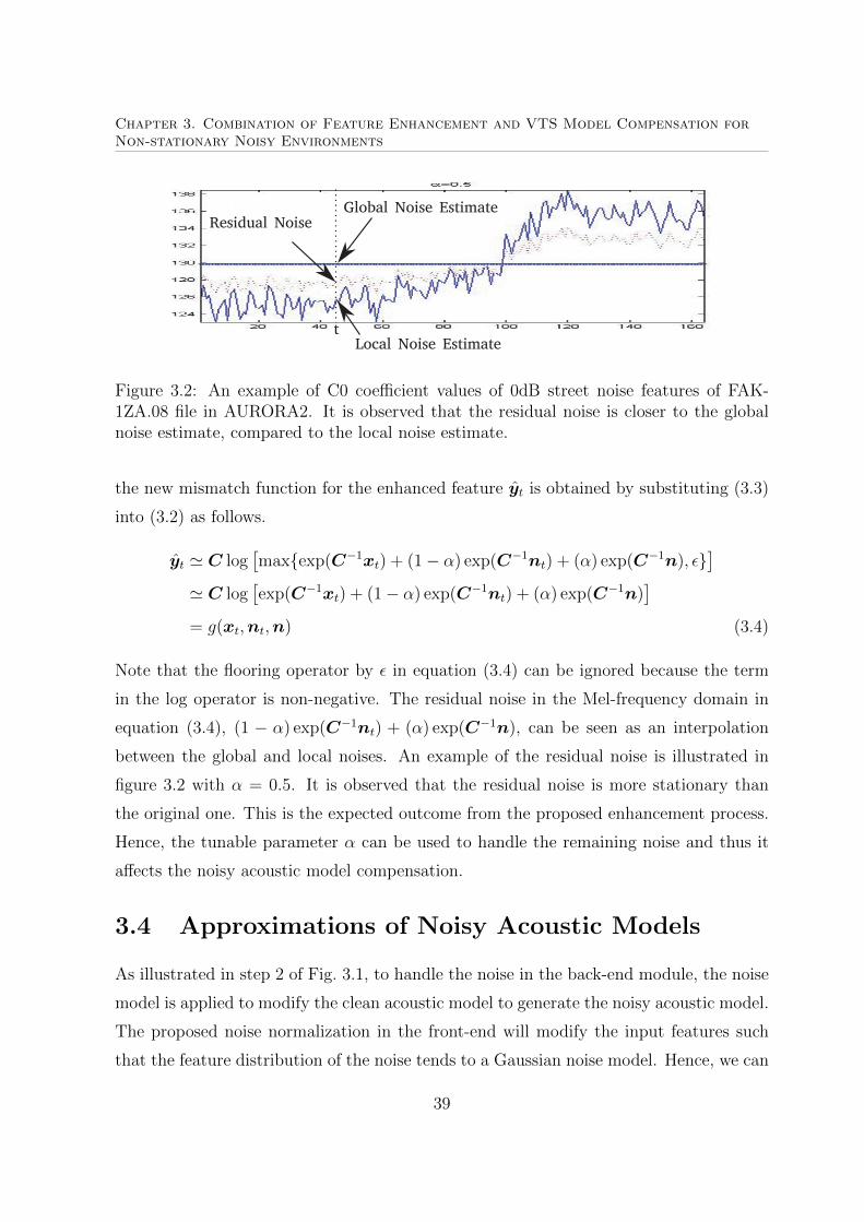
Chapter 3. Combination of Feature Enhancement and VTS Model Compensation forNon-stationary Noisy Environments
Figure 3.2: An example of C0 coefficient values of 0dB street noise features of FAK-1ZA.08 file in AURORA2. It is observed that the residual noise is closer to the globalnoise estimate, compared to the local noise estimate.
the new mismatch function for the enhanced feature yt is obtained by substituting (3.3)
into (3.2) as follows.
yt ' C log[max{exp(C−1xt) + (1− α) exp(C−1nt) + (α) exp(C−1n), ε}
]' C log
[exp(C−1xt) + (1− α) exp(C−1nt) + (α) exp(C−1n)
]= g(xt,nt,n) (3.4)
Note that the flooring operator by ε in equation (3.4) can be ignored because the term
in the log operator is non-negative. The residual noise in the Mel-frequency domain in
equation (3.4), (1 − α) exp(C−1nt) + (α) exp(C−1n), can be seen as an interpolation
between the global and local noises. An example of the residual noise is illustrated in
figure 3.2 with α = 0.5. It is observed that the residual noise is more stationary than
the original one. This is the expected outcome from the proposed enhancement process.
Hence, the tunable parameter α can be used to handle the remaining noise and thus it
affects the noisy acoustic model compensation.
3.4 Approximations of Noisy Acoustic Models
As illustrated in step 2 of Fig. 3.1, to handle the noise in the back-end module, the noise
model is applied to modify the clean acoustic model to generate the noisy acoustic model.
The proposed noise normalization in the front-end will modify the input features such
that the feature distribution of the noise tends to a Gaussian noise model. Hence, we can
39
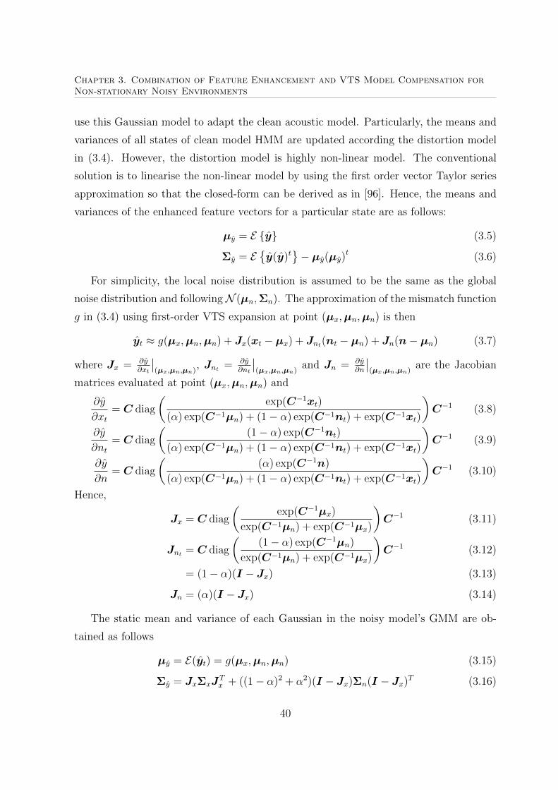
Chapter 3. Combination of Feature Enhancement and VTS Model Compensation forNon-stationary Noisy Environments
use this Gaussian model to adapt the clean acoustic model. Particularly, the means and
variances of all states of clean model HMM are updated according the distortion model
in (3.4). However, the distortion model is highly non-linear model. The conventional
solution is to linearise the non-linear model by using the first order vector Taylor series
approximation so that the closed-form can be derived as in [96]. Hence, the means and
variances of the enhanced feature vectors for a particular state are as follows:
µy = E {y} (3.5)
Σy = E{y(y)t
}− µy(µy)t (3.6)
For simplicity, the local noise distribution is assumed to be the same as the global
noise distribution and followingN (µn,Σn). The approximation of the mismatch function
g in (3.4) using first-order VTS expansion at point (µx,µn,µn) is then
yt ≈ g(µx,µn,µn) + Jx(xt − µx) + Jnt(nt − µn) + Jn(n− µn) (3.7)
where Jx = ∂y∂xt
∣∣(µx,µn,µn)
, Jnt = ∂y∂nt
∣∣(µx,µn,µn)
and Jn = ∂y∂n
∣∣(µx,µn,µn)
are the Jacobian
matrices evaluated at point (µx,µn,µn) and
∂y
∂xt= C diag
(exp(C−1xt)
(α) exp(C−1µn) + (1− α) exp(C−1nt) + exp(C−1xt)
)C−1 (3.8)
∂y
∂nt= C diag
((1− α) exp(C−1nt)
(α) exp(C−1µn) + (1− α) exp(C−1nt) + exp(C−1xt)
)C−1 (3.9)
∂y
∂n= C diag
((α) exp(C−1n)
(α) exp(C−1µn) + (1− α) exp(C−1nt) + exp(C−1xt)
)C−1 (3.10)
Hence,
Jx = C diag
(exp(C−1µx)
exp(C−1µn) + exp(C−1µx)
)C−1 (3.11)
Jnt = C diag
((1− α) exp(C−1µn)
exp(C−1µn) + exp(C−1µx)
)C−1 (3.12)
= (1− α)(I − Jx) (3.13)
Jn = (α)(I − Jx) (3.14)
The static mean and variance of each Gaussian in the noisy model’s GMM are ob-
tained as follows
µy = E(yt) = g(µx,µn,µn) (3.15)
Σy = JxΣxJTx + ((1− α)2 + α2)(I − Jx)Σn(I − Jx)T (3.16)
40
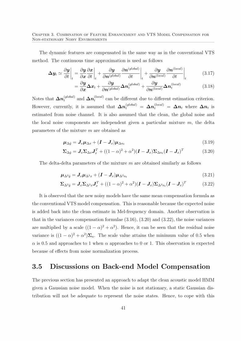
Chapter 3. Combination of Feature Enhancement and VTS Model Compensation forNon-stationary Noisy Environments
The dynamic features are compensated in the same way as in the conventional VTS
method. The continuous time approximation is used as follows
∆yt '∂y
∂t
∣∣∣∣t
=∂y
∂x
∂x
∂t
∣∣∣∣t
+∂y
∂n(global)
∂n(global)
∂t
∣∣∣∣t
+∂y
∂n(local)
∂n(local)
∂t
∣∣∣∣t
(3.17)
=∂y
∂x∆xt +
∂y
∂n(global)∆n
(global)t +
∂y
∂n(local)∆n
(local)t (3.18)
Notes that ∆n(global)t and ∆n
(local)t can be different due to different estimation criterion.
However, currently, it is assumed that ∆n(global)t = ∆n
(local)t = ∆nt where ∆nt is
estimated from noise channel. It is also assumed that the clean, the global noise and
the local noise components are independent given a particular mixture m, the delta
parameters of the mixture m are obtained as
µ∆y = Jxµ∆x + (I − Jx)µ∆nt (3.19)
Σ∆y = JxΣ∆xJTx + ((1− α)2 + α2)(I − Jx)Σ∆nt(I − Jx)T (3.20)
The delta-delta parameters of the mixture m are obtained similarly as follows
µ∆2y = Jxµ∆2x + (I − Jx)µ∆2nt(3.21)
Σ∆2y = JxΣ∆2xJTx + ((1− α)2 + α2)(I − Jx)Σ∆2nt
(I − Jx)T (3.22)
It is observed that the new noisy models have the same mean compensation formula as
the conventional VTS model compensation. This is reasonable because the expected noise
is added back into the clean estimate in Mel-frequency domain. Another observation is
that in the variances compensation formulae (3.16), (3.20) and (3.22), the noise variances
are multiplied by a scale ((1 − α)2 + α2). Hence, it can be seen that the residual noise
variance is ((1 − α)2 + α2)Σn. The scale value attains the minimum value of 0.5 when
α is 0.5 and approaches to 1 when α approaches to 0 or 1. This observation is expected
because of effects from noise normalization process.
3.5 Discussions on Back-end Model Compensation
The previous section has presented an approach to adapt the clean acoustic model HMM
given a Gaussian noise model. When the noise is not stationary, a static Gaussian dis-
tribution will not be adequate to represent the noise states. Hence, to cope with this
41
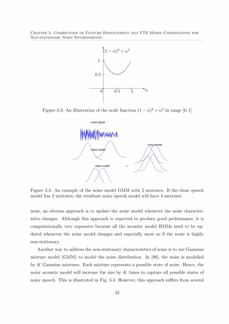
Chapter 3. Combination of Feature Enhancement and VTS Model Compensation forNon-stationary Noisy Environments
-
6
0 0.5 1
0.5
1
(1− α)2 + α2
α
Figure 3.3: An illustration of the scale function (1− α)2 + α2 in range [0, 1]
−2 −1 0 1 2 3 4 50
0.5
1
1.5
2
2.5
3
3.5
4
4.5
5
5.5
clean model
noise model
noise signal
→
noisy model
Figure 3.4: An example of the noise model GMM with 2 mixtures. If the clean speechmodel has 2 mixtures, the resultant noisy speech model will have 4 mixtures
issue, an obvious approach is to update the noise model whenever the noise character-
istics changes. Although this approach is expected to produce good performance, it is
computationally very expensive because all the acoustic model HMMs need to be up-
dated whenever the noise model changes and especially more so if the noise is highly
non-stationary.
Another way to address the non-stationary characteristics of noise is to use Gaussian
mixture model (GMM) to model the noise distribution. In [90], the noise is modelled
by K Gaussian mixtures. Each mixture represents a possible state of noise. Hence, the
noisy acoustic model will increase the size by K times to capture all possible states of
noisy speech. This is illustrated in Fig. 3.4. However, this approach suffers from several
42
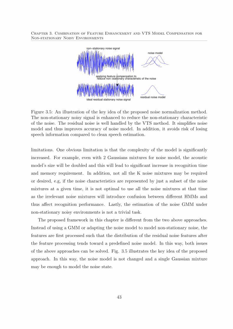
Chapter 3. Combination of Feature Enhancement and VTS Model Compensation forNon-stationary Noisy Environments
−1 0 1 2 3 4 5 6 7 8 9 10
−6
−4
−2
0
2
4
6 non−stationary noise signal
ideal residual stationary noise signal
applying feature compensation toreduce non−stationary characteristic of the noise
noise model
residual noise model
Figure 3.5: An illustration of the key idea of the proposed noise normalization method.The non-stationary noisy signal is enhanced to reduce the non-stationary characteristicof the noise. The residual noise is well handled by the VTS method. It simplifies noisemodel and thus improves accuracy of noise model. In addition, it avoids risk of losingspeech information compared to clean speech estimation.
limitations. One obvious limitation is that the complexity of the model is significantly
increased. For example, even with 2 Gaussians mixtures for noise model, the acoustic
model’s size will be doubled and this will lead to significant increase in recognition time
and memory requirement. In addition, not all the K noise mixtures may be required
or desired, e.g, if the noise characteristics are represented by just a subset of the noise
mixtures at a given time, it is not optimal to use all the noise mixtures at that time
as the irrelevant noise mixtures will introduce confusion between different HMMs and
thus affect recognition performance. Lastly, the estimation of the noise GMM under
non-stationary noisy environments is not a trivial task.
The proposed framework in this chapter is different from the two above approaches.
Instead of using a GMM or adapting the noise model to model non-stationary noise, the
features are first processed such that the distribution of the residual noise features after
the feature processing tends toward a predefined noise model. In this way, both issues
of the above approaches can be solved. Fig. 3.5 illustrates the key idea of the proposed
approach. In this way, the noise model is not changed and a single Gaussian mixture
may be enough to model the noise state.
43
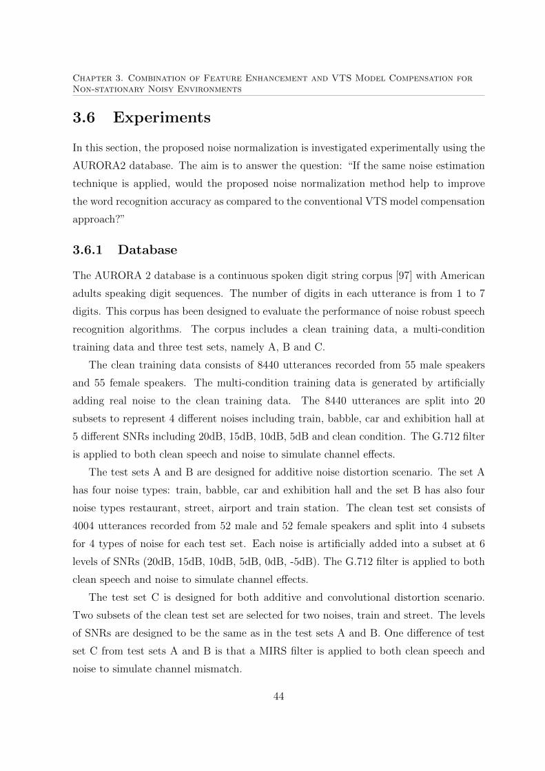
Chapter 3. Combination of Feature Enhancement and VTS Model Compensation forNon-stationary Noisy Environments
3.6 Experiments
In this section, the proposed noise normalization is investigated experimentally using the
AURORA2 database. The aim is to answer the question: “If the same noise estimation
technique is applied, would the proposed noise normalization method help to improve
the word recognition accuracy as compared to the conventional VTS model compensation
approach?”
3.6.1 Database
The AURORA 2 database is a continuous spoken digit string corpus [97] with American
adults speaking digit sequences. The number of digits in each utterance is from 1 to 7
digits. This corpus has been designed to evaluate the performance of noise robust speech
recognition algorithms. The corpus includes a clean training data, a multi-condition
training data and three test sets, namely A, B and C.
The clean training data consists of 8440 utterances recorded from 55 male speakers
and 55 female speakers. The multi-condition training data is generated by artificially
adding real noise to the clean training data. The 8440 utterances are split into 20
subsets to represent 4 different noises including train, babble, car and exhibition hall at
5 different SNRs including 20dB, 15dB, 10dB, 5dB and clean condition. The G.712 filter
is applied to both clean speech and noise to simulate channel effects.
The test sets A and B are designed for additive noise distortion scenario. The set A
has four noise types: train, babble, car and exhibition hall and the set B has also four
noise types restaurant, street, airport and train station. The clean test set consists of
4004 utterances recorded from 52 male and 52 female speakers and split into 4 subsets
for 4 types of noise for each test set. Each noise is artificially added into a subset at 6
levels of SNRs (20dB, 15dB, 10dB, 5dB, 0dB, -5dB). The G.712 filter is applied to both
clean speech and noise to simulate channel effects.
The test set C is designed for both additive and convolutional distortion scenario.
Two subsets of the clean test set are selected for two noises, train and street. The levels
of SNRs are designed to be the same as in the test sets A and B. One difference of test
set C from test sets A and B is that a MIRS filter is applied to both clean speech and
noise to simulate channel mismatch.
44
Chapter 3. Combination of Feature Enhancement and VTS Model Compensation forNon-stationary Noisy Environments
10 20 30 40 50 60 70 80 90 100
−1.5
−1
−0.5
0
0.5
1
1.5
2
2.5
3
time
log
(mel)
TESTA/N1SNR−5/FAK
1B.08; the 4th bin
smoothed version,wsize=5
true noise
Figure 3.6: An example of the smoothed version of the ideal noise in log-Mel domain.The fourth bin is plotted.
Test sets A and B are selected to evaluate the proposed method as we will first
examine only the additive noise problem. The ground truth noise can be obtained by
subtracting the clean signal from the noisy signal. To proceed in evaluating the proposed
work under a fixed noise estimation framework, we first employ a smoothed version of
the true noise features in the cepstral domain to examine the system’s performance. In
another words, we use the smoothed version of the true noise to simulate the estimation
of the noise. We will use actual estimate of the noise in future works. An example of
the smoothed version of the true noise features is illustrated in Fig. 3.6. The use of the
smooth noise is to limit the analysis so that error caused by the noise estimation can be
controlled.
3.6.2 System Configurations
The standard ASR system as in [97] is used for the baseline system. In the front-end
configurations, the standard 39-MFCC features are used which consist of the first 13
cepstral coefficients, 13 delta features and 13 delta-delta features. The HMM acoustic
model as in [97] is used. Particularly, each digit HMM consists of 16 emitting states and
45
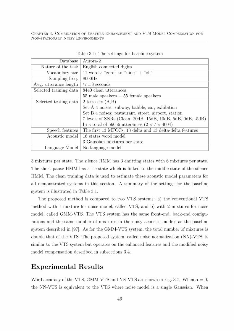
Chapter 3. Combination of Feature Enhancement and VTS Model Compensation forNon-stationary Noisy Environments
Table 3.1: The settings for baseline system
Database Aurora-2Nature of the task English connected digits
Vocabulary size 11 words: “zero” to “nine” + “oh”Sampling freq. 8000Hz
Avg. utterance length ≈ 1.8 secondsSelected training data 8440 clean utterances
55 male speakers + 55 female speakersSelected testing data 2 test sets (A,B)
Set A 4 noises: subway, babble, car, exhibitionSet B 4 noises: restaurant, street, airport, station7 levels of SNRs (Clean, 20dB, 15dB, 10dB, 5dB, 0dB, -5dB)In a total of 56056 utterances (2× 7× 4004)
Speech features The first 13 MFCCs, 13 delta and 13 delta-delta featuresAcoustic model 16 states word model
3 Gaussian mixtures per stateLanguage Model No language model
3 mixtures per state. The silence HMM has 3 emitting states with 6 mixtures per state.
The short pause HMM has a tie-state which is linked to the middle state of the silence
HMM. The clean training data is used to estimate these acoustic model parameters for
all demonstrated systems in this section. A summary of the settings for the baseline
system is illustrated in Table 3.1.
The proposed method is compared to two VTS systems: a) the conventional VTS
method with 1 mixture for noise model, called VTS, and b) with 2 mixtures for noise
model, called GMM-VTS. The VTS system has the same front-end, back-end configu-
rations and the same number of mixtures in the noisy acoustic models as the baseline
system described in [97]. As for the GMM-VTS system, the total number of mixtures is
double that of the VTS. The proposed system, called noise normalization (NN)-VTS, is
similar to the VTS system but operates on the enhanced features and the modified noisy
model compensation described in subsections 3.4.
Experimental Results
Word accuracy of the VTS, GMM-VTS and NN-VTS are shown in Fig. 3.7. When α = 0,
the NN-VTS is equivalent to the VTS where noise model is a single Gaussian. When
46
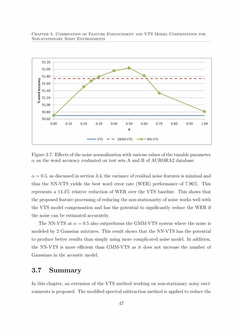
Chapter 3. Combination of Feature Enhancement and VTS Model Compensation forNon-stationary Noisy Environments
Figure 3.7: Effects of the noise normalization with various values of the tunable parameterα on the word accuracy evaluated on test sets A and B of AURORA2 database
α = 0.5, as discussed in section 3.4, the variance of residual noise features is minimal and
thus the NN-VTS yields the best word error rate (WER) performance of 7.96%. This
represents a 14.4% relative reduction of WER over the VTS baseline. This shows that
the proposed feature processing of reducing the non-stationarity of noise works well with
the VTS model compensation and has the potential to significantly reduce the WER if
the noise can be estimated accurately.
The NN-VTS at α = 0.5 also outperforms the GMM-VTS system where the noise is
modeled by 2 Gaussian mixtures. This result shows that the NN-VTS has the potential
to produce better results than simply using more complicated noise model. In addition,
the NN-VTS is more efficient than GMM-VTS as it does not increase the number of
Gaussians in the acoustic model.
3.7 Summary
In this chapter, an extension of the VTS method working on non-stationary noisy envi-
ronments is proposed. The modified spectral subtraction method is applied to reduce the
47
Chapter 3. Combination of Feature Enhancement and VTS Model Compensation forNon-stationary Noisy Environments
non-stationary characteristic of the noise. Hence, the residual noise is more stationary
than the original noise and better modeled in the VTS model compensation. A smoothed
version of the true noise is used to investigate the potential of the proposed method. The
simulation results on Aurora-2 task show that significant performance improvement is
possible over the conventional VTS model compensation.
A limitation of the proposed method is that its performance will be dependent on how
accurately can the non-stationary noise be estimated. Estimating non-stationary noise
remains a hard task due to the unknown and unpredictable nature of non-stationary
noise. It is even harder than estimating directly clean speech features because clean
speech is predictable. Therefore, instead of trying to estimate non-stationary noise, in
the next proposed method, clean speech feature estimation is considered and presented
in next chapter.
48
Chapter 4
A Particle Filter CompensationApproach to Robust LVCSR
Recently, Mushtaq et. al. [35] proposed a novel enhancement approach for ASR by
estimating clean speech features in noisy environment. The approach generates clean
speech features by utilizing estimated state sequence of hidden Markov models (HMMs)
of clean speech in the particle filter framework. However, under noisy conditions, the
task to estimate an accurate HMM state sequence that describes the underlying clean
speech features is challenging as the speech is distorted in noisy environments. This work
proposes to extend on [35] by applying two acoustic models, clean and noisy models, for
its operations. Specifically, given the observed noisy features, the noisy model is used by
the decoder to estimate the speech’s phone state sequence, and from this estimated state
sequence, the corresponding clean state sequence is predicted. This clean state sequence
and the clean model are then exploited by the particle filter to perform enhancement. The
performance of this approach depends significantly on the ability to obtain an accurately
aligned state and mixture sequence of hidden Markov models (HMMs) that describe
the underlying clean speech features under noisy environment. This chapter presents a
solution for the alignment issue and has been reported in [34].
4.1 Introduction
One common estimation problem is to determine the true value of a system given only
some noisy observations of that system. Examples include the tracking location of an
49
Chapter 4. A Particle Filter Compensation Approach to Robust LVCSR
aircraft from radar, estimating communications signals from noisy measurements. One
method used to solve this problem is by particle filter [98]. Particle filter belongs to
the class of Monte Carlo method and is versatile. It can handle a broad category of
dynamical systems not constrained by linearity and Gaussianity requirements of Kalman
Filter [99] and extended Kalman Filter [100].
In the speech enhancement domain, particle filters were initially used to track noise
information in noisy signals to obtain compensated clean features [101–103]. Here, noise
is treated as a state variable while speech is considered as the signal corrupting the obser-
vation noise. In another approach, particle filter compensation (PFC) [35,104] algorithms
compensated noisy speech features by directly tracking the clean speech features in the
spectral domain, i.e., the speech feature in spectral domain is treated as a state variable
while noise is considered as the signal corrupting the speech feature.
To apply particle filters, a state transition model that adequately captures the dy-
namic properties of the speech signal is required. Due to the nature of speech, it is
difficult to find such a model. The PFC approach has somewhat overcome the prob-
lem by introducing information from HMMs trained with clean speech to propagate the
particles. Nevertheless, under noisy condition, the speech is distorted and it remains
challenging to accurately select the proper state of clean feature for the PFC algorithm.
The difficulty is increased for large vocabulary systems because the number of triphone
HMMs used can be very large, e.g. exceeding 10, 000 states.
To overcome this problem, we extended the PFC approach by using two HMM models
such that one noisy model is used to estimate the state sequence and one clean model
is used to generate clean speech features. To closely link the states of these two models,
they are jointly trained using single pass retraining (SPR) technique [105] from parallel
data (i.e. one clean channel and one noisy channel). In addition, to reduce the effects of
choosing wrong states, we group similar states into one cluster, called physical state, by
using the furthest neighbour hierarchical cluster algorithm [105]. Hence, in our proposed
PFC system, the noisy model helps to improve the accuracy of the state estimation, and
clustering reduces the erroneous choice of HMM states.
The proposed PFC system is tested on the Aurora-4 large vocabulary continuous
speech recognition task. Our results in [34] shows that a large error reduction of 28.46%
50
Chapter 4. A Particle Filter Compensation Approach to Robust LVCSR
is achieved with 120 clusters (physical states), if the side information (i.e. the state se-
quence) is accurately known. Similarly good performance is maintained (error reduction
of 20.66% and 19.97% respectively) even when fewer number of states such as 10 phys-
ical states and 5 physical states are used. However, in actual scenarios, the best error
reduction achieved is only 5.3% and that is with 3 physical states. Details of the works
are presented in the following sections.
4.2 Tracking Sequence of Clean Speech Features us-
ing PFC
4.2.1 Using HMM States to Generate Samples
HMMs differ in nature from the standard particle filter (PF) tracking algorithms, and
by themselves have limited capability to track a continuously varying signal. Although
both HMMs and PF have states, these states are different in nature. The state of a
PF is a real quantity, while the states of an HMM should only be used as a modeling
strategy. The observation distribution of an HMM, however, is a real quantity, and can
be a valid source for sample generation. Consequently, there is a possibility to utilize
the observation distribution to generate samples in the PF framework and from them,
estimate the clean features. This idea is illustrated in the lower part of Fig. 4.1.
In Fig. 4.1, the solid line in the upper part represents the sequence of the observed
speech feature vectors and the dash line in the lower part represents the estimated se-
quence of the clean speech features. The circle symbols S1, S2 and S3 are the HMM
states whose observation distribution is used to generate the samples of the state. In-
stead of obtaining the samples from the state space model as is done in a conventional PF
algorithm, the samples are generated from the observation model of the corresponding
state of a clean HMM model. In this work, the clean state is deduced from noisy state
of speech feature. In the figure, the diameter of the sample indicates its weight which
approximates the posterior density (i.e. the higher the density, the greater the weight).
The weights can be estimated by using a distortion model of noisy speech. In this work,
we use a simple distortion model which is presented in next subsection.
51
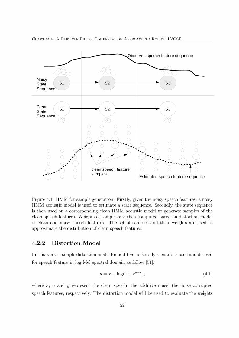
Chapter 4. A Particle Filter Compensation Approach to Robust LVCSR
S1 S2 S3
S1 S2 S3
Observed speech feature sequence
Estimated speech feature sequence
clean speech feature samples
NoisyStateSequence
CleanStateSequence
Figure 4.1: HMM for sample generation. Firstly, given the noisy speech features, a noisyHMM acoustic model is used to estimate a state sequence. Secondly, the state sequenceis then used on a corresponding clean HMM acoustic model to generate samples of theclean speech features. Weights of samples are then computed based on distortion modelof clean and noisy speech features. The set of samples and their weights are used toapproximate the distribution of clean speech features.
4.2.2 Distortion Model
In this work, a simple distortion model for additive noise only scenario is used and derived
for speech feature in log Mel spectral domain as follow [51]:
y = x+ log(1 + en−x), (4.1)
where x, n and y represent the clean speech, the additive noise, the noise corrupted
speech features, respectively. The distortion model will be used to evaluate the weights
52
Chapter 4. A Particle Filter Compensation Approach to Robust LVCSR
of clean feature samples in PFC algorithm.
4.2.3 A Brief Discussion of using PFC
In the recognition phase, there are 3 steps. In step 1, we decode the input features to
generate a state sequence of speech features. In step 2, the state sequence is used to
enhance the speech features by using the PFC method. Finally, in step 3, we decode the
enhanced features to generate an output hypothesis. The speech enhancement in step 2
is summarised in this section.
In step 2, given a state sequence of speech features, the task is to estimate clean speech
features. We first estimate the noise model from non-speech frames which belong to the
given non-speech states. For simplicity, we assume the noise is a Gaussian N (µn, σn).
Then at each time t, speech tracking using PFC as used in our work is summarized as
follows [34,35,104]:
(i) The posterior density of the clean speech features at time t is represented by a finite
number of support points,
p(xt|y0: t) =Ns∑i=1
witδ(xt − xit) (4.2)
where xit for i = 1, ..., Ns are the support points of the PF and δ() denotes the Dirac
delta function.
(ii) The weights of the support points, wit, are computed based on the concept of
importance sampling 1 as follow [106]:
wit = wit−1
p(yt|xit)p(xit|xit−1)
q(xit|xit−1, yt)(4.3)
where q(xit|xit−1, yt) is the importance sampling density. The set of supported points
with the weights will approximate the posterior density of speech features.
1Importance sampling is a trick that samples from the available distribution q and re-weight samplesto fix it into the required distribution p. In this work, we use the simplest form where p = q. It is knownas the sampling importance resampling (SIR) filter.
53
Chapter 4. A Particle Filter Compensation Approach to Robust LVCSR
(iii) Using the distortion model of speech features in log Mel spectral domain with no
channel effects (4.1), p(yt|xit) can be approximated as
p(yt|xit) = F ′(uit) = p(uit)eyt−x
it
eyt−xit − 1
(4.4)
where F (.) is the Gaussian cumulative function with mean µn and variance σ2n.
Note that p(u) = N (µn, σn) is the noise model and
uit = log(eyt−xit − 1) + xit (4.5)
(iv) The density q(xit|xit−1, yt) is used to generate speech samples. The distribution is
obtained by choosing a state (or a cluster) from HMMs which is given in step 2.
(v) Finally, the compensated features are estimated as [35]:
xt =Ns∑i=1
witxit (4.6)
4.3 PFC for LVCSR
In LVCSR systems, subword acoustic models on MFCC features are a popular choice
and triphone representation achieves the best recognition performance. There are two
problems when applying PFC for LVCSR. The first problem is the mismatch of speech
features used by the decoder and PFC. While the decoder chooses the MFCC features
to achieve the best performance, PFC needs to work on FBANK features due to the
current distortion model of noisy speech. The second problem is to estimate a state of
clean speech features for a particular frame so that the samples can be generated from its
distribution that precisely represents the clean speech features for that frame. In noisy
condition, using clean acoustic models for decoding perform poorly on noisy features.
To solve the above two problems, we propose to build a link from a state of noisy
speech feature to a distribution of clean speech features which can be used to generate
samples of clean speech features as follows. A noisy triphone HMM acoustic model is
firstly used by the decoder to generate a noisy triphone state sequence. The noisy triphone
state sequence is then used to deduce a clean triphone state sequence. Ignoring the
54
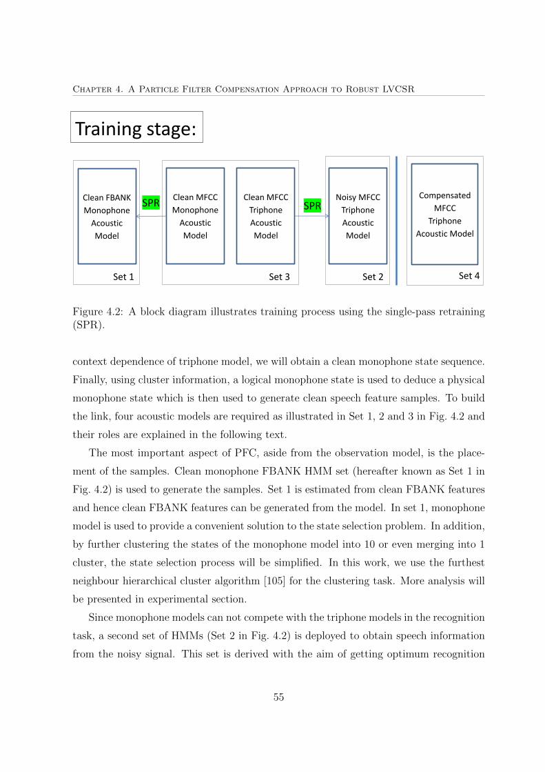
Chapter 4. A Particle Filter Compensation Approach to Robust LVCSR
Clean FBANK
Monophone
Acoustic
Model
Clean MFCC
Monophone
Acoustic
Model
Clean MFCC
Triphone
Acoustic
Model
Noisy MFCC
Triphone
Acoustic
Model
Training stage:
SPR SPR
Set 1 Set 2 Set 3
Compensated
MFCC
Triphone
Acoustic Model
Set 4
Figure 4.2: A block diagram illustrates training process using the single-pass retraining(SPR).
context dependence of triphone model, we will obtain a clean monophone state sequence.
Finally, using cluster information, a logical monophone state is used to deduce a physical
monophone state which is then used to generate clean speech feature samples. To build
the link, four acoustic models are required as illustrated in Set 1, 2 and 3 in Fig. 4.2 and
their roles are explained in the following text.
The most important aspect of PFC, aside from the observation model, is the place-
ment of the samples. Clean monophone FBANK HMM set (hereafter known as Set 1 in
Fig. 4.2) is used to generate the samples. Set 1 is estimated from clean FBANK features
and hence clean FBANK features can be generated from the model. In set 1, monophone
model is used to provide a convenient solution to the state selection problem. In addition,
by further clustering the states of the monophone model into 10 or even merging into 1
cluster, the state selection process will be simplified. In this work, we use the furthest
neighbour hierarchical cluster algorithm [105] for the clustering task. More analysis will
be presented in experimental section.
Since monophone models can not compete with the triphone models in the recognition
task, a second set of HMMs (Set 2 in Fig. 4.2) is deployed to obtain speech information
from the noisy signal. This set is derived with the aim of getting optimum recognition
55
Chapter 4. A Particle Filter Compensation Approach to Robust LVCSR
performance. Hence, the HMMs in set 2 are triphone models built using multi-condition
MFCC features.
As the HMMs in Set 2 are used to select the appropriate state from HMMs in Set
1, a good alignment between the two sets is essential to obtain good performance with
PFC algorithm. The two sets, however, use different features, structures (one is made
up of monophone while the other of triphone models) and data (one uses clean FBANK
features and the other uses noisy MFCC features). Consequently, the two sets can be
severely misaligned. To overcome this problem, the clean MFCC HMMs (Set 3) are
used as the source and both Set 1 and Set 2 are derived from it. The technique for this
alignment procedure is explained in Fig. 4.2.
We train Set 1 HMMs in 2 steps. Step 1 computes forward and backward probabil-
ities using clean MFCC monophone HMMs on clean MFCC features. Step 2 estimates
parameters of FBANK monophone HMMs using the statistics information from Step 1,
together with clean FBANK features. This is known as single-pass retraining [93].
In this way, the state/phone alignment (i.e., the posterior component probabilities)
used to estimate parameters of monophone FBANK HMMs is the same as one generated
by using the monophone MFCC HMMs. Therefore, same component label of two states
in two different feature domain will model the same sound but in two different feature
domain.
Training HMMs in Set 2 is similar. Step 1 compute forward and backward probabili-
ties using triphone HMMs on clean MFCC features. Step 2 estimates HMM parameters
using the statistics from Step 1 along with noisy MFCC features.
Since all HMM parameters in Sets 1 and 2 are estimated based on state alignment
computed from clean MFCC HMMs, a state mapping between the two sets can be ob-
tained by just using the same component labels.
In the recognition phase, as the final recognition of the compensated data can be
isolated from the compensation process, we train another HMM acoustic model as illus-
trated in Set 4 from multi-condition training data that has been compensated like we
would process the test data in actual scenario. Since there are no constrains on these
models, their complexity can be increased to the optimum level needed to obtain the best
possible recognition performance.
56
Chapter 4. A Particle Filter Compensation Approach to Robust LVCSR
4.4 Aurora-4 Experiments
In the following, PFC experiments are conducted on the Aurora-4 task. An oracle ex-
periment with high accuracy of state sequence estimation is firstly conducted to focus on
optimizing particle sampling and evaluate the upper bound of the method. An actual
experiment is then conducted to evaluate the performance of the system.
4.4.1 General Configurations
The hidden Markov model toolkit (HTK) [105] was used to extract speech features and
train acoustic models. Log mel filter bank (FBANK) coefficients (23 coefficients) were
extracted from 16KHz sampled speech signals and enhanced by PFC method. Mel-
frequency cepstral coefficients (13 coefficients) and their first and second differential fea-
tures are then extracted from compensated FBANK and used as speech features for
speech recognizer. Ceptral mean normalization was also applied to reduce the channel
mismatch. A bigram language model was used with language model scale factor set to
15.
The four acoustic models were trained as described earlier. In this study, HMMs in
Set 1 have 120 states with 3 Gaussian mixtures per state. The triphone HMMs in Set 2,
3 and 4 were the same and have 1594 tied-states with 16 Gaussian mixtures per state.
In the testing phase, we are interested in additive background noises. Six noisy test
sets (car, babble, restaurant, street, airport and train noises) without channel mismatch
were used to evaluate the PFC performance. The noise statistics are estimated from
silence frames of each utterance.
As PFC works in the FBANK domain, the compensated FBANK features are then
transformed to MFCC domain by DCT transformation. For dynamic features (delta and
delta-delta features), we have two options: re-compute the dynamic features from the
compensated MFCC features or just use the original noisy dynamic features. We will
discuss about the two options in more details in the next sections.
4.4.2 Experiments with Oracle Cluster ID
To estimate the potential of PFC, we first build an oracle experiment with high accuracy
of cluster selection. In this experiment, we utilize the stereo data in Aurora-4 to generate
57
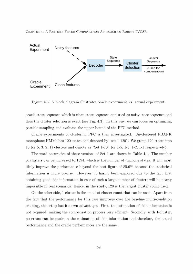
Chapter 4. A Particle Filter Compensation Approach to Robust LVCSR
Noisy features
Clean features
Decoder
OracleExperiment
ActualExperiment
ClusterSelection
StateSequence
ClusterSequence
(Used for compensation)
Figure 4.3: A block diagram illustrates oracle experiment vs. actual experiment.
oracle state sequence which is clean state sequence and used as noisy state sequence and
thus the cluster selection is exact (see Fig. 4.3). In this way, we can focus on optimizing
particle sampling and evaluate the upper bound of the PFC method.
Oracle experiments of clustering PFC is then investigated. Un-clustered FBANK
monophone HMMs has 120 states and denoted by “set 1-120”. We group 120 states into
10 (or 5, 3, 2, 1) clusters and denote as “Set 1-10” (or 1-5, 1-3, 1-2, 1-1 respectively).
The word accuracies of these versions of Set 1 are shown in Table 4.1. The number
of clusters can be increased to 1594, which is the number of triphone states. It will most
likely improve the performance beyond the best figure of 85.6% because the statistical
information is more precise. However, it hasn’t been explored due to the fact that
obtaining good side information in case of such a large number of clusters will be nearly
impossible in real scenarios. Hence, in the study, 120 is the largest cluster count used.
On the other side, 1-cluster is the smallest cluster count that can be used. Apart from
the fact that the performance for this case improves over the baseline multi-condition
training, the setup has it’s own advantages. First, the estimation of side information is
not required, making the compensation process very efficient. Secondly, with 1-cluster,
no errors can be made in the estimation of side information and therefore, the actual
performance and the oracle performances are the same.
58
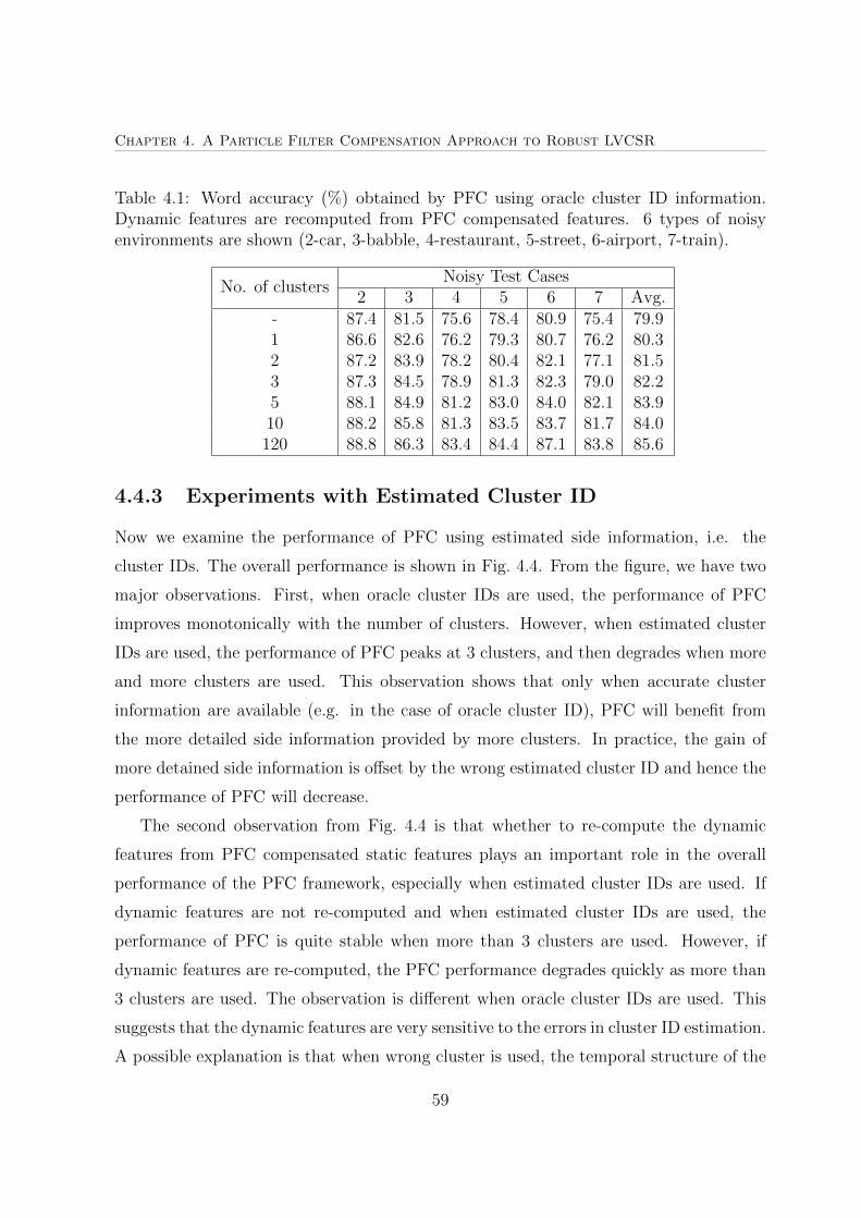
Chapter 4. A Particle Filter Compensation Approach to Robust LVCSR
Table 4.1: Word accuracy (%) obtained by PFC using oracle cluster ID information.Dynamic features are recomputed from PFC compensated features. 6 types of noisyenvironments are shown (2-car, 3-babble, 4-restaurant, 5-street, 6-airport, 7-train).
No. of clustersNoisy Test Cases
2 3 4 5 6 7 Avg.- 87.4 81.5 75.6 78.4 80.9 75.4 79.91 86.6 82.6 76.2 79.3 80.7 76.2 80.32 87.2 83.9 78.2 80.4 82.1 77.1 81.53 87.3 84.5 78.9 81.3 82.3 79.0 82.25 88.1 84.9 81.2 83.0 84.0 82.1 83.910 88.2 85.8 81.3 83.5 83.7 81.7 84.0120 88.8 86.3 83.4 84.4 87.1 83.8 85.6
4.4.3 Experiments with Estimated Cluster ID
Now we examine the performance of PFC using estimated side information, i.e. the
cluster IDs. The overall performance is shown in Fig. 4.4. From the figure, we have two
major observations. First, when oracle cluster IDs are used, the performance of PFC
improves monotonically with the number of clusters. However, when estimated cluster
IDs are used, the performance of PFC peaks at 3 clusters, and then degrades when more
and more clusters are used. This observation shows that only when accurate cluster
information are available (e.g. in the case of oracle cluster ID), PFC will benefit from
the more detailed side information provided by more clusters. In practice, the gain of
more detained side information is offset by the wrong estimated cluster ID and hence the
performance of PFC will decrease.
The second observation from Fig. 4.4 is that whether to re-compute the dynamic
features from PFC compensated static features plays an important role in the overall
performance of the PFC framework, especially when estimated cluster IDs are used. If
dynamic features are not re-computed and when estimated cluster IDs are used, the
performance of PFC is quite stable when more than 3 clusters are used. However, if
dynamic features are re-computed, the PFC performance degrades quickly as more than
3 clusters are used. The observation is different when oracle cluster IDs are used. This
suggests that the dynamic features are very sensitive to the errors in cluster ID estimation.
A possible explanation is that when wrong cluster is used, the temporal structure of the
59
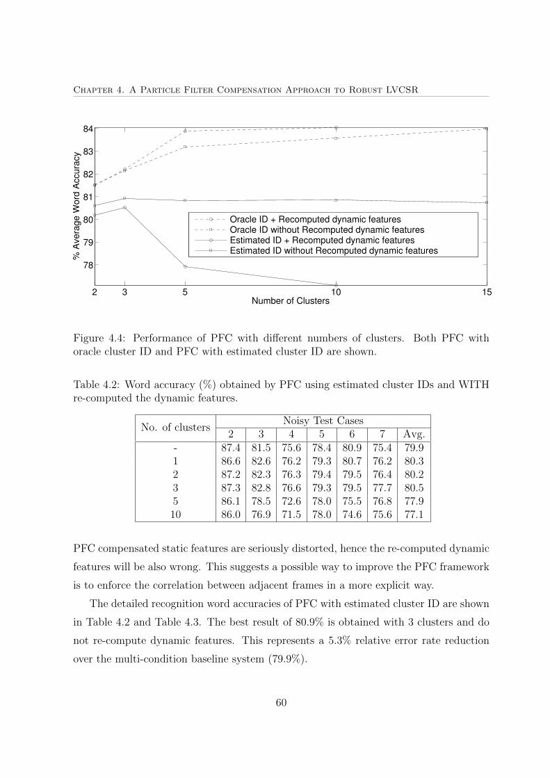
Chapter 4. A Particle Filter Compensation Approach to Robust LVCSR
2 3 5 10 15
78
79
80
81
82
83
84
Number of Clusters
% A
vera
ge W
ord
Accura
cy
Oracle ID + Recomputed dynamic featuresOracle ID without Recomputed dynamic featuresEstimated ID + Recomputed dynamic featuresEstimated ID without Recomputed dynamic features
Figure 4.4: Performance of PFC with different numbers of clusters. Both PFC withoracle cluster ID and PFC with estimated cluster ID are shown.
Table 4.2: Word accuracy (%) obtained by PFC using estimated cluster IDs and WITHre-computed the dynamic features.
No. of clustersNoisy Test Cases
2 3 4 5 6 7 Avg.- 87.4 81.5 75.6 78.4 80.9 75.4 79.91 86.6 82.6 76.2 79.3 80.7 76.2 80.32 87.2 82.3 76.3 79.4 79.5 76.4 80.23 87.3 82.8 76.6 79.3 79.5 77.7 80.55 86.1 78.5 72.6 78.0 75.5 76.8 77.910 86.0 76.9 71.5 78.0 74.6 75.6 77.1
PFC compensated static features are seriously distorted, hence the re-computed dynamic
features will be also wrong. This suggests a possible way to improve the PFC framework
is to enforce the correlation between adjacent frames in a more explicit way.
The detailed recognition word accuracies of PFC with estimated cluster ID are shown
in Table 4.2 and Table 4.3. The best result of 80.9% is obtained with 3 clusters and do
not re-compute dynamic features. This represents a 5.3% relative error rate reduction
over the multi-condition baseline system (79.9%).
60
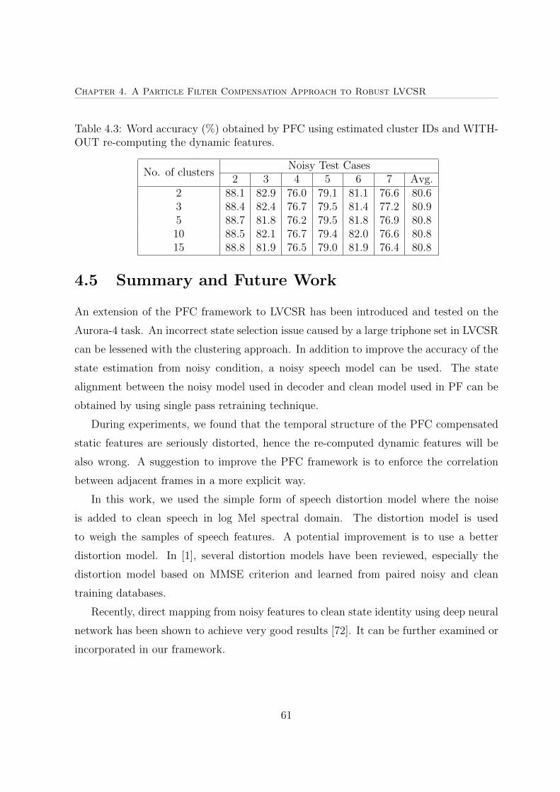
Chapter 4. A Particle Filter Compensation Approach to Robust LVCSR
Table 4.3: Word accuracy (%) obtained by PFC using estimated cluster IDs and WITH-OUT re-computing the dynamic features.
No. of clustersNoisy Test Cases
2 3 4 5 6 7 Avg.2 88.1 82.9 76.0 79.1 81.1 76.6 80.63 88.4 82.4 76.7 79.5 81.4 77.2 80.95 88.7 81.8 76.2 79.5 81.8 76.9 80.810 88.5 82.1 76.7 79.4 82.0 76.6 80.815 88.8 81.9 76.5 79.0 81.9 76.4 80.8
4.5 Summary and Future Work
An extension of the PFC framework to LVCSR has been introduced and tested on the
Aurora-4 task. An incorrect state selection issue caused by a large triphone set in LVCSR
can be lessened with the clustering approach. In addition to improve the accuracy of the
state estimation from noisy condition, a noisy speech model can be used. The state
alignment between the noisy model used in decoder and clean model used in PF can be
obtained by using single pass retraining technique.
During experiments, we found that the temporal structure of the PFC compensated
static features are seriously distorted, hence the re-computed dynamic features will be
also wrong. A suggestion to improve the PFC framework is to enforce the correlation
between adjacent frames in a more explicit way.
In this work, we used the simple form of speech distortion model where the noise
is added to clean speech in log Mel spectral domain. The distortion model is used
to weigh the samples of speech features. A potential improvement is to use a better
distortion model. In [1], several distortion models have been reviewed, especially the
distortion model based on MMSE criterion and learned from paired noisy and clean
training databases.
Recently, direct mapping from noisy features to clean state identity using deep neural
network has been shown to achieve very good results [72]. It can be further examined or
incorporated in our framework.
61
Chapter 5
Feature Adaptation UsingSpectro-Temporal Information
In the two previous proposed methods, the feature enhancement approach is based on a
physical distortion model of speech signal in noisy environments. However the physical
distortion is usually very complicated and it is hard to model it well. Particularly, the
two previous proposed methods had only assumed that the distortion is additive noise.
In this chapter, we disregard the physical distortion model and examine a general linear
transform approach to directly transform run-time speech features to expected clean
features.
Motivated by the finding that human speech comprehension relies on the integrity
of both the spectral content and temporal envelope of speech signal, a spectro-temporal
transform, which is a generalized linear feature transform, is proposed. The objective
of the transform is to modify the run-time speech features such that it minimizes the
mismatch between run-time and training data. In the scope of this work, spectral content
represents short term speech information within a frame of a few tens of milliseconds,
while temporal envelop captures the evolution of speech statistics over several consecutive
frames. A Kullback Leibler divergence based cost function is applied to estimate the
transform parameters. Experiments are conducted on the REVERB Challenge 2014 task,
where clean and multi-condition trained acoustic models are tested with real reverberant
and noisy speech. We found that temporal information is important for reverberant
speech recognition and the simultaneous use of spectral and temporal information for
feature adaptation is effective. All experiments consistently report significant word error
rate reductions and the work was published in [36].
62
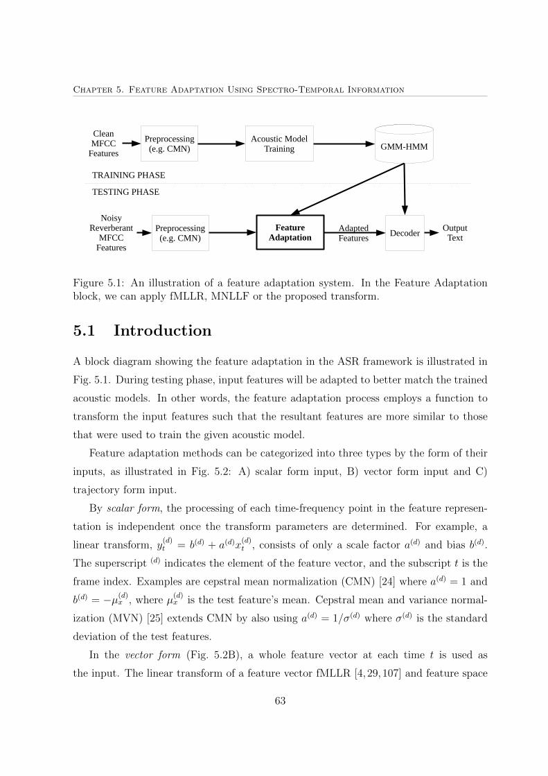
Chapter 5. Feature Adaptation Using Spectro-Temporal Information
Preprocessing(e.g. CMN)
Preprocessing(e.g. CMN)
Acoustic ModelTraining
CleanMFCC
Features
NoisyReverberant
MFCCFeatures
GMM-HMM
FeatureAdaptation Decoder
OutputText
TRAINING PHASE
TESTING PHASE
AdaptedFeatures
Figure 5.1: An illustration of a feature adaptation system. In the Feature Adaptationblock, we can apply fMLLR, MNLLF or the proposed transform.
5.1 Introduction
A block diagram showing the feature adaptation in the ASR framework is illustrated in
Fig. 5.1. During testing phase, input features will be adapted to better match the trained
acoustic models. In other words, the feature adaptation process employs a function to
transform the input features such that the resultant features are more similar to those
that were used to train the given acoustic model.
Feature adaptation methods can be categorized into three types by the form of their
inputs, as illustrated in Fig. 5.2: A) scalar form input, B) vector form input and C)
trajectory form input.
By scalar form, the processing of each time-frequency point in the feature represen-
tation is independent once the transform parameters are determined. For example, a
linear transform, y(d)t = b(d) + a(d)x
(d)t , consists of only a scale factor a(d) and bias b(d).
The superscript (d) indicates the element of the feature vector, and the subscript t is the
frame index. Examples are cepstral mean normalization (CMN) [24] where a(d) = 1 and
b(d) = −µ(d)x , where µ
(d)x is the test feature’s mean. Cepstral mean and variance normal-
ization (MVN) [25] extends CMN by also using a(d) = 1/σ(d) where σ(d) is the standard
deviation of the test features.
In the vector form (Fig. 5.2B), a whole feature vector at each time t is used as
the input. The linear transform of a feature vector fMLLR [4,29,107] and feature space
63
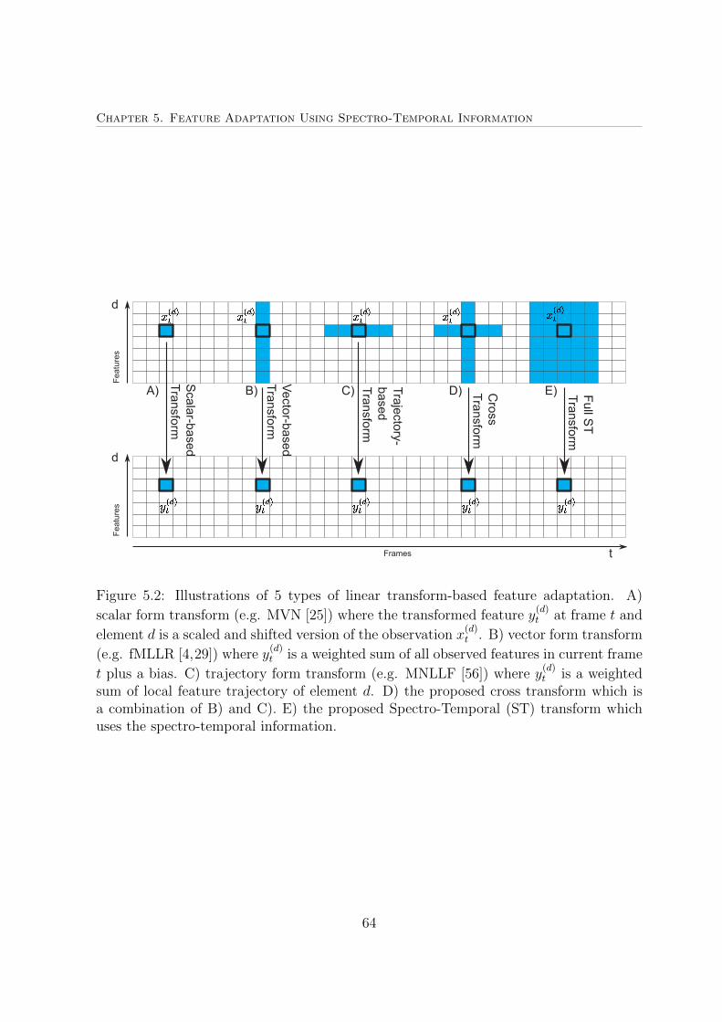
Chapter 5. Feature Adaptation Using Spectro-Temporal Information
Figure 5.2: Illustrations of 5 types of linear transform-based feature adaptation. A)
scalar form transform (e.g. MVN [25]) where the transformed feature y(d)t at frame t and
element d is a scaled and shifted version of the observation x(d)t . B) vector form transform
(e.g. fMLLR [4,29]) where y(d)t is a weighted sum of all observed features in current frame
t plus a bias. C) trajectory form transform (e.g. MNLLF [56]) where y(d)t is a weighted
sum of local feature trajectory of element d. D) the proposed cross transform which isa combination of B) and C). E) the proposed Spectro-Temporal (ST) transform whichuses the spectro-temporal information.
64
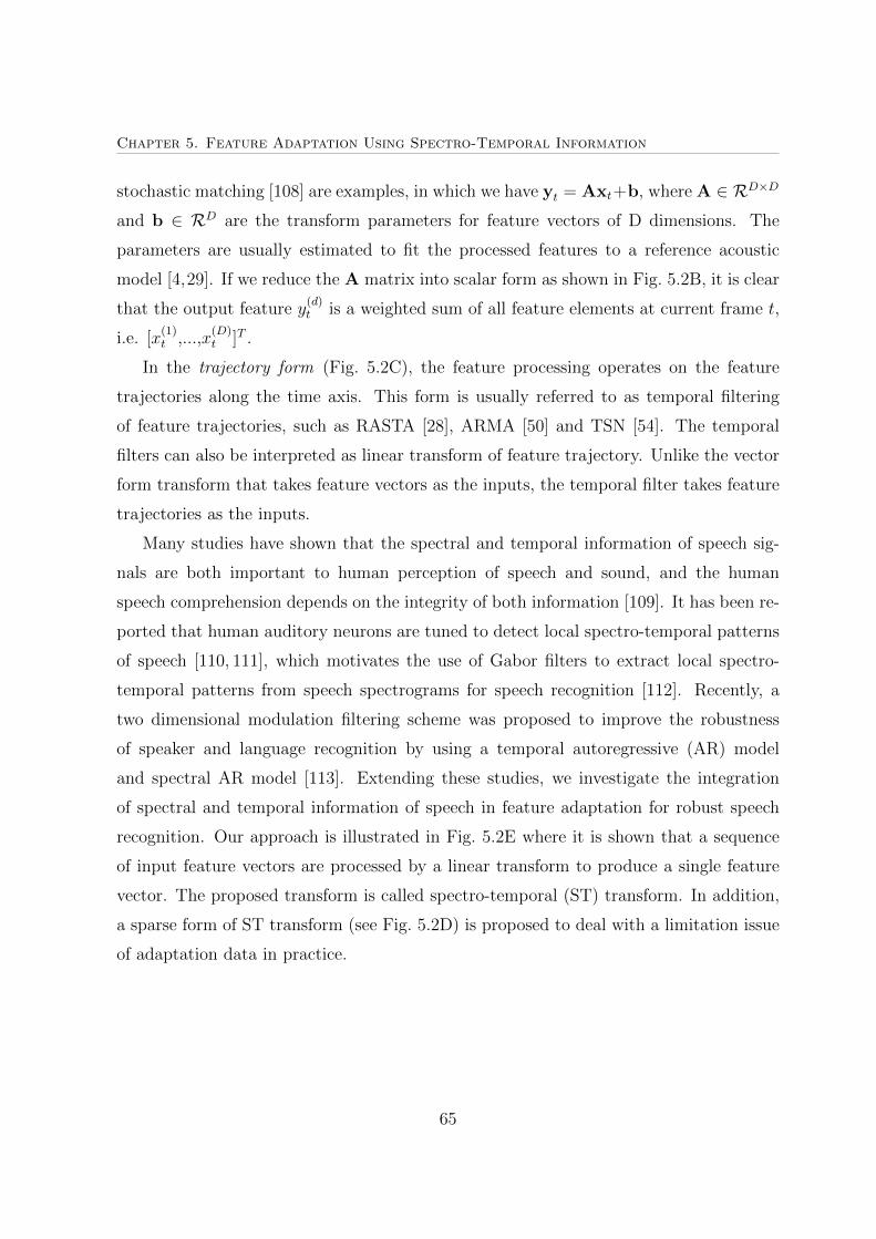
Chapter 5. Feature Adaptation Using Spectro-Temporal Information
stochastic matching [108] are examples, in which we have yt = Axt+b, where A ∈ RD×D
and b ∈ RD are the transform parameters for feature vectors of D dimensions. The
parameters are usually estimated to fit the processed features to a reference acoustic
model [4,29]. If we reduce the A matrix into scalar form as shown in Fig. 5.2B, it is clear
that the output feature y(d)t is a weighted sum of all feature elements at current frame t,
i.e. [x(1)t ,...,x
(D)t ]T .
In the trajectory form (Fig. 5.2C), the feature processing operates on the feature
trajectories along the time axis. This form is usually referred to as temporal filtering
of feature trajectories, such as RASTA [28], ARMA [50] and TSN [54]. The temporal
filters can also be interpreted as linear transform of feature trajectory. Unlike the vector
form transform that takes feature vectors as the inputs, the temporal filter takes feature
trajectories as the inputs.
Many studies have shown that the spectral and temporal information of speech sig-
nals are both important to human perception of speech and sound, and the human
speech comprehension depends on the integrity of both information [109]. It has been re-
ported that human auditory neurons are tuned to detect local spectro-temporal patterns
of speech [110, 111], which motivates the use of Gabor filters to extract local spectro-
temporal patterns from speech spectrograms for speech recognition [112]. Recently, a
two dimensional modulation filtering scheme was proposed to improve the robustness
of speaker and language recognition by using a temporal autoregressive (AR) model
and spectral AR model [113]. Extending these studies, we investigate the integration
of spectral and temporal information of speech in feature adaptation for robust speech
recognition. Our approach is illustrated in Fig. 5.2E where it is shown that a sequence
of input feature vectors are processed by a linear transform to produce a single feature
vector. The proposed transform is called spectro-temporal (ST) transform. In addition,
a sparse form of ST transform (see Fig. 5.2D) is proposed to deal with a limitation issue
of adaptation data in practice.
65

Chapter 5. Feature Adaptation Using Spectro-Temporal Information
Figure 5.3: An illustration of the Spectro-Temporal feature transform, or ST transform,in Eq 5.1.
5.2 Generalized Linear Transform for Feature Adap-
tation
ASR performance degrades in face of mismatch between the training and test features.
Mismatch may occur due to various reasons, such as speaker variation, background noise,
reverberation, and transmission channel. One way to reduce mismatch is to adapt the
statistics of test features towards those of training features. Examples of this approach
include CMN, MVN, HEQ, and fMLLR. We now study a generalized linear feature trans-
form for feature adaptation. The transform is illustrated in Fig. 5.3 and called ST trans-
form. Mathematically, ST transform is defined as follows:
yt =L∑
τ=−L
Aτxt+τ + b = Wxt (5.1)
where xt and yt are the input and output feature vectors at frame t, respectively. Aτ
(with τ = −L, . . . , L) is a sequence of transform matrices over 2L+ 1 frames. b is a bias
vector. ST transform can therefore be viewed as a linear transform over a supervector of
2L + 1 stacked feature vectors xt = [xTt−L, ...,xTt+L, 1]T with a transform matrix (or the
general transform matrix) W = [A−L, ...,AL,b] as shown in Fig 5.3.
Note that ST transform in (5.1) is the most general form of linear processing of
features. Both fMLLR and temporal filters are special cases of (5.1). Specifically, when
66
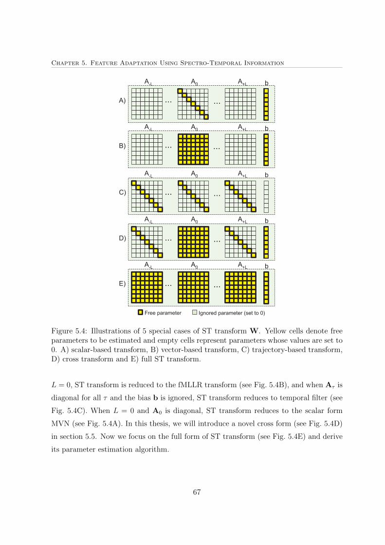
Chapter 5. Feature Adaptation Using Spectro-Temporal Information
Figure 5.4: Illustrations of 5 special cases of ST transform W. Yellow cells denote freeparameters to be estimated and empty cells represent parameters whose values are set to0. A) scalar-based transform, B) vector-based transform, C) trajectory-based transform,D) cross transform and E) full ST transform.
L = 0, ST transform is reduced to the fMLLR transform (see Fig. 5.4B), and when Aτ is
diagonal for all τ and the bias b is ignored, ST transform reduces to temporal filter (see
Fig. 5.4C). When L = 0 and A0 is diagonal, ST transform reduces to the scalar form
MVN (see Fig. 5.4A). In this thesis, we will introduce a novel cross form (see Fig. 5.4D)
in section 5.5. Now we focus on the full form of ST transform (see Fig. 5.4E) and derive
its parameter estimation algorithm.
67
Chapter 5. Feature Adaptation Using Spectro-Temporal Information
5.3 Review of Maximum Likelihood Based Feature
Adaptation
Maximum likelihood (ML) criterion is widely used to estimate the transformation matrix
of a feature vector (we will later call this the square transform in view of the shape of
the transform matrix). In this section, we review the ML criterion and point out the
difficulty of directly applying it to estimate a general transformation matrix of several
consecutive feature vectors (we will call this corresponding transform the rectangular
transform).
Without loss of generality, we take the feature transform for speech denoising as an
example to illustrate the ML criterion. Let’s assume that the noise corruption process can
be approximated by an invertible linear transform, and the observed noisy feature vector
can be represented as y = Ax and x is the unobserved clean feature vector. If we know
the probability density function (PDF) of the clean features f(x), e.g. from an acoustic
model, we can obtain the PDF of the corrupted features g(y) directly by applying the
change of variables formula [114], i.e. g(y) = f(x)| det(dx/dy)| = f(x)| det(A−1)|, where
x = A−1y. In practice, the inverse transform A−1 is estimated such that the likelihood of
the observed noisy features is maximum when evaluted on g(y). Then we can apply the
estimated transform A−1 to reverse the corruption process and adapt the noisy feautres
towards the clean model by using x = A−1y. For square transform such as stochastic
matching [108] and fMLLR [4], it is straightforward to apply the ML criterion to estimate
the transform, as the determinant of a square matrix can be computed.
If the transform is not square, there will be difficulty in directly using the ML frame-
work as the determinant of the Jacobian matrix does not exist and the transform is not
invertible. This is the case when we project a sequence of feature vectors to a single fea-
ture vector and the transform is a D ×M matrix where D < M . In the studies of [115]
and DCMLLR [10], instead of estimating a rectangular transform, a square transform
of size M ×M is estimated by using the ML criterion but the last M − D rows of the
transform are discarded. The discarded dimensions are modeled by a single Gaussian
for all phone classes, hence all discriminative information are pushed into the the first D
dimensions of the projected space. The tying of all phone classes to a single Gaussian for
68
Chapter 5. Feature Adaptation Using Spectro-Temporal Information
discarded dimensions is conceptually the same as the tying used in HLDA [116], hence
this kind of transform can be seen as the speaker dependent HLDA transform [115].
However, a potential drawback of this appraoch is that the computational cost of trans-
form estimation may be high for large M , and most of the rows of the transform will be
discarded.
To avoid estimating a full square transform, one can use a technique called Jacobian
compensation which replaces the Jacobian term of the ML objective function with the
determinant of the sample covariance matrix of the transformed features. This method
has been used in transforms where no theorectial Jacobian can be computed. For exam-
ple, it is used in vocal tract length normalization (VTLN) [117] to correct the systematic
error in choosing the warping factor.
In the following section, we propose a new objective function for feature adapta-
tion based on minimizing the Kullback-Leibler (KL) divergence between two distribution
functions, i.e. the transformed features’ sample distribution and the acoustic model. We
will show that under certain assumptions, the KL divergence objective function will lead
to the objective function of ML criterion with Jacobian compensation. We will also pro-
vide an expectation-maximization (EM) based method for iteratively estimating the ST
transform parameters.
5.4 Minimum Kullback-Leibler (KL) Divergence Cri-
terion
5.4.1 Objective function
The ST transform W is estimated to minimize a KL divergence [118, 119] between the
distribution of the transformed features, py, and the reference distribution of the training
features, parameterized as pΛ. The reference distribution can be of any form, such as
a GMM, to represent the distribution of the training data. We have the following KL
divergence [119],
DKL (py||pΛ) =
∫y
py(y) logpy(y)
pΛ(y)dy = −H(py) +H(py, pΛ) (5.2)
69
Chapter 5. Feature Adaptation Using Spectro-Temporal Information
where
H(py) = −∫
y
py(y) log(py(y))dy (5.3)
is the entropy of distribution py, and
H(py, pΛ) = −∫
y
py(y) log pΛ(y)dy (5.4)
is the cross entropy of py and pΛ. As y is determined by W through (5.1), the trans-
form matrix W can be estimated by minimizing DKL (py||pΛ) such that the transformed
features will have distribution closer to that of the reference.
To evaluate (5.2), we need some run-time adaptation data from the test environment.
If such data are limited, it is a challenge to reliably characterize the test environment.
Under such condition, we choose to approximate py(y) as a single Gaussian distribution
with full covariance matrix. In this way, H(py) can be shown to depend only on the
determinant of the covariance matrix Σy as follows
H(py) ≈ K +1
2log |Σy| (5.5)
where K is a constant. In practice, the covariance matrix is estimated from the available
run-time adaptation data.
The second term H(py, pΛ) in (5.2) specifies the cross entropy between py and pΛ.
One way to evaluate this term is to use a Gaussian approximation of py. However, this
doesn’t provide an easy solution to the optimization of KL divergence function. Instead,
we use Monte Carlo approximation, i.e. we use the available adaptation feature vectors
as random samples drawn from the distribution py and evaluate the cross-entropy by
H(py, pΛ) ≈ −T∑t=1
1
Tlog(pΛ(yt)) (5.6)
where the integration over y in (5.2) is replaced with summation over adaptation feature
vectors yt and T is the number of available adaptation feature vectors. The equation
(5.6) is the negative average log likelihood of the transformed features evaluated in the
reference feature distribution function.
70
Chapter 5. Feature Adaptation Using Spectro-Temporal Information
With the approximation of H(py) in (5.5) and H(py, pΛ) in (5.6), the KL divergence
can be rewritten as
DKL (py||pΛ) ≈ −K − 1
2log |Σy| −
1
T
T∑t=1
log(pΛ(yt)) (5.7)
In this way, we are actually maximizing both the log likelihood of the transformed features
on reference feature distribution as well as the log determinant of the transformed features
covariance matrix.
The reference distribution pΛ can be any distribution function of training speech
features. Here, we use a GMM with diagonal covariance matrices for simplicity. A GMM
of M Gaussians is defined by a set of parameters {cm,µm,Σm}, i.e.
pΛ(yt) =M∑m=1
cmN (yt;µm,Σm) (5.8)
where µm and Σm are the mean and diagonal covariance matrix of the mth Gaussian
component. The parameters of GMM can be estimated from training data. With this
definition of pΛ(yt), the KL divergence in (5.7) can be rewritten as
DKL(py||pΛ) ≈ −K − 1
2log |Σy|
− 1
T
T∑t=1
log
(M∑m=1
cmN (yt;µm,Σm)
)(5.9)
Applying (5.9), we propose to estimate ST transform by
W = arg minW
f(W) (5.10)
where the cost function is defined as:
f(W) =β
2T||W−W0||2F −
λ
2log |Σy|
− 1
T
T∑t=1
log
(M∑m=1
cmN (yt;µm,Σm)
)(5.11)
The above cost function includes the KL divergence as well as a Frobenius matrix norm
term (also called L2 norm term) ||W −W0||2F to regulate the transform. W0 is the
initial parameters of the transform, in which b and Aτ in (5.1) contain all zero’s for
71
Chapter 5. Feature Adaptation Using Spectro-Temporal Information
Table 5.1: Estimation of W to minimize the cost function in (5.11)
Step 1: Set W = W0.Step 2: Compute statistics in (5.15) first, then (5.13) and (5.14).Step 3: Estimate W to minimize Q(W,W) in (5.12).
using L-BFGS algorithm [120] with gradient defined in (5.16).Step 4: If convergence is met or maximum number of iterations
is reached, exit.Otherwise set W = W and go to Step 2.
τ 6= 0 and A0 is the identity matrix. With this design, W0xt = xt. With the L2 term,
the transformed features are ensured to be not too far from the initial features if W
is near to W0 in the parameter space. The parameters β and λ are tunable and used
to control the contributions of the Frobenius norm and data distribution py in the cost
function, respectively. Note that if λ = 1, the term 12
log |Σy| is the same as the Jacobian
compensation used in VTLN [117].
The objective function in (5.11) contains two terms that pull the transform estimation
in opposite directions. On one hand, the log likelihood term fits the transformed features
to the means of Gaussians that are originally close to the observed features. Hence it will
tend to shrink the variances of the transformed features and make py cover only a fraction
of the acoustic space of pΛ. On the other hand, the log determinant term is trying to
spread py so it can cover a larger part of the acoustic space. The optimal solution of the
transform is a tradeoff between these two factors.
5.4.2 EM Algorithm for Parameter Estimation
There is no closed form solution for the minimization problem in (5.11) due to the hidden
variables of the Gaussian occupancy in the GMM. We use an EM algorithm [44] to search
for a locally optimal solution iteratively. The EM algorithm is an effective method for
estimation problems with incomplete data such as (5.11). The auxiliary function of the
72
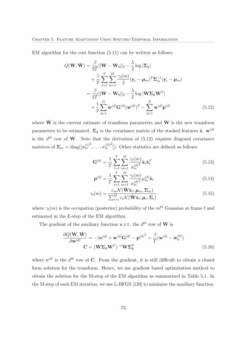
Chapter 5. Feature Adaptation Using Spectro-Temporal Information
EM algorithm for the cost function (5.11) can be written as follows:
Q(W,W) =β
2T||W−W0||2 −
λ
2log |Σy|
+1
T
T∑t=1
M∑m=1
γt(m)
2(yt − µm)TΣ−1
m (yt − µm)
=β
2T||W−W0||2 −
λ
2log |WΣxWT |
+1
2
D∑d=1
w(d)G(d)(w(d))T −D∑d=1
w(d)p(d) (5.12)
where W is the current estimate of transform parameters and W is the new transform
parameters to be estimated. Σx is the covariance matrix of the stacked features x. w(d)
is the dth row of W. Note that the derivation of (5.12) requires diagonal covariance
matrices of Σm = diag([σ(1)m
2, . . . , σ
(D)m
2]). Other statistics are defined as follows:
G(d) =1
T
T∑t=1
M∑m=1
γt(m)
σ(d)m
2 xtxTt (5.13)
p(d) =1
T
T∑t=1
M∑m=1
γt(m)
σ(d)m
2 µ(d)m xt (5.14)
γt(m) =cmN (Wxt;µm,Σm)∑Mi=1 ciN (Wxt;µi,Σi)
(5.15)
where γt(m) is the occupation (posterior) probability of the mth Gaussian at frame t and
estimated in the E-step of the EM algorithm.
The gradient of the auxiliary function w.r.t. the dth row of W is
∂Q(W,W)
∂w(d)= −λc(d) + w(d)G(d) − p(d)T +
β
T(w(d) −w
(d)0 )
C = (WΣxWT )−1WΣTx (5.16)
where c(d) is the dth row of C. From the gradient, it is still difficult to obtain a closed
form solution for the transform. Hence, we use gradient based optimization method to
obtain the solution for the M-step of the EM algorithm as summarized in Table 5.1. In
the M step of each EM iteration, we use L-BFGS [120] to minimize the auxiliary function.
73
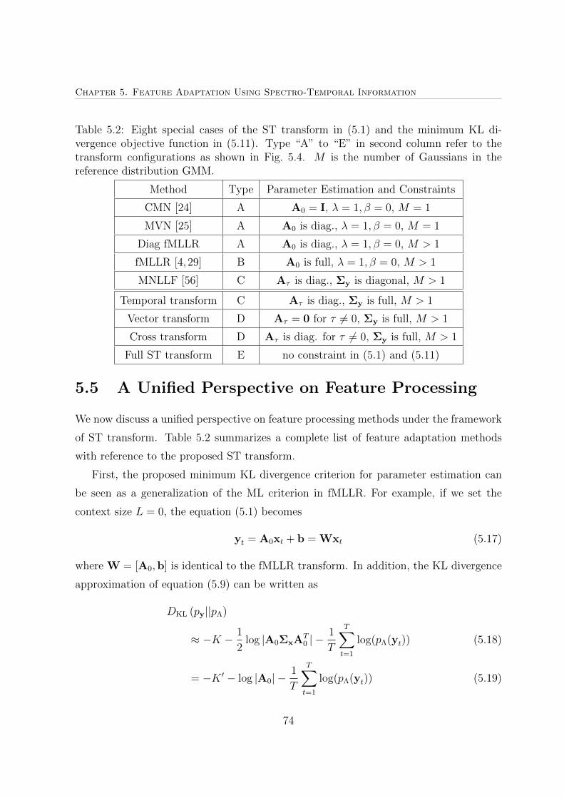
Chapter 5. Feature Adaptation Using Spectro-Temporal Information
Table 5.2: Eight special cases of the ST transform in (5.1) and the minimum KL di-vergence objective function in (5.11). Type “A” to “E” in second column refer to thetransform configurations as shown in Fig. 5.4. M is the number of Gaussians in thereference distribution GMM.
Method Type Parameter Estimation and Constraints
CMN [24] A A0 = I, λ = 1, β = 0, M = 1
MVN [25] A A0 is diag., λ = 1, β = 0, M = 1
Diag fMLLR A A0 is diag., λ = 1, β = 0, M > 1
fMLLR [4,29] B A0 is full, λ = 1, β = 0, M > 1
MNLLF [56] C Aτ is diag., Σy is diagonal, M > 1
Temporal transform C Aτ is diag., Σy is full, M > 1
Vector transform D Aτ = 0 for τ 6= 0, Σy is full, M > 1
Cross transform D Aτ is diag. for τ 6= 0, Σy is full, M > 1
Full ST transform E no constraint in (5.1) and (5.11)
5.5 A Unified Perspective on Feature Processing
We now discuss a unified perspective on feature processing methods under the framework
of ST transform. Table 5.2 summarizes a complete list of feature adaptation methods
with reference to the proposed ST transform.
First, the proposed minimum KL divergence criterion for parameter estimation can
be seen as a generalization of the ML criterion in fMLLR. For example, if we set the
context size L = 0, the equation (5.1) becomes
yt = A0xt + b = Wxt (5.17)
where W = [A0,b] is identical to the fMLLR transform. In addition, the KL divergence
approximation of equation (5.9) can be written as
DKL (py||pΛ)
≈ −K − 1
2log |A0ΣxAT
0 | −1
T
T∑t=1
log(pΛ(yt)) (5.18)
= −K ′ − log |A0| −1
T
T∑t=1
log(pΛ(yt)) (5.19)
74
Chapter 5. Feature Adaptation Using Spectro-Temporal Information
where we have used the property that Σy = A0ΣxAT0 when L = 0. The divergence func-
tion in (5.19) is actually the negative of the log likelihood objective function of fMLLR.
Hence, fMLLR is a special case of ST transform without using the contextual frames.
With reference to the original fMLLR algorithm, the EM algorithm described in Sec-
tion 5.4.2 has several different properties, i.e. tunable contribution from log determinant
of linear transform matrix and the use of L2 norm. The use of L2 norm has similar
effect as imposing a Gaussian prior distribution on the transform parameters and is ex-
pected to perform similarly with feature space maximum a posteriori linear regression
(fMAPLR) [121].
Second, ST transform can also be seen as a generalization of temporal filters, such
as MNLLF [56]. In MNLLF filters, the feature trajectories are filtered separately. In ST
transform, all the feature trajectories are filtered simultaneously.
5.6 Implementation Issues
In this section, we will discuss several practical issues in implementing ST transform. In
particular, the estimation of parameters given limited adaptation data. We will discuss
3 approaches to address this issue: 1) sparse ST transform; 2) cascaded transforms; 3)
regularization and statistics smoothing.
5.6.1 Sparse Generalized Linear Transform
ST transform in its full capacity is characterized by a large set of parameters, that requires
a large number of training data. For example, If L = 10, i.e. we use a context of 21
feature vectors centred at the current frame, there will be 39 × 39 × 21 + 39 = 31, 980
parameters. It is very difficult, if not impossible, to reliably estimate such a large amount
of parameters from a few seconds of speech. Hence, it is necessary to reduce the number
of parameters in ST transform.
One way to reduce the number of parameters is to force some parameters to be zero
and make the transform matrices Aτ sparse. From Eq. (5.1), each element of the adapted
feature vector is a linear weighted sum of all the feature elements in the neighboring
frames. It is reasonable to believe that not all elements of the spectro-temporal context
75
Chapter 5. Feature Adaptation Using Spectro-Temporal Information
are equally important for predicting a feature element. By setting the parameters of the
less important context zero, we reduce the number of free parameters and estimate the
effective parameters more reliably.
In this study, we consider 3 types of sparse transforms as illustrated in Fig. 5.4B,
5.4C and 5.4D. In the first simplification, we set the parameters of feature elements in
neighboring frames to zero, i.e. Aτ = 0 except for τ = 0 (see Fig. 5.4B) and Table 5.2.
In this way, only the spectral information of the current frame is used, and the number
of free parameters is reduced to D(D+ 1). This simplification of the ST transform turns
out to be the popular fMLLR transform.
In the second simplification, we set the parameters of the feature trajectories other
than the current one to zero, i.e. Aτ is set to diagonal for −L ≤ τ ≤ L (see Fig. 5.4C)
and Table 5.2. In this case, only temporal information in the current feature trajectory is
used for feature adaptation, and the number of free parameters is reduced to D(2L+ 1).
This simplification leads to temporal filtering of features. We have studied this type
of sparse transform in [56] and found it useful for dealing with reverberation. We note
that the two simplifications above do not make use of spectral and temporal information
simultaneously.
From fMLLR, we know that single frame spectral information allows us to handle
short term feature variations such as speaker variation and additive noise distortions.
From temporal filter, we learn that the temporal trajectory of a feature element along
the time axis removes long term variation such as reverberation. Hence, we propose
the third sparse transform that benefits from the best of both fMLLR transform and
temporal filter. In particular, we restrict Aτ in (5.1) to be diagonal for τ 6= 0 to capture
the temporal information, while keeping A0 as a full matrix to incorporate the spectral
information of current frame. With the new transform in Fig. 5.4D, the number of free
parameters is reduced significantly, while both spectral and temporal information can be
partially modeled. Specifically, the ratio of free parameters of the new design over the
full ST transform is 2LD+D2+D2LD2+D2+D
= 2L+D+12LD+D+1
. For example, with L = 10 and D = 39, the
ratio is 2×10+39+12×10×39+39+1
= 60820≈ 7%. Examining Fig. 5.2D and Fig. 5.4D, we find that such
a transform practically applies a cross-shape mask on the features, hence, we call it the
cross transform.
76
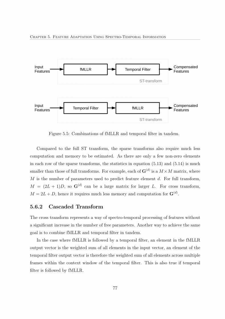
Chapter 5. Feature Adaptation Using Spectro-Temporal Information
fMLLR Temporal FilterInput Features
Compensated Features
ST-transform
Temporal Filter fMLLRInput Features
Compensated Features
ST-transform
Figure 5.5: Combinations of fMLLR and temporal filter in tandem.
Compared to the full ST transform, the sparse transforms also require much less
computation and memory to be estimated. As there are only a few non-zero elements
in each row of the sparse transforms, the statistics in equation (5.13) and (5.14) is much
smaller than those of full transforms. For example, each of G(d) is a M×M matrix, where
M is the number of parameters used to predict feature element d. For full transform,
M = (2L + 1)D, so G(d) can be a large matrix for larger L. For cross transform,
M = 2L+D, hence it requires much less memory and computation for G(d).
5.6.2 Cascaded Transform
The cross transform represents a way of spectro-temporal processing of features without
a significant increase in the number of free parameters. Another way to achieve the same
goal is to combine fMLLR and temporal filter in tandem.
In the case where fMLLR is followed by a temporal filter, an element in the fMLLR
output vector is the weighted sum of all elements in the input vector, an element of the
temporal filter output vector is therefore the weighted sum of all elements across multiple
frames within the context window of the temporal filter. This is also true if temporal
filter is followed by fMLLR.
77
Chapter 5. Feature Adaptation Using Spectro-Temporal Information
If we consider the full ST transform as a 2-dimensional filtering of the time-quefrency1
representation of the speech (e.g. cepstral features), then fMLLR and temporal filter can
be seen as 1-dimensional filters, one along the quefrency axis and the other along the
time axis. Applying the two 1-dimensional filters in sequence will be effectively the same
as applying a 2-dimensional filtering with its weight matrix having a rank of 1. The
advantage of such cascaded transform is that it has a much fewer number of parameters
and require much less memory and computation to estimate than the full ST transform.
It would be intereting to see how such cascaded transform perform against the full ST
transform and cross transform.
5.6.3 Interpolation of Statistics
With fewer number of parameters, cross transform and cascaded transform are expected
to work better than full ST transform given a limited amount of data. However, in many
applications, the adaptation data are the test sentence itself which is of several seconds
in length. In such cases, it is even difficult to estimate the fMLLR or temporal filters.
To address this issue, we apply L2 norm regularization on the parameters and smoothing
of the sufficient statistics in the EM algorithm. The L2 norm regularization was already
introduced in (5.11) as the Frobenius norm. Next we discuss how the statistics smoothing
works.
The EM algorithm for transform estimation relies on several sufficient statistics such
as the mean vector and covariance matrix of the input feature vectors, the G(d) and
p(d) for all dimensions as defined in (5.13) and (5.14). Generally speaking, if the test
environment is stable, more adaptation data will result in more reliable estimation of
these statistics, which will in turn lead to better adapted features. The idea of statistics
smoothing is to interpolate the statistics computed from the adaptation data with the
statistics computed from some prior data in the following way:
G(d)
= αG(d,0) + (1− α)G(d) (5.20)
p(d) = αp(d,0) + (1− α)p(d) (5.21)
1Assuming we are applying the transforms on cepstral features, one dimension of the feature repre-sentation is time and the other is quefrency.
78
Chapter 5. Feature Adaptation Using Spectro-Temporal Information
where G(d,0) and p(d,0) are prior statistics computed from prior data; and G(d) and p(d)
are statistics computed from adaptation/test data. The tunable parameter α is used
to control the level of smoothing; i.e. if α = 0, the smoothing will be ignored, while
α = 1 will ignore the contribution from the adaptation data. Similar statistics smooth-
ing approach have been proposed for fMLLR in [122–124]. In addition, the mean and
covariance matrix of extended features x can also be approximated as in [125]
µx = αµ(0)x + (1− α)µx (5.22)
Σx = E(xxT )− µxµTx (5.23)
E(xxT ) = αE(0)xx +
(1− α)
T
T∑t=1
xtxTt (5.24)
where µ(0)x and E
(0)xx are the prior expected values of x and xxT and computed from
the prior data. µx is the expected value of x, computed from adaptation/test data. In
practice, the prior data can be the training data, or development data that are from
similar environment as the test data.
5.7 Experimental Study on Spectro-Temporal Trans-
form
5.7.1 Experimental Settings
5.7.1.1 Task Description
To further understand the ST transform, we conduct experiments on the REVERB Chal-
lenge 2014 benchmark task for noisy and reverberant speech recognition [126]. We focus
on using clean condition training scheme, in which we assume that only clean speech
data are available at system training stage whereas test data are noisy and reverber-
ant. This task has the most mismatch between training and testing data. Due to the
mismatch, performance of ASR system will be degraded dramatically if no adaptation
or compensation method is applied. This chapter will compare the improvement of the
ASR system by using feature adaptation with the ST transform, its variations and other
relative transforms such as fMLLR.
79
Chapter 5. Feature Adaptation Using Spectro-Temporal Information
In the clean condition training scheme, the training data consist of 7,861 clean ut-
terances (about 17.5 hours from 92 speakers) from the WSJCAM0 database [127]. The
clean data are recorded in a quiet room using a head-mounted close-talking microphone
(Sennheiser HMD414-6).
In this work, a baseline ASR system is based on a triphone-based HMM/GMM acous-
tic model. The context-dependent triphone models are clustered into 3,115 tied states and
10 Gaussians are used to model the feature distribution of each tied state. Mel-frequency
cepstral coefficients (MFCC) are used as acoustic features with utterancewise MVN post-
processing if not otherwise specified. Particularly, the first 13 (c0-c12) MFCCs and their
first and second derivatives are extracted from each 25ms frame with 10ms hopping time.
Hence, the frame rate is 100 frames per second. The features of every utterance are then
normalized to zero mean and unit variances. The word error rate (WER) on clean test
set is about 12.3%, which is the lower bound to achieve by adapting the features of noisy
and reverberant speech.
The development (dev) and evaluation (eval) data sets are taken from actual meeting
room recording of MC-WSJ-AV [128]. The dev and eval sets are similar to each other in
terms of noise and reverberation characteristics. For either dev and eval sets, the data
are divided into two subsets according to the distance between the microphone and the
speaker, i.e. near subset with a distance of 100cm and far subset with a distance of
250cm. The reverberation time T60 for the meeting room is about 0.7s. There are totally
179 utterances (about 0.3 hour and from 10 speakers) in the dev set and 372 utterances
(about 0.6 hour and from 20 speakers) in the eval set. For more details of the REVERB
Challenge 2014 task, the readers are referred to [126].
5.7.1.2 Feature Adaptation Schemes
We evaluate four types of linear transforms for feature adaptation against reverberation
and noise distortions in ASR experiments, including fMLLR, temporal filter, cross trans-
form, and full ST transform. We also test the cascading of these transforms, for example,
“fMLLR ◦ Temporal” represents fMLLR followed by temporal filters. The ◦ operator
is used to denote the fact that combination “fMLLR ◦ Temporal” will generate a ST
transform whose transform matrix is of rank 1. These transforms are implemented under
80
Chapter 5. Feature Adaptation Using Spectro-Temporal Information
the same framework of the EM algorithm in Table 5.1 and estimated separately. The
number of EM-iterations is set to 10 except for multi-condition training whose settings
will be explained later. The Jacobian weight λ is set to 1 in all the experiments. The
context size L is set to 10 for temporal, cross and full transforms unless otherwise stated.
The L2 norm weight β is tuned according to the development data.
We also carry out experiments with four different adaptation schemes, including full
batch mode, speaker mode, utterance mode, and hybrid mode. In the full batch mode,
one feature transform (e.g. temporal filter, fMLLR, cross or full ST transform) is esti-
mated for each setting of the microphone distances. In the real eval set, each microphone
distance contains about 180 utterances and the average utterance length is 7 seconds
including silence. With that, we suppose that we have sufficient adaptation data to
estimate most of the transforms under study.
In the speaker mode, one feature transform is estimated for each test speaker and dis-
tance combination. There are about 18 utterances for each speaker on average. Although
the speaker mode has less adaptation data per transform than the full batch mode, it
allows the adaptation of features to reduce speaker variations.
In the utterance mode, one feature transform is estimated for each test utterance.
As each utterance is only about 7s long on average, it is a challenge to estimate most of
the feature transforms. We don’t try the full ST transform here due to its large amount
of parameters. An advantage of utterance mode processing is that the features can be
adapted to address both speaker variation and small variations of reverberant distortions
across utterances.
In the hybrid mode, we estimate the utterance based transform and smooth the suffi-
cient statistics between the utterance based statistics and the full batch mode statistics.
In this way, we expect more reliable estimation yet we are able to follow the reverberation
change from utterance to utterance.
5.7.1.3 Feature Adaptation Reference Model
A reference model pΛ in (5.7) is required to describe the distribution of the training
features for the estimation of feature transform parameters. In theory, the HMM/GMM
based acoustic model can be used as a reference model. However, it requires two-pass
81
Chapter 5. Feature Adaptation Using Spectro-Temporal Information
decoding: the first pass generates the hypotheses from which we obtain the Gaussian
occupancy probabilities γt(m) for estimating feature transforms, and the second pass
generates the final recognition output using the transformed features. As decoding is time
consuming, we choose to use a simple GMM as the reference model for feature adaptation.
For GMM, the Gaussian occupancy probabilities can be readily computed efficiently
once the feature vector is observed. This allows us to perform multiple iterations of EM
algorithm, in each iteration the Gaussian occupancy probabilities are updated using the
latest transformed features. A GMM reference model that contains 4,416 Gaussians is
obtained by pooling the Gaussians from a monophone-based HMM/GMM model. As
both the GMM and HMM/GMM are trained from the same clean training corpus, if the
distribution of the transformed features matches the GMM well, it is also expected to
match the HMM/GMM reasonably well.
5.7.2 Effect of Window Length L
One of the most important considerations in ST transform is the context window size
which is equal to 2L+ 1. We report the effect of window size on the development data in
Fig. 5.6. All transforms are estimated in the full batch mode, i.e. one feature transform is
estimated for each setting of the microphone distances. From the figure, we can see that
all transforms that explicitly use temporal information, including temporal filter, cross
transform, and the full ST transform, produces lower WER as the windowsize increases.
At window length of 1 frame, the full transform, cross transform, and fMLLR have the
same performance as they are exactly the same. However, the temporal filter and MVN
give different results when window size is 1 although they have the same scalar form.
This is because MVN is equivalent to using a single Gaussian as a reference model, while
temporal filter using a GMM of 4,416 Gaussians as reference model.
The performance saturates at around 21 frames or L = 10, across the board. The
window length of 21 frames corresponds to about 0.3s of temporal information with a
frame rate of 100Hz if we also include the temporal information in the dynamic features.
For comparison, the fMLLR only uses temporal information up to 0.1s through the
dynamic features. The results show that long term temporal information (>0.1s) is
useful for feature adaptation to improve robustness of ASR system against reverberation
82
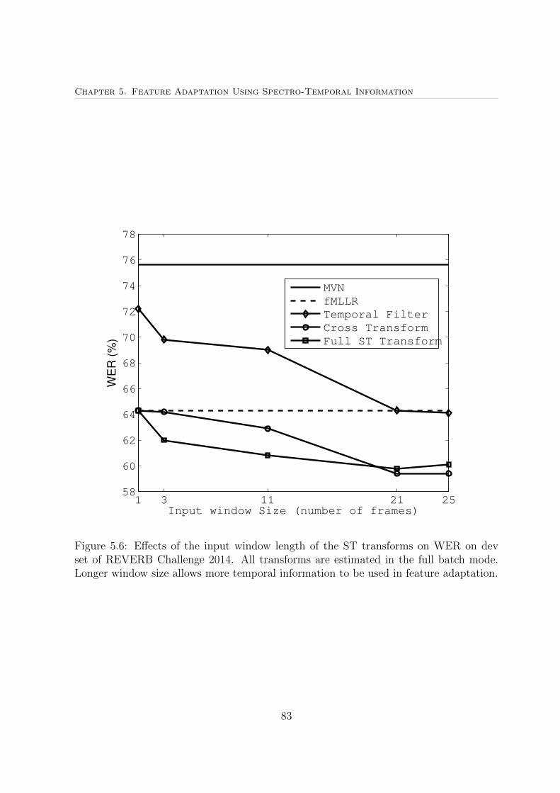
Chapter 5. Feature Adaptation Using Spectro-Temporal Information
1 3 11 21 2558
60
62
64
66
68
70
72
74
76
78
Input window Size (number of frames)
WE
R (
%)
MVN
fMLLR
Temporal Filter
Cross Transform
Full ST Transform
Figure 5.6: Effects of the input window length of the ST transforms on WER on devset of REVERB Challenge 2014. All transforms are estimated in the full batch mode.Longer window size allows more temporal information to be used in feature adaptation.
83
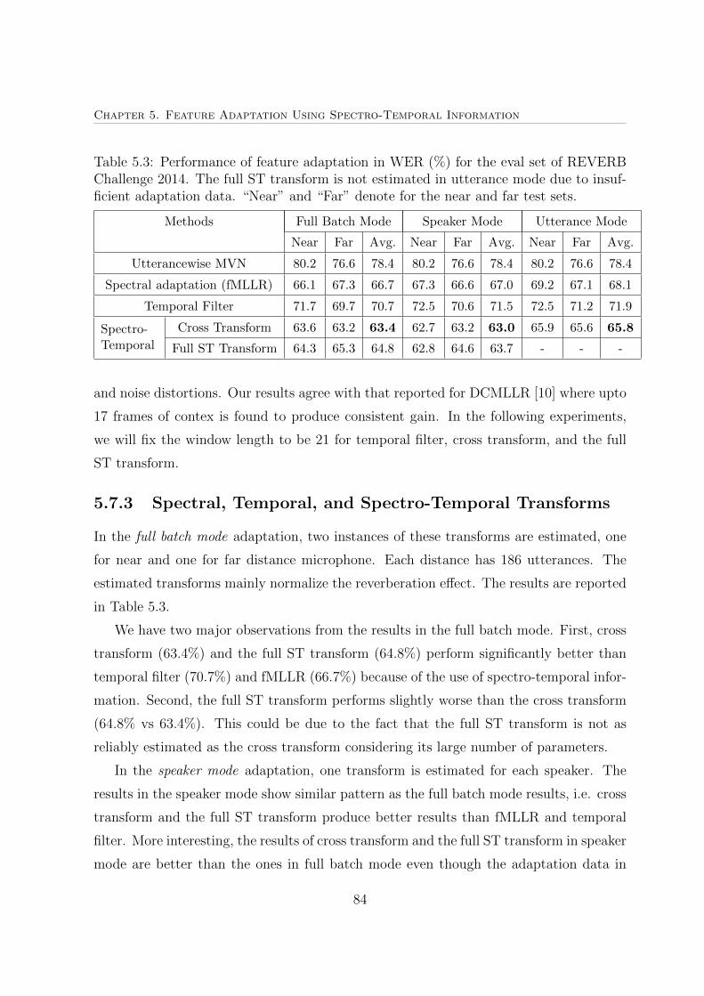
Chapter 5. Feature Adaptation Using Spectro-Temporal Information
Table 5.3: Performance of feature adaptation in WER (%) for the eval set of REVERBChallenge 2014. The full ST transform is not estimated in utterance mode due to insuf-ficient adaptation data. “Near” and “Far” denote for the near and far test sets.
Methods Full Batch Mode Speaker Mode Utterance Mode
Near Far Avg. Near Far Avg. Near Far Avg.
Utterancewise MVN 80.2 76.6 78.4 80.2 76.6 78.4 80.2 76.6 78.4
Spectral adaptation (fMLLR) 66.1 67.3 66.7 67.3 66.6 67.0 69.2 67.1 68.1
Temporal Filter 71.7 69.7 70.7 72.5 70.6 71.5 72.5 71.2 71.9
Spectro-Temporal
Cross Transform 63.6 63.2 63.4 62.7 63.2 63.0 65.9 65.6 65.8
Full ST Transform 64.3 65.3 64.8 62.8 64.6 63.7 - - -
and noise distortions. Our results agree with that reported for DCMLLR [10] where upto
17 frames of contex is found to produce consistent gain. In the following experiments,
we will fix the window length to be 21 for temporal filter, cross transform, and the full
ST transform.
5.7.3 Spectral, Temporal, and Spectro-Temporal Transforms
In the full batch mode adaptation, two instances of these transforms are estimated, one
for near and one for far distance microphone. Each distance has 186 utterances. The
estimated transforms mainly normalize the reverberation effect. The results are reported
in Table 5.3.
We have two major observations from the results in the full batch mode. First, cross
transform (63.4%) and the full ST transform (64.8%) perform significantly better than
temporal filter (70.7%) and fMLLR (66.7%) because of the use of spectro-temporal infor-
mation. Second, the full ST transform performs slightly worse than the cross transform
(64.8% vs 63.4%). This could be due to the fact that the full ST transform is not as
reliably estimated as the cross transform considering its large number of parameters.
In the speaker mode adaptation, one transform is estimated for each speaker. The
results in the speaker mode show similar pattern as the full batch mode results, i.e. cross
transform and the full ST transform produce better results than fMLLR and temporal
filter. More interesting, the results of cross transform and the full ST transform in speaker
mode are better than the ones in full batch mode even though the adaptation data in
84
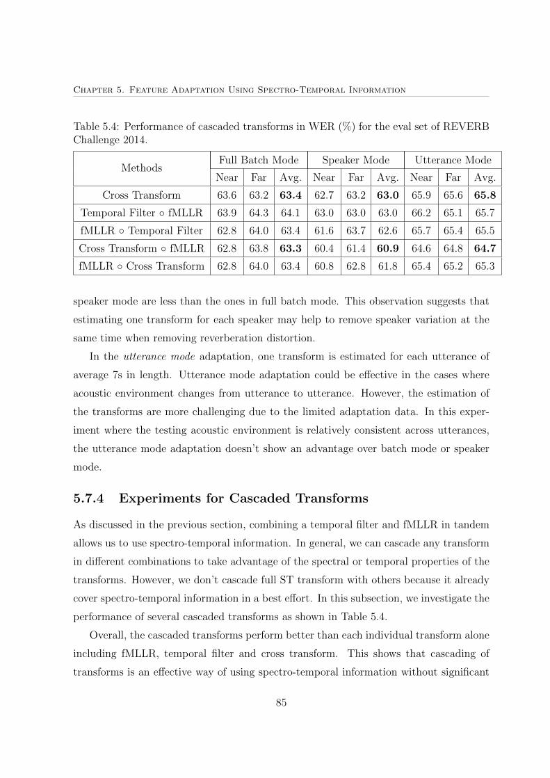
Chapter 5. Feature Adaptation Using Spectro-Temporal Information
Table 5.4: Performance of cascaded transforms in WER (%) for the eval set of REVERBChallenge 2014.
MethodsFull Batch Mode Speaker Mode Utterance Mode
Near Far Avg. Near Far Avg. Near Far Avg.
Cross Transform 63.6 63.2 63.4 62.7 63.2 63.0 65.9 65.6 65.8
Temporal Filter ◦ fMLLR 63.9 64.3 64.1 63.0 63.0 63.0 66.2 65.1 65.7
fMLLR ◦ Temporal Filter 62.8 64.0 63.4 61.6 63.7 62.6 65.7 65.4 65.5
Cross Transform ◦ fMLLR 62.8 63.8 63.3 60.4 61.4 60.9 64.6 64.8 64.7
fMLLR ◦ Cross Transform 62.8 64.0 63.4 60.8 62.8 61.8 65.4 65.2 65.3
speaker mode are less than the ones in full batch mode. This observation suggests that
estimating one transform for each speaker may help to remove speaker variation at the
same time when removing reverberation distortion.
In the utterance mode adaptation, one transform is estimated for each utterance of
average 7s in length. Utterance mode adaptation could be effective in the cases where
acoustic environment changes from utterance to utterance. However, the estimation of
the transforms are more challenging due to the limited adaptation data. In this exper-
iment where the testing acoustic environment is relatively consistent across utterances,
the utterance mode adaptation doesn’t show an advantage over batch mode or speaker
mode.
5.7.4 Experiments for Cascaded Transforms
As discussed in the previous section, combining a temporal filter and fMLLR in tandem
allows us to use spectro-temporal information. In general, we can cascade any transform
in different combinations to take advantage of the spectral or temporal properties of the
transforms. However, we don’t cascade full ST transform with others because it already
cover spectro-temporal information in a best effort. In this subsection, we investigate the
performance of several cascaded transforms as shown in Table 5.4.
Overall, the cascaded transforms perform better than each individual transform alone
including fMLLR, temporal filter and cross transform. This shows that cascading of
transforms is an effective way of using spectro-temporal information without significant
85
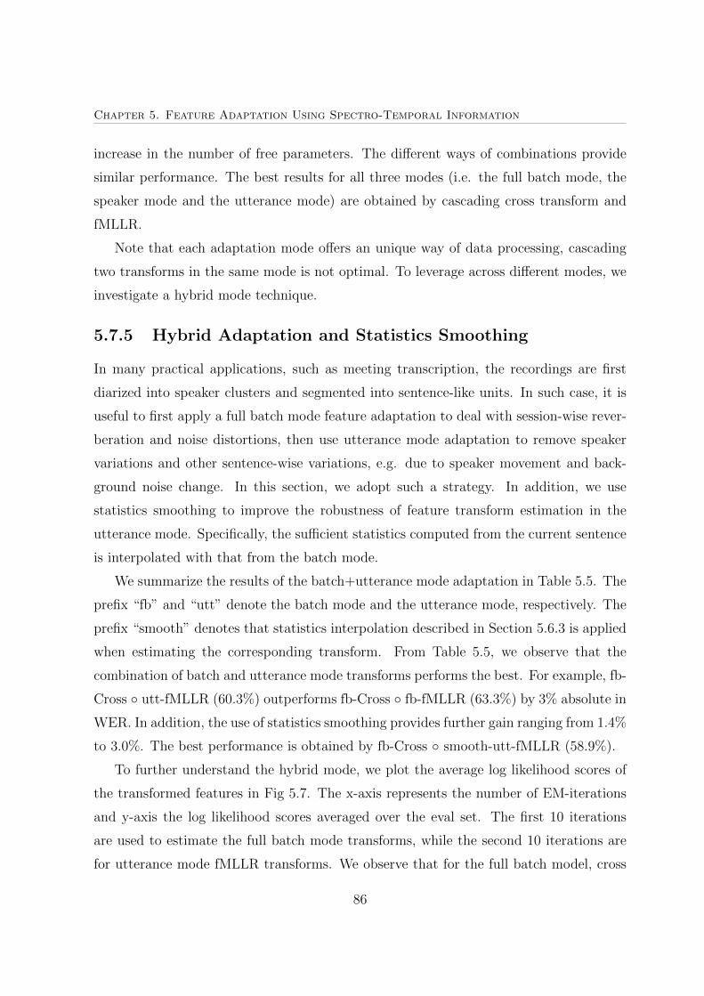
Chapter 5. Feature Adaptation Using Spectro-Temporal Information
increase in the number of free parameters. The different ways of combinations provide
similar performance. The best results for all three modes (i.e. the full batch mode, the
speaker mode and the utterance mode) are obtained by cascading cross transform and
fMLLR.
Note that each adaptation mode offers an unique way of data processing, cascading
two transforms in the same mode is not optimal. To leverage across different modes, we
investigate a hybrid mode technique.
5.7.5 Hybrid Adaptation and Statistics Smoothing
In many practical applications, such as meeting transcription, the recordings are first
diarized into speaker clusters and segmented into sentence-like units. In such case, it is
useful to first apply a full batch mode feature adaptation to deal with session-wise rever-
beration and noise distortions, then use utterance mode adaptation to remove speaker
variations and other sentence-wise variations, e.g. due to speaker movement and back-
ground noise change. In this section, we adopt such a strategy. In addition, we use
statistics smoothing to improve the robustness of feature transform estimation in the
utterance mode. Specifically, the sufficient statistics computed from the current sentence
is interpolated with that from the batch mode.
We summarize the results of the batch+utterance mode adaptation in Table 5.5. The
prefix “fb” and “utt” denote the batch mode and the utterance mode, respectively. The
prefix “smooth” denotes that statistics interpolation described in Section 5.6.3 is applied
when estimating the corresponding transform. From Table 5.5, we observe that the
combination of batch and utterance mode transforms performs the best. For example, fb-
Cross ◦ utt-fMLLR (60.3%) outperforms fb-Cross ◦ fb-fMLLR (63.3%) by 3% absolute in
WER. In addition, the use of statistics smoothing provides further gain ranging from 1.4%
to 3.0%. The best performance is obtained by fb-Cross ◦ smooth-utt-fMLLR (58.9%).
To further understand the hybrid mode, we plot the average log likelihood scores of
the transformed features in Fig 5.7. The x-axis represents the number of EM-iterations
and y-axis the log likelihood scores averaged over the eval set. The first 10 iterations
are used to estimate the full batch mode transforms, while the second 10 iterations are
for utterance mode fMLLR transforms. We observe that for the full batch model, cross
86
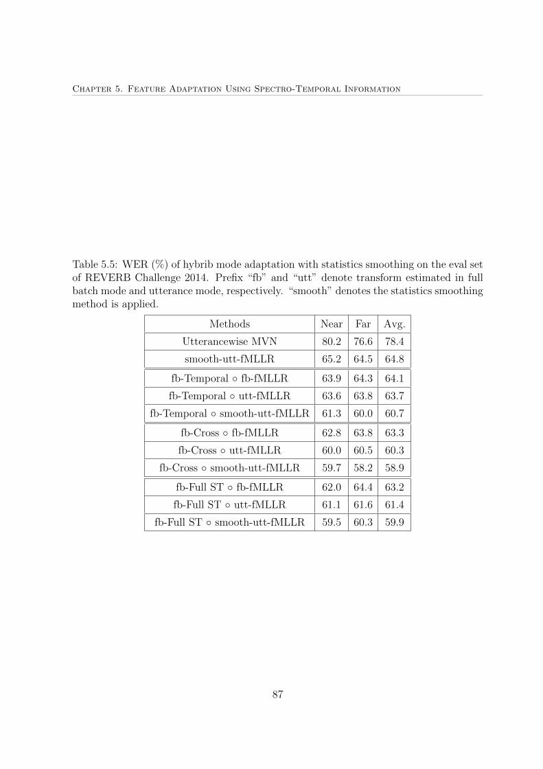
Chapter 5. Feature Adaptation Using Spectro-Temporal Information
Table 5.5: WER (%) of hybrib mode adaptation with statistics smoothing on the eval setof REVERB Challenge 2014. Prefix “fb” and “utt” denote transform estimated in fullbatch mode and utterance mode, respectively. “smooth” denotes the statistics smoothingmethod is applied.
Methods Near Far Avg.
Utterancewise MVN 80.2 76.6 78.4
smooth-utt-fMLLR 65.2 64.5 64.8
fb-Temporal ◦ fb-fMLLR 63.9 64.3 64.1
fb-Temporal ◦ utt-fMLLR 63.6 63.8 63.7
fb-Temporal ◦ smooth-utt-fMLLR 61.3 60.0 60.7
fb-Cross ◦ fb-fMLLR 62.8 63.8 63.3
fb-Cross ◦ utt-fMLLR 60.0 60.5 60.3
fb-Cross ◦ smooth-utt-fMLLR 59.7 58.2 58.9
fb-Full ST ◦ fb-fMLLR 62.0 64.4 63.2
fb-Full ST ◦ utt-fMLLR 61.1 61.6 61.4
fb-Full ST ◦ smooth-utt-fMLLR 59.5 60.3 59.9
87
Chapter 5. Feature Adaptation Using Spectro-Temporal Information
0 2 4 6 8 10 12 14 16 18 20−52
−51
−50
−49
−48
−47
−46
−45
−44
EM iterations
Average log−likelihood per frame
fb−cross
fb−cross + fb−fMLLR
fb−cross + smooth−utt−fMLLR
fb−full
fb−full + fb−fMLLR
fb−full + smooth−utt−fMLLR
fb−temporal
fb−temporal + fb−fMLLR
fb−temporal + smooth−utt−fMLLR
Figure 5.7: Log likelihood per frame averaged over the eval set. The first 10 EM-iterationsare used for full batch mode transform estimation, while the last 10 iterations are forfMLLR transforms estimated in either full batch mode or utterance mode with andwithout statistics smoothing.
transform achieves the highest likelihood, followed by full ST transform, and temporal
filter achieves the lowest likelihood as it does not use spectral information. Although the
full ST transform is supposed to be more detailed than the cross transform, it achieves
lower likelihood than the cross transform possibly due to the difficulty in optimizing the
objective function with a large amount of parameters. In the second stage (utterance
mode fMLLR), likelihood is improved significantly whenever the statistics smoothing is
applied. This shows that statistics smoothing is very important for reliable estimation of
the fMLLR transform. It is also worth pointing out that the final likelihood achieved by
each combination is highly correlated with their speech recognition performance achieved.
This show that the proposed minimum KL divergence cost function is suitable for feature
adaptation.
88
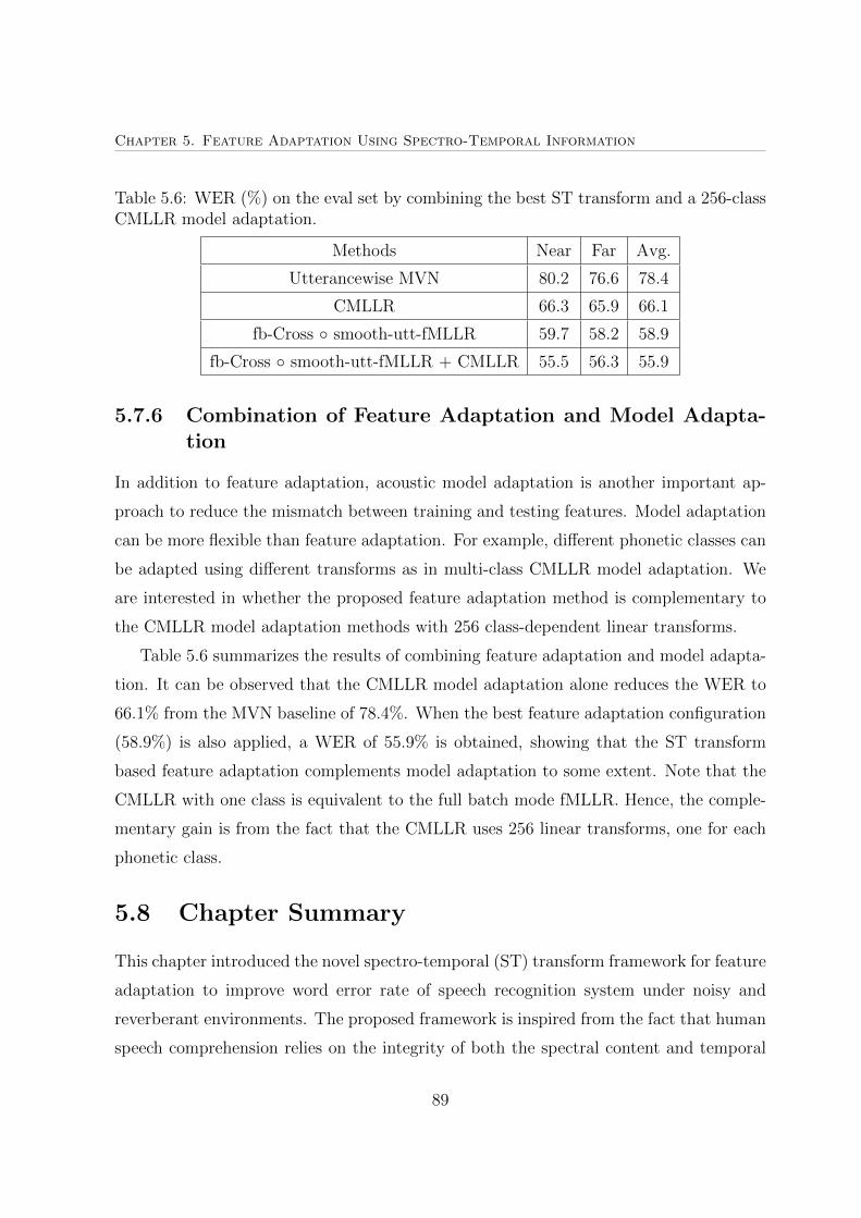
Chapter 5. Feature Adaptation Using Spectro-Temporal Information
Table 5.6: WER (%) on the eval set by combining the best ST transform and a 256-classCMLLR model adaptation.
Methods Near Far Avg.
Utterancewise MVN 80.2 76.6 78.4
CMLLR 66.3 65.9 66.1
fb-Cross ◦ smooth-utt-fMLLR 59.7 58.2 58.9
fb-Cross ◦ smooth-utt-fMLLR + CMLLR 55.5 56.3 55.9
5.7.6 Combination of Feature Adaptation and Model Adapta-tion
In addition to feature adaptation, acoustic model adaptation is another important ap-
proach to reduce the mismatch between training and testing features. Model adaptation
can be more flexible than feature adaptation. For example, different phonetic classes can
be adapted using different transforms as in multi-class CMLLR model adaptation. We
are interested in whether the proposed feature adaptation method is complementary to
the CMLLR model adaptation methods with 256 class-dependent linear transforms.
Table 5.6 summarizes the results of combining feature adaptation and model adapta-
tion. It can be observed that the CMLLR model adaptation alone reduces the WER to
66.1% from the MVN baseline of 78.4%. When the best feature adaptation configuration
(58.9%) is also applied, a WER of 55.9% is obtained, showing that the ST transform
based feature adaptation complements model adaptation to some extent. Note that the
CMLLR with one class is equivalent to the full batch mode fMLLR. Hence, the comple-
mentary gain is from the fact that the CMLLR uses 256 linear transforms, one for each
phonetic class.
5.8 Chapter Summary
This chapter introduced the novel spectro-temporal (ST) transform framework for feature
adaptation to improve word error rate of speech recognition system under noisy and
reverberant environments. The proposed framework is inspired from the fact that human
speech comprehension relies on the integrity of both the spectral content and temporal
89
Chapter 5. Feature Adaptation Using Spectro-Temporal Information
envelope of speech signal. The ST transform utilizes spectro-temporal information to
adapt run-time speech features to minimize the mismatch between run-time and training
data. The Kullback Leibler divergence based cost function is proposed to estimate the
transform parameters.
In practice, two implementations of the framework are conducted to cope with a lim-
itation issue of adaptation data. The first form is a cross transform which is a sparse
spectro-temporal transforms. The second form is a cascaded transform of temporal trans-
form and spectral transform. Both forms are effective and efficient to estimate ST trans-
form from limited adaptation data. In addition, the interpolation of statistics is also
applied to further improve the reliability of parameter estimates.
We conducted the experiments on REVERB Challenge 2014 benchmarking task where
the clean-condition trained acoustic models are tested on real reverberant and noisy
read speech recorded in meeting rooms. The experimental results confirmed that the
spectro-temporal transform outperforms a spectral or temporal only adaptation, with
cross transform achieving the best results. We have also explored alternative approaches
to ST transform implementation, such as cascaded transform and interpolation of statis-
tics. All experiments positively validated the idea of ST transform.
90
Chapter 6
Conclusions
This thesis has focussed on the topic of feature enhancement and adaptation for robust
speech recognition. The aim is to modify speech features in order to reduce mismatch
between training and testing speech data. The mismatch is challenging when the testing
environment is unknown and different from training environment. To overcome this,
three proposed feature-based methods were presented to improve the word accuracy of
speech recognition system. This chapter summarizes these methods and discusses some
possible future directions.
6.1 Contributions and Discussions
6.1.1 Noise Conditioning/Normalization Vector Taylor SeriesMethod
In chapter 3, the idea of noise conditioning/normalization to reduce non-stationary char-
acteristics of the additive noise in the speech is discussed. The proposed method can be
interpreted as a modification of spectral subtraction method or as an extension of VTS
model adaptation method. Instead of trying to completely remove additive noise such
as in [13], the method first normalizes the additive noise distribution towards a single
Gaussian model and then handles the remaining noise in the back-end phase by VTS
model compensation [11]. Our approach modifies the mismatch function and acoustic
model compensation of the VTS method to account for the remaining noise in the fea-
tures. The simulation results on Aurora-2 task showed 14.4% relative reduction of WER
over the VTS baseline.
91
Chapter 6. Conclusions
A drawback of the proposed method is that there is the lack of an integration of
non-stationary noise tracking into NN-VTS framework. The integration is very impor-
tant because the performance of NN-VTS is dependent on how accurately the noise is
estimated. Another limitation is that the quantification of the efficiency enhancement is
missing. Although the qualification is provided, it would be more complete if the quan-
tification is also investigated to be able to support the decision on the actual deployment.
6.1.2 PFC framework for LVCSR
The chapter 4 discusses the second proposed method which is an extension of particle filter
compensation (PFC) [35]. The proposed method aims to directly estimate clean speech
features. The idea of PFC is to utilize information from hidden Markov models (HMMs)
trained with clean speech to propagate the particles. Each particle represents a candidate
for a clean speech feature, and by weighting each candidate, the clean speech features
are predicted. The contribution of our work focused on how to obtain aligned state
sequence of HMMs that describe the underlying clean speech features being estimated
in noise. This task is challenging because the total number of triphone models involved
can be very large for sub-word based LVCSR . Our approach is to use separate sets of
HMMs for recognition and compensation. These two acoustic models are estimated from
a reference clean acoustic model using single pass retraining. Hence, the aligned state and
mixture sequence of noisy HMMs generated by a decoder can be used with clean HMMs
to propagate the particles which describe samples of clean speech features. In addition,
the models used for PFC can be simplified to a great extent and thus it facilitates the
estimation of the side information offered in the state and mixture sequences. When the
missing side information for PFC is available, a large word error reduction of 28.46%
from multi-condition training is observed for Aurora-4 database.
In this work, we found that the temporal structure of the PFC compensated static
features are seriously distorted. Hence, the proposed method needs to be improved to be
able to handle distortions of dynamic features. A suggestion is to enforce the correlation
between adjacent frames in a more explicit way. Another limitation is that in the current
PFC framework, we consider only the additive noise in background and use the simple
distortion model of noisy speech. A suggestion is to investigate the PFC with other
92
Chapter 6. Conclusions
distortion models presented in [1] to further improve the PFC framework. In real-life
application, there are usually both additive and convolutional noises and thus, extending
the current PFC method to take into account both types of noises is another potential
development.
6.1.3 Spectro-Temporal Transform
The third and last work of the thesis in chapter 5 discusses a spectro-temporal transform
for feature adaptation as well as a minimum KL divergence based cost function for
estimating the transform parameters. The new feature adaptation technique uses both
spectral and temporal information simultaneously, and hence is suitable to deal with both
spectral variability (e.g. speaker variation and noise distortions) and temporal variability
(e.g. reverberation). In addition, the link and relationship to existing feature adaptation
techniques is also discussed. In practice, to overcome limited training data problem, a
sparse generalized transform, called cross transform, is used to reduce the number of
parameters required.
Experiments were conducted on REVERB Challenge 2014 benchmarking task where
the clean and multi-condition trained acoustic models are tested on reverberant and noisy
meeting recordings. The experimental results confirmed that the spectro-temporal trans-
form outperforms a spectral or temporal only adaptation, with cross-transform achieving
the best results. Alternative approaches to ST transform implementation, such as cas-
caded transform and interpolation of statistics have also been explored. The experiments
positively validated the idea of ST transform.
There are still many aspects of feature adaptation worthy to be exploited in the future.
The cross transform is an empirically designed sparse transform. Another possibility is
to discover a sparse transform automatically by using sparse constraints such as L1 on
the parameters used in [84]. This could reveal which time-quefrency locations are most
useful for predicting the feature at the current location. To further improve reliability
of parameter estimation, subspace methods may be applied such as the one in [87] for
fMLLR. Another direction is to further increase the flexibility of the transform without
significantly increasing the number of free parameters. For example, we can introduce
nonlinear hidden nodes into the transform, similar to a multilayer perceptron. Nonlinear
93
Chapter 6. Conclusions
processing may be necessary as the distortion in cepstral domain are generally nonlinear.
Yet another direction is to model the training feature’s distribution better. GMM only
captures spectral and short term temporal information. Considering that the ST trans-
form uses both spectral and temporal information, it is more reasonable to use a reference
distribution that also captures these information of the training features. Finally, one
can also investigate the transform with existing state of the art DNN acoustic model to
study how a more powerful acoustic model than GMM affects on the proposed works.
6.2 Future Directions
Besides the development directions for each method have been discussed in previous
subsections, here are common future directions. In this work, three feature enhancement
methods for robust speech recognition have been proposed. However, it lacks comparisons
of these methods on a single corpus and using a single GMM/HMM reference system.
Conducting the comparative experiments will help us better to understand the proposed
methods. Another development approach is to integrate the proposed methods with the
state-of-the-art DNN-based recognition systems to further investigate the potential of
the proposed frameworks.
94
Bibliography
[1] X. D. Huang, A. Acero, and H. W. Hon, Spoken language processing: A guide to
theory, algorithm, and system development. Prentice-Hall, 2001.
[2] G. E. Hinton, L. Deng, D. Yu, G. E. Dahl, A. Mohamed, N. Jaitly, A. Senior,
V. Vanhoucke, P. Nguyen, T. Sainath, and B. Kingsbury, “Deep neural networks
for acoustic modeling in speech recognition: The shared views of four research
groups,” Signal Processing Magazine, IEEE, vol. 29, no. 6, pp. 82–97, 2012.
[3] J. L. Gauvain and C. H. Lee, “Maximum a posterirori estimation for multivariate
Gaussian mixture observations of Markov chains,” IEEE Trans. Speech and Audio
Processing, vol. 2, no. 2, pp. 291–298, Apr. 1994.
[4] M. J. F. Gales, “Maximum likelihood linear transformations for HMM-based speech
recognition,” Computer Speech and Language, vol. 12, pp. 75–98, 1998.
[5] C. J. Leggetter and P. C. Woodland, “Maximum likelihood linear regression for
speaker adaptation of continuous density hidden Markov models,” Computer Speech
and Language, vol. 9, no. 2, pp. 171–185, Apr. 1995.
[6] K. Shinoda and C.-H. Lee, “A structural Bayes approach to speaker adaptation,”
IEEE Trans. Speech Audio Process., vol. 9, no. 3, pp. 276–287, Mar 2001.
[7] O. Siohan, C. Chesta, and C.-H. Lee, “Joint maximum a posteriori adaptation of
transformation and HMM parameters,” IEEE Trans. Speech and Audio Processing,
vol. 9, no. 4, pp. 417–428, May 2001.
[8] O. Siohan, T. A. Myrvoll, and C.-H. Lee, “Structural maximum a posteriori linear
regression for fast HMM adaptation,” Computer Speech & Language, vol. 16, no. 1,
pp. 5 – 24, 2002.
95
BIBLIOGRAPHY
[9] M. Rahim and B. H. Juang, “Signal bias removal by maximum likelihood esti-
mation for robust telephone speech recognition,” IEEE Trans. Speech and Audio
Processing, vol. 4, no. 1, pp. 19–, Jan 1996.
[10] M. Gales and Y.-Q. Wang, “Model-based approaches to handling additive noise in
reverberant environments,” in Joint Workshop on Hands-free Speech Communica-
tion and Microphone Arrays (HSCMA), May 2011, pp. 121–126.
[11] J. Li, L. Deng, D. Yu, Y. Gong, and A. Acero, “A unified framework of HMM adap-
tation with joint compensation of additive and convolutive distortions,” Computer
Speech and Language, vol. 23, no. 3, pp. 389–405, Jul. 2009.
[12] A. Acero, L. Deng, T. Kristjansson, and J. Zhang, “HMM Adaptation Using Vector
Taylor Series for Noisy Speech Recognition,” in Proc. ICSLP ’00, Beijing, China,
Oct. 2000, pp. 869–872.
[13] S. F. Boll, “Suppression of acoustic noise in speech using spectral subtraction,”
IEEE Trans. Acoustics, Speech and Signal Processing, vol. 27, no. 2, pp. 113–120,
1979.
[14] J. S. Lim and A. V. Oppenheim, “Enhancement and bandwidth compression of
noisy speech,” Proc. IEEE, vol. 67, no. 12, pp. 1586–1604, Dec. 1979.
[15] Y. Ephraim and D. Malah, “Speech enhancement using a minimum mean square
error short time spectral amplitude estimator,” IEEE Trans. Acoustics, Speech and
Signal Processing, vol. 32, no. 6, pp. 1109–1121, Dec. 1984.
[16] ——, “Speech enhancement using a minimum mean square error Log-spectral am-
plitude estimator,” IEEE Trans. Acoustics, Speech and Signal Processing, vol. 33,
no. 2, pp. 443–445, Apr. 1985.
[17] B. W. Gillespie and L. Atlas, “Strategies for improving audible quality and speech
recognition accuracy of reverberant speech,” in Proc. ICASSP ’03, vol. 1, April
2003, pp. I–676–I–679 vol.1.
96
BIBLIOGRAPHY
[18] J. Hopgood and P. Rayner, “Blind single channel deconvolution using nonstationary
signal processing,” IEEE Trans. Speech and Audio Processing, vol. 11, no. 5, pp.
476–488, Sept 2003.
[19] T. Nakatani, T. Yoshioka, K. Kinoshita, M. Miyoshi, and B.-H. Juang, “Speech
dereverberation based on variance-normalized delayed linear prediction,” IEEE
Trans. Audio, Speech, and Language Processing, vol. 18, no. 7, pp. 1717–1731,
Sept 2010.
[20] H. Kameoka, T. Nakatani, and T. Yoshioka, “Robust speech dereverberation based
on non-negativity and sparse nature of speech spectrograms,” in Proc. ICASSP
’09, April 2009, pp. 45–48.
[21] J. Erkelens and R. Heusdens, “Correlation-based and model-based blind single-
channel late-reverberation suppression in noisy time-varying acoustical environ-
ments,” IEEE Trans. Audio, Speech, and Language Processing, vol. 18, no. 7, pp.
1746–1765, Sept 2010.
[22] K. Kumar, B. Raj, R. Singh, and R. Stern, “An iterative least-squares technique
for dereverberation,” in Proc. ICASSP ’11, May 2011, pp. 5488–5491.
[23] L. Deng, A. Acero, M. Plumpe, and X. D. Huang, “Large-vocabulary speech recog-
nition under adverse acoustic environment,” in Proc. ICSLP ’00, Beijing, China,
Oct. 2000, pp. 806–809.
[24] B. S. Atal, “Effectiveness of linear prediction characteristics of the speech wave for
automatic speaker identification and verification,” The Journal of the Acoustical
Society of America, vol. 55, no. 6, pp. 1304–1312, 1974. [Online]. Available:
http://scitation.aip.org/content/asa/journal/jasa/55/6/10.1121/1.1914702
[25] O. Viikki and K. Laurila, “Cepstral domain segmental feature vector normalization
for noise robust speech recognition,” Speech Communication, vol. 25, pp. 133–147,
1998.
97
BIBLIOGRAPHY
[26] S. Molau, F. Hilger, and H. Ney, “Feature space normalization in adverse acoustic
conditions,” in Proc. ICASSP ’03, vol. 1, Hong Kong, China, Apr. 2003, pp. 656–
659.
[27] H. Hermansky and N. Morgan, “RASTA processing of speech,” IEEE Trans. Speech
and Audio Processing, vol. 2, no. 4, pp. 578–589, 1994.
[28] H. Hermansky, N. Morgan, A. Bayya, and P. Kohn, “Compensation for the Effect of
the Communication Channel in Auditory-Like Analysis of Speech (RASTA-PLP),”
in European Conference on Speech Communication and Technology, 1991, pp. 1367–
1370.
[29] V. Digalakis, D. Rtischev, and L. G. Neumeyer, “Speaker adaptation using con-
strained estimation of Gaussian mixtures,” IEEE Trans. Speech and Audio Pro-
cessing, vol. 3, no. 5, pp. 357–366, 1995.
[30] C.-H. Lee and Q. Huo, “On adaptive decision rules and decision parameter adapta-
tion for automatic speech recognition,” Proc. IEEE, vol. 88, pp. 1241–1269, 2000.
[31] T. Yoshioka, A. Sehr, M. Delcroix, K. Kinoshita, R. Maas, T. Nakatani, and
W. Kellermann, “Making Machines Understand Us in Reverberant Rooms: Robust-
ness Against Reverberation for Automatic Speech Recognition,” Signal Processing
Magazine, IEEE, vol. 29, no. 6, pp. 114–126, Nov 2012.
[32] J. Li, L. Deng, Y. Gong, and R. Haeb-Umbach, “An Overview of Noise-Robust
Automatic Speech Recognition,” IEEE Trans. Audio, Speech, and Language Pro-
cessing, 2014.
[33] D. H. H. Nguyen, X. Xiao, E. S. Chng, and H. Li, “An analysis of vector taylor series
model compensation for non-stationary noise in speech recognition,” in ISCSLP,
Hong Kong, 2012.
[34] D. H. H. Nguyen, A. Mushtaq, X. Xiao, E. S. Chng, H. Li, and C.-H. Lee, “A
particle filter compensation approach to robust lvcsr,” in APSIPA ASC, Taiwan,
2013.
98
BIBLIOGRAPHY
[35] A. Mushtaq, Y. Tsao, and C.-H. Lee, “A particle filter feature compensation ap-
proach to robust speech recognition,” in Eleventh Annual Conference of the Inter-
national Speech Communication Association, 2010.
[36] D. H. H. Nguyen, X. Xiao, E. S. Chng, and H. Li, “Feature adaptation using linear
spectro-temporal transform for robust speech recognition,” IEEE/ACM Transac-
tions on Audio, Speech, and Language Processing, vol. PP, no. 99, pp. 1–1, 2016.
[37] D. H. H. Nguyen, X. Xiao, E. S. Chng, and H. Li, “Generalization of temporal
filter and linear transformation for robust speech recognition,” in Proc. ICASSP
’14, May 2014, pp. 1730–1734.
[38] S. Davis and P. Mermelstein, “Comparison of Parametric Representations for
Monosyllabic Word Recognition in Continuously Spoken Sentences,” IEEE Trans.
Acoustics, Speech and Signal Processing, vol. 28, pp. 357–366, 1980.
[39] G. von Bekesy, Experiments in Hearing. McGraw-Hill, 1960.
[40] H. Fletcher and W. Munson, “Loudness, its definition, measurement and calcu-
lation,” Journal of the Acoustical Society of America, vol. 5, no. 2, pp. 82–108,
1933.
[41] S. Furui, “Speaker independent isolated word recognizer using dynamic features of
speech spectrum,” IEEE Trans. Acoustics, Speech and Signal Processing, vol. 34,
no. 1, pp. 52–59, 1986.
[42] M. Gales and F. Flego, “Discriminative classifiers with generative kernels for noise
robust speech recognition,” CUED/TR605, University of Cambridge, Tech. Rep.,
2008.
[43] Z. Ghahramani, “An introduction to hidden markov models and bayesian
networks,” International Journal of Pattern Recognition and Artificial
Intelligence, vol. 15, no. 01, pp. 9–42, 2001. [Online]. Available:
http://www.worldscientific.com/doi/abs/10.1142/S0218001401000836
99
BIBLIOGRAPHY
[44] A. P. Dempster, N. M. Laird, and D. B. Rubin, “Maximum likelihood from incom-
plete data via the EM algorithm,” Journal of Royal Statistical Society, Series B
(Methodological), vol. 39, no. 1, pp. 1–38, 1977.
[45] T. N. Sainath, A. r. Mohamed, B. Kingsbury, and B. Ramabhadran, “Deep con-
volutional neural networks for lvcsr,” in 2013 IEEE International Conference on
Acoustics, Speech and Signal Processing, May 2013, pp. 8614–8618.
[46] T. Sercu, C. Puhrsch, B. Kingsbury, and Y. LeCun, “Very deep multilingual con-
volutional neural networks for lvcsr,” in 2016 IEEE International Conference on
Acoustics, Speech and Signal Processing (ICASSP), March 2016, pp. 4955–4959.
[47] X. Xiao, “Robust speech features and acoustic models for speech recognition,”
Ph.D. dissertation, School of Computer Engineering, Nanyang Technological Uni-
versity, Singapore, 2009.
[48] L. Deng, Front-End, Back-End, and Hybrid Techniques to Noise-Robust Speech
Recognition. Springer, 2011, ch. 4, pp. 67–99.
[49] A. de la Torre, A. M. Peinado, J. C. Segura, J. L. Perez-Cordoba, M. C. Benıtez,
and A. J. Rubio, “Histogram equalization of speech representation for robust
Speech Recognition,” IEEE Trans. Speech and Audio Processing, vol. 13, no. 3,
pp. 355–366, 2005.
[50] C.-P. Chen and J. A. Bilmes, “MVA Processing of Speech Features,” IEEE Trans.
Audio, Speech, and Language Processing, vol. 15, no. 1, pp. 257–270, 2007.
[51] P. J. Moreno, “Speech recognition in noisy environments,” Ph.D. dissertation, ECE,
Carnegie Mellon University, 1996.
[52] S.-H. Lin, B. Chen, and Y.-M. Yeh, “Exploring the Use of Speech Features and
Their Corresponding Distribution Characteristics for Robust Speech Recognition,”
IEEE Trans. Audio, Speech, and Language Processing, vol. 17, no. 1, pp. 84 –94,
jan. 2009.
100
BIBLIOGRAPHY
[53] X. Xiao, J. Li, H. Li, and E. S. Chng, “Maximum likelihood adaptation of histogram
equalization with constraint for robust speech recognition,” in Proc. ICASSP ’11,
Prague, Czech, May 2011, pp. 5480–5483.
[54] X. Xiao, E. S. Chng, and H. Li, “Normalization of the Speech Modulation Spec-
tra for Robust Speech Recognition,” IEEE Trans. Audio, Speech, and Language
Processing, vol. 16, no. 8, pp. 1662–1674, Nov. 2008.
[55] ——, “Joint Spectral and Temporal Normalization of Features for Robust Recog-
nition of Noisy and Reverberated Speech,” in Proc. ICASSP ’12, Kyoto, Japan,
Apr. 2012, pp. 4325–4328.
[56] ——, “Temporal filter design by minimum KL divergence criterion for robust speech
recognition,” in Proc. ICASSP ’13, Vancouver, Canada, May 2013.
[57] N. Moradi, B. Nasersharif, and A. Akbari, “Robust speech recognition using spec-
tral subtraction and temporal structure normalization,” in 2011 19th Iranian Con-
ference on Electrical Engineering, May 2011, pp. 1–4.
[58] S. S. Wang, Y. Tsao, and J. w. Hung, “Filtering on the temporal probability
sequence in histogram equalization for robust speech recognition,” in 2013 IEEE
International Conference on Acoustics, Speech and Signal Processing, May 2013,
pp. 7112–7116.
[59] C. A. Gordillo, J. R. B. de Marca, and A. Alcaim, “Median filtering the temporal
probability distribution in histogram mapping for robust continuous speech recog-
nition,” in 2016 24th European Signal Processing Conference (EUSIPCO), Aug
2016, pp. 1198–1201.
[60] C. Li and W.-J. Liu, “A novel multi-band spectral subtraction method based on
phase modification and magnitude compensation,” in Proc. IEEE Int Acoustics,
Speech and Signal Processing (ICASSP) Conf, 2011, pp. 4760–4763.
[61] P. Lockwood and J. Boudy, “Experiments with a nonlinear spec-
tral subtractor (nss), hidden markov models and the projection, for
101
BIBLIOGRAPHY
robust speech recognition in cars,” Speech Communication, vol. 11,
no. 2–3, pp. 215 – 228, 1992, eurospeech ’91. [Online]. Available:
//www.sciencedirect.com/science/article/pii/016763939290016Z
[62] C. He and G. Zweig, “Adaptive two-band spectral subtraction with multi-window
spectral estimation,” in 1999 IEEE International Conference on Acoustics, Speech,
and Signal Processing. Proceedings. ICASSP99 (Cat. No.99CH36258), vol. 2, Mar
1999, pp. 793–796 vol.2.
[63] B. L. Sim, Y. C. Tong, J. S. Chang, and C. T. Tan, “A parametric formulation of
the generalized spectral subtraction method,” IEEE Transactions on Speech and
Audio Processing, vol. 6, no. 4, pp. 328–337, Jul 1998.
[64] S. Kamath and P. Loizou, “A multi-band spectral subtraction method for enhancing
speech corrupted by colored noise,” in 2002 IEEE International Conference on
Acoustics, Speech, and Signal Processing, vol. 4, May 2002, pp. IV–4164–IV–4164.
[65] P. C. Loizou, Speech Enhancement: Theory and Practice, Second Edition. CRC
Press, February 25, 2013.
[66] L. Deng and X. Huang, “Challenges in adopting speech recognition,” Communica-
tions of the ACM, vol. 47, no. 1, pp. 69–75, 2004.
[67] L. Deng, A. Acero, M. Plumpe, and X. Huang, “Large-vocabulary speech recogni-
tion under adverse acoustic environments,” in Proc. Int. Conf. on Spoken Language
Processing, 2000.
[68] J. A. Arrowood and M. A. Clements, “Using Observation Uncertainty in HMM
Decoding,” in Seventh International Conference on Spoken Language Processing,
2002.
[69] H. Liao and M. Gales, “Issues with uncertainty decoding for
noise robust automatic speech recognition,” Speech Communication,
vol. 50, no. 4, pp. 265 – 277, 2008. [Online]. Available:
http://www.sciencedirect.com/science/article/pii/S0167639307001720
102
BIBLIOGRAPHY
[70] A. Krueger and R. Haeb-Umbach, Robust Speech Recognition of Uncertain or Miss-
ing Data. Springer Berlin Heidelberg, 2011, ch. A Model-Based Approach to Joint
Compensation of Noise and Reverberation for Speech Recognition, pp. 257–290.
[71] M. Wolfel, “Enhanced speech features by single-channel joint compensation of noise
and reverberation,” IEEE Trans. Audio, Speech, and Language Processing, vol. 17,
no. 2, pp. 312–323, Feb 2009.
[72] X. Xiao, S. Zhao, D. H. Ha Nguyen, X. Zhong, D. L. Jones, E. S. Chng, and H. Li,
“Speech dereverberation for enhancement and recognition using dynamic features
constrained deep neural networks and feature adaptation,” EURASIP Journal on
Advances in Signal Processing, vol. 2016, no. 1, p. 4, 2016. [Online]. Available:
http://dx.doi.org/10.1186/s13634-015-0300-4
[73] T. Ishii, H. Komiyama, T. Shinozaki, Y. Horiuchi, and S. Kuroiwa1, “Reverberant
speech recognition based on denoising autoencoder,” in Proc. INTERSPEECH ’13,
2013.
[74] X. Feng, Y. Zhang, and J. Glass, “Speech feature denoising and dereverberation
via deep autoencoders for noisy reverberant speech recognition,” in 2014 IEEE
International Conference on Acoustics, Speech and Signal Processing (ICASSP),
May 2014, pp. 1759–1763.
[75] Y. Ueda, L. Wang, A. Kai, X. Xiao, E. S. Chng, and H. Li, “Single-
channel dereverberation for distant-talking speech recognition by combining
denoising autoencoder and temporal structure normalization,” Journal of Signal
Processing Systems, vol. 82, no. 2, pp. 151–161, 2016. [Online]. Available:
http://dx.doi.org/10.1007/s11265-015-1007-3
[76] Q. Huo and C.-H. Lee, “On-line adaptive learning of the correlated continuous den-
sity hidden markov for speech recognition,” in IEEE Trans. Speech Audio Process.,
1998.
[77] K. Shinoda and C.-H. Lee, “Structural map speaker adaptation using hierarchical
priors,” in Proc. IEEE Workshop Automatic Speech Recognition and Understand-
ing, 1997, pp. 381–388.
103
BIBLIOGRAPHY
[78] M. Gales and P. Woodland, “Mean and Variance Adaptation within the MLLR
Framework,” Computer Speech & Language, vol. 10, pp. 249–264, 1996.
[79] C. Chesta, O. Siohan, and C.-H. Lee, “Maximum a posteriori linear regression for
hidden markov model adaptation,” in EUROSPEECH’99, 1999.
[80] S. Goronzy and R. Kompe, “A MAP-like weighting scheme for MLLR speaker
adaptation,” in EUROSPEECH’99, 1999.
[81] P. C. Woodland, “Speaker adaptation for continuous density HMMs: A review,”
in Proceedings of the ISCA, 2001, p. 119.
[82] O. Siohan, C. Chesta, and C.-H. Lee, “Hidden markov model adaptation using
maximum a posteriori linear regression,” in In Workshop on Robust Methods for
Speech Recognition in Adverse Conditions, 1999.
[83] J. Li, Y. Tsao, and C.-H. Lee, “Shrinkage model adaptation in automatic speech
recognition,” in INTERSPEECH, 2010.
[84] J. Li, M. Yuan, and C.-H. Lee, “LASSO Model Adaptation for Automatic Speech
Recognition,” in Workshop on Learning Architectures, Representations, and Op-
timization for Speech and Visual Information Processing, Bellevue, Washington,
USA, Jul. 2011.
[85] M. J. F. Gales, “Cluster adaptive training of hidden Markov models,” IEEE Trans.
Speech and Audio Processing, vol. 8, no. 4, pp. 417–428, 2000.
[86] R. Kuhn, P. Nguyen, J. C. Junqua, L. Goldwasser, N. Niedzielski, S. Fincke,
K. Field, and M. Contolini, “Eigenvoices for speaker adaptation,” in ICSLP, 1998,
p. 0303.
[87] K.-T. Chen, W.-W. Liau, H.-M. Wang, and L.-S. Lee, “Fast Speaker Adaptation
Using Eigenspace-Based Maximum Likelihood Linear Regression,” in International
Conference on Spoken Language Processing, 2000.
104
BIBLIOGRAPHY
[88] M. Gales, “Transformation smoothing for speaker and environmental adapta-
tion,” in 5th European Conference on Speech Communication and Technology (Eu-
rospeech), 1997.
[89] R. Kuhn, J.-C. Junqua, P. Nguyen, and N. Niedzielski, “Rapid speaker adaptation
in eigenvoice space,” IEEE Trans. Speech and Audio Processing, vol. 8, no. 6, pp.
695–707, Nov 2000.
[90] M. Gales, “Predictive model-based compensation schemes for robust speech
recognition,” Speech Communication, vol. 25, no. 1-3, pp. 49 – 74, 1998. [Online].
Available: http://www.sciencedirect.com/science/article/pii/S0167639398000296
[91] A. Acero, “Acoustical and environmental robustness in automatic speech recogni-
tion,” Ph.D. dissertation, ECE, Carnegie Mellon University, 1990.
[92] M. J. F. Gales, Robust Speech Recognition of Uncertain or Missing Data Theory
and Applications. Springer-Verlag Berlin Heidelberg, 2011, ch. Model-Based Ap-
proaches to Handling Uncertainty, pp. 101–125.
[93] ——, “Model-based techniques for noise robust speech recognition,” Ph.D. disser-
tation, Gonville and Caius College, University of Cambridge, 1995.
[94] M. Abramowitz and I. A. Stegun, Eds., Handbook of Mathematical Functions: with
Formulas, Graphs, and Mathematical Tables. Dover Publications, 1972.
[95] H. Liao, “Uncertainty decoding for noise robust speech recognition,” Ph.D. disser-
tation, University of Cambr idge, 2007.
[96] J. Li, L. Deng, D. Yu, Y. Gong, and A. Acero, “High-performance HMM adaptation
with joint compensation of additive and convolutive distortions via vector taylor
series,” in Proc. ASRU ’07, Kyoto, Japan, Dec. 2007, pp. 65–70.
[97] D. Pearce and H.-G. Hirsch, “The AURORA experimental framework for the per-
formance evaluation of speech recogntion systems under noisy conditions,” in Proc.
ICSLP ’00, vol. 4, Beijing, China, Oct. 2000, pp. 29–32.
105
BIBLIOGRAPHY
[98] N. J. Gordon, D. J. Salmond, and A. F. M. Smith, “Novel approach to
nonlinear/non-gaussian bayesian state estimation,” IEE Proceedings F - Radar and
Signal Processing, vol. 140, no. 2, pp. 107–113, April 1993.
[99] R. Brown and P. Hwang, “Introduction to random signals and applied kalman
filtering. 1997,” NY John Wiley and Sons.
[100] S. Haykin, Adaptive Filter Theory. Prentice-Hall, 2002.
[101] R. Singh and B. Raj, “Tracking noise via dynamical systems with a contin-
uum of states,” in Acoustics, Speech, and Signal Processing, 2003. Proceed-
ings.(ICASSP’03). 2003 IEEE International Conference on, vol. 1. IEEE, 2003,
pp. I–396.
[102] B. Raj, R. Singh, and R. Stern, “On tracking noise with linear dynamical
system models,” in Acoustics, Speech, and Signal Processing, 2004. Proceed-
ings.(ICASSP’04). IEEE International Conference on, vol. 1. IEEE, 2004, pp.
I–965.
[103] M. Fujimoto and S. Nakamura, “Sequential non-stationary noise tracking using
particle filtering with switching dynamical system,” in Acoustics, Speech and Signal
Processing, 2006. ICASSP 2006 Proceedings. 2006 IEEE International Conference
on, vol. 1. IEEE, 2006, pp. I–I.
[104] A. Mushtaq and C.-H. Lee, “An integrated approach to feature compensation com-
bining particle filters and hidden markov model for robust speech recognition,” in
Acoustics, Speech and Signal Processing, 2012. ICASSP 2012 Proceedings. 2012
IEEE International Conference on, vol. 1. IEEE, 2012, pp. I–I.
[105] S. Young et al., The HTK book, 3rd ed. Cambridge university engineering depart-
ment, 2006.
[106] M. Arulampalam, S. Maskell, N. Gordon, and T. Clapp, “A tutorial on particle fil-
ters for online nonlinear/non-gaussian bayesian tracking,” Signal Processing, IEEE
Transactions on, vol. 50, no. 2, pp. 174–188, 2002.
106
BIBLIOGRAPHY
[107] G. Saon, G. Zweig, and M. Padmanabhan, “Linear feature space projections for
speaker adaptation,” in Proc. ICASSP ’01, vol. 1, 2001, pp. 325–328 vol.1.
[108] A. Sankar and C.-H. Lee, “A maximum-likelihood approach to stochastic matching
for robust speech recognition,” IEEE Trans. Speech and Audio Processing, vol. 4,
no. 3, pp. 190–202, May 1996.
[109] E. Ahissar, S. Nagarajan, M. Ahissar, A. Protopapas, H. Mahncke, and
M. M. Merzenich, “Speech comprehension is correlated with temporal response
patterns recorded from auditory cortex,” Proceedings of the National Academy
of Sciences, vol. 98, no. 23, pp. 13 367–13 372, 2001. [Online]. Available:
http://www.pnas.org/content/98/23/13367.abstract
[110] F. E. Theunissen, K. Sen, and A. J. Doupe, “Spectral-temporal receptive fields of
nonlinear auditory neurons obtained using natural sounds,” The Journal of Neu-
roscience, vol. 20, no. 6, pp. 2315–2331, 2000.
[111] T. Chi, P. Ru, and S. A. Shamma, “Multiresolution spectrotemporal analysis of
complex sounds,” The Journal of the Acoustical Society of America, vol. 118, no. 2,
pp. 887–906, 2005.
[112] M. Kleinschmidt, D. Gelbart et al., “Improving word accuracy with gabor feature
extraction.” in INTERSPEECH, 2002.
[113] S. Ganapathy, S. H. Mallidi, and H. Hermansky, “Robust feature extraction using
modulation filtering of autoregressive models,” IEEE/ACM Transactions on Audio,
Speech and Language Processing (TASLP), vol. 22, no. 8, pp. 1285–1295, 2014.
[114] A. Papoulis and S. U. Pillai, Probability, random variables and stochastic processes,
4th ed. McGraw Hill, 2002.
[115] G. Saon, G. Zweig, and M. Padmanabhan, “Linear feature space projections for
speaker adaptation,” in Acoustics, Speech, and Signal Processing, 2001. Proceed-
ings.(ICASSP’01). 2001 IEEE International Conference on, vol. 1. IEEE, 2001,
pp. 325–328.
107
BIBLIOGRAPHY
[116] N. Kumar and A. G. Andreou, “Heteroscedastic discriminant analysis
and reduced rank HMMs for improved speech recognition,” Speech Com-
munication, vol. 26, no. 4, pp. 283 – 297, 1998. [Online]. Available:
http://www.sciencedirect.com/science/article/pii/S0167639398000612
[117] G. Saon, G. Zweig, B. Kingsbury, L. Mangu, and U. V. Chaudhari, “An archi-
tecture for rapid decoding of large vocabulary conversational speech,” in Proc.
INTERSPEECH ’03, Geneva, Switzerland, Sep. 2003.
[118] S. Kullback and R. A. Leibler, “On information and sufficiency,” Ann.
Math. Statist., vol. 22, no. 1, pp. 79–86, 03 1951. [Online]. Available:
http://dx.doi.org/10.1214/aoms/1177729694
[119] C. Bishop, Pattern Recognition and Machine Learning, 1st ed. Springer, 2006.
[120] D. C. Liu and J. Nocedal, “On the limited memory BFGS method for large scale
optimization,” Math. Program., vol. 45, no. 3, pp. 503–528, Dec. 1989.
[121] X. Lei, J. Hamaker, and X. He, “Robust Feature Space Adaptation For Telephony
Speech Recognition.” in Proc. INTERSPEECH ’06, 2006.
[122] S. Yoshizawa, A. Baba, K. Matsunami, Y. Mera, M. Yamada, and K. Shikano,
“Unsupervised speaker adaptation based on sufficient hmm statistics of selected
speakers,” in Proc. ICASSP ’01, vol. 1, 2001, pp. 341–344 vol.1.
[123] Y. Li, H. Erdogan, Y. Gao, and E. Marcheret, “Incremental On-Line Feature Space
MLLR Adaptation for Telephony Speech Recognition,” in Proc. ICSLP ’02, Den-
ver, USA, Sep. 2002, pp. 1417–1420.
[124] Z. ZajAc, L. Machlica, and L. MA14ller, “Initialization of fmllr with sufficient statis-
tics from similar speakers,” in Text, Speech and Dialogue, ser. Lecture Notes in
Computer Science, I. Habernal and V. MatouA¡ek, Eds. Springer Berlin Heidel-
berg, 2011, vol. 6836, pp. 187–194.
[125] O. Viikki, D. Bye, and K. Laurila, “A recursive feature vector normalization ap-
proach for robust speech recognition in noise,” in Proc. ICASSP ’98, Seattle, WA,
May 1998, pp. 733–736.
108
BIBLIOGRAPHY
[126] K. Kinoshita, M. Delcroix, T. Yoshioka, T. Nakatani, E. Habets, R. Haeb-Umbach,
V. Leutnant, A. Sehr, W. Kellermann, R. Maas, S. Gannot, and B. Raj, “The
REVERB Challenge: A Common Evaluation Framework for Dereverberation and
Recognition of Reverberant Speech,” in Proceedings of the IEEE Workshop on
Applications of Signal Processing to Audio and Acoustics (WASPAA-13), 2013.
[127] T. Robinson, J. Fransen, D. Pye, J. Foote, and S. Renals, “WSJCAM0: a British
English speech corpus for large vocabulary continuous speech recognition,” in Proc.
ICASSP ’95, 1995, pp. 81–84.
[128] M. Lincoln, I. McCowan, J. Vepa, and H. K. Maganti, “The multi-channel Wall
Street Journal audio visual corpus (MC-WSJ-AV): specification and initial experi-
ments,” in Proc. ASRU ’05, 2005, pp. 357–362.
109