Feeling the blues

Moral hazard and debt dilution in Eurobonds before 1914

Rui Pedro Esteves†

Ali Coşkun Tunçer ‡

November 2013

Abstract

Debt mutualisation through Eurobonds has been proposed as a solution to the

Euro crisis. Although this proposal has found some support, it also attracted

strong criticisms as it risks raising the spreads for strong countries, diluting legacy

debt and promoting moral hazard by weak countries. Because Eurobonds are a

new addition to the policy toolkit, there are many untested hypotheses in the

literature about the counterfactual behaviour of markets and sovereigns. This

paper offers some tests of the issues by drawing from the closest historical

parallel–five guaranteed bonds issued in Europe between 1833 and 1913. The

empirical evidence suggests that contemporary concerns about fiscal transfers

and debt dilution may be overblown, whilst creditors’ moral hazard may be as

much of a problem as debtors’.

JEL Codes: F34, H63, H77, N24, N44

Keywords: Eurobonds, Debt Mutualisation, Debt Dilution, Moral Hazard, Pre-1913

† University of Oxford, Economics Department, Manor Road, Oxford OX13UQ; rui.esteves@economics.ox.ac.uk

‡ University College London, History Department, Gower Street, London WC1E6BT; a.tuncer@ucl.ac.uk

1

1. Introduction

The recent debate on European sovereign debt crisis has attracted different proposals in policy fora.

These involve mostly unpopular solutions ranging from structural reforms, stronger federalism and

higher inflation targets to debt mutualisation (Eurobonds). Having appeared under different labels

and guises, the Eurobonds proposal, in essence, recommends the governments of the EU countries

to pool all or a certain portion of their debts together. This would presumably reduce borrowing

costs for sovereigns and induce much needed stability to the European sovereign debt market.

Although this proposal has found some support, it also attracted strong criticisms for its potential

negative impacts, particularly the risks of moral hazard and the dilution of current outstanding debt.

Compared to other tried solutions for fiscal crises, such as debt restructuring or default, inflation

and devaluation, possibly combined with liquidity assistance and stabilization plans from

multilaterals, there is precious little evidence on the potential effectiveness of the Eurobonds

proposal. The bailout and recapitalisation programmes organised since 2010 offer some suggestive

evidence of how Eurobonds could fare in the market, particularly after the reduction in mid-2011 of

the interest paid by programme countries to close to the effective cost of funding of multilaterals.

However, it is questionable whether the relatively short experience with these loans is a good

estimate of the consequences of debt mutualisation for the future of European financial stability.

The debate has therefore been mainly informed by untested hypotheses about the behaviour of

financial markets and sovereigns after the issue of Eurobonds.

This paper aims at contributing to this debate by drawing parallels with the guaranteed bonds

issued by several countries before 1914. Somewhat ironically, these operations started with a Greek

loan in 1832, which can arguably be considered the first Eurobond in history. The bonds we study

here were issued with the guaranty of another sovereign, usually a combination of the great powers

of the time (Britain, France, Germany and Russia) and were perceived by the market as instances of

debt mutualisation. Perhaps because of the risks involved, these loans were raised very sparsely and

often only after overcoming considerable political opposition within the guarantor countries

themselves. After the first Greek loan, there were only four other guaranteed loans issued in our

period of study – for Turkey in 1855, Egypt in 1885, China in 1895, and Greece again in 1898.

In this paper, we use the long historical record of these loans to address two main questions –

how the introduction of guaranteed bonds impacted existing creditors and how guaranteed debt

was priced by financial markets relative to the other financial liabilities of the nations involved.

The first question focuses on the short-time horizon around the announcement and flotation of

guaranteed bonds. By using an original dataset of daily secondary market prices, we investigate the

direct dilution of previous claims on the sovereign, which depended on the relative shares of ‘blue’

(guaranteed) and ‘red’ (non-guaranteed) bonds, seniority dispositions, possible write-downs of

existing debts, liquidity of the new issues, and, when included, the benefits from foreign-imposed

conditionality.

The second question has to be addressed over longer time horizons. In this part of the paper we

quantify the evolution of the spreads of guaranteed bonds relative to other non-guaranteed

domestic bonds, and investigate the relation between the yields of guaranteed bonds, their non-

guaranteed cousins, and their avuncular guarantors. These spreads are informative of the structural

2

impact of these debt relief operations on the fiscal positions of the recipient nations and should help

with addressing the contemporary criticisms about debtor’s moral hazard from the issue of

Eurobonds.

Our paper also relates to the literature on non-sovereign borrowing and foreign financial

intervention in the pre-1914 period. Two of the countries under study here (China and Egypt) were

under a status of informal colonial dependency from outside Powers. Nevertheless, we will show

that guaranteed bonds of these countries were perceived differently in the market from other

colonial issues, in that they were not priced entirely on the fiat of the colonial power. Colonial issues

were more than guaranteed by the coloniser, as the latter reserved complete control over colonial

finances (Accominotti et al. 2010). A different category of bonds were those issued under the

financial (and sometimes political) control of foreign creditors, where the latter controlled the

domestic sources of revenue set aside to service the foreign debt (Mitchener and Weidenmier

2010). Two of the case studies in this paper (Egypt in 1885 and Greece in 1898) fall in this category,

but differ from it in the sense that foreign creditors not only took control of local finances but

provided additional support through guaranteed loans. Foreign control certainly increased the

credibility of each sovereign, however it did not guarantee any repayments as in guaranteed bonds.

Moreover, there was not a perfect overlap between the list of guarantors and the Powers with a say

in financial control. For instance, the Greek 1898 bond was guaranteed by France, Britain and Russia

and floated simultaneously with the imposition of external control, where not only the guaranteeing

powers were represented but also Austria, Germany, and Italy.

The next section describes and compares the current proposals for the issuance of Eurobonds

with the corresponding debate in the nineteenth century, emphasising the similarities between the

two. Section 3 provides a simple framework to think about the relation between debt dilution and

fiscal discipline in terms of their impact on sovereign spreads. Section 4 contains the empirical

analysis split into two parts. In a first part we use structural breakpoint methods to identify the

short-run impact of the introduction of guaranteed bonds on the previous debt stock. In the second

part we investigate the pricing relations between guaranteed and non-guaranteed bonds with the

help of factor analysis and dynamic panel VARs. A conclusion follows.

2. The policy debate

2.1 Today: Eurobonds

Although the idea of increased coordination of public debt in Europe had been floated around the

introduction of the Euro, it did not get much mileage at the time. The report of the Giovannini Group

(2000) was mostly sceptical about the purported benefits. The proposal re-emerged in the very

different context of the Euro crisis. Whereas the Giovannini group had concentrated on the long-

term or steady-state costs and benefits, the new debate focused more on stabilising the European

market for sovereign debt and the financial system (Brunnermeier et al. 2011, Angeloni and Wolff

2012).

Between September 2008 and September 2011 a half-dozen alternative plans to implement

some version of Eurobonds emerged in the literature from academics, trade associations and official

3

organisations. All aim to fulfil a combination of four objectives: manage the current crisis, reinforce

financial stability and facilitate the transmission of monetary policy in the Euro area, improve market

efficiency, and enhance the international role of the Euro. Despite the commonality of objectives the

various plans diverge on several levels, especially on the questions of coverage and guaranties.

The majority of plans recommend that Eurobonds cover only partially the funding requirements

of member countries. The exceptions are Dübel (2011) and Beck, Wagner and Uhlig (2011), who

favour the issue of ‘synthetic Eurobonds’ to swap for all the sovereign debt stock in banking

portfolios (including the ECB). Similarly, Brunnermeier et al. (2011) propose to swap the entirety of

existing debt into two tranches of joint bonds. However, only the first or senior tranche (ESBies)

would be virtually safe from default, whereas the second tranche of junior bonds (EJBs) would take

any losses first. A related question is whether Eurobonds should be issued only in the primary

market or also to swap for existing debt. In the first case, only the marginal cost of funding would be

affected for participating countries, whereas in the second the average cost would also fall if yields

on Eurobonds were lower, as expected.

The most salient proposals for the partial issue of Eurobonds are the ‘blue/red bonds’ of Delpla

and von Weizsäcker (2010) and the ‘safe bonds’ of Bofinger et al. (2011). The two have diametrically

opposed approaches. Blue bonds, jointly issued, should be capped at a fraction of GDP (possibly 60%

as in the Maastricht criteria), whereas any excess debt would remain the responsibility of individual

countries that continued to issue their own ‘red’ bonds. Bofinger et al. (2011) only mutualise the

excess debt above 60% of GDP, though in the context of a redemption plan to extinguish it over the

medium-term.

The second main choice relates to the attachment of guaranties to the common bonds. Some

proposals require joint responsibility for common bonds, despite its likely violation of the no-bailout

clause of the European treaties (Delpla and von Wiezsäcker 2010, Jones 2010, Barclays Capital 2011,

Favero and Missale 2011). Precisely because of this, other authors consider that several guaranties,

where each country is only responsible for the service of its share of the common bonds, would be

enough (De Grauwe and Moesen 2009, Brunnermeier et al. 2011). Some authors provision for

further guaranties in the form of seniority clauses over pre-existing debt, or credit enhancements,

such as shock-absorbing collateral (cash or gold reserves) – particularly with a view to ensure that

the new Eurobonds would be rated AAA by credit ratings agencies.1

Given the breadth of these proposals it is not surprising that the expected impacts of their

undertaking also vary considerably, namely when compared with the four objectives listed at the

beginning of this section. The most obvious beneficiaries are the ‘weak countries’ currently facing a

widening of spreads.2 Either through pooling, diversification, seniority or credit enhancements, the

new Eurobonds are expected to pay lower yields than most national debts, thereby allowing

countries a cheaper access to funds. This is especially important during financial crises, when

markets can no longer price risk efficiently and may spread financial trouble through contagion, a

problem to which the Delors (1989) report already alerted. Furthermore, the yields effectively paid

by participating countries could be adjusted relative to the cost of funding of the Eurobonds-issuing

1 Practically all proposals favour seniority, with the exception of Dübel (2011) and Favero and Missale (2011).

2 Nevertheless, all proposals exclude the programme countries, currently undergoing bailout arrangements

with the ‘troika’ (ECB, EC, and IMF), at least until these programmes are completed.

4

agency so as to incentivise fiscal consolidation (Bonstra 2010, Dübel 2011, Muellbauer 2011 and

2013, European Commission 2011). Countries pursuing ‘bad fiscal policies’ would face an increasing

schedule of funding costs, whilst others would be compensated for their fiscal efforts. This would

also help preventing the build-up of unsustainable debt problems, similar to what happened after

the introduction of the Euro when markets were not able to screen sovereign risk adequately.

‘Strong countries’ with normal access to wholesale markets would also benefit indirectly, and

perhaps even directly, from the creation of Eurobonds. The main indirect benefits are financial

stability and greater efficiency in monetary policy transmission within the Eurozone, once the home

bias in banking portfolios of sovereign debt is replaced with a the issue of a safe(r) asset on which

the whole financial system can base itself. More pointedly, Jones (2010), Brunnermeier et al. (2011)

and Varoufakis and Holland (2011) consider that Eurobonds would be an efficient way of recycling

surpluses within the Eurozone without destabilising current accounts, and allowing countries such as

Germany to continue pursuing their export-led growth. Direct benefits would come in the way of

greater liquidity of the joint bonds, as well as a greater international role for the Euro. The two are

related in the sense that some authors consider that the role of the Euro as reserve currency is

hampered by the fragmented issue of sovereign bonds in the Eurozone that does not allow for the

creation of a benchmark asset comparable to the US T bonds.3 Interestingly, although mentioned by

all proposals, the estimates of gains are very limited, ranging from 30 to 70 basis points in the more

optimistic assessments to close to nothing in the more conservative estimates of the European

Commission’s (2011) Green Paper and Favero and Missale (2011).4

This raises the question of how to motivate the participation of stronger countries in the

Eurobonds issuance, as the liquidity gains might not compensate for the increase in funding costs

from pooling risk with weaker nations. Several proposals address this issue by including explicit

mechanisms to redistribute a share of the gains to the stronger nations, such that all participants

benefit from the system (De Grauwe and Moesen 2009, Boonstra 2010, NATIXIS 2011). Although

theoretically and algebraically conceivable, these redistribution rules raise practical implementation

questions. Two of the most important are the time consistency of these rules and their consistency

with fiscal stabilisation in the Eurozone.

Moreover, there is also considerable scepticism in the literature about the net advantages of the

Eurobonds proposals, not to mention about the political feasibility of the idea currently in Europe.

Starting with tranching and seniority, several studies point out that a Modigliani-Miller effect may

apply with negative consequences for nations’ ability to roll over their stocks of ‘red debt.’ By virtue

of the issue of Eurobonds nothing is changed in the underlying fiscal position of individual countries,

consequently if a tranche of ‘blue’, ‘safe’, or ‘synthetic’ bonds is carved out of their debt stocks with

seniority and enhanced guaranties, the remaining debt stock will have to bear the brunt of greater

illiquidity and risk premia (Kopf 2011, Brunnermeier et al. 2011, Claessens et al. 2012). The obvious

way of avoiding this would be to swap the full stock of ‘legacy debt’ with Eurobonds, but that raises

equally obvious concerns about moral hazard. The counterargument to this is that the maintenance

of stocks of national debt is a way of distinguishing between liquidity and risk premia, the former

3 On top of the liquidity discount, T bonds are also sought after as ‘safe haven’ which gives them an extra yield

advantage over German Bunds. 4 However, the latter estimates may be contaminated by the fact that the German Bunds and the bonds of

other AAA Euro-members have already benefited from a ‘safe haven’ status since 2009.

5

reduced through Eurobonds while the latter would continue to be priced by the markets. An

intermediate solution requires a careful calibration of the relative size of multilateral and national

bonds. The share of ‘blue bonds’ has to be large enough to improve fiscal sustainability ratios, but

small enough to allow countries to maintain market access at affordable interest rates (Gros 2010).

Moral hazard concerns loom large among the critics of Eurobonds, particularly since the recent

experience of the SGP implies that even ex-ante firm rules are time inconsistent in the context of a

financial crisis, and all the more because of the high level of cross-border financial integration in the

EU (see Issing 2009, Gros 2011 and Favero and Missale 2011, among many). Kopf refers to this as

“an illusion of seniority that cannot be enforced in times of crisis. In the end, member countries that

wish to remain current on their own obligations may end up having to pay for Portuguese, Greek or

Irish sovereign debt.”5

This incentive problem might completely negate the expected liquidity gains of a common

Eurobond benchmark issue. In a survey conducted in 2008, primary market dealers and credit rating

agencies were uniformly averse to joint guaranties of Eurobonds, as well as to insurance

mechanisms that pool risk between strong and weak nations (EPDA 2008). The latter were seen a

new incarnation of the structured products which were behind the financial crisis of 2008. However,

Eurobonds with several guaranties are not immune from problems either, as credit rating agencies

such as Standard & Poor’s have warned that their rating may not be above (as desired), or at least at

the level of the average ratings of the participating nations, but in fact below, and possibly as lower

as the lowest individual rating. This has a counterpart in the convexity of risk premia, which may rise

more than proportionally than underlying risk factors, such that the average risk premium of a

portfolio of bonds may be higher than the premium charged to an individual country with the same

average risk. We will return to these considerations in the next section.

2.2 Back then: guaranteed bonds

Although the discussion over Eurobonds has taken place with very limited historical reference, the

sovereign debt market before 1914 had several striking parallels to the proposals listed above. The

emergence of an international bond market and the boom in foreign securities during the 1820s

marked an important milestone in the evolution of sovereign debt contracts. This was also the case

after the debt crises of the 1870s, which led to new ways of dealing with defaults.6 One common

way of ensuring repayment of government bonds was to link each issue to a form of security. These

security clauses served the interest of creditors, as they safeguarded the interest and capital

payments of a loan in the absence of a multilateral enforcement mechanism. Similarly, borrower

governments had positive incentives to provide such securities given that their quality and extent

could be an important determinant of the cost of credit.

From the 1820s to 1914 there was considerable variation in the methods for securing sovereign

bonds These methods involved pledging the real estate of sovereigns as collateral, using tangible

assets or assigning part of or the entire state revenues of the debtor as a pledge.7 These revenues

5 Kopf (2011: 9).

6 Wynne (1951), Suter (1992), Neal (1998), Neal and Davis (2006), Flandreau and Flores (2009).

7 Borchard (1951), Cannon (1972), Hoyle (1986).

6

could be from any source. State monopolies, custom and railway revenues, tithes and even annuities

received from tributary states could be used to secure new loans. For instance, the Greek

independence loans of 1824 and 1825 were both secured by “all revenues and the whole national

property of Greece”.8 Although assigning government revenues looked like an attractive solution to

increase the credibility of a sovereign, in fact it could reduce the future borrowing capacity of a

country if the entire or part of the state revenues had already been pledged for the service of

previous loans. Another example of this was the Chinese guaranteed loan of 1895 secured by the

Imperial Maritime Customs, which had already been pledged for previous debt issues. This fact did

not escape contemporary observers:

“Pledging the maritime customs the Chinese government is alienating a source of revenue upon

which it will probably find it very difficult to get on without… The broad fact is, that the one

really good security which China has to offer has already been charged pretty heavily, and the

idea which seems to prevail at present that she may safely be trusted to almost any extent is

utterly fallacious.”9

These overlaps in securities attached to each bond could lead to legal problems in the case of a

default or debt readjustment especially if seniority between bonds was not clearly assigned.

Sovereign immunity also raised questions about the enforcement of this security–except if creditors

had direct control over the specific assets or revenues pledged. In the second half of the nineteenth

century these enforcement problems encouraged bondholders to establish revenue administrations

in Tunisia, Egypt, the Ottoman Empire, Serbia and Greece, among others. Through them creditors

were granted direct access to the revenues assigned for the service of the debt. Although these

revenue administrations had a positive impact on the credibility of debtor countries and increased

their future borrowing capacity, their success relied on the cooperation of debtor governments, thus

they did not guarantee any future repayments for creditors.10

One of the strongest ways of securing bonds before 1914 was through the issue of guaranteed

loans, which relied on the credit of other states rather than on the debtor’s own. In this period we

identified five guaranteed bonds, as described in Table 1. The Table summarises the main features of

each bond, namely, the guarantor states and their average cost of funding, the nature of each

guaranty, the nominal value, interest rate and issue price of each bond, and the previous debt stock

of the borrower country.

Table 1 here

There are three main characteristics of these bonds. First, the relationship between guarantors and

debtors was usually determined by political considerations of the guarantor states –mostly one or a

combination of the great powers of the time, i.e. Britain, France, and Russia. The first guaranteed

bond, issued in support of Greece after its independence from the Ottoman Empire in 1833 was the

first example of the involvement of the great powers into such an arrangement. Similarly in 1855,

the French and British governments agreed to guarantee a loan in order to support the Ottoman

8 Wynne (1951: 285).

9 “Chinese Borrowing” The Economist (London, England), Saturday, July 13, 1895; pg. 907

10 On this see Deville (1912), Hyde (1922), Andreades (1925), Wynne (1951: 279) and Tuncer (2011).

7

Empire during the Crimean War. Another case was the Egyptian Loan of 1885, which was issued to

support the British military campaign in Sudan. Real motives behind these bonds were also obvious

to contemporary observers. In response to the claims that the Egyptian guaranteed loan was issued

on financial grounds, the Economist had the following to say:

“The idea that the Powers have been influenced by purely financial motives in pressing their

services upon Egypt is really too absurd to be entertained. They have all of them quite enough to

do to manage their own monetary affairs, and they are not so foolishly generous as to insist upon

burdening themselves with fresh financial obligations, except in the hope and expectation of

gaining some advantage thereby. And the advantage they expect to gain is sufficiently obvious.

They are acting on the sound principle that financial responsibility involves financial control, and

the control of the finances of necessity implies control of the Government.”11

Despite this acknowledgement of Realpolitik, guaranteeing a loan was not always a straightforward

decision from the perspective of the guarantor states. For instance, while the French chamber

quickly approved the guaranty of the 1855 Ottoman Loan, the consent of the British parliament was

hung by a thread. The House of Commons raised serious objections to the approval of the

guaranteed loan given the poor credit of the Ottoman Empire at the time and the negative memory

of the Greek guaranteed loan of 1833.12

After lengthy discussions, the guarantee was passed by a

majority of only three, despite the fact that France and Britain were allied to the Ottomans in

fighting Russia in the Crimean war.

At the same time, guaranteed loans often infringed on the debtors’ sovereignty, particularly

given their political nature. Again there was no standard procedure for this and it could vary from

none or very weak interference to foreign financial control. For instance, one of the major conditions

of the guaranty for the 1855 Ottoman Loan was to use the proceedings entirely for war purposes.13

The 1898 Greek guaranteed loan was harsher in this regard and it came together with a Law of

Control, which enabled the establishment of an international financial control over certain revenues

of the Greek state.14

In the case of the 1885 Egyptian loan, however, the order of events was the other way around.

This bond was issued with the extra guaranty of Britain and France, which already held the control of

Egyptian finances since 1876. In 1884 the government was in need of a new foreign loan and

recognised that it had to expand state revenues to maintain a minimum level of public works and

handle the heavy expenditure on account of the war in Sudan. According to Edgar Vincent, then

financial adviser to the Egyptian government, “the financial history of the year [1884] may be

summed up in the statement that it consisted in a long struggle to stave off bankruptcy”.15

In fact,

from early 1884 the Rothschilds had been advancing funds to the Egyptian government in order to

prevent a default and the British government was quite keen that they carried on this arrangement.

11

“The Proposed Egyptian Settlement”, The Economist (London, England), Saturday, March 21, 1885; pg. 343;

Issue 2169. 12

The Greek guaranteed loan of 1833 went into default in 1836. It was finally redeemed in 1871 after a

significant reduction in the outstanding interest. See Levandis (1944: 28), HCPP (1864) No. 144 and HCPP

(1864) No. 3346. 13

The British and French governments duly appointed commissioners to verify the treasury accounts and

ensure the funds were spent in support of the army (Kiray 1988, Al 2007). 14

Andreades (1925), Tuncer (2011). 15

FO (1885) No. C. 4421, p.51-52

8

In response to Rothschilds request that the British government guaranteed a new Egyptian loan,

Lord Granville replied on 6 August 1884 that “her majesty government have no authority to

guarantee the repayment of any debt of the government of Egypt, nor can they determine of

present the precise amount of the influence to be exercised by them with regard to the financial

engagement of that country”. Nevertheless, Granville also ensured that “we do not entertain any

doubt that the advance of your house ought to be and will be repaid”.16

As a consequence,

Rothschilds continued renewing their advances to the Egyptian government until an agreement for a

new loan was reached in July 1885.17

To this effect, the British government invited in April 1884 the

representatives of five other powers to a conference in London, which authorised the Egyptian

government to take out a new loan not exceeding £9 million and at a rate not to exceed 3.5 per cent

-jointly and severally guaranteed by the governments of Germany, Great Britain, Austria-Hungary,

Russia, France and Italy.18

The heavy involvement of the British government in preventing and

Egyptian default prior to the agreement to issue the guaranteed loan is a striking example of political

nature of these operations.

The second distinct feature of a guaranteed loan was the relationship between guarantor states

and creditors. Here the intention of the guarantor to make the debt of the borrower his own

obligation changed the relationship with the creditors. This was clearly the case with the 1855

Turkish and 1885 Egyptian guaranteed loans as they were listed among the British funds in the

official list of the London stock exchange. Therefore, guaranteed bonds were priced in the secondary

market differently from other issues of the debtor government, not only because of the value of the

guaranty itself, but also because of the externality that their issue imparted on previous bonds,

either through explicit seniority clauses, specially assigned revenues, or simple debt dilution effects.

The third, and the final characteristic was the relationship between guarantor powers, which also

depended on their political motives. The extensive rivalry between the powers could make the

conditions of the loan more favourable for the borrower country. Prior to the issuance of the 1895

Chinese guaranteed loan, there was extensive competition between Russia, France and Britain to

provide a loan. In 1895, following the defeat in the war with Japan, China needed funds to meet the

first instalment of the war indemnity.19

After the imposition of the peace treaty, the Chinese

government considered the issuance of a loan, and contemplated the appointment of the British

diplomatic representative in China, Sir Robert Hart to take charge of the financial arrangements.

However, this proposal met with strong resistance from Russia, which was keen on providing a loan

to China through a joint French-Russian consortium. 20

As The Economist of the time put it:

“it is somewhat ludicrous to observe the struggle which is going on among European financiers

for the privilege of supplying China with the money she requires to pay the indemnity demanded

by Japan. Indeed, the Chinese government would be more than mortal if it missed such a brilliant

opportunity of getting all the assistance it requires.”21

16

RA (1884) No. XI/111/16 17

FO (1885) No. C. 4421, p.51-52, pp.85. 18

HCPP (1885) No. C.4341. 19

FO (1895) Miscellaneous Papers, Vol. 48, p.160. 20

FO (1895) Miscellaneous Papers, Vol. 48, p.336 and MacMurray (1921: 40-41) 21

“The Coming Chinese Loan”, The Economist (London, England), Saturday, June 8, 1895; pg. 749; Issue 2702.

9

At the end a loan for 400 million francs was issued under Russian guaranty. The conflict between

guarantors was more serious in the case of the Greek loan of 1833, namely because the guarantors

went to war with each other in 1853! The fact that this loan was issued under several guaranty only

also contributed to creditor moral hazard. As each guarantor was only responsible for a third of the

loan it had less of an incentive to lobby the Greek government to remain current on its obligations to

the other two powers. Worse than that, the powers repeatedly supported the Greek government in

selectively defaulting against their opponents or used their share in the 1833 loan to court political

favour in Greece.22

Unsurprisingly, this set-up did not help with the governance of Greek debt. Not

only did Greece remain in default on its non-guaranteed bonds until 1879, but it also ended up

paying back very little of the 1833 loan itself.23

Another source of moral hazard was the non-

overlapping composition of guarantors and countries participating in foreign control organisations.

The second Greek loan of 1898 is a good case in point. Germany, a country with little financial

interest in Greece at the time was nevertheless very involved in the negotiation of the Greek debt

workout. Despite not being one of the guarantors of the 1898 loan, it acquired a seat in the

International Financial Commission, which controlled Greek finances from then on. In a sense,

Germany got something for nothing in this operation, as the financial guaranty of the other Powers

allowed Greece to pay the war indemnity to Turkey, a country in which Germany was acquiring a

large investment position. Consequently, it lobbied for a harsher deal for Greece than what Britain,

France and Russia were initially prepared to settle for.24

Here too one is drawn to see parallels with

the consequences of the non-overlapping architecture of the EU and the Eurozone for the evolution

of the European debt crisis.

Overall, it is important to underline that diplomatic considerations determined the nature,

conditions and timing of the guaranties in the cases we study. In fact, it would not be wrong to argue

that all guaranteed bonds issued between the 1832 and 1914 were linked to some sort of political

turmoil.25

This was the case with the Greco-Turkish wars and two Greek loans of 1833 and 1898, the

Crimean War and the 1855 Ottoman loan, as well as the Sino-Japanese war and the 1895 Chinese

loan. Even in the case of the Egyptian loan of 1885, the main cause of the financial need of the

country was the payment of war expenditures and associated indemnities from the Arabi revolt.

Turning to the scale of these operations, in 1833 Greece received guaranteed bonds worth 57%

of its previous loans. Greece again in 1898 was granted guaranteed bonds corresponding to 19% of

its outstanding debt. However, as the guaranteeing powers imposed a 61% haircut, the share of

guaranteed bonds rose to close to half of the new debt stock.26

These fractions were even higher in

the cases of Turkey in 1855 and China in 1895 and are comparable to the contemporary projects for

the issue of Eurobonds. Applying Delpla and von Weizsäcker (2010) proposal of issuing blue bonds

up to 60% of GDP would imply, in 2011, a stock of Eurobonds worth 35% of the pre-existing Greek

debt, and more than 50% of the Irish or Portuguese ones.

22

Levandis (1944), Kofas (1981). 23

In 1864 Greece reached an agreement with the powers to retire the 1833 loan. According to Wynne (1951),

by then Britain had paid £1.2 million on charges of the loan and had only received £100,000 from Greece. 24

Levandis (1944), Wynne (1951). 25

Viner (1928), Jeze (1924). 26

Esteves (2013).

10

Where the historical cases depart mostly from the current Eurobond proposals is on the scale of

mutualisation relative to the guarantors’ own debt. The same application of Delpla and von

Weizsäcker’s proposal would involve a mutualisation of more than 4% of the Eurozone’s debt in the

case of Greece and slightly more than 2% each in the Irish and Portuguese cases. In contrast, the

scale of the historical operations was usually below 1% of the guarantors’ joint debt stocks.27

Consequently, the results of this paper should be more informative of the impact of mutualisation

on the ‘weaker’ or smaller members of the Eurozone, rather than on the ‘stronger’ ones. Having said

that, a first conclusion to take from the historical data is the absence of ‘convex scenarios’ in the

issue of mutualised debt. As shown in Table 1, not only were guaranteed bonds issued with an

effective interest close to the average cost of funding of the guarantors, but in two cases the rate

was below the average (Egypt in 1885 and Greece in 1898). The only possible support for the

concern that the credit of more reputable countries might be mixed with that of less reputable ones

is the first Greek loan of 1833. The effective interest rate of this loan (5.3%) was 126 basis points

above the average cost of funding of the three guarantors. However, there are two good candidates

to explain this. First is the fact that the loan only had a several guaranty. In second place, this spread

may also be driven by the refusal of the London stock exchange to list the new loan pending the

settlement of the previous independence loans, which were in default since 1826. As shown by

Flandreau (2013) the failure to list at the LSE involved a significant penalty, which the author

estimates in the order of 150 to 200 basis points.

In studying the yields of Italian bonds before and after the unification of the country in 1861,

Collet (2012) reaches a more pessimistic conclusion. She finds that the unified bonds were initially

priced more harshly than the bonds of the legacy Italian states prior to unification. The difference

between the weighted average of the pre-unification yield of the legacy debts and the post-unified

yield stood at 155 basis points, which the author interprets as a unification premium. However, the

initial yield post-unification was actually above the maximum yield pre-unification, which would

imply a ‘super-convex’ scenario. More likely, this unification premium reflected other risk

considerations beyond the simple pooling of risks of the legacy debts and probably overstates the

convexity of the yields. In other words, Italy was more than the convex average of its parts.

As mentioned in the Introduction, the closest contemporary comparators are the bonds issued

for the several bailout and banking restructuring programmes since 2010. The combined value of the

European share of these operations is worth c. 4% of the total debt stock of the Eurozone today.28

Despite the great variation in the credit standing of the nations guaranteeing these bonds, they were

initially well received by the markets, were priced at yields substantially lower than the average of

the guarantors and easily acquired AAA ratings.

3. Debt dilution, fiscal discipline and spreads

27

The exception was the Chinese loan of 1895, which represented 2.5% of contemporary Russian debt. 28

According to Eurostat data. We added the bilateral loans to Greece and the loans organized under the EFSF,

EFSM and ESM for Greece, Ireland, Portugal and Cyprus, while deducting the IMF share of the latter. The

outcome is €340 billion.

11

In this section we lay down a simple framework to think about the consequences of issuing

guaranteed bonds. As mentioned previously, the addition of a senior tranche of guaranteed bonds

may difficult the access of the sovereign to refinance by issuing its own bonds in the market, at least

for a while. However, this ‘Modigliani-Miller’ effect may be abated if domestic fiscal discipline is

improved in the process, namely if access to multilateral guaranties is tied up credibly to

conditionality. If the cost of credit increases to prohibitive levels after the introduction of

guaranteed bonds, the best policy option is not to provide multilateral funds (or not only) but to

force a debt restructuring. This underscores the need to calibrate the size of multilateral support, in

order not to discourage continued private lending.

Debt dilution is a well-studied topic in corporate finance, at least since Fama and Miller (1972),

with effort concentrated on identifying the optimal seniority structure to address it (White 1980,

Schwartz 1997). The cases we deal with here violate this optimal structure by imposing a ‘reverse

seniority’ clause in favour of later debts. Even though we do not discuss the ex-ante consequences of

the availability of guaranteed bonds, it is possible that it could work to compound the sequential

contractual externality leading to overborrowing, also identified in the context of sovereign debt

(Tirole 2002).29

In the closest analysis to our paper, Saravia (2010) discusses the conflict between

private and official creditors in the wake of IMF programmes. Despite the theoretical attention that

this subject has attracted in the sovereign debt literature, Claessens et al. (2012) consider, in their

review paper on the Eurobonds debate, that there is a dearth of analytical and empirical analysis of

these effects, and we seek here to bring out some historical evidence to bridge that gap.

Let sg be the fraction of total debt guaranteed ex-post. Also, assume that the new debt stock is a

multiple of the original B’ = (1+δ)B, where δ can be both positive or negative. If multilateral

guaranteed debt is simply added to the debt stock then δ > 0. If, however, the multilateral assistance

comes with a debt write-down, it is possible that δ < 0. As the new guaranteed bonds are issued with

seniority and the explicit multilateral guaranty, their yield must be lower than that paid by the

country on its own debt before the announcement of the financial assistance: rg < r. Over longer

horizons other considerations are likely to interfere in the pricing of guaranteed and non-guaranteed

bonds.30

Nevertheless, we may still recover the short-run dilution effect from the timing of the

announcement of the issue of guaranteed bonds. This depends on the functional form of the

relation between sovereign yields and fiscal fundamentals.

We will consider two possible models – a linear and an exponential relation. The first simply

assumes that yields vary proportionally with markers of fiscal sustainability. In the second, there is a

more than proportional effect of fiscal deterioration in spreads. Flandreau, Le Cacheux and Zumer

(1998) call this a ‘punishing model’ of spreads. We can represent the linear model by a simple

relation between yields and debt stocks: r = α B. In that case, the new yield for the sovereign debt

would be simply r’ = α (1 + δ) B = (1 + δ) r. Of course, this is only a shadow yield, as the change in the

total debt stock is still influenced by the issue of guaranteed bonds. Consequently, the following

relation should hold ex-post:

29

On this see Detragiache (1994), Roubini and Setser (2004), Bolton and Jeanne (2009) and Hatchondo,

Martinez and Padilla (2012), among others. 30

A clean measure of r may also be hard to get from the secondary market prices if the country was already in

default prior to the financial assistance operation.

12

( ) ( )1 1g g g o

δ r s r s r+ = + − (1)

where ro stands for the ex-post yield on the legacy debt. This identity expresses the Modigliani-Miller

effect, according to which, the composition of the new debt stock (the right-hand side) should not

impact the average cost of funding, once changes in the total stock are taken into consideration

(left-hand side). We can now solve (1) for the spread between the guaranteed and the non-

guaranteed bonds:

( )1

11 1

o g g g

g g

δr r r r r r

s s

− = − + − − + − −

(2)

This new expression decomposes into three parts. The first term in the right-hand side is simply the

ex-ante spread between the country’s own bonds and the aggregate yield on the guarantors’ debt.

The second term is a pure debt dilution effect, since it does not depend on δ, but only on the share

of guaranteed debt. A large sg will place pressure on yields of legacy debt and, ceteris paribus, also

on the cost of funding. Finally, the third term represents the increase (decrease) in spreads due to an

increase (decrease) in the total debt stock. This means, for instance, that a debt write-down that

adjusts the country’s liabilities to its ability to pay could decrease ex-post yields on its bonds.

Expression (2) is consistent with the non-linearities identified by Mody and Saravia (2003) for the

impact of IMF loans on spreads and the probability of issuing new debt by emerging economies.31

Their results show that IMF loans increased the spreads of countries with extreme levels of

indebtedness prior to intervention, but lowered them for intermediate levels of debt. In expression

(2) this arises from two conditions. First, because the second derivative 2

o gr s r∂ ∂ ∂ is positive, the

dilution effect of the guaranteed bonds increases with the pre-intervention yield and, consequently,

indebtedness. Second, if the ex-ante yield r already priced a default, effectively blocking the access

to non-senior credit to the country, the ex-post yield ro will depend on the expectation of a haircut.

In that case, a negative δ (a debt write-down or haircut) larger than expected will reduce ex-post

yields.32

In the exponential or ‘punishing’ case, we assume that yields rise exponentially with debt: r = eαB

and r’ = eαB(1+δ)

= r1 + δ

. In this case it is easier to work with logarithms and write ln r’ = (1+δ) ln r. A

similar expression to (1) then applies:

( ) ( )1 ln ln 1 lng g g o

δ r s r s r+ = + − (3)

which implies an expression for the ex-post log spreads decomposed into three equivalent terms:

( )1

ln ln ln ln 1 ln ln1 1

o g g g

g g

δr r r r r r

s s

− = − + − − + − −

(4)

31

For a review of the literature on the impact of IMF interventions for countries’ access to capital markets see

Cottarelli and Giannini (2002).

32 The condition for this is

( )2

1g

g

δr r

s− < −

−.

13

These are, of course, not the only determinants of the yields on the two classes of bonds, but the

remaining factors are likely to cancel out in the expressions for spreads (2) and (4). A way of seeing

this is to decompose the yields of the several classes of bonds from first principles:

( )p f liq risk

g p liq liq

o f liq risk s δ

r r r r

r r r r

r r r r r r

= + +

= + −

= + + + +

% %

% (5)

where rp stands for the cost of funding of the guarantors, which is above the risk-free rate rf, by their

aggregate risk and liquidity premia. This is not necessarily the average of the individual premia, as

markets may, for instance, discount bonds issued with several but not joint guaranties. The

Economist used precisely this argument in condemning the guaranty of the 1885 Egyptian loan as

disadvantageous to the UK: “It would be easy to show that the proposed international guaranty is

unfair to us, because, if left to ourselves, we could raise the money at a lower rate than when our

credit is impaired by being mingled with that of a country like Russia.”33

In the second line, the yield on the guaranteed bonds is not simply given by rp because, unlike the

current proposals for the issue of Eurobonds, the guarantors only mutualised a small fraction of their

own debt stocks with these operations, so the gain in liquidity from the issue of guaranteed bonds

was likely to be insignificant for the sovereign receiving external assistance. Finally, the ex-post yield

on previous bonds depends on the same country-specific liquidity premium, the country-specific risk

premium, and the two terms rδ and rs, which represent the effects of the change in the debt stock

and dilution in expressions (2) and (4). Note that we separate rrisk from the two last terms since it

represents the risk assessment of the country prior to the changes in composition (rs) and size (rδ) of

the total fiscal liabilities of the country. In this notation, the spread between guaranteed and non-

guaranteed bonds is simply:

( )o g risk risk s δ g s δr r r r r r r r r r− = − + + = − + +% (6)

which is consistent with expressions (2) and (4). In the next section, we quantify the effects of

dilution and change in debt stock from short-run price movements for legacy bonds. But another

implication from (5) is that seniority and guaranties included in the guaranteed bonds should affect

the long-term relationship between guaranteed and non-guaranteed bonds. In particular, whilst rg is

priced on the risk of the guarantors, ro still reflects the country-specific credit risk. Hence, rg should

be affected by risk

r% and less so by risk

r . We shall test these hypotheses from the time series behaviour

of the various bond spreads.

4. Empirical analysis

4.1 Data

33

Issue of 21 March 1885, p. 344.

14

In our empirical analysis we use 19 bond series, comprising 7 guaranteed bonds, 7 non-guaranteed

domestic bonds, and 5 bonds from the main guaranteeing powers (the UK, France, and Russia).34

We

will conduct two empirical exercises in this section. The first focuses on the short-term dynamics of

adjustment to the issue of guaranteed bonds. For that purpose we use daily prices of the bonds

described in Table 2. The second part of our analysis studies the long-term relation between

guaranteed and non-guaranteed bonds. Because of the length of the periods considered, we revert

to using monthly data, as described in Table 3.

Tables 2 and 3 here

The figures in Table 2 are expressed in simple yields (coupon/ price). We understand that this is not

an accurate measure of the yield as we ignore the maturity of the bonds and do not try pricing the

callable options included in many bonds at that time. Nevertheless, the long maturity of all the

bonds considered should minimise the effects of the first bias, whilst contemporary investors

probably did not take full account of the pricing of complex options for these bonds, as we argue

below.

However, this option is less defensible for the monthly dataset (Table 3), which covers a long

period approaching the maturity of some of the bonds used in the analysis. Consequently, we

considered two alternative yield measures: yield-to-maturity (YTM) and yield-to-call (YTC). The

advantage of using YTM rather than simple yields is to take account of the different maturities of the

bonds, whilst some of the bonds had implicit callable options which distort yields, unless we use the

YTC. The practical consequences of these two considerations are described in the Appendix, but on

inspection we decided to use the concept of YTM for our long-run analysis. The main reason is that,

for reasons explained in the Appendix, the use of YTC would underestimate the spread between

non-guaranteed and guaranteed bonds ro – rg, while simple yields would overestimate it.

The choice of comparator bonds (non-guaranteed) was guided by two principles. First, for the

non-guaranteed bonds, we sought to identify the most liquid issues outstanding at the time of the

introduction of the new guaranteed bonds. In particular, we only considered external bonds

regularly quoted in London or Paris. This should minimise any differences in liquidity premia

between rg and ro but, more importantly, it should give as close a measure as possible of the

marginal cost of funding for the sovereign before and after the new issue. Second, for the

guaranteeing powers, we chose the benchmark issues, for similar reasons, but paying attention to

avoid the effect of expected imminent conversions on the simple yields of bonds (as described in

Flandreau and Zumer 2004).

The daily prices in London were extracted from Wetenhall’s Course of the Exchange. The only

exception was the Chinese 4% guaranteed loan, which was only quoted in Paris. The prices of this

loan were retrieved from two French sources: the Tableau des titres cotés à la Bourse de Paris and

the Bulletin de la Cote, published by the Compagnie des agents de change. Again with the exception

of this Chinese loan, all monthly data (Table 3) were obtained from the tables of the IMM.

34

We have seven series for the five guaranteed bonds because the Greek 1833 bond was quoted separately

for the shares guaranteed by Britain, France and Russia.

15

4.2 Short-term: dilution

In this section we seek to identify the reaction of pre-existing (or ‘red’) bonds to the introduction of

the five guaranteed loans, particularly the dilution effect from the issue of senior bonds. The validity

of this exercise depends on an accurate timing of the event, namely, the dating of the period when

the details of each guaranteed loan were either rumoured for the first time, or confirmed. As we use

market prices, we seek a source of public information, for which we use the British and French daily

press, especially, the issues of The Times.

To formally identify breakpoints in the price series we resort to Bai and Perron’s (1998, 2003)

methodology. After establishing that at least one structural break exists from the UD and MD

statistics, we select the number of breaks from the sequential procedure, stopping at the last

significant sup FT (l+1| l) statistic. The dates of the break tests are in Table 4.

Table 4 here

In the table we also provide possible reasons for the breaks, from our reading of the press. We need

to interpret the identification of news from the press with care for two reasons. First, we cannot

observe insider information which might be reflected in the bond prices before it became public and

made it into the pages of the dailies. Nevertheless, the lag between these two events should not

have been too long as to invalidate the exercise. Moreover, Bai and Perron’s method also provides

confidence intervals for the breakpoint estimates, which are represented by the shaded areas in

Figures 1-5.

Figures 1-5 here

In these five figures the red vertical lines mark the point estimates of structural breaks, whereas the

two vertical blue lines date the first day when the press reports the intention to issue a guaranteed

bond (solid line) and the date when the loan is effectively floated in the market (dashed line).

The second caveat of this exercise has to do with the usual errors in statistical inference. On the

one hand, there is a type I error problem–as we only concentrate on the dates identified by the

statistical procedure, we may be ignoring other relevant pieces of public information published on

dates which were not picked up by our breakpoint dating method. A clear example of this is the

sudden jump in Egyptian yields shortly after the announcement of the guaranteed loan (Figure 3).

Table 4 lists other four cases in bold. Then, there is also the question about the power of the

breakpoint test, which may overidentify breaks. On visual inspection, the second break in the

Chinese series (Figure 4) could be a case in point. Nevertheless, the dates identified as structural

breaks have general support on the contemporary flow of public information, as described in Table 4

and the reaction of the bond prices also accords with the nature of the information published by the

daily press. 35

Only on two occasions did yields rise markedly on legacy bonds: the early Greek case and the

Egyptian convention of 1885. In the first case, the yields on the independence loans rose by about

29% immediately after the convention to issue a new guaranteed loan was made public. However,

this initial reaction was quickly reversed, no doubt on the force of the encouraging noises coming

35

There were five breaks for which we could not find any significant piece of published news (see Table 4).

16

from the several governments involved. The unusually long gap between the announcement of the

convention and the actual issue of the guaranteed bond (12 months) allowed bondholders plenty of

time to inform themselves of the details of the financial operation and, in particular, of its

consequences for their own claims. Even though the yields on independence loans fell all the way

until the issue of the new loan, in July 1833, the bondholders’ expectations were quickly shattered,

in October, when the Greek regency informed them it did not recognise their claims. On that date,

the yield on Greek bonds rose almost exactly to the same level which it had reached a year prior,

probably pricing in again the expectations of debt dilution. In fact, the level of yields reached on this

occasion almost exactly matches the prediction of equation (2). The formula predicts a yield of

21.9% for the independence bonds against the 22.2% effectively priced on the market.36

Despite this dramatic reversal, the prices of Greek bonds recovered quickly and generally

stabilised at a level similar to that prior to the announcement of the financial guaranty from the

three powers. Another interesting feature of this case is that since the guaranteed bond was issued

with only a several guaranty, the markets priced separately the tranches guaranteed by the three

powers. Figure 1 shows that there was a fairly consistent premium of about 55 basis points between

the Franco-Russian tranches and the British tranches, whilst there was no difference between the

French and the Russian-guaranteed tranches. It is tempting to see this as the liquidity or ‘safe-haven’

discount enjoyed by Britain, which falls nicely within the range of values estimated for today, i.e.

between 30 and 70 basis points. However, the press of the time explained this premium with the

fact that the coupons were paid at a fixed exchange rate, which was less favourable than the actual

exchange of sterling against the franc. Consequently, bondholders cashing in their coupons in

London, rather than in Paris had an advantage and that was reflected in the price of the bonds in the

two markets.37

The second case of adverse yield reaction, also short-lived, occurred after the Egyptian

convention of 1885, with the yields of the unified and state domain bonds rising by 15% on average

between the announcement that all powers had accepted to guarantee the new Egyptian bond (on

19 March) and the end of April. This rise too was entirely reversed over the rest of the year.

However, the identification of the start of the ‘Egyptian event’ is less clear than in the early Greek

case because the British government had been pressing ahead with the idea of a new loan under

international guaranty since at least April 1884. It is therefore possible that markets priced dilution

not on March-April 1885, but on April-June of the year before, when yields also increased markedly

– by 20% for the unified debt and 11% for the state domain loan. In that case, the jump in yields in

1885 could be a reflection instead of the unexpected addition to the financial convention of a

temporary tax on the coupons of existing bonds for two years.

By contrast, yields seem to have reacted favourably in the other three cases to the

announcement of the issue of guaranteed loans. This is especially clear in the later Greek episode

and less so in the Chinese case, where the yield of the Cassel loan dropped but by a small fraction.

The introduction of international financial control simultaneous with the Greek 1898 loan is certainly

36

The new guaranteed loan added one third to the total debt outstanding (δ = 0.33), the fraction of ‘blue’

bonds was therefore a quarter (sg = 0.25), the average yield on the guaranteed bond in September 1833 had

been rg = 4.8% and, finally, the yields on the independence loan had averaged r = 13.2% over the same period.

Applying expression (2) results in an ex-post prediction of ro = 21.9%. 37

The exchange rate premium of London over Paris was of c. 50 basis points (The Times, 28.2.1833, p.5).

17

not immaterial to this result and the subsequent reduction in Greek yields until the end of 1899. The

assurance of greater control and transparency of Greek finances surely would have reflected

positively on foreign bondholders’ expectations. Moreover, and unlike the 1833 operation, this time

the guaranteeing powers imposed debt write-downs worth c. 15% of the previous debt stock and

interest rate reductions representing between a third and 60% of the pre-default interest bill. In

other words, the guarantors calibrated the issue of the ‘blue bonds’ such as not to burden Greece

with a new debt stock it could not service. The parallels between the two Greek guaranteed bonds

of 1833 and 1898 and today’s debate on the financial effects of the two Greek bailouts since 2010

are very close–even though one may argue that the level of conditionality imposed today by the

‘troika’ of EC, ECB and IMF is still not equivalent to the power of the international financial

commission inaugurated in 1898.

Turkish yields are harder to interpret as they also reacted to the news about the Crimean war, for

which the 1855 guaranteed loan had been raised. In that sense, the issue of the new loan could

count as good news to the holders of the previous bonds inasmuch as it signified the commitment of

Britain and France not to let their ally be defeated by the Russian Empire.

As a final test of the dilution hypothesis, we conducted an event study. We follow the standard

methodology in finance studies of dilution from seasoned equity issues–the comparison period

returns approach (Masulis 1980, Asquith and Mullins 1986). In this method we compare the average

daily returns of pre-existing bonds during the announcement of the issue of guaranteed bonds with

their returns over a window before and after the announcement. Under regularity conditions, a

simple t-test for the equality of means in the announcement and comparison periods can be used to

test our hypothesis.38

The usual assumption in this literature is that although published on a given

day, the information contained in the announcement could have been public the day before

(essentially because of printing lags of newspapers). Hence, the length of the announcement period

is set at two days. For the comparison period we tried two options – 30 and 60 days before and after

the announcement period. Table 5 lists the mean returns and their standard deviations for the two

periods. The last column has the t- statistic for the test of equality of means.39

Table 5 here

Since we are specifically interested on whether the issue of guaranteed bonds diluted previous

claims, we use a one-sided test, i.e. the alternative hypothesis is that returns to non-guaranteed

bonds fell after the announcement, relative to the comparison period. However, as shown by the p-

values under the t statistics, we cannot reject the equality of mean returns for both lengths of the

comparison period. Moreover, the statistic has the wrong sign, suggesting higher mean returns after

the announcement than away from it. We are unsure about the power of this test, because the size

of the portfolios is small (up to 6 bonds) and also because we cannot be sure that the information

was not available more than a day prior to publication. As an alternative, we define the

38

On these regularity conditions see Masulis (1980). We used the returns ex-dividend, where applicable.

39 The statistic is: ( )

( ) ( )

+

−+

−+−−=

2121

222

211

01

11

2

11

TTTT

sTsTrrt , which is t distributed with T1+ T2-2 degrees

of freedom. The r variables stand for the mean returns in the two periods (s standard deviations), whilst the Ts

are their lengths.

18

announcement period by the 95% confidence intervals of the breakpoints closer to the

announcement (see Figures 1-5).40

The final rows of Table 5 show that even under this setting there

is no significant difference in means, although the statistic has now the expected sign.

The conclusion from this analysis must therefore be that, although present, dilution effects were

either second-order or temporary in the cases studied in this paper. This is however not a prediction

for similar operations in the future, since in all cases under study, the introduction of international

guaranty was a response to desperate financial positions brought about by extraordinary political

circumstances, which is not the environment envisaged by the proponents of Eurobonds. As

mentioned in section 2, many of the advocates of this solution for Europe explicitly separate it from

resolution programmes for countries under financial duress, which should not be eligible to

participate in Eurobond issue until after having solved their fiscal crises.

4.3 Long term pricing of guaranties

As we described in section 3, the different underlying risk structure of guaranteed and non-

guaranteed bonds should have affected their long-term relationship. In this section we test the

hypothesis that long after their issue, guaranteed bonds continued to be priced differently from the

remaining debt of the sovereigns. In particular, we will test the assertion that guaranteed bonds

were priced on the credit risk of the guarantors (risk

r% ), rather than on the country-own risk risk

r . But

before that, we start by quantifying the shadow long-term discount of guaranteed debt as the

difference between the secondary market yields of non-guaranteed and guaranteed bonds. This

extends the similar comparison we did for the short-run in the previous sub-section.

Table 6 and Figure 6 represent the long-term evolution of the net yield discount of guaranteed

bonds for four out of the five cases we discuss in this paper. We left the initial Greek bond out of the

comparison as the 5% independence bonds were in default until 1879 and, consequently, are not a

good measure of the marginal cost of funding for the Greek sovereign. Likewise, the 1833

guaranteed bond itself remained in default over part of the period, until finally paid off by the

guaranteeing powers in 1871. For the same reason, we also excluded the period when Turkey went

on default (from October 1875 to December 1881).

Table 6 and Figure 6 here

With the exception of China, guaranteed bonds start off with a very high discount of close to 300

basis points against pre-existing bonds of the assisted sovereign.41

With time the discount converged

to lower values, especially in the cases of Egypt and Greece. Interestingly, despite being issued

already under foreign financial control (the Caisse de la Dette Publique Egyptienne), the Egyptian 3%

guaranteed loan started off with a particularly high discount, which only came down to 100 basis

points after five years. Markets apparently took time to be persuaded of the benefits of

40

Because the length of the announcement periods varied with the bonds, we took the minimum length (14

days) to minimise the type I error, although the test would still not reject the equality of means with the

maximum length. 41

In the case of Turkey the values in Figure 6 do not go back to the issue of the guaranteed bond, in 1855,

thought the initial spread did hover around 300 basis points (see Figure 2).

19

international control in terms of the consolidation of Egyptian finances. Similarly, the inauguration of

the Dette Ottomane, after the Turkish default, had a moderate impact on the spread between

guaranteed and non-guaranteed bonds, which fell by little more than 80 basis points between the

pre-default and the post-workout periods. However, it is likely that the discount before 1876 already

included the expectations of imminent default, biasing up the estimate of the marginal cost of

funding just before default. Consequently, the true immediate impact of the inauguration of foreign

control over the Ottoman finances was likely to be lower than 80 basis points. A more significant

compression in the spread between guaranteed and non-guaranteed bonds occurred after 1888.

This is surely related to a further handover of fiscal sovereignty from the Ottoman government to

the Dette Ottomane, which occurred in 1889. On that year, the government transferred to the Dette

the collection of a number of state revenues not included in the original agreement of 1881. The

spread opened up again after 1890 in a seeming reflection of the Barings crisis.

Some of the discount series exhibit systematic changes, such as the drop in the Chinese discount

after 1903, which is entirely driven by an increase in the yields of the guaranteed bonds. This was in

turn caused by the widening of spreads on the bonds of the guaranteeing power, Russia, with the

start of the Russo-Japanese war in 1904. The Greek series also exhibits some gyrations around 1904

and 1905 and shows the effect of the same short-run adjustment to the introduction of international

financial control in 1898 discussed in the previous sub-section. The longer term data, however, show

that the initial drop in the spreads of non-guaranteed debt was not only quickly reversed by mid-

1899 but persisted throughout the early 1900s. The two step jumps in the discount in October 1906

and July 1907 coincide with two increases in the effective interest served on the pre-default Greek

bonds.42

Despite this, prices fell on both occasions, raising the yield on the non-guaranteed Greek

bonds, probably driven by other factors.43

Similarly, the isolated spike in December 1905 could be a

reaction to the publication in mid-November of a damning report on the condition of Greek finances

by the British representative in the International Financial Commission.44

In analysing the long-term relation between guaranteed and non-guaranteed bonds, we follow

two approaches. In the first place, we use factor analysis to identify the common factors to each

country’s bonds as well as those of its guarantors. We then confirm and extend our results in the

context of panel VARs for the same bonds. Table 7 and Figure 7 summarise the results of factor

analysis.

Table 7 and Figure 7 here

42

The 1898 settlement had provisioned for a sharing of future increases in the yields of the dedicated

revenues under the management of the International Finance Commission (Wynne 1951). 60% of these

increases were to be returned to bondholders, allowing the payment of interest above the minimum interest

rate, which was set in 1898 at 1.6% for the bonds of the 1881 and 1884 loans. In 1906, the effective coupon

was raised from 1.9% to 2.2% and a further 0.1% in 1907. The IMM yields price these rises precisely in October

1906 and July 1907. 43

Trawling through the pages of the Economist and The Times, we found a few candidates: on 22 June 1907

the Economist referred to a report by the IFC on the unreliable Greek budget figures, which despite showing

surpluses since 1898, had actually been on deficit on every year till 1905. July 1907 was also a period of

intense diplomatic pressure on Greece because of the suspicions of Greek armed infiltrations in the Ottoman

province of Macedonia, flaring up concerns of renewed conflict in the Balkans (The Times 8 July 1907, p. 8).

Finally, the fall of 1906 was a transition period for the artificial state of Crete, with the replacement of the

Greek high commissioner widely seen as a prelude to a Greek takeover. 44

See The Economist, 11 November 1905, p. 1795.

20

We chose the number of factors for each case from Kaiser’s rule of retaining only factors with

eigenvalues larger than 1.45

We also rotated the factors by using an orthogonal rotation method

(varimax) to maximise the variance of the squared loadings of each factor on to each series of

spreads. Table 7 lists the numbers of factors retained, the factor loadings of each variable and its

uniqueness. Uniqueness is generally low, which implies that the individual bond spreads are

adequately explained by the factors retained. The factor loadings of the first factor on comparator

national bonds are usually smaller than those of the guaranteed bonds or the bonds of the

guaranteeing powers. The converse is true of the second factor, when retained, so that we may

interpret the first factor as capturing world or exogenous cost of credit, and the second the domestic

risk component.

This interpretation is also confirmed when we plot the factor loadings for the two countries for

which we retained two factors. Figure 7 clearly shows the association between the guaranteed

bonds and the bonds of the guaranteeing powers – Britain and France. Interestingly, there is but

feeble evidence of the influence of Russian bonds on the Greek guaranteed loan of 1898. Also, the

pricing of domestic bonds is plainly driven by the second factor, which is orthogonal by construction

to the first. The exception is China, where the Cassel loan has a larger factor loading than the

guaranteed Franco-Russian loan of 1895. This, however, is probably due to the peculiar political

situation of the Chinese Empire, formally sovereign, but dependent in practice on the political

inroads of a number of foreign powers. Although not guaranteed, the Casssel loan was interpreted

as the German-British reaction to the Franco-Russian guaranteed bond. As will become evident from

the PVAR results, the two Chinese bonds did react in tandem with the credit of the two competing

European groups of powers, in a seeming financial extension of the spheres of influence being

carved out by foreign nations in China at the time.

Panel VARs combine the traditional VAR approach, which treats all the variables in the system as

endogenous, with the panel-data approach, which allows for unobserved individual country

heterogeneity. We specify a first-order VAR model as follows:

, (7)

where is a vector of endogenous variables (bonds yields), is a vector of constants, is a

matrix polynomial in the lag operator, is a matrix of country-specific fixed effects, and is a

vector or error terms (with zero mean and country-specific variance). The main advantages of PVARs

are the increase in efficiency from using larger samples, as well as the ability to control for

unobserved individual heterogeneity through the fixed effects .

However, the correlation between the fixed effects and the regressors due to lags of the

dependent variables implies that the commonly used mean-differencing procedure creates biased

coefficients (Holtz-Eaking et al. 1988). This drawback can be avoided by a two-step procedure. First,

we use the “Helmert procedure”, that is, a forward mean-differencing approach that removes only

45

The share of variance explained by the first factor was 87% in the Turkish case, 69% in the Egyptian, 80% in

the Chinese and 76% in the Greek.

tiititi YLY ,,0, )( εν ++Γ+Γ=

tiY

, 0Γ )(LΓ

iν ti ,ε

iν

21

the mean of all future observations available for each country-year (Arellano and Bover 1995).46

Second, we estimate the system by GMM and use the lags of the regressors as instruments, as the

transformation keeps the orthogonality between lagged regressors and transformed variables

unchanged (Arellano and Bond 1991). In our model, the number of regressors is equal to the number

of instruments. Consequently, the model is “just identified” and the system GMM is equivalent to

estimating each equation by two-stage least squares.47

Another issue that deserves attention refers to the impulse-response functions. Given that the

variance-covariance matrix of the error terms may not be diagonal, we need to decompose the

residuals so that they become orthogonal. We follow the usual Choleski decomposition that order

variables such that any potential correlation between the residuals of the two elements is allocated

to the variable that comes first. In all cases we ordered the bonds of guaranteeing powers first,

starting with Great Britain and following with France and Russia. Because of the nature of

international guaranties, we ordered the guaranteed bonds second, and finally the non-guaranteed

domestic bonds last. We also experimented with different orderings within these three groups of

bonds, where possible, but the results did not differ materially. Finally, given the relatively low

frequency of the data, we only ran the models with one monthly lag. The results are described in

Table 8, which lists the four models horizontally, i.e. each row identifies a left-hand side variable and

the coefficients of the lags of itself and the other endogenous variables (listed in the columns), as

appropriate.

Table 8 here

With the exception of Greece, the models are almost diagonal. This is understandable given the low

frequency of the data, which makes it harder to identify lagged effects of yield changes on to other

bonds’ yields. This structure appears consistent with the ordering of the bonds, which is also

confirmed by the impulse response functions (IRF) that come out of this exercise. These are

represented in Figures 8-11 for up to six months, with 95% confidence intervals computed from

Monte Carlo simulations.

Figures 8-11 here

Despite the low data frequency, the IRFs are consistent with the ordering of the variables in the

PVARs in the sense that the variables ordered first do not respond to shocks to variables ordered

later. For instance, the yields of British long-term bonds (consols), arguable the world benchmark, do

not react to any other yields in the systems. French yields only react to shocks to British yields, and

so on. In general, a shock to British yields has positive and long-lasting effects on all other bonds,

which is in accordance with the benchmark status of British consols at the time. The size of the

effects is consistently below one, meaning that increases in the benchmark yield actually narrowed

46 That is, for bond i and time t, the Helmert transformation is given by

−−

+−

−=

∑+=

τ

τ

τ

i

T

t

i

it

i

iit

T

y

ytT

tTy

i

1

21

1

~ . We

also tried simply time-differencing the yields and the results were similar. 47

We tested all transformed variables for unit roots by using a Fisher-type test that allows for large T-small N

panels (Choi 2001) and could reject them for all panels.

22

spreads, as has been found elsewhere (Eichengreen and Moody 2000). However, this can also be

driven by the monthly frequency of the data, as most of the adjustment to a shock to British bonds

might happen faster than after a month.48

Shocks to the yields of other guaranteeing powers had permanent effects on guaranteed bonds

but, generally, not on other domestic bonds. Or, when the impacts are statistically significant, they

are either very small in economic terms (e.g. the IRF of the two Egyptian bonds–unified and state

domain–to shocks to French yields) or non-persistent, as in the reactions of the Turkish and Greek

non-guaranteed bonds to shocks to French or Russian yields. The size of the reactions of the yields of

guaranteed bonds was also consistent with the ordering of the guaranteeing powers, being larger in

the IRF to shocks to British yields than to French and Russian. This then establishes a pecking order

of guarantors, with British bonds clearly setting the benchmark for all other countries’ yield curves. It

also reinforces the conclusion we got from factor analysis, in terms of the distinction in the way

markets priced guaranteed and non-guaranteed bonds. The former reacted to the cost of credit of

the guaranteeing powers, whereas the latter did not – with the exception of the British benchmark.

Moreover, with but one exception, the yields on guaranteed bonds also typically did not react to

shocks in the domestic credit risk, as incorporated in the non-guaranteed bonds, further

underscoring the separation of the two classes of bonds over the long-run.49

The same interpretation is confirmed by decomposing the variance of the individual yield series

in Tables 9-12, where British yields dominate among the share of variance explained by foreign

powers.

Tables 9-12 here

The remaining information in the variance decomposition tables confirms the results of the IRFs and

of the factor analysis. In all four cases, the variance of the yield of guaranteed bonds reacted more

to the yields of the guaranteeing powers than of non-guaranteed bonds. Conversely, the variance of

non-guaranteed bonds is hardly explained by the behaviour of the guaranteed bonds and reacts

more to domestic developments, although not escaping the impact of changes in the market

benchmark, the British consols. Coming back to the Chinese case, Table 10 shows how the variance

of the British-German Cassel loan was very dependent on British consol yields. Actually, the formally

Russian-guaranteed 4% loan of 1895 was even more dependent on British yields. The Cassel bonds

also reacted slightly less to Russian yields than the guaranteed bond, as expected, although the

credit of this guaranteeing power barely explains 6% of the variance of both loans. This is suggestive,

as mentioned previously, of the existence of financial spheres of influence as expressed in bond

prices, but it also reveals the smaller relevance of a formal guaranty by a power of dubious credit

standing itself.

5. Conclusions

This paper contributes to the debate on the issue of Eurobonds as a solution to the fiscal crisis in the

Eurozone by providing the first empirical analysis of the closest historical parallels – the guaranteed

48

This would be consistent with Uribe and Yue’s (2006) model of overshooting spreads. 49

The exception is the IRFs of the Egyptian 1885 guaranteed bond to the unified debt (Figure 10).

23

bonds issued before World War I. We started by uncovering a nineteenth-century debate, which

shares uncanny similarities with the current arguments pro and against Eurobonds. Despite

occasional domestic opposition, the European powers got involved in these operations mainly to

achieve financial and political stability in sensitive areas of the continent. We then used market data

for these bonds to reach three policy-relevant conclusions.

First, the fears about short-run dilution and destabilisation of the debt market of weaker

participants in a joint issue of Eurobonds might be overplayed. Hardly anyone proposes the

introduction of Eurobonds without concomitant moves towards greater fiscal discipline (or

federalism) and as our historical case studies show, the latter trumped debt dilution and rationing of

‘red bonds.’ This is not because the guaranteed issues were small compared to contemporary cases.

In fact, the sizes of guaranteed were similar to or higher than today’s proposals for the creation of

‘blue bonds.’

Second, the combination of guarantors of different credit standing ended up not penalising the

yields of the guaranteed bonds too much. Apart from the first Greek bond of 1833, which was

floated with a yield above the average of the guarantors’ cost of funding, all other guaranteed bonds

were floated below this average and increasingly closer to British yields, whenever the UK was

involved. Hence, the worries about ‘convex scenarios’ for Eurobonds issues may also be

exaggerated. In other words, the scale of fiscal transfers from strong countries, like Germany, to

weaker nations may be smaller than feared by many.

Third, markets persistently priced mutualised debt as separate from the countries’ own bonds.

Although the spreads between guaranteed bonds and the marginal cost of funding by borrowers

varied over time they seldom fell below 100 basis points, even in the stronger cases of external

control, such as Egypt or Greece. Given the relatively small size of the guaranteed issues, with

respect to the debt stock of the guarantors, this is certainly due to the markets pricing the

guaranteed bonds on the basis of the credit risk of the guarantors. This was not always a good thing,

as not all guarantors were equally credible, as exemplified by the transmission of the credit risks of

the Russian Empire since the start of the Russo-Japanese war to the Chinese and Greek bonds

guaranteed by Russia. The increases in spreads of the EFSF bonds since late 2011, reacting first to

higher French spreads and later to the downgrade of eight of the guaranteeing sovereigns, are a

contemporary illustration of this transmission.

Nevertheless, the overall tendency in the historical period was for the spread of domestic debt to

decrease with respect to guaranteed bonds, which intimates an improvement in the financial

condition of the countries after the mutualisation of part of their debt. However, the behaviour of

Eurozone spreads after 1999 should alerts us to the questionable ability of markets to price

sovereign risk. Ex post, the debtor countries could have used the good credit of their guarantors as a

way of borrowing beyond their limits, as feared by many contemporary critics of Eurobonds. Since

the amounts involved in the bonds we study were relatively marginal to the total debt stock of their

guarantors, a feedback effect from debtor moral hazard to the guaranteeing powers’ credit standing

was unlikely. On the contrary, a reverse feedback from moral hazard problems among creditors to

the yields of guaranteed debt was more the case, for instance in situations where foreign control did

not overlap with the provision of guarantees, a situation not unlikely the current non-overlapping

architecture of the EU and the Eurozone.

24

Appendix

In seeking an appropriate measure of market yields, we tried three options. First we used the

Investors Monthly Manual (IMM) own estimate of the simple yields, i.e., the ratio of coupon/ price.50

The IMM was a widely-read publication at the time, and a likely port of call for contemporary

investors, so that by using its yield data we will be approaching more closely the market’s

appreciation of the return on each bond. As a second alternative we calculated the yield-to-maturity

(YTM), from the prices reported in IMM and the redemption schedule included in all the bonds via

their sinking funds. As a final alternative we tried to price in the callable options implicit in the

majority of the bonds by calculating their yields-to-call (YTC). As an example of the impact of these

different definitions, we reproduce in Figure A.1 the yields of the Egyptian guaranteed bond of 1885.

Figure A.1 here

As the market price of this bond hovered above par for almost the whole period, the simple yield

was below the coupon (3%). The main exceptions were late 1904 as well as most of 1906-7.

Although this bond had a long maturity (41 years), there will be a difference between the simple

yields and the YTM.51

Because of the pricing above par, the YTM is usually smaller than the simple

yield. Finally, for the same reason, the YTC is also below the two other yields, as prices above par

could conceivably lead investors to anticipate a conversion of the bond into a new loan with lower

coupon. Conversely, the YTC rose above the simple yield whenever the bonds traded at a discount.

From the two problems with using simple yields –maturity differences and anticipation of calls–,

we think that the first is the overriding consideration in this study for two reasons. First, there is

sufficient variation in the maturities of the bonds to warrant caution in using simple yields that

assume all bonds to be close to perpetuities. Non-guaranteed bonds had shorter maturities than the

guaranteed loans and were priced below par most of the time. For discount bonds, the YTM

decreases with maturity, such that simple yields (implying an infinite maturity) are lower than the

true YTM. And since non-guaranteed bonds had shorter maturity to run than the guaranteed loans,

using simple yields would bias down our estimates of the discount of guaranteed bonds ro-rg.

In second place, we also computed the YTC of each bond and redid the analysis, but the

qualitative results did not change. However, we believe that this definition of yield is less

appropriate for the bonds we are considering. As mentioned, the non-guaranteed bonds usually

traded at a discount, such that investors would not worry about their imminent conversion. In fact,

not one of these bonds was converted and the only coupon reductions in our sample period were

the outcome of the Turkish default of 1876-81. Likewise, the guaranteed bonds were never

converted into lower coupon bonds, despite the fact that they traded above par for long periods.

Hence, YTC would be higher than YTM for non-guaranteed bonds and lower for guaranteed bonds.

The result would be a bias up of our estimates of ro-rg. Between the upward bias from using simple

yields and the downward bias of YTC, we conservatively chose the middle option of using the YTM.

50

This is not to say that the editors of the IMM were not aware of the implications of callable options for bond

pricing, as they made explicit on a couple of occasions (see Mauro, Sussman and Yafeh 2006: 42). 51

The bond came originally with a 0.3425% annual sinking fund, to which was added a supplemental sinking

fund of £90,000 per annum.

25

Table 1: Summary information on guaranteed bonds, 1832-1898

Loans Cause Guaranteeing

states

Face

value

(£m)

Previous

debt stock

(£m)

Inter

est

(%)

Issue

price

(%)

Cost of

funding

(%)

Secured by Conditions Redemption

1833

Greek

Loan

Greek

independ

ence war

Britain, France,

Russia

1.6 2.8 5 94 4.36% Entire state

revenues

Seniority clause 1871

1855

Turkish

Loan

Crimean

war

Britain, France 5.0 2.9 4 102.6 3.9% Egyptian

tribute, customs

of Izmir and

Syria

Financial commissions to

supervise the expenditure of funds

for war purposes

1943

1885

Egyptian

Loan

British

military

campaign

Britain, France,

Russia,

Germany,

Austria-

Hungary, Italy

9.424 99.0 3 95.5 4.2% Property tax 5 per cent discount on coupons of

1885 and 1886

1926

1895

Chinese

Loan

Sino-

Japanese

war

Russia, France 16.0 3.3 4 99 4.0% Maritime

Customs

Seniority clause 1931

1898

Greek

Loan

Greek-

Turkish

war

Britain, France,

Russia

6.0327 32.0 2.5 100 2.9% State

monopolies

International financial control 1950

Sources and notes: The Greek 5% Loan of 1833: Kofas (1981), Levandis (1944) Wynne (1951), HCPP (1831-32) No. 007. The Turkish 4% Loan of 1855: Akar and Al (2003),

Anderson (1964), HCPP (1854-55) No. 1968 and HCPP (1854-55) No.1961, HMT (1916) No. T 208/13A. The Egyptian 3% loan of 1885: Crouchley (1938), Wynne (1951), HCPP

(1884-85) No. C. 4421, p.51-52; HCPP (1885) No. C.4341, RA (1885) No. 000/401D/7. The Chinese 4% (French-Russian) loan of 1895: Denby (1916), Feng-Hua (1919),

Kimber, (1920), Viner (1928), MacMurray (1921), FO (1895) Miscellaneous Papers, Vol. 48, p.160. The Greek 2.5% loan of 1898: Levandis (1944), CFB (1893), HCPP (1898)

No. C.8778.

The average cost of funding is established from the secondary yields of the following loans (when applicable): the 3% British consols, the 3% French Rentes, the 4% Russian

Nicholas Railway, the 4% Prussian consolidated, the 4% Austrian Gold Rentes and the 5% Italian Rendita (4.6%).

26

Table 2: Bonds used in the short-run analysis

Bond Dates Simple yields

Start End N Mean St. dev. Max Min

5% Greek 1833 (UK) 4/11/1833 31/12/1834 346 4.43 0.05 4.56 4.24

5% Greek 1833 (France) 19/7/1833 31/12/1834 376 4.96 0.09 5.18 4.67

5% Greek 1833 (Russia) 8/11/1833 31/12/1834 343 4.99 0.05 5.19 4.89

5% Greek 1825 17/1/1832 18/11/1834 218 16.99 2.82 25.64 11.83

4% Turkey 1855 20/08/1855 19/12/1856 337 3.97 0.11 4.19 3.74

6% Turkey 1854 23/08/1854 19/12/1856 593 6.68 0.77 8.23 5.58

3% Egypt 1885 28/08/1885 31/12/1885 57 3.09 0.02 3.12 3.04

4% Egypt unified 1880 2/1/1884 31/12/1885 490 6.24 0.28 7.05 5.79

5% Egypt State domain 1878 2/1/1884 30/12/1885 369 5.83 0.20 6.57 5.42

4% Chinese 1895 20/07/1895 31/12/1895 131 3.96 0.02 4.01 3.92

6% Chinese of 1895 (Cassel) 4/5/1895 31/12/1895 139 5.69 0.07 5.90 5.53

2.5% Greek 1898 8/11/1898 25/09/1899 39 2.49 0.03 2.62 2.46

5% Greek 1881† 3/1/1898 25/09/1899 154 3.97 0.26 4.81 3.58

5% Greek 1884† 4/1/1898 25/09/1899 106 3.98 0.27 4.78 3.57

†Interest reduced to 1.6% since 1898 and later increased till 2.2%.

27

Table 3: Bonds used in the long-run analysis

Bond

Name

Dates Yield-to-maturity (YTM)

Acronym Start End N Mean St. dev. Max Min

4% Turkey 1855 y1855 1/1869 6/1894 301 3.46 0.69 4.17 0.41

6% Turkey 1854 y1854 1/1869 6/1894 303 7.80 3.92 29.43 2.48

3% Egypt 1885 y1885 3/1886 12/1907 259 2.95 0.17 3.43 2.57

4% Egypt unified 1880 yunif 3/1886 12/1907 262 4.11 0.51 5.96 3.65

5% Egypt State domain 1878 ystate 3/1886 12/1907 262 4.63 0.38 5.66 4.19

4% Chinese 1895 y1895 8/1895 12/1907 149 4.10 0.25 4.81 3.77

6% Chinese of 1895 (Cassel) ycassel 8/1895 12/1907 147 5.71 0.21 6.48 5.31

2.5% Greek 1898 y1898 10/1898 12/1907 111 2.93 0.18 3.23 2.51

5% Greek 1881† y1881 10/1898 12/1907 111 5.38 0.47 6.11 4.43

5% Greek 1884† y1884 10/1898 12/1907 111 5.19 0.45 5.85 4.26

3% UK Consols ygbr 1/1869 4/1888 229 3.10 0.12 3.35 2.90

2.75%-2.5% UK Consols ygbr 5/1888 12/1907 236 2.60 0.24 3.09 1.95

4.5% French bond of 1852 yfra 1/1869 3/1871 18 4.47 0.30 5.63 4.30

3% French Rentes yfra 4/1871 12/1907 438 3.63 0.74 5.85 2.78

4% Russian 1867 (Nicholas RR) yrus 9/1895 12/1907 148 4.25 0.46 5.55 3.88

†Interest reduced to 1.6% since 1898 and later increased till 2.2%.

28

Table 4: Dates of structural breaks in bond yields

Case Date 95% C.I. Interpretation (from press)

Greece 1833 09/03/1832 04/03-16/04

06/08/1832 21/07-13/09 Palmerston introduces the Greek convention bill in Parliament (inc guaranteed bond)

26/12/1832 26/12-27/01 Bavarian banker Eichthal arrives to Paris "for the purpose of pressing the business of the Greek loan"

19/02/1833 31/01/-25/02 Rothschild (Paris) is rumoured to have taken the loan contract

26/05/1833 08/05-27/08 French Chamber ratifies French share of guaranty, after much opposition

20/07/1833 Floating of bond in London

09/11/1833 26/09-13/10 Greek regency refuses to recognize claims of bondholders of the two independence loans

02/04/1834 31/03-20/06 Greek Prime Minister Trikoupis meets with the King William IV

Turkey 1855 06/11/1854 04/11-25/11 News of assaults and naval bombardment of Sebastopol by allied armies

19/12/1854 07-12-27/12 Final instalment (15%) of Turkish script paid

27/05/1855 26/05-01/09 Large purchases from Paris on rumours that Turkish government would issue the remaining £2m of the 1854 loan soon

9/07/1855 Announcement of the Turkish convention (which had been signed on 27jun1855)

15/07/1855 10/07-23/07 Announcement that the guaranty of the Turkish loan would be joint

20/08/1855 Floating of bond in London

25/09/1855 26/08-02/09 Announced the payment of dividends on the Turkish bonds

23/01/1856 17/01-19/02 Final instalment on the guaranteed loan due

08/10/1856 02/10-19/12 Rumours that a new Turkish loan was being contemplated

Egypt 1885 14/05/1884† 03/05-17/05 Announcement of the Conference of the Great powers to be held in London to discuss the revision of Law of Liquidation

27/05/1884‡ 20/05-03/06 French proposal to extend the control over Egypt by involving other Great powers

22/10/1884 22/10-29/10

24/10/1884† 14/09-14/11 Announcement of the report of British representative Edgar Vincent on the finances of Egypt

19/03/1885 All Powers agree in principle to provide joint guaranty for future £9m loan

27/07/1885 Floating of bond in London

China 1895 04/06/1895 06/05-17/06

7/06/1895 Le Matin announces agreement for Chinese loan guaranteed by Russia

29/11/1895 28/11-31/12 Franco-Chinese convention ceding a territory to France is presented to the French parliament for ratification

19/07/1895 Floating of bond in Paris

29

Case Date 95% C.I. Interpretation (from press)

Greece 1898 07/02/1898* 19/01-01/03

11/02/1898 Regarded as practically certain that the Greek indemnity loan would have joint guaranty of the three protecting powers

10/07/1898 Floating of bond in London

27/11/1898# 27/11-20/12 Representatives of the Great powers formally announces that King of Greece nominated as High Commissioner for Crete

01/12/1898* 01/12-26/01 Announcement of the details of Greek public sector reforms

24/01/1899* 16/12-25/01

26/01/1899# 23/01-31/01 Kyparissia Earthquake and reports of extensive economic damage

18/07/1899# 17/06-19/07 The Greek Parliament approves the military reform to be administered by British and German representatives.

07/08/1899* 23/07-30/08

Note: all information gathered from The Times, except when explicitly mentioned. Dates in bold were not identified as structural breaks. †Breaks in 4% unified

bond of 1880 ‡ Breaks in 5% state domain bond of 1878 # Breaks in 5% loan of 1881 * Breaks in 5% loan of 1884.

30

Table 5: Tests of Dilution

Comparator window Mean Returns t Test

(days) Comparator (r1) Announcement (r0) (r1 - r0)

30 0.0011 0.0067 -1.4249

(0.0052) (0.0081) (0.0823)

60 0.0011 0.0067 -1.6006

(0.0048) (0.0081) (0.0574)

30 0.0057 0.0011 1.0581

(0.0059) (0.0104) (0.8460)

Numbers in parenthesis are standard deviations in the returns columns and p values in the last column.

Table 6: Long-term discount of guaranteed bonds

Sovereign Period Mean Median St. dev. Max Min

Odoman Empire† 1869-1894 315.81 328.90 85.82 502.69 95.46

Egypt 1885-1907 115.34 108.47 48.60 278.05 51.70

China 1895-1907 161.11 166.43 28.27 228.87 75.75

Greece 1898-1907 245.71 264.13 55.17 331.49 137.57

†excluding the period in default (1876-81)

Table 7: Factor loadings and uniqueness

Country Bonds Factor 1 Factor 2 Uniqueness

Turkey ygbr 0.9144 0.1639

yfra 0.6967 0.2290

y1855 0.8190 0.2166

y1854 0.0982 0.4447

Egypt ygbr 0.9793 -0.0558 0.034

yfra 0.7481 0.6224 0.0396

y1885 0.9323 0.312 0.0267

ystate 0.0676 0.9864 0.0146

yunif 0.2087 0.9675 0.0127

China ygbr 0.1478 0.0418

yrus 0.8253 0.0387

y1895 0.8042 0.0028

ycassel 0.9865 0.0265

Greece ygbr 0.9863 0.1537 0.0024

yfra 0.9421 0.3266 0.0033

yrus 0.5296 0.7703 0.0657

y1898 0.9642 0.2595 0.0001

y1881 0.1744 0.9845 0.0003

y1884 0.2278 0.9734 0.0003

31

Table 8: GMM estimates of Panel VAR

ygbr yfra yrus yg yo1 yo2

Turkey ygbr 0.9696*** 0.0317**

-0.0228 0.0007

(N=870)

(0.0108) (0.0159)

(0.0165) (0.0012)

yfra 0.0214 0.9864*** -0.0743 -0.0272 0.0017

(0.0271) (0.0662)

(0.0736) (0.0050)

y1855 -0.0427 -0.0067

1.013*** 0.0022

(0.0533) (0.1570)

(0.1719) (0.0099)

y1854 -0.1176 0.2960

-0.0656 0.9333***

(0.4806) (1.3632)

(1.5048) (0.1049)

Egypt ygbr 0.8852*** 0.0017

0.1704 0.0092 0.0033

(N=842)

(0.1070) (0.0316)

(0.2046) (0.0432) (0.0151)

yfra -0.1028 0.8373*** 0.2221 0.2685 0.0163

(0.1050) (0.0837)

(0.2174) (0.0467) (0.0432)

y1885 0.0491 0.0971**

0.958*** 0.0435 -0.0721

(0.1079) (0.0464)

(0.2052) (0.0451) (0.0234)

ystate -0.1360 -0.0149

0.1770 0.9172*** 0.0746

(0.1069) (0.0678)

(0.2008) (0.0651) (0.0520)

yunif 0.0151 0.0770

0.0278 0.0771 0.8785***

(0.1056) (0.0405)

(0.2056) (0.0477) (0.0369)

China ygbr 0.9883*** 0.0092 -0.0091 0.0049

(N=515)

(0.0308) (0.0093) (0.0280) (0.0378) (0.0783)

yrus -0.0564 0.9777*** 0.0753 -0.0084 -0.0147

(0.0753) (0.0463) (0.0568) (0.0525) (0.1694)

y1895 0.0948 0.0357* 0.8141*** 0.0511 0.1298*

(0.0624) (0.0225) (0.0592) (0.0436) (0.0767)

ycassel -0.0833 -0.0208 0.1679 0.9213*** 0.7714***

(0.1114) (0.0697) (0.1086) (0.0873) (0.1294)

Greece ygbr 0.9310*** 0.0141 0.0070 0.0307 0.0593 -0.0585

(N=428)

(0.0690) (0.0592) (0.0204) (0.1226) (0.0936) (0.0880)

yfra 0.0306 1.0145*** 0.0002 -0.0587 -0.0968 0.0944

(0.0341) (0.0341) (0.0173) (0.0550) (0.0692) (0.0661)

yrus -0.1970 -0.1769 0.9802*** 0.3765 -0.0965 0.0938

(0.1301) (0.1370) (0.0668) (0.2475) (0.2568) (0.2396)

y1898 0.1877*** 0.1829*** 0.0426*** 0.5506*** 0.0250 -0.0058

(0.0447) (0.0474) (0.0212) (0.0720) (0.0994) (0.0968)

y1881 0.0123 -0.0696 -0.0530 0.1266 0.3465 0.6192*

(0.1536) (0.1781) (0.0645) (0.3174) (0.3808) (0.3726)

y1884 0.0019 -0.0037 -0.0049 0.0110 0.0220 0.9550**

(0.1527) (0.1715) (0.0634) (0.3092) (0.3866) (0.3802)

yg represents the yields of the guaranteed bonds in each case; yo1 and yo2 stand for the first and second non-

guaranteed bond in each case. Standard errors in parenthesis. ***, ** and * denote significant coefficients,

respectively at the 1, 5 and 10 % confidence levels.

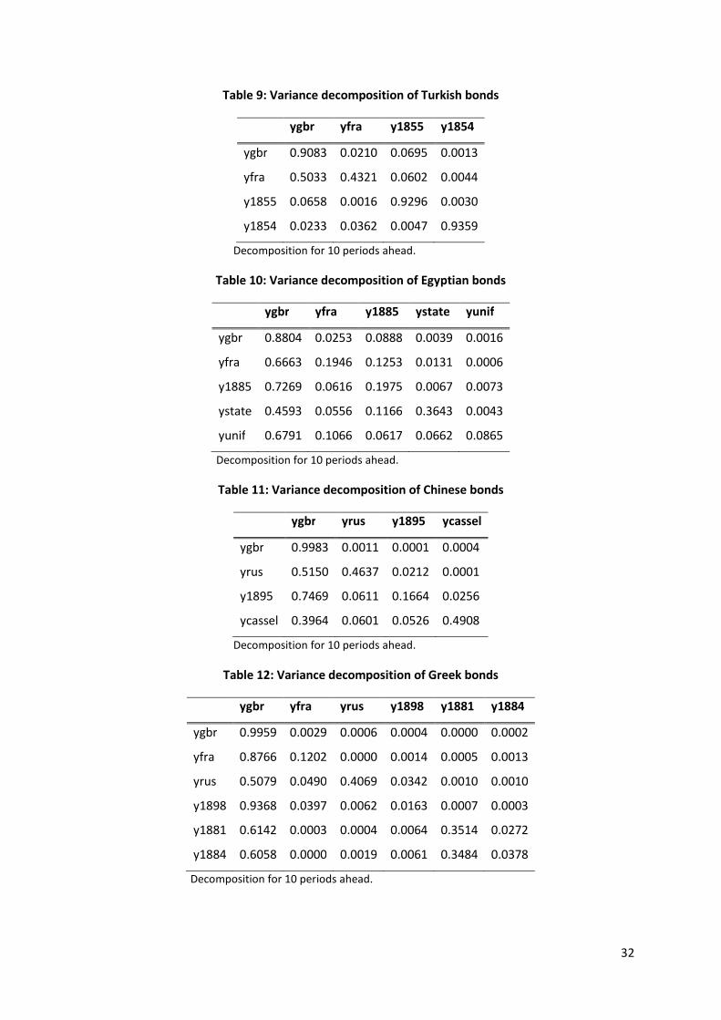
32

Table 9: Variance decomposition of Turkish bonds

Decomposition for 10 periods ahead.

Table 10: Variance decomposition of Egyptian bonds

ygbr yfra y1885 ystate yunif

ygbr 0.8804 0.0253 0.0888 0.0039 0.0016

yfra 0.6663 0.1946 0.1253 0.0131 0.0006

y1885 0.7269 0.0616 0.1975 0.0067 0.0073

ystate 0.4593 0.0556 0.1166 0.3643 0.0043

yunif 0.6791 0.1066 0.0617 0.0662 0.0865

Decomposition for 10 periods ahead.

Table 11: Variance decomposition of Chinese bonds

ygbr yrus y1895 ycassel

ygbr 0.9983 0.0011 0.0001 0.0004

yrus 0.5150 0.4637 0.0212 0.0001

y1895 0.7469 0.0611 0.1664 0.0256

ycassel 0.3964 0.0601 0.0526 0.4908

Decomposition for 10 periods ahead.

Table 12: Variance decomposition of Greek bonds

ygbr yfra yrus y1898 y1881 y1884

ygbr 0.9959 0.0029 0.0006 0.0004 0.0000 0.0002

yfra 0.8766 0.1202 0.0000 0.0014 0.0005 0.0013

yrus 0.5079 0.0490 0.4069 0.0342 0.0010 0.0010

y1898 0.9368 0.0397 0.0062 0.0163 0.0007 0.0003

y1881 0.6142 0.0003 0.0004 0.0064 0.3514 0.0272

y1884 0.6058 0.0000 0.0019 0.0061 0.3484 0.0378

Decomposition for 10 periods ahead.

ygbr yfra y1855 y1854

ygbr 0.9083 0.0210 0.0695 0.0013

yfra 0.5033 0.4321 0.0602 0.0044

y1855 0.0658 0.0016 0.9296 0.0030

y1854 0.0233 0.0362 0.0047 0.9359

33

Figure 1: Greek bonds, 1832-34

Figure 2: Turkish bonds, 1854-56

4.2

4.4

4.6

4.8

55

.2

10

15

20

25

30

%

01/1

/183

2

01/4

/183

2

01/7

/183

2

01/1

0/18

32

01/1

/183

3

01/4

/183

3

01/7

/183

3

01/1

0/18

33

01/1

/183

4

01/4

/183

4

01/7

/183

4

01/1

0/18

34

Structural breaks 1825 independence loan (LHS)

1833 loan (UK) 1833 loan (Rus)

1833 loan (Fra)

Structural breaks at 5% significance with 95% confidence intervals from Bai and Perron (1998)

45

67

8%

01/7

/185

4

01/1

0/18

54

01/1

/185

5

01/4

/185

5

01/7

/185

5

01/1

0/18

55

01/1

/185

6

01/4

/185

6

01/7

/185

6

01/1

0/18

56

01/1

/185

7

Structural breaks 6% 1854 loan

4% Guaranteed loan 1855

Structural breaks at 5% significance with 95% confidence intervals from Bai and Perron (1998)

34

Figure 3: Egyptian bonds, 1884-85

Figure 4: Chinese bonds, 1895

34

56

7%

01/1

/188

4

01/4

/188

4

01/7

/188

4

01/1

0/18

84

01/1

/188

5

01/4

/188

5

01/7

/188

5

01/1

0/18

85

01/1

/188

6

Structural breaks 4% Unified 1880

5% State Domain 1878 3% Guaranteed 1885

Structural breaks at 5% significance with 95% confidence intervals from Bai and Perron (1998)

44

.55

5.5

6%

01/5

/189

5

01/6

/189

5

01/7

/189

5

01/8

/189

5

01/9

/189

5

01/1

0/18

95

01/1

1/18

95

01/1

2/18

95

01/1

/189

6

Structural breaks 6% Cassel 1895

4% Guaranteed 1895

Structural breaks at 5% significance with 95% confidence intervals from Bai and Perron (1998)

35

Figure 5: Greek bonds, 1898-99

2.5

33

.54

4.5

5%

01/1

/189

8

01/3

/189

8

01/5

/189

8

01/7

/189

8

01/9

/189

8

01/1

1/18

98

01/1

/189

9

01/3

/189

9

01/5

/189

9

01/7

/189

9

01/9

/189

9

Structural breaks 5% loan 1881

5% loan 1884 2.5% Guaranteed 1898

Structural breaks at 5% significance with 95% confidence intervals from Bai and Perron (1998)

36

Figure 6: Long-term difference ro - rg

Figure 7: Factor loadings for Egypt and Greece

Default

10

02

00

30

04

00

50

0b

ps

1/1868

1/1870

1/1872

1/1874

1/1876

1/1878

1/1880

1/1882

1/1884

1/1886

1/1888

1/1890

1/1892

1/1894

Ottoman Empire

50

10

01

50

20

02

50

30

0b

ps

1/1886

1/1888

1/1890

1/1892

1/1894

1/1896

1/1898

1/1900

1/1902

1/1904

1/1906

1/1908

Egypt

50

10

01

50

20

02

50

bp

s

1/1895

1/1896

1/1897

1/1898

1/1899

1/1900

1/1901

1/1902

1/1903

1/1904

1/1905

1/1906

1/1907

China

15

02

00

25

03

00

35

0b

ps

1/1898

1/1899

1/1900

1/1901

1/1902

1/1903

1/1904

1/1905

1/1906

1/1907

Greece

ygbr

yfra

ytm85

ytmstateyunif

0.2

.4.6

.81

Fa

cto

r 2

0 .2 .4 .6 .8 1Factor 1

Rotation: orthogonal varimaxMethod: principal factors

Factor loadings

ygbr

yfra

yrus

ytm98

ytm81ytm84

.2.4

.6.8

1

Fa

cto

r 2

.2 .4 .6 .8 1Factor 1

Rotation: orthogonal varimaxMethod: principal factors

Factor loadings

Left: Egypt, 1886-1907. Right: Greece, 1898-1907

37

Figure 8: Impulse Response Functions for Turkey 1855

Figure 9: Impulse Response Functions for China 1895

Impulse-responses for 1 lag VAR of ygbr yfra ytm55 ytm54

Errors are 5% on each side generated by Monte-Carlo with 500 reps

response of ygbr to ygbr shocks

(p 5) ygbr ygbr (p 95) ygbr

0 6

0.0000

0.0730

response of ygbr to yfra shocks

(p 5) yfra yfra (p 95) yfra

0 6

0.0000

0.0375

response of ygbr to ytm55 shocks

(p 5) ytm55 ytm55 (p 95) ytm55

0 6

-0.0827

0.0032

response of ygbr to ytm54 shocks

(p 5) ytm54 ytm54 (p 95) ytm54

0 6

-0.0043

0.0227

response of yfra to ygbr shocks

(p 5) ygbr ygbr (p 95) ygbr

0 6

0.0000

0.0934

response of yfra to yfra shocks

(p 5) yfra yfra (p 95) yfra

0 6

0.0000

0.1180

response of yfra to ytm55 shocks

(p 5) ytm55 ytm55 (p 95) ytm55

0 6

-0.1677

0.0599

response of yfra to ytm54 shocks

(p 5) ytm54 ytm54 (p 95) ytm54

0 6

-0.0200

0.0626

response of ytm55 to ygbr shocks

(p 5) ygbr ygbr (p 95) ygbr

0 6

-0.1268

0.0615

response of ytm55 to yfra shocks

(p 5) yfra yfra (p 95) yfra

0 6

-0.2625

0.0415

response of ytm55 to ytm55 shocks

(p 5) ytm55 ytm55 (p 95) ytm55

0 6

0.0000

0.7503

response of ytm55 to ytm54 shocks

(p 5) ytm54 ytm54 (p 95) ytm54

0 6

-0.1860

0.0414

response of ytm54 to ygbr shocks

(p 5) ygbr ygbr (p 95) ygbr

0 6

-0.3058

0.8928

response of ytm54 to yfra shocks

(p 5) yfra yfra (p 95) yfra

0 6

-0.5055

1.4158

response of ytm54 to ytm55 shocks

(p 5) ytm55 ytm55 (p 95) ytm55

0 6

-3.1516

1.4944

response of ytm54 to ytm54 shocks

(p 5) ytm54 ytm54 (p 95) ytm54

0 6

0.0000

1.5056

Impulse-responses for 1 lag VAR of ygbr yrus ytm95 ytmcs

Errors are 5% on each side generated by Monte-Carlo with 500 reps

response of ygbr to ygbr shocks

(p 5) ygbr ygbr (p 95) ygbr

0 6

0.0000

0.0824

response of ygbr to yrus shocks

(p 5) yrus yrus (p 95) yrus

0 6

-0.0102

0.0176

response of ygbr to ytm95 shocks

(p 5) ytm95 ytm95 (p 95) ytm95

0 6

-0.0116

0.0112

response of ygbr to ytmcs shocks

(p 5) ytmcs ytmcs (p 95) ytmcs

0 6

-0.0284

0.0301

response of yrus to ygbr shocks

(p 5) ygbr ygbr (p 95) ygbr

0 6

0.0000

0.0719

response of yrus to yrus shocks

(p 5) yrus yrus (p 95) yrus

0 6

0.0000

0.0827

response of yrus to ytm95 shocks

(p 5) ytm95 ytm95 (p 95) ytm95

0 6

-0.0038

0.0322

response of yrus to ytmcs shocks

(p 5) ytmcs ytmcs (p 95) ytmcs

0 6

-0.0294

0.0377

response of ytm95 to ygbr shocks

(p 5) ygbr ygbr (p 95) ygbr

0 6

0.0000

0.0774

response of ytm95 to yrus shocks

(p 5) yrus yrus (p 95) yrus

0 6

0.0000

0.0342

response of ytm95 to ytm95 shocks

(p 5) ytm95 ytm95 (p 95) ytm95

0 6

0.0000

0.0518

response of ytm95 to ytmcs shocks

(p 5) ytmcs ytmcs (p 95) ytmcs

0 6

-0.0131

0.0453

response of ytmcs to ygbr shocks

(p 5) ygbr ygbr (p 95) ygbr

0 6

0.0000

0.0764

response of ytmcs to yrus shocks

(p 5) yrus yrus (p 95) yrus

0 6

-0.0062

0.0698

response of ytmcs to ytm95 shocks

(p 5) ytm95 ytm95 (p 95) ytm95

0 6

-0.0064

0.0532

response of ytmcs to ytmcs shocks

(p 5) ytmcs ytmcs (p 95) ytmcs

0 6

0.0000

0.1201

38

Figure 10: Impulse Response Functions for Egypt 1885

Impulse-responses for 1 lag VAR of ygbr yfra ytm85 ytmstate yunif

Errors are 5% on each side generated by Monte-Carlo with 500 reps

response of ygbr to ygbr shocks

(p 5) ygbr ygbr (p 95) ygbr

0 6

0.0000

0.2154

response of ygbr to yfra shocks

(p 5) yfra yfra (p 95) yfra

0 6

-0.0083

0.0646

response of ygbr to ytm85 shocks

(p 5) ytm85 ytm85 (p 95) ytm85

0 6

-0.0198

0.1494

response of ygbr to ytmstate shocks

(p 5) ytmstate ytmstate (p 95) ytmstate

0 6

-0.0132

0.0542

response of ygbr to yunif shocks

(p 5) yunif yunif (p 95) yunif

0 6

-0.0196

0.0042

response of yfra to ygbr shocks

(p 5) ygbr ygbr (p 95) ygbr

0 6

0.0000

0.2191

response of yfra to yfra shocks

(p 5) yfra yfra (p 95) yfra

0 6

0.0000

0.0955

response of yfra to ytm85 shocks

(p 5) ytm85 ytm85 (p 95) ytm85

0 6

-0.0135

0.1696

response of yfra to ytmstate shocks

(p 5) ytmstate ytmstate (p 95) ytmstate

0 6

-0.0098

0.0623

response of yfra to yunif shocks

(p 5) yunif yunif (p 95) yunif

0 6

-0.0172

0.0112

response of ytm85 to ygbr shocks

(p 5) ygbr ygbr (p 95) ygbr

0 6

0.0000

0.2189

response of ytm85 to yfra shocks

(p 5) yfra yfra (p 95) yfra

0 6

0.0000

0.0775

response of ytm85 to ytm85 shocks

(p 5) ytm85 ytm85 (p 95) ytm85

0 6

-0.0071

0.1680

response of ytm85 to ytmstate shocks

(p 5) ytmstate ytmstate (p 95) ytmstate

0 6

-0.0111

0.0570

response of ytm85 to yunif shocks

(p 5) yunif yunif (p 95) yunif

0 6

-0.0261

0.0000

response of ytmstate to ygbr shocks

(p 5) ygbr ygbr (p 95) ygbr

0 6

0.0000

0.1659

response of ytmstate to yfra shocks

(p 5) yfra yfra (p 95) yfra

0 6

-0.0027

0.0655

response of ytmstate to ytm85 shocks

(p 5) ytm85 ytm85 (p 95) ytm85

0 6

-0.0087

0.1348

response of ytmstate to ytmstate shocks

(p 5) ytmstate ytmstate (p 95) ytmstate

0 6

0.0000

0.0850

response of ytmstate to yunif shocks

(p 5) yunif yunif (p 95) yunif

0 6

-0.0112

0.0157

response of yunif to ygbr shocks

(p 5) ygbr ygbr (p 95) ygbr

0 6

0.0000

0.2077

response of yunif to yfra shocks

(p 5) yfra yfra (p 95) yfra

0 6

0.0000

0.0809

response of yunif to ytm85 shocks

(p 5) ytm85 ytm85 (p 95) ytm85

0 6

-0.0217

0.1473

response of yunif to ytmstate shocks

(p 5) ytmstate ytmstate (p 95) ytmstate

0 6

0.0000

0.0726

response of yunif to yunif shocks

(p 5) yunif yunif (p 95) yunif

0 6

0.0000

0.0385

39

Figure 11: Impulse Response Functions for Greece 1898

Impulse-responses for 1 lag VAR of ygbr yfra yrus ytm98 ytm81 ytm84

Errors are 5% on each side generated by Monte-Carlo with 500 reps

response of ygbr to ygbr shocks

(p 5) ygbr ygbr (p 95) ygbr

0 6

0.0000

0.0781

response of ygbr to yfra shocks

(p 5) yfra yfra (p 95) yfra

0 6

-0.0055

0.0122

response of ygbr to yrus shocks

(p 5) yrus yrus (p 95) yrus

0 6

-0.0047

0.0095

response of ygbr to ytm98 shocks

(p 5) ytm98 ytm98 (p 95) ytm98

0 6

-0.0080

0.0069

response of ygbr to ytm81 shocks

(p 5) ytm81 ytm81 (p 95) ytm81

0 6

-0.0068

0.0099

response of ygbr to ytm84 shocks

(p 5) ytm84 ytm84 (p 95) ytm84

0 6

-0.0044

0.0034

response of yfra to ygbr shocks

(p 5) ygbr ygbr (p 95) ygbr

0 6

0.0000

0.0741

response of yfra to yfra shocks

(p 5) yfra yfra (p 95) yfra

0 6

0.0000

0.0275

response of yfra to yrus shocks

(p 5) yrus yrus (p 95) yrus

0 6

-0.0076

0.0076

response of yfra to ytm98 shocks

(p 5) ytm98 ytm98 (p 95) ytm98

0 6

-0.0080

0.0013

response of yfra to ytm81 shocks

(p 5) ytm81 ytm81 (p 95) ytm81

0 6

-0.0076

0.0060

response of yfra to ytm84 shocks

(p 5) ytm84 ytm84 (p 95) ytm84

0 6

-0.0013

0.0064

response of yrus to ygbr shocks

(p 5) ygbr ygbr (p 95) ygbr

0 6

0.0000

0.0709

response of yrus to yfra shocks

(p 5) yfra yfra (p 95) yfra

0 6

0.0000

0.0285

response of yrus to yrus shocks

(p 5) yrus yrus (p 95) yrus

0 6

0.0000

0.0840

response of yrus to ytm98 shocks

(p 5) ytm98 ytm98 (p 95) ytm98

0 6

-0.0016

0.0398

response of yrus to ytm81 shocks

(p 5) ytm81 ytm81 (p 95) ytm81

0 6

-0.0127

0.0262

response of yrus to ytm84 shocks

(p 5) ytm84 ytm84 (p 95) ytm84

0 6

-0.0112

0.0129

response of ytm98 to ygbr shocks

(p 5) ygbr ygbr (p 95) ygbr

0 6

0.0000

0.0760

response of ytm98 to yfra shocks

(p 5) yfra yfra (p 95) yfra

0 6

0.0000

0.0188

response of ytm98 to yrus shocks

(p 5) yrus yrus (p 95) yrus

0 6

-0.0006

0.0125

response of ytm98 to ytm98 shocks

(p 5) ytm98 ytm98 (p 95) ytm98

0 6

-0.0039

0.0204

response of ytm98 to ytm81 shocks

(p 5) ytm81 ytm81 (p 95) ytm81

0 6

-0.0039

0.0089

response of ytm98 to ytm84 shocks

(p 5) ytm84 ytm84 (p 95) ytm84

0 6

-0.0028

0.0049

response of ytm81 to ygbr shocks

(p 5) ygbr ygbr (p 95) ygbr

0 6

0.0000

0.0811

response of ytm81 to yfra shocks

(p 5) yfra yfra (p 95) yfra

0 6

-0.0189

0.0129

response of ytm81 to yrus shocks

(p 5) yrus yrus (p 95) yrus

0 6

-0.0187

0.0274

response of ytm81 to ytm98 shocks

(p 5) ytm98 ytm98 (p 95) ytm98

0 6

-0.0313

0.0100

response of ytm81 to ytm81 shocks

(p 5) ytm81 ytm81 (p 95) ytm81

0 6

0.0000

0.0716

response of ytm81 to ytm84 shocks

(p 5) ytm84 ytm84 (p 95) ytm84

0 6

-0.0010

0.0340

response of ytm84 to ygbr shocks

(p 5) ygbr ygbr (p 95) ygbr

0 6

0.0000

0.0806

response of ytm84 to yfra shocks

(p 5) yfra yfra (p 95) yfra

0 6

-0.0182

0.0142

response of ytm84 to yrus shocks

(p 5) yrus yrus (p 95) yrus

0 6

-0.0160

0.0307

response of ytm84 to ytm98 shocks

(p 5) ytm98 ytm98 (p 95) ytm98

0 6

-0.0304

0.0102

response of ytm84 to ytm81 shocks

(p 5) ytm81 ytm81 (p 95) ytm81

0 6

0.0000

0.0730

response of ytm84 to ytm84 shocks

(p 5) ytm84 ytm84 (p 95) ytm84

0 6

-0.0007

0.0357

40

Figure A.1: Alternative yields of Egyptian 3% guaranteed bond of 1885

6. References

6.1 Primary Sources

Bulletin de la Cote, Compagnie des agents de chance, accessed at http://www.gallica.fr

CFB, Council of the Corporation of Foreign Bondholders, Annual Reports, 1874-1914

FO, Foreign Office Papers, National Archives, London

HCH, House of Commons Hansard, 1803-1914

HCPP, House of Commons Parliamentary Papers, 1800-1914

HMT, HM Treasury Reports, National Archives, London

IMM, Investor’s Monthly Manual, accessed at http://som.yale.edu/faculty-research/our-centers-

initiatives/international-center-finance/data/historical-london

RA, The Rothschild Archive, London.

Tableau des titres cotés à la Bourse de Paris, Direction générale de l’enregistrement, des domaines

et du timbre.

22.5

33.5

%

1/18

86

1/18

88

1/18

90

1/18

92

1/18

94

1/18

96

1/18

98

1/19

00

1/19

02

1/19

04

1/19

06

1/19

08

Simple yield YTM YTC

Monthly data. Source: IMM.

41

Times Digital Archive 1785-2006, Farmington Hills, Mich.: Thomson-Gale.

The Economist Historical Archive, 1843-2007, Gale Group.

The Course of the Exchange, 1832-1899, London, Guildhall Library.

6.2 Secondary Sources

Accominotti, O. et al. (2010) “Black Man's Burden, White Man's Welfare: Control, Devolution and

Development in the British Empire, 1880-1914,” European Review of Economic History 14(1): 47-

70.

Akar, S. K. and H. Al, H. (2003) Osmanlı Dış Borçları ve Gözetim Komisyonları, 1854-1856, Istanbul.

Al, H. (2007) Uluslararası Sermaye ve Osmanlı Maliyesi : 1820-1875, Istanbul.

Anderson, O. (1964) “Great Britain and the Beginnings of the Ottoman Public Debt, 1854-55”, The

Historical Journal, VII(I): 47-63

Andreades, A. (1925) Les contrôles financiers internationaux, Paris: Librairie Hachette.

Angeloni, C., and G. Wolff,(2012) “Are Banks Affected by Their Holdings of Government Debt?”

Bruegel Working Paper 2012/07.

Arellano, M. and S. Bond. (1991) “Some tests of specification for panel data: Monte Carlo evidence

and an application to employment equations,” Review of Economic Studies, 58(2): 277-297.

Arellano, M. and O. Bover (1995) “Another look at the instrumental variable estimation error

component models,” Journal of Econometrics, 68(10): 29-51.

Asquith, P. and D. Mullins (1986) “Equity Issues and Offering Dilution,” Journal of Financial

Economics, 15: 61-89.

Bai, J. and P. Perron (1998) “Estimating and testing linear models with multiple structural changes,”

Econometrica 66: 47-78.

Bai, J. and P. Perron (2003) “Computation and analysis of multiple structural change models,”

Journal of Applied Econometrics 18: 1-22.

Barclays Capital Economic Research (2011) “Euro Themes, A proposal to restore euro area stability,”

18 August 2011.

Bofinger, P. et al. (2011) “A European Redemption Pact,” VoxEU, 11November.

Bolton, P. and O. Jeanne (2009) “Structuring and Restructuring Sovereign Debt: The Role of

Seniority,” Review of Economic Studies 76: 879–902.

Boonstra, W.W. (2010) “The Creation of a Common European Bond Market,” Cahier Comte Boël, No.

14, ELEC.

Borchard, E. (1951) State Insolvency and Foreign Bondholders: General Principles, Yale: Yale

University Press.

Brunnermeier, M., L. Garicano, P. Lane, M. Pagano, R. Reis, T. Santos, S. van Nieuwerburgh, and D.

Vayanos (2011) “ESBies: A realistic reform of Europe's financial architecture,” VoxEU, 25 October.

Cannon, B. D. (1972) “A reassessment of judicial reform in Egypt, 1876-1891”, International Journal

of African Historical Studies, 5(1): 51-74.

Choi, I. (2001) “Unit root tests for panel data,” Journal of International Money and Finance, 20: 249-

272.

Claessens, S., A. Mody and S. Vallée (2012) “Paths to Eurobonds,” IMF Working Paper 12/172.

Collet, S. (2012) Sovereign Bonds: Odious Debts and State Succession, PhD Dissertation, Université

42

Libre de Bruxelles.

Cottarelli, C. and C. Giannini (2002) “Bedfellows, Hostages, or Perfect Strangers?: Global Capital

Markets and the Catalytic Effect of IMF Crisis Lending”, IMF Working Paper 02/193.

Crouchley, A. E. (1938) The economic development of modern Egypt, London: Longmans.

Delpla, J. and J. von Weizsäcker (2010) “The Blue Bond Proposal,” Breugel Policy Briefs 420, Bruegel,

Brussels.

De Grauwe, P. and W. Moesen (2009) “Gains for all: a proposal for a common euro bond,”

Intereconomics, May/June: 132 – 135.

Delors, J. (1989) “Report on Economic and Monetary Union in the European Community,” presented

April 17, 1989 by Committee for the Study of Economic and Monetary Union.

Denby, C. (1916) “The National Debt of China–Its Origin and Its Security,” Annals of the American

Academy of Political and Social Science, 68: 55-70.

Detragiache, E. (1994) “Sensible Buybacks of Sovereign Debt”, Journal of Development Economics 43,

317-333.

Deville, F. (1912), Les contrôles financiers internationaux et la souveraineté de l'état, Paris: Limoges.

Dübel, H.-J. (2011) “Partial sovereign bond insurance by the eurozone: A more efficient alternative

to blue (Euro-)bonds,” CEPS Policy Brief No. 252.

Eichengreen, B. and A. Mody (2000) “Lending Booms, Reserves, and the Sustainability of Short-Term

Debt: Inferences from the Pricing of Syndicated Bank Loans,” Journal of Development Economics,

63(1): 5-44.

EPDA/SIFMA (2009) “Towards a Common European T-bill,” Briefing Note March 2009.

Esteves, R. (2013) “The Bondholder, the Sovereign, and the Banker. Sovereign Debt and

Bondholders' Protection Before 1914,” European Review of Economic History, 17 (4): 389-407.

European Commission (2011) “Green Paper on the Feasibility of Introducing Stability Bonds,”

November 23.

Fama, E. and M. Miller (1972) The Theory of Finance, New York: Holt, Rinehart and Winston.

Favero, C. and A. Missale (2011) “Sovereign Spreads in the Euro Area. Which Prospects for a

Eurobond?” CEPR Discussion Paper #8637.

Feng-Hua H. (1919) Public Debts in China, New York: AMS Press.

Fenn, C. (1883) Fenn's Compendium of the English and Foreign Funds, Debts and Revenues of All

Nations, London.

Flandreau, M. (2013) “Collective Action Clauses before they had Airplanes: Bondholder Committees

and the London Stock Exchange in the 19th Century (1827-1868)” Graduate Institute of

International and Development Studies Working Paper No: 01/2013.

Flandreau, M. and J. Flores (2009) “Bonds and Brands: Foundations of Sovereign Debt Markets,

1820–1830” The Journal of Economic History 69(3): 648-84.

Flandreau, M., J. Le Cacheux and F. Zumer (1998) “Stability without a pact? Lessons from the

European gold standard, 1880–1914,” Economic Policy 13(26): 115-62.

Flandreau, M. And F. Zumer (2004) Making of Global Finance, 1880-1913, Paris: OECD.

Gros, D. (2010) “The Seniority Conundrum. Bail out countries but bail in private, short-term

creditors?” CEPS Commentary, 6 December 2010, Brussels: Centre for European Policy Studies.

Gros, D. (2011) “Eurobonds: Wrong Solution for Legal, Political, and Economic Reasons,” VoxEU, 24

August.

Hatchondo, J., L. Martinez and C. Padilla (2012) “Debt dilution and sovereign default risk” FRB

Richmond Working Paper 10-08R.

43

Holtz-Eaking, D., W. Newey and H. Rosen (1988) “Estimating vector autoregressions with panel

data,” Econometrica, 56(6): 1371-1395.

Hoyle, M. S. W. (1986) “The mixed courts of Egypt 1875-1885”, Arab Law Quarterly, 1(4): 436-451.

Hyde, C. C. (1922) “The Negotiation of External Loans with Foreign Governments”, American Journal

of International Law, 16(4): 523-41.

Issing, O. (2009) “Why a Common Eurozone Bond Isn't Such a Good Idea,” White Paper No. 3, Centre

for Financial Studies, Frankfurt.

Jeze, G. (1924) La garantie des rmprunts publics d’Etat, Paris.

Kimber, A. (1920) Kimber's Record of Government Debts, New York.

Kiray, E. Z. (1988) Foreign Debt and Structural Change in the" Sick Man of Europe" –the Ottoman

Empire, 1850-1875, PhD Thesis, MIT.

Kofas, J. V. (1981) Financial Relations of Greece and the Great powers, 1832-1862, New York:

Columbia University Press.

Kopf, Christian (2011) “Restoring Financial Stability in the Euro Area,” CEPS Policy Brief No. 237, 15

March 2011.

Levandis, J. A. (1944) The Greek Foreign Debt and the Great powers, 1821-1898, New York: Columbia

University Press.

MacMurray, J. V. A. (1921) Treaties and Agreements with and concerning China, 1894-1914, Oxford:

Oxford University Press.

Masulis (1980) “The Effects of Capital Structure Change on Security Prices,” Journal of Financial

Economics, 8: 139-78.

Mauro, P., N. Sussman and Y. Yafeh (2006) Emerging Markets and Financial Globalization. Sovereign

Spreads in 1870-1913 and Today, Oxford: Oxford University Press.

Mitchener, K. and M. Weidenmier (2010) “Supersanctions and Sovereign Debt Repayment,” Journal

of International Money and Finance 29: 19-36.

Mody, A. and D. Saravia, (2003) “Catalyzing Capital Flows: Do IMF-Supported Programs Work as

Commitment Devices?” IMF working paper WP/100/03.

Muellbauer, J. (2011) “Time for Eurobonds – but with conditions,” VoxEU, 12 October.

Muellbauer, J. (2013) “Conditional Eurobonds and the Eurozone Sovereign Debt Crisis,” Oxford

Review of Economic Policy 29(4).

NATIXIS (2011) “What bonus/penalty system for the Stability Bond?” Flash Economics No 613, 22

August 2011.

Neal, L. (1998) “The financial crisis of 1825 and the restructuring of the British financial system”

Federal Reserve Bank of St Louis Review, 80(3): 53-76.

Neal, L. and L. Davis (2006) “The Evolution of the Structure and Performance of the London Stock

Exchange in the First Global Financial Market, 1812-1914”, European Review of Economic History,

Vol 10, no. 3.

Roubini, N. and B. Setser (2004) Bailouts or Bail-ins? Responding to Financial Crises in Emerging

Economies, Washington, DC: Peterson Institute.

Saravia, D. (2010) "On the role and effects of IMF seniority," Journal of International Money and

Finance 29(6): 1024-1044.

Schwartz, A. (1997) “Priority Contracts and Priority in Bankruptcy”, Cornell Law Review 82: 1396-

1435.

Suter, C. (1992) Debt Cycles in the World-Economy: Foreign Loans, Financial Crises, and Debt

Settlements, 1820-1990, Boulder: Westview Press.

44

Tirole, J. (2002) Financial Crises, Liquidity Provision and the International Monetary System,

Princeton: Princeton University Press.

Tuncer, A. C. (2011) Fiscal autonomy, monetary regime and sovereign risk, PhD Thesis, University of

London.

Uribe, M. and V. Yue (2006) “Country Spreads and Emerging Countries: Who Drives Whom?” Journal

of International Economics 69(1): 6-36.

White, M. (1980) “Public Policy towards Bankruptcy: Me-first and other Priority Rules”, Bell Journal

of Economics 11: 550-564.

Viner, J. (1928) “Political Aspects of International Finance” The Journal of Business of the University

of Chicago, 1(3): 324-363.

Wynne, W. (1951) State Insolvency and Foreign Bondholders. Vol. II Selected Case Histories of

Governmental Foreign Bond Defaults and Debt Readjustments, Yale: Yale University Press.