Fermions And Topological Phases, II

Edward Witten

PSCCMP/PiTP Lectures

Last time we talked about Weyl fermions in condensed matter andthe boundary-localized modes that they produce. It is also possibleto get boundary-localized modes from Dirac fermions, and sincethis is important in understanding topological insulators, I will saya little about it.

In the absence of discrete symmetries, and without tuning anyparameters, it is not natural in condensed matter physics to get amassless Dirac (as opposed to Weyl) fermion. That is simplybecause for a four-component fermion field ψ with both chiralities,mass terms are possible, in fact there are two such terms:(

i∑µ

γµ∂µ −m −m′γ5

)ψ = 0.

To get a massless Dirac fermion, we need a reason form = m′ = 0. It turns out that it is actually possible to achieve thisin the context of a crystal with suitable discrete symmetries, butunfortunately there will not be time to explain this.

The only symmetry that we will assume is time-reversal symmetry,and this is enough to set one of the two parameters to 0 but notboth. The Dirac equation becomes(

i∑µ

γµ∂µ −m

)ψ = 0.

Generically m is not 0 but of course if we adjust one parameter (forexample the chemical composition of an alloy) we can hope to passthrough a point with m = 0. It turns out that this is the phasetransition between an ordinary insulator and a topological one. Fornow, we consider a sample with boundary and look for a modelocalized near the boundary.

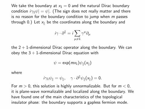
We take the boundary at x1 = 0 and the natural Dirac boundarycondition iγ1ψ| = ψ|. (The sign does not really matter and thereis no reason for the boundary condition to jump when m passesthrough 0.) Let x‖ be the coordinates along the boundary and

iγ · ∂‖ = i∑µ6=1

γµ∂µ

the 2 + 1-dimensional Dirac operator along the boundary. We canobey the 3 + 1-dimensional Dirac equation with

ψ = exp(mx1)ψ‖(x‖)

whereiγ1ψ‖ = ψ‖, γ · ∂‖ψ‖(x‖) = 0.

For m > 0, this solution is highly unnormalizable. But for m < 0,it is plane-wave normalizable and localized along the boundary. Wehave found one of the main characteristics of the topologicalinsulator phase: the boundary supports a gapless fermion mode.

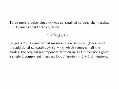
To be more precise, since ψ‖ was constrained to obey the massless2 + 1 dimensional Dirac equation

γ · ∂‖ψ‖(x‖) = 0,

we get a 2 + 1 dimensional massless Dirac fermion. (Because ofthe additional constraint iγ1ψ‖ = ψ‖ which removes half themodes, the original 4-component fermion in 3+1 dimensions givesa single 2-component massless Dirac fermion in 2 + 1 dimensions.)

Generically in the context of condensed matter physics the fermienergy εF does not pass through the Dirac point in the boundarytheory

so the boundary of a topological insulator is more like an ordinarymetal than some of the Weyl semimetals that we talked aboutyesterday.

To summarize the last point, we have learned that in a generic1-parameter family of T -conserving band theories, there can be aphase transition between a phase with no localized boundarymodes and a phase with a massless 2d fermion on the boundary.At the phase transition point, there is a massless 3d Dirac fermion.

As I have already remarked, the other way to get massless 3d Diracfermions in condensed matter is to take advantage of certaindiscrete crystal symmetries. This has actually been part of thebackground for some of the experimental talks that we have heard.

However, I want to go in a different direction involving anintroduction to some aspects of the integer quantum Hall effect.First I just want to explain from the point of view of effective fieldtheory why there is an integer quantum Hall effect in the firstplace. We consider a material that not only is an insulator, butmore than that has no relevant degrees of freedom – not eventopological ones – in the sense that its interaction with anelectromagnetic field can be described by an effective action forthe U(1) gauge field A only, without any additional degrees offreedom. (This would certainly not be true in a conductor, whoseinteraction with an electromagnetic field cannot be describedwithout including the charge carriers in the description, along withA. But more subtly, as we will discuss, it is not true in a fractionalquantum Hall system, whose effective field theory requirestopological degrees of freedom coupled to A.)

In a 3 + 1-dimensional material with no relevant degrees offreedom, the effective action for the electromagnetic field can haveall sorts of terms associated to various familiar effects. Forexample, ferromagnetism and ferroelectricity correspond to termsin the effective action that are linear in ~E or ~B

I ′ =

∫W3×R

(~a · ~E + ~b · ~B

).

(Here W3 is the spatial volume of the material and R parametrizesthe time, so the “world-volume” of the material is M4 = W3 × R.)Similarly, electric and magnetic susceptibilities correspond to termsbilinear in ~E or ~B:

I ′′ =

∫W3×R

(αijEiEj + βijBiBj) .

And so on.

All these terms are manifestly gauge-invariant in the sense thatthey are integrals of gauge-invariant functions – the integrands areconstructed only from ~E and ~B (and possibly their derivatives). In2 + 1 dimensions, there is a unique term that is gauge-invariantbut does not have this property. This is the Chern-Simons coupling

ICS =1

4π

∫M2×R

d3xεijkAi∂jAk .

The density εijkAi∂jAk that is being integrated is definitely notgauge-invariant, but the integral is gauge-invariant up to a totalderivative. In fact, under

Ai → Ai + ∂iφ,

we have

εijkAi∂jAk → εijkAi∂jAk + ∂i

(εijkφ∂jAk

).

Roughly speaking, this shows that ICS is gauge-invariant, but wehave to be more careful because electric charge quantization, witha field of charge 1 transforming as

ψ → e iφψ

means that we should consider φ to be defined only modulo 2π:

φ ∼= φ+ 2π.

Given this fact, the previous proof of gauge-invariance of ICS is notquite correct and we will be more careful in a moment.

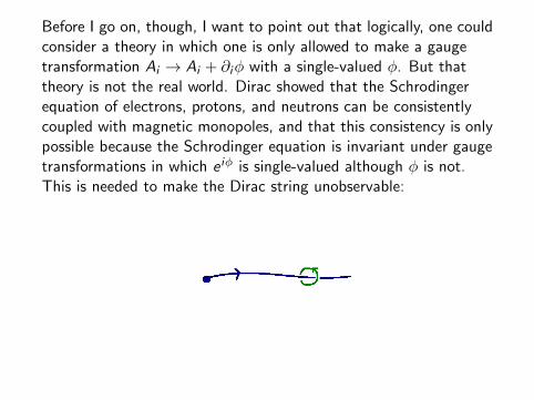
Before I go on, though, I want to point out that logically, one couldconsider a theory in which one is only allowed to make a gaugetransformation Ai → Ai + ∂iφ with a single-valued φ. But thattheory is not the real world. Dirac showed that the Schrodingerequation of electrons, protons, and neutrons can be consistentlycoupled with magnetic monopoles, and that this consistency is onlypossible because the Schrodinger equation is invariant under gaugetransformations in which e iφ is single-valued although φ is not.This is needed to make the Dirac string unobservable:

Anyway our microscopic knowledge that the Schrodinger equationis invariant under any gauge transformation such that e iφ issingle-valued (even if φ is not single-valued) implies constraints onthe effective action that we would not have without thatknowledge. We want to understand those constraints.

To do this, we will consider the following situation: we take ourtwo-dimensional material to be a closed two-manifold, for instanceS2, and we will take “time” to be a circle S1 of circumference β.(For example, we might be computing Tr e−βH .) Thus we considera material whose “worldvolume” is M3 = S2 × S1:

One might not be able to engineer this situation in the real worldbut it is clear that the Schdrodinger equation makes sense in thissituation. So we can consider it in deducing constraints on theeffective action that can arise from the Schrodinger equation.

The gauge field that we want to consider on M3 = S2 × S1 ischaracterized by the following: We place a unit of Dirac magneticflux on S2 ∫

S2

dx1dx2F

2π= 1.

(This is the right quantum of flux if the covariant derivative of theelectron is Diψ = (∂i − iAi )ψ, meaning that I am writing A forwhat is often called eA. This lets us avoid factors of e in manyformulas.) And we take a constant gauge field in the timedirection:

A0 =s

β

with constant s. (Remember the time direction is a circle ofcircumference β.) For this gauge field, one can calculate

ICS =1

4π

∫M3=S2×S1

d3xεijkAi∂jAk = s.

(This is actually a slightly tricky calculation.)

Note that the holonomy of A around the “time” circle is

exp

(i

∫ β

0A0dt

)= exp

(i

∫ β

0(s/β)dt

)= exp(is).

The gauge transformation

φ =2πt

β,

which was chosen to make e iφ periodic, acts by

s → s + 2π

and so leaves the holonomy invariant. (This must be true, becausewith my normalization of A, this holonomy is the phase factorwhen an electron is parallel-transported around the circle and so isphysically meaningful.)

So we have in this example ICS = s, and a gauge transformationcan act by s → s + 2π. So ICS is not quite gauge-invariant. Herewe must remember what is essentially the same fact that wasexploited by Dirac in his theory of the magnetic monopole. Theclassical action I enters quantum mechanics only via a factorexp(iI ) in the Feynman path integral (or exp(iI/~) if one restores~), so it is enough if I is well-defined and gauge-invariant mod2πZ. Since ICS is actually gauge-invariant mod 2πZ (we showedthis in an example but it is actually true in general), it can appearin the effective action with an integer coefficient:

Ieff = kICS + . . . .

The point of this explanation has been to explain why k has to bean integer – sometimes called the “level.” The fact that k is aninteger gives a macroscopic explanation of the quantization of theHall current. Indeed for any material whose interaction with anelectromagnetic potential A is governed by an effective action Ieff ,the induced current in the material is

Ji = −δIeff

δAi.

We are interested in the case that

Ieff = kICS =k

4π

∫M3

d3xεijkAi∂jAk .

Let us consider a material sitting at rest at x3 = 0 and thusparametrized by x1, x2.

The current in the x2 direction is

J2 = −δIeff

δA1=

kF012π

=kE1

2π.

This is called a Hall current: an electric field in the x1 direction hasproduced a current in the x2 direction. The Hall current has aquantized coefficient k/2π (usually called ke2/2π, recall that my Ais usually called eA; also I set ~ = 1 so h = 2π), where thequantization follows from the fact that ICS is not quitegauge-invariant.

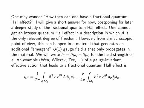
One may wonder “How then can one have a fractional quantumHall effect?” I will give a short answer for now, postponing for latera deeper study of the fractional quantum Hall effect. One cannotget an integer quantum Hall effect in a description in which A isthe only relevant degree of freedom. However, from a macroscopicpoint of view, this can happen in a material that generates anadditional “emergent” U(1) gauge field a that only propagates inthe material. We will write fij = ∂iaj − ∂jai for the field strength ofa. An example (Wen, Wilczek, Zee, ...) of a gauge-invarianteffective action that leads to a fractional quantum Hall effect is

Ieff =1

2π

∫M3

d3x εijkAi∂jak −r

4π

∫M3

d3x εijkai∂jak .

An oversimplified explanation of why this gives a fractionalquantum Hall effect is the following. One argues that as a appearsonly quadratically in the effective action, one can integrate it outusing its equation of motion. This equation is

f =1

rF ,

implying that up to a gauge transformation a = A/r . Substitutingthis in Ieff , we get an effective action for A only that describes afractional quantum Hall effect:

I ′eff =1

rICS(A) =

1

r

1

4π

∫M3

d3x εijkAi∂jAk .

Here 1/r appears where k usually does, and this suggests that theHall conductivity in this model is 1/r . That is correct. But thereclearly is something wrong with the derivation because the claimedanswer for the effective action I ′eff = (1/r)ICS(A) does not makesense as it violates gauge invariance. The mistake is that ingeneral, as F may have a flux quantum of 2π, and f has the sameallowed flux quantum (otherwise the action we assumed would notbe gauge-invariant), for a given A it is not possible to solve theequation

f =1

rF

for a. Thus, it is not possible to eliminate a from this system andgive a description in terms of A only. The reason that “integratingout a” gives the right answer for the Hall current is that thisprocedure is valid locally and this is enough to determine the Hallcurrent. The system has more subtle properties (fractionallycharged quasiparticles and topological degeneracies) that can onlybe properly understood in the description with a as well as A.

Going back to a theory that can be described in terms of A only,we have then an integer k in the macroscopic description. Butthere is also an integer in the microscopic description of a bandinsulator (Thouless-Kohmoto-Nightingale-den Nijs 1982). It arisesas follows. We consider a crystal with N bands, of which n arefilled. We assume the system is completely gapped.

say with n filled bands fand N − n empty bands. As we learnedyesterday, in a 2d system it is generic to have no band crossings.

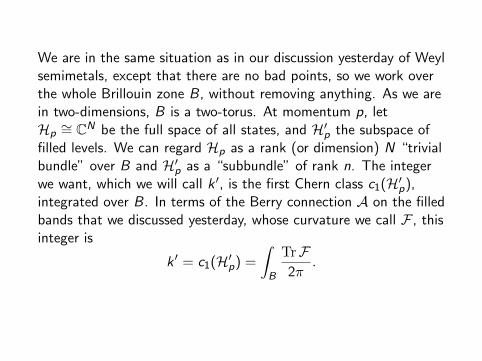
We are in the same situation as in our discussion yesterday of Weylsemimetals, except that there are no bad points, so we work overthe whole Brillouin zone B, without removing anything. As we arein two-dimensions, B is a two-torus. At momentum p, letHp∼= CN be the full space of all states, and H′p the subspace of

filled levels. We can regard Hp as a rank (or dimension) N “trivialbundle” over B and H′p as a “subbundle” of rank n. The integerwe want, which we will call k ′, is the first Chern class c1(H′p),integrated over B. In terms of the Berry connection A on the filledbands that we discussed yesterday, whose curvature we call F , thisinteger is

k ′ = c1(H′p) =

∫B

TrF2π

.

The basic claim of TKNN is that k ′, the flux of the Berryconnection, is the same as k , the coefficient of the quantum Hallcurrent. The original proof was based on literally just calculatingthe current from first principles in terms of a matrix element in thefermion ground state – which is written as an integral of singleparticle matrix elements over the Brillouin zone. I want to explaina different viewpoint that will emphasize that k ′ is not just a bandconcept but can be defined in the full many-body theory. (I hopeto describe tomorrow another approach essentially due to Haldaneto the relation k = k ′.)

We consider a finite sample, say on an L1 × L2 lattice

for very large L1, L2, where I will take lattice constants a1, a2 in thetwo directions. We assume periodic boundary conditions,maintaining the lattice translation symmetries. However, for thefinite system, the momenta take discrete values

p1 =2πs1a1L1

, 0 ≤ s1 ≤ L1 − 1

p2 =2πs2a2L2

, 0 ≤ s2 ≤ L2 − 1.

The ground state of the finite system is of course obtained byfilling all of the states in the first n bands with these values of themomenta.

Now, however, we turn on a background electromagnetic vectorpotential that is chosen such that the magnetic field vanishes, butan electron going all the way around the x1 direction or the x2direction picks up a phase:

A1 =α1

a1L1, A2 =

α2

a2L2.

The phase picked up by an electron going around the x1 (or x2)direction is exp(iα1) (or exp(iα2)) and up to a gaugetransformation the range of these parameters is

0 ≤ α1, α2 ≤ 2π.

From the point of view of band theory, the effect of turning on theparameters α1, α2 is just to shift the momenta of the electrons,which become

p1 =2πs1 + α1

a1L1, 0 ≤ s1 ≤ L1 − 1

p2 =2πs2 + α2

a2L2, 0 ≤ s2 ≤ L2 − 1.

This actually shows that the spectrum is invariant under a 2π shiftof α1 or of α2 (up to an integer shift of s1 or s2). For any α1, α2,from the point of view of band theory, the ground state is found byfilling all states in the first n bands with these shifted values of themomenta.

Now we think of the parameters α1, α2 as parameters that aregoing to vary adiabatically. Since they are each defined mod 2π,they parametrize a torus that I will call B. (B can be viewed as asort of rescaled version of the Brillouin zone B.) Since Berry’sconstruction is universal for adiabatic variation of parameters, wecan construct a Berry connection A over B, with curvature F . Ais a connection that can be used to transport the ground state asthe parameters α1, α2 are varied. All we need to know to define itis that the ground state is always nondegenerate as α1, α2 arevaried. We do not need to assume a single-particle picture (i.e.band theory). But I should say that for the conclusions we draw tobe useful, at least in the form I will state, we need the gap fromthe ground state to be independent of L1, L2 as they become large.(Otherwise in practice our measurements in the lab may not beadiabatic. The stated assumption is not true for a fractionalquantum Hall system, as I hope to explain tomorrow.)

Using the Berry connection over B, we can define an integer:

k ′ =

∫Bdα1 dα2

F2π.

But I claim that this is the same as the integer k ′ defined in bandtheory:

k ′ = k ′.

The reason that this is useful is that the definition of k ′ is moregeneral. To define k ′, we assume band theory – that is, asingle-particle description based on free electrons. The definition ofk ′ assumes much less.

To understand why k ′ = k ′, I have drawn

the discrete points in the Brillouin zone that obey the finite volumecondition

p1 =2πs1a1L1

, 0 ≤ s1 ≤ L1 − 1

p2 =2πs2a2L2

, 0 ≤ s2 ≤ L2 − 1.

at α1 = α2 = 0. The parameters α1, α2 parametrize one of thelittle rectangles in the picture, say the one at the lower left.

Turning on α1, α2 shifts the allowed momenta as shown.

To compute k ′, we integrate over B, the full Brillouin zone. Tocompute k ′, we integrate over the little rectangle, but for eachpoint in the little rectangle, we sum over the corresponding shiftedmomenta

These are two different ways to organize the same calculation, sok ′ = k ′.

So instead of proving the original TKNN formula k = k ′, we canprove k = k ′. This has the following advantage: k ′ is defined interms of the response of the system to a changing electromagneticvector potential A, so we can determine k ′ just from a knowledgeof the effective action for A.

As practice, before determining the Berry connection for A, I amgoing to determine the Berry connection for an arbitrary dynamicalsystem with dynamical variables x i (t). You can think of x i (t),i = 1, . . . , 3 as representing the position coordinates of a particle,but they really could be anything else (for example x i (t) couldhave 3N components representing the positions of N particles).Regardless, we assume an action

I =1

2

∫dt gij(x)

dx i

dt

dx j

dt+

∫dtAi (x)

dx i

dt−∫

dtV (x) + . . . .

(There might be higher order terms but it will be clear in amoment that they are not important.) We shall compute the Berryconnection in the space of semiclassical states of zero energy, acondition that we satisfy by imposing the condition V (x) = 0.(This semiclassical approximation is valid in our problem becausewe do not need to treat the electromagnetic vector potential Aquantum mechanically. We can view it as a given external field.)

Setting V = 0 means that we will evaluate the Berry phase not forall values of x but only for values of x that ensure V (x) = 0.

So we drop the V (x) term from the action, and only carry outtransport in the subspace of the configuration space with V = 0.In adiabatic transport, we can also ignore the term

Ikin =1

2

∫dt gij(x)

dx i

dt

dx j

dt

in the action, and any other term with two or more timederivatives. That is because if we transport from a starting point pto an ending point p′ in time T , the derivative dx i/dt is of order1/T , and Ikin ∼ 1/T .

So the only term in the action that we need to keep is the termwith precisely one time derivative:

I ′ =

∫dt Ai (x)

dx i

dt=

∫ p′

pAi (x)dx i .

As I have indicated, this term depends only on the path followedfrom p to p′, and not on how it is parametrized. Now rememberthat the phase that a quantum particle acquires in propagatingfrom p to p′ along a given trajectory is e iI/~, where I is the actionfor that trajectory.

For us this phase is just exp(i∫γ Aidx

i)

.

But the connection which on parallel transport along a path γ

gives a phase exp(i∫γ Aidx

i)

is just A. What we have learned, in

other words, is that for a system in which a quantum ground statecan be considered to be equivalent to a classical ground state, theBerry connection is just the classical connection A that can beread off from the classical action.

For the electromagnetic field in our problem, the action is

I =1

2e2

∫R3,1

d3xdt(~E 2 − ~B2

)+

k

4π

∫W3

d2xdt εijkAi∂jAk + . . .

We assume, for example, periodic boundary conditions with verylong periods L1, L2 in the two directions that are filled by ourquantum Hall sample. (It doesn’t matter if we assume periodicboundary conditions in the third direction.) A classical state ofzero energy is labeled by the two angles α1, α2 that wereintroduced before:

A1 =α1

a1L1, A2 =

α2

a2L2.

To compute the Berry phase, we are supposed to substitute thisformula in the action and keep only the part of the action that hasprecisely 1 time derivative. This comes only from theChern-Simons term.

After integration over x1 and x2, the relevant part of the action isjust

I ′ = − k

2π

∫dt α1

dα2

dt.

From this we read off the Berry connection

∇ ≡(

D

Dα1,

D

Dα2

)=

(∂

∂α1,∂

∂α2+ i

kα1

2π

)and hence the Berry curvature

Fα1α2 = −i[

D

Dα1,

D

Dα2

]=

k

2π.

(If we add to I ′ a total derivative term∫dt ∂t f (α1, α2), this will

change the formula for ∇ but it will not change F .)

We remember that the integer k ′ is supposed to be the integral ofF/2π over the Brillouin zone. We can now compute

k ′ =

∫ 2π

0dα1dα2

F2π

=

∫ 2π

0dα1dα2

k

(2π)2= k .

Thus we arrive at a version of the famous formula of TKNN: thecoefficient k of the quantum Hall current can be computed as aflux integral of the Berry connection. (A similar explanation can begiven for the result about the polarization of a 1-dimensionalsystem that Charlie Kane described in his first lecture. Also, let mesay again that the original proof that k = k ′ was based on a directevaluation of the Kubo formula for the conductivity in the contextof band theory.)

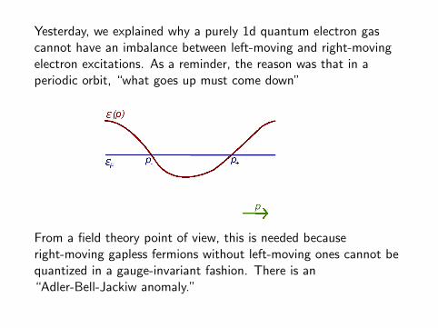
Yesterday, we explained why a purely 1d quantum electron gascannot have an imbalance between left-moving and right-movingelectron excitations. As a reminder, the reason was that in aperiodic orbit, “what goes up must come down”

From a field theory point of view, this is needed becauseright-moving gapless fermions without left-moving ones cannot bequantized in a gauge-invariant fashion. There is an“Adler-Bell-Jackiw anomaly.”

However, one of the hallmarks of a quantum Hall system is that onits boundary it has precisely such an imbalance. The reason thatthis must happen is that when we verified the invariance of theChern-Simons action

kICS =k

4π

∫M2×R

d3xεijkAi∂jAk

under a gauge transformation Ai → Ai + ∂iφ, we had to integrateby parts. This integration by parts produces a surface term on thesurface of our material – that is on ∂M2 ×R. There is not any wayto cancel this failure of gauge invariance by adding to the action asurface term supported on ∂M2 ×R. You can try to replace ICS by

ICS +

∫∂M2×R

dtdx (?????)

where ????? is some polynomial in A and its derivatives, butwhatever you try will not work. (I recommend this exercise.).

To cancel the “anomaly,” that is the failure of gauge invariance ofICS along the boundary, requires the existence on the boundary ofmodes that are (1) gapless, so they cannot be integrated out toproduce a local effective action for A only, and (2) “anomalous,”that is they are not possible in a purely 1-dimensional system.What fills the bill is precisely what we found does not exist in apurely 1-dimensional system: “chiral fermions,” that isright-moving gapless modes not accompanied by left-moving ones.

Since the failure of kICS is proportional to k , the “chiralasymmetry” that is needed to cancel it is also proportional to k . Infact, the hallmark of an integer quantum Hall system with a Hallconductivity of k is precisely that

n+ − n− = k

where n+ and n− are the numbers of “right-moving” and“left-moving” gapless edge modes. Instead of giving a technicalanalysis of field theory “anomalies” to explain how this works, Iwill give a couple of possibly more physical explanations – onetoday and hopefully one tomorrow.

Let us think of a quantum Hall system in the form of a longcylinder:

In fact for starters, think of an infinite cylinder.

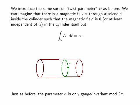
We introduce the same sort of “twist parameter” α as before. Wecan imagine that there is a magnetic flux α through a solenoidinside the cylinder such that the magnetic field is 0 (or at leastindependent of α) in the cylinder itself but∮

γA · d` = α.

Just as before, the parameter α is only gauge-invariant mod 2π.

We adiabatically increase α from 0 to 2π, with the scalar potentialassumed to be 0. Since the electric field is then

~E =∂ ~A

∂t,

increasing α turns on an electric field that goes “around” thecylinder. But in the case of a quantum Hall system, this drives acurrent that is perpendicular to ~E , in other words the current flows“along” the cylinder.

The electrons therefore are pushed to the left (or right, dependingon the sign of k).

An early explanation of the integer quantum Hall effect byLaughlin was the following. We assume that when α = 2π, thesystem returns to the same state that it was in at α = 0. (Thisassumption is not valid for fractional quantum Hall systems, asdiscussed later.) However, in the process, each electron may movek steps to the left, for some integer k . Notice that since thecylinder has a finite circumference S , the number of electrons perunit length is finite and thus it makes sense to say that each onemoves k steps to the left, for some k . This was interpreted as thebasic integrality of the integer quantum Hall effect. It does lead tothe value k/2π for the Hall conductivity.

Now let us consider a cylinder that is only semi-infinite, with aboundary at let us say the left end:

The same parameter α as before makes sense, and we can stilladiabatically increase it by 2π. Since a quantum Hall system isgapped, if we make a measurement far from the boundary, we willstill see the same flux of valence electrons to the left as before,assuming that only valence bands (states below the fermi energy)are filled.

But what happens to the electrons when they arrive at the leftboundary? A partial answer is that there are edge states, andelectrons go from the valence bands to the edge states. But this isnot enough: since the boundary has finite length, only finitelymany electrons can go into edge states (of reasonable energy).The only interpretation is that as electrons flow in to the left fromthe valence bands (the bands below the usual εF in the bulk) theymust eventually flow back out to the right in the conduction bands(the bands above the usual εF ). Moreover, all this is happeningcontinuously in energy so it must be possible for an electron toevolve continuously from the valence bands in the bulk, to theconduction bands in the bulk, somehow passing through edgestates.

The spectrum must therefore look something like this (drawn fork = 2):

Actually the edge states are a continuum, as drawn in the lastpicture, only in the limit that the circumference S of the cylindergoes to infinity. For a finite S , the spectrum of edge states isdiscrete, as shown here:

The little beads indicate “allowed states” of the edge modes, for agiven S and a given value of the angle α. As we adiabaticallyincrease α, each little bead moves up along the curve and underα→ α + 2π, each bead is shifted in position to the next one. Sounder α→ α+ 2π, there is a net charge flow of 1 from the valencebands to the conduction bands for each right-moving edge mode.

Recall that as we discussed yesterday, a 1d mode is rightmoving ifdε/dp > 0 at ε = εF . A left-moving mode has dε/dp < 0 atε = εF , and under α→ α + 2π produces a net charge flow of −1from the valence band to the conduction band. Thus with n+ andn− as the numbers of right- and left-moving modes, the net chargeflow under α→ α + 2π is

k = n+ − n−.

To tie up some loose ends: The 1d edge modes cannot be definedon the whole 1d Brillouin zone (which is a circle) because then wewould be stuck with the fact that in a periodic orbit “what goes upmust come down,” leading to n+ = n−. The asymmetry comesfrom branches of edge mode that exist in only a finite range ofmomenta p− ≤ p ≤ p+. What happens at the endpoints? Theanswer is the same as it was in a somewhat similar example thatwe looked at yesterday. The way that a family of edge-localizedstates can cease to exist at some momentum p− is by ceasing tobe normalizable. This happens when the edge state becomesindistinguishable from a bulk state.

That is part of what makes it possible to have adiabatic transportfrom the valence bands (the states normally filled) to theconduction bands (the states normally empty), through the edgestates. At the endpoint of the edge state spectrum, an edge stateis indistinguishable from a bulk state:

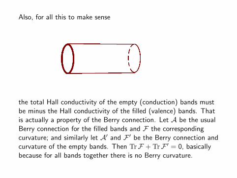
Also, for all this to make sense

the total Hall conductivity of the empty (conduction) bands mustbe minus the Hall conductivity of the filled (valence) bands. Thatis actually a property of the Berry connection. Let A be the usualBerry connection for the filled bands and F the correspondingcurvature; and similarly let A′ and F ′ be the Berry connection andcurvature of the empty bands. Then TrF + TrF ′ = 0, basicallybecause for all bands together there is no Berry curvature.

The Hall conductivities of filled and empty bands are respectively∫B

TrF2π

,

∫B

TrF ′

2π.

So the relation TrF + TrF ′ = 0 means that they have oppositeHall conductivities, and in our thought experiment, the flow of“filled” states (i.e. states that would be filled in the ground stateon an infinite cylinder) to the left equals the flow of “empty”states to the right.

I would like to explain the assertion that a fractional quantum Hallsystem does not return to its previous state under α→ α + 2π.We will use the same macroscopic model of a fractional quantumHall system that we used before in terms of the electromagneticvector potential A and an emergent U(1) gauge field a that onlyexists inside the material:

Ieff =1

2π

∫M3

d3x εijkAi∂jak −r

4π

∫M3

d3x εijkai∂jak .

First let us discuss how to characterize the state of the system fora given α

We recall that α was defined as∮γ A.

The parameter α =∮γ A can be controlled, in principle, by varying

the magnetic flux threaded by the cylinder. But there is ananalogous parameter

α =

∮γa

that cannot be controlled in that way. Just like α, α isgauge-invariant mod 2π.

What can we say about α? Recalling that F = dA, f = da are theordinary electromagnetic field strength and its analog for a, theclassical field equation for this system is

rf = F .

In the limit of an infinite cylinder, a can be treated classically. (Wepostpone the more interesting case of a finite cylinder untiltomorrow.) In the gauge A0 = a0 = 0, the equation rf0i = F0ibecomes

rdaidt

=dAi

dt,

and therefore

rdα

dt=

dα

dt.

Hence when we adiabatically increase α by 2π, α increasesadiabatically by 2π/r . Since α is gauge-invariant mod 2π, the shiftα→ α + 2π/r does not return the system to its original state. Weneed to take α→ α + 2πr , and therefore the Hall conductivity canbe smaller than its usual “quantum” by a factor of r .

The picture

still has some sort of analog, but the edge states cannot be freeelectron states: They have to be capable of transporting afractional current under α→ α + 2π, and returning to theiroriginal state only under α→ α + 2πr .

There is actually one more topic that I would like to tidy up fortoday. Yesterday, we studied Weyl semimetals and by explicitlysolving the Dirac equation, we learned that there must be surfacestates – Fermi arcs. We considered the Hamiltonian

H = −i~σ · ∂∂~x

on a half-space x1 ≥ 0 with the boundary condition

σ2ψ| = ψ.

We found surface localized states at zero energy

ψ = exp(ikx3 − kx1)ψ0, σ2ψ0 = ψ0, k > 0.

I should have pointed out that there are analogoussurface-localized states of energy ε, for any ε:

ψ = exp(iεx2) exp(ikx3 − kx1)ψ0, σ2ψ0 = ψ0, k > 0.

Pictures I drew that only showed surface-localized states of ε = 0were a little misleading.

Actually, the original paper predicting these states (Wan, Turner,Vishwanath, and Savrasov, 2011) did not proceed by explicitlypicking a boundary condition and solving the Dirac equation.Rather, they deduced the result from some things that I have justexplained. I want to explain how this goes.

First we recall the basic setup. Weyl points arise at special pointsin the Brillouin zone at which valence and conduction bands meet.

Near a boundary of a finite sample, only two of the threecomponents of momentum are conserved. So it is useful to projectthe Brillouin zone and the bad points in it to two dimensions,“forgetting” the component of momentum that is not conserved:

It is important to remember that in a crystal, the momentumcomponents, including the component that is being “forgotten”,are periodic, and in particular the horizontal direction in thepicture represents a circle U ∼= S1, though it is hard to draw this.

Now draw a little circle U ′ around the projection of one of the badpoints:

The product U × U ′ is a two-torus

We define an integer k∗ as the Berry flux through U × U ′:

k∗ =

∫U×U′

d2pTrF2π

.

It receives a contribution of 1 or −1 for each positive or negativeWeyl point enclosed by U × U ′. So in the example drawn, k∗ = 1,but we would get k∗ = 0 or k∗ = −1 if we take U ′ to encircle oneof the other two special points in the projection.

We have arranged so that the two-torus U × U ′ does not intersectany of the Weyl points. So the restriction to U × U ′ of the original3d band Hamiltonian on the 3d Brillouin zone B is a gappedHamiltonian H∗ on a two-torus U × U ′. We can intepret H∗ as theband Hamiltonian of some 2d lattice system that has a Hallconductivity of k∗. So as we have learned, H∗ has edge modes,equal in number to k∗, that “bridge the gap” in energy betweenthe filled and empty bands

So there have to be edge states that intersect U ′ (the edge statesare not labeled by U since U parametrizes the component ofmomentum that is not relevant to edge states). Since we had a lotof freedom in the choice of U ′, the spectrum of edge-localizedpoints has to consist of arcs that link the appropriate boundaryprojections. In our example, this means edge states as shown

The auxiliary 2d quantum Hall system that was used in thisargument does not have any simple relation to the 3d Weylsem-metal that we were studying, as far as I know.

For tomorrow, there are three topics I hope to describe:

(1) More on the fractional quantum Hall effect.

(2) Another explanation of edge modes in the integral quantumHall effect.

(3) Haldane’s model of quantum Hall physics without an appliedmagnetic field.