Fickle Consumers versus Random Technology:

Explaining Domestic and International Comovements

Yi Wen¤

Department of Economics

Cornell University

yw57@cornell.edu

April 9, 2002

Abstract

Viewing technology shocks as the primary source of business cycles has resulted in many\puzzles" or counter-factual predictions of general equilibrium theory with respect to interna-tional movements of output, consumption, investment, employment, and net exports (Backus,Kehoe and Kydland, JPE 1992). There are few puzzles, however, when aggregate demandrather than aggregate supply is the source of uncertainty. In particular, the stylized open-economy business cycle regularities are what standard general equilibrium theory predicts oncethe usual suspect - ¯ckle consumers - is held responsible for the business cycle. The ¯ndingthat preference shocks explain both domestic and international business cycles suggests thepossibility of a uni¯ed explanation of the business cycle and the seasonal cycle, as both typesof °uctuations share a common source: recurrent shifts in preferences.

¤This paper is a substantially revised version of my working paper entitled \Demand-Driven Business Cycles:

Explaining Domestic and International Comovements." (Cornell University, 2001). I am grateful to Assaf Razin

and an anonymous referee for helpful comments and to Tarek Coury for research assistance.

1

One of the most salient features of business cycles, argued by Lucas (1977), is the persistent and

positive comovements in aggregate economic activities, such as consumption, hours, investment,

and output over each business cycle. The real business cycle (RBC) theory introduced by Kydland

and Prescott (1982) and Long and Plosser (1983) has so far accounted for such comovements by

relying on technology shocks. Demand shocks have not played a major role in RBC models. The

heavy reliance of RBC models on technology shocks to explain the business cycle has met many

criticisms (see for example, Blanchard, 1989 and 1993; Cochrane, 1994; Evans, 1992; Gordon, 1993;

Mankiw, 1989; and Summers, 1986). In the real world, presumably, it is not random technology

but ¯ckle consumption demand that is the principal cause of economic °uctuations. Booms and

recessions, for example, are understood by central bankers and business people as being driven

primarily by consumer spending. This understanding has de¯ned aggregate demand management

as the central goal of US monetary policy.1 This is why despite the \spectacular failures" of

traditional Keynesian macroeconometric models and the Phillips curve since the 70s (Lucas and

Sargent, 1979), the IS-LM model and its open economy analogue remain popular as a paradigm

for business cycle analysis in undergraduate textbooks and among policy makers, as it allows

aggregate demand to play an important role in explaining the business cycle.

In this paper I show that RBC models do not need to rely on technology shocks to explain

the business cycle. Indeed, perceiving technology shocks as the key source of business cycle

comovements has led to many counterfactual predictions of general equilibrium business cycle

theory, particularly with respect to international economic °uctuations. For example, Backus,

Kehoe, and Kydland (1992) point out that standard general equilibrium models driven by tech-

nology shocks cannot explain the observed high cross-country correlations for output and low

cross-country correlations for consumption, as well as the positive cross-country comovements for

employment and investment; Speci¯cally, predicted cross-country correlations are much higher for

consumption than for output and strongly negative for employment and investment in general

equilibrium models while the opposite is true in the data. These counter-factual predictions of

dynamic general equilibrium theory are so robust to parameter speci¯cations and model modi¯-

cations that they have been called \puzzles" or \anomalies" in the international ¯nance literature

(see Kehoe and Perri, 2000). This literature suggests that market frictions or market incomplete-

ness that inhibit international exchange and risk sharing may be responsible for these anomalies.

Yet none of the explanations based on market frictions advanced to date can completely resolve

these \puzzles". Some explanations tend to ¯x one puzzle at the expense of creating others. For

1Namely, \to bring the growth of aggregate demand and potential supply into better alignment." (Monetary

Policy Report to the Congress, pursuant to section 2B of the Federal Reserve Act, February 13, 2001).

2

example, Backus, Kehoe, and Kydland (1992) show that imposing trade frictions (transport costs)

to inhibit both physical trade across countries and trade in state-contingent claims does not re-

solve the aforementioned puzzles. Baxter and Crucini (1995) show that assuming random-walk

technology shocks in conjunction with incomplete ¯nancial markets and capital adjustment costs

helps improve predicted cross-country correlations for consumption and output, but it cannot re-

solve the negative cross-country correlation puzzles for investment and hours and it creates a new

puzzle that domestic savings appear to be uncorrelated with domestic investment.2 Stockman and

Tesar (1995) point out that nontraded goods can reduce predicted cross-country correlations for

aggregate consumption. However, in a model with both traded and nontraded goods predicted

cross-country correlations remain higher for consumption than for output, and predicted relative

price movements for traded and nontraded goods are at odds with data. Although they show that

country-speci¯c taste shocks in addition to technology shocks can help explain the relative-price

movement puzzle, within-country correlations between trade balance and output deteriorate when

taste shocks are added. Kehoe and Perri (2000) show that allowing for endogenous incomplete-

ness in international credit markets due to limited enforcement constraints improves the model's

goodness of ¯t in many dimensions but still leaves predicted cross-country correlations higher for

consumption than for output. Furthermore, this ¯nancial market friction leads to another type

of discrepancy: the predicted correlation between net export and output is positive while it is

negative in the data. Kollmann (2001) shows that allowing for nominal rigidities and monetary

shocks in conjunction with technology shocks cannot completely resolve the output-consumption

correlations puzzle.3

However, the observed international business cycle patterns are precisely what standard equi-

librium theory predicts once we assume that it is shocks to consumption demand that constitute

the primary source of aggregate °uctuations. The standard two-country general equilibrium model

of Backus, Kehoe, and Kydland (1992), for example, can predict the business cycle comovements

for both closed and open economies if the main source of uncertainty is from preferences. In par-

ticular, the model can predict: 1) Domestic output, consumption, investment and hours are highly

2That national saving rates are highly correlated with national investment rates is one of the most stable regu-

larities observed in the data (Feldstein and Horioka, 1980).3Also see Heathcote and Perri (2000) for discussions on incomplete ¯nancial markets and see Chari, Kehoe

and McGrattan (2001) for discussions on sticky price models. Obtsfeld and Rogo® (2000) argue that transport

costs can resolve six major puzzles in international macroeconomics, including the aforementioned low cross-country

consumption correlations puzzle. It is clear from the analysis of Backus, Kehoe and Kydland (1992), however, that

transport costs cannot resolve the puzzle that predicted international correlations are higher for consumption than

for output and negative for investment and employment in general equilibrium.

3

persistent and highly correlated with each other over the business cycle (Kydland and Prescott,

1982). 2) Changes in output are more volatile than changes in consumption but less volatile than

changes in investment (Kydland and Prescott, 1982). 3) National output, investment and hours

are positively correlated with their counterparts in other countries; and the cross-country correla-

tions are much stronger for output than for consumption (Backus, Kehoe, and Kydland, 1992). 4)

National saving rates and national investment rates are strongly positively correlated (Feldstein

and Horioka, 1980). 5) Net export is less volatile than output and net-export to output ratio is

negatively correlated with output (Backus, Kehoe, and Kydland, 1992).4

These predictions hold qualitatively regardless of market completeness. The only crucial as-

sumption needed is that the e®ects of preference shocks on consumption demand be highly per-

sistent. The intuition for consumption demand to be capable of explaining the business cycle

comovements is simple. Although transitory shocks to consumption demand tend to have strong

crowding-out e®ects on investment (which result in countercyclical movements in investment),

persistent shocks to consumption demand can nevertheless generate positive changes in invest-

ment. This is so because the only way to sustain a persistent increase in consumption demand

by a representative agent is to build up future capital stocks by investing more. This not only

renders investment positively correlated with consumption but also reinforces the initial increase

in aggregate demand. Such increases in aggregate demand necessarily result in higher employment

and higher output. Consequently, standard equilibrium theory predicts that domestic consump-

tion, investment, output and employment are positively correlated under persistent consumption

demand shocks.5

In open economies, the same \demand-pull" mechanism applies. Consider a two-country model

with full risk sharing. An increase in consumption demand in the home country raises aggregate

demand for goods in the world. International risk sharing implies that consumption goods are

4The importance of consumption demand shocks for explaining business cycles has been emphasized by the

literature studying externalities and increasing returns to scale. Notable examples include Baxter and King (1991),

Benhabib and Wen (2000), Farmer and Guo (1994), Guo and Sturzenegger (1998) and Wen (1998). I show in

this paper that market failures are not preconditions for understanding domestic and international comovements.

Stockman and Tesar (1995) also emphasize the importance of consumption shocks in explaining international business

cycles. However, since technology shocks play a major role while taste shocks play only a minor role in their analysis,

adding taste shocks in their model does not change the fact that the predicted cross-country correlations are higher

for consumption than for output. Apparently they fail to study whether taste shocks alone can generate the correct

predictions for domestic and international business cycle comovements.5Consumption shocks do not have to be exogenously persistent in order to generate positive investment growth.

I show in the paper that under habit formation even purely transitory shocks (i:i:d: shocks) to preferences can

generate highly persistent and positive comovements in investment, employment and output.

4

transferred to the home country, causing a \spillover" demand e®ect in other countries. Pro-

duction and employment therefore increase both at home and abroad, resulting in their positive

comovements across borders. Investment in both countries must also increase if the change in

consumption demand is persistent, leading to increases in world-wide production capacities so

as to sustain the persistent rise in world demand. Since consumption shocks are country-speci¯c,

consumption expenditures are less synchronized across countries than output. Consequently, stan-

dard theory predicts higher cross-country correlations for output than for consumption, as well

as positive cross-country correlations for both employment and investment. Since °uctuations

are demand-driven (no di®erences in technologies), there is no incentive for shifting capital across

borders when a higher demand for output in one country raises also the demand for output in

another country under international risk sharing. Consequently, national saving rates rise due

mainly to the increases in national investment rates, not to changes in net exports. Hence pre-

dicted national savings and national investment are highly positively correlated, giving rise to the

apparent \home-bias puzzle" in international capital allocation (Feldstein and Horioka, 1980).

Calibrated analyses show that consumption shocks explain the bulk of the business cycle even

after market frictions and technology shocks are taken into consideration. A key contribution of

the paper is therefore to show that business cycles, whether domestic or international, can be

explained by a common economic mechanism in general equilibrium - risk sharing based on shocks

to consumption demand. A clear implication of this is that it suggests the possibility of a uni¯ed

explanation of the business cycle and the seasonal cycle, as the two seemingly very di®erent types

of °uctuations share a common source: shifts in preferences.6

The rest of the paper is organized as follows. Section 2 presents the model. Section 3 studies

business cycle implications of consumption demand shocks for closed economies. Section 4 studies

business cycle implications of consumption shocks for open economies with complete markets.

Section 5 examines the robustness of the consumption-driven business cycles with respect to market

frictions and market incompleteness. Section 6 carries out calibrated analysis and measures the

quantitative contributions of consumption shocks to business cycles. Section 7 concludes the paper.

6As is shown by Miron and Beaulieu (1996), the seasonal cycle is primarily driven by Christmas. Although

Christmas spending is highly predictable and short-lived, it is nonetheless expected to have e®ects on production

and employment similar to that of persistent consumption demand shocks.

5

1 The Model

This is a simpli¯ed version of the two-country model studied by Backus, Kehoe and Kydland

(1992). Features such as inventory investment and time-to-build in the original model are omitted

without loss of generality. To keep the model as simple as possible, I also assume logarithmic

utility functions for consumption. The only novel feature of the model is that consumption is

(possibly) habit-forming.7 The theoretical world economy consists of two identical countries, each

represented by a large number of identical consumers and an identical production technology. The

countries produce the same good and have the same preferences. The labor input in each country

consists only of domestic labor, and consumption is subject to country-speci¯c shocks.

In the home (h) and foreign (f) countries, the representative consumer maximizes the expected

utility function

E0

1Xt=0

¯t

8><>:ln³cjt ¡ bcjt¡1 ¡¢jt

´¡ a

³njt

´1+°1 + °

9>=>; ; for j = h; f; (1.1)

where b 2 [0; 1) measures the degree of habit formation in consumption, ° ¸ 0 measures the

inverse labor supply elasticity, c is consumption of the produced good, n is labor supply, and

¢ represents a country-speci¯c random shock to the marginal utility of consumption or to the

habitual consumption level, which generates the urge to consume (Baxter and King, 1991). I

assume that ¢ follows a stationary AR(1) process in log:

log¢jt = (1¡ ½) log¢¤ + ½ log¢jt¡1 + "jt ; for j = h; f ;

where 0 · ½ < 1 measures the persistence of the consumption shocks.Production of the single good takes place in each country according to the constant-returns-

to-scale technology

yjt =³kjt

´® ³njt

´1¡®; for j = h; f: (1.2)

World output from the two processes, yht + yft ; is allocated to consumption and ¯xed investment:X

j

hcjt + k

jt+1 ¡ (1¡ ±)kjt

i=Xj

³kjt

´® ³njt

´1¡®: (1.3)

Next exports is nxjt = yjt ¡

hcjt + k

jt+1 ¡ (1¡ ±)kjt

i:

By exploiting the equivalence between competitive equilibria and Pareto optima, an equilibrium

in this world economy can be computed as the solution to a planning problem of the following

7The reason for incorporating habit formation will become clear later.

6

form:

maxfcjt ;njt ;¿jt ;Kt+1g1t=0

Xj

8><>:E01Xt=0

¯t

8><>:ln³cjt ¡ bcjt¡1 ¡¢jt

´¡ a

³njt

´1+°1 + °

9>=>;9>=>; (1.4)

subject to Xj

cjt + [Kt+1 ¡ (1¡ ±)Kt] ·Xj

³¿ jtKt

´® ³nht

´1¡®; (1.5)

Xj

¿ jt · 1; (1.6)

and K0 > 0 given for j = h; f ; where K denotes the world capital stock and ¿ j 2 [0; 1] denotes thefraction of the world capital stock allocated to production in country j. Without loss of generality,

an equal weight is assumed in the objective function.

The ¯rst-order conditions are given by:

1

cjt ¡ bcjt¡1 ¡¢jt¡Et ¯b

cjt+1 ¡ bcjt ¡¢jt+1= ¸t; (1.7)

a³njt

´°= (1¡ ®)¸t

³¿ jtKt

´® ³njt

´¡®; (1.8)

®³¿ jt

´®¡1K®t

³njt

´1¡®= ¹t; (1.9)

¸t = ¯Et¸t+1

24Xj

®³¿ jt+1

´®K®¡1t+1

³njt+1

´1¡®+ (1¡ ±)

35 ; (1.10)

Xj

cjt + [Kt+1 ¡ (1¡ ±)Kt] =Xj

³¿ jtKt

´® ³nht

´1¡®; (1.11)

Xj

¿ jt = 1; (1.12)

where f¸; ¹g are Lagrangian multipliers associated with the world-wide resource constraints (1.5)and (1.6) respectively. The resource constraints support international risk sharing via three chan-

nels of cross-country transfers: transfer of consumption goods, transfer of investment goods, and

transfer of ¯xed assets (i.e., factors of production). Equation (1.7) shows that the (expected) mar-

ginal utilities of current consumption are equalized across countries due to transfer of consumption

goods. Equation (1.8) is the labor-market equilibrium condition for each country. Equation (1.9)

shows that the marginal products of capital are equalized across countries due to transfer of ¯xed

assets (capital mobility). Equation (1.10) equates the marginal cost of current savings to the

expected marginal returns to investment in the world capital market due to transfer of investment

goods. Due to international transfers of capital and investment goods, capital used in production

7

in a speci¯c country is not necessarily owned by residents of that country; thus, gross investment

in a speci¯c country (j) can be de¯ned as

ijt = ¼jKt+1 ¡ (1¡ ±)¼jKt + (¿ jt ¡ ¼j)Kt= ¼jIt + (¿

jt ¡ ¼j)Kt;

where It denotes the aggregate world investment, and ¼j denotes the fraction of the world popu-

lation residing in country j, which is also the steady state value for ¿ jt . The last term in the above

expression for national investment, (¿ jt ¡ ¼j)Kt, indicates the size of foreign capital operatingin country j during period t, and is called foreign direct investment.8 Foreign direct investment

for country j is positive if ¿ j > ¼j and negative if ¿ j < ¼j. Consequently, gross investment in

a speci¯c country consists of net increases in both home-owned capital stock (¼jIt) and foreign

direct investment. Net exports is nxjt = yjt ¡ cjt ¡ ijt .

2 Autarky

The existing literature seems to embrace a notion that a closed-economy RBC model must

rely on technology shocks to explain domestic business cycle comovements. This perception is due

in part to the fact that closed-economy real business cycle models with technology shocks have

accounted for many of the features of postwar U.S. business cycles (Kydland and Prescott, 1982),

and in part to the fact that nontechnology shocks such as government spending or consumption

demand shocks generate countercyclical movement in investment due to strong crowding out.

Baxter and King (1991), for example, show that in order for consumption shocks to generate

positive movements in investment in a closed-economy general equilibrium model, the degree

of increasing returns to scale has to be very strong; Otherwise, consumptions shocks generate

countercyclical movements in investment with respect to output and employment.

I show here that consumption shocks can generate positive movements in investment in closed-

economy RBCmodels with constant returns to scale production technology provided that the e®ect

of shocks are su±ciently persistent. It is therefore incorrect to believe that general equilibrium

theory must rely on technology shocks to explain domestic business cycle comovements. This

result applies also to open economies (which will be considered in the next section).

In autarky, all channels of international transfers are turned o®, hence the ¯rst-order conditions

8Note that although the next-period world capital stock (Kt+1) is known at time t; the next-period capital

stock operating in a speci¯c country, kjt+1 = ¿jt+1Kt+1; cannot be determined in time period t because ¿

jt+1 can be

determined only in period t+ 1.

8

(1.7)-(1.12) become:1

ct ¡ bct¡1 ¡¢t ¡Et¯b

ct+1 ¡ bct ¡¢t+1 = ¸t; (2.1)

a (nt)° = (1¡ ®)¸t (kt)® (nt)¡® ; (2.2)

¸t = ¯Et¸t+1

h® (kt+1)

®¡1 (nt+1)1¡® + (1¡ ±)i; (2.3)

ct + kt+1 ¡ (1¡ ±)kt = (kt)® (nt)1¡® ; (2.4)

where all variables are country-speci¯c; In particular, ¸ is the multiplier associated with country-

speci¯c resource constraint (2.4) and k is the country-speci¯c capital stock.

A. Exogenous Persistence

I ¯rst prove that exogenously persistent consumption shocks can generate positive and persis-

tent movements in investment (as well as output, consumption and hours) without habit formation

(i.e., b = 0). I then show that with habit formation even i:i:d: consumption shocks can generate

positive and persistent movements for investment and output.

Proposition 1. Output, consumption, and hours always respond positively to consumption

shock ¢. Investment, however, responds positively to consumption shock ¢ if and only if

the shock is persistent enough. For example, when ° = 0, positive responses for investment

are possible if and only if

½ >®

®+ (1¡ ®) (1¡ ¯(1¡ ±)) :

Proof. (See Appendix).9

The ¯rst part of proposition 1 is well known (e.g., see Baxter and King, 1991). The second part

of proposition 1 regarding investment behavior, however, has gone unnoticed in the literature. The

intuition for proposition 1 is as follows. An increase in ¢ creates an urge to consume by increasing

the marginal utility of consumption. However, the resulting increase in consumption is smaller

in proportion than the increase in ¢; otherwise the original consumption allocation would not

have been optimal. Consequently, the price of leisure (or the utility value of real wage) goes up,

rendering it optimal to increase labor supply. Hence in equilibrium, employment and output also

increase in response to ¢. When the shock is transitory, however, the marginal utility of current

consumption exceeds the marginal utilities of future consumption, hence savings (investment) are

crowded out. When the shock is highly persistent, on the other hand, the marginal utilities of

9The analytical proof is carried out for the special case ° = 0 (Hansen's (1985) indivisible labor). Cases for ° > 0

can be proved analogously but the analytical expressions become very tedious and do not add any new insight.

Cases for ° > 0 are con¯rmed by numerical analysis later in the paper.

9

future consumption increase, rendering optimal to increase savings (investment). This results in

still higher output and employment, generating persistent and positive comovements in output,

consumption, employment and investment.

Note that the required degree of persistence for consumption shocks depends on other parame-

ters in the model. For example, when ± = 1; a positive change for investment is optimal even when

the shock is short lived (it requires only ½ > ®). Given that ® is between 0:3 to 0:4 in the data,

very mild persistence of consumption shocks is able to induce positive responses from investment.

The intuition is that a higher value of ± increases the marginal impact of investment on the capital

stock, hence the marginal rate of return to investment increases despite the fact that the average

rate of return to investment decreases as ± gets larger. Hence, less persistent shocks are required

to induce positive investment. On the other hand, when ± is very small (say 0:025), ½ > 0:925 is

required to induce positive investment in the model if ® = 0:3; ¯ = 0:99; ° = 0:10

Figure 1 presents the impulse responses of output, consumption, investment and hours to

one standard deviation consumption shock when the parameters are calibrated at ® = 0:3; ¯ =

0:99; ° = 0; ± = 0:025; ¢c = 0:01, and when the persistence parameter takes two possible values:

½ = 0:90 and ½ = 0:98. The left window of ¯gure 1 presents the case for ½ = 0:90: It shows that

both employment and output respond positively to the consumption shock. Investment responds

negatively, however, to the consumption shock due to crowding out, which con¯rms the analysis

of Baxter and King (1991). The right window of ¯gure 1, in contrast, shows that the responses

of investment become strongly positive when the consumption shock is highly persistent. This

is so because the only way to sustain such highly persistent increases in consumption demand is

to build up larger production capacity by investing more. Therefore, three salient features of the

business cycle emerge. First of all, the responses of output, consumption, investment and hours

are all positively correlated with each other. Secondly, consumption is less volatile than output

and investment is more volatile than output (diversifying preference risk intertemporally results

in consumption smoothing). Thirdly, all variables exhibit substantial amount of serial correlation

in transitional dynamics. These features of the business cycle are well documented in the RBC

literature (e.g., see Kydland and Prescott, 1982).

The phenomenon that the predicted volatility of consumption relative to output decreases

as preference shocks become more persistent is interesting. Intertemporal risk diversi¯cation

suggests that consumption volatility relative to income increases as income shocks become more

10Interestingly, Baxter and King (1991) show that investment respond negatively to consumption shocks when

½ = 0:97 without externalities. But given the parameter speci¯cations in their model, ½ > 0:97 is required to

generate positive investment.

10

persistent. For example, with present parameter speci¯cations, consumption volatility is only

about 10% of output volatility when technology shocks are i:i:d: and consumption becomes as

volatile as output when technology shocks are permanent. In contrast, consumption is about 10

times more volatile than output when preference shocks are i:i:d: and its volatility is only about

40% of output volatility when preference shocks are permanent. This is so because the principle

of risk diversi¯cation works di®erently under preference shocks than under technology shocks.

When the urgency to consume is transitory, agents opt to use up savings to satisfy current needs,

leaving production level roughly constant. When the urgency to consume is permanent, however,

individuals opt to produce more than currently needed so as to increase savings to satisfy future

needs. This means that in an endowment economy where the income level is constant, current

savings decrease less when the urgency to consume is more persistent. In other words, consumers

are willing to pay a risk premium to avoid a less severe but more persistent urge to consume.

B. Endogenous Persistence

The requirement that consumption shocks be highly persistent in order to generate positive

investment may call into question the empirical plausibility of preference shocks as the primary

source of the business cycle.11 In this section I show that rational habit formation has a powerful

e®ect on enhancing the propagation mechanism of general equilibrium business cycle models { it

renders transitory preference shocks endogenously persistent. Consequently, in order to generate

the positive and persistent comovements among consumption, output, hours, and investment,

consumption shocks need not be serially correlated.

Habit formation has a long history in the study of consumption dynamics (see Deaton, 1992,

for an overview). Recently, it has been used by Constantinides (1990), Abel (1990), Campbell

and Cochrane (1999), and Boldrin, Christiano and Fisher (2001) to explain asset markets business

cycles. The habit-formation parameter b has been estimated by many people in the empirical

literature and the results change substantially depending on the instrument variables used and

whether monthly or quarterly data are used. According to Ferson and Constantinides (1991),

best point estimates of b for U.S. quarterly data lie between 0:95 and 0:97 with standard errors

of 0:05 and 0:01 respectively, depending on the number of lags chosen for the ¯nancial instrument

variables.12 Through out the paper, I choose b = 0:95 as my benchmark value for habit persistence.

11The required persistence (½) to generate highly volatile investment in the model depends on the other parameters

in the model, since the minimum level of ½ required for positive investment increases as ® and ° increase. For example,

½min = 0:95 if ® = 0:42 and ½min = 0:96 if ° = 0:25: To generate investment responses that are more volatile than

consumption requires ½ > 0:97 when ° = 0:25.12Using quarterly data from other industrial countries, Braun, Constantinides and Ferson (1992) ¯nd that the

11

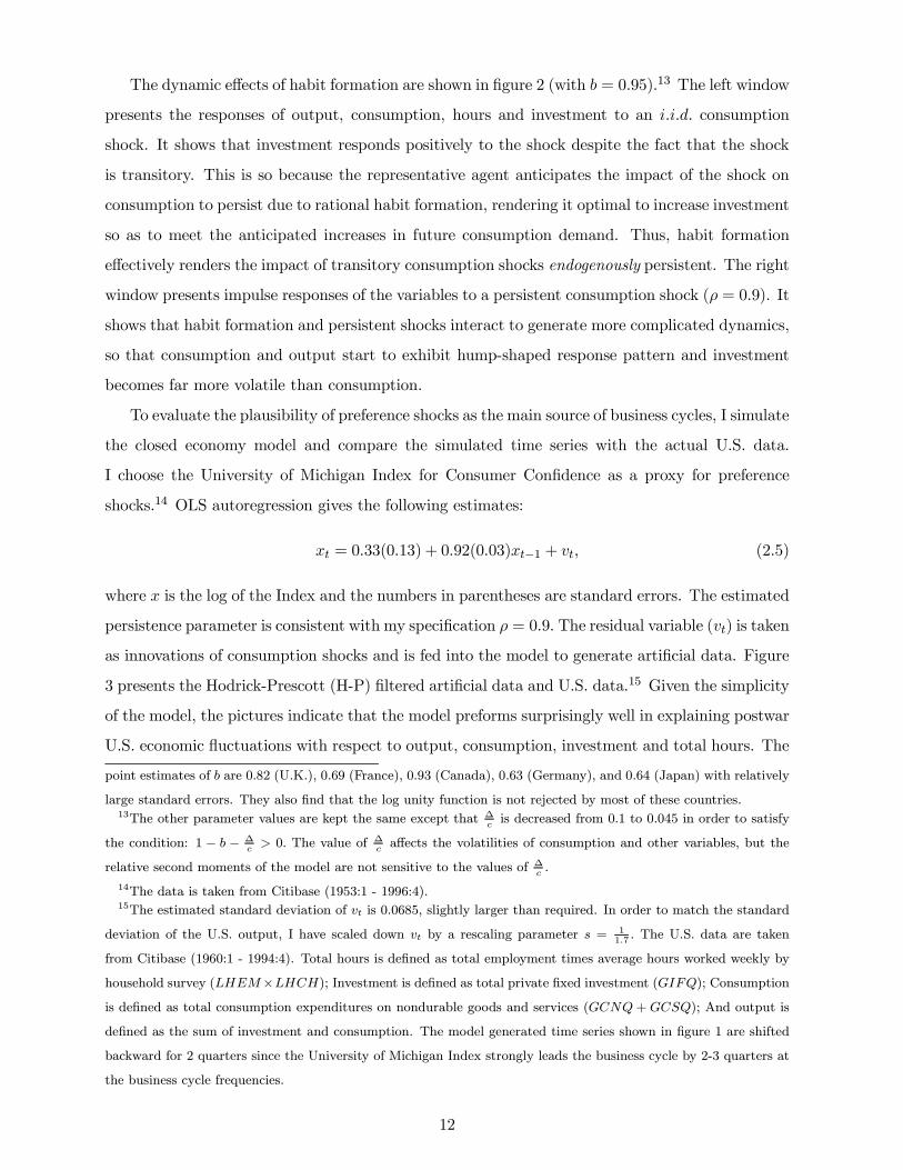
The dynamic e®ects of habit formation are shown in ¯gure 2 (with b = 0:95).13 The left window

presents the responses of output, consumption, hours and investment to an i:i:d: consumption

shock. It shows that investment responds positively to the shock despite the fact that the shock

is transitory. This is so because the representative agent anticipates the impact of the shock on

consumption to persist due to rational habit formation, rendering it optimal to increase investment

so as to meet the anticipated increases in future consumption demand. Thus, habit formation

e®ectively renders the impact of transitory consumption shocks endogenously persistent. The right

window presents impulse responses of the variables to a persistent consumption shock (½ = 0:9). It

shows that habit formation and persistent shocks interact to generate more complicated dynamics,

so that consumption and output start to exhibit hump-shaped response pattern and investment

becomes far more volatile than consumption.

To evaluate the plausibility of preference shocks as the main source of business cycles, I simulate

the closed economy model and compare the simulated time series with the actual U.S. data.

I choose the University of Michigan Index for Consumer Con¯dence as a proxy for preference

shocks.14 OLS autoregression gives the following estimates:

xt = 0:33(0:13) + 0:92(0:03)xt¡1 + vt; (2.5)

where x is the log of the Index and the numbers in parentheses are standard errors. The estimated

persistence parameter is consistent with my speci¯cation ½ = 0:9: The residual variable (vt) is taken

as innovations of consumption shocks and is fed into the model to generate arti¯cial data. Figure

3 presents the Hodrick-Prescott (H-P) ¯ltered arti¯cial data and U.S. data.15 Given the simplicity

of the model, the pictures indicate that the model preforms surprisingly well in explaining postwar

U.S. economic °uctuations with respect to output, consumption, investment and total hours. The

point estimates of b are 0:82 (U.K.), 0:69 (France), 0:93 (Canada), 0:63 (Germany), and 0:64 (Japan) with relatively

large standard errors. They also ¯nd that the log unity function is not rejected by most of these countries.13The other parameter values are kept the same except that ¢

cis decreased from 0:1 to 0:045 in order to satisfy

the condition: 1 ¡ b ¡ ¢c> 0: The value of ¢

ca®ects the volatilities of consumption and other variables, but the

relative second moments of the model are not sensitive to the values of ¢c.

14The data is taken from Citibase (1953:1 - 1996:4).15The estimated standard deviation of vt is 0:0685, slightly larger than required. In order to match the standard

deviation of the U.S. output, I have scaled down vt by a rescaling parameter s =11:7 : The U.S. data are taken

from Citibase (1960:1 - 1994:4). Total hours is de¯ned as total employment times average hours worked weekly by

household survey (LHEM£LHCH); Investment is de¯ned as total private ¯xed investment (GIFQ); Consumptionis de¯ned as total consumption expenditures on nondurable goods and services (GCNQ+GCSQ); And output is

de¯ned as the sum of investment and consumption. The model generated time series shown in ¯gure 1 are shifted

backward for 2 quarters since the University of Michigan Index strongly leads the business cycle by 2-3 quarters at

the business cycle frequencies.

12

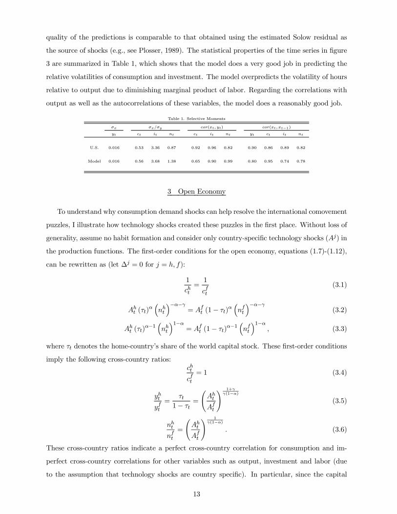
quality of the predictions is comparable to that obtained using the estimated Solow residual as

the source of shocks (e.g., see Plosser, 1989). The statistical properties of the time series in ¯gure

3 are summarized in Table 1, which shows that the model does a very good job in predicting the

relative volatilities of consumption and investment. The model overpredicts the volatility of hours

relative to output due to diminishing marginal product of labor. Regarding the correlations with

output as well as the autocorrelations of these variables, the model does a reasonably good job.

Table 1. Selective Moments

¾x ¾x=¾y cor(xt; yt) cor(xt; xt¡1)yt ct it nt ct it nt yt ct it nt

U.S. 0.016 0.53 3.36 0.87 0.92 0.96 0.82 0.90 0.86 0.89 0.82

Model 0.016 0.56 3.68 1.38 0.65 0.90 0.99 0.80 0.95 0.74 0.78

3 Open Economy

To understand why consumption demand shocks can help resolve the international comovement

puzzles, I illustrate how technology shocks created these puzzles in the ¯rst place. Without loss of

generality, assume no habit formation and consider only country-speci¯c technology shocks (Aj) in

the production functions. The ¯rst-order conditions for the open economy, equations (1.7)-(1.12),

can be rewritten as (let ¢j = 0 for j = h; f):

1

cht=1

cft(3.1)

Aht (¿t)®³nht

´¡®¡°= Aft (1¡ ¿t)®

³nft

´¡®¡°(3.2)

Aht (¿t)®¡1

³nht

´1¡®= Aft (1¡ ¿t)®¡1

³nft

´1¡®; (3.3)

where ¿t denotes the home-country's share of the world capital stock. These ¯rst-order conditions

imply the following cross-country ratios:cht

cft= 1 (3.4)

yht

yft=

¿t1¡ ¿t =

ÃAht

Aft

! 1+°°(1¡®)

(3.5)

nht

nft=

ÃAht

Aft

! 1°(1¡®)

: (3.6)

These cross-country ratios indicate a perfect cross-country correlation for consumption and im-

perfect cross-country correlations for other variables such as output, investment and labor (due

to the assumption that technology shocks are country speci¯c). In particular, since the capital

13

share ¿t is completely dictated by technology ratios across countries, the predicted cross-country

correlations for output, investment and labor are all negative under country speci¯c technology

shocks.16

Consider a positive technology shock in the home country. Consumption increases both at

home and abroad because of an international income e®ect supported by the channel of transfer

of consumption goods. Employment increases at home and decreases abroad for two reasons. The

¯rst is an international substitution e®ect of leisure supported by risk sharing, which causes the

high-productivity country to decrease leisure and the low-productivity country to increase leisure.

This substitution e®ect exists regardless of capital mobility, as long as countries can trade in

currently produced goods. The second is capital mobility, which permits existing capital to °ow

to the highest returns, thus increasing demand for labor at home and decreasing labor demand

abroad. Consequently, cross-country correlations for employment (as well as output) are negative.

Investment increases at home and decreases in the foreign country also for two reasons. Firstly,

the ability to transfer investment goods across national borders induce national savings °ow to

the highest expected returns; Secondly, capital mobility implies that the direct foreign investment

is positive in the home country and negative in the foreign country (capital drain). Hence, general

equilibrium theory predicts that cross-country correlations for output, employment and investment

are all negative under technology shocks unless these shocks are highly positively correlated across

countries.

Thus puzzles arise: the predicted cross-country correlations are much higher for consumption

than for output, while in the data the opposite is true; and the predicted cross-country correlations

of employment and investment are negative, while in the data they are positive. Furthermore, the

predicted volatilities for both investment and net exports relative to output are excessively large

16The cross-country ratios indicate that the volatilities of the model are very sensitive to the inverse labor supply

elasticity parameter °. As ° approaches zero, for example, even a very small technology shock can generate extremely

volatile movements in output and labor due to factor mobility across countries. The volatility of factor mobility can

be determined by log-linearizing equation (3.5), which givesµ1

1¡ ¿¶¿t =

1 + °

°a(1¡ ®)³Aht ¡ Aft

´;

where circum°ex variables denote percentage changes around the steady state. Assuming that country speci¯c

technology shocks have identical variances (¾2A) and are uncorrelated, we have

¾¿ =p2(1¡ ¿ ) 1 + °

°(1¡ ®)¾A:

For example, let the steady-state value of the world capital share ¿ = 0:5, and let ° = 0:25 and ® = 0:3; we then

have ¾¿ ¼ 5¾A: It is also clear that ¾¿ approaches in¯nity as ° approaches zero.

14

compared to the observed values.17 There has been no shortage of explanations in the literature

for these puzzles, with most of them focusing on market frictions and market incompleteness that

inhibit international risk sharing. The problem is that some of these puzzles, especially the cross-

country consumption correlations puzzle, are extremely robust to model modi¯cations such that

none of the explanations advanced to date in the literature can completely resolve these puzzles

at once.

There is no puzzle, however, if the primary source of shocks causing short-run economic °uc-

tuations in international trade comes from the demand side (consumption) rather than from the

supply side (technology). Under consumption demand shocks, the ¯rst-order conditions for the

open economy implies the following cross-country ratios:

cht ¡¢htcft ¡¢ft

= 1; (3.7)

17To see this, consider the percentage changes in the home-country's quantities relative to the steady state.

Log-linearizing equation (3.5) and the de¯nition of national investment around the steady state and simplifying

gives:

yht ¡ yft = 1

1¡ ¿ ¿t

{t =1

±Kt+1 ¡ 1¡ ±

±

³Kt ¡ ¿t

´= It +

1

±¿t;

where I denotes the percentage changes in total world investment. Denote ¾x as the standard deviation for x and

½(x1; x2) as the correlation between x1 and x2. The ¯rst equation implies:

¾2yh + ¾2yf ¡ 2½(yh; yf )¾yh¾yf = 4¾2¿ :

Suppose county-speci¯c technology shocks are symmetric and are uncorrelated, then we can have the approximations,

¾2yh = ¾2yf and ½(y

h; yf ) · 0: Hence, 2¾2yh · 4¾2¿ ; which implies ¾yh ·p2¾¿ :

On the other hand, the investment equation implies

¾2i = ¾2I +

µ1

±

¶2¾2¿ + 2½(I; ¿)¾I¾¿ :

Given that the quarterly rate of capital depreciation ± = 0:025; we have¡1±

¢2= 160: Hence the variance of i is clearly

dominated by the variance of ¿ , which gives the approximation ¾i ¼ 40¾¿ . These results imply that ¾i ' 28¾y;

namely, investment is at least 28 times more volatile than output under country-speci¯c technology shocks. In the

data, however, investment is only about as 3 times volatile as output. Such an extremely volatile investment leads

also to an extremely volatile net exports. To see this, note that the percentage changes in net exports are given by

cnxt = yt ¡ scct ¡ si{t;where sc + si = 1 are the steady-state shares of consumption and investment in output. Clearly the volatility of

net exports is dominated by that of investment, hence we have ¾2nx ¼ s2i¾2i (consumption is much less volatile thanoutput due to consumption smoothing and risk sharing under income shocks). Assuming that investment share

si = 0:2; we have ¾nx ¼ 0:2¾i ' 5:6¾y; namely, net exports is at least about 6 times more volatile than output. Inthe data, however, net exports is less volatile than output.

15

yht

yft=nht

nft= 1; (3.8)

¿t1¡ ¿t = 1: (3.9)

The last equation implies that the optimal foreign direct investment (capital mobility) is zero (i.e.,

¿t is constant).18 Hence,

iht

ift= 1: (3.10)

These cross-country ratios imply that output, investment and labor are perfectly synchronized

across countries while consumption is imperfectly correlated across countries (due to country-

speci¯c demand shocks). Thus, unless consumption shocks are perfectly correlated across coun-

tries, the predicted cross-country correlations are higher for output than for consumption (as ob-

served in the data); and the predicted cross-country correlations for employment and investment

are positive (as observed in the data).

The intuition is simple. It is a typical story of aggregate demand. Consider an increase in

consumption demand in the home country due to a high urgency to consume. This raises demand

for both domestic output and foreign output under international risk sharing. Hence production

increases both at home and abroad in response to the higher world demand. In the mean time,

investment may also rise both at home and abroad if the increase in demand is persistent, so

that each country can build up more production capacities to sustain the persistent increases

in world demand.19 The higher investment demand across countries reinforces the initial rise in

total world demand. Consequently, we observe strongly positive movements in output, investment

and employment in both countries (perfect correlations). On the other hand, if the urge to

consume (demand shock) is country speci¯c, consumption will be less correlated across countries

than output.20 Furthermore, since capital does not °ow across borders, national savings arise

due mainly to the increases in national investment demand, hence the predicted domestic saving-

investment correlations are positive, as they are in the data.21 In addition, given that ¿t does

not respond to ¢t, the predicted volatilities of investment and net exports are substantially lower

18The reason for ¿t being constant under demand shocks is that domestic investment possibilities o®er su±cient

scope for self-insurance through intertemporal domestic reallocations when the two countries have identical tech-

nologies. Hence foreign direct investment is not optimal unless there are technology shocks which create di®erentials

in returns to capital across countries.19The increases in world demand are persistent either due to persistent demand shocks or due to habit formation

in consumption.

20Risk sharing maximizes the cross-country correlations for (ct ¡¢t) ; not for ct.21Under symmetric consumption demand shocks across countries, net exports of newly produced goods can be

either positive or native (with zero mean) and is not closely correlated with world investment (which is always

16

than they are under technology shocks.22

Thus, general equilibrium theory predicts that when urges to consume arise in a speci¯c coun-

try, international risk sharing causes a world-wide production synchronization, giving rise to the

apparently puzzling phenomenon that \When an economic boom produces high output, employ-

ment, and investment in the United States, there is usually a simultaneous boom in other indus-

trialized countries." (Baxter and Farr, 2001). This phenomenon is puzzling, however, only if we

assume that international business cycles are driven primarily by technological di®erentials across

countries. With consumption demand shocks as the main driving force of business cycles, the afore-

mentioned phenomenon is expected and all the international comovements \puzzles" disappear at

once.

The above discussions can be quanti¯ed by impulse response analysis. Let the capital-income

share ® = 0:3; the time-discount factor ¯ = 0:99; the labor supply elasticity parameter ° = 0,

the capital depreciation rate ± = 0:025; the steady state habit-demand to consumption ratio

¢c = 0:045; and the habit formation parameter b = 0:95: Figure 4 shows the impulse responses of

output, consumption, hours and investment (1 = home country and 2 = foreign country) to an i:i:d:

technology shock at home. It is seen there that output, investment and employment increase in

the home country and decrease in the foreign country in response to the shock at home, indicating

negative cross-country correlations for these variables. In the meantime consumption increases

in both countries and shows perfect correlations across countries. Highly persistent technology

shocks give qualitatively similar results.

The dynamic e®ects of consumption shocks are dramatically di®erent. Figure 5 shows the

impulse responses of the same variables to an i:i:d: consumption demand shock at home. It is

seen there (1 = home country and 2 = foreign country) that movements of output, investment

and employment are not only highly persistent in each country but also highly correlated across

countries, indicating the \demand-pull" cross-country e®ects of consumption shocks. It shows

positive). Hence,

Cov(sj ; ij) = Cov(nxj + I; I) = ¾2I ;

and

¾2s = ¾2nx + ¾

2I ;

for j = h; f: These imply

½(sj ; ij) =¾I¾s=

¾Ip¾2nx + ¾

2I

2 (0; 1):

It is clear then that the saving-investment correlation is not only positive but also close to one since the volatility

of net exports is small relative to that of investment under persistent consumption shocks.22When ¿t is constant, the volatility of investment for each country becomes the same as that of the aggregate

world investment.

17

how an economic boom in one country can lead to a simultaneous boom in another country

(production synchronization). It also shows that consumption movements are less synchronized

across countries due to the shock being country speci¯c.

It is worth noting that the endogenous propagation mechanism created by habit formation in

one country can induce similar propagation mechanism in another country through the \demand-

pull" channel of business cycle transmissions, even if the other country does not have endogenous

propagation mechanisms. For example, let the habit formation parameter in the foreign country

be zero (bf = 0): Then a negative i:i:d: consumption shock in the foreign country generates only

a temporary drop in output in that country. However, a negative i:i:d: consumption shock in the

home country can lead to a prolonged recession in the foreign country because the endogenous

propagation mechanism in the home country generates persistently lower consumption demand

for goods produced both at home and abroad (see ¯gure 6). Hence, there is the well-known

phenomenon that the whole world catches cold when the U.S. economy sneezes; And the cold is

never cured before the sneezes are over.23

4 Robustness

Although market frictions are not preconditions for explaining international business cycle

puzzles, they are by no means unrealistic features of actual open economies. This section dis-

cusses whether the predicted consumption-driven business cycles are robust to market frictions.

This discussion also helps understand the acknowledged robustness of the anomalies created by

technology shocks.

There are three types of markets in the one-good model to support international risk sharing:

markets for currently produced consumption goods, markets for currently produced investment

goods and markets for ¯xed assets. The ¯rst two types of markets provides risk sharing via

transfer of consumption goods or future capital goods across borders, and the third type of markets

provides risk sharing via transfer of factors of production across borders. The frictions introduced

so far in the literature, whether they be transportation costs (Backus, Kehoe and Kydland, 1992),

nontraded goods (Stockman and Tesar, 1995), or incomplete ¯nancial markets (Baxter and Crucini,

1995; Kollmann, 1996; and Kehoe and Perri, 2000), all amount to inhibiting transactions in the

23This raises a knotty identi¯cation problem for the nature of shocks using national data, as any apparent serial

correlations and highly persistent movements in national data, suggesting a source of permanent shocks in that

nation, could be driven entirely by neighboring countries' transitory shocks. The converse is also true; Namely, the

lack of serial correlations in national data does not imply the lack of endogenous propagation mechanisms if the

main source of shocks comes from a foreign country which lacks endogenous propagation mechanisms.

18

three types of markets in one way or another.

A. Frictions in Asset markets

Consider ¯rst frictions in the capital-good market. Assume that there exists a transport cost

associated with shipping ¯xed capital across the border with the cost function,

µ

2(¿t ¡ ¿)2Kt;

so that the marginal transport cost is proportional to foreign direct investment.24 Assume that

the transport cost is shared equally by the two countries. The resource constraint, equation (1.5),

becomes Xj

cjt + [Kt+1 ¡ (1¡ ±)Kt] ·Xj

³¿ jtKt

´® ³nht

´1¡® ¡ µ2(¿t ¡ ¿)2Kt: (4.1)

It is clear that the transport cost has no e®ects under consumption shocks (since the optimal

value of ¿t is constant under demand shocks). It is nevertheless worthwhile to discuss why the cost

also o®ers little help in resolving the international business cycle \puzzles" created by technology

shocks. To sharpen the analysis, consider the extreme case where the transport cost parameter

µ is in¯nity so that capital mobility is eliminated entirely in every period (i.e., ¿t = ¿ for all t).

With ¿t ¯xed, the ¯rst-order conditions for the open economy with technology shocks, equations

(3.1) and (3.2), imply the following cross-country ratios:

cht

cft= 1; (4.2)

nht

nft=

ÃAht

Aft

! 1®+°

; (4.3)

yht

yft=

ÃAht

Aft

! 1+°®+°

: (4.4)

These ratios are very similar to those of the complete-market economy (3.4)-(3.6). Thus, open

economies with incomplete asset markets behave qualitatively the same as open economies with

complete markets: Under technology shocks, the cross country correlations remain higher for con-

sumption than for output, and the cross-country correlations for output and employment remain

negative.25

24An alternative restriction is that ¿t must be determined one period in advance. Under this restriction, ¿t cannot

respond to technology shocks in time period t but ¿t+1 will respond if the shocks are expected to be persistent.25Baxter and Crucini (1995) consider a model in which agents are restricted to trade only goods and noncontingent

real debt. Since the channel for international transfer of currently produced goods is kept intact, their model is

similar to models with adjustment costs in ¿t.

19

The intuition is as follows. International risk sharing under technology shocks gives rise to both

a cross-country income e®ect on consumption and a cross-country substitution e®ect on leisure.

The income e®ect leads to higher consumption across countries (via transfers of consumption goods

from a more productive country to a less productive country). The substitution e®ect leads to

higher economic activity in the more productive country and lower activity in the less productive

country (so that countries enjoy less leisure when productivity is high and more leisure when

productivity is low, implying negative correlations for employment across countries). Capital

immobility dampen but does not undo these two e®ects. Consequently, the structure of asset

markets does not resolve the puzzles created by technology shocks.

Risk sharing under preference shocks, on the other hand, gives rise to a di®erent substitution

e®ect of leisure. It works through consumption-good transfers from the less urgent country to

the more urgent country, leading to higher consumption demand in both countries. Consequently,

both countries opt to enjoy less leisure when world demand is high and more leisure when world

demand is low, rendering production activities highly synchronized across countries. Since there

is no technology di®erentials involved, this mechanism does not generate unbalanced demand for

capital goods across countries. Consequently, the structure of asset markets is irrelevant under

consumption shocks.26

The only signi¯cant di®erence the absence of capital mobility makes under technology shocks is

that the elasticities of the cross-country ratios with respect to cross-country technology di®erentials

are reduced, hence the volatility of economic activities is smaller. In particular, the volatilities

of investment and net exports relative to output are substantially lowered due to the absence of

foreign direct investment.27

Table 2 reports the quantitative e®ects of the transport cost on volatilities of investment and net

exports under technology shocks. It shows that the excess volatility of investment and the excess

volatility of net exports go hand in hand - all are driven by the technology-induced international

capital movements (foreign direct investment) in the model. In order for the predicted relative

volatility ratio of net export and output to be less than one (or for investment volatility to be

26Cross-country capital movements will be observed under consumption shocks, however, if the production tech-

nologies di®er across countries. In this case, the structure of asset markets or capital adjustment costs can be

e®ective in reducing international capital mobility under consumption shocks. For analysis on capital movements

in a deterministic two-country model with di®erent production technologies, see Wan (1971).27The elasticities measure how sensitive international comovements are to technology shocks. For example, com-

paring equations (4.3)-(4.4) with equations (3.5)-(3.6), the elasticity of cross-country output ratio with respect to

cross-country technology ratio is reduced from 1+°°(1¡®) to

1+°°+® . Suppose ° = 0:25; ® = 0:3; then the reduction in

aggregate volatilities in the model due to incomplete asset markets is more than 3 times.

20

roughly consistent with the data), µ has to be greater than one; Namely, the marginal cost of

shipping ¯xed capital across the border, µ (¿t ¡ ¿)Kt, has to be greater than the total value offoreign direct investment.

Table 2. Relative Volatilities of Investment and Net Exports (At)

U.S. Data µ = 0 µ = 0:1 µ = 0:5 µ = 1 µ = 2 µ = 10

¾i=¾y 3.36 39.5 22.4 8.27 4.88 3.10 2.12

¾nx=y=¾y 0.25a » 0.86a 8.44 4.79 1.77 1.04 0.66 0.46

a : Reported by Backus, Kehoe and Kydland (1992).

B. Frictions in Currently-Produced Goods Markets

The above discussion suggests that the most e®ective restrictions to reduce cross-country cor-

relations for consumption and to increase cross-country correlations for output under technology

shocks must involve frictions in the currently-produced goods markets. To avoid autarky, obvi-

ously, the possibility of trade for certain goods is needed. To ensure maximum possible cross-

country correlation for output and minimum possible cross-country correlation for consumption

under technology shocks (so as to best resolve the international comovements puzzles), assume

that international borrowing for ¯xed assets and consumption goods are both prohibited, but bor-

rowing for investment goods are possible. Furthermore, assume that real debt contracts can be

written in a way such that investment in each country are perfectly synchronized. This amounts

to maximize cross country correlations for national income (output) under technology shocks.28

Under these restrictions, capital is essentially \public" (shared with ¯xed proportions), and each

country is forced to absorb its own output by domestic consumption and \public" investment:

cjt + ¼jIt = y

jt ; j = h; f ;

for all t.

Due to the restrictions, the income e®ect of technology shocks can no longer take place in the

form of transfer of consumption goods, rendering cross-country synchronization for consumption

extremely di±cult. On the other hand, the income e®ect can take place in the form of production

activities, rendering cross-country synchronization for output possible. To see why, note that cross-

country synchronization for consumption (risk sharing) is still the ultimate goal of the planner

(representative world agent) under technology shocks. But the absence of markets for transfer

28These assumptions do not mean to be realistic. The point is to show how far one has to go in order to resolve

the international comovements \puzzles" created by the technology shocks. It is therefore not important to specify

the exact underling market structure giving rise to such risk-sharing arrangements.

21

of consumption goods forces the planner to achieve this goal by synchronizing productions across

countries (so as to increase cross-country correlations for consumption). Thus, international risk

sharing in the current context amounts essentially to maximize cross-country correlations for

consumption subject to the constraints:

cjt = yjt ¡ ¼jIt; (4.5)

for j = h; f . Hence we have

Cov(ch; cf ) = Cov³yh ¡ ¼I; yf ¡ (1¡ ¼)I

´= Cov(yh; yf ) + ¼(1¡ ¼)¾2I ¡ ¼Cov(yf ; I)¡ (1¡ ¼)Cov(yh; I):

Using the fact that the two countries are symmetric and identical, we can simplify the equation

as

½(ch; cf )¾2c = ½(yh; yf )¾2y +

1

4¾2I ¡ ½(yj; I)¾y¾I :

Given that©½(yh; yf ); ½(yj ; I)

ªare all nonnegative in the current context, so clearly ½(ch; cf ) is

maximized when ½(yh; yf ) is maximized. Hence, ½(ch; cf ) < ½(yh; yf ) is possible provided that

½(yj; I) is large enough. Then the cross-country consumption-output correlation puzzle can be

resolved.

However, risk sharing by production synchronization does not necessarily resolve the problem

of negative cross-country correlation for employment. To see this, consider a scenario in which

national output in the two countries are perfectly synchronized (yht = yft ). This implies

1 =Ah

Af

µnh

nf

¶1¡®;

which implies that cross-country correlation for labor is negative in order to support perfect

production synchronization under technology shocks. Namely, countries with high productivity

opt to use less labor and countries with low productivity opt to use more labor in order to

synchronize national income across countries.

This illustrates just how di±cult it is to resolve the international comovement puzzles with

market frictions. Such di±culties do not arise under consumption shocks, however. With con-

sumption shocks, production synchronization is the only natural mechanism for international risk

sharing. Without technology shocks, synchronization in output automatically implies synchroniza-

tion in labor and vice versa. In the current context, however, the absence of markets for transfer of

consumption goods hinders the consumption-demand-pull channel for production synchronization.

But, risk sharing via investment on public capital creates an investment-demand-pull channel for

22

production synchronization. Consequently, when there is an urge to consume in a speci¯c country,

investment in all countries increase, creating a higher world demand for output in each country.

As a result, cross-country correlations are expected to be higher for output than for consumption

and to be positive for output, employment and investment, despite the severe restrictions imposed

on market transactions.29

C. Numerical Analysis

The above discussions can be con¯rmed by numerical analysis. Table 3 reports means and

standard deviations of sample moments computed from 500 simulations of the world economies of

di®erent types of frictions, with sample length of 100 periods in each simulation. Following the

existing literature, all statistics reported are based on H-P ¯ltered time series. Three types of

economies are simulated, one pertaining to complete markets, the second pertaining to incomplete

asset markets and the third pertaining to the economy with both incomplete asset markets and

incomplete good markets.30

The ¯rst column in table 3 reports the puzzles created by technology shocks. The cross-country

correlations are negative for output, employment and investment and are higher for consumption

than for output. Furthermore, the predicted investment and net exports are excessively volatile.

These puzzles do not exist under consumption demand shocks. Namely, the cross-country corre-

lations are positive for output, employment and investment and are lower for consumption than

for output. Furthermore, the predicted investment and net exports volatilities are consistent with

the data.

The second column in table 3 shows that while the assumption of incomplete asset markets

is quite e®ective in bringing down the excess volatilities of investment and trade balance under

29It is certainly possible to create hypothetical situations in which the predicted cross-country correlations are

inconsistent with data under consumption shocks. But this is not the point. The point is to show that frictions

frequently proposed for explaining the international comovements \puzzles" under technology shocks (including even

the extremely unrealistic assumptions adopted here) can hardly diminish the explanatory power of consumption

shocks for business cycles.30Most parameter values are kept the same as in previous sections. Namely, the time-discount factor ¯ = 0:99;

the capital depreciation rate ± = 0:025; the steady state habit-demand to consumption ratio ¢c= 0:045; the

habit formation parameter b = 0:95; the transport cost parameter is set at in¯nity (¿t is constant for all t): Both

technology shocks and consumption shocks are assumed to be uncorrelated with each other and across countries.

The persistent parameters of these shocks are set at 0:9. The only exception is the inverse labor supply elasticity °.

To avoid singularity under technology shocks, I follow the existing literature by setting the labor supply elasticity

parameter ° = 0:25 under both technology shocks and consumption shocks, which implies steady-state hours worked

as fraction of time endowment ¹n = 0:2.

23

technology shocks, it has little e®ect however on altering the negative cross-country correlations

for output and employment implied by the complete-markets model. Asset market frictions have

no e®ects on the model when the source of shocks is from consumption demand.

The third column in table 3 shows that goods-market frictions are very e®ective in resolv-

ing the consumption-output anomaly created by technology shocks. In particular, the frictions

can substantially reduce the cross-country correlation for consumption and substantially increase

the cross-country correlation for output (due to production synchronization ), so that the pre-

dicted cross-country correlations become much higher for output (0:99) than for consumption

(0:1). But, the cross-country correlation for employment remains negative (¡0:73) under technol-ogy shocks. On the other hand, despite of the severe trading restrictions in both the asset markets

and the goods markets, the predictions of consumption shocks remain consistent with all qualita-

tive features of domestic and international business cycles. Namely, the predicted cross-country

correlations are positive for output, investment and employment, and the correlations are higher

for output (0:59) than for consumption (0:01); Domestic consumption, investment and employ-

ment are all positively correlated with domestic output; And domestic output is less volatile than

domestic investment but more volatile than domestic consumption.31

Table 3. Predicted Open-Economy Business Cycle Moments (std. errors in parentheses)

Complete Market Incomplete Asset Market Incomplete Goods Market

At ¢t At ¢t At ¢t

International comovement

½(yh; yf ) -0.93(0.03) 1.00 -0.49(0.13) same 0.99(0.00) 0.59(0.16)

½(ch; cf ) 1.00 0.002(0.31) 1.00 same 0.10(0.31) 0.01(0.28)

½(ih; if ) -0.99(0.00) 1.00 1.00 same 1.00 1.00

½(nh; nf ) -0.98(0.01) 1.00 -0.82(0.06) same -0.73(0.09) 0.57(0.16)

Domestic Comovement

cor(c; y) 0.01(0.20) 0.45(0.16) 0.003(0.19) same 0.01(0.16) 0.72(0.09)

cor(i; y) 0.99(0.01) 0.87(0.03) 0.50(0.14) same 0.99(0.00) 0.78(0.08)

cor(n; y) 0.99(0.00) 0.99(0.00) 0.95(0.02) same 0.28(0.17) 0.99(0.00)

cor(s; i) 0.99(0.01) 0.84(0.07) 0.50(0.14) same 1.00 1.00

cor(nx=y; y) -0.99(0.01) -0.88(0.05) -0.50(0.14) same -1.00 -1.00

Relative Volatility

¾c=¾y 0.002(0.00) 0.91(0.18) 0.005(0.00) same 0.01(0.00) 0.80(0.11)

¾i=¾y 38.4(1.12) 3.63(0.16) 2.37(0.37) same 4.68(0.01) 3.26(0.37)

¾nx=¾y 7.21(0.24) 0.51(0.13) 0.86(0.08) same 0.00 0.00

Autocorrelation

½(yt; yt¡1) 0.65(0.08) 0.72(0.07) 0.65(0.08) same 0.64(0.08) 0.75(0.07)

Note: The statistics are based on 500 simulations with sample lenth of 100. All series are H-P ¯ltered.

31Note that under technology shocks, consumption is too smooth and is only weakly positively correlated with

output in all cases. This is due to habit formation.

24

5 The Quantitative Importance of Consumption Shocks

A. Calibrating Consumption Shocks

Like technology shocks, preference shocks are unobservable. The existing literature estimate

technology shocks (the Solow residual) using speci¯ed production functions. In a similar spirit,

Baxter and King (1991) and Stockman and Tesar (1995) estimate preference shocks using a mod-

el's ¯rst-order conditions derived from speci¯ed utility functions.32 Since preferences are time-

nonseparable in my model, it is di±cult to use the ¯rst order conditions directly. Instead, I choose

to use the equilibrium decision rules to back-solve (deduce) the unobservable shock variables from

the observable decision variables.33 In particular, the decision rules for output and investment in

the closed-economy model satisfy:0@ yjt

{jt

1A = ¦1cjt¡1 +¦2

0@ kjt

¢jt

1A ; for j = h; f ;

where ¦2 is a 2 £ 2 matrix with full rank.34 Thus, I can invert the equation to solve for the

unobservable shocks and the capital stock by0@ kjt

¢jt

1A = ¦¡12

0@ yjt

{jt

1A¡¦¡12 ¦1cjt¡1:This approach depends on iteration methods to ¯nd consistent values for the persistence parame-

ters ½j¢ so that the estimated shock processes have AR(1) coe±cients that are consistent with the

calibrated values used in computing the coe±cient matrices ¦1 and ¦2.35 Using real GDP, ¯xed

investment and consumption from the U.S. and Europe respectively as the observables,36 I found:

¢USt = 0:80¢USt¡1 + "USt

¢ERt = 0:88¢ERt¡1 + "ERt

32Similarly, Burnside and Eichenbaum (1996) deduce capacity utilization rate using a model's ¯rst-order conditions

relating capacity utilization to the output-capital ratio.

33This approach is proposed by Ingram, Kocherlakota and Savin (1994, 1997).34Due to symmetry, the open economy model involves singularity when this approach is used to back-solve the

two country-speci¯c consumption shocks. Namely, ¦2 does not have full rank when both ¢h and ¢f are included

in the state vector. Hence I choose to use the closed economy model to solve for ¢t for each country separately.35Namely, I start with an initial guess for ½. I then back solve for the shocks and estimate their persistence values

½. I then use the estimated persistence values in a second round of estimation for the shocks, and so on so forth

until the values converge.36All data are from OECD (1972:2 - 1996:2). To be consistent with the models, the variables are logged and their

time trends are removed by OLS regressions.

25

where the estimated correlation between the two residuals is 0:11.37

An alternative approach for estimating consumption demand shocks is to use measures for

consumer sentiment as a proxy for preference shocks. Using the University of Michigan Index

from the U.S. and the Harmonized Consumer Survey from Europe respectively as measures of

consumer con¯dence in a bivariate VAR regression, Guo and Sturzenegger (1998) ¯nd the esti-

mated persistence parameters ranging from 0:9 to 0:5 for the U.S. economy and from 0:7 to 0:5

for Europe with mild spillover e®ects, and the innovations (shocks) are positively correlated with

correlation equal to 0:45. Univariate autoregressions on the other hand reveal higher persistence.

For example, it is about 0:92 with a standard error of 0:03 for the U.S. (see equation 2.5).

These empirical studies suggest that consumption demand shocks may be highly persistent

and positively correlated across countries. I therefore choose ½h = ½f = 0:9 and corr("h; "f ) = 0:3

as my benchmark.38 The other parameters in the model remain the same as before; Namely,

the time-discount factor ¯ = 0:99; the labor supply elasticity parameter ° = 0:25, the capital

depreciation rate ± = 0:025; the steady state habit-demand to consumption ratio ¢c = 0:045; and

the habit formation parameter b = 0:95: Empirical estimates of the size of the transport cost is

not available. I choose two possible values, µ = f0; 1g, in my simulation analysis.

B. The Contribution of Consumption Shocks

Since consumption shocks and technology shocks give exactly opposite predictions for the cross-

country correlations and since the data lie somewhere in between quantitatively, I add technology

shocks in the simulations so as to see how much of a technology shock is needed in the model in

order to bring the cross-country correlations into closer conformity with the data quantitatively.

This provides an informal measure on the relative importance of consumption shocks. Consistent

with Backus, Kehoe and Kydland (1992), I assume that technology shocks in both countries follow

stationary AR(1) processes,

logAjt = 0:9 logAjt¡1 + "

jat;

with cor("Hat; "Fat) = 0.

39

37Baxter and King (1991) obtain an estimate of 0:97 for the persistence parameter of the consumption shocks

using Euler equations in a standard closed-economy RBC model.38Choosing other values for the persistence parameters (e.g., ½h = ½f = 0:8) produces little di®erence in the

results. None of the statistics except the cross-country correlations for consumption is sensitive to corr("h; "f ):

The cross-country correlation for consumption is determined by corr("h; "f ): For example, the point estimate varies

between zero and 0:43 when corr("h; "f ) changes between zero and 0:45.

39The following results are not sensitive to this speci¯cation.

26

Table 4 reports the predicted moments of the model under both technology and consumption

shocks along with the estimated data moments taken from the existing literature.40 Table 4 shows

that regardless of market frictions, the predictions of the model are qualitatively consistent with

the data. In particular, the predicted cross-country correlations are positive for output, investment

and employment; and the correlations are higher for output than for consumption. With regard

to domestic movements, consumption, investment and employment are all positively correlated

with output, and net exports are negatively correlated with output. Consistent with the data, the

predicted correlations between domestic saving rates and investment rates are strongly positive.

Also, domestic output is less volatile than investment but more volatile than consumption and net

exports. Furthermore, output (as well as the other variables) in the model are all strongly serially

correlated.

The relative importance of consumption shocks in explaining the data is found by comparing

the total variance of output in the presence of both shocks and the total variance of output in the

absence of one of the two shocks. The proportionality of the two types of shocks is determined

by holding the standard deviation of consumption shocks constant while increasing the standard

deviation of technology shocks until a point beyond which the predicted cross-country correlations

for output, consumption and investment are no longer in agreement with the data. For example,

in the second column of table 4 (µ = 0) the proportion of technology shocks is given by the

standard deviation ratio between the innovations of the two type of shocks, "At"¢t= 0:002: With

this proportionality between the two type of shocks, the contribution of technology shocks to the

total variance of output is only 1%:When the contribution of technology shocks to the variance of

output is increased to 3% or above by increasing the standard deviation ratio to 0:003 or higher,

the cross-country correlations for investment become zero and even negative (inconsistent with

the data). In the third column of table 4 (µ = 1), the proportion of technology shocks is given by

the standard deviation ratio "At"¢t

= 0:05:With this proportionality, the contribution of technology

40The estimated second moments reported by existing literature vary quite a lot depending on the particular

countries and sample periods selected as well as on the speci¯c de¯nitions of variables adopted. For example, the

estimated cross-country correlations for output range from 0:81 (reported by Baxter and Farr, 2001) to 0:51 (reported

by Kehoe and Perri, 2000) or even much lower (reported by Backus, Kehoe and Kydland, 1992), and the reported

cross-country correlations for consumption range from 0:67 (reported by Baxter and Farr, 2001) to 0:32 (reported by

Kehoe and Perri, 2000) or even negative (reported by Backus, Kehoe and Kydland, 1992). What remain as robust

features of the data, therefore, are not the quantitative but qualitative characteristics of the data; Namely, given

the sample periods and the countries chosen the cross country correlations are positive and signi¯cantly higher for

output than for consumption, and they are positive for hours and investment. Similar caveats apply to statistics

characterizing domestic business cycles.

27

shocks to the total variance of output is 13%: When the contribution of technology shocks to

the variance of output is increased to 20% or above by increasing the standard deviation ratio

to "At"¢t

= 0:07 or higher, the cross-country correlations for investment become zero and negative.

When the adjustment cost is in¯nity (µ = 107), the maximum contribution of technology shocks to

the variance of output is still less than 27% (the maximum standard-deviation ratio is "At"¢t= 0:09),

beyond which the cross-country correlations for output become smaller than that for consumption

(inconsistent with the data).41

This sensitivity analysis suggests that consumption demand shocks are the dominant force be-

hind economic °uctuations. What remains to be explained by general equilibrium theory, however,

is the procyclical labor productivity over the business cycle. This stylized fact about productivity

is what makes the technology-shock view attractive. Under demand shocks only, labor produc-

tivity is countercyclical due to diminishing marginal product of labor. With technology shocks

explaining less than 27% of output variance, the predicted labor productivity in the current model

is not procyclical enough to account for the data. However, labor hoarding, capacity utilization,

externalities or increasing returns to scale may also help explain the procyclical labor productivity.

See Burnside, Eichenbaum and Rebelo (1993) and Benhabib and Wen (2000) for analyses along

these lines.41Choosing other values of the persistence parameters for consumption demand shocks produces little di®erence

in the results. For example, when ½h = ½f = 0:8; with the standard-deviation ratio "At"¢t

= 0:035; the implied

contribution of technology shocks to the total variance of output is 13%:The corresponding point estimates for sample

moments are: ½(yh; yf ) = 0:58; ½(ch; cf ) = 0:29; ½(ih; if ) = 0:21, ½(nh; nf ) = 0:82 for international comovements,

and ¾c=¾y = 0:89; ¾i=¾y = 3:61; ¾nx=¾y = 0:43; corr(s; i) = 0:87; and corr(nx=y; y) = ¡0:92 for domesticmovements. Allowing for higher proportion of technology shocks produces cross-country correlations for investment

and output that are inconsistent with the data.

The standard deviation of the U.S. output is about 0:017. To match this value, the standard deviation required

for innovations of consumption shocks ("¢) in the model with µ = 0 is 0:023, and the required value is 0:022

in the model with µ = 1: These required standard deviations for consumption innovations are reasonable. For

example, the estimated standard deviations of innovations©"h; "f

ªbased on the equilibrium-decision-rule approach

are f0:032; 0:020g : And the estimated standard deviation of consumption innovations based on the University ofMichigan Index (1953:1 - 1996:4) is 0:069: And the estimates obtained by Guo and Sturzenegger (1998) are 0:049

for both the U.S. and Europe. Hence the data suggest that the variance of consumption shocks is high enough to

account for the observed volatilities in aggregate output.

28

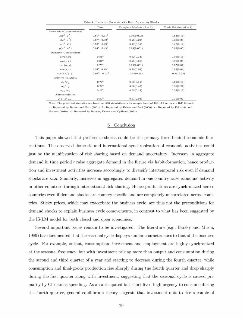
Table 4. Predicted Moments with Both ¢t and At Shocks

Data Complete Markets (µ = 0) Trade Friction (µ = 1)

International comovement

½(yh; yf ) 0.81a, 0.51b 0.99(0.003) 0.63(0.11)

½(ch; cf ) 0.67a, 0.32b 0.26(0.29) 0.30(0.28)

½(ih; if ) 0.73a, 0.29b 0.42(0.15) 0.42(0.14)

½(nh; nf ) 0.84a, 0.43b 0.99(0.001) 0.85(0.05)

Domestic Comovement

cor(c; y) 0.81a 0.52(0.13) 0.46(0.15)

cor(i; y) 0.81a 0.76(0.06) 0.90(0.04)

cor(n; y) 0.78a 0.99(0.001) 0.97(0.01)

cor(s; i) 0.94c, 0.89c 0.79(0.08) 0.93(0.04)

cor(nx=y; y) -0.66d, -0.03d -0.87(0.06) -0.95(0.02)

Relative Volatility

¾c=¾y 0.79b 0.80(0.15) 0.69(0.14)

¾i=¾y 3.24b 4.30(0.46) 3.95(0.27)

¾nx=¾y 0.23a 0.58(0.13) 0.33(0.12)

Autocorrelation

½(yt; yt¡1) 0.89a 0.71(0.08) 0.71(0.07)

Note: The predicted statistics are based on 500 simulations with sample lenth of 100. All series are H-P ¯ltered.

a : Reported by Baxter and Farr (2001). b : Reported by Kehoe and Peri (2000). c : Reported by Feldstein and

Horioka (1980). d : Reported by Backus, Kehoe and Kydland (1992).

6 Conclusion

This paper showed that preference shocks could be the primary force behind economic °uc-

tuations. The observed domestic and international synchronization of economic activities could

just be the manifestation of risk sharing based on demand uncertainty. Increases in aggregate

demand in time period t raise aggregate demand in the future via habit-formation, hence produc-

tion and investment activities increase accordingly to diversify intertemporal risk even if demand

shocks are i:i:d: Similarly, increases in aggregated demand in one country raise economic activity

in other countries through international risk sharing. Hence productions are synchronized across

countries even if demand shocks are country speci¯c and are completely uncorrelated across coun-

tries. Sticky prices, which may exacerbate the business cycle, are thus not the preconditions for

demand shocks to explain business cycle comovements, in contrast to what has been suggested by

the IS-LM model for both closed and open economies,

Several important issues remain to be investigated. The literature (e.g., Barsky and Miron,

1989) has documented that the seasonal cycle displays similar characteristics to that of the business

cycle. For example, output, consumption, investment and employment are highly synchronized

at the seasonal frequency, but with investment raising more than output and consumption during

the second and third quarter of a year and starting to decrease during the fourth quarter, while

consumption and ¯nal-goods production rise sharply during the fourth quarter and drop sharply

during the ¯rst quarter along with investment, suggesting that the seasonal cycle is caused pri-

marily by Christmas spending. As an anticipated but short-lived high urgency to consume during

the fourth quarter, general equilibrium theory suggests that investment opts to rise a couple of

29

quarters earlier before Christmas so as to build up production capacities for the fourth quarter

consumption boom. When the high consumption demand arrives in the fourth quarter, production

and employment increase sharply to meet the urge to consume. If this conjecture is correct, gen-

eral equilibrium theory with preference shifts may provide an uni¯ed explanation for both types of

°uctuations. Another important issue is the policy and welfare implications of stabilization under

preference shocks. When short-run output °uctuations are primarily caused by the urgency to

consume, it may be desirable to smooth real interest rates to accommodate demand for credits,

resulting in a higher output volatility. Consequently, smoothing output over the business cycle

maybe counter-productive and welfare reducing. This may also explain and justify why the U.S.

Fed smooths nominal interest rates over the seasonal cycle. These important issues are beyond

the scope of the paper and are left for future investigation.

7 Appendix 1

A. Proof of Proposition 1

It su±ces to show that Proposition 1 holds near the steady state. Using circum°ex variables to

denote percentage deviations from their steady-state values, the log linearized ¯rst order conditions

for the closed economy without habit formation are given by:

(1¡ !)¢t ¡ !ct = ^t (A)

®nt = ^t + ®kt (B)

^t = Et

h^t+1 ¡ ´kt+1 + ´nt+1

i(C)

±(1¡ s)ct + shkt+1 ¡ (1¡ ±)kt

i= ±®kt + ±(1¡ ®)nt; (D)

¢t = ½¢t¡1 + "t; (E)

where ! > 1 denotes 1=(1¡ ¢¤c¤ ); ´ > 0 denotes (1¡ ®) (1¡ ¯(1¡ ±)) ; and s 2 (0; 1) denotes the

steady state saving ratio. The solutions of the model have the form:0BBBBBBBBB@

kt+1

yt

ct

nt

{t

1CCCCCCCCCA=

0BBBBBBBBB@

¼kk ¼k¢

¼yk ¼y¢

¼ck ¼c¢

¼nk ¼n¢

¼ik ¼i¢

1CCCCCCCCCA0@ kt

¢t

1A :

30

The sign and magnitudes of initial responses of output, consumption, hours, and investment to

a consumption shock are determined by the coe±cients f¼y¢; ¼c¢; ¼n¢; ¼i¢g : Equations (A) and(B) imply

0@ ct

nt

1A =

0@ 0 ¡ 1!

!¡1!

1 1® 0

1A0BBB@kt

^t

¢t

1CCCA : (F)

Substituting out fct; ntg in equations (C)-(E), we obtain

0BBB@kt+1

^t+1

¢t+1

1CCCA =

0BBB@s(1¡±)+±

s ¡± s®¡®¡!+!®s!® (s¡ 1) ±s !¡1!0 ®

®+´ 0

0 0 ½

1CCCA0BBB@kt

^t

¢t

1CCCA+0BBB@0

0

1

1CCCA "t+1: (G)

The 3 eigenvalues of the coe±cient matrix are given byn1¡ ± + ±

s ;®®+´ ; ½

o: Since the steady state

saving ratio is less than one, it is clear that the ¯rst eigenvalue,¡1¡ ± + ±

s

¢> 1 and the other two

eigenvalues are less than one in absolute values, implying that the steady state is a saddle and the

equilibrium of the model is unique.

Decomposing the coe±cient matrix in equation (G) as W = P¤P¡1; where ¤ is a diagonal

matrix with eigenvalues of W as diagonal elements and where P is the corresponding eigenvector

matrix. Arranging the eigenvalues in ascending order in absolute values, it can be shown that

P¡1 =

0BBB@0 0 1

(½s¡s+s±¡±)!± (s! ¡ s¡ ! + 1)0 1 0

1 ± (®+ ´) s®¡®¡!+!®!®(¡s´+±s®+s±´¡±®¡±´)

1(½s¡s+s±¡±)!± (s¡ s! + ! ¡ 1)

1CCCA :Applying the transversality condition on the third equation (solving the system forward), we have

³1 ±(®+´)(®s¡®¡!+!®)

!®(¡s´+±®s+s±´¡±®¡±´)±(1¡s)(!¡1)!(½s¡s+s±¡±)

´0BBB@kt

^t

¢t

1CCCA = 0;

which implies

kt +± (®+ ´) (®s¡ ®¡ ! + !®)

!® (¡s´ + ±®s+ s±´ ¡ ±®¡ ±´)^t +

±(1¡ s)(! ¡ 1)! (½s¡ s+ s± ¡ ±)¢t = 0:

The solution for ¸t is then given by

^t = ¼kt + Á¢t;

where

¼ =!® (s´ ¡ ±®s¡ s±´ + ±®+ ±´)± (®+ ´) (®s¡ ®¡ ! + !®)

31

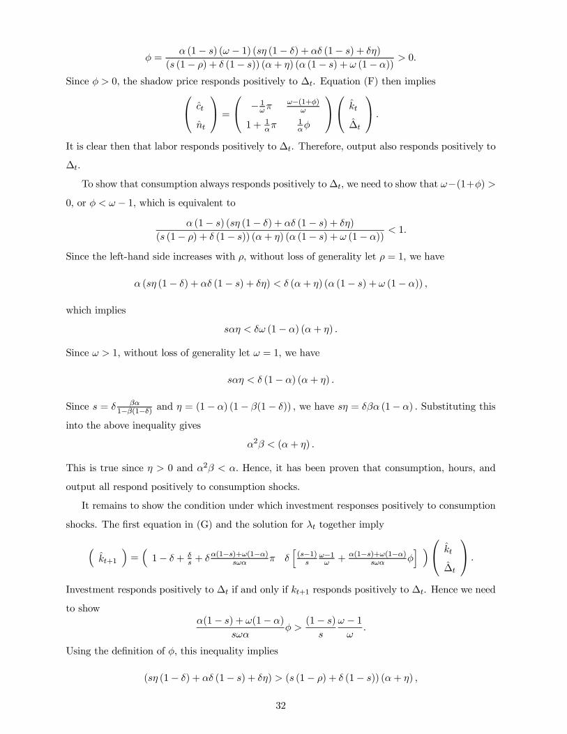
Á =® (1¡ s) (! ¡ 1) (s´ (1¡ ±) + ®± (1¡ s) + ±´)

(s (1¡ ½) + ± (1¡ s)) (®+ ´) (® (1¡ s) + ! (1¡ ®)) > 0:

Since Á > 0; the shadow price responds positively to ¢t. Equation (F) then implies0@ ct

nt

1A =

0@ ¡ 1!¼

!¡(1+Á)!

1 + 1®¼

1®Á

1A0@ kt

¢t

1A :It is clear then that labor responds positively to ¢t. Therefore, output also responds positively to

¢t.

To show that consumption always responds positively to ¢t, we need to show that !¡(1+Á) >0; or Á < ! ¡ 1; which is equivalent to

® (1¡ s) (s´ (1¡ ±) + ®± (1¡ s) + ±´)(s (1¡ ½) + ± (1¡ s)) (®+ ´) (® (1¡ s) + ! (1¡ ®)) < 1:

Since the left-hand side increases with ½, without loss of generality let ½ = 1; we have

® (s´ (1¡ ±) + ®± (1¡ s) + ±´) < ± (®+ ´) (® (1¡ s) + ! (1¡ ®)) ;

which implies

s®´ < ±! (1¡ ®) (®+ ´) :

Since ! > 1; without loss of generality let ! = 1; we have

s®´ < ± (1¡ ®) (®+ ´) :

Since s = ± ¯®1¡¯(1¡±) and ´ = (1¡ ®) (1¡ ¯(1¡ ±)) ; we have s´ = ±¯® (1¡ ®) : Substituting this

into the above inequality gives

®2¯ < (®+ ´) :

This is true since ´ > 0 and ®2¯ < ®: Hence, it has been proven that consumption, hours, and

output all respond positively to consumption shocks.

It remains to show the condition under which investment responses positively to consumption

shocks. The ¯rst equation in (G) and the solution for ¸t together imply

³kt+1

´=³1¡ ± + ±

s + ±®(1¡s)+!(1¡®)

s!® ¼ ±h(s¡1)s

!¡1! + ®(1¡s)+!(1¡®)

s!® Ái ´0@ kt

¢t

1A :Investment responds positively to ¢t if and only if kt+1 responds positively to ¢t. Hence we need

to show®(1¡ s) + !(1¡ ®)

s!®Á >

(1¡ s)s

! ¡ 1!

:

Using the de¯nition of Á, this inequality implies

(s´ (1¡ ±) + ®± (1¡ s) + ±´) > (s (1¡ ½) + ± (1¡ s)) (®+ ´) ;

32

which implies

´ > (1¡ ½) (®+ ´)

or

½ >®

®+ ´=

®

®+ (1¡ ®) (1¡ ¯(1¡ ±)) :

¥

33

References

1. Abel, A., 1990, Asset prices under habit formation and catching up with the Joneses, AmericanEconomic Review v80, n2 (May 1990): 38-42.

2. Backus, D., P. Kehoe and F. Kydland, 1992, International real business cycles, Journal ofPolitical Economy 100, 745-775.

3. Barsky, R. and J. Miron, 1989, The seasonal cycle and the business cycle, Journal of PoliticalEconomy 97, no. 3, 503-534.

4. M. Baxter and R. King, 1991, Productive externalities and business cycles, Institute for Em-pirical Macroeconomics at Federal Reserve Bank of Minneapolis, Discussion Paper 53.

5. Baxter, M and M. Crucini, 1993, Explaining saving-investment correlations, The AmericanEconomic Review 83, no. 3, 416-436.

6. Baxter, M and M. Crucini, 1995, Business cycles and the asset structure of foreign trade,International Economic Review 36, 821-854.

7. Baxter, M. and D. Farr, 2001, Variable capacity utilization and international business cycles,NBER Working Paper no. 8392.

8. Benhabib, J. and Y. Wen, 2000, Indeterminacy, aggregate demand, and the real business cycle,Working Paper, Department of Economics, New York University.

9. Boldrin, M., Christiano, L. and Fisher, J., 2001, Habit persistence, asset returns, and thebusiness cycle, American Economic Review v91, n1 (March 2001): 149-66.

10. Braun, P., Constantinides, G. and Ferson, W., 1993, Time Nonseparability in AggregateConsumption: International Evidence, European Economic Review v37, n5 (June 1993): 897-920.

11. Burnside, C. and Eichenbaum, M., 1996, Factor-Hoarding and the Propagation of Business-Cycle Shocks, American Economic Review v86, n5 (December 1996): 1154-74.

12. Burnside, C., M. Eichenbaum and S. Rebelo, 1993, Labor hoarding and the business cycle,Journal of Political Economy 101 (2), 245-273.

13. Campbell, J. and Cochrane, J, 1999, By Force of Habit: A Consumption-Based Explanationof Aggregate Stock Market Behavior, Journal of Political Economy v107, n2 (April 1999):205-51.

14. Cogley, T. and J. Nason, 1995, Output dynamics in real-business-cycle models, AmericanEconomic Review 85, 492-511.

15. Constantinides, G., 1990, Habit Formation: A Resolution of the Equity Premium Puzzle,Journal of Political Economy v98, n3 (June 1990): 519-43.

16. Deaton, A., 1992, Understanding Consumption, Oxford University Press: New York, NY.

17. Farmer, R. and J. Guo, 1994, Real business cycles and the animal spirits hypothesis, Journalof Economic Theory 63, 42-72.

18. Feldstein, M. and C. Horioka, 1980, Domestic savings and international capital °ows, TheEconomic Journal 90 (June), 314-329.

34

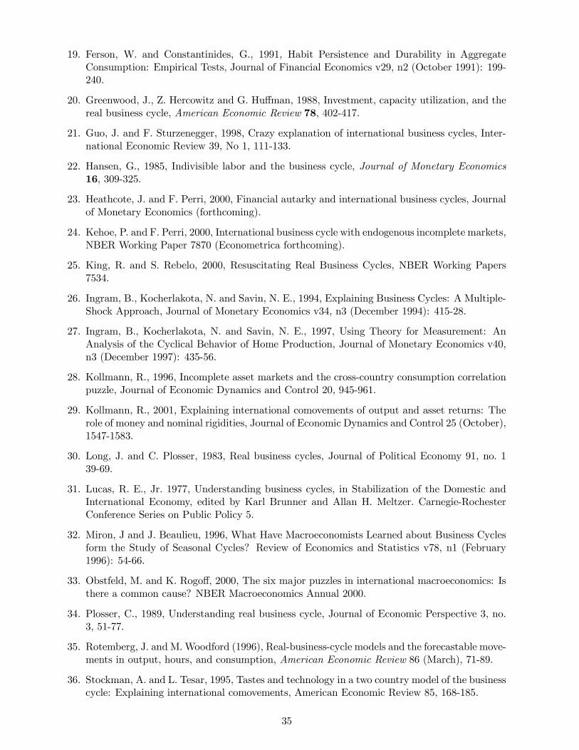
19. Ferson, W. and Constantinides, G., 1991, Habit Persistence and Durability in AggregateConsumption: Empirical Tests, Journal of Financial Economics v29, n2 (October 1991): 199-240.

20. Greenwood, J., Z. Hercowitz and G. Hu®man, 1988, Investment, capacity utilization, and thereal business cycle, American Economic Review 78, 402-417.

21. Guo, J. and F. Sturzenegger, 1998, Crazy explanation of international business cycles, Inter-national Economic Review 39, No 1, 111-133.

22. Hansen, G., 1985, Indivisible labor and the business cycle, Journal of Monetary Economics16, 309-325.

23. Heathcote, J. and F. Perri, 2000, Financial autarky and international business cycles, Journalof Monetary Economics (forthcoming).

24. Kehoe, P. and F. Perri, 2000, International business cycle with endogenous incomplete markets,NBER Working Paper 7870 (Econometrica forthcoming).

25. King, R. and S. Rebelo, 2000, Resuscitating Real Business Cycles, NBER Working Papers7534.

26. Ingram, B., Kocherlakota, N. and Savin, N. E., 1994, Explaining Business Cycles: A Multiple-Shock Approach, Journal of Monetary Economics v34, n3 (December 1994): 415-28.

27. Ingram, B., Kocherlakota, N. and Savin, N. E., 1997, Using Theory for Measurement: AnAnalysis of the Cyclical Behavior of Home Production, Journal of Monetary Economics v40,n3 (December 1997): 435-56.

28. Kollmann, R., 1996, Incomplete asset markets and the cross-country consumption correlationpuzzle, Journal of Economic Dynamics and Control 20, 945-961.

29. Kollmann, R., 2001, Explaining international comovements of output and asset returns: Therole of money and nominal rigidities, Journal of Economic Dynamics and Control 25 (October),1547-1583.

30. Long, J. and C. Plosser, 1983, Real business cycles, Journal of Political Economy 91, no. 139-69.

31. Lucas, R. E., Jr. 1977, Understanding business cycles, in Stabilization of the Domestic andInternational Economy, edited by Karl Brunner and Allan H. Meltzer. Carnegie-RochesterConference Series on Public Policy 5.

32. Miron, J and J. Beaulieu, 1996, What Have Macroeconomists Learned about Business Cyclesform the Study of Seasonal Cycles? Review of Economics and Statistics v78, n1 (February1996): 54-66.

33. Obstfeld, M. and K. Rogo®, 2000, The six major puzzles in international macroeconomics: Isthere a common cause? NBER Macroeconomics Annual 2000.

34. Plosser, C., 1989, Understanding real business cycle, Journal of Economic Perspective 3, no.3, 51-77.

35. Rotemberg, J. andM.Woodford (1996), Real-business-cycle models and the forecastable move-ments in output, hours, and consumption, American Economic Review 86 (March), 71-89.

36. Stockman, A. and L. Tesar, 1995, Tastes and technology in a two country model of the businesscycle: Explaining international comovements, American Economic Review 85, 168-185.

35

37. Wan, H. Y., 1971, A simultaneous variational model for international capital movement, inTrade, Balance of Payments and Growth - papers in international economics in honor ofCharles P. Kindleberger (Edited by J. Bhagwati, R. Jones, R. Mundell and J. Vanek), North-Holland Pub. Co., New York, American Elsevier.

38. Wen, Y., 1998, Capacity utilization under increasing returns to scale, Journal of EconomicTheory 81, 7-36.

36

Figure 1. Impulse Responses to Consumption Shocks without Habit Formation (left window:

½ = 0:9; right window: ½ = 0:98).

37

Figure 2. Impulse Responses to Consumption Shocks with Habit Formation (left window:

½ = 0:0; right window: ½ = 0:9).

38

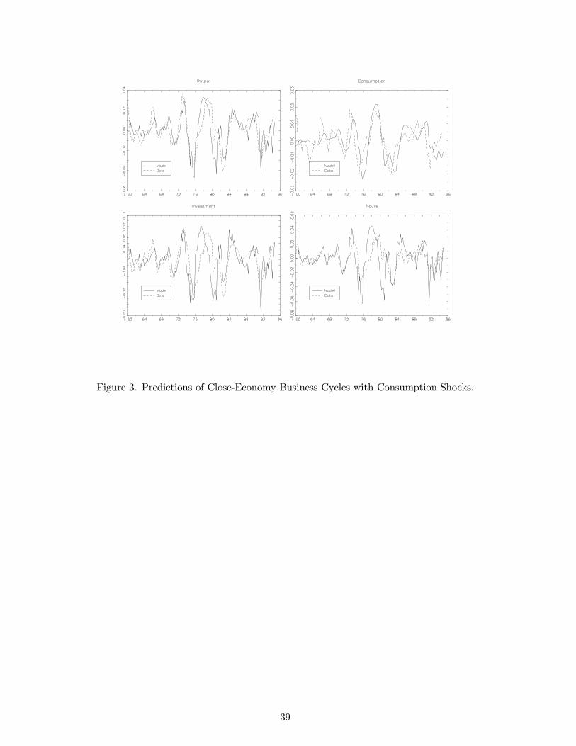
Figure 3. Predictions of Close-Economy Business Cycles with Consumption Shocks.

39

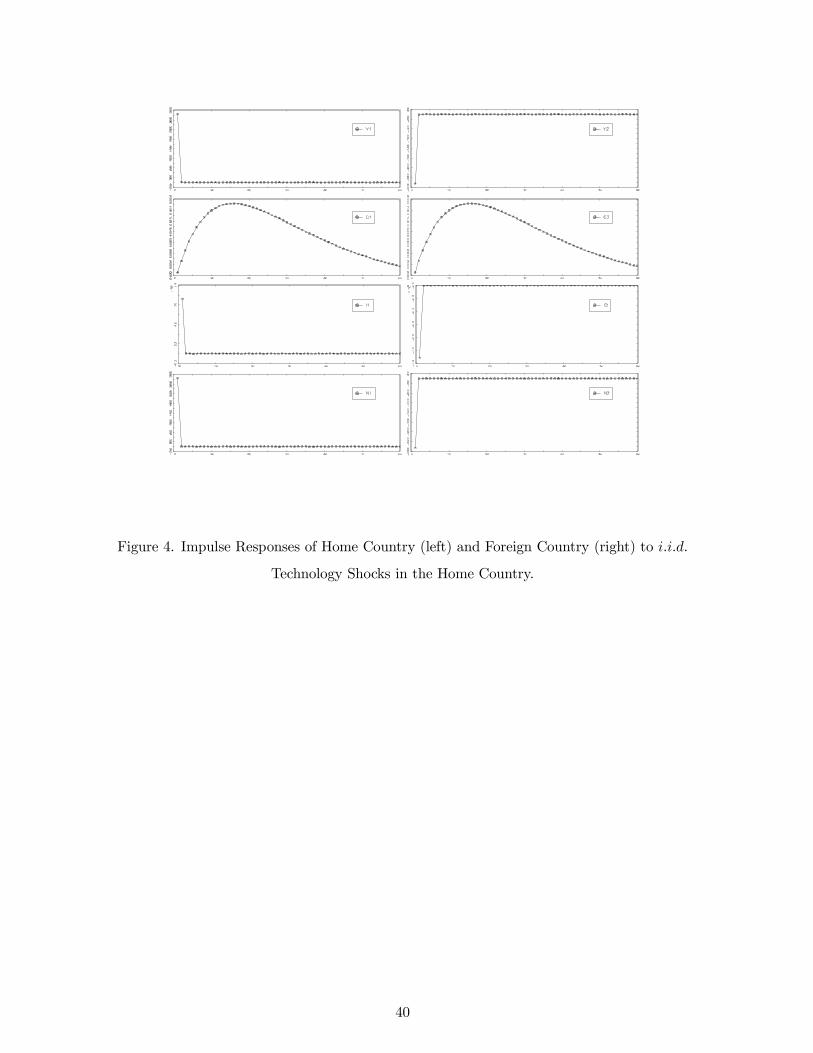
Figure 4. Impulse Responses of Home Country (left) and Foreign Country (right) to i:i:d:

Technology Shocks in the Home Country.

40

Figure 5. Impulse Responses of Home Country (left) and Foreign Country (right) to i:i:d:

Preference Shocks in the Home Country.

41

Figure 6. International Propagation of Business Cycles (i:i:d: shocks).

42