field validation of the environmental conditioning...
TRANSCRIPT

SHRP-A-396
Field Validation of theEnvironmental Conditioning System
Wendy L. AllenRonald L. Terrel
Oregon State University
Strategic Highway Research ProgramNational Research Council
Washington, DC 1994

SHRP-A-396ISBN 0-309-05811-2Product No.: 1024
Program Manager: Edward T. HarriganProject Manager: Rita B. LeahyProgram Area Secretary: Juliet NarsiahProduction Editor: Michael Jahr
May 1994
key words:
asphalt concreteasphalt concrete permeabilityasphalt concrete ruttingbituminous paving mixturesresilient modulus
stripping potentialwater sensitivity
Strategic Highway Research ProgramNational Research Council2101 Constitution Avenue N.W.
Washington, DC 20418
(202) 334-3774
The publication of this report does not necessarily indicate approval or endorsement of the findings, opinions,conclusions, or recommendations either inferred or specifically expressed herein by the National Academy ofSciences, the United States Government, or the American Association of State Highway and TransportationOfficials or its member states.
© 1994 National Academy of Sciences
I 5M/NAP/594

Acknowledgments
The work reported herein has been conducted as a part of project A-003A of the StrategicHighway Research Program (SHRP). SHRP is a unit of the National Research Council thatwas authorized by section 128 of the Surface Transportation and Uniform RelocationAssistance Act of 1987. This project was entitled, "Performance Related Testing andMeasuring of Asphalt-Aggregate Interactions and Mixtures," and was conducted by theInstitute of Transportation Studies, University of California, Berkeley, with Carl L.Monismith as the principal investigator.
The cooperation and efforts of R. Gary Hicks, Teresa Culver, Gail Barnes, Mickey Hines,Oregon State University, and Elf Asphalt are gratefully acknowledged. In addition, theefforts of the transportation authorities of the states of Arizona, California, Georgia,Minnesota, Mississippi, Oregon, and Wisconsin, the province of Alberta, and the WesternFederal Lands Highway Division are acknowledged. Without their cooperation this workcould not have been completed.
.°.
111

Contents
Acknowledgments ................................................. iii
List of Figures ..................................................... ix
List of Tables .................................................... xv
Abstract ........................................................ 1
Executive Summary ................................................ 3
1 Introduction ................................................ 9
Background ........................................... 9Purpose ............................................. 10
2 Experimental Program ........................................ 11
Overview ............................................ 11Selection of Field Sites ................................... 14
Specimen Preparation ..................................... 21
Laboratory Aggregate Preparation ....................... 22Laboratory Asphalt Preparation ......................... 24Laboratory Mixing and Compaction ...................... 40Field Cores ....................................... 44
Specimens Cored from Rutted Beams .................... 47
V

Testing Procedures ...................................... 47
Volumetric Properties ............................... 48MTS Diametral Resilient Modulus ....................... 48MTS Triaxial Resilient Modulus ........................ 49ECS Test ........................................ 50
OSU Wheel Tracking Test ............................ 55Elf Wheel Tracking Test ............................. 59Visual Evaluation of Stripping and Binder Migration .......... 62
3 Results .................................................... 65
ECS Test Program ....................................... 65
ECS Modulus Data ................................. 65
Visual Degree of Stripping and Binder Migration Data ........ 75Permeability Data .................................. 75
OSU Wheel Tracking Program .............................. 77Elf Wheel Tracking Program ............................... 77Field Data ............................................. 78
Weather Data ..................................... 78Traffic Data ...................................... 78
Manual Distress Surveys and Pasco Data .................. 78Field Core Data .................................... 78
4 Discussion and Analysis of Results ............................... 109
ECS Test Results ....................................... 109
ECS Modulus Data ................................ 109
Visual Degree of Stripping and Binder Migration Data ....... 130Permeability Data ................................. 130
OSU Wheel Tracker Results ............................... 133Elf Wheel Tracker Results ................................ 133Field Data ............................................ 139
Weather Data .................................... 139Traffic Data ..................................... 139Field Core Data ................................... 139
Comparison of Test Results ............................... 142
vi

ECS and Field Results .............................. 142ECS and OSU Wheel Tracker ......................... 150ECS and Elf Wheel Tracker .......................... 150
Significance of Findings .................................. 154
5 Guidelines for Specifications .................................... 157
Mixture Properties ...................................... 157ECS Criteria .......................................... 157
Expected Benefits ...................................... 160
6 Conclusions and Recommendations ............................... 163
Conclusions .......................................... 163Recommendations ...................................... 164
7 References ................................................ 165
8 Appendices ................................................ 169
Appendix A: Preparation of Test Specimens of Bituminous Mixturesby Means of the Elf Rolling Wheel Compactor ........ 171
Appendix B: Hamburg Wheel Track Testing of Compacted BituminousMixtures ................................... 177
Appendix C: ECS Test Data .............................. 185
Appendix D: Field Core Data .............................. 191
vii

List of Figures
Figure 2.1 Field validation of water sensitivity, test program ................. 12
Figure 2.2 Water sensitivity field validation sites ......................... 18
Figure 2.3 Specimen identification code ................................ 23
Figure 2.4 Aggregate gradation for Alberta, SPS-5 (AB5) ................... 26
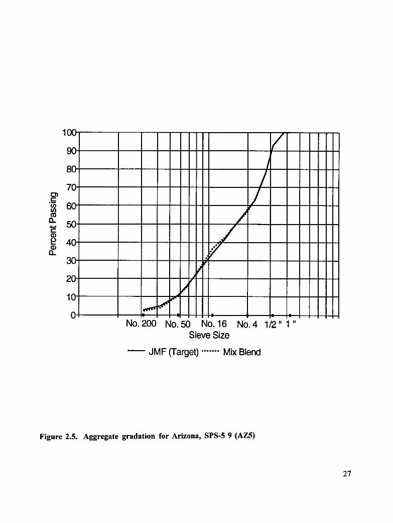
Figure 2.5 Aggregate gradation for Arizona, SPS-5 9 (AZ5) ................. 27
Figure 2.6 Aggregate gradation for California, AAMAS Batch (CAB) ........... 28
Figure 2.7 Aggregate gradation for California, AAMAS Drum (CAD) .......... 29
Figure 2.8 Aggregate gradation for California, GPS-6b (CAG) ................ 30
Figure 2.9 Aggregate gradation for Georgia, AAMAS (GAA) ................ 31
Figure 2.10 Aggregate gradation for Minnesota, SPS-5 (MN5) ................. 32
Figure 2.11 Aggregate gradation for Mississippi, SPS-5 (MS5) ................ 33
Figure 2.12 Aggregate gradation for Rainier, Oregon (OR1) .................. 34
Figure 2.13 Aggregate gradation for Bend-Redmond, Oregon (OR2) ............. 35
Figure 2.14 Aggregate gradation for Mount Baker, Washington (WA1) ........... 36
Figure 2.15 Aggregate gradation for Wisconsin, AAMAS (WAI) ............... 37
Figure 2.16 Schematic of the specimen preparation process ................... 43
ix

Figure 2.17 Schematic of the environmental conditioning system (ECS) .......... 54
Figure 2.18 Schematic of the OSU wheel tracker .......................... 56
Figure 2.19 Measuring positions for rut depth ............................ 60
Figure 2.20 Visual stripping rating chart ................................ 63
Figure 2.21 Binder migration rating chart ............................... 64
Figure 3.1 AB5 ECS results ........................................ 69
Figure 3.2 AZ5 ECS results ........................................ 69
Figure 3.3 CAB ECS results ........................................ 70
Figure 3.4 CAD ECS results ....................................... 70
Figure 3.5 CAG ECS results ....................................... 71
Figure 3.6 GAA ECS results ....................................... 71
Figure 3.7 MN5 ECS results ....................................... 72
Figure 3.8 MS5 ECS results ........................................ 72
Figure 3.9 OR1 ECS results ........................................ 73
Figure 3.10 OR2 ECS results ........................................ 73
Figure 3.11 WA1 ECS results ....................................... 74
Figure 3.12 WIA ECS results ........................................ 74
Figure 3.13 Variation in the coefficient of air permeability with air voids ......... 79
Figure 3.14 Variation in the coefficient of water permeability with air voids ....... 79
Figure 3.15 Variation in the coefficient of water permeability in the ECSprocedure, AB5 ......................................... 80
Figure 3.16 Variation in the coefficient of water permeability in the ECSprocedure, AZ5 ......................................... 80

Figure 3.17 Variation in the coefficient of water permeability in the ECSprocedure, CAB ........................................ 81
Figure 3.18 Variation in the coefficient of water permeability in the ECSprocedure, CAD ........................................ 81
Figure 3.19 Variation in the coefficient of water permeability in the ECSprocedure, CAG ........................................ 82
Figure 3.20 Variation in the coefficient of water permeability in the ECSprocedure, GAA ........................................ 82
Figure 3.21 Variation in the coefficient of water permeability in the ECSprocedure, MN5 ........................................ 83
Figure 3.22 Variation in the coefficient of water permeability in the ECSprocedure, MS5 ......................................... 83
Figure 3.23 Variation in the coefficient of water permeability in the ECSprocedure, OR1 ......................................... 84
Figure 3.24 Variation in the coefficient of water permeability in the ECSprocedure, OR2 ......................................... 84
Figure 3.25 Variation in the coefficient of water permeability in the ECSprocedure, WA1 ........................................ 85
Figure 3.26 Variation in the coefficient of water permeability in the ECSprocedure, WIA ......................................... 85
Figure 3.27 Average rut depths for OSU wheel tracking test program ............ 87
Figure 3.28 Elf wheel tracker results ................................... 90
Figure 3.29 AB5 field cores, diametral modulus data ....................... 97
Figure 3.30 AB5 field cores, triaxial modulus data ......................... 97
Figure 3.31 AZ5 field cores, diametral modulus data ....................... 98
Figure 3.32 AZ5 field cores, triaxial modulus data ......................... 98
Figure 3.33 AZ5 field cores, triaxial modulus data ......................... 99
xi

Figure 3.34 CAB field cores, diametral modulus data ....................... 99
Figure 3.35CAB field cores, triaxial modulus data .......................... 100
Figure 3.36 CAB field cores, triaxial modulus data ........................ 100
Figure 3.37 CAD field cores, diametral modulus data ...................... 101
Figure 3.38 CAD field cores, triaxial modulus data ........................ 101
Figure 3.39 CAD field cores, triaxial modulus data ........................ 102
Figure 3.40 CAG field cores, diametral modulus data ...................... 102
Figure 3.41 GAA field cores, diametral modulus data ...................... 103
Figure 3.42 GAA field cores, triaxial modulus data ....................... 103
Figure 3.43 GAA field cores, triaxial modulus data ....................... 104
Figure 3.44 MN5 field cores, diametral modulus data ...................... 104
Figure 3.45 MN5 field cores, triaxial modulus data ........................ 105
Figure 3.46 MS5 field cores, diametral modulus data ...................... 105
Figure 3.47 OR1 field cores, diametral modulus data ...................... 106
Figure 3.48 OR2 field cores, diametral modulus data ...................... 106
Figure 3.49 WA1 field cores, diametral modulus data ...................... 107
Figure 3.50 WIA field cores, diametral modulus data ...................... 107
Figure 4.1 Slope of mean ECS modulus ratio curves between cycle 1 and cycle 3 117
Figure 4.2 Change in ECS modulus ratio between cycle 1 and cycle 3 ......... 120
Figure 4.3 Change in ECS modulus ratio between cycle 3 and cycle 4 ......... 121
Figure 4.4 Final ECS modulus ratio versus initial ECS modulus .............. 127
Figure 4.5a Final ECS modulus ratio versus initial ECS modulus, by mixture ..... 128
xii

Figure 4.5b Final ECS modulus ratio versus initial ECS modulus, by mixture ..... 128
Figure 4.6a Initial ECS modulus versus air voids, by mixture ................ 129
Figure 4.6b Initial ECS modulus versus air voids, by mixture ................ 129
Figure 4.7 Comparison of ECS and field performance ..................... 148
Figure 4.8 Visual stripping, comparison of field and ECS specimens ........... 149
Figure 4.9 Comparison of ECS and OSU wheel tracker performance .......... 151
Figure 4.10 Comparison of ECS and OSU wheel tracker performanceMN5 and OR2 removed .................................. 152
Figure 4.11 Wheel tracker performance versus ECS performance .............. 153
Figure 5.1 Criteria for the performance of mixtures, OSU wheel trackerversus ECS ........................................... 158
Figure 5.2 Criteria for the performance of mixtures, field versus ECS .......... 159
Figure 5.3 Simple shear criteria .................................... 161
xiii

List of Tables
Table 2.1 Specimen, test procedure and performance modeidentification ........................................... 13
Table 2.2 Field site identification .................................... 16
Table 2.3 Field site location ....................................... 17
Table 2.4 Field sites material identification ............................. 19
Table 2.5 Field site construction information ............................ 20
Table 2.6 Nearest recording weather station ............................ 22
Table 2.7 Aggregate gradations, field section mixtures ..................... 25
Table 2.8 Asphalt and admixture contents .............................. 38
Table 2.9 Asphalt viscosity data and mixing and compactiontemperatures ........................................... 39
Table 2.10 Compaction levels ....................................... 41
Table 2.11 Summary of specimen preparation procedure for rollercompacted slab (SHRP A-003A Task C.5) ...................... 42
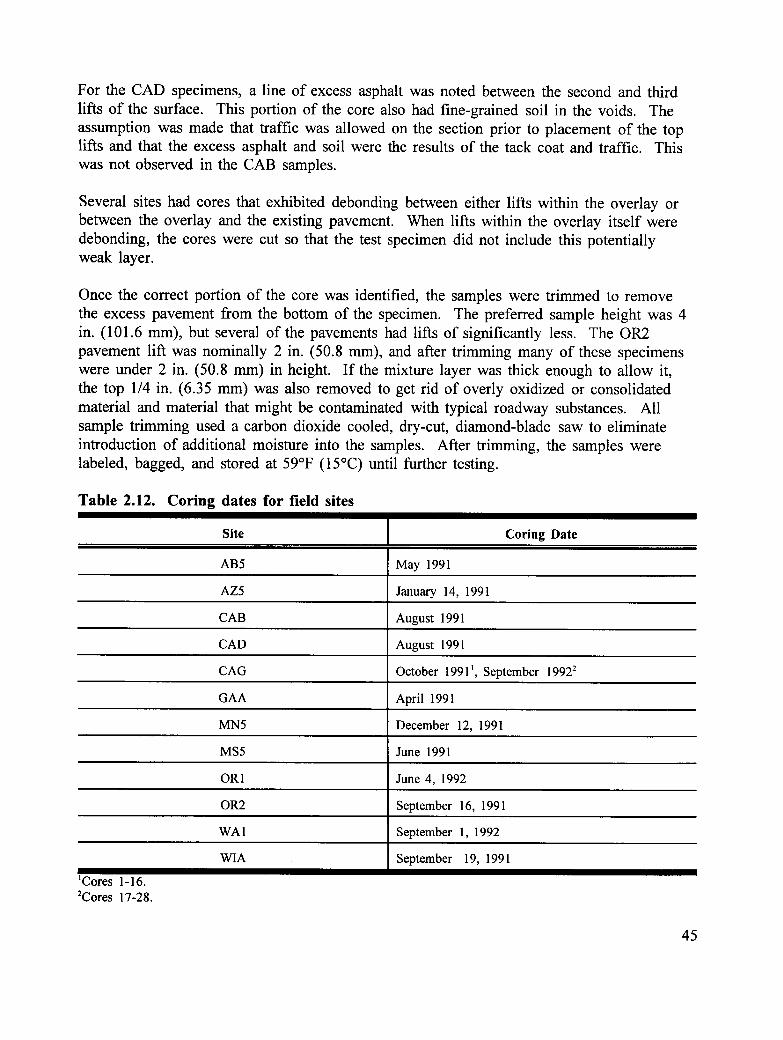
Table 2.12 Coring dates for field sites ................................. 45
Table 2.13 Experiment design for testing of field cores ..................... 46
Table 2.14 Summary of the ECS test procedure .......................... 51
xV

Table 2.15 Experiment design for the ECS testing for SHRP A-003A Task C.5 .... 52
Table 2.16 Summary of OSU wheel tracking test procedure .................. 57
Table 2.17 Experiment design for the OSU wheel tracking for theSHRP A-003A Task C.5 .................................. 58
Table 2.18 Summary of the Elf wheel tracking procedure .................... 61
Table 2.19 Experiment design for the Elf wheel tracker ..................... 61
Table 3.1 ECS test specimens ...................................... 66
Table 3.2 Average coefficients of permeability, intrinsic permeabilities foreach mixture ........................................... 76
Table 3.3 Summary of OSU wheel tracking specimens ..................... 86
Table 3.4 Summary of data from rutted beam cores ....................... 88
Table 3.5 Results of the Elf wheel tracking program ...................... 89
Table 3.6 Monthly total precipitation for the nearest recordingstation, 1990 ........................................... 91
Table 3.7 Monthly normal precipitation for the nearest recording station,30 year average 1961-1990 ................................. 92
Table 3.8 Monthly average temperature for the nearest recordingstation, 1990 ........................................... 93
Table 3.9 Monthly normal temperature for the nearest recordingstation, 30 year average 1961-1990 ........................... 94
Table 3.10 Traffic volumes for the field test sections ....................... 95
Table 3.11 Summary of pavement condition surveys ....................... 96
Table 3.12 Visual stripping evaluation of field cores ...................... 108
Table 4.1 Ranking of mixtures for the ECS test procedure, T intervalsand groupings, entire data set .............................. 111
xvi

Table 4.2 Ranking of mixtures for the ECS test procedure, T intervalsand groupings, freeze data ................................ 112
Table 4.3 Ranking of mixtures for the ECS test procedure,T intervals and groupings, no-freeze data ...................... 113
Table 4.4 Ranking of mixtures for the ECS test procedure, T intervals andgroupings, final ECS modulus ratio, regardless of environmental zone .. 114
Table 4.5 Percent of ECS modulus ratio reduction that occurs in
cycle 1 .............................................. 115
Table 4.6 Mean slope of ECS modulus ratio from cycle 1 to cycle 3 .......... 116
Table 4.7 GLM analysis of the ECS results for mixture type, entire data set ..... 122
Table 4.8 Class variables ........................................ 123
Table 4.9 GLM analysis of ECS results, investigation of significance ofvariable to the model .................................... 124
Table 4.10 GLM analysis of the ECS results model I, entire data set ........... 125
Table 4.11 GLM analysis of the ECS results for model II, entire data set ........ 126
Table 4.12 GLM analysis of the ECS results for freeze versus no-freezeenvironmental zone, final ECS modulus ratios .................. 131
Table 4.13 Ranking of mixtures for the OSU wheel tracking test procedure ...... 134
Table 4.14 GLM analysis of the OSU wheel tracker data ................... 135
Table 4.15 Average air void levels of test specimens, beams and field cores ..... 136
Table 4.16 Mean MTS diametral modulus ratios for rutted beam cores ......... 137
Table 4.17 Performance of mixtures in the Elf wheel tracking test ............ 138
Table 4.18 Deviation of 1990 from 30-year normal, monthly precipitation ....... 140
Table 4.19 Deviation of 1990 from 30-year normal, monthly temperature ....... 141
Table 4.20 Ranking of mixtures for the field cores, based on MTS diametralmodulus ratios ......................................... 143
xvii

Table 4.21 Comparison of ranking of mixtures by test method ............... 144
Table 4.22 GLM analysis of the ECS and field core data by test method ........ 146
Table 4.23 GLM mean modulus ratio values by test method for each mixture .... 147
xviii

Abstract
This research, conducted as part of the SHRP A-003A contract at Oregon State University(OSU), was designed to validate that the Environmental Conditioning System (ECS) candifferentiate among asphalt concrete mixtures that will perform well or poorly in the fieldwith regard to water sensitivity. Twelve test sections were identified, at least two in eachof the four SHRP environmental regions: Wet-Freeze, Dry-Freeze, Wet-No Freeze and Dry-No Freeze. From these 12 sections, specimens were prepared using the original mix design(or mix design as identified by extractions), original aggregates, asphalt and admixtures.Specimens were tested using three procedures: (1) ECS, (2) the OSU wheel tracker, and(3) the Elf asphalt wheel tracker. Cores were taken from the field test sections to evaluateperformance of the mixture in the pavement.
The performance of the mixtures in each of the test procedures was compared in an attemptto develop a correlation among procedures. Results indicate that the ECS test procedurecan distinguish among the relative performance of mixtures, with regard to watersensitivity, as measured in the field and by the OSU and Elf wheel trackers. However, theage of the sections in the field is still relatively young, and water damage is expected tomanifest itself in the future in those pavements identified as water sensitive.

Executive Summary
The work was completed by the A-003A contractor to the Strategic Highway ResearchProgram (SHRP) for Task C.5 on the evaluation of water sensitivity of asphalt concretemixtures. The testing included three phases: (1) laboratory development of procedures andcriteria, (2) validation of the laboratory testing with accelerated laboratory "torture" tests,and (3) field verification of both the laboratory testing program and the acceleratedlaboratory test. This document reports the findings from the third phase, field verification.
The first stage of the A-003A work conducted at Oregon State University (OSU) involvedthe development of the Environmental Conditioning System (ECS), which subjects asphaltmixture specimens to a series of conditioning cycles, including water flow, elevated orlowered temperature, and repeated axial loading (Terrel and AI-Swailmi 1992). Phase twoincluded validation of the ECS procedure with the OSU wheel tracker (French LaboratoireCentral des Pont et Chaussees rutting tester) and the SWK/UN rutting tester, as simulationsof the effect of traffic loading on the mixture (Scholz et. al. 1992). Specimens prepared forthe OSU wheel tracker were water and temperature conditioned in a manner analogous tothat of the ECS procedure.
The final phase of the project involved developed correlations among the ECS, OSU wheeltracker, and the field specimens to verify that ECS can discriminate among differentperformance levels of mixtures in the field, and that the OSU wheel tracker is anappropriate simulation of field conditions. Additional wheel tracking tests were performedby Elf Asphalt in Terre Haute, Indiana, on several of the mixtures. This information isincluded to represent a different type of wheel tracking test apparatus.
The purpose of this portion of the SHRP A-003A program was to demonstrate that the ECStest can accurately discriminate between superior and inferior asphalt concrete mixturesdetermined by their performance in full-scale field test sections. In addition, the correlationamong the performance of mixtures in the ECS, OSU wheel tracker, and field sections wasalso verified. The verification effort differs from the previous work conducted under thisportion of the A-003A project in that all the mixtures used were designed by the localauthority in whose jurisdiction the field section was placed. Other asphalt-aggregatemixtures tested in the SHRP program were prepared according to mix designs developed by

the SHRP A-003A team at the University of California, Berkeley.
This document presents the testing procedures, results, and analysis of data for the twelveasphalt-aggregate mixtures tested in the ECS, OSU wheel tracker, Elf wheel tracker, andfull-scale field test sections. The analysis of data correlates the performance of thesemixtures when subjected to the four types of moisture conditioning inherent in either thetest apparatus or geographical location in which the asphalt mixture was used.
Twelve field sites were selected for the A-003A water sensitivity field validation effort.Sites were selected on the basis of availability of a minimum of 300 lbs. of usable blended
aggregate, 3 gals. (11.4 1) of asphalt cement, required admixtures, mix design information,and cooperation from the presiding authority for field coring. Also, at least two sites wereselected from each of the four SHRP environmental zones. Furthermore, the sites chosenhad to be as old as possible so that there would be several seasons of natural environmentalconditioning in the field.
Forty agencies, including 23 state materials laboratories, the Asphalt Institute and ChicagoTesting Laboratories, the University of Texas, the University of Nevada at Reno and otherswere contacted either by phone or questionnaire to request information on their willingnessto cooperate in the SHRP program and the availability of retained materials. The responseto these questionnaires and related telephone conversations illustrated the lack of retainedmaterials available from most projects.
The testing program for the A-003A field validation of water sensitivity of asphalt concretemixtures involves specimens manufactured by three methods and tested in one or more of
test procedures. Specimens were fabricated using one of the following: a laboratorykneading compactor, a laboratory roller compactor, or field compaction in place at the testsection site. Laboratory-compacted specimens were manufactured at OSU, and field coreswere obtained by the cooperating agencies.
The specimens manufactured at OSU were made from mix designs obtained by SHRP fromthe agency responsible for paving the site. Original aggregate, asphalt and admixtures wereobtained and processed prior to mixing and compacting the specimens. Two mixingprocesses were used to prepare laboratory specimens for the field validation of watersensitivity effort. Individual, 4 in. x 4 in. (101.6 mm x 101.6 mm) specimens were mixedusing protocols developed by the SHRP A-003A study team based upon ASTM D-1561-8l a. Large slabs were mixed using protocols developed for the roller-compacted testspecimens. Eight individual specimens and one large slab were manufactured for 11 of the12 test mixtures. (There was not enough material available from one section forconstruction of OSU wheel tracker beams.) Two OSU wheel tracker beams, 19 in. x 6-1/2in. × 4 in. (482.6 mm x 165.1 mm × 101.6 mm) and eight cores for use in the ECS weresawed from each large slab.
In addition, the governing agency for each site was requested to take cores from the site
4

during the 1990-1991 period as the sites were identified. Eight cores were requested fromeach site, four from the outside wheel path, and four from between the wheel paths.
Each program under SHRP A-003A Task C.5 (ECS, OSU wheel tracking, Elf wheeltracking, and field) employed specimen conditioning in its test procedure, that subjected thespecimen to water damage, followed by measurement of rutting (OSU and Elf wheeltrackers) or reduction in modulus (ECS, rutted beam, and field) and visual evaluation of thedegree of stripping. The performance indicator used for each test procedure was rutting--aratio of conditioned to unconditioned modulus--which develops correlations among test
procedures.
The analysis of the data from the testing program resulted in specifications for the use ofECS in a mix design program. Three levels of mix design are under consideration in theproposed SHRP mix design program (Superpave): level 1, low-traffic-volume roads; level 2,secondary routes, intermediate-traffic-volume roads; and level 3, primary state routes, high-speed and high-volume roads.
As designed in the laboratory, mixtures selected in the preliminary volumetric mix designwill be subjected to short-term oven aging before compaction into specimens for ECS. Thepreliminary mixture design will determine the aggregate and asphalt type to be used,aggregate gradation, and asphalt content. ECS specimens will then be compacted at two airvoid levels: 7 % _+1% for levels 1, 2, and 3, and additional specimens at 10 % + 1% forlevels 2 and 3. These air void levels were chosen in accordance with the pessimum voids
theory proposed by Terrel and A1-Swailmi (1992). Two specimens will be compacted ateach level.
Two specimens of a given mixture and equal air void level will be run through the ECSprocedure, using three or four cycles. The fourth or freeze cycle is optional for use inenvironments that experience freeze-thaw conditions. A plot of the ECS modulus ratioversus cycles will be used to rate the specimen performance.
From the data, a final ECS modulus ratio of 0.7 appears to separate mixtures thatperformed well in ECS, OSU wheel tracker, and the field from those that showeddeterioration in the OSU wheel tracker or the field. It is therefore recommended that the
following procedure be used for Superpave:
Level 1 If the final ECS modulus ratio is < 0.7, the mixture should be treated for moisture
susceptibility and the treated mixture retested in the ECS. If the final ECS modulus ratio isgreater than 0.8, the slope of the curve between cycles 1 and 3 should be investigated. Formixtures with flat slopes, the mixture is expected to perform well, and no treatment isrecommended. For mixtures with steeper slopes, treatment for moisture sensitivity shouldbe considered, because these mixtures may experience moisture damage, though at a slowerrate than those with final ECS modulus ratios of less than 0.7.

Level 2 For the mixture specimens with air void contents of 7 % + 1%, the criterion isthe same as in level two. For the specimens with air voids content of 10 % + 1%, themixture should be treated for moisture susceptibility if the final ECS modulus ratio is < 0.6.Again, the slope of the curve between cycle 1 and cycle 3 is an indicator of continued butdelayed water damage to the mixture.
Level 3 Level 3 varies from level 2 only in the use of additional tests on the specimensafter the ECS test procedure. Simple shear tests will be performed on both conditioned andunconditioned ECS test specimens with a requirement for acceptability of the mixture. Ifthe mixture does not meet the simple shear criteria, it will be redesigned to improve itsperformance. Evaluation of mixtures with the ECS test procedure should eliminate theplacement of mixtures that could experience water damage within the first several years oflife.
The conclusions drawn from the analysis are summarized as follows:
• ECS can discriminate between mixtures that will perform well and those that willperform poorly with regard to water sensitivity of the asphalt mixture.
• The ECS modulus ratio allows for separation of mixtures into performancecategories. Typically, mixtures that have final ECS modulus ratios of greater than0.7 will perform well in the field. Those with lower final ECS ratios should beconsidered for redesign or treatment with admixtures.
• The slope of the modulus ratio curve between cycle 1 and cycle 3 is an indicator ofthe rate of water damage occurring to the specimen. Specimens that have acceptableECS modulus ratios after three cycles may have slopes that indicate potential watersusceptibility problems in the long term.
• Significant change in the modulus ratio occurs in some mixtures between cycle 1and cycle 3, moving them from acceptable to unacceptable or questionable in termsof water sensitivity. The ECS test procedure should not be limited to one cycle.
• Of the variables considered (mixture type, air voids, initial modulus, airpermeability, and water permeability), mixture type, initial modulus, and air voidshave the strongest influence on the final ECS modulus ratio of the mixture.
• The mixtures tested have not been in the field long enough to allow a correlationbetween the cycles of conditioning the ECS and the corresponding period of fieldconditioning.
• The evaluation of visual stripping and migration of asphalt binder in the specimen isextremely subjective.
6

• For new pavements, the increase in resilient modulus caused by long-term aging inthe field may overshadow the reduction in resilient modulus associated with theearly stage of water damage to the pavement mixture.
The following recommendations can be made to further validate the use of the ECSprocedure for determining the water sensitivity of asphalt mixtures:
• A strong correlation between ECS performance and number of years of expectedfield performance has not been made because of the relative youth of the fieldsections. A continued program of coring to further validate and refine the role ofthe ECS test procedure in a mix design program is suggested.
• There should be a controlled program of materials collection, construction of fieldsections, and continued coring to provide a larger data base for ECS criteria.Enough asphalt and aggregate should be sampled at the time of construction to allowmanufacture of both OSU wheel tracker beams (at least four) and ECS specimens.Several of the mixtures tested in the SHRP A-003A program should have beenreplicated because of anomalous results from the OSU wheel tracker. Because of alack of original aggregates, however, there was no opportunity to complete thiswork.
• The procedure for evaluating visual stripping of mixtures should be improved toremove as much of the subjectivity as possible. The use of optical scanners todetermine the amount of stripping in a mixture is worthy of investigation.
• ECS should be used to provide a systematic look at the effects of variations involumetric mixture proportions, such as gradation and asphalt content, on theperformance of mixtures.
• Inclusion of the ECS equipment and procedure per the specification guidelines isrecommended for any mix design system proposed.

1
Introduction
Background
The original proposal by the A-003A contractor to the Strategic Highway Research Program(SHRP) included Task C.5 on the evaluation of water sensitivity of asphalt concretemixtures. The program included a laboratory testing phase for the development andevaluation of procedures and criteria designed to predict the performance of asphalt andaggregate mixtures subjected to water conditioning. A second phase was designed to verifythat the techniques developed in the laboratory phase correlated with the performance ofmixtures subjected to field conditions. An additional component was added to theexperiment when the SHRP staff became concerned about the availability of originalasphalt and aggregate materials and data from in-service field sections for the verificationwork. The extended program completed by the A-003A contractor for the investigation ofwater sensitivity of asphalt concrete mixtures therefore was redesigned to include threephases: (1) laboratory development of procedures and criteria, (2) validation of thelaboratory testing with accelerated laboratory "torture" tests, and (3) field verification ofboth the laboratory testing program and the accelerated laboratory test. This documentincludes the findings from the third phase, field verification.
The first stage of the A-003A work conducted at Oregon State University (OSU) involvedthe development of the Environmental Conditioning System (ECS), which subjects asphaltmixture specimens to a series of conditioning cycles, including water flow, elevated orlowered temperature, and repeated axial loading (Terrel and A1-Swailmi 1992). Phase twoincluded validation of the ECS procedure with the French Laboratoire Central des Ponts etChaussees rutting tester (referred to as the OSU wheel tracker in this report), and theSWK/UN rutting tester, as simulations of the effect of accelerated traffic loading on themixture (Scholz et al. 1992). Specimens prepared for the OSU wheel tracker were waterand temperature conditioned in a manner analogous to that of the ECS procedure.
The final phase of the project involved developing correlations among ECS, OSU wheeltracker, and field specimens to verify that ECS can discriminate among differentperformance levels of mixtures in the field and that the OSU wheel tracker is an
9

appropriate simulation of environmental and traffic-loading conditions in the field.Additional wheel tracking tests were performed by Elf Asphalt in Terre Haute, Indiana, onseveral of the mixtures tested. This information is included to represent the response of adifferent type of wheel tracking test apparatus. Additional information on the watersensitivity of asphalt mixtures may be found in a preliminary literature review conducted byYerrel and Shute (1989).
Purpose
The purpose of this portion of SHRP A-003A was to demonstrate that the ECS test canaccurately discriminate between superior and inferior asphalt concrete mixtures bydemonstrating their performance in full-scale, field test sections. In addition, the correlationamong the performance of mixtures in the ECS, OSU wheel tracker, and field sections wasalso verified. The verification effort differs from the previous work conducted under thisportion of the A-003A project in that all the mixtures used were designed by the localauthority in whose jurisdiction the field section was placed. Other asphalt-aggregatemixtures tested in the SHRP program were prepared according to mix designs developed bythe SHRP A-003A team at the University of California, Berkeley.
This document presents the testing procedures, results, and analysis of data for the 12asphalt-aggregate mixtures tested in the ECS, OSU wheel tracker, Elf wheel tracker, andfull-scale field test sections. The analysis of data correlates the performance of thesemixtures when subjected to the four types of moisture conditioning inherent in either thetest apparatus or geographical location in which the asphalt mixture was used. Based onthe data from this effort, criteria for the use of ECS data in a mix design developmentprogram will be proposed.
10
2
Experimental Program
In 1990, Oregon State University (OSU) began acquiring materials from various agenciesfor use in the field validation of the Environmental Conditioning System (ECS) testprocedure. As field sites with available materials were identified, and as early testing withECS progressed, a program of materials collection, specimen preparation, and testingemerged. This chapter discusses the resulting test program used to validate the ECS testequipment with materials and data from in-service field sections.
Overview
Figure 2.1 presents an overview of the testing program for the A-003A Task C.5 work.Specimens were subjected to one of three distinct treatments: ECS, the OSU wheel tracker,or the field test section. Each treatment consisted of a conditioning procedure unique tothat system and one or more testing techniques to measure the performance of the testspecimen. Testing with the Elf Asphalt wheel tracker was performed in addition to themain test plan.
The test program involved specimens manufactured by three different methods: laboratorykneading compactor, laboratory roller compactor, and field construction. Using thelaboratory kneading compactor, specimens were manufactured for evaluation using the ECSprocedure. From large, roller-compacted slabs, beam specimens were cut for use in theOSU wheel tracker, and specimens were cored for use in ECS. Field specimens were coredfrom field test sections for evaluation in the laboratory. Elf manufactured specimensaccording to its own procedures.
The following seven modes of performance are monitored:1. Triaxial resilient modulus as measured by ECS.2. Change in hydraulic conductivity or the coefficient of water permeability of
the specimen, as measured in ECS.3. Rut depth produced by the OSU wheel tracking device.4. Visual stripping evaluation after each test procedure.5. Binder migration evaluation after each test procedure.6. MTS triaxial modulus.7. MTS diametral modulus.
11

aILlrr "_000 _
w _

Table 2.1 summarizes this information. Test procedures are described more fully later inthis chapter and in appendixes B and D.
Table 2.1. Specimen, test procedure, and performance mode identification
Specimen Preparation Test Procedure Performance Mode
Laboratory kneading compactor ECS ECS modulus
Visual evaluation of strippingVisual evaluation of binder migration
Roller compactor ECS ECS modulus
Visual evaluation of strippingVisual evaluation of binder migration
Roller compactor OSU wheel tracker/rutted beam Rut depthMTS modulus
Visual evaluation of strippingVisual evaluation of binder migration
Field Field exposure MTS modulus
Visual evaluation of strippingVisual evaluation of binder migration
Several performance criteria were required to allow correlation among the results from eachspecimen type and testing process. ECS-conditioned specimens were the only specimenstoundergo full ECS modulus testing, which involves encasing the specimen in a latexmembrane and testing in the ECS apparatus itself.
Cores taken from rutted OSU wheel tracking beams are not tested in the ECS apparatus.They were tested using the MTS apparatus, either diameterally or both diameterally andtriaxially, depending on core height. If the cores were significantly less that 4 in. (101.6mm) in height, triaxial modulus values were considered invalid, and correlations were madewith diametral modulus values.
Field core specimens were also tested only in the MTS apparatus. Because of the variablethickness of constructed layers, some of these specimens were tested in only the diametralmode (specimens significantly under 4 in. (101.6 mm) in height). If the specimen wasnominally 4 in. (101.6 mm) high, it was tested in both the diametral and triaxialconfigurations.
In order to develop stiffness ratios for the OSU wheel tracking and the field specimens,diametral and triaxial modulus data from laboratory roller and kneading-compactedspecimens with similar air void values were used. Using a linear regression, the modulusvalues for the laboratory specimens were related to air void levels. Then, using the air voidlevel for the field core, an unconditioned modulus for the field core was estimated from thelaboratory data. All specimens received evaluation for the visual degree of stripping and
13

binder migration, regardless of specimen type or testing procedure. These procedures aredescribed later in this chapter.
The definition of replicate specimen has changed somewhat between Task D.2.e and thisportion of the water sensitivity work. In previous SHRP work, the goal was to producespecimens of two air void levels, 4 percent and 8 percent for the laboratory kneading-compacted specimens, and 8 percent for the OSU wheel tracking specimens. In this task,the goal was to create as wide a range of air voids as possible in order to bracket the airvoids of specimens from the field. This was accomplished with the laboratory kneadingcompactor. Four compaction levels were attempted: low, medium, high, and dense. Themethod for producing these levels is discussed later in chapter 2 and in appendix A of thisdocument. Roller-compacted specimens were targeted at 8 percent air voids to match theprevious work in D.2.e. However, because of limited amounts of material available and thenatural variability in the specimens produced by the mixing and compaction proceduresused, some of the beam specimens do not meet the 8 percent void criteria.
Selection of Field Sites
Twelve field sites were selected for the A-003A water sensitivity field validation effort.Sites were selected on the basis of availability of a minimum of 300 lbs. (136 kg) of usableblended aggregate, 3 gals. (11.4 l) of asphalt cement, required admixtures, mix designinformation, and cooperation from the presiding authority for field coring. Also, at leasttwo sites were selected from each of the four SHRP environmental zones. Furthermore, thesites chosen had to be as old as possible so that there would be several seasons of naturalenvironmental conditioning to the pavements.
Forty agencies, including 23 state materials laboratories, the Asphalt Institute and ChicagoTesting Labs, the University of Texas, the University of Nevada at Reno, and others werecontacted either by phone or questionnaire to request information on their willingness tocooperate in the SHRP program and on the availability of retained materials. The responseto these questionnaires and related telephone conversations illustrated the lack of retainedmaterials available from most projects.
The need for retained asphalt and aggregate restricted the field sections that were available.The SHRP project itself provided several Special Pavement Studies (SPS) and GeneralPavement Studies (GPS) sites that had materials stored in the Materials Reference Library(MRL) in Austin, Texas. MRL also provided material from three of the four NationalCooperative Highway Research Program's Asphalt-Aggregate Mixture Analysis Study(AAMAS) test sections constructed during the second phase of that project (Von Quintus etal. 1991). The use of the AAMAS sites requires the cooperation of the host state becausethese pavements are not actively being researched by others at this time and are under theauthority of the local jurisdiction. The remaining projects were provided by the OregonDepartment of Transportation (ODOT) and the Western Federal Lands Highway Division.
14

The 12 sites selected, the three-character site designator (e.g., CAB, CAG, WA1) used inthis document, the governing agency for the site, and any local mixture designation usedare listed in table 2.2. Table 2.3 lists the route number and construction date and indicates
the environmental zone in which each site is located. Figure 2.2 indicates the approximatelocations of the selected sites.
The construction dates indicate the unavailability of older sites with retained materials. It isnot common practice to retain materials from a paving job unless an existing researchprogram is in place, in which case the materials would typically have been used for thepurposes of that project.
Table 2.4 summarizes the asphalt type and source, aggregate type and source, andadmixtures for each site. Table 2.5 indicates the type of construction the pavement wasplaced as (e.g., overlay), the layer thicknesses, the number of lifts, and the lift thickness.More information on the individual mix designs is given in later in this chapter.
In addition to the original materials and cores required from each field site, several othertypes of data were required to further characterize the test section and provide informationabout the performance of the mixture in the field. Data on the environmental conditions,temperature and precipitation, traffic loading, and pavement condition (summer 1992, ifpossible) at the site were requested from several agencies.
The field sites are grouped according to the four SHRP environmental zones. However,precipitation and temperatures vary widely in any given zone designation. Since 11 of the12 sites used in the program were not SHRP GPS sites, the SHRP climatic data base didnot contain information for these sites. Weather data for the United States was obtained
from the National Climatic Data Center from two report series: Climatological DataAnnual Summary and Monthly Station Normals of Temperature, Precipitation, and Heatingand Cooling Degree Days, 1961-1990 (National Oceanic and Atmospheric Administration1990, Owenby and Ezell 1992).
15

Table 2.2. Field site identification
Site Governing Mixture DesignationAgency
Alberta, SPS-5 (AB5) SHRP
Arizona, SPS-5 (AZ5) SHRP Arizona DOT 3/4-in. modified
California, CALTRANS CALTRANS type "A" mix
AAMAS Batch (CAB)
California, CALTRANS CALTRANS type "A" mixAAMAS Drum (CAD)
California, GPS-6b (CAG) SHRP
Georgia, AAMAS (GAA) Georgia DOT Georgia DOT "B" mix
Minnesota, SPS-5 (MN5) SHRP
Mississippi, SPS-5 (MS5) SHRP Mississippi DOT Surface SC-1 (Type 8)
Rainier, Oregon (OR1) Oregon DOT Oregon DOT "B" mix
Bend-Redmond, Oregon DOT Oregon DOT open-graded "F" mix
Oregon (OR2)
Mount Baker, WFLHD Polymer modified
Washington (WA1)
Wisconsin, AAMAS (WIA) Wisconsin DOT Recycled
16

Table 2.3. Field site location
ConstructionSite Route Number Date Environmental Zone
AB5 Highway 16 from Edson to east of Jct HW 32, 1990 Dry-freezeAlberta, Canada, MP 38.54, westbound
AZ5 Interstate 8 near Casa Grande, AZ, MP 159.01, 1990 Dry-no freezeeastbound
CAB State Route 395 north of Doyle, CA 1989 Dry-freeze
CAD State Route 395 north of Doyle, CA 1989 Dry-freeze
CAG Interstate 8 west of E1 Centro, CA, MP 25.50, 1991 Dry-no freezeeastbound
GAA US 76 approximately three miles west of 1989 Wet-no freezeHiawassee, GA
MN5 US 2, two miles east of Shelvin, MN, MP: 98, 1990 Wet-freezeeastbound
MS5 Route 55 in Yazoo County, MS 1990 Wet-no freeze
OR1 Highway 30 southeast of Rainier, OR 1990 Wet-no freeze
OR2 US 97 east of Redmond, OR 1990 Dry-freeze
WA1 Highway 542 at Mt. Baker winter recreation 1990 Wet-freezearea, uphill lane, = I/2 mile from chair lift
WIA US 51 from Jct Highway 60 north to Poynette 1989 Wet-freezecity limits
17


Table 2.4. Field site material identification
Site Asphalt Type Asphalt Source Aggregate Type Admixtures
AB5 150-200A Esso NA _ None
Edmonton, AB
AZ5 AC-40 Chevron USA, NA Type IIRichmond, CA Portland cement
CAB AR-4000 Shell Oil Crushed gravel NoneMartinez, CA
CAD AR-4000 Shell Oil NA None
Martinez, CA
CAG NA NA None
GAA AC-30 Amoco Oil Co. Crushed granite with Hydrated lime
Trumull-Fulco high mica contentAtlanta, GA
MN5 85-100 NA NA None
MS5 AC-30 Southland Limestone Antistrip
OR1 AC-15 McCall Asphalt, NA NonePortland, OR
OR2 PAC-20 Albina Asphalt NA Polymer, Antistrip,Portland, OR hydrated lime, fly ash
WA1 PMA-60 Chevron USA, NA PolymerRichmond Beach, WA
WIA AC-5 Koch Asphalt New: crushed Nonegravel
1Information not available
19

Table 2.5. Field site construction information
Normal Layer Normal LiftConstruction Thickness Number of Thickness
Site Type (in.) Lifts (in.) Comments
AB5 Overlay on AC 5 3 2
AZ5 Overlay on AC 5 3 2
CAB Overlay on AC 4.51 31 1.51
CAD Overlay on AC 4.51 31 1.51
CAG Overlay on AC 3.5 2 1.75
GAA Overlay on AC 41 11 4 l
MN5 Overlay on AC 5 3 1.75
MS5 Overlay on AC 5 3 2-in. surface Density out of2- 1.5-in. specificationbinder
OR1 Reconstruction 2 1 2 Gradation out
of specification
OR2 Reconstruction 2 1 2
WA 1 Reconstruction 4 1 4
WIA Recycled 4 I 4overlay on AC
1From visual inspection of field cores.
20

Weather data for Canada were obtained from the Canadian Climate Centre (EnvironmentCanada 1991-1992).
For a specific test section, the nearest recording weather station with monthly precipitationand temperature data was used to indicate what kind of weather the test section couldexpect. Table 2.6 indicates the recording station used for each test section. Theapproximate distance between the weather station and the test section is also indicated.
It is understood that the weather at a particular site may be significantly different from thatof the nearest recording weather station. This is especially true for the WA1 site, which islocated on a mountain roadway. The site is significantly higher in elevation (atapproximately 4,300 ft) than the nearest recording weather station (690 ft) and is also onthe western slope of Mt. Baker, which is subject to much different precipitation conditionsthan the recording station, which is located in a valley area. However, no other weatherstation exists that can provide data more appropriate for the site.
For the 12 sites used in the A-003A field validation effort, no traffic data were to becollected by SHRP. Traffic data were requested from the state agency with jurisdiction forthe roadway that contained the test section. ADT and percent trucks were requested.
In order to qualify the performance of the mixtures in the field, distress information wasrequested from SHRP for the SPS sites and from the local state agency for the otherpavement sections. In one case, WA1, the OSU A-003A team performed manual distresssurveys. In addition, the Pasco surveys for 1992 were requested for those sites surveyedunder that program. For the SHRP test sections, the manual distress and Pasco surveyswere performed in accordance to the SHRP protocol. Other manual distress surveys wereperformed according to the procedures of the agency conducting the test.
Rutting and other signs of asphalt stripping were the distress types that were watched for inthe distress evaluations of the test sections.
Specimen Preparation
The testing program for the A-003A field validation of water sensitivity of asphalt-concretemixtures involved specimens manufactured by three methods and tested in one or more offour test procedures. Specimens were fabricated using one of the following: the laboratorykneading compactor, the laboratory roller compactor, or field compaction in place at the testsection site. Laboratory-compacted specimens were manufactured at OSU; field cores wereobtained from cooperating agencies as discussed previously. Specimen identification codesare defined in figure 2.3.
21

Laboratory Aggregate Preparation
The specimens manufactured at OSU were made from mix designs obtained by SHRP fromthe agency responsible for paving the site. Original aggregate, asphalt, and admixtureswere obtained and processed prior to mixing and compacting specimens.
Table 2.6. Nearest recording weather station
Recording Climatic Elevation Approximate DistanceSite Station (ft) from Site (mi)
AB5 Edson 3,022 2
AZ5 CasaGrande 1,395 5
CAB Doyle 4 SSE 4,390 9
CAD Doyle 4 SSE 4,390 9
CAG El Centro 2 SSW -30 11.6
GAA Blairsville Experimental 1,917 19Station
MN5 Bemidji 1,340 10
MS5 Yazoo City 5 NNE 107 12
OR I Clatskanie 22 17St. Helens RFD 102 17
OR2 Redmond FAA Airport 3,060 2
WA1 Upper Baker Dam 690 21
WIA Portage 800 13
22

Example Code: AB5R801
AB5 = 3-character site designator (e.g., AB5 = Alberta SPS-5)R = compaction method
K = kneading compactorR = rolling wheel compactorF = field compacted
8 = compaction effortL = low, kneading compactorM = medium, kneading compactorH = high, kneading compactorD = dense, kneading compactor8 = 8%, roller compactorF = field compacted
01 = specimen number in group
Note: Specimens tested by Elf are designated by their site designator, theletters ELF, and a number 01 or 02 (e.g., AB5ELF01)
Figure 2.3. Specimen identification code
Original aggregate from each site typically arrived in 5-gal. (18.95-1) drums or 50-lb.(_.23-kg) bags. Though several were nominally mixed to the correct gradation, theaggregates were resieved and recombined according to protocols for aggregate processingdeveloped by SHRP in order to eliminate any potential for segregation during shipping andhandling.
The aggregates were shaken for 5 minutes in batches of approximately 10 lbs. (4.5 kg) andseparated on the 1-1/2-, 1-, 3/4-, 1/2- and 3/8-in. (38.1, 25.4, 19.05, 12.7, and 9.525 mm)screens and on the U.S. sieve numbers 4 and 30. Each fraction was then treated as a
separate source bin for recombination. The aggregate passing the number 4 and retained onthe number 30 and the aggregate passing the number 30 were wet-sieved to obtain anaccurate grain-size distribution of those portions.
23

The aggregate was re-combined using a least-sum-of-error-squared method to producegradations that match either the job mix formula (JMF) for a given project or gradationsfrom extractions (Extr), if available. Table 2.7 summarizes the gradations used for the 12test sections and the gradations are plotted in figures 2.4 through 2.15. The aggregateswere batched into quantities for preparation of 4 in. x 4 in. (101.6 mm x 101.6 mm)kneading compactor specimens, approximately 4.23 lb. (1920 grams), or 24 in. x 24 in. x 4in. (609.6 mm x 609.6 mm x 101.6 mm) roller-compacted slabs of approximately 195 Ibs.(88.5 kg).
Any dry admixtures required were weighed and added to the aggregate dry, prior to theheating required for mixing. If hydrated lime was the admixture, the combined aggregateand lime were stirred until a uniform color was noted and then lightly sprayed with tapwater while stirring continued. Water was added and stirring continued until the aggregatebecame damp. Excess wetting was avoided. Portland cement and fly ash were stirred intothe aggregate without the addition of water. Admixtures used are summarized in table 2.8.
Laboratory Asphalt Preparation
Asphalt materials obtained from the MRL and other sources typically arrived in 1- or 5-gal.(3.8 or 19 1) pails. For ease of use, each large container was broken down into 1-qt.(0.95 1) containers, following the SHRP protocols for dividing asphalt. At this time, fourpenetration tins of asphalt were also obtained for viscosity test samples. These sampleswere sent to the ODOT bituminous laboratory in Salem, Oregon, for standard viscositytesting. Mixing and compaction temperatures were based on this data. The mixingtemperature corresponds to the temperature at which the asphalt being used has a viscosityof 170 + 20 centiStokes (0.263 in.2/sec). The compaction temperature corresponds to thetemperature at which the asphalt being used has a viscosity of 665 + 80 centiStokes (1.031in2/s). Table 2.9 presents the viscosity data and mixing and compaction temperatures foreach asphalt.
24

oooo,oo, o,ooot
o o o o : o o : o o.I i o o o
<
_" 0 0.0.0 I q q I q 0. I 0 _ 0 0 _ I 0 0 I O 0 1 I 0 I, I, I, _.
0,_,0,0 I _. _ I _. 0 _ _ 00 _ 0 0 i _ 0 I or-:. i _ r-:. I _. c_ _
2--
oooo,o..o_,_o_ o _oo,ooo o _
m o.o.,o, o. : o. o. : o. o. : o o o 0 _ o o I o. I o. I I C I I o. I : r-
o,q,o.,o. I o,, ._- I " _ : ,_. 0_ o o o. I o o. I r-: ,._. I _ "_. I 00 o-, r,,
o o o oo o oo o oo o o o, _ ,--o o I o o I o o I I o,,I o.,I ',c
=__________-"__-___ ___ ......t "t
,4
25

90-
7O
a. 50
f_ 40 /-
30 /.i,
20 f./
10
, _ _
No. 200 No. 50 No. 16 No.4 1/2" 1"SieveSize
JMF (Target)....... Mix Blend
Figure 2.4. Aggregate gradation for Alberta, SPS-5 (AB5)
26
100 / ....90
8O i
7o /60 r
/n_ 50
° ,'Y"30 _,
PJ
20 _,/
10- _-"
0 " "
No.200 No.50 No. 16 No.4 1/2" 1"SieveSize
JMF (Target)....... MixBlend
Figure 2.5. Aggregate gradation for Arizona, SPS-5 9 (AZ5)
27

,oo :Z* /8o /70
_ 6o _;(0 //o. 50
_ 40a_ / '/
30 ' "//,,"
20 / ,--
m _- -
No. 200 No. 50 No. 16 No.4 1/2" 1"Sieve Size
Extraction (Target) ....... Mix Blend .... JMF
Figure 2.6. Aggregate gradation for California, AAMAS Batch (CAB)
28

100 I_.-9O
8o /70_ /e--
o. 50
- //f-.
£. 40 •,
n 30 '_"/'"
_;"20 .,,
10 _--
0 -No.200 No.50 No.16 No.4 1/2" 1"
SieveSize
Extraction(Target)....... MixBlend .... JMF
Figure 2.7. Aggregate gradation for California, AAMAS Drum (CAD)
29

loo r"9O
8o /7o /
6o /a. 50
_ fo. t
30 ¢
2o _10"
No.200 No.50 No. 16 No.4 1/2" 1"SieveSize
JMF (Target)....... MixBlend
Figure 2.8. Aggregate gradation for California, GPS-6b (CAG)
3O

100
80
70 ' _
== ,,_'
Q" 50 "
- /t-Q_
40
° /30 /.
J20 _,.
10 ..,_,¢_._-G m m
No 200 No.50 No.16 No 4 1/2" 1"SieveSize
Extraction(Target)....... MixBlend .... JMF
Figure 2.9. Aggregate gradation for Georgia, AAMAS (GAA)
31

f8_ j70.
== f
n 50.
40- --"..f• A
a. 30- :;'#
20 /I
J
No.200 No.50 No. 16 No.4 112" 1"SieveSize
JMF (Target)....... MixBlend
Figure 2.10. Aggregate gradation for Minnesota, SPS-5 (MN5)
32

100
8o /7Of
.c_ /
__ 60' /I:L 50
- .,/e--
40 ""n ./
30 _;/
2o ./.10 ""
C " =No. 200 No. 50 No. 16 No. 4 1/2" 1"
Sieve Size
JMF (Target) ....... MixBlend
Figure 2.11. Aggregate gradation for Mississippi, SPS-5 (MS5)
33

too /,./
80 v
7o /
° /"_ 60
a. 50 .'
/7_ 40
° /Q.30
_ P
20 ,.
10 ....._--
, m m • - --
No.200 No.50 No. 16 No.4 1/2" 1"SieveSize
JMF (Target)....... MixBlend
Figure 2.12. Aggregate gradation for Rainier, Oregon (OR1)
34

100" v
7Ot"-
",_ 60_" 50
4Oo J30
2o _10 .. _.f
O m - m
No.200 No.50 No.16 No.4 1/2" 1"Sieve Size
JMF (Target) ....... MixBlend
Figure 2.13. Aggregate gradation for Bend-Redmond, Oregon (OR2)
35

100 f
9O J
8o /7o /
° /"_ 60
n 50 /
° /_ 40
° da.
3o j20 _i
I
10- ._-
0 " -
No. 200 No. 50 No.]6 No.4 1/2" 1"Sieve Size
JMF (Target) ....... MixBlend
Figure 2.14. Aggregate gradation for Mount Baker, Washington (WA1)
36

100I
j8O
7Oe
60 ///_" 50
_ 4o° #30
20 ._4
10 ;_
No. 200 No. 50 No. 16 No.4 1/2" 1"SieveSize
Extraction(Target)....... MixBlend .... JMF
Figure 2.15. Aggregate gradation for Wisconsin, AAMAS (WIA)
37

Table 2.8. Asphalt and admixture contents
Site [ Asphalt Content I [ Admixture Content
AB5 5.4 JMF
AZ5 4.7 JMF 2% type IIPortland cement 2
CAB 5.61 Extr
CAD 4.54 Extr
CAG 5.21 JMF
GAA 4.33 Extr 1.0% lime 2
MN5 5.60 JMF
MS5 5.90 JMF 0.3% Perma-Tac 3
OR1 5.20 JMF
OR2 5.80 JMF 0.62% lime 2
1.0% fly ash 20.25% antistrip 3
WA 1 5.21 JMF Polymer 3
WlA 3.16 new Extr 45% RAP
5.30 total 55% new aggregate
By total weight of mix.
2 By weight of aggregate.
3 By weight of asphalt.
38

Table 2.9. Asphalt viscosity data and mixing and compaction temperatures
Absolute Kinematic
Viscosity Viscosity Compactionat 60°C at 135°C Mix Temperature Temperature
Site (poises) (cS) (o C) (°C)
AB5 774 229 141 117
AZ5 4,140 411 151 128
CAB 2,050 286 151 127
CAD 2,050 286 151 127
CAG 1,180 278 144 120
GAA 3,150 528 157 132
MN5 608 223 141 116
MS5 3,670 592 160 134
OR 1 1,620 224 140 118
OR2 2,2301 5811 160 134
WA1 702 656 163 136
WIA 392 187 137 112
Original asphalt, no antistrip.2 Penetration at 60°C.
39

Laboratory Mixing and Compaction
Two mixing processes were used to prepare laboratory specimens for the field validation ofwater sensitivity. Individual, 4 in. x 4 in. (101.6 mm x 101.6 mm) specimens were mixedusing protocols developed by the SHRP A-003A study team, based upon ASTM D-1561-8 l a. Large slabs were mixed using protocols developed for the roller-compacted testspecimens (SHRP-A-379). Eight individual specimens and one large slab weremanufactured for each of the 12 test mixtures, with the exception of the CAB mixture, forwhich there was not enough original material to construct a test slab. Specimens weretested in the Elf wheel tracker. The mix designs were the same as those used at OSU.
Individual specimens were prepared by first heating the aggregate and mixing equipmentfor at least four hours to the mixing temperature. The asphalt was heated for two hoursuntil it reached mixing temperature. The aggregate was poured into a mixing bowl andasphalt was added to the heated aggregate to the nearest 0.1 gms. Asphalt contents for eachmixture are reported in table 2.8. Mixing was completed within four minutes in a Coxmechanical mixer, after which the asphalt was spread into metal baking pans for short-termaging, a simulation of the aging that occurs in asphalt mixtures prior to compaction. At thetime of mixing, an extra specimen was mixed for use as a Rice maximum specific gravitysample (ASTM D-2041).
The loose mixture was heated in a forced draft oven set to 275°F (135°C) for four hours inorder to promote short-term aging. The mixture was stirred every hour during this period toexpose the mixture to air to promote uniform aging. At the end of the short-term aging, theloose mixture was removed from the oven and allowed to cool for between 12 and 24 hours
at room temperature. This variation of the standard protocol was necessary because of timeconstraints. Typically, the mixture is not allowed to cool before heating for compactionbegins.
Two hours before compaction, the mixture was returned to an oven set to the compactiontemperature. The mixture was then compacted with a Cox kneading compactor inaccordance with ASTM D-1561-81a. The kneading compactor was set to one of fourlevels, as shown in table 2.10. Two specimens were prepared at each compaction level.
After compaction, the specimens were placed in a forced draft-oven set at 140°F (60°C)for 1-1/2 to 2 hours and then subjected to a 12,600-1b. (56.1 kN) static "leveling" load.Following leveling, the specimens were allowed to cool from 12 to 24 hours at roomtemperature before extrusion from the compaction molds. The specimens were labeled atthis time, placed in Ziploc plastic bags, and stored at 59°F (15°C) until testing.
Preparation of the large slabs for use in the OSU wheel tracker (Laboratoire Central desPonts et Chaussees [LCPC] rutting tester) involved a variation of the above process. Table2.11 gives a brief summary of the procedure. The slab preparation process is shownschematically in figure 2.16. Again, the aggregate and asphalt were preheated to mixing
40

temperature--the aggregate overnight in a forced-draft oven, and the asphalt for two hours
prior to mixing. The mixer used was a conventional, electrically powered concrete mixer
modified to include infrared propane heaters to preheat the mixer bowl prior to mixing, aswell as to reduce heat loss during the mixing process. Enough mixture for a single slab,
typically 200 lb. to 215 lb. (90 kg to 98 kg), was mixed at one time. Once the aggregate
and asphalt were both placed in the mixer, mixing continued for four minutes.
Table 2.10. Compaction levels
Compaction Effort Seating Load Compaction Pressure
Low 20 blows @ 250 psi (1,724 kPa) 150 blows @ 150 psi (1,034 kPa)
Medium 20 blows @ 250 psi (1,724 kPa) 150 blows @ 300 psi (2,067 kPa)
High 20 blows @ 250 psi (1,724 kPa) 150 blows @ 500 psi (3,445 kPa)
Dense 20 blows @ 250 psi (1,724 kPa) 200 blows @ 500 psi (3,445 kPa)
41

Table 2.11. Summary of specimen preparation procedure for roller-compacted slabs(SHRP A-003A Task C.5)
Step Description
1 Calculate the quantity of materials (asphalt and aggregate) needed, based on thevolume of the mold, the theoretical maximum (Rice) specific gravity of themixture, and the desired percent air voids. Batch weights ranged between 200lbs. and 215 Ibs. (90 and 98 kN) at an air void content of 8% + 1%.
2 Prepare the asphalt and aggregate for mixing.
3 Heat the materials to the mixing temperature for the asphalt (170 cS + 20 cS).Mixing temperatures ranged between 279°F and 320°F (137°C and 163°C).
4 Mix the asphalt and aggregate for four minutes in a conventional concrete mixerfitted with infrared propane burners and preheated to the mixing temperature forthe asphalt.
5 Age the mixture at 275°F (135°C) in a forced-draft oven for four hours, stirringthe mixture every hour, to represent the amount of aging that occurs in themixing plant.
6 Assemble the compaction mold and preheat it using heat lamps.
7 Place the mixture in the compaction mold and level it using a rake. Avoidsegregation of the mixture.
8 Compact the mixture when it reaches the compaction temperature, using a rollingwheel compactor until the desired density is obtained. This is determined by thethickness of the specimen (the only volumetric dimension that can be variedduring compaction for a set width and length of slab). Steel channels with depthequal to the thickness of the specimen prevent overcompaction of the mixture.Compaction temperatures (based on 665 cS + 80 cS) ranged between 234°F and271°F (112°C and 136°C).
9 Allow the compacted mixture to cool to room temperature (_16 hours).
10 Disassemble the mold and remove the slab. Dry cut (saw) two beams for theOSU wheel tracker. Dry cut four cores for the ECS.
42

o903Z<
_---- 0 W--lJ mmm
I-- _-0
x:: if)
N oW
0
o
o
[o i
o
._.
cc _ °- _ _
43

After mixing, the loose mixture was placed in a 275°F (135°C) oven for four hours tosimulate short-term aging. The mixture was stirred every hour. At the completion of theaging process, the mixture was placed in the preheated mold and allowed to cool tocompaction temperature before being compacted to a predetermined density using a smallsteel wheel compactor with tandem rollers (e.g. a sidewalk compactor). The compactorused at OSU weighs approximately 3,260 lb. (1,480 kg). The compacted slab was thenallowed to cool overnight (approximately 16 hours) after which it was removed from themold.
Two beam specimens, 19 in. x 6-1/2 in. x 4 in. (482.6 mm x 165.1 mm x 101.6 mm), foruse in the OSU wheel tracker, were sawed from the compacted slab, as well as a sample forRice specific gravity. Four 4-in.-high x 4-in.-diameter (101.6 mm x 101.6 mm) cores weredry cored using an 4-in. (101.6 mm) inside diameter diamond core bit for testing in theECS apparatus.
FieM Cores
The governing agency for each site was requested to take cores from the site during the1990-1991 period as the sites were identified. Arizona SPS-5 was the first site to be coredin January 1991. Table 2.12 indicates the approximate coring date of each site. Eightcores were requested from each site, four from the outside wheel path, and four frombetween the wheel paths. Field specimens tested for this effort are identified in table 2.13.
Several state agencies cored the pavements themselves, while others allowed the regionalSHRP contractor to arrange for coring. Four-in.-diameter (101.6 mm), dry-cored specimenswere originally requested. All agencies concerned responded that dry-coring was notpossible, so all the cores were taken with water-cooled core rigs. The GAA pavement wasoriginally cored in the field with a 6-in. (152.4 mm) core bit and later recorded at OSUwith either a dry-core machine, or a wet-core machine if the sample was too tall for thedry-coring set up. The CAB and CAD samples were cored to a 3.75-in. diameter(95.25 mm) in the field.
When the cores arrived at OSU, they were unwrapped and allowed to dry at roomtemperature for seven days before proceeding. After drying, cores were visually evaluatedto determine the representative lift of the mixture within the core. Data provided by thelocal agency and the SHRP regional contractors typically allowed for determination ofwhich portion of the core contained the mixture that was under investigation. In one case(GAA), the mixture of interest is the base for a 2-in. (50.8 mm) surface-wearing course.The OR1 mixture is also the base lift of the surface course, and has a 2-in. (50.8 mm)open-graded wearing surface on top of it. In all other cases, the mixture being studied wasthe topmost layer or layers in the pavement, depending on how many lifts the mixture wasplaced in. In some cases, if it was difficult to identify the lift with the appropriate mixture,specimens made from the mixture in the laboratory were cut in half to give a reference foridentifying the mixture in the field core.
44
For the CAD specimens, a line of excess asphalt was noted between the second and third
lifts of the surface. This portion of the core also had fine-grained soil in the voids. The
assumption was made that traffic was allowed on the section prior to placement of the toplifts and that the excess asphalt and soil were the results of the tack coat and traffic. This
was not observed in the CAB samples.
Several sites had cores that exhibited debonding between either lifts within the overlay or
between the overlay and the existing pavement. When lifts within the overlay itself were
debonding, the cores were cut so that the test specimen did not include this potentiallyweak layer.
Once the correct portion of the core was identified, the samples were trimmed to remove
the excess pavement from the bottom of the specimen. The preferred sample height was 4in. (101.6 mm), but several of the pavements had lifts of significantly less. The OR2
pavement lift was nominally 2 in. (50.8 mm), and after trimming many of these specimens
were under 2 in. (50.8 mm) in height. If the mixture layer was thick enough to allow it,
the top 1/4 in. (6.35 mm) was also removed to get rid of overly oxidized or consolidated
material and material that might be contaminated with typical roadway substances. All
sample trimming used a carbon dioxide cooled, dry-cut, diamond-blade saw to eliminate
introduction of additional moisture into the samples. After trimming, the samples were
labeled, bagged, and stored at 59°F (15°C) until further testing.
Table 2.12. Coring dates for field sites
Site Coring Date
AB5 May 1991
AZ5 January 14, 1991
CAB August 1991
CAD August 1991
CAG October 1991l, September 19922
GAA April 1991
MN5 December 12, 1991
MS5 June 1991
OR1 June 4, 1992
OR2 September 16, 1991
WA 1 September 1, 1992
WIA September 19, 1991
1Cores 1-16.2Cores 17-28.
45

Table 2.13. Experiment design for testing of field cores
Site Between Wheel Path Outside Wheel Path
AB5 AB5F01 AB5F02B AB5F09 AB5F11AB5F01B AB5F04 AB5FI0 AB5F12
AB5F02 AB5F06
AB5F06B
AZ5 AZ5F01 AZ5F07 AZ5F03 AZ5F09AZ5F02 AZ5F08 AZ5F06 AZ5F12AZ5F04 AZ5F I0AZ5F05 AZ5F I 1
CAB CABF01 CABF04 CABF07 CABF 12CABF02 CABF05 CABF08 CABF 13CABF03 CABF06 CABF09 CABF14
CABF10 CABF15CABF11 CABF16
CAD CADF01 CADF04 CADF07 CADF 12CADF02 CADF05 CADF08 CADF 13CADF03 CADF06 CADF09 CADF14
CADF I0 CADF 15
CADF I 1 CADF 16
CAG CAGF01 CAGF05 CAGFI9 CAGF07 CAGF12 CAGF24CAGF02 CAGF06 CAGF20 CAGF08 CAGF13 CAGF25CAGF03 CAGF17 CAGF21 CAGF09 CAGF14 CAGF26CAFG04 CAGF18 CAGF22 CAGF10 CAGF15 CAGF27
CAGFll CAGF16 CAGF28CAGF23
GAA GAAF01B GAAF04B GAAF01A GAAF04AGAAF02B GAAF05B GAAF02A GAAF05AGAAF03B GAAF06B GAAF03A GAAF06A
MN5 MN5F18 MN5F01MN5F21 MN5F03MN5F22 MN5F06MN5F23 MN5F07MN5F24 MN5F08MN5F26 MN5F 15
MS5 MS5F01 MS5F05 MS5F02 MS5F06
MS5F03 MS5F07 MS5F04 MSSF08
OR1 OR1F03 OR1F09 OR1F01 OR1F07 IOR.1F04 OR1F10 OR1F02 OR1F08 I
ORIF051 OR1F11OR1F061 OR1FI2
OR2 OR2F09 OR2F01 OR2F05OR.2F10 OR2F02 OR2FO6OR2F11 OR2F03 OR2F07OR2F12 OR2F04 OR2F08
46

Table 2.13. Experiment design for testing of field cores (continued)
Site Between Wheel Path Outside Wheel Path
WA1 WA1F01 WA1F04 WA1F07 WAIF10WA 1F02 WA1F05 WA1F08 WA1F11WA1F03 WA1F06 WA1F09 WA1F12
WIA WIAF01 WIAF04 WIAF07 WIAF 11WIAF02 WIAF05 WIAF08 WIAF12WIAF03 WIAF06 WIAF09 WIAF 13
WIAF10 WIAF14
_Inside wheel path.
Specimens Cored from Rutted Beams
At the completion of OSU wheel tracking tests, three cores are drilled from eachbeam---one from the center of the beam, centered in the rut path, and two from either sideof the path. The tops of these specimens were trimmed to remove the uneven surface. Thespecimens were allowed to dry for seven days before further testing using MTS.
Testing Procedures
Each program under SHRP A-003A Task C.5 (ECS, OSU wheel tracking, Elf wheeltracking, and field) employed specimen conditioning in its test procedure, which subjectedthe specimen to water damage, followed by measurement of rutting (OSU and Elf wheeltrackers) or reduction in modulus (ECS, rutted beam, and field) and visual evaluation of thedegree of stripping and binder migration.
However, before the specimens were subjected to ECS and OSU wheel tracking procedures,a series of tests to establish the original conditions of the specimen were required. Thesetests were conducted on all 4-in.-high x 4-in.-diameter (101.6 mm x 101.6 mm) cylindricalspecimens and beam specimens for the OSU wheel tracker, with the exception of modulustesting, which is not performed on beam specimens prior to testing the OSU wheel tracker.Elf specimens were tested at Elf according to its procedures.
Cores cut from rutted beam specimens and field cores were subjected to these tests afterthey had been removed from the wheel tracker beam or pavement. Data fromcorresponding laboratory specimens were used to estimate the original unconditionedproperties of field and rutted beam specimens.
This section briefly describes the testing performed prior to ECS and OSU wheel trackingprocedures; ECS, OSU wheel tracker, and Elf wheel tracker test procedures; and the visualdegree of stripping and binder migration evaluations. The treatment that field coresundergo within the pavement test section is not described because it is self-evident.
47
Information on the climate conditions at the location of each of the test sections is given inchapter 3. Detailed test methods are provided in appendixes A, B, C, D, and F.
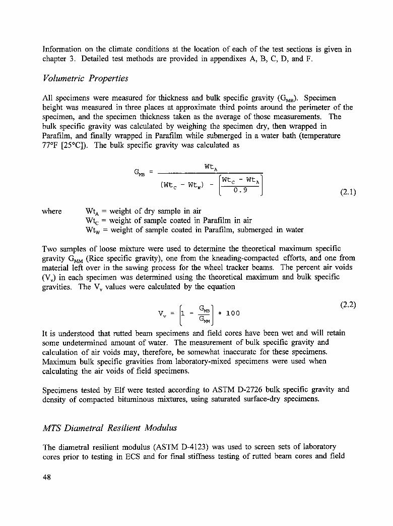
Volumetric Properties
All specimens were measured for thickness and bulk specific gravity (GMB). Specimenheight was measured in three places at approximate third points around the perimeter of thespecimen, and the specimen thickness taken as the average of those measurements. Thebulk specific gravity was calculated by weighing the specimen dry, then wrapped inParafilm, and finally wrapped in Parafilm while submerged in a water bath (temperature77°F [25°C]). The bulk specific gravity was calculated as
Wt AG_ =
- Wt A
(Wtc - wt_) - to. _ (2.1)
where Wta = weight of dry sample in airWtc = weight of sample coated in Parafilm in airWtw = weight of sample coated in Parafilm, submerged in water
Two samples of loose mixture were used to determine the theoretical maximum specificgravity G_n_ (Rice specific gravity), one from the kneading-compacted efforts, and one frommaterial left over in the sawing process for the wheel tracker beams. The percent air voids(Vv) in each specimen was determined using the theoretical maximum and bulk specificgravities. The Vv values were calculated by the equation
(2.2)- * i00
Itis understood thatruttedbeam specimens and fieldcores have been wet and will retain
some undetermined amount of water. The measurement of bulk specificgravityand
calculationof airvoids may, therefore,be somewhat inaccuratefor these specimens.
Maximum bulk specificgravitiesfrom laboratory-mixed specimens were used when
calculating the air voids of field specimens.
Specimens tested by Elf were tested according to ASTM D-2726 bulk specific gravity anddensity of compacted bituminous mixtures, using saturated surface-dry specimens.
MTS Diametral Resilient Modulus
The diametral resilient modulus (ASTM D-4123) was used to screen sets of laboratorycores prior to testing in ECS and for final stiffness testing of rutted beam cores and field
48

sections. Diametral modulus testing is performed on a closed-loop hydraulic system run bycomputer software, which performs the test and calculates the modulus value for eachspecimen.
Each specimen was placed in an environmental cabinet at 77°F (25°C) for at least fourhours prior to testing. The diametral modulus test was performed in accordance withASTM D 4123. A static load of 10 lb. (44.5 N) was applied to restrain the specimen in thetest apparatus. A pulse load was then applied for 0.1 sec. with a 0.9-sec. resting phase.The pulse load was increased until a constant strain condition of 100 _t-strain wasmaintained. The computer software then recorded three consecutive pulse loads of data andcalculated the diametral modulus as the average of those values. The specimen was thenunloaded, rotated 90° within the diametral yoke, and retested. If the two calculated valuesof diametral modulus were within 10 percent of the average of the two values, the averagewas reported as the diametral modulus of the specimen. If the calculated values differed bymore than 10 percent from their average, the specimen was retested.
The diametral resilient modulus was calculated using the following equation:
PDiametral MR = 0.6183
(d _ t) (2.3)
where MR = resilient modulus (psi)P = load (pounds)d = deformation (inches)t = thickness (inches)
The automated data acquisition system used for this testing was developed by Scholz andAb-Wahab (1992). In addition to monitoring the linear variable differential transducers(LVDTs) and load cell outputs, the computer program also displayed the output graphicallyand calculated an approximate modulus value in real time. The data from the last threepulses were saved to hard disk for subsequent calculation of modulus and hard-copy output.
MTS Triaxial Resilient Modulus
Each specimen nominally 4 in. (101.6 mm) in height was also tested to determine resilientmodulus in the triaxial configuration with the MTS apparatus. This test was performedwith a 30-lb. (133.5 N) static load. The pulse loading was increased until either 100 _t-strain or 40 psi (275 kPa) of loading was reached. A value of triaxial resilient moduluswas then calculated by the computer software. The specimen was then further loaded untilthe second condition was reached, and the modulus again calculated. The constant stressand constant strain readings were taken for use in comparison to the ECS resilient modulus,which was taken as constant stress, and the resilient modulus generated by the aging group,which was taken at constant strain.
49

ECS Test
The test procedure for ECS involves inducing and monitoring the water damage to a 4-in.-high × 4-in.-diamter (101.6 mm× 101.6 mm) asphalt-concrete specimen. The specimenwas prepared either by the l_aeading compactor method or by coring from a roller-compacted slab. The procedure for ECS is briefly described in table 2.14. Specimenstested with the ECS are identified in table 2.15.
Figure 2.17 shows a schematic of the equipment used to perform the ECS test program.The system consists of three components: (1) the environmental chamber with controlledtemperature; (2) a fluid-conditioning system, which is essentially a constant headpermeameter with the fluid being either air or water; and (3) a computer-controlled loadingand data acquisition system to monitor the triaxial resilient modulus of the test specimen.
The ECS test quantitatively assesses the effect of water on the stiffness and permeability ofan asphalt-aggregate mixture. Prior to testing with ECS, specimens undergo testing forvolumetric properties and MTS diametral and triaxial resilient modulus as describedpreviously in this chapter. The dry (unconditioned) specimen is then encased in a latexrubber membrane and placed within the ECS. The dry (unconditioned) ECS modulus andair permeability are determined. The modulus test performed by ECS was a triaxialresilient modulus test with a zero confining pressure (i.e., 13"2 = 0"3 = 0). The loading, in theform of a true haversine waveform having a duration of 0.1 sec. followed by a dwell timeof 0.9 sec., was targeted to be 40 psi (275 kPa). Sufficient loading was applied to thespecimen to ensure a constant stress condition before a resilient modulus value wascalculated.
The specimen was vacuum conditioned by applying a vacuum of 20 in. (508 mm) Hg to theoutlet from the specimen in order to evacuate as much air as possible from the specimen.The specimen was then "wetted" by pulling distilled water through it under the action ofthe 20-in. (508 mm) Hg vacuum for 30 minutes. Upon completion of the wetting process,the water permeability of the specimen was determined. The specimen was then subjectedto one of two programs of thermal conditioning cycles.
For specimens that came from environments designated as no-freeze, the specimen wassubjected to three "hot" cycles by heating the specimen to 140°F (60°C) for six hours.During this time, the specimen was subjected to repeated loading of approximately 200 lb.(890 N). Between cycles, the specimen was brought to 77°F (25°C) for at least four hoursand tested for resilient modulus and water permeability. All resilient modulus testing tookplace with the specimen at 77°F (25°C).
For specimens that came from environmental zones with a freeze designation, an additional"freeze" cycle was added at the end of the third hot cycle. The cycle cooled the specimento 0°F (-18°C) for six hours without repeated loading. After the specimen was brought to77°F (25°C) for at least four hours, the resilient modulus and water permeability were againmeasured.
5O

2.14. Summary of the ECS test procedure
Step Description
1 Prepare test specimens per SHRP protocol.
2 Determine the geometric and volumetric properties of the specimen.
3 Encapsulate specimen in silicon sealant and latex rubber membrane, allow to cureovernight (24 hours).
4 Place specimen in the ECS load frame; determine air permeability.
5 Determine unconditioned (dry) triaxial resilient modulus.
6 Vacuum condition specimen (subject to vacuum of 20 in. [508 mm] Hg for 10minutes).
7 Wet specimen by pulling distilled water through specimen for 30 minutes using a20-in. (508 mm) Hg vacuum.
8 Determine unconditioned water permeability.
9 Heat specimen to 140°F (60°C) for six hours under repeated loading. This is ahot cycle.
10 Cool specimen to 77°F (25°C) for at least four hours. Measure triaxial resilientmodulus and water permeability.
11 Repeat steps 9 and 10 for two more hot cycles.
12 Cool specimen to 0°F (-18°C) for six hours without repeated loading. This is afreeze cycle.
13 Heat specimen to 77°F (25°C) for at least four hours and measure the triaxialresilient modulus and water permeability.
14 Split specimen and perform a visual evaluation of stripping and binder migration.
15 Plot the ECS resilient modulus ratio.
Scholz et al. 1992.
51

Table 2.15. Experiment design for the ECS testing for SHRP A-003A Task C.5I
Mixture Number Mixture Code Site Replicate
1 AB5R803 AB52 AB5R804
3 AB5KL01
4 AB5KM035 AB5KH066 AB5KD08
7 AZ5R804 AZ5 AZ5RS038 AZ5R8059 AZ5KL01
10 AZ5KM0411 AZ5KH0512 AZ5KH06
AZ5KD07
13 CABKL02 CAB14 CABKM1215 CABKM 1416 CABKD05 CABKH04
17 CADR804 CAD18 CADRS0619 CADKL02
20 CADKM0421 CADKD0722 CADKD08 CADKH05
23 CAGR803 CAG24 CAGR80525 CAGKL01
26 CAGKM04
27 CAGKD0628 CAGKD07
29 GAAR803 GAA30 GAAR80631 GAAKL12
32 GAAKM1133 GAAKH0434 GAAKD01
52
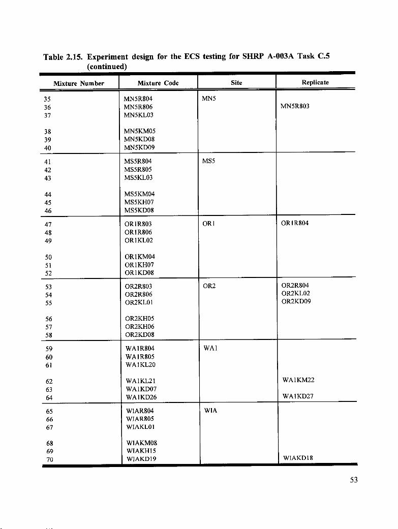
Table 2.15. Experiment design for the ECS testing for SHRP A-003A Task C.5(continued)
Mixture Number Mixture Code Site Replicate
35 MN5R804 MN536 MN5R806 MN5R80337 MN5KL03
38 MN5KM0539 MN5KD0840 MN5KD09
41 MS5R804 MS542 MS5R80543 MS5KL03
44 MS5KM0445 MS5KH0746 MS5KD08
47 OR1R803 OR1 OR1 R80448 OR1R80649 OR1KL02
50 OR 1KM0451 OR1KH0752 OR1KD08
53 OR2R803 OR2 OR2R80454 OR2R806 OR2KL0255 OR2KL01 OR2KD09
56 OR2KH0557 OR2KH0658 OR2KD08
59 WA 1R804 WA 160 WA1R80561 WA1KL20
62 WA 1KL21 WA 1KM2263 WA 1KD0764 WA1KD26 WA1KD27
65 WIAR804 WIA66 WIARS0567 WIAKL01
68 WIAKM0869 WIAKH 15
70 WIAKD 19 WIAKD 18
53

54

At the completion of either three or four conditioning cycles, the specimen membrane wasremoved, and the specimen was split diametrally using MTS. A visual evaluation ofstripping and binder migration was made from the two split faces of the specimen.
OSU Wheel Tracking Test
The procedure for the OSU wheel tracking test involved conditioning beams of asphalt-aggregate mixtures to induce water damage and then testing them under repeated loading ofthe OSU wheel tracker. Rut depth was the response mode monitored. Figure 2.18 shows aschematic of the OSU wheel tracker. The procedure is briefly outlined in table 2.16. Thebeam specimens tested under this conditioning procedure and their associated rutted beamspecimens are identified in table 2.17.
After volumetric data was obtained for the beam specimen, it was subjected to a waterconditioning program analogous to that within ECS. There were, however, the followingminor differences:
1. The wetting procedure for the beam specimens employed a slightly higher vacuumlevel and was significantly longer than that employed in ECS. This was to ensurethat specimens achieved a saturation of between 60 percent and 80 percent.
2. The duration of some of the conditioning cycles was longer than in the ECSprocedure because of scheduling constraints for the equipment used for thermalconditioning.
3. The order of the conditioning cycles was slightly different for the wheel tracking testprogram relative to the ECS test program. Again, this was due to schedulingconstraints on the equipment used for thermal conditioning.
Once the beam had undergone water and thermal conditioning, it was wrapped in plastic, toprevent moisture loss and placed in the mold of the OSU wheel tracker. Thin, expandedfoam sheets were placed between the beam and the mold wall to prevent movement of thebeam under the action of the rolling wheel. An 1/8-in.-thick (3 mm) piece of teflonsheeting was placed between the specimen and the OSU wheel tracker platen to provide africtionless interface. The mold and beam were placed in the OSU wheel tracker, boltedinto place, and the system was brought up to the test temperature of 104°F (40°C) for atleast two hours.
After the specimen reached testing temperature, as determined by a thermocouple probeinserted into a hole drilled in the beam, the plastic wrap was removed from the top of thebeam to prevent the plastic from being picked up by the pneumatic tire. Testing thenbegan.
55

Tire TireRail
Stub axleStub axle
Swivel
Swivel
Jack Jack
Telescopic arm
Schematic
Control /Panel Pneumatic
_ _. _. . . Tire
Specimen"" Holder,
i
Side View
Figure 2.18 Schematic of the OSU wheel tracker
56

Table 2.16 Summary of OSU wheel tracking test procedure
Step Description
1 Prepare test specimen as described in Table 2.11.
2 Determine the gravimetric properties of the beam.
3 Place a latex and silicone sealant seal around the circumference of the beam at midheight andallow to cure overnight (24 hours).
4 Wet the beam specimen by pulling distilled water through the specimen under a 23-in. (584 mm)
Hg vacuum until a degree of saturation of at least 60% is obtained, but for not more than 2hours.
5 Subject the wet beam specimen to wet thermal conditioning cycles as followst:Heat the specimen to 140°F (60°C) in a distilled water bath for 6 hours.Cool the specimen to 77°F (25°C) in a distilled water bath for 10 hours.Heat the specimen to 140°F (60°C) in a distilled water bath for 6 hours.Cool the specimen to -4°F (-20°C) in a distilled water bath for 8 hours.Heat the specimen to 140°F (60°C) in a distilled water bath for 10 hours.
Cool the specimen to 77°F (25°C) in a distilled water bath for 10 hours.
6 Wrap the specimen in plastic (e.g., Saran Wrap) to retain moisture during the testing phase.
7 Place the conditioned beam specimen in the rutting tester and heat the specimen to 104°F (40°C).
8 Perform the OSU wheel tracking (rutting) test on the conditioned beam specimen until 10,000wheel passes have elapsed taking rut depth measurements at 0, 200, 500, 1,000, 2,000, 5,000, and10,000 wheel passes.
9 Plot the rut depth versus wheel passes.
10 Core the rutted beam specimen along the wheel track so as to obtain cores for evaluation. Splitthe cores and perform a visual evaluation of stripping and binder migration.
Source: Scholz et al. 1992.
1For mixtures from no-freeze environments, eliminate the -20°C (-4°F) cooling cycle.
57

Table 2.17 Experiment design for the OSU wheel tracking for the SHRP A-003ATask C.5
Mixture Number Mixture Code Site Replicate
1 AB5R8011 AB5 AB5R802
2 AZ5R801 AZ5 AZ5R802
3 CADR801 CAD CADR802
4 CAGR801 CAG CAGR802
5 GAAR801 GAA GAAR802
6 MN5R801 MN5 MN5R802
7 MS5R801 MS5 MS5R802
8 OR1R801 OR1 OR1R802
9 OR2R801 OR2 OR2R802
I 0 WA 1R801 WA1 WA 1R802
11 WIAR801 WIA WIAR802
_Each beam resulted in three cored, rutted beam specimens (e.g., AB5R801A, AB5R801B, AB5R801C).
A preconditioning wheel load of 50 wheel passes at 92 psi (634 kPa) was applied to the
beam specimen to eliminate the high plastic deformations characteristic of asphalt-aggregate
mixtures at the onset of loading. After the preconditioning load was completed,
measurements were obtained to establish the baseline beam surface profile. These
measurements were obtained electronically (i.e., via computer), using a displacementtransducer designed specifically for these measurements, or manually, using the caliper
provided by LCPC. Figure 2.19 shows the 15 positions at which the surface profile
measurements were obtained. Note that the measurement positions were concentrated near
the center of the beam along its longitudinal axis so as to avoid measurement of high
plastic deformations that occur in the region where the rolling wheel slows down, stops,and reverses direction at the end of the travel path.
The wheel loading was then increased to 100 psi (689 kPa) and reapplied. Testingproceeded with application of up to 10,000 wheel passes or, alternatively, until failure
occurred (as established by a sudden and significant increase in plastic deformation). After
accumulation of 100, 200, 500, 1,000, 2,000, and 5,000 wheel passes the load was
temporarily halted and the surface profile measured. After 10,000 wheel passes or when
loading was terminated because of failure, a final surface profile was measured. The beam
was then cored into three, 4-in.-diameter (101.6 mm) rutted beam specimens.
58

Elf Wheel Tracking Test
The procedure for the Elf wheel tracking test involved testing a specimen immersed in awater bath at elevated temperatures. A brief summary of the test procedure is given intable 2.18. Appendix F provides the detailed test protocol. Mixtures tested in thisprocedure are listed in table 2.19.
The Elf wheel tracker employed an 8-in.-diameter (203.6 mm), 1.85-in.-wide (47.0 mm)steel wheel. The wheel was applied to the surface of the specimen with a 156-1b. (697 N)force. The wheel reciprocated over the specimen, making 50 passes per minute, at amaximum speed of 1.1 ft./sec. (340 mm/sec.), reached at the midpoint of the specimen.The configuration resulted in a 0.1-sec. loading period and a 1.0-sec. relaxation period atthe midpoint of the specimen. An LVDT was mounted to measure the movement of thewheel downward as the rut depth increased.
The test specimens were 10.24 in. + 0.1 in. (260 mm + 2 mm) wide, and 12.6 in. + 0.1 in.(320 mm + 2 mm) long. The thickness of the specimen was typically twice the maximumnominal aggregate size, ranging from 1.5 in. to 3.9 in. (38 mm to 100 mm). The specimenwas mounted so that it is surrounded on all sides by a minimum of 0.79 in. (2 cm) of free-circulating water.
Elf identifies the following additional data, as well as rut depth:
• Postcompaction consolidation. The depth of impression that rapidly accumulatesduring the first 1,000 _+500 wheel passes.
• Creep slope. The inverse rate of deformation expressed in units of wheel passes permillimeter of deformation. This rate is calculated after the postcompactionconsolidation but before the onset of moisture damage.
• Stripping inflection point. The number of wheel passes necessary to induce moisturedamage to the specimen. After moisture damage begins, the rate of deformationincreases rapidly, and uncoated aggregate particles emerge from the surface of thespecimen.
• Stripping slope. The inverse rate of deformation measured after the strippinginflection point until the end of the test.
59

5.9 in. 3.5 in. 3.5 in. 5.9 in.
(150 ram) (90 ram) (90 ram) (150 ram)
•._._._._..._._:_:_._._:_:_._._._._._._L_:._./.[._._._-..._._...._:_.[_:_._._._._.._.._._..:._]_
i;ii;:ii;:;;;iiii__i_iiiii_i_:i_illiiillii_iiiiiiliiiilliiii_ii_iiiiiii!_ii!i_i?::i_}i}iil)i;iii}i;i;}i}i}i;i;i}i}iiiiiiiiili?iiliii
::::::: ::: ::: ::::::::::::::::::::::::::::::::::::::::::::::::::::::::::::::::::::::::::::::::::::::_:::::::::::
:::_iiii_i:::_;!_i_i_:i_;_:;:i_:_i_iiiiii:i:::i:iii:::i_i:_i:_i:i_:iiii_iii_:_!:i:i_iii_:_iiiii_2_iiii_iii_
Rut 1V[easurement Region o_ HighO _tline Position Plastic Deformation
(Both Ends)
a)PlanView
Wheel Travel / i
17.7 in. (450 ram) _ /
...._ i /ii_i_i_i_i_iii_iiiii_iii_i!i_i_iiiiii!!_!__i_!ii!iiiiiiii_iiiii_i_ii!___i!!!!_i!ii!!_!i!i_i!__i_!_ii!!i_!!______i!i!iii_i!i!i!_!_!ii!iii_i!i!i!iiii_ii!_!!_____!!ii_i!!!!i!I_i_i_i_i_iii_i_]_i_i_iiiii_i_i_i_i_i_i_i_i_i_iiiii_i_iii_i_ii_i_._iiiiiii_iiiii_i!iii_i_iii_i_ii_i_ii!_iiiiiii_iii_iiiii_iiiiiii_iiiiiii!iiii_
,!i_iii_i_iii_i_i_i_i_i_i_i_i_i_i_iiiiiiiii_i!i_i_i_i_i_i_iiiii_i_i_iiiiiiiiiiiiiiiiiiiii!iiiiiiiiiiiiiiiiiiiiiiiiiiiiiiii!iiiiiiiiiiiiiiiiiiiiiiiii_i_iiiiiii_i_iii_i_!_i_i_b) El_-vation View
Figure 2.19 Measuring positions for rut depth
6O

Table 2.18 Summary of the Elf wheel tracking procedure
Step Description
1 Prepare test specimen according to standard Elf Protocol (appendix E).
2 Determine the gravimetric properties of the specimen.
3 Mount the specimen into the test mounting tray using plaster of paris.
4 Bolt the specimen tray into the wheel tracker, introduce water into the machine.
5 Determine test temperature:
104°F (40°C) for binders of viscosity grade AC-l 0 (penetration grade 120/150) or softer122°F (50°C) for all harder grade of binder
6 Stabilize water bath temperature at test temperature. Condition specimen by soaking at testtemperature for 30 _+5 minutes.
7 Lower wheel onto specimen and begin testing. Ten wheel passes is used as the test zero.
8 Record rut depth after at least every 100 wheel passes. Note number of passes at which strippedaggregate particles are ejected from the specimen into the water bath.
9 Conclude testing after 20,000 passes, or when a 20 mm rut depth is reached.
Table 2.19 Experiment design for the Elf wheel tracker
Mixture Number Mixture Code Site
1 AB5ELF01 AB5
2 AZ5ELF01 AZ5AZ5ELF02
3 OR1ELF01 ORIOR 1ELF02
4 OR2ELF01 OR2OR2ELF02
5 WIAELF01 WIAWIAELF02
61

Visual Evaluation of Stripping and Binder Migration
After each testing procedure was completed, and the specimen had been tested for resilientmodulus with either MTS or ECS, a visual evaluation was performed. Specimens weresplit in half by applying a diametral static load. The two broken faces were examined todetermine what percentage of the surface area of the face had been stripped of asphalt. Thepercentage of stripping was reported to be: 0, 5, 10, 20, 30, 40, or 50, as shown in figure2.20. Fractured faces were neglected in the identification of aggregate faces that had losttheir asphalt covering.
In addition to percent of stripped aggregate, it became evident early in the testing programthat some of the field validation mixtures had experienced displacement of the asphaltbinder in the direction of water flow through the specimen during the ECS test procedure.This phenomenon, termed binder migration, is described by giving the specimen a letterrating, each letter corresponding to a level of binder movement, as represented in figure2.21.
62

5% 10%
20% 30%
40% 50%
Figure 2.20. Visual stripping rating chart
63

A B(1-10% migration) (10-20% migration)
l Flat black,"flowed"asphalt4"
Shinyblack,
may be stripped
4" "="-i=,,,"-
C D(20-30% migration) (30-40% migration)
E F(40-50% migration) (>50% migration)
!ii!i!i!!i_:::::::::::;i:i:[:i:i:?:.
!iiiilg!iiiiii:.:.:,:.:.:.:.:.:..
.:.:,:.:.:.:.:.:.:.:.:.:..,::::::::::::::::::::::::::::::: :':':':':':':':':
Figure 2.21. Binder migration rating chart
64

3
Results
This chapter presents the results of the field validation effort for water sensitivity. Includedare results obtained in the Environmental Conditioning System (ECS) and the Oregon StateUniversity (OSU) wheel tracking programs conducted at OSU, as well as those obtained bythe Elf Asphalt wheel tracking program. Resilient modulus data, both diametral andtriaxial, from cores taken from in-service field test sections are also presented.
ECS Test Program
The specimens tested in the ECS program are summarized in table 3.1. The initial testprogram included six specimens from each mixture, with the exception of CAB, for whichthere were four specimens. Additional specimens were added to investigate mixtures thathad data that varied within the mixture set. The test results for the ECS testing programare shown graphically in figures 3.1 through 3.12.
ECS Modulus Data
Each data curve in figures 3.1 through 3.12 represents a single ECS specimen. The curvesdefine the change in retained resilient modulus (termed ECS-modulus ratio) as a function ofthe conditioning level (each cycle represents a conditioning cycle within ECS with the firstthree cycles being "hot" cycles and the fourth cycle being the "freeze" cycle) _. Theretained resilient modulus, or ECS modulus, ratio is defined as the ratio of the conditionedresilient modulus to the unconditioned modulus and is measured at the end of each
conditioning cycle. The ECS modulus ratio provides an indication of the amount ofstiffness loss in the specimens caused by water damage relative to the dry, unconditionedstiffness of the specimen. Water damage as measured by the decrease in the ECS modulus
1 The resilient modulus obtained in the ECS is termed the ECS modulus to distinguish itfrom the traditional diametral and triaxial resilient moduli, as well as the dynamic modulus.The ECS modulus is a triaxial resilient modulus with zero confining stress (i.e., cr2 = _3 -- 0)conducted on a 4-in.-diameter (102 mm) x 4-in.-high (102 mm) asphalt-aggregate mixture testspecimen.
65

Table 3.1. ECS test specimens
Visual
Air Degree of
Specimen Voids Stripping Binder(%) (%) Migration _ Comments
AB5R803 5.5 5 No
AB5R804 5.3 5 NoAB5KL01 6.0 5 C
AB5KM03 4.4 5 DAB5KH06 2.8 5 EAB5KD08 2.6 5 E
AZ5R803 8.3 20 NoAZ5R805 8.2 20 NoAZ5KL01 8.4 20 No
AZ5KM04 8.0 20 No
AZ5KH05 6.2 20 CAZ5KH06 6.3 20 C
CABKL02 7.4 5 CCABKM12 4.9 5 DCABKM14 6.0 5 E
CABKH04 4.1 5 DCABKD05 4.0 5 C
CADR804 9.4 5 NoCADR806 9.7 5 NoCADKL02 9.5 5 No
CADKM04 9.1 5 NoCADKH05 7.8 5 NoCADKD07 8.5 5 NoCADKD08 7.7 5 No
CAGR803 11.0 20 NoCAGR805 10.7 20 No
CAGKL01 9.3 30 No
CAGKM04 8.8 20 NoCAGKD06 7.8 30 A
CAGKD07 7.0 20 BI
66

Table 3.1. ECS test specimens (continued)
Visual
Air Degree of
Specimen Voids Stripping Binder(%) (%) Migration I Comments
GAAR803 7.6 0 NoGAAR806 9.1 0 NoGAAKL12 9.8 5 No
GAAKM 11 9.2 0 NoGAAKH04 7.4 0 No
GAAKD01 6.4 5 No
MN5RS03 11.3 5 NoMN5R804 10.6 5 NoMN5R806 11.7 5 No
MN5KL03 6.5 5 DMN5KM05 5.6 5 D
MN5KD08 4.4 5 DD
MN5KD09 3.0 5
MS5R804 7.6 20 NoMS5R805 8.0 20 NoMS5KL03 6.9 20 A
MS5KM04 5.9 20 C Failed 1st cycle-loading continued 2MS5KH07 4.1 20 C Failed 1st cycle-sample removed 2MS5KD08 3.5 20 C Failed 1st cycle-loading continued 2
OR1R803 8.3 5 NoOR1R804 7.4 0 NoOR1R806 7.3 5 No
OR 1KL02 11.6 5 NoOR1KM04 9.2 0 BOR1KH07 7.0 0 C
ORIKD08 6.8 0 C
OR2R803 21.3 10 NoOR2R804 20.2 5 NoOR2KL02 19.6 20 No
OR2KH05 17.3 5 NoOR2KH06 16.2 5 NoOR2KD08 18.1 10 NoOR2KD09 16.7 5 No
67

Table 3.1. ECS test specimens (continued)
Visual
Air Degree ofSpecimen Voids Stripping Binder
(%) (%) Migration I Comments
WA IR804 7.0 0 NoWA1R805 6.6 0 NoWA 1KL20 11.4 5 D
WA1KL21 10.3 5 EWA1KM22 10.3 5 EWA 1KD07 7.3 5 E
WA 1KD26 8.6 5 FWA 1KD27 9.1 5 F
WIARS04 3.4 5 NoWIAR805 3.5 5 No
WIAKL01 3.3 5 No Failed 1st cycle-loading discontinued 2
WIAKM08 1.8 5 No
WIAKH15 1.4 5 No Failed 2nd cycle-loading continued 2WIAKD 18 0.6 5 NoWIAKD19 0.7 5 No
1Figure 2.21 illustrates the rating scale for binder migration./Failed because of excessive deformation under repeated axial loading.
68

1.2
1.0
o 0.8
N 0.60
o 0.4W
0.2 AirVoidsR5.6% R5.3% 6.0% 4.4% 2.8% 2.6%
0.0 _ i I I0 1 2 3 4 5
Cycle
Figure 3.1. AB5 ECS results1.2
o1"0_
_0.8¢=::u_ __m
0.6qD0
U)o 0.4I,IJ
0.2 Air VoidsR8.3% R8.2% 8.4% 8.0% 6.2% 6.3%
0.0 i0 1 2 3 4
CycleFigure 3.2. AZ5 ECS results 69

1.2
1.0 =
o_ O.8
= 0.60
o 0.4
0.2 Air Voids7.4% 6.0% 4.8% 4.1% 4.1%
0.0 I I i i0 1 2 3 4 5
CycleFigure 3.3. CAB ECS results
1.2
1.0
o. .8
0.6
¢_ 0.4IJJ
0.2 Air VoidsR9.8% R9.5% R9.4% 9.1% 8.5% 7.8% 7.7%
0,0 r J0 1 2 3 4 5
CycleFigure 3.4. CAD ECS results70

1.2[
1.0 •
oN.'_ 0.etic
= 0.60
O 0.4 _ .,_IJ.l
0.2 Air VoidsRll.0% R10.7% 9.3% 8.8% 7.8% 7.0%
i -e- o -B--_---_0.0 _ i I
0 1 2 3 4
Cycle
Figure 3.5. CAG ECS results
1.2 _ _[]1.0
_._o 0.8 _---_ -_¢ni
= 0.6"005(/)
0.4UJ
0.2 Air VoidsR9.1% R7.6% 9.8% 9.2% 7.5% 6.4%
-B- --e-- o -I_--_-X--0.0 i l
0 1 2 3 4
CycleFigure 3.6. GAA ECS results 71

1.2
0 1"0
0.6
,,, 0.4
0.2 Air VoidsRll.3% R10.6% Rll.7% 6.5% 5.6% 4.4% 3.0%
0.0 I I i ,0 1 2 3 4 5
CycleFigure 3.7. MN5 ECS results
1.2
1.0 '
0.6 _ -_ i0 "'E):S(/)o 0.4l.U
0.2 Air VoidsR8.0% R7.6% 6.9%
t-_- o0.0 _ i I
0 1 2 3 4
CycleFigure 3.8. MS5 ECS results72

1,2
1.o ..a 0 o
0
: 0.8
= 0.6"O0
if)o 0.4W
0.2 Air VoidsR8.3% R7.4% R7.3% 11.6% 9.2% 7.0% 6.8%
-!- _ o -t_-e-_--I-0.0 i i i
0 1 2 3 4
CycleFigure 3.9. OR1 ECS results
1.2
10O
0.8
=1
= 0.6"00=S(/)o 0.4IJ.i
0.2 Air VoidsR21.2% R20.2% 19.6% 18.1% 17.3% 16.2%-B- -_- o -B--_---X-
0.0 _ i I [0 1 2 3 4 5
CycleFigure 3.10. OR2 ECS results 73

1.2
1.0 _ ___(_o 0.8
_ 0.6"O0
o 0.4W
0.2 Air VoidsR7.0% R6.6% 11.4% 10.3% 10.3% 9.1% 8.6% 7.3%
0.0 , i I I0 1 2 3 4 5
CycleFigure 3.11. WAI ECS results
1.2
1.0
O
. 0.8
0.6 nO
¢Do 0.4UJ
0.2 Air VoidsR3.6% R3.4% 1.8% 0.7% 0.6%
0.0 i i i i0 I 2 3 4 5
CycleFigure 3.12. WIA ECS results74

ratio may be the result of a loss of adhesion between the asphalt and the aggregate, a lossof cohesion in the asphalt binder, or both. During testing in ECS, specimens of twomixtures experienced excessive deformation during the "hot" cycles of the test: WIA andMS5. This behavior had not occurred during the previous work with the Strategic HighwayResearch Program (SHRP) core asphalts and aggregates. For the purposes of this report,specimens that deformed excessively within the ECS (defined as a loss in sample height ofbetween 5 percent to 15 percent, so that the yoke that holds the linear variable differentialtransducers (LVDTs) to the specimen could no longer be mounted) were considered"failed" and were not used for the statistical analysis that follows.
In some cases, failed specimens were left in the ECS for further conditioning, without therepeated loading, even though it was impossible to take further modulus readings. In othercases, the repeated loading was stopped before the specimen had deformed to the extentthat modulus testing was impossible, and the specimen was further conditioned withoutloading, with modulus testing taking place between cycles. The data for these specimensalso appear in appendix C. The specimens that experienced failure because of excessivedeformation within the ECS test apparatus are identified in table 3.1.
Visual Degree of Stripping and Binder Migration Data
The visual degree of stripping, as evaluated after the completion of the ECS procedure,indicates the level of adhesion loss between the asphalt binder and the aggregate in aspecimen. Binder migration may be the result of both a loss of adhesion between theasphalt binder and the aggregate and a loss of cohesion in the asphalt binder. In order forasphalt binder particles to migrate within the specimen, the particles must first debond fromall surrounding material. This debonding includes both loss of adhesion between the binderand the aggregate and loss of cohesion between binder particles. The complete data setfrom the ECS testing program is included in appendix C.
Permeability Data
Average values of the coefficients of permeability and the intrinsic permeabilities for allmixtures are reported in table 3.2. The coefficients of air and water permeability werecalculated using Darcy's Law. The coefficient of permeability is dependent on both themedia and the fluid used as a permeant. The intrinsic permeability is a property of themedia only. The two terms are related as follows:
k = K Y (3.1)i.t
where k = coefficient of permeability (m/s)K = permeability (m2)7 = specific weight of the fluid (N/m 3)
= viscosity of the fluid (N-s/m 2)
75

Table 3.2. Average coefficients of permeability, intrinsic permeabilities for eachmixture 1
Mixture Coefficient of Intrinsic Coefficient of Intrinsic
Permeability, Permeability, Permeability, Permeability,Air Air Flow Water Water Flow
(cm/sec.) (cm 2) (cm/sec.) (cm 2)
AB5 3.89E-06(1) 2 6.15E-10 (1) 1.84E-05 (3) 1.68E-10 (3)
AZ5 2.29E-05 (4) 3.63E-09 (4) 7.82E-05 (4) 7.13E-10 (4)
CAB 7.08E-06 (1) 1.12E-09 (1) 1.41E-05 (1) 1.28E-10 (1)
CAD 6.97E-05 (7) 1.10E-08 (7) 1.60E-04 (7) 1.46E-09 (7)
CAG 4.59E-05 (6) 7.26E-09 (6) 2.18E-04 (6) 1.98E-09 (6)
GAA 5.50E-05 (6) 8.69E-09 (6) 3.40E-04 (6) 3.10E-09 (6)
MN5 5.98E-05 (4) 9.47E-09 (4) 3.55E-04 (4) 3.23E-09 (4)
MS5 9.57E-06 (1) 1.51E-09 (1) 6.30E-05 (2) 5.74E-10 (2)
OR1 4.04E-05 (4) 6.39E-09 (4) 5.82E-04 (5) 5.30E-09 (5)
OR2 8.10E-05 (4) 1.28E-08 (4) 1.78E-03 (5) 1.63E-08 (5)
WA1 1.00-05 (3) 1.59E-09 (3) 9.66E-05 (3) 8.80E-10 (3)
WIA __3 ......
1For new, unconditioned, laboratory-fabricated specimens.2Indicates number of specimens represented in average.3Indicates permeability too low to read with ECS apparatus.
76

It was not uncommon for specimens to have coefficient of permeability values too low forthe ECS equipment to measure, for both air and water. Of the 78 specimens tested, 37were impermeable to air in the ECS apparatus and 32 were impermeable to water. Thelower limits of the ECS permeability apparatus are approximately 1.14E-07in./sec. (7.90E-07 cm/sec.) for air and 7.87E-08in./sec. (2.00E-07 cm/sec.) for water. Also, five of thespecimens tested were impermeable to air, and yet permeable to water after the 30-minutewetting procedure.
Figure 3.13 shows the relationship between the coefficient of permeability for air and thepercent air voids. Similar data for the coefficient of permeability for water are shown infigure 3.14. These data are for new, laboratory-fabricated specimens. For both air andwater flow, the coefficient of permeability tends to increase with increasing air voids.
Figures 3.15 through 3.26 show the variation of the coefficient of permeability of waterthroughout the ECS test procedure.
OSU Wheel Tracking Program
Results from the OSU wheel tracking program are summarized in table 3.3 and are showngraphically in figure 3.27. Table 3.4 shows the data from the cores taken from the ruttedbeam specimens. It should be noted that the beam designated CADR802 was loadedincorrectly during testing and therefore has been dropped from the analysis of the data.Each beam represents a unique specimen, and its rut depth will be used for statisticalanalysis. The average rut depth of two specimens from the same mixture is only used infigure 3.27 for illustration.
Two mixtures produced specimens that failed within the OSU wheel tracker, CAG, andMN5. Failure is defined as a rut depth of greater than 20 mm (0.79 in.). The beams madeof the MN5 mixture failed within 1,000 wheel passes, and testing was discontinued. Thebeams manufactured using the CAG mixture failed within 2,000 wheel passes, and testingwas discontinued at 5,000 wheel passes.
A visual degree of stripping was not obtainable for the OR2 beam specimens because thepowder used on the surface of the beam to prevent adhesion between the beam and thepneumatic tire of the OSU wheel tracker migrated down into the specimen. It wasimpossible to judge the stripping under these conditions.
Elf Wheel Tracking Program
The results of the testing conducted by Elf Asphalt in Terre Haute, Indiana, are presented intable 3.5 (Hines 1992). Rut depths at wheel pass levels corresponding to those used in theOSU wheel tracking test have been plotted for each specimen tested by Elf in figure 3.28.
77

Field Data
Weather Data
Data from the nearest recording weather station for each field section are presented intables 3.6 through 3.9. The most recent full year of data published by the NationalClimatic Data Center is 1990. Eleven of the 12 sites were in place during the full 1990
calendar year.
Project CAG was constructed in late summer of 1990. The 30-year data are presented toindicate more stabilized information from the site in case the 1990 data represent abnormal
temperature or precipitation extremes.
Traffic Data
Traffic data for each field test section as reported by the local state agency are shown intable 3.10. Average daily traffic (ADT) and percentage of truck traffic were requested forthe most recent full year of data available. In some cases, the data are for a year prior tothe construction of the test section investigated in this program.
Manual Distress Surveys and Pasco Data
Table 3.11 indicates the condition of each field test section from the most recent distress
survey, manual or Pasco, for the site. The type of survey and date performed are alsoindicated.
Field Core Data
The results of the MTS diametral and triaxial resilient modulus testing of the cores takenfrom field sites are shown in figures 3.29 through 3.50. The MTS modulus values of newlymanufactured, laboratory kneading compactor cores are shown as a reference. Thismodulus is termed the unconditioned modulus value because the specimens have not
undergone any type of conditioning prior to this measurement of modulus. The results ofthe visual stripping evaluation are shown in table 3.12. The complete data from the coresare given in appendix D.
78
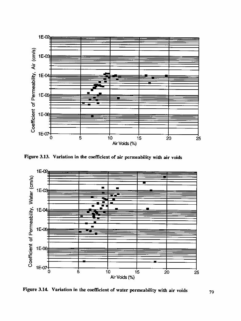
1E-02
E 1E-0_Ov
I,_°_
<
1E-0_ "_._
ID N1F_E •I.- •
m 1E-05 --_---
0 •
C
m IE-0£_____.__.O
O
1E-070 5 10 15 20 25
Air Voids(%)
Figure 3.13. Variation in the coefficient of air permeability with air voids
1E-0_
E "¢J
v l I
,_ 1E-0_==_:::m::: _tm_======
- _m • m
• m •
1E-04 "--J=" " --.m
n
E -_ 1E-05
O
e-.__ 1E-06
(DO -- •
O 1E-O_0 5 10 15 20 25
AirVoids (%)
Figure 3.14. Variation in the coefficient of water permeability with air voids 79

1.0E-0_- Air Voids
E R5.6%o 1--- .u_--uc>" R5.3%
,m
1 6.0%
n "_ 4.4%o 1"E 2.6%
0
10 1 2 3 4
ECS Cycle
Figure 3.15. Variation in the coefficient of water permeability in the ECS procedure, AB5
1.0E-0& Air Voids
_" R8.3%E 1.0E-O_:
8.2 %
8.4 %
- 8.0o/°Q_
-.-, t 6.3%¢" l
sO s
_ t0 sI0 t
II
I
0 2 3 4ECS C_cle
Figure 3.16. Variation in the coefficient of water permeability in the ECS procedure, AZ580

1.0E-02Air Voids
7.41%
'1.0E-03._, 6.04%
,m
"_ 1.0E-04 4.14 %
0)13_
o 1 _.,._ ,._ _
.__ •tO • %
8 1 st "•t %
J %• %
J •j _ ,t •
0 1 2 3 4ECSCycle
Figure 3.17. Variation in the coefficient of water permeability in the ECS procedure, CAB
1.0E-02Air Voids
R9.8%.---.1.0E-03 ..,,,_
"1_ 9.5%
=9.4%o9.1%
"6 --N-E _ 8.5%
7.8 %O
1.(0 1 2 3 4
ECSCycle
Figure 3.18. Variation in the coefficient of water permeability in the ECS procedure, CAD81

1.0E-02 Air Voids
R 11.0%
R 10.7%
• """""'_' 9.3 %
°#- I 88%'5 1 L._, e.,,.,.='--_" 7.8 %"O
8 7.0%O1
10 1 2 3 4
ECSCycle
Figure 3.19. Variation in the coefficient of water permeability in the ECS procedure, CAG
1.0E-02 Air Voids
R7.6%L
'1.0E-03,,_, R9.1%
1.0E-04_"'-_ 9.80/0
9.2 %
"5 1.0E-05= 7.5 %
6.4%O 1.0E-0E
1.0E-010 2 3 4
ECSCycle
Figure 3.20. Variation in the coefficient of water permeability in the ECS procedure, GAA82

1.0E-02.. Air Voids
11.7%
1.0E-0_ .-,,,-_ -- Rll.3%
-"_ _ R 10.6%cD
.. 6.5 %0_.. -o
= 4.4 %_D
•o _ _'------..-...._ ..,,-
q,J 3.0 %0
o S1
0 1 2 3 4ECSCycle
Figure 3.21. Variation in the coefficient of water permeability in the ECS procedure, MN5
1.0E-02: Air Voids
R8.0%
I.0E-0_ -4--R7.6%
l. .."_ 1 : 6.9%
# - 5.9 %o_ "I"
e--
°ol /
O#
#
0 1 2 3 4ECS C_cle
Figure 3.22. Variation in the coefficient of water permeability in the ECS procedure, MS583

Air Voids
11.6%
92%1 , R8.3%
n R 7.4%
¢- 7.3 %.mO
o 6.8 %
O 1.0E-061.0E-0_
0 1 2 3 4ECSCycle
Figure 3.23. Variation in the coefficient of water permeability in the ECS procedure, OR1
1L , Air Voids
l__ R21.3%,_, R20.2 %
19.6%
n 18.1%o_- 17.3%.__
16.2%(.3
,/0 1 2 3 4
ECSCycle
Figure 3.24. Variation in the coefficient of water permeability in the ECS procedure, OR284

1.0E-0_ Air Voids
11.4%
'1.0E-0_ -,,,-10.3 %
_ 1.0E-(N _ f"_""""-"--- _ 7.0%d_ Q
m t 6.6 %13- t
o 1.0E-0_ et- I
o Io 1.0E-06 t
II
ll
I1.0E-0;
0 2 3 4ECSCycle
Figure 3.25. Variation in the coefficient of water permeability in the ECS procedure, WA1
1.0E-02=. Air Voids
R3.5%
'1.0E-03 .-,,,-R 3.4%
"_ 1.0E-04a)
13_
"_ 1.0E-05
_ sj"_ sS
° /0
/0 1 2 3 4
ECSCycle
Figure 3.26. Variation in the coefficient of water permeability in the ECS procedure, WIA85

Table 3.3. Summary of OSU wheel tracking specimens
Visual Degree ofAir Voids Percent Saturation Stripping
Specimen (%) (%) (%)
AB5R801 6.6 59 5AB5R802 6.5 64 5
AZ5R801 8.5 73 10AZ5R802 8.2 61 10
CADR801 9.7 68 5CADR802 9.7 71 5
CAGR801 12.0 69 30CAGR802 12.0 69 30
GAAR801 8.1 59 0GAAR802 7.4 62 0
MN5R801 12.1 48 5MN5R802 10.7 52 5
MS5R801 8.4 66 20MS5R802 8.3 45 10
OR1RS01 8.4 61 5OR1R802 8.4 64 5
OR2R801 21.4 22 __l
OR2R802 22.2 23 --
WA 1R801 6.6 40 0WA 1R802 6.0 42 0
WIARS01 4.4 43 5WIARS02 3.8 43 5
1Unable to distinguish stripping because of migration of dust into specimen
86
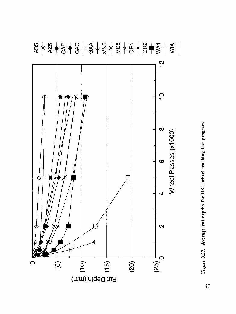
O4
0

Table 3.4. Summary of data from rutted beam cores
MTS Diametral
Air Voids Height ModulusSpecimen (%) (in.) (ksi)
AB5R801A 4.5 3.453 162.0AB5R801B 5.0 3.319 163.0AB5R802A 4.5 3.094 170.0AB5R802B 4.5 3.534 167.0
AZ5RS01A 9.5 3.078 757.5AZ5R801B 8.5 3.316 836.5AZ5R802A 9.1 3.398 902.5AZ5R802B 9.1 2.849 825.0
CADR801A 11.9 3.543 486.0CADR801B 7.2 3.197 359.0CADR802A 12.3 3.274 458.0CADR802B 20.4 3.251 212.5
CAGR801A 6.7 2.979 270.5CAGR801B 5.4 2.952 360.0CAGR802A 6.1 2.96 350.5CAGR802B 5.4 2.993 321.5
GAAR801A 7.7 3.272 426.0GAAR801B 7.1 3.527 434.5GAAR802A 6.4 3.768 417.5GAAR802B 6.2 3.596 403.0
MN5R801A 5.2 2.795 238.5MN5R801B 4.8 2.888 250.0MN5R802A 5.7 2.935 228.0MN5R802B 5.6 3.203 215.0
MS5R801A 8.3 3.139 206.5MS5R801B 8.1 3.228 221.0MS5R802A 7.7 3.398 192.5MS5R802B 7.3 3.516 187.0
ORI R801A 9.0 3.504 358.5OR1R801B 7.5 3.091 437.5OR1R802A 8.5 3.402 454.5ORI R802B 9.2 3.226
OR2R801A 18.8 3.014 58.0OR2R801B 24.0 2.893 39.5OR2R802A 21.8 3.049
OR2R802B 25.1 2.997
WAIR801A 6.1 3.848 190.0WA 1R801B 5.3 3.735 221.0WA 1R802A 5.8 3.701 185.0
WA 1R802B 5.5 3.716 200.5
WIAR801A 2.7 3.381 258.5WIAR801B 2.5 3.544 279.5WIAR802A 3.5 3.295 249.5WIAR802B 2.4 3.563 274.0
88

Table 3.5. Results of the Elf wheel tracking program
Test Air Post Creep Stripping StrippingTemp. Voids Compaction Slope Inflection Slope
Specimen (°C) (%) (mm) (passes/mm) (passes) (passes/mm)
AB5ELF01 50 3.7 0.7 780 1,600 200
AZ5ELF01 50 6.4 0.3 5,560 5,400 300
AZ5ELF02 50 7.9 0.3 3,570 3,800 135
OR1ELF01 40 5.9 1.2 21,950 No stripping
OR1 ELF02 50 5.9 1.0 1,770 8,000 508
OR2ELF01 40 8.0 0.7 12,670 No stripping
OR2ELF02 50 8.0 0.98 2,475 14,500 570
WIAELF01 40 7.3 1.4 2,590 11,800 690
WIAELF02 50 7.3 1.4 150 No stripping
Source: Hines 1992.
89

0 0 0 0 0 0 0 0 0
0
O3 000',r--
Xv
(D(1)
CO (D
(IIG.
(D(D(-
eJ _
_ _ T- OJ e";
90 (LUW)4ldeci _.nl:l

O_ • • O_
o0 0
o_
O_
_ _ __ _ _ __ _ _ _ _ _ - __-__ScS o o_ '_ _o"_°_o_
91

f...
Z_f,..
0
r_
u
L
_1_ _ _ ,-_ _ o o0 o _- _ rq. t_- _ o°m.l ._
°_ ._
0_
o o _ _ _5 ,,4 o _ ,,5_: _5 ,-
92

"0
.- ,,6_ M ..
• o _L_
L. 0 0
E< o
= ©r-C
,4 z __._
93

8
. ° _
°_
. ._
•_ _ _
94
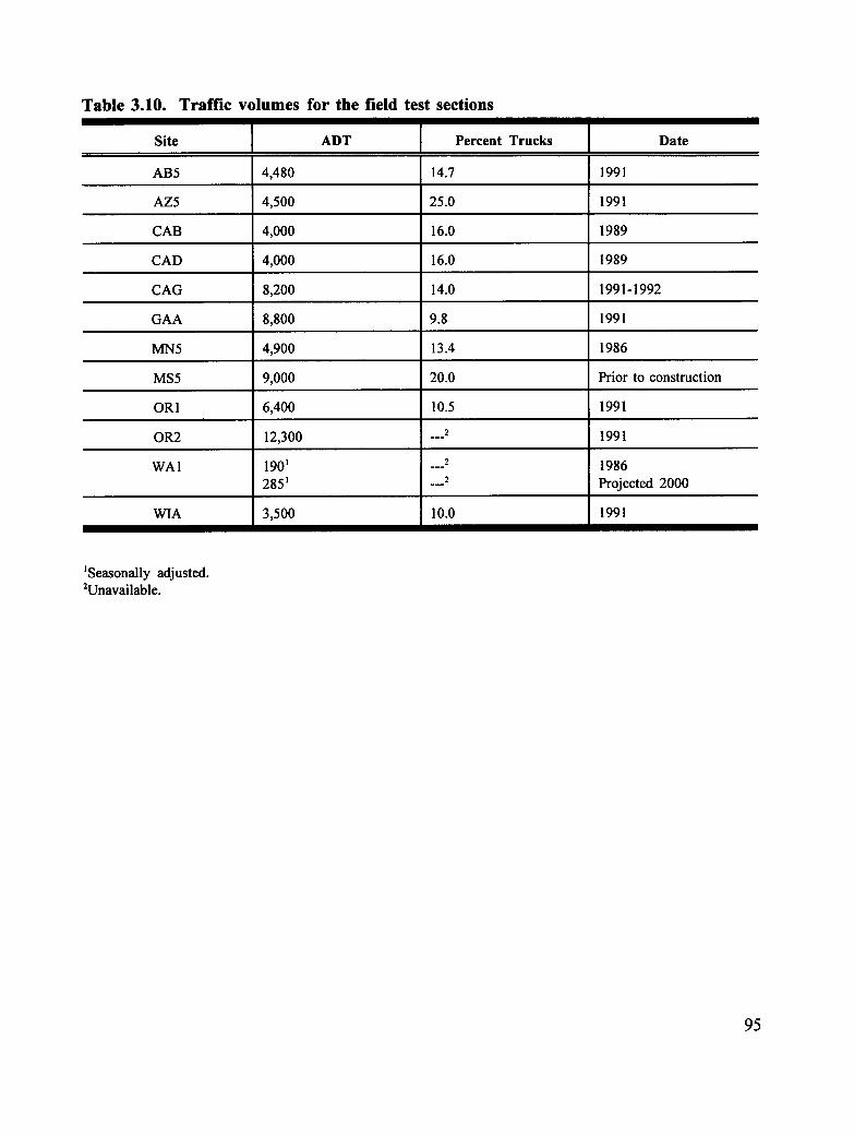
Table 3.10. Traffic volumes for the field test sections
Site ADT Percent Trucks Date
AB5 4,480 14.7 1991
AZ5 4,500 25.0 1991
CAB 4,000 16.0 1989
CAD 4,000 16.0 1989
CAG 8,200 14.0 1991-1992
GAA 8,800 9.8 1991
MN5 4,900 13.4 1986
MS5 9,000 20.0 Prior to construction
OR 1 6,400 10.5 1991
OR2 12,300 .._2 1991
WA1 1901 ._2 1986
2851 .__2 Projected 2000
WIA 3,500 10.0 1991
_Seasonally adjusted.2Unavailable.
95

Table 3.11. ;ummary of pavement condition surve, rs
Site Survey Type Survey Date Comments
AB5 Manual August 92 In good condition, small amount ofcracking
AZ5 Manual August 92 In good condition, some trafficdensification
CAB Manual August 92 In good condition
CAD Manual August 92 In good condition
CAG Manual August 92 In good condition
GAA Covered by wearing course
MN5 Manual June 92 Some low-to-moderate-severity, transversecracking, 5 mm-8 mm rutting, some low-to-moderate-severity bleeding
MS5 Manual In bad condition, reflective cracking,scheduled for overlay
OR1 Covered by wearing course
OR2 Manual 1992 No visual distress with the exception of1/8 in. to 3/8 in. of rutting
WA1 Manual September 92 In good condition, no visible rutting
WIA Manual 1991 In good condition,PDI=0, psi=4.3,1/10 in. of rutting measured
96
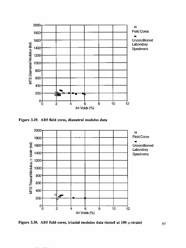
2000 o
1800 FieldCoresI
1600 UnconditionedLaboratory
_ 1400 Specimens'-!
_ 1200'
N lOOO
._a
N 6oo400
200 a_ c =:=.. "_n
00 2 4 6 8 0 12
Air Voids (%)
Figure 3.29. AB5 field cores, diametral modulus data
200(> cz
1800" FieldCoresll
__ 1600" Unconditioned,- Laboratory"_ 1400' Spedmensif)
1200"
" 1000."O0
-_ 800"
•" 600-i--
_m 400-
200" - - :
00 2 4 6 8 10 12
AirVoids (%)
Figure 3.30. AB5 field cores, triaxial modulus data (tested at 100 _t-strain) 97

2000 a
1800 FieldCoresI
1600 Unconditioned'=- Laboratory_'_ 1400 Specimens
"8 1200 ,_m
1000 = -r= -- !800' im
.Na
600.
400'
200'
00 2 4 6 8 10 12
Air Voids (%)
Figure 3.31. AZ5 field cores, diametral modulus data
2000 _ c3
1800 FieldCoresI
.m
1600 Unconditionedv
"1 _ Laboratory._ 1400 Specimens
d 1200u_ Q •
= 1000
-_ 800•_ ,-,_. 600
400.
200'
00 2 4 6 8 10 12
Air Voids (%)
Figure 3.32. AZ5 field cores, triaxial modulus data (tested at 40 psi [275 kPa])
98

2000- oo FieldCores
1800nl-I m
1600" "1 o Unconditionedc Laboratory"[_ 1400 .- Specimens
O ml1:3
d 1200
-_ 1000 '_ :. =
80O
•e" 600'I--
_ 400,
200
00 2 4 6 8 10 12
Air Voids (%)
Figure 3.33. AZ5 field cores, triaxial modulus data (tested at 100 It-strain)
1800" FieldCoresII
1600 UnconditionedLaboratory
1400" SpedmensCt}
1200
_1000 .
_ 800" -l°_
600.
400'
200.
00 2 4 6 8 10 12
AirVoids (%)
Figure 3.34. CAB field cores, diametral modulus data 99

2000" o
1800 FieldCores1::3 n
1600 Unconditionedm Laboratory
1400 _' Spedmens'J 1200 -_._
=3-- m
= 1000 ,=•1_ OO
a-_ 800" o-- o"_ o•,- 600" ,,I-- o t_
400" o
200"
00 2 4 6 8 0 12
Air Voids (%)
Figure 3.35. CAB field cores, triaxiai modulus data (tested at 40 psi (275 kPa))
2000O
.....1800 FieldCores._
n
1600 _ "v
c Unconditioned
•_ 1400 Laboratoryd Specimens
1200
" 1000 " •-o ::_m#:a oO
800" n"_ o" o
.,._ 600" o ..0'' LJI-.-0o 400" o
200"
O0 2 4 6 8 0 12
Air Voids(%)
Figure 3.36. CAB field cores, triaxial modulus data (tested at 100 _t-strain)100

2000- o
1800" FieldCoresm
1600" UnconditionedLaboratory
1400" SpedmensC/)
-_ 1200
"_ 1000(_ m m
[_ 800' r'l _ mm mm
°_ ma
0o,400'
200
00 2 4 6 8 10 12
Air Voids (%)
Figure 3.37. CAD field cores, diametral modulus data
2OOOra ra
1800 -1 FieldCoresm
1600 o UnconditionedLaboratory
1400 Specimens
1200 m
" 10008_:E800' m -- ,.,_o_ "1•_ ,-,•= 600"
u)
_ 400-
200"
C0 2 4 6 8 0 12
AirVoids (%)
Figure 3.38. CAD field cores, triaxial modulus data (tested at 40 psi (275 kPa))101

2000- oFieldCores
180@R
Unconditioned1600" o Laboratoly
_ 1400 Specimensmd 1200 "1cE:::} 1:3 • m" 1000
800' _ "o--
"= 6001-
40o
200
00 2 4 6 8 10 12
Air Voids (%)
Figure 3.39. CAD field cores, triaxial modulus data (tested at 100 [t-strain)
O
1 FieldCores (Set 1)A
FieldCores (Set 2)
Unconditioned_=-, Laboratory"_ Specimens
Eo_0if)b-
DII=|
0 2 4 6 8 10 12Air Voids (%)
Figure 3.40. CAG field cores, diametral modulus data102

2OO0O
1800 FieldCoresm
1600 UnconditionedLaboratory
_ 1400 Specimens
" 1200
E 800am 600I--- •_ n m
mm n
400 = _ _57-, " =200 o []
00 2 4 6 8 10 12
AirVoids (%)
Figure 3.41. GAA field cores, diametral modulus data
2000{:3
1800 FieldCoresm
1600 UnconditionedLaboratory
1400 Specimens
d 1200
1000 m800
_ 600' ,.,m
-400' = o - ,,Q NO
200' "
00 2 4 6 8 10 12
Air Voids (%)
Figure 3.42. GAA field cores, triaxial modulus data (tested at 40 psi (275 kPa)) 103

2000 o
1800 FieldCoresI
°_
1600 UnconditionedLaboratory.=_
_ 1400 Specimensffi
d 1200I
" 1000"OO
.-_ 800
""- 600I'- o
400 m o "_mO I
200
00 2 4 6 8 10 12
Air Voids (%)
Figure 3.43. GAA field cores, triaxial modulus data (tested at 100 It-strain)
2000. o
1800 FieldCoresI
1600- UnconditionedLaboratory
_m 1400" SpecimensI
"_ 1200"0
loo0.
E 800"a
_ 600-
400° -
200- _ _o
00 2 4 6 8 0 12
Air Voids (%)
Figure 3.44. MN5 field cores, diametral modulus data104

2000 o
1800 FieldCoresm
._ 1600 Unconditioned_- Laboratory"._._1400 Specimens
1200
= 1000
-_ 80O°m
"= 600
400o ='_ n°°
200 =o
00 2 4 6 8 10 2
Air Voids (%)
Figure 3.45. MN5 field cores, triaxial modulus data (tested at 100 It-strain)
2OOOO
1800 FieldCoresi
1600 UnconditionedLaboratory"-'1400Spedmens_.=
"a 1200o
•-_ 1000
800121
600
400 ." _-_= -._i_ =i
200
00 2 4 6 8 10 12
AirVoids(%)
Figure 3.46. MS5 field cores, diametral modulus data105
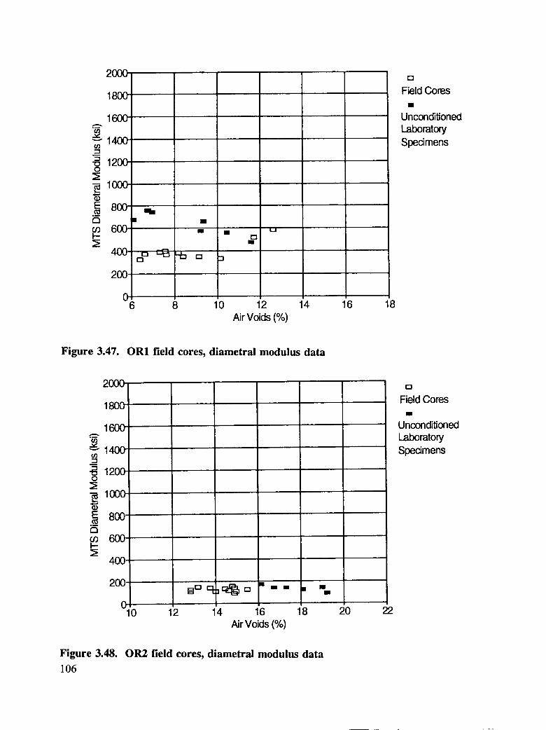
2000 o
1800 FieldCoresi
1600 UnconditionedLaboratory
1400 Specimenst./}
"o 1200o
1000
E 800'(_ liraD m m
600' . ,,
400' _ _----_._ = -_
200'
06 8 10 12 14 16 18
Air Voids (%)
Figure 3.47. OR1 field cores, diametral modulus data
2000- o
1800- FieldCoresIll
1600" UnconditionedLaboratory
1400 SpecimensCt)
-_ 1200-
1000
E 8OO"a
_ 600"
400.
200.B°c_ o - m • mm
010 2 14 16 18 20 22
Air Voids (%)
Figure 3.48. OR2 field cores, diametral modulus data106

20OOI-1
1800 FieldCoresI
1600 Unconditioned
'_- 1400 Laboratory"_ Specimens'm
-_ 1200
"_ 1000
E 800"oua
_ 600.
400.
200" " • •
06 8 10 12 14 6 18
Air Voids (%)
Figure 3.49. WA1 field cores, diametral modulus data
2OOOra
1800 FieldCoresll
1600 Unconditioned"- Laboratory_m 1400 Specimens
-_ 1200
•_ 1000
8oo°_
a
4oo ,,200'
00 2 4 6 8 10 12
Air Voids(%)
Figure 3.50. WIA field cores, diametral modulus data 107

Table 3.12. Visual stripping evaluation of field cores
Specimen Visual Stripping (%)t Comments
AB5F01B 10AB5F12 10
AZ5F03 10 Fines not stripped as inAZ5F09 10 laboratory specimens
CABF02 5CABF10 5
CADF06 0CADF07 5
CAGF01 20 Very similar to laboratoryCAGF 12 20 specimens
GAAF02B 0 Very blackGAAF06A 5
MN5F06 5
MN5 F21 5
MS5F02 5 Much darker than laboratory
MS5F03 5 specimens
OR1F06 0
OR1F09 5
OR2F05 10OR2F12 10
WA1F01 5
WA 1F07 5
WIAF01 5 Asphalt duller than laboratoryWIAF 13 5 specimens
_Evaluated according to Figure 2.20, Visual stripping rating chart.
108

4
Discussion and Analysis of Results
This chapter presents a discussion and analysis of the results obtained from the fieldvalidation effort for water sensitivity. Included is a description of the statistical analysisundertaken on the data from the Environmental Conditioning System (ECS), Oregon StateUniversity (OSU) wheel tracker, Elf Asphalt wheel tracker, and field cores. The analysisincludes ranking of the performance of the mixtures relative to each other in each testformat, development of statistical models for predicting performance of mixtures in eachtest format, and a comparison of the performance of the mixtures by test procedure.Discussion of general relationships of weather and traffic to the pavement performance arealso included.
Analysis of the data obtained during this effort included several goals. First, a ranking ofmixture performance for each test procedure was produced. This ranking was based onsimple models that related the test performance criteria (i.e., ECS modulus ratio, rut depth,and field core modulus ratio) to mixture type only. This allowed for comparison of theranking from each test procedure. Second, statistical models were developed to determinethe importance of such factors as mixture type, air voids, and air and water permeability onthe performance of a mixture in the ECS. Comparison of the effect of test procedures onthe performance of the mixtures was made by comparing the rankings generated, using eachset of test data. Finally, a model of the modulus ratios developed from ECS and field coredata was used to determine the severity of the test procedures relative to one another.
This analysis is designed to demonstrate that the ECS test can discriminate among superiorand inferior asphalt concrete mixtures, as demonstrated by their performance in full-scalefield sections and in the OSU wheel tracker. The analysis of results will also form thebasis for specifications regarding the use of ECS in a mix design system.
ECS Test Results
ECS Modulus Data
The analysis of the ECS test results employed a General Linear Model (GLM) procedure as
109

provided by the SAS software package (SAS Institute Inc. 1988) to rank the mean ECSmodulus ratios (the dependent variable) for each mixture. The performance ranking of themixtures used the T groupings for the mean ECS modulus ratio generated in the GLMprocedure, using the least-significant-difference (LSD) approach. Four rankings wereproduced: (1) a ranking of the ECS modulus ratio for each cycle of the ECS procedure,for the entire data set; (2) a ranking of the ECS modulus ratio for each cycle of the ECSprocedure, for the mixtures from environments with freeze designations; (3) a ranking ofthe ECS modulus ratio for each cycle of the ECS procedure, for mixtures fromenvironments with no-freeze designations; and (4) an overall ranking using the final ECSmodulus ratio obtained for each mixture. For mixtures that came from no-freeze
environments, the final ECS modulus ratio is the ECS modulus ratio after three hot cycles.For mixtures from freeze environments, the final ECS modulus ratio is taken after three hotcycles and the fourth freeze cycle. The ranking using the final ECS modulus ratio isdirectly analogous to the performance of the mixture in its particular environmental zone.
The initial rankings for the purposes of comparison among the test procedures used asphaltmixture type (MIX) type, as a class variable. Tables 4.1 through 4.4 show rankings ofmixture performance in the ECS with the ECS modulus ratio modeled on mixture typeonly. The four cases discussed above are shown. For mixtures MS5 and WIA, onlyspecimens that survived the ECS procedure without excessive deformation were used in theanalysis, which includes three MS5 specimens and five WIA specimens.
The mixtures tested demonstrated two typical responses. Mixtures seem to eitherexperience most of their damage during the first cycle of ECS conditioning and thenmaintain a fairly constant modulus ratio, or continue to decrease in modulus through laterECS cycles, demonstrating continuing water damage. Figures 3.1 through 3.12 illustratethat several of the mixtures experience a high percentage of the reduction in ECS modulusratio in the first cycle of the test. Table 4.5 indicates that eight of the mixtures testedexperienced over 50 percent of their reduction in modulus in the first cycle. This resultindicates that these mixtures are very susceptible to water damage and will probablyexperience water damage early in their lifetimes.
The difference in the slope of the ECS modulus ratio curve between cycle 1 and cycle 3 isalso different for each mixture. Table 4.6 indicates the mean values of slope for the ECS
modulus curve between cycle 1 and cycle 3 for the mixtures tested. These data arepresented graphically in figure 4.1a and 4.lb. The slope is defined as
Slope = (cycle 3 ECS Modulus Ratio - Cycle 1 ECS Modulus Ratio) (4.1)(3-1)
110

4.1. Ranking of mixtures for the ECS test procedure, T intervals and
groupings, entire data set
Cycle 1 Cycle 2
Mean ECS Mean ECSModulus T Modulus
Rank Mixture Ratio Grouping I Mixture Ratio T Grouping
1 GAA 0.952 A GAA 0.932 A
2 OR2 0.903 A OR2 0.916 A, B
3 OR1 0.877 A, B ORI 0.873 A, B
4 AB5 0.875 A, B WA1 0.865 A, B
5 WA1 0.859 A, B AB5 0.813 B, C
6 MN5 0.776 B, C WIA 0.714 C, D
7 WIA 0.748 C, D AZ5 0.708 C, D
8 AZ5 0.742 C, D MN5 0.707 C, D
9 CAB 0.698 C, D CAB 0.674 D
10 MS5 0.690 C, D MS5 0.667 D
11 CAD 0.647 D CAD 0.630 D
12 CAG 0.505 E CAG 0.447 E
Cycle 3 Cycle 4
Mean ECS Mean ECSModulus T Modulus
Rank Mixture Ratio Grouping Mixture Ratio T Grouping
1 GAA 0.937 A OR2 0.916 A
2 OR2 0.904 A WA 1 0.900 A
3 OR1 0.871 A, B WIA 0.768 A
4 WA1 0.838 A, B, C AB5 0.758 B
5 AB5 0.775 C, D, E CAB 0.554 B
6 AZ5 0.720 C, D, E MN5 0.541 C
7 WIA 0.694 D, E, F CAD 0.457 C2
8 CAB 0.654 D, E, F
9 MN5 0.651 D, E, F
10 MS5 0.623 E, F
11 CAD 0.589 F
12 CAG 0.423 G
1Groupings with the same letter designation include means that are not significantly different.
remaining four mixtures were not tested with the freeze cycle.
111

Table 4.2. Ranking of mixtures for the ECS test procedure, T intervals and
groupings, freeze data
Cycle 1 Cycle 2
Mean ECS Mean ECSModulus T Modulus
Rank Mixture Ratio Grouping _ Mixture Ratio T Grouping
1 OR2 0.903 A OR2 0.916 A
2 AB5 0.875 A, B WA1 0.865 A
3 WA1 0.859 A, B AB5 0.813 A, B
4 MN5 0.776 B, C WIA 0.714 B, C
5 WIA 0.748 C, D MN5 0.707 B, C
6 CAB 0.698 C, D CAB 0.674 C
7 CAD 0.647 D CAD 0.630 C
Cycle 3 Cycle 4
Mean ECS Mean ECSModulus T Modulus
Rank Mixture Ratio Grouping Mixture Ratio T Grouping
1 OR2 0.904 A OR2 0.916 A
2 WA 1 0.838 A WA 1 0.900 A
3 AB5 0.775 A, B WIA 0.768 A
4 WIA 0.649 B, C AB5 0.758 B
5 CAB 0.654 B, C CAB 0.554 B
6 MN5 0.651 B, C MN5 0.541 C
7 CAD 0.589 C CAD 0.457 C
Groupings with the same letter designation include means that are not significantly different.
112

Table 4.3. Ranking of mixtures for the ECS test procedure, T intervals and
groupings, no-freeze data
Cycle 1 Cycle 2Rank
Mean ECS Mean ECSModulus T Modulus T
Mixture Ratio Grouping _ Mixture Ratio Grouping
1 GAA 0.952 A GAA 0.932 A
2 OR1 0.877 A OR1 0.873 A
3 AZ5 0.742 B AZ5 0.708 B
4 MS5 0.690 B MS5 0.667 B
5 CAG 0.505 C CAG 0.447 C
Cycle 3
Mean ECS Modulus
Rank Mixture Ratio T Grouping
1 GAA 0.937 A
2 OR1 0.871 A
3 AZ5 0.720 B
4 MS5 0.623 B
5 CAG 0.422 C
_Groupings with the same letter designation include means that are not significantly different.
113

Table 4.4. Ranking of mixtures for the ECS test procedure, T intervals and
groupings, final ECS modulus ratio, regardless of environmental zone
Rank Mixture Mean Ratio T Grouping 1
1 GAA 0.937 A
2 OR2 0.916 A
3 WA 1 0.900 A
4 OR1 0.871 A, B
5 WIA 0.768 B, C
6 AB5 0.758 B, C
7 AZ5 0.720 C, D
8 MS5 0.623 D, E
9 CAB 0.554 E, F
10 MN5 0.541 E, F
11 CAD 0.457 F, G
12 CAG 0.422 G
1Groupings with the same letter designation include means that are not significantly different.
114

Table 4.5. Percent of ECS modulus ratio reduction that occurs in cycle 1
Percentage Final ECS
Cycle 1 Mean ECS Mean Final ECS Modulus Ratio Lost inMixture Modulus Ratio Modulus Ratio Cycle 1
AB5 0.875 0.758 52
AZ5 0.742 0.720 92
CAB 0.698 0.554 68
CAD 0.647 0.457 65
CAG 0.505 0.423 86
GAA 0.952 0.937 76
MN5 0.776 0.541 49
MS5 0.690 0.623 82
OR1 0.877 0.871 95
OR2 0.903 0.916 115
WA1 0.869 0.900 131
WIA 0.748 0.768 109
115

Table 4.6. Mean slope of ECS modulus ratio from cycle 1 to cycle 3
Site Slope
AB5 -0.0498
AZ5 -0.0103
CAB -0.0224
CAD -0.0307
CAG -0.0402
GAA -0.0093
MN5 -0.0290
MS5 -0.0337
OR1 -0.0029
OR2 0.0014
WA1 -0.0115
WIA -0.0125
116

1.20AB5
1.00_L. .j AZ5
o
n" 0.80 _ CAB
-" CAD0.60 __
C/3
_ .--. CAG
"5 0.40 .laGAAt-
0.20
0.0(0 2 3 4
Cyde
Figure 4.1a. Slope of mean ECS modulus ratio curves between cycle 1 and cycle 3
1.201 .4_MN5
1.00 MS5O C'1
tdleq
rr 0.80 . _...._ OR1
---0.60
WA1
0.40-_ WIA=)
0.20
0.000 1 2 3 4
Cycle
Figure 4.lb. Slope of mean ECS modulus ratio curves between cycle 1 and cycle 3117

It is believed that the slope is an indicator of the rate of damage to the specimen as itundergoes the ECS test procedure. Figure 4.2 shows graphically the change in ECSmodulus ratio between cycle 1 and cycle 3. The slopes of the modulus curves betweencycle 1 and cycle 3 indicate that several of the mixtures experience a reduction in modulusratio between cycle 1 and cycle 3 of 0.100 or greater (AB5, CAG, and MN5). Thesemixtures experienced a continual rate of damage and would probably continue toaccumulate damage if subjected to further conditioning. The mixtures that underwent thefourth freeze cycle, (OR2, WA1, and WIA), actually had lower ECS modulus ratios afterthe third cycle than after the final freeze cycle. This is illustrated in figure 4.3.
The model developed using only mixture type as a variable to describe the ECS modulusratio is reported in table 4.7. The values of the probability of F > F0 (0.0001) indicate thesignificance of mixture type to the prediction of the ECS modulus ratio after each cycle.Also note the similar values of R2 and the coefficient of variation after each cycle.
Additional analyses were performed to investigate a more comprehensive set of variables,including percent air voids, air permeability (APERM), initial water permeability(WPERM), and initial ECS modulus. MIX, APERM and WPERM were presented as classvariables in the model. Since both APERM and WPERM measurements resulted in
specimens with reported "zero" permeability values, or permeabilities lower than thecapabilities of the test equipment, these values were divided into four ranges, as shown intable 4.8. The other variables, air voids (AVOID) and initial modulus (INTM), wereanalyzed as covariates (or continuous variables) in the model, using their numeric values.The analyses of the full set of variables was performed on the results after eachconditioning cycle; however, the statistics for cycle 1 will be used to illustrate the selectionof variables significant to the model.
The analysis to investigate the significance of additional variables to the model proceededby adding variables to the model that contained only the variable MIX. If the inclusion ofa variable resulted in significant values of the probability of F > F0 (< 0.05), then thevariable was considered significant. The variable was then added to the model, andpossible interactions of that variable were considered. Table 4.9 indicates the results of thisstudy.
Table 4.9 indicates that the most significant variable after considering MIX is the INTMmodulus of the mixture. None of the other variables have significant probabilities of F > F0when combined with MIX alone to constitute a model. The third variable that can be
added to the model is the AVOID level of the mixture. When added to a model alreadycontaining MIX and INTM, AVOID has a significant value for the probability of F > F0.From the analysis, no other variables, or interactions, add significance to the model, so noother should be included. Therefore, the APERM and WPERM of the unconditionedspecimen do not have a statistically significant effect on the final ECS modulus ratio for themixture.
Tables 4.10 and 4.11 show the full statistical analysis for the two models mentioned above:MIX, INTM; and MIX, INTM, and AVOID. The variables MIX and INTM are much more
118

significant to the model than AVOID in describing the ECS modulus ratio of a mixturespecimen. The values for the probability of F > F0 indicate that throughout the ECS testprocedure, the INTM of the mixture continues to be significant in the prediction of the ECSmodulus ratio.
The increasing value of the probability of F > F0 for AVOID after each ECS cycle indicatesthat as the ECS procedure continues, the initial value of AVOID is no longer as significantin predicting the ECS modulus ratio. This is logical if you consider that as the specimen isundergoing the ECS procedure, the AVOID level is being changed by mechanical changesin the specimen. The specimen is deforming under repeated loading during hot cycles, andthe flow of water within the specimen may be causing binder migration, also changing theAVOID structure. As the test progresses, the initial AVOID level no longer reflects thetrue AVOID structure of the specimen.
Analysis of the data set indicates the relative importance of the INTM of a specimen to itsperformance in the ECS test procedure, which suggests that further discussion of the INTMparameter is warranted.
For the 12 mixtures investigated in ECS, the INTM values ranged from 87.4 ksi (602 MPa)for OR2, the open-graded mixture, to 1,969.3 ksi (13,568.5 MPa) for CAB. Figure 4.4shows the relation between the final ECS modulus ratio and the initial ECS modulus.
Figures 4.5a and 4.5b divide the data by mixture type. For several of the mixtures, theINTM does not vary substantially, such as with AB5, GAA and OR2. However, for othermixtures, the range of initial resilient modulus is quite large, such as with CAD with INTMvalues ranging from 616.8 ksi to 1,709.5 ksi (4,250 MPa to 11,778 MPa).
The INTM of a mixture depends on several factors, such as gradation, aggregate type,aggregate shape, asphalt content and asphalt type, and AVOID. For any particular mixtureused in this task, only AVOID was varied within a set of specimens for the given mixture.Figures 4.6a and 4.6b indicate the relation between INTM and AVOID. (The scales ofthese figures are expanded to accommodate the OR2 open-graded mixture.) This variationindicates that several mixtures experienced significant changes in resilient modulus withchanges in AVOID levels, such as CAB and CAD. For others, OR2 and AB5, the resilientmodulus is less sensitive to AVOID levels.
Though the aggregate for each specimen was batched to the required gradation andconsidered a constant for each mixture, certain asphalt-aggregate mixtures may be verysensitive to relatively minor changes in volumetric properties, such as gradation or asphaltcontent. This sensitivity may also contribute to the wide range of resilient modulus valuesobtained for the CAB and CAD mixtures.
Identifying the initial resilient modulus of a mixture as a variable that influences theperformance of a mixture in ECS requires additional consideration for the purpose ofdefining the relative performance between mixtures. A mixture that has an INTM of 1,000ksi (6,890 MPa) and a final ECS modulus ratio of 0.6 still has a resilient modulus of600 ksi (4,134 MPa). However, a mixture that has an INTM of 667 ksi (4,596 MPa) has tohave a final ECS modulus ratio of only 0.9 to bring it to the same level of resilientmodulus, 600 ksi (4,134 MPa).
119

0 0 o-0
'qr-'-
I u
N _DD< :0 '-'
0
=
.=.
• 0_ d
@4 _1 -- v- ,-
(ww) Ja_loeJJ_laaqM nso 'qldao Inw
120

CO _!"
0 000
N
0
nu _ _=
23 _D "0 u
o _
Z 0 "_o
:_ o wCO J-
121 _
0._ _."
¢,iCXl CXl 'v- _ _.
(ww) Je_ioeJ1IeaqM nso '41dec!lnl=!
121

Table 4.7. GLM analysis of ECS results for mixture type, entire data set
Levels I Values
MIX 12 AB5, AZ5, CAB, CAD, CAG, GAA, MN5,MS5, OR1, OR2, WA1, WIA
Cycle = 1Model: R2 = 0.62, CV = 13.36%, and the ECS modulus ratio mean = 0.781
Degree of Type III Sum of Probability of F >Source of Error Freedom Squares F Values F0
MIX I 1 1.10147487 9.19 0.0001
Cycle = 2Model: R2 = 0.64, CV = 14.84%, and the ECS modulus ratio mean = 0.755
Degree of Type III Sum of Probability of F >Source of Error Freedom Squares F Values F0
MIX 11 1.35601930 9.81 0.0001
Cycle = 3Model: R2 = 0.62, CV = 17.08%, and the ECS modulus ratio mean = 0.733
Degree of Type III Sum of Probability of F >Source of Error Freedom Squares F Values F 0
MIX 11 1.53639193 8.90 0.0001
Cycle = 4Model: R2 = 0.69, CV = 18.12%, and the ECS modulus ratio mean = 0.706
Degree of Type III Sum of Probability of F >Source of Error Freedom Squares F Values Fo
MIX 6 1.38321444 14.10 0.0001
122

Table 4.8. Class variables
Mixture Levels Values
MIX 12 AB5, AZ5, CAB, CAD, CAG, GAA, MN5,MS5, OR1, OR2, WA1, WIA
APERM 4 Very low < 1 E-05 cm/sec.1 E-05 < low < 4 E-05 cm/sec.4 E-05 < medium _<9 E-05 cm/sec.
High > 9 E-05 cm/sec.
WPERM 4 Very low < 5 E-05 cm/sec.5 E-05 < low _<2 E-04 cm/sec.2 E-04 < medium < 5 E-04 cm/sec.
High > 5 E-04 cm/sec.
123

Table 4.9. GLM analysis of ECS results, investigation of significance of variable to themodel
Variable Type
MIX ClassAVOID CovariateINTM CovariateAPERM ClassWPERM Class
Degree of Type 1II Sum of Probability of F >Source of error Freedom Squares F Values F o
MIX 11 1.10147487 9.19 0.0001
MIX 11 1.08011127 9.00 0.0001AVOID I 0.00958422 0.88 0.3525
MIX 11 1.021433805 10.92 0.0001INTM 1 0.15428787 18.14 0.0001
MIX 11 1.06856734 8.99 0.0001APERM 3 0.03752048 1.16 0.3340
MIX 11 1.10473184 9.86 0.0001WPERM 3 0.07353670 2.41 0.0765
MIX II 0.17836491 1.83 0.0742INTM 1 0.00299512 0.34 0.5637
MIX*INTM ll .07588992 0.78 0.6596
MIX 11 1.09239167 13.38 0.0001INTM 1 0.21688027 29.21 0.0001
AVOID 1 0.07219662 9.72 0.0028
MIX I1 0.98883134 10.60 0.0001INTM 1 0.14343805 16.91 0.0001
APERM 3 0.02667066 1.05 0.3784
MIX 11 1.03808863 11.52 0.0001INTM 1 0.12392750 15.12 0.0001
WPERM 3 0.04317633 1.76 0.1658
MIX I1 0.13979178 1.94 0.0571INTM 1 0.23514720 35.91 0.0001
AVOID 1 0.05254372 8.02 0.0067MIX*AVOID 11 0.12372222 1.72 0.0979
MIX 11 1.04396543 12.78 0.0001INTM 1 0.18533145 24.97 0.0001
AVOID 1 0.06784111 9.14 0.0038APERM 3 0.02233515 1.00 0.3984
MIX 11 1.10677529 14.24 0.00011NTM 1 0.16991928 24.06 0.0001
AVOID 1 0.07148224 10.12 0.0024WPERM 3 0.04248196 2.00 0.1237
124

Table 4.10. GLM analysis of ECS results for model I, entire data set
Variable Type Levels Values
MIX Class 12 AB5, AZ5, CAB, CAD,INTM CAG, GAA, MN5,
MS5, OR1, OR2, WA1,WIA
Cycle = IModel: R_ = 0.71, CV = 11.80%, and the ECS modulus ratio mean = 0.781
Degree of Type III Sum of Probability of F >Source of Error Freedom Squares F Values Fo
MIX 11 1.02143805 10.92 0.0001INTM 1 0.15438787 18.14 0.0001
Cycle = 2Model: R2 = 0.73, CV = 12.88%, and the ECS modulus ratio mean = 0.755
Degree of Type III Sum of Probability of F >Source of Error Freedom Squares F Values Fo
MIX 11 1.31219949 13.03 0.0001INTM 1 0.19907440 21.05 0.0001
Cycle = 3Model: R2 = 0.76, CV = 13.71%, and the ECS modulus ratio mean = 0.733
Degree of Type III Sum of Probability of F >Source of Error Freedom Squares F Values Fo
MIX 11 1.60139858 14.40 0.0001INTM 1 0.35085712 34.69 0.0001
Cycle = 4Model: R 2 = 0.79, CV = 15.15%, and the ECS modulus ratio mean = 0.706
Degree of Type III Sum of Probability of F >Source of Error Freedom Squares F Values Fo
MIX 11 0.72009792 10.49 0.0001INTM 1 0.19820338 17.33 0.0001
125

Table 4.11. GLM analysis of ECS results for model II, entire data set
Variable Type Levels Values
MIX Class 12 AB5, AZ5, CAB, CAD, CAG,AVOID Covariate GAA, MN5, MS5, OR1, OR2,INTM Covariate WAI, WIA
Cycle = 1Model: R_ = 0.75, CV = 11.03%, and the ECS modulus ratio mean = 0.781
Degree of Type III Sum of Probability of F >Source of Error Freedom Squares F Values Fo
MIX I 1 1.09239167 13.38 0.0001AVOID I 0.07217662 9.72 0.0028INTM 1 0.21688027 29.21 0.0001
Cycle = 2Model: R2 = 0.75, CV = 12.64%, and the ECS modulus ratio mean = 0.755
Degree of Type III Sum of Probability of F >Source of Error Freedom Squares F Values F 0
MIX 11 1.30335719 13.00 0.0001AVOID 1 0.02966349 3.25 0.0764INTM 1 0.22860297 25.08 0.0001
Cycle = 3Model: R2 = 0.76, CV = 13.64%, and the ECS modulus ratio mean = 0.733
Degree of Type III Sum of Probability of F >Source of Error Freedom Squares F Values Fo
MIX 11 1.55353354 14.10 0.0001AVOID 1 0.01588782 1.59 0.21281NTM 1 0.35459809 35.41 0.0001
Cycle = 4Model: R2 = 0.80, CV = 14.80%, and the ECS modulus ratio mean = 0.706
Degree of Type III Sum of Probability of F >Source of Error Freedom Squares F Values Fo
MIX 11 0.72399953 11.06 0.0001AVOID 1 0.03048498 2.79 0.1033INTM 1 0.22807043 20.90 0.0001
126

80
0.0
m
• L)v
• )
• ._ _'mm ._
• • _ 6.Y')
mUm 0 -mmm ._
m iN m E =
.._• • o
m -" _m 0m_i mml i m._ _=
• ii • m iN l• • •
" ,' °iNiN••m • mm _
• • =
,40 O 0 0 0 0 0
0!I_ snlnpo_ SO3 IEU!=l127

1.20,4k.
AB5A
1.00 "'AZ5
O n A ]i(
=_ =m_ CABrc 0.80 - .- ,=,(n o A
:3 i ql o"_ D CADo:_ 0.60 .. _ '-' Noo N CAGo N QLLI r'l IN-_ 0.40 _'_ A.=_ N N GAALL
I-I r'l
0.20
0.0(0 500 1000 1500 2000
InitialECSModulus(ksi)
Figure 4.5a. Final ECS modulus ratio versus initial ECS modulus, by mixture
1.20i
N MN5
-1.00 m MS5
._o c_::3_ N A N mlrr 0.80 ,-, I_ A _ _ OR1(n N:3 • _ r't--,i
"o • .= • OR,?.o:_ 0.60 •• No WA1ILl I
0.40 At- uE WIA
0.20
0.0(0 500 1000 1500 2000
InitialECSModulus(ksi)
Figure 4.5b. Final ECS modulus ratio versus initial ECS modulus, by mixture128

200OIm i
AB5O Q
._. 1500 AZ5.l
o CABt_ Qo-'! i-i
•_ m " ,A.., CAD1000 m N03 N
O ,., CAGLU"-_ _q' c
_c G_
500 N_ .
£0 5 10 15 20 25
AirVoids (%)
Figure 4.6a. Initial ECS modulus versus air voids, by mixture
2OOOI
MN5ID
.-. 1500 MS5.l
OR1r7
°1000 OR2
03 _ Now WA1
!II
A"C 1 _ WIA
-- 500' -' ,. _ N_--t m I_' N
" 'ill NII 0 O0 f'_
l 0 _I 0
00 5 0 15 20 25
Air Voids(%)
Figure 4.6b. Initial ECS modulus versus air voids, by mixture129

In considering the performance of the two mixtures, their relative levels of stiffness -- notjust the reduction in stiffness as quantified by the resilient modulus ratio -- must beconsidered. Determination of the required level of stiffness for an asphalt-concrete mixturebeing considered for placement is beyond the scope of the water sensitivity task. ECS willindicate the predicted loss of modulus that a given mixture will experience due to waterdamage. It is up to the designer to determine if this will lower the value of a modulus toan unacceptable level.
An additional model was run using a class variable (designated as ENVR) to see if theenvironment, freeze or no-freeze, had a significant effect on the final ECS modulus ratioobtained in the test. Table 4.12 gives the results of this model. The probability of F > F0indicates that the environmental zone does not have a significant effect in the model. TheT grouping of the means for the freeze and no-freeze data also indicate this. Therefore, itcan be concluded for the mixtures tested that neither of the two ECS procedures -- three
hot cycles or three hot cycles plus a fourth freeze cycle -- is statistically more severe.Subjecting a specimen to the appropriate conditioning for its environmental designation willnot influence the performance of the mixture relative to other mixtures tested inconditioning appropriate to their environmental designations. The fact that different gradesof asphalt are typically used for freeze and no-freeze environments may also be reflected bythese data.
Visual Degree of Stripping and Binder Migration Data
The visual degree of stripping and binder migration were not included in the statisticalmodels run on the ECS data. Visual degree of stripping and binder migration, like ECSmodulus ratio, are response variables that change during the ECS test procedure, and it istherefore inappropriate to use them as variables to describe ECS modulus ratio responses.However, some general observations concerning the asphalt stripping and binder migrationdata can be made.
The visual degree of stripping and the binder migration did not seem to have a correlationwith the decrease in modulus as measured by ECS. Several mixtures with low final ECSmodulus ratios have higher degrees of stripping (AZ5, CAG, and MS5); however, somemixtures with lower degrees of stripping also have low final ECS modulus ratios (CAB,CAD and WIA). Binder migration shows similar trends. However, within a set ofspecimens from one mixture, greater binder migration occurs for specimens with lower airvoid levels.
Permeability Data
After 30 minutes of conditioning, some specimens that are impermeable to air allow waterto flow. Additionally, specimens with initial coefficients of permeability for water of lessthan 1.0E-04 crn/sec. (3.9E-05 in./sec.) typically show an increase in permeability duringthe first hot cycle with repeated loading. This suggests that the wetting procedure and,even more so, the heating and loading procedure of the first hot cycle with available flow,tend to open the specimen to flow. Several mechanisms may be at work.
130
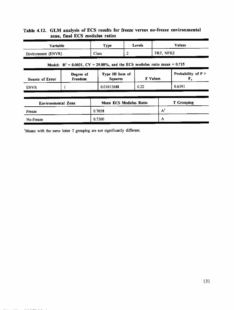
Table 4.12. GLM analysis of ECS results for freeze versus no-freeze environmental
zone, final ECS modulus ratios
Variable Type Levels Values
Environment (ENVR) Class 2 FRZ, NFRZ
Model: R2 = 0.0031, CV = 29.88%, and the ECS modulus ratio mean = 0.715
Degree of Type III Sum of Probability of F >Source of Error Freedom Squares F Values Fo
ENVR 1 0.01012688 0.22 0.6391
Environmental Zone ] Mean ECS Modulus Ratio ] T Grouping
Freeze [ 0.7058 [ A _No-Freeze 0.7300 A
_Means with the same letter T grouping are not significantly different.
131

During the wetting procedure, the extended time with 20 in. (508 ram) Hg vacuum pressuremay allow water to break through thin films of asphalt that may separate voids in thespecimen. The 30-minute period may be why this break occurs with water flow during thewetting procedure and not during the air flow measurements. In the air permeability test,the air flow is immediately turned off if the specimen is deemed impermeable, so thepressure differential does not last for more than a few minutes.
During the first cycle of loading, specimens with lower coefficients of water permeabilitymay see more breakdown of thin films that separate voids. The repeated loading may causerearrangement of the asphalt-aggregate matrix and breaking of the asphalt bonds. Also,repeated loading may cause increased pore water pressure within the specimen, especially ifwater is trapped in pores with only one interconnecting pathway to other pores, or ifpathways between pores are small, causing more film damage. During the first cycle,specimens may also be experiencing a loss of adhesion within the asphalt matrix. Severalof the specimens that tended to show an increase in permeability during the first cycle werealso the specimens in which more binder migration was observed.
Figures 3.15 through 3.36 indicate that within a group of specimens from one mixture, thespecimens with lower air voids tend to have lower coefficients of water permeability. Thisis also seen in figure 3.14. During the first cycle of ECS testing, the less porous specimensshow increasing coefficients of water permeability. More permeable specimens tend toshow a decrease in permeability during the first cycle. The lower permeability specimenshave visual stripping similar to the more permeable specimens of the mix; however, theytend to show higher levels of binder migration than the other specimens of the mixture.This trend is true for all the mixtures that had specimens that displayed binder migration(AB5, AZ5, CAB, CAG, MN5, MS5, OR1, and WA1).
It may be that lower permeability specimens with lower air void levels present a matrixwith thicker asphalt films and less interconnection between pores. Under the action ofwater flow and repeated loading, higher pore water pressures may tend to break these filmsand move debonded asphalt particles around until an equilibrium is reached and the poresare connected in such a way as to provide adequate drainage for the structure under theprevailing conditions. In the more permeable mixtures with higher air void levels, theexisting pathways between pores may be adequate and pore water pressures may not be aslarge under the actions of repeated loading.
During the second, third, and fourth cycles, specimens of all air void levels andpermeabilities tend to show either very little variation in permeability or a continualdecrease in the coefficient of water permeability. This is probably due to the deformationof the specimen under repeated loading. This would tend to decrease the air void contentof the specimen and create a structure of smaller pores separated by a dense asphalt-aggregate matrix. Typically, the fourth freeze cycle does not vary this trend.
132

OSU Wheel Tracker Results
A ranking of the mixtures as they performed in the OSU wheel tracker is presented intable 4.13. This ranking was again produced using the GLM procedure, and the resulting Tintervals. The model included only MIX as a class variable. The dependent variable is rutdepth, designated by a negative number. A second model including the covariate AVOIDwas also produced. This model is presented in table 4.14.
When interpreting the results of the OSU wheel tracking tests, it is important to comparethe air void levels of the beam specimens with the kneading-compacted specimens tested inECS and the cores taken from the field. Because of the limited amount of material
available for preparing specimens, only two beams were prepared for each mixture. Ifproblems occurred during the specimen manufacturing process, additional specimens couldnot be fabricated. For example, the MN5 mixture was very difficult to compact, and asignificant portion of the mixture was lost because of adhesion to the drums of the roller.Therefore, MN5 beams had significantly different air voids than intended. Table 4.15compares the average air void levels of the different specimens.
Table 4.16 presents the mean modulus ratios for the rutted beam specimens. Two methodswere used to calculate initial modulus values for these specimens. First, the simple averageof the diametral modulus of the unconditioned cores taken from the OSU wheel tracker slab
was used. Second, a relation for diametral modulus values for the unconditioned roller-compacted slab cores and air voids was developed using simple linear regression, and the airvoid level of the rutted core was used to calculate a corresponding initial modulus. Sincethe rutted cores typically have lower air void levels than the unconditioned companioncores, using either method is prone to error, as it is an extrapolation outside the range of theinitial air void data. Additionally, the unconditioned cores do not have a large enoughrange in air voids to create a good correlation between diametral modulus and air voids.
Cores from several of the mixtures show very high mean modulus ratios. This is believedto be attributable to the configuration of the test beam in the OSU wheel tracker. Thebeam is confined in such a way as to produce an area of higher density under the wheelpath. This densification of the mixture tends to increase the modulus of the mixture,obscuring any reduction in modulus the specimen may have undergone because of waterdamage to the mixture.
Elf Wheel Tracker Results
Using the rut depth at 5,000 wheel passes, as with the OSU wheel tracking data, themixtures tested by Elf have performed as shown in table 4.17. It is interesting to note thatin all cases in which specimens of the same mixture were tested at two differenttemperatures, 40°C and 50°C (104°F and 122°F), the specimen tested at the highertemperature experienced higher rut depths, as expected.
Also, according to the Elf criteria, the WIAELF02 specimen did not experience stripping;however, it reached 18 mm of rutting in 3,000 wheel passes. This behavior is similar tothat of the mixture in ECS, in which it experienced excessive deformation under repeatedloading during the "hot" conditioning cycle.
133

_ _ m _ _ _
o o o < < o :_
____i__ ._
"- _ _ _ <
0
_ _ ....
•_ _
_ _ "_
. { -_ ___ _
1111111111111__o_
134

Table 4.14. GLM analysis of OSU wheel tracker data
Variable Type Levels Values
MIX Class 11 AB5, AZ5, CAB, CAD, CAG,AVOID Covariate GAA, MN5, MS5, OR1, OR2,
WA1, WIA
Passes = 200
Model: R2 = 0.87, CV = -45.09%, and the mean rut depth = -1.324
Degree of Type III Sum of Probability of F >Source of Error Freedom Squares F Values Fo
MIX 10 10.02143661 2.81 0.0676AVOID 1 1.83446358 5.15 0.0494
Passes = 5,000Model: R2 -- 0.98, CV = -16.03%, and the mean rut depth = -6.616
Degree of Type III Sum of Probability of F >Source of Error Freedom Squares F Values Fo
MIX 10 382.0277075 37.73 0.0001AVOID 1 6.44399000 5.735 0.0436
Passes = 10,000Model: R2 = 0.99, CV = -7.24%, and the mean rut depth = -7.137
Degree of Type III Sum of Probability of F >Source of Error Freedom Squares F Values Fo
MIX 10 124.3197927 58.20 0.0001AVOID 1 0.1259595 0.47 0.5143
135

Table 4.15. Average air void levels of test specimens, beams and field cores
ECS Kneading- Field Core,Compacted OSU Wheel Field Core, BetweenSpecimen Tracker Beam Wheel Path Wheel Path
Site (%) (%) (%) (%)
AB5 3.9 6.5 1.4 ! .4
AZ5 7.2 8.4 4.4 4.9
CAB 5.3 No beams 5.4 5.6
CAD 8.3 9.7 6.1 5.6
CAG 8.2 12.0 5.3 6.1
GAA 8.2 7.8 8. I 8.1
MN5 4.9 11.4 4.7 6.5
MS5 6.9 8.3 4.7 6.3
OR1 8.4 8.4 11.8 13.0
OR2 17.8 21.8 13.8 15.0
WA 1 9.5 6.3 7.7 9.4
WIA 1.0 4.1 3.9 4.05
136

Table 4.16. Mean MTS diametral modulus ratios for rutted beam cores
Ratio Based on Mean Initial Ratio Based on RegressedMixture Core Modulus Initial Core Modulus
AB5 0.93 0.80
AZ5 0.89 0.70
CAD 0.47 0.97
CAG 1.43 1.11
GAA 1.02 1.32
MN5 1.88 1.32
MS5 0.86 0.91
ORI 0.76 0.73
OR2 0.66 0.62
WA 1 0.83 0.74
WIA 0.88 2.00I
137
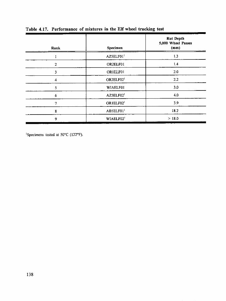
Table 4.17. Performance of mixtures in the Elf wheel tracking test
Rut Depth5,000 Wheel Passes
Rank Specimen (mm)
1 AZ5ELF011 1.3
2 OR2ELF01 1.4
3 ORIELF01 2.0
4 OR2ELF021 2.2
5 WIAELF01 3.0
6 AZ5ELF021 4.0
7 ORIELF021 3.9
8 AB 5ELF011 18.2
9 WIAELF02 _ > 18.0
_Specimens tested at 50°C (122°F).
138

Field Data
Weather Data
Tables 4.18 and 4.19 indicate the variation from the 30-year normals of the precipitationand temperature data for 1991. The 30-year normals perhaps better indicate the climateconditions to be expected over the life of the pavement, rather than any one year of data,because extremes in temperature and precipitation will be averaged from the 30-year data.
It should be kept in mind that even though these sites nominally come from only fourenvironmental zones, the differences in the climate conditions can still be quite significant.For the five sites designated as dry, the 30-year average annual normal precipitation variedfrom 2.71 in. to 22.35 in. (68.8 mm to 567.7 mm). For the six sites designated as wet, the30-year average annual normal precipitation varied from 8.57 in. to 58.09 in. (217.7 mm to1475.5 mm). Variation of precipitation in a given calendar year may be even greater.
Temperature data show similar variation in freeze and no-freeze zones. For sites withfreeze designations, the 30-year average monthly normal temperature varies with lows from2.3°F to 32.1°F (-16.5°C to 0.1°C) and highs from 58.6°F to 70.8°F (14.8°C to 21.6°C).For no-freeze sites, the lows vary from 34.9°F to 54.4°F (1.6 to 12.4°C) and the highs from67.8°F to 91.3°F (19.9°C to 32.9°C).
It is evident that mixtures in the field are subject to a variety of temperature and waterconditions.
Traffic Data
The traffic data obtained for the test sections used in this program were presented in table3.9. The average daily traffic ranged from a low of approximately 190 to a high of 12,300.The percentage of trucks on these pavements ranged from 10 percent to 25 percent. It isevident that traffic volumes varied substantially among test sections.
Field Core Data
Figures 3.29 through 3.50 indicate that for several of the mixtures, the modulus valuesmeasured for the field cores were equal to or greater than the modulus values for new,unconditioned, laboratory-fabricated specimens. For both the MTS diametral and triaxialmodulus data all the mixtures tested had one or more field cores that were equal in stiffnessto unconditioned laboratory specimens. These data indicate that the typical field core takenhas not experienced any decrease in mixture stiffness that would be the result of waterdamage. However, long-term aging may be causing an increase in stiffness in fieldmixtures, and the mixtures as constructed in the field may have varied substantially instiffness from the corresponding laboratory-fabricated specimens.
139

• r_ _ • • c:_
o_
_ o
°_ i._
°_ _ "_
+ �,, + _ _ _om 0
140

,:5 _I _, _, + + + + + + +
_'I _'7 �,"r
r_
t._
._ , , , + + + m,'-7 _ +o_
_ °_
[. d,
141

The general performance indicator for field cores was a ratio of the MTS diametralmodulus of the field core to the MTS diametral modulus of a corresponding unconditionedlaboratory, manufactured specimen. A direct ratio of conditioned field core modulus tounconditioned field core modulus could not be calculated because no cores were taken
immediately after construction to represent the unconditioned case. A linear regressionequation with the MTS diametral modulus as a function of air voids was developed foreach mixture, using the unconditioned, kneading-compacted specimens. This equation wasthen used to predict a corresponding initial MTS diametral modulus value for anunconditioned field core, using the current air void level of each individual core.
For field cores nominally 4 in. (101.6 mm) in height, a similar ratio of MTS triaxialmodulus ratio was also used to compare field core performance directly to performance ofthe mixtures in ECS. An initial unconditioned MTS triaxial modulus value for theunconditioned field cores was calculated in the same manner as for the unconditioned MTSdiametral modulus.
The GLM ranking for the field specimens on the basis of retained MTS diametral modulusratios is presented in table 4.20. The model again had only MIX as an independentvariable. As of 1992, only one field site had deteriorated significantly. MS5 is currentlyscheduled to be overlaid. This mixture is suspected to be water sensitive; however,difficulties during construction may also have produced a lower quality mixture in the field.
Some of the field mixtures have diametral modulus ratios of >1 (WIA AZ5, MS5, andWA1). This may indicate that the mixture has undergone some degree of long-term agingin the field since its placement. Long-term aging tends to increase the modulus of asphaltmixtures.
Comparison of Test Results
Table 4.21 indicates the performance ranking orders given for the mixtures tested in thethree procedures. For ECS, this ranking is based on the final ECS modulus ratio using all12 mixtures, regardless of environmental zone. This listing would correspond to therankings given by the OSU wheel tracker, which uses both freeze and no-freezeconditioning, and to the field, which may present either a freeze or no-freeze environment.
ECS and Field Results
A comparison was made of the performance of the mixtures in the ECS test procedure withtheir performance under field conditions. Field cores tall enough to allow for MTS triaxialmodulus testing were directly compared with ECS specimens by using the laboratoryspecimen MTS triaxial data to correspond with ECS data to produce initial MTS triaxialmodulus data for the field cores. This allowed a modulus ratio to be developed. Sixmixtures were evaluated in this manner. For mixtures placed in layers that did not produce4-in. (101.6 mm) cores, the correlation between the performance of the field mixtures, asmeasured by a diametral modulus ratio, and the performance in ECS, as measured by theECS modulus ratio, was investigated.
142

Table 4.20. Ranking of mixtures for field cores, based on MTS diametral modulusratios
Ranking Mixture Mean Modulus Ratio T Grouping 1
1 WIA 1.192 A
2 AZ5 1.089 B
3 MS5 1.087 B
4 WA 1 1.072 B
5 CAG2 0.848 C
6 MN5 0.821 C
7 OR1 0.716 D
8 CAB 0.715 D, E
9 CAD 0.680 D, E
10 GAA 0.667 D, E
11 OR2 0.642 E, F
12 AB5 0.573 F
_Groupings with the same letter designation include means that are not significantly different.2First set of CAG cores.
143

Table 4.21. Comparison of ranking of mixtures by test method
OSU
Tracking,5,000 Wheel
ECS Passes Field Cores
T
Ranking Mixture Grouping t Mixture T Grouping Mixture T Grouping
1 GAA A GAA A WIA A
2 OR2 A WA1 A, B AZ5 B
3 WAI A CAD A, B, C MS5 B
4 OR1 A, B WIA B, C, D WA1 B
5 WIA B, C OR1 B, C, D CAG C
6 AB5 B, C AZ5 C, D MN5 C
7 AZ5 C, D AB5 D, E OR1 D
8 MS5 D, E MS5 E CAB D, E
9 CAB E, F OR2 E CAD D, E
10 MN5 E, F CAG F GAA D, E
11 CAD F, G MN5 Failed OR2 E, F
12 CAG G AB5 F
_Groupings with the same letter designation include means that are not significantly different.
144
A model was run using the GLM procedure to compare the final ECS modulus ratios withthe field core MTS triaxial modulus ratios. MIX and test procedure (TEST) were theindependent variables. The interaction between the two variables was also included(MIX*TEST).
Table 4.22 shows the results of this comparison. The significant variable according to theprobability of F > F0 is TEST. Table 4.23 indicates the values of the mean modulus ratioand standard deviation for each mixture for each test procedure. For five of the sixmixtures, ECS gives a lower modulus ratio, indicating that the specimens had been moreseverely damaged than the field core. For the sixth mixture, ECS and field mean, MTStriaxial modulus ratios are within one standard deviation of each other.
A comparison of the performance of the mixtures in the ECS and in the field can also beseen in figure 4.7. The MTS diametral modulus ratio of the field cores versus the finalECS modulus ratio is shown. Final ECS modulus ratios are lower than the MTS dimetralmodulus ratios obtained from the field cores for 8 of the 12 mixtures tested. This indicatesthat ECS is predicting more water damage for these mixtures than has yet been experiencedin the field. The effects of aging, variation in precipitation and temperature conditionsamong sites, and the relatively short period of time the mixtures have been in place areprobably responsible. From the most recent field distress surveys, it is known that the MS5field section is showing signs of rutting and reflective cracking, and is due to be overlaid.This distress developed over the 1991-1992 winter season, after the field cores had beentaken in the summer of 1991. At that time, the section showed no signs of distress. MS5is the only field section that at this time shows any substantial distress. For the other fourmixtures (AB5, OR1, OR2, and GAA), ECS predicts no high loss in stiffness caused bywater damage and, to date, the field specimens reflect this behavior.
As mentioned above, when comparing results of the ECS testing with modulus ratiosdeveloped for the field cores, consider the potential for the mixtures in the field toexperience long-term aging. The mixtures tested in ECS are subjected to only short-termaging of the loose mixture. In the field, mixtures are experiencing long-term aging, whichtends to increase the modulus of the mixture. In the early life of the pavement, beforewater damage has developed fully, the increase in stiffness caused by aging may overwhelmany decrease in stiffness that is beginning to occur because of water damage. The datafrom CAG may illustrate this point. In figure 4.7, two sets of cores from CAG arerepresented. CAG 1 represents cores that were taken within one month of paving. CAG 2represents cores taken approximately one year after paving. This mixture has experiencedan increase in MTS diametral modulus over the initial year of pavement life.
Figure 4.8 shows the relationship between the visual stripping shown in field cores and thatobserved in ECS specimens. Typically, specimens from the same mixture appeared verysimilar for the field cores and the ECS specimens. However, two differences were noted:(1) asphalt in the field cores appeared a much duller, fiat black color, while that in the ECSspecimens was typically a dark, shiny black; and (2) no migration of asphalt binder wasseen in any of the field cores. The differences in the appearance of the asphalt betweenfield and ECS specimens may be due to aging of the asphalt in the field. The lack ofmigration of asphalt binder in field specimens may be due to their relatively short lifetimein the field.
145

Table 4.22. GLM analysis of ECS and field core data by test method
Variable Type Levels Values
MIX Class 6 AB5, AZ5, CAB, CAD, GAA, MN5TEST Class 2 ECS, FLD
Model: R 2 = 0.3139, CV = 49.57%, and the modulus ratio mean - 0.972
Degree of Type III Sum of Probability of F >Source of Error Freedom Squares F Values F0
MIX 5 1.27943922 1.10 0.3652TEST I 4.51212952 19.43 0.0001MIX*TEST 5 2.19456568 1.89 0.1039
146

Table 4.23. GLM mean modulus ratio values by test method for each mixture
ECS Field
Mixture Type Mean ECS Standard Mean Triaxial StandardModulus Ratio Deviation Modulus Ratio Deviation
AB5 0.778 0.136 0.768 0.102
AZ5 0.720 0.041 1.205 0.644
CAB 0.554 0.191 1.043 0.557
CAD 0.457 0.155 1.055 0.713
GAA 0.937 0.158 1.099 0.453
MN5 0.541 0.117 1.533 0.581
147

LO_04
(::1)
0-E o8== o
m c_ _ 00• • rr ,- _ ._o
m rr
_ rr _0 5
mr m d_< _ _
m iii _
_m _ _ ,-Z r-- _._ m _ -_
m__m 00 0 *
e_o
0
,-- -- d d o _.
o!leEIsnlnpolAIleJlewe!C]e_oo ple!-I
148

0o'2
V r_
Cr_r- ._.i
i
o
Z rr o0
ml II • _.< o .P
0
0 •
0 ,_.C_ _
CO 04 _I&G
(%) 6u!dd!JlSlens!Aple!-I
149

Currently, there is no correlation between the amount of field life that the ECS proceduresimulates, using either three hot cycles or three hot cycles and one freeze cycle, and thewater damage in the field. ECS indicates that a mixture will experience a certain decreasein modulus and a certain level of asphalt stripping and binder migration but gives noindication of the length of time it will take for this damage to be manifested in the field.Continued monitoring of the mixtures studied in this program will help establish acorrelation between performance in the ECS test procedure and expected field life withrespect to water sensitivity.
ECS and OSU Wheel Tracker
Figure 4.9 shows the relation between the final ECS modulus ratio and the OSU wheeltracker rut depth. The beams manufactured from the MN5 mixture had air voids over200 percent of those found in the ECS kneading-compacted specimens, as shown intable 4.15. If the data points are removed, for MN5, on the basis of its high air voids, andfor OR2, since it is an open-graded mixture, figure 4.10 results. There is no valid reason toremove the data point for CAD from the analysis, even though it represents data from onlyone beam. A best fit line can be placed through these data using simple linear regression,as shown in figure 4.10. With the exception of the mixtures from California, the data fitthis line well.
The correlation of performance is more evident between the ECS data and the OSU wheeltracker data than between the ECS and field core data because ECS and OSU wheel tracker
specimens were under laboratory control and received analogous preparation and water andtemperature conditioning. Specimens from the field do not undergo such well-defined oruniform treatment as is evidenced by the weather and traffic data presented previously.Construction problems may also affect the quality of the pavement placed in the field.Table 2.5 indicates that two projects, MS5 and OR1, experienced problems duringconstruction.
ECS and Elf Wheel Tracker
Figure 4.11 shows the relation between the final ECS modulus ratio and both the OSUwheel tracker and Elf wheel tracker data. The Elf data are similar to those from the OSU
wheel tracker and include only those specimens tested at 40°C (109°F). Variation can beattributed to different mixing and saturation techniques.
150

00
n- rj0 •
I.,..
0
od_
_, "_ _ _
0 _
. C _d _
0
r_
(5 121 ,,o
0 _e_
I O o
_1 _ _-- _ .
(ww) Je_IOmlleeqM n9o '41de(]lnl=l ._o_
151

O-O
0m o
•."<
ix') _m
s =_ E'< :
:m _ _.."w. z.I
; (J ._; I.IJ "_
: d oI; "m
I o
, • ,,:c ".-.::c ; c.) _'Q) ; e.
ol • O. ',_l-
m o m o m od¢kl _ T-- "4
(ww)JeHool laa4AANSO'41decIIn_ ._
152

00
m
_m o 00
d
03 [] _
H.! _ _r_
COI _ O z.
.r,.Omm I"- _d cD '_
(D 0 _• m -_
_ _ _ _ c_c_
(row) qlde(] lnl::!
153

Significance of Findings
From the preceding analysis, several significant findings have emerged. They aresummarized as follows:
ECS results
1. A high percentage of the reduction in ECS modulus ratio occurs in the first cycle ofECS conditioning; however, a significant change may occur between cycle 1 andcycle 3 for some mixtures (MN5, AB5, and CAG).
2. Some mixtures may experience an increase in modulus ratio after the fourth, orfreeze, cycle.
3. The slope of the ECS modulus ratio curve indicates the rate of water damage to thespecimen. At this time, a correlation between cycles of ECS conditioning and thecorresponding period of field life has not been established.
4. Of the variables considered (mixture type [MIX], air voids [AVOID], initial modulus[INTM], air permeability [APERM] and water permeability [WPERM]), the firstthree have the strongest influence on the final ECS modulus ratio of the mixture.
5. There is no statistical difference between the results from mixtures that were
subjected to the freezing cycle and those subjected to only three hot conditioningcycles. This indicates that neither procedure -- three cycles with no freeze, or fourcycles including a freeze -- is consistently more severe. Therefore, subjecting aspecimen to the appropriate conditioning for its environmental designation will notinfluence the performance of the mixture relative to other mixtures tested, usingconditioning appropriate to their environmental designations.
OSU wheel tracker results
1. The air void levels between the beam specimens and the corresponding laboratorykneading compactor specimens vary for some mixtures and may result in high rutvalues (MN5) that are not indicative of the expected performance of the mixture.
2. Anomalous results indicate that several of the mixtures should be retested in this
apparatus (CAD, CAG, and MN5).
Elf wheel tracker results
1. The specimens tested at a higher temperature tend to show increased rutting.
154

Field data
1. Weather data taken from a single observation year may not represent the normalenvironmental conditions that a pavement will be subjected to throughout its life.
2. Within a given environmental zone, temperature and precipitation values may varysignificantly.
3. Traffic volumes will vary substantially, as they did among field projects.
4. Long-term aging of mixtures in the field may increase the modulus of field cores,overshadowing the effects of water damage.
Comparison of test procedures
1. ECS and field cores For mixtures with 4-in.-high (101.6 mm) cores, a comparisonof triaxial modulus ratios indicates that ECS tends to induce more water damagethan field conditions; however, the difference is not statistically significant.
2. ECS and field cores: In a comparison of the final ECS modulus ratio with the fieldcore diametral modulus ratio, ECS predicts more damage than has been experiencedby the field cores for 8 of the 12 mixtures tested. ECS is predicting damage that hasnot yet occurred because of the relative youth of the field sections.
3. ECS and field cores The mixtures in the field may be experiencing long-term aging,which is not simulated in the ECS test procedure.
4. ECS and field cores The field cores have experienced a range of precipitation,temperature, and traffic conditions that is not seen in the ECS testing. All ECSspecimens are tested under the same procedure according to their environmentaldesignation. This will affect the correlation between performance of a mixture inECS and in the field.
5. ECS and OSU wheel tracker A strong correlation between the performance ofmixtures in ECS and the OSU wheel tracker is evident.
6. OSU wheel tracker and Elf wheel tracker Data from the Elf wheel tracker is similar
to that of the OSU wheel tracker for those mixtures tested at 40°C (104°F). Therelationship between the ECS and Elf data is also very good.
155

5
Guidelines for Specifications
It is the goal of the A-003A SHRP task to incorporate the findings of the EnvironmentalConditioning System (ECS) study into usable specifications for one or more levels of mixdesign procedures. The ECS procedure will investigate the susceptibility asphalt mixturesto water sensitivity and determine if a mixture can be expected to perform well with regardto water damage or if the mixture should be redesigned, aggregate or asphalt changes made,or modifiers added.
Three levels of mix design are being considered in the proposed SHRP mix designprogram: level 1, low-volume roads; level 2, intermediate-traffic-volume roads, secondaryroutes; and level 3, primary state routes, high-speed and high-volume roads.
Mixture Properties
As designed in the laboratory, mixtures selected in the preliminary volumetric mix designwill be subjected to short-term oven aging before compaction into specimens for ECS. Thepreliminary mixture design will determine the aggregate and asphalt type to be used and theaggregate gradation and asphalt content.
ECS specimens will then be compacted at two air void levels; 7 percent + 1 percent forlevels 1, 2, and 3, and additional specimens at 10 percent + 1 percent for levels 2 and 3.These air void levels were chosen in accordance with the pessimum voids theory proposedby Terrel and A1-Swailmi (1992). Two specimens will be compacted at each level.
ECS Criteria
Two specimens of a given mixture and of equal air void levels, will be subjected to theECS procedure using three or four cycles; the fourth, or freeze, cycle is optional for use inenvironments that experience freeze-thaw conditions. A plot of the ECS modulus ratioversus cycles will be used to rate the specimen performance.
From the data, a final ECS modulus ratio of 0.7 appears to separate mixtures thatperformed well in the ECS, OSU wheel tracker, and the field from those that showeddeterioration in the OSU wheel tracker or the field. This result is illustrated in figures 5.1and 5.2.
157

80
n- 0 •if)
0 _UJ 0 0 I"
L.I_'_ mE ,,_d a "_ ;
m g
m _
G,I
CXl 04 ',- '!- ,_
(ww) Je_iOeJllaeqM nso 'qldea lnl::l
158

.t'_J
.o
rr"or)
_ O
8_
m mmm mm_ iT _ om rr _
......m._ _ d =..................................8_ UJ .)
mm iT
,- • __ o d _
"r-,oW,.¢
oJm.r) O u') O _O
o!lel=lsnlnpolAIleJ_ewe!aeJoople!=I
159

In using a final ECS modulus ratio of 0.7 to differentiate between acceptable andunacceptable asphalt-concrete mixtures in terms of water sensitivity, it should be noted thatthe change in ECS modulus ratio that occurs between cycle 1 and cycle 3 (as shown infigure 4.2) moved two of the mixtures tested, MN5 and MSS, from acceptable orquestionable to unacceptable. The change in ECS modulus ratio between cycle 3 and cycle4, as shown in figure 4.3, moved the mixture WIA from unacceptable to acceptable.Therefore, when setting criteria for performance of mixtures in ECS, the mixtures beingevaluated should be subjected to the full ECS procedure appropriate for their environmentaldesignation.
It is recommended that the following procedures be used:
• Level 1 If the final ECS modulus ratio is < 0.7, the mixture should be treated formoisture susceptibility, and the treated mixture retested in ECS. If the final ECS modulusratio is < 0.8, the slope of the curve, between cycles 1 and 3, should be investigated. Formixtures with flat slopes, the mixture is expected to perform well and no treatment isrecommended. For mixtures with steeper slopes, treatment of the mixture for moisturesensitivity should be considered because these mixtures may experience significant waterdamage, only at a slower rate than those with final ECS modulus ratios of <0.7.
• Level 2 For mixture specimens with air void contents of 7 percent __1 percent, thecriterion is the same as in level 1. For the specimens with air void content of 10 percent +1 percent, the mixture should be treated for moisture susceptibility if the final ECS modulusratio is < 0.6. Again, the slope of the curve between cycle 1 and 3 is an indicator ofdelayed moisture damage to the mixture.
• Level 3 Level 3 varies from level 2 only in the use of additional tests on the specimensafter the ECS test procedure. Simple shear tests will be performed on both conditioned andunconditioned ECS test specimens, with a requirement for acceptability of the mixture asshown in figure 5.3. If the mixture does not meet the simple shear criteria, it will beredesigned to improve its performance.
Expected Benefits
Evaluation of mixtures with the ECS test procedure should eliminate the placement ofmixtures that could experience water damage within the first several years of life.Currently, only one of the mixtures (MS5) tested in the effort has failed in the field. Thismixture had a final ECS modulus ratio of 0.62 and a slope of-0.0337. Treatment ofmixtures that show tendencies for water damage over a longer life, as evidenced by steepmodulus ratio curves between the first and third cycles, may also be advisable to extendpavement life even further.
160

Conditioned
( p)con
I
I Unconditioned/
Yp (Yp)uc I /
Ndesign
@ Ndesign: (Tp)con/(Yp)uc < 2- 3
Figure 5.3. Simple shear criteria
161

6
Conclusions and Recommendations
The work performed during field validation of the Environmental Conditiong System (ECS)test procedure can be considered as an initial database for correlating the performance ofmixtures in field, in ECS, and in the OSU wheel tracker. The limited amount of materialsavailable, and length of time that pavements have been in the field indicate that additionaltime and testing will only better define the role of ECS in modem mix design.
Conclusions
The following conclusions can be drawn from the data collected in the field validation ofthe ECS test procedure:
1. ECS can discriminate among mixtures that will perform well and those that willperform poorly with regard to water sensitivity of the asphalt mixture.
2. ECS modulus ratio allows for separation of mixtures into performance categories.Typically, mixtures that have final ECS modulus ratios of >0.7 will perform well inthe field. Those with lower final ECS ratios should be considered for redesign ortreatment with admixtures.
3. The slope of the modulus ratio curve between cycle 1 and cycle 3 is an indicator ofthe rate of water damage occurring to the specimen. Specimens that have acceptableECS modulus ratios after three cycles may have slopes that indicate potential watersusceptibility problems in the long term.
4. Significant change in the modulus ratio occurs in some mixtures between cycle 1and cycle 3, moving them from acceptable to unacceptable or questionable in termsof water sensitivity.
5. Of the variables considered (mixture type [MIX], air voids [AVOID], initial modulus[INTM], air permeability [APERM] and water permeability [WPERM]), mixturetype, initial modulus and air voids have the strongest influence on the final ECSmodulus ratio of the mixture.
163

6. The mixtures tested have not been in service long enough to allow a correlationbetween the cycles of conditioning in the ECS and the corresponding period of fieldconditioning.
7. The evaluation of visual stripping and migration of the asphalt binder in thespecimen is extremely subjective.
8. For new pavements, the increase in resilient modulus as a result of long-term agingin the field may overshadow the reduction in resilient modulus associated with theearly stages of water damage to the pavement mixture.
Recommendations
The following recommendations can further validate the use of the ECS procedure fordetermining the water sensitivity of asphalt mixtures:
1. A strong correlation between ECS performance and number of years of expectedfield performance has not been made because of the relative youth of the fieldsections. A continued program of coring to further validate and refine the role ofthe ECS test procedure in a mix design program is suggested.
2. A controlled program of materials collection, construction of field sections, andcontinued coring to provide a larger data base for ECS criteria should be developed.Enough asphalt and aggregate should be sampled at the time of construction to allowboth ECS specimens and OSU wheel tracker beams (at least four) to bemanufactured. Several of the mixtures tested in the SHRP A-003A program shouldhave been replicated because of anomalous results from the OSU wheel tracker
(CAD, MN5, and CAG). However, there was no opportunity to complete this workbecause of lack of original aggregates.
3. The procedure for evaluation of visual stripping of mixtures should be improved toremove as much subjectivity as possible. The use of optical scanners to determinethe amount of stripping in a mixture is worth investigation.
4. ECS should be used to provide a systematic look at the effects in variations involumetric mixture proportions, such as gradation and asphalt content, on theperformance of mixtures.
5. Inclusion of the ECS equipment and procedure, per the specification guidelines inchapter 5, is recommended for any mix design system proposed.
164

7
References
A1-Swalimi, Saleh, R. Terrel, "Water Sensitivity of Asphalt-Aggregate Mixtures -- TestDevelopment," SHRP-A-403, Washington, D.C., 1992.
Environment Canada, "Canadian Climate Normals, 1961-1990," Downsview, Ontario,1992.
Environment Canada, "Climatic Perspectives," Monthly Review, Vol. 13, Downsview,Ontario, January through December, 1991
Hines, Mickey, Personal Communications, Elf Asphalt, 1992.
National Oceanic and Atmospheric Administration, "Climatological Data Annual Summary:Arizona," Volume 94, Number 13, Asheville, NC, 1990.
National Oceanic and Atmospheric Administration, "Climatological Data Annual Summary:California," Volume 94, Number 13, Asheville, NC, 1990.
National Oceanic and Atmospheric Administration, "Climatological Data Annual Summary:Georgia," Volume 94, Number 13, Asheville, NC, 1990.
National Oceanic and Atmospheric Administration, "Climatological Data Annual Summary:Minnesota," Volume 96, Number 13, Asheville, NC, 1990.
National Oceanic and Atmospheric Administration, "Climatological Data Annual Summary:Mississippi," Volume 95, Number 13, Asheville, NC, 1990.
National Oceanic and Atmospheric Administration, "Climatological Data Annual Summary:Oregon," Volume 96, Number 13, Asheville, NC, 1990.
National Oceanic and Atmospheric Administration, "Climatological Data Annual Summary:Washington," Volume 94, Number 13, Asheville, NC, 1990.
165

National Oceanic and Atmospheric Administration, "Climatological Data Annual Summary:Wisconsin," Volume 95, Number 13, Asheville, NC, 1990.
Owenby, James, and D.S. Ezell, "Monthly Station Normals of Temperature, Precipitation,and Heating and Cooling Degree-Days 1961-1990: Arizona," Climatography of theUnited States No. 81, National Oceanic and Atmospheric Administration, Asheville,NC, 1992.
Owenby, James, and D.S. Ezell, "Monthly Station Normals of Temperature, Precipitation,and Heating and Cooling Degree-Days 1961-1990: California," Climatography ofthe United States No. 81, National Oceanic and Atmospheric Administration,Asheville, NC, 1992.
Owenby, James, and D.S. Ezell, "Monthly Station Normals of Temperature, Precipitation,and Heating and Cooling Degree-Days 1961-1990: Georgia," Climatography of theUnited States No. 81, National Oceanic and Atmospheric Administration, Asheville,NC, 1992.
Owenby, James, and D.S. Ezell, "Monthly Station Normals of Temperature, Precipitation,and Heating and Cooling Degree-Days 1961-1990: Minnesota," Climatography ofthe United States No. 81, National Oceanic and Atmospheric Administration,Asheville, NC, 1992.
Owenby, James, and D.S. Ezell, "Monthly Station Normals of Temperature, Precipitation,and Heating and Cooling Degree-Days 1961-1990: Mississippi," Climatography ofthe United States No. 81, National Oceanic and Atmospheric Administration,Asheville, NC, 1992.
Owenby, James, and D.S. Ezell, "Monthly Station Normals of Temperature, Precipitation,and Heating and Cooling Degree-Days 1961-1990: Oregon," Climatography of theUnited States No. 81, National Oceanic and Atmospheric Administration, Asheville,NC, 1992.
Owenby, James, and D.S. Ezell, "Monthly Station Normals of Temperature, Precipitation,and Heating and Cooling Degree-Days 1961-1990: Washington," Climatography ofthe United States No. 81, National Oceanic and Atmospheric Administration,Asheville, NC, 1992.
Owenby, James, and D.S. Ezell, "Monthly Station Normals of Temperature, Precipitation,and Heating and Cooling Degree-Days 1961-1990: Wisconsin," Climatography ofthe United States No. 81, National Oceanic and Atmospheric Administration,Asheville, NC, 1992.
SAS Institute Inc., "SAS/STAT Users Guide," Release 6.03 ed., Cary, NC, 1988.
Scholz, Todd V., and Yunus Ab-Wahab, "RM3 Version 3.0, Users Guide," Wiburware,Portland, OR, 1992.
166

Terrel, Ronald L. and John W. Shute, "Summary Report on Water Sensitivity," SHRP-A-304, Strategic Highway Research Program, National Research Council, Washington,D.C., 1989.
Terrel, Ronald L., and Saleh A1-Swailmi, "Final Report Water Sensitivity of Asphalt-Aggregate Mixtures Test Development," SHRP-A-403, Strategic Highway ResearchProgram, National Research Council, Washington, D.C., 1992.
Von Quintus, H.L., J.A. Scherocman, C.S. Hughes, and T.W. Kennedy, "Asphalt-AggregateMixtures Analysis System AAMAS: NCHRP Report 338," NCHRP, TRB, NationalResearch Council, Wash., D.C., March 1991.
167

8
Appendices
169
Appendix A
Standard Practice for
Preparation of Test Specimens of Bituminous Mixturesby Means of the Elf Rolling Wheel Compactor
This document is the draft of a procedure being used by researchers at Elf Asphaltfor preparing specimens for Oregon State University and the Strategic Highway ResearchProgram (SHRP). The information contained herein is considered interim in nature andfuture revisions are expected. It is also recognized that this document may lack details withrespect to the test equipment (schematics, dimensions, etc.); more details will be providedafter the procedure is finalized. This version represents the state of the procedure as ofJune 3, 1994.
The test procedure is in a format similar to the test methods contained in theAmerican Association of State Highway and Transportation Officials' (AASHTO) standardspecifications. At the conclusion of SHRP, selected test methods will be submitted toAASHTO for adoption into its standard specifications.
1. SCOPE
1.1 This method describes the preparation of specimens for the Hamburg WheelTrack Test by means of laboratory mixing and rolling wheel compaction.
2. APPLICABLE DOCUMENTS
171

3. APPARATUS
3.1 Linear compactor3.2 Compressed air3.3 Spacer plates for mixture height adjustment3.4 Compactor plates3.5 Mold
3.6 Long spatula3.7 Mold release agent3.8 Clovco3.9 Fan3.10 China marker3.11 Aluminum foil
3.12 Cake pans3.13 Oven3.12 Electronic balance3.15 Heat shield
4. MATERIAL PREPARATION
4.1 Aggregate:
4.1.1 Dry aggregates for 24 hours at 120°C (248°F), cool for 4 hours at 25°C(77°F).
4.1.2 Combine aggregates by the "cold feed" proportions into 12-kg (26.5-1b.)batches.
4.1.3 Fractionate the 12-kg (26.5-1b.) aggregate batches with the Gilson shaker, asfollows:
Retained on the 1".
Passing the 1" and retained on the 3/4".Passing the 3/4" and retained on the 1/2".Passing the 1/2" and retained on the 3/8".Passing the 3/8" and retained on the #4.Passing the #4 and retained on the #8.Passing the #8 and retained on the #30.Passing the #30 and retained on the pan.
4.1.4 Accumulate each size in individual containers.
172
4.1.5 Recombine the aggregates according to the job mix formula. Approximately10 percent more material than is required by the slab should be mixed. The equation fordetermining the weight of material for the slab is as follows:
Wt = Grab* 832 * t (A. 1)
where Wt = slab wt in g832 = slab area in cm 2 (129 in.2)t = slab thickness, normally 3.81 cm to 5.08 cm (1.5 in. to 2.0 in.)
4.2 Mixing temperature - Select the mixing temperature according to the bitumenused
Conventional asphalt cements: temp @ 170 cSPolymer-modified asphalt cements: temp @ 350 cS
4.3 Mixing:
4.3.1 Heat the recombined aggregate in an oven set 20°C (68°F) higher than themixing temperature for 4 hours.
4.3.2 Add the bitumen to the heated, recombined aggregates, and mix for 2 minutesat the target temperature + 5°C (410F).
4.3.3 Load the mix in a covered metal beaker and place the beaker in an oven set10°C (50°F) higher than the compaction temperature.
Conventional asphalt cements: temp @ 280 cSPolymer-modified asphalt cements: temp @ 1000 cS
4.3.4 Allow the covered mix to cure in the oven for 4 hours.
4.4 Compaction:
4.4.1 Calculate the weight needed for a slab. Use the following formulas:
Weight, g = Volume, cm3 * Density, g/cm 3 (A.2)
where density = A * hA = area of slab = 832 cm2
h = desired height, cm
Normally, two slab heights are used:1.5 inch = 3.81 cm.2.0 inch = 5.08 cm.
If the desired density is in pcf, divide by 62.4 before making the weight calculation.
173

4.4.2 Batch out the amount of mixture needed, based on the weight calculatedabove, into a cake pan. This mixture is obtained from a sample from the field for evaluationpurposes. The mixture can also be obtained from laboratory-mixed specimens for designpurposes.
4.4.3 Cover the batched mixture with aluminum foil and place in an oven until themixture comes to compaction temperature. Place spacer plates in oven.
4.4.4 While the mixture is warming up, prepare the machine for compaction.
4.4.4.1 Place two halves of the mold together and tighten using the knobs.
4.4.4.2 Line the mold on the moving base plate of the machine. This involvespositioning the center of the length of the old perpendicular to and in the center of the axisof the steel wheel.
4.4.4.3 Lock the mold in place using the mold lock levers. The mold must belocked tightly to avoid slipping during compaction.
4.4.5 Spray the sides of the mold and bottom of the compactor plates with moldrelease agent (a lecithin compound). Immediately before compaction, spray the side of thespacer plate in which the mixture will be placed.
4.4.6 Place the spacer plate (sprayed side up) in the mold.
4.4.7 After the mixture has reached compaction temperature, pull out the oven.Remove aluminum foil and carefully place all of the mixture in the mold.
4.4.8 Smooth the mixture in the mold with a long spatula. Rod the comers withthe spatula. Build the corners up slightly.
4.4.9 Place the compactor plates on the mixtures, sprayed side down. Make certainthe plates are vertical. This task is best accomplished by two people.
4.4.10 Lower the position the compactor arm and place the large pin into the tophole of the connector and through the positioning block of the height adjustment rod.
4.4.11 Turn the switch of the control box to the "on" position. Turn the air inletvalve on the wall to the "on" position. Turn the valve at the foot of the compactor to the"on" position.
4.4.12 Lower the arm with the height adjustment rod until the steel wheel just startstouching the compactor plates. Continue lowering the arm slowly until the plates are evenwith each other.
174

4.4.13 Lower the steel wheel with the height adjustment rod one-half turn for everyfour passes of the specimen (two round trips).
4.4.14 Continue lowering the wheel at this rate until the red lamp is illuminated.After the red light comes on, the adjustment rod will turn one-half turn to its stop block.
4.4.15 Allow 40 additional passes at the final roller wheel height.
4.4.16 Turn the machine's electric power off. Turn the compressed air supply off atthe wall-mounted valve. Turn the air valve off at the foot of the machine.
4.4.17 Reverse the direction of the height adjustment rod to raise the steel wheelabout 4 inches above the mold. Disconnect the pin that holds the arm to the heightadjustment rod.
4.4.18 Manually raise the arm to the upright rest position.
4.4.19 Turn the power back on. Turn the air on at the foot of the machine to bleedthe air. The gauge should read "0." Turn air off again. Turn power off.
4.4.20 Raise the mold lock levers and rotate the mold one-eighth circle. Loosen theknobs of the mold halves from the specimen.
4.4.21 Carefully remove the compactor plates from the top of the mixture. Place theplates on the table with the side originally on the mixture facing up.
4.4.22 If the slab is on the spacer plate, remove the compacted slab and spacer platetogether. Place on a fiat surface, spacer plate down.
4.4.23 Write sample designation on the slab with the china marker.
4.4.24 Carefully turn the slab/spacer plate over, slab side down. Carefully slide thelarge spatula between the slab and plate until the plate can be freely lifted from the slab.Allow the slab to cool overnight before further handling.
175

Appendix B
Standard Method of Test for
Hamburg Wheel Track Testingof Compacted Bituminous Mixtures
This document is the draft of a procedure being used by researchers at Elf Asphaltfor preparing specimens for Oregon State University and the Strategic Highway ResearchProgram (SHRP). The information contained herein is considered interim in nature andfuture revisions are expected It is also recognized that this document may lack details withrespect to the test equipment (schematics, dimensions, etc.); more details will be providedafter the procedure is finalized This version represents the state of the procedure as ofJune 3, 1994.
The test procedure is in a format similar to the test methods contained in theAmerican Association of State Highway and Transportation Officials' (AASHTO) standardspecifications. At the conclusion of SHRP, selected test methods will be submitted toAASHTO for adoption into its standard specifications.
This document is a description of a test method used at the Elf Asphalt Laboratory in TerreHaute, IN. This method is based on current test practices in northern Europe, and at the ElfBitumen Deutschland Laboratory at Brunsfittel, Germany.
1. SCOPE
1.1 This method describes the testing of compacted bituminous mixtures in areciprocating rolling wheel device. A special laboratory compactor has been designed toprepare slab specimens. Alternatively, field core samples of large diameter (25 cm) may betested. This test provides information for the rate of permanent deformation from a moving,concentrated load.
177

1.2 Additionally, the potential for moisture damage effects is tested because thespecimens are submerged in water during loading.
2. APPLICABLE DOCUMENTS
2.1 Miscellaneous Test Methods:
Practice for Preparation of Test Specimens of Bituminous Mixtures by Meansof the Elf Rolling Wheel Compactor
2.2 ASTM Test Methods:
D 2726 Bulk Specific Gravity and Density of Compacted BituminousMixtures Using Saturated Surface-Dry Specimens.
3. SUMMARY OF METHOD
3.1 A laboratory-compacted slab of a bituminous mixture or a saw-cut field coresample is tested by a loaded, reciprocating steel wheel. The deformation of the wheel intothe mixture is measured. The test temperature is typically 40°C or 50°C and is maintainedby a water bath.
3.2 The depth of deformation is plotted as a function of the number of wheelpasses. When stripping damage occurs during the test, an abrupt increase in the rate ofdeformation coincides with the emergence of clean aggregates from the specimen.
4. SIGNIFICANCE AND USE
4.1 This test simulates traffic loading, but with a more concentrated load thanwhat normally occurs in the field. The concentrated loads are necessary to producemeasurable deformations within a single day of testing.
4.2 This test has been widely used in northern Germany, and the city ofHamburg includes it for mixture specifications. The specification was developed from anempirical data base of wheel tracking test data and the field rut depth measurements. Thespecification of 4 mm maximum deformation at 20,000 wheel passes with a 50°C testtemperature has been used to identify mixes that will resist permanent deformation andmoisture damage with heavy industrial traffic in a maritime environment.
178

4.3 This test is also used as a research tool by laboratories in Canada, Finland,Norway, the United States, and Sweden. For research work, rankings of permanentdeformation potential, moisture damage potential, and temperature susceptibility arepossible with this device. Typical experimental factors are bitumen type, aggregate type,and additive amount and type.
4.4 Because the testing of field core samples is possible, the data variationscaused by differences between laboratory and field mixing and compaction practices areremoved.
5. DEFINITIONS
5.1 Postcompaction Consolidation - The depth of impression that rapidlyaccumulates during the first 1,000 + passes of the wheel. This deformation is due to thecompactive effects of the loaded wheel.
5.2 Creep Slope - The inverse rate of deformation expressed in units of wheelpasses per millimeter of deformation. This rate is calculated after postcompactionconsolidation but before the onset of moisture damage. For example, a creep slope of 2,500means the specimen is deforming at the rate of 1 mm every 2,500 passes.
5.3 Stripping Inflection Point - The number of wheel passes necessary to inducemoisture damage to the specimen. After moisture damage begins, the rate of deformationincreases rapidly. This number is related to the amount of mechanical energy required toinitiate stripping distresses in the sample. The commencement of stripping damage isvisually obvious in the test because of the emergence of uncoated aggregate particles,coinciding with an abrupt and sustained increase in the rate of deformation.
5.4 Stripping Slope - The inverse rate of deformation measured after the strippinginflection point. Like the creep slope, the stripping slope is expressed in units of passes permillimeter. The stripping slope is measured after the striping inflection point until the endof the test.
5.5 Slab - A rectangular compacted bituminous mixture sample intended fortesting in the wheel tracking device. Slabs are produced by rolling wheel compactors suchas the compacteur de plaques of the French Laboratoire Central des Ponts et Chauss6es 2
_For more information, see Arand, Harders, and Herr, "Criteria and Methods for Field-relatedEvaluation of the Behavior of Asphalts Made with Conventional and Polymer Modified Bitumen atHigh and Low Temperatures."
2This compactor was evaluated along with several other methods in the SHRP A-005 contract.
179

(LCPC) and the Elf Asphalt Linear Kneading Compactor 3. Rectangular saw-cut fieldspecimens are also called slabs.
5.6 Rut Depth - Describes the impression made in the test specimen by theloaded wheel.
6. APPARATUS
6.1 Wheel Tracking Machine 4 - An electrically powered machine capable ofmoving an 8-in. (203.6-mm) diameter, 1.85-in. (47.0-mm) wide steel wheel over the testspecimen. The load on the wheel is 697 N (156 lb.). The wheel will reciprocate over thespecimen, with the speed varying sinusoidally. The wheel will make 50 passes over thespecimen per minute. The maximum speed of the wheel will be 1.1 ft./sec., and will bereached at the midpoint of the specimen. This configuration results in a 0.1-sec. loadingperiod and a 1.0-sec. relaxation period at the midpoint of the specimen.
6.2 Temperature Control System - A water bath capable of controlling thetemperature within + 0.5°C over a range of 25°C to 70°C. This bath shall have amechanical circulating system to stabilize temperature within the specimen tank.
6.3 Impression Measurement System - A linear variable differential transducerdevice capable of measuring the depth of the impression of the wheel within 0.01 mm overa minimum range of 20 ram. The system shall be mounted to measure the depth ofimpression at the midpoint of the wheel's path on the specimen. The impression will bemeasured at least every 100 passes of the wheel. This system must be capable of measuringrut depth without stopping the wheel. This measurement must be referenced to the numberof wheel passes.
6.4 Wheel Pass Counter - A noncontacting solenoid that counts each wheel passover the specimen. The signal from this counter will be coupled to the wheel impressionmeasurement, allowing for the rut depth to be expressed as a function of wheel passes.
6.5 Specimen Mounting System - A stainless steel tray that can be mountedrigidly to the machine. This mounting must restrict shifting of the specimen to within0.005 mm during testing. The system will suspend the specimen, allowing for freecirculation of the water bath on all sides. The specimen will be mounted with a minimumof 2 cm of free-circulating water on all sides.
3See Bonnot 1988, p.15.
4This device is available commercially from Helmut Wind, GmbH, of Hamburg, Germany.
180

7. TEST SPECIMENS
7.1 Laboratory-Compacted Slabs - These will be 260 mm + 2 mm wide and 320mm + 2 mm long. The thickness will be a minimum of twice the nominal maximum
aggregate size. These specimens will be compacted on the Elf Asphalt Linear KneadingCompactor or the LCPC compactuer de plaques. Slabs thicknesses of 3.8 cm to 10 cm canbe used. Typically, slab thickness is at least twice the maximum nominal aggregate size.
7.2 Cored Field Samples - These will consist of wet-cut cores taken frompavements. The cores will have a diameter of 24 cm + 1 cm. The height of the specimenmay be adjusted to fit the specimen mounting system by wet saw cutting.
7.3 Density Measurement - The bulk specific gravity of the specimen will bemeasured prior to mounting in the machine by test method ASTM D 2726.
8. SAMPLE PREPARATION
8.1 Sample Curing - After compacting the slabs, allow them to cool at normalroom temperature for 16 hours. The surface for cooling will be clean and flat.
8.2 Bulk Specific Gravity - This will be determined using the ASTM D 2726method. No modifications to this method are necessary for testing slabs.
8.3 Plaster Mounting - To rigidly mount the specimens in the mounting trays,use plaster of paris. The plaster will be mixed with water at a ratio of 60 percent plasterand 40 percent water, to allow for a firm set within 30 minutes. The plaster layer at thebottom of the specimens will not exceed 2 mm. The paster will fill in all sides of thespecimen except for the top surface that will be exposed to the wheel.
8.4 Specimen Mounting - After the plaster has hardened, bolt the specimen trayto the wheel tracking machine. Introduce water into the machine.
9. TEST PROCEDURE
9.1 Test Temperature Determination - For bituminous mixes using binders ofviscosity grades AC-10 or softer, or penetration grades of 120/150 or softer, a testtemperature of 40°C is suggested. For all harder grades of binder, a test temperature of50°C is used.
9.2 Temperature Preconditioning - Fill the specimen tank with potable water. Ifthe available potable water is suspected to cause testing irregularities because of chemicalcontamination, fill the tank with distilled water. The heating system will raise the tank
181

containing the specimen from ambient to the required temperature within one hour. Afterthe temperature has stabilized, allow the specimen to condition for 30 minutes + 5 minutes.
9.3 Lower the wheel onto the specimen, and set the deformation measurementsystem to begin recording.
9.4 Start the reciprocating motion of the loaded wheel. Count each pass of thewheel over the wheel of the specimen. Zero rut depth is defined after 10 wheel passes, toensure that the deformation measurement system is properly operating.
9.5 Restart the counting of wheel passes from zero. Record the rut depth after atleast every 100 passes. Note the number of passes at which stripped aggregate particles areejected from the specimens into the water bath. The test is finished after 20,000 passes, orwhen a 20 mm rut depth is reached.
9.6 At the conclusion of the test, note the type of aggregates that stripped fromthe specimen and accumulated in the tank.
10. CALCULATIONS
10.1 Plot the rut depth versus the number of wheel passes.
10.2 The creep slope is the inverse of the rate of deformation in the linear regionof the deformation curve, after postcompaction effects have ended, and before the onset ofstripping. This region is located graphically. The value of the creep slope is the inverse ofthe coefficient of a linear regression equation, which was calculated from data points in thecreep slope region of the deformation curve.
10.3 The postcompaction consolidation is the value of the intercept of creep slopelinear regression line with the deformation axis.
10.4 The stripping slope is the inverse of the rate of deformation in the linearregion of the deformation curve, after stripping begins and until the end of the test. Thisregion is located graphically, and the value is calculated from the inverse of the coefficientof a linear regression equation from the point in the stripping slope region of thedeformation curve.
10.5 The stripping inflection point is calculated from the intersection of the creepslope line and the stripping slope line. The number of passes to this intersection is relatedto the resistance of the mixture to moisture damage.
182

11. REPORT
The report will include the following parameters:
11.1 The bulk specific gravity of the test specimen.11.2 The average temperature during the test to + 0.5°C.11.3 The value of the postcompaction consolidation to + 0.1 mm.11.4 The value of the creep slope in passes per millimeter., to + 100 passes per
millimeter.11.5 The value of the number of passes to the stripping inflection point to
+ 100 passes.11.6 The value of the stripping slope in passes per millimeter.
12. PRECISION and BIAS
12.1 A precision statement has not yet been developed for this test method.
REFERENCES
1. Arand, W., Harders, Herr, B. "Criteria and Methods for Field-related Evaluation ofthe Behavior of Asphalts Made with Conventional and Polymer Modified Bitumen atHigh and Low Temperatures," Proceedings of the ltalian Bitumen Association,1991.
2. Button, J.W., Little, D.N., et al., "Correlation of Selected Laboratory Compactionmethods with Field Compaction," Texas Transportation Institute, Texas A&MUniversity, College State, Texas, May 1992.
3. Bonnot, J. "Le Mat6riel LPC," LCPC, 58, Boulevard Lefebvre, 75732 Paris, France,1988.
183

Appendix C
Table C.1. ECS test data
"apedmen Date Asph. Ai" Air MTS MTS MTS ECS Coral. ECS ECS ECS ECS Water Visual BinderD Tested Cont. Voids Perm. Dia. TH. Tri. Sys. oJcle Stress Strain Mr Mr Perm. Stripping Migration
(%) (%) (cnYsec) (ksi) c. strs c.strn (psi) (rniom) (ksl) Ratio (crrVsec) (O/o)_ks_ (ksi)
_B5RS03 0&J30/92 5.40 5.55 3.89E-06 202.5 194.0 202.0 A 0 40.5 180.5 224.6 1.00 4.77E-05 5 NO1 40.9 204.0 200.5 0.89 7.56E-052 40.8 204.5 200.0 0.89 7.94E-053 40.9 213.5 191.1 0.85 5.84E-054 40.0 219.0 1_.C_.9 0.82 4.881:::-.05
B,B_ 03/09/92 5.40 5.30 187.5 262.0 253.0 A 0 42.4 207.5 204.6 1.00 7.36E-.06 5 NO1 44.0 239.5 183.8 0.90 4.37E-052 44.5 271.5 163.9 0.80 5.05E-053 44A 269.0 164.9 0.81 5.18E-05
4 44.7 _7o_ l_S_ oR1 4 _aE-os_,BSKL01 02/23/92 5.40 5.98 164.0 195.0 A 0 34.9 135.5 257.5 1.00 2.07E-07 5 C
1 38.1 216.5 176.5 0.69 3.59E-052 36.9 230.0 160.9 0.62 2.87E-053 37.3 236.5 158.4 0.62 1.70E-054 37.7 260.0 144.9 0.56 1.56E-05
_,BSKM03 03/14/92 5.40 4.36 198.0 203.0 B 0 40.6 158.5 256.2 1.00 5 D1 41.2 204.0 201.7 0.79 1.31E-062 41.4 209.0 197.8 0.77 2.17E-063 41.3 228.0 181.0 0.71 2.77E-064 36.1 237.0 173.7 0.68 1.33E-06
_,BSKI-K)6 0P_fZ3/92 5.40 2.77 257.5 268.0 B 0 40.3 136.0 296.5 1.00 5 EI 41.1 146.0 281.4 0.952 40.7 164.0 248.3 0.843 40.8 173.5 234.5 0.794 407 170.5 '2"J8.6 0._0
_,BSKD08 03/14/92 5.40 2.58 271.0 273.0 A 0 36.8 138.0 266.0 1.00 5 E1 40.2 147.5 272.8 1.0_ 2.38E-06
2 39.5 155.0 254.1 0.96 2.24E-073 39.8 171.5 231.3 0.87 1.75E-074 41.5 178.0 232.9 0.88 1.75E-07
05r28/92 4.70 8.28 4.67E-05 844.0 1378.0 1070.0 B 0 40.3 552. 731.0 1.00 1.99E-O4 20 NO1 40.0 79.1 5_6.0 0.69 9.52E-052 39.5 77.1 514.0 0.70 4.58E-053 39.7 75.7 524.9 0.72 2.39E-05
_.5R805 03,/06/92 4.70 8.16 2.91E-05 946.0 741.0 731.0 B 0 41.9 56.8 737.2 1.00 7.00E-05 20 NO1 42.3 79A 532.7 0.72 1.66E_42 41.9 78.0 537.3 0.73 1.33E-043 42.6 77.5 550.3 0.75 5.52-05
_.ZSKL01 0PJ18/92 4.70 8.37 1.2E-(_5 803.5 994.0 B 0 42.9 51.6 831.1 1.00 3.81E-05 20 NO1 43.1 69.2 622.0 0.75 7.88E-052 42.8 68A 626.4 0.75 1.12E-043 42.2 65.0 649.7 0.78 5.83E-05
_,_ 0_J18/92 4.70 8.00 3.93E-06 797.5 905.0 A 0 35.7 33.3 1074.9 1.00 5.86E-06 20 NO1 36.8 49.1 757.3 0.70 5.08E-052 36.0 50.9 707.3 0.66 7.85E-053 37.8 48.8 775.8 0.72 3.87E-05
_.ZSKH05 06/07/92 4.70 6.17 962.5 1119.0 1118.0 B 0 41.7 37.1 1125.2 1.00 20 C1 39.9 43.6 918.5 0.822 40.5 53.0 763.4 0.68 1.35E-06
3 41.3 53.6 769.7 0,6__.SKH06 03/12/92 4.70 6.30 988.0 1300.0 B 0 42.8 35.8 1197.6 1.00 20 C
1 43.0 46.7 920.1 0.77 4.79E-052 43.0 48.9 880.0 0.73 3.13E-053 42.9 53.1 807.8 0.67 5.77E-06
185

Table C.1. ECS test data (continued)
Specimen Date As_. Air Air MTS MTS MTS ECS Cond. ECS ECS ECS ECS Water Visual Binder
:D Tested ConL Voids Perm. Dia. TH. Td. Sys cycte Stress Stink1 Mr Mr Penn. Strippk_g Migration('%) ('%) (cm/sec) (ksi) c.stm c.strn (psi') (micro) (k.s_ Ratio (cm/sec) (%)
(ksi) _ks_.3ABKL02 04/05/92 5.61 7.41 7.08E-06 601.5 729 755 8 0 41.6 59.8 694.5 1 1.41E-05 5 C
1 42.2 87.6 481.7 0.69 7.64E-062 42.1 91.2 462.7 0.67 4.77E-063 40.6 88.6 458.8 0.66 3.87E-064 ; 40.4 104 389.1 0.56
.?.ABKM12 04/03/92 5.61 4.88 830.0 969.0 925.0 B 0 ; 42.9 48.5 886.5 1.00 5 D1 42.8 57.7 741.6 0.842 43.5 58.5 742.7 0.843 43.2 59.2 733.2 0.834 41.5 66.9 _0_ 0.70
.3ABKM14 04/05/92 5.61 6.04 732.0 1129.0 1042.0 A 0 39.1 20.7 1888.9 1.00 5 E1 37.1 34.6 1072.9 0.57 5.93E-062 38.7 52.9 731.2 0.39 5.93E-063 37.9 56.3 673.4 0.36 1.11E-054 38.9 69.9 557.8 0.30 3.93E-06
;ABKH04 06/05/92 5.61 4.14 743.5 1102.0 1038.0 A 0 40.5 36.3 1117.6 1.00 5 D1 40.7 43 0 949.3 0.85 1.67E-072 40.3 47.2 854.3 0.76 1.57E-073 39.3 41 5 947.8 0.85 1.67E-07
4 40.2 46.6 861,2 0_77_ABKD05 04/03/92 5.61 4.02 857.5 861.0 970.0! A 0 38.7 19.7 1969.3 1.00 6 C
1 38.5 36.7 1053.9 0.542 39.5 28.1 1405.7 0.713 39.9 35.8 1116.1 0.57
4 40.6 47 ? 864.0 0._H_.ADFIS04 03/15/92 4.54 9.39 1.23E-04 875.0 943.0 914.0 A 0 45A 36.5 1246.4 1.00 7.55E-05 5 NO
1 47.1 79.3 596.0 0.48 6.59E-052 46.9 93.4 50_5 0.40 4.19E-053 47.2 93.3 473.9 0.38 3.08E-054 46.4 146.5 317.4 0.25 2.61E-05
3ADRS06 03/16/92 4.54 9.75 1.23E-04 815.5 710.0 678.0 B 0 42.2 56.8 711.1 1.00 3.28E-04 5 NO1 42.3 92.7 456.5 0.64 4.78E-052 42.5 96.6 440.1 0.62 3.42E,-053 42.5 98.0 433.4 0.61 3,.29E-054 41.8 136.5 306.4 0.43 3.36E-05
3ADKL02 04/01192 4.54 9.49 8.99E-05 690.0 802.0 790.0 B 0 43.4 66.2 655.1 1.00 3.67E-04 5 NO1 43.6 84.7 515.0 0.79 1.19E-042 43.7 86.5 505.0 0.77 1.58E-043 44.2 94.2 469.5 0.72 9.65E-05
4 43.6 114.0 382.2 0.5_ 7.11E-053ADKM04 0G/19/92 4.54 9.11 6.43E.-05 756.5 820.0 811.0 B 0 43.2 70.0 616.8 1.0C 1.69E-04 5 NO
1 42.9 84.4 508.8 0.82 4.31E-052 43.0 93.1 462.2 0.75 Z73E-O5
3 42.9 91.5 468.7 0.76 4.34E-054 42.1 107.5 392.7 0.64 2.42E-05
3AD_-'I05 06'03/92 4.54 7.78 3.30E-05 821.0 1177.0 1070.0 A 0 39.3 29.6 1325.8 1.00 8.51E-05 5 NO1 39.4 46.4 847.9 0.64 3.63E-052 40.0 47.6 839.7 0.63 3.30E-053 40.5 52.0 779.2 0.59 2.89E-05
4 40.2 64_5 623.9 0.47 1.93E-053ADKD07 03/19/9;, 4.54 8.49 2.84E-05 810.00 1130.00 1046.00 A 0 39.6 23.0 1709.5 1.00 5,49E-05 5 NO
1 38.9; 46.3 844.5 0.49 1.04E-.062 38.7 56.5 685.1 0.40 4.51E-06
3 38.9 68.8 564.6 0.33 9.53E-064 39.9 89.5 449.0 0.26 4.29E-06
_.ADKD08! 04/01192 4.54 7.69 2.62E-05 734.00 832.00 813.00 A 0 37.5 39.2 955.4 1.00 4.07E-05 6 NO1 38.7 60.3 643.2 0.67 1.02E-052 38.5 48.1 802.4 0.84 1.03E-053 38.7 582 693.3 0.73 1.67E-054 39._ 7_.5 _40g 0.57 9.94E-06
186

Table C.1. ECS test data (continued)
Spedmen Date Asph. Air Air MTS MTS MTS ECS Cond. ECS ECS ECS ECS Water V'_al BinderID Tested ConL Voids Perm. Dia. Tri. Td. Sys cycle Stress Strain Mr Mr Perm. Sffippkxj Migration
("&,) t_) (cnVsec) (kst) c. stm c.strn (psi) (mic+o) (ks_ Ratio (m'Vsec) (%)(k_3 (ksi)
3AGRS(_ 04/24/92 5.21 11.00 9.97E-05 234.0 246.0 249.0 A 0 39.6 153.0 259.0 1.00 3.53E-04 20 NO1 41.1 330.0 124.7 0.48 1.11E-042 40.9 376.0 108.5 0.42 9.91E-063 40.8 380.0 107.4 0.41 7.36E-05!
._AGRS05 04/24/92 5.21 10.66 9.27E-(_ 235.5 230.0 233.0 B 0 38.6 192.5 199.9 1.00 5.59E-04 20 NO1 38.5 305.0 126.3 0.63 2.48E-042 38.8 343.5 112.7 0.56 2.13E-043 38.5 364.0 105.5! 0.53 1.35E-04:
_AGKL01 05K_9_ 5.21 9.26 4.90E-05 193.5 331.0 337.0 B 0 40.2 176.0 228.7 1.00 2.43E-04 30 NO1 40.0 338.5 117.9 0.52 6.17E-052 39.4 375.5 105.0 0.46 3.81E-053 39.5 416.0 94.8 0.41 2.05E-0!
_GICV+04 05/07/92 5.21 8.82 2.77E-06 269.5 322.0 324.0 B 0 39.7 121.5 326.3 1.00 1.19E-04 20 NO1 38.5 282.5 136A 0.42 4.50E-052 38.6 320.0 120.5 0.37 2.50E-05
3 39.8 335.5 116.6 0._6 118_-05;AGKD06 (_/07/92 5.21 7.82 5.39E-06 280.5 363.0 360.0 A 0 41.0 86.1 476.5 1.00 2.35E-05 30 A
1 39.7 20_.5 194.8 0.41 2.72E-O52 41.3 229.0 180.2 0.38 1.64E-05
3 39.6 236.5 167.3 0.35 1.81_-05_.AGKD07 05/08/92 5.21 7.04 7.91E-07 349.0 441.0 461.0 A 0 40.1 95.3 420.3 1.00 7.88E-06 20 B
1 40.8 170.5 239.2 0.57 1.38E-05
2 40.5 194.5 207.7 0.49 1.19E-05i
3 3g.9 2Ol,0 198.2! 0.47 1,04E-05_AAFIS00 04/07192 4.33 7.62 3.29E-05 429.0 683.0 614.0 A 0 40.8 922 443.2 1.00 6.03E-05 0 NO
1 41.0 106.0 387.3 0.87 4.50E-052 42.1 122.5 343.5 0.78 3.62E-05
3 40.1 11S0 34_.8 0,79 4,33E-05._AAP,806 04/07192 4.33 91;9 1.13E-04 464.5 321.0 317.0 B 0 39.5 85.6 467.4 1.00 1.34E-03 0 NO
1 39.7 100.8 394A 0.84 1.02E-03
2 40.0 105.0 381.3 0.82 8.97E-043 40.3 100.7 399.8 0.86 B,39E-04
_AAKL12 06/07192 4.33 9,84 7.42E-05 390.0 325.0 337.0 A 0 39.4 116.3 338.7 1.00 1.60E-04 5 NO1 39A 121.0 325.9 0.96 8.44E-052 39.3 113.5 345.8 1.0_2 1.02E-043 39.5 113.5 348.7 1.0_ 1,05E-04
-_AADM11 04/23/92 4.33 9.19 6.56E-05 449.0 376.0 374.0 B 0 40.6 118.0 343.7 1.00 3.95E-04 0 NO1 39.9 97.1 410.3 1.19 2.73E-042 39.6 101.5 389.7 1.13 223E-043 395 101.1 390.4 1.14 1.98E-04
-_AAIO-10404/23/92 4.33 7.48 3.19E-05 505.0 663.0 587.0 A 0 39.8 36.1 1105.2 1.00 6.46E-05 0 NO1 38.8 46.9 827.0 0.75 3.19E-052 ; 39.5 45.5 868.0 0.79 2.05E-053 : 39.0 47A 823.6 0.75 1.51E-05
-_AAKD01 04/12/92 4.33 6.36 1.21E-05 494.5 458.0 466.0 A 0 i 37.9 77.8 488.0 1.00 2.03E-05 5 NO1 i 39.0 73.0 535.0 1.10 5.56E-0521 39.5 772 511.8 1.05 4.28E-053 392 763 513.4 1.05 6.?4E-05
187

Table C.1. ECS test data (continued)
Spedmen Date Asph. Ai- Air MTS MTS MTS ECS Co¢_. ECS ECS ECS ECS Water Vioual BinderID Tested Cont. Voids Perm. Dia. Td. Td. Sys. o/tie Stress Strain Mr Mr Penn. Stfipplng Migration
("/.) _) (crrVsec)(ksf) c.stm c.sUn (psi) (trio) (ks0 Ratio (cn,/se¢) ¢/o)_ks[_ (ksh
/INSRS03 04/19/92 5.60 11.27 6.3315-05 129.5 131.0 118.0 B 0 41.1 243.0 169.0 1.00 5.38E-04 5 NO1 42.5 329.0 129.1 0.76 4.40E-O42 40.G 324.0 123.5 0.73 2.96E-043 40.1 320.5 125.1 0.74 2.86E-044 41.C 430.0 96.1 0.56 2.78E-0_
MN5RS04 04/21192 5.60 10.62 8.82E-05 126.5 120.0i 132.0 A 0 40.6 313.0 129.6 1.00 2,26E-04 5 NO1 43.4 373.0 116.1 0.90 2.12E-O42 40.9 35&0 114.0 0.88 1.80E-043 39.9 354.5 112.5 0.67 1.16E.-044 40.9 43@_0 93.9 0.72 9.99F-05
VINS.RS06 04/21192 5.60 11.74 8.48E..05 115.5 201.0 192.0 B 0 40.6 231.5 173.0 1.00 6.48E-04 6 NO1 40.2 355.0 1132 0.65 5.66E-042 40.6 330,5 122.9 0.71 5.06E-043 40.6 337.0 120.5 0.70 4.45E-044 41.1 430.0 95.5 0.55 4.13E-04
V!NSKLG3 04/17/92 5.60 6.50 3.06E-06 230.0 236.0 B 0 39.(J 158.5 245.6 1.00 9.15E-06 5 D1 38.9 208.5 186.4 0.76 4.57E-052 39.(_ 225.0 172.9 0.70 2.50E-053 38.2 251.0 152.1 0.62 2.08E-05
4 41.6 314.0 130.5 0.53 _.;_8E-O5_NSKM(;6 04/19/92 5.60 5.61 287.5 300.0 B 0 39.8 149.5 265.8 1.00 5 D
1 39.6 176.0 225.4 0.85 1.49E-062 38.6 196.5 197.5 0.743 38A 2t0.5 182.6 0.694 _Lq6 '2"37.0 t 666 0 6_
VINSKD08 04/17/92 5.60 4.40 340.5 382.0 A 0 39.3 94.9 413.3 1.00 5 D1 40.5 121.5 332.8 0.81 1.72E-062 40.3 156.0 258.4 0.63 2.70E-063 40.9 195.5 2(]9.0 0.51 3.81E-064 40.9 228.0 179.2 0.43 2.25E-06
_INSKD09 04/19/92 5.60 3.04 394.0 455.0 A 0 39.9 72.4 550.9 1.00 5 D1 402 103.5 387.4 0.70 1.52E-062 40.7 133,0 306.2 0.56 1.63E-073 41.7 175.5 237.9 0.43 7.63E-074 40.9 199.0 205.4 0.37 1.27E-06
VISSF:I804 02t29/92 5.90 7.62 255.50 245.00 236.00 B 0 405.5 150.5 269.6 1.00 4.73E-05 20 NO1 41.2 196.5 209.9 0.78 2.96E.-042 41.6 204.0 203.8 0.76 3.50E-O4
3 41.6 ;_12.5 195.5 0_73 _.91E-04',465R805 02/29/92 5.90 8.00 9.57E,,06 209.00 222.00 224.00 A O 41.9 134.5 3t9.0 1.00 7.87E-05 20 NO
1 45.8 215.0 213.2 0.67 1.14E..042 46.1 235.5 195.4 0.61 1.08E-04
3 45.8 _36,5 193.6 0.61 9,82E-05VISSKL0@I 02/'22/92 5.90 6.87 284.00 326.00 337.00 A 0 36.0 86.3 416.9 1.00 20 A
1 36.9 145.0 257.5 0.62 5.09E-052 39.0 148.0 264.0 0.63 7.21E-05
3 38_0 17_.0 221.6 0.53 5.13E-05@SSKM0,4[ 02/25/92 5.90 5.91 343.00_ 355.00 371.00 B 0 40.8 96.0 425.0 1,00 20 C
1 3.14E-052 3.66E-053 3.48E-05
IvlS5KH07i 0_/22/92 5.90 4.05 3,,_.00' _._ _)_ B i 0 _.9 81.4 504.2 1.00 20 C
12
_SSKD08 02/25/92 5.90 3.53 381.50 679.00 635.00 A i 0 39.0 44.0 887.7 1.00 20 C12
188

Table C.1. ECS test data (continued)
3pedmen Date Asph. Ai" Air MTS MTS MTS ECS Cond. ECS ECS ECS ECS Water Visual Binder
D Tested ConL Voids Perm Dia. Td. Td. Sys. cycle Stress Strain Mr Mr Perm. Stripp_g Migration_o) (%) (cm/sec) (kst) c. s_rs c. skn (psi) (rdcro) (ksl) Ratio (crn/sec) (%)
3R1RS03 03/11/92 820 829 3.09E-05 560.0 A 0 44.1 76.6 578.0 1.00 228E-04 5 NO1 46.3 103.5 444.8 0.77 2.88E-042 44.8 104.4 430.0 0.74 ?.31E-043 46.5 97.9 474.3 0,82 1,54E'04
:3R1R804 05/18/92 5.201 7.41 2.35E-05 519.5 789.0 768.0 A 0 40.7 43.0 948.7 1.00 1.57E-O4 0 NO1 40.3 48.1 836.4 0.88 3.56E-042 40.9 50.7 806.8 0.85 3.14E-04
3 40.9 48.8 83_.7 0.88 ;_.58E-043R1FIS06 05/11/92 520 7.33 2.34E-G5 519.0 B 0 60.4 79.2 530.2 1.00 4.65E-O4 5 NO
42_7 173.4 492.5 0.93 6.08E-042 42_7 83.9 508.7 0.96 6.19E-04
3 42.8 455,7 _1_.3 0.97 5.69E-043RIKL021 0_18/92 5.20 11.60 8.37E-G5 478.0 469.0 468.0 B 0 42.6 85.6 497.7 1,00 1.31E-03 6 NO
42.7= 99.7 427.7 0.86 7.23E-042 42.5 98.6 430.9 0.87 6.51E-04
3 42.8! 106.5 401.3 0,81 7.011_-043RIKM04 03/07192 6.20 9.21 575.5 519.0 519.0 B 0 41.(] 81.5 502.2 1.00 7.48E-04 0 B
41.2 83.8 492.0 0.98 1.18E-042 41.5 82.6 502.9 1.00 8.69E-06
_1 41.3 $1,9 515,0 1,03 5,01E-05_)R1KH07 03/18/92 5.20 6.97 741.5 576.0 576.0 A 0 41.8 46.8 894.1 1.00 0 C
43.0 59.9 718.1 0.80 2.91E-05
2 43.0 58.5 733.9 0.82 1.19E-083 41.0 60.6 674.7 0.75 668E-06
_RIKD08 03/07192 5.20 6.76 760.0 620.0 650.0 A 0 38.1 51.1 745.5 1.00 0 C1 39.8 58.3 682.5 0.92 1.78E-072 39.4 60.9 647.8 0.87 9.36E-073 19.7 63.6 6_-----------------_S.00.84 1.88E-07
:3R2RS(%3 05/13/92 5.80 21.25 68.0 110.0: 128.0 B 0 38.5 440.5 87.4 1.00 10 NO1 38.0 485.5 78.2 0.90 2.06E-032 38.0 486.5 78.0 0.89 2.,r.r.r.r.r.r.r.r.r._-043 37.4 484.6 77.3 0.88 1.74E-034 :_7g 474 O BO.O 0.9"2 t 7P,F_3
_ 06K)1/_ 8.80 20.23 79.0 185.0 197.0 B 0 39.9 38.8 103.0 1.00 5 NO1 40.2 43.0 93.6 0.91 6.94E-042 40.2 45.0 89.6 0.87 9.54E-043 39.5 44A 89.0 0.86 9.1IE-044 41.4 47.1 87.9 0.85 9.27E-04
3_L(32 06/03/_ 6.80 19.56 1,00E-04 127.0 146.0 B 0 44.7 35.8 124.9 1.00 5.21E-03 20 NO1 39.1 31.3 124.9 1.00 5.19E..032 39.6 31.7 125.0 1.00 4.81E-03
3 41.6 36.4 114.4 0.92 4.12E-03
4 40.2 35.6 11_._ 0.90 4.99E-033R2KH05 05/05/92 5.80 17.30 8.04E-05 142.5 126.0 121.0 A 0 3_.1 196.6 199.2 1.00 1.00E-03 5 NO
1_ 40.9 215.0 190.0 0.95 7.67E-.042 40.2 192.5 208.5 1.05 6.12E-043 40.6 197.5 205.1 1.03 8.06E-04
4 39.4 190 _; 206.6 104 952F-043R2KH06 0,,,,,,,,,,,,,,,,,,M35/925.80 16.17 1.01E-04 171.0 195.0 205.0 B 0 40.9 228.5 178.4 1.0_ 2.58E-03 5 NO
1 39.5 254.0 155.6 0.87 2.12E-032 40.4 258.0 156.5 0.88 22.7E-033 40.0 254.0 187.2 0.88 1.84E..O34 40.1 242.0 165.5 0.93 2.30E-03
)P._KDO8 05/13/92 6.80 18.09 120.C 168.0 173.0 A 0 38.9 182_01 213.8 1.00 2.13E-07 10 NO1 39.9 200.0i 199.1 0.93 3.04E-042 40.0 196.5 203.5 0.95 2.06E-033 39.7 195.6 203.8 0.95 1.69E-O44 39.7 188+5 210.9 0.99 1.74E-04
DR,_DO9 06/01192 5.80 16.73 4,25E-05 138.0 166.0 181.0 A 0 34.5 159.5 215.9 1.00 1.21E-04 5 NO1 35.1 214.5 163.6 0.76 3.53E-042 35.0 211.0 166.1 0.77 3.28E-04
3 35.7 203.5 174.9 0.81 2.25E-044 35.4 210.5 167,9 0.78 2.13E-04
189

Table C.1. ECS test data (continued)
Spedmer_Date Asph. Air Air MTS MTS MTS EC_ Cond. ECS ECS ECS ECS Water Visual BinderID Tested Cont. Voids Perrrt Dia. Td. Td. Sys cy¢_ Stress Strain Mr Mr Perm. Stdppir_ Migration
(%) (%) (crrVse¢)(_ c.sirs ¢._ (psi') (micro) (k=') Ratio(cnYse¢) (%)(ksll (ks_'l
WAIR80, 04/26/92 5.21 6.99 1.76E-05 238.0 294.0 286.0 A[ 0 39.8 123.0 32'>_9 1.00 1.02E-O4 0 NO1 40.2 148.0 270.9 0.84 1.40E-042 40.9 145.0 281.7 0.87 1.12E-043 40,9 148,0 276.3 0.86 1.01E-04
4 4N7 1_=;0 ::_l fl t3R_ R71F-Or_WAIR80! 04/26/92 5.21 6.64 5.57E.'06 240.5 283.0 291.C B 0 39.2 169.0 232.2 1,00 7.52E-05 0 NO
1 38.9 188.0 206.6 0.89 2.32E-042 39.6 183.5 213.8 0.92 2.21E-043 39.5 180.0 219.6 0.95 2.36E-044 40.0 169.5 235.9 1.02 1.90E-04
WA1KL2( 04/28/92 5.21 11.42 6.89E-06 207.0 315.0 309.0 B; 0 41.0 169.0 243.2 1.00 1.12E-04 5 D1 [ 39.3 195.0 201.7 0.83 1.90E-042 39.0 186.0 209.8 0.86 2.08E-043 39.2 180.0 217.8 0.90 2.88E-04
0 Z_),Q 172.0 23.3.3 0.96 3.90E-04WA1KI.2' 04/30/92 5.21 10.33 252.0 299.0 315.0 B: ! 41.2 149.0 277.0 1.00 5 E1 39.5 159.0 247.8 0.99 7.74E-052 39.6 162.0 244.2 0.88 7.05E-053 i 39.5 208.5 189.4 0.684, 40.9 201.0 203.2 0_73
_VAIKM2 05/26/92 5.21 10.34 235.0 300.0 302.0 A 0 ; 41.0 100.5 405.8 1.00 6 E1 40.5 133.0 303.5 0.75! 5.00E-052 40.7 142.0 286.3 0.71; 3.56E-053 40.6 138.0 293.8 0.72' 4.58E-054 40,0 129.5 30,3.3 0.76 5.45E-05
_NA1KD0"04/28/92 5.21 7.28 342.0 511.0 487.0 A 0 42.0 104.5 402.3 1.00 8 E1 41.8 104.0 402.5 1.002 41.1 98.0 413.1 1.04:3 40.7 91,9 442.1 1.10
4 412 _n 4._n 1on_/A1KD_ 04/3(Y92 5.21 9.59 322.0 378.0 383.0 A 0 402 91.9 437.2 1.00 6 F
1 39.9 112.0 354.9 0.812 39.1 112.0 348.2 0.803 37,6 132.5 283,3 0.654 36.0 _0_ :_._ 0.91
NAIKD2" 05'26/92 5.21 9.07 328,0 374.0 371.0 B 0 40,1 141.6 283.6i 1.00 5 F1 39.2 160.0 244.8 0.862 38.7 163.5 236.8 0.843 39.4 164.5 238.6 0.84
4 40.0 153.5 259.8 0.92_IARB04 03/04/92 5.30 3.40 268.5 338.0 338.0 A 0 42.8 137.0 311.8 1.00 5 NO
1 47.8 247.0 201.9 0.65 7.82E-062 49.3 233.5 210.9 0.68 9A7E-063 50.8 248,5 204.3 0.66 8.26E-064 50.9 _5,5 224.7 0_72 6.45E-06
_NIARS0503/04/92 5.30 3.46 281.8 293.0 303.0 B 0 41,0 126.5 323.6; 1.00 5 NO1 41A 192.0 213.8_ 0.67 4.45E-062 41.9 183.0 229.2 0.71 &54E-063 42.1 177.0 238.1 0.74 7.82E-064 42.0 165.0 254.2 0,79 7.56E-06
WIAKL01 03/02/92 5.30 3.32 306.0 637.0 574.0 B 0 41.1 82.5 498.2 1.00 5 NO1 41.7 167.5 248.9 0.502 41.8 151.0 277.6' 0.563 41.8 134.5 311A 0.82
Ar 41 R t_lO.O 3_0.6 0.84WIAKMO_03/OP,J92 5.30 1.81 349.0 42t.0 446.0 B 0 42.2 107.0 394.1 1.00 6 NO
1 45.9 170.5 269.1 0.682 47.7 184.0 259.6 0.663 49.7 21.3 233.0 0.59
4 48.7 194.5 250.7 0.64 t.76F-07WlAKHIE 02/27192 5.30 1.37 315.0 476.0 475.0 B 0 41.1 81.2 505.4 1,00 5 NO
1 42.0 129.5 324.3 0.642 43,0 117.5 366.5 0.7334
WIAKDIE _92 5.30 0.60 370.0 446.0 476.0 B 0 40.9 111.6 367.1 t.00 5 NO1 39.9 118.0 338.0 0.922 40.1 131.0 3_6.3 0.833 40.5 145.5 277.5 0,764 41.6 131.5 316,8 0.86
WIAKDI_ 0PJ27/92 5.30 0.69 366.5 478.0 473.0 A 0 42.8 100.9 424.5 1.00 5 NO1 47.3 135.5 348.3 0.822 53.8 184.0 293.3 0.693 56.7 185.5 306.6 0.72 1.53E-074 53.5 151,5 354,3 0.83 1.62E-07
190

Appendix D
Table D.1. Field core data
Core Location Air voids Height MTS MTS Tri. MTS Tri. Calc. int. Dia. Calc. int. Tri.ID (%) (in.) Dia. Mr Mr Mr MTS Dia. Modulus MTS Tri. Modulus
(ksi) c. strs c. strn Mr Ratio Mr (strs) Ratio_ksi_ _ksi_ (ksi) (ksi}
_,B5F01 bwp 1.25 2.273 138.0 293.8 0.47ABSF02 bwp 1.08 2.265 158.0 298.8 0.53AB5F01B bwp 1.31 2.442 196.0 292.1 0.67AB5F02B bwp 1.08 2.533 ! 216.0 298.6 0.72AB5F05 bwp 1.17 3.950 140.0 190.0 176.0 296.1 0.47 302.3 0.63AB5F06 bwp 1.54 2.302 162.0 285.5 0.57AB5F06B bwp 2.12 2.427 192.0 269.0 0.71AB5F09 wp 0.98 4.010 160.0 278.0 289.0 301.4 0.53 306.9 0.91AB5F10 wp 1.53 4.040 156.0 226.0 243.0 286.0 0.55 293.6 0.77AB5F11 wp 1.58 4.003 150.5 234.0 252.0 284.6 0.53 292.4i 0.80AB5F12 wp 1.39 4.010 160.5 218.0 215.0 289.8 0.55 296.9 0.73AZ5F01 bwp 5.50 4.044 1310.0 975.0 992.0 1038.1 1.26 1341.2 0.73AZ5F02 bwp 4.77 3.73 1280.0 1098.0 1071.0 1098.2 1.17 1448.4 0.76AZ5F03 wp 4.61 4.014 1171.0 711.0 1012.0 1110.8 1.05 1470.9 0.48AZ5F04 bwp 5.06 3.887 1329.0 1506.0 1573.0 1074.5 1.24 1406.1 1.07AZ5F05 bwp 5.19 4.032 1156.0 3169.0 2616.0! 1063.4 1.09 1386.3 2.29AZ5F06 wp 4.56 3.667 1259.0 1740.0 1850.0; 1115.1 1.13 1478.5 1.18AZ5F07 bwp 4.46 3.987 1201.0 1037.0 1300.0 1123.0 1.07 1492.6 0.69AZ5F08 bwp 4.95 4.068 961.0 1975.0 1726.0 1083.7 0.89 1422.4 1.39
AZ5F09 wp 4.15 4.012 1108.0 1504.0 1599.0 1148.5 0.96 1538.0 0.98AZ5F10 bwp 4.43 3.979 1248.0 961.0 1239.0 1125.8 1.11 1497.5 0.64AZ5F11 bwp 4.86 3.95 1104.0 3279.0 2334.0 1090.9 1.01 1435.4 2.28AZ5F12 wp 4.40 3.974 1230.0 2954.0 1707.0 1128.3 1.09 1501.9 1.97CABF01 bwp 5.63 4.018 511.0 1192.0 1036.0 756.5 0.68 944.4 1.26CABF02 bwp 5.59 3.985 529.0 733.0 728.0 760.3 0.70 946.7 0.77CABF03 bwp 5.51 4.031 491.0 1395.0 1683.0 766.6 0.64 950.3 1.47CABF04 bwp 5.68 3.995 464.0 1208.0 946.0 752.9 0.62 942.4 1.28CABF05 bwp 5.77 4.024 481.0 375.0 405.0 745.2 0.65 937.9 0.40CABF06 bwp 5.37 4.014 466.0 534.0 552.0 778.4 0.60 957.1 0.56CABF07 wp 5.47 4.011 658.0 846.0 954.0 770.4 0.85 952.5 0.89CABF08 wp 5.66 4.008 490.0 585.0 571.0 753.9 0.65 942.9 0.62CABF09 wp 5.18 3.992 598.01 1085.0 928.0 793.9 0.75 966.1 1.12CABF10 wp 5.30 4.018 697.0 642.0 635.0 784.0 0.89 960.4 0.67CABF11 wp 5.75 3.975 624.0 1692.0 1101.0 746.7 0.84 938.8 1.80CABF12 wp 5.14' 4.017 566.0 641.0 820.0 797.5 0.71 968.2 0.87CABF13 wp 4.98 3.995 587.0 773.0 695.0 810.9 0.72 976.0 0.79CABF14 wp 4.78 3.986 619.0 2586.0 1630.0 827.4 0.75 985.6 2.60CABF15 wp 5.57 9.932 494.0 948.0 993.0 762.1 0.65 947.6 1.00CABF16 wo 5.94 3.973 550.0 546.0 571.0 731.1 0.75 929.7 0.59
191

Table D.1. Field core data (continued)
Core Location Air voids Height MTS MTS Tri. MTS Tri. Calc. int. Dia. Calc. int. Tri.ID (%) (in.) Dia. Mr Mr Mr MTS Dia. Modulus MTS Tri. Modulus
(ksi) c. strs c. strn Mr Ratio Mr (strs) Ratio(ksi_ (ksi_ (ksi) (ksi_
CADF01 bwp 4.97 4.046 566.0 827.0 810.0 1050.0 0.56 1366.2 0.61CADF02 bwp 5.31 4.066 681.0 1897.0 1445.0 1020.7 0.67 1326.2 1.43CADF03 bwp 6.10 4.068 572.0 753.0 770.0 953.4: 0.60 1234.3 0.61CADF04 bwp 6.47 2.723 794.0 921.3 0.86CADF05 bwp 5.17 4.029 649.0 1646.0 1535.0 1032.7 0.63 1342.7 1.23CADF06 bwp 5.46 2.73 780.0 1007.6 0.77CADF07 wp 6.01 4.04 560.0 1082.0 1053.0 961.0 0.58 1244.7 0.87CADF08 wp 6.73 4.04 569.0 600.0 629.0 899.6 0.65 1160.8 0.52
CADF09 wp 7.03 4.039 617.0 71.0 822.0 874.0 0.71 1125.9 0.63CADF10 wp 5.88 3.99 640.0 1039.0 934.0 971.8 0.66 1259.5 0.82CADF11 wp 5.54 3.954 619.0 1015.0 1011.0 1000.8 0.62 1299.1 0.78CADF12 wp 5.69 4.005 651.0 4106.0 2345.0 988.5 0.68 1282.2 3.20CADF13 wp 6.16 4.022 646.0 1775.0 1216.0 947.6 0.68 1226.4 1.45CADF14 wp 5.49 3.999 667.0 968.01 1002.0 1005.2 0.66 1305.1 0.74CADF15 wp 5.96 3.97 669.0 1033.0 972.0 965.1 0.69 1250.3 0.83CADF16 wp 6.42 1.953 814.0 925.6 0.88CAGF01 bwp 6.08 3.052 330.0 415.9 0.79CAGF02 bwp 5.75 3.000 388.0 436.7 0.89CAGF03 bwp 5.77 2.882 360.5 435.4 0.83CAGF04 bwp 6.31 3.080 332.0 401.3 0.83CAGF05 bwp 6.22 2.966 367.0 407.1 0.90CAGF06 bwp 6.17 2.921 363.0 409.9 0.89CAGF07 wp 6.37 3.113 352.0 397.3 0.89CAGF08 wp 5.77 3.034 354.5 435.5 0.81CAGF09 wp 5.22 2.656 396.5 469.6 0.84CAGF10 wp 5.32 2.670 360.5 463.8 0.78CAGF11 wp 5.07 2.517 373.5 479.1 0.78CAGF12 wp 5.29 2.721 381.5 465.2 0.82CAGF13 wp 5.05 2.655 428.0 460.8 0.89CAGF14 wp 4.88 2.699 444.0 491.4 0.90CAGF15 wp 5.19 2.587 441.5 471.6 0.94CAGF16 wp 4.75 2.738 395.5 499.5 0.79CAGF17 bwp 5.973 2.925 384.5 422.4 0.91CAGF18 bwp 6.243 3.101 402.5 405.5 0.99CAGF19 bwp 6.026 2.986 382.5 419.1 0.91CAGF20 bwp 6.668 2.987 423.5 378.7 1.12CAGF21 bwp 6.241 3.197 363 405.6 0.90CAGF22 bwp 5.942 2.913 419 424.4 0.99
CAGF23 wp 4.744 2.843 472.5 499.8 0.95CAGF24 wp 5.205 2.809 455 470.8 0.97CAGF25 wp 5.071 2.701 494 479.2 1.03CAGF26 wp 5.559 2.716 444.5 448.5 0.99CAG F27 wp 6.455 2.693 479.5 392.1 1.22CAGF28 wp 5.255 2.651 501 467.6 1.07
192

Table D.1. Field core data (continued)
Core Location Air voids Height MTS MTS Tri. MTS Tri. Calc. int. Dia. Calc. int. Tri.
ID (%) (in.) Dia. Mr Mr Mr MTS Dia. Modulus MTS Tri. Modulus(ksi) c. strs c. strn Mr Ratio Mr (strs) Ratio
(ksil (ksi) (ksi) (ksi)GAAF01A wp 8.45 3.970 ! 327.0 303.0 282.0 454.5 0.72 434.3 0.703AAF02A wp 7.23 2.123 320.0 508.0 0.633AAF03A wp 7.23 3.948 361.0 368.0 363.0 508.3 0.71 515.9 0.713AAF04A wp 7.17 2.795 319.0 510.6 0.623AAF05A wp 10.23 3.495 237.0 319.0 319.0 376.6 0.63 316.1 1.01_AAF06A wp 8.09 2.645 378.0 470.6 0.803AAF01B bwp 7.35 4.030 329.0 1010.0 663.0 503.0 0.65 507.8 1.99_AAF02B bwp 8.29 3.893 293.0 373.0 366.0 461.7 0.63 445.2 0.843AAF03B bwp 7.38 2.587 352.0 501.6 0.703AAF04B bwp 7.02 2.858 360.0 517.5 0.70GAAF05B bwp 9.78 3.880 i 229.0 384.0 377.0 396.2 0.58 345.9 1.11_AAF06B bwo 8.69 3.977 275.0 555.0 525.0 444.3 0.62 418.8 1,33MN5F01 wp 4.76 4.087 286.5 544.0 487.0 306.1 0.94 350.9 1.55MN5F03 wp 4.42 4.127 290.0 289.0 285.0 320.7 0.90 372.4 0.78VIN5F06 wp 4.76 3.957 284.5 535.0 503.0 306.2 0.93 351.1 1.52VIN5F07 wp 4.86 4.023 245.5 574.0 464.0 302.0 0.81 344.8 1.66VIN5F08 wp 4.34 4.012 283.0 511.0 459.0 324.3 0.87 377.7 1.35VIN5F15 wp 5.16 3.997 295.0 642.0 526.0 289.0 1.02 325.8 1.97VIN5F18 bwp 6.66 3.981 154.5 323.0 292.0 224.5 0.69 231.0 1.40
VIN5F21 bwp 6.66 4.027 174.5 351.0 351.0 224.5 0.78 231.0 1.52VIN5F22 bwp 6.07 3.993 184.5 828.0 553.0 249.9 0.74 268.3 3.09VIN5F23 bwp 6.72 4.050 153.0 231.0 240.0 221.8 0.69 227.0 1.02VIN5F24 bwp 7.07 4.008 149.5 297.0 313.0 206.8 0.72 204.9 1.45VIN5F26 bwp 6.03 3.996 191.0 295.0 295.0 251.3 0.76 270.4 1.09MS5F01 bwp 6.31 2.089 382.5 336.4 1.14MS5F02 wp 4.56 2.157 371.0 350.4 1.06MS5F03 bwp 6.31 2.093 365.5 336.4 1.09MS5F04 wp 4.27 1.993 389.5 352.7 1.10MS5F05 bwp 6.50 1.928 341.0 334.9 1.02MS5F07 bwp 6.25 2.090 386.0 336.9 1.15M$5F08 wp 4.3:_ 1,9_1 :_73.5 352.2 1.06
193

Table D.1. Field core data (continued)
Core Location Airvoids Height MTS MTSTri. MTSTri. Calc.int. Dia. Calc. int. Tri.ID (%) (in.) Dia.Mr Mr Mr MTSDia. Modulus MTSTri. Modulus
(ksi) c. strs c. strn Mr Ratio Mr (strs) Ratio(ksi_ (ksi_ (ksi_ (ksi)
OR1F01 wp 6.39 2.253 319.5 744.3 0.43OR1F02 wp 7.58 2.318 394.5 689.1 0.57OR1F03 bwp 10.14 1.971 332.5 570.2 0.58ORIF04 bwp 9.14 1.868 348.0 616.4 0.56ORIF05 wp 12.60 1.832 566.5 455.8 1.29OR1F06 wp 11.69 2.008 519.5 497.9 1.04OR1F07 wp 14.50 1.910 197.0 367.4 1.01OR1F08 wp 13.38 1.769 307.5 420.6 1.07OR1F09 bwp 15.14 2.037 299.5 337.9 1.13OR1F10 bwp 17.43 1.997 17/.5 231.2 1.52OR1F11 wp 13.76 1.931 224.5 402.1 0.91OR1F12 wD 14.10 1,810 243.0 386.1 1.01OR2F01 wp 13.19 1.898 147.0 209.4 0.70OR2F02 wp 14.81 1.910 157.0 182.6 0.86OR2F03 wp 14.45 1.942 132.5 188.5 0.70OR2F04 wp 14.89 1.910 140.5 181.3 0.78OR2F05 wp 13.74 2.178 138.5 200.2 0.69OR2F06 wp 12.85 2.117 126.0 214.9 0.59OR2F07 wp 12.82 2.155 100.5 215.3 0.47OR2F08 wp 14.03 2.255 109.01 195.5 0.56OR2F09 bwp 14.62 2.138 114.5 185.7 0.62OR2F10 bwp 14.91 2.132 68.0 180.9 0.49OR2F11 bwp 15.51 2.290 117.5 170.9 0.69OR2F12 bwp 14.97 2.078 102.0 179.9 0.57WA1F01 bwp 9.19 2.415 307.5 288.7 1.06WAIF02 bwp 8.67 2.604 308.0 302.8 1.02WAIF03 bwp 8.82 2.64 278.5 298.6 0.93WA1F04 bwp 9.85 2.654 335.5 270.9 1.24WA1F05 bwp 9.98 2.377 383.0 267.6 1.43WA1F06 bwp 9.92 2.368 360.5 269.1 1.34WA1F07 Wl:) 7.67 2.559 330.5 329.7 1.00WAIF08 wp 7.51 2.374 328.5 333.9 0.98WAl1=09 wp 7.75 2.837 307.5 327.4 0.94WA1F10 wp 7.58 2.638 326.0 332.1 0.98WA1F11 wp 7.73 2.474 335.5 328.0 1.02WA1F12 wD 7.70 2,787 297,5 328,7 0,91WlAF02 bwp 3.50 2.498 359.0 316.8 1.13WlAF03 bwp 3.64 2.669 366.0 314.4 1.16WlAF04 Ibwp 3.58 2.766 358.0 315.51 1.13WlAF05 ibwp 4.46 2.633 374.0 301.3 1.24WlAF06 Ibwp 4.68 2.639 377.0 297.7 1.27WlAF07 wp 4.49 2.726 332.0 300.7 1.10WIAF08 wp 3.31 2.56 369.0 319.8 1.15_IAF09 wp 3.63 2.598 392.0 314.6 1.25_MIAF10 wp 3.70 2.498 376.0 313.5 1.20_/IAF11 wp 4.34 3.106 377.0 303.2 1.24WIAF12 wp 3.75 3.049 343.0 312.7 1.10WIAF13 wp 4.13 3.064 335.0 306.6 1.09WIAF14 wp 4.21 2.964 394.0 305.2 1.29W1AF15 wp 4.18 2.907 384.0 305.7 1.26WIAF16 wp 3.70 2.776 396.0 313.5 1.26
194