filtering for removing of artifacts - bfh · biomedsigprocana 2 interferences 2.1 random noise...

BioMedSigProcAna

Filtering for Removing of Artifacts

Josef Goette

Bern University of Applied Sciences, Biel

Institute of Human Centered Engineering - microLab

[email protected]

February 7, 2018

Contents

1 Problem Statement 1

2 Interferences 22.1 Random Noise . . . . . . . . . . . . . . . . . . . 22.2 Structured Noise . . . . . . . . . . . . . . . . . . 42.3 Physiological Interferences . . . . . . . . . . . . . 8

3 Synchronized Averaging 103.1 Multiple Realizations . . . . . . . . . . . . . . . . 133.2 Single Realization . . . . . . . . . . . . . . . . . . 14

4 Fir Filters 214.1 Basics . . . . . . . . . . . . . . . . . . . . . . . . 214.2 Structures . . . . . . . . . . . . . . . . . . . . . . 274.3 Special Fir Filters . . . . . . . . . . . . . . . . . 334.4 Design Methods . . . . . . . . . . . . . . . . . . . 36

3 Filtering i 2018

BioMedSigProcAna

5 Iir Filters 435.1 Basics . . . . . . . . . . . . . . . . . . . . . . . . 435.2 Structures . . . . . . . . . . . . . . . . . . . . . . 465.3 Special Iir Filters . . . . . . . . . . . . . . . . . 615.4 Design Methods . . . . . . . . . . . . . . . . . . . 64

6 Steps in Digital-Filter Designs 71

7 Adaptive Filters 797.1 Basics . . . . . . . . . . . . . . . . . . . . . . . . 797.2 Applications . . . . . . . . . . . . . . . . . . . . . 837.3 Wiener Filters . . . . . . . . . . . . . . . . . . . . 887.4 Least-mean Squares (Lms) Algorithm . . . . . . 97

Symbols and Notation 104

References 112

c©Josef Goette, 2007–2018

All rights reserved. This work may not be translated or copied in

whole or in part without the written permission by the author, except

for brief excerpts in connection with reviews or scholarly analysis.

Use in connection with any form of information storage and retrieval,

electronic adaptation, computer software is forbidden.

3 Filtering ii 2018

BioMedSigProcAna

1 Problem Statement

The Problem

given:

• most biomedical signals are weak signals

• environment is contaminated with many other signals

• “other” signals: interferences, artifacts, “noise”

• sources of “noise”

– from environment

– from measurement equipment (instrumentation)

– physiological

find:

• signal processing techniques (filters) to remove the variousinterferences

For general background literature in signals and systemsyou might want to try [OWN97], [Pap77], [MSY98], or [OS89];for digital signal processing we use [OS75], [PB87], [RM87],[Orf96], [Ste03], [Mit06] and the more experience-oriented book[MBO+98]. For probability, random variables, and stochasticprocesses a well known engineering reference is [Pap84]; youmight prefer the newer edition [PP02].

3 Filtering 1 2018

BioMedSigProcAna

2 Interferences

2.1 Random Noise

Random noise is an interference that arises from a random pro-cess such as thermal noise in electronic components. Biomedi-cal signals are always, to a certain degree, corrupted by randomnoise stemming from measurement components such as sensors,instrumentation amplifiers, recording systems, and the like.

The figure below shows an electrocardiogram (Ecg) signalwhich is corrupted by such a random noise interference and therandom noise interference itself. Note, however, that this is asynthetically generated situation that is useful to show the effectand that might be helpful in filter testing; it is, of course, notthe situation encountered in practice.

3 Filtering 2 2018

BioMedSigProcAna

Ecg Signal Corrupted by Random Noise

0.2 0.4 0.6 0.8 1 1.2 1.4 1.6 1.8 2−2

−1

0

1

2

P

Q

R

S

T

P

time in seconds

EC

G

noisy ECG signal (random noise)

0.2 0.4 0.6 0.8 1 1.2 1.4 1.6 1.8 2−2

−1

0

1

2

time in seconds

rand

om n

oise

random noise with standard deviation 0.1

In the above Ecg signal we have also indicated the char-acteristic portions of a typical Ecg signal: the Qrs complexand the P and the T wave, respectively; compare for example[Ran02, pp. 14 ff.].

We have synthetically generated the above Ecg signal by su-perimposing to a relatively clean Ecg signal the pseudo-randomnoise signal shown in the lower panel of the above figure. Thisnoise signal has been generated with the Matlab commandrandn().

3 Filtering 3 2018

BioMedSigProcAna

2.2 Structured Noise

50Hz Line-Interference

0.2 0.4 0.6 0.8 1 1.2 1.4 1.6 1.8 2−2

−1

0

1

2

time in seconds

EC

G

noisy ECG signal (50 Hz line−interference)

0.2 0.4 0.6 0.8 1 1.2 1.4 1.6 1.8 2−2

−1

0

1

2

time in seconds

inte

rfer

ence

50 Hz interference of amplitude 0.5

Again, we have synthetically generated the above Ecg signalby superimposing to a relatively clean Ecg signal the 50 Hzinterference shown in the lower panel of the above figure.

3 Filtering 4 2018

BioMedSigProcAna

50Hz-Plus-2-Harmonics Line-Interference

0.2 0.4 0.6 0.8 1 1.2 1.4 1.6 1.8 2−2

−1

0

1

2

time in seconds

EC

G

noisy ECG signal (50 Hz + 2 harmonics interference)

0.05 0.1 0.15 0.2 0.25 0.3 0.35 0.4−2

−1

0

1

2

time in seconds

inte

rfer

ence

50 Hz plus 2 harmonics interference

Here too, we have synthetically generated the above cor-rupted Ecg signal by superimposing to a relatively clean Ecg

signal the interference signal shown in in the lower panel of theabove figure; this interference signal has been computed as

n(t) = 0.3 sin (2π50t + φ0) + 0.2 sin (2π100t + φ1)

+ 0.1 sin((2π150t + φ2) ,

where the “random” phases have been selected as φ0 = −π/2.71,φ1 = π/4.17, and φ2 = π/2.13.

3 Filtering 5 2018

BioMedSigProcAna

Whereas the previous examples—the Ecg Signal Corruptedby Random Noise on page 3, the 50 Hz Line-Interference onpage 4, and the 50 Hz-Plus-2-Harmonics Line-Interference onpage 5—are synthetically generated examples, we supply in thenext two slides real-world—that is, measured—signals; compare[Ran02].

Ecg Signal with High-Frequency Noise

1 2 3 4 5 6 7 8

−2

−1

0

1

2

3

time in seconds

EC

G

real−world ECG

3 Filtering 6 2018

BioMedSigProcAna

Ecg Signal with Low-Frequency Artifact

1 2 3 4 5 6 7 8 9

−2

−1

0

1

2

3

time in seconds

EC

G

real−world ECG

The low-frequency interference in the above figure is alsocalled a baseline wander. Baseline wander might result in thecourse of a stress test: If the test person moves his or her bodyduring the test, additional low-frequency components might ap-pear in the recorded Ecg signal. These added signal compo-nents usually contain frequencies in a range below 0.5 Hz, butan increased movement of the body during advanced stages ofthe stress test further increases the frequency content of baselinewander.

We note that in some situations the baseline wander—thelow-frequency interfering signal—might have an amplitude thatis large as compared to the amplitude of the useful signal (theEcg signal in the above example). In such cases the problemsmanifest themselves in the analog signal-conditioning stage thatis in front of the analog-to-digital conversion stage: If the inter-fering signal is very large, we must reduce the gains of the condi-tioning amplifiers in order to not saturate these amplifiers; thisgain reduction has in turn the effect that the useful signal be-comes very small and might even be smaller than the resolution

3 Filtering 7 2018

BioMedSigProcAna

of the deployed Ad converter; this falling below resolution callsfor Ad converters with higher resolutions (more bits), which inturn are more susceptible to analog noise, and which are, ofcourse, more costly.

2.3 Physiological Interferences

The figures below show Ecg signals recorded from a pregnantwomen. Whereas the first signal, which is recorded from thewomen’s chest, has the appearance of a normal Ecg signal, thesecond signal, which is recorded from the women’s abdomen,shows multiple peaks (Qrs complexes); it results from the su-perposition of the women’s own Ecg signal and the Ecg signalof the fetus. The Ecg signal of the fetus is at weaker levels andat a higher repetition rate.

3 Filtering 8 2018

BioMedSigProcAna

Maternal Interference in Fetal Ecg

0.2 0.4 0.6 0.8 1 1.2 1.4 1.6−2

−1

0

1

2

time in seconds

EC

G

maternal ECG signal

0.2 0.4 0.6 0.8 1 1.2 1.4 1.6

−2

−1

0

1

time in seconds

mother

fetus fetus

mother

EC

Gs

combination of maternal and fetal ECG signals

We have synthetically generated the signal in the lower panelof the above figure by superimposing a lower amplitude fasterrepetition-rate Ecg signal to a given Ecg signal. A comparisonwith a truly measured signal, such as the signal in [Ran02, Fig-ure 3.9 on page 90], shows that our modeling is quite realistic.

3 Filtering 9 2018

BioMedSigProcAna

3 Synchronized Averaging

To read more about synchronized averaging, you might want toconsult [Ran02, pp. 94–99], [Tom93, pp. 184–192] and [CK90,pp. 516–517]. The synchronized averaging procedure is alsocalled coherent averaging. You might also want to consult [SL05];here the technique is discussed under the notion ensemble aver-aging, see the index in [SL05].

Problem and Solution

• linear filters:

– Ok if spectra of useful signal and interference do notsignificantly overlap

– Nok if signal- and interference spectra do signifi-cantly overlap ; distortions

ω−π π

signal

noise

Ok

ω−π π

signal

noise

Nok

• signal averaging: separating a repetitive signal from noisewithout introducing distortions

We use the acronym Ok to mean that something is well(okay), and, correspondingly, the acronym Nok to mean notOk.

3 Filtering 10 2018

BioMedSigProcAna

By a repetitive signal we either mean one sample of a signalwith approximately repetitive pieces (repetitive patterns), or asignal from which we have multiple realizations available.

Linear filters can very well perform, if the spectra of theuseful signal and that of the noise do not significantly overlap—the situation depicted in the left-hand part of the above sketch.However, such conventional filtering approaches will fail in theopposite situation with significant overlap of the spectra of sig-nal and noise—the situation in the right-hand part of the abovesketch. In this latter situation the synchronized averaging tech-nique might be a simple and effective alternative for noise re-moval without introducing signal distortion. However, for syn-chronized averaging to be applicable, we must have as input dataeither one signal having repetitive patterns, or we must havemultiple measurements—multiple realizations—of the signal tobe filtered. Furthermore, the interferences must be uncorrelatedwith the useful signal, they must be additive interferences, andthey must show some randomness that can be averaged out, seeour additional discussion starting on page 18.

3 Filtering 11 2018

BioMedSigProcAna

Algorithm

1. obtain a number of realizations

2. determine the reference point of each realization

3. extract relevant signal parts and add together

4. divide the result of (3) by the number of added signals

In step 2 of the above algorithm, we must determine a ref-erence point in each realization. Such a reference point mightbe naturally given—needs not to be determined—if the real-izations are obtained by an experiment with external stimulusyielding a trigger point; examples are Erp (event-related poten-tial) signals, or Sep (somatosensory evoked potential) signals,see [Ran02, pp. 30 ff.]. Otherwise, reference points have to bedetermined by detecting the repetitive events in a repetitive sig-nal; an example is the detection of the Qrs complex in a longEcg signal.

In step 3 of the above algorithm, it is not necessary that thevarious realizations have exactly the same duration. However,alignment of the realizations at the reference point is important;the tails of the realizations need not to be aligned, see Example 1on page 13 below.

In step 4 of the algorithm, the division by the number ofadded signals is not essential; it only serves to scale the outputsignal of the algorithm into an interval of amplitude values thatis comparable to the amplitudes of the individual signal piecesthat are input to the algorithm.

3 Filtering 12 2018

BioMedSigProcAna

3.1 Multiple Realizations

In the example below we have available many realizations of anoisy Ecg-signal. In this synthetically generated example thenoise is random noise. Each realization approximately spansthe length of one cardiac cycle. Furthermore, the noisy real-izations are already synchronized, that is, they all start at the“same” time point within the cardiac cycle. Averaging then isa simple task and delivers a result with noise almost completelysuppressed. Note that the shown realizations do not exactlyhave the same lengths, but that they are all well synchronized.

Example 1: Multiple Synchronized Realizations

0.1 0.2 0.3 0.4 0.5 0.6 0.7 0.8 0.9

0

5

10

15

20

25

30

35

time in seconds

3 sa

mpl

e re

aliz

atio

ns a

nd r

esul

t of a

vera

ging

synchronized averaging with 999 realizations

3 Filtering 13 2018

BioMedSigProcAna

3.2 Single Realization

The example below shows the less simple case where we haveavailable only one realization with approximately repetitive pat-terns; the figure shows a real-world capture of a noisy Ecg-signalcontaining 12 cardiac cycles. The first problem then is to ex-tract from the given signal the individual pieces such that theyappear as synchronized patterns.

Example 2: Single Realization with Repetitive Patterns

1 2 3 4 5 6 7 8−3

−2

−1

0

1

2

3

Q

R

S

time in seconds

give

n E

CG

noisy ECG signal

problem: extract synchronized individual pieces

(in the Ecg-signal example: individual cardiac cycles)

solution: to obtain trigger points

; use a sample Qrs complex

; use template matching

3 Filtering 14 2018

BioMedSigProcAna

Template matching might be done by normalized correla-tion, see, for example, [Ran02, p. 95]. In the solution exempli-fied below, we have proceeded as follows: First, we have man-ually extracted the first Qrs complex in the given signal; weuse that Qrs complex as a template of length 86 msec. (Be-cause the given Ecg-signal is a capture with a sampling rate of1 kSamples/sec, the template is 86 samples long.) Next, we haveevaluated the normalized correlation between the template andthe given signal, see the signal definitions and the implementedformula below.

Example 2 (cont’d): Normalized Correlation

• definitions:

x[n] = template (Qrs complex in Ecg example)

N = number of samples of template

x = average of x[n]

y[n] = initially given signal realization

y = average of N -sample y[n − k]-segment

γxy[k] = normalized correlation

k = shift parameter

• normalized correlation:

γxy[k] =

N−1∑n=0

(x[n] − x

)(y[n − k] − y

)

√N−1∑n=0

(x[n] − x

)2 N−1∑n=0

(y[n − k] − y

)2

3 Filtering 15 2018

BioMedSigProcAna

The figure below shows in the top panel, for reference, thegiven Ecg signal again.

The middle panel shows the normalized correlation functionγxy[·] between template x[·] and given signal y[·] together with aused threshold line at 0.8. (Note that the normalized correlationhas values in the interval [−1, 1]; also note that averaging, whichis inherent in the formula for the cross-correlation and which isin the example computed over N = 86 samples, has reduced theeffect of noise on the template matching.)

The bottom panel, finally, shows the trigger events obtainedfrom thresholding the normalized correlation; to allow betterverification, we have superimposed the trigger signal and theinitially given Ecg signal.

Example 2 (cont’d): Correlation, Trigger Events

1 2 3 4 5 6 7 8−2

0

2

time in seconds

give

n E

CG

noisy ECG signal

1 2 3 4 5 6 7 8

0

1

time in seconds

γ xy[k

]

normalized correlation and threshold line

1 2 3 4 5 6 7 8−2

0

2

time in seconds

trig

ger

even

ts

tigger events superimposed to given ECG signal

3 Filtering 16 2018

BioMedSigProcAna

In the figure below we show in the upper panel, as a refer-ence example of the noisy input, the first cardiac cycle extractedfrom the given Ecg-signal. Note that this cardiac cycle containsa portion to the left as well as a portion to the right of the cor-responding trigger point—we have used “pre-triggering.” Theremaining 11 cardiac cycles have an appearance similar to theone shown.

In the lower panel of the figure we show the result of syn-chronized averaging over all 12 cardiac cycles that have beenextracted. Obviously, averaging helps in suppressing noise.

Example 2 (cont’d): Result of Averaging

0.1 0.2 0.3 0.4 0.5 0.6 0.7−2

−1

0

1

2

3

time in seconds

nois

y E

CG

cyc

le

first cycle of noisy ECG signal

0.1 0.2 0.3 0.4 0.5 0.6 0.7−2

−1

0

1

2

3

time in seconds

aver

aged

EC

G c

ycle

result of averaging the 12 cycles of the noisy ECG signal

3 Filtering 17 2018

BioMedSigProcAna

To understand why the synchronized averaging procedureworks, we argue as follows: We assume that an unknown sig-nal1 x[·] is hidden in the M available realizations yk[·], k =1, 2, . . . , M . This assumptions means that the “true” signal doesnot change during recording of the various realizations, whichis obviously never exactly the case; however, there are manysituations where the majority of the shape of the true signaldoes not change much from recording to recording. Moreover,the assumption of one single hidden signal x[·] implies that theavailable realizations are temporally aligned. We further assumethat additive interferences (noise) ηk[·] corrupt the true signalin giving the available realizations,

yk[·] = x[·] + ηk[·] , k = 1, 2, . . .M ,

and that noise and true signal are uncorrelated. Concerningthe noise, we assume a zero-mean stationary noise process withvariance σ2, and we assume that the noise samples of at least dif-ferent realizations are uncorrelated,2 that is, noise sample ηk[n0]and ηl[m0] are uncorrelated if l 6= k, independently of whetherm0 = n0 or m0 6= n0.

Consider now the signal samples aligned at time n = n0,

1Note that the signal we name here x[·] is not the template we previouslyalso called x[·], but it is the true signal we are searching.

2White noise obviously does fulfill the named assumptions, but there aremany other interferences appearing often in practice that also do: Take, forexample, a line interference being just one single 50Hz signal. Then thiskind of noise is zero mean, but has, obviously, not uncorrelated sampleswithin a single realization. If the sampling process used in recording thedifferent realizations yk[·] and the line interference are not synchronized(yielding a random phase relation between interference an true signal), thenthe noise (interference) samples in different realizations are, however, un-correlated. If the different realizations used in the synchronized averagingprocess are extracted from one single recording as in the above “Example 2:Single Realization with Repetitive Patterns,” see pages 14 to 17, then it isonly necessary that the individual patterns and the line interference haverandom phase in order to yield noise (interference) samples being uncorre-lated across different realizations.

3 Filtering 18 2018

BioMedSigProcAna

yk[n0] = x[n0] + ηk[n0], k = 1, 2, . . . , M . The averaging proce-dure over the M realizations obtains

1

M

M∑

k=1

yk[n0] = y[n0] =1

M

M∑

k=1

x[n0]

︸︷︷︸= Mx[n0]

+1

M

M∑

k=1

ηk[n0] ,(1)

that is, it obtains a random variable y[n0] that is the sum ofM + 1 random variables, namely the unknown signal samplex[n0] plus M zero-mean, uncorrelated noise samples ηk[n0], k =1, 2, . . . , M .

The mean of y[n0] is x[n0] because the noise is zero-mean byassumption:3

y[n0] = E{y[n0]} = E{x[n0]}︸︷︷︸= x[n0]

+1

M

M∑

k=1

E{ηk[n0]}︸︷︷︸= 0

.

We next compute the variance σ2y[n0] = E{(y[n0] − y[n0])

2}of the averaged sample y[n0]. Using (1), we obtain

E{(y[n0] − x[n0])2} = E

(1

M

M∑

k=1

ηk[n0]

)2

=1

M2E

(M∑

k=1

ηk[n0]

)2

︸︷︷︸= ⋆

.

(2)

Because the noise samples in the term ⋆ in (2) are uncorrelatedby assumption—they stem from different realizations—, and be-cause the variance of a sum of uncorrelated random variables is

3E{X} denotes expectation or expected value or mean of the randomvariable X.

3 Filtering 19 2018

BioMedSigProcAna

the sum of the variances of the individual random variables, andbecause all involved random variables have the same variance byassumption of stationarity, we find the variance of y[n0] as

σ2y[n0] =

1

M2Mσ2 =

1

Mσ2 .

Comparing the variance of the averaged sample y[n0] tothe variance of the signal sample at n0 in the kth realization,yk[n0], which is the variance σ2 of the corresponding noise sam-ple ηk[n0], we see that the averaging procedure has reduced thenoise variance by a factor of M : From the variance σ2 in a sin-gle realization we obtain the variance σ2/M in the average. Interms of signal-to-noise amplitude improvement, we benefit bythe factor

√M . Thus if we use, for example, 16 realization in

synchronized averaging, we expect that we have a four timesbetter chance of seeing the true signal sample x[n0]. Obviously,this is true for any sample in the complete signal x[·], that is, forall samples x[n] for n = 0, 1, 2, . . . , N − 1 when the realizationsare N samples long.

3 Filtering 20 2018

BioMedSigProcAna

4 Fir Filters

4.1 Basics

The acronym Fir refers to F inite Impulse Response.

Definitions

• finite impulse-response filters: difference equation

y[n] = b0x[n] + b1x[n − 1] + · · · + bMx[n − M ]

=

M∑

k=0

bkx[n − k]

• transfer function

H(z) =Y (z)

X(z)= b0 + b1z

−1 + · · · + bMz−M

=b0z

M + b1zM−1 + · · · + bM

zM

• stability: always stable (only feed-forward computations,trivial poles at the origin z = 0)

An Fir filter as defined by the above difference equation issaid to be a filter of order M .

An important feature of Fir filters is the moving window :There are always M +1 samples of the input signal x[·] involvedin the computation of one output sample. We may consider

3 Filtering 21 2018

BioMedSigProcAna

these M + 1 input-signal samples to be placed in a window,which is moved by one sample position to compute the nextoutput sample. Therefore, we may visualize the operation of anFir filter with a window that moves along the input sequence.

Concerning the z-transformation appearing in the definitionof the transfer function H(z) = Y (z)/X(z), consider a discrete-time signal x[n]; the z-transform of this sequence of numbers isthen defined as

x[n] •—• X(z) =∞∑

n=−∞

x[n]z−n ,

with z being the complex variable giving the name to the trans-form. It is the so-called bilateral z-transform that is mostly ap-plied in signal processing with its stationary problems; signalsare “always present,” they extend from −∞ to +∞.

There is an alternative z-transform, the so-called unilateralz-transform, that is most often applied in the context of con-trol problems with the transient problems appearing there; sig-nals start at zero and extend only to +∞. Problems treatedin control are initial value problems. Note that there are somesubtle differences in the properties of these two z-transforms;especially, the left-shift theorem involves in the unilateral z-transform the initial values of the signal or the system, whereasthe bilateral z-transform does not. For a good and neverthelessshort introduction to the bilateral z-transform you might wantto study [MSY98, Chapter 7]; for a more in-depth treatment,discussing also the differences between unilateral and bilateralz-transform, you might consult [OWN97] or any newer editionof this text.

3 Filtering 22 2018

BioMedSigProcAna

Definitions (cont’d)

• frequency response (magnitude and phase)

H(ω) = H(ejω) = H(z)∣∣∣z=ejω

= b0 + b1e−jω + · · · + bMe−jMω

• linear phase: preserve signal characteristics

– a linear-phase filter has a pure time delay as phaseresponse

– easy to obtain: even or odd symmetry of filter-coefficientsequence

• finite-length register effects: not too harmful (only feed-forward computations)

• ease of design

• realizations

– sample-processing based

– block-processing based

The difference equation given on page 21 defines a causalFir filter needed in real-time signal processing. For off-line pro-cessing we might likewise implement non-causal Fir filters suchas, for example,

y[n] = b−1x[n + 1] + b0x[n] + b1x[n − 1] .

3 Filtering 23 2018

BioMedSigProcAna

Note that in this example the computation of the present outputsample y[n] involves the present input sample x[n], the pastinput sample x[n − 1], and the future input sample x[n + 1];therefore, the computation is non-causal.

If you do not immediately “see” that phase shifts which arelinearly dependent on frequency preserve signal shapes, you maywant to do some simple Matlab experiments. For example, youmay generate a starting signal being the sum of four sinusoidswith frequencies 1, 2, 3, and 4 Hz; and with amplitudes 1, 1/2,1/3, and 1/4. Next, you generate a similar signal—sum of 4 sinu-soids with the same frequencies and amplitudes—having phases-2, -4, -6, and −8 rad (“phases = −2 × frequencies,” a “linearphase shift”). Plot this new signal and compare to the startingsignal: there is a time shift, but the signal shapes are the same.Finally, you generate a third signal, a sum of 4 sinusoids withthe same frequencies and the same amplitudes, but here you usesome randomly selected phases. Plot again an compare the re-sulting signal shape to the shapes of the first two signals; playaround with various phase shifts that are not linearly related tothe used frequencies.

Concerning the realization of linear phase filters, even- andodd-symmetry filter-coefficient sequences mean4

even symmetry: bk = bM−k , for k = 0, 1, . . .M ,

odd symmetry: bk = −bM−k , for k = 0, 1, . . .M .

You may read [MSY98, pp. 239–241] for a short discussion oflinear-phase Fir filters, and you might consult [OS89] for adeeper discussion of the topic. Also compare pages 30, 31, 32,and 36 of the present document.

4Observe, however, that an L = M + 1 point Fir filter with oddL and odd symmetry might seem tricky: Take L = 3. If we have(b0, b1, b2) = (1, 2,−1), the coefficient sequence is not odd symmetric andthe corresponding Fir filter has no linear phase; but (b0, b1, b2) = (1, 0,−1)is symmetric and the corresponding Fir filter has a linear phase.

3 Filtering 24 2018

BioMedSigProcAna

Depending on the symmetry and on whether the order Mof a linear-phase filter is even or odd, there are certain inherentrestrictions on the frequency response that can be realized. Ac-cordingly, Matlab classifies the linear-phase filters into types:Type I has an even filter-order M and an even symmetry; it hasno restrictions on the frequency response. Type II has an oddfilter-order M and an even symmetry; its frequency response isrestricted to H(ω = π) = 0. Type III has an even filter-orderM and an odd symmetry; its frequency response is restricted toH(ω = 0) = 0 and H(ω = π) = 0. Finally, Type IV has an oddfilter-order M and an odd symmetry; its frequency response isrestricted to H(ω = 0) = 0. Recall that ω = 0 is, of course,the Dc frequency, whereas ω = π is the highest frequency adiscrete-time signal can have.5

In digital implementations of discrete-time filters, signal aswell as filter-coefficient values are stored with a finite number ofbits. The consequences of this digital storage are called finite-length register effects and include quantization error, roundoffnoise, limit cycles, conditional instability, and coefficient sensi-tivity.6 In Fir filters these effects are much easier to analyzethan in the Iir filter counterparts, because in Fir filters thereis no signal feedback. You might want to study [Tom93, Ap-pendix F, pp. 346 – 355]; see also our accompanying document[Goe18d].

Concerning realizations, [Tom93, p. 102] gives a very shortintroduction. You might prefer to read the relevant pages in[Orf96] for a nice discussion of sample-processing based realiza-tions—[Orf96, Section 4.2, pp. 143 ff.]7—, as well as of block-

5A discrete-time signal with alternating values +1 and −1, for example,has the discrete-time radian frequency ω = π; it is the “fastest” discrete-time signal.

6In Fir filters you have, of course, no instabilities and no limit cyclesbecause Fir filters involve only feed-forward computations, that is, they donot have feedback.

7You are introduced in [Orf96] to software and hardware concepts suchas circular buffers and the like.

3 Filtering 25 2018

BioMedSigProcAna

processing based realizations—[Orf96, Section 4.1, pp. 124 ff.].Note, however, that block processing methods introduce a delay,whereas sample processing realizations are “true real time;” thisdistinction becomes important if you use your filter in a feedbackloop, that is, in control applications.

3 Filtering 26 2018

BioMedSigProcAna

4.2 Structures

The difference equation on page 21 can be interpreted as analgorithm to compute the samples y[n] of the output sequencefrom the samples of the input sequence x[·]. However, othercomputational orderings than that given by the basic differenceequation are possible. Block diagram structures representing al-ternative computational orderings may most easily be obtainedby polynomial manipulations in the z-transformation domain.

In theory, the system with transfer function given on page 21can be implemented by any of said alternative structures. How-ever, the reason for having these different structures is that theorder of the computations is different. In hardware implemen-tations, these different structures will not behave identically,especially if the hardware implementation uses fixed-point arith-metic. If the computations are done with double-precision float-ing point arithmetic—as is done, for example, by Matlab—there are, however, only minor differences. Furthermore, wenote that these issues are less important for the presently con-sidered Fir filters than for the Iir filters that we discuss belowin Section 5.

In Matlab, various structures are available in the SignalProcessing Toolbox for double-precision floating-point arithmetic,and in the Dsp System Toolbox 8 additionally for fixed-point orsingle-precision floating-point arithmetic if you have additionallyavailable the Fixed-Point Toolbox.9 We next give a collection ofthe most important structures.

8If you use an older Matlab version, we note that as of release R2011a,the previous Filter Design Toolbox and the Signal Processing Blockset havebeen merged and renamed to Dsp System Toolbox.

9When you use the Dsp System Toolbox, the Signal Processing Toolbox,and the Fixed-Point Toolbox together with the Filter Design Hdl Coder

Toolbox, you might even produce Vhdl or Verilog code for fixed-point filters.(You might likewise produce double-precision floating point Hdl code, butno single-precision floating point Hdl code.)

3 Filtering 27 2018

BioMedSigProcAna

Direct Form

z−1

x[n − M ]bM +

z−1

x[n − k]bk +

z−1

x[n − 1]b1 +

b0x[n]

y[n]

The Signal Processing Toolbox and the Dsp System Toolboxof Matlab use dfilt.dffir() to construct a direct form Fir

filter object.

3 Filtering 28 2018

BioMedSigProcAna

Transposed Direct Form

x[n]

z−1

bM

z−1

bk +

z−1

b1 +

b0 + y[n]

The Signal Processing Toolbox and the Dsp System Tool-box of Matlab use dfilt.dffirt() to construct a transposeddirect-form Fir filter object.

We note that the transposed direct-form is for hardware im-plementations usually the form preferred over the direct form.This is because the direct form needs memory elements to real-ize the shift register for x[n] and memory elements to realize theadder trees in the coefficient multipliers, whereas the transposeddirect-form can do it with just one kind of memory elements,which realize both at the same time, the shift register as well asthe the coefficient-multiplier memories; see [MB07, pp. 167 ff.and pp. 182 ff.]; you might also want to consult [CW99].

3 Filtering 29 2018

BioMedSigProcAna

Direct-Form Symmetric Fir Filters (Even Order)

b2 +

z−1

x[n − 2]

z−1

x[n − 3]+

b1 +

z−1

x[n − 1]

z−1

x[n − 4]+

b0

x[n]

y[n]

The Signal Processing Toolbox and the Dsp System Toolboxof Matlab use dfilt.dfsymfir() to construct a direct-formsymmetric Fir filter object.

In the above figure we show the case for the (even) orderM = 4. Here we have the odd number of symmetric coefficients

b0 b1 b2 b3 b4

= b0 b1 b2 b1 b0,

that define the corresponding difference equation

y[n] = b0x[n] + b1x[n − 1] + b2x[n − 2] + b3x[n − 3] + b4x[n − 4]

= b0x[n] + b1x[n − 1] + b2x[n − 2] + b1x[n − 3] + b0x[n − 4]

= b0

(x[n] + x[n−4]

)+ b1

(x[n−1] + x[n−3]

)+ b2 x[n−2] .

3 Filtering 30 2018

BioMedSigProcAna

Direct-Form Symmetric Fir Filters (Odd Order)

z−1

+b2 +

x[n − 3]

z−1

x[n − 2]

z−1

x[n − 4]+

b1 +

z−1

x[n − 1]

z−1

x[n − 5]+

b0

x[n]

y[n]

In the above figure we show the case for the (odd) orderM = 5. Here we have the even number of symmetric coefficients

b0 b1 b2 b3 b4 b5

= b0 b1 b2 b2 b1 b0,

and we see that we obtain no “singles” but only “couples.” We

3 Filtering 31 2018

BioMedSigProcAna

find the corresponding difference equation formulations

y[n] = b0x[n] + b1x[n − 1] + b2x[n − 2]

+ b3x[n − 3] + b4x[n − 4] + b5x[n − 5]

= b0x[n] + b1x[n − 1] + b2x[n − 2]

+ b2x[n − 3] + b1x[n − 4] + b0x[n − 5]

= b0

(x[n] + x[n − 5]

)+ b1

(x[n − 1] + x[n − 4]

)

+ b2

(x[n − 2] + x[n − 3]

).

Direct-Form Anti-Symmetric Fir Filters

• odd-symmetry Fir filters are also called “anti-symmetric”

• the structures correspond to the given structures for sym-metric Fir filters

• but : the adders obtain negative inputs from the right-handside

The Signal Processing Toolbox and the Dsp System Toolboxof Matlab use dfilt.dfasymfir() to construct a direct-formanti-symmetric Fir filter object (an Fir filter with an odd sym-metry).

Beside the mentioned Fir filter structures there exist manymore. The toolboxes of Matlab know the most important ofthem such as the overlap-and-add Fir filter and some Fir filtersthat are based on the lattice structure; see the relevant manu-als.10

10You might want to use the Html help of Matlab, employ there theSearch function applied to the keyword dfilt, and grope your way throughthe obtained results.

3 Filtering 32 2018

BioMedSigProcAna

4.3 Special Fir Filters

Special Fir Filters

• smoothing filters

– Hanning filter (raised-cosine filter)

– moving (running) average filters

– least squares polynomial smoothing filters

• nulling filters

• Fir differentiators

• interpolated Fir (IFir) filters

• cascaded integrator-comb (Cic) filters

The Hanning filter,11 which is also called a raised-cosine fil-ter, is defined by the difference equation

y[n] =1

4

(x[n] + 2x[n − 1] + x[n − 2]

).

Note there exists more general “raised-cosine” filters than justthe Hanning filter, see below on raised-cosine designs on page 42.

11We have the course-accompanying document [Goe18a] giving the detailsto the Hanning filter.

3 Filtering 33 2018

BioMedSigProcAna

A moving-average (running-average) filter of order M hasthe difference equation

y[n] =1

M + 1

M∑

k=0

x[n − k] =1

L

L−1∑

k=0

x[n − k] ;

it is often also called an L-point moving-average filter.There are limits in the applicability of Fir moving-average

filters in achieving a high degree of noise reduction, because toachieve good noise reduction, we must select the filter length Lvery large, such that the filters passband12 might become smallerthan the signal bandwidth and, in turn, the filter removes usefulhigh frequencies from the desired signal. We may say that thefilter, in its attempt to smooth out the noise, begins to smoothout the signal as well. If, for example, the desired signal hassome narrow peaks—corresponding to the higher frequencies inthe signal—and the filter length L is longer than the duration ofthese peaks, the filter will tend to “eat” too much of the peaks,broadening them and reducing their height.

Least squares polynomial smoothing filters, also known asSavitzky-Golay smoothing filters or digital smoothing polyno-mial filters, are generalizations of the Fir moving-average filterthat perform much better than standard averaging Fir filters.Although least squares polynomial smoothing filters are moreeffective at preserving the pertinent high frequency componentsof the signal, they are less successful than standard averag-ing Fir filters at rejecting noise; these least-squares polynomialsmoothing filters are optimal in the sense that they minimizethe least-squares error in fitting a polynomial to each frame ofnoisy data. We refer to [Orf96, Section 8.3.5, pp. 434 ff.] and

12The first zero of the L-point moving-average filter appears at the radianfrequency 2π/L. The cutoff frequency of the filter can be taken approxi-mately half of this value, that is, ωc = π/L; at this frequency, the magnituderesponse of the filter has a drop of 3.9 dB as compared to the magnitude 1at Dc.

3 Filtering 34 2018

BioMedSigProcAna

the literature referenced therein; furthermore, you might wantto study and possibly use the Matlab commands sgolay() andsgolayfilt(). Also note that Matlab has in its Signal Pro-cessing Toolbox a demo on Savitzky-Golay filters:13 sgolaydemo

shows the smoothing of an electrocardiogram (Ecg) signal byfiltering the noisy Ecg signal with a Savitzky-Golay Fir filter.

For nulling Fir filters and for differentiators we refer to ourlaboratory exercises, where you learn to understand these itemsin a self-study manner.

Furthermore, you might want to use the fdatool of Matlab

and to explore there some additional special Fir filters such asmultiband filters, Hilbert transformers, peaking- and notchingfilters, and the like.

IFir filters are Fir filters that have a lot of zero coefficientsand are, therefore, computationally attractive. They becomeuseful if the corresponding standard Fir filter would be verylong, we refer to [Goe17]. We describe very sketchily Cic fil-ters, which are only useful for implementations in some moduloarithmetic such as two’s complement with natural overflow,14 in[Goe18c], and in more detail in [Goe17]. To understand IFir andCic filters, it is useful to have a basic knowledge of “samplingrate alterations,” which we also introduce in [Goe17]. Further-more, a very good reference is always [Mit06].

13It seems that newer versions of Matlab do no longer supply this demo,but the old code in the m-file sgolaydemo.m still works. You might want toobtain sgolaydemo.m from various addresses on the Internet.

14We treat these items in detail in our document [Goe18d].

3 Filtering 35 2018

BioMedSigProcAna

4.4 Design Methods

General Fir-Filter Design Methods

simplest:

• windowing design

some criterion-based techniques:

• multi-band design with transition bands

• constrained least-squares design

• design for arbitrary response

• raised cosine design

Remarks:

• Most often, Fir filters are designed to have a linear phase,such that the processing is signal-shape preserving. Allthe above mentioned design methods except “design forarbitrary response” design linear-phase filters.

• A standard reference for digital filter design techniques is[PB87]; you might also like to consult the User’s Guide ofMatlab’s Signal Processing Toolbox.

3 Filtering 36 2018

BioMedSigProcAna

Fir-Filter Design: Windowing

• easiest: given is desired “brick wall” magnitude response

• use inverse Fourier transform to obtain corresponding im-pulse response

• truncate the obtained infinitely long impulse response tofinite length

• truncation might use different windows to control negativeeffects on magnitude response

– rectangular window, triangular window;

– Bartlett window, Blackman window, Hamming win-dow, Hann window, Kaiser window, Tukey window;

– modified Bartlett-Hanning window, Blackman-Harriswindow;

– Gaussian window, Chebyshev window;

– and many more . . . .

• Matlab functions: fir1(), fir2(), window(), . . . .

We have—of course—not listed all windows, because youcan come up with your own window having some special char-acteristics. Our ordering in the above list is first the simplewindows, next the windows attributed to the signal processingheroes, next the windows attributed to cooperative work of sig-nal processing heroes, and, finally, windows having the form oflong-known mathematical functions.

In Matlab you might enter the wanted topic by typing onthe command line, for example, help fir1, and then, besides

3 Filtering 37 2018

BioMedSigProcAna

reading the help text, also watch for the section see also thatappears towards the end of the responding text.

Whereas the fir1 command realizes just the easiest windowdesign described in the above slide (via the “sin(x)/x” shapedimpulse response corresponding to the “brick wall” and subse-quent windowing), the fir2 command realizes a more generaldesign: We specify an arbitrary frequency magnitude responseby frequency/magnitude pairs; these points are linearly inter-polated and equidistantly sampled; the resulting vector of, sayM , magnitude points at corresponding frequencies constitute anM -point discrete Fourier transform, whose inverse then yieldsthe corresponding impulse-response coefficients being the coef-ficients of the designed Fir filter. The fir2 command windowsthe impulse response with a Hamming window if not specifiedotherwise.

3 Filtering 38 2018

BioMedSigProcAna

Fir-Filter Design: Multi-band Design

• specification of multiple bands with transition bands

• designed magnitude-response matches given specificationsby error minimization

• linear-phase filters

• equiripple or least squares approach over sub-bands of thefrequency range

• Matlab function firpm(): optimal fit between the de-sired and the resulting magnitude response

• Matlab function firls(): minimizes the weighted, in-tegrated squared error between an ideal piecewise-linearfunction and the resulting magnitude response

The mentioned “optimal fit” of the firpm() function is op-timal in the sense that the maximum error between the desiredfrequency response and the actual frequency response is min-imized. The pm in firpm stands for the Parks-McClellan al-gorithm, see for example [PB87, Chapter 3]. Filters designedby this approach exhibit an equiripple behavior in their fre-quency responses and are sometimes called equiripple filters; theimpulse-response sequences exhibit discontinuities at the headand the tail due to this equiripple nature.

Note that we only specify the desired magnitude response,but together with the obtained linear-phase characteristic weessentially specify the complete frequency response (magnitudeand phase).

3 Filtering 39 2018

BioMedSigProcAna

Fir-Filter Design: Constrained Ls Design

• designed magnitude-response matches given specificationsby error minimization

• constrained least-squares design

– minimize squared integral error over entire frequencyrange

– constraint: maximum error


• Matlab function fircls(): multiband filter

• Matlab function fircls1(): lowpass and highpass filters

The acronym Ls in the above title stands for “least squares.”The functions fircls() as well as fircls1() use an iter-

ative least-squares algorithm to obtain an equiripple response.For more details see the relevant manuals of the Signal Pro-cessing Toolbox of Matlab; to understand even more, read theoriginal paper [SLB96].

3 Filtering 40 2018

BioMedSigProcAna

Fir-Filter Design: Arbitrary Response

• arbitrary responses include

– nonlinear-phase filters

– complex-valued filters

• allows to specify arbitrary frequency-domain constraints

• optimizes the minimax filter error

• produces equiripple filters

• Matlab function: cfirpm()

The notion minimax above means that the design methodminimizes the largest (maximum) error.

The Matlab function cfirpm() knows selectable frequency-response functions for some common filter designs includinglowpass, highpass, allpass, bandpass, and bandstop filters aswell as multiband filter designs, differentiator designs, Hilbert-transform filters, and inverse-sinc filters. For more details onthe used algorithms we refer to relevant manuals of the SignalProcessing Toolbox of Matlab and the references cited therein.

3 Filtering 41 2018

BioMedSigProcAna

Fir-Filter Design: Raised-Cosine Designs

• lowpass-filter response

• smooth, sinusoidal transition from passband to stopband


• Matlab function firrcos():

– specify cut-off frequency

– specify transition bandwidth

– gives a filter with passband gain equal to 1

The Matlab function firrcos() can either design a usualraised-cosine filter or a square-root raised-cosine filter.15 Itmight also apply a specifiable window to the designed filter toreduce the stopband ripple in the frequency response.

15If the standard raised-cosine filter has a magnitude response H(ω), thenthe square-root design option of firrcos() designs a filter with magnituderesponse

p

H(ω).

3 Filtering 42 2018

BioMedSigProcAna

5 Iir Filters

5.1 Basics

The acronym Iir refers to Infinite Impulse Response; the im-pulse response of such filters does not go exactly to zero aftera finite number of steps. The Iir filters have the potential torealize sharp roll-offs in their frequency response but need, forhaving this advantage over Fir filters, poles that are not con-strained to the origin in the z-plane.

Definitions

• infinite impulse-response filters: difference equation

y[n] = a1y[n − 1] + a2y[n − 2] + · · · + aNy[n − N ]

+ b0x[n] + b1x[n − 1] + · · · + bMx[n − M ]

=N∑

l=1

aly[n − l] +M∑

k=0

bkx[n − k]

• transfer function

H(z) =Y (z)

X(z)=

b0 + b1z−1 + · · · + bMz−M

1 − a1z−1 − · · · − aNz−N

• stability: poles must be inside of the unit circle in thez-plane

3 Filtering 43 2018

BioMedSigProcAna

If a unit-impulse sequence, that is, a sequence defined as

δ[n] =

{1 , for n = 00 , elsewhere

,

is applied to the above difference equation, the produced outputis called the impulse response; obviously, due to the involvedfeedback in the terms in

∑l aly[n − l], this impulse response

does never die out completely, hence the name infinite impulseresponse filters. Also note that in the same way any finitelylong input sequence will produce an infinitely long output se-quence. Whereas the mentioned sum

∑l aly[n− l] describes the

feedback, the second involved sum∑

k bkx[n − k] describes thefeed-forward ; this feed-forward is an Fir-filter term.

The order of the defined filter is the degree of the sum of thefeedback terms, or, equivalently, the degree N of the denomina-tor polynomial of the transfer function.

3 Filtering 44 2018

BioMedSigProcAna

Definitions (cont’d)

• poles and zeros ; pole-zero map

1

j

.....

.....

.....

.....

.....

.................................................................

....................

...............................................................................................................................................................................................................................................................................................................................................................................

.........................................................................................................×c

example:

H(z) =1 + z−1

1 − 0.8z−1

=z + 1

z − 0.8

• frequency response (magnitude and phase)

H(ω) = H(ejω) = H(z)∣∣∣z=ejω

=b0 + b1e

−jω + · · · + bMe−jMω

1 − a1e−jω − · · · − aNe−jNω

• “imagine” magnitude response |H(ω)| out of |H(z)| aslandscape over the z plane

We note that we obtain the Dc-frequency gain directly outof the transfer function H(z) by evaluating H(z) for z = 1: Dc

frequency means the frequency ω being zero, and, in turn, ejω forω = 0 leads to z = 1. Similarly, we obtain the gain at maximumfrequency ω = π by evaluating H(z) at z = −1 (e±jπ = −1); inthe above example, that maximum-frequency gain is, of course,zero, because we have a transfer-function zero at that position.Of course we can obtain the gain at any frequency in that way,but . . . ;-(.

3 Filtering 45 2018

BioMedSigProcAna

5.2 Structures

The difference equation on page 43 describing an Iir filter canbe interpreted as an algorithm to compute the samples y[n] ofthe output sequence of the filter from the samples of the inputsequence to the filter, x[k], k = n, n − 1, . . . , n − M , and oldsamples of the output sequence y[k], k = n − 1, n − 2, . . . , n −N . However, other computational orderings than that givenby the basic difference equation are possible. Block diagramstructures representing alternative computational orderings maymost easily be obtained by polynomial manipulations in the z-transformation domain.

In theory, the system with transfer function given on page 43can be implemented by any of said alternative block-diagramstructures. However, the reason for having these different struc-tures is that the order of the computations is different. In hard-ware implementations, these different structures will not behaveidentically, especially if the hardware implementation uses fixed-point arithmetic. If the computations are done with double-precision floating-point arithmetic—as is done, for example, byMatlab—there are only minor differences. Also note that theseissues are more important for the presently considered Iir filtersthan for the Fir filters discussed above in Section 4.

In Matlab, various structures are available in the SignalProcessing Toolbox for double-precision floating-point arithmeticand in the Dsp System Toolbox additionally for fixed-point orsingle-precision floating-point arithmetic if you have addition-ally available the Fixed-Point Toolbox.16. Below we compile acollection of the most important structures.

16When you use the Dsp System Toolbox together with the Filter Design

Hdl Coder Toolbox, you might even produce Vhdl or Verilog code for thefilters you design.

3 Filtering 46 2018

BioMedSigProcAna

Direct Form I

z−1

x[n − M ]bM

z−1

x[n − k]bk +

z−1

x[n − 1]b1 +

b0 +x[n]

z−1

y[n − N ]aN

z−1

y[n − l]al+

z−1

y[n − 1]a1+

+ y[n]

The Signal Processing Toolbox and the Dsp System Toolboxof Matlab use dfilt.df1() to construct a direct-form I Iir-filter object.

Note that the direct-form I Iir-filter structure first evaluatesthe feed-forward (Fir), and subsequently the feedback (recur-sive, Iir) part of the complete difference equation defining thefilter. Because the Fir-filter part realizes the zeros of the fil-ter and the recursive part realizes the poles, the direct-form Istructure is sometimes also called “zeros first” structure.

3 Filtering 47 2018

BioMedSigProcAna

Direct Form I Sos: Cascade of Sos’s

• the biquad = the second-order section (Sos)

z−1

x[n − 2]b2

z−1

x[n − 1]b1 +

b0 +input

z−1

y[n − 2]a2

z−1

y[n − 1]a1+

+output

3 Filtering 48 2018

BioMedSigProcAna

Direct Form I Sos: Cascade of Sos’s (cont’d)

• the cascade of direct-form I second-order sections

x[n]g0

DfI

Sos1 g1

DfI

Sos2 g2

DfI

Sosm gm

y[n]

The Signal Processing Toolbox and the Dsp System Toolboxof Matlab use dfilt.df1sos() to construct a direct-form Isecond-order sections filter object.

The values gi in the above diagram are the gains for eachsection. If there are m sections in the structure, then there are(m + 1) gain values. These gain values come from scaling of thestructure, which is most important in fixed-point realizations ofthe filter; see the relevant Matlab manuals, and see also ourdocument [Goe18d].

Obviously, if the filter order N is even, N = 2m, we havea cascade of m second-order sections; if the filter order N isodd, N = 2m − 1, we have the cascade of (m − 1) second-ordersections and one first-order section.

3 Filtering 49 2018

BioMedSigProcAna

Transposed Direct Form I

z−1

aN

z−1

al+

z−1

a1+

+x[n]

z−1

bM

z−1

bk +

z−1

b1 +

b0 + y[n]

The Signal Processing Toolbox and the Dsp System Toolboxof Matlab use dfilt.df1t() to construct a transposed direct-form I Iir-filter object.

3 Filtering 50 2018

BioMedSigProcAna

Transposed Direct Form I Sos: Cascade of Sos’s


z−1

a2

z−1

a1+

+input

z−1

b2

z−1

b1 +

b0 +output

3 Filtering 51 2018

BioMedSigProcAna

Transposed Direct Form I Sos: Cascade of Sos’s (cont’d)

• the cascade of transposed direct form I second-order sec-tions

x[n]g0

DfIt

Sos1 g1

DfIt

Sos2 g2

DfIt

Sosm gm

y[n]

The Signal Processing Toolbox and the Dsp System Tool-box of Matlab use dfilt.df1tsos() to construct a transposeddirect-form I second-order sections filter object.

Again, the values gi in the above diagram are the gains foreach section, see page 49.

Obviously again, if the filter order N is even, N = 2m, wehave a cascade of m second-order sections; if the filter order Nis odd, N = 2m−1, we have the cascade of (m−1) second-ordersections and one first-order section.

3 Filtering 52 2018

BioMedSigProcAna

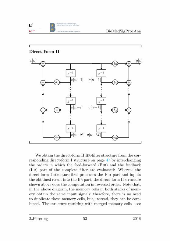
Direct Form II

z−1

v[n−N ]aN

z−1

v[n−l]al+

z−1

v[n−1]a1+

+x[n]

z−1

v[n−M ]bM

z−1

v[n−k]bk +

z−1

v[n−1]b1 +

b0 +y[n]

We obtain the direct-form II Iir-filter structure from the cor-responding direct-form I structure on page 47 by interchangingthe orders in which the feed-forward (Fir) and the feedback(Iir) part of the complete filter are evaluated: Whereas thedirect-form I structure first processes the Fir part and inputsthe obtained result into the Iir part, the direct-form II structureshown above does the computation in reversed order. Note that,in the above diagram, the memory cells in both stacks of mem-ory obtain the same input signals; therefore, there is no needto duplicate these memory cells, but, instead, they can be com-bined. The structure resulting with merged memory cells—see

3 Filtering 53 2018

BioMedSigProcAna

the next diagram—is usually called the direct-form II Iir-filterstructure. The direct-form II structure is sometimes also called“poles first” structure.

Direct Form II with Merged Memories

z−1

v[n−N ]�a

N

z−1

v[n−k]�ak+

z−1

v[n−1]�

a1+

+x[n]

z−1

bN

z−1

bk +

z−1

b1 +

b0 + y[n]

We have defined in the above diagram the parameter N asthe maximum between the transfer function’s numerator degreeM and its denominator degree N ; that is, N is the amount ofmemory cells minimally needed. Obviously, we have for M < Nthe corresponding coefficients bi being zero, and for N < M thecorresponding coefficients al being zero.

The Signal Processing Toolbox and the Dsp System Toolboxof Matlab use dfilt.df2() to construct a direct-form II Iir-filter object.

3 Filtering 54 2018

BioMedSigProcAna

Direct Form II Sos: Cascade of Sos’s


z−1

v[n−2]�a2

z−1

v[n−1]�a1+

+x[n]

z−1

b2

z−1

b1 +

b0 +y[n]

3 Filtering 55 2018

BioMedSigProcAna

Direct Form II Sos: Cascade of Sos’s (cont’d)

• the cascade of direct form II second-order sections

x[n]g0

DfII

Sos1 g1

DfII

Sos2 g2

DfII

Sosm gm

y[n]

The Signal Processing Toolbox and the Dsp System Toolboxof Matlab use dfilt.df2sos() to construct a direct-form IIsecond-order sections filter object.

Here again, the values gi in the above diagram are the gainsfor each section, see page 49.


3 Filtering 56 2018

BioMedSigProcAna

Transposed Direct Form II

z−1

bN +

z−1

bk +

z−1

b1 +

b0 +x[n]

z−1

aN

vN [n])

z−1

ak+

vk[n])

z−1

a1+

v1[n])

+ y[n]

We have again defined in the above diagram the parameterN as the maximum between the transfer function’s numera-tor degree M and its denominator degree N ; that is, N is theamount of memory cells minimally needed. Obviously, we havefor M < N the corresponding coefficients bi being zero, and forN < M the corresponding coefficients al being zero.

The Signal Processing Toolbox and the Dsp System Toolboxof Matlab use dfilt.df2t() to construct a transposed direct-form II Iir-filter object.

3 Filtering 57 2018

BioMedSigProcAna

The Matlab function filter() implements in its defaultfunction call17 the transposed direct-form II Iir-filter structureshown on page 57. Using the state variables vk[n] introduced inthat diagram, the filter() function computes at sample-timen the difference equation as follows:

y[n] = b0 x[n] + v1[n − 1] ,

v1[n] = b1 x[n] + v2[n − 1] + a1 y[n] ,

... =...

...

vN−1[n] = bN−1 x[n] + vN [n − 1] + aN−1 y[n] ,

vN [n] = bN x[n] + aN y[n] .

17In the most simple situation, a discrete-time filter is defined by thenumerator and denominator polynomials of its z-transformation transfer-function H(z) = N(z)/D(z), and these polynomials are specified in Mat-

lab as the vectors of their coefficients, say, num and den, respectively. If thecommand filter() is then used as yy = filter(num,den,xx) with xx thevector containing the input signal, then Matlab computes the transposeddirect-form II, as indicated. However, if we apply the command filter()

to a previously defined filter object, which contains information about thedesired structure, then Matlab computes, of course, according to the spec-ified structure.

3 Filtering 58 2018

BioMedSigProcAna

Transposed Direct Form II Sos: Cascade of Sos’s


z−1

b2 +

z−1

b1 +

b0 +input

z−1

a2

z−1

a1+

+output

3 Filtering 59 2018

BioMedSigProcAna

Transposed Direct Form II Sos: Cascade of Sos’s (cont’d)

• the cascade of transposed direct-form II second-order sec-tions

x[n]g0

DfIIt

Sos1 g1

DfIIt

Sos2 g2

DfIIt

Sosm gm

y[n]

The Signal Processing Toolbox and the Dsp System Tool-box of Matlab use dfilt.df2tsos() to construct a transposeddirect-form II second-order sections filter object.

Here again, the values gi in the above diagram are the gainsfor each section, see page 49.


Beside the shown Iir-filter structures there exist many more.The toolboxes of Matlab know the most important of themsuch as Iir filters based on the lattice structure, but also state-space filters and filters obtained by serial (cascade) and parallelcombinations of already defined filter objects; see the relevantmanuals. You might also want to consult [Mit98, Chapter 6].

3 Filtering 60 2018

BioMedSigProcAna

5.3 Special Iir Filters

A Notch Filter

• notch filter as a generalization of a Fir nulling filter

• “imagine” the magnitude responses from the pole-zero maps

1

j

.....

.....

.....

.....

.....

..................................................................

....................

...............................................................................................................................................................................................................................................................................................................................................................................

........................................................................................................

c

c

×...............................................................................................................

...............................................................................................................

ω0

−ω02

nulling Fir

1

j

.....

.....

.....

.....

.....

..................................................................

....................

.......................................................................................................................................................................................................................................................................................................................................................................................................................................................................................

c

c

×

×

...............................................................................................................

...............................................................................................................

ω0

−ω0

.......................

.......................

.......................................................................................... .................................................................................

.........

ρ

notch Iir

Denote the poles in the pole-zero map of the “notch Iir” inthe above figure as p1,2 = ρe±jω0 , and the zeros as z1,2 = e±jω0 .Then a corresponding notch Iir-filter transfer function is18

H(z) =

(1 − z1z

−1) (

1 − z∗1z−1)

(1 − p1z−1) (1 − p∗1z−1)

=1 − 2 cos(ω0)z

−1 + z−2

1−2ρ cos(ω0)z−1+ρ2z−2.

(3)Intuitively it is clear that the closer ρ approaches unity—for

stability ρ must obviously always be strictly smaller than unity,

18Recall that the poles and the zeros of a filter do specify the filter onlyup to a constant gain; here we use as gain-constant the value one.

3 Filtering 61 2018

BioMedSigProcAna

ρ < 1—the tighter the notch becomes. The figure on the nextslide confirms this intuition.

Notch Filter: Frequency Magnitude-Responses

• the closer ρ to unity ; the tighter the notch

−π −ω0 ω0 π

1

............................................................................................................................................................................................................................................................................................................................................................................................................................................................................................................................................................................................................................................................................................................................................................................................................................................................................................................................................................................................................................................................................................................................................................................................................................................................

..............

..............

..............

..............

...............

..............

..............

..............

..............

...............

..............

..............

...............

..............

............................................................................................................................................

...............................................................................................................................................................................................................................................................................................................................................................................................................................................................................................................................................................................................................................................................................................................................................................................................................................................................................................................................................................................................................................................................................................................................................................................................................................................................................................................

..............

..............

..............

..............

..............

..............

..............

..............

...............

..............

..............

..............

..............

...............

..............

..............

..................................................................................................................................................................................................................................................................................................................................................................................................................................................................................................................................................................................................................................................................................

..............

..............

..............

..............

..............

..............

..............

..............

...............

..............

..............

..............

..............

...............

..............

..............

..................................................................................................................................................................................................................................................................................................................................................................................................................................................................................................................................................................................................................................................................................................................................................................................................................................

....................................................................................

ρ = 0.99

....................................................................................................................................................................

ρ = 0.9

The above figure shows the magnitude responses for twonotch-filter designs for notching frequency ω0 = π/5 using ρ =0.9 and ρ = 0.99, respectively. Note that the filters are, accord-ing to the transfer functions in (3), not normalized, that is, theyhave, for example, not a Dc gain that is unity.

Although we have not shown, it is intuitively clear, and youmight want to verify it, that a narrow-notch filter causes strongphase shifts in the vicinity of the notch frequency ω0.

The introduced notch filters may be generalized in severalways. We might use instead of zeros on the unit circle otherzeros, but still in the same angular directions as the poles:

z1 = ρzejω0 = z∗2 , p1 = ρpe

jω0 = p∗2 .

3 Filtering 62 2018

BioMedSigProcAna

With such a pole-zero constellation we may realize a kind ofa parametric equalizer: For ρp < ρz , ρp < 1, we still have anattenuation in the vicinity of the frequency ω0, but this atten-uation is weaker than that for the true notch with ρz = 1, andwith ρz < ρp < 1 we may also realize a boost (amplification)around ω0.

We may also generalize the introduced notch filter in thatwe not only use two, complex-conjugate, pole-zero pairs butadditional ones to construct a notch filter with notches at anarbitrary (finite) set of frequencies. We obtain then the so-calledcomb filters, compare, for example, [Orf96, Section 6.4.3, pp. 253ff.]. Such filters might be useful if a system is plagued by apower-line interference of a certain frequency and its harmonics.

If you happen to hold [Orf96] in your hands, we propose thatyou look up a few additional pages: On pages 365 ff. you findnotch-filter applications in generating digital audio effects; onpages 406 ff. you see the application of notch filters in removingpower-line interferences from Ecg signals; and on pages 583ff. you are introduced to notch-filter design techniques that arealternatives to the just discussed pole-zero placement technique,which is useful to design narrow notches but becomes tedious fornotch filters with wider peaks.

3 Filtering 63 2018

BioMedSigProcAna

5.4 Design Methods

General Iir-Filter Design Methods

oldest:

• analog prototyping

more enhanced techniques:

• direct design

• generalized Butterworth design

• parametric modeling

The analog prototyping design method uses the transfer func-tion (poles and zeros) of a classical lowpass prototype filter inthe continuous-time domain (analog filter, with correspondingLaplace-domain description), to obtain the desired discrete-timefilter through frequency transformation and filter discretization.

The direct design methods design discrete-time filters di-rectly in the discrete time-domain by approximating a piecewiselinear magnitude response.

The generalized Butterworth design method designs lowpassButterworth discrete-time filters that have more zeros than poles.

The parametric modeling design technique finds a discrete-time filter that approximates a prescribed time or frequencydomain response. This design method is closely related to thetopic of system identification.

3 Filtering 64 2018

BioMedSigProcAna

A standard reference for digital filter design techniques is[PB87]; [OS75, Section 5.3, pp. 230-237] has a nice (and short)discussion on computer-aided design methods; you might alsolike to consult the User’s Guide of Matlab’s Signal ProcessingToolbox.

Iir-Filter Design: Analog Prototyping

• uses the poles & zeros of classical, normalized, lowpassprototype-filters in continuous-time (analog filters)

• obtains from the analog prototype the desired discrete-time filter by frequency transformations & discretizations

• why a useful method?

– art of analog filter-design is highly advanced

– many analog design methods have simple close-formdesign formulae

– often, the discrete-time filter emulates an analog filter

We give a design example in [Goe18b].

The Signal Processing Toolbox of Matlab has the followingcommand-line commands—which are integrated into Gui’s suchas the sptool or the fdatool:

complete-filter design functions: besself(), butter(),ellip(), cheby1(), cheby2(), to design Bessel-, Butter-worth-, Elliptic-, and Chebyshev filters of type 1 and 2.Elliptic filters are also known as Cauer filters; Chebyshevtype 1 filters have a magnitude-response ripple in the pass-band but no ripple in the stopband, whereas Chebyshev

3 Filtering 65 2018

BioMedSigProcAna

type 2 filters have a reversed characteristic—a ripple inthe stopband but none in the passband.

filter order estimators: butterord(), cheby1ord(),cheby2ord(), ellipord().

analog lowpass filter prototypes: besselap(), buttap(),cheb1ap(), cheb2ap(), ellipap().

analog frequency transformations: the commands lp2lp(),lp2hp(), lp2bp(), and lp2bs() compute lowpass-to-low-pass, lowpass-to-highpass, lowpass-to-bandpass, and low-pass-to-bandstop transformations.

transformations to discrete time: to obtain a discrete-timesystem out of a continuous-time system, the two functionsbilinear() and impinvar() compute the bilinear- andthe impulse-invariance transformation, respectively. Notethat the Control System Toolbox gives commands for ad-ditional alternative discretization methods.

3 Filtering 66 2018

BioMedSigProcAna

Iir-Filter Design: Direct Design

• filter specification by desired frequency-response of thediscrete-time filter

• where the frequency-response specifications is a piecewise-linear magnitude response

• the method designs a discrete-time filter of supplied or-der N using a least-squares fit to the desired frequencymagnitude-response

• Matlab function: yulewalk()

3 Filtering 67 2018

BioMedSigProcAna

Iir-Filter Design: Generalized Butterworth

• analog Butterworth filters: filters having a maximally flatmagnitude response

• generalized Butterworth filters: discrete-time Butterworthfilters with differing numbers of zeros and poles

• is desirable in some implementations where poles are moreexpensive computationally than zeros

• Matlab function: maxflat()

The Matlab function maxflat() works similar as the func-tion butter(), except that one can specify two orders (one forthe numerator polynomial and one for the denominator polyno-mial of the transfer function) instead of just one. The resultingfilters are maximally flat, that is, the resulting filter is optimalfor any numerator and denominator orders, with the maximumnumber of derivatives at ω = 0 and at the Nyquist frequencyω = π both set to 0.

3 Filtering 68 2018

BioMedSigProcAna

Iir-Filter Design: Parametric Modeling

• given: a model for the filter; for example an Ar model:

y[n] = a1y[n − 1] + a2y[n − 2] + · · · + aky[n − k] + x[n]

• given: data, for example a desired impulse-response

• find: parameters of the model

– in example: a =(a1 a2 . . . ak

)T

• by minimizing error between given data and model

– in example: a = function (data, k) , k = model order

• Matlab Signal Processing Toolbox functions:

– time domain: arburg(), arcov(), armcov(), aryule(),lpc(), levinson(), prony(), stmcb()

– frequency domain: invfreqz(), invfreqs()

The acronym Ar used in the above slide stands for auto-regressive.

The parametric modeling functions operate with rationaltransfer function models. They must be given appropriate infor-mation about the desired system (impulse or frequency responsedata, or input and output sequences); they find then the coeffi-cients of a linear system that models the desired system.

One important application of the parametric modeling func-tions is in the design of filters that have a prescribed time or

3 Filtering 69 2018

BioMedSigProcAna

frequency response. The parametric modeling functions thenprovide a data-oriented alternative to the usual Iir-filter—andlikewise the Fir-filter—filter-design approaches.

We note in passing that the System Identification Toolboxof Matlab contains an even more extensive collection of para-metric modeling tools.

As an introduction to the filter design by parametric model-ing approaches you might want to read [Jac96, Chapter 10].

3 Filtering 70 2018

BioMedSigProcAna

6 Steps in Digital-Filter Designs

Overview

1. design specifications

• frequency domain: magnitude-, phase response

• time domain: impulse-, step response, . . .

2. approximation of desired characteristics

3. realization

4. implementation

note: the above four steps are not independent

If the design specifications are given in the time domain, theimpulse- and step response might be specified by notions suchas rise time, peak overshoot, and the like. More generally, wemight want to specify our filter by responses to an arbitrarywaveform.

The approximation problem is to find a causal, linear, time-invariant system via the transfer function or the impulse re-sponse.

The realization problem addresses the selection of a structurethat fulfills the design specifications even under finite-wordlengtheffects of filter coefficients and signals.

3 Filtering 71 2018

BioMedSigProcAna

The implementation problem is the construction of the filterin discrete hardware, in Vhdl description (for integrated-circuitimplementations), or in software (on a floating-point or on afixed-point digital processor).

Design Specifications: Ideal Magnitude-Responses

−π −ωc2 −ωc1 ωc1 ωc2 π

1.....................................................................................................................................................................................................

..............

..............

..............

..............

.....................................................................................................................................................................................................................................................................................................................................................................................................................

band-stop

−π −ωc2 −ωc1 ωc1 ωc2 π

1

...............................................................................................................................................................................................................................................................................................................................................................................................................

..............

..............

..............

..............

............................................................................................................................................................................................................band-pass

−π −ωc ωc π

1...................................................................................................................................................................................................................................................................................................................................................................................................................................................................................................................................

high-pass

−π −ωc ωc π

1

...................................................................................................................................................................................................................................................................................................................................................................................................................................................................................................................................

low-pass

Note that the ideal magnitude-response specifications shownabove cannot be realized due to the sharp cut-off edges. There-fore, we need what is called design templates.

3 Filtering 72 2018

BioMedSigProcAna

Design Specifications: Reality ; Design Templates

ωp ωs π

1............................................................................................................................................................................................................................................................................................................................................................

.

.

.

.

.

.

.

.

.

.

.

.

.

.

.

.

.

.

.

.

.

.

.

.

.

.

.

.

.

.

.

.

.

.

.

.

.

.

.

.

.

.

.

.

.

.

.

.

.

.

.

.

.

.

.

.

.

.

.

.

.

.

.

.

.

.

.

.

.

.

.

.

.

.

.

.

.

.

.

.

.

.

.

.

.

.

.

.

.

.

.

.

.

.

.

.

.

.

.

.

.

.

.

.

.

.

.

.

.

.

.

.

.

.

.

.

.

.

.

.

.

.

.

.

.

.

.

.

.

.

.

.

.

.

.

.

.

.

.

.

.

.

.

.

.

.

.

.

.

.

.

.

.

.

.

.

.

.

.

.

.

.

.

.

.

.

.

.

.

.

.

.

.

.

.

.

.

.

.

.

.

.

.

.

.

.

.

.

.

.

.

.

.

.

.

.

.

.

.

.

.

.

.

.

.

.

.

.

.

.

.

.

.

.

.

.

.

.

.

.

.

.

.

.

.

.

.

.

.

.

.

.

.

.

.

.

.

.

.

.

.

.

.

.

.

.

.

.

.

.

.

.

.

.

.

.

.

.

.

.

.

.

.

.

.

.

.

.

.

.

.

.

.

.

.

.

.

.

.

.

.

.

.

.

.

.

.

.

.

.

.

.

.

.

.

.

.

.

.

.

.

.

.

.

.

.

.

.

.

.

.

.

.

.

.

.

.

.

.

.

.

.

.

.

.

.

.

.

.

.

.

.

.

.

.

.

.

.

.

.

.

.

.

.

.

.

.

.

.

.

.

.

.

.

.

.

.

.

.

.

.

.

.

.

.

.

.

.

.

.

.

.

.

.

.

.

.

.

.

.

.

.

.

.

.

.

.

.

.

.

.

.

.

.

.

.

.

.

.

.

.

.

.

.

.

.

.

.

.

.

.

.

.

.

.

.

.

.

.

.

.

.

.

.

.

.

.

.

.

.

.

.

.

.

.

.

.

.

.

.

.

.

.

.

.

.

.

.

.

.

.

.

.

.

.

.

.

.

.

.

.

.

.

.

.

.

.

.

.

.

.

.

.

.

.

.

.

.

.

.

.

.

.

.

.

.

.

.

.

.

.

.

.

.

.

.

.

.

.

.

.

.

.

.

.

.

.

.

.

.

.

.

.

.

.

.

.

.

.

.

.

.

.

.

.

.

.

.

.

.

.

.

.

.

.

.

.

.

.

.

.

.

.

.

.

.

.

.

.

.

.

.

.

.

.

.

.

.

.

.

.

.

.

.

.

.

.

.

.

.

.

.

.

.

.

.

.

.

.

.

.

.

.

.

.

.

.

.

.

.

.

.

.

.

.

.

.

.

.

.

.

.

.

.

.

.

.

.

.

.

.

.

.

.

.

.

.

.

.

.

.

.

.

.

.

.

.

.

.

.

.

.

.

.

.

.

.

.

.

.

.

.

.

.

.

.

.

.

.

.

.

.

.

.

.

.

.

.

.

.

.

.

.

.

.

.

.

.

.

.

.

.

.

.

.

.

.

.

.

.

.

.

.

.

.

.

.

.

.

.

.

.

.

.

.

.

.

.

.

.

.

.

.

.

.

.

.

.

.

.

.

.

.

.

.

.

.

.

.

.

.

.

.

.

.

.

.

.

.

.

.

.

.

.

.

.

.

.

.

.

.

.

.

.

.

.

.

.

.

.

.

.

.

.

.

.

.

.

.

.

.

.

.

.

.

.

.

.

.

.

.

.

.

.

.

.

.

.

.

.

.

.

.

.

.

.

.

.

.

.

.

.

.

.

.

.

.

.

.

.

.

.

.

.

.

.

.

.

.

.

.

.

.

.

.

.

.

.

.

.

.

.

.

.

.

.

.

.

.

.

.

.

.

.

.

.

.

.

.

.

.

.

.

.

.

.

.

.

.

.

.

.

.

.

.

.

.

.

.

.

.

.

.

.

.

.

.

.

.

.

.

.

.

.

.

.

.

.

.

.

.

.

.

.

.

.

.

.

.

.

.

.

.

.

.

.

.

.

.

.

.

.

.

.

.

.

.

.

.

.

.

.

.

.

.

.

.

.

.

.

.

.

.

.

.

.

.

.

.

.

.

.

.

.

.

.

.

.

.

.

.

.

.

.

.

.

.

.

.

.

.

.

.

.

.

.

.

.

.

.

.

.

.

.

.

.

.

.

.

.

.

.

.

.

.

.

.

.

.

.

.

.

.

.

.

.

.

.

.

.

.

.

.

.

.

.

.

.

.

.

.

.

.

.

.

.

.

.

.

.

.

.

.

.

.

.

.

.

.

.

.

.

.

.

.

.

.

.

.

.

.

.

.

.

.

.

.

.

.

.

.

.

.

.

.

.

.

.

.

.

.

.

.

.

.

.

.

.

.

.

.

.

.

.

.

.

.

.

.

.

.

.

.

.

.

.

.

.

.

.

.

.

.

.

.

.

.

.

.

.

.

.

.

.

.

.

.

.

.

.

.

.

.

.

.

.

.

.

.

.

.

.

.

.

.

.

.

.

.

.

.

.

.

.

.

.

.

.

.

.

.

.

.

.

.

.

.

.

.

.

.

.

.

.

.

.

.

.

.

.

.

.

.

.

.

.

.

.

.

.

.

.

.

.

.

.

.

.

.

.

.

.

.

.

.

.

.

.

.

.

.

.

.

.

.

.

.

.

.

.

.

.

.

.

.

.

.

.

.

.

.

.

.

.

.

.

.

.

.

.

.

.

.

.

.

.

.

.

.

.

.

.

.

.

.

.

.

.

.

.

.

.

.

.

.

.

.

.

.

.

.

.

.

.

.

.

.

.

.

.

.

.

.

.

.

.

.

.

.

.

.

.

.

.

.

.

.

.

.

.

.

.

.

.

.

.....................................................................................................................................................................................................

.

.

.

.

.

.

.

.

.

.

.

.

.

.

.

.

.

.

.

.

.

.

.

.

.

.

.

.

.

.

.

.

.

.

.

.

.

.

.

.

.

.

.

.

.

.

.

.

.

.

.

.

.

.

.

.

.

.

.

.

.

.

.

.

.

.

.

.

.

.

.

.

.

.

.

.

.

.

.

.

.

.

.

.

.

.

.

.

.

.

.

.

.

.

.

.

.

.

.

.

.

.

.

.

.

.

.

.

.

.

.

.

.

.

.

.

.

.

.

.

.

.

.

.

.

.

.

.

.

.

.

.

.

.

.

.

.

.

.

.

.

.

.

.

.

.

.

.

.

.

.

.

.

.

.

.

.

.

.

.

.

.

.

.

.

.

.

.

.

.

.

.

.

.

.

.

.

.

.

.

.

.

.

.

.

.

.

.

.

.

.

.

.

.

.

.

.

.

.

.

.

.

.

.

.

.

.

.

.

.

.

.

.

.

.

.

.

.

.

.

.

.

.

.

.

.

.

.

.

.

.

.

.

.

.

.

.

.

.

.

.

.

.

.

.

.

.

.

.

.

.

.

.

.

.

.

.

.

.

.

.

.

.

.

.

.

.

.

.

.

.

.

.

.

.

.

.

.

.

.

.

.

.

.

.

.

.

.

.

.

.

.

.

.

.

.

.

.

.

.

.

.

.

.

.

. .............................................................................................................................................................................................................................................................................................................................................................................................................................................................................................................................................................................................................................................................................................................

.

.

.

.

.

.

.

.

.

.

.

.

.

.

.

.

.

.

.

.

.

.

.

.

.

.

.

.

.

.

.

.

.

.

.

.

.

.

.

.

.

.

.

.

.

.

.

.

.

.

.

.

.

.

.

.

.

.

.

.

.

.

.

.

.

.

.

.

.

.

.

.

.

.

.

.

.

.

.

.

.

.

.

.

.

.

.

.

.

.

.

.

.

.

.

.

.

.

.

.

.

.

.

.

.

.

.

.

.

.

.

.

.

.

.

.

.

.

.

.

.

.

.

.

.

.

.

.

.

.

.

.

.

.

.

.

.

.

.

.

.

.

.

.

.

.

.

.

.

.

.

.

.

.

.

.

.

.

.

.

.

.

.

.

.

.

.

.

.

.

.

.

.

.

.

.

.

.

.

.

.

.

.

.

.

.

.

.

.

.

.

.

.

.

.

.

.

.

.

.

.

.

.

.

.

.

.

.

.

.

.

.

.

.

.

.

.

.

.

.

.

.

.

.

.

.

.

.

.

.

.

.

.

.

.

.

.

.

.

.

.

.

.

.

.

.

.

.

.

.

.

.

.

.

.

.

.

.

.

.

.

.

.

.

.

.

.

.

.

.

.

.

.

.

.

.

.

.

.

.

.

.

.

.

.

.

.

.

.

.

.

.

.

.

.

.

.

.

.

.

.

.

.

.

.

.

.

.

.

.

.

.

.

.

.

.

.

.

.

.

.

.

.

.

.

.

.

.

.

.

.

.

.

.

.

.

.

.

.

.

.

.

.

.

.

.

.

.

.

.

.

.

.

.

.

.

.

.

.

.

.

.

.

.

.

.

.

.

.

.

.

.

.

.

.

.

.

.

.

.

.

.

.

.

.

.

.

.

.

.

.

.

.

.

.

.

.

.

.

.

.

.

.

.

.

.

.

.

.

.

.

.

.

.

.

.

.

.

.

.

.

.

.

.

.

.

.

.

.

.

.

.

.

.

.

.

.

.

.

.

.

.

.

.

.

.

.

.

.

.

.

.

.

.

.

.

.

.

.

.

.

.

.

.

.

.

.

.

.

.

.

.

.

.

.

.

.

.

.

.

.

.

.

.

.

.

.

.

.

.

.

.

.

.

.

.

.

.

.

.

.

.

.

.

.

.

.

.

.

.

.

.

.

.

.

.

.

.

.

.

.

.

.

.

.

.

.

.

.

.

.

.

.

.

.

.

.

.

.

.

.

.

.

.

.

.

.

.

.

.

.

.

.

.

.

.

.

.

.

.

.

.

.

.

.

.

.

.

.

.

.

.

.

.

.

.

.

.

.

.

.

.

.

.

.

.

.

.

.

.

.

.

.

.

.

.

.

.

.

.

.

.

.

.

.

.

.

.

.

.

.

.

.

.

.

.

.

.

.

.

.

.

.

.

.

.

.

.

.

.

.

.

.

.

.

.

.

.

.

.

.

.

.

.

.

.

.

.

.

.

.

.

.

.

.

.

.

.

.

.

.

.

.

.

.

.

.

.

.

.

.

.

.

.

.

.

.

.

.

.

.

.

.

.

.

.

.

.

.

.

.

.

.

.

.

.

.

.

.

.

.

.

.

.

.

.

.

.

.

.

.

.

.

.

.

.

.

.

.

.

.

.

.

.

.

.

.

.

.

.

.

.

.

.

.

.

.

.

.

.

.

.

.

.

.

.

.

.

.

.

.

.

.

.

.

.

.

.

.

.

.

.

.

.

.

.

.

.

.

.

.

.

.

.

.

.

.

.

.

.

.

.

.

.

.

.

.

.

.

.

.

.

.

.

.

.

.

.

.

.

.

.

.

.

.

.

.

.

.

.

.

.

.

.

.

.

.

.

.

.

.

.

.

.

.

.

.

.

.

.

.

.

.

.

.

.

.

.

.

.

.

.

.

.

.

.

.

.

.

.

.

.

.

.

.

.

.

.

.

.

.

.

.

.

.

.

.

.

.

.

.

.

.

.

.

.

.

.

.

.

.

.

.

.

.

.

.

.

.

.

.

.

.

.

.

.

.

.

.

.

.

.

.

.

.

.

.

.

.

.

.

.

.

.

.

.

.

.

.

.

.

.

.

.

.

.

.

.

.

.

.

.

.

.

.

.

.

.

.

.

.

.

.

.

.

.

.

.

.

.

.

.

.

.

.

.

.

.

.

.

.

.

.

.

.

.

.

.

.

.

.

.

.

.

.

.

.

.

.

.

.

.

.

.

.

.

.

.

.

.

.

.

.

.

.

.

.

.

.

.

.

.

.

.

.

.

.

.

.

.

.

.

.

.

.

.

.

.

.

.

.

.

.

.

.

.

.

.

.

.

.

.

.

.

.

.

.

.

.

.

.

.

.

.

.

.

.

.

.

.

.

.

.

.

.

.

.

.

.

.

.

.

.

.

.

.

.

.

.

.

.

.

.

.

.

.

.

.

.

.

.

.

.

.

.

.

.

.

.

.

.

.

.

.

.

.

.

.

.

.

.

.

.

.

.

.

.

.

.

.

.

.

.

.

.

.

.

.

.

.

.

.

.

.

.

.

.

.

.

.

.

.

.

.

.

.

.

.

.

.

.

.

.

.

.

.

.

.

.

.

.

.

.

.

.

.

.

.

.

.

.

.

.

.

.

.

.

.

.

.

.

.

.

.

.

.

.

.

.

.

.

.

.

.

.

.

.

.

.

.

.

.

.

.

.

.

.

.

.

.

.

.

.

.

.

.

.

.

.

.

.

.

.

.

.

.

.

.

.

.

.

.

.

.

.

.

.

.

.

.

.

.

.

.

.

.

.

.

.

.

.

.

.

.

.

.

.

.

.

.

.

.

.

.

.

.

.

.

.

.

.

.

.

.

.

.

.

.

.

.

.

.

.

.

.

.

.

.

.

.

.

.

.

.

.

.

.

.

.

.

.

.

.

.

.

.

.

.

.

.

.

.

.

.

.

.

.

.

.

.

.

.

.

.

.

.

.

.

.

.

.

.

.

.

.

.

.

.

.

.

.

.

.

.

.

.

.

.

.

.

.

.

.

.

.

.

.

.

.

.

.

.

.

.

.

.

.

.

.

.

.

.

.

.

.

.

.

.

.

.

.

.

.

.

.

.

.

.

.

.

.

.

.

.

.

.

.

.

.

.

.

.

.

.

.

.

.

.

.

.

.

.

.

.

.

.

.

.

.

.

.

.

.

.

.

.

.

.

.

.

.

.

.

.

.

.

.

.

.

.

.

.

.

.

.

.

.

.

.

.

.

.

.

.

.

.

.

.

.

.

.

.

.

.

.

.

.

.

.

.

.

.

.

.

.

.

.

.

.

.

.

.

.

.

.

.

.

.

.

.

.

.

.

.

.

.

.

.

.

.

.

.

.

.

.

.

.

.

.

.

.

.

.

.

.

.

.

.

.

.

.

.

.

.

.

.

.

.

.

.

.

.

.

.

.

.

.

.

.

.

.

.

.

.

.

.

.

.

.

.

.

.

.

.

.

.

.

.

.

.

.

.

.

.

.

.

.

.

.

.

.

.

.

.

.

.

.

.

.

.

.

.

.

.

.

.

.

.

.

.

.

.

.

.

.

.

.

.

.

.

.

.

.

.

.

.

.

.

.

.

.

.

.

.

.

.

.

.

.

.

.

.

.

.

.

.

.

.

.

.

.

.

.

.

.

.

.

.

.

.

.

.

.

.

.

.

.

.

.

.

.

.

.

.

.

.

.

.

.

.

.

.

.

.

.

.

.

.

.

.

.

.

.

.

.

.

.

.

.

.

.

.

.

.

.

.

.

.

.

.

.

.

.

.

.

.

.

.

.

.

.

.

.

.

.

.

.

.

.

.

.

.

.

.

.

.

.

.

.

.

.

.

.

.

.

.

.

.

.

.

.

.

.

.

.

.

.

.

.

.

.

.

.

.

.

.

.

.

.

.

.

.

.

.

.

.

.

.

.

.

.

.

.

.

.

.

.

.

.

.

.

.

.

.

.

.

.

.

.

.

.

.

.

.

.

.

.

.

.

.

.

.

.

.

.

.

.

.

.

.

.

.

.

.

.

.

.

.

.

.

.

.

.

.

.

.

.

.

.

.

.

.

.

.

.

.

.

.

.

.

.

.

.

.

.

.

.

.

.

.

.

.

.

.

.

.

.

.

.

.

.

.

.

.

.

.

.

.

.

.

.

.

.

.

.

.

.

.

.

.

.

.

.

.

.

.

.

.

.

.

.

.

.

.

.

.

.

.

.

.

.

.

.

.

.

.

.

.

.

.

.

.

.

.

.

.

.

.

.

.

.

.

.

.

.

.

.

.

.

.

.

.

.

.

.

.

.

.

.

.

.

.

.

.

.

.

.

.

.

.

.

.

.

.

.

.

.

.

.

.

.

.

.

.

.

.

.

.

.

.

.

.

.

.

.

.

.

.

.

.

.

.

.

.

.

.

.

.

.

.

.

.

.

.

.

.

.

.

.

.

.

.

.

.

.

.

.

.

.

.

.

.

.

.

.

.

.

.

.

.

.

.

.

.

.

.

.

.

.

.

.

.

.

.

.

.

.

.

.

.

.

.

.

.

.

.

.

.

.

.

.

.

.

.

.

.

.

.

.

.

.

.

.

.

.

.

.

.

.

.

.

.

.

.

.

.

.

.

.

.

.

.

.

.

.

.

.

.

.

.

.

.

.

.

.

.

.

.

.

.

.

.

.

.

.

.

.

.

.

.

.

.

.

.

.

.

.

.

.

.

.

.

.

.

.

.

.

.

.

.

.

.

.

.

.

.

.

.

.

.

.

.

.

.

.

.

.

.

.

.

.

.

.

.

.

.

.

.

.

.

.

.

.

.

.

.

.

.

.

.

.

.

.

.

.

.

.

.

.

.

.

.

.

.

.

.

.

.

.

.

.

.

.

.

.

.

.

.

.

.

.

.

.

.

.

.

.

.

.

.

.

.

.

.

.

.

.

.

.

.

.

.

.

.

.

.

.

.

.

.

.

.

.

.

.

.

.

.

.

.

.

.

.

.

.

.

.

.

.

.

.

.

.

.

.

.

.

.

.

.

.

.

.

.

.

.

.

.

.

.

.

.

.

.

.

.

.

.

.

.

.

.

.

.

.

.

.

.

.

.

.

.

.

.

.

.

.

.

.

.

.

.

.

.

.

.

.

.

.

.

.

.

.

.

.

.

.

.

.

.

.

.

.

.

.

.

.

.

.

.

.

.

.

.

.

.

.

.

.

.

.

.

.

.

.

.

.

.

.

.

.

.

.

.

.

.

.

.

.

.

.

.

.

.

.

.

.

.

.

.

.

.

.

.

.

.

.

.

.

.

.

.

.

.

.

.

.

.

.

.

.

.

.

.

.

.

.

.

.

.

.

.

.

.

.

.

.

.

.

.

.

.

.

.

.

.

.

.

.

.

.

.

.

.

.

.

.

.

.

.

.

.

.

.

.

.

.

.

.

.

.

.

.

.

.

.

.

.

.

.

.

.

.

.

.

.

.

.

.

.

.

.

.

.

.

.

.

.

.

.

.

.

.

.

.

.

.

.

.

.

.

.

.

.

.

.

.

.

.

.

.

.

.

.

.

.

.

.

.

.

.

.

.

.

.

.

.

.

.

.

.

.

.

.

.

.

.

.

.

.

.

.

.

.

.

.

.

.

.

.

.

.

.

.

.

.

.

.

.

.

.

.

.

.

.

.

.

.

.

.

.

.

.

.

.

.

.

.

.

.

.

.

.

.

.

.

.

.

.

.

.

.

.

.

.

.

.

.

.

.

.

.

.

.

.

.

.

.

.

.

.

.

.

.

.

.

.

.

.

.

.

.

.

.

.

.

.

.

.

.

.

.

.

.

.

.

.

.

.

.

.

.

.

.

.

.

.

.

.

.

.

.

.

.

.

.

.

.

.

.

.

.

.

.

.

.

.

.

.

.

.

.

.

.

.

.

.

.

.

.

.

.

.

.

.

.

.

.

.

.

.

.

.

.

.

.

.

.

.

.

.

.

.

.

.

.

.

.

.

.

.

.

.

.

.

.

.

.

.

.

.

.

.

.

.

.

.

.

.

.

.

.

.

.

.

.

.

.

.

.

.

.

.

.

.

.

.

.

.

.

.

.

.

.

.

.

.

.

.

.

.

.

.

.

.

.

.

.

.

.

.

.

.

.

.

.

.

.

.

.

.

.

.

.

.

.

.

.

.

.

.

.

.

.

.

.

.

.

.

.

.

.

.

.

.

.

.

.

.

.

.

.

.

.

.

.

.

.

.

.

.

.

.

.

.

.

.

.

.

.

.

.

.

.

.

.

.

.

.

.

.

.

.

.

.

.

.

.

.

.

.

.

.

.

.

.

.

.

.

.

.

.

.

.

.

.

.

.

.

.

.

.

.

.

.

.

.

.

.

.

.

.

.

.

.

.

.

.........................................................................................

...............................................................................................................................................................................................................................................................................................................................................................................................................................................

.........................................................................................................................................

.....

.....

.....

...........

........

.......................

...

.....

...2δp

.....

.....

...........

........

................

...

.....

...2δs

................................................................................................. ......................................................................................... ........

passband...................................................................... .............................................................. ........

regiontransition

................................................................................................................................................................................. ................................................................................................................... ........

stopband

• ωp = passband cut-off frequency

• δp = passband ripple

• ωs = stopband cut-off frequency

• δs = stopband ripple

It is obvious from the above figure that the transition regionhas a width ∆ωt = ωs − ωp. Intuitively, it is also obvious that atighter transition region is more demanding on the filter design;likewise, smaller values of the parameters δp and δs are moredemanding on the filter design.

3 Filtering 73 2018

BioMedSigProcAna

Approximation: Iir- Versus Fir Filter

Iir filters: transfer function

H(z) =Y (z)

X(z)=

b0 + b1z−1 + · · · + bMz−M

1 − a1z−1 − · · · − aNz−N

• approximation with rational transfer function

• design parameters:

– poles

– zeros

3 Filtering 74 2018

BioMedSigProcAna

Approximation: Iir- Versus Fir Filter (cont’d)

Fir filters: transfer function

H(z) =Y (z)

X(z)= b0 + b1z

−1 + · · · + bMz−M

=b0z

M + b1zM−1 + · · · + bM

zM

• approximation with polynomial transfer function

• design parameters: zeros only

• in time domain: impulse response of length M + 1

• for approximation of a desired time-domain characteristic:a finite number of impulse-response samples are designparameters

3 Filtering 75 2018

BioMedSigProcAna

Approximation: Iir- Versus Fir Filter (cont’d)

characteristics, advantages and disadvantages:

stability: Fir are always stable, Iir might become unstable

linear phase: Fir can have exactly linear phase, Iir cannot

computational expense: high for Fir, low for Iir; to achievea given level of performance

filter functions: that can be realized

• both, Iir- and Fir-filter types: Lp, Hp, Bp, Bs

• additionally with Fir: differentiator, Hilbert-trans-former, multiband filter

• additionally with Iir: integrator, allpass filter

non-ideal effects: low for Fir, high for Iir

design methods: generally linear for Fir, non-linear for Iir

start-up transient: finite duration for Fir, dies away for Iir

The acronyms used above mean Lp = lowpass, Hp = high-pass, Bp = bandpass, and Bs = bandstop.

Concerning the computational expense of a filter realization,the order of a filter is a direct indicator of how many operationsare needed to compute one output sample. Because Fir filtersrequire a much higher filter-order than Iir filters do to achievea given level of performance, it is obvious that Fir filters arecomputationally more expense than Iir filters.

3 Filtering 76 2018

BioMedSigProcAna

Realization: Select Structure

• Fir: often direct form

• Iir: often building blocks of low order

– first-order block / second-order block (biquad)

; combined in cascade (serial) / parallel

– to produce the needed higher-order filter

– often: cascade of second-order sections (Sos)

questions

∗ which poles together with which zeros?

∗ which order of blocks in the cascade?

answers rules of thumb

advantage relative insensitivity of Sos-cascade struc-ture to coefficient quantization and round-off noise

For the above mentioned rules of thumb you might want toconsult [Jac96]; likewise, we discuss some of them in [Goe18d].To give an example, consider the Matlab function tf2sos()—convert a discrete-time filter transfer function to a second-ordersections form—which uses the following rules: First, the com-mand groups the poles and the zeros into complex conjugatepairs. Next, it matches pole and zero pairs as (i) match thepoles closest to the unit circle with the zeros closest to thosepoles; (ii) match the poles next closest to the unit circle withthe zeros closest to those poles; (iii) continue until all of thepoles and zeros are matched. It groups real poles into sectionswith the real poles closest to them in absolute value, the samerule holding for real zeros. Finally, it orders the sections in the

3 Filtering 77 2018

BioMedSigProcAna

cascade according to the proximity of the pole pairs to the unitcircle; normally it orders the sections with poles closest to theunit circle last in the cascade, but one might reverse the order.

The mentioned relative insensitivity of Sos-cascade struc-tures to coefficient quantization and round-off noise is meantas compared to direct-form structures. Such robust realizationsare especially important for Iir filters with poles very close tothe unit circle.

Realization: Determine Word-Lengths

• most important in scaling for fixed-point

• during the design phase: filter coefficients are determinedwith high precision

• in realization: finite word-lengths only

– ; for an Iir filter this might turn a stable filter intoan unstable one

– ; might violate design specifications

– ; connection to structure

• a note: proper treatment of scaling must be solved in con-nection with Sos ordering

Oppenheim and Schafer [OS89] give in Sections 6.7 through6.10 a detailed study of the word-length effects and the charac-terization of the resulting errors. You might also want to consult[OS75, Chapter 9]; also see our document [Goe18d].

3 Filtering 78 2018

BioMedSigProcAna

7 Adaptive Filters

7.1 Basics

Statistical signal processing and statistical communication the-ory most often base on assumptions like linearity of systems andGaussianity and stationarity of the stochastic processes used assignal models; the desire to obtain model-based algorithms us-ing tractable mathematics motivates these assumptions. How-ever, many of the practically encountered signals carrying infor-mation, such as biomedical signals, but also signals like music,radar, sonar, and the like, are non-stationary and non-Gaussian.An alternative to approaches that are limited by assumptions ofstationarity, Gaussianity, and linearity is to use adaptive sys-tems for signal processing: adaptive filtering does not requireknowledge of the statistics of the input data and can, therefore,be applied in situations where the above assumptions do nothold.

Practical applications of adaptive filtering are, among oth-ers, system identifications and echo cancellation. More gener-ally, adaptive systems arise in antenna systems, radar and sonarsystems, communication systems, control systems, biomedicalsystems, seismology and many more.

We note that adaptive filtering is closely related to the topicof neural networks . Adaptive filters then have to be viewed inthe broader sense of adaptive systems .

A well known reference book on adaptive filters is [Hay02].We also like [WS85], which is one of the first, but still rele-vant, textbooks on the topic. A nice and short introductionto adaptive systems is the short paper [Hay99]. You may alsowant to read Contribution 18 in the handbook [MW98], pages18.1–18.18, and also take a glimpse on Sections 19 to 23 in thathandbook. If you like to study adaptive filters that are based

3 Filtering 79 2018

BioMedSigProcAna

on Fir filters only, you may want to read [GBT99]. A recent,experimentally oriented book is [PR06].

Adaptive Systems: Ingredients

• a set of input-output pairs (input-output examples !)

di = f(xi) , i = 1, 2, . . . , N

output = function(input) , for many pairs

• a network F (·) with adjustable weights

• a comparator

• a control algorithm

In what follows, we denote vectors by boldface lowercasetypes, such as xi; vectors are always column vectors, and if weneed row vectors, we use transposed column vectors such as xT

i .Scalars are written in normal mathematical types. Finally, wedenote matrices by boldface uppercase types, such as M .

3 Filtering 80 2018

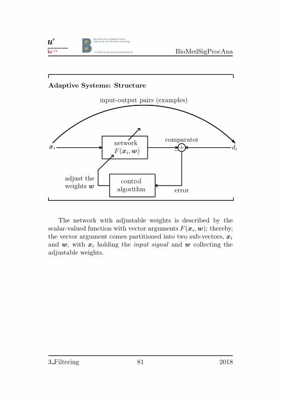
BioMedSigProcAna

Adaptive Systems: Structure

networkF (xi, w)

comparator+−

error

controlalgorithm

adjust theweights w

xi di

.........................................

..............................................

.....................................................

....................................................................

.........................................................................................................................

.............................................................................................................................................................................................................................................................................................................................................................................................................................................. ......................... ..............

input-output pairs (examples)

The network with adjustable weights is described by thescalar-valued function with vector arguments F (xi, w); thereby,the vector argument comes partitioned into two sub-vectors, xi

and w, with xi holding the input signal and w collecting theadjustable weights.

3 Filtering 81 2018

BioMedSigProcAna

Adaptive Systems: Performance Measure

• performance measure = cost function E

E = E(w) = function of weights

=1

2

N∑

i=1

(di − F (xi, w)

)2

= “total error energy”

We note that the factor 1/2 in the above concrete defini-tion of the cost function E just serves convenience: subsequentformulae become simpler.

3 Filtering 82 2018

BioMedSigProcAna

7.2 Applications

Adaptive Systems: System Identification

plant

+−e

d

y

x adaptive

filter

system

input

system

output

Mathematical modeling is fundamental in sciences and en-gineering: A model of a given system—a plant—is the mathe-matical description of the system.

In the class of applications of adaptive filters that deals withsystem identification, the adaptive filter provides a linear modelthat is the best fit—in some sense—to a given but unknownplant. The plant and the adaptive filter both obtain the sameinput, and the output of the plant plays the role of the desiredresponse for the adaptive filter. If the plant is time-invariant,the adaptive filter converges to a time-invariant linear filter; ifthe plant is time variant, the model delivered by the adaptivefilter will also be time varying.

3 Filtering 83 2018

BioMedSigProcAna

Adaptive Systems: Inverse Modeling

plantx adaptive

filter

+−

delay

e

d

y

system

input

system

output

In the class of applications of adaptive filters called inversesystem modeling, the adaptive filter provides an inverse model ofthe unknown (possibly noisy) plant that is the best fit—in somesense. In the ideal linear case the inverse model has a trans-fer function the equals the reciprocal (inverse) of the transferfunction of the plant. The desired input to the adaptive filteris normally a delayed version of plant input, but in some situa-tions, the plant input is directly used.

Note that for linear plants it is necessary that they are min-imum phase, that is, that they have all their zeros inside ofthe unit circle, to make possible the outlined straightforwardinverse system modeling. This is because the zeros of the plantto be modeled become the poles of the adaptive filter afterconvergence—the poles of the inverse system model, and thesepoles must be, of course, inside of the unit circle to yield a stableinverse system model.

Applications of inverse system modeling include, but are notrestricted to, predictive de-convolution and adaptive equaliza-tion.

3 Filtering 84 2018

BioMedSigProcAna

Adaptive Systems: Interference Cancelling

x adaptive

filter

y+−

e

d

reference

input

primary

input

system

output

In interference cancelling applications of adaptive filters, theadaptive filter suppresses an unknown signal that interferes aninformation-bearing signal at the primary input to the noisecanceler (the noise canceler is the complete system); the sup-pression is optimized in some sense. The primary input servesas the desired response for the adaptive filter, and a reference(auxiliary) input is the input to the adaptive filter. The ref-erence input signal stems from one or several sensors that arelocated in relation to the sensor that supplies the primary in-put signal in such a way that the interference, that corruptsthe information-bearing signal at the primary input, and thereference input signal are somehow correlated.

To be more concrete, let the primary input be the usefulsignal plus noise,

primary input = d[k] = s[k] + n[k] ,

where s[k] and n[k] are said useful signal and noise, respectively;and let the reference input be a noise measurement that is cor-

3 Filtering 85 2018

BioMedSigProcAna

related with the noise on the primary input:

reference input = x[k] = n[k] ,

where n[k] and n[k] denote the noise processes that are corre-lated. The correlation between the two noise processes might beexpressed by saying that one noise process is the filtered versionof the other noise process:19

n[k] = hnf [k] ∗ n[k] .

The adaptive filter in the diagram on page 85 has now the taskto model the noise filter hnf [·], that is, it tries to estimate a noiseprocess n[k] for n[k] out of the measured noise n[k]: The systemoutput in the diagram, which is the error signal for the adaptivefilter, then becomes

system output = e[k] = d[k] − y[k]

=(s[k] + n[k]

)− n[k]︸︷︷︸

≈ n[k]

≈ s[k] .

Notice then that in the present application—the interference-cancelling application—, the error signal does not converge tozero, but, instead, it actually converges to the useful input signals[k], which is contained in the primary input signal.

Applications of interference cancelling include, but are notrestricted to, adaptive noise cancelling, echo cancelling, radarpolarimetry, and adaptive beam forming.

19We here express the filtering in the time domain as the convolution ofthe input signal to the filter with its impulse response; hnf [·] is the impulseresponse of the noise filter, and ∗ denotes convolution.

3 Filtering 86 2018

BioMedSigProcAna

Adaptive Systems: Prediction

x adaptive

filter

y+−

e

d

delayinput

system

output 1

system

output 2

In prediction applications of adaptive filters, the adaptivefilter provides the best prediction—in some sense—of the presentvalue of a random signal at the system input. The present valueof the random signal thus serves as the desired response of theadaptive filter. Past values of the random signal are the input tothe adaptive filter—see the delay operator in the above diagram.Depending on the application, either the estimation (prediction)error—system output 1—, or the output of the adaptive filter—system output 2—are the output of the complete system. Ifthe system output 1 is used, the complete system works as aprediction error filter ; if the system output 2 is used, the systemworks as a predictor.

Applications of prediction include, but are not restricted to,linear predictive coding, adaptive differential pulse-code modu-lation, autoregressive spectrum analysis, and signal detection.Prediction is also an important ingredient in system identifica-tion; see, for example [Lju87], also see the System IdentificationToolbox of Matlab.

3 Filtering 87 2018

BioMedSigProcAna

7.3 Wiener Filters

Simple Fir-Filter Example: Structure

z−1 z−1x[n]

w1 w2

x[n−1] x[n−2]

+ +

w0

y[n]

⇐= xn

xn =

(x[n]x[n−1]x[n−2]

)

=

(x0n

x1n

x2n

)

• the “network” F (·, ·) is the Fir structure

• the Fir structure is a linear network

• ; determine optimum weights w0, w1, and w2

Note that at time step n the Fir filter uses the actual valuex[n] together with the stored values x[n− 1] and x[n− 2] for itscomputation. We pack these signal values used for the compu-tations at the nth time step into the signal vector xn to easethe notation in subsequent derivations.

3 Filtering 88 2018

BioMedSigProcAna

Fir-Filter Example: Computations

• the Fir filter computes

F (xn, w) = w0x[n] + w1x[n − 1] + w2x[n − 2]

=(w0 w1 w2

)

x0n

x1n

x2n

= wT xn

• the performance measure E(w) is a quadratic function ofthe weights in w

E(w) =1

2

N∑

n=1

(dn − wT xn

)2

; E(w) has a well defined minimum

Recall that our vectors are always column vectors, and thatwe use transposed column vectors—the subscript “T ” denotestranspose—if we need row vectors.

Note that the index n = 1, 2, . . . , N in the formula for theperformance measure E(w) runs over all input-output signalexamples.

3 Filtering 89 2018

BioMedSigProcAna

Fir-Filter Example: Minimum of E(w)

• for the minimum of the scalar-valued function E(w) wemust have

∂E(w)

∂wi= 0 , i = 0, 1, 2 .

• the involved derivatives are

∂E(w)

∂wi=

∂

∂wi

(1

2

N∑

n=1

(dn − F (xn, w)

)2)

=

N∑

n=1

(F (xn, w) − dn

) ∂

∂wiF (xn, w) .

In more detail we could write

∂E(w)

∂wi=

∂

∂wi

(1

2

(d1 − F (x1, w)

)2

+1

2

(d2 − F (x2, w)

)2

+ · · ·

+1

2

(dN − F (xN , w)

)2)

=(d1−F (x1, w)

)−∂F (x1, w)

∂wi+

+(d2−F (x2, w)

)−∂F (x2, w)

∂wi+ · · ·

+(dN −F (xN , w)

)−∂F (xN , w)

∂wi

=

N∑

n=1

(F (xn, w) − dn

) ∂

∂wiF (xn, w) .

3 Filtering 90 2018

BioMedSigProcAna

Fir-Filter Example: Minimum of E(w) (cont’d)

• the derivatives of the scalar-valued function F (xn, w) are

∂

∂wF (xn, w) =

∂

∂w0F (xn, w)

∂

∂w1F (xn, w)

∂

∂w2F (xn, w)

=

∂

∂w0wTxn

∂

∂w1wTxn

∂

∂w2wTxn

=

x0n

x1n

x2n

= xn

• where we recall that

wT x = w0x0n + w1x1n + w2x2n

Note that we have arranged the derivatives of the scalar func-tion F (xn, w) with respect to the weights wi in a column vector.This column vector happens to be, in the presently consideredFir case, just the input-signal vector xn. To see that this istrue, consider just the first component:

∂

∂w0wTxn =

∂

∂w0

(w0x0n + w1x1n + w2x2n

)= x0n .

3 Filtering 91 2018

BioMedSigProcAna


• ; the gradient of the scalar-valued function E(w) is

g = g(w) =

∂

∂w0E(w)

∂

∂w1E(w)

∂

∂w2E(w)

=N∑

n=1

(wT xn − dn

)xn

The gradient just arranges the derivatives of E(w) with re-spect to the individual components wi of w into a column vec-tor. In more detail we could write (recall that we have in thepresently considered Fir case F (xn, w) = wT xn)

∂

∂w0E(w)

∂

∂w1E(w)

∂

∂w2E(w)

=

N∑

n=1

(F (xn, w) − dn

)x0n

N∑

n=1

(F (xn, w) − dn

)x1n

N∑

n=1

(F (xn, w) − dn

)x2n

,

=

N∑

n=1

(wT xn − dn

)

x0n

x1n

x2n

,

=

N∑

n=1

(wT xn − dn

)xn .

3 Filtering 92 2018

BioMedSigProcAna


• denote the weight vector w that attains the minimum ofE(w) by w

• then we have for the gradient g(w) at w

g(w) = 0 ;

N∑

n=1

(w

Txn − dn

)xn = 0

• thus, the minimum-attaining weight vector becomes

w =

(N∑

n=1

xnxTn

)−1( N∑

n=1

dnxn

)

• this is the inverse of the correlation matrix of data timesthe cross-correlation between data and desired response

Starting from∑

n

(w

Txn − dn

)xn = 0 we have, in more de-

tail, the derivation steps given on the next page. Note that weindicate in these derivations, in the graphical parts accompany-ing the formulae, by bars the form of row and column vectors,such as for a row vector, and we indicate a scalar by a bullet,such as .

3 Filtering 93 2018

BioMedSigProcAna

The formula∑

n

(w

Txn − dn

)xn = 0 also reads

∑n dnxn =∑

n wTxnxn, which can be re-written as

;

∑

n

dnxn =∑

n

(w

Txn

)

︸︷︷︸× =

xn ,

=∑

n

xn

(w

Txn

),

︸︷︷︸=

=∑

n

xn

︸︷︷︸

(xT

n w)

︸︷︷︸×

=(∑

n

xnxTn

)w .

Therefore, we finally have

w =(∑

n

xnxTn

︸︷︷︸×︸︷︷︸

)−1(∑

n

dnxn

).

3 Filtering 94 2018

BioMedSigProcAna

Fir-Filter Example: Least-squares Solution

• define the sample correlation matrix of the input, and thesample cross-correlation vector between the input and thedesired response as

Rx =1

N

N∑

n=1

xnxTn , rxd =

1

N

N∑

n=1

dnxn

• then the minimum-attaining weight vector can be written

w = R−1

x rxd

• above formula is based on a single snapshot of input data

– is least squares estimation algorithm

– complexity is p3 if p = # of weights in w

– complexity is p2 with recursive least-squares solution

The above slide states that the recursive least-squares so-lution is more efficient than the standard least-squares solu-tion. This is because the recursive algorithm does not restart foreach newly arriving input-data sample the computations fromscratch, but, instead, it merely adapts the already computedresult taking into account the newly available information.

3 Filtering 95 2018

BioMedSigProcAna

Fir-Filter Example: Wiener Filter

• in the least-squares solution we have

w = w(N) , where N = sample size

• now we have

if: ergodic processes

then: the optimum weight vector wopt = wopt is

wopt = limN→∞

w(N)

= Wiener filter

= optimum linear filter

= a reference solution

Informally stated, we have that random processes are er-godic, if their time averages equal their ensemble averages. Inthe above statement we must have that the input as well asthe desired response are jointly ergodic. In that case, the sam-ple correlation matrix Rx and and the sample cross-correlationvector rxd approach, with N → ∞, constant values, say Rx andrxd. We then have the estimated weight vector w approachinga constant value as well, wopt = limN→∞ w(N) = R

−1x rxd.

3 Filtering 96 2018

BioMedSigProcAna

7.4 Least-mean Squares (Lms) Algorithm

Lms Algorithm: Basic Idea

• we have seen

– Ls algorithm: complexity p3

– Rls algorithm: complexity p2

– where p = number of weights in w

• new idea

1. use method of steepest descent; thereby, recursivelycompute needed gradient vector as a function of theweight vector w

2. simplify computation by using an instantaneous esti-mate of the needed gradient vector:

g[n] = −e[n] x[n]

where e[n] is the estimation error at time instant n

Note that the notion “new idea” above is indeed the combi-nation of two ideas: First, to compute a minimum of a functionone might use the method of steepest descent; in the consid-ered situation the function to be minimized is the quadraticcost function, which has a well-defined minimum. Furthermore,the steepest descent method computes the weight vector w in

3 Filtering 97 2018

BioMedSigProcAna

a recursive fashion. Second, the steepest descent method mustcompute at each step the gradient vector of the considered func-tion; to simplify that computation, the Lms algorithm does notuse the true gradient vector but, instead, only an instantaneousestimate of it. So the algorithm might, at certain steps, notdescend; but in the long run—in a mean sense—it will descend.

3 Filtering 98 2018

BioMedSigProcAna

Lms Algorithm: Structure

z−1 z−1x[n]

w1 w2

x[n−1] x[n−2]

+ +

w0

+−d[n]

⇐= x[n]

Lms control algorithm

w[n + 1] = w[n] + µ e[n] x[n]

e[n]

x[n]

• the signal state-vector x[n] = (x[n], x[n − 1], x[n − 2])T

• the error e[n] = d[n] − wT [n]x[n] = desired − obtained

In the above least-mean squares (Lms) weight-update algo-rithm, the weight vector is usually initialized to zero, w[n] = 0.As a computer algorithm it might be written as

set w[0] = 0 ;

compute for n = 0, 1, 2, . . .

e[n] = d[n] − wT [n] x[n] ,

w[n + 1] = w[n] + µ e[n] x[n] .

The parameter µ in the update formula for the weight vector iscalled the step-size control parameter.

3 Filtering 99 2018

BioMedSigProcAna

The Lms algorithm is very simple. It is also robust in thesense that small uncertainties and small disturbances (small dis-turbance energy) result in only small estimation errors. Thesetwo reasons—simplicity and robustness—may explain its popu-larity.

It is only fair, however, to admit that the convergence (sta-bility) analysis of the Lms algorithm is not simple. As a rule ofthumb we have that small step sizes µ tend to make the algo-rithm “more stable,” but this advantage comes at the price of aslower learning (slower convergence).

We note that the Lms adaptive-filter is a nonlinear stochasticfeedback system; the nonlinearity arises because the feedbackloop depends on the tap-input vector x[n], and the randomnessarises because of the propagation of the randomness of the inputdata and desired response into the tap-weight vector w[n]. Thiscombined presence of nonlinearity and randomness is the reasonfor the difficulties in any stability analysis. In any case, the step-size parameter µ plays the critical role, and we have to choosethe µ such that the following two forms of convergence result:

1. Convergence in the mean: The expectation of the (ran-dom) tap-weight vector approaches the (optimum) Wienersolution as the number of iterations approaches infinity.

2. Convergence in the mean square: The final (steady-state)value of the mean-square error is finite.

Although we do not discuss stability and convergence in moredetail, we have the following pragmatic hints: First, you shouldperform experiments and you should start your experimentswith a “small” value of the step-size parameter µ such thatyour filter does not diverge; then you might increase your µ stepby step. Second, the Dsp System Toolbox of Matlab suppliesan algorithm that helps in determining the maximum step-sizeparameter that is suitable for a specific Lms adaptive filter al-

3 Filtering 100 2018

BioMedSigProcAna

gorithm;20 use maxstep() to determine the maximum step sizethat still ensures that the filter converges to a solution—for de-tails see the toolbox manuals.

The algorithm on page 99 is the standard Lms algorithm.There exists many variants of it, which use different weight-update formulae. We compile some of these variants in the nexttwo tables.

Lms Algorithm: Variants

• leaky Lms algorithm

w[n + 1] = (1 − αµ)w[n] + µ e[n] x[n] .

• sign-error Lms algorithm

w[n + 1] = w[n] + µ sgn(e[n]) x[n] .

• sign-data Lms algorithm

w[n + 1] = w[n] + µ e[n] sgn(x[n]) .

• sign-sign Lms algorithm

w[n + 1] = w[n] + µ sgn(e[n]) sgn(x[n]) .

The term (1 − αµ) in the leaky Lms algorithm is called theleakage. It is introduced to further stabilize the Lms algorithm;

20There are variants of the Lms algorithm introduced above; see ourdiscussion on pages 101 and 102.


BioMedSigProcAna

it is mainly used in digital implementations. The parameter αshould satisfy 0 ≤ α < 1/µ.

The function sgn(·) appearing in the sign algorithms is de-fined to return a value 1 if the argument is strictly positive, avalue 0 if the argument is zero, and a value -1 if the argumentis strictly negative. If applied to a vector, sgn(·) works on anelement-by-element basis.

Lms Algorithm: Variants (cont’d)

• normalized Lms algorithm

w[n + 1] = w[n] +µ

ε + xT [n]x[n]e[n] x[n] .

• sign-error normalized Lms algorithm

w[n + 1] = w[n] +µ

ε + xT [n]x[n]sgn(e[n]) x[n] .

Lms algorithms having a time-varying step-size parameterare conceivable:

w[n + 1] = w[n] + µ[n] e[n] x[n] .

Because it is known that stability, convergence, and steady-statebehavior of the Lms algorithm are influenced by the filter lengthas well as the power of the input signal, a reasonable choice fora time-varying step size µ[n] is

µ[n] =const

xT [n]x[n], (4)


BioMedSigProcAna

since such a choice takes filter length and signal power into ac-count. If one additionally introduces a constant ε in the denom-inator of the time-varying step-size computation according to(4) to prevent divisions by zero, the normalized Lms algorithmshown above results.

Beside the mentioned Lms-algorithm variants there are manymore. Presently, the Dsp System Toolbox of Matlab addition-ally knows the filtered-x, the delayed, the Fft-based, the block,and the adjoint Lms algorithm.

Beside Lms algorithms, the Dsp System Toolbox presentlyalso supplies tools to design recursive least squares (Rls) basedFir adaptive filters, to design affine projection Fir adaptive fil-ters, Fir adaptive filters designed in the frequency domain, andlattice based Fir adaptive filters—we refer to the relevant man-uals of the toolbox.


BioMedSigProcAna

Symbols and Notation

We denote scalar quantities in normal lowercase math typefaces,such as x. Vectors are denoted by lowercase bold typefaces,such as x; they are always column vectors, and if we need rowvectors, we denote them by transposed (column) vectors, suchas xT with superscript “T ” indicating transpose. Finally, wedenote matrices by uppercase bold typefaces, as X .

The table below lists (some of) the used symbols:

0 Zero vector of appropriate dimension.

ak The coefficients of the denominator polynomial of anIir filter; see page 43. Note that the ak’s are alsothe feedback gains of this recursive filter. In a blockdiagram a circle-shaped block that contains a symbolak is a gain element with gain factor ak.

a Vector of coefficients ak.

bk The filter coefficients of an Fir filter; see page 21.The coefficients of the numerator polynomial of anIir filter; see page 43. In a block diagram a circle-shaped block that contains a symbol bk is a gainelement with gain factor bk.

di The ith desired signal in the realm of adaptive filters.

d[k] Desired signal in the realm of adaptive filters.

D(z) Denominator polynomial of the transfer function H(z)of a linear discrete-time system. Note that some-times we also call this polynomial A(z), because Mat-

lab does so.


BioMedSigProcAna

e[n] Error signal in the realm of adaptive filters.

E(w) Performance measure (cost function) in the realm ofadaptive filters. It is a function of the weights in thevector w.

E{X} E{X} denotes expectation or expected value or meanof the random variable X .

f Continuous-time natural frequency in Hz.

fs Sampling frequency in samples/second.

f Discrete-time natural frequency: f = f/fs.

F (·) Network with adjustable weights in the realm of adap-tive filters.

g(w) Gradient vector of the performance function E(w)in the realm of adaptive filters.

h[n] Impulse response of a discrete-time system.

H(z) Transfer function of a linear discrete-time (Dt) sys-tem. It is the z transform of the system’s impulseresponse: H(z) •—• h[n]. If a discrete-time signalx[n] with z-transform X(z) •—• x[n] is the input tothe Dt system and the signal y[n] with z-transformY (z) •—• y[n] is its output, then the transfer func-tion becomes H(z) = Y (z)/X(z).

k An integer. Often also used for the discrete-time(Dt) time variable.

l An integer. Often also used for the discrete-time(Dt) time variable.

L An integer; often used for the length of the impulseresponse of an Fir filter.


BioMedSigProcAna

m An integer. Sometimes also used for the discrete-time (Dt) time variable.

M An integer.

n Discrete-time (Dt) time variable.

n[k] Noise signal in the realm of adaptive filters.

n[k] Estimation of noise signal in the realm of adaptivefilters.

N An integer.

N(z) Numerator polynomial of the transfer function H(z)of a linear discrete-time system. Note that some-times we also call this polynomial B(z), becauseMatlab does so.

pk The kth pole of a transfer function H(z).

rxd Sample cross-correlation vector between input signaland desired response in the realm of adaptive filters.

Rx Sample correlation matrix of input signal in the realmof adaptive filters.

s[k] Useful signal in the realm of adaptive filters.

sgn(·) The sign function: It returns a value 1 if the argu-ment is strictly positive, a value 0 if the argument iszero, and a value -1 if the argument is strictly neg-ative. If sgn(·) applied to a vector, it works on anelement-by-element basis.

sinc(·) The sin(x)/x function. Note that Matlab definesit with the command sinc() as

sinc(t) =

1, for t = 0,

sin(πt)

πt, elsewhere.


BioMedSigProcAna

T Used as superscript, it denotes transposes of vectorsand matrices. If, for example, x is a column vector,we have xT its corresponding row vector.

vk[n] Internal signals in discrete-time filters.

wk The kth weight in the realm of adaptive filters

w Weight vector of weights wk in the realm of adaptivefilters.

w Minimum-attaining weight vector in the realm ofadaptive filters.

wopt Minimum-attaining limiting weight vector for ergodicprocesses. The corresponding filter is the Wiener fil-ter, which is the optimum linear filter. The contextis adaptive filters.

WM WM is the abbreviation for WM = e−j2π/M . It is aprimitive M -th root of unity: First, WM

M ≡ 1 so thatWM itself is an M -th root of unity; and, second, thesequence W 0

M , W 1M , W 2

M , . . . visits all other M M -throots of unity, therefore, WM is called “primitive.”

x[n] A discrete-time signal, which is a sequence of sam-ples. Often the input signal into a filter (a system).

x Average of sequence x[n]; see page 15.

xi The ith input signal in the realm of adaptive filters.

xn Vector of signal samples “to the time point n” in therealm of adaptive filters. In detail we have xn =(x[n] x[n − 1] . . . x[n − L])

Tif the adaptive filter

has a memory depth of length L.

X(z) If we have a discrete-time signal x[n], X(z) •—• x[n]denotes its z-transform.


BioMedSigProcAna

y[n] A discrete-time signal, which is a sequence of sam-ples. Often the output signal from a filter (from asystem).

z Variable of the z transformation; complex-valued.

zk The kth zero of a transfer function H(z).

z−1 Delay operator. In a block diagram a block thatcontains the symbol z−1 is a unit-delay block. Notethat a unit-delay block may also be interpreted as amemory cell.

α A control parameter in the leaky Lms adaptive filteralgorithm.

δp Passband ripple.

δs Stopband ripple.

δ[n] The unit-impulse sequence, that is, the sequence de-fined as

δ[n] =

{1 , for n = 00 , elsewhere

.

ε Denotes a small constant in the normalized Lms

adaptive filter algorithm.

φ Variable to denote phase shifts.

γxy Normalized correlation between two discrete-time sig-nals x[n] and y[n]; see page 15.

η[n] A discrete-time noise signal.

µ Step-size control parameter in the Lms adaptive fil-ter algorithm.


BioMedSigProcAna

ω Continuous-time radian frequency: ω = 2πf , wheref is the natural frequency in Hz.

ω Discrete-time radian frequency: ω = ωfs = ω/Ts.

ωp Discrete radian frequency of pass-band edge of a fil-ter.

ωs Discrete radian frequency of stop-band edge of a fil-ter.

∆ωt Transition-region width between passband and stop-band: ∆ωt = ωs − ωp.

π The mathematical constant describing the ratio of acircle’s circumference to its diameter; it is approxi-mately 3.14159, ;-).

ρ Often denotes the distance of a pole (or of a zero)from the origin.

σ2 Denotes a variance.

∂ Used for partial derivatives.

H(ω) Frequency response of a linear discrete-time system;it is the system’s transfer function evaluated on theunit circle: H(ω) = H(z = ejbω)

Z The integer numbers . . . ,−2,−1,−0, 1, 2, 3, . . ..


BioMedSigProcAna

The following table compiles abbreviations and acronyms thatwe use throughout the document:

Ar Auto-regressive (process, model).

Bp Bandpass (filter).

Bs Bandstop (filter).

Cd (Audio) compact disc.

Cic Cascaded integrator-comb (filter).

Ct Continuous-time; signal processing systems in con-tinuous time t.

Dc Direct current (signal).

DfI Direct-form I.

DfIt Direct-form I transposed (the transposed direct-form I).

DfII Direct-form II.

DfIIt Direct-form II transposed (the transposed direct-form II).

Dsp Digital signal processor; digital signal processing.

Dt Discrete-time; signal processing systems in dis-crete time n.

Dtft Discrete-time Fourier transform.

Ecg Electro-cardiogram (signals).

Fir Finite impulse response (filter).

Hdl Hardware description language; denotes any com-puter or programming language for the formal de-scription of (mainly digital) electronic circuits.


BioMedSigProcAna

Hp Highpass (filter).

Iir Infinite impulse response (filter).

Ip Interpolation (filter).

Ir Impulse response.

Lms Least mean squares (algorithm).

Lp Lowpass (filter).

Ls Least squares (algorithm).

Ma Moving average (filter).

Mimo multiple-input to multiple-output (system).

Rls Recursive east squares (algorithm).

Siso Single-input to single-output (system).

Sos Second-order section.

Tf Transfer function.

Vhdl Very high speed integrated circuit hardware de-scription language.


BioMedSigProcAna

References

[Bau02] Gail D. Baura. System Theory and Practical Ap-plications of Biomedical Signals. IEEE Press, NewYork, 2002. Bfh-ti Biel/Bienne Library 57.08BAURA.

[CK90] R. E. Challis and R. I. Kitney. Biomedical sig-nal processing (in four parts): Part 1. time-domainmethods. Medical & Biological Engineering & Com-puting, 28:509–524, November 1990.

[CW99] Chao-Liang Chen and Alan N. Willson Jr. A trellissearch algorithm for the design of Fir filters withsigned-powers-of-two coefficients. IEEE Trans. Cir-cuits Syst. II, 46(1):29–39, January 1999.

[EBB05] John D. Enderle, Susan M. Blanchard, andJoseph D. Bronzino. Introduction to Biomedical En-gineering. Elsevier Academic Press, Amsterdam,second edition, 2005. Bfh-ti Biel/Bienne Library615.47 ENDER.

[GBT99] George-Othon Glentis, Kostas Berberidis, and Ser-gios Theodoridis. A unified view: Efficient leastsquares adaptive algorithms for Fir transversal fil-terig. IEEE Signal Processing Magazine, 16(4):13–41, July 1999.

[Goe17] Josef Goette. Ftal Mse: Hardware Algorithms—Selected Topics in Signal Processing. Bern Univer-sity of Applied Sciences, Lecture Notes from theHuCE-microLab at the Bfh-ti Biel/Bienne, Octo-ber 2017.


BioMedSigProcAna

[Goe18a] Josef Goette. Biomedical Signal Processing andAnalysis—An Fir Filter Example: Hanning Fil-ter. Bern University of Applied Sciences, Script atthe Bfh-ti Biel/Bienne, HuCE-microLab, Febru-ary 2018.

[Goe18b] Josef Goette. Biomedical Signal Processing andAnalysis—An Iir Filter Example: A ButterworthFilter. Bern University of Applied Sciences, Script atthe Bfh-ti Biel/Bienne, HuCE-microLab, Febru-ary 2018.

[Goe18c] Josef Goette. Biomedical Signal Processing andAnalysis—Event Detection: Qrs-Complexes in Ecg

Signals. Bern University of Applied Sciences,Script at the Bfh-ti Biel/Bienne, HuCE-microLab,February 2018.

[Goe18d] Josef Goette. Biomedical Signal Processing andAnalysis—On Fixed-Point Filter Realizations. BernUniversity of Applied Sciences, Script at the Bfh-ti

Biel/Bienne, HuCE-microLab, February 2018.

[Hay99] Simon Haykin. Lessons on adaptive systems for sig-nal processing, communications, and control. IEEESignal Processing Magazine, 16(5):39–48, September1999.

[Hay02] Simon Haykin. Adaptive Filter Theory. Prentice-Hall Inc., Englewood Cliffs, N.J., 4th edition, 2002.Bfh-ti Biel/Bienne Library 519.71 HAYKI.

[Jac96] Leland B. Jackson. Digital Filters and Signal Pro-cessing with Matlab Exercises. Kluwer AcademicPublishers, Amsterdam, fifth printing 2002, 3rd edi-tion, 1996.


BioMedSigProcAna

[Lju87] Lennart Ljung. System Identification: Theory forthe User. Information and System Sciences Series.Prentice-Hall Inc., Upper Saddle River, New Jersey,1987.

[MB07] Uwe Meyer-Baese. Digital Signal Processing withField Programmable Gate Arrays. Springer Verlag,Berlin Heidelberg New York, 3rd edition, 2007.

[MBO+98] James H. McClellan, C. Sidney Burrus, Alan V. Op-penheim, Thomas W. Parks, Ronald W. Schafer,and Hans W. Schuessler. Computer-Based Exercisesfor Signal Processing Using Matlab 5. Prentice-Hall Inc., Upper Saddle River, New Jersey, 1998.Bfh-ti Biel/Bienne Library 621.391 MCCLE.

[Mit98] Sanjit K. Mitra. Digital Signal Processing: A Com-puter Based Approach. Mc Graw Hill, New York,1998. Bfh-ti Biel/Bienne Library 621.391 MITRA.

[Mit06] Sanjit K. Mitra. Digital Signal Processing: A Com-puter Based Approach. Mc Graw Hill, New York, 3rdedition, 2006. Bfh-ti Biel/Bienne Library 621.391MITRA.

[MSY98] James H. McClellan, Ronald W. Schafer, andMark A. Yoder. Dsp First: A Multimedia Approach.Prentice-Hall Inc., 1998.

[MW98] Vijay K. Madisetti and Douglas B. Williams. TheDigital Signal Processing Handbook. Ieee Press,Crc Press Llc, Boca Raton, Florida, 1998. Bfh-ti

Biel/Bienne Library 621.391 MADIS.

[NS06] Kayvan Najarian and Robert Splinter. BiomedicalSignal and Image Processing. Crc Press Llc, BocaRaton, Florida, 2006. Bfh-ti Biel/Bienne Library57.08 NAJAR.


BioMedSigProcAna

[Orf96] Sophocles J. Orfanidis. Introduction to Signal Pro-cessing. Prentice-Hall Inc., Upper Saddle River, NewJersey, 1996. Bfh-ti Biel/Bienne Library 621.391ORFAN.

[OS75] Alan W. Oppenheim and Ronald W. Schafer. Digi-tal Signal Processing. Prentice-Hall Inc., EnglewoodCliffs, N.J., 1975.

[OS89] Alan V. Oppenheim and Ronald W. Schafer.Discrete-Time Signal Processing. Prentice-Hall Inc.,Englewood Cliffs, N.J., 1989. Bfh-ti Biel/BienneLibrary 621.391 OPPEN.

[OWN97] Alan V. Oppenheim, Alan S. Willsky, and S. HamidNawab. Signals and Systems. Prentice-Hall Inc.,Englewood Cliffs, N.J., 2nd edition, 1997.

[Pap77] Athanasios Papoulis. Signal Analysis. Mc Graw Hill,New York, 1977.

[Pap84] Athanasios Papoulis. Probabiliy, Random Variables,and Stochastic Processes. Mc Graw Hill, New York,2nd edition, 1984.

[PB87] T. W. Parks and C. S. Burrus. Digital Filter Design.John Wiley & Sons, New York, 1987. Eth Bib: 307713.

[PP02] Athanasios Papoulis and S. Unnikrishna Pillai.Probabiliy, Random Variables, and Stochastic Pro-cesses. Mc Graw Hill, New York, 4th edition, 2002.

[PR06] Alexander D. Poularikas and Zayed M. Ramadan.Adaptive Filtering Primer with Matlab. Crc

Press Llc, Boca Raton, Florida, 2006. Bfh-ti

Biel/Bienne Library 519.71 POULA.


BioMedSigProcAna

[Ran02] Rangaraj M. Rangayyan. Biomedical Signal Anal-ysis: A Case-Study Approach. IEEE Press, NewYork, 2002. Bfh-ti Biel/Bienne Library 57.08RANGA.

[RM87] Richard A. Roberts and Clifford T. Mullis. DigitalSignal Processing. Addison-Wesley Publishing Co.,Reading, Mass., 1987.

[SL05] Leif Sornmo and Pablo Laguna. Bioelectrical Sig-nal Processing in Cardiac and Neurological Applica-tions. Elsevier Academic Press, Amsterdam, 2005.Bfh-ti Biel/Bienne Library 616 SOERN.

[SLB96] I. W. Selesnick, M. Lang, and C. S. Burrus. Con-strained least square design of Fir filters withoutspecified transition bands. IEEE Trans. Signal Pro-cessing, 44(8), August 1996.

[Ste03] Samuel D. Stearns. Digital Signal Processing withExamples in Matlab. Crc Press Llc, Boca Raton,Florida, 2003. Bfh-ti Biel/Bienne Library 621.391STEAR.

[Tom93] Willis J. Tompkins. Biomedical Digital Signal Pro-cessing. Prentice-Hall Inc., Englewood Cliffs, N.J.,1993. Eth Bib: +521 458.

[WS85] Bernard Widrow and S. Stearns. Adaptive SignalProcessing. Prentice-Hall Inc., Englewood Cliffs,N.J., 1985. Eth Bib: 736 608.


filtering for removing of artifacts - bfh · biomedsigprocana 2 interferences 2.1 random noise...

Documents