FINAL PERFORMANCE REPORT

As Required by

THE ENDANGERED SPECIES PROGRAM

TEXAS

Grant No. TX E-161-R

(F13AP00690)

Endangered and Threatened Species Conservation

Distinguishing the Neches River Rose Mallow (Hibiscus dasycalyx) from its congeners using genetic

and niche modeling methods

Prepared by:

Dr. Josh Banta

Carter Smith

Executive Director

Clayton Wolf

Director, Wildlife

8 September 2017

2

INTERIM REPORT

STATE: ____Texas_______________ GRANT NUMBER: ___ TX E-161-R-1__

GRANT TITLE: Distinguishing the Neches River Rose Mallow (Hibiscus dasycalyx) from its

congeners using genetic and niche modeling methods.

REPORTING PERIOD: ____1 September 2013 to 31 Auguts 2017_

OBJECTIVE(S). To resolve the taxonomic relationships among Hibiscus dasycalyx and its congeners

(H. laevis and H. moscheutos), quantify the hybridization threat posed by H. laevis and H. moscheutos to

H. dasycalyx, and create ground-truthed, geo-referenced maps of East Texas, showing the areas of

suitable habitat for H. dasycalyx versus its congeners.

Segment Objectives:

Task #1. August 2013 – October 2013: Intensive (non-destructive) leaf sampling of H. dasycalyx and its

congeners in the field.

Task #2. October 2013 – August 2015: Phylogenetic and population genetic analysis of H. dasycalyx

and its congeners using modern molecular methods.

Task #3. October 2014 – July 2015: Creation of ecological niche models.

Task #4. July – August 2015: Refinement of the ecological niche models and analysis of niche

separation among species.

Significant Deviations:

None.

Summary Of Progress:

Please see Attachment A.

Location: Angelina, Trinity, and Neches river watersheds in Cherokee, Harrison, Houston, Trinity,

Angelina, Anderson, and Neches counties, Texas.

Cost: ___Costs were not available at time of this report, they will be available upon completion of the

Final Report and conclusion of the project.__

Prepared by: _Craig Farquhar_____________ Date: 8 September 2017

Approved by: ______________________________ Date:_____8 September 2017

C. Craig Farquhar

3

ATTACHMENT A

Distinguishing the Neches River Rose Mallow (Hibiscus dasycalyx) from its congeners using genetic and niche modeling methods

Principal Investigator

Dr. Josh Banta, Assistant Professor

Department of Biology

University of Texas at Tyler

3900 University Blvd.

Tyler, TX 75799

(903) 565-5655

jbanta@uttyler.edu

Co-PIs

John Placyk (Assistant Professor)1, Marsha Williams (Research Associate)1, Lance Williams (Associate Professor)1, and Randall Small (Associate Professor)2

1Department of Biology, University of Texas at Tyler

2Department of Ecology and Evolutionary Biology, University of Tennessee – Knoxville

JP: (903) 566-7147; jplacyk@uttyler.edu

MW: (903) 565-5883; mwilliams@uttyler.edu

LW: (903) 565-5878; lwilliams@uttyler.edu

RS: (865) 974-2371; rsmall@utk.edu

Texas Parks and Wildlife Consultant

Jason Singhurst, Botanist, Nongame and Rare Species Program

Final Report

August 31, 2017

4

Abstract The Neches River Rose Mallow (Hibiscus dasycalyx) is an endemic Texas wildflower that has been listed as threatened under the Endangered Species Act. This study focused on the taxonomy and distribution of H. dasycalyx using integrative methods that combined genetics, genomics, population genetics, and ecology. The goal was to resolve the taxonomic status of H. dasycalyx relative to its co-occurring and widespread congeners, H. laevis and H. moscheutos, and then combine this information with ecological information to model their distributions on the landscape. We used two different DNA sequencing approaches: Sanger-based sequencing of the nuclear gene GRANULE-BOUND STARCH SYNTHASE I (GBSSI) together with genome-wide restriction site-associated DNA sequencing (RAD-seq) to provide an overwhelming number (thousands) of informative loci. Our findings suggest that H. dasycalyx is a separate taxon from H. laevis and H. moscheutos, and that hybridization with H. laevis is occurring. New populations of H. dasycalyx were documented in the Neches River floodplain, on the border of Trinity and Angelina Counties (in an area known as Boggy Slough). We found that H. dasycalyx is predicted to generally be closer to the banks of waterways than its congeners, and relegated to very flat, broad, frequently-flooded areas with highly erodible alluvial deposits. The ecological niche models developed by this project are available in the form of georeferenced raster maps. They can be used to choose the best sites for H. dasycalyx reintroduction and/or habitat restoration projects. Overall, our study supports H. dasycalyx as a genetically and ecologically distinct species, and suggests that hybridization with H. laevis is a pervasive threat. We recommend mitigating this threat by removing H. laevis from sites where H. dasycalyx occurs. Introduction When studying rare species, there are two main scientific concerns that must be addressed: (1) determining if the taxonomic standing of the target species is upheld (i.e., if it is a real, rare species) and (2) deciding where the target species occurs or is likely to occur. A robust genetic understanding of the target species and its congeners is required to accomplish this task. The other concern is deciding where the target species occurs or is likely to occur, which confirms the rarity of the species, identifies potentially undiscovered populations, and highlights promising locations for reintroductions. Ecological information can also help with species delimitation: despite subtle genetic and morphological differentiation between incipient species, ecological differentiation may be more pronounced (due to character displacement; Coyne and Orr 2004). Therefore, ecological differentiation may be an important leading indicator of when to treat two entities as separate taxa, before genetic approaches can pick up on these differences to the same extent (Raxworthy et al. 2007). Ecologically-based species delimitation is an especially important ingredient in taxonomy from a conservation perspective, because a conservation plan that ignores ecological differences among two distinct groups will wash out the important habitat differences among them, and therefore and do a poorer job of conserving either of the two groups than a conservation plan that treats those entities as separate and caters to their individual ecological needs

The Neches River Rose Mallow (Hibiscus dasycalyx) has recently been listed as a threatened species under the Endangered Species Act by the US Fish Wildlife Service (USFWS 2013). H. dasycalyx is a shrubby perennial marsh plant that is endemic to East Texas (Klips, 1995; Mendoza, 2004). H. dasycalyx is located in very few counties in East Texas (Cherokee, Houston, and Trinity), occurring within three watersheds (Angelina, Neches, and Trinity). It grows in seasonally wet alluvial soils that are flooded in late winter and early spring but that dry out in summer (TPWD 2011). Several of the historical habitat locations of the species have declining or extinct populations (Klips 1995; Mendoza 2004; TPWD 2011). Some documented threats to the species survival include: mowing/grazing, herbicide usage,

5

collections for horticulture, alterations of hydrology, and habitat encroachment by exotic and native species (Mendoza 2004; TPWD 2011).

Hybridization with co-occurring species is another potential threat to H. dasycalyx. Several studies have found either morphological or molecular evidence of hybridization between H. dasycalyx and its congeners, H. moscheutos and H. laevis (Blanchard 1976; Klips 1995; Mendoza 2004; Small 2004). All three species have the same ploidy (diploid) and are cross-fertile in the laboratory (Klips 1995). In addition, H. dasycalyx often co-occurs with H. laevis and H. moscheutos without any obvious barriers to interspecific reproduction (Correll and Correll 1972; Blanchard 1976; Klips 1995; TPWD 2011). Despite its potential importance as a conservation issue, the magnitude of the hybridization threat to H. dasycalyx is not understood. Molecular genetic data are necessary to address this issue, because morphological delineations of species and hybrids can be inconclusive and even misleading (Scotland et al. 2003; Hӧrandl and Emadzade 2012; Thompson et al. 2012).

The Rose Mallows, Hibiscus L. sect. Muenchhusia (Heister ex Fabricium) O. Blanchard (Malvaceae), are a North American taxon that consist of five closely related species (Blanchard 1976). The five species included in this taxon are Hibiscus coccineus Walter, Hibiscus dasycalyx Blake & Shiller, Hibiscus grandiflorus Michaux, Hibiscus laevis Allioni, and Hibiscus moscheutos L. There are two subspecies within H. moscheutos that Blanchard (1976) recognized as H. moscheutos subsp. moscheutos (synonymous with H. moscheutos subsp. palustris L.) of the northeastern United States and H. moscheutos subsp. Lasiocarpos (Cavanilles) O. J. Blanchard (synonymous with H. moscheutos subsp. Lasiocarpos) of the southeastern coastal plains (Blanchard 1976). Hibiscus sect. Muenchhusia was separated from the large Hibiscus sect. Trionum by Blanchard (Fryxell 1988). The separation of sect. Muenchhusia as a monophyletic group was proposed from the taxon’s overall shared chromosome number (n = 19; Wise and Menzel 1971), ecological similarities of being primarily wetland species, similar morphological characteristics of individuals, a shared growth habit, and common geographic distribution of eastern and central North America for natural growing populations (Blanchard 1976).

The focus of this study is on three of these mallows: H. dasycalyx, the threatened endemic Texas species, and the two sympatric, congeneric species H. laevis and H. moscheutos (Correll and Correll 1972; Blanchard 1976). There are indicative morphological characteristics among the three taxa as described by Blanchard’s (1976) classification:

Hibiscus laevis possess vegetative parts that are completely glabrous, and leaves that are triangular-hastately three-lobed. The middle leaf lobe is two to six times as long as the width of the leaf and long acuminate. Calyces and capsules are also glabrous or nearly glabrous, and petals moderately spread beyond the calyx tube and are of pink or white color with a red base. Seeds tend to have a reddish-pubescent appearance.

Hibiscus moscheutos subsp. lasiocarpos possess vegetative parts that are pubescent, and leaves that are unlobed, lanceolate or elliptic-lanceolate to broadly triangular-ovate with a lower surface that is densely stellate-pubescent (with occasional simple hairs). Calyces are stellate-tomentose and capsules are pubescent, occurring in variations of simple, stellate, or glandular hairs, with variations appearing singly or in combination. Petals moderately spread beyond the calyx tube and are of white (most commonly) or pink color with a red base. Seeds are glabrous in appearance.

Hibiscus dasycalyx possess vegetative parts that are glabrous, and leaves that are deeply and narrowly three-lobed. Calyces and capsules are densely hirsute, and petals moderately spread beyond the calyx tube and are of white color with a red base. Seeds tend to have a reddish-pubescent appearance. Overall, Hibiscus dasycalyx is very similar to H. laevis, except for its highly pubescent calyx and fruit and extremely more narrowly and deeply lobed leaves.

Although Blanchard’s (1976) descriptive taxonomic work set forth a foundation on furthering systematic work among the Hibiscus sect. Muenchhusia by segregating it from sect. Trionum, it did not provide evidence of the phylogenetic relationship of the species in sect. Muenchhusia. Blanchard (1976)

6

was only able to note that H. dasycalyx had strong similarities with H. laevis and that the plants that were observed at the type location (Apple Springs in Trinity county; Blake 1958) resembled the type specimen, and that wild-type specimen seeds were grown and consistent with the description of H. dasycalyx and produced viable seed. Wise and Menzel (1971) also added that within sect. Muenchhusia there were two distinct groups that consisted of Group I, H. grandifloras and H. moscheutos, and Group II, H. coccineus and H. laevis, and that crosses within groups produced fertile hybrids whereas between group crosses produced hybrids that were in general unable to produce fruiting bodies. This data did not include an H. dasycalyx specimen, but it did give support of two distinctive and naturally occurring groups yet did not provide much evidence of evolutionary trajectory (Wise and Menzel, 1971).

Further evolutionary work on the rare endemic Texas rose mallow and its two co-occurring species was carried out by Klips (1995) and Small (2004). Klips (1995) sought to examine what the evolutionary relationship was between H. dasycalyx and its two sympatric species, H. moscheutos and H. laevis. This study provided that H. dasycalyx was able to produce fertile offspring when crossed with both sympatric species. It was also found through enzyme electrophoresis examining protein polymorphism in allozymes that the three species were all diploid and shared major alleles in all enzyme systems except three which possessed banding that was nearly identical in H. dasycalyx and H. laevis and absent in H. moscheutos (Klips, 1995). Klips (1995) was unable to warrant the endemic Texas rose mallow as a true species and suggested that it may be referred to as an ecotype or variety of the widespread H. laevis. Small (2004) sought to resolve if Hibiscus sect. Muenchhusia was monophyletic and where its phylogenetic placement was within the genus Hibiscus and tribe Hibisceae, and also to determine what the phylogenetic relationship was between the species of Hibiscus sect. Muenchhusia. This study provided that sect. Muenchhusia was a monophyletic group within a clade with other Hibiscus species, members of the tribe Malvavisceae, and other genera of Hibisceae, based on two chloroplast genes, ndhF and rpL16 (Small 2004). The phylogenetic relationship between the species of Hibiscus sect. Muenchhusia was found to support previous studies, with the species falling in two main clades: one including H. grandifloras and H. moscheutos and the other including H. coccineus, H. dasycalyx, and H. laevis, with this work based on the nuclear GBSSI gene. There were also sequence polymorphisms found in one H. dasycalyx and H. grandiflorus sample that were inferred to be due to gene flow with H. moscheutos. Small (2004) was able to determine the monophly of sect. Muenchhusia, the relationship between the five species within this taxon, and provide some evidence of hybridization between H. dasycalyx and H. grandifloras with H. moscheutos.

Past studies have sought to understand the relationship of the endemic East Texas H. dasycalyx to its co-occurring, more widely distributed sister species H. laevis and H. moscheutos, and these results have not been able to conclusively identify H. dasycalyx as a separate, true species (Blanchard 1976; Klips 1995; Small 2004). Therefore, this is a crucial problem to understand because of the recent listing of H. dasycalyx as a threatened species. It important to understand whether this status is indeed warranted.

The purpose of this study is to gather a better understanding of the taxonomic standing of the threatened H. dasycalyx by: (1) producing genetic and genomic analyses of the three Hibiscus species that will aid in understanding their relationships to one another; (2) determining the specific habitat requirements and potential distribution of the endemic H. dasycalyx and its congeners using ecological niche modeling; and (3) comparing ecological niche models of H. dasycalyx and its two co-occurring congeners to understand if there are any ecological distinctions among the three Hibiscus species. Objective (1) Resolve the taxonomic relationships among Hibiscus dasycalyx and its congeners (H. laevis and H. moscheutos); (2) quantify the hybridization threat posed by H. laevis and H. moscheutos to H.

7

dasycalyx; and (3) create ground-truthed, geo-referenced maps of East Texas, showing the areas of suitable habitat for H. dasycalyx versus its congeners. Location

Brazos, Trinity, Angelina, Neches, Sabine, Sulphur, and Caddo Lake watersheds in East Texas, USA. See Figures 1, 8, 9, and 10. Methods Task #1. Intensive (non-destructive) leaf sampling of H. dasycalyx and its congeners in the field

We collected tissue and voucher specimens from four previously identified populations of the H. dasycalyx. We have also collected specimens of two congeneric species, H. moscheutos and H. leavis. These species are much more widespread and we have collections covering a wider area of East Texas, in addition to specimens from the sites in sympatry with H. dasycalyx. Task #2. Phylogenetic and population genetic analysis of H. dasycalyx and its congeners using modern genetic methods

DNA was extracted from young leaves of each plant using a DNeasy Plant Mini Kit (Qiagen). The DNA was sequenced in two different ways: using Sanger methodology (Sanger and Coulson 1975) to sequence the plants at the nuclear-encoded gene GRANULE-BOUND STARTCH SYNTHASE I (GBSSI); and using next-generation genome-wide sequencing methodology to sequence the plants genome-wide.

Sanger sequencing. PCR and sequencing primers are given in Table 1. PCR reactions were performed in 50 ml volumes with the following reaction components 35.75 µL RNase-free H2O, 5 µL 10x ExTaq buffer (TaKaRa), 4 µL dNTPs, 2 µL MgCl2, 2 µL BSA, 0.5 µL each 2- µmol primer, 0.25 µL ExTaq (TaKaRa), and 1 µL DNA (Small, 2004). The addition of bovine serum albumin (BSA) was used to help improve the amplification of difficult templates. PCR cycling conditions used for the amplification of the GBSSI nDNA were: 30 cycles each of denaturation at 94°C for 30 sec., primer annealing at 60°C for 30 sec, primer extension at 72°C for 2 min. A final extension step consisted of 5 min at 72°C (Small 2004). All PCR reactions were performed in Eppendorf Mastercycler personal thermal cyclers.

Verification of PCR product amplification was performed via gel electrophoresis. PCR products were purified prior to sequencing with illustra MicroSpin G-50 Columns (GE Healthcare). Purified PCR products were sent to Eurofins MWG Operon to be sequenced on an ABI 3730xl DNA sequencer. Sequencher 5.2.4 (Gene Codes Corporation, Ann Arbor, MI) was used to manually proofread and edit sequenced DNA. ClustalX (Thompson et al. 1997) was used to align all sequences before a final round of editing. Exon regions of all sequences were removed and intron regions were spliced together using Mesquite 3.01 (Maddison and Maddison 2014).

Genome-wide sequencing. DNA samples were sent off to Floragenex (Portland, OR) for restriction site-associated DNA sequencing (RAD-seq; Miller et al. 2007) and identification of single nucleotide polymorphisms (SNPs). The Florgenex protocols were as follows: The genome was first digested with a restriction endonuclease PstI, and then a series of sequencing adapters were ligated to the resulting DNA fragments. The DNA fragments were subjected to 1x100bp Seq on Illumina Hi Seq 2000 15-30x (Bentley et al. 2008).

Following Floragenex’s standard bioinformatics pipeline, one sample (M7) was assembled de novo and used as the pseudoreference to call SNPs for the rest of the samples. Filters were applied at three levels of stringency: relaxed, standard, and stringent. Subsequent analyses used the SNPs called by

8

the standard criteria, specifically a cluster depth of 10 – 1000 and 2 – 4 variants per cluster. Sequence data has been archived under NCBI BioProject PRJNA382435.

Phylogenetic analysis. For the GBSSI sequence data, a maximum likelihood (ML) tree was generated using PhyML 3.1 (Guindon et al. 2010). The dataset was based on a nuclear gene, which contains heterozygosity that can complicate phylogenetic inference (Lischer et al. 2014). We followed Small (Small 2004) and leveraged the heterozygosity to our advantage by pseudo-phasing the dataset into haploid alleles that were analyzed as separate individuals. Pseudo-phasing was performed using the Excoffier-Laval-Balding (ELB) algorithm (Excoffier 2003) in Arlequin v. 3.5.2.2 (Excoffier and Lischer 2010). To statistically support the ML phylogeny, a non-parametric bootstrap resampling using 1000 bootstrap replicates was performed (Felsenstein 1981). jModeltest 2.16 v20140903 was used to determine the substitution model to use by using the Bayesian Information Criterion (BIC) (Darriba et al. 2011). HKY was determined to be the best model of sequence evolution for the data according to the jModeltest. The default HKY85 model was used as the substitution model in PhyML. The ML tree was rooted using a sequence from H. trionum (Small 2004; GenBank accession No. AY341422) as the outgroup species.

For the genome-wide SNP data, phylogenetic trees were generated using two separate approaches: a ML tree and a Bayesian coalescence-based tree. The ML tree was generated using RAxML (Stamatakis 2014), a program for phylogenetic analysis of large datasets that implements a tree search algorithm returning trees with reliable likelihood scores. JModeltest 2.16 v20140903 identified a General Time Reversible (GTR) model as the best model of sequence evolution for the concatenated SNP alignment under the Akaike information criterion (AIC). A phylogeny was constructed in RAxML 3.1 using the rapid bootstrapping with subsequent ML search option under a GTR model of evolution with an ascertainment bias correction (ASC), given that only variant SNP sites were included in the alignment (as discussed in the RAxML manual). RAxML assessed support for the phylogeny using non-parametric bootstrap resampling of 100 replicates (Felsenstein 1981). Hibiscus trionum again served as the outgroup. It was initially obtained from a commercial source and provided by Dr. Edwige Moyroud at the University of Cambridge.

The Bayesian coalescence-based tree was generated using the program Bayesian Evolutionary Analysis by Sampling Trees (BEAST), with the add-on package SNP and AFLP Package for Phylogenetic analysis (SNAPP) (Bryant et al. 2012). This package is designed for inferring species trees and species demographics from independent (unlinked) biallelic markers such as well spaced SNPs (Bryant et al. 2012). This program implements a full coalescent model, but uses a novel algorithm to integrate over all possible gene trees, rather than sampling them explicitly. Following Yoder et al. (2013), we analyzed our SNP data using a multispecies coalescent approach in SNAPP version 1.3.0 within BEAST2 v2.3.2. The analysis utilized the sam GTR model of evolution and proceeded for 10,000,000 generations with 1,000,000 (10%) discarded as burnin. The full SNP data were converted to a 0, 1, 2 format for analysis, with 1 representing a heterozygous genotype. Once the program completed, the results were analyzed in Tracer (Drummond and Rambaut 2007) for performance and accuracy. As a primary analysis, we used all individuals of our focal in-group species and the single individual of H. trionum as an outgroup to facilitate rooting as with the maximum likelihood phylogeny.

FST. For the GBSSI sequence data, gene flow within each of the three species was assessed using the statistic FST. F-statistics (Wright 1965) are used to quantify genetic differentiation between different populations, and FST ranges from zero to one, with low values indicating a high amount of gene flow among the populations (panmixis), and high values indicating a low amount of gene flow among the populations (indicating they are genetically isolated from one another). If populations of a species are isolated, they are more inbred and therefore at greater risk of local extinction. FST was calculated by

9

performing a molecular analysis of variance (AMOVA) using Arlequin v. 3.5.2.2 (Excoffier and Lischer 2010).

For the genome-wide SNP data, we again calculated FST, but this time it was used to measure differentiation among the species rather than gene flow within them. This is because we did not have SNP data from multiple individuals within each population. The FST statistic in this case measures how genetically similar the species are to one another. Values range from zero to one, where zero indicates that the species are genetically indistinguishable from one another and one indicates that the species are completely diverged from one another at polymorphic loci. The program Arlequin was once again used for this analysis (Excoffier and Lischer 2010), and FST was calculated for (i) the entire data set (all three species) and (ii) H. dasycalyx and H laevis only.

Bayesian clustering analysis. The potential number of genetic clusters and the membership of each individual were estimated using STRUCTURE Version 2.3.4 (Pritchard et al. 2000). The software uses Markov chain Monte Carlo (MCMC) simulations to estimate those parameters, with the number of clusters to be tested (K) specified by the user (Blanco-Bercial and Bucklin 2016). The MCMC simulation was run for 300,000 iterations, after a burn-in period of 100,000 iterations. The traces were examined graphically to confirm chain convergence. The most likely K present in the data was inferred following Evanno et al. (2005). For each value of K (number of potential ancestral populations, which ranged from 1 to the number of presumed populations + 1), the genetic ancestry of each individual was estimated based on the admixture model without any prior population assignment. For the entire population set, K ranged from 1 to 10. The optimal K between the species in the 10 subsets was visualized and then chosen using the lowest log-likelihood (Rohlf and Sokal 1995). The same procedure described above was used for the GBSSI sequence data and the genome-wide data, except that, for the genome-wide data, we ran the Bayesian clustering analysis with and without H. moscheutos. Task #3. Creation of ecological niche models The Maxent method for niche modeling uses a general purpose machine learning method that estimates the probability of a species distribution by finding the probability of a distribution that is closest to uniform and then altering one environmental variable at a time repeatedly to maximize the likelihood of the occurrence dataset (Hernandez et al. 2006; Phillips et al. 2006). Maxent produces a heat map that visualizes a fitted cloglog link function relating the environmental data to the habitat suitability of every parcel of the landscape (at the grain size of the environmental data) (Phillips 2017). The habitat suitability scores range on a scale from 0 (most unsuitable) to 1 (most suitable).

Five continuous soil variables were incorporated into the models: calcium carbonate concentration (%), erodibility (Kf ; ranges from 0.02 to 0.69 where higher values mean more susceptibility to rill erosion by rainfall; Oregon Department of Transportation 2005), liquid limit of the soil layer (% moisture by weight), slope of the map unit (%), and depth to the seasonally high water table (cm). Soil characteristics were obtained from the State Soil Geographic (STATSG0) Data Base (USDA, 1994), and the data processing steps used to make this dataset are described by Wolock (1997). All environmental layers and occurrence data were projected to NAD 1983 UTM Zone 15N (units: meters) using ArcMap 10.3. Environmental layers were converted to raster files and resampled to a common resolution of 100m x 100m. Then each raster was clipped to the extent of the study area and converted to ASCII files. The correlations among the layers were less than |0.65| (not shown).

To minimize spatial autocorrelation, we used the ‘thin’ function of the package spThin (Aiello-Lammens et al. 2015) in R version 3.3.3 (R Development Core Team 2017) to remove all but one occurrence points within 1 km of one another. For modeling, we used a “leave-one-out” or “n-1” cross-validation method, as previously described by Pearson et al. (2007), which is appropriate for small sample sizes. We set the number of folds for each species to equal the number of samples, so that each

10

fold contained n -1 observations, where n is the total sample size. This means that each fold only had a single test data point, and that each observation was the test data point, in turn, for a separate fold. Model statistics were then averaged across the n folds for each species. Models were validated using the test AUC, or the area under the operator receiving curve. AUC measures the probability that a randomly chosen presence site will be ranked above a randomly chosen pseudoabsence site (Phillips and Dudik 2008). The test AUCs represent the average percentage of the pseudoabsence data with lower habitat suitability scores than single “test” presence locations left out of the model building process for each model fold. Ecological niche models with AUC values above 0.75 are considered useful (Elith 2002). Task #4. Refinement of the ecological niche models and analysis of niche separation among them

Based on the ecological niche models for each of the three species, we went into the field and verified the ecological niche models. Specifically, we tested whether the species is found in the most suitable habitats and absent from the least suitable habitats. For each species, we picked locations where the target habitat is supposed to be favorable and locations where the target habitat is supposed to be unfavorable, as well as locations in between. All locations were on the banks of perennial rivers and tributaries. We then verified whether the species is found in the highly favorable habitats, not found in the unfavorable habitats, and found at some intermediate frequency in the intermediate habitats.

Additional locations were searched specifically for H. dasycalyx at Boggy Slough (http://www.conservationfund.org/projects/boggy-slough), a large conservation easement located in the Neches River floodplain on the border of Trinity and Angelina Counties. These searches were performed by the principal investigator on this project (Banta), as well as personnel from US Fish & Wildlife Service and the T. L. L. Temple Foundation. H. dasycalyx is already documented to occur at Boggy Slough. The goal was document more populations within this area and test whether they were predicted by the model. New locations of H. dasycalyx at Boggy Slough were added to the ground-truthing analyses (below).

We thinned the survey locations for each species to one location per 1 km radius using the ‘thin’ function of the package spThin (Aiello-Lammens et al. 2015) in R version 3.3.3 (R Development Core Team 2017). Then, for each species, we used logistic regression (Cox 1958) to test whether there was a significant relationship between the habitat suitability score of a location (independent variable) and the presence or absence of the species at that location (dependent variable). Logistic regression was performed using the ‘lrm’ function of the rms package (Harrell 2017) in R version 3.3.3 (R Development Core Team 2017). We assessed significance of the association between habitat suitability and the presence/absence of a species with a likelihood ratio test, which is the recommended procedure to assess the contribution of individual "predictors" to a given logistic regression model (Hosmer and Lemeshow 2000). We also tested whether the locations where the species was present had higher habitat suitabilities than the locations where the species was absent using Student’s t-tests (Sokal and Rohlf 1995); habitat suitability was the dependent variable and presence/absence was the independent variable. t-tests were performed using the ‘ttest’ function in Microsoft® Excel for Mac version 15.36, using one-tailed tests with the assumption of homoscedasticity.

With this new ground-truthed data, we then updated the ecological niche models, thus improving the habitat maps. The new points were added to the previous points and then we re-performed ecological niche modeling as described above. Finally, we used the habitat maps to determine what environmental variables were separating the distributions of the different species. Specifically, for each species we graphed the average habitat suitability of each environmental variable at different levels of the variable. Using this approach, we picked out when one species was differentiated from another species, by looking for differences in how suitable a particular level of an

11

environmental variable is for the different species. This allowed us to make preliminary conclusions about how differentiated the three species are ecologically, and what environmental variables are most important for distinguishing their ranges. 3. Results Task #1. Intensive (non-destructive) leaf sampling of H. dasycalyx and its congeners in the field

We collected 104 H. dasycalyx samples, 11 morphological hybrid samples, 61 H. laevis samples, and 67 H. moscheutos samples. The list of samples with their unique identification numbers and GPS coordinates are in Table 2. Herbarium specimens are currently being stored at the University of Texas at Tyler. The specimens will be submitted to the Botanical Research Institute of Texas (BRIT) herbarium in Ft. Worth, TX after peer-reviewed publications have been prepared. Herbarium specimens were prepared for all H. dasycalyx individuals as well as all morphological hybrids. Some morphologically pure H. laevis and H. moscheutos herbarium specimens were prepared as well.

Different plant samples were used for the Sanger sequencing and the genome-wide sequencing, as indicated in Table 2. Briefly, a subset of the L. laevis and L. moscheutos samples from the Sanger sequencing were also used for genome-wide sequencing, along with a different set of H. dasycalyx plants from Lovelady, TX. Task #2. Phylogenetic and population genetic analysis of H. dasycalyx and its congeners using modern genetic methods Phylogenetic analysis. The plant samples used for genetic analysis are shown in Figure 1 and Table 2. 1,867 nucleotides of the 1,927 nucleotide GBSSI gene were sequenced and aligned from 10 H. dasycalyx, 14 H. laevis, and 14 H. moscheutos individuals, as well as the outgroup H. trionum. The intron-only alignment consisted of 1,089 nucleotides; 17 were variable and 6 were parsimoniously informative. The most important result is that we found H. moscheutos to be distinct from H. dasycalyx and H. laevis, with moderate bootstrap support (Figure 2). This corresponds to the Group I (H. moscheutos) and Group II (H. dasycalyx and H. laevis) clades that Wise and Menzel (1971) and Small (2004) found. Within Group II, there were also three clades with moderate bootstrap support: one with primarily H. laevis, one with H. dasycalyx, and another one with H. laevis. One of the H. laevis clades contained most of the H. laevis specimens (L4, L5, L6, L7, L10, L11, L12, L13, L40, and L41), and the main H. dasycalyx clade contained alleles from most of the H. dasycalyx specimens (D2, D24, D25, D37, D38, RD, and D49) and none of the H. laevis specimens. The main H. laevis clade and the main H. dasycalyx clade were sister groups to one another. The main H. laevis clade also contained alleles from H. dasycalyx specimens D1, D2, and D37. In fact, both of the D1 alleles were in the H. laevis clade. For both D2 and D37, however, one of their alleles was in the H. dasycalyx clade and the other one was in the main H. laevis clade. The fact that both of the D1 alleles were in the main H. laevis clade is consistent with D1 being a misidentified specimen of H. laevis. The fact that D2 and D37 both had alleles in both the H. dasycalyx and H. laevis clades is consistent with D2 and D37 being hybrids (whether first generation or advance-generation) between H. dasycalyx and H. laevis. Yet the herbarium specimens for both D1 and D2 appear to have all of the diagnostic characteristics associated with H. dasycalyx, including thin lobed leaves and a hairy calyx; the herbarium specimen for D37 was inconclusive. Finally, there was another H. laevis clade with moderate bootstrap support, containing specimens L15, L31, and L32, whose placement within the larger phylogeny was undetermined.

The RAD-Seq analysis yielded large amounts of genome-wide data for six H. dasycalyx, four H. laevis, and five H. moscheutos individuals, as well as the outgroup H. trionum. The number of quality

12

filtered RAD tags via the standard output of reads passing FASTQ quality filters were 14,354,883, and the number of failing reads was 480,151. The total number of contigs extracted from the provisional clusters were 44,054, and the total number of contigs in the final assembly were 71,194 with an average base pair length of 92. The total cluster length was 6,549,848 bp. Out of the 16 samples screened, the total number of candidate variants detected was 117,026, and the number of candidate variants filtered (due to missing or low-quality data) was 102,622. The number of candidate variants passing all filters was 14,062. The rooted maximum likelihood tree based on the genome-wide data showed H. dasycalyx and H. laevis to be more closely related to each other than either are to H. moscheutos (Figure 3). This again corresponds to the Group I and Group II that were seen earlier. Furthermore, it showed H. laevis and H. dasycalyx to each be a separate monophyletic group, albeit closely related. The analysis separated the three species into two major clades: one that contained only H. moscheutos, and the other that contained both H. dasycalyx and H. laevis. Within the H. dasycalyx-H.laevis clade, the two species were reciprocally monophyletic sister taxa. Bootstrap support for all nodes was high, except for some internal nodes within the H. dasycalyx clade. The rooted Bayesian coalescent tree based on the genome-wide data also showed two major clades: one containing only H. moscheutos and one containing both H. dasycalyx and H. laevis (Figure 4). While this analysis still recovered the Group I and Group II clades as before, the difference was that H. dasycalyx was nested within H. laevis. The major clades, as well as the paraphyly of H. dasycalyx, had high posterior support. FST. The list of plant samples used for analysis of molecular variance (AMOVA) of the gene GBSSI are listed in Table 3. We could only use plant samples from locations where multiple plants were collected, because the analysis required replication within populations. In this case, the statistic FST refers to differentiation among populations within species. The FST statistics for each species are listed in Table 4. The only FST statistic that was significantly different from zero was the one for H. laevis (FST = 0.69; P-value = 0.007), indicating that the H. laevis populations were significantly genetically differentiated from one another. The other two FST statistics were statistically indistinguishable from zero (H. moscheutos: FST = 0.14, P-value = 0.29; H. dasycalyx: FST = 0.28; P-value = 0.15, indicating that the populations within these species were not significantly genetically differentiated from one another. For the genome-wide data, FST refers to genetic differentiation among (rather than within) species. For the genome-wide AMOVA including all three species, FST is 0.58 and the P-value is < 0.01, indicating that the three species are significantly genetically differentiated from one another. For the genome-wide AMOVA including only H. dasycalyx and H. laevis, FST is 0.22 and the P-value is < 0.01, indicating that H. dasycalyx and H. laevis are significantly genetically differentiated from one another (Table 4). Bayesian clustering analysis. For the GBSSI sequence data, the most parsimonious number of inferred ancestral groups (K) was 5. H. moscheutos was inferred to have contributions from two ancestral groups, color-coded purple and green (Figure 5). H. laevis and H. dasycalyx were inferred to have contributions from three different ancestral groups, color-coded blue, yellow, and red. H. dasycalyx was primarily associated with the blue-colored inferred ancestral group, whereas H. laevis was primarily associated with the red and yellow inferred ancestral groups. There was no evidence of admixture between H. moscheutos and either H. dasycalyx or H. laevis, as there were no substantial inferred ancestral contributions that were in common among these groups. There was evidence of admixture or incomplete lineage sorting between H. dasycalyx and H. laevis, with several H. dasycalyx individuals having simultaneous contributions from the blue, yellow, and red inferred ancestral groups (D2, D37, D38, and D48; Figure 5) and one H. laevis individual having simultaneous contributions from the red and blue inferred ancestral groups (L14; Figure 5). For the genome-wide Bayesian cluster analysis of all three species, the most parsimonious number of inferred ancestral groups was two. It showed that H. moscheutos clustered separately from

13

H. dasycalyx and H. laevis, but that H. laevis and H. dasycalyx did not cluster separately from one another. It also showed no evidence of admixture among H. moscheutos and the H. dasycalyx/H. laevis group (Figure 6). For the genome-wide Bayesian cluster analysis of just H. dasycalyx and H. laevis, the most parsimonious number of inferred ancestral groups was six. In this case, the analysis was able to detect more fine-scale differentiation between the two species. It revealed that H. dasycalyx clustered separately from H. laevis. Even though there were two different inferred ancestral groups within H. dasycalyx, these inferred ancestral groups were not shared by H. laevis. And while H. laevis showed evidence of genetic diversity, with multiple inferred ancestral contributions to its genome, these inferred ancestral contributions were not shared by H. dasycalyx (Figure 7). Thus, the two species were reciprocally differentiated from each other in this dataset with no evidence of admixture. Task #3. Creation of the initial ecological niche models

The study area was restricted to East Texas including the watersheds of the Trinity, Neches, and Angelina rivers. This extent included all of East Texas, so as to incorporate locations for H. laevis and H. moscheutos that were included in the models (Figure 8). Species occurrence data was obtained for H. dasycalyx, H. laevis, and H. moscheutos via personal collections from the field, herbaria records and iNaturalist records (http://inaturalist.org) (Figure 9 and Table 4). The GPS coordinates of one H. laevis location are redacted at the landowner’s request; it is approximately 14 km southwest of Groveton, TX.

The test AUC values for the three species are listed in Table 4. Briefly, the test AUC values for H. laevis and H. dasycalyx were well above the 0.75 threshold that deems the models useful, whereas the test AUC for H. moscheutos was at the cusp of the 0.75 threshold. Task #4. Refinement of the ecological niche models and analysis of niche separation among them

Ground-truth locations for each species are given in Figure 10 and Tables 6 – 8. We documented three additional populations of H. laevis (Table 6), four additional populations of H. moscheutos (Table 7), and four additional populations of H. dasycalyx (Table 8). The ground-truthed areas where H. laevis and H. moscheutos were found had significantly higher habitat suitabilities than the areas where they were not found. The ground-truthed areas where H. dasycalyx was found had marginally significantly higher habitat suitabilities than the areas where it was not found (Figure 11). When the new confirmed locations of the three species were fed into the ecological niche models, the test AUC values of all three species increased. In fact, adding the updated locations increased the test AUC for H. moscheutos above the 0.75 threshold (Table 5).

The updated ecological niche models are presented in Figures 12 – 14. The most suitable habitats for H. laevis were along the upper and middle Neches River and its tributaries; the Angelina River and its tributaries; the tributaries (but not the main stem) of the middle Sabine River along the border with Louisiana; and a group of tributaries of the Trinity River (White Rock Creek, Tantabogue Creek, Little White Rock Creek, and Caney Creek) (Figure 12). The most suitable habitats for H. moscheutos were along the middle Neches River; the headwaters of the Angelina River and its tributaries (Mud Creek, Boules Creek, and Johnson Creek); the headwaters of the Neches River and its tributaries (Kickapoo Creek, Prairie Creek, and Indian Creek); the tributaries of the upper Sabine River (but not the main stem); the lower Sabine River on the border with Louisiana; and the tributaries of Caddo Lake (Black Cypress Bayou, Little Cypress Bayou, and Big Cypress Bayou) (Figure 13). The most suitabilt habitats for H. dasycalyx were along the middle Neches River and its tributaries (notably Piney Creek); a small set of tributaries of the Angelina River (Odell Creek and Linton Creek); and the Angelina River where it meets the Neches River (Figure 14).

14

Some differences were apparent in the habitat suitabilities of the different species. All three species had higher habitat suitabilities in areas with lower calcium carbonate concentrations, but H. dasycalyx was the most sensitive to increases calcium carbonate concentration, and H. laevis was the most tolerant; H. moscheutos was in the middle (Figure 15a). H. dasycalyx consistently preferred more erodible soil, whereas H. laevis and H. moscheutos preferred two different levels of soil erodibility (moderately erodible and highly erodible) (Figure 15b). H. dasycalyx habitat suitability decreased with increasing liquid limit of the soil layer, whereas H. laevis had a strong preference for soils with a liquid limit around 31% moisture, and H. moscheutos preferred soils with a liquid limit of either ~35% moisture or ~68% moisture (Figure 15c). All three species preferred soils with as little slope as possible, consistent with floodplain alluvium, but H. moscheutos was much more tolerant of non-flat areas (Figure 15d). H. moscheutos and H. dasycalyx preferred soils as close to the seasonally-high water table as possible, whereas H. laevis preferred soils that were 4 – 8 cm above the seasonally-high water table and was less tolerant of conditions outside of this range (15e). Discussion Overview

This is the most comprehensive study to date of the federally threatened Texas endemic plant

Hibiscus dasycalyx and its widespread congeners, H. laevis and H. moscheutos. This study utilized both single-gene data and genome-wide data, along with ecological data, to create an integrative picture of the taxonomy and distribution of H. dasycalyx in the context of similar species.

The totality of evidence presented here is consistent with H. dasycalyx being a distinct taxon from H. laevis and H. moscheutos, and being more closely related to H. laevis than to H. moscheutos. The single-gene phylogenetic analysis suggests that there is a distinct group of H. dasycalyx plants, and the genome-wide maximum-likelihood phylogenetic analysis strongly supports this conclusion. The genome-wide FST statistics and the genome-wide Bayesian clustering analysis evidence provide further support. The genome-wide FST statistic measures how genetically similar the species are to one another, and this statistic suggests that H. dasycalyx has a distinct gene pool from both H. laevis and H. moscheutos. The genome-wide Bayesian clustering analysis also suggests that the gene pool of H. dasycalyx is distinct. Surprisingly, the genome-wide Bayesian coalescence phylogenetic analysis contradicts these conclusions, suggesting that H. dasycalyx is part of the genetic variation within H. laevis. Furthermore, the single-gene Bayesian clustering analysis is ambiguous as to whether H. dasycalyx is distinct. There is no simple way to reconcile these contradictions, except to conclude that the overall weight of evidence is consistent with H. dasycalyx being a separate taxon, despite some conflicting or ambiguous signals in the data. We believe it would be unjustified, based on these results, to change the taxonomic status of H. dasycalyx relative to H. laevis and H. moscheutos.

The single-gene results presented here (both from the phylogenetic analysis as well as the Bayesian clustering analysis) have uncovered evidence of hybridization between H. dasycalyx and H. laevis, but not between H. moscheutos and either H. dasycalyx or H. laevis. In fact, there is evidence of hybridization in 25% of our H. dasycalyx genetic samples, at two of the three sites from which we have genetic data (Boggy Slough and Mud Creek). This suggests that hybridization with H. laevis is a real and widespread threat to the H. dasycalyx gene pool. Hybridization can result in genetic swamping, where the rarer species is subsumed by the more common one by successive generations of inbreeding with, and backcrossing to, the more common species (Rhymer and Simberloff 1996). We recommend that hybridization mitigation efforts should be considered, such as removing H. laevis from H. dasycalyx populations. On the other hand, we have no evidence from our study that hybridization with H. moscheutos constitutes a serious threat to H. dasycalyx. An important caveat is that we did not

15

genetically or genomically analyze morphological hybrids. This means that hybridization with H. laevis could be an even greater threat to H. dasycalyx than our data reveals, and H. moscheutos could be hybridizing with H. dasycalyx even though its alleles are not evident in morphologically pure H. dasycalyx specimens.

The ecological data presented here suggests that H. dasycalyx has distinct habitat preferences from H. laevis and H. moscheutos. It appears to have a more restricted range (and range potential) than H. laevis or H. moscheutos, preferring a narrower range of environmental conditions than the other two species. This further supports the distinctiveness of H. dasycalyx.

Phylogenetic and population genetic analysis of H. dasycalyx and its congeners using modern genetic methods

Our study illustrates how single-gene sequence data and genome-wide data can be used in

concert to better understand plants of conservation concern and how to protect them. Single-gene nuclear data can better accommodate hybridization in a phylogeny. Most phylogenetic software cannot process heterozygous loci per se, yet the exclusion of these loci can bias the results (Lischer et al. 2014). With single-gene nuclear data, however, it is possible to decompose sequences into separate alleles (by phasing the data, as described in the methods section) and phylogenetically analyze each allele separately (see Small 2004). The reason that we did not use haploid sequences from chloroplast or mitochondrial DNA, or nuclear loci from an internal transcribed spacer region (ITS), is that the species in our study are very closely related. Small (2004) was unable to resolve the relationships among these taxa with chloroplast or ITS sequences, but he found the nuclear gene GBSSI to have enough molecular genetic variation to be useful at this taxonomic level.

With the single-gene sequence data, we are able to identify a clade of H. dasycalyx that is separate from H. laevis and H. moscheutos. This suggests that H. dasycalyx is a distinct taxon. We also identify two potential hybrids between H. dasycalyx and H. laevis: D2 and D37. In both cases, one of their alleles is in the H. dasycalyx clade and the other one is in the main H. laevis clade. These putative hybrids are both from populations where H. dasycalyx and H. laevis co-occur (Banta, personal observation), making their hybrid ancestry plausible. Yet the herbarium specimen for D2 clearly matches H. dasycalyx morphologically (whereas the herbarium specimen for D37 is inconclusive due to missing plant parts). More surprisingly, the phylogenetic analysis suggests that D1 may be a misidentified pure specimen of H. laevis, rather than H. dasycalyx, even though the herbarium specimen matches H. dasycalyx morphologically. Both D1 and D2 are from the same population at Boggy Slough, so the fact that both of them have putative H. laevis ancestry (as opposed to just one of them) makes sense. This suggests that it may be easier to confuse H. dasycalyx and H. laevis in the field than is currently appreciated, especially in areas of sympatry.

The results from the single-gene Bayesian clustering analysis largely mirror the results from the single-gene phylogenetic analysis: based on their inferred ancestral contributions, D1 appears to be a misidentified specimen that is actually H. laevis, and D2 and D37 appear to be hybrids with H. laevis. The Bayesian clustering analysis is an entirely different computational approach, so the fact that the results largely mirror those of the phylogenetic analysis provides another piece of evidence in favor those conclusions. Furthermore, the Bayesian clustering approach explicitly incorporates heterozygous sites into the analysis, which is another benefit of including it in the study. Interestingly, the analysis infers that the same ancestral group contributes to H. dasycalyx as well as H. laevis specimen L14. Specimen L14 is from a population where H. dasycalyx is not known to occur, and the plants in this population match H. laevis morphologically. But this specimen is from Harrison County, TX, where a population of H. dasycalyx was known to occur in 1980 (albeit at a different location; USFWS 2013). Thus, it is possible that L14 represents hybridization with H. dasycalyx, followed by advance-generation introgression into

16

H. laevis. Interestingly, US Fish & Wildlife Service (2013) reports that the Harrison County specimen from 1980 was morphologically ambiguous, and was once considered to be H. laevis before being declared to be H. dasycalyx. Gene flow between H. dasycalyx and H. laevis may help to explain this ambiguity, in which case L14 could be evidence of this gene flow. The single-gene FST statistics for the three species suggest that gene flow among populations is relatively open within H. dasycalyx and H. moscheutos. We found no significant evidence of inbreeding within either of those species. This is especially important for H. dasycalyx, which is of conservation concern. Our results do not show that the populations of H. dasycalyx are hampered by being so limited demographically as well as disjunct geographically. Interestingly, H. laevis did show evidence of restricted gene flow among its populations. This could be due to specimens L15, L31, and L32, which are from the same population. These specimens clustered separately from the rest of the H. laevis specimens in the single-gene phylogenetic analysis (although their exact position within the phylogeny was unclear), and they were inferred to have a different main ancestral contribution than the other H. laevis specimens. This raises the possibility that L15, L31, and L32 represent a different subspecies of H. laevis, (no subspecies are currently recognized). Incidentally, we emphasize that while H. laevis appears paraphyletic in the phylogeny, this should not be concluded; the actual placement of L15, L31, and L32 in the phylogeny is unclear, so their visualized placement is arbitrary. Similarly, it may appear that H. dasycalyx is paraphyletic as well, but the placement of D38-2, D48-2, and D49 are similarly unresolved and therefore also arbitrary.

An alternative explanation for many of the findings from the single-gene analyses (including the apparent hybridization) is that lineage sorting at GBSSI may be incomplete (Nichols 2001). In other words, some alleles could have been inherited from a common ancestor and still be present across the different species. This possibility cannot be ruled out, which is where the findings from the genome-wide data become important. Our genome-wide data integrates over thousands of loci at random places in the genome, so that the signal from incompletely sorted loci should be drowned out.

The genome-wide maximum likelihood phylogeny, the genome-wide FST statistic, and the genome-wide Bayesian clustering analysis all support the distinctness of H. dasycalyx. The genome-wide maximum likelihood phylogeny strongly supports H. dasycalyx as distinct from H. laevis. The genome-wide FST statistic, which in this case measures differentiation among species, shows that the H. dasycalyx gene pool is distinct from H. laevis. Finally, the genome-wide Bayesian clustering analyses suggests that H. dasycalyx has distinct ancestral contributions from those of H. laevis or H. moscheutos. The genome-wide results do not show evidence of hybridization between H. dasycalyx with the other species, but the genome-wide data uses a smaller dataset. The population of H. dasycalyx included in the genome-wide study does not show evidence of hybridization in the single-gene study (the Hibiscus preserve at Lovelady, TX). Therefore, the fact that hybridization is not detected in the genome-wide study is not surprising. This is not inconsistent with the single-gene results, since evidence of hybridization was detected in different H. dasycalyx populations than the one used in the genome-wide analyses. The Bayesian coalescence phylogenic results are anomalous as compared to the other genome-wide results. They show H. dasycalyx nested within H. laevis, as opposed to being distinct. But Wielstra (Wielstra et al. 2014) found that the Bayesian coalescence approach had difficulty resolving the relationships among closely related taxa. H. dasycalyx and its two congeners are very closely related, which adds caution to the anomalous Bayesian coalescence results we found here. Given that our overall findings suggest H. dasycalyx is distinct from H. laevis and H. moscheutos, we believe our overall conclusion should reflect those findings. Ecological Niche Modeling and ground-truthing

17

The ground-truthing confirmed that the ecological niche modeling generated predictive models: the ground-truthed locations where the species are found have significantly (or marginally significantly) higher predicted habitat suitabilities than the ground-truthed locations where the species are not found. Furthermore, the addition of the ground-truthed points to the ecological niche models improves them: the area under the operator receiving curves (AUCs) for each model increases with the addition of the ground-truthed data. This suggests that the ecological niche models, which are provided with this report in raster format, can be used to identify more populations of H. dasycalyx. But because H. dasycalyx is so rare, caution should be exercised in applying the model. The suitable habitat for H. dasycalyx overlaps with the suitable habitat for H. laevis and H. moscheutos, although the range of H. dasycalyx is more restricted. We recommend searching for new H. dasycalyx populations within a radius of documented populations, using the ecological niche model to find the most suitable habitats to search within that radius. The ecological niche model can make searching for this very rare species more efficient. All of the new locations of H. dasycalyx that we found are within 15km of an already-documented population. The predictive models generated by ecological niche modeling support the conclusion that H. dasycalyx is distinct. H. dasycalyx is distinguished by being highly intolerant of soils with calcium carbonate, by preferring soils that have as low a liquid limit as possible, by being intolerant of sloped areas that lie outside of the floodplain, and by preferring soils that are as close to the seasonally-high water table as possible. The habitat affinities/tolerances of H. dasycalyx as a function of these environmental variables can be used to evaluate locations for reintroductions of H. dasycalyx as well as habitat restoration projects. Our modeling suggests that H. dasycalyx is tightly associated with very flat floodplains that are easily flooded. This is in contrast to H. moscheutos, which is much more tolerant of areas with steeper slopes, and in contrast to H. laevis, which prefers soils higher above the water table and therefore less easily flooded. H. dasycalyx has a much clearer preference than the other two species for highly erodible soils, consistent with frequently recharged floodplain alluvium. In summary, H. dasycalyx is predicted to generally be closer to the banks of waterways than the other two species, and relegated to very flat, broad, frequently-flooded areas with highly erodible alluvial deposits. Acknowledgements Funding for this work came from a Section 6 Traditional Grant (TX E-161-R) to JB, JP, RS, LW, and MW from Texas Parks & Wildlife Department (TPWD) and US Fish & Wildlife Service (USFWS), as well as grants from Ellen Temple and the T. L. L. Temple Foundation to JB and JP. The following individuals helped with field work or performed additional field work used in this project: Amber Miller and Jeffrey Ried from the USFWS; Jackie Poole from TPWD; En Tze Chong, Melody Sain, Megan Seawright, Kayla Key, and Julia Norrell from the UT-Tyler; Ellen Temple and personnel from the T. L. L. Temple Foundation; and Minnette Marr from the Ladybird Johnson Wildflower Center. Access to private land was provided by Ellen Temple, the T. L. L. Temple Foundation, and a private landowner who wishes to remain anonymous. Melody Sain, Katherine Barthel, and Julia Norrell at UT-Tyler performed the DNA extractions with help from Justin Hendy at the University of Tennessee-Knoxville. Melody Sain, Julia Norrell, Megan Seawright, En Tze Chong, Alyssa Blanton, Rebbecca Nolen, Samuel Davis, Kandice Hays, and Breanna Herring at UT-Tyler prepared and catalogued the herbarium specimens. Samuel Davis, at UT-Tyler assisted with ground-truthing analyses as part of undergraduate honor’s thesis. Julia Norrell and Melody Sain prepared large parts of this project for their Masters theses at UT-Tyler. Jackie Poole, Anna Strong, and Jason Singhurst, state botanists for TPWD, provided substantial advice, guidance, and other forms of support for this work.

18

Literature Cited Aiello-Lammens, M. E., R. A. Boria, A. Radosavljevic, B. Vilela, and R. P. Anderson. 2014. spThin:

functions for spatial thinning of species occurrence records for use in ecological models. https://CRAN.R-project.org/package=spThin. Accessed 28 June 2017.

Bentley, D. R., S. Balasubramanian, H. P. Swerdlow, G. P. Smith, J. Milton, C. G. Brown… and A. J. Smith. 2008. Accurate whole human genome sequencing using reversible terminator chemistry. Nature 456:53-59.

Blake, S. E. 1958. Two species of Hibiscus from Texas. Journal of the Washington Academy of Science 48:277-280.

Blanchard, O. J. 1976. A revision of species segregated from Hibiscus sect. Trionum (Medicus) de Candolle sensu lato (Malvaceae). Ph.D. dissertation, Cornell University, Ithaca, NY.

Blanco‐Bercial, L. and A. Bucklin. 2016. New view of population genetics of zooplankton: RAD‐seq analysis reveals population structure of the North Atlantic planktonic copepod Centropages typicus. Molecular ecology.

Bryant, D., R. Bouckaert, J. Felsenstein, N. A. Rosenberg, and A. RoyChoudhury. 2012.

Inferring species trees directly from biallelic genetic markers: bypassing gene trees in a

full coalescent analysis. Molecular Biology and Evolution 29:1917-1932. Correll, D. S., and H. B. Correll. 1972. Aquatic and wetland plants of southwestern United States.

https://nepis.epa.gov/Exe/ZyPURL.cgi?Dockey=9100UIEA.TXT. Accessed 18 August 2017. Environmental Protection Agency, Washington, DC, USA.

Cox, D. R. 1958. The regression analysis of binary sequences. Journal of the Royal Statistical

Society Series B: Statistical Methodology 20:215-242. Coyne, J. A. and H. A. Orr. 2004. Speciation. Sinauer Associates, Inc., Sunderland, Massachusetts.

Darriba, D., G. L. Taboada, R. Doallo, and D. Posada. 2012. jModelTest 2: more models, new

heuristics and parallel computing. Nature Methods 9:772-772. Drummond, A. J. and A. Rambaut. 2007. BEAST: Bayesian evolutionary analysis by sampling trees. BMC

Evolutionary Biology 7.

Elith, J. 2002. Quantitative methods for modeling species habitat: comparative performance and an application to Australian plants. Quantitative methods for conservation biology (eds. Ferson S, Burgman M). Springer, New York.

Excoffier, L. 2003. Analysis of Population Subdivision. Pp. 713-750 in D. Balding, M. Bishop,

and C. C., eds. Handbook of Statistical Genetics, 2nd Edition. John Wiley and Sons, Ltd.,

New York.

Excoffier, L. and H. E. L. Lischer. 2010. Arlequin suite ver 3.5.2.2: A new series of programs to

perform population genetics analyses under Linux and Windows. Molecular Ecology

Resources 10:564-567.

Evanno, G., S. Regnaut, and J. Goudet. 2005. Detecting the number of clusters of individuals

using the software STRUCTURE: a simulation study. Molecular Ecology 14:2611-2620.

Felsenstein, J. 1981. Evolutionary trees from DNA sequences: a maximum likelihood approach.

Journal of Molecular Evolution 17:368-376. Fryxell, P. A. 1988. Malvaceae of Mexico. Systematic Botany Monographs 25:1-522.

19

Guindon, S., J. F. Dufayard, V. Lefort, M. Anisimova, W. Hordijk, and O. Gascuel. 2010. New algorithms and methods to estimate maximum-likelihood phylogenies: assessing the performance of PhyML 3.0. Systematic Biology 59:307-321.

Harrell Jr., F. E. 2017. rms: regression modeling strategies. R package version 5.1-1.

https://cran.r-project.org/package=rms. Accessed 9 Aug. 2017. Hernandez, P. A., C. H. Graham, L. L. Master, and D. L. Albert. 2006. The effect of sample size and species

characteristics on performance on different species distribution modeling methods. Ecography 29:773-785.

Hӧrandl, E. and K. Emadzade. 2012. Evolutionary classification: A case study on the diverse plant genus Ranunculus L. (Ranunculaceae). Perspectives in Plant Ecology, Evolution, and Systematics 14:310-324.

Hosmer, D. W. and S. Lemeshow. 2000. Applied logistic regression (2nd ed.). John Wiley and

Sons, Hoboken, NJ. Klipps. R. A. 1995. Genetic affinity of the rare eastern Texas endemic. Hibiscus dasycalyx. (Malvaceae).

American Journal of Botany 82:1463-1472.

Lischer, H. E., L. Excoffier, and G. Heckel. 2014. Ignoring heterozygous sites biases

phylogenomic estimates of divergence times: implications for the evolutionary history of

microtus voles. Molecular Biology and Evolution 31:817-831. Maddison, W.P., and D. R. Maddison. 2014. Mesquite: a modular system for evolutionary analysis.

Version 3.01 http://mesquiteproject.org. Mendoza, E. A. 2004. Genetic diversity within Hibiscus dasycalyx, Hibiscus laevis and Hibiscus

moscheutos utilizing ISSR techniques. M.S. dissertation, Stephen F. Austin University, Nacogdoches, TX.

Miller, M. R., J. P. Dunham, A. Amores, W. A. Cresko, and E. A. Johnson. 2007. Rapid and

cost-effective polymorphism identification and genotyping using restriction site

associated DNA (RAD) markers. Genome Research 17:240-248.

Nichols, R. 2001. Gene trees and species trees are not the same. Trends Ecol Evol 16:358-364. Oregon Department of Transportation. 2005. ODOT erosion control manual: guidelines for developing

and implementing erosion and sediment controls. Appendix B. Prepared by Harza Engineering Company and ODOT Geo/Environmental Section. http://www.deq.state.or.us/wq/stormwater/docs/escmanual/appxb.pdf. Accessed 1 June 2017.

Pearson, R. G., C. J. Raxworthy, M. Nakamura, and A. T. Peterson. 2007. Predicting species distributions from small numbers of occurrence records: a test case using cryptic geckos in Madagascar. Journal of Biogeography 34:102-117.

Phillips, S. 2017. A brief tutorial on Maxent. AT&T Research. https://biodiversityinformatics.amnh.org/open_source/maxent/Maxent_tutorial2017.pdf. Accessed 18 August 2017.

Phillips, S. J., and M. Dudik. 2008. Modeling of species distributions with MaxEnt: new extensions and a comprehensive evaluation. Ecography 31:161-175.

Phillips, S. J., M. Dudík, and R. E. Schapire. Maxent software for modeling species niches and distributions (Version 3.4.1). 2017. http://biodiversityinformatics.amnh.org/open_source/maxent/. Accessed 27 June 2017.

R Development Core Team. 2017. R: A language and environment for statistical computing. R

Foundation for Statistical Computing, Vienna, Austria.

20

Raxworthy, C. J., C. M. Ingram, N. Rabibisoa, and R. G. Pearson. 2007. Applications of ecological niche modeling for species delimitation: A review and empirical evaluation using day geckos (Phelsuma) from Madagascar. Systematic Biology 56:907-923.

Rhymer, J. M. and D. Simberloff. 1996. Extinction by hybridization and introgression. Annual

Review of Ecology and Systematics 27:83-109.

Sanger, F. and A. R. Coulson. 1975. A rapid method for determining sequences in DNA by

primed synthesis with DNA polymerase. Journal of Molecular Biology 94:441-448. Scotland, R. W., R. G. Olmstead, and J. R. Bennett. 2003. Phylogeny reconstruction: the role of

morphology. Systematic Biology 52:539-548.

Small, R. L. 2004. Phylogeny of Hibiscus sect. Muenchhusia (Malvaceae) based on chloroplast

rpl16 and ndhf, and nuclear ITS and GBSSI sequences. Systematic Botany 29:385-392.

Sokal, R. R. and F. J. Rohlf. 1995. Biometry: the principles and practice of statistics in biological

research. W.H. Freeman and Company, New York.

Stamatakis, A. 2014. RAxML version 8: a tool for phylogenetic analysis and post-analysis of

large phylogenies. Bioinformatics 30:1312-1313. Texas Parks & Wildlife Department. 2011. Neches River rose-mallow fact sheet.

http://www.tpwd.state.tx.us/huntwild/wild/wildlife_diversity/texas_rare_species/petition/neches-riverrosemallow/media/account.pdf. Accessed 6 June 2017.

Thompson, J. D., T. J. Gibson, F. Plewniak, F. Jeanmougin, and D. G. Higgins. 1997. The ClustalX windows interface: flexible strategies for multiple alignment aided by quality analysis tools. Nucleic Acids Research 24:4876-4882.

Thompson, K., C. S. Baker, A. van Helden, S. Patel, C. Millar, and R. Constantine. 2012. The world’s rarest whale. Current Biology 22:R905-R906.

US Department of Agriculture. 1994. State soil geographic (STATSG0) Data Base: Data use information. Miscellaneous Publication Number 1492. http://www.fsl.orst.edu/pnwerc/wrb/metadata/soils/statsgo.pdf. Accessed 27 June 2017.

US Fish & Wildlife Service. 2013. 50 CFR Part 17: Endangered and threatened wildlife and

plants; designation of critical habitat for Texas Golden Gladecress and Neches River

Rose-Mallow; final rule. http://www.gpo.gov/fdsys/pkg/FR-2013-09-11/pdf/2013-

22083.pdf. Accessed September 8th, 2014.

Wielstra, B., J. W. Arntzen, K. J. van der Gaag, M. Pabijan, and W. Babik. 2014. Data

concatenation, bayesian concordance and coalescent-based analyses of the species tree

for the rapid radiation of Triturus newts. PLoS ONE 9:e111011.

Wise, D. A. and M. Y. Menzel. 1971. Genetic affinities of the North American species of

Hibiscus sect. Trionum. Brittonia 23:425-437. Wolock, D. M. 1997. STATSGO soil characteristics for the conterminous United States. Open-file report

97-656. https://water.usgs.gov/GIS/metadata/usgswrd/XML/muid.xml. Accessed 30 May 2017. US Geological Survey, Reston, VA.

Wright, S. 1965. The interpretation of population structure by F-statistics with special regard to

systems of mating. Evolution 19:395-420.

Yoder, J. B., R. Briskine, J. Mudge, A. Farmer, T. Paape, K. Steele, G. D. Weiblen, A. K. Bharti,

P. Zhou, G. D. May, N. D. Young, and P. Tiffin. 2013. Phylogenetic signal variation in

the genomes of Medicago (Fabaceae). Systematic Biology 62:424-438.

21

Appendices

laevis.tif: a georeferenced raster map of the habitat suitability for Hibiscus laevis across East

Texas, from the corresponding ecological niche model. It can be opened in geographic

information software such as ArcGIS, GRASS GIS, or QGIS.

moscheutos.tif: a georeferenced raster map of the habitat suitability for Hibiscus moscheutos

across East Texas, from the corresponding ecological niche model. It can be opened in

geographic information software such as ArcGIS, GRASS GIS, or QGIS.

dasycalyx.tif: a georeferenced raster map of the habitat suitability for Hibiscus dasycalyx across

East Texas, from the corresponding ecological niche model. It can be opened in geographic

information software such as ArcGIS, GRASS GIS, or QGIS.

Table1.GBSSIamplification(Amp)andsequencing(Seq)primersusedforSangersequencing.

Primer Sequence(5’to3’) Amp/Seq Reference1F CTGGTGGACTCGGTGATGTTCTTG Amp Evansetal.20009R CTCTTCTAGCCTGCCAATGAACC Amp Evansetal.20003R TCRAGGAACAYRGGGTGATC Seq Small20043F ACTGTYCGRTTCTTCCAC Seq Small20046R AGAGCAGTGTGCCAATCATTG Seq Small20048R TCACCRGAWACAAGCTCCTG Seq Small20048F CCTGTCAAGGGAAGGAAAAT Seq Small2004

Table2.Plantssamplescollectedinthisstudy.HerbariumspecimenIDnumbersareprovided,whenapplicable,aswellasthedatesofcollection,thegeneralsiteofcollection,thespeciesfound,andthepreciselatitudeandlongitudeofcollection(storedindecimaldegreesusingaWGS1984latitude-longitudepseudoprojection).Alsoprovidedaredetailsonwhethertheplantwasusedforsingle-geneSangergeneticsequencingorgenome-widenext-generationgeneticsequencing.Date Herbarium

SpecimenIDNameforgenetics

Geneticanalysisusedin

Site Speciesfound Latitude Longitude

9/5/14 D-090514-2 D1 Single-gene BoggySlough H.dasycalyx 31.287688 -94.9085494/1/16 D-040116-73 D11 Genome-wide LoveladyPreserve H.dasycalyx 31.100892 -95.4764864/1/16 D-040116-60 D1c Genome-wide LoveladyPreserve H.dasycalyx 9/5/14 D-090514-3 D2 Single-gene BoggySlough H.dasycalyx 31.287688 -94.9085499/6/14 D-090614-25 D24 Single-gene BoggySlough H.dasycalyx 31.28261375 -94.901924139/6/14 D-090614-26 D25 Single-gene BoggySlough H.dasycalyx 31.28261375 -94.901924139/12/14 D-091214-37 D37 Single-gene MudCreek/Hwy204ROW H.dasycalyx 31.901167 -95.09959/12/14 D-091214-38 D38 Single-gene MudCreek/Hwy204ROW H.dasycalyx 31.901167 -95.099510/24/14 D-102414-48 D48 Single-gene LoveladyPreserve H.dasycalyx 31.101368 -95.47689910/24/14 D-102414-49 D49 Single-gene LoveladyPreserve H.dasycalyx 31.101368 -95.4768994/1/16 D-040116-59 D5a Genome-wide LoveladyPreserve H.dasycalyx 31.101061 -95.4769224/1/16 D-040116-64 D6b Genome-wide LoveladyPreserve H.dasycalyx 31.101397 -95.4771814/1/16 D-040116-67 D8 Genome-wide LoveladyPreserve H.dasycalyx 31.101367 -95.4768064/1/16 D-040116-65 D9a Genome-wide LoveladyPreserve H.dasycalyx 31.101333 -95.4768616/29/14 L-062914-109 L10 Single-gene DallasTrinityRiver H.laevis 32.703228 -96.70438962014 L10 Single-gene H.laevis 32.703228 -96.70438962014 L11 Single-geneand

genome-wide H.laevis 33.32034211 -95.80344937

7/11/14 L-071114-112 L13 Single-gene HWY294Cherokee&AndersonCountylineNechesRiver

H.laevis 31.629037 -95.284583

2014 L14 Single-gene H.laevis 32.63586 -94.672862014 L15 Single-geneand

genome-wide H.laevis 32.63586 -94.67286

2014 L31 Single-geneandgenome-wide

H.laevis 32.67161 -94.42331

2014 L32 Single-gene H.laevis 32.67161 -94.423312014 L4 Single-gene H.laevis 32.703079 -96.70430610/22/14 L-102214-139 L40 Single-gene NearBoggySloughunderbridgeon

NechesRiverH.laevis 31.286128 -94.8912

10/22/14 L-102214-140 L41 Single-geneandGenome-wide

NearBoggySloughunderbridgeonNechesRiver

H.laevis 31.286128 -94.8912

2014 L5 Single-gene H.laevis 32.703079 -96.7043062014 L6 Single-gene H.laevis 32.70403465 -96.7043604201420152015

L7L59L60

Single-geneSingle-geneSingle-gene

H.laevisH.laevisH.laevis

32.70403465RedactedRedacted

-96.7043604RedactedRedacted

2014 M10 Single-geneandgenome-wide

H.moscheutos 32.62743 -94.51598

2014 M11 Single-geneandgenome-wide

H.moscheutos 32.62743 -94.51598

2014 M32 Single-gene H.moscheutos 32.678896 -94.5027232014 M33 Single-gene H.moscheutos 32.678896 -94.5027232014 M37 Single-geneand

genome-wide H.moscheutos 32.615227 -94.580391

2014 M38 Single-geneandgenome-wide

H.moscheutos 35.58216476 -89.42619323

2014 M39 Single-gene H.moscheutos 35.58216476 -89.426193232014 M48 Singe-gene H.moscheutos 35.56882095 -89.482360832014 M49 Singe-gene H.moscheutos 35.56882095 -89.482360832014 M5 Single-gene H.moscheutos 32.313542 -95.460052014 M6 Single-gene H.moscheutos 32.312607 -95.4603856/30/14 M-063014-

163M7 Single-geneand

genome-wideHwy69outsideofMineolatowardsLindale

H.moscheutos 32.58368287 -95.458304

2014 M8 Single-gene H.moscheutos 32.14039887 -95.311273782014 M9 Single-gene H.moscheutos 32.14039887 -95.311273784/1/16 D-040116-61 LoveladyPreserve H.dasycalyx 4/1/16 D-040116-62 LoveladyPreserve H.dasycalyx 4/1/16 D-040116-63 LoveladyPreserve H.dasycalyx 4/1/16 D-040116-66 LoveladyPreserve H.dasycalyx 4/1/16 D-040116-68 LoveladyPreserve H.dasycalyx 31.101356 -95.4767614/1/16 D-040116-69 LoveladyPreserve H.dasycalyx 4/1/16 D-040116-70 LoveladyPreserve H.dasycalyx 31.101292 -95.4766084/1/16 D-040116-71 LoveladyPreserve H.dasycalyx 4/1/16 D-040116-72 LoveladyPreserve H.dasycalyx 7/6/16 D-070616-74 LoveladyNearPreserve H.dasycalyx

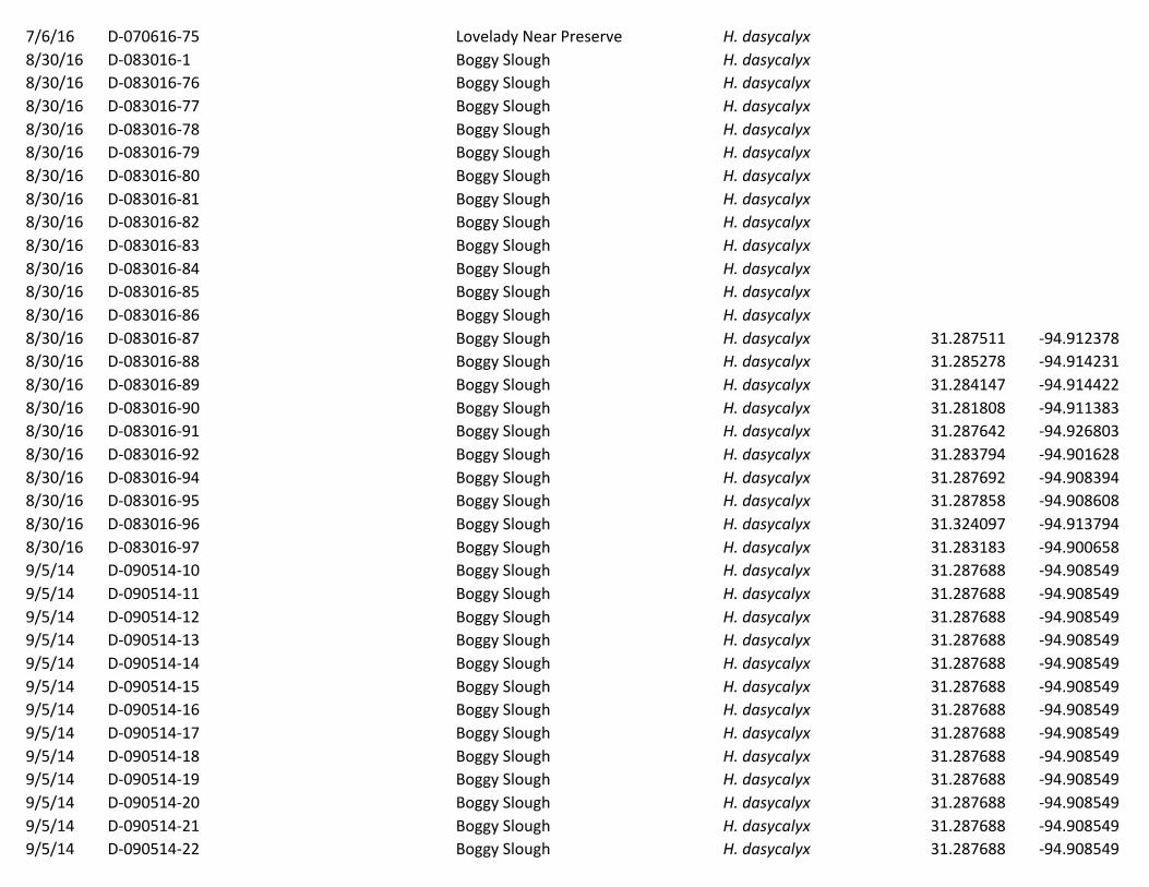
7/6/16 D-070616-75 LoveladyNearPreserve H.dasycalyx 8/30/16 D-083016-1 BoggySlough H.dasycalyx 8/30/16 D-083016-76 BoggySlough H.dasycalyx 8/30/16 D-083016-77 BoggySlough H.dasycalyx 8/30/16 D-083016-78 BoggySlough H.dasycalyx 8/30/16 D-083016-79 BoggySlough H.dasycalyx 8/30/16 D-083016-80 BoggySlough H.dasycalyx 8/30/16 D-083016-81 BoggySlough H.dasycalyx 8/30/16 D-083016-82 BoggySlough H.dasycalyx 8/30/16 D-083016-83 BoggySlough H.dasycalyx 8/30/16 D-083016-84 BoggySlough H.dasycalyx 8/30/16 D-083016-85 BoggySlough H.dasycalyx 8/30/16 D-083016-86 BoggySlough H.dasycalyx 8/30/16 D-083016-87 BoggySlough H.dasycalyx 31.287511 -94.9123788/30/16 D-083016-88 BoggySlough H.dasycalyx 31.285278 -94.9142318/30/16 D-083016-89 BoggySlough H.dasycalyx 31.284147 -94.9144228/30/16 D-083016-90 BoggySlough H.dasycalyx 31.281808 -94.9113838/30/16 D-083016-91 BoggySlough H.dasycalyx 31.287642 -94.9268038/30/16 D-083016-92 BoggySlough H.dasycalyx 31.283794 -94.9016288/30/16 D-083016-94 BoggySlough H.dasycalyx 31.287692 -94.9083948/30/16 D-083016-95 BoggySlough H.dasycalyx 31.287858 -94.9086088/30/16 D-083016-96 BoggySlough H.dasycalyx 31.324097 -94.9137948/30/16 D-083016-97 BoggySlough H.dasycalyx 31.283183 -94.9006589/5/14 D-090514-10 BoggySlough H.dasycalyx 31.287688 -94.9085499/5/14 D-090514-11 BoggySlough H.dasycalyx 31.287688 -94.9085499/5/14 D-090514-12 BoggySlough H.dasycalyx 31.287688 -94.9085499/5/14 D-090514-13 BoggySlough H.dasycalyx 31.287688 -94.9085499/5/14 D-090514-14 BoggySlough H.dasycalyx 31.287688 -94.9085499/5/14 D-090514-15 BoggySlough H.dasycalyx 31.287688 -94.9085499/5/14 D-090514-16 BoggySlough H.dasycalyx 31.287688 -94.9085499/5/14 D-090514-17 BoggySlough H.dasycalyx 31.287688 -94.9085499/5/14 D-090514-18 BoggySlough H.dasycalyx 31.287688 -94.9085499/5/14 D-090514-19 BoggySlough H.dasycalyx 31.287688 -94.9085499/5/14 D-090514-20 BoggySlough H.dasycalyx 31.287688 -94.9085499/5/14 D-090514-21 BoggySlough H.dasycalyx 31.287688 -94.9085499/5/14 D-090514-22 BoggySlough H.dasycalyx 31.287688 -94.908549

9/5/14 D-090514-23 BoggySlough H.dasycalyx 31.287688 -94.9085499/5/14 D-090514-24 BoggySlough H.dasycalyx 31.287688 -94.9085499/5/14 D-090514-4 BoggySlough H.dasycalyx 31.287688 -94.908549;l.... D-090514-5 BoggySlough H.dasycalyx 31.287688 -94.9085499/5/14 D-090514-6 BoggySlough H.dasycalyx 31.287688 -94.9085499/5/14 D-090514-7 BoggySlough H.dasycalyx 31.287688 -94.9085499/5/14 D-090514-8 BoggySlough H.dasycalyx 31.287688 -94.9085499/5/14 D-090514-9 BoggySlough H.dasycalyx 31.287688 -94.9085499/6/14 D-090614-27 BoggySlough H.dasycalyx 31.28261375 -94.901924139/6/14 D-090614-28 BoggySlough H.dasycalyx 31.28261375 -94.901924139/6/14 D-090614-29 BoggySlough H.dasycalyx 31.28261375 -94.901924139/6/14 D-090614-30 BoggySlough H.dasycalyx 31.28261375 -94.901924139/6/14 D-090614-31 BoggySlough H.dasycalyx 31.28261375 -94.901924139/6/14 D-090614-32 BoggySlough H.dasycalyx 31.28261375 -94.901924139/6/14 D-090614-33 BoggySlough H.dasycalyx 31.28261375 -94.901924139/6/14 D-090614-34 BoggySlough H.dasycalyx 31.28261375 -94.901924139/6/14 D-090614-35 BoggySlough H.dasycalyx 31.28261375 -94.901924139/6/14 D-090614-36 BoggySlough H.dasycalyx 31.28261375 -94.901924139/12/14 D-091214-39 MudCreek/Hwy204ROW H.dasycalyx 31.901167 -95.09959/12/14 D-091214-40 MudCreek/Hwy204ROW H.dasycalyx 31.901167 -95.09959/12/14 D-091214-41 MudCreek/Hwy204ROW H.dasycalyx 31.901167 -95.09959/12/14 D-091214-42 MudCreek/Hwy204ROW H.dasycalyx 31.901167 -95.09959/12/14 D-091214-43 MudCreek/Hwy204ROW H.dasycalyx 31.901167 -95.09959/12/14 D-091214-44 MudCreek/Hwy204ROW H.dasycalyx 31.901167 -95.09959/12/14 D-091214-45 MudCreek/Hwy204ROW H.dasycalyx 31.901167 -95.09959/12/14 D-091214-46 MudCreek/Hwy204ROW H.dasycalyx 31.901167 -95.09959/12/14 D-091214-47 MudCreek/Hwy204ROW H.dasycalyx 31.901167 -95.09959/12/16 D-091216-

100 MudCreek H.dasycalyx 31.901042 -95.099389

9/12/16 D-091216-98 MudCreek H.dasycalyx 31.901042 -95.0994649/12/16 D-091216-99 MudCreek H.dasycalyx 31.900628 -95.1014179/28/16 D-092816-

233 BoggySlough H.dasycalyx 31.2807 70'southof-

94.9056910/4/16 D-100416-

235 BoggySlough H.dasycalyx 31.282321 -94.9116

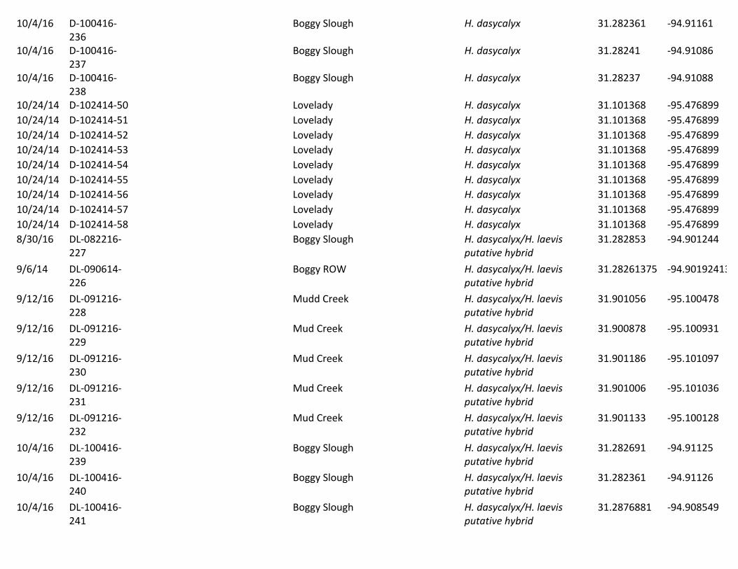
10/4/16 D-100416-236

BoggySlough H.dasycalyx 31.282361 -94.91161

10/4/16 D-100416-237

BoggySlough H.dasycalyx 31.28241 -94.91086

10/4/16 D-100416-238

BoggySlough H.dasycalyx 31.28237 -94.91088

10/24/14 D-102414-50 Lovelady H.dasycalyx 31.101368 -95.47689910/24/14 D-102414-51 Lovelady H.dasycalyx 31.101368 -95.47689910/24/14 D-102414-52 Lovelady H.dasycalyx 31.101368 -95.47689910/24/14 D-102414-53 Lovelady H.dasycalyx 31.101368 -95.47689910/24/14 D-102414-54 Lovelady H.dasycalyx 31.101368 -95.47689910/24/14 D-102414-55 Lovelady H.dasycalyx 31.101368 -95.47689910/24/14 D-102414-56 Lovelady H.dasycalyx 31.101368 -95.47689910/24/14 D-102414-57 Lovelady H.dasycalyx 31.101368 -95.47689910/24/14 D-102414-58 Lovelady H.dasycalyx 31.101368 -95.4768998/30/16 DL-082216-

227 BoggySlough H.dasycalyx/H.laevis

putativehybrid31.282853 -94.901244

9/6/14 DL-090614-226

BoggyROW H.dasycalyx/H.laevisputativehybrid

31.28261375 -94.90192413

9/12/16 DL-091216-228

MuddCreek H.dasycalyx/H.laevisputativehybrid

31.901056 -95.100478

9/12/16 DL-091216-229

MudCreek H.dasycalyx/H.laevisputativehybrid

31.900878 -95.100931

9/12/16 DL-091216-230

MudCreek H.dasycalyx/H.laevisputativehybrid

31.901186 -95.101097

9/12/16 DL-091216-231

MudCreek H.dasycalyx/H.laevisputativehybrid

31.901006 -95.101036

9/12/16 DL-091216-232

MudCreek H.dasycalyx/H.laevisputativehybrid

31.901133 -95.100128

10/4/16 DL-100416-239

BoggySlough H.dasycalyx/H.laevisputativehybrid

31.282691 -94.91125

10/4/16 DL-100416-240

BoggySlough H.dasycalyx/H.laevisputativehybrid

31.282361 -94.91126

10/4/16 DL-100416-241

BoggySlough H.dasycalyx/H.laevisputativehybrid

31.2876881 -94.908549

8/30/16 DM-083016-93

BoggySlough H.dasycalyx/H.moscheutosputativehybrid

31.285564 -94.903625

6/29/14 L-062914-103 DallasAudubonCenter H.laevis 32.703079 -96.7043466/29/14 L-062914-104 dallasAudubonCenter H.laevis 32.703079 -96.7043466/29/14 L-062914-105 dallasAudubonCenter H.laevis 32.70403465 -96.70436046/29/14 L-062914-106 dallasAudubonCenter H.laevis 32.70403465 -96.70436046/29/14 L-062914-107 DallasAudubonCenter H.laevis 32.70403465 -96.70436046/29/14 L-062914-108 DallasAudubonCenter H.laevis 32.704029 -96.7051936/30/14 L-063014-110 HWY24SofCooperJerniganCreek H.laevis 33.32034211 -95.803449376/30/14 L-063014-111 HWY24SofCooperJerniganCreek H.laevis 33.32034211 -95.803449377/29/14 L-072914-113 H.laevis 32.63586 7/29/14 L-072914-114 H.laevis 32.63586 -94.672867/29/14 L-072914-115 H.laevis 32.63586 -94.672867/29/14 L-072914-116 H.laevis 32.63586 -94.672867/29/14 L-072914-117 H.laevis 32.63586 -94.672867/29/14 L-072914-118 H.laevis 32.63586 -94.672867/29/14 L-072914-119 H.laevis 32.63586 -94.672867/29/14 L-072914-120 H.laevis 32.63586 -94.672867/29/14 L-072914-121 H.laevis 32.63586 -94.672867/29/14 L-072914-122 H.laevis 32.63586 -94.672867/29/14 L-072914-123 H.laevis 32.63586 -94.672867/29/14 L-072914-124 H.laevis 32.63586 -94.672867/29/14 L-072914-125 H.laevis 32.63586 -94.672867/29/14 L-072914-126 H.laevis 32.63586 -94.672867/29/14 L-072914-127 H.laevis 32.63586 -94.672867/29/14 L-072914-128 H.laevis 32.63586 -94.672867/29/14 L-072914-129 H.laevis 32.63586 -94.672867/29/14 L-072914-130 H.laevis 32.67161 -94.423317/29/14 L-072914-131 H.laevis 32.67161 -94.423317/29/14 L-072914-132 H.laevis 32.67161 -94.423317/29/14 L-072914-133 H.laevis 32.67161 -94.423317/29/14 L-072914-134 H.laevis 32.67161 -94.423317/29/14 L-072914-135 H.laevis 32.67161 -94.423317/29/14 L-072914-136 H.laevis 32.67161 -94.423317/29/14 L-072914-137 H.laevis 32.67161 -94.42331

7/29/14 L-072914-138 H.laevis 32.67161 -94.423318/12/16 L-081216-152 CypressCreek H.laevis 32.635642 -94.6725928/12/16 L-081216-153 CypressCreek H.laevis 32.635642 -94.6724478/12/16 L-081216-154 CypressCreek H.laevis 32.635117 -94.6729758/12/16 L-081216-155 CypressCreek H.laevis 32.635114 -94.6729978/12/16 L-081216-156 CypressCreek H.laevis 32.635053 -94.6730038/12/16 L-081216-157 CypressCreek H.laevis 32.634936 -94.6728588/12/16 L-081216-158 CypressCreek H.laevis 32.636397 -94.6730338/15/13 L-081513-101 HWY204,MudCreekSite1 H.laevis 31.901167 -95.09958/15/13 L-081513-102 Sideofroad H.laevis 8/22/16 L-082216-144 StrikerCreek H.laevis 32.003478 -94.9904338/22/16 L-082216-145 StrikerCreek H.laevis 32.003522 -94.9904338/22/16 L-082216-146 StrikerCreek H.laevis 32.003161 -94.9920198/22/16 L-082216-147 MudCreek H.laevis 31.855847 -94.9979178/22/16 L-082216-148 MudCreek H.laevis 31.855628 -94.9979088/22/16 L-082216-149 MudCreek&Hwy79 H.laevis 31.976274 -95.1666288/22/16 L-082216-150 StrikerCreek H.laevis 32.003535 -94.9919948/22/16 L-082216-151 MudCreek H.laevis 31.856039 -94.9966510/4/16 L-100416-234 BoggySlough H.laevis 31.282291 -94.914810/22/14 L-102214-141 nearboggyunderbridgeonneches H.laevis 31.286128 -94.891210/22/14 L-102214-142 nearboggyunderbridgeonneches H.laevis 31.286128 -94.891210/22/14 L-102214-143 nearboggyunderbridgeonneches H.laevis 31.2867 -94.8888426/28/14 M-062814-

161 RiverOaksChandlerTX H.moscheutos 32.313542 -95.46005

6/28/14 M-062814-162

sideofroadChandlerTX H.moscheutos 32.312607 -95.460385

7/22/14 M-072214-164

Hwy69SoutofTyler H.moscheutos 32.14039887 -95.31127378

7/22/14 M-072214-165

Hwy69SoutofTyler H.moscheutos 32.14039887 -95.31127378

7/29/14 M-072914-166

LammySiteHarrisonCnty H.moscheutos 32.62743 -94.51598

7/29/14 M-072914-167

LammySiteHarrisonCnty H.moscheutos 32.62743 -94.51598

7/29/14 M-072914-168

LammySiteHarrisonCnty H.moscheutos 32.62743 -94.51598

7/29/14 M-072914-169

LammySiteHarrisonCnty H.moscheutos 32.62743 -94.51598

7/29/14 M-072914-170

LammySiteHarrisonCnty H.moscheutos 32.62743 -94.51598

7/29/14 M-072914-171

LammySiteHarrisonCnty H.moscheutos 32.62743 -94.51598

7/29/14 M-072914-172

LammySiteHarrisonCnty H.moscheutos 32.62743 -94.51598

7/29/14 M-072914-173

LammySiteHarrisonCnty H.moscheutos 32.62743 -94.51598

7/29/14 M-072914-174

LammySiteHarrisonCnty H.moscheutos 32.62743 -94.51598

7/29/14 M-072914-175

LammySiteHarrisonCnty H.moscheutos 32.62743 -94.51598

7/29/14 M-072914-176

LammySiteHarrisonCnty H.moscheutos 32.62743 -94.51598

7/29/14 M-072914-177

LammySiteHarrisonCnty H.moscheutos 32.62743 -94.51598

7/29/14 M-072914-178

LammySiteHarrisonCnty H.moscheutos 32.62743 -94.51598

7/29/14 M-072914-179

LammySiteHarrisonCnty H.moscheutos 32.62743 -94.51598

7/29/14 M-072914-180

LammySiteHarrisonCnty H.moscheutos 32.62743 -94.51598

7/29/14 M-072914-181

LammySiteHarrisonCnty H.moscheutos 32.62743 -94.51598

7/29/14 M-072914-182

LammySiteHarrisonCnty H.moscheutos 32.62743 -94.51598

7/29/14 M-072914-183

LammySiteHarrisonCnty H.moscheutos 32.62743 -94.51598

7/29/14 M-072914-184

LammySiteHarrisonCnty H.moscheutos 32.62743 -94.51598

7/29/14 M-072914-185

LammySiteHarrisonCnty H.moscheutos 32.62743 -94.51598

7/29/14 M-072914-186

LammySiteHarrisonCnty H.moscheutos 32.62743 -94.51598

7/29/14 M-072914-187

LammySiteHarrisonCnty H.moscheutos 32.62743 -94.51598

7/29/14 M-072914-188

LammySiteHarrisonCnty H.moscheutos 32.678896 -94.502723

7/29/14 M-072914-189

LammySiteHarrisonCnty H.moscheutos 32.678896 -94.502723

7/29/14 M-072914-190

LammySiteHarrisonCnty H.moscheutos 32.678896 -94.502723

7/29/14 M-072914-191

LammySiteHarrisonCnty H.moscheutos 32.678896 -94.502723

7/29/14 M-072914-192

LammySiteHarrisonCnty H.moscheutos 32.678896 -94.502723

7/29/14 M-072914-193

ROWHarrisonCnty H.moscheutos 32.615227 -94.580391

8/16/14 M-081614-194

aroundpondTNHwy54 H.moscheutos 35.58216476 -89.42619323

8/16/14 M-081614-195

aroundpondTNHwy54 H.moscheutos 35.58216476 -89.42619323

8/16/14 M-081614-196

aroundpondTNHwy54 H.moscheutos 35.58216476 -89.42619323

8/16/14 M-081614-197

aroundpondTNHwy54 H.moscheutos 35.58216476 -89.42619323

8/16/14 M-081614-198

aroundpondTNHwy54 H.moscheutos 35.58216476 -89.42619323

8/16/14 M-081614-199

aroundpondTNHwy54 H.moscheutos 35.58216476 -89.42619323

8/16/14 M-081614-200

aroundpondTNHwy54 H.moscheutos 35.58216476 -89.42619323

8/16/14 M-081614-201

aroundpondTNHwy54 H.moscheutos 35.58216476 -89.42619323

8/16/14 M-081614-202

aroundpondTNHwy54 H.moscheutos 35.58216476 -89.42619323

8/16/14 M-081614-203

aroundpondTNHwy54 H.moscheutos 35.58216476 -89.42619323

8/16/14 M-081614-204

ROWTNHwy54 H.moscheutos 35.56882095 -89.48236083

8/16/14 M-081614-205

ROWTNHwy54 H.moscheutos 35.56882095 -89.48236083

8/16/14 M-081614-206

ROWTNHwy54 H.moscheutos 35.56882095 -89.48236083

8/16/14 M-081614-207

ROWTNHwy54 H.moscheutos 35.56882095 -89.48236083

8/16/14 M-081614-208

ROWTNHwy54 H.moscheutos 35.56882095 -89.48236083

8/16/14 M-081614-209

ROWTNHwy54 H.moscheutos 35.56882095 -89.48236083

8/16/14 M-081614-210

ROWTNHwy54 H.moscheutos 35.56882095 -89.48236083

8/16/14 M-081614-211

ROWTNHwy54 H.moscheutos 35.56882095 -89.48236083

8/16/14 M-081614-212

ROWTNHwy54 H.moscheutos 35.56882095 -89.48236083

8/16/14 M-081614-213

ROWTNHwy54 H.moscheutos 35.56882095 -89.48236083

8/16/14 M-081614-214

ROWTNHwy54 H.moscheutos 35.56882095 -89.48236083

8/16/14 M-081614-215

ROWTNHwy54 H.moscheutos 35.56882095 -89.48236083

8/16/14 M-081614-216

ROWTNHwy54 H.moscheutos 35.56882095 -89.48236083

8/16/14 M-081614-217

ROWTNHwy54 H.moscheutos 35.56882095 -89.48236083

8/16/14 M-081614-218

ROWTNHwy54 H.moscheutos 35.56882095 -89.48236083

8/16/14 M-081614-219

ROWTNHwy54 H.moscheutos 35.56882095 -89.48236083

8/16/14 M-081614-220

ROWTNHwy54 H.moscheutos 35.56882095 -89.48236083

8/16/14 M-081614-221

ROWTNHwy54 H.moscheutos 35.56882095 -89.48236083

8/16/14 M-081614-222

ROWTNHwy54 H.moscheutos 35.56882095 -89.48236083

8/30/16 M-083016-223

BoggySlough H.moscheutos 31.319381 -94.927008

9/12/16 M-091216-225

MudCreek/Hwy204ROW H.moscheutos 31.901056 -95.100478

9/17/13 M-091713-159

BoggySlough H.moscheutos 31.282667 -94.902

9/17/13 M-091713-160

BoggySlough H.moscheutos 31.282667 -94.902

9/27/16 M-092716-224

MudCreekHwy110 H.moscheutos 32.162522 -95.171586

Table3.Theplantsamplesusedforanalysisofmolecularvariance(AMOVA)ofGBSSItoderiveFSTvalues.Foreachplantsample(rows),thedesignationsofwhichpopulationtheybelongedto,aswellastheirgeneticidentificationnumbers(columns),areprovided.

Species Population# Identification#H.dasycalyx 1 D48H.dasycalyx 1 D49H.dasycalyx 2 D2H.dasycalyx 2 D24H.dasycalyx 2 D25H.dasycalyx 3 D37H.dasycalyx 3 D38H.laevis 4 L11H.laevis 4 L12H.laevis 5 L10H.laevis 5 L6H.laevis 5 L7H.laevis 5 L4H.laevis 5 L5H.laevis 6 L59H.laevis 6 L60H.laevis 7 L1H.laevis 7 L40H.laevis 7 L41H.laevis 8 L14H.laevis 8 L15H.laevis 8 L31H.laevis 8 L32H.moscheutos 9 M5H.moscheutos 9 M6H.moscheutos 10 M8H.moscheutos 10 M9H.moscheutos 11 M10H.moscheutos 11 M11H.moscheutos 11 M32H.moscheutos 11 M33H.moscheutos 11 M37H.moscheutos 12 M38H.moscheutos 12 M39H.moscheutos 12 M48H.moscheutos 12 M49

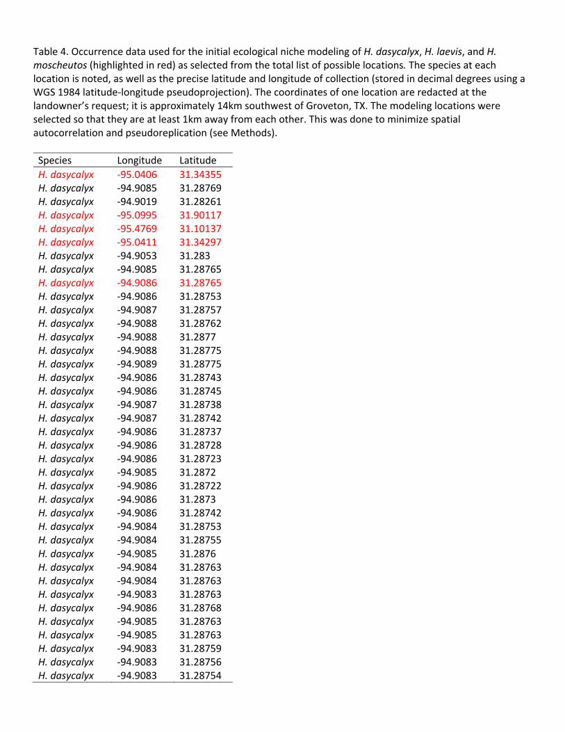
Table4.OccurrencedatausedfortheinitialecologicalnichemodelingofH.dasycalyx,H.laevis,andH.moscheutos(highlightedinred)asselectedfromthetotallistofpossiblelocations.Thespeciesateachlocationisnoted,aswellasthepreciselatitudeandlongitudeofcollection(storedindecimaldegreesusingaWGS1984latitude-longitudepseudoprojection).Thecoordinatesofonelocationareredactedatthelandowner’srequest;itisapproximately14kmsouthwestofGroveton,TX.Themodelinglocationswereselectedsothattheyareatleast1kmawayfromeachother.Thiswasdonetominimizespatialautocorrelationandpseudoreplication(seeMethods).Species Longitude LatitudeH.dasycalyxH.dasycalyx

-95.0406-94.9085

31.3435531.28769

H.dasycalyx -94.9019 31.28261H.dasycalyx -95.0995 31.90117H.dasycalyx -95.4769 31.10137H.dasycalyx -95.0411 31.34297H.dasycalyx -94.9053 31.283H.dasycalyx -94.9085 31.28765H.dasycalyx -94.9086 31.28765H.dasycalyx -94.9086 31.28753H.dasycalyx -94.9087 31.28757H.dasycalyx -94.9088 31.28762H.dasycalyx -94.9088 31.2877H.dasycalyx -94.9088 31.28775H.dasycalyx -94.9089 31.28775H.dasycalyx -94.9086 31.28743H.dasycalyx -94.9086 31.28745H.dasycalyx -94.9087 31.28738H.dasycalyx -94.9087 31.28742H.dasycalyx -94.9086 31.28737H.dasycalyx -94.9086 31.28728H.dasycalyx -94.9086 31.28723H.dasycalyx -94.9085 31.2872H.dasycalyx -94.9086 31.28722H.dasycalyx -94.9086 31.2873H.dasycalyx -94.9086 31.28742H.dasycalyx -94.9084 31.28753H.dasycalyx -94.9084 31.28755H.dasycalyx -94.9085 31.2876H.dasycalyx -94.9084 31.28763H.dasycalyx -94.9084 31.28763H.dasycalyx -94.9083 31.28763H.dasycalyx -94.9086 31.28768H.dasycalyx -94.9085 31.28763H.dasycalyx -94.9085 31.28763H.dasycalyx -94.9083 31.28759H.dasycalyx -94.9083 31.28756H.dasycalyx -94.9083 31.28754

H.dasycalyx -94.9083 31.28758H.dasycalyx -94.9084 31.28761H.dasycalyx -94.9084 31.28753H.dasycalyx -94.9084 31.28755H.dasycalyx -94.9085 31.28714H.dasycalyx -94.9084 31.28701H.dasycalyx -94.9087 31.28741H.dasycalyx -94.9087 31.28741H.dasycalyx -94.9087 31.28743H.dasycalyx -94.9087 31.28747H.dasycalyx -94.9087 31.28747H.dasycalyx -94.9086 31.28766H.dasycalyx -94.9083 31.2878H.dasycalyx -94.9054 31.28303H.dasycalyx -94.9017 31.28453H.dasycalyx -94.9022 31.28498H.dasycalyx -94.9022 31.285H.dasycalyx -94.9024 31.285H.dasycalyx -94.9027 31.28504H.dasycalyx -94.9027 31.28516H.dasycalyx -94.9027 31.28505H.dasycalyx -94.9027 31.28501H.dasycalyx -94.9027 31.28501H.dasycalyx -94.9026 31.28525H.laevis Redacted RedactedH.laevis -95.0995 31.90117H.laevis -96.7043 32.70308H.laevis -96.7044 32.70435H.laevis -96.7052 32.70403H.laevis -96.7044 32.70323H.laevis -95.8034 33.32034H.laevis -95.2846 31.62904H.laevis -94.6729 32.63586H.laevis -94.4233 32.67161H.laevis -95.57 33.65111H.laevis -95.5287 30.92031H.laevis -94.08 30.5H.laevis -94.751 32.67313H.laevis -95.6211 29.36615H.laevis -94.8888 31.2867H.laevis -95.1895 32.54451H.laevisH.laevisH.laevisH.laevis

-94.8912-95.364182-94.901721-95.102199

31.2861331.13727431.28269431.900913

H.moscheutos -94.902 31.28267H.moscheutos -95.4601 32.31354

H.moscheutos -95.4604 32.31261H.moscheutos -95.4583 32.58368H.moscheutos -95.3113 32.1404H.moscheutos -94.516 32.62743H.moscheutos -94.5027 32.6789H.moscheutos -94.5804 32.61523H.moscheutos -94.8986 31.2825H.moscheutos -95.7781 29.1225H.moscheutos -93.9019 30.26028H.moscheutos -94.3772 29.625H.moscheutos -94.3737 29.67281H.moscheutos -93.7946 30.55082H.moscheutos -95.3174 32.20589H.moscheutos -94.5156 32.62784H.moscheutos -94.5952 32.60126H.moscheutos -94.7935 32.46132H.moscheutos -94.3193 33.03356H.moscheutos -94.1879 32.69605H.moscheutos -94.9304 31.31666

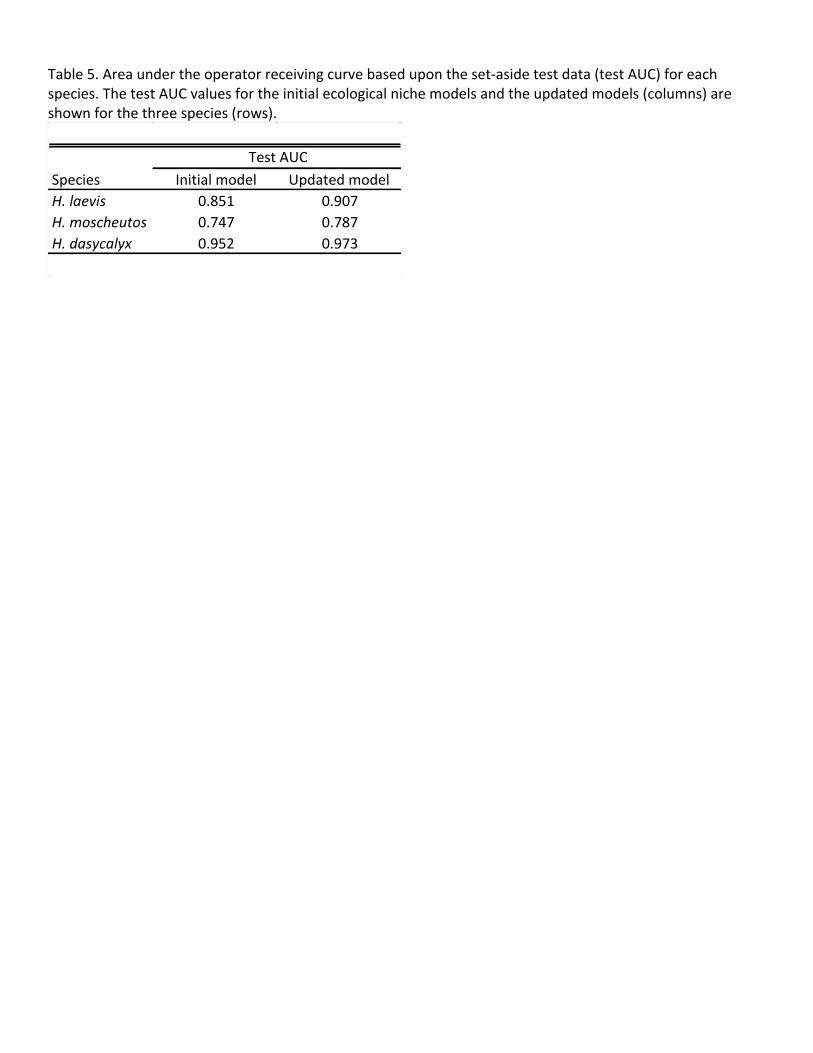
Table5.Areaundertheoperatorreceivingcurvebasedupontheset-asidetestdata(testAUC)foreachspecies.ThetestAUCvaluesfortheinitialecologicalnichemodelsandtheupdatedmodels(columns)areshownforthethreespecies(rows).

Species Initialmodel UpdatedmodelH.laevis 0.851 0.907H.moscheutos 0.747 0.787H.dasycalyx 0.952 0.973

TestAUC

Table6.Ground-truthlocationsforH.laevis(rows).Incolumns,theGPScoordinatesofeachlocationareprovided(storedindecimaldegreesusingaWGS1984latitude-longitudepseudoprojection),aswellasthehabitatsuitabilitythatwaspredictedforthatlocation(Suitability)andwhetherthespecieswasfoundthereornot(Present?).

Longitude Latitude Suitability Present?-94.990433 32.003478 0.785971 Yes-94.997917 31.855847 0.785971 Yes-95.166628 31.976274 0.785971 Yes-95.163078 32.158806 0.822833 No-95.106658 31.885711 0.00424675 No-95.16185 31.897114 0.00424675 No-95.129081 31.911231 0.785971 No-94.910179 32.197902 0.00832754 No-96.256592 32.733667 0.156597 No-94.9635 32.52625 0.391538 No-95.485231 32.611242 0.574521 No

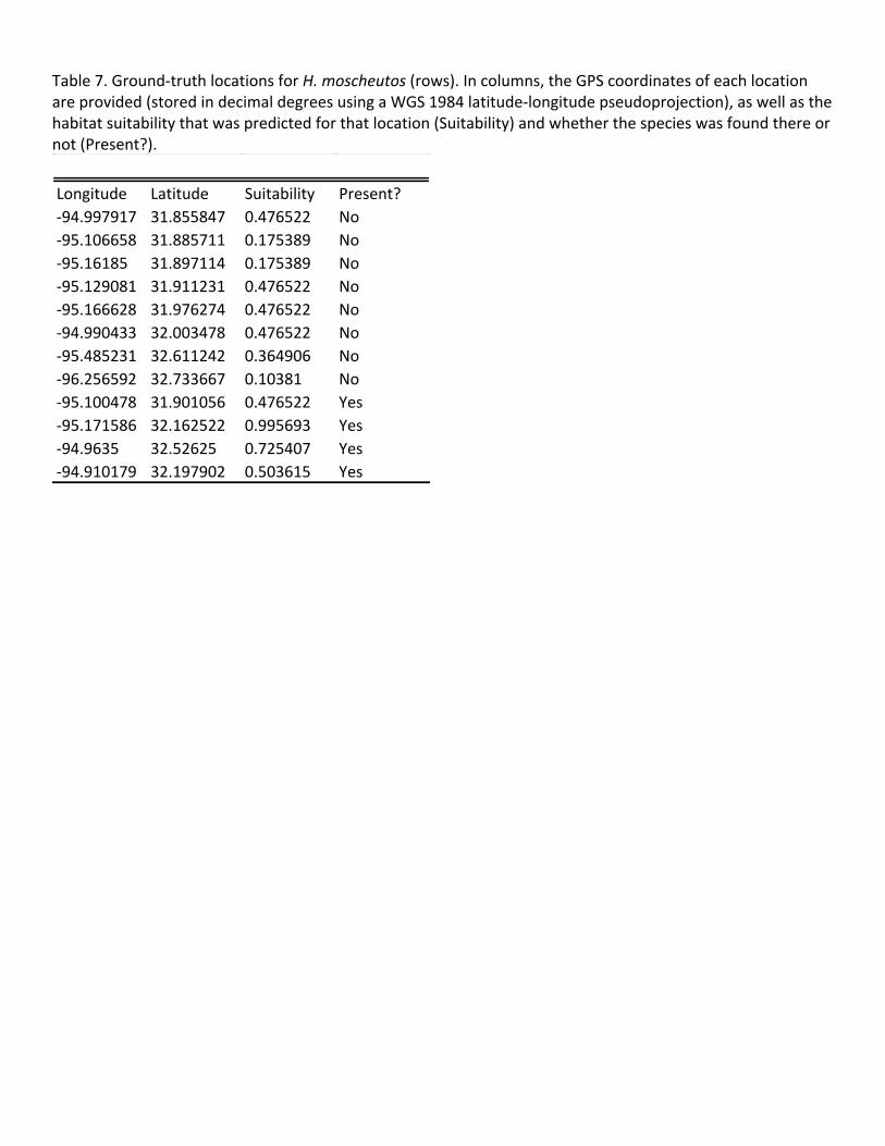
Table7.Ground-truthlocationsforH.moscheutos(rows).Incolumns,theGPScoordinatesofeachlocationareprovided(storedindecimaldegreesusingaWGS1984latitude-longitudepseudoprojection),aswellasthehabitatsuitabilitythatwaspredictedforthatlocation(Suitability)andwhetherthespecieswasfoundthereornot(Present?).

Longitude Latitude Suitability Present?-94.997917 31.855847 0.476522 No-95.106658 31.885711 0.175389 No-95.16185 31.897114 0.175389 No-95.129081 31.911231 0.476522 No-95.166628 31.976274 0.476522 No-94.990433 32.003478 0.476522 No-95.485231 32.611242 0.364906 No-96.256592 32.733667 0.10381 No-95.100478 31.901056 0.476522 Yes-95.171586 32.162522 0.995693 Yes-94.9635 32.52625 0.725407 Yes-94.910179 32.197902 0.503615 Yes

Table8.Ground-truthlocationsforH.dasycalyx(rows).Incolumns,theGPScoordinatesofeachlocationareprovided(storedindecimaldegreesusingaWGS1984latitude-longitudepseudoprojection),aswellasthehabitatsuitabilitythatwaspredictedforthatlocation(Suitability)andwhetherthespecieswasfoundthereornot(Present?).

Longitude Latitude Suitability Present?-94.990433 32.003522 0.826178 No-94.997917 31.855847 0.826178 No-95.166628 31.976274 0.826178 No-95.163078 32.158806 0.772046 No-95.106658 31.885711 0.00026805 No-95.16185 31.897114 0.00026805 No-95.129081 31.911231 0.826178 No-94.910179 32.197902 0.00038363 No-96.256592 32.733667 1.55E-07 No-94.9635 32.52625 0.164213 No-95.485231 32.611242 0.224171 No-94.914422 31.284147 0.659131 Yes-94.926803 31.287642 0.659131 Yes-94.902608 31.2852469 0.857051 Yes-94.913794 31.324097 0.857051 Yes

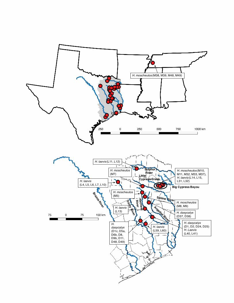
H. laevis (L11, L12)

H. moscheutos (M10, M11, M32, M33, M37),H. laevis (L14, L15, L31, L32)

H. moscheutos(M7)

H. laevis(L4, L5, L6, L7, L10)

H. moscheutos(M5)

H. moscheutos(M8, M9)

H. dasycalyx(D37, D38)

H. laevis(L13)

H. dasycalyx(D1, D2, D24, D25)H. Laevis(L40, L41)

H. dasycalyx(D1c, D5a, D6b, D8, D9b, D11, D48, D49)

H. laevis(L59, L60)

Big Cypress Bayou

SulphurRiver

LittleCypress Creek

H. moscheutos (M38, M39, M48, M49)

Figure1.Locationsofthepopulationsusedinthegeneticanalyses(redcircles).Theidentificationnumbersinparenthesesrefertospecificplantsthatwereusedforgeneticanalysis(seeTable1).ThemajorriversinEastTexasareindicatedinblue.ThenamesoftheEastTexasrivers,aswellastheEastTexascountyboundaries(blacklines),areprovided.

Figure2.(a)RootedmaximumlikelihoodtreeshowingphylogeneticrelationshipsofH.dasycalyx,H.laevis,andH.moscheutosinferredfromGBSSIintronsequences,withproportionalbranchlengths.Whenheterozygoteswerepresent,eachphasedallelewasanalyzedseparatelyasifitwereaseparateindividual.Allelesareindicatedby“-1”and“-2”suffixes.Bootstrapvaluesgreaterthan50%areshownateachnode.Eachindividual(tip)islabeledbyspecies.DrepresentsH.dasycalyx,LrepresentsH.laevis,MrepresentsH.moscheutos,RDrepresentsanH.dasycalyxindividualfromSmall(2004),andTrepresentstheoutgroupH.trionum.Theslashontheoutgroupbranchindicatesthatthelengthhasbeenshortenedforvisualizationpurposes.(b)Thesamephylogeny,butwithoutproportionalbranchlengthssothatcladesaremoreeasilyvisible.

M11-2M11-1

M32-2M10-2

M37-1

M8-2M6-1M7-1M5-2

M23-1M6-2M7-2M8-1M10-1M33-2M33-1M49-1

M49-2M48-2M39-1M39-2M38-2M38-1

M48-1M37-2M9-1M5-1M9-2

T

D38-2D48-2D48-1D49-2

L15L31L32

L14RD-2

D49-1

D38-1D24-2D25-1D25-2D24-1D2-1

D37-2RD-1

L41L40L13L12L11L10L7L6L5L4L60L59D37-1D2-2D1-2D1-1

77

8458

58

53

52

62

78 74

56

55

64

/

0.001

M11-2M11-1M32-2M10-2M37-1

M8-2M6-1M7-1M5-2M23-1M6-2M7-2M8-1M10-1M33-2M33-1M49-1M49-2M48-2M39-1M39-2M38-2M38-1M48-1M37-2M9-1M5-1M9-2

T

D38-2D48-2D48-1D49-2L15L31L32L14RD-2D49-1

D38-1D24-2D25-1D25-2D24-1D2-1

D37-2RD-1

L41L40L13L12L11L10L7L6L5L4L60L59D37-1D2-2D1-2D1-1

77

845858

53

52

62

7874

56

55

64

a b

Gro

up II

Gro

up I

H. laevis clade

H. dasycalyxclade

H. laevis clade

Figure3.RootedmaximumlikelihoodtreeshowingphylogeneticrelationshipsofH.dasycalyx,H.laevis,andH.moscheutosinferredfromthegenome-widedata.Bootstrapvaluesgreaterthan60%areshownoneachbranch.EachaccessionislabeledbyspeciesDrepresentH.dasycalyx,LrepresentsH.laevis,MrepresentsH.moscheutos,andT1representstheoutgroupH.trionum.

Gro

up II

Gro

up I

Figure4.RootedBayesiancoalescencetreeshowingphylogeneticrelationshipsofH.dasycalyx,H.laevis,andH.moscheutosinferredfromthegenome-widedata.Posteriorsupportvaluesgreaterthan0.7areshownaboveeachbranch.Eachaccessionislabeledbyspecies.DrepresentsH.dasycalyx,LrepresentsH.laevis,MrepresentsH.moscheutos,andT1representstheoutgroupH.trionum.

Gro

up II

Gro

up I

Figure5.AgraphicalrepresentationoftheBayesianclusteranalysisoftheGBSSIsequencedata,showingthepercentagesofdifferentinferredancestries(y-axis)comprisingeachindividual(x-axis).Thedifferentinferredancestralgroupsarecolor-codedblue,red,yellow,green,andpurple.DrepresentsH.dasycalyx,LrepresentsH.laevis,MrepresentsH.moscheutos,andRDrepresentsanH.dasycalyxindividualfromSmall(2004).

Figure6.AgraphicalrepresentationoftheBayesianclusteranalysisofthegenome-widedata,showingthepercentagesofdifferentinferredancestries(y-axis)comprisingeachindividual(x-axis).Thedifferentinferredancestralgroupsarecolor-codedgreenandpurple.DrepresentsH.dasycalyx,LrepresentsH.laevis,andMrepresentsH.moscheutos.

D11D1cD5aD6bD8D9bL11L15L31L41M10M11M37M38M7

100%

90%

80%

70%

60%

50%

40%

30%

20%

10%

0

Figure7.AgraphicalrepresentationoftheBayesianclusteranalysisofthegenome-widedata,showingthepercentagesofdifferentinferredancestries(y-axis)comprisingeachindividual(x-axis).Thedifferentinferredancestralgroupsarecolor-codedred,blue,peagreen,black,orange,andgreen.DrepresentsH.dasycalyxandLrepresentsH.laevis.H.moscheutosisexcluded.

100%

90%

80%

70%

60%

50%

40%

30%

20%

10%

0D1cD11D5aD8D9bD6bL11L31 L15L41

Figure8.Inblue:countieswithexistingdocumentednativepopulationsofH.dasycalyxinEastTexas:Cherokee,Houston,andTrinity.Inbeige:countiesincludedintheecologicalnichemodelinganalyses.

H. laevisH. laevis

H. moscheutos

H. moscheutos,H. laevis

H. moscheutos

H. moscheutosH. laevis

H. moscheutos

H. moscheutos

H. dasycalyxH. laevis

H. dasycalyxH. Laevis

H. laevis

H. dasycalyx

H. laevis

H. laevis

H. moscheutos

H. moscheutos

Big Cypress Bayou

SulphurRiver

LittleCypress Creek

Figure9.Locationsofthepopulationsusedintheinitialecologicalnichemodelingofthethreespecies(redcircles).ThemajorriversinEastTexasareindicatedinblue.ThenamesoftheEastTexasrivers,aswellastheEastTexascountyboundaries(blacklines),areprovided.

H. laevis

H. moscheutos

Figure10.Ground-truthlocationsthatweresearchedforthethreespecies(redcircles).Thelocationswhereplantswerefoundareindicatedwitharrowsandlabels.ThemajorriversinEastTexasareindicatedinblue.ThenamesoftheEastTexasrivers,aswellastheEastTexascountyboundaries(blacklines),areprovided.

Figure11.Ground-truthingoftheinitialecologicalnichemodelsforeachofthethreespecies.Thewhitecolumnsrepresenttheaveragehabitatsuitability(fromtheecologicalnichemodel)ofthelocationswherethespecieswasnotfound.Thegreycolumnsrepresenttheaveragehabitatsuitabilityofthelocationswherethespecieswasfound.Thebarsrepresent±1SE.Foreachspecies,theP-valuesfromtheStudent’st-testandthelikelihoodratio(LR)testarepresented,indicatingwhetherornotthedifferenceinhabitatsuitabilitybetweentheabsenceandpresencelocationswassignificant.

Figure12.HabitatsuitabilityforH.laevisacrossEastTexas,asforecastbytheupdatedecologicalnichemodelthatincludestheground-truthingdata.Thecolorsonthelandscaperepresentthehabitatsuitabilityatthatlocationatagransizeof100mx100m.Habitatsuitabilitiesarecolorcodedfromzerotoone,withzerobeingtheleastsuitablehabitatandonebeingthemostsuitablehabitat.TheEastTexascountyboundariesareoutlinedinblackforcontext.Whitespacesindicatemissingdata.

Figure13.HabitatsuitabilityforH.moscheutosacrossEastTexas,asforecastbytheupdatedecologicalnichemodelthatincludestheground-truthingdata.Thecolorsonthelandscaperepresentthehabitatsuitabilityatthatlocationatagransizeof100mx100m.Habitatsuitabilitiesarecolorcodedfromzerotoone,withzerobeingtheleastsuitablehabitatandonebeingthemostsuitablehabitat.TheEastTexascountyboundariesareoutlinedinblackforcontext.Whitespacesindicatemissingdata.

Figure14.HabitatsuitabilityforH.dasycalyxacrossEastTexas,asforecastbytheupdatedecologicalnichemodelthatincludestheground-truthingdata.Thecolorsonthelandscaperepresentthehabitatsuitabilityatthatlocationatagransizeof100mx100m.Habitatsuitabilitiesarecolorcodedfromzerotoone,withzerobeingtheleastsuitablehabitatandonebeingthemostsuitablehabitat.TheEastTexascountyboundariesareoutlinedinblackforcontext.Whitespacesindicatemissingdata.

Figure15.Averagehabitatsuitabilitythethreespeciesintermsof(a)calciumcarbonateconcentration,(b)erodibility,(c)liquidlimitofthesoillayer,(d)slopeofthemapunit,and(e)depthtotheseasonally-highwatertable.TheredlineisH.laevis,thegreenlineisH.moscheutos,andtheredlineisH.dasycalyx.