final report intercomparison campaign final version

Intercomparison campaign (WP3.4)

Final Report

March 2012

2

www.apice-project.eu

Colophon Title:

Intercomparison campaign (WP3.4): final Report Subtitle: APICE WP 3.4 Main Author(s): A. Detournay1, J. Pey2, N. Perez2, M.C. Bove3, V. Ariola3, E. Cuccia3, D. Massabò3, P. Prati3, J.G. Bartzis4, D. Saraga4, E. Tolis4 , K. Filiou4, A. Latella5, A. De Bortoli5, F. Liguori5, S. Patti5, N. Marchand1

(1) Aix Marseille Univ, CNRS, Laboratoire Chimie Environnement-Instrumentation et Réactivité Atmosphérique, Marseille, France.

(2) Institute of Environmental Assessment and Water Research (IDAEA-CSIC), Barcelona, Spain. (3) University of Genoa - Department of Physics, via Dodecaneso 33, 16146, Genova, Italy

(4)University of West Macedonia, Kozani, Greece (5) ARPA Veneto, Padova, Italy

Responsible institution(s): Aix Marseille Univ, CNRS, Laboratoire Chimie Environnement-Instrumentation et Réactivité Atmosphérique (N. Marchand) Language: English Keywords: Harbors, Industry, Marseille, Aerosol, Source apportionment, chemical composition, Intercomparison.

3


Content Abstract .....................................................................................................................4

1. Introduction.....................................................................................................5 2. Overview of the field campaign conditions .....................................................6

2.1. Sampling site and measurements ...........................................................6 2.2. Field campaign conditions.......................................................................8

3. Summary of the intercomparison of measurements .....................................11 4. Source apportionment intercomparison........................................................14

4.1. PMF and CMB general description........................................................14 4.2. Methodology used by each partners .....................................................16 4.3. Intercomparison of source apportionment approaches .........................19

5. Conclusions and perspectives......................................................................24 6. References ...................................................................................................25

Appendix I : Intercomparison of organic markers ....................................................27 Appendix II.1 : Source apportionment results (IDAEA-CSIC, Barcelona)................31

1. Identification of emission sources.................................................................31 2. Quantification of source contributions ..........................................................33 3. Temporal trends ...........................................................................................35

Appendix II.2 : Source apportionment results (Univ Genoa, Genoa).......................37 1. Methodology of sampling and methods of analysis ......................................37 2. Source apportionment approach ..................................................................38 3. Results .........................................................................................................40

Appendix II.3 : Source apportionment results (Univ. Provence, Marseille)..............46 1. CMB modeling set up ...................................................................................46

1.1. CMB modeling: Definition......................................................................46 1.2. Choice of profile sources and Markers..................................................46 1.3. Quality control .......................................................................................48

2. Estimate of sea salts and crustal dust apportionment ..................................48 2.1. Sea salt .................................................................................................49 2.2. Crustal dust ...........................................................................................49 2.3. Contribution to PM 2.5...........................................................................49

3. CMB modeling results ..................................................................................51 3.1. Primary sources contribution assessed by the CMB .............................51

3.1.1. Sources contribution to PM 2.5 ........................................................52 4. PM2.5 average composition .........................................................................53 5. Conclusion....................................................................................................55

Appendix II.4 : Source apportionment results (UOWM, Thessaloniki).....................57 1. Introduction...................................................................................................57 2. Methodology.................................................................................................57

2.1. Available data from chemical analysis...................................................57 2.2. Data pre-treatment and analysis of input data.......................................58 2.3. Statistical parameters............................................................................58

3. Results and discussion.................................................................................58 Appendix II.5 : Source apportionment results (IDAEA-CSIC/U. Genoa, Venice).....64

1. Source apportionment approach ..................................................................64

4


Abstract

Assessing the source contributions of PM by a top down approach requires advanced

analytical and statistical approaches. Because no absolute source apportionment approach exists,

intercomparison of the different methodologies used by each scientific partners of APICE is a

prerequisite for any comparison between the 5 harbors (Barcelona, Genoa, Marseille, Thessaloniki

and Venice) involved in the project.

A six weeks intercomparison campaign was organized in Marseille from the 25th of January

to the 2nd of March 2011 in an urban background site. The objectives of this field campaign were

to intercompare airborne measurements (mass, chemical composition) and source apportionment

methodologies in order to converge towards a common methodology.

Regarding measurements, whereas OC, K/K+ and SO4

2- in the PM2.5 fraction resulted in very

similar concentrations and temporal evolution for all the partners, some other major components,

such as Ca/Ca2+

, Mg/Mg2+

and NO3-, show significant differences for at least one partner. This can

be explained by minor analytical and non permanent problems (ie: calibration, contamination).

Raw data and analytical conditions will be checked by the partner for whom the data set appears

problematic for at least one point. For minor fraction (metals and elements) we observe good

agreement, within classical analytical error range, for the most relevant source markers (Pb, Fe,

Cu, Zn, Ni).

Regarding source apportionment methodologies, each partner was free to use his own

one (measurements and source apportionment model). As expected, significant discrepancies are

observed. However these discrepancies regard mostly the average contribution of some sources

while the temporal trends are in fair agreements. Differences can also be linked quite easily to the

methodology used, either regarding the choice of fitting species or source profiles, either

considering biases induced by the dynamic of the atmosphere (particularly important considering

the number of observations).

In order to converge towards a homogenous methodology between each pilot area, our

recommendations are as follows:

1/ Use of the same source apportionment approach. The source apportionment approach

chosen is PMF (Positive Matrix Factorization). In consequence, Aix Marseille Univ will also use PMF

in addition to CMB,

2/ Use of a common basis of chemical markers as fitting species. The chemical markers list

will include trace elements/metals and organic markers or at least the different carbon fractions

(OC1, OC2,.., Pyrolitic Carbon), in addition to OC, EC, sulfate, nitrate and ammonium. The list of

chemical markers will be defined by the partnership after a careful study of the chemical data

obtained during the long monitoring campaigns. Some additional markers may be added to the list

in each pilot area in order to take into account the specificity of each pilot area,

3/ Common interpretation of the different factors identified in each pilot area.

5


1. Introduction

Source apportionment of atmospheric particulate matter (PM) is far from a

straightforward exercise. Atmospheric aerosol consists of a highly complex mixture, in constant

evolution in the atmosphere, of mineral and organic materials associated to micron and

submicron particles. In urban areas, atmospheric aerosols are emitted to the atmosphere by a

multitude of sources and also formed in situ through gas phase oxidation processes of volatile

organic compounds (VOC) or gases such as SO2, NOx. Assessing the source contributions of PM by

a top down approach requires advanced analytical and statistical approaches. Because no absolute

source apportionment approach exists, intercomparison of the different methodologies used by

each scientific partners of APICE is a prerequisite for any comparison between the 5 harbors

(Barcelona, Genoa, Marseille, Thessaloniki and Venice) involved in the project.

A six weeks intercomparison campaign was organized in Marseille from the 25th of January

to the 2nd of March 2011 in an urban background site. The objectives of this field campaign were

to intercompare measurements and source apportionment methodologies in order to converge

towards a common methodology. The intercomparison campaign gathers all the scientific partners

involved in the measurements and source apportionment task. Several instruments were

deployed including state of the art instruments such as Aerosol Mass Spectrometer (AMS) for

online monitoring of non-refractory submicron particles composition and Proton Transfert

Reaction Mass Spectrometer (PTR-MS) for online monitoring of VOCs. Initially planned in autumn

2010, the field campaign was delayed to February/March 2011 for logistical issues and to

guarantee its success. A first report discussing of the intercomparison of measurements has been

already published1.

The present report summarizes the campaign conditions and the intercomparison of

chemical markers measurements used as fitting species in each source apportionment approach.

This report focuses on the intercomparison of source apportionment exercise performed by each

partner and proposes recommendations to converge towards a common and concerted

methodology. Complete source apportionments description and results are presented in Appendix

II.

1 Progress report can be downloaded here : http://www.apice-project.eu/dett_news.php?ID1=34&ID=34&ID_NEWS=19&lang=ENG

6


2. Overview of the field campaign conditions

A complete description of the campaign and campaign conditions is given in the progress

report2. Only an overview is reported here.

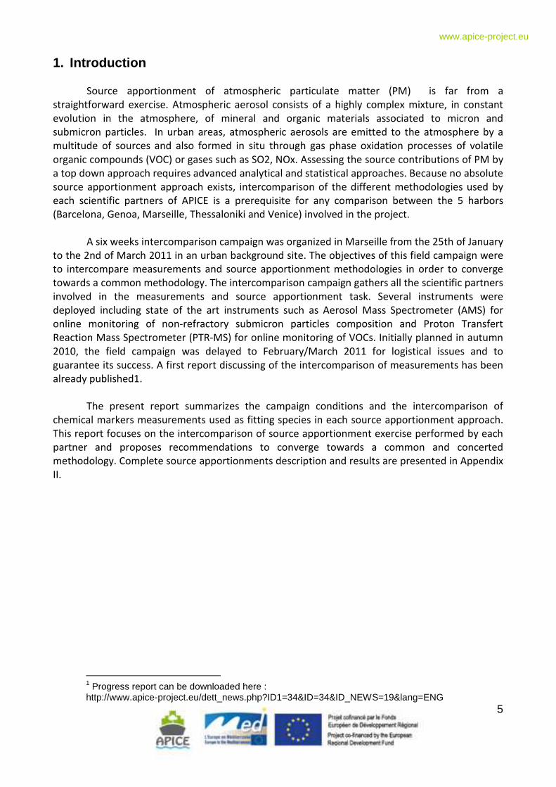
2.1. Sampling site and measurements The intercomparison campaign took place at Marseilles from the 25th of January to the

2nd of March 2011. The sampling site, called « 5 avenues » (43°18’20’’ N, 5°23’40’’ E, 64 m a.s.l. –

figure 2.1), was located in a urban background environment in a large landscape park.

Figure 2.1 : Sampling site localisation and instrumentation deployed during the APICE intercomparison

campaign

The measurement campaign gathered all of the APICE scientific partners on the same

sampling site. A large set of instruments was deployed during the whole campaign allowing the

constant monitoring of aerosol physico-chemical parameters and associated gas phase (VOC’s and

regulated pollutants –ie: O3, NOx, SO2-) (table 2-1). This instrumentation includes all samplers and

analyzers to be used by each scientific partner of APICE as part of the long monitoring campaign

carried out in each harbor. State of the art instrumentations (AMS, PTRMS) and 14

C analyses have

been added to the APICE instrumental setup in order to better constrain the source receptor

models outputs.

2 Progress report can be downloaded here : http://www.apice-project.eu/dett_news.php?ID1=34&ID=34&ID_NEWS=19&lang=ENG

7

ww

w.a

pice

-pro

ject

.eu

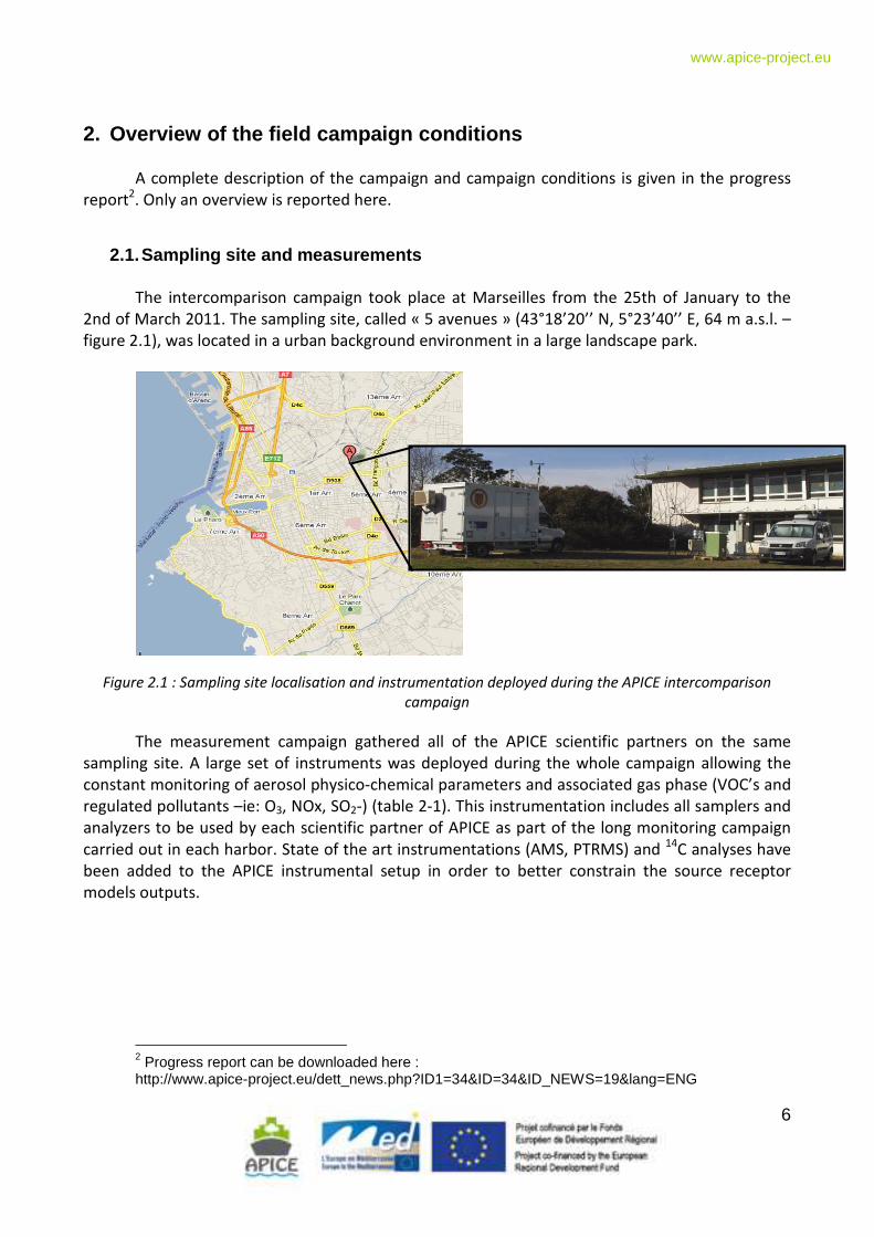
Parameters PMx Time resolution Organization/Lab Instrument/method

MarseilleOrg, SO4, NO3, NH4, (PAH), NR_Cl PM1 7 min LCP-IRA (Univ Prov) HR-ToF-AMSBC PM1 5 min LCP-IRA (Univ Prov) MAAP5012particle number, size distr. PM1 7 min LCP-IRA (Univ Prov) SMPS (10-1000 nm)VOC's (Benz, Tol, isopr, MACR/MVK etc..) 1 min LCP-IRA (Univ Prov) HS-PTRMSOC/EC, majors ions, metals PM2.5 24h LCP-IRA (Univ Prov) Off line HV, OC:EC (EUSAAR2), ions IC, Metals (ICP/MS)Organic markers (levoglucosan, hopanes, n-alk, sterols, PAH, ..) PM2.5 24h LCP-IRA (Univ Prov) Off line HV, GC/MS 14C PM2.5 24h LCP-IRA (Univ- Off line HV Wind dir. and speed, HR, T 5 min LCP-IRA (Univ Prov)SO2, O3, NOx, PM10, PM10 FDMS, PM2.5 FDMS 15 min AtmoPACA PM by TEOM

Source apportionment by CMBThessalonikiOC/EC, majors ions, metals PM2.5 24h ETL/UOWM Off line LV OC:EC (Sunset), ions IC, Metals (ICP/MS or AES)Organic markers ( PAH) PM2.5 24h ETL/UOWM Off line LV, GC/MS PM concentration PM2.5 24h ETL/UOWM Off line LV, Gravimetric

Source apportionment by PMFVeniceSPAH (total Surface Polycyclic Aromatic Hydrocarbons) PM1 5 min ARPAV-ORAR Photoelectric Aerosol Sensor PAS2000 EcoChem (10-1000 nm)PM mass PM2.5 5 min ARPAV-ORAR PM2.5 continuous particle sizing monitor / Dual Wavelength NephelometerPM particle diameter of mass max concentration PM2.5 5 min ARPAV-ORAR PM2.5 continuous particle sizing monitor / Dual Wavelength NephelometerParticle number PM 0.3-10.0 15 min ARPAV-ORAR Handheld 3016IAQ six classes OPC ( 0.3, 0.5, 1.0, 2.5, 5.0, 10.0)Organic markers ( hopanes, n-alkanes, PAH) PM2.5 24h ARPAV-ORAR Off line LV, DTD-GC-MS PM2.5 PM2.5 24h ARPAV-ORAR PM by TECORA gravimetric

Source apportionment by PMFGenoa

PM2.5 PM2.5 12 hDept. of Physics Genoa

sequential sampling on 47 mm quartz and/or teflon filter (porosity 2 micron). Gravimetric, XRF, EC/OC analysis, maybe ions

Particle number concentration in 31 size bins between 0.25 and 18 PM10 1 h Dept. of Physics Grimm Optical Particle CounterBC concentration by optical attenuation measurement PM10 20 m Dept. of Physics Two-wavelength Aethalometer

Source apportionment by PMFBarcelona

Major and trace elements, OC, EC, SO42-, NO3-, Cl- and NH4+ PM10, PM2.5 24h IDAEA-CSICHigh-vol, quartz filters. ICP-AES, ICP-MS, SUNSET (eusaar_2), IC, Electrode for ammonium

PM mass concentration PM10,2.5,1 1h IDAEA-CSIC GRIMM optical counterSource apportionment by PMF

Extern. PartnersTrace elements, metals PM10, PM2.5, PM1 2 h PSI/LAC RDI (Rotating Drum Impactor), with synchrotron-radiation induced X-ray

fluorescenceBC TSP 5 min LA/CNRS Aethalometer 7 lambda

T

ab

le 2

.1 O

verv

iew

of

the

inst

rum

en

tati

on

s d

ep

loye

d d

uri

ng

th

e i

nte

rco

mp

ari

son

ca

mp

aig

n

8


2.2. Field campaign conditions

more than 3 m.s-1

2.5 to 3 m.s-1

2 to 2.5 m.s-1

1.5 to 2 m.s-1

1 to 1.5 m.s-1

0.5 to 1 m.s-1

0 to 0.5 m.s-1

Legend :

more than 3 m.s-1

2.5 to 3 m.s-1

2 to 2.5 m.s-1

1.5 to 2 m.s-1

1 to 1.5 m.s-1

0.5 to 1 m.s-1

0 to 0.5 m.s-1

Legend :

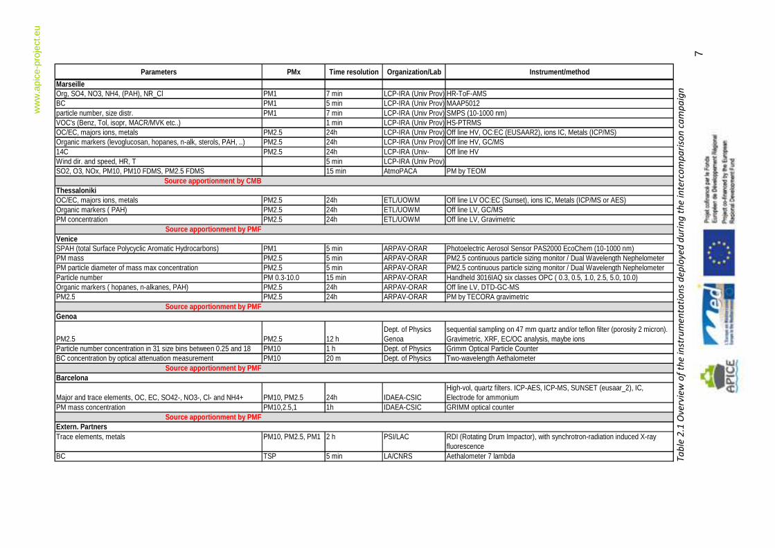
Figure 2.2: Wind direction observed during the intercomparison campaign

Figure 2.2 presents the main local wind directions observed during the measurement

campaign. Three wind directions prevailed: north western winds (Mistral), synoptic south eastern

winds and eastern winds mainly related to nocturnal land breezes. Western winds have also been

observed. Within the framework of APICE north western and western winds are the most

important because in those situations the sampling site is downwind the harbors and industrial

area. Air quality observed during the field campaign was typical for the season in Marseille (38

µg m-3

for PM10; 25 µg m-3

for PM2.5 and 17 µg m-3

for PM1). However these average values hide

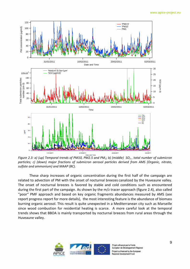
an important variability with periods characterized by high concentrations. Figure 2.3 present the

temporal trends of PM10, PM2.5 and PM1 mass concentrations, SO2, total number concentration

of submicron aerosol particles and of the major chemical fractions of PM1. Fine particles are

dominated by organics (representing 55% of the PM1) followed by nitrate (20%) and BC (9%).

Sulfate and ammonium contribute only to 7 and 8% of the PM1, respectively. Then the total

carbonaceous fraction (Org + BC) represents approximately 2/3 of the total PM1 mass. This result

is not totally surprising in winter, but such a contribution of organic materials indicates a strong

influence of combustion sources (oil derivatives and biomass combustions). It is interesting to

note that the prevalence of the carbonaceous fraction is particularly marked during the first part

of the campaign where sharp increases of their concentration are observed.

9


120

100

80

60

40

20

0

PM

con

cent

ratio

n (µ

g/m

3)

31/01/2011 10/02/2011 20/02/2011 02/03/2011Date and Time

'PM2.5' 'PM10' PM1

120x103

100

80

60

40

20

cm-3

31/01/2011 10/02/2011 20/02/2011 02/03/2011Time

30

25

20

15

10

5

0

SO

2 (µ

g.m

-3)

'Ntot(cm-3) Dp<1µm' 'SO2 (µg/m3)'

Tot

al s

ubm

icro

npa

rtic

les

num

ber

(cm

-3)

Figure 2.3: a) (up) Temporal trends of PM10, PM2.5 and PM1; b) (middle) SO2 , total number of submicron

particles; c) (down) major fractions of submicron aerosol particles derived from AMS (Organic, nitrate,

sulfate and ammonium) and MAAP (BC).

These sharp increases of organic concentration during the first half of the campaign are

related to advection of PM with the onset of nocturnal breezes canalized by the Huveaune valley.

The onset of nocturnal breezes is favored by stable and cold conditions such as encountered

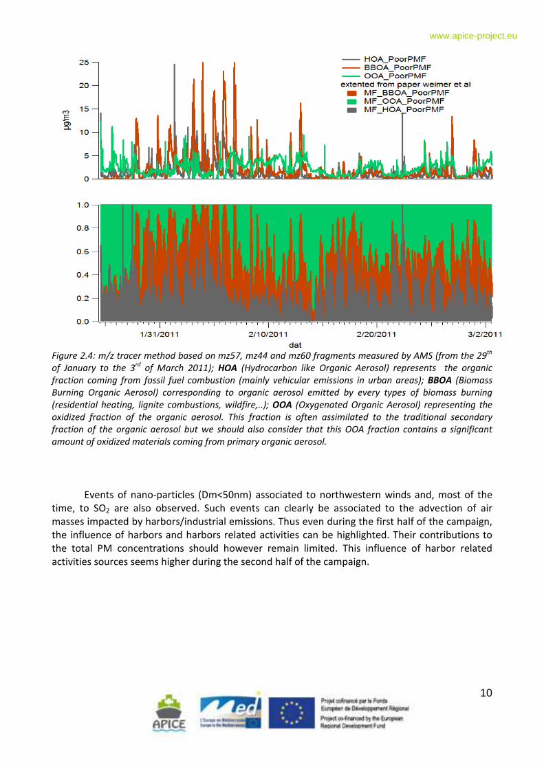
during the first part of the campaign. As shown by the m/z tracer approach (figure 2.4), also called

“poor“ PMF approach and based on key organic fragments abundances measured by AMS (see

report progress report for more details), the most interesting feature is the abundance of biomass

burning organic aerosol. This result is quite unexpected in a Mediterranean city such as Marseille

since wood combustion for residential heating is scarce. A more careful look at the temporal

trends shows that BBOA is mainly transported by nocturnal breezes from rural areas through the

Huveaune valley.

10


Figure 2.4: m/z tracer method based on mz57, mz44 and mz60 fragments measured by AMS (from the 29

th

of January to the 3rd

of March 2011); HOA (Hydrocarbon like Organic Aerosol) represents the organic

fraction coming from fossil fuel combustion (mainly vehicular emissions in urban areas); BBOA (Biomass

Burning Organic Aerosol) corresponding to organic aerosol emitted by every types of biomass burning

(residential heating, lignite combustions, wildfire,..); OOA (Oxygenated Organic Aerosol) representing the

oxidized fraction of the organic aerosol. This fraction is often assimilated to the traditional secondary

fraction of the organic aerosol but we should also consider that this OOA fraction contains a significant

amount of oxidized materials coming from primary organic aerosol.

Events of nano-particles (Dm<50nm) associated to northwestern winds and, most of the

time, to SO2 are also observed. Such events can clearly be associated to the advection of air

masses impacted by harbors/industrial emissions. Thus even during the first half of the campaign,

the influence of harbors and harbors related activities can be highlighted. Their contributions to

the total PM concentrations should however remain limited. This influence of harbor related

activities sources seems higher during the second half of the campaign.

11


3. Summary of the intercomparison of measurements

During the intercomparison campaign in Marseille each scientific partner participated by

using its instrumentation and analytical techniques. In some cases, certain chemical species were

determined only by one of the partners, whereas a number of chemical components were

analyzed in all the laboratories. In this report we show the intercomparison of those species

determined in most of the laboratories (Table 3.1). Please note that UOWM, Univ Provence and

ARPAV also analysed organic markers. Results are presented in appendix I.

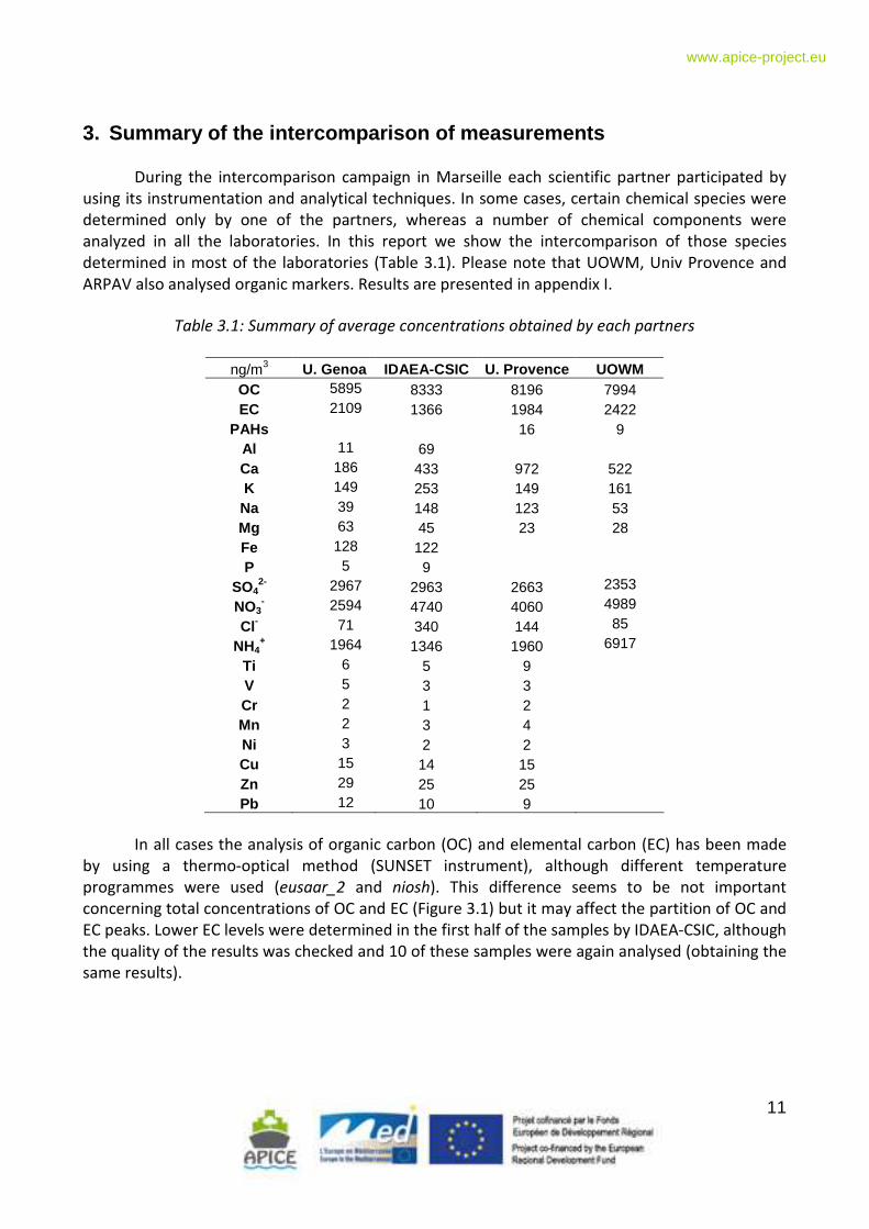
Table 3.1: Summary of average concentrations obtained by each partners

ng/m3 U. Genoa IDAEA-CSIC U. Provence UOWM OC 5895 8333 8196 7994 EC 2109 1366 1984 2422

PAHs 16 9 Al 11 69 Ca 186 433 972 522 K 149 253 149 161 Na 39 148 123 53 Mg 63 45 23 28 Fe 128 122 P 5 9

SO42- 2967 2963 2663 2353

NO3- 2594 4740 4060 4989

Cl- 71 340 144 85

NH4+ 1964 1346 1960 6917

Ti 6 5 9 V 5 3 3 Cr 2 1 2 Mn 2 3 4 Ni 3 2 2 Cu 15 14 15 Zn 29 25 25 Pb 12 10 9

In all cases the analysis of organic carbon (OC) and elemental carbon (EC) has been made

by using a thermo-optical method (SUNSET instrument), although different temperature

programmes were used (eusaar_2 and niosh). This difference seems to be not important

concerning total concentrations of OC and EC (Figure 3.1) but it may affect the partition of OC and

EC peaks. Lower EC levels were determined in the first half of the samples by IDAEA-CSIC, although

the quality of the results was checked and 10 of these samples were again analysed (obtaining the

same results).

12


0

5

10

15

20

25

22-1 27-1 1-2 6-2 11-2 16-2 21-2 26-2 3-3

OC

(µ

g/

m3

)

UOWM CSIC PROV GENOA

0

1

2

3

4

5

6

22-1 27-1 1-2 6-2 11-2 16-2 21-2 26-2 3-3

EC

(µ

g/

m3

)


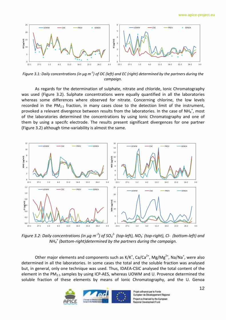
Figure 3.1: Daily concentrations (in µg m

-3) of OC (left) and EC (right) determined by the partners during the

campaign.

As regards for the determination of sulphate, nitrate and chloride, Ionic Chromatography

was used (Figure 3.2). Sulphate concentrations were equally quantified in all the laboratories

whereas some differences where observed for nitrate. Concerning chlorine, the low levels

recorded in the PM2.5 fraction, in many cases close to the detection limit of the instrument,

provoked a relevant divergence between results from the laboratories. In the case of NH4+, most

of the laboratories determined the concentrations by using Ionic Chromatography and one of

them by using a specifc electrode. The results present significant divergences for one partner

(Figure 3.2) although time-variability is almost the same.

0

2

4

6

8

10

12

22-1 27-1 1-2 6-2 11-2 16-2 21-2 26-2 3-3

SO4

2-

(µg/

m3

)


0

2

4

6

8

10

12

14

16

22-1 27-1 1-2 6-2 11-2 16-2 21-2 26-2 3-3

NO

3-

(µg

/m

3)


0,0

0,2

0,4

0,6

0,8

1,0

1,2

22-1 27-1 1-2 6-2 11-2 16-2 21-2 26-2 3-3

Cl-

(µg

/m

3)


0

5

10

15

20

25

22-1 27-1 1-2 6-2 11-2 16-2 21-2 26-2 3-3

NH

4+

(µ

g/

m3

)


Figure 3.2: Daily concentrations (in µg m

-3) of SO4

2- (top-left), NO3

- (top-right), Cl- (bottom-left) and

NH4+ (bottom-right)determined by the partners during the campaign.

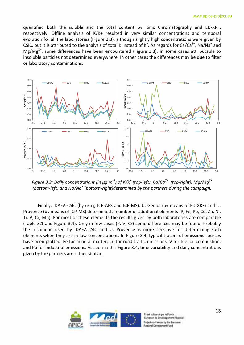
Other major elements and components such as K/K

+, Ca/Ca

2+, Mg/Mg

2+, Na/Na

+, were also

determined in all the laboratories. In some cases the total and the soluble fraction was analysed

but, in general, only one technique was used. Thus, IDAEA-CSIC analysed the total content of the

element in the PM2.5 samples by using ICP-AES, whereas UOWM and U. Provence determined the

soluble fraction of these elements by means of Ionic Chromatography, and the U. Genoa

13


quantified both the soluble and the total content by Ionic Chromatography and ED-XRF,

respectively. Offline analysis of K/K+ resulted in very similar concentrations and temporal

evolution for all the laboratories (Figure 3.3), although slightly high concentrations were given by

CSIC, but it is attributed to the analysis of total K instead of K+. As regards for Ca/Ca

2+, Na/Na

+ and

Mg/Mg2+

, some differences have been encountered (Figure 3.3), in some cases attributable to

insoluble particles not determined everywhere. In other cases the differences may be due to filter

or laboratory contaminations.

0,00

0,10

0,20

0,30

0,40

0,50

0,60

0,70

22-1 27-1 1-2 6-2 11-2 16-2 21-2 26-2 3-3

K/

K+

(µ

g/

m3

)


0,00

0,50

1,00

1,50

2,00

2,50

3,00

3,50

22-1 27-1 1-2 6-2 11-2 16-2 21-2 26-2 3-3C

a/

Ca

2+

(µ

g/

m3

)


0,00

0,05

0,10

0,15

0,20

22-1 27-1 1-2 6-2 11-2 16-2 21-2 26-2 3-3

Mg

/M

g2

+ (

µg

/m

3)


0,00

0,10

0,20

0,30

0,40

0,50

22-1 27-1 1-2 6-2 11-2 16-2 21-2 26-2 3-3

Na

/N

a+

(µ

g/

m3

)


Figure 3.3: Daily concentrations (in µg m-3

) of K/K+ (top-left), Ca/Ca

2+ (top-right), Mg/Mg

2+

(bottom-left) and Na/Na+ (bottom-right)determined by the partners during the campaign.

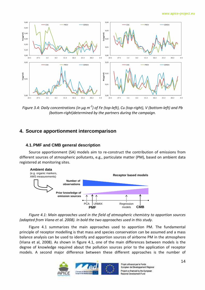
Finally, IDAEA-CSIC (by using ICP-AES and ICP-MS), U. Genoa (by means of ED-XRF) and U.

Provence (by means of ICP-MS) determined a number of additional elements (P, Fe, Pb, Cu, Zn, Ni,

Ti, V, Cr, Mn). For most of these elements the results given by both laboratories are comparable

(Table 3.1 and Figure 3.4). Only in few cases (P, V, Cr) some differences may be found. Probably

the technique used by IDAEA-CSIC and U. Provence is more sensitive for determining such

elements when they are in low concentrations. In Figure 3.4, typical tracers of emissions sources

have been plotted: Fe for mineral matter; Cu for road traffic emissions; V for fuel oil combustion;

and Pb for industrial emissions. As seen in this Figure 3.4, time variability and daily concentrations

given by the partners are rather similar.

14


0,00

0,10

0,20

0,30

0,40

0,50

0,60

22-1 27-1 1-2 6-2 11-2 16-2 21-2 26-2 3-3

Fe

(µ

g/

m3

)

CSIC PROV GENOA

0,00

0,01

0,02

0,03

0,04

22-1 27-1 1-2 6-2 11-2 16-2 21-2 26-2 3-3

Cu

(µ

g/

m3

)

CSIC PROV GENOA

0,00

0,01

0,02

22-1 27-1 1-2 6-2 11-2 16-2 21-2 26-2 3-3

V (

µg

/m

3)

CSIC PROV GENOA

0,00

0,01

0,02

0,03

22-1 27-1 1-2 6-2 11-2 16-2 21-2 26-2 3-3

Pb

(µ

g/

m3

)

CSIC PROV GENOA

Figure 3.4: Daily concentrations (in µg m-3

) of Fe (top-left), Cu (top-right), V (bottom-left) and Pb

(bottom-right)determined by the partners during the campaign.

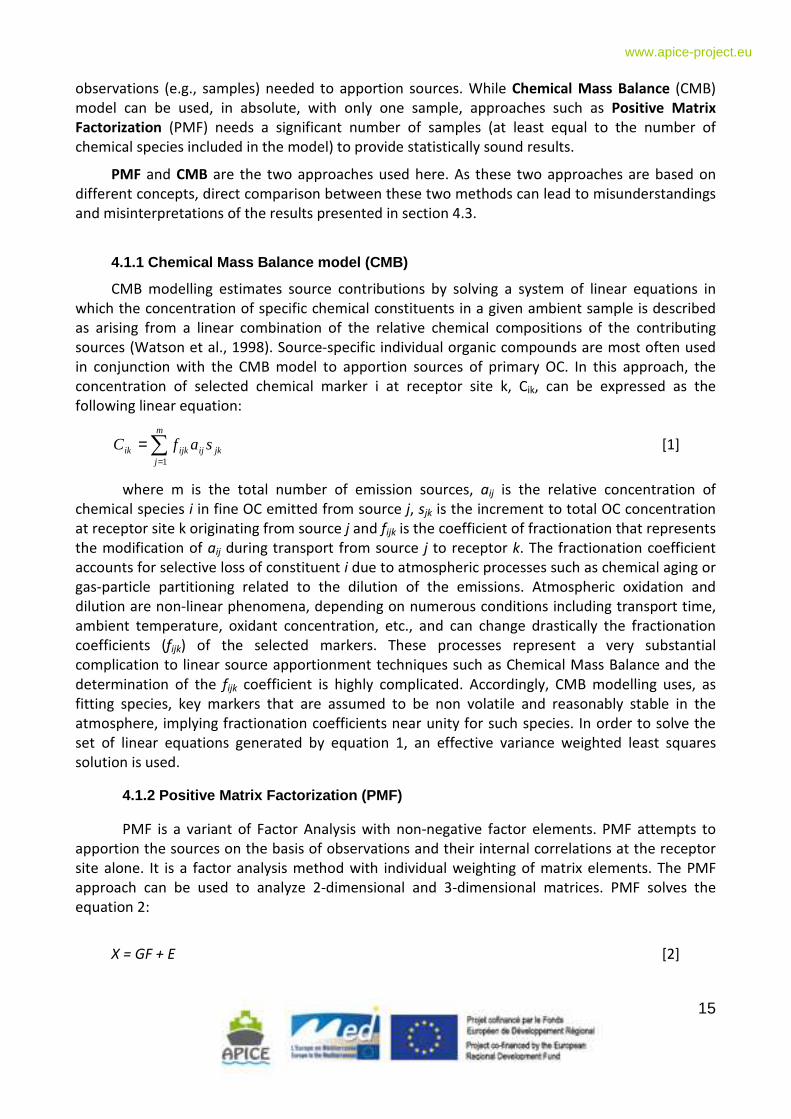
4. Source apportionment intercomparison

4.1. PMF and CMB general description

Source apportionment (SA) models aim to re-construct the contribution of emissions from

different sources of atmospheric pollutants, e.g., particulate matter (PM), based on ambient data

registered at monitoring sites.

PMF CMB

Prior knowledge of emission sources

Number of observations

Receptor based models

Ambient data(e.g. organic markers, AMS measurements)

PCA UNMIX Regressionmodels

Figure 4.1: Main approaches used in the field of atmospheric chemistry to apportion sources

(adapted from Viana et al. 2008). In bold the two approaches used in this study.

Figure 4.1 summarizes the main approaches used to apportion PM. The fundamental

principle of receptor modelling is that mass and species conservation can be assumed and a mass

balance analysis can be used to identify and apportion sources of airborne PM in the atmosphere

(Viana et al, 2008). As shown in figure 4.1, one of the main differences between models is the

degree of knowledge required about the pollution sources prior to the application of receptor

models. A second major difference between these different approaches is the number of

15


observations (e.g., samples) needed to apportion sources. While Chemical Mass Balance (CMB)

model can be used, in absolute, with only one sample, approaches such as Positive Matrix

Factorization (PMF) needs a significant number of samples (at least equal to the number of

chemical species included in the model) to provide statistically sound results.

PMF and CMB are the two approaches used here. As these two approaches are based on

different concepts, direct comparison between these two methods can lead to misunderstandings

and misinterpretations of the results presented in section 4.3.

4.1.1 Chemical Mass Balance model (CMB)

CMB modelling estimates source contributions by solving a system of linear equations in

which the concentration of specific chemical constituents in a given ambient sample is described

as arising from a linear combination of the relative chemical compositions of the contributing

sources (Watson et al., 1998). Source-specific individual organic compounds are most often used

in conjunction with the CMB model to apportion sources of primary OC. In this approach, the

concentration of selected chemical marker i at receptor site k, Cik, can be expressed as the

following linear equation:

∑=

=m

jjkijijkik safC

1

[1]

where m is the total number of emission sources, aij is the relative concentration of

chemical species i in fine OC emitted from source j, sjk is the increment to total OC concentration

at receptor site k originating from source j and fijk is the coefficient of fractionation that represents

the modification of aij during transport from source j to receptor k. The fractionation coefficient

accounts for selective loss of constituent i due to atmospheric processes such as chemical aging or

gas-particle partitioning related to the dilution of the emissions. Atmospheric oxidation and

dilution are non-linear phenomena, depending on numerous conditions including transport time,

ambient temperature, oxidant concentration, etc., and can change drastically the fractionation

coefficients (fijk) of the selected markers. These processes represent a very substantial

complication to linear source apportionment techniques such as Chemical Mass Balance and the

determination of the fijk coefficient is highly complicated. Accordingly, CMB modelling uses, as

fitting species, key markers that are assumed to be non volatile and reasonably stable in the

atmosphere, implying fractionation coefficients near unity for such species. In order to solve the

set of linear equations generated by equation 1, an effective variance weighted least squares

solution is used. 4.1.2 Positive Matrix Factorization (PMF) PMF is a variant of Factor Analysis with non-negative factor elements. PMF attempts to

apportion the sources on the basis of observations and their internal correlations at the receptor

site alone. It is a factor analysis method with individual weighting of matrix elements. The PMF

approach can be used to analyze 2-dimensional and 3-dimensional matrices. PMF solves the

equation 2:

X = GF + E [2]

16


where X is the matrix of measured values (time series of the different fitting species), G and

F are the factor matrices to be determined, and E is the matrix of residuals, the unexplained part

of X. F and G represent respectively the contribution of each fitting species to a factor (e.g., source

and/or processes) and the time series of the contribution of the different factors. In PMF, the

solution is a weighted Least Squares fit, where the known standard deviations for each value of X

are used for determining the weights of the residuals in matrix E. The objective of PMF is to

minimize the sum of the weighted residuals. PMF uses information from all samples by weighting

the squares of the residuals with the reciprocals of the squares of the standard deviations of the

data values. 4.1.3 Summary CMB model is based on the mass conservation of individual species and carbon from

sources to the receptor sites. The mass conservation equations are written as the matrix product

of unknown time series of source contributions and known source profiles equaling the time series

of known concentrations of a set of marker species observed. Therefore the CMB model assumes

knowledge of the chemical fingerprints of the emissions for all relevant sources. This last point is

most of the time a critical issue. As CMB model apportion primary sources, the secondary fraction

can not be apportioned directly. Secondary fraction of sulfate, nitrate, ammonium and organic

aerosol can only be assessed by difference between measured (primary + secondary fractions) and

calculated concentrations (primary fraction).

For PMF, the mass conservation equations are written as a matrix product of unknown

time series of factor (e.g., sources and/or processes) contributions and unknown factors (to be

determined and identified) equaling the times series of known concentrations of a set of marker

species observed. The most difficult challenge in using PMF is determining the number of factor (ie

sources) that are contributing to the PM collected at the receptor site and to identify these

factors. The degrees of freedom in the PMF approach are contained inside the different factors

and more precisely in the relative contribution of the different fitting species in each factor.

4.2. Methodology used by each partners The aim of this intercomparison of source apportionment approaches was to keep totally

free each partner to choose their own approach and fitting species. Source apportionment results

obtained by the different partners of the project are fully described and commented in appendix

II. A short description is given below.

4.2.1. Barcelona (IDAEA-CSIC) The identification of the main PM sources and their contribution to PM10 and PM2.5 during

the intercomparison campaign in Marseille was carried out by a source apportionment analysis

with Positive Matrix Factorization (PMF; Paatero and Tapper, 1994), through the computer

program PMF2 (Paatero, 1997).

The PMF analysis was performed on 74 cases, including simultaneous daily PM10 and PM2.5

filter samples, collected from 25/01/2011 to 01/03/2011.

17


Chemical species were selected according to Signal to Noise ratios (Paatero and Hopke,

2003), to the percentage of values above detection limits and to the database size requirements.

For this analysis 22 species analyzed from the filter samples were selected, including Ca, K, Na, Mg,

Fe, Mn, SO42-

(from ICP-AES); V, Ni, Cu, Zn, Sn, Sb, Pb (ICP-MS); NO3- (ion chromatography); NH4

+

(ion selective electrode), and EC and five OC fractions (OC1, OC2, OC3, OC4 and Pyrolitic C)

provided by the Sunset OCEC thermo-optical analyzer (EUSAAR2 protocol, Cavalli et al., 2010).

Individual uncertainties were calculated following the procedure described by Amato et al.

(2009) and Escrig et al. (2009), taking into account the analytical uncertainty as well as the

standard deviations of species concentrations in the blank filters.

Emission sources were identified by taking into account the PMF-resolved chemical profile

and the variation explained by each factor for every species. Daily contributions of each source to

PM10 and PM2.5 were calculated by a multilinear regression analysis.

4.2.2. Genoa (Univ Genoa) The source apportionment approach used by Genoa’s group is PMF2 (Positive Matrix

Factorization, version 2), an advanced receptor model, developed by Paatero (Paatero et al, 1994)

that in the last years has been asserted to international level like most reliable. It is useful,

especially, where detailed data do not exist on the composition of the main emission sources, but

where large numbers of sampled data are available on ambient concentrations. The important

advantage of the positive matrix factorization is the ability to handle missing data and values

below the detection limits data by adjusting the error estimates of each data point. In fact, the

solution to the PMF problem depends on the uncertainties attributed to each value. The

concentrations values and their associated errors were treated according to Polissar et al. (Polissar

et al, 1998). PMF was used in “robust mode”.

For this approach, PM measured components used for PMF analysis included elements

measures by ED-XRF, ions detected by ion chromatography (IC) and organic and elemental carbon

measured by thermal-optical transmittance method (TOT). In the PMF data set, OC missing values

were replaced using the mean OC/EC ratio with a large uncertainty. Variables were selected

according to the signal-to-noise criterion (Paatero and Hopke, 2002) and 15 Variables were finally

used in the analysis: Al, Si, P, K, Ca, V, Fe, Ni, Cu, Zn, SO42-

, NH4+, NO3

-, OC and EC. Na and Cl turned

out to be “bad” variables (are present in a low number of samples because of PM2.5 sampling

were performed and Na values are available each two days). This prevented the possibility to

resolve PM from sea salt.

The number of factors which was examined ranged from three to eight; five sources

were resolved and labeled, according to their characteristic tracers, as follows: Road (traced by

Cu), Dust (traced by Al, Si, Ca), Industrial/Marin (Oil Combustion traced by V, Ni), Secondary

Compound (Secondary I traced by SO42-

and NH4+

and Secondary II traced by NO3- and NH4

+).

4.2.3. Marseille (Aix Marseille Univ.) The CMB source apportionment was computed using United States Environmental

Protection agency EPA-CMB8.2 software, in conjunction with the effective variance least squares

estimation method.

18


The source emission profiles selected for this study were : vehicular emissions, (El Haddad

et al., 2009) ; heavy duty trucks emissions (Rogge et al., 1993a) ; biomass burning emissions (Fine

et al., 2002) ; vegetative detritus emissions (Rogge et al., 1993b), and natural gas combustion

(Rogge et al., 1993b). Considering the specific case of Marseille area, three industrial-emission-

related profiles were also selected: metallurgical coke production (Weitkamp et al., 2005), HFO

combustion/shipping (Agrawal et al., 2008) and steel manufacturing (Tsai et al., 2007).

In order to assess contributions from these aforementioned sources, were used as fitting

species: levoglucosan, specific marker for biomass burning ; elemental carbon (EC) and three

hopanes (i.e., 17α(H),21β(H)-norhopane, 17α(H),21β(H)-hopane and 22S,17α(H),21β(H)-

homohopane) as key markers for vehicular emissions ; C27-C32 n-alkanes, since this range

demonstrates high odd-carbon preference that is specific to biogenic sources ; and four PAH

(benzo[b,k]fluoranthene, benzo[e]pyrene, indeno[1,2,3-cd]pyrene, and benzo[ghi]perylene) and

three metals (V, Ni and Pb), to apportion for industrial sources.

To insure a good quality control of CMB calculation results, we make sure that the

statistical performance measures usually used in the CMB modeling meet their respective target

values (i.e. R-square from 0.8 to 1.0, chi-square from 0 to 4.0, t-test above 2 and absence of

cluster sources). Another requirement was for the marker’s calculated-to-measured ratios (C/M)

to match a target value fixed between 0.75 and 1.25, in order to provide reasonable bounds on

CMB results.

As CMB can not apportion directly Sea salt and dust contributions, empirical approaches

have been used for these two sources. Crustal dust contributions were then estimated using Malm

et al. (1994) method based on concentrations of Al, Fe, Ca and Ti in PM samples. Sea salt were

calculated according to Putaud et al. (2010) method, based on Cl- and Na

+ concentrations in PM

samples.

4.2.4. Thessaloniki (UOWM)

For the source apportionment analysis conducted from UOWM, Positive Matrix Factorization

model (version 3.0) was used. The analysis was performed on 37 PM2.5 samples (provided by

CSIC-IDAEA). From the available chemical analysis data, selected species were injected to the

model:

• 8 selected PAHs: Benzo[b]fluoranthene, Benzo[k]fluoranthene, Benzo[e]pyrene,

Benzo[a]pyrene, Perylene, Indeno[cd]pyrene, Dibenzo[a,h]anthracene, Benzo[ghi]perylene.

Lighter PAHs were excluded from the analysis because of their volatility.

• 3 selected ions: NO3-, SO4

2-, NH4

+.

• 23 metals: Al, Ca, K, Na, Mg, Fe, Mn, Ti, P, V, Cr, Ni, Cu, Zn, As, Rb, Sr, Sb, Cd, Sn, Pb, Li, Sb,

La.

• Organic and elemental carbon (OC, EC)

Data pre-treatment and analysis of input data included missing data and data below the

detection limit replacement. Species with large analytical errors were excluded from the analysis.

Species which presented low signal-to-noise ratio were characterized as "weak". The model was

run for 3 to 10 factors, in a random seed and the optimal number of factors was six. Finally,

bootstrap and Fpeak runs were conducted in order to examine the stability and the rotational

ambiguity of the solution, respectively.

19


4.2.5. Venice (Arpav Veneto) IDAEA group performed the source apportionment analysis also on the organic species

measured by ARPAV. The source apportionment approach used by IDAEA group is PMF2 (Positive

Matrix Factorization, version 2), an advanced receptor model, developed by Paatero (Paatero et

al, 1994) that in the last years has been asserted to international level like most reliable. It is

useful, especially, where detailed data do not exist on the composition of the main emission

sources, but where large numbers of sampled data are available on ambient concentrations. The

important advantage of the positive matrix factorization is the ability to handle missing data and

values below the detection limits data by adjusting the error estimates of each data point. In fact,

the solution to the PMF problem depends on the uncertainties attributed to each value. The errors

associated to concentrations values were treated according to the procedure described by Amato

et al. (2009) and Escrig et al. (2009).

In the presented PMF analysis, PM measured components included elements, ions, organic

and elemental carbon measured by IDAEA group and targeted sum of the organic species

described in Appendix 1: Even Alkanes (E-ALK: n-C(26-28-30-32)), Odd Alkanes (O-ALK: n-C(27-29-

31-33)), Heavy PAH (H-PAH: Benzo(b)fluoranthene, Benzo(j+k)fluoranthene, Benzo(a)pyrene,

Indeno(123-cd)pyrene, Dibenz(a,h)anthracene, Benzo(ghi)perylene), Hopanes (HOPA: 17alpha(H)-

22,29,30-Trisnorhopane, 17alpha(H),21beta(H)-30-Norhopane, 17alpha(H),21beta(H)-Hopane,

17alpha(H),21beta(H)-22S-Homohopane, 17alpha(H),21beta(H)-22R-Homohopane) and DeHydro

Abietic Acid (DHAA) measured by ARPAV.

Variables were selected according to the signal-to-noise criterion (Paatero and Hopke,

2003) and 21 Variables were finally used in the analysis: Ca, Na, Mg, Fe, SO42-

, V, Ni, Cu, Zn, Sn,

Sb, Pb, NO3-, NH4

+, EC, OC, E-ALK, O-ALK, H-PAH, HOPA, DHAA.

Seven sources were resolved and labeled, according to their characteristic tracers, as follows: Dust

(traced by Ca), Road (divided into Vehicular exhaust + Sea Spray (traced by Cu, Zn, EC and Na) and

Road Dust (traced by Sb and Sn), Industrial/Marine (Oil Combustion, traced by V, Ni), Secondary

Compound divided into Secondary I (traced by SO42-

) and Secondary II (traced by NO3-) and

Residential (Biomass Burning, traced by DHAA).

4.3. Intercomparison of source apportionment approa ches

As described section 4.2 and in appendix II, many sources or source types have been

identified and quantified. Some of them can directly be compared some of them not directly. In

order to intercompare the results of source contributions or source types have been classified

onto 5 source groups. This classification has been elaborated in collaboration with modelers in

order to allow a direct comparison of source contributions with models outputs. The 5 source

groups are:

• Road (direct and indirect emissions from traffic),

• residential,

• primary natural,

• Industrial and shipping emissions,

• secondary sources (ie mass of the aerosol formed in the atmosphere from gaseous

precursors).

20


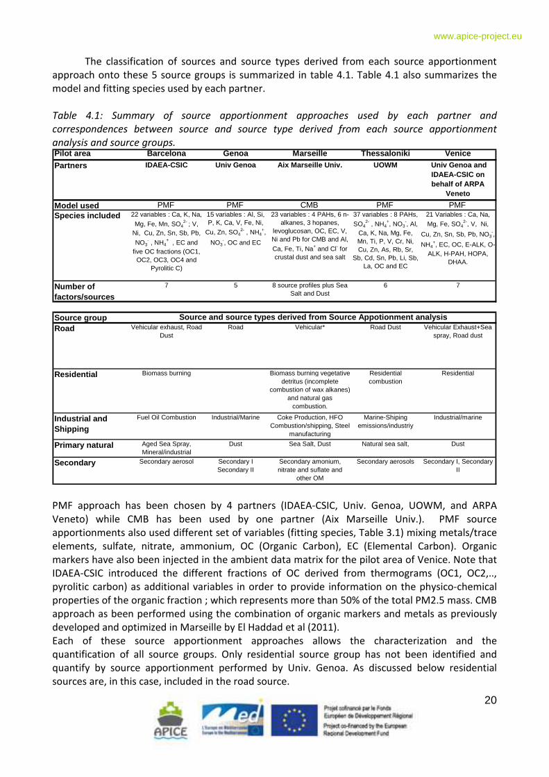
The classification of sources and source types derived from each source apportionment

approach onto these 5 source groups is summarized in table 4.1. Table 4.1 also summarizes the

model and fitting species used by each partner.

Table 4.1: Summary of source apportionment approaches used by each partner and

correspondences between source and source type derived from each source apportionment

analysis and source groups. Pilot area Barcelona Genoa Marseille Thessaloniki Venice

Partners IDAEA-CSIC Univ Genoa Aix Marseille Univ. UOWM Univ Ge noa and IDAEA-CSIC on behalf of ARPA

Veneto

Model used PMF PMF CMB PMF PMFSpecies included 22 variables : Ca, K, Na,

Mg, Fe, Mn, SO42- ; V,

Ni, Cu, Zn, Sn, Sb, Pb,

NO3- , NH4

+ , EC and five OC fractions (OC1,

OC2, OC3, OC4 and Pyrolitic C)

15 variables : Al, Si, P, K, Ca, V, Fe, Ni,

Cu, Zn, SO42- , NH4

+,

NO3-, OC and EC

23 variables : 4 PAHs, 6 n-alkanes, 3 hopanes,

levoglucosan, OC, EC, V, Ni and Pb for CMB and Al,

Ca, Fe, Ti, Na+ and Cl- for crustal dust and sea salt

37 variables : 8 PAHs,

SO42- , NH4

+, NO3-, Al,

Ca, K, Na, Mg, Fe, Mn, Ti, P, V, Cr, Ni, Cu, Zn, As, Rb, Sr,

Sb, Cd, Sn, Pb, Li, Sb, La, OC and EC

21 Variables : Ca, Na,

Mg, Fe, SO42-, V, Ni,

Cu, Zn, Sn, Sb, Pb, NO3-,

NH4+, EC, OC, E-ALK, O-

ALK, H-PAH, HOPA, DHAA.

Number of factors/sources

7 5 8 source profiles plus Sea Salt and Dust

6 7

Source groupRoad Vehicular exhaust, Road

DustRoad Vehicular* Road Dust Vehicular Exhaust+Sea

spray, Road dust

Residential Biomass burning Biomass burning vegetative detritus (incomplete

combustion of wax alkanes) and natural gas

combustion.

Residential combustion

Residential

Industrial and Shipping

Fuel Oil Combustion Industrial/Marine Coke Production, HFO Combustion/shipping, Steel

manufacturing

Marine-Shiping emissions/industriy

Industrial/marine

Primary natural Aged Sea Spray, Mineral/industrial

Dust Sea Salt, Dust Natural sea salt, Dust

Secondary Secondary aerosol Secondary I Secondary II

Secondary amonium, nitrate and suflate and

other OM

Secondary aerosols Secondary I, Secondary II

Source and source types derived from Source Appotio nment analysis

PMF approach has been chosen by 4 partners (IDAEA-CSIC, Univ. Genoa, UOWM, and ARPA

Veneto) while CMB has been used by one partner (Aix Marseille Univ.). PMF source

apportionments also used different set of variables (fitting species, Table 3.1) mixing metals/trace

elements, sulfate, nitrate, ammonium, OC (Organic Carbon), EC (Elemental Carbon). Organic

markers have also been injected in the ambient data matrix for the pilot area of Venice. Note that

IDAEA-CSIC introduced the different fractions of OC derived from thermograms (OC1, OC2,..,

pyrolitic carbon) as additional variables in order to provide information on the physico-chemical

properties of the organic fraction ; which represents more than 50% of the total PM2.5 mass. CMB

approach as been performed using the combination of organic markers and metals as previously

developed and optimized in Marseille by El Haddad et al (2011).

Each of these source apportionment approaches allows the characterization and the

quantification of all source groups. Only residential source group has not been identified and

quantify by source apportionment performed by Univ. Genoa. As discussed below residential

sources are, in this case, included in the road source.

21


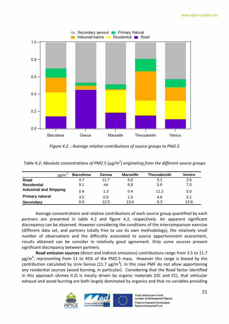
Figure 4.2. : Average relative contributions of source groups to PM2.5

Table 4.2: Absolute concentrations of PM2.5 (µg/m3) originating from the different source groups

µg/m 3 Barcelona Genoa Marseille Thessaloniki VeniceRoad 4.7 11.7 5.0 5.1 3.5Residential 9.1 nd 6.8 5.6 7.0Industrial and Shipping 5.6 1.3 0.4 11.2 5.0Primary natural 3.5 0.9 1.5 4.6 3.1Secondary 9.9 12.0 13.0 6.3 13.8

Average concentrations and relative contributions of each source group quantified by each

partners are presented in table 4.2 and figure 4.2, respectively. An apparent significant

discrepancy can be observed. However considering the conditions of the intercomparison exercise

(different data set, and partners totally free to use its own methodology), the relatively small

number of observations and the difficultly associated to source apportionment assessment,

results obtained can be consider in relatively good agreement. Only some sources present

significant discrepancy between partners.

Road emission sources (direct and indirect emissions) contributions range from 3.5 to 11.7

µg/m3, representing from 11 to 45% of the PM2.5 mass. However this range is biased by the

contribution calculated by Univ Genoa (11.7 µg/m3). In this case PMF do not allow apportioning

any residential sources (wood burning, in particular). Considering that the Road factor identified

in this approach (Annex II.2) is mostly driven by organic materials (OC and EC), that vehicular

exhaust and wood burning are both largely dominated by organics and that no variables providing

22


insights into the chemical nature of this fraction have been injected in this specific source

apportionment exercise, we can consider that the Road factor represents, in fact, the sum of

residential and road sources. This assumption is also supported when comparing the sum of these

2 source groups between all partners. The sum of the contributions of residential and road

sources are very homogeneous between partners, ranging from 10.6 to 13.8 µg/m3.

Residential sources are quasi exclusively related to wood burning sources. The

contributions of other sources such as natural gas combustion or cooking activities are negligible

when they have been identified. The identification of wood burning is unambiguous since this

source is traced by very specific molecular markers (levoglucosan or dehydro abietic acid). A good

agreement is found between partners. Contributions of residential sources range from 5.6 to 9.1

µg/m3. Again a partial overlap between residential and road sources can not be excluded for PMF

approaches using no specific markers for wood burning sources. We shall note that the use of the

different fractions of OC derived from its thermal properties (OC1, OC2,..,pyrolitic C) provide very

promising results to differentiate vehicular emissions from wood burning sources.

Primary natural source group (mainly sea salt and dust) can be regarded as in reasonable

agreement between partners taking into account the different approaches and data set used.

Contribution of primary natural sources ranged from 0.9 to 4.6 µg/m3.

For industrial and secondary factors the situation is a little bit different and these two

factors must be considered together in the discussion. Industrial sources contribution shows a

high discrepancy between partners and approaches ranging from 0.4 to 11.7 µg/m3 (ie from 1 to

34% of PM2.5 mass). If 1% can be consider as low and within the uncertainty range of the method

used (CMB), 34% can not be regarded as a relevant contribution for industrial and shipping

emissions. On the same way, contributions found by IDAEA-CSIC (Barcelona, 17%) and UOWM

(Thessaloniki, 15%) should be considered as overestimated taking into account previous studies

realized in Marseille and its surroundings. The reason of these higher contributions estimated

from the PMF model runs is most probably linked to dynamic processes. As PMF approach is based

on the internal variability of the data set, atmospheric dynamics (advection of air masses or

boundary layer height) can play a major role on the identification and the quantification of the

different factors. Marseille is downwind the industrial area during particular wind conditions:

mistral (NW winds). Mistral is canalized by the Rhône valley (a heavily urbanized and industrial

area), bringing to Marseille in most cases (when moderate winds) high loads of secondary aerosol

particles. Such conditions have been observed during the campaign. Therefore, a significant

fraction of the secondary aerosol particles from medium and long range transport episodes have

been included in the industrial factor by the PMF approach. As for road and residential sources,

this assumption is supported by the fact that the sum of industrial and secondary sources are in

pretty good agreement between partners, ranging from 13.4 to 18.8 µg/m3.

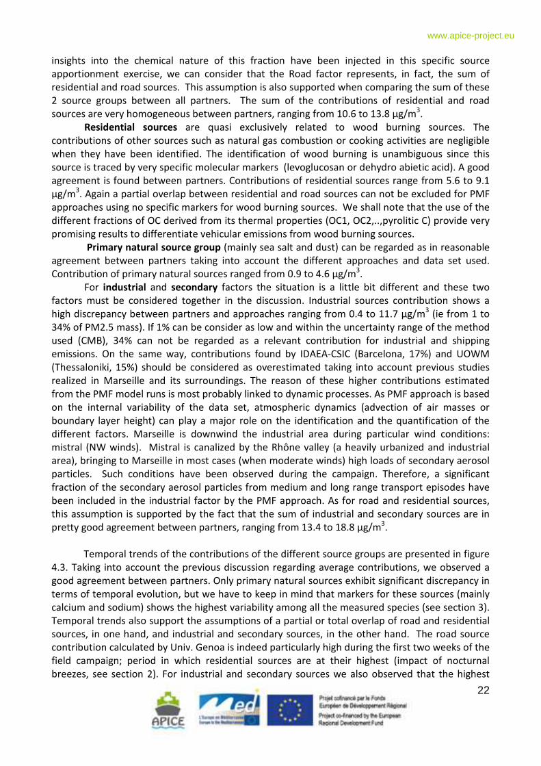
Temporal trends of the contributions of the different source groups are presented in figure

4.3. Taking into account the previous discussion regarding average contributions, we observed a

good agreement between partners. Only primary natural sources exhibit significant discrepancy in

terms of temporal evolution, but we have to keep in mind that markers for these sources (mainly

calcium and sodium) shows the highest variability among all the measured species (see section 3).

Temporal trends also support the assumptions of a partial or total overlap of road and residential

sources, in one hand, and industrial and secondary sources, in the other hand. The road source

contribution calculated by Univ. Genoa is indeed particularly high during the first two weeks of the

field campaign; period in which residential sources are at their highest (impact of nocturnal

breezes, see section 2). For industrial and secondary sources we also observed that the highest

23


contribution of industrial sources correspond to high loadings of secondary aerosol (especially

from 02/05 to 02/15/2011, figure 4.3).

Figure 4.3.: temporal evolution of the contributions (µg/m

3) of the different source groups

quantified.

24


5. Conclusions and perspectives

Within the framework of APICE the aim of the intercomparison campaign was to compare

the source apportionment outputs of each scientific group involved in the long monitoring

campaign carried out in each pilot area. Each partner was totally free to use his own methodology

(measurements and source apportionment model). As expected, significant discrepancies are

observed. However these discrepancies regard mostly the average contribution of some sources

while the temporal trends are in fair agreements. Differences can also be linked quite easily to the

methodology used, either regarding the choice of fitting species or source profiles, either

considering biases induced by the dynamic of the atmosphere (particularly important considering

the number of observations).

In order to converge towards a homogenous methodology between each pilot area, our

recommendations are as follows:

1/ Use of the same source apportionment approach. The source apportionment approach

chosen is PMF (Positive Matrix Factorization). In consequence, Aix Marseille Univ will also use PMF

in addition to CMB,

2/ Use of a common basis of chemical markers as fitting species. The chemical markers list

will include trace elements/metals and organic markers or at least the different carbon fractions

(OC1, OC2,.., Pyrolitic Carbon), in addition to OC, EC, sulfate, nitrate and ammonium. The list of

chemical markers will be defined by the partnership after a careful study of the chemical data

obtained during the long monitoring campaigns. Some additional markers may be added to the list

in each pilot area in order to take into account the specificity of each pilot area,

3/ Common interpretation of the different factors identified in each pilot area.

Currently, a vast intercomparison exercise of source apportionment approaches is

conduced at the European level, in which some partners of the project APICE are associated. The

results obtained within APICE long monitoring campaigns will also directly benefit from this

European intercomparison exercise in terms of methodological harmonization.

25


6. References Agrawal H., Welch W. A., Miller J. W. and Cocker, D. R., 2008. Emission measurements from a crude oil

tanker at sea. Environment Science and Technology 42: 7098-7103.

Aiken A. C., DeCarlo P. F., Kroll J. H., Worsnop D. R., Huffman J. A., Docherty K. S., Ulbrich I. M., Mohr C.,

Kimmel J. R., Sueper D., Sun Y., Zhang Q., Trimborn A., Northway M., Ziemann P. J., Canagaratna M.

R., Onasch T. B., Alfarra M. R., Prevot A. S. H., Dommen J., Duplissy J., Metzger A., Baltensperger U.,

and Jimenez J. L. 2008. O/C and OM/OC Ratios of Primary, Secondary, and Ambient Organic

Aerosols with High-Resolution Time-of-Flight Aerosol Mass Spectrometry. Environment Science and

Technology 42: 4478-4485.

Amato, F., Pandolfi, M., Escrig, A., Querol, X., Alastuey, A., Pey, J., Perez, N., Hopke, P. K., 2009. Quantifying

road dust resuspension in urban environment by multilinear engine: a comparison with PMF2.

Atmospheric Environment 43, 2770-2780.

Birch M.E. and Cary R.A., 1996. Elemental Carbon-basedn method for monitoring occupational exposures to

particulate diesel exhaust. Aerosol Science and Technology 25, 221-241.

Cavalli F., Viana M., Yttri K. E., Genberg J. and Putaud J. P. (2010). Toward a standardised thermal-optical

protocol for measuring atmospheric organic and elemental carbon: the EUSAAR protocol. Atmos.

Meas. Tech., 3, 1, 79-89.

Chow, J.C., Yu, J.Z., Watson, J.G., Hang, S.S., Bohannan, T.L., Hays, M.D., Fung, K.K., 2007. The application of

thermal methods for determining chemical composition of carbonaceous aerosols: A review.

Journal of Environmental Science and Health Part A 42, 1521-1541.

El Haddad I., Marchand N., Dron J., Temime-Roussel B., Quivet E., Wortham H., Jaffrezo J. L., Baduel C.,

Voisin D., Besombes J. L. and Gille, G. 2009. Comprehensive primary particulate organic

characterization of vehicular exhaust emissions in France. Atmospheric Environment 43: 6190-

6198.

El Haddad I., Marchand N., Wortham H., Piot C., BesombesJ.-L., Cozic J., Chauvel C., Armengaud A., Robin D.

and JaffrezoJ.-L. 2011. Primary sources of PM2.5 organic aerosol in an industrial Mediterranean

city, Marseille. Atmospheric Chemistry and Physics 11: 2039-2058,.

Escrig, A., Monfort, E., Celades, I., Querol, X., Amato, F., Minguillon, M.C., Hopke, P., 2009. Application of

optimally scaled target factor analysis for assessing source contribution of ambient PM10. Journal

of the Air & Waste Management Association 59, 1296-1307.

Favez O., El Haddad I., Piot C., Boréave A., Abidi E., Marchand N., Jaffrezo J.-L., Besombes J.-L., Personnaz

M.-B., Sciare J., Wortham H., George C. and D’Anna B. 2010. Inter-comparison of source

apportionment models for the estimation of wood burning aerosols during wintertime in an Alpine

city (Grenoble, France), Atmospheric Chemistry and Physics 10: 5295–5314.

Fine P. M., Cass G. R., and Simoneit B. R. T. 2002. Chemical Characterization of Fine Particle Emissions from

the Fireplace Combustion of Woods Grown in the Southern United States. Environment Science

and Technology 36: 1442-1451.

Huber P.J., 1981. Robust Statistics. John Wiley and Sons.

Kunit M., and Puxbaum H. 1996. Enzymatic determination of the cellulose content of atmospheric aerosols.

Atmospheric Environment 30: 1233-1236.

Malm W.C., Sisler J.F., Huffman D., Eldred R.A. and Cahill T.A., 1994. Spatial and seasonal trends in particle

concentration and optical extinction in the United States. Journal of Geophysical Research 99(D1):

1347-1370.

Mason, B., 1966. Principles of Geochemistry. Wiley, New York.

Mohr C., Huffman J. A., Cubison M. J., Aiken A. C., Docherty K. S., Kimmel J. R., Ulbrich I. M., Hannigan M.

and Jimenez J. L. Characterization of Primary Organic Aerosol Emissions from Meat Cooking, Trash

Burning, and Motor Vehicles with High-Resolution Aerosol Mass Spectrometry and Comparison

26


with Ambient and Chamber Observations. Environment Science and Technology 43: 2443-2449,

2009.

Paatero, P. Least Squares Formulation of Robust Non-Negative Factor Analysis; Chemom. Intell. Lab. Syst.

1997, 37, 23-35.

Paatero, P., Hopke, P.K., 2003. Discarding or downweighting high-noise variables in factor analytic models.

Analytica Chimica Acta 490 (1-2, 25), 277-289.

Paatero, P., Hopke, P.K., Song, X.H., Ramadan, Z., 2002. Understanding and controlling rotations in factor

analytic models. Chemiometrics and Intelligence Laboratory System 60, 253-264.

Paatero, P.; Tapper, U. Positive Matrix Factorization: a Non-Negative Factor Model with Optimal Utilization

of Error Estimates of Data Values; Environmetrics 1994, 5, 111-126.

Polissar, A.V., Hopke, P.K., Paatero, P., Malm, W.C. Sisler, J.F., 1998. Atmospheric aerosol nucleation and

primary emission rates. Atmospheric Chemistry and Physics, 1339-1356.

Putaud J.P., Raes F., Van Dingenen R., Brüggemann E., Facchini M.C., Stefano Decesari S., Fuzzi S., Gehrig R.,

Hüglin C., Laj P., Lorbeer G., Maenhaut W., Mihalopoulos N., Müller K., Querol X., Rodriguez S.,

Schneider J., Spindler G., Brink H., Tørseth K. and Wiedensohler A. A European aerosol

phenomenology 3: Physical and chemical characteristics of particulate matter from 60 rural, urban,

and kerbside sites across Europe. Atmospheric Environment 38(16): 2579-2595, 2004.

Puxbaum H., Caseiro A., Sanchez-Ochoa A., Kasper-Giebl A., Claeys M., Gelencser A., Legrand M., Preunkert

S. and Pio C. Levoglucosan levels at background sites in Europe for assessing the impact of biomass

combustion on the European aerosol background. Journal of Geophysical Research 112(D23S05),

2007.

Qin, Y., Kim, E., Hopke, P.K., 2006.The concentration and sources of PM2.5 in metropolitan New York City.

Atmospheric Environment 40, 312-332.

Ramadan, Z., Song, X.H, Hopke, P.K., 2003. Identification of sources of Phoenix aerosol by positive matrix

factorization. Journal of Air and Waste Management Association 50, 1308-1320

Rogge, W. F.; Hildemann, L. M.; Mazurek, M. A.; Cass, G. R.; Simoneit, B. R. T.: Sources of fine organic

aerosol. 2. Noncatalyst and catalyst-equipped automobiles and heavy-duty diesel trucks.,

Environmental Science and Technology 4, 636-651, 1993a.

Rogge, W. F.; Hildemann, L. M.; Mazurek, M. A.; Cass, G. R.; Simoneit, B. R. T.: Sources of Fine Organic

Aerosol .4. Particulate Abrasion Products from Leaf Surfaces of Urban Plants, Environmental

Science & Technology, 13, 2700-2711, 1993b.

Tsai J.-H., L. K.-H., Chen C.-Y., Ding J.-Y., Choa C.-G., and Chiang H.-L. Chemical constituents in particulate

emissions from an integrated iron and steel facility. Journal of Hazardous Materials 147: 111-119,

2007.

Tsuji, K., Injuk, J., Van Grieken, R., 2004. X-ray spectrometry: recent technological advances. John Wiley and

Sons.

Viana, M.; Kuhlbusch, T. A. J.; Querol, X.; Alastuey, A.; Harrison, R. M.; Hopke, P. K.; Winiwarter, W.; Vallius,

A.; Szidat, S.; Prevot, A. S. H.; Hueglin, C.; Bloemen, H.; Wahlin, P.; Vecchi, R.; Miranda, A. I.; Kasper-

Giebl, A.; Maenhaut, W.; Hitzenberger, R.: Source apportionment of particulate matter in Europe: A

review of methods and results, Journal of Aerosol Science, 10, 827-849, 2008.

Watson, J. G.; Robinson, N. F.; Fujita, E. M.; Chow, J. C.; Pace, T. G.; Lewis, C.; Coulter, T.: CMB8 Applications

and Validation Protocol for PM2.5 and VOCs, US EPA, USA, 1998.

Weitkamp E. A., Lipsky E. M., Pancras P. J., Ondov J. M., Polidori A., Turpin B. J., and Robinson A. L. Fine

particle emission profile for a large coke production facility based on highly time-resolved fence

line measurements. Atmospheric Environment 39: 6719-6733, 2005.

27


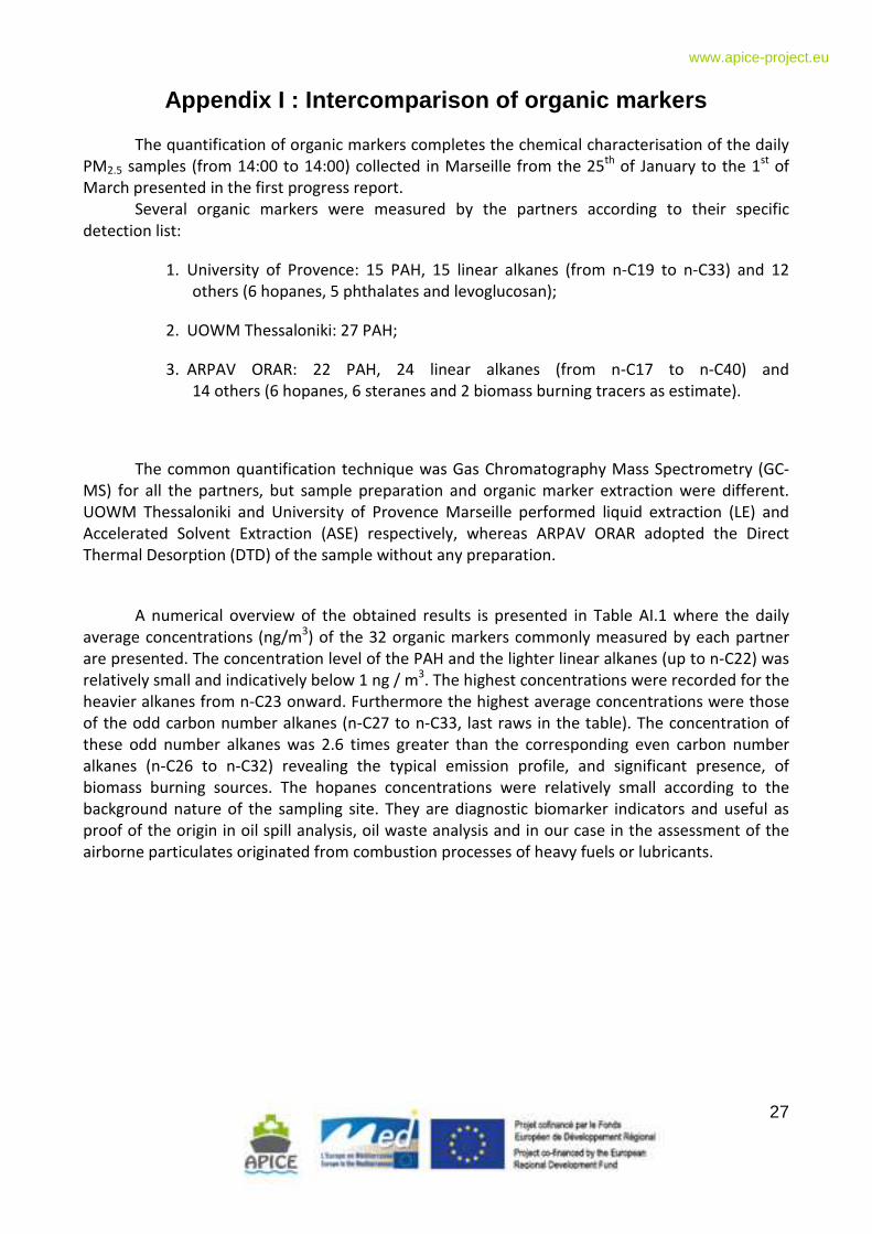
Appendix I : Intercomparison of organic markers The quantification of organic markers completes the chemical characterisation of the daily

PM2.5 samples (from 14:00 to 14:00) collected in Marseille from the 25th

of January to the 1st

of

March presented in the first progress report.

Several organic markers were measured by the partners according to their specific

detection list:

1. University of Provence: 15 PAH, 15 linear alkanes (from n-C19 to n-C33) and 12

others (6 hopanes, 5 phthalates and levoglucosan);

2. UOWM Thessaloniki: 27 PAH;

3. ARPAV ORAR: 22 PAH, 24 linear alkanes (from n-C17 to n-C40) and

14 others (6 hopanes, 6 steranes and 2 biomass burning tracers as estimate).

The common quantification technique was Gas Chromatography Mass Spectrometry (GC-

MS) for all the partners, but sample preparation and organic marker extraction were different.

UOWM Thessaloniki and University of Provence Marseille performed liquid extraction (LE) and

Accelerated Solvent Extraction (ASE) respectively, whereas ARPAV ORAR adopted the Direct

Thermal Desorption (DTD) of the sample without any preparation.

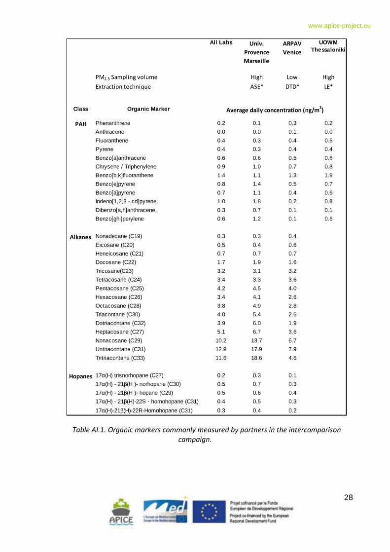
A numerical overview of the obtained results is presented in Table AI.1 where the daily

average concentrations (ng/m3) of the 32 organic markers commonly measured by each partner

are presented. The concentration level of the PAH and the lighter linear alkanes (up to n-C22) was

relatively small and indicatively below 1 ng / m3. The highest concentrations were recorded for the

heavier alkanes from n-C23 onward. Furthermore the highest average concentrations were those

of the odd carbon number alkanes (n-C27 to n-C33, last raws in the table). The concentration of

these odd number alkanes was 2.6 times greater than the corresponding even carbon number

alkanes (n-C26 to n-C32) revealing the typical emission profile, and significant presence, of

biomass burning sources. The hopanes concentrations were relatively small according to the

background nature of the sampling site. They are diagnostic biomarker indicators and useful as

proof of the origin in oil spill analysis, oil waste analysis and in our case in the assessment of the

airborne particulates originated from combustion processes of heavy fuels or lubricants.

28


All Labs Univ.

Provence

Marseille

ARPAV

Venice

UOWM Thessaloniki

PM2.5 Sampling volume High Low High

Extraction technique ASE* DTD* LE*

Class Organic Marker

PAH Phenanthrene 0.2 0.1 0.3 0.2

Anthracene 0.0 0.0 0.1 0.0

Fluoranthene 0.4 0.3 0.4 0.5

Pyrene 0.4 0.3 0.4 0.4

Benzo[a]anthracene 0.6 0.6 0.5 0.6

Chrysene / Triphenylene 0.9 1.0 0.7 0.8

Benzo[b,k]fluoranthene 1.4 1.1 1.3 1.9

Benzo[e]pyrene 0.8 1.4 0.5 0.7

Benzo[a]pyrene 0.7 1.1 0.4 0.6

Indeno[1,2,3 - cd]pyrene 1.0 1.8 0.2 0.8

Dibenzo[a,h]anthracene 0.3 0.7 0.1 0.1

Benzo[ghi]perylene 0.6 1.2 0.1 0.6

Alkanes Nonadecane (C19) 0.3 0.3 0.4

Eicosane (C20) 0.5 0.4 0.6

Heneicosane (C21) 0.7 0.7 0.7

Docosane (C22) 1.7 1.9 1.6

Tricosane(C23) 3.2 3.1 3.2

Tetracosane (C24) 3.4 3.3 3.6

Pentacosane (C25) 4.2 4.5 4.0

Hexacosane (C26) 3.4 4.1 2.6

Octacosane (C28) 3.8 4.9 2.8

Triacontane (C30) 4.0 5.4 2.6

Dotriacontane (C32) 3.9 6.0 1.9

Heptacosane (C27) 5.1 6.7 3.6

Nonacosane (C29) 10.2 13.7 6.7

Untriacontane (C31) 12.9 17.9 7.9

Tritriacontane (C33) 11.6 18.6 4.6

Hopanes 17α(H) trisnorhopane (C27) 0.2 0.3 0.1

17α(H) - 21β(H )- norhopane (C30) 0.5 0.7 0.3

17α(H) - 21β(H )- hopane (C29) 0.5 0.6 0.4

17α(H) - 21β(H)-22S - homohopane (C31) 0.4 0.5 0.3

17α(H)-21β(H)-22R-Homohopane (C31) 0.3 0.4 0.2

Average daily concentration (ng/m3)

Table AI.1. Organic markers commonly measured by partners in the intercomparison

campaign.

29


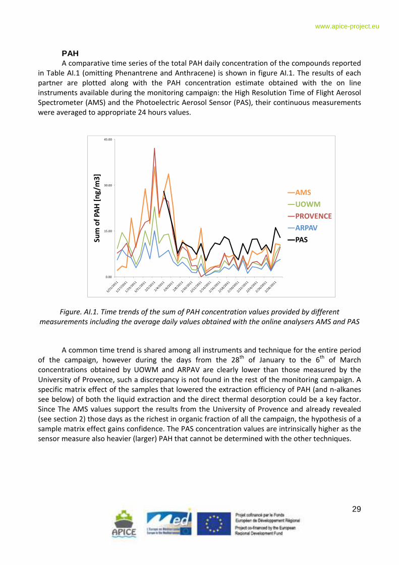
PAH A comparative time series of the total PAH daily concentration of the compounds reported

in Table AI.1 (omitting Phenantrene and Anthracene) is shown in figure AI.1. The results of each

partner are plotted along with the PAH concentration estimate obtained with the on line

instruments available during the monitoring campaign: the High Resolution Time of Flight Aerosol

Spectrometer (AMS) and the Photoelectric Aerosol Sensor (PAS), their continuous measurements

were averaged to appropriate 24 hours values.

0.00

15.00

30.00

45.00

Su

m o

f P

AH

[n

g/m

3]

AMS

UOWM

PROVENCE

ARPAV

PAS

Figure. AI.1. Time trends of the sum of PAH concentration values provided by different

measurements including the average daily values obtained with the online analysers AMS and PAS

A common time trend is shared among all instruments and technique for the entire period

of the campaign, however during the days from the 28th

of January to the 6th

of March

concentrations obtained by UOWM and ARPAV are clearly lower than those measured by the

University of Provence, such a discrepancy is not found in the rest of the monitoring campaign. A

specific matrix effect of the samples that lowered the extraction efficiency of PAH (and n-alkanes

see below) of both the liquid extraction and the direct thermal desorption could be a key factor.

Since The AMS values support the results from the University of Provence and already revealed

(see section 2) those days as the richest in organic fraction of all the campaign, the hypothesis of a

sample matrix effect gains confidence. The PAS concentration values are intrinsically higher as the

sensor measure also heavier (larger) PAH that cannot be determined with the other techniques.

30


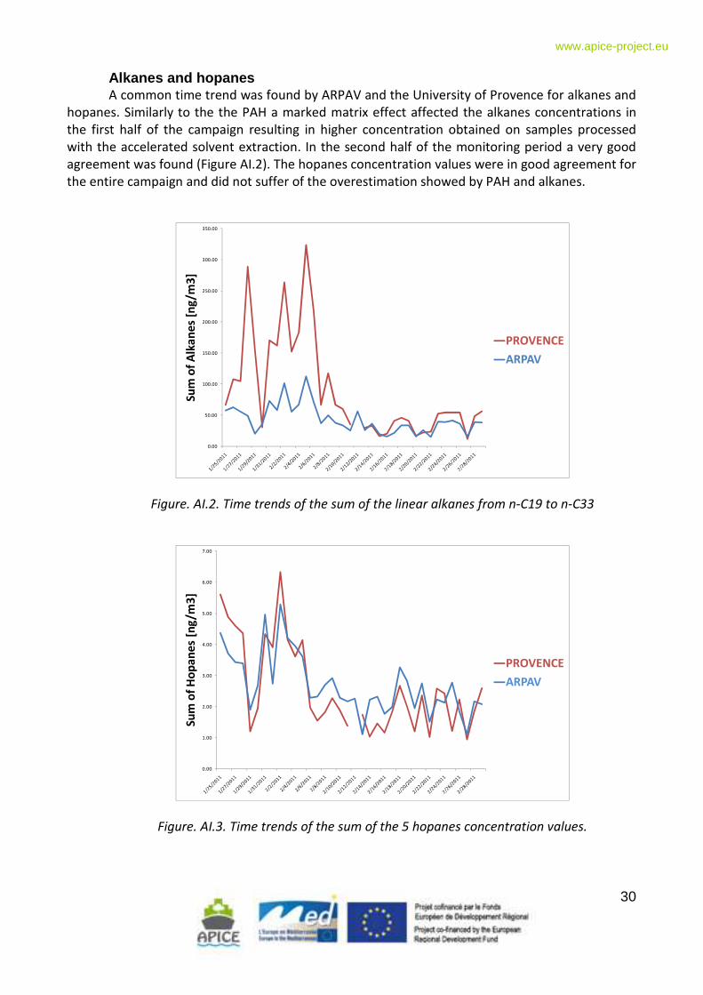
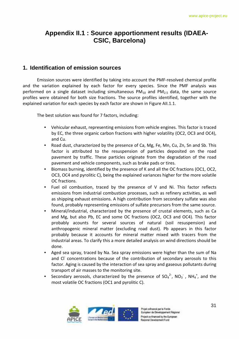
Alkanes and hopanes A common time trend was found by ARPAV and the University of Provence for alkanes and

hopanes. Similarly to the the PAH a marked matrix effect affected the alkanes concentrations in

the first half of the campaign resulting in higher concentration obtained on samples processed

with the accelerated solvent extraction. In the second half of the monitoring period a very good

agreement was found (Figure AI.2). The hopanes concentration values were in good agreement for

the entire campaign and did not suffer of the overestimation showed by PAH and alkanes.

0.00

50.00

100.00

150.00

200.00

250.00

300.00

350.00

Su

m o

f A

lka

ne

s [n

g/m

3]

PROVENCE

ARPAV

Figure. AI.2. Time trends of the sum of the linear alkanes from n-C19 to n-C33

0.00

1.00

2.00

3.00

4.00

5.00

6.00

7.00

Su

m o

f H

op

an

es

[ng

/m3

]

PROVENCE

ARPAV

Figure. AI.3. Time trends of the sum of the 5 hopanes concentration values.

31


Appendix II.1 : Source apportionment results (IDAEA -

CSIC, Barcelona)

1. Identification of emission sources

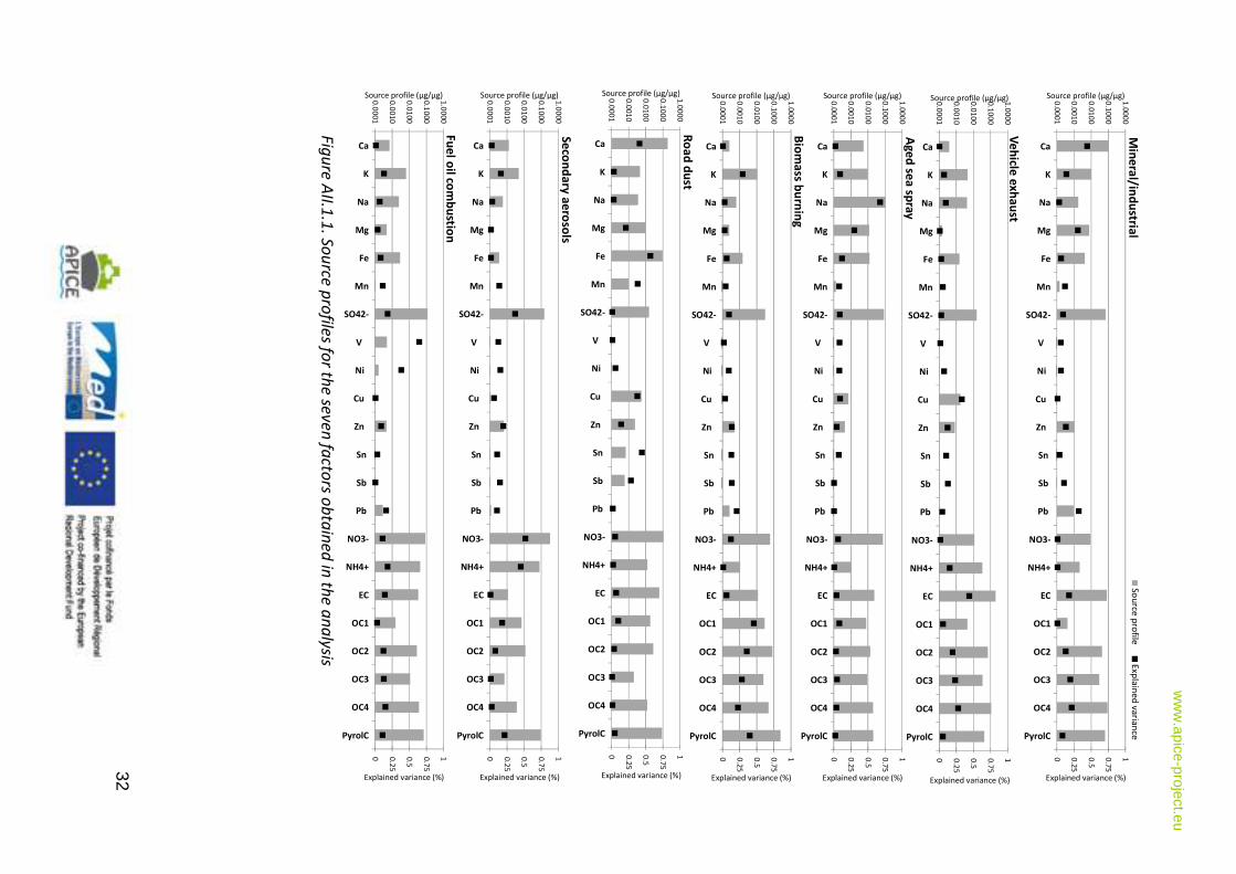
Emission sources were identified by taking into account the PMF-resolved chemical profile

and the variation explained by each factor for every species. Since the PMF analysis was

performed on a single dataset including simultaneous PM10 and PM2.5 data, the same source

profiles were obtained for both size fractions. The source profiles identified, together with the

explained variation for each species by each factor are shown in Figure AII.1.1.

The best solution was found for 7 factors, including:

• Vehicular exhaust, representing emissions from vehicle engines. This factor is traced

by EC, the three organic carbon fractions with higher volatility (OC2, OC3 and OC4),

and Cu.

• Road dust, characterized by the presence of Ca, Mg, Fe, Mn, Cu, Zn, Sn and Sb. This

factor is attributed to the resuspension of particles deposited on the road

pavement by traffic. These particles originate from the degradation of the road

pavement and vehicle components, such as brake pads or tires.

• Biomass burning, identified by the presence of K and all the OC fractions (OC1, OC2,

OC3, OC4 and pyrolitic C), being the explained variances higher for the more volatile

OC fractions.

• Fuel oil combustion, traced by the presence of V and Ni. This factor reflects

emissions from industrial combustion processes, such as refinery activities, as well

as shipping exhaust emissions. A high contribution from secondary sulfate was also

found, probably representing emissions of sulfate precursors from the same source.

• Mineral/industrial, characterized by the presence of crustal elements, such as Ca

and Mg, but also Pb, EC and some OC fractions (OC2, OC3 and OC4). This factor

probably acounts for several sources of natural (soil resuspension) and

anthropogenic mineral matter (excluding road dust). Pb appears in this factor

probably because it accounts for mineral matter mixed with tracers from the

industrial areas. To clarify this a more detailed analysis on wind directions should be

done.

• Aged sea spray, traced by Na. Sea spray emissions were higher than the sum of Na

and Cl-

concentrations because of the contribution of secondary aerosols to this

factor. Aging is caused by the interaction of sea spray and gaseous pollutants during

transport of air masses to the monitoring site.

• Secondary aerosols, characterized by the presence of SO42-

, NO3-

, NH4+, and the

most volatile OC fractions (OC1 and pyrolitic C).

32

ww

w.apice-project.eu

0 0.2

5

0.5

0.7

5

1

0.0

00

1

0.0

01

0

0.0

10

0

0.1

00

0

1.0

00

0

Ca

K

Na

Mg

Fe

Mn

SO42-

V

Ni

Cu

Zn

Sn

Sb

Pb

NO3-

NH4+

EC

OC1

OC2

OC3

OC4

PyrolC

Explained variance (%)

Source profile (µg/µg)M

ine

ral/in

du

strial

So

urce

pro

fileE

xpla

ine

d v

aria

nce

0 0.2

5

0.5

0.7

5

1

0.0

00

1

0.0

01

0

0.0

10

0

0.1

00

0

1.0

00

0

Ca

K

Na

Mg

Fe

Mn

SO42-

V

Ni

Cu

Zn

Sn

Sb

Pb

NO3-

NH4+

EC

OC1

OC2

OC3

OC4

PyrolC


Source profile (µg/µg)

Ve

hicle

ex

ha

ust

0 0.2

5

0.5

0.7

5

1

0.0

00

1

0.0

01

0

0.0

10

0

0.1

00

0

1.0

00

0

Ca

K

Na

Mg

Fe

Mn

SO42-

V

Ni

Cu

Zn

Sn

Sb

Pb

NO3-

NH4+

EC

OC1

OC2

OC3

OC4

PyrolC



Ag

ed

sea

spra

y

0 0.2

5

0.5

0.7

5

1

0.0

00

1

0.0

01

0

0.0

10

0

0.1

00

0

1.0

00

0

Ca

K

Na

Mg

Fe

Mn

SO42-

V

Ni

Cu

Zn

Sn

Sb

Pb

NO3-

NH4+

EC

OC1

OC2

OC3

OC4

PyrolC



Bio

ma

ss bu

rnin

g

0 0.2

5

0.5

0.7

5

1

0.0

00

1

0.0

01

0

0.0

10

0

0.1

00

0

1.0

00

0

Ca

K

Na

Mg

Fe

Mn

SO42-

V

Ni

Cu

Zn

Sn

Sb

Pb

NO3-

NH4+

EC

OC1

OC2

OC3

OC4

PyrolC



Ro

ad

du

st

0 0.2

5

0.5

0.7

5

1

0.0

00

1

0.0

01

0

0.0

10

0

0.1

00

0

1.0

00

0

Ca

K

Na

Mg

Fe

Mn

SO42-

V

Ni

Cu

Zn

Sn

Sb

Pb

NO3-

NH4+

EC

OC1

OC2

OC3

OC4

PyrolC



Se

con

da

ry a

ero

sols

0 0.2

5

0.5

0.7

5

1

0.0

00

1

0.0

01

0

0.0

10

0

0.1

00

0

1.0

00

0

Ca

K

Na

Mg

Fe

Mn

SO42-

V

Ni

Cu

Zn

Sn

Sb

Pb

NO3-

NH4+

EC

OC1

OC2

OC3

OC4

PyrolC



Fue

l oil co

mb

ustio

n

F

igu

re A

II.1.1

. So

urce

pro

files fo

r the

seve

n fa

ctors o

bta

ine

d in

the

an

aly

sis

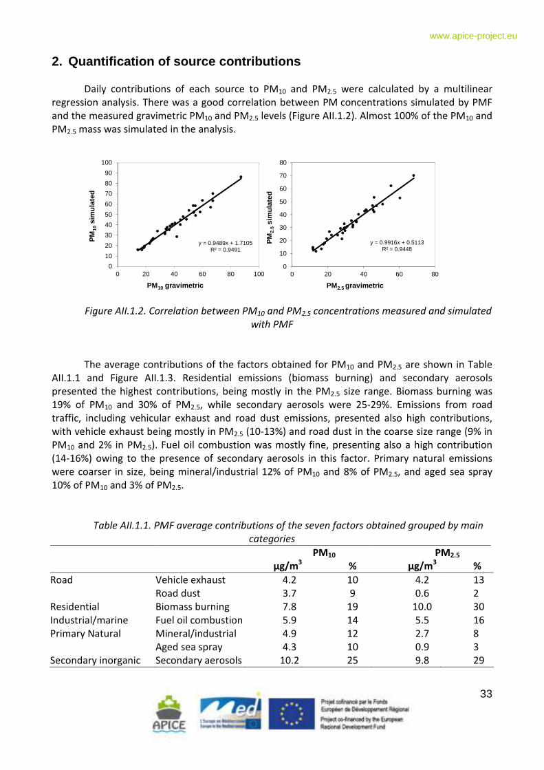
33


2. Quantification of source contributions

Daily contributions of each source to PM10 and PM2.5 were calculated by a multilinear

regression analysis. There was a good correlation between PM concentrations simulated by PMF

and the measured gravimetric PM10 and PM2.5 levels (Figure AII.1.2). Almost 100% of the PM10 and

PM2.5 mass was simulated in the analysis.

y = 0.9489x + 1.7105R² = 0.9491

0

10

20

30

40

50

60

70

80

90

100

0 20 40 60 80 100

PM

10si

mul

ated

PM10 gravimetric

y = 0.9916x + 0.5113R² = 0.9448

0

10

20

30

40

50

60

70

80

0 20 40 60 80P

M2.

5si

mul

ated

PM2.5 gravimetric

Figure AII.1.2. Correlation between PM10 and PM2.5 concentrations measured and simulated

with PMF

The average contributions of the factors obtained for PM10 and PM2.5 are shown in Table

AII.1.1 and Figure AII.1.3. Residential emissions (biomass burning) and secondary aerosols

presented the highest contributions, being mostly in the PM2.5 size range. Biomass burning was

19% of PM10 and 30% of PM2.5, while secondary aerosols were 25-29%. Emissions from road

traffic, including vehicular exhaust and road dust emissions, presented also high contributions,

with vehicle exhaust being mostly in PM2.5 (10-13%) and road dust in the coarse size range (9% in

PM10 and 2% in PM2.5). Fuel oil combustion was mostly fine, presenting also a high contribution

(14-16%) owing to the presence of secondary aerosols in this factor. Primary natural emissions

were coarser in size, being mineral/industrial 12% of PM10 and 8% of PM2.5, and aged sea spray

10% of PM10 and 3% of PM2.5.

Table AII.1.1. PMF average contributions of the seven factors obtained grouped by main

categories

PM10 PM2.5

µg/m3

% µg/m3 %

Road Vehicle exhaust 4.2 10 4.2 13

Road dust 3.7 9 0.6 2

Residential Biomass burning 7.8 19 10.0 30

Industrial/marine Fuel oil combustion 5.9 14 5.5 16

Primary Natural Mineral/industrial 4.9 12 2.7 8

Aged sea spray 4.3 10 0.9 3

Secondary inorganic Secondary aerosols 10.2 25 9.8 29

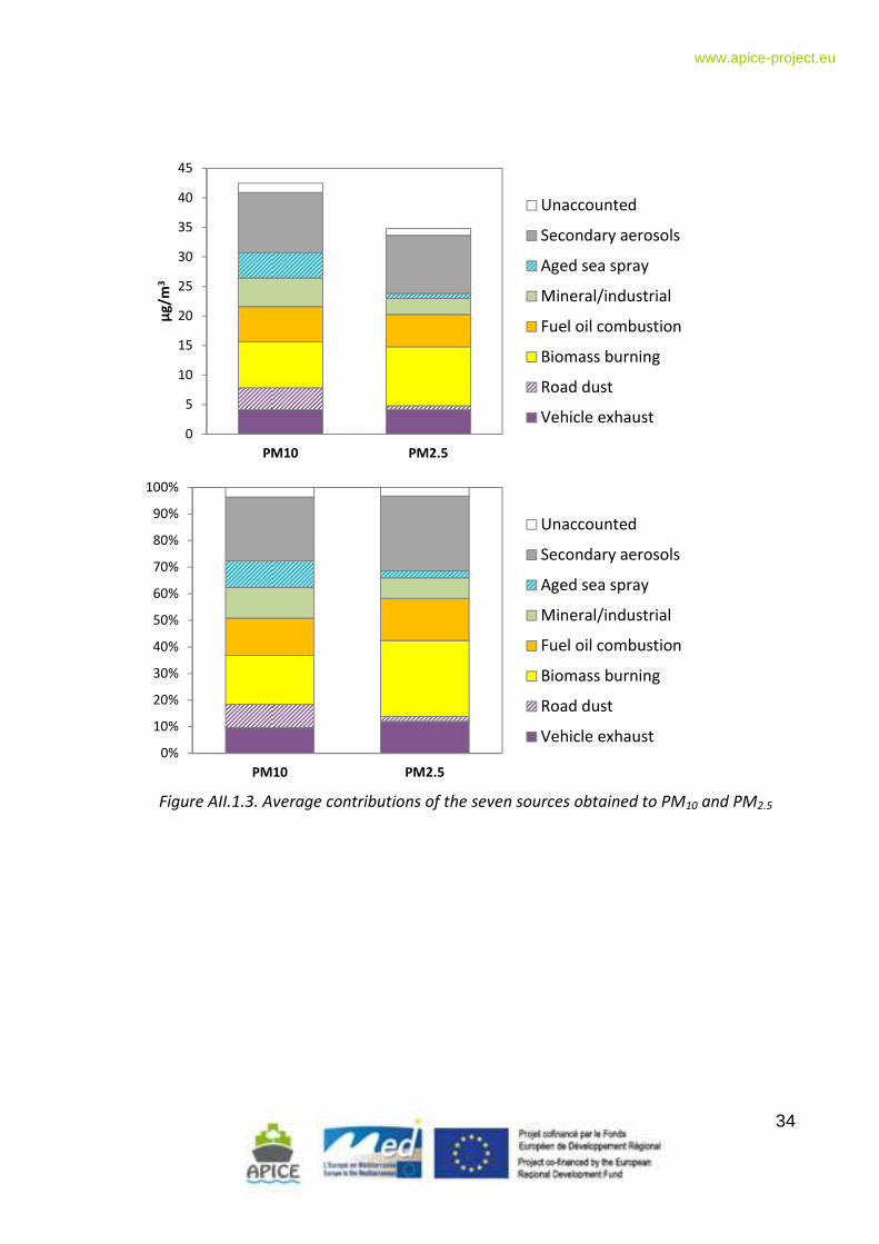
34


0

5

10

15

20

25

30

35

40

45

PM10 PM2.5

µg

/m3

Unaccounted

Secondary aerosols

Aged sea spray

Mineral/industrial

Fuel oil combustion

Biomass burning

Road dust

Vehicle exhaust

0%

10%

20%

30%

40%

50%

60%

70%

80%

90%

100%

PM10 PM2.5

Unaccounted

Secondary aerosols

Aged sea spray

Mineral/industrial

Fuel oil combustion

Biomass burning

Road dust

Vehicle exhaust

Figure AII.1.3. Average contributions of the seven sources obtained to PM10 and PM2.5

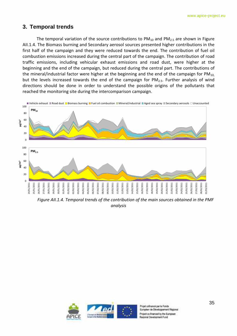
35


3. Temporal trends

The temporal variation of the source contributions to PM10 and PM2.5 are shown in Figure

AII.1.4. The Biomass burning and Secondary aerosol sources presented higher contributions in the

first half of the campaign and they were reduced towards the end. The contribution of fuel oil

combustion emissions increased during the central part of the campaign. The contribution of road

traffic emissions, including vehicular exhaust emissions and road dust, were higher at the

beginning and the end of the campaign, but reduced during the central part. The contributions of

the mineral/industrial factor were higher at the beginning and the end of the campaign for PM10,

but the levels increased towards the end of the campaign for PM2.5. Further analysis of wind

directions should be done in order to understand the possible origins of the pollutants that

reached the monitoring site during the intercomparison campaign.

0

20

40

60

80

100

µg

/m3

PM10

Vehicle exhaust Road dust Biomass burning Fuel oil combustion Mineral/industrial Aged sea spray Secondary aerosols Unaccounted

0

20

40

60

80

100

24

/01

/20

11

25

/01

/20

11

26

/01

/20

11

27

/01

/20

11

28

/01

/20

11

29

/01

/20

11

30

/01

/20

11

31

/01

/20

11

01

/02

/20

11

02

/02

/20

11

03

/02

/20

11

04

/02

/20

11

05

/02

/20

11

06

/02

/20

11

07

/02

/20

11

08

/02

/20

11

09

/02

/20

11

10

/02

/20

11

11

/02

/20

11

12

/02

/20

11

13

/02

/20

11

14

/02

/20

11

15

/02

/20

11

16

/02

/20

11

17

/02

/20

11

18

/02

/20

11

19

/02

/20

11

20

/02

/20

11

21

/02

/20

11

22

/02

/20

11

23

/02

/20

11

24

/02

/20

11

25

/02

/20

11

26

/02

/20

11

27

/02

/20

11

28

/02

/20

11

01

/03

/20

11

µg

/m3

PM2.5

Figure AII.1.4. Temporal trends of the contribution of the main sources obtained in the PMF

analysis

36


References

Amato, F., Pandolfi, M., Escrig, A., Querol, X., Alastuey, A., Pey, J., Perez, N., Hopke, P. K., 2009.

Quantifying road dust resuspension in urban environment by multilinear engine: a

comparison with PMF2. Atmospheric Environment 43, 2770-2780.

Cavalli F., Viana M., Yttri K. E., Genberg J. and Putaud J. P. (2010). Toward a standardised thermal-

optical protocol for measuring atmospheric organic and elemental carbon: the EUSAAR

protocol. Atmos. Meas. Tech., 3, 1, 79-89.

Escrig, A., Monfort, E., Celades, I., Querol, X., Amato, F., Minguillon, M.C., Hopke, P., 2009.

Application of optimally scaled target factor analysis for assessing source contribution of

ambient PM10. Journal of the Air & Waste Management Association 59, 1296-1307.

Paatero, P.; Tapper, U. Positive Matrix Factorization: a Non-Negative Factor Model with Optimal

Utilization of Error Estimates of Data Values; Environmetrics 1994, 5, 111-126.

Paatero, P. Least Squares Formulation of Robust Non-Negative Factor Analysis; Chemom. Intell.

Lab. Syst. 1997, 37, 23-35.

Paatero, P., Hopke, P.K., 2003. Discarding or downweighting high-noise variables in factor analytic

models. Analytica Chimica Acta 490 (1-2, 25), 277-289.

37


Appendix II.2 : Source apportionment results (Univ Genoa, Genoa)

1. Methodology of sampling and methods of analysis

During the experimental campaign, carried out in Marseille from 25/1/2011 to 28/02/2011,

PM2.5 sampling was performed. The filters (54 samples) were collected by standard Low Volume

(Tecora), on 47 mm Quartz and Teflon filters, changed and alternated every 12 hours still

beginning at 2.00 pm. Our sampling are different from all the other groups/Institutions for the

type of filters and the time-basis of PM sampling.

The compositional analysis, performed by Genoa’s group for samples collected in this campaign,

was conducted with different chemical-physical methods and PM compounds measured are:

• 18 elements: Na, Mg, Al, Si, P, K, Ca, Ti, V, Cr, Mn, Fe, Ni, Cu, Zn, Br, Mo, Pb

• 8 ions: Cl-, NO3

-, SO4

2-, Na

+, NH4

+, K

+, Mg

+, Ca

2+

• Organic & Elemental Carbon: OC, EC

Elemental concentrations were obtained with Energy Dispersive X- ray Fluorescence, ED-

XRF, a widespread and versatile technique for the quantification of the elements present in a

sample, and even traces therefore (Tsuji et al, 2004) but with atomic number Z>10. ED-XRF is

based on the ionization of the inner atomic shells obtained by irradiating the samples with

electromagnetic radiation: inner shell vacancies get promptly filled by outer shell electrons, with

the release of radiant energy. During the de-excitation, energy is released under the form of

fluorescence in the X-band: emitted photon energies equal the energy differences between outer

and inner shells, and thus carry the signature of the emitting atom. The peak positions in the

energy spectrum allow the identification of the elements present in the sample and the peak areas

are proportional to concentrations.

Ionic fraction was analysed with Ion Chromatography, in collaboration with "Dipartimento

di Chimica Inorganica, Metallorganica e Analitica dell’Università degli Studi di Milano". Ion

Chromatography (IC) is a physical-chemical separation technique that provides quantitative

analysis of inorganic ions from a complex mixture. IC combines features of ion exchange, liquid

chromatography, eluent suppression, and quantitative detection. IC has multispecies capabilities,

small sample requirements, and the detectors have high sensibility, variable selectivity, good

stability and high linearity of response.

The quantification of OC and EC fractions was obtained by the Thermal-Optical

Transmittance method (SUNSET system - Birch and Cary, 1996) consisting of two main steps. In

the first part of the analysis, during the evolution in inert atmosphere, pyrolysis of the material

deposited on the filter can occur and in extreme condition to form EC (Chow et al, 2007). In this

condition, pyrolysed OC (PyC) cannot evolve in the inert atmosphere anymore, thus an

underestimation of OC and an overestimation of EC are registered. Pyrolysis leads to the variation

of the optical proprieties of the sample as PyC is light-adsorbing; thus, in the TOT analysis, the

optical transmission of a laser thought the filter is continuously monitored. Due to pyrolysis, the

transmittance of the filter decreases during the first part of the analysis (He atmosphere). When

oxygen is injected into the line, EC (both originally present on the filter and derived from OC

pyrolysis) evolves causing an increase of the laser transmission. When the filter transmittance

38


reaches the values registered at the beginning of the analysis, the method assumes that a quantity

of EC equal to the one formed by pyrolysis has combusted and therefore all the carbon evolved up

to this point has to be considered OC. All remaining carbon is considered EC. This method does not

physically separate the two fraction, but it simply corrects the measured concentration using EC

optical proprieties.

This experimental sampling strategy presented some problems: the light elements (Na to

P) were not detectable by ED-XRF on quartz filters and EC/OC concentration values were available

each two days (i.e. only on quartz filters). For this reason, the light absorption and thence the BC

content in the PM collected with the PTFE filters, was measured off-line by a simple, fully

automatic and non-destructive new optical system developed in our laboratory.

2. Source apportionment approach

The source apportionment approach used by Genoa’s group is the Positive Matrix

Factorization version 2 (PMF2). PMF2 is an advanced receptor model, developed by Paatero and

Hopke (Paatero et al, 1994). In the last years this approach has been asserted like most reliable to

international level. It is useful, especially, where detailed data do not exist on the composition of

the main emission sources, but where large numbers of sampled data are available on ambient

concentrations. The important advantage of the positive matrix factorization is the ability to

handle missing data and values below the detection limits data by adjusting the error estimates of

each data point. In fact, the solution to the PMF problem depends on the uncertainties attributed

to each value.

The concentrations values and their associated errors were treated according to Polissar et al.

(Polissar et al, 1998). Values corresponding to one half of detection limit were used for data below

detection limits in the calculations of geometric means (Table AII.2.1).

Table AII.2.1: approach suggested by Polissar et al, 1998 for the concentration values and

their associated error estimates

Another important aspect of data points weighting, is the handling of extreme values.

Environmental data typically show a positively skewed distribution; often with a long tail. Thus,

there can be extreme values in the distribution as well as true “outliers”. In either case, such high

values would have significant influence on the solution: this influence will generally distort the

solution and thus, an approach to reduce their influence can be an useful tool. In this approach,

we used PMF in “robust mode”: the robust factorization, based on the Huber influence function

(Huber, 1981), is a technique of iterative reweighing of the individual data values.

Mass apportionment was calculated both performing a linear regression between the

temporal trends of sources resolved by PMF and the time trends of mass concentrations

(Ramadan et al., 2000) and including PM mass concentration as an independent variable in PMF

geometrica media~ con~4, : valuesMissing

32,

2x:MDL below Values

3,: valuesDetermined

ij

jjijjij

ijj

ijij

ijijijijij

ccscx

MDLMDLs

MDL

MDLscx

==

+==

+== σ

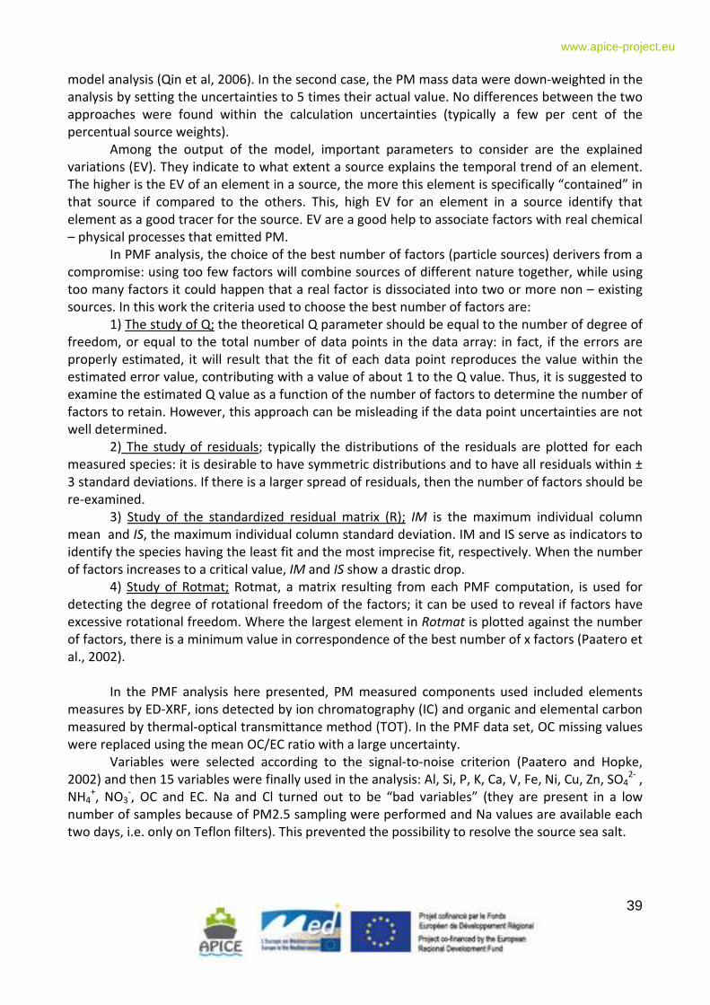
39


model analysis (Qin et al, 2006). In the second case, the PM mass data were down-weighted in the

analysis by setting the uncertainties to 5 times their actual value. No differences between the two

approaches were found within the calculation uncertainties (typically a few per cent of the

percentual source weights).

Among the output of the model, important parameters to consider are the explained

variations (EV). They indicate to what extent a source explains the temporal trend of an element.

The higher is the EV of an element in a source, the more this element is specifically “contained” in

that source if compared to the others. This, high EV for an element in a source identify that

element as a good tracer for the source. EV are a good help to associate factors with real chemical

– physical processes that emitted PM.

In PMF analysis, the choice of the best number of factors (particle sources) derivers from a

compromise: using too few factors will combine sources of different nature together, while using

too many factors it could happen that a real factor is dissociated into two or more non – existing

sources. In this work the criteria used to choose the best number of factors are:

1) The study of Q; the theoretical Q parameter should be equal to the number of degree of

freedom, or equal to the total number of data points in the data array: in fact, if the errors are

properly estimated, it will result that the fit of each data point reproduces the value within the

estimated error value, contributing with a value of about 1 to the Q value. Thus, it is suggested to

examine the estimated Q value as a function of the number of factors to determine the number of

factors to retain. However, this approach can be misleading if the data point uncertainties are not

well determined.

2) The study of residuals; typically the distributions of the residuals are plotted for each

measured species: it is desirable to have symmetric distributions and to have all residuals within ±

3 standard deviations. If there is a larger spread of residuals, then the number of factors should be

re-examined.

3) Study of the standardized residual matrix (R); IM is the maximum individual column

mean and IS, the maximum individual column standard deviation. IM and IS serve as indicators to

identify the species having the least fit and the most imprecise fit, respectively. When the number

of factors increases to a critical value, IM and IS show a drastic drop.

4) Study of Rotmat; Rotmat, a matrix resulting from each PMF computation, is used for

detecting the degree of rotational freedom of the factors; it can be used to reveal if factors have

excessive rotational freedom. Where the largest element in Rotmat is plotted against the number

of factors, there is a minimum value in correspondence of the best number of x factors (Paatero et

al., 2002).

In the PMF analysis here presented, PM measured components used included elements

measures by ED-XRF, ions detected by ion chromatography (IC) and organic and elemental carbon

measured by thermal-optical transmittance method (TOT). In the PMF data set, OC missing values

were replaced using the mean OC/EC ratio with a large uncertainty.


2002) and then 15 variables were finally used in the analysis: Al, Si, P, K, Ca, V, Fe, Ni, Cu, Zn, SO42-

,

NH4+, NO3

-, OC and EC. Na and Cl turned out to be “bad variables” (they are present in a low

number of samples because of PM2.5 sampling were performed and Na values are available each

two days, i.e. only on Teflon filters). This prevented the possibility to resolve the source sea salt.

40


3. Results

The number of factors which was examined ranged from three to eight. Finally, five sources

were resolved and labeled, according to their characteristic tracers, as follows: Road (traced by

Cu), Dust (traced by Al, Si, Ca), Industrial/Marin (Oil Combustion traced by V, Ni), Secondary

Compounds (Secondary I traced by SO42-

and NH4+

and Secondary II traced by NO3- and NH4

+). PMF

applied to a time series of elemental concentration values resolved, over the number, the profiles

of PM sources at the sampling site (Figure AII.2.1) and their contribution to PM2.5 levels (Figure

2). In Figure 3 the correlation between measured and calculated mass is shown to validate the

results of PMF analysis.

The source profiles deserve some specific comments:

• Road: This source is linked to road traffic.

• Secondary: Species measured in this experiment (ions, organic and elemental carbon)

make it possible to separate Secondary Compounds into two different sources, the first

traced by sulfates and ammonium (hereinafter called Secondary I) and the second one

traced by nitrates (hereinafter called Secondary II). The concentration ratio SO42-

/NH4+ in

Secondary I is 2.3 ± 0.2, in agreement with the stoechiometric ratio. Secondary II presents a

concentration ratio NO3-/NH4

+ of 2.8 ± 0.3, in partial agreement with stoechiometric ratio.

• Industrial/Marine: This source is linked to Oil Combustion and the V/Ni concentration ratio

in the profile is 2.5 ± 0.3. This profile presents an high contribution of SO42-

and NH4+

(concentration ratio SO4--/NH4

+ is 2.2 ± 0.2), due to an only partial separation obtained by

PMF analysis between this source and Secondary I.

• Dust: PMF analysis resolves a source partially natural. It is a source that includes both soil

and soil re-suspended from road traffic. In fact, the concentration ratios of soil tracers

(Al:Si and Al:Ca) in the profile are in disagreement with the literature values (Mason, 1966).

This confirms the hypothesis that this source is only partially natural and that its

composition is significantly contaminated by anthropogenic source emissions.

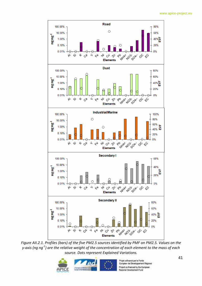
41


Figure AII.2.1. Profiles (bars) of the five PM2.5 sources identified by PMF on PM2.5. Values on the

y-axis (ng ng-1

) are the relative weight of the concentration of each element to the mass of each

source. Dots represent Explained Variations.

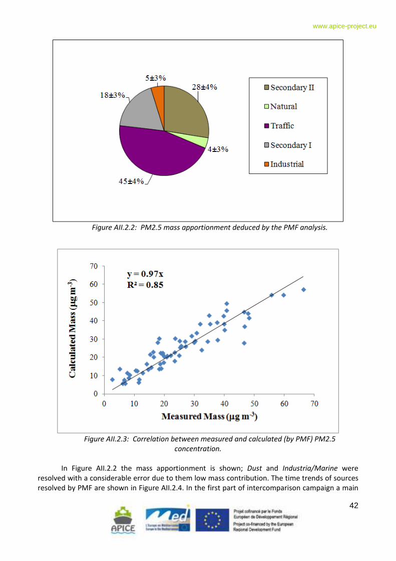
42


Figure AII.2.2: PM2.5 mass apportionment deduced by the PMF analysis.

Figure AII.2.3: Correlation between measured and calculated (by PMF) PM2.5

concentration.

In Figure AII.2.2 the mass apportionment is shown; Dust and Industria/Marine were

resolved with a considerable error due to them low mass contribution. The time trends of sources

resolved by PMF are shown in Figure AII.2.4. In the first part of intercomparison campaign a main

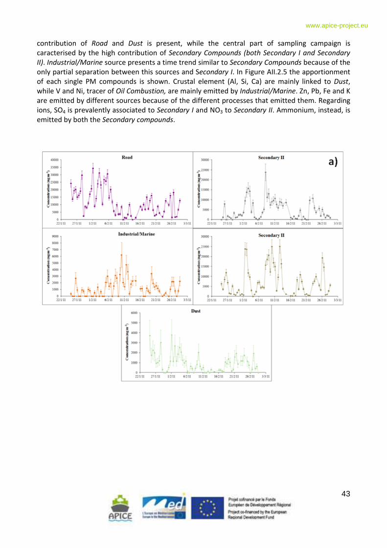
43


contribution of Road and Dust is present, while the central part of sampling campaign is

caracterised by the high contribution of Secondary Compounds (both Secondary I and Secondary

II). Industrial/Marine source presents a time trend similar to Secondary Compounds because of the

only partial separation between this sources and Secondary I. In Figure AII.2.5 the apportionment

of each single PM compounds is shown. Crustal element (Al, Si, Ca) are mainly linked to Dust,

while V and Ni, tracer of Oil Combustion, are mainly emitted by Industrial/Marine. Zn, Pb, Fe and K

are emitted by different sources because of the different processes that emitted them. Regarding

ions, SO4 is prevalently associated to Secondary I and NO3 to Secondary II. Ammonium, instead, is

emitted by both the Secondary compounds.

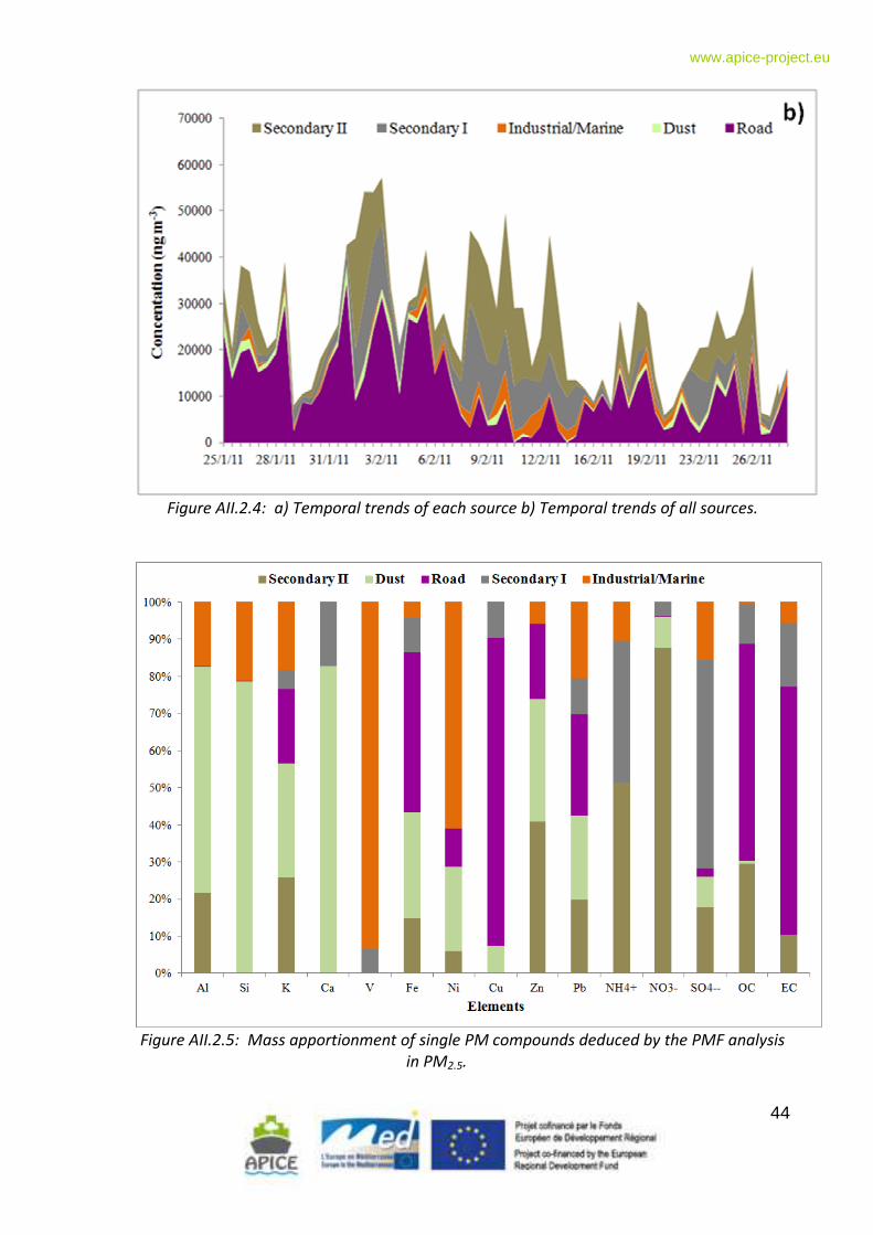
44


Figure AII.2.4: a) Temporal trends of each source b) Temporal trends of all sources.

Figure AII.2.5: Mass apportionment of single PM compounds deduced by the PMF analysis

in PM2.5.

45


References

Birch M.E. and Cary R.A., 1996. Elemental Carbon-basedn method for monitoring occupational

exposures to particulate diesel exhaust. Aerosol Science and Technology 25, 221-241.

Chow, J.C., Yu, J.Z., Watson, J.G., Hang, S.S., Bohannan, T.L., Hays, M.D., Fung, K.K., 2007. The

application of thermal methods for determining chemical composition of carbonaceous

aerosols: A review. Journal of Environmental Science and Health Part A 42, 1521-1541.

Huber P.J., 1981. Robust Statistics. John Wiley and Sons.

Mason, B., 1966. Principles of Geochemistry. Wiley, New York.

Paatero, P., Tapper, U., 1994. Positive Matrix Factorization: a non-negative factor model with

optimal utilization of error estimates of data values. Environmetrics 5, 111-126.

Paatero, P., Hopke, P.K., Song, X.H., Ramadan, Z., 2002. Understanding and controlling rotations in

factor analytic models. Chemiometrics and Intelligence Laboratory System 60, 253-264.

Polissar, A.V., Hopke, P.K., Paatero, P., Malm, W.C. Sisler, J.F., 1998. Atmospheric aerosol

nucleation and primary emission rates. Atmospheric Chemistry and Physics, 1339-1356.

Qin, Y., Kim, E., Hopke, P.K., 2006.The concentration and sources of PM2.5 in metropolitan New

York City. Atmospheric Environment 40, 312-332.

Ramadan, Z., Song, X.H, Hopke, P.K., 2003. Identification of sources of Phoenix aerosol by positive

matrix factorization. Journal of Air and Waste Management Association 50, 1308-1320

Tsuji, K., Injuk, J., Van Grieken, R., 2004. X-ray spectrometry: recent technological advances. John

Wiley and Sons.

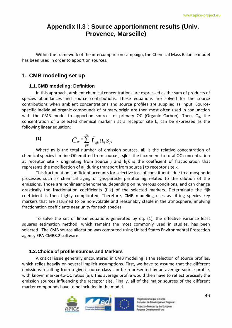
46


Appendix II.3 : Source apportionment results (Univ. Provence, Marseille)

Within the framework of the intercomparison campaign, the Chemical Mass Balance model

has been used in order to apportion sources.

1. CMB modeling set up

1.1. CMB modeling: Definition In this approach, ambient chemical concentrations are expressed as the sum of products of

species abundances and source contributions. These equations are solved for the source

contributions when ambient concentrations and source profiles are supplied as input. Source-

specific individual organic compounds of primary origin are then most often used in conjunction

with the CMB model to apportion sources of primary OC (Organic Carbon). Then, Cik, the

concentration of a selected chemical marker i at a receptor site k, can be expressed as the

following linear equation:

(1)

Where m is the total number of emission sources, aij is the relative concentration of

chemical species i in fine OC emitted from source j, sjk is the increment to total OC concentration

at receptor site k originating from source j and fijk is the coefficient of fractionation that

represents the modification of aij during transport from source j to receptor site k.

This fractionation coefficient accounts for selective loss of constituent i due to atmospheric

processes such as chemical aging or gas-particle partitioning related to the dilution of the

emissions. Those are nonlinear phenomena, depending on numerous conditions, and can change

drastically the fractionation coefficients (fijk) of the selected markers. Determinate the fijk

coefficient is then highly complicated. Therefore, CMB modeling uses as fitting species key

markers that are assumed to be non-volatile and reasonably stable in the atmosphere, implying

fractionation coefficients near unity for such species.

To solve the set of linear equations generated by eq. (1), the effective variance least

squares estimation method, which remains the most commonly used in studies, has been

selected. The CMB source allocation was computed using United States Environmental Protection

agency EPA-CMB8.2 software.

1.2. Choice of profile sources and Markers A critical issue generally encountered in CMB modeling is the selection of source profiles,

which relies heavily on several implicit assumptions. First, we have to assume that the different

emissions resulting from a given source class can be represented by an average source profile,

with known marker-to-OC ratios (aij). This average profile would then have to reflect precisely the

emission sources influencing the receptor site. Finally, all of the major sources of the different

marker compounds have to be included in the model.

∑=

=m

jjkijijkik safC

1

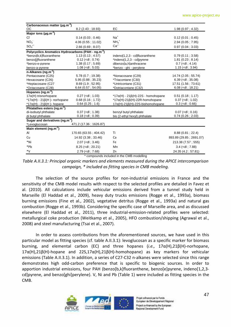
47


OC 8.2 (2.43 ; 18.93) EC 1.98 (0.97 ; 4.32)

Cl- 0.14 (0.03 ; 0.46) Na+ 0.12 (0.01 ; 0.45)NO3

- 4.06 (0.55 ; 11.02) NH4+ 2.94 (0.05 ; 7.95)

SO42-

2.66 (0.69 ; 8.07) Ca2+0.97 (0.04 ; 3.03)

*benzo[b,k]fluoranthene 1.13 (0.13 ; 4.57) indeno[1,2,3 - cd]fluoranthene 0.79 (0.11 ; 3.58)benzo[j]fluoranthene 0.12 (<dl ; 0.74) *indeno[1,2,3 - cd]pyrene 1.81 (0.23 ; 8.14)*benzo-e-pyrene 1.38 (0.17 ; 5.69) dibenzo[a,h]anthracene 0.7 (<dl ; 4.14)benzo-a-pyrene 1.08 (<dl ; 5.03) *benzo - ghi - perylene 1.15 (<dl ; 3.94)

Pentacosane (C25) 5.78 (0.7 ; 19.38) *Nonacosane (C29) 14.74 (2.05 ; 55.74)Hexacosane (C26) 5.95 (0.88 ; 35.23) *Triacontane (C30) 6.39 (<dl ; 35.08)*Heptacosane (C27 8.69 (1.9 ; 52.95) *Untricontane (C31) 17.51 (1.56 ; 73.61)*Octacosane (C28) 6.64 (0.57 ; 54.05) *Dotriacontane (C32) 6.08 (<dl ; 18.21)

17α(H) trisnorhopane 0.27 (<dl ; 1.03) *17α(H) - 21β(H)-22S - homohopane 0.51 (0.18 ; 1.17)*17α(H) - 21β(H )- norhopane 0.68 (0.16 ; 1.72) *17α(H)-21β(H)-22R-homohopane 0.37 (<dl ; 1.02)*17α(H) - 21β(H )- hopane 0.64 (0.25 ; 1.6) 17α(H)-21β(H)-22S-bishomohopane 0.3 (<dl ; 0.66)

di-isobutyl phthalate 0.37 (<dl ; 1.38) benzyl butyl phthalate 0.07 (<dl ; 0.16)di butyl phthalate 0.18 (<dl ; 0.39) bis (2-ethyl hexyl) phthalate 0.74 (0.26 ; 2.03)

*Levoglucosan 471.2 (17.36 ; 1626.87)

Al 170.65 (63.55 ; 404.42) Ti 8.88 (0.81 ; 22.4)Cu 14.92 (3.38 ; 33.46) Ca 893.89 (29.85 ; 2691.07)*Ni 2.07 (<dl ; 3.46) Fe 213.38 (7.57 ; 555)

*Pb 8.25 (<dl ; 20.21) Mn 3.4 (<dl ; 7.88)*V 2.79 (<dl ; 7.68) Zn 24.35 (4.2 ; 57.81)

* compounds included in the CMB modelling

Hopanes (ng.m -3)

Phtalathes esters (ng.m -3)

Sugar and derivatives (ng.m -3)

Main element (ng.m -3)

Carbonaceous matter (µg.m-3)

Major ions (µg.m-3)

Polycyclics Aromatics Hydrocarbons (PAH - ng.m -3)

n-Alkanes (ng.m -3)

Table A.II.3.1: Principal organic markers and elements measured during the APICE intercomparison

campaign, * included as fitting species in CMB modeling.

The selection of the source profiles for non-industrial emissions in France and the

sensitivity of the CMB model results with respect to the selected profiles are detailed in Favez et

al. (2010). All calculations include vehicular emissions derived from a tunnel study held in

Marseille (El Haddad et al., 2009), heavy duty trucks emissions (Rogge et al., 1993a), biomass

burning emissions (Fine et al., 2002), vegetative detritus (Rogge et al., 1993a) and natural gas

combustion (Rogge et al., 1993b). Considering the specific case of Marseille area, and as discussed

elsewhere (El Haddad et al., 2011), three industrial-emission-related profiles were selected:

metallurgical coke production (Weitkamp et al., 2005), HFO combustion/shipping (Agrawal et al.,

2008) and steel manufacturing (Tsai et al., 2007).

In order to assess contributions from the aforementioned sources, we have used in this

particular model as fitting species (cf. table A.II.3.1): levoglucosan as a specific marker for biomass

burning, and elemental carbon (EC) and three hopanes (i.e., 17α(H),21β(H)-norhopane,

17α(H),21β(H)-hopane and 22S,17α(H),21β(H)-homohopane) as key markers for vehicular

emissions (Table A.II.3.1). In addition, a series of C27-C32 n-alkanes were selected since this range

demonstrates high odd-carbon preference that is specific to biogenic sources. In order to

apportion industrial emissions, four PAH (benzo[b,k]fluoranthene, benzo[e]pyrene, indeno[1,2,3-

cd]pyrene, and benzo[ghi]perylene). V, Ni and Pb (Table 1) were included as fitting species in the

CMB.

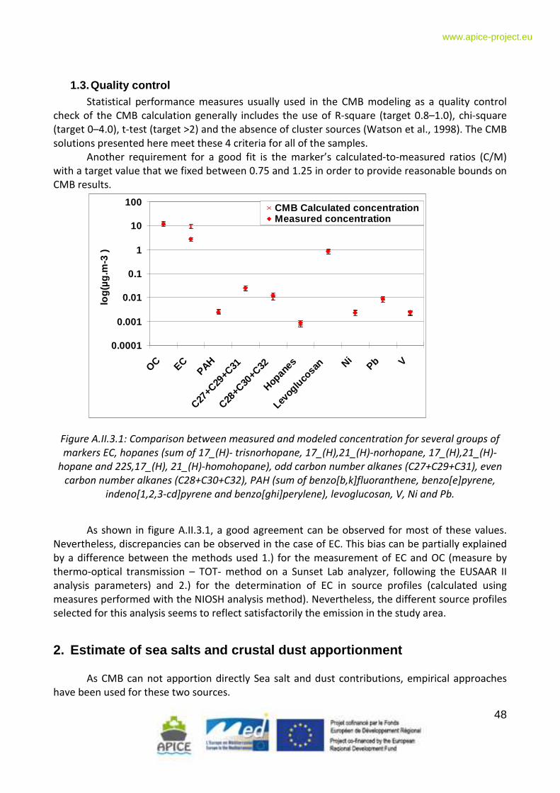
48


1.3. Quality control Statistical performance measures usually used in the CMB modeling as a quality control

check of the CMB calculation generally includes the use of R-square (target 0.8–1.0), chi-square

(target 0–4.0), t-test (target >2) and the absence of cluster sources (Watson et al., 1998). The CMB

solutions presented here meet these 4 criteria for all of the samples.

Another requirement for a good fit is the marker’s calculated-to-measured ratios (C/M)

with a target value that we fixed between 0.75 and 1.25 in order to provide reasonable bounds on

CMB results.

0.0001

0.001

0.01

0.1

1

10

100

OC ECPAH

C27+C

29+C

31

C28+C

30+C

32

Hopan

es

Levo

gluco

san Ni

Pb V

log(

µg.m

-3 )

CMB Calculated concentrationMeasured concentration

Figure A.II.3.1: Comparison between measured and modeled concentration for several groups of

markers EC, hopanes (sum of 17_(H)- trisnorhopane, 17_(H),21_(H)-norhopane, 17_(H),21_(H)-

hopane and 22S,17_(H), 21_(H)-homohopane), odd carbon number alkanes (C27+C29+C31), even

carbon number alkanes (C28+C30+C32), PAH (sum of benzo[b,k]fluoranthene, benzo[e]pyrene,

indeno[1,2,3-cd]pyrene and benzo[ghi]perylene), levoglucosan, V, Ni and Pb.

As shown in figure A.II.3.1, a good agreement can be observed for most of these values.

Nevertheless, discrepancies can be observed in the case of EC. This bias can be partially explained

by a difference between the methods used 1.) for the measurement of EC and OC (measure by

thermo-optical transmission – TOT- method on a Sunset Lab analyzer, following the EUSAAR II

analysis parameters) and 2.) for the determination of EC in source profiles (calculated using

measures performed with the NIOSH analysis method). Nevertheless, the different source profiles

selected for this analysis seems to reflect satisfactorily the emission in the study area.

2. Estimate of sea salts and crustal dust apportion ment

As CMB can not apportion directly Sea salt and dust contributions, empirical approaches

have been used for these two sources.

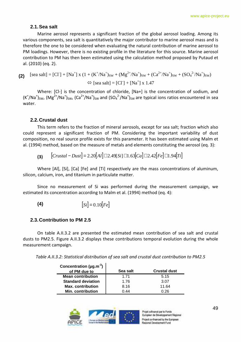
49


2.1. Sea salt Marine aerosol represents a significant fraction of the global aerosol loading. Among its

various components, sea salt is quantitatively the major contributor to marine aerosol mass and is

therefore the one to be considered when evaluating the natural contribution of marine aerosol to

PM loadings. However, there is no existing profile in the literature for this source. Marine aerosol

contribution to PM has then been estimated using the calculation method proposed by Putaud et

al. (2010) (eq. 2).

[sea salt] = [Cl-] + [Na+] x (1 + (K+/Na+)SW + (Mg2+/Na+)SW + (Ca2+/Na+)SW + (SO4

2-/Na+)SW)

� [sea salt] = [Cl-] + [Na+] x 1.47

Where: [Cl-] is the concentration of chloride, [Na+] is the concentration of sodium, and

(K+/Na

+)SW, (Mg

2+/Na

+)SW, (Ca

2+/Na

+)SW and (SO4

2-/Na

+)SW are typical ions ratios encountered in sea

water.

2.2. Crustal dust This term refers to the fraction of mineral aerosols, except for sea salt; fraction which also

could represent a significant fraction of PM. Considering the important variability of dust

composition, no real source profile exists for this parameter. It has been estimated using Malm et

al. (1994) method, based on the measure of metals and elements constituting the aerosol (eq. 3):

(3)

Where [Al], [Si], [Ca] [Fe] and [Ti] respectively are the mass concentrations of aluminum,

silicon, calcium, iron, and titanium in particulate matter.

Since no measurement of Si was performed during the measurement campaign, we

estimated its concentration according to Malm et al. (1994) method (eq. 4):

(4)

2.3. Contribution to PM 2.5

On table A.II.3.2 are presented the estimated mean contribution of sea salt and crustal

dusts to PM2.5. Figure A.II.3.2 displays these contributions temporal evolution during the whole

measurement campaign.

Table A.II.3.2: Statistical distribution of sea salt and crustal dust contribution to PM2.5

[ ] [ ] [ ] [ ] [ ]TiFeCaSiAlDustCrustal 94.142.263.1][49.220.2 ++++=−

[ ] [ ]FeSi 10.0=

(2)

Concentration (µg.m -3) of PM due to Sea salt Crustal dust

Mean contribution 1.71 5.15Standard deviation 1.76 3.07Max. contribution 8.16 11.64Min. contribution 0.44 0.26

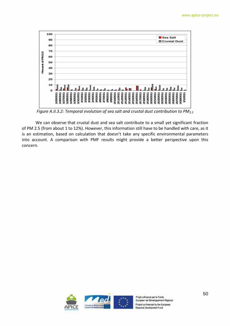
50


0

10

20

30

40

50

60

70

80

90

100

1/25

/201

11/

26/2

011

1/27

/201

11/

28/2

011

1/29

/201

11/

30/2

011

1/31

/201

12/

1/20

112/

2/20

112/

3/20

112/

4/20

112/

5/20

112/

6/20

112/

7/20

112/

8/20

112/

9/20

112/

10/2

011

2/11

/201

12/

12/2

011

2/13

/201

12/

14/2

011

2/15

/201

12/

16/2

011

2/17

/201

12/

18/2

011

2/19

/201

12/

20/2

011

2/21

/201

12/

22/2

011

2/23

/201

12/

24/2

011

2/25

/201

12/

26/2

011

2/27

/201

12/

28/2

011

3/1/

2011

Per

cent

of P

M 2

.5

Sea SaltCrustal Dust

Figure A.II.3.2: Temporal evolution of sea salt and crustal dust contribution to PM2.5

We can observe that crustal dust and sea salt contribute to a small yet significant fraction

of PM 2.5 (from about 1 to 12%). However, this information still have to be handled with care, as it

is an estimation, based on calculation that doesn’t take any specific environmental parameters

into account. A comparison with PMF results might provide a better perspective upon this

concern.

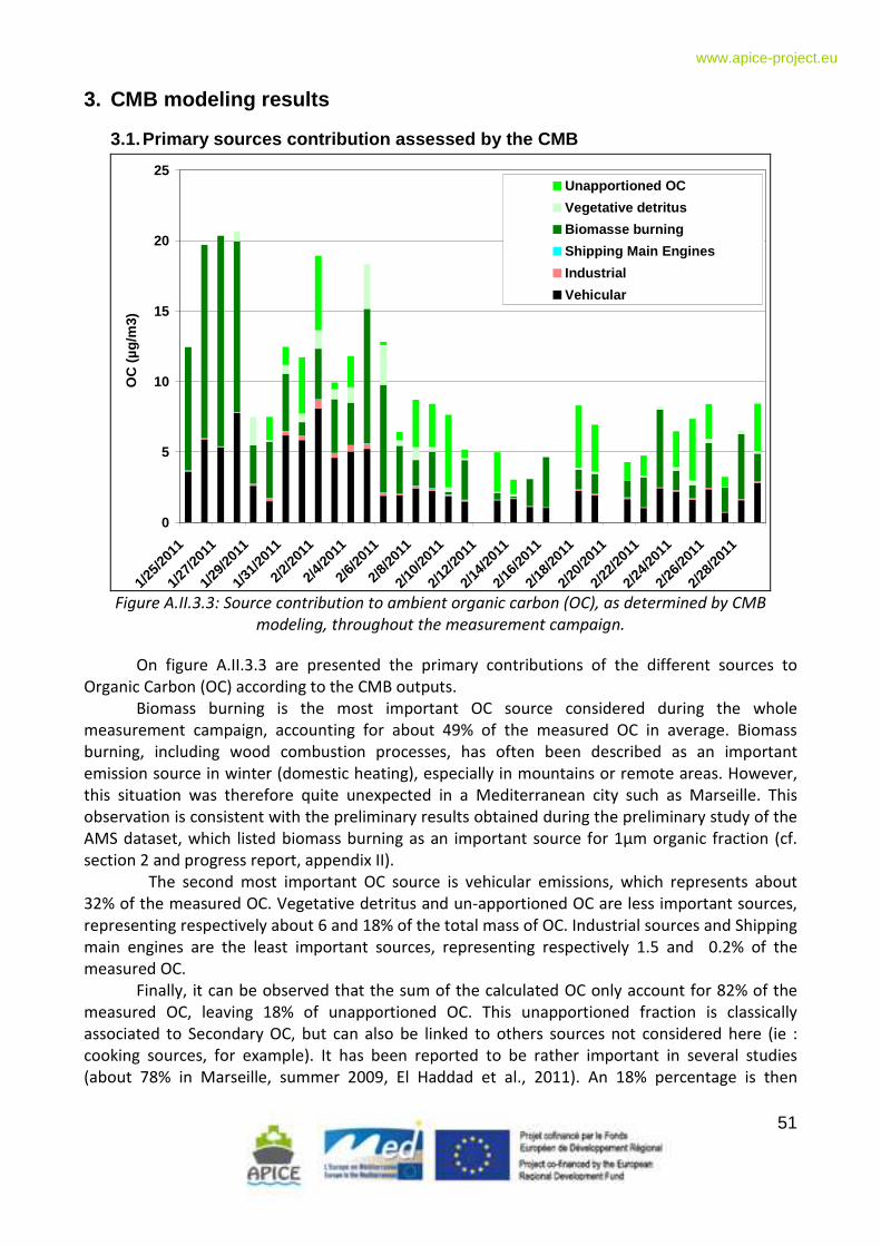
51


3. CMB modeling results

3.1. Primary sources contribution assessed by the C MB

0

5

10

15

20

25

1/25/

2011

1/27/

2011

1/29/

2011

1/31/

2011

2/2/2

011

2/4/2

011

2/6/2

011

2/8/2

011

2/10/

2011

2/12/

2011

2/14/

2011

2/16/

2011

2/18/

2011

2/20/

2011

2/22/

2011

2/24/

2011

2/26/

2011

2/28/

2011

OC

(µg

/m3)

Unapportioned OC

Vegetative detritus

Biomasse burning

Shipping Main Engines

Industrial

Vehicular

Figure A.II.3.3: Source contribution to ambient organic carbon (OC), as determined by CMB

modeling, throughout the measurement campaign.

On figure A.II.3.3 are presented the primary contributions of the different sources to

Organic Carbon (OC) according to the CMB outputs. Biomass burning is the most important OC source considered during the whole

measurement campaign, accounting for about 49% of the measured OC in average. Biomass

burning, including wood combustion processes, has often been described as an important

emission source in winter (domestic heating), especially in mountains or remote areas. However,

this situation was therefore quite unexpected in a Mediterranean city such as Marseille. This

observation is consistent with the preliminary results obtained during the preliminary study of the

AMS dataset, which listed biomass burning as an important source for 1µm organic fraction (cf.

section 2 and progress report, appendix II).

The second most important OC source is vehicular emissions, which represents about

32% of the measured OC. Vegetative detritus and un-apportioned OC are less important sources,

representing respectively about 6 and 18% of the total mass of OC. Industrial sources and Shipping

main engines are the least important sources, representing respectively 1.5 and 0.2% of the

measured OC.

Finally, it can be observed that the sum of the calculated OC only account for 82% of the

measured OC, leaving 18% of unapportioned OC. This unapportioned fraction is classically

associated to Secondary OC, but can also be linked to others sources not considered here (ie :

cooking sources, for example). It has been reported to be rather important in several studies

(about 78% in Marseille, summer 2009, El Haddad et al., 2011). An 18% percentage is then

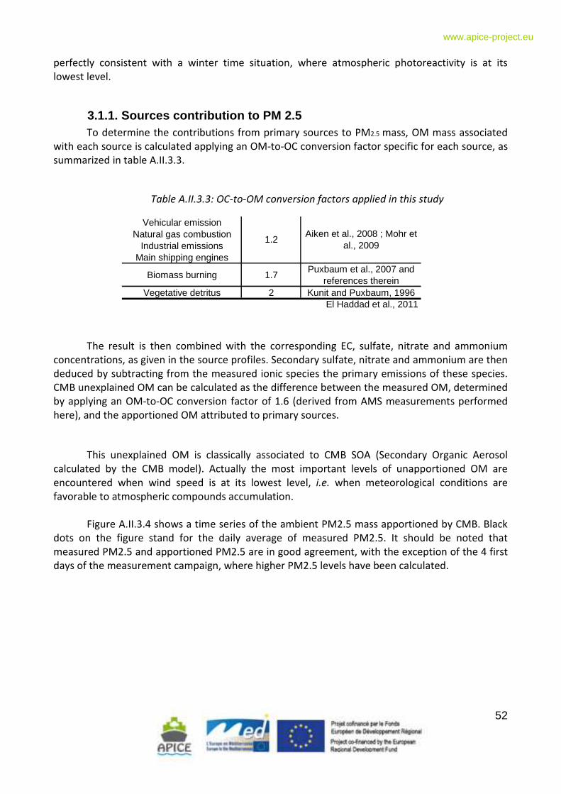
52


perfectly consistent with a winter time situation, where atmospheric photoreactivity is at its

lowest level.

3.1.1. Sources contribution to PM 2.5 To determine the contributions from primary sources to PM2.5 mass, OM mass associated

with each source is calculated applying an OM-to-OC conversion factor specific for each source, as

summarized in table A.II.3.3.

Table A.II.3.3: OC-to-OM conversion factors applied in this study

The result is then combined with the corresponding EC, sulfate, nitrate and ammonium

concentrations, as given in the source profiles. Secondary sulfate, nitrate and ammonium are then

deduced by subtracting from the measured ionic species the primary emissions of these species.

CMB unexplained OM can be calculated as the difference between the measured OM, determined

by applying an OM-to-OC conversion factor of 1.6 (derived from AMS measurements performed

here), and the apportioned OM attributed to primary sources.

This unexplained OM is classically associated to CMB SOA (Secondary Organic Aerosol

calculated by the CMB model). Actually the most important levels of unapportioned OM are

encountered when wind speed is at its lowest level, i.e. when meteorological conditions are

favorable to atmospheric compounds accumulation.

Figure A.II.3.4 shows a time series of the ambient PM2.5 mass apportioned by CMB. Black

dots on the figure stand for the daily average of measured PM2.5. It should be noted that

measured PM2.5 and apportioned PM2.5 are in good agreement, with the exception of the 4 first

days of the measurement campaign, where higher PM2.5 levels have been calculated.

Vehicular emissionNatural gas combustion

Industrial emissionsMain shipping engines

Biomass burning 1.7Puxbaum et al., 2007 and

references thereinVegetative detritus 2 Kunit and Puxbaum, 1996

1.2Aiken et al., 2008 ; Mohr et

al., 2009

El Haddad et al., 2011

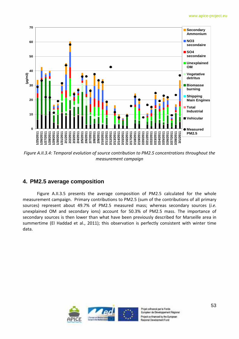
53


0

10

20

30

40

50

60

70

1/25

/201

11/

26/2

011

1/27

/201

11/

28/2

011

1/29

/201

11/

30/2

011

1/31

/201

12/

1/20

112/

2/20

112/

3/20

112/

4/20

112/

5/20

112/

6/20

112/

7/20

112/

8/20

112/

9/20

112/

10/2

011

2/11

/201

12/

12/2

011

2/13

/201

12/

14/2

011

2/15

/201

12/

16/2

011

2/17

/201

12/

18/2

011

2/19

/201

12/

20/2

011

2/21

/201

12/

22/2

011

2/23

/201

12/

24/2

011

2/25

/201

12/

26/2

011

2/27

/201

12/

28/2

011

3/1/

2011

(µg/

m3)

SecondaryAmmonium

NO3secondaire

SO4secondaire

UnexplainedOM

Vegetativedetritus

Biomasseburning

ShippingMain Engines

TotalIndustrial

Vehicular

MeasuredPM2.5

Figure A.II.3.4: Temporal evolution of source contribution to PM2.5 concentrations throughout the

measurement campaign

4. PM2.5 average composition

Figure A.II.3.5 presents the average composition of PM2.5 calculated for the whole

measurement campaign. Primary contributions to PM2.5 (sum of the contributions of all primary

sources) represent about 49.7% of PM2.5 measured mass; whereas secondary sources (i.e.

unexplained OM and secondary ions) account for 50.3% of PM2.5 mass. The importance of

secondary sources is then lower than what have been previously described for Marseille area in

summertime (El Haddad et al., 2011); this observation is perfectly consistent with winter time

data.

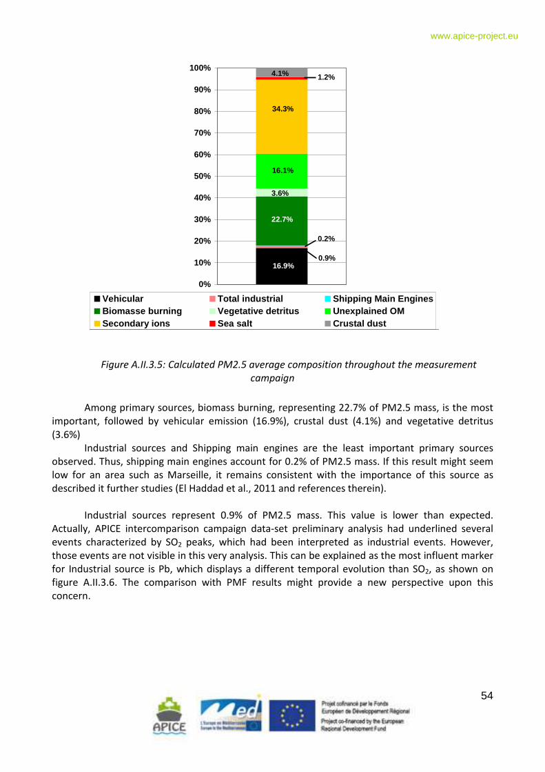
54


Figure A.II.3.5: Calculated PM2.5 average composition throughout the measurement

campaign

Among primary sources, biomass burning, representing 22.7% of PM2.5 mass, is the most

important, followed by vehicular emission (16.9%), crustal dust (4.1%) and vegetative detritus

(3.6%)

Industrial sources and Shipping main engines are the least important primary sources

observed. Thus, shipping main engines account for 0.2% of PM2.5 mass. If this result might seem

low for an area such as Marseille, it remains consistent with the importance of this source as

described it further studies (El Haddad et al., 2011 and references therein).

Industrial sources represent 0.9% of PM2.5 mass. This value is lower than expected.

Actually, APICE intercomparison campaign data-set preliminary analysis had underlined several

events characterized by SO2 peaks, which had been interpreted as industrial events. However,

those events are not visible in this very analysis. This can be explained as the most influent marker

for Industrial source is Pb, which displays a different temporal evolution than SO2, as shown on

figure A.II.3.6. The comparison with PMF results might provide a new perspective upon this

concern.

0%

10%

20%

30%

40%

50%

60%

70%

80%

90%

100%

Vehicular Total industrial Shipping Main EnginesBiomasse burning Vegetative detritus Unexplained OMSecondary ions Sea salt Crustal dust

34.3%

16.1%

4.1%

3.6%

22.7%

16.9%

1.2%

0.9%

0.2%

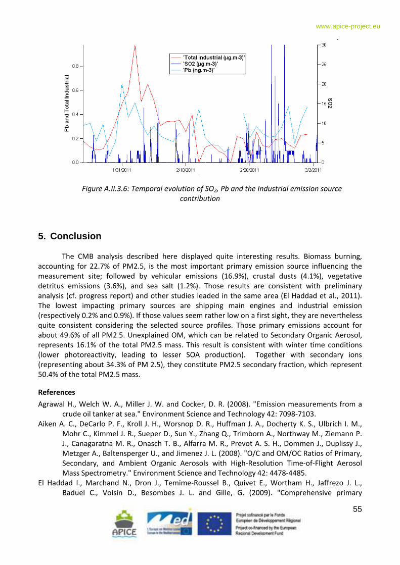
55


Figure A.II.3.6: Temporal evolution of SO2, Pb and the Industrial emission source

contribution

5. Conclusion

The CMB analysis described here displayed quite interesting results. Biomass burning,

accounting for 22.7% of PM2.5, is the most important primary emission source influencing the

measurement site; followed by vehicular emissions (16.9%), crustal dusts (4.1%), vegetative

detritus emissions (3.6%), and sea salt (1.2%). Those results are consistent with preliminary

analysis (cf. progress report) and other studies leaded in the same area (El Haddad et al., 2011).

The lowest impacting primary sources are shipping main engines and industrial emission

(respectively 0.2% and 0.9%). If those values seem rather low on a first sight, they are nevertheless

quite consistent considering the selected source profiles. Those primary emissions account for

about 49.6% of all PM2.5. Unexplained OM, which can be related to Secondary Organic Aerosol,

represents 16.1% of the total PM2.5 mass. This result is consistent with winter time conditions

(lower photoreactivity, leading to lesser SOA production). Together with secondary ions

(representing about 34.3% of PM 2.5), they constitute PM2.5 secondary fraction, which represent

50.4% of the total PM2.5 mass.

References

Agrawal H., Welch W. A., Miller J. W. and Cocker, D. R. (2008). "Emission measurements from a

crude oil tanker at sea." Environment Science and Technology 42: 7098-7103.

Aiken A. C., DeCarlo P. F., Kroll J. H., Worsnop D. R., Huffman J. A., Docherty K. S., Ulbrich I. M.,

Mohr C., Kimmel J. R., Sueper D., Sun Y., Zhang Q., Trimborn A., Northway M., Ziemann P.

J., Canagaratna M. R., Onasch T. B., Alfarra M. R., Prevot A. S. H., Dommen J., Duplissy J.,

Metzger A., Baltensperger U., and Jimenez J. L. (2008). "O/C and OM/OC Ratios of Primary,

Secondary, and Ambient Organic Aerosols with High-Resolution Time-of-Flight Aerosol

Mass Spectrometry." Environment Science and Technology 42: 4478-4485.

El Haddad I., Marchand N., Dron J., Temime-Roussel B., Quivet E., Wortham H., Jaffrezo J. L.,

Baduel C., Voisin D., Besombes J. L. and Gille, G. (2009). "Comprehensive primary

56


particulate organic characterization of vehicular exhaust emissions in France." Atmospheric

Environment 43: 6190-6198.

El Haddad I., Marchand N., Wortham H., Piot C., BesombesJ.-L., Cozic J., Chauvel C., Armengaud A.,

Robin D. and JaffrezoJ.-L. (2011). "Primary sources of PM2.5 organic aerosol in an industrial

Mediterranean city, Marseille." Atmospheric Chemistry and Physics 11: 2039-2058,.

Favez O., El Haddad I., Piot C., Boréave A., Abidi E., Marchand N., Jaffrezo J.-L., Besombes J.-L.,

Personnaz M.-B., Sciare J., Wortham H., George C. and D’Anna B. (2010). "Inter-comparison

of source apportionment models for the estimation of wood burning aerosols during

wintertime in an Alpine city (Grenoble, France),." Atmospheric Chemistry and Physics 10:

5295–5314.

Fine P. M., Cass G. R., and Simoneit B. R. T. (2002). "Chemical Characterization of Fine Particle

Emissions from the Fireplace Combustion of Woods Grown in the Southern United States."

Environment Science and Technology 36: 1442-1451.

Kunit M., and Puxbaum H. (1996). "Enzymatic determination of the cellulose content of

atmospheric aerosols." Atmospheric Environment 30: 1233-1236.

Malm W.C., Sisler J.F., Huffman D., Eldred R.A. and Cahill T.A., (1994). "Spatial and seasonal trends

in particle concentration and optical extinction in the United States." Journal of

Geophysical Research 99(D1): 1347-1370.

Mohr C., Huffman J. A., Cubison M. J., Aiken A. C., Docherty K. S., Kimmel J. R., Ulbrich I. M.,

Hannigan M. and Jimenez J. L. (2009). "Characterization of Primary Organic Aerosol

Emissions from Meat Cooking, Trash Burning, and Motor Vehicles with High-Resolution

Aerosol Mass Spectrometry and Comparison with Ambient and Chamber Observations."

Environment Science and Technology 43: 2443-2449.

Putaud J.P., Raes F., Van Dingenen R., Brüggemann E., Facchini M.C., Stefano Decesari S., Fuzzi S.,

Gehrig R., Hüglin C., Laj P., Lorbeer G., Maenhaut W., Mihalopoulos N., Müller K., Querol X.,

Rodriguez S., Schneider J., Spindler G., Brink H., Tørseth K. and Wiedensohler A. (2004). "A

European aerosol phenomenology e 3: Physical and chemical characteristics of particulate

matter from 60 rural, urban, and kerbside sites across Europe." Atmospheric Environment

38(16): 2579-2595.

Puxbaum H., Caseiro A., Sanchez-Ochoa A., Kasper-Giebl A., Claeys M., Gelencser A., Legrand M.,

Preunkert S. and Pio C. (2007). "Levoglucosan levels at background sites in Europe for

assessing the impact of biomass combustion on the European aerosol background." Journal

of Geophysical Research 112(D23S05).

Rogge W. F., Hildemann L. M., Mazurek M. A., Cass G. R. and Simoneit B. R. T. (1993(a)). "Sources

of Fine Organic Aerosol .4. Particulate Abrasion Products from Leaf Surfaces of Urban

Plants." Environment Science and Technology 27: 2700-2711.

Rogge W. F., Hildemann L. M., Mazurek M. A., Cass G. R., and Simoneit B. R. T. (1993(b)). " Sources

of Fine Organic Aerosol.5. Natural-Gas Home Appliances." Environment Science and

Technology 27: 2736-2744.

Tsai J.-H., L. K.-H., Chen C.-Y., Ding J.-Y., Choa C.-G., and Chiang H.-L. (2007). "Chemical

constituents in particulate emissions from an integrated iron and steel facility." Journal of

Hazardous Materials 147: 111-119.

Weitkamp E. A., Lipsky E. M., Pancras P. J., Ondov J. M., Polidori A., Turpin B. J., and Robinson A. L.

(2005). "Fine particle emission profile for a large coke production facility based on highly

time-resolved fence line measurements." Atmospheric Environment 39: 6719-6733.

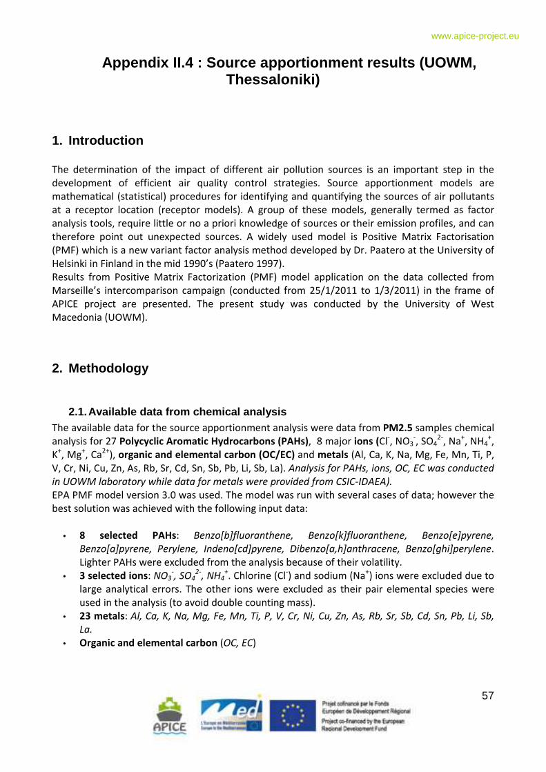
57


Appendix II.4 : Source apportionment results (UOWM, Thessaloniki)

1. Introduction

The determination of the impact of different air pollution sources is an important step in the

development of efficient air quality control strategies. Source apportionment models are

mathematical (statistical) procedures for identifying and quantifying the sources of air pollutants

at a receptor location (receptor models). A group of these models, generally termed as factor

analysis tools, require little or no a priori knowledge of sources or their emission profiles, and can

therefore point out unexpected sources. A widely used model is Positive Matrix Factorisation

(PMF) which is a new variant factor analysis method developed by Dr. Paatero at the University of

Helsinki in Finland in the mid 1990’s (Paatero 1997).

Results from Positive Matrix Factorization (PMF) model application on the data collected from

Marseille’s intercomparison campaign (conducted from 25/1/2011 to 1/3/2011) in the frame of

APICE project are presented. The present study was conducted by the University of West

Macedonia (UOWM).

2. Methodology

2.1. Available data from chemical analysis The available data for the source apportionment analysis were data from PM2.5 samples chemical

analysis for 27 Polycyclic Aromatic Hydrocarbons (PAHs), 8 major ions (Cl-, NO3

-, SO4

2-, Na

+, NH4

+,

K+, Mg

+, Ca

2+), organic and elemental carbon (OC/EC) and metals (Al, Ca, K, Na, Mg, Fe, Mn, Ti, P,

V, Cr, Ni, Cu, Zn, As, Rb, Sr, Cd, Sn, Sb, Pb, Li, Sb, La). Analysis for PAHs, ions, OC, EC was conducted

in UOWM laboratory while data for metals were provided from CSIC-IDAEA).

EPA PMF model version 3.0 was used. The model was run with several cases of data; however the

best solution was achieved with the following input data:

• 8 selected PAHs: Benzo[b]fluoranthene, Benzo[k]fluoranthene, Benzo[e]pyrene,

Benzo[a]pyrene, Perylene, Indeno[cd]pyrene, Dibenzo[a,h]anthracene, Benzo[ghi]perylene.

Lighter PAHs were excluded from the analysis because of their volatility.

• 3 selected ions: NO3-, SO4

2-, NH4

+. Chlorine (Cl

-) and sodium (Na

+) ions were excluded due to

large analytical errors. The other ions were excluded as their pair elemental species were

used in the analysis (to avoid double counting mass).

• 23 metals: Al, Ca, K, Na, Mg, Fe, Mn, Ti, P, V, Cr, Ni, Cu, Zn, As, Rb, Sr, Sb, Cd, Sn, Pb, Li, Sb,

La.

• Organic and elemental carbon (OC, EC)

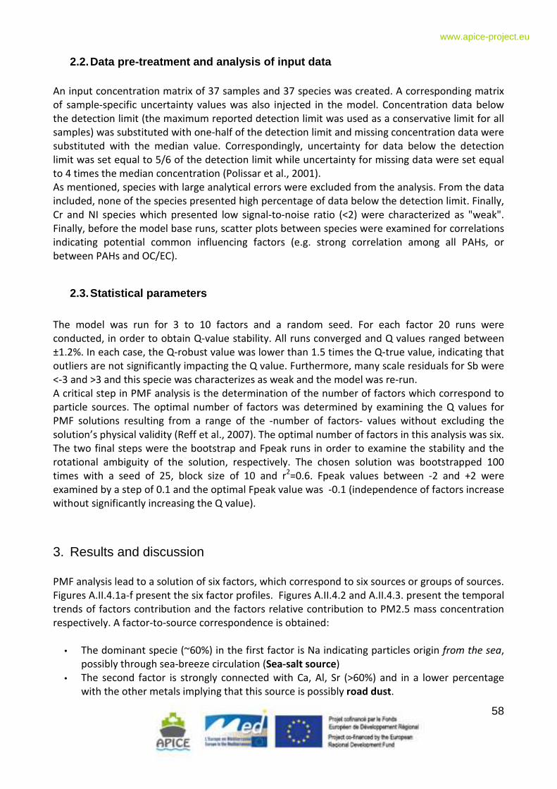
58


2.2. Data pre-treatment and analysis of input data An input concentration matrix of 37 samples and 37 species was created. A corresponding matrix

of sample-specific uncertainty values was also injected in the model. Concentration data below

the detection limit (the maximum reported detection limit was used as a conservative limit for all

samples) was substituted with one-half of the detection limit and missing concentration data were

substituted with the median value. Correspondingly, uncertainty for data below the detection

limit was set equal to 5/6 of the detection limit while uncertainty for missing data were set equal

to 4 times the median concentration (Polissar et al., 2001).

As mentioned, species with large analytical errors were excluded from the analysis. From the data

included, none of the species presented high percentage of data below the detection limit. Finally,

Cr and NI species which presented low signal-to-noise ratio (<2) were characterized as "weak".

Finally, before the model base runs, scatter plots between species were examined for correlations

indicating potential common influencing factors (e.g. strong correlation among all PAHs, or

between PAHs and OC/EC).

2.3. Statistical parameters

The model was run for 3 to 10 factors and a random seed. For each factor 20 runs were

conducted, in order to obtain Q-value stability. All runs converged and Q values ranged between

±1.2%. In each case, the Q-robust value was lower than 1.5 times the Q-true value, indicating that

outliers are not significantly impacting the Q value. Furthermore, many scale residuals for Sb were

<-3 and >3 and this specie was characterizes as weak and the model was re-run.

A critical step in PMF analysis is the determination of the number of factors which correspond to

particle sources. The optimal number of factors was determined by examining the Q values for

PMF solutions resulting from a range of the -number of factors- values without excluding the

solution’s physical validity (Reff et al., 2007). The optimal number of factors in this analysis was six.

The two final steps were the bootstrap and Fpeak runs in order to examine the stability and the

rotational ambiguity of the solution, respectively. The chosen solution was bootstrapped 100

times with a seed of 25, block size of 10 and r2=0.6. Fpeak values between -2 and +2 were

examined by a step of 0.1 and the optimal Fpeak value was -0.1 (independence of factors increase

without significantly increasing the Q value).

3. Results and discussion

PMF analysis lead to a solution of six factors, which correspond to six sources or groups of sources.

Figures A.II.4.1a-f present the six factor profiles. Figures A.II.4.2 and A.II.4.3. present the temporal

trends of factors contribution and the factors relative contribution to PM2.5 mass concentration

respectively. A factor-to-source correspondence is obtained:

• The dominant specie (~60%) in the first factor is Na indicating particles origin from the sea,

possibly through sea-breeze circulation (Sea-salt source)

• The second factor is strongly connected with Ca, Al, Sr (>60%) and in a lower percentage

with the other metals implying that this source is possibly road dust.

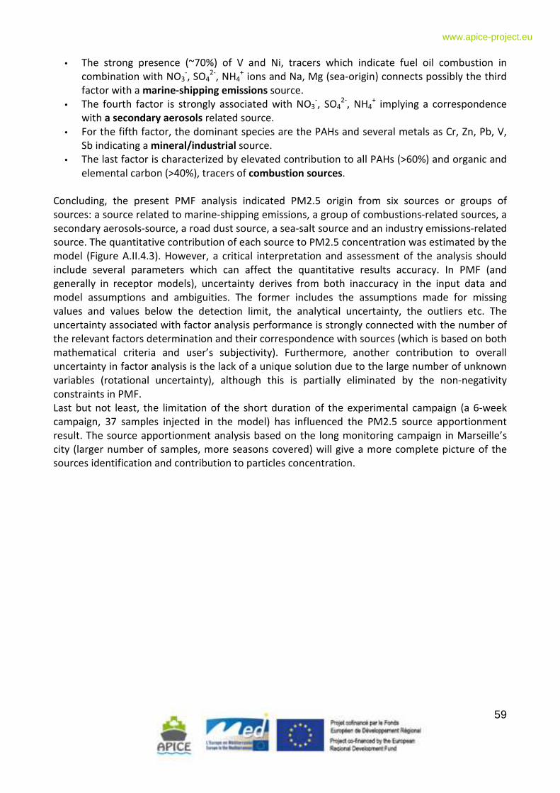
59


• The strong presence (~70%) of V and Ni, tracers which indicate fuel oil combustion in

combination with NO3-, SO4

2-, NH4

+ ions and Na, Mg (sea-origin) connects possibly the third

factor with a marine-shipping emissions source.

• The fourth factor is strongly associated with NO3-, SO4

2-, NH4

+ implying a correspondence

with a secondary aerosols related source.

• For the fifth factor, the dominant species are the PAHs and several metals as Cr, Zn, Pb, V,

Sb indicating a mineral/industrial source.

• The last factor is characterized by elevated contribution to all PAHs (>60%) and organic and

elemental carbon (>40%), tracers of combustion sources.

Concluding, the present PMF analysis indicated PM2.5 origin from six sources or groups of

sources: a source related to marine-shipping emissions, a group of combustions-related sources, a

secondary aerosols-source, a road dust source, a sea-salt source and an industry emissions-related

source. The quantitative contribution of each source to PM2.5 concentration was estimated by the

model (Figure A.II.4.3). However, a critical interpretation and assessment of the analysis should

include several parameters which can affect the quantitative results accuracy. In PMF (and

generally in receptor models), uncertainty derives from both inaccuracy in the input data and

model assumptions and ambiguities. The former includes the assumptions made for missing

values and values below the detection limit, the analytical uncertainty, the outliers etc. The

uncertainty associated with factor analysis performance is strongly connected with the number of

the relevant factors determination and their correspondence with sources (which is based on both

mathematical criteria and user’s subjectivity). Furthermore, another contribution to overall

uncertainty in factor analysis is the lack of a unique solution due to the large number of unknown

variables (rotational uncertainty), although this is partially eliminated by the non-negativity

constraints in PMF.

Last but not least, the limitation of the short duration of the experimental campaign (a 6-week

campaign, 37 samples injected in the model) has influenced the PM2.5 source apportionment

result. The source apportionment analysis based on the long monitoring campaign in Marseille’s

city (larger number of samples, more seasons covered) will give a more complete picture of the

sources identification and contribution to particles concentration.

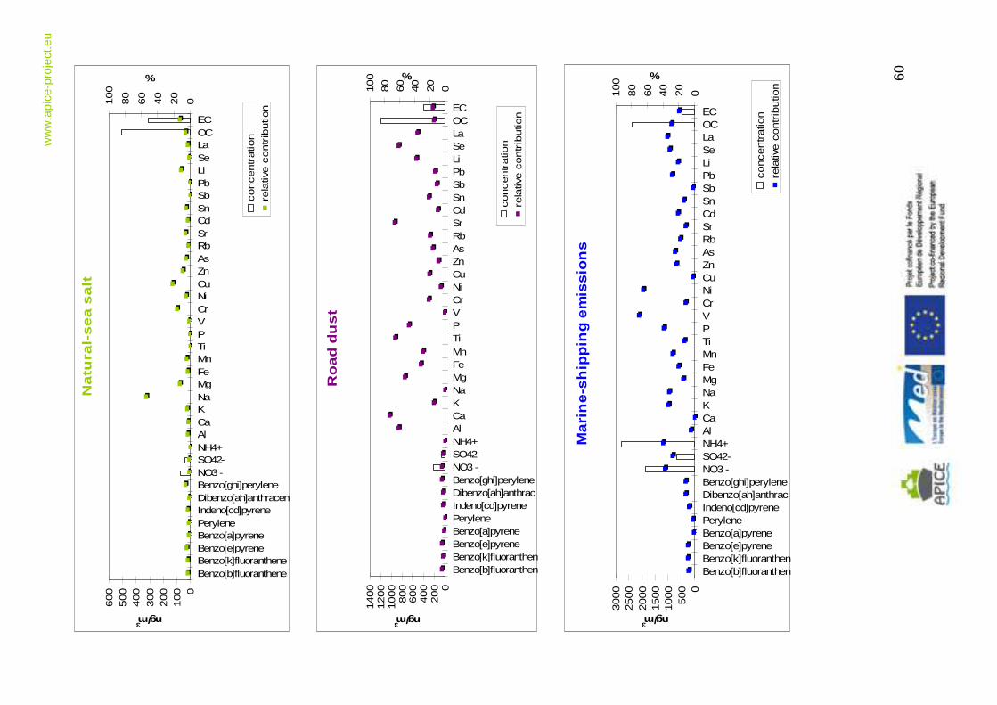
60

ww

w.a

pice

-pro

ject

.eu

Na

tura

l-se

a s

alt

0100

200

300

400

500

600

Benzo[b]fluorantheneBenzo[k]fluorantheneBenzo[e]pyreneBenzo[a]pyrenePeryleneIndeno[cd]pyreneDibenzo[ah]anthracenBenzo[ghi]peryleneNO3 -SO42-NH4+AlCaKNaMgFeMnTiPV Cr Ni Cu Zn As Rb Sr Cd Sn Sb Pb Li SeLaOC ΕC

ng/m3

020

40

60

80

100

%

concentr

ation

rela

tive c

ontr

ibution

Roa

d d

ust

0200

400

600

800

1000

1200

1400

Benzo[b]fluoranthenBenzo[k]fluoranthenBenzo[e]pyreneBenzo[a]pyrenePeryleneIndeno[cd]pyreneDibenzo[ah]anthracBenzo[ghi]peryleneNO3 -SO42-NH4+AlCaKNaMgFeMnTiPV Cr Ni Cu Zn As Rb Sr Cd Sn Sb Pb Li SeLaOC ΕC

ng/m3

020

40

60

80

100

%

concentr

atio

nre

lativ

e c

ontr

ibutio

n

Ma

rin

e-s

hip

pin

g e

mis

sion

s

0500

1000

1500

2000

2500

3000


ng/m3

020

40

60

80

100

%

concentr

atio

n

rela

tive c

ontr

ibutio

n

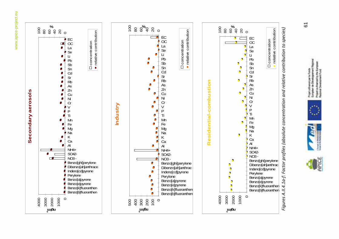
61

ww

w.a

pice

-pro

ject

.eu

Se

co

nda

ry a

ero

sols

0

1000

2000

3000

4000

Benzo[b]fluoranthenBenzo[k]fluoranthenBenzo[e]pyreneBenzo[a]pyrenePeryleneIndeno[cd]pyreneDibenzo[ah]anthraceBenzo[ghi]peryleneNO3 -SO42-NH4+AlCaKNaMgFeMnTiPV Cr Ni Cu Zn As Rb Sr Cd Sn Sb Pb Li SeLaOC ΕC

ng/m3

020

40

60

80

100

%

concentr

ation

rela

tive

contr

ibution

Ind

ustr

y

0

100

200

300

400

500


ng/m3

020

40

60

80

100 %

concentr

atio

n

rela

tive c

ontr

ibutio

n

Re

sid

en

tia

l-com

bu

stion

0

1000

2000

3000

4000


ng/m3

020

40

60

80

100

%

concentr

ation

rela

tive

contr

ibution

F

igu

res

A.I

I.4

.1a

-f:

Fa

cto

r p

rofi

les

(ab

solu

te c

on

cen

tra

tio

n a

nd

re

lati

ve

co

ntr

ibu

tio

n t

o s

pe

cie

s)

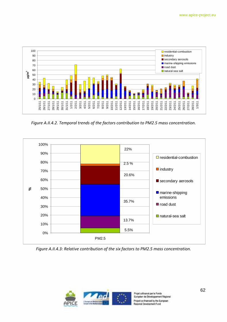
62


0

10

20

30

40

50

60

70

80

90

100

25/1

/11

26/1

/11

27/1

/11

28/1

/11

29/1

/11

30/1

/11

31/1

/11

1/2/

11

2/2/

11

3/2/

11

4/2/

11

5/2/

11

6/2/

11

7/2/

11

8/2/

11

9/2/

11

10/2

/11

11/2

/11

12/2

/11

13/2

/11

14/2

/11

15/2

/11

16/2

/11

17/2

/11

18/2

/11

19/2

/11

20/2

/11

21/2

/11

22/2

/11

23/2

/11

24/2

/11

25/2

/11

26/2

/11

27/2

/11

28/2

/11

1/3/

11

µg/

m3

residential-combustionindustrysecondary aerosolsmarine-shipping emissionsroad dustnatural-sea salt

Figure A.II.4.2. Temporal trends of the factors contribution to PM2.5 mass concentration.

5.5%

13.7%

35.7%

20.6%

2.5 %

22%

0%

10%

20%

30%

40%

50%

60%

70%

80%

90%

100%

PM2.5

%

residential-combustion

industry

secondary aerosols

marine-shippingemissions

road dust

natural-sea salt

Figure A.II.4.3: Relative contribution of the six factors to PM2.5 mass concentration.

63


Acknowledgements

The scientific team of University of West Macedonia would like to express acknowledgments to

CSIC-IDAEA group (especially to Jorge Pey and Noemi Perez) for the provided filters for chemical

analysis and data from metals analysis.

References

Cao Q., Wang H., Chen G.(2011). Source Apportionment of PAHs Using Two Mathematical Models

for Mangrove Sediments in Shantou Coastal Zone, China, Estuaries and Coasts, Volume 34,

Issue 5, September 2011, p.p. 950-960

Paatero P (1997). Least squares formulation of robust non-negative factor analysis. Chemometr.

Intelligent Lab. Syst. 6037: 23-35

Polissar A.V, Hopke P.K., and Poitrot R.L. (2001). Atmospheric aerosol over Vermont: chemical

composition and sources. Environ. Sci. Technol. 35 (23), 4604-4621.

Reff A., Eberly S., Bhave P. (2007). Receptor Modeling of ambient particulate matter data using

Positive Matrix Factorization: review of existing methods. J. Air & Waste Manage. Assoc.

57:146-154.

Vestenius, M., Leppänen, S., Anttila, P., Kyllönen, K., Hatakka, J., Hellén, H., Hyvärinen, A.-P.,

Hakola, H. (2011) Background concentrations and source apportionment of polycyclic

aromatic hydrocarbons in south-eastern Finland, Atmospheric Environment 45 (20), pp.

3391-3399

Wang, D., Tian, F., Yang, M., Liu, C., (2009). Application of positive matrix factorization to identify

potential sources of PAHs in soil of Dalian, China Environmental Pollution 157 (5), pp. 1559-

1564

64


Appendix II.5 : Source apportionment results (IDAEA -CSIC/U. Genoa, Venice)

1. Source apportionment approach

The source apportionment approach used by IDAEA group is PMF2 (Positive Matrix

Factorization, version 2), an advanced receptor model, developed by Paatero (Paatero et al, 1994)

that in the last years has been asserted to international level like most reliable. It is useful,

especially, where detailed data do not exist on the composition of the main emission sources, but

where large numbers of sampled data are available on ambient concentrations. The important

advantage of the positive matrix factorization is the ability to handle missing data and values

below the detection limits data by adjusting the error estimates of each data point. In fact, the

solution to the PMF problem depends on the uncertainties attributed to each value.

The errors associated to concentrations values were treated according to the procedure described

by Amato et al. (2009) and Escrig et al. (2009).

Mass apportionment was calculated performing a linear regression between the temporal

trends of sources resolved by PMF (Ramadan et al., 2000).

Among the output of the model, important parameters to consider are the explained

variations (EV). They indicate to what extent a source explains the temporal trend of an element.

The higher is the EV of an element in a source, the more this element is specifically “contained” in

that source if compared to the others. This, high EV for an element in a source identify that

element as a good tracer for the source. EV are a good help to associate factors with real chemical

– physical processes that emitted PM.

In the presented PMF analysis, PM measured components included elements, ions, organic

and elemental carbon measured by IDAEA group and and targeted sum of the organic species

described in Appendix 1: Even Alkanes (E-ALK: n-C(26-28-30-32)), Odd Alkanes (O-ALK: n-C(27-29-

31-33)), Heavy PAH (H-PAH: Benzo(b)fluoranthene, Benzo(j+k)fluoranthene, Benzo(a)pyrene,

Indeno(123-cd)pyrene, Dibenz(a,h)anthracene, Benzo(ghi)perylene), Hopanes (HOPA: 17alpha(H)-

22,29,30-Trisnorhopane, 17alpha(H),21beta(H)-30-Norhopane, 17alpha(H),21beta(H)-Hopane,

17alpha(H),21beta(H)-22S-Homohopane, 17alpha(H),21beta(H)-22R-Homohopane) and DeHydro

Abietic Acid (DHAA) measured by ARPAV.


2003) and 21 variables were finally used in the analysis: Ca, Na, Mg, Fe, SO42-

, V, Ni, Cu, Zn, Sn, Sb,

Pb, NO3-, NH4

+, EC, OC, E-ALK, O-ALK, H-PAH, HOPA, DHAA.

2. Results

Seven sources were resolved and labeled, according to their characteristic tracers, as

follows: Dust (traced by Ca), Road (divided into Vehicular exhaust + Sea Spray (traced by Cu, Zn, EC

and Na) and Road Dust (traced by Sb and Sn), Industrial/Marine (Oil Combustion, traced by V, Ni),

Secondary Compound divided into Secondary I (traced by SO42-

) and Secondary II (traced by NO3)

and Residential (Biomass Burning, traced by DHAA). PMF applied to a time series of elemental

concentration values resolved, over the number, the profiles (Figure AII.5.1) of PM sources at the

sampling site and their contribution to PM2.5 levels (Figure AII.5.2).

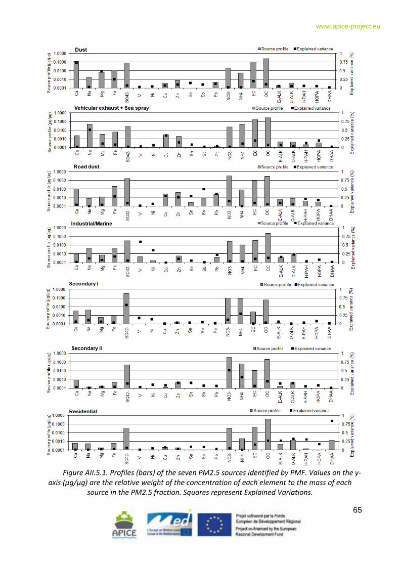
65


Figure AII.5.1. Profiles (bars) of the seven PM2.5 sources identified by PMF. Values on the y-

axis (µg/µg) are the relative weight of the concentration of each element to the mass of each

source in the PM2.5 fraction. Squares represent Explained Variations.

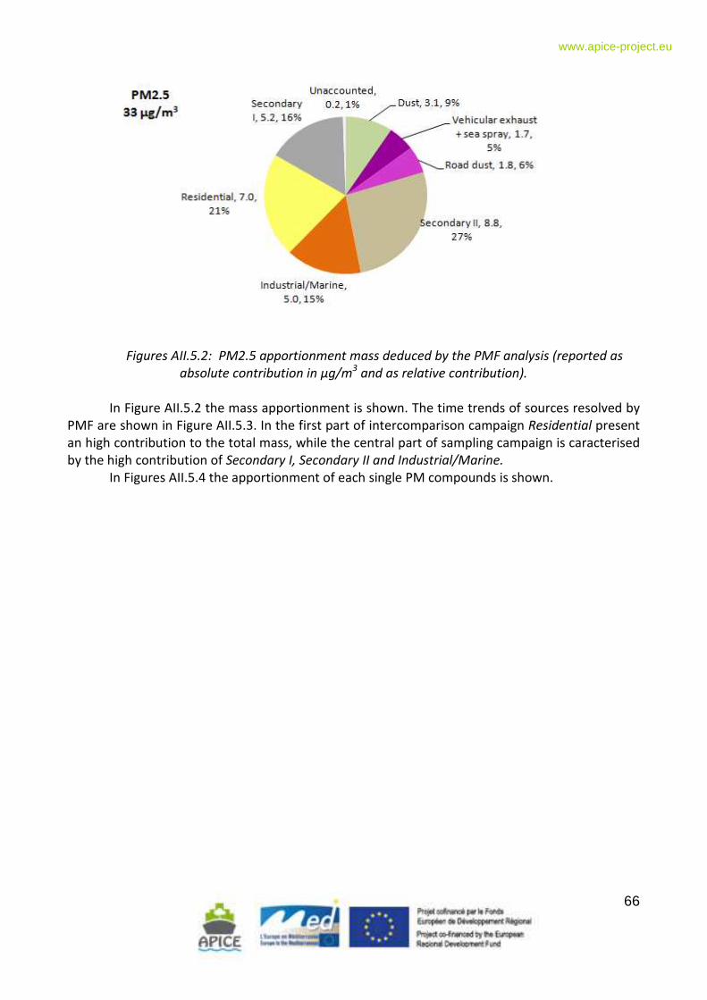
66


Figures AII.5.2: PM2.5 apportionment mass deduced by the PMF analysis (reported as

absolute contribution in µg/m3 and as relative contribution).

In Figure AII.5.2 the mass apportionment is shown. The time trends of sources resolved by

PMF are shown in Figure AII.5.3. In the first part of intercomparison campaign Residential present

an high contribution to the total mass, while the central part of sampling campaign is caracterised

by the high contribution of Secondary I, Secondary II and Industrial/Marine.

In Figures AII.5.4 the apportionment of each single PM compounds is shown.

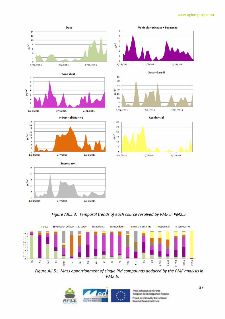
67


Figure AII.5.3: Temporal trends of each source resolved by PMF in PM2.5.

Figure AII.5.: Mass apportionment of single PM compounds deduced by the PMF analysis in

PM2.5.

final report intercomparison campaign final version

Documents