final report sub-saharan africa refinery project health study: volume i-a health...
TRANSCRIPT

Table of Contents
1
282828282828282828
Submitted by: ICF International
33 Hayden Avenue Lexington, MA USA Tel: 1 781 676 4000 Fax: 1.781 676 4005
& Lisa Robinson,
Independent Consultant & James Hammitt,
Harvard School of Public Health Valuation Subcontractors
Final Report Sub-Saharan Africa Refinery Project Health Study: Volume I-A Health Study June 2009 Submitted to: The World Bank and The African Refiners Association


3
World Bank
Volume I-A: Health Study Final Report
June, 2009
Prepared for: The World Bank and
The African Refiners Association
Prepared by: ICF International
33 Hayden Avenue Lexington, MA 02421
781 676 4000 with Lisa Robinson and James Hammitt,
Valuation Subcontractors

4
blankpageblankpage

Volume I-A: Health Study Final Report Table of Contents
ICF International World Bank June 2009
Table of Contents Health Study: Volume I-A 1. Purpose of the Health Study ..................................................................................................... 1-12. Overview of Health Study ......................................................................................................... 2-13. Emissions and Air Modeling ..................................................................................................... 3-1
3.1 Selection of Analysis Locations ....................................................................................... 3-13.2 Modeling Scenarios ...................................................................................................... 3-33.3 Pollutants and Averaging Periods ..................................................................................... 3-53.4 Air Quality Model ......................................................................................................... 3-6
3.4.1 Development of Emission Inventories ................................................................ 3-63.4.2 Geophysical Data (Land-Use and Terrain Elevation) ............................................. 3-93.4.3 Meteorological Data and Modeling .................................................................. 3-103.4.4 CALPUFF Modeling .................................................................................... 3-10
3.5 Regional Analyses ..................................................................................................... 3-103.5.1 Eastern Region .......................................................................................... 3-103.5.2 Western Region ......................................................................................... 3-243.5.3 Southern Region ........................................................................................ 3-41
3.6 Uncertainties Associated with the Air Modeling .................................................................. 3-583.6.1 Kampala, Uganda ....................................................................................... 3-583.6.2 Cotonou, Benin .......................................................................................... 3-593.6.3 Johannesburg, RSA .................................................................................... 3-593.6.4 Alternate Assumptions for Base Case Emissions Inventory .................................. 3-59
4. Health Impact Assessment ....................................................................................................... 4-14.1 Health Endpoints Associated with Key Air Pollutants ............................................................. 4-1
4.1.1 Determine Health Endpoints ............................................................................ 4-14.1.2 Health Endpoints Not Selected ........................................................................ 4-3
4.2 Selection of Health Studies ............................................................................................. 4-44.2.1 Initial Screening of Health Studies .................................................................... 4-44.2.2 Exposure-Response Functions ........................................................................ 4-54.2.3 Summary of Selected Studies .......................................................................... 4-6
4.3 Air Pollution/Health Studies from Sub-Saharan Africa ............................................................ 4-84.4 Compilation of Health Study Parameters ............................................................................ 4-9
4.4.1 Concentrations Used in the Health Assessment ................................................... 4-94.4.2 Compilation of Baseline Health Statistics ............................................................ 4-9
4.5 Uncertainties Associated with the Health Impact Assessment ............................................... 4-125. Health Valuation ...................................................................................................................... 5-1
5.1 Valuation Approaches ................................................................................................... 5-15.2 Mortality Risk Reductions ............................................................................................... 5-2

Volume I-A: Health Study Final Report Table of Contents
ICF International World Bank June 2009
5.2.1 VSL Literature Review ................................................................................... 5-35.2.2 VSL Recommendations ................................................................................. 5-45.2.3 Selected Values for Mortality Risk Valuations ...................................................... 5-5
5.3 Morbidity Risk Reductions .............................................................................................. 5-55.3.1 Chronic Bronchitis ........................................................................................ 5-65.3.2 Asthma Exacerbations ................................................................................... 5-65.3.3 Selected Values for Morbidity Risk Valuations ..................................................... 5-6
5.4 Uncertainties Associated with the Health Valuation ............................................................... 5-76. Calculation of Health Impacts and Monetary Benefits .................................................................... 6-1
6.1 East Region ................................................................................................................ 6-16.1.1 Quantitative City Evaluation - East Region .......................................................... 6-16.1.2 Qualitative City Evaluations - East Region .......................................................... 6-26.1.3 Regional Analysis - East Region ...................................................................... 6-2
6.2 West Region ............................................................................................................... 6-36.2.1 Quantitative City Evaluation - West SSA Region .................................................. 6-36.2.2 Qualitative City Evaluations - West SSA Region ................................................... 6-46.2.3 Regional Analysis - West SSA Region ............................................................... 6-4
6.3 South SSA Region ....................................................................................................... 6-56.3.1 Quantitative City Evaluation - South SSA Region .................................................. 6-56.3.2 Qualitative City Assessment - South SSA Region ................................................. 6-56.3.3 Regional Analysis - South SSA Region .............................................................. 6-6
6.4 Summary of Study Uncertainties ...................................................................................... 6-67. Health Study Summary and Discussion ...................................................................................... 7-18. References ............................................................................................................................. 8-1

Volume I-A: Health Study Final Report Table of Contents
ICF International World Bank June 2009
List of Tables Table 3-1: Cities Selected for Analysis ............................................................................................... 3-2Table 3-2: AFRI-4 Standards for Sulfur and Benzene Content in Fuel ........................................................ 3-4Table 3-3: Vehicle Activity Percentages for Different Vehicle Types in Kampala ......................................... 3-11Table 3-4: Summary of Total Emissions in Base Case Inventory for Kampala, Uganda ................................ 3-14Table 3-5: Summary of Total Emissions in Scenario 1 Inventory for Kampala, Uganda ................................ 3-15Table 3-6: Summary of Total Emissions in Scenario 2 Inventory for Kampala, Uganda ................................ 3-15Table 3-7: Base Case Modeling Results for Kampala, Uganda .............................................................. 3-16Table 3-8: Scenario 1 (AFRI-4 Fuel Specifications) Modeling Results for Kampala, Uganda ......................... 3-16Table 3-9: Scenario 2 (AFRI-4 Fuel Specifications with Control Technologies) Modeling Results for Kampala, Uganda ........................................................................................... 3-16Table 3-10: Modeled Annual Average (Spatially Averaged) Air Contaminant Concentrations in Densely Populated Areas - Kampala ............................................................................................... 3-17Table 3-11: Alternate Assumptions: Modeled Annual Average (Spatially Averaged) Air Contaminant Concentrations in Densely Populated Areas - Kampala .................................................. 3-17Table 3-12: Air Pollution Emission Summary for Nairobi, Kenya ............................................................. 3-18Table 3-13: Estimated Emissions for Dar Es Salaam City, Tanzania for Industry and Other Sources ............... 3-20Table 3-14: Qualitative Assessment for the Eastern SSA Region (Based on Comparison with Kampala) .......... 3-22Table 3-15: Vehicle Activity Percentages for Different Vehicle Types in Cotonou ....................................... 3-25Table 3-16. Shares of Modes of Transport in Use in 14 African Cities ...................................................... 3-27Table 3-17: Summary of Total Emissions in Base Case Inventory for Cotonou, Benin .................................. 3-30Table 3-18: Summary of Total Emissions in Scenario 1 Inventory for Cotonou, Benin .................................. 3-30Table 3-19: Summary of Total Emissions in Scenario 2 Inventory for Cotonou, Benin .................................. 3-31Table 3-20: Base Case Modeling Results for Cotonou ......................................................................... 3-32Table 3-21: Scenario 1 Modeling Results (AFRI-4 Fuel Specifications) for Cotonou .................................... 3-33Table 3-22: Scenario 2 Modeling Results (AFRI-4 Fuel Specifications with Control Technologies) for Cotonou .. 3-33Table 3-23: Modeled Annual Average (Spatially Averaged) Air Contaminant Concentrations in Densely Populated Areas - Cotonou ............................................................................................... 3-34Table 3-24: Alternate Assumptions: Modeled Annual Average (Spatially Averaged) Total PM Concentrations in Densely Population Areas - Cotonou ........................................................... 3-34Table 3-25: Citywide Base Case Emissions by Source Category in Ouagadougou, Burkina Faso ................... 3-36Table 3-26: Citywide Scenario 1 Emissions by Source Category in Ouagadougou, Burkina Faso ................... 3-36Table 3-27: Citywide Base Case Emissions by Source Category in Lagos, Nigeria ..................................... 3-37Table 3-28: Citywide Scenario 1 Emissions by Source Category in Lagos, Nigeria ...................................... 3-37Table 3-29: Qualitative Assessment for the West SSA Region (Based on Comparison with Cotonou) .............. 3-39Table 3-30: Summary of Total Emissions in Base Case Inventory for Johannesburg, South Africa .................. 3-45Table 3-31: Summary of Total Emissions in Scenario 1 Inventory for Johannesburg, South Africa .................. 3-46Table 3-32: Summary of Total Emissions in Scenario 2 Inventory for Johannesburg, South Africa .................. 3-46Table 3-33: Monitoring Data for Johannesburg Air Quality, for Evaluation of Model Output ........................... 3-48

Volume I-A: Health Study Final Report Table of Contents
ICF International World Bank June 2009
Table 3-34: Base Case CALPUFF Modeling Results for Johannesburg .................................................... 3-49Table 3-35: Scenario 1 (AFRI-4 Fuel Specifications) Modeling Results for Johannesburg ........................... 3-49Table 3-36: Scenario 2 (AFRI-4 Fuel Specifications With Control Technologies) Modeling Results for Johannesburg ................................................................................................ 3-49Table 3-37: Modeled Annual Average (Spatially Averaged) Air Contaminant Concentrations in Densely Populated Areas for Johannesburg ...................................................................................... 3-50Table 3-38: Vehicle Counts for Cape Town from October 200878 with VKT, Fuel Economy, and Fuel Usage Information from 199679 .......................................................................................... 3-51Table 3-39: Base Case Emissions Estimates for Cape Town ................................................................. 3-51Table 3-40: Vehicle Counts for Maputo Approximately Representing Year 2000 ......................................... 3-53Table 3-41: Base Emissions Estimates for Maputo ............................................................................. 3-54Table 3-42: Qualitative Assessment for the South SSA Region (Based on Comparison with Johannesburg) ..... 3-55Table 4-1: Key Air Pollutants and Associated Health Effects ................................................................... 4-1Table 4-2: Adjusted Mortality Relative Risks Associated with a 10 µg/m3 Change in PM2.5 .............................. 4-7Table 4-3. WHO Regions Used in the Health Assessment (classified as high mortality developing) ................. 4-10Table 4-4: Size of Populations Used in the Health Assessment .............................................................. 4-10Table 4-5. Mortality Rates Used in the Health Assessment1 .................................................................. 4-11Table 4-6: Prevalence Rates for Asthma Used in the Health Assessment ............................................... 4-12Table 6-1: Summary of Health Study Results for the East Region City (Kampala, Uganda) ............................ 6-1Table 6-2: Health Study East SSA Regional Analysis Results Using Alternate 2-Stroke Motorcycle Assumptions ................................................................................ 6-3Table 6-3: Summary of Health Study Results for the West SSA Region City (Cotonou, Benin) ........................ 6-3Table 6-4: Health Study West SSA Regional Analysis Results Using Alternate 2-Stroke Motorcycle Assumptions ................................................................................ 6-4Table 6-5: Summary of Health Study Results for the South SSA Region City (Johannesburg, South Africa) ....... 6-5Table 6-6: Health Study South Region Analysis Results1 ....................................................................... 6-6Table 7-1: Key Assumptions for the Development of Emissions Inventories, Base Case ................................. 7-1Table 7-2: Key Changes for the Development of Scenario 1 Emissions Inventory as Compared with Base Case .. 7-4Table 7-3: Key Changes for the Development of Scenario 2 Emissions Inventory as Compared with Scenario 1 .. 7-5Table 7-4: Industrial Sources .......................................................................................................... 7-6 List of Figures Figure 3-1: Regions and Cities Considered in the Health Study ............................................................... 3-1Figure 3-2: Land Use Map for Cotonou, Benin ................................................................................... 3-29Figure 3-3: Cotonou Monitoring Locations Figure ............................................................................. 3-32Figure 3-4: Map of Geographic Extent of Ouagadougou, Burkina Faso .................................................... 3-35Figure 3-5: Map of Geographic Extent of Lagos, Nigeria ...................................................................... 3-38Figure 3-6: Location of the City of Johannesburg Ambient Air Quality Monitoring Stations. ........................... 3-47

Volume I-A: Health Study Final Report Table of Contents
ICF International World Bank June 2009
Health Study Volume I-B: Appendices Appendix A: Qualitative Assessment Template Appendix B: Air Modeling Background Information Appendix C: Emissions Inventory Development Appendix D: Summary of Health Effects of Modeled Air Pollutants Appendix E: Summary of Air Pollution/Health Studies Conducted in Sub-Saharan Africs Appendix F: The Value of Reducing Air Pollution Risks in Sub-Saharan Africa

Volume I-A: Health Study Final Report List of Acronyms and Definitions of Terms Used in the Report
ICF International World Bank June 2009
List of Acronyms and Definitions of Terms Used in the Report
ACS American Cancer Society
AFRI Fuel specifications adopted by the Africa Refiners Association
AFRO D Africa Sub-Region D, classified based on mortality data; WHO Global Burden of Disease project
AFRO E Africa Sub-Region E, classified based on mortality data; WHO Global Burden of Disease project
AP-42 Air Pollution-42, US EPA's Compilation of Air Pollutant Emission Factors
ARA African Refiners Association
asl Above sea level
AVHRR Advanced Very High Resolution Radiometer
BenMAP US EPA's Environmental Benefits Mapping and Analysis Program
BTU British thermal units
CI Confidence interval
CO Carbon monoxide
COEE Canada Office of Energy Efficiency
COI Cost of illness
CPS-II Cancer Prevention Study II
DAAPs South Africa’s Dynamic Air Pollution Prediction System
DALY Disability-adjusted life-year
deg Degrees
°C Degrees centigrade
DEM Digital elevation model
DHS Demographic and Health Surveys
DOC Diesel oxidation catalyst
EPA California Environmental Protection Agency
E-R Exposure-response
EURO European Commission, Transport & Environment standards for gasoline and diesel
g/kg Grams/kilogram
gal Gallons
GDP Gross domestic product

Volume I-A: Health Study Final Report List of Acronyms and Definitions of Terms Used in the Report
ICF International World Bank June 2009
GNI Gross national income
GNP Gross national product
NO3 Nitrate
I/M Inspection/Maintenance program
ICD International Classification of Disease
IMO International Maritime Association
IPPS Industrial Pollution Projection System
IR Incidence rate
IVEM International Vehicle Emissions Model
kg Kilograms
km Kilometers
LAMATA Lagos Metropolitan Area Transport Authority
m Meters
µg/m Micrograms per cubic meter 3
m/s Minimum wind speed
MARPOL International Convention for the Prevention of Pollution from Ships
MW Megawatts
n Number
NO2 Nitrogen dioxide
NOAA U.S. National Oceanographic and Atmospheric Administration
NOx Nitrogen oxides
O3 Ozone
OR Odds ratio
p Probability
PM Particulate matter
PM10 Particulate matter less than or equal to 10 microns
PM2.5 Particulate matter less than or equal to 2.5 microns
ppm Parts per million
PPP Purchasing power parity
PR Prevalence rate
psi Pound per square inch

Volume I-A: Health Study Final Report List of Acronyms and Definitions of Terms Used in the Report
ICF International World Bank June 2009
QALY Quality-adjusted life year
RFO Residual fuel oil
RIVM Dutch National Institute for Public Health and the Environment (Rijksinstituut voor Volksgezondheid en Milieu)
RR Relative risk or risk ratio
RSA Republic of South Africa
RVP Reid vapor pressure
SCR Selective catalytic reduction
SO2 Sulfur dioxide
SO4 Sulfate
SSA Sub-Saharan Africa
t/y Metric tons/year
tpy Metric tons/year
TSP Total suspended particulates
US EPA United States Environmental Protection Agency
UNEP United Nations Environment Programme
USAID U.S. Agency for International Development
VKT Vehicle kilometers traveled
VOC Volatile organic compounds
VSL Value per statistical life
VSLY Value per statistical life year
WGS UTM World geodetic system universal transverse Mercator
WHO World Health Organization
WRAP Western Regional Air Partnership (US)
WTP Willingness to pay
Volume I-A: Health Study Final Report Health Study Executive Summary
ICF International World Bank June 2009
Glossary
Ambient Air: That portion of the atmosphere, external to buildings, to which the general public has access.
Annual Average (spatially averaged): The average annual concentration, averaged across the entire modeling domain (that is, the entire city area included in the modeling).
Area Source: Any source of air pollution that is released in small amounts over a broad area, and is not associated with a single large stationary source. Examples include household combustion, gas stations, etc.
Background level: The concentration of a substance in the soil, air, or water that would be present in the absence of the measured emission source.
Background air concentration: The actual concentration of a particular pollutant in air that is remote to the studied emission source.
Baseline health status: An observation or value that represents the background level of a measurable health endpoint. Baseline health information is used to compare current health status with predicted changes due to improvements in fuel.
CALMET: A diagnostic 3-dimensional meteorological model.
CALPUFF: An air quality dispersion model.
Cancer slope factor: The upper 95th percentile confidence limit of the slope of the dose-response curve expressed in unit of measure of (mg/kg-day)-1. Also referred to as a cancer potency factor.
Confidence interval: a range of values for a variable of interest, constructed so that this range has a specified probability of including the true value of the variable. The specific probability is called the confidence level and the points of the confidence interval are called the confidence limits.
Confounder: A variable that can cause or prevent the outcome of interest and is not associated with the factor under investigation. Such a variable must be controlled in order to obtain an undistorted estimate of the effect or factor under investigation. For example, in a study of the association between respiratory disease and air pollution in adults, it would be important to control for (that is, obtain information on) whether or not individuals with respiratory disease are smokers.
Contamination: The presence of a substance at a concentration above that normally found at that locality that may make air, soil, or water unfit for any current or potential beneficial use or adversely affect some environmental value. Includes substances not naturally found in the air, soil or water.
COPERT III: Computer program to calculate emissions from road transport: Methodology and emission factors (Version 2.1), Technical Report No. 49, European Environmental Agency, November 2000.
Environment: Ecosystems and their constituent parts, including people and communities; natural and physical resources; the qualities and characteristics of locations, places and areas; the social, economic and cultural aspects of a thing mentioned in the previous three criteria.
Epidemiology: The study of the distribution and causes of health-related impacts in specific populations.

Volume I-A: Health Study Final Report Health Study Executive Summary
ICF International World Bank June 2009
Exposure-response function: Measures the relationship between exposure to pollution as a cause and specific outcomes as an effect. A mathematical relationship is established which relates how much a certain amount of pollution impacts on human health.
Fugitive Emissions: A diffuse, uncontrolled emission, e.g. roof ventilation systems, buildings, etc.
Greenhouse gases (GHG): GHGs are defined for the purpose of the standard as the six gases (or groups of gases) listed in the Kyoto Protocol: carbon dioxide (CO2), methane (CH4), nitrous oxide (N2O), hydroflurocarbons (HFCs), perfluorocarbons (PFCs), and sulphur hexafluoride (SF6).
Greenhouse Gas Emissions: The intentional and unintentional release of those gases that, by affecting the radiation transfer through the atmosphere, contribute to the greenhouse effect.
Health Endpoint: The health impact of concern, such as respiratory illness or mortality.
Incidence: The onset of new symptoms of a disease or deaths due to a specific cause.
Income Elasticity: The normal definition is a measure of the responsiveness of the demand for a good as income changes, e.g. if there is a 10% increase in income, demand for a specific good may increase by 20%, so the income elasticity is 20%/10% or 2. In this report, income elasticity represents the percent change in the value of a statistical life (VSL) associated with a certain percent change in income.
International Vehicle Emissions Model (IVEM): A motor vehicle computer model designed to estimate emissions from motor vehicles in developing countries.
Lag time: As related to air pollution epidemiology studies.
LandScan: A global population dataset with a spatial resolution of approximately 1 km; in the absence of allocation data for vehicle and area source emissions, the LandScan™ population data was used to spatially allocate these emissions in the study (LandScan™ Global Population Database. Oak Ridge, TN: Oak Ridge National Laboratory http://www.ornl.gov/landscan/. )
Logistic regression model: A statistical model of an individual’s risk (probability of a particular outcome or disease).
Longitudinal cohort: The method of epidemiologic study in which subsets of a defined population can be identified that are, have been, or in the future may be exposed to a factor or factors hypothesized to influence the probability of occurrence of a given disease or other outcome. Implies study of a large population for a prolonged period.
Mobile source or Vehicle Source: Any moving emission source, generally a vehicle that uses fuel, including trucks, buses, motorcycles, automobiles, etc.
Monitoring: Measurement of constituents in air, water, or soil is referred to as monitoring. Ambient air monitoring provides a picture of the air concentrations at that moment in time at that location.
Morbidity rate: A measure of the rate of a particular illness or symptom in a population.
Mortality rate: A measure of the rate of deaths in a population.
Odds ratio: The ratio of the odds in favor of getting a specific disease, if a person is exposed to a particular agent.

Volume I-A: Health Study Final Report Health Study Executive Summary
ICF International World Bank June 2009
Particulate matter (PM): A generic term used to describe a complex group of air pollutants that vary in size and composition, depending upon the location and time of its source. The PM mixture of fine airborne solid particles and liquid droplets (aerosols) include components of nitrates, sulfates, elemental carbon, organic carbon compounds, acid aerosols, trace metals, and geological material. Some of the aerosols are formed in the atmosphere from gaseous combustion by-products such as volatile organic compounds (VOCs), oxides of sulfur (SOx) and nitrogen oxides (NOx). The size of PM can vary from coarse wind blown dust particles to fine particles directly emitted or formed from chemical reactions occurring in the atmosphere.
Point source: Or industrial source. A stationary location or fixed facility from which pollutants are emitted. Also, any single identifiable source of pollution.
Pollutant emissions: Release of polluting substances in the air, water and soil from a given source and measured at the release point.
Quality-adjusted life year (QALY) or disability-adjusted life-year (DALY): DALYs and QALYs integrate consideration of health-related quality of life over time and longevity, so that a single metric can be used to compare risks of varying types. These metrics focus on the trade-offs between different health states.
Risk: The probability that an adverse effect on human health, the environment, and/or property that will occur as a result of an activity or situation.
Risk ratio: The ratio of two risks.
Spatial resolution: The horizontal resolution on which the analysis was performed (e.g., a 1-km spatial resolution means data computations were performed every 1-km with the area of study, typically referenced as the modeling domain).
Value of a Statistical Life: The value of a statistical life (VSL) is used to estimate mortality risks. A “statistical life” involves aggregating small changes in risks across many individuals. VSL is a measure of the rate at which individuals are willing to pay to reduce current mortality risk, thereby forgoing expenditures on other goods and services. This rate is conventionally expressed in terms of willingness to pay per statistical life saved. The VSL is not the value of saving a particular individual’s life. Rather, it reflects individuals’ willingness to pay to reduce mortality risk in a specified time period, in cases where the risk reduction is small and the individual whose death would be averted cannot be identified in advance. People with lower incomes are expected to have smaller WTP to reduce mortality risk than higher income individuals, because they face more pressing demands for other expenditures (e.g., food, shelter). The VSL has no implications for the inherent worth of an individual.
Willingness to Pay: Willingness to Pay (WTP) reflects an individual’s willingness to trade income for health improvements, thus is the metric most consistent with the types of trade-offs considered in benefit-cost analyses. For outcomes that are not directly bought and sold, such as the health risk reductions associated with decreased pollution, WTP is usually estimated from revealed or stated preference studies.

Volume I-A: Health Study Final Report 1. Purpose of the Health Study
ICF International World Bank June 2009
1-1
1. Purpose of the Health Study
The Sub-Saharan Africa Refinery Study evaluates the effects of improved fuel specifications on refining operations and air quality in Sub-Saharan Africa (SSA). The improved fuel specifications would reduce the levels of certain pollutants in fuels, in turn reducing human exposure to these pollutants in ambient air. The health study estimates the health impacts and associated monetary benefits associated with the proposed improvements in fuel quality. The estimated monetary benefits will be compared to the costs to the refining industry associated with a change in fuel specifications, by region, as presented in Volume II, the Refinery Study.
High levels of exposure to particulates and other air pollutants in urban air are related to increased levels of premature death and respiratory illness. The relationship between fuel emissions and health impacts is the focus of this study, and is key to assessing the potential for and the magnitude of changes in health outcomes associated with improvements in fuel quality. The production and use of different fuels results in distinct types and levels of emissions from refineries, vehicle sources, and stationary sources. The health study estimates the emissions and air concentrations to which the populations in urban areas would be exposed, based on the properties of several different fuel types, and estimates the potential for associated human health and monetary impacts.
The health study focuses on the potentially most significantly affected populations (that is, in urban areas), and the air pollutants with the highest potential for health impacts. In some cases, the health study has been limited by the availability and quality of data for selected cities, as well as by the agreed-upon level of effort and cost proposed by ICF International for this study. The approach described in this section is consistent with ICF International’s technical and cost proposals to the World Bank (March 11, 2008, revised April, 2008), the Final Work Plan (July 16, 2008), and the Interim Deliverable: Memorandum Regarding Assumptions for the Health Study (July 16, 2008). Additional changes were incorporated following input received after a presentation of the preliminary approach and results at the Eastern Africa Sub-Regional Workshop on Better Air Quality in Cities held in October, 2008, at UNEP Headquarters in Nairobi, Kenya, as documented in a memorandum submitted to the World Bank on November 12, 2008. Additional changes to the approach were made in collaboration with the Steering Committee and the World Bank in the spring of 2009.

Volume I-A: Health Study Final Report 2. Overview of Health Study
ICF International World Bank June 2009
2-1
2. Overview of Health Study
The steps involved in the Health Study include: • Modeling air pollutant reductions
• Estimating health benefits
• Determining the monetary value of the estimated health benefits
Three scenarios are evaluated in the Health Study: • Base Case, reflecting current conditions
• Scenario 1 applies improved fuel specifications to the Base Case
• Scenario 2 applies the improved fuel specifications and implementation of stricter auto import measures and requirements for pollution control devices
The improved fuel specifications correspond to the AFRI-4 level and are as follows:
• For gasoline --150 parts per million (ppm) sulfur, 1% benzene
• For diesel -- 50 ppm sulfur
Other parameters in addition to changes in fuel specifications could have an impact on emissions over time. For example, as a country’s gross national product (GNP) increases, the number of cars in the country is likely to increase and be driven more kilometers, but this potential increase in emissions could be offset with the use of newer cars. Another potential impact of increasing GNP may be the decreased use of biomass for fuel, as more households use electric or gas stoves. Although these factors are not quantitatively assessed in this health study, their potential impacts on the analysis are discussed. Air pollutant modeling consists of:
• Selection of modeling locations (representative cities in SSA): three cities are selected in each region: one for detailed quantitative analysis, and two for qualitative analysis, based primarily on availability of emissions data
• Selection of pollutants to be modeled: based on potential health impacts associated primarily with particulate matter (PM), both PM2.5 and PM10,1
• Selection of exposure environments: this study assumes exposure to the ambient outdoor concentration, as a change in petroleum-based fuels has limited impact on indoor air pollution
sulfur dioxide (SO2), nitrogen oxides (NOx), and benzene
2
• Compilation of emissions inventories for selected cities for:
o Vehicle sources
o Area sources, such as domestic burning emissions
o Industrial sources
1 PM2.5 is particulate matter of 2.5 microns in size or less; PM10 is particulate matter of 10 microns in size or less. 2 Solid cooking fuels are a major source of exposure to air pollutants, both indoors and outdoors, in this region: in the World Health Organization (WHO) African regions, AFRO D and E, 70-80% of households use solid fuel (biomass and coal) for cooking.
Volume I-A: Health Study Final Report 2. Overview of Health Study
ICF International World Bank June 2009
2-2
• Selection of an appropriate air quality model and compilation of inputs Health assessment consists of:
• Selection of relevant health endpoints (health effects) associated with the air pollutants of concern
• Identification of appropriate studies to evaluate air pollution/health relationships
• Compilation of baseline health data Valuation of health impacts is comprised of the following steps:
• Literature review, both from both the United States and developing countries
• Development of monetary estimates associated with mortality risk reductions, which dominate the benefits of air pollution abatement, often accounting for 80 percent or more of total benefit values
• Development of monetary estimates for nonfatal endpoints, termed morbidity risk (such as chronic bronchitis and asthma symptoms)

Volume I-A: Health Study Final Report 3. Emissions and Air Modeling
ICF International World Bank June 2009
3-1
3. Emissions and Air Modeling This section describes the selection of analysis locations (Section 3.1), development of the three modeling scenarios (Section 3.2), selection of pollutants and averaging periods (Section 3.3), the air quality model including the development of emissions inventories, geophysical data and meteorological data (Section 3.4), and the three regional analyses (Section 3.5).
3.1 S elec tion of Analys is L oc ations Three cities in each of the three regions (East, West, and South) of SSA were selected for analysis: one for quantitative and two for qualitative analysis (see Figure 3-1).
F igure 3-1: R egions and C ities C ons idered in the Health S tudy

Volume I-A: Health Study Final Report 3. Emissions and Air Modeling
ICF International World Bank June 2009
3-2
The selection of cities for the health study was based on the best information available regarding:
• City population
• Existence of oil refineries that may be used in the Refinery Study
• Existing emission inventories for industrial, vehicle, and area sources, including fuel use by sector and fuel quality utilized
• Representativeness of the city within each region, based on fuel use by sector and industrial profile
The initial selection of cities to investigate within each of the three regions was based on several factors. First, cities with populations over 1 million3
T able 3-1: C ities S elected for Analys is
were prioritized by approximate total population. Methodology for estimating city population varies by city and country, and, in some cases, may include large populations in neighboring towns. High population was a selection criterion because of the expected higher levels of air pollution in more populated cities. Cities with oil refineries that may be considered in the Refinery Sector Study were included in the search, in addition to cities with populations over 1 million, as they are likely to have more severe air pollution problems. Cities included in the initial selection process are listed in Appendix B, Table B-1.
Emission inventories, fuel use by sector, and fuel quality utilized were researched. Data needs were identified based upon the data inputs of the proposed air quality modeling system (CALPUFF, described in Section 3.4). The quality of the available emissions data was assessed for each city, as well as the availability of other key information needed to support air quality modeling. For instance, while a full model-ready emission inventory might exist for a particular city, it might not be publicly available or otherwise be proprietary. Data availability was a principal measure for city selection because greater access to data would reduce the uncertainties in the air modeling.
The representativeness of the city within the region was a factor in city selection. A city was deemed to be representative of the broader region if the fuel use and industrial profile, as determined from available information, were similar to those of other regional cities.
Of the three cities chosen for each region, one was selected for detailed quantitative analysis, while the other two were selected for qualitative analysis. Selection of the primary city was based heavily upon availability of the required data. Table 3-1 shows the selected cities in each region.
Analysis Type Region Quantitative Qualitative Qualitative East Kampala, Uganda Dar Es Salaam, Tanzania Nairobi, Kenya West Cotonou, Benin Ouagadougou, Burkina Faso Lagos, Nigeria South Johannesburg, RSA Cape Town, South Africa Maputo, Mozambique
In the south and west SSA regions, emission inventory compilations were identified for the candidate cities. Initially selected cities, as presented in the Draft Work Plan (June 16, 2008), may have been replaced, either when the emission inventory for the initially selected city was not obtained, or in response 3 Population data obtained were from City Population (http://www.citypopulation.de/).

Volume I-A: Health Study Final Report 3. Emissions and Air Modeling
ICF International World Bank June 2009
3-3
to a request from the World Bank and the African Refiners Association (ARA) Steering Committee. In the west region, Port Harcourt, Nigeria had been selected for quantitative assessment due to the existence of an emission inventory for that region, but the World Bank and the ARA Steering Committee requested that this city be replaced by Lagos, Nigeria. However, due to the lack of a recent inventory of sufficient detail in Lagos, we selected Lagos for qualitative treatment and Cotonou, Benin for quantitative treatment, as documented in the Final Work Plan (July 16, 2008). Cotonou was selected over Ouagadougou because it, like Lagos and other population centers in West Africa, is a port city in the tropical region, and may therefore have more representative meteorological features. In the South, initially, all cities selected for analysis were in the Republic of South Africa (RSA) based on data availability. However, at the request of the ARA Steering Committee, Durban (the city with the least available data) was substituted with Maputo, Mozambique, which is qualitatively evaluated. In the East, although no city was identified with an existing emission inventory compilation, Kampala was selected because it had the greatest availability of industry and area emission source data. The ARA Steering Committee requested the addition of Nairobi, Kenya as a qualitatively evaluated city; Nairobi replaced Khartoum, Sudan, which was previously selected for qualitative evaluation.
3.2 Modeling S c enarios For each of the quantitatively assessed cities, three emission scenarios were considered:
• Base Case, reflecting current conditions,
• Scenario 1 applies only improved fuel specifications to the Base Case, and
• Scenario 2 applies improved fuel specifications, requirements for pollution control devices, implementation of an inspection and maintenance program, phase-out of 2-stroke motorcycles, and a 20% increase in VKT.
The Base Case represents existing (or recent) conditions. This scenario incorporates emission levels derived from the best available knowledge of current population levels and distribution, vehicle types in use (such as 2-stroke versus 4-stroke motorcycles), vehicle activity rates, roadway conditions, residential activities (such as burning wood or coal for cooking), industrial activities, presence (or lack) of control technologies, and other factors that influence emission rates.
In Scenario 1, fuels would change to the AFRI-4 level, resulting in decreases in sulfur and benzene levels. The AFRI-4 standards (which in general meet the EURO IV standards for diesel and EURO III standards for gasoline4
4 European Commission. Transport & Environment, Road Vehicles website. Accessed: November 25, 2008. Last updated: April 30, 2008.
) for diesel and gasoline are listed in Table 3-2. No adjustments were made for increased vehicle kilometer traveled, increased number of vehicles, or changes in vehicle technology.
http://ec.europa.eu/environment/air/transport/road.htm

Volume I-A: Health Study Final Report 3. Emissions and Air Modeling
ICF International World Bank June 2009
3-4
T able 3-2: AF R I-4 S tandards for S ulfur and B enzene C ontent in F uel
AFRI-4 standards maximum a
Gasoline Diesel Sulfur content (ppm) 150 50 Benzene content (percent) 1.0 - a. Adapted from United Nations Environment Programme document: http://www.unep.org/pcfv/PDF/Session5-JoelDervain-ARA.pdf
Scenario 2 includes a change in fuel specifications to the AFRI-4 levels, resulting in decreases in sulfur and benzene emissions, which would allow the implementation of emissions control technologies. In addition, inspection and maintenance programs would be implemented, and changes that may be associated with projected increases in the SSA countries’ gross domestic product would occur, such as increased vehicle activity. However, the fleet fraction (fleet mix) remains the same as the base year. Specifically, the following changes were made to the Base Case to develop Scenario 2:
1. Eighty percent of all vehicles in the fleet have functioning pollution control equipment and use AFRI-4 fuel. The remaining 20 percent of vehicles were assumed to have older vehicle emission control technology not requiring the use of AFRI-4 fuel specifications, but were assumed to be fueled with AFRI-4 fuel.
2. There is a centralized inspection and maintenance (I/M) program performing load-bearing emission testing. Without such a program, the pollution control equipment could be non-functioning or intentionally disabled. The I/M program applies to all diesel and gasoline fueled vehicles, including private vehicles, public transport vehicles (buses and mini-buses), and trucks of all sizes.
3. Two-stroke motorcycle engines are phased out (this step is being encouraged in other developing countries) and all are assumed to be replaced with four-stroke motorcycles using fuel injection with catalyst and a positive crankcase ventilation system to reduce evaporative emissions.
4. Growth in vehicle activity levels (measured in vehicle kilometers traveled [VKT]) is assumed to increase twenty percent for each vehicle type, based on an assumed gross domestic product (GDP) growth rate of 1.5% over the next ten years.
The AFRI-4 petrol fuel specification meets European "Fuel 2000" specification, which enables meeting EURO-III vehicle emission standards consistent with the use of on-board diagnostic emission control technology and the use of 3-way oxidation catalyst. The AFRI-4 diesel fuel specifications are consistent with European use of "Fuel 2005" and enables control technology consistent with EURO-IV for diesel emission reduction technology, which may include exhaust gas recirculation in combination with a catalyzed soot filter or the use of a selective catalytic reduction and a diesel oxidation catalyst for heavy-duty diesel vehicles. In contrast, light-duty engines are usually tuned to meet the NOx emission limits using exhaust gas recirculation, high pressure fuel injection and advanced engine control in combination with a diesel oxidation catalyst and /or a catalyzed soot filter to meet CO, hydrocarbon and particulate matter emission limits.
Scenario 2 also assumes a load bearing centralized emission inspection and maintenance (I/M) program, although it is clear that the establishment of such a program would require strong political commitment and follow-through. A load bearing program refers to an emission test program that puts a load on the engine while being tested. A loaded program is more efficient at capturing high emitting vehicles and is
Volume I-A: Health Study Final Report 3. Emissions and Air Modeling
ICF International World Bank June 2009
3-5
considered a more effective program. A centralized program is a government or single contractor program selected by the government and is considered more effective than a decentralized program operated by independent operators.
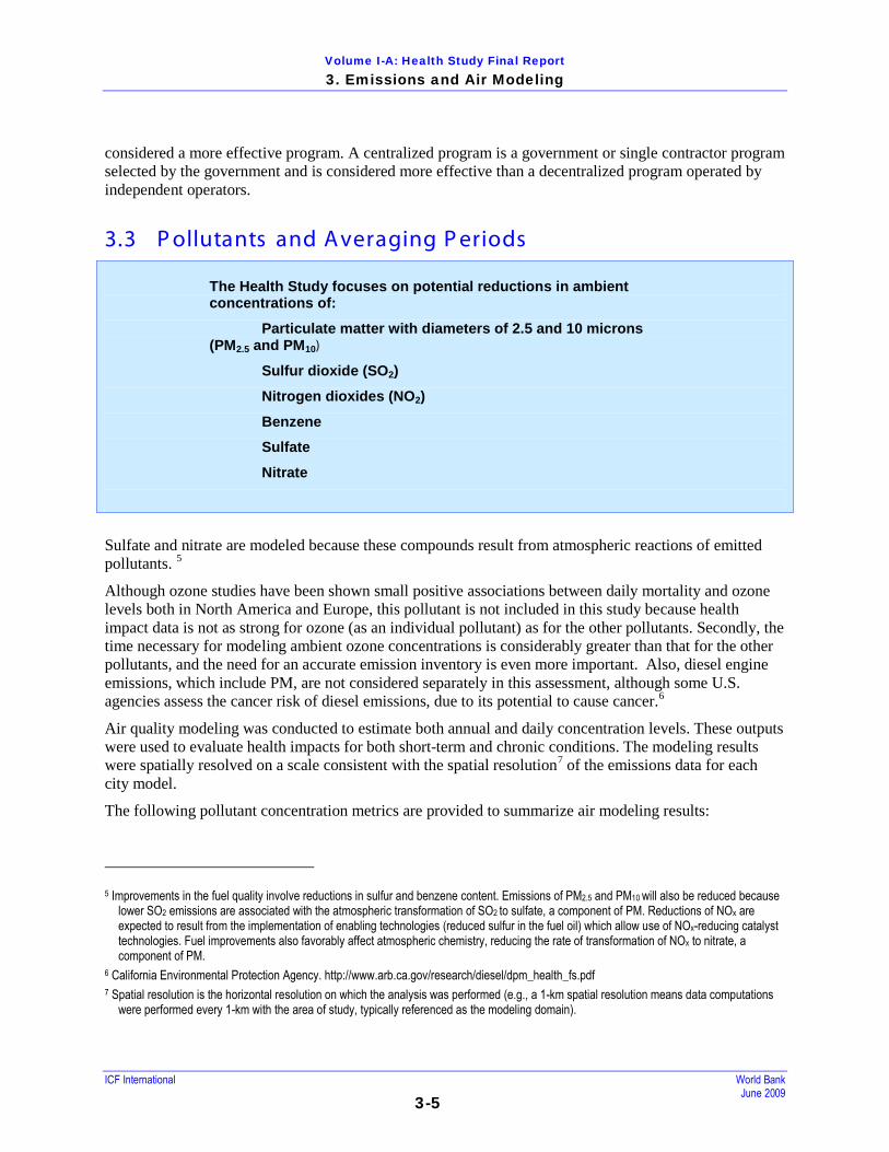
3.3 P ollutants and Averaging P eriods The Health Study focuses on potential reductions in ambient concentrations of:
Particulate matter with diameters of 2.5 and 10 microns (PM2.5 and PM10)
Sulfur dioxide (SO2)
Nitrogen dioxides (NO2)
Benzene
Sulfate
Nitrate
Sulfate and nitrate are modeled because these compounds result from atmospheric reactions of emitted pollutants. 5
Although ozone studies have been shown small positive associations between daily mortality and ozone levels both in North America and Europe, this pollutant is not included in this study because health impact data is not as strong for ozone (as an individual pollutant) as for the other pollutants. Secondly, the time necessary for modeling ambient ozone concentrations is considerably greater than that for the other pollutants, and the need for an accurate emission inventory is even more important. Also, diesel engine emissions, which include PM, are not considered separately in this assessment, although some U.S. agencies assess the cancer risk of diesel emissions, due to its potential to cause cancer.
6
Air quality modeling was conducted to estimate both annual and daily concentration levels. These outputs were used to evaluate health impacts for both short-term and chronic conditions. The modeling results were spatially resolved on a scale consistent with the spatial resolution
7
5 Improvements in the fuel quality involve reductions in sulfur and benzene content. Emissions of PM2.5 and PM10 will also be reduced because
lower SO2 emissions are associated with the atmospheric transformation of SO2 to sulfate, a component of PM. Reductions of NOx are expected to result from the implementation of enabling technologies (reduced sulfur in the fuel oil) which allow use of NOx-reducing catalyst technologies. Fuel improvements also favorably affect atmospheric chemistry, reducing the rate of transformation of NOx to nitrate, a component of PM.
6 California Environmental Protection Agency. http://www.arb.ca.gov/research/diesel/dpm_health_fs.pdf 7 Spatial resolution is the horizontal resolution on which the analysis was performed (e.g., a 1-km spatial resolution means data computations
were performed every 1-km with the area of study, typically referenced as the modeling domain).
of the emissions data for each city model.
The following pollutant concentration metrics are provided to summarize air modeling results:

Volume I-A: Health Study Final Report 3. Emissions and Air Modeling
ICF International World Bank June 2009
3-6
• Minimum Annual Average. An annual average concentration was calculated for each grid points in the modeling domain. The minimum value for each pollutant among all grid points is presented here.
• Annual Average (spatially averaged). The average annual concentration, averaged across the entire modeling domain, is the spatial annual average.
• Maximum Daily Average (spatially averaged). The maximum average daily concentration, averaged across the entire modeling domain, is the spatial daily maximum.
• Maximum Annual Average. An annual average concentration was calculated for each grid point in the modeled area. The maximum value for each pollutant among all grid points is presented.
Concentrations of PM are presented both as primary and total. Primary PM is emitted directly into the atmosphere, and resulting concentrations result from dispersion, whereas secondary PM is formed in the atmosphere through chemical and physical transformation. Total PM is the sum of primary and secondary PM.
3.4 Air Quality Model
3.4.1 Development of E mis s ion Inventories
Emission sources were divided into three groups:
• Vehicle sources
• Industrial sources
• Area sources
Vehicle sources consist of cars and trucks, off-road vehicles, locomotives, watercraft, etc. Data needs for air modeling focus on fleet characteristics and distribution, road characteristics and distribution, fuel mix, and fleet activity and activity distribution. For many cities in Africa, vehicle sources emit the majority of benzene and other volatile organic compounds (VOCs), nitrogen oxides (NOx), particulate matter (PM), and carbon monoxide (CO).
Large industrial sources, such as cement plants, refineries, steel, power plants, and other manufacturing centers, were investigated. Air modeling data needs for industrial sources are focused on facility locations, emission stack parameters, industrial profile and production levels, control technologies, and fuel mix.
Area sources consist of small industrial activities (e.g., wood burning activities, small combustion boilers, refueling stations) and other disperse sources of pollution, such as residential cooking. Area source data needed for air modeling include population distribution, which was used as a surrogate for estimating spatial distribution of diffuse emissions.
In some cases, industrial and vehicle source emissions data (as well as meteorology data, discussed in a subsequent section) come from different years, and this additional uncertainty is noted where appropriate. Technical details of the emissions inventory development are discussed in Appendix C.

Volume I-A: Health Study Final Report 3. Emissions and Air Modeling
ICF International World Bank June 2009
3-7
The Base Case inventory captures present-day estimates of direct emissions of pollutants from vehicle, industry, and area sources. To generate the Base Case inventory, data were collected from published literature, African public officials, researchers in Africa, public and private databases, and internet sources. Vehicle sources include on-road vehicle sources such as passenger vehicles, taxis, light and heavy duty trucks, and motorcycles, and non-road sources such as marine vessels. Re-entrained road dust8 emitted as a result of vehicle traffic on roadways was also considered. Industrial sources were limited to large units (over 250 tons9
For consistency, data for multiple sources (i.e. vehicle and industrial sources) were taken from the same reference where possible. Where preliminary modeling or professional judgment indicated that reference data were unreliable, they were adjusted. Published monitoring data were used as a basis for comparison to determine the reliability of emissions strength. Where local monitoring data were not available, countrywide ambient PM10 concentration estimates were used for comparison purposes, as reported by UNEP.
per year of any one pollutant) emitted at discrete points (i.e. stacks). Area sources are smaller stationary sources that have numerous points of emissions and include household energy production, cooking fires, and fuel stations.
A literature review was conducted to identify pre-existing inventories and literature sources that could provide data for the emissions inventory for each quantitatively assessed city. The literature review used pollutant, location, and source keywords, and surveyed scientific journals and conference proceedings. In addition, internet searches were performed.
10
3.4.1.1 Vehic le S ource Inventory Development
The reliability of each data source was evaluated on a case-by-case basis, with World Bank and UN documents generally being considered most reliable, peer-reviewed journal articles and reports the next most reliable, and uncorroborated internet sources generally least reliable. However, regardless of the reliability of the source, where no other data were available, less reliable sources were incorporated into the inventory. Because no central emissions database was available for the SSA, different methodology for developing the inventory for each modeling location may have been used, depending on the type and reliability of available data. The following subsections describe the process for developing the inventory for each source category.
Additional technical details of the emissions inventory development are presented in Appendix C.
Vehicle sources represent a near source exposure category; therefore, accurately capturing these sources is crucial to predicting the health effects from a change in fuel specifications. For each of the selected cities, when sufficient motor vehicle and traffic characterization information (fleet mix, age and class distribution, vehicle technology distribution, fuel type and vehicle activity such as number of starts and driving patterns) was available, a city-specific emission inventory was developed.
Where an existing vehicle source emission inventory was not available, or where data gaps existed, we used the International Vehicle Emissions Model (IVEM)11
8 Road dust which is re-suspended in the atmosphere by tires moving over paved or unpaved roadways. 9 Unless otherwise noted, all units are metric.
to develop an inventory. IVEM is a motor vehicle computer model designed to estimate emissions from motor vehicles in developing countries. The model is flexibly designed to incorporate region-specific information, which was incorporated when
10 United Nations Environmental Programme. Global Environmental Outlook, GEO Data Portal, Environmental Database. Search results of “Air Quality.” Last Updated: June 2006. Last Accessed: November 25, 2008. http://geodata.grid.unep.ch/
11 International Sustainable Systems Research Center. International Vehicle Emissions Model website. Last Accessed: December 21, 2008. www.issrc.org/ive.

Volume I-A: Health Study Final Report 3. Emissions and Air Modeling
ICF International World Bank June 2009
3-8
available. When region-specific information was unavailable, we used default emission rate values in combination with best available region-specific adjustment factors. The model is adaptable and contains over 700 vehicle technologies, so it can capture a wide range of local fleet characteristics. The region-specific information includes important factors such as gasoline and diesel fuel quality information. The model reports emission factors for SO2, VOC, and NOx, benzene, as well as PM.
The IVEM is capable of estimating emissions for an entire city, and incorporates effects such as lack of vehicle maintenance and gross polluters (e.g., two-stroke motorcycles or heavy diesel engines). The model has been used and tested in a number of developing cities worldwide, including Nairobi, Kenya.12
Additional vehicle sources potentially considered include marine sources (for port cities). Where port activity data was available, these emission sources were included in the vehicle source inventory and calculated according to U.S. Environmental Protection Agency best practices.
Where information was lacking for a selected city, we used the Nairobi data with local adjustments as appropriate. For example, the Nairobi fleet reported an average vehicle age of 11 years. This is generally consistent with many other African studies which report a relatively old fleet.
Output from IVEM (reported as grams of pollutant per kilometer traveled) was combined with transportation activity data (vehicle-kilometers traveled [VKT]) to estimate motor vehicle-related emissions for each selected city. Re-suspended dust from travel on paved and unpaved roads was calculated using vehicle activity information. Details on the calculation of road dust are presented in Appendix C. The emissions from the re-suspended road dust are included in the vehicle emission inventory and relative contribution to PM levels are discussed qualitatively for each target city, so that the health assessment can consider road dust separately from the other sources of PM.
Because traffic-related activity is, as a first approximation, related to population density, vehicle source emissions were allocated in each city based on population density. Population density estimates are based on the LandScan™ dataset, which is discussed in greater detail in Appendix C. Assumed vehicle activity patterns are presented in Appendix C.
13
3.4.1.2 Indus trial S ource Inventory Development
Industrial activities use fuel oil for power generation resulting in air pollutant emissions. Previous investigations of SSA cities have shown that the principal air pollutants from industrial sources are SO2 and, to a lesser degree, PM.14
12 Nairobi, Kenya Vehicle Activity Study, University of California at Riverside and Global Sustainable Systems Research, March 2002.
To identify major contributors to SO2, PM10 and PM2.5 emissions, the following industries were researched: coal-fired power plants, refineries, chemical plants, cement plants,
13 US EPA. Current Methodologies and Best Practices in Preparing Port Emission Inventories, Final Report. US EPA Sector Strategies Program. Prepared by ICF Consulting. January 5, 2006. http://www.epa.gov/ispd/ports/#bestpractices. Only hoteling and maneuvering emissions were included in the inventory. Where transit and cruising emissions occur outside of the inner emissions grid, they were excluded from the analysis.
14 For instance, see the following references: - South African Government Department of Environmental Affairs and Tourism, Draft Report on Emissions Inventories, KZN Province.
http://www.environment.gov.za/HotIssues/2007/Air_quality/docs/Jay%20Puckree%20-%2012h20to12h40.ppt. - Osuji and Avwiri, 2005. Flared Gases and Other Pollutants Associated with Air Quality. - Clean Air Initiative, Banque Mondiale. Burkina Faso. Etude de la qualité de l’air à Ouagadougou. Rapport Final, November 2007. - Clean Air Initiative, Banque Mondiale. Benin. Ministère de l’environnement de de la protection de la nature (MEPN). Etude de la qualité
de l’air à Cotonou. Rapport Final, November 2007.
Volume I-A: Health Study Final Report 3. Emissions and Air Modeling
ICF International World Bank June 2009
3-9
and steel production. We used a cutoff threshold of 250 tons per year as the definition of a major industrial source.15
3.4.1.3 Area S ource Inventory Development
Where local information was available on emission rates and stack parameters, these data were used directly in the analysis. However, in most cases only more general information, such as data on fuel consumption or total emission levels, was available. In these cases, we used information on fuel quality for each country, and equipment and technology specifications, and then estimated emissions of PM and SO2 using the United States Environmental Protection Agency (US EPA) AP-42 emission factors. These emissions factors vary depending on the type of pollution control technology, if any, used. We assumed, in general, that there no pollution control technologies are in use in industries for modeled cities unless evidence to the contrary was available.
Locations of the industrial activity are based on the best available information, such as the location of industrial zones and/or maps with major industrial source locations. In some cases, industrial sources mentioned in a literature source could not be definitively located, and thus were assumed to be sited at facilities identified in satellite photography. Descriptions of city-specific industrial emissions are provided in the regional analysis and in Appendix C.
Air pollution from household wood burning is a significant source of PM10, PM2.5, and NOx in much of SSA. In addition, some emissions of benzene can also be attributed to domestic fuel burning, as discussed further in Appendix C. Emissions estimates from this key source category are based on the best available information available for each modeled city.16
3.4.2 G eophys ic al Data (L and-Us e and T errain E levation)
Spatial allocation of these emissions use the same population distributions as previously discussed for vehicle sources. Other area sources include small combustion boilers and refueling stations. Also, for the South African city modeled, we included emissions from household coal burning.
Detailed methodology for the development of area source inventories are provided for each modeled city in the regional analyses and in Appendix C.
Total domestic fuel burning emissions were allocated to the 1-km2 air quality modeling domain grid cells based on estimated population, as was performed for vehicle sources. The assumed daily pattern of domestic fuel burning emissions, presented in detail in Appendix C, reflects high activity levels associated with morning and evening food preparation, with lower activity for mid-day food preparation.
Land use and terrain information is incorporated into the air quality model through the meteorological model CALMET, described in detail in Appendix C. ICF used published and publicly available land cover data derived from satellite imagery at a 1-km resolution. Digital elevation model (DEM) terrain data for Sub-Saharan Africa was acquired for the region at 90-meter horizontal resolution, and was processed as described in Appendix C.
15 USEPA uses 250 tons per year as the definition of a major emission source. Smaller sources will presumably be included in the area source
emission category. 16 If the city selected for modeling does not have a specific residential wood combustion inventory then we use the methodology as employed in
the World Bank Cotonou study to estimate these emissions. This requires an estimate of wood burning usage by households and the number of household using wood burning for cooking.

Volume I-A: Health Study Final Report 3. Emissions and Air Modeling
ICF International World Bank June 2009
3-10
3.4.3 Meteorologic al Data and Modeling
The CALMET meteorological model (Version 6.326) was used in the analysis. The model uses available hourly surface and twice daily upper air meteorological observational data to enable the air quality model CALPUFF to simulate local meteorological conditions. CALMET makes use of temperature, wind speed and direction, cloud cover, and pressure to develop gridded fields of wind, temperature, surface friction velocity, convective scale velocity, mixing height, Monin-Obkhov length, and atmospheric stability classes. The upper air and representative hourly surface data details and methodology for each quantitatively studied city are presented in Appendix C.
3.4.4 C AL P UF F Modeling
The latest version of the CALPUFF air quality model was used in this study (Version 6.4)17
Total PM was calculated by adding primary PM (from direct emissions) with sulfate (SO4) and nitrate (NO3) on an hourly basis. Daily and yearly averages were computed with these adjusted total PM values. Nitrogen dioxide (NO2) concentrations were also calculated on an hourly basis using ozone limiting, effectively limiting each hourly average concentration to a maximum of 78.4 µg/m3 plus the 10 percent NOx emitted as NO2; this assumes a regional background ozone concentration of 40 ppb (78.4 µg/m3).
. The CALPUFF modeling system uses hourly meteorological data from CALMET in combination with hourly emission rate information to simulate the transport, dispersion and, for some species, the chemical transformation, of air pollutants. One year of modeling was performed and ambient concentrations were obtained for each hour at each model grid cell for each modeled city. Results were aggregated to daily average and yearly average concentrations in each of the grid cells. Subsequently, results were aggregated separately for grid cells with greater than 1,000 people per kilometer, to focus the air results on those areas of the cities with the greatest density of people.
18
3.5 R egional Analys es
The CALPUFF modeling options used in this analysis are based on physical processes that are important in determining the changes in air concentrations as a result of fuel quality improvements. The modeling options are chosen so that all of the important physical processes that may be encountered in the transformation and distribution of air pollutants are included in the modeling. The key CALPUFF modeling options used are described in Appendix C.
The following sections provide inventory development and model specifications, as well as a summary of results.
3.5.1 E as tern R egion
3.5.1.1 Quantitative Analys is – K ampala, Uganda
The emerging megacity of Kampala is located to the north of Lake Victoria, the largest inland freshwater lake on Earth. The city serves as both the economic and political capital of Uganda. Kampala sits atop a
17 US EPA. 2008. CALPUFF Modeling System. http://www.epa.gov/scram001/dispersion_prefrec.htm#calpuff. 18 Vingarzan, R. 2004. Atmospheric Environment, A review of surface ozone background levels and trends, Atm Env., 38, 21: 3421-3442.
Volume I-A: Health Study Final Report 3. Emissions and Air Modeling
ICF International World Bank June 2009
3-11
plateau and terrain features many rolling hills and wetlands in the outlying areas. Key environmental problems identified by Matagi (2002) include: poor solid waste collection, inadequate sewer and sanitation facilities, insufficient drainage (probably related to development of wetlands), motor vehicle traffic pollution, industrial pollution, and runoff from urban agriculture. In addition, the challenges of urban poverty within Kampala complicate efforts toward sustainable development.19
3.5.1.1.1 E mis s ion Inventories
Matagi (2002) provides a useful overview of environmental issues facing Kampala, and this document was used as primary background for the emissions inventory development.20
Vehicle Source Emissions
Matagi provides descriptions of industrial activities along with an industrial map that formed the basis for many of the industrial source assumptions. Appendix C provides detailed, technical information about the development of the inventory for Kampala.
For Kampala, motor vehicle and general traffic characterization information was available from which to develop a city-specific emission inventory. However, no vehicle source emission factors were available, thus the International Vehicle Emissions Model (IVEM) (www.issrc.org/ive) was used to develop the vehicle source emission factors.
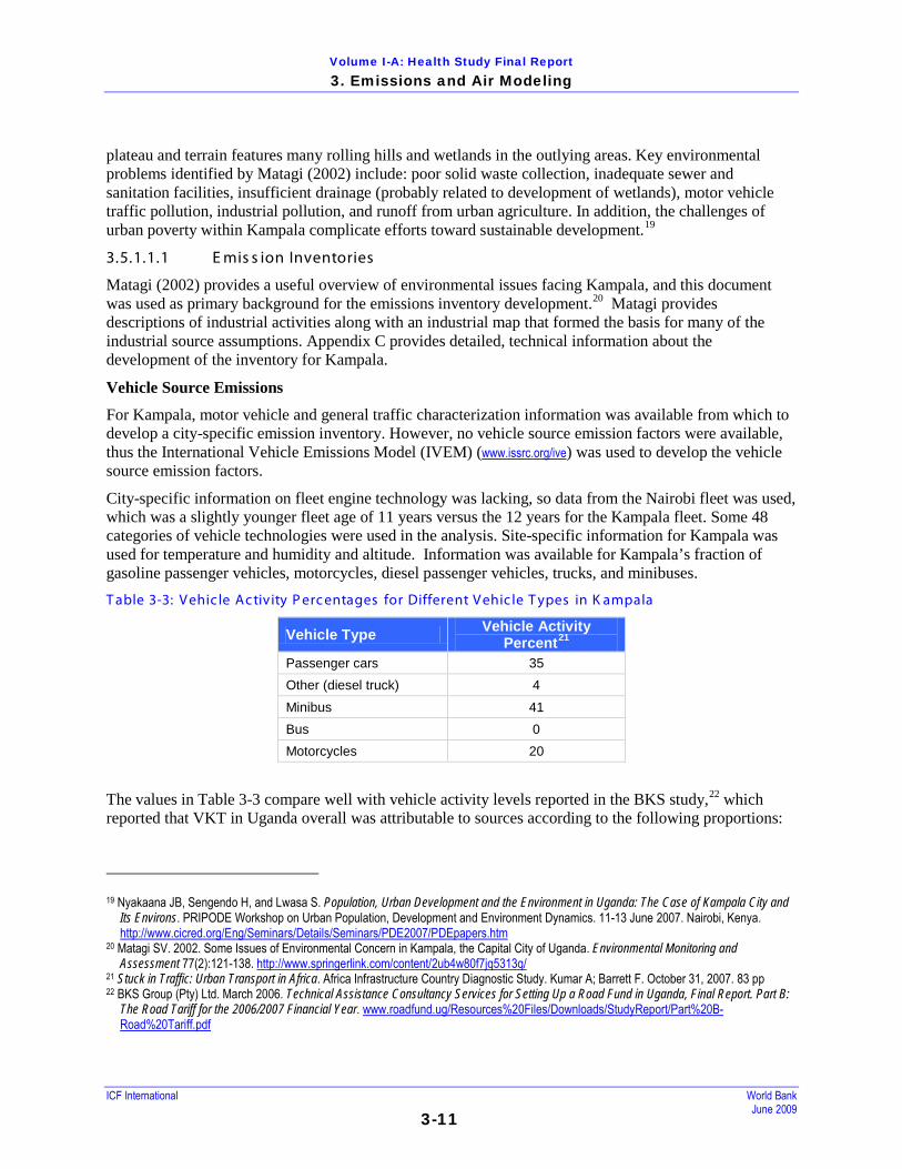
City-specific information on fleet engine technology was lacking, so data from the Nairobi fleet was used, which was a slightly younger fleet age of 11 years versus the 12 years for the Kampala fleet. Some 48 categories of vehicle technologies were used in the analysis. Site-specific information for Kampala was used for temperature and humidity and altitude. Information was available for Kampala’s fraction of gasoline passenger vehicles, motorcycles, diesel passenger vehicles, trucks, and minibuses. T able 3-3: Vehic le Ac tivity P erc entages for Different Vehic le T ypes in K ampala
Vehicle Type Vehicle Activity Percent21
Passenger cars 35 Other (diesel truck) 4
Minibus 41 Bus 0 Motorcycles 20
The values in Table 3-3 compare well with vehicle activity levels reported in the BKS study,22
19 Nyakaana JB, Sengendo H, and Lwasa S. Population, Urban Development and the Environment in Uganda: The Case of Kampala City and
Its Environs. PRIPODE Workshop on Urban Population, Development and Environment Dynamics. 11-13 June 2007. Nairobi, Kenya.
which reported that VKT in Uganda overall was attributable to sources according to the following proportions:
http://www.cicred.org/Eng/Seminars/Details/Seminars/PDE2007/PDEpapers.htm 20 Matagi SV. 2002. Some Issues of Environmental Concern in Kampala, the Capital City of Uganda. Environmental Monitoring and
Assessment 77(2):121-138. http://www.springerlink.com/content/2ub4w80f7jq5313q/ 21 Stuck in Traffic: Urban Transport in Africa. Africa Infrastructure Country Diagnostic Study. Kumar A; Barrett F. October 31, 2007. 83 pp 22 BKS Group (Pty) Ltd. March 2006. Technical Assistance Consultancy Services for Setting Up a Road Fund in Uganda, Final Report. Part B:
The Road Tariff for the 2006/2007 Financial Year. www.roadfund.ug/Resources%20Files/Downloads/StudyReport/Part%20B-Road%20Tariff.pdf

Volume I-A: Health Study Final Report 3. Emissions and Air Modeling
ICF International World Bank June 2009
3-12
• 43 percent private vehicles
• 16 percent commercial vehicles
• 21 percent public transport vehicles
• 21 percent motorcycles
However, since these values are for all of Uganda, and are not specific to Kampala, the numbers presented in Table 3-3 were selected over the values for all of Uganda.
Other information required for the model was from the Nairobi fleet, as described in Appendix C.
Baseline fuel characteristics assumed premixed gasoline with a sulfur content of 600 ppm and 3 percent benzene content by volume and average sulfur content in diesel fuel of 5,000 ppm. These specifications were based on figures provided by the Steering Committee. Though benzene content in fuel may be as high as 5 percent, the maximum average concentration available in IVEM is 3 percent. City-specific fleet average emission output for each pollutant from IVEM (grams of pollutant per kilometer traveled) was then combined with VKT to estimate vehicle-related emissions for Kampala.
Emissions for re-entrained road dust for Kampala were estimated based on the fraction of paved and unpaved roads and the vehicle kilometers traveled on those fractions along with local silt loading.
Total vehicle activity within Kampala has been reported as 798 million VKT, of which 750 million (94 percent) occurs on paved surfaces.23
Alternate 2-Stroke Motorcycle VKT Assumptions
Since no measure or distribution of VKT was available for Kampala, population distribution was used as a surrogate for allocating vehicle source emissions throughout a city grid mapped to population distribution. Because actual vehicle emissions are dictated by VKT on roadways and not by population distribution, this assumption may result in some spatial misallocation of vehicle source emissions. For instance, though population in commercial districts may be low relative to residential areas, vehicle activity (particularly truck activity) is probably higher in these areas compared to population weighted activity levels.
No marine vessel inventory was assembled for Kampala, though it has an active port on Lake Victoria. No vessel call list was obtained by the study team, and it was assumed that while marine vessel impacts may have impact on local air quality, city-wide effects would be small compared to impacts from other emission sources. In any case, the recent actions of the International Maritime Organization (IMO) to revise the wording of Annex VI of the MARPOL agreement will result in a global effort, starting in 2012, to reduce the sulfur content of marine fuels. The target level for the sulfur content of marine fuels by 2020 is 0.5% which will substantially reduce the SO2 levels around ports.
Emissions from motorcycles are a function of the total activity of motorcycles. The motorcycle travel fraction for Kampala was based on published vehicle activity data for that city, as described above.
However, the Steering Committee expressed concern that the Health Study emissions inventory under-represented motorcycle emissions in Kampala, Uganda (for which results are then extrapolated to the east SSA region) for the Base Case and Scenario 1.24
23 BKS Group (Pty) Ltd. March 2006. Technical Assistance Consultancy Services for Setting Up a Road Fund in Uganda, Final Report. Part B:
The Road Tariff for the 2006/2007 Financial Year.
These concerns were based on limited observations that
www.roadfund.ug/Resources%20Files/Downloads/StudyReport/Part%20B-Road%20Tariff.pdf
24 Scenario 2 assumes a complete phase-out of 2-stroke motorcycles.

Volume I-A: Health Study Final Report 3. Emissions and Air Modeling
ICF International World Bank June 2009
3-13
motorcycle use has increased in recent years in East Africa. Some data regarding motorcycle purchases and use are available to support these observations, but while counts of vehicle types are useful when vehicle activity data are not available, emissions are not directly scalable with vehicle counts. For instance, though buses make up a small fraction of vehicles in most cities, they are frequently operated on a nearly continual basis, meaning that emissions from buses are not proportional to their number. Therefore, whenever possible, the preferred choice is the travel fraction data as a basis for vehicle activity, which is a nearly proportional to emissions. However, quantitative data on the vehicle activity levels of 2-stroke motorcycles were not identified for Kampala. Nevertheless, based on the Steering Committee direction, the air modeling results were adjusted using the following assumption:
• East SSA Region: VKT from 2-stroke motorcycles was increased from 20% to 50% for the Base Case and Scenario 1
Note that only the air modeling results are scaled (alternate results shown in Table 3-11). The emissions results discussed below (Tables 3-5 through 3-6) and the initial air modeling results (Tables 3-7 through 3-10) are based on the initially described emissions assumptions.
Scenario 1 - Implementation of AFRI-4 Fuel
For Scenario 1, average values of 50 ppm sulfur and 0.5 percent benzene for gasoline and 50 ppm for sulfur in diesel were assumed. These sulfur values differ from the AFRI-4 specifications (150 ppm S and 1.0 percent benzene in gasoline) because IVEM only allows a discrete set of sulfur fractions. These represent the closest values below the fuel specifications. This difference in sulfur fractions between the actual fuel specifications and the available values for sulfur in IVEM is not expected to have a major impact on PM emissions because the PM contribution from gasoline fueled vehicles is small in comparison to diesel fueled vehicles which emit PM at about 10 to 100 times higher rate than gasoline vehicles when PM control technologies are not employed. No adjustments were made for increased vehicle kilometers traveled, increased number of vehicles, changes in vehicle technology, or fleet fuel fraction in Scenario 1. IVEM was re-run with these fuel-specific changes and resulting emissions were calculated assuming the vehicle activity levels remained the same. Substantial motor vehicle tailpipe emissions reductions over the Base Case were seen for SO2 (1,747 metric tons per year [tpy] to 8 tpy, a reduction of 99.5 percent), total PM (556 to 460 tpy, a reduction of 17 percent), and benzene (610 to 279 tpy, a reduction of 54 percent) (Tables 3-4 and 3-5).
Scenario 2 - AFRI-4 Fuel, 80% of Vehicles with Emissions Control Technology, and 20% Increase in VKT
In Scenario 2 IVEM was set to average values of 50 ppm sulfur and 0.5 percent benzene for gasoline and 50 ppm for sulfur in diesel. This maximum level of sulfur content will need to be reached to enable the use of advanced emissions control systems (advanced catalysts systems and particulate filter systems which are being used to meet EURO IV and US EPA Tier 2 standards) that are capable of significantly reducing air pollutants.
The modeled vehicle source tailpipe emissions in Scenario 2 (Table 3-6) are reduced by about 11 percent for NOx, 57 percent for total PM, and 96 percent for benzene over changes in fuel specifications only (Scenario 1) (Table 3-5). However, SO2 emissions increase by 20 percent with the additional VKT growth, as current emission control technology does not reduce SO2 emissions.
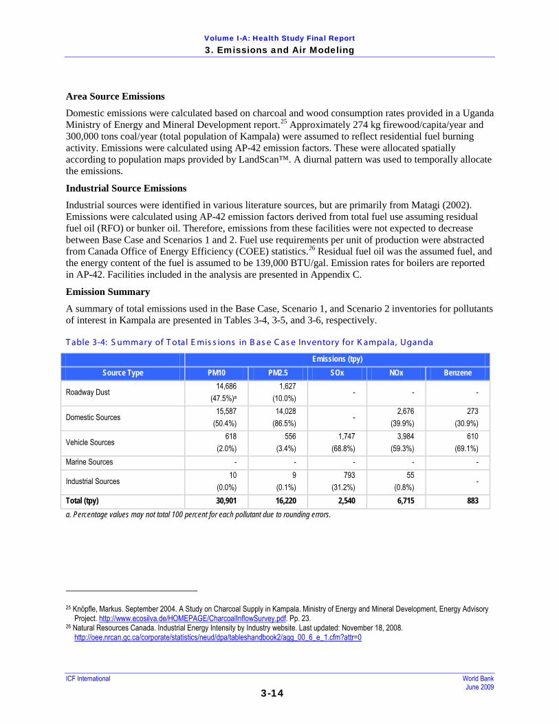
Volume I-A: Health Study Final Report 3. Emissions and Air Modeling
ICF International World Bank June 2009
3-14
Area Source Emissions
Domestic emissions were calculated based on charcoal and wood consumption rates provided in a Uganda Ministry of Energy and Mineral Development report.25
Industrial Source Emissions
Approximately 274 kg firewood/capita/year and 300,000 tons coal/year (total population of Kampala) were assumed to reflect residential fuel burning activity. Emissions were calculated using AP-42 emission factors. These were allocated spatially according to population maps provided by LandScan™. A diurnal pattern was used to temporally allocate the emissions.
Industrial sources were identified in various literature sources, but are primarily from Matagi (2002). Emissions were calculated using AP-42 emission factors derived from total fuel use assuming residual fuel oil (RFO) or bunker oil. Therefore, emissions from these facilities were not expected to decrease between Base Case and Scenarios 1 and 2. Fuel use requirements per unit of production were abstracted from Canada Office of Energy Efficiency (COEE) statistics.26
Emission Summary
Residual fuel oil was the assumed fuel, and the energy content of the fuel is assumed to be 139,000 BTU/gal. Emission rates for boilers are reported in AP-42. Facilities included in the analysis are presented in Appendix C.
A summary of total emissions used in the Base Case, Scenario 1, and Scenario 2 inventories for pollutants of interest in Kampala are presented in Tables 3-4, 3-5, and 3-6, respectively.
T able 3-4: S ummary of T otal E mis s ions in B as e C as e Inventory for K ampala, Uganda
Emissions (tpy) Source Type PM10 PM2.5 SOx NOx Benzene
Roadway Dust 14,686
(47.5%)a 1,627
(10.0%) - - -
Domestic Sources 15,587
(50.4%) 14,028
(86.5%) -
2,676 (39.9%)
273 (30.9%)
Vehicle Sources 618
(2.0%) 556
(3.4%) 1,747
(68.8%) 3,984
(59.3%) 610
(69.1%) Marine Sources - - - - -
Industrial Sources 10
(0.0%) 9
(0.1%) 793
(31.2%) 55
(0.8%) -
Total (tpy) 30,901 16,220 2,540 6,715 883 a. Percentage values may not total 100 percent for each pollutant due to rounding errors.
25 Knöpfle, Markus. September 2004. A Study on Charcoal Supply in Kampala. Ministry of Energy and Mineral Development, Energy Advisory
Project. http://www.ecosilva.de/HOMEPAGE/CharcoalInflowSurvey.pdf. Pp. 23. 26 Natural Resources Canada. Industrial Energy Intensity by Industry website. Last updated: November 18, 2008.
http://oee.nrcan.gc.ca/corporate/statistics/neud/dpa/tableshandbook2/agg_00_6_e_1.cfm?attr=0

Volume I-A: Health Study Final Report 3. Emissions and Air Modeling
ICF International World Bank June 2009
3-15
T able 3-5: S ummary of T otal E mis s ions in S cenario 1 Inventory for K ampala, Uganda
Emissions (tpy) Source Type PM10 PM2.5 SOx NOx Benzene
Roadway Dust 14,686
(47.7%)a 1,627
(10.1%) - - -
Domestic Sources 15,587
(50.6%) 14,028
(87.0%) -
2,676 (40.1%)
273 (49.4%)
Vehicle Sources 511
(1.7%) 460
(2.9%) 8
(1.0%) 3,950
(59.1%) 279
(50.5%) Marine Sources - - - - -
Industrial Sources 10
(0.0%) 9
(0.1%) 793
(99.0%) 55
(0.8%) -
Total (tpy) 30,794 16,124 801 6,681 553 a. Percentage values may not total 100 percent for each pollutant due to rounding errors.
T able 3-6: S ummary of T otal E mis s ions in S cenario 2 Inventory for K ampala, Uganda
Emissions (tpy) Source Type PM10 PM2.5 SOx NOx Benzene
Roadway Dust 14,686
(48.1%)a 1,627
(10.3%) - - -
Domestic Sources 15,587
(51.1%) 14,028
(88.4%) -
2,676 (42.8%)
273 (96.4%)
Vehicle Sources 220
(0.7%) 198
(1.2%) 10
(1.2%) 3,524
(56.3%) 10
(3.4%) Marine Sources - - - - -
Industrial Sources 10
(0.0%) 9
(0.1%) 793
(98.8%) 55
(0.9%) -
Total (tpy) 30,503 15,862 803 6,255 283 a. Percentage values may not total 100 percent for each pollutant due to rounding errors.
3.5.1.1.2 R eceptors – Air Quality Monitors
No air monitoring data was available for Kampala. This is a serious deficiency in air quality research for Kampala that has been identified by others (e.g., Schwela). Data from the UNEP was used for model comparison in this case. Annual average concentrations of PM10 in east SSA, which likely underestimate the concentration in Kampala, reportedly average 48µg/m3, with a range between 16 and 88 µg/m3.27
27 United Nations Environmental Programme. Global Environmental Outlook, GEO Data Portal, Environmental Database. Search results of “Air
Quality.” Last Updated: June 2006. Last Accessed: November 25, 2008.
http://geodata.grid.unep.ch/

Volume I-A: Health Study Final Report 3. Emissions and Air Modeling
ICF International World Bank June 2009
3-16
3.5.1.1.3 K ampala Air Modeling R es ults and Dis cus s ion
Base Case modeling results for Kampala are presented in Table 3-7. Scenario 1 and Scenario 2 results are presented in Tables 3-8 and 3-9.
T able 3-7: B as e C as e Modeling R es ults for K ampala, Uganda
Metric (µg/m3) Primary PM2.5
Primary PM10
Total PM2.5
Total PM10 SO2 SO4 NO2 NO3 HNO3 Ben-
zene Minimum Annual Average 9 16 9 16 0.8 0.0 1.8 0.1 0.5 0.4 Annual Average (spatially averaged) 127 212 127 213 9.8 0.3 20.0 0.6 3.2 5.6
Maximum Daily Average (spatially averaged) 350 631 358 637 34.1 3.2 35.2 8.1 25.5 18.0
Maximum Annual Average 703 1,155 705 1,157 50.4 0.7 68.9 1.2 8.7 30.0
T able 3-8: S cenario 1 (AF R I-4 F uel S pec ific ations ) Modeling R es ults for K ampala, Uganda
Metric (µg/m3) Primary PM2.5
Primary PM10
Total PM2.5
Total PM10 SO2 SO4 NO2 NO3 HNO3 Ben-
zene Minimum Annual Average 9 16 9 16 0.0 0.0 1.8 0.1 0.5 0.3 Annual Average (spatially averaged) 126 211 126 212 0.5 0.0 20.0 0.6 3.2 3.5
Maximum Daily Average (spatially averaged) 348 629 355 632 1.5 0.1 35.1 8.1 25.4 11.2
Maximum Annual Average 699 1,151 700 1,152 4.9 0.0 68.8 1.2 8.7 18.8
T able 3-9: S cenario 2 (AF R I-4 F uel S pec ific ations with C ontrol T ec hnologies ) Modeling R es ults for K ampala, Uganda
Metric (µg/m3) Primary PM2.5
Primary PM10
Total PM2.5
Total PM10 SO2 SO4 NO2 NO3 HNO3 Ben-
zene Minimum Annual Average 9 16 9 16 0.0 0.0 1.7 0.1 0.4 0.1 Annual Average (spatially averaged) 124 209 124 210 0.5 0.0 19.2 0.6 3.0 1.8
Maximum Daily Average (spatially averaged) 342 623 348 626 1.5 0.1 34.0 7.5 23.7 5.7
Maximum Annual Average 688 1,140 689 1,141 4.9 0.0 67.9 1.1 8.2 9.6
These results show that the reduction in gasoline benzene content with the AFRI-4 fuel specifications has a pronounced effect with the spatially averaged annual average benzene concentration reduced from a baseline of 5.6 µg/m3 to 3.5 for Scenario 1 and to 1.8 µg/m3 for Scenario 2 over the whole of the Kampala domain. For Scenario 1, reduction in diesel and gasoline sulfur content reduces spatial annual average SO2 concentrations from 9.8 to 0.5 µg/m3
through fuel changes only. PM is only marginally affected since emissions are dominated by roadway dust and domestic sources in the Kampala model (see Tables 3-3, 3-4, and 3-5). NO2 concentrations for Scenario 2 are reduced in proportion to the small change in emissions

Volume I-A: Health Study Final Report 3. Emissions and Air Modeling
ICF International World Bank June 2009
3-17
of this compound seen over the Base Case. The annual average PM10 concentrations are higher than those reported by UNEP (16 to 88 µg/m3; average of 48 µg/m3), however, the UNEP results are for the whole eastern Africa region and thus may not be comparable to the city of Kampala.
The results presented above include areas of high and low population density. It is of greater interest for the purposes of this study to determine the concentrations to which most individuals are exposed. Therefore, Table 3-10 presents the modeled annual average (spatially averaged) concentrations for Kampala in densely populated areas (>1,000 people per sq. km). The vast majority of the population (93.6 percent) in the modeling domain falls within the densely populated areas, so the results more closely reflect actual ambient exposure concentrations in populated areas of Kampala. Because only 34.6 percent of cells were selected for the density analysis, the results may be expected to differ somewhat from the full domain results. Indeed, concentrations are between 16.7 and 76.6 percent higher in the densely populated areas than averaged over the full domain.
T able 3-10: Modeled Annual Average (S patially Averaged) Air C ontaminant C onc entrations in Dens ely P opulated Areas - K ampala
Scenario PM2.5 PM10 Total PM2.5
Total PM10 SO2 SO4 NO2 NO3 HNO3 Ben-
zene Base 223 370 224 371 16.7 0.4 33.2 0.8 4.5 9.7 Scenario 1 221 368 222 369 0..7 0.0 33.1 0.8 4.5 6.1 Scenario 2 218 365 219 366 0.7 0.0 31.9 0.7 4.2 3.1
As discussed in Section 3.5.1.1.1, the air modeling results were scaled to incorporate alternate assumptions for Kampala, that is higher 2-stroke motorcycle use in the west SSA region than had been assumed. The scaled air modeling results are shown below, and are used in this report’s health and benefit assessments. T able 3-11: Alternate As s umptions : Modeled Annual Average (S patially Averaged) Air C ontaminant C oncentrations in Dens ely P opulated Areas - K ampala
Scenario PM2.5 PM10 Base 226.77 373.50 Scenario 1 224.61 371.41 Scenario 2 218.50 365.52
3.5.1.2 Qualitative Analys is – Nairobi, K enya
A template for the qualitative analysis process is presented in Appendix A.
Nairobi lies approximately five hundred kilometers to the east-south-east of Kampala, and is the capital and largest city of Kenya with a population of 2,948,109.28 The terrain is gently rolling, with rocky hills to the west and south-west, and large mountains far to the north and southeast (Mounts Kenya and Kilimanjaro). Nairobi is 1,661 m above sea level, approximately 500 m higher in elevation than Kampala, and has a relatively moderate climate, with moderate rainfall that peaks in the early fall.29
28 City Population website – Kenya. www.CityPopulation.de/Kenya.html. 29 Nairobi climate information. http://www.wordtravels.com/Cities/Kenya/Nairobi/Climate
The average

Volume I-A: Health Study Final Report 3. Emissions and Air Modeling
ICF International World Bank June 2009
3-18
population density in Nairobi is 4,310 people per square kilometer, as the city covers an area of approximately 684 sq km.30 Nairobi is therefore approximately thirty percent more populous than and twice as densely populated as Kampala. The city functions as a major industrial center of Kenya with most of the manufacturing work related to processing of agricultural products. However, emissions in Nairobi originate predominantly from an aging fleet of poorly maintained vehicles and open air burning of household wastes, wood, and charcoal. Emissions from industries are of less importance.31
T able 3-12: Air P ollution E mis s ion S ummary for Nairobi, K enya
Air monitoring in Kenya is performed on an ad hoc basis (that is, there is no national program). Table 3-12 contains an emission inventory for Nairobi.
VOCs (metric tons/year [t/y]) NOx (t/y) SO2 (t/y) PM10 (t/y) PM2.5 (t/y)
Industrial Sources a 19,933 6,639 2,911 1,030 927 Domestic Sources - 5,762 b,c,e - 62,625 b,c,e 56,363 f
Vehicle Sources 199,325 66,392 29,114 10,300 9,270 Road Dust - - - 246,123 31.496 Marine Sources N/A N/A N/A N/A N/A Total 219,258 b-d 78,793 b-d 32,025 b-d 350,078 98,056 a. Schwela 2006.31 b. World Health Organization (WHO). Country Profiles of Environmental Burden of Disease-Kenya. Geneva. 2007. Public Health and the Environment. http://www.who.int/quantifying_ehimpacts/national/countryprofile/kenya.pdf c. Nzioka, 2008.32
d. Dutch National Institute for Public Health (RIVM) and Netherlands Organization for Applied Scientific Research (TNO). 2001. The Emission Database for Global Atmospheric Research (EDGAR) 3.2. Precursors: NMVOC (Non-Methane Volatile Organic Compounds): Aggregated Emissions 1990/1995. The Netherlands: RIVM.
http://arch.rivm.nl/env/int/coredata/edgar/. e. World Bank Development Data Center. Energy Production and Use. Table 3.7. 2005 World Development Indicators. http://devdata.worldbank.org/wdi2005/Section3.htm f. Calculated using 90 percent factor based on PM10 emissions. In order to calculate the emissions from domestic sources for NOx, SO2, and PM10, first the consumption of combustible renewables and waste in Nairobi was estimated by multiplying this consumption in Kenya (2005 World Development Indicators) by the ratio of the populations in Nairobi and Kenya as was done for total emissions. This consumption value in Nairobi was multiplied by the chemical-specific emission factor to get the chemical-specific consumption values for domestic sources in Nairobi. The emission factors for all pollutants were assumed to be the same as those used for Kampala. The estimated emissions from domestic sources for PM2.5 were estimated by multiplying the emissions value for PM10 by 90 percent, which is a standard assumption for combustion source emissions of PM2.5 as a fraction of PM10.
Calculation of vehicle source emissions was based on assumed total vehicle activity levels and a vehicle fleet similar to that of Kampala. This calculation is described below. Industrial emissions were uniformly assumed to be 10 percent of vehicle emissions, based on a statement that industrial emissions were of less 30 City of Nairobi Environmental Outlook. Executive Summary. 2007 City Council of Nairobi.
http://www.unep.org/DEWA/Africa/docs/en/NCEO_Report_FF_New_Text.pdf 31 Schwela D. 2006. Review of Urban Air Quality in Sub-Saharan Africa Region - Air Quality profile of SSA countries, provided by World Bank
6/12/08. 32 Solomon M. Nzioka. June 30, 2008. Needs Assessment for Centralized Road Traffic Accidents Surveillance Unit As Basis For Evidence-
Based Public Healthy Policy Management On Road Traffic Accidents In Nairobi, Kenya. Epidemiological Basis for Decision Making in Health Administration. http://www.scribd.com/doc/3708784/Vision-2030-Rethinking-Road-Traffic-Accidents-RTAs-Management-in-Nairobi-Kenya.

Volume I-A: Health Study Final Report 3. Emissions and Air Modeling
ICF International World Bank June 2009
3-19
importance than vehicle emissions, and this fraction is somewhat consistent with industrial activity levels assumed for Kampala.33
Sixty percent of all vehicles in Kenya (850,000)
34 were assumed to be in Nairobi (510,000), as was done
for Kampala. This value for total number of vehicles in Nairobi was multiplied by the percentages of different modes of transport to get vehicle counts by different modes of transportation (e.g., bus, matatu). These vehicle counts by mode of transportation were multiplied by the VKT per vehicles from Cape Town to get the VKT per mode of transportation. The calculated percentage of VKT from motorcycles is very small: only 2 percent. This finding and the calculated VKT distribution are consistent with distributions reported by Davis et al. (2005).35
3.5.1.3 Qualitative Analys is – Dar E s S alaam, Tanzania
The total calculated vehicle activity in Nairobi was estimated at 13,300 million VKT, which is more than 16 times the vehicle activity reported for Kampala. No published data was available to validate this calculation. Vehicle emissions were calculated by multiplying vehicle emissions from Kampala by this ratio; therefore, identical diesel and petrol fuel fractions were assumed for the two cities: 45 percent diesel and 55 percent petrol. Total PM10 and PM2.5 levels in road dust were estimated through the same process as for Kampala using these same VKT values and fraction of travel on paved roads.
If the emissions estimates presented in Table 3-12 are approximately accurate, emissions from vehicle travel may have a large impact on health, especially due to particulate matter. However, much of the projected impact is from road dust, which is most readily controllable through paving roads. Due to large uncertainties in the inventory for Nairobi, the magnitude of motor vehicle contribution to ambient PM levels could not be confirmed. Even so, PM2.5 emissions from vehicles represent only 9 percent of all such emissions, with the majority due to domestic sources of open air burning of household wastes, wood, and charcoal, and due to road dust. Still, improvement in fuel quality and vehicle quality and technology will have a comparatively larger impact in Nairobi than that in Kampala because of the large amount of traffic. We anticipate that the changes in fuel in Scenario 1 and Scenario 2 would have the most important effect on reducing benzene concentrations in the air in Nairobi, possibly reducing annual average benzene concentrations by up to a factor of 3. Ambient concentrations of SO2 should show much larger reductions with the introduction of clean fuels than Kampala owing to the much larger fraction of SO2 emissions attributable to motor vehicles.
Like Kampala, the population and economic activity of Nairobi are expected to increase markedly over the coming decades, though there is a high level of uncertainty about the level of economic growth, especially considering the current global economic downturn. As motor vehicles have been identified as a primary cause of poor air quality in Nairobi, improvement in fuel quality and vehicle technology may significantly alleviate air quality problems especially when considered over the large urban population and over large time intervals.
Dar Es Salaam is a large, port city on the Indian Ocean coast in East Africa, approximately 1,000 km to the southeast of Kampala. The city functions as the primary administrative, social, and economic hub of Tanzania, with a population of approximately 2.5 million people.36
33 Schwela 2006. 34 Proceedings of the Regional Workshop on Better Air Quality in the Cities of Africa. Indaba Hotel, Johannesburg, S. Africa. April 21 – 23,
2004. Part 4. 35 Davis N, Lents J, Osses M, Nikkila N, and Barth M. 2005. Development and Application of an International Vehicle Emissions Model. TRB
Paper No. 05-1844. https://www.u-cursos.cl/ingenieria/2007/2/ME65A/1/material_docente/objeto/151771
Table 3-13 contains an emission
36 2002 Tanzania Census Tables. http://www.tanzania.go.tz/census/tables.htm.

Volume I-A: Health Study Final Report 3. Emissions and Air Modeling
ICF International World Bank June 2009
3-20
inventory for Dar Es Salaam estimated from the global EDGAR 32FT2000 emission inventory.37 Estimated emission data for NOx, and SOx is provided on a 1 degree by 1 degree grid. The emission data was multiplied by the ratio of city area to total grid area to yield values for the city of Dar Es Salaam. Industrial emissions for Dar Es Salaam were obtained from the UNEP’s Urban Air Quality Management Toolbook.38
T able 3-13: E s timated E mis s ions for Dar E s S alaam C ity, T anzania for Indus try and Other S ources
In 1993, before the company installed pollution control equipment, the Wazo Hill Cement Factory accounted for approximately 95 percent of all industrial particulate emissions, at 106,000 tpy (of total 111,293 tpy). Because reported TSP emissions at Wazo Hill are disproportionately higher than NOx or SO2 emissions, we assume that this inventory includes all facility operations. It was further assumed that all TSP emissions were in the form of PM10. Installation of particulate control equipment is assumed to mitigate emissions by 50 percent, to 55,647 tpy. Emissions from marine sources could not be estimated, because a call list from the Port was not available.
PM10 (t/y) PM2.5 (t/y) NOx (t/y) SOx (t/y) Benzene (t/y) Industrial 55,647 50,082 1,215 453 - Domestic Sources 19,366 17,429 - 3,325 339
Vehicle Sources 442 398 1,250 2,851 436 Road Dust 10,717 1,176 - - -
Marine Sources Unavailable Unavailable 1,287 Unavailable Unavailable Total 86,173 69,086 3,752 6,629 776
The city of Dar Es Salaam accounts for almost half of the total vehicles in Tanzania, accommodating more than an 110,000 vehicles.39 Approximately 55 percent of the total vehicles operate on diesel fuel, while the remaining 45 percent are powered by petrol. Per Wilson and Gashaza,40
The road network of Dar Es Salaam consists of approximately 1,140 km of paved roads, of which 445 km, or 39 percent, are paved (Wilson and Gashaza, 2004). Per Jackson (2005),
the percentage of cars was assumed to be 46.81 percent, buses 7.94 percent, goods trucks 29.17 percent, motorcycles 10.80 percent, tractors/earth movers 2.71 percent, and trailers 2.57 percent.
41
37 Olivier, J.G.J., Van Aardenne, J.A., Dentener, F., Ganzeveld, L. and J.A.H.W. Peters (2005). Recent trends in global greenhouse gas
emissions: regional trends and spatial distribution of key sources. In: "Non-CO2 Greenhouse Gases (NCGG-4)", A. van Amstel (coord.), page 325-330. Millpress, Rotterdam, ISBN 90 5966 043 9. Available at
the total vehicle activity on major city routes was calculated to be approximately 571 million VKT. Road dust is calculated using the same methodology as was used for Kampala, and assuming that VKT fractions are proportional to
http://www.aero.jussieu.fr/projet/ACCENT/EDGAR32_metadata.php. The city of Dar es Salaam lies between longitude 39° and 39° 33’ east and between latitudes 6° 33’ and 7° 1’. Because the grid between longitude 39° and 40° and between latitudes 6° and 7 reported estimated emissions of zero, the grid between longitude 38° and 39° and between latitudes 6° and 7° was used.
38 United Nations Environmental Program (UNEP) (2006). Urban Air Quality Management Toolbook. http://ww2.unhabitat.org/wuf/2006/aqm/index.htm. Emissions of PM are reported as TSP (total suspended particulates), which we assume to be completely from boilers, thus 100 percent PM10.
39 Feresu, S., S. Simukanga, G. Haq, K. Hicks, and D. Schwela (2004). Proceedings of the Regional Workshop on Better Air Quality in the Cities of Africa. Indaba Hotel, Johannesburg, S. Africa. April 21–23, 2004. Available at http://www.sei.se/baq.html.
40 Wilson, L. and J. R. Gashaza (2004). Proceedings of the 23rd Southern African Transport Conference (SATC). Pretoria, S. Africa. July 12–15, 2004. Available at https://www.up.ac.za/dspace/bitstream/2263/5677/1/Wilson_Transport(2004).pdf.
41 Jackson, M. M. (2005). Roadside concentrations of gaseous and particulate matter pollutants and risk assessment in Dar es Salaam, Tanzania. Environmental Monitoring and Assessment 104: 385–407.

Volume I-A: Health Study Final Report 3. Emissions and Air Modeling
ICF International World Bank June 2009
3-21
vehicle fractions. IVEM was not used to calculated vehicle emissions. Instead, a similar vehicle mix to that of Kampala is assumed for Dar Es Salaam for the purposes of calculating vehicle emissions. Emissions are scaled by VKT. Emissions from domestic sources were estimating by scaling from Kampala by population.
Given that diesel vehicles make up a large portion of the vehicle fleet (45 percent, identical to the fleet mix of Kampala), and that the assumed base fuel quality is low (5,000 ppm S in diesel, 600 ppm S in petrol), we expect to find similar results to Kampala in Dar Es Salaam from reducing sulfur in fuel. Similar to Kampala, we anticipate that the change in fuel specifications would have the most important effect on reducing benzene concentrations and would reduce annual average benzene concentrations by up to a factor of 3. Ambient concentrations of SO2 should show somewhat larger reductions in Dar es Salaam compared to Kampala with the introduction of clean fuels, owing to the larger fraction of SO2 emissions attributable to motor vehicles. However, we anticipate that in the vicinity of the Port there would be little change in ambient SO2 concentration levels owing to the high sulfur content residual fuel use by marine vessels. The Port has a capacity to 3.1 million tons of general cargo, 1 million tons of containers, and 6 million tons of liquid bulk.42
42 Tanzania Port Authority. Dar es Salaam port.
Emissions from the Port were estimated by subtracting all other emission sources from total emission levels. This differential was assumed to be completely attributable to the Port. The recent actions of the International Maritime Organization (IMO) to revise the wording of Annex VI of the MARPOL agreement will result in a global effort, starting in 2012, to reduce the sulfur content of marine fuels. The target level for the sulfur content of marine fuels by 2020 is 0.5 percent, which will substantially reduce the SO2 levels around ports. Similar to Kampala, no change is expected in ambient PM2.5 concentrations owing to the large fraction of PM2.5 concentrations from re-entrained road dust and domestic sources of open air burning of household wastes, wood, and charcoal. Note that somewhat lower ambient PM concentration levels are anticipated for Dar Es Salaam compared to Kampala because of its coastal location with generally higher annual average wind speeds (i.e., better ventilation).
Table 3-14 provides a summary of the qualitative analyses of Nairobi, Kenya, and Dar Es Salaam, Tanzania, by comparison to the quantitative analysis for Kampala, Uganda.
http://www.tanzaniaports.com/dsm/index.htm. Website accessed February 13, 2009.

Volume I-A: Health Study Final Report 3. Emissions and Air Modeling
ICF International World Bank June 2009
3-22
T able 3-14: Qualitative As s es s ment for the E as tern S S A R egion (B as ed on C omparis on with K ampala)
Key Factors Comparison to Reference City (Kampala,
Uganda) Resulting Impact
Effect on
Conc. References and Notes
Nairobi Vehicle contribution to PM emissions
Vehicle PM emissions contribute approximately 3 percent of total PM10 and 9.5 percent of PM2.5 emissions in Nairobi, compared to 2 and 3.4 percent, respectively, for Kampala.
Vehicles tailpipe emissions of PM may be 50 percent more responsible for PM10 emissions and nearly 200 percent more responsible for PM2.5 emissions in Nairobi as compared to Kampala.
See Tables 3-4 and 3-10 for methods, values, and notes
Diesel vehicle share
Assumed ratio of gasoline to diesel fueled vehicles similar to Kampala.
Changes in fuel for Scenario 1 and Scenario 2 scenarios would have the most important effect on reducing benzene concentrations; estimated impact similar to Kampala reducing annual average benzene concentrations by up to a factor of 3.
Kumar and Barrett 2007
Base fuel quality Assume same fuel quality as in Kampala for Nairobi.
No impact.
Marginal improvement in fuel quality under Scenario 1
Both Nairobi and Kampala will use fuel consistent with AFRI-4 standards under Scenario 1.
Because VKT may be higher in Nairobi, marginal improvement may be greater there.
See Footnote 45
Emission control in existing vehicle fleet
Assume same emission controls as in Kampala for Nairobi.
No impact.
Area source fuel and distribution
Similar emission distribution and practices in regards to domestic fuel burning from wood and charcoal.
PM2.5 concentrations estimated to be similar.
See text
Industrial emissions
Industrial emissions in Nairobi were assumed to be considerably larger (650 times, for PM2.5) than for Kampala.
Targeting industrial sector emissions through improved fuel and technology may be more effective in Nairobi than in Kampala.
Schwela 2006
Other Factors Dar Es Salaam Vehicle contribution to PM emissions
The diesel vehicle share is higher in Dar Es Salaam than in Kampala
Vehicle tailpipe emissions of PM may have a stronger impact on ambient concentrations than in Kampala
Wilson and Gashaza 2004
Diesel vehicle share
Higher fraction of diesel vehicles as share of total fleet compared to Kampala.
Vehicle tailpipe emissions of PM may have a stronger impact on ambient concentrations than in Kampala
Wilson and Gashaza 2004
Base fuel quality Assume same fuel quality as in Kampala.
No impact.

Volume I-A: Health Study Final Report 3. Emissions and Air Modeling
ICF International World Bank June 2009
3-23
T able 3-14: Qualitative As s es s ment for the E as tern S S A R egion (B as ed on C omparis on with K ampala)
Key Factors Comparison to Reference City (Kampala,
Uganda) Resulting Impact
Effect on
Conc. References and Notes
Marginal improvement in fuel quality under Scenario 1
Diesel fuel quality improves considerably between Base Case and Scenario 1
Improved fuel quality will have greater impact in Dar es Salaam than Kampala
Emission control in existing vehicle fleet
Assume same emission controls as in Kampala.
No impact.
Area source fuel and distribution
Similar emission distribution and practices in regard to domestic fuel burning and road dust emissions, but with coastal location leading to improved ventilation on average.
PM concentrations estimated to be lower.
See text
Industrial emissions
Ratio of industrial SO2 to motor vehicle emissions in Kampala is larger than for Dar Es Salaam.
Reduced sulfur in fuels will show greater impact on reducing ambient SO2 concentrations.
See emission inventories Tables 3-4 and 3-11
Other Factors No port in Kampala. Dar Es Salaam has an active port.
Port activities in Dar Es Salaam estimated independently based on higher industry wide residual fuel oil average sulfur content of 2.6% (with a cap of 4.5%); ambient levels of SO2 and PM likely higher in port vicinity.
3.5.1.4 Qualitative Analys is – S ummary of R es ults for E as t S S A R egion
The qualitative assessment used the results from the quantitative assessment of Kampala, Uganda, to predict the potential effects of fuel quality improvements in two other cities:
• Nairobi – Vehicles may account for 91% of SOx emissions in Nairobi, compared to 69% in
Kampala – Vehicle contribution to PM2.5 emissions in Nairobi (14%) may be much higher than for
Kampala (3.4%) – Reduced sulfur in fuel will have a larger impact in Nairobi
• Dar Es Salaam – Contribution of SO2 from road sources in Dar Es Salaam (43%) is somewhat lower than
that of Kampala (69%) – Contribution of PM2.5 from road vehicles in Dar Es Salaam (0.6%) is much lower than
that of Kampala (3.4%) – Better PM control on vehicles will have much smaller effect in Dar Es Salaam compared
to Kampala
Volume I-A: Health Study Final Report 3. Emissions and Air Modeling
ICF International World Bank June 2009
3-24
3.5.2 Wes tern R egion
3.5.2.1 Quantitative Analys is – C otonou, B enin
Cotonou is the economic capital of Benin, as well as its largest city, housing two-thirds of Benin's industries. Its urban area continues to expand, notably towards the west. The city is a major port, located on the coastal strip between Lake Nokoué and the Atlantic Ocean. The city is cut in two by a canal, the lagoon of Cotonou. The Oueme River flows into the Atlantic Ocean at Cotonou.
Data for vehicle use for Cotonou show that a large percentage of VKT is associated with 2-stroke motorcycles. Thus, as discussed in Section 6, regionalizing the Cotonou analysis is problematic because some large cities in West Africa, particularly some states of Nigeria, have banned 2-stroke engines. While 2-stroke engines have not entirely disappeared from those cities, their prevalence has decreased to the point that using Cotonou’s inventory for other east SSA cities may not be realistic. Thus, the results for the west SSA region have been scaled downward, as described in this section.
3.5.2.1.1 E mis s ions Inventory
A full emissions inventory was developed for Cotonou in 2007 under the World Bank Clean Air Initiative program43
Vehicle Source Emissions
(hereafter called the World Bank Cotonou study). This inventory was the primary source of data for the Cotonou emissions inventory, adjusted as noted below. Additional technical information about the development of the emission inventory is presented in Appendix C.
The World Bank Cotonou inventory contains a well-developed vehicle source inventory (vehicle type, engine size, and fuel type), which uses fuel consumption as the basis for estimating the 2005 vehicle source inventory. However, this inventory was developed assuming a maximum permitted level of sulfur in diesel of 10,000 ppm and a gasoline sulfur content of 1,500 ppm with 6.8% benzene. This, in combination with the need to develop a more consistent set of underlying assumptions to facilitate intercomparison between the three SSA cities modeled, steered us to model the vehicle source emissions using the same emission factor model, the IVEM model, as was used in the other two cities. The model used the data collected in the World Bank Cotonou study, which included the fleet vehicle mix and fleet activity data.
According to the World Bank Cotonou study, in 2005 Cotonou had 28,221 diesel engine and 112,885 gasoline engine passenger vehicles, as well as about 18,000 light and heavy duty diesel trucks. The majority of vehicles in Cotonou are 2- and 4-stroke motorcycles, with approximately 266,000 on the road. The vehicle types were combined with vehicle activity data (VKT) to estimate total vehicle activity levels in Cotonou that were used in the analysis, as described in detail in Appendix C (Table 3-15).
43 Clean Air Initiative, Banque Mondiale. Benin. Ministère de l’environnement de la protection de la nature (MEPN). Etude de la qualité de l’air à
Cotonou. Rapport Final, November 2007. (Translation from French to English.) (World Bank Cotonou study)

Volume I-A: Health Study Final Report 3. Emissions and Air Modeling
ICF International World Bank June 2009
3-25
T able 3-15: V ehic le Ac tivity P ercentages for Different Vehic le T ypes in C otonou
Vehicle Type Vehicle Activity
Percent44
Passenger cars 31.1
Light trucks (<3.5 t) 11
Mid-size trucks (>3.5 t to <7.5 t)
0
Heavy trucks (> 7,5 t) 0
4-stroke motorcycles 9.5
2-stroke motorcycles 48.4
Emissions of NOx, SOx, PM10, and VOCs, as well as road dust emissions (PM), are provided in the World Bank Cotonou study. The World Bank Cotonou study assumed that 90 percent of the total VKT takes place on paved roads and the remaining 10 percent on unpaved roads in Benin. This is likely an over-prediction of travel on unpaved roads; therefore, we applied a 95/5 split for paved/unpaved VKT, lowering PM10 emissions from re-entrained road dust by 49 percent.
Emissions of PM2.5 were calculated from PM10, assuming that 90 percent of combustion sources are PM10 and 10 percent of road dust is PM2.5. However, based on preliminary modeling results, road dust emissions as estimated in the World Bank Cotonou study appeared to be overestimated. The World Bank study relied on road dust emission factors that appear to be 5.3 times higher than those recommended by the US EPA AP-42 methodology for roadway re-entrainment. Even the AP-42 factors are considered to be very conservative (overestimating road dust emissions), thus, the re-entrained road dust from unpaved roads could be considerably lower, by as much as half, depending upon local soil characteristics and the generally high humidity environments (WRAP 2006). Therefore, road dust emissions reported in the World Bank Cotonou study were reduced by a factor of 2.
The city-specific emission inventory was spatially allocated for SO2, NOx, VOC, PM10 and PM2.5, accounting for emissions from passenger vehicles, light and heavy trucks, and 2- and 4-stroke motorcycles. Since no measure of distribution of VKT was available, population distribution was used as a surrogate for allocating vehicle source emissions. Because actual motor vehicle emissions are dictated by VKT on roadways and not by population distribution, this assumption may result in some spatial misallocation of vehicle source emissions. For instance, though population in commercial districts may be low respective to residential areas, vehicle activity (particularly truck activity) is probably higher in these areas compared to population weighted activity levels. Also, different types of vehicles may be more prominent in some parts of the city than in others. For instance, poorer areas of the city may have higher rates of 2-stroke engine motorcycle use compared to the average rates.
The World Bank Cotonou study assumed that 80 percent of urban emissions in Benin are from Cotonou. This assumption is similar to the qualitative analysis performed for Ouagadougou, Burkina Faso, for
44 Derived from data presented in the World Bank Cotonou study (see Appendix C).

Volume I-A: Health Study Final Report 3. Emissions and Air Modeling
ICF International World Bank June 2009
3-26
which the assumption was from the Burkina Faso Ministry of Transport.45
Since Cotonou is an important port city with high port volume, marine vessel emissions could be a source of air pollutants. No changes were assumed for marine vessels although the recent actions of the International Maritime Organization (IMO) to revise the wording of Annex VI of the MARPOL agreement will result in a global effort, starting in 2012, to reduce the sulfur content of marine fuels. The target level for the sulfur content of marine fuels by 2020 is 0.5% which will substantially reduce the SO2 levels around ports. Marine traffic levels were obtained from the Cotonou Port authority.
Although this assumption appeared to overestimate emissions for the city, 80 percent was used for inventory development.
Fuel characteristics were based on a best estimate of actual fuel characteristics as follows:
Sulfur in Gasoline – 600 ppm S
Sulfur in Diesel – 5,000 ppm S
Benzene (gasoline only) – 3 percent
Emissions for re-entrained road dust are estimated based on the fraction of paved and unpaved roads and the VKT on those fractions, in combination with estimates of on-road local silt loading.
46
Alternate 2-Stroke Motorcycle VKT Assumptions
A marine vessel emissions inventory using these traffic data was developed using the U.S. Environmental Protection Agency (EPA) methodology and allocated as area sources limited to three cells in the south of the air quality modeling domain. Bunker fuel sulfur content was assumed to be between 2.7 and 4.5 percent, depending on the ship engine type. Emissions were assumed to be spread evenly across all hours and all days of the year.
Emissions from motorcycles are a function of the total activity of motorcycles. We based the assumptions for motorcycle travel fraction in Cotonou on published vehicle activity data, as described above.
The Steering Committee expressed concern that the Health Study emissions inventory over-represented motorcycle emissions in Cotonou (for which results are then extrapolated to the west SSA region) in the Base Case and Scenario 1.47 These concerns were based on observations that 2-stroke motorcycle use has decreased in recent years in West Africa because some large cities, particularly in Nigeria, have banned 2-stroke engines. While 2-stroke engines have not entirely disappeared from those cities, their prevalence has decreased to the point that using Cotonou’s inventory for Nigerian cities may not be realistic. Shares of modes of transport are presented in Table 3-16, which is reproduced from a 2007 report provided to ICF by the World Bank.48
45 Clean Air Initiative, Banque Mondiale. Burkina Faso. Etude de la qualité de l’aiir à Ouagadougou. Rapport Final, November 2007.
(Translation from French to English.) Hereafter, the World Bank Ouagadougou inventory.
As shown, there are some cities in West Africa that have similar motorcycle prevalence as Cotonou - Ouagadougou and Bamako are examples. Other cities have very few motorcycles, such as Douala, Dakar, and Lagos.
46 Port Autonome de Cotonou, DACC/SESP. Evolution du trafic des navires: Periode de 1996 a 2005. http://www.portdecotonou.com/trafics.php. (Translation from French to English.)
47 Scenario 2 assumed the complete phase-out of 2-stroke motorcycles. 48 Stuck in Traffic: Urban Transport in Africa. Africa Infrastructure Country Diagnostic Study. Kumar A; Barrett F. October 31, 2007.

Volume I-A: Health Study Final Report 3. Emissions and Air Modeling
ICF International World Bank June 2009
3-27
T able 3-16. S hares of Modes of T rans port in Us e in 14 Afric an C ities
C ity R egion
(new c olumn) L arge
bus Minibus T axi Motorc yc le P rivate
c ar Walk Other
Abidjan W 11 19 29 0 18 22 1
Accra W 10 52 9 0 13 12 4
Addis Ababa E 35 20 5 0 7 30 3
Bamako W 1 10 5 56 19 — 9
Conakry W 1 14 6 0 1 78 0
Dakar W 3 73 6 6 11 — 1
Dar es Salaam E 1 15 6 2 29 39 8
Douala W 10 — 13 12 2 60 3
Kampala E 0 41 — 20 35 — 4
Kigali E 1 75 10 0 10 5 0
Kinshasa W — — — — — High —
Lagos W 10 72 6 6 5 High 1
Nairobi E 7 29 15 2 — 47 0
Ouagadougou W 8 0 — 58 14 — 20
Average 7 30 8 12 12 37 4 (Reproduced from: Stuck inTraffic: Urban Transport in Africa. Africa Infrastructure Country Diagnostic Study, p.5.)
Some general data regarding motorcycle purchases and use are available to support these observations, but while counts of vehicle types are useful when vehicle activity data are not available, emissions are not directly scalable with vehicle counts. Therefore, whenever possible, we used travel fraction data as a basis for vehicle activity, which is nearly proportional to the emissions. However, since quantitative data on the vehicle activity levels of 2-stroke motorcycles were not identified for Cotonou, in order to extrapolate the Cotonou analysis to the west SSA region, the air modeling results were scaled using the following assumptions:
• West SSA Region: VKT from 2-stroke motorcycles was reduced from 50% to 10% for the Base Case and Scenario 1
Note that only the air modeling results are scaled (alternate air modeling results shown in Table 3-24). The emissions results discussed below (Tables 3-17 through 3-19) and the initial air modeling results (Tables 3-20 through 3-23) are based on the published vehicle activity data.
Scenario 1 - Implementation of AFRI-4 Fuel
For Scenario 1, sulfur content in diesel fuel was reduced, as specified in the input to IVEM, from the assumed baseline value of 5,000 ppm to 50 ppm, while gasoline sulfur was reduced from the assumed baseline value of 600 ppm to 50 ppm. These sulfur values differ from the AFRI-4 specifications (150 ppm S and 1.0 percent benzene in gasoline) because IVEM only allows a discrete set of sulfur fractions, and these represent the closest allowable values below the fuel specifications. This difference in sulfur fractions between the actual fuel specifications and the available values for sulfur in IVEM is not expected to have a significant impact on PM emissions because the PM contribution from gasoline-fueled

Volume I-A: Health Study Final Report 3. Emissions and Air Modeling
ICF International World Bank June 2009
3-28
vehicles is small in comparison to diesel-fueled vehicles which emit PM at a rate about 10 to 100 times higher than gasoline vehicles when PM control technologies are not employed. The IVEM model emission factors were then paired with the VKT to result in the Cotonou emission inventory.
The percentage change in motor vehicle tailpipe PM emissions are less (3.4%) than those seen in Kampala (17.3%), mostly attributable to the larger fraction of diesel vehicles in Kampala (45%) versus 17% in Cotonou. Diesel vehicles PM emission rates are more sensitive to reductions in sulfur fuel content than are gasoline vehicles.
Scenario 2 - AFRI-4 Fuel, 80% of Vehicles with Emissions Control Technology, and 20% Increase in VKT
For Scenario 2, the modeled vehicle source emissions are reduced by some 23 percent for NOx, 82 percent for PM and 98 percent for benzene over Scenario 1. The percentage change reductions from Scenario 1 to Scenario 2 for benzene are similar to Kampala; NOx and PM reductions are smaller for Kampala at 11% and 57%, respectively. This is due to the higher diesel fleet fraction in Kampala for which vehicle diesel control technology is less effective at reducing NOx and PM emissions.
Area Source Emissions
Area sources were abstracted from the World Bank Cotonou study and assume that 80 percent of national domestic fuel burning occurs within Cotonou, which is likely an overestimate. Further, the methodology assumes that the emission factor for domestic wood burning is 50 g per kg of wood burned; this is considerably higher than the USEPA AP-42 which estimates a PM10 factor of only 17.3 g per kg of wood burned from residential fireplaces. However, this factor is variable and is a function of a number of wood characteristics and operating practices.
Industrial Source Emissions
Based on information from the World Bank Cotonou study and other documents, a limited industrial inventory was constructed. Emissions sources included three palm oil plants, a cement plant, a brewery and bottling plant, and a large shrimp processing plant. Total industrial emissions reported in the World Bank Cotonou inventory were allocated to each of these facilities. Since no facility-specific stack or emission rate information was available for these facilities the US EPA National Emission Inventory database of default stack parameters was used; this source contains default stack parameters for over 800 industrial classes. All industrial facilities were assumed to operate 365 days per year and 24 hours per day, at a constant rate. In the Base Case, fuel is assumed to be heavy fuel oil and in Scenarios 1 and 2, diesel fuel (subject to AFRI-4 specifications). All industrial sources were assumed to have no control technology installed, based on a qualitative statement to that effect in the World Bank Cotonou study. Seven industrial facilities were modeled in the city, and were positioned in the industrial area, as specified in the land use map presented in Figure 3-2. This figure was overlaid on Google Earth satellite imagery to match with the model location.
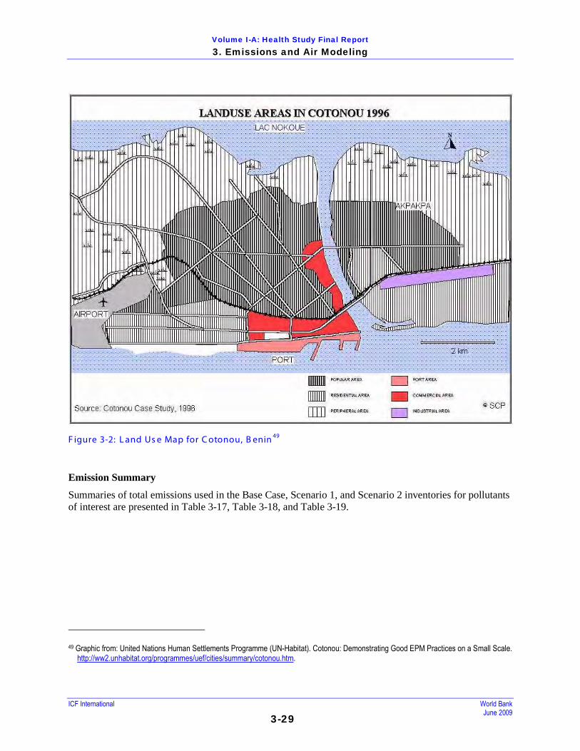
Volume I-A: Health Study Final Report 3. Emissions and Air Modeling
ICF International World Bank June 2009
3-29
F igure 3-2: L and Us e Map for C otonou, B enin 49
Emission Summary
Summaries of total emissions used in the Base Case, Scenario 1, and Scenario 2 inventories for pollutants of interest are presented in Table 3-17, Table 3-18, and Table 3-19.
49 Graphic from: United Nations Human Settlements Programme (UN-Habitat). Cotonou: Demonstrating Good EPM Practices on a Small Scale.
http://ww2.unhabitat.org/programmes/uef/cities/summary/cotonou.htm.

Volume I-A: Health Study Final Report 3. Emissions and Air Modeling
ICF International World Bank June 2009
3-30
T able 3-17: S ummary of T otal E mis s ions in B as e C as e Inventory for C otonou, B enin
Emissions (tpy) Source Type PM10 PM2.5 SOx NOx Benzene
Roadway Dust 6,179
(35.5%)a 618
(5.8%) - - -
Domestic Sources 6,943
(39.9%) 6,249
(58.8%) -
1,377 (6.9%)
127 (2.4%)
Vehicle Sources 3,990
(22.9%) 3,591
(33.8%) 762
(23.7%) 16,497
(83.1%) 5,245
(97.6%)
Marine Sources 169
(1.0%) 156
(1.5%) 1,253
(39.0%) 1,744
(8.8%) -
Industrial Sources 120
(0.7%) -
1,199 (37.3%)
235 (1.2%)
-
Total (tpy) 17,401 10,613 3,215 19,853 5,372 a. Percentage values may not total 100 percent for each pollutant due to rounding errors.
T able 3-18: S ummary of T otal E mis s ions in S c enario 1 Inventory for C otonou, B enin
Emissions (tpy) Source Type PM10 PM2.5 SOx NOx Benzene
Roadway Dust 6,179
(35.8%)a 618
(5.9%) - - -
Domestic Sources 6,943
(40.3%) 6,249
(59.6%) -
1,377 (7.0%)
127 (4.9%)
Vehicle Sources 3,855
(22.4%) 3,470
(33.1%) 45
(2.4%) 16,363
(83.0%) 2,466
(95.1%)
Marine Sources 169
(1.0%) 156
(1.5%) 1,253
(67.3%) 1,744
(8.8%) -
Industrial Sources 90
(0.5%) -
564 (30.3%)
235 (1.2%)
-
Total (tpy) 17,236 10,492 1,862 19,719 2,592 a. Percentage values may not total 100 percent for each pollutant due to rounding errors.

Volume I-A: Health Study Final Report 3. Emissions and Air Modeling
ICF International World Bank June 2009
3-31
T able 3-19: S ummary of T otal E mis s ions in S c enario 2 Inventory for C otonou, B enin
Emissions (tpy) Source Type PM10 PM2.5 SOx NOx Benzene
Roadway Dust 6,179
(43.9%)a 618
(8.1%) - - -
Domestic Sources 6,943
(49.3%) 6,249
(81.7%) -
1,377 (8.6%)
127 (70.2%)
Vehicle Sources 699
(5.0%) 629
(8.2%) 43
(2.3%) 12,642
(79.0%) 54
(29.8%)
Marine Sources 169
(1.2%) 156
(2.0%) 1,253
(67.4%) 1,744
(10.9%) -
Industrial Sources 90
(0.6%) -
564 (30.3%)
235 (1.5%)
-
Total (tpy) 14,080 7,652 1,860 15,998 180 a. Percentage values may not total 100 percent for each pollutant due to rounding errors.
3.5.2.1.2 R eceptors – Air Quality Monitors
Data from two air quality monitors was compared to modeling results for model evaluation and adjustment. Two monitoring locations are discussed in the World Bank Cotonou study. Monitor locations, reproduced from the World Bank Cotonou study, are presented in Figure 3-3. It is not known how representative samples from these monitors may be of the city at large. Areas of uncertainty include:
• The monitors are in the same geographic region and may reflect lower or higher concentrations than those experienced in other parts of the city.
• The monitoring period (2-week intervals) is not directly comparable to model results.
Measurements, each spanning a 24-hour period, of PM10 at the two monitoring locations in southern Cotonou were taken at intervals between March and July, 2007. Observations ranged between a daily minimum of 21 µg/m3 and 454 µg/m3. The study authors regarded an average observation of 78 µg/m3 as representative of annual average concentrations in Cotonou. This is a factor of 6.5 lower than the PM10 concentration predicted by the Base Case modeling, as presented in Table 3-16 below. The over-prediction of PM10 concentrations may be the result of an overestimate of PM10 emissions, particularly from road dust and/or domestic cooking sources.

Volume I-A: Health Study Final Report 3. Emissions and Air Modeling
ICF International World Bank June 2009
3-32
F igure 3-3: C otonou Monitoring L oc ations Figure reproduced from the World Bank Cotonou Inventory.
3.5.2.1.3 C otonou Air Modeling R es ults and Dis cus s ion
Base Case modeling results for Cotonou are presented in Table 3-20. Scenario 1 and Scenario 2 results are presented in Tables 3-21 and 3-22.
T able 3-20: B as e C as e Modeling R es ults for C otonou
Metric (µg/m3) PM2.5 PM10 Total PM2.5
Total PM10 SO2 SO4 NO2 NO3 HNO3 Ben-
zene Minimum Annual Average 20 28 21 29 1.0 0.0 9.4 0.3 1.0 5.7 Annual Average (spatially averaged) 324 505 325 506 21.8 0.2 58.2 0.8 7.2 142.9
Maximum Daily Average (spatially averaged) 845 1,292 851 1,298 52.4 1.1 71.9 10.0 44.3 349.0
Maximum Annual Average 1,026 1,647 1,028 1,648 71.0 0.6 78.0 1.4 14.4 502.4

Volume I-A: Health Study Final Report 3. Emissions and Air Modeling
ICF International World Bank June 2009
3-33
T able 3-21: S c enario 1 Modeling R es ults (AF R I-4 F uel S pec ific ations ) for C otonou
Metric (µg/m3) PM2.5 PM10 Total PM2.5
Total PM10 SO2 SO4 NO2 NO3 HNO3 Ben-
zene Minimum Annual Average 20 28 20 29 0.2 0.0 9.3 0.3 1.0 2.9 Annual Average (spatially averaged) 321 502 322 503 3.0 0.0 58.2 0.8 7.1 69.5
Maximum Daily Average (spatially averaged) 837 1,283 842 1,289 7.5 0.2 71.8 10.0 44.0 170.2
Maximum Annual Average 1,015 1,634 1,016 1,635 25.0 0.1 78.0 1.4 14.3 242.8
T able 3-22: S c enario 2 Modeling R es ults (AF R I-4 F uel S pec ific ations with C ontrol T echnologies ) for C otonou
Metric (µg/m3) PM2.5 PM10 Total PM2.5
Total PM10 SO2 SO4 NO2 NO3 HNO3 Ben-
zene Minimum Annual Average 17 25 18 25 0.2 0.0 8.4 0.2 0.8 0.4 Annual Average (spatially averaged) 246 418 246 419 2.9 0.0 56.6 0.7 5.8 5.7
Maximum Daily Average (spatially averaged) 654 1,080 659 1,085 7.4 0.2 70.9 8.0 35.7 15.1
Maximum Annual Average 753 1,343 754 1,344 25.0 0.1 77.7 1.2 11.8 17.9
For PM10, concentrations are dominated by emissions of road dust (41 percent of PM10 in the Base Case) and domestic emissions (46 percent of PM10 in the Base Case). The vast majority of road dust is from vehicle travel on unpaved roads (assumed to be 5 percent for this city). Vehicle sources subject to AFRI-4 specifications account for only 11 percent of total PM10 emissions in the Base Case. In Scenario 1, the reduction in annual average PM concentrations results entirely from the higher quality fuel specifications. Annual average concentrations of sulfate (SO4) and nitrates (NO3) also show reductions with the use of AFRI-4 fuel specifications and emission control technology reducing concentrations to 0 and 0.8 µg/m3, respectively. For SOx, the relative importance of marine sources nearly doubles, particularly for locations near the port. NOx emissions remain unchanged. Annual average benzene concentrations show the largest percent reduction (51 percent) as a result of switching to AFRI-4 fuel specifications (Scenario 1) and an additional 92 percent reduction with vehicle control technologies (Scenario 2).
Domestic emissions increase in relative importance for PM2.5, especially in Scenario 2, suggesting that in the future, if the assumed improvements in fuel quality and vehicle pollution control equipment are implemented, efforts to reduce outdoor PM should be directed at reducing wood burning as a fuel source.
PM10 from re-entrained road dust is responsible for nearly half of the PM10 emissions. Of this amount more than 97 percent is due to travel on unpaved roads. Significant uncertainty surrounds the use of an appropriate silt loading for unpaved roads - implicit in this inventory is a silt loading of 12 percent; this is higher than the average mid-range value which ranges from 1.8 to 35 percent based on USEPA AP-4250
50 US EPA. Emission Factors and AP-42. Last updated September 2008.
. The silt loading represents the amount of loose dry surface dust which is re-suspended with vehicle
http://www.epa.gov/ttn/chief/ap42/

Volume I-A: Health Study Final Report 3. Emissions and Air Modeling
ICF International World Bank June 2009
3-34
traffic. At the low end re-entrained road dust may be 6.5 times lower than the value used here or potentially 3 times higher. Location-specific roadway tests and/or soil data are needed to reduce this level of uncertainty.
The total PM results are higher than the available monitoring data. This is likely because emissions from road dust and domestic sources are overestimated for Cotonou, in addition to the potential over-allocation of these emissions to Cotonou from the Benin inventory. However, it is the incremental change is important to this study.
The results presented above include areas of high and low population density. It is of greater interest for the purposes of this study to determine the concentrations to which most individuals are exposed. Therefore, Table 3-23 presents the modeled annual average (spatially averaged) concentrations for Cotonou in densely populated areas (>1,000 people per sq. km). Nearly all of the population (99.6 percent) in the modeling domain falls within the densely populated areas, so the results more closely reflect actual ambient exposure concentrations in populated areas of Cotonou. Because 76 percent of cells were selected for the density analysis, the results may be expected to remain mostly consistent with the full domain results. Indeed, concentrations are only between 6.7 and 12.7 percent higher in the densely populated areas than averaged over the full domain.
T able 3-23: Modeled Annual Average (S patially Averaged) Air C ontaminant C onc entrations in Dens ely P opulated Areas - C otonou
Scenario PM2.5 PM10 Total PM2.5
Total PM10 SO2 SO4 NO2 NO3 HNO3 Ben-
zene Base 362 566 363 567 24.4 0.2 62.6 0.9 7.9 161.1 Scenario 1 359 562 359 563 3.2 0.0 62.5 0.9 7.8 78.3 Scenario 2 274 468 275 469 3.1 0.0 61.0 0.7 6.4 6.4
As discussed in Section 3.5.2.1.1, the air modeling results were scaled to incorporate alternate assumptions that the use of 2-stroke motorcycles in the west SSA region has decreased. The scaled air modeling results are shown below, and are used in this report’s health and benefit assessments. T able 3-24: Alternate As s umptions : Modeled Annual Average (S patially Averaged) T otal P M C oncentrations in Dens ely P opulation Areas - C otonou
Scenario PM2.5 PM10 Base 270.94 469.63 Scenario 1 269.99 468.26 Scenario 2 263.00 460.42
3.4.2.2 Qualitative Analys is – Ouagadougou, B urkina F as o
Ouagadougou, Burkina Faso, and Cotonou, Benin, are both large cities in Western Africa. Ouagadougou is approximately 800 km to the northwest of Cotonou, and is in the land-locked country of Burkina Faso (see Figure 3-4). The city, using the population dataset previously cited, has a 22 km (East-West) by 18 km (North-South) geographic extent. The urban population within Ouagadougou is 910,280 people over an urbanized region of approximately 140 sq km. Therefore, the population density is approximately 30

Volume I-A: Health Study Final Report 3. Emissions and Air Modeling
ICF International World Bank June 2009
3-35
percent lower in Ouagadougou than in Cotonou. Similar vehicle fleet and fuel characteristics were assumed for Cotonou and Ouagadougou, as detailed in the World Bank Ouagadougou Inventory.51
• For PM2.5, a decrease of 37%
Tables 3-25 and 3-26 show the emissions inventory results for the qualitative analysis for the Base Case and Scenario 1, respectively, for Ouagadougou. These inventories were developed using the World Bank Ouagadougou Inventory and the same methods used for Cotonou. For this qualitative evaluation, an emissions inventory for Scenario 2 was not conducted. The tables shown that the PM emissions due to vehicle sources are likely to decrease with the improvement in fuel specifications by the following percentages:
• For PM10, a decrease of 37%
• For SO2, a decrease of 93%
• For benzene, a decrease of 52%
These decreased emissions would likely have a corresponding decrease in air concentrations and health impacts.
F igure 3-4: Map of G eographic E xtent of Ouagadougou, B urkina F as o
51 Clean Air Initiative, Banque Mondiale. Burkina Faso. Etude de la qualité de l’aiir à Ouagadougou. Rapport Final, November 2007. (French)

Volume I-A: Health Study Final Report 3. Emissions and Air Modeling
ICF International World Bank June 2009
3-36
T able 3-25: C itywide B as e C as e E mis s ions by S ource C ategory in Ouagadougou, B urkina F as o
PM10 (t/y) PM2.5 (t/y) SO2 (t/y) NOx (t/y) Benzene (t/y) Industrial 205 185a 2,408 392 - Domestic 9,174 8,256a - 908 171 Vehicle Sources 639 575a 794 2,420 1,471 Road Dust 4,893 489b - - - Marine Sources - - - - - Total 14,911 9,505 3,202 3,720 1,642
a. Calculated using 90 percent factor based on PM10 emissions. b. Road dust PM2.5 calculated as 10 percent of road dust PM10.
T able 3-26: C itywide S c enario 1 E mis s ions by S ourc e C ategory in Ouagadougou, B urkina F as o
PM10 (t/y) PM2.5 (t/y) SO2 (t/y) NOx (t/y) Benzene (t/y) Industrial 177 159a 1,808 392 - Domestic 9,174 8,256a - 908 171 Vehicle Sources 401 361a 59 2,420 704 Road Dust 4,893 489b - - - Marine Sources - - - - - Total 14,645 9,265 1,867 3,720 875 a. Calculated using 90 percent factor based on PM10 emissions. b. Road dust PM2.5 calculated as 10 percent of road dust PM10.
3.5.2.3 Qualitative Analys is – L agos , Nigeria
Lagos, Nigeria and Cotonou, Benin are large port cities in Western Africa. Lagos is in close geographic proximity to Cotonou (which is approximately 100 km to the West), has similar terrain, and experiences similar meteorological conditions (see Figure 3-5). Lagos is a sprawling, developing mega-city, which serves as the region’s major center of commerce and commercial activity. Table 3-20 contains a base emission inventory for Lagos. Two sets of industrial emissions are available: one from a World Bank Industrial Pollution Projection System (IPPS) study on Lagos,52 and another from a presentation by an official from the Lagos Metropolitan Area Transport Authority (LAMATA).53
52 Oketola AA; Osibanjo O. 2007. Estimating sectoral pollution load in Lagos by Industrial Pollution Projection System (IPPS). Science of the
Total Environment 377: 125-141.
Data from the IPPS study were selected over the LAMATA data because the source included more complete documentation of methodology and emission units, whereas no descriptive data were presented by LAMATA. The IPPS emissions are generally more conservative than the LAMATA emissions. A summary of total citywide emissions by source category in Lagos, Nigeria is presented in Table 3-27 for the Base Case and in Table 3-28 for Scenario 1. For this qualitative evaluation, an emissions inventory for Scenario 2 was not conducted.
53 Taiwo O. 2005. The case of Lagos – Air quality improvement project. Presented at the Workshop on the Finalization of the Phase-out of Leaded Gasoline and on Urban Air Quality in Countries of Central and Western Africa, Dakar, Senegal June 14-15, 2005. http://www.cleanairnet.org/ssa/1414/article-69320.html.

Volume I-A: Health Study Final Report 3. Emissions and Air Modeling
ICF International World Bank June 2009
3-37
T able 3-27: C itywide B as e C as e E mis s ions by S ource C ategory in L agos , Nigeria
PM10 (tpy) PM2.5 (tpy) SOx (tpy) NOx (tpy) Benzene (tpy) Industrial 444,172 399,755a 12,826,524 970,757 - Domestic 34,715 31,244a 0 6,885 633 Vehicle Sources 79,797 71,818a 15,242 329,949 36,822 Road Dust 61,787 6,179b - - - Marine Sources 10,647 9,582a 78,939 109,872 0 Total 631,143 518,599 12,920,734 1,417,441 37,455 a. Calculated using 90 percent factor based on PM10 emissions. b. Road dust PM2.5 calculated as 10 percent of road dust PM10.
T able 3-28: C itywide S c enario 1 E mis s ions by S ourc e C ategory in L agos , Nigeria
PM10 (tpy) PM2.5 (tpy) SOx (tpy) NOx (tpy) Benzene (tpy) Industrial 444,172 399,755a 12,826,524 970,757 0 Domestic 34,715 31,244a 0 6,885 633 Vehicle Sources 77,108 69,397a 897 327,259 17,543 Road Dust 61,787 6,179b - - - Marine Sources 10,647 9,828 78,939 109,872 0 Total 628,454 516,389 12,906,388 1,414,751 18,175 a. Calculated using 90 percent factor based on PM10 emissions. b. Road dust PM2.5 calculated as 10 percent of road dust PM10.
For the purposes of this analysis, the population of Lagos was delineated within a 63 km (East-West) by 42 (North-South) 30-arc minute-resolution boundary from the LandScan™ dataset. According to this method, the total urbanized population (defined as having a population density within the grid-cell of at least 500) of Lagos is approximately 8.2 million (though the reported population in Lagos is closer to 15 million), compared to 875,763 for Cotonou. Of the total domain selected, 931 grid-cells (each approximately 1-sq km) were characterized as urban, and 1,757 as non urban. This population is approximately 9.4 times larger than that of Cotonou, in an area nearly 8 times as large, and has an average population density of at least 17 percent greater than that of Cotonou. Total vehicle source emissions from Cotonou were multiplied by a factor of 20 to derive total vehicle source emissions for Lagos. This factor of 20 was assumed based on the larger population and domestic product in Lagos compared to Cotonou. Because this scaling factor was applied to vehicle emissions in Lagos for both Base Case and Scenario 1, the relative reduction of vehicle emissions (3.4 percent) is the same between Lagos and Cotonou.

Volume I-A: Health Study Final Report 3. Emissions and Air Modeling
ICF International World Bank June 2009
3-38
F igure 3-5: Map of G eographic E xtent of L agos , Nigeria
Because the vehicle profiles of Lagos and Cotonou are substantially different, the change in emissions under a more restrictive fuel specification would have different impacts. According to the data collected for this study, Cotonou has a sizable number of 2-stroke motorcycles that emit large amounts of VOCs such as benzene. The vehicle fleet in Lagos contains many more passenger vehicles than Cotonou, with approximately 656,000 passenger cars; however, only approximately 5 percent of trips are made via private car, with 82 percent of trips being made via either minibus (molue) or large bus.54
Lagos has a much more active industrial sector than does Cotonou. Base Case industrial sources account for 76 percent (for PM10) to 99 percent (for SO2) of total emissions, depending on the pollutant. Base Case vehicle emissions account for 6 percent of PM10 and PM2.5 emissions (with an additional 11 and 1 percent, respectively, due to re-entrained road dust), 8 percent of NOx emissions, and 98 percent of benzene emissions. Marine emissions were scaled to 63 times those of Cotonou based on reported port activity levels.
There are approximately 75,000 to 120,000 molue in Lagos. Whereas motorcycles composed a large fraction of all vehicles (and VKT) within Cotonou, motorcycles are far less prevalent in Lagos. In all likelihood, the condition of the vehicles in Lagos is similar to those of Cotonou: a fleet aged between 10 and 15 years on average.
55
54 Kumar A; Barrett F. 2007. Stuck in traffic: Urban transport in Africa. Africa Infrastructure Country Diagnostic (AICD) Study. October 31, 2007. Lagos has 80 private vehicles per 1,000 residents.
Table 3-29 provides a summary of the qualitative analyses of Ouagadougou, Burkina Faso, and Lagos, Nigeria, by comparison to the quantitative analysis for Cotonou, Benin.
55 OT Africa Line. Port Traffic Figures, 2000. http://www.otal.com/Country%20Info%20Images/lagosport.pdf.

Volume I-A: Health Study Final Report 3. Emissions and Air Modeling
ICF International World Bank June 2009
3-39
T able 3-29: Qualitative As s es s ment for the W es t S S A R egion (B as ed on C omparis on with C otonou)
Key Factors Comparison to Reference City Resulting Impact
Effect on
Conc. References and Notes
Ouagadougou Vehicle contribution to PM emissions
Cotonou has slightly higher vehicle activity levels and a greater number of vehicles compared to Ouagadougou.
Resulting annual average NO2 concentrations for Ouagadougou should be about half of those found in Cotonou. Fuel changes should show similar impacts on NO2 concentration as found for Cotonou.
World Bank Ouagadougou Inventory
Diesel vehicle share
Assume same diesel vehicle share as in Cotonou forOuagadougou.
No impact. World Bank Ouagadougou Inventory
Base fuel quality Assume same fuel quality as in Cotonou for Ouagadougou.
No impact. World Bank Ouagadougou Inventory
Marginal improvement in fuel quality under Scenario 1
Both Cotonou and Ouagadougou will use fuel consistent with AFRI-4 standards under Scenario 1.
Since VKT per unit area is lower in Ouagadougou, the impact of better fuel quality may have less of an impact than in Cotonou.
World Bank Ouagadougou Inventory
Emission control in existing vehicle fleet
Assume same emission controls as in Kampala for Nairobi.
No impact. World Bank Ouagadougou Inventory
Area source fuel and distribution
Ouagadougou is an inland tropical city of similar size and extent. Overall emissions of PM2.5 are close to that of Cotonou. Domestic sources dominate PM2.5 emissions for both cities.
Ambient PM2.5 concentrations for Ouagadougou should be similar to Cotonou. Fuel changes should show similar impacts on PM2.5 concentration as found for Cotonou.
World Bank Ouagadougou Inventory
Industrial emissions
Ouagadougou is not a port city so no marine related emissions. However, industrial emissions of SO2 are two times higher for Ouagadougou than Cotonou.
Net effect is that ambient SO2 concentrations should be about the same for Ouagadougou. Fuel changes should show similar impacts on SO2 concentration as found for Cotonou.
World Bank Ouagadougou Inventory
Other Factors Benzene emissions for Ouagadougou are considerably less due to the fewer number of 2-stroke motorcycles. Domestic-related benzene emissions are similar between the two cities.
Benzene concentrations will much lower for Ouagadougou. Fuel changes will have less impact than seen for Cotonou, with similar concentrations levels estimated for Scenario 2.
World Bank Ouagadougou Inventory
Lagos

Volume I-A: Health Study Final Report 3. Emissions and Air Modeling
ICF International World Bank June 2009
3-40
T able 3-29: Qualitative As s es s ment for the W es t S S A R egion (B as ed on C omparis on with C otonou)
Key Factors Comparison to Reference City Resulting Impact
Effect on
Conc. References and Notes
Vehicle contribution to PM emissions
Because PM emissions are dominated by industrial sources, relative contribution by vehicles is small.
The net effect of these differences on PM2.5 would be to see about the same concentration levels as Cotonou.
Diesel vehicle share
It is likely that diesel vehicles are more prevalent in Lagos than in Cotonou
Lagos will have greater relative reductions of PM and SO2.
Kumar and Barrett 2007
Base fuel quality Assume same fuel quality as in Cotonou for Ouagadougou.
No impact.
Marginal improvement in fuel quality under Scenario 1
Both Cotonou and Lagos will use fuel consistent with AFRI-4 standards under Scenario 1.
Fuel changes should show similar impacts on PM2.5 concentration as found for Cotonou which are small given the little change in domestic source or industrial source PM2.5 emissions.
Emission control in existing vehicle fleet
Assume same emission controls as in Cotonou for Lagos.
No impact.
Area source fuel and distribution
Domestic emission sources are about half of Cotonou on a per unit area basis. While Lagos has a much larger population the size of the city covers a much larger area; the net effect is that Lagos has approximately the same population density.
Distribution of area source emissions in Lagos is expected to be approximately consistent with Cotonou.
Industrial emissions
Industrial sources are much larger than Cotonou but these are in general vented sources and contribute substantially less to ambient concentration levels.
In both the industrial zones and Port areas of Lagos higher ambient concentrations will likely be seen.
Oketola and Osibanjo 2007
3.5.2.4 Qualitative Analys is – S ummary of R es ults for Wes t S S A R egion
The qualitative assessment used the results from the quantitative assessment of Cotonou, Benin, to predict the potential effects of fuel quality improvements in two other cities:
• Lagos – Industrial sources account for a much larger portion of pollution than in Cotonou
• 76 to 99 percent depending on the pollutant – Fuel change may reduce PM, but no discernable changes in SO2 (as emissions are
dominated by industrial emissions)
Volume I-A: Health Study Final Report 3. Emissions and Air Modeling
ICF International World Bank June 2009
3-41
– Reduction of benzene concentrations by up to 50% – Controlling pollution depends more on controlling industrial sources than on any other
factor • Ouagadougou
– Marginal improvement in PM10 concentrations; inventories dominated by road dust and home cooking fuels
– 42 percent reduction in SO2 concentrations (same as Cotonou) – 47 percent reduction in benzene concentrations (61% for Cotonou)
3.5.3 S outhern R egion
3.5.3.1 Quantitative Analys is – J ohannes burg, S outh Africa
According to both population and economic size, Johannesburg is the largest city in Gauteng Province of the Republic of South Africa, and is landlocked, without access to marine vessel calls. The city is at relatively high elevation (1,500 to 1,800 meters above sea level) and is characterized by a drought-prone and warm climate, ranging from a midwinter average temperature of 16°C to a midsummer average of 26°C. Johannesburg consists of residential areas and informal settlements in the southern section of the city, a mining belt, and an inner-city belt that houses the central business district, “knowledge-based economy” sectors along the northern band, with formal and informal residential areas interspersed throughout the city.56 The city’s populace is among Africa’s most wealthy. Fifty-five percent of the population of Johannesburg is under the age of thirty.57
3.5.3.1.1 E mis s ions Inventory
The main source of the vehicle source emission inventory data, including VKT counts and distribution, is data provided directly by the City of Johannesburg Department of Environmental Planning and Management. The industrial source inventory was constructed “from the ground up,” from a series of sources describing individual facilities, rather than “from the top down,” from a central inventory of total emissions and allocating to individual facilities -- as was performed for the other two quantitatively assessed cities. Emissions from domestic sources were constructed based on maps of residential coal burning and presumed levels of coal consumption per capita compared with Kampala consumption rates.
Vehicle Source Emissions
For Johannesburg motor vehicle and general traffic characterization information (fleet mix, age and class distribution, fuel type and vehicle activity [VKT]) was available from which to develop a city-specific emission inventory. However, no mobile source emission inventory was available and the International Vehicle Emissions Model (IVEM) (www.issrc.org/ive) was used to develop the mobile source emission factors.
Where information was lacking for Johannesburg, we used the Nairobi IVEM data with local adjustments as appropriate.12 For Johannesburg, information on fleet engine technology was lacking so the fleet technology information from the Nairobi fleet was used, which was based on a slightly older fleet age of 11 years versus 10.5 years for the Johannesburg fleet. In the Nairobi fleet analysis, some 42 categories of vehicle technologies were used. Site-specific information for Johannesburg was used for temperature,
56 City of Johannesburg. State of the Environment Report. 2003. http://www.joburg-archive.co.za/2007/pdfs/enviroreport_apr2003.pdf 57 “Interpreting the figures” website. City of Johannesburg. Accessed: February 6, 2009. http://www.joburg.org.za/content/view/404/52/

Volume I-A: Health Study Final Report 3. Emissions and Air Modeling
ICF International World Bank June 2009
3-42
humidity, and altitude, along with general information on vehicle class (fraction of gasoline powered passenger vehicles, diesel fueled passenger vehicles and trucks and minibuses).
Otherwise the Nairobi fleet information was used including: speed acceleration profiles, start patterns, soak distribution, and use of air conditioning. Baseline fuel characteristics assumed premixed gasoline with a sulfur content of 300 ppm, 3 percent benzene content by volume, and an average sulfur content in diesel fuel of 500 ppm. City-specific fleet average emission output for each pollutant from IVEM (grams of pollutant per kilometer traveled) was then combined with vehicle activity data (VKT) to estimate motor vehicle-related emissions for Johannesburg.
Vehicle travel model output was provided by officials at the City of Johannesburg Department of Environmental Management.58
Scenario 1 - Implementation of AFRI-4 Fuel
A data summary and the methodology for the mobile source inventory and the road dust emissions are presented in Appendix C.
Scenario 1 was developed for Johannesburg assuming that the only change in emissions was due to the implementation of AFRI-4 fuel specs with assumed average values of 50 ppm sulfur and 0.5 percent benzene for gasoline and 50 ppm for sulfur in diesel59
Scenario 2 - AFRI-4 Fuel, 80% of Vehicles with Emissions Control Technology, and 20% Increase in VKT
. No adjustments were made for increased VKT, increased number of vehicles, or changes in vehicle technology or fleet fuel fraction. IVEM was rerun with these fuel specific changes and resulting emissions calculated assuming the same vehicle activity levels. Substantial motor vehicle emission reductions were seen for SO2 (88 percent) and benzene (50 percent). Unlike the other two quantitative cities the IVEM predicted no change in the mobile source PM emissions for this scenario. This is a result of two factors: (1) a much smaller fraction of diesel vehicles (7.5 percent of the VKT for Johannesburg versus 42.1 percent for Kampala and 50.2 percent for Cotonou, respectively) which emit PM at much higher rates than gasoline fueled vehicles; and 2) the lack of 2-stroke motorcycle activity in Johannesburg as opposed to both Cotonou and Kampala. PM emission rates from 2-stroke motorcycles are considerably higher than passenger gasoline vehicles.
For Scenario 2, the modeled mobile source tailpipe emissions are reduced by 18 percent for NOx, 68 percent for PM and 90 percent for benzene over changes in fuel specifications only (Scenario 1). However, SO2 emissions increase by 20 percent with the additional VKT growth, as current emission control technology does not reduce SO2 emissions.
Area Source Emissions
The methodology for the allocation of area source emissions is provided in Appendix C.
Industrial Source Emissions
Industrial area sources within Johannesburg were calculated on the basis of comparing employment statistics between Cape Town and Johannesburg. Since Johannesburg has a manufacturing population at approximately 83 percent that of Cape Town,60
58 Personal email correspondence between Alfred Malatji (CoJ) and Leiran Biton (ICF). August 19, 2008. Email attachment “Requested_Data.zip” contains shape files with LEN, HEAVY, and LIGHT fields. This email
is in response to a request by Leiran Biton (ICF) dated August 6, 2008 to Xolile Mabusela (CoJ). As of the date of publication, Mr. Mabusela is no longer with City of Johannesburg. 59 These values differ from the AFRI-4 specifications of (150 ppm S and 1.0 percent benzene in gasoline) because IVEM only allows a discrete set of sulfur fractions. These represent the closest values below the
fuel specifications. The 2010 South African fuel specifications call for a 50 ppm sulfur in gasoline by 2010.
emissions from a preexisting Cape Town industrial
60 12 percent of employed people in Johannesburg, or approximately 138,000 people (4.6 percent of the city population), are employed in manufacturing (Interpreting the figures: http://www.joburg.org.za/content/view/404/52/), compared to a calculated 7.5 percent of Cape Town’s employed population (63.4 percent), or approximately 166,000 people (4.8 percent of the city population; per City of Cape Town

Volume I-A: Health Study Final Report 3. Emissions and Air Modeling
ICF International World Bank June 2009
3-43
inventory was applied as area sources to Johannesburg’s industrial areas, adjusting for the differing fuel use between Cape Town and Johannesburg.61
• Kelvin Power Station. Five 60 MW units were assumed to be active, based on carma.org usage statistics and the following documents:
The mining area was estimated at approximately 40 square kilometers within Johannesburg. Using an emission factor for dust creation for construction areas of 0.11 U.S. ton PM10/acre-month (converted to 296 tpy/km2) (Table 3-2 of the WRAP 2006), which we assumed was comparable to the tailings from these gold mines, we calculated total tailing emissions of 11,840 tpy. PM2.5 emissions were assumed to be 10 percent of PM10 emissions, or 1,184 tpy. It was assumed that no mines were operational within the city limits, so no operational emissions were included.
Major industrial sources in Johannesburg were identified through internet searches and examination of satellite photography in Google Earth. The following major industrial sources were identified. Coal sulfur content is assumed to be 1.2 percent and fly ash content to be 35 percent, unless otherwise noted.
http://www.ics.trieste.it/Portal/ActivityDocument.aspx?id=225 and http://www.industcards.com/st-coal-south-africa.htm.
• Vanderbijlpark Mill; Cape Gate Steel. 3.8 million tons/yr production, MW from coal provided by carma.org. http://www.mittalsteel.com/Facilities/Rest+of+World/Mittal+Steel+South+Africa
• Shaw Metals Group (scrap metal in Germiston). http://www.saisi.co.za/pdf/saplants.pdf, http://www.scaw.co.za/pdf/scaw_mini_profile.pdf, http://www.angloamerican.co.uk/aa/development/sdreports/br/2006br/br_2005-12-31q/br_2005-12-31q.pdf .
• Carletonville, Pretoria West, Johannesburg City, Durban Rd, John Ware, and Cottesloe coal fired power plant MW provided by http://carma.org/.
• The large Lethabo coal plant. http://en.wikipedia.org/wiki/Lethabo_Power_Station, www.eskom.co.za/content/CO%200008PartiEmisContRev4~1.doc, www.environment.gov.za/vaal//Documents/Minutes/2008Sep23_4/Eskom%20Lethabo_AQMP_MSRG_4Aug08.ppt, www.environment.gov.za/vaal//Documents/Minutes/2008Sep23_4/Eskom%20Lethabo_AQMP_MSRG_4Aug08.ppt.
The locations for the following facilities were estimated, because insufficient geographic data was available:
• Sasol/Total Natref plant in Sasolburg produces 5.3 million tons/yr. http://www.mbendi.com/rena.htm
• Melcast Foundry – 30 t /mo. http://www.mbendi.com/facility/22/f233.htm
The following points were identified but not included explicitly.
• African Explosives Limited. http://www.ael.co.za/. Activity or production levels were not obtained.
• All gold mines. E.g., http://www.drdgold.com/ir/files/fact/ERPM_fs_mar07.pdf. No mines were included because estimating emission levels was not feasible.
• Bowler Plastic. http://bowler.co.za/
website: http://www.capetown.gov.za/en/stats/2001census/Pages/Employmenteducation.aspx). The ratio of the population figures is 0.83, which was multiplied by the industrial emissions from Cape Town to determine Johannesburg’s industrial emissions.
61 Johannesburg was assumed to use coal exclusively in its industrial operations, compared to Cape Town which was assumed to use diesel exclusively. Ratios of AP-42 emission factors were applied to convert between the presumed fuel used in Cape Town and Johannesburg. According to a speech by the mayor of Cape Town, most of the city’s energy is supplied by burning coal (http://web1.capetown.gov.za/press/Newpress.asp?itemcode=1956).

Volume I-A: Health Study Final Report 3. Emissions and Air Modeling
ICF International World Bank June 2009
3-44
• Dow Chemical. http://www.dow.com/imea/ssa/about/locations.htm. http://www.alacrastore.com/company-snapshot/Sentrachem_Dow_Ltd-1025041. Unknown production levels and locations.
• Premier Foods Wheat Mill. Little fuel use in sector.
Emission Summary
A summary of total emissions estimated for the Base Case, Scenario 1, and Scenario 2 inventories for pollutants of interest are presented in Table 3-30,

Volume I-A: Health Study Final Report 3. Emissions and Air Modeling
ICF International World Bank June 2009
3-45
Table 3-31: Summary of Total Emissions in Scenario 1 Inventory for Johannesburg, South Africa
3-31, and Table 3-32. The Base Case emission inventory for vehicle sources corresponds to data presented by the City of Johannesburg in their State of the Environment Report (2004) for the Gauteng in which it is reported that approximately 2.4% of the source contribution to PM in the Vaal Triangle is vehicle tailpipe emissions.62
T able 3-30: S ummary of T otal E mis s ions in B as e C as e Inventory for J ohannes burg, S outh Afric a
Emissions (tpy) Source Type PM10 PM2.5 SOx NOx Benzene
Roadway Dust 165,805 a
(86.1%) 20,983 (67.1%)
- - -
Area Sources b 15,524 (8.1%)
2,144 (6.9%)
378,719 (94.3%)
897,685 (86.9%)
315 (1.3%)
Vehicle Sources 6,441 (3.3%)
5,797 (18.5%)
1,957 (0.5%)
81,503 (7.9%)
24,030 (98.7%)
Marine Sources - - - - -
Industrial Sources 4,901 (2.5%)
2,334 (7.5%)
20,811 (5.2%)
53,934 (5.2%)
3 (0.0%)
Total (tpy) 192,671 31,258 401,487 1,033,122 24,348 a. Percentage values may not total 100 percent for each pollutant due to rounding errors. b. Area sources include both domestic cooking fuel use and emissions from small industrial facilities and businesses.
62 Johannesburg Department of Agriculture, Conservation and Environment (2004). Gauteng State of Environment Report 2004. Gauteng Provincial Government. http://www.deat.gov.za/soer/reports/gauteng/Chapter%207%20Air%20Quality.pdf

Volume I-A: Health Study Final Report 3. Emissions and Air Modeling
ICF International World Bank June 2009
3-46
T able 3-31: S ummary of T otal E mis s ions in S c enario 1 Inventory for J ohannes burg, S outh Africa
Emissions (tpy) Source Type PM10 PM2.5 SOx NOx Benzene
Roadway Dust 165,805 a (86.1%)
20,983 (67.1%)
- - -
Area Sources b 15,524 (8.1%)
2,144 (6.9%)
378,719 (94.7%)
897,685 (86.9%)
315 (2.5%)
Vehicle Sources 6,441 (3.3%)
5,797 (18.5%)
248 (0.1%)
81,503 (7.9%)
12,139 (97.4%)
Marine Sources - - - - - Industrial Sources 4,901
(2.5%) 2,334 (7.5%)
20,811 (5.2%)
53,934 (5.2%)
3 (0.0%)
Total (tpy) 192,671 31,258 399,778 1,033,122 12,457 a. Percentage values may not total 100 percent for each pollutant due to rounding errors. b. Area sources include both domestic cooking fuel use and emissions from small industrial facilities and businesses.
T able 3-32: S ummary of T otal E mis s ions in S c enario 2 Inventory for J ohannes burg, S outh Africa
Emissions (tpy) Source Type PM10 PM2.5 SOx NOx Benzene
Roadway Dust 165,805 (88.0%)
20,983 (76.8%)
- - -
Area Sources b 15,524 (8.2%)
2,144 (7.8%)
378,719 (94.7%)
897,685 (88.2%)
315 (20.9%)
Vehicle Sources 2,081 (1.1%)
1,873 (6.9%)
297 (0.1%)
66,590 (6.5%)
1,189 (78.9%)
Marine Sources - - - - -
Industrial Sources 4,901 (2.6%)
2,334 (8.5%)
20,811 (5.2%)
53,934 (5.3%)
3 (0.2%)
Total (tpy) 188,311 27,334 399,827 1,018,209 1,507 a. Percentage values may not total 100 percent for each pollutant due to rounding errors. b. Area sources include both domestic cooking fuel use and emissions from small industrial facilities and businesses.
3.5.3.2 R eceptors – Air Quality Monitors
According to the City of Johannesburg Air Quality Management website,63
63 City of Johannesburg, Air Quality Management and Climate Change website.
the City operates six ambient air quality monitoring stations: Alexandra, Buccleuch, Delta Park, Jabavu, Newtown and Orange Farm. A map of the monitor sites is presented in Figure 3-6. These six monitors are each operated to monitor air quality impacts from specific sources:
http://www.joburgair.org.za/About.aspx. Last accessed: December 29, 2008.

Volume I-A: Health Study Final Report 3. Emissions and Air Modeling
ICF International World Bank June 2009
3-47
• Alexandra, Jabavu and Orange Farm stations were sited to measure emissions from domestic fuel burning. A significant proportion of households use coal for heating and cooking purposes in these areas.
• Buccleuch station is located a major highway intersection to measure vehicle emissions.
• The Newtown station within Johannesburg Central Business District measures urban, commercial and industrial emissions.
• Delta Park was intended to be a background urban station and is located with the Delta Park Environmental Centre. According to The City of Johannesburg, while Delta Park station is not exposed to any direct emissions from air pollution sources, measured concentrations compare well with the others. Therefore, it is not representative of background concentrations anymore.
These six stationary air quality monitors were used to evaluate air modeling results. A summary of ambient concentrations measured at these sites according to different metrics is presented in Table 3-33.
F igure 3-6: L oc ation of the C ity of J ohannes burg Ambient Air Quality Monitoring S tations Reproduced from City of Johannesburg Air Quality Management website.64
64 City of Johannesburg. Air Quality Management website. 2008. http://www.joburgair.org.za/

Volume I-A: Health Study Final Report 3. Emissions and Air Modeling
ICF International World Bank June 2009
3-48
T able 3-33: Monitoring Data for J ohannes burg Air Quality, for E valuation of Model Output
Metric Year SO2 (µg/m3)
PM2.5 (µg/m3)
PM10 (µg/m3)
NO2 (µg/m3)
Benzene (µg/m3)
Annual Average Alexandra 2005a 9 - 45 61.6 - Buccleuch 2005a 15 - 75 49.3 - Delta Park 2005a - - 40 41.1 - Jabavu 2005a 10 - 99 - - Newtown 2005a - - 44 102.7 - Orange Farm 2005a 5 - 81 - - Average – All Selected Sites 2005 10 - 64 63.7 - Alexandra 2006a 7 - 55 47.2 - Buccleuch 2006a 12 - 61 86.3 - Delta Park 2006a - - 38 30.8 - Jabavu 2006a 8 - 55 - - Newtown 2006a - - 43 80.1 - Orange Farm 2006a 7 - 68 - - Average – All Selected Sites 2006 9 - 53 61.6 - Alexandra 2008b - - 229 - - Buccleuch 2008b 9 50 74 22.6 52.5 Average – All Selected Sites 2008 9 50 152 22.6 52.5 Range in Monthly Average - -
Buccleuch 2008b 11 - 38 37.8 - 72.9 58.4 - 97.9 0 - 82.8 1.5 -
116 Maximum Daily Average - - Alexandra 2008b 425 - 810 - - Jabavu 2008b 48 - 210 - - Buccleuch 2008b 37 135 340 195.1 368 Orange Farm 2008b 68 - 255 - - Average – All Selected Sites 2008 145 - 404 - - a. Pennington MM. 2007. State of the Air Report for the City of Johannesburg. b. City of Johannesburg, Air Quality Monitoring Network website. http://www.joburgair.org.za/About.aspx
3.5.3.3 Air Modeling R es ults
Base Case modeling results for Johannesburg are presented in Table 3-34. Scenario 1 and Scenario 2 results are presented in Tables 3-35 and 3-36. The following metrics are provided in each of these tables:
Modeled average concentrations of PM (both PM10 and PM2.5) are lower than those monitored at locations in Johannesburg by a factor of 13 (for PM2.5) and 4 (for PM10). This under-prediction is the likely result of an under-estimate of regional burning, industrial activities, or other dust-creating activities. However, because the monitor locations were chosen to measure air quality impacts resulting from specific emission sources, rather than to provide average or urban background concentrations, care should be taken when comparing our annual average modeling results with these monitoring results. Note, however that all of

Volume I-A: Health Study Final Report 3. Emissions and Air Modeling
ICF International World Bank June 2009
3-49
the PM10 monitoring sites fell within the range of maximum to minimum modeled annual average concentration except for Alexandra in 2008 which may be anomaly.
For Johannesburg, the change in fuel specifications (Scenario 1) results only in a reduction of benzene concentrations. PM is not affected due to the relatively small contribution of vehicle-associated PM emissions. Similarly, SO2 concentrations are not affected as industrial SO2 emissions overwhelm vehicle source SO2 emissions.
For Johannesburg, the greatest emissions benefit from fuel specification changes are changes in benzene emissions through the use of vehicle control technology enabled by the fuel quality improvements (Scenario 2). Results for Scenario 2 show that, relative to Scenario 1, the annual benzene emissions are reduced by a factor of 10 (from 12,139 to 1,189 tpy).
T able 3-34: B as e C as e C AL P UF F Modeling R es ults for J ohannes burg
Metric (µg/m3) PM2.5 PM10 Total PM2.5
Total PM10 SO2 SO4 NO2 NO3 HNO3 Ben-
zene Minimum Annual Average 0.5 3.3 1.1 3.9 2.2 0.1 3.3 0.4 0.6 0.4 Annual Average (spatially averaged) 2.1 11.7 3.3 12.9 14.6 0.2 17.9 1.0 1.5 1.4
Maximum Daily Average (spatially averaged) 10.6 64.0 21.7 75.1 46.9 1.6 37.6 9.9 15.7 8.4
Maximum Annual Average 22.9 129.7 24.3 131.2 704.6 1.8 78.2 1.7 17.2 16.7
T able 3-35: S c enario 1 (AF R I-4 F uel S pec ific ations ) Modeling R es ults for J ohannes burg
Metric (µg/m3) PM2.5 PM10 Total PM2.5
Total PM10 SO2 SO4 NO2 NO3 HNO3 Ben-
zene Minimum Annual Average 0.5 3.3 1.1 3.9 2.1 0.1 3.3 0.4 0.6 0.2 Annual Average (spatially averaged) 2.1 11.7 3.2 12.9 14.5 0.2 17.9 1.0 1.5 0.7
Maximum Daily Average (spatially averaged) 10.6 64.0 21.6 75.1 46.3 1.6 37.6 9.9 15.7 4.3
Maximum Annual Average 22.9 129.7 24.3 131.2 704.1 1.8 78.2 1.7 17.2 8.5
T able 3-36: S c enario 2 (AF R I-4 F uel S pec ific ations W ith C ontrol T ec hnologies ) Modeling R es ults for J ohannes burg
Metric (µg/m3) PM2.5 PM10 Total PM2.5
Total PM10 SO2 SO4 NO2 NO3 HNO3 Ben-
zene Minimum Annual Average 0.5 3.2 1.0 3.8 2.1 0.1 3.2 0.4 0.6 0.0 Annual Average (spatially averaged) 1.8 11.5 2.9 12.6 14.5 0.2 17.4 0.9 1.4 0.1
Maximum Daily Average (spatially averaged) 9.1 62.4 19.7 73.0 46.3 1.6 36.6 9.3 15.0 0.4
Maximum Annual Average 19.6 126.5 21.0 127.9 704.1 1.8 78.2 1.7 17.1 1.0

Volume I-A: Health Study Final Report 3. Emissions and Air Modeling
ICF International World Bank June 2009
3-50
The results presented above include areas of high and low population density. It is of greater interest for the purposes of this study to determine the concentrations to which most individuals are exposed. Therefore, Table 3-37 presents the modeled annual average (spatially averaged) concentrations for Johannesburg in densely populated areas (>1,000 people per sq. km). The vast majority of the population (92.4 percent) in the modeling domain falls within the densely populated areas, so the results more closely reflect actual ambient exposure concentrations in populated areas of Johannesburg. Because only 34.7 percent of cells were selected for the density analysis, the results may be expected to differ somewhat from the full domain results. Indeed, concentrations are between 10.0 and 61.1 percent higher in the densely populated areas than averaged over the full domain.
T able 3-37: Modeled Annual Average (S patially Averaged) Air C ontaminant C onc entrations in Dens ely P opulated Areas for J ohannes burg
Scenario PM2.5 PM10 Total PM2.5
Total PM10 SO2 SO4 NO2 NO3 HNO3 Ben-
zene Base 3.3 18.4 4.6 19.7 18.7 0.2 23.7 1.1 1.7 2.2 Scenario 1 3.3 18.4 4.6 19.7 18.6 0.2 23.7 1.1 1.7 1.1 Scenario 2 2.9 18.0 4.1 19.3 18.6 0.2 23.0 1.1 1.6 0.1
3.5.3.2 Qualitative Analys is – C ape Town, S outh Afric a
Cape Town is the capital of the Western Cape Province of South Africa. This port city on the southwestern corner of the country had an estimated population of 3,497,097 people in 200765, making it the second most populated city in the country. The population density of Cape Town (with an area of 1,400 km2 or 2,498 persons per sq-km) is approximately equal to that of Johannesburg, though Johannesburg is approximately 60 percent larger on an area basis.66
South Africa’s National Traffic Information System
67 provided vehicle counts for Western Cape Province
for October, 2008. These provincial counts were apportioned to Cape Town based on how many of the province’s population are located in Cape Town. VKT data per individual vehicle from 199668 were used to calculate city-total VKT per vehicle type. These estimations of vehicle counts, VKTs, and other information, representing October 2007, are summarized in Table 3-38. Cape Town contains considerably fewer (60 percent) vehicles than Johannesburg.69
65
http://www.statssa.gov.za/Publications/P03011/P030112007.pdf 66 http://www.capetown.gov.za/en/stats/Documents/City%20stats%20summary%20page.htm 67 http://www.enatis.com/index.php/Table/Live-Vehicle-Population-Statistics/ 68 Naude, C., R. Mirrlees, G. Dehlen, J. Pretorius, M. Mangera, C. Moleho, A. Meyer, D. Sperling, and L. Redmond. 2000. Global Climate Change, Developing Countries andTransport Sector Options in South Africa.
Institute of Transportation Studies, Univ. of California, Davis.
69 Letshwiti V, Stanway RA, and Mokonyama M. Strategic Overview and Analysis of Vehicle Ownership Trends in South Africa with an Emphasis on Light Passenger Vehicles. Proceedings of the 22nd Southern African Transport Conference (SATC2003), Pretoria South Africa, July 14-16, 2003. https://www.up.ac.za/dspace/bitstream/2263/7448/1/Letshwiti_Strategic(2003).pdf

Volume I-A: Health Study Final Report 3. Emissions and Air Modeling
ICF International World Bank June 2009
3-51
T able 3-38: Vehic le C ounts for C ape T own from Oc tober 200867 with VK T , F uel E conomy, and F uel Us age Information from 199668
Vehicle Type Count VKT/vehicle (thousand)
Fuel economy
(km/L) Fuel usage
(kL) VKT
(million)
Car 692,674 20 9 1,510,740 13,853 Minibus 26,115 27 7 98,755 705 Bus 3,682 36 5 29,198 133 Light Commercial 196,036 20 9 439,051 3,921 Heavy Commercial 25,206 33 3 258,324 832 TOTAL 943,714 2,336,068 19,444
No actual emissions data representing Cape Town were found from our literature search. However, two sources yielded enough emissions information to create some emission estimates for the city.
In 2004, as South Africa’s Dynamic Air Pollution Prediction System (DAAPs)70
T able 3-39: B as e C as e E mis s ions E s timates for C ape T own
was being developed, an article written by some of its developers contained a graph of the annual NOx, SOx, CO2, PM, and VOC emissions of the major industrial sources and of the mobile sources in Cape Town. The year of the data is not clear, but it is assumed to represent the year 2001. These major industrial sources are assumed to represent all industrial sources in Cape Town. The vehicle data described in the previous section were used to estimate PM emissions from road dust.
A 1995 study of pollution impacts from energy usage in the area around Cape Town indicated the percentage of city-total emissions that were the result of residential solid fuel usage for cooking and/or heating. This information, taken together with the industrial, vehicle, and road dust emissions estimations, yielded an estimation of emission from residential fuel usage. No data regarding marine emission were located, so they are not accounted for here. Marine emissions, with heavy diesel fuel usage, are likely to be significant, which would increase this emissions estimation. Table 3-39 contains a summary of the base emissions inventory for Cape Town.
PM10 (t/y)
PM2.5 (t/y) SO2 (t/y) NOx (t/y) VOC (t/y)
Industrial 59 53a 7,031 651,151 12 Domestic 4,655 4,190a 131,309 7,262 - Vehicle Sources 6,100 5,490a 6,100 75,000 33,000 Road Dust 832,895 92,008 - - - Marine Sources N.A. N.A. N.A. N.A. N.A. Total 843,709 101,741 13,262 733,413 33,012 a. Calculated using 90 percent factor based on PM10 emissions.
70 http://dapps.csir.co.za

Volume I-A: Health Study Final Report 3. Emissions and Air Modeling
ICF International World Bank June 2009
3-52
These estimated Base Case Cape Town emissions of PM (about 844,000 tpy PM10; 102,000 tpy PM2.5) far exceed those of Johannesburg (about 192,000 tpy PM10; 31,000 tpy PM2.5), and Cape Town’s estimated SOx emissions (about 13,000 tpy) are only 3 percent of Johannesburg’s estimated value (about 400,000 tpy), likely due in large part to Cape Town having fewer nearby coal-burning power plants than Johannesburg. This does not necessarily mean that Cape Town has a smaller industrial sector than Johannesburg, as Cape Town’s industrial NOx emissions (about 650,000 tpy) are far greater than those of Johannesburg (about 54,000 tpy).
Mobile source PM2.5 emissions are similar between Cape Town and Johannesburg; however the much lower PM emissions for industry and domestic sources could result in lower annual average PM concentrations in Cape Town, except possibly in the vicinity of the Port. Also, road dust emissions are estimated as higher for Cape Town, but this is more likely an artifact of the assumed silt loading factor rather than any real significant differences between these two cities for road dust emissions.
Since the development of the 2001 inventory, Cape Town’s SO2 mobile source inventory has had dramatic changes in the diesel sulfur content. Diesel fuel oil has dropped from 3,000 ppm to 500 ppm. This would dramatically reduce the SO2 contribution making the SO2 from motor vehicles more in line with Johannesburg. Overall, SO2 concentrations should be substantially lower than seen for Johannesburg due to significantly less industrial and domestic emissions.
For NO2, significantly lower concentrations are likely for Cape Town than Johannesburg due to the lower overall NOx emissions, because of much lower domestic emissions of NOx in Cape Town. In addition, the NOx that are emitted in Cape Town are mostly from vented emissions as opposed to the more dominate low level area sources of Johannesburg from domestic cooking and heating.
Benzene concentrations will likely be similar to or slightly less than those found in Johannesburg considering the slightly lower VKT but similar fuel characteristics. However, the generally better mixing of air near the coast may lower concentrations, while inland concentrations may be higher particularly during periods of poor mixing, low wind speeds, and stable atmospheric conditions.
The estimated emissions from Cape Town and from Johannesburg are both far greater than those of Maputo, also qualitatively evaluated and provided below.
3.5.3.3 Qualitative Analys is – Maputo, Mozambique
Maputo is the capital of Mozambique. This port city on the far southern tip of the country had an estimated population of about 1.1 million people in 2007, making it the most populated city in the country. The city covers an area of approximately 300 km2, giving it an average population density of approximately 3,700 persons per sq-km. While it is a considerably smaller city than Johannesburg in terms of population (approximately one-fifth of the size) and area, Maputo is approximately 50 percent more densely populated on average.
Due to Maputo’s location on the coast at sea level, it experiences significantly different meteorological conditions compared to Johannesburg, which is in an elevated, land-locked location. Though it is at approximately the same latitude as Johannesburg, 450 km to the east, Maputo has a more tropical climate than that of Johannesburg, with average winter and summer temperatures approximately 8 and 4 °C higher, respectively, than those of Johannesburg. Maputo in the east and to Johannesburg in the west represent the cornerstone cities of the Maputo Development Corridor.71
71
http://r0.unctad.org/ttl/ppt-2004-11-24/Mrs%20Horne%20-%20Maputo%20Corridor%20Logistics%20Initiative.pdf

Volume I-A: Health Study Final Report 3. Emissions and Air Modeling
ICF International World Bank June 2009
3-53
A 1999 report by a Maputo City Council member72 estimated that Maputo’s total vehicle count was about 55,000. Another report73 estimated Maputo’s public transit vehicle count in 1998 using a combination of observed counts and modeled calculations. That report estimated that the city had 260 buses and 635 minibuses/pickups/lorries. These public transit counts, in combination with the reported 1999 total vehicular count, yields 54,105 cars and commercial vehicles. A 2000 report74
0
on Mozambique’s total number of cars and of commercial vehicles indicated a country-wide car-to-commercial vehicle count ratio of about one-third. This ratio, taken together with the number of cars and commercial vehicles estimated above, yields 36,278 cars and 17,827 commercial vehicles. With no information on how the light commercial vehicle count compares to the heavy commercial vehicle count, the Cape Town estimation of 7.77 light commercial vehicles for every heavy commercial vehicle (see Section ) is used here to estimate Maputo’s commercial vehicle count – no VKT data were found. These vehicle counts are summarized in Table 3-40.
T able 3-40: Vehic le C ounts for Maputo Approximately R epres enting Y ear 2000
Vehicle Type Count Car 36,278 Minibus1 635 Bus 260 Light Commercial 15,866 Heavy Commercial 1,961 TOTAL 55,000
1. ‘Minibus’ as shown here represents minibuses, pickups, and lorries.
Maputo contains considerably fewer vehicles than Johannesburg, which in 1996 was estimated to contain over one million vehicles. Johannesburg’s total estimated VKT is assumed to be far greater than that of Maputo, though no data were found for Maputo vehicle activity levels. The Port of Maputo processes nearly 400,000 tpy of imports and exports75
Existing emissions inventories for Maputo were not identified. Instead, emissions were estimated from a global, 1x1-degree gridded emission dataset comprised of actual emission inventory and modeling.
therefore marine sources are expected to represent a significant proportion of total emissions.
76 The base year for these estimations is 1995, with a trendline applied to create estimations for 2000. Significant events, including large growth and new industrial facilities, represent significant uncertainties in the inventory. In addition, Maputo is home to the large Mozal primary aluminum smelter77 (located 17 km out of town)78
72 Nyambir JJ. The View From Maputo: Problems And Perspectives From A Fast Developing City In Southern Africa. PPPUE Conference
Paper Series, Volume III, Bonn Conference 1999.
, which operates on 450 MW of power supplied externally through transmission lines and produces more than 500,000 tpy of aluminum ingots. Since we estimate emissions for Maputo in this
http://www.undp.org/pppue/gln/publications/bonn-new3-4.htm 73 http://www.inro.ca/en/pres_pap/european/eeug98/maputo.pdf 74 Lead phase out and emission control: South African motor industry experience. Presentation by the National Association of Automobile Manufacturers and Assemblers of South Africa. SADC LPO workshop,
Somerset West, October 2003. 75 http://www.portmaputo.com/portinfo/terminals/maputo_terminal.htm 76 http://www.aero.jussieu.fr/projet/ACCENT/EDGAR32_metadata.php 77 http://r0.unctad.org/ttl/ppt-2004-11-24/Mrs%20Horne%20-%20Maputo%20Corridor%20Logistics%20Initiative.pdf 78 http://bhpbilliton.com/bb/ourBusinesses/aluminium/mozal/aboutMozal.jsp

Volume I-A: Health Study Final Report 3. Emissions and Air Modeling
ICF International World Bank June 2009
3-54
report from 1995, and the Mozal smelter began operation in 2000, its emissions are not included in this inventory. These emissions are potentially significant and appear to be the largest industrial emissions source in Maputo, and perhaps even in all of Mozambique.
Two grid blocks of emission estimations were obtained (25 to 27 deg S, 32 to 33 deg E). These data represent a number of pollutants which are reported separately and speciated by anthropogenic and biomass-burning sources. The two-grid total emissions of each pollutant, anthropogenic and biomass burning summed together, was found. These pollutant totals were scaled down to Maputo based on the surface area of the city compared to the surface area of these two grids. Maputo’s urban area was estimated to be about 900 km2. This number was estimated in the following way: Maputo is slightly smaller in area than Lyon, France,79
Country-wide emissions were estimated for Mozambique for the year 2000, as part of a presentation by Kenneth J. Gondwe for the Regional Policy Dialogue of the Air Pollution Information Network in Africa.
which has an urban area of about 954 km2. From this, Maputo was estimated to be about 50 km2 smaller than Lyon.
Though the methodology behind creating this gridded emissions inventory is well documented, the confidence in these estimations for Maputo is rather low because of a lack of ground measurements in Mozambique and because Maputo itself may account for a far greater percentage of the grid-scale emissions than the surface area proportion described above indicates.
80
These Maputo emissions estimations are far smaller than those of Cape Town and of Johannesburg.
The emissions are separated into those from industry, domestic fuel usage, vehicles, and agriculture and waste burning. The proportion of national emissions attributed to each of these source types was calculated and applied to the Maputo emissions estimates described above. Table 3-41 shows the final, source-specific Maputo emissions estimations.
Because of the much lower number of vehicles than either Johannesburg or Cape Town and likely lower travel activity, the mobile source emissions are likely a small fraction of vehicle source emissions for either Cape Town or Johannesburg. Road dust emissions may be higher due to higher fraction of unpaved roadways in Maputo but because of the likely lower VKT the road dust emissions should still be considerably less than those of Johannesburg. Industrial activities are considerably less and domestic source of emissions are likely smaller as well. This strongly suggests that the overall PM, SO2, and NOx 79 http://www.mongabay.com/cities_urban_01.htm 80 http://www.unep.org/urban_environment/PDFs/SADC-MinisterialPrestn.pdf
T able 3-41: B as e E mis s ions E s timates for Maputo
PM10 (tpy)
PM2.5 (tpy)
SO2 (tpy)
NOx (tpy)
Non-Methane VOC (tpy)
Industrial 300 270 0 0 150 Domestic 600 540 0 281 2,343 Vehicle Sources 0 0 0 0 0
Road Dust N.A N.A N.A N.A N.A Marine Sources N.A N.A N.A N.A N.A
Total 900 810 0 281 2,493 a. Calculated using 90 percent factor based on PM10 emissions.

Volume I-A: Health Study Final Report 3. Emissions and Air Modeling
ICF International World Bank June 2009
3-55
concentrations for Maputo would be considerably less than Johannesburg or Cape Town. Benzene emissions are dominated by mobile sources and the relatively small number of mobile sources in Maputo should result in fairly low benzene concentrations. However, a few locally high concentrations may be observed in a few areas in close proximity to industrial activity (e.g, the aluminum smelter plant) or in the vicinity of the Port where considerable export and import commerce takes place.
Table 3-42 provides a summary of the qualitative analyses of Cape Town, RSA, and Maputo, Mozambique, by comparison to the quantitative analysis for Johannesburg, RSA.
T able 3-42: Qualitative As s es s ment for the S outh S S A R egion (B as ed on C omparis on with J ohannes burg)
Key Factors Comparison to Reference City
(Johannesburg, RSA) Resulting Impact
Effect on
Conc. References and Notes
Cape Town Vehicle contribution to PM emissions
Cape Town has considerably fewer vehicles (60 percent) than Johannesburg
Vehicle emissions are on par with Johannesburg emissions as a fraction of total emissions, but because of fewer vehicles, emissions and concentrations will be lower
Lethwiti et al 2003
Diesel vehicle share
Since 2001 SO2 mobile source inventory has decreased diesel sulfur content from 3,000 ppm to 500 ppm.
Reduces the SO2 contribution from motor vehicles similar to contribution found for Johannesburg; overall SO2 concentrations projected to be substantially lower than Johannesburg due to lower industrial and domestic emissions of SO2.
Base fuel quality Cape Town has slightly lower VKT but similar fuel characteristics as Johannesburg.
Lower VKT with identical fuel and fleet characteristics will lead to lower concentrations; however, benzene concentrations will likely be similar to or slightly less than those found in Johannesburg.
Naude et al 2000
Marginal improvement in fuel quality for Scenario 1
Base fuel quality is already very good in both locations.
Successful implementation of AFRI-4 standards hardly affect Johannesburg concentrations. Similar results are expected for Cape Town.
Emission control in existing vehicle fleet
Assume same emission controls as in Johannesburg for Cape Town.
No impact.

Volume I-A: Health Study Final Report 3. Emissions and Air Modeling
ICF International World Bank June 2009
3-56
T able 3-42: Qualitative As s es s ment for the S outh S S A R egion (B as ed on C omparis on with J ohannes burg)
Key Factors Comparison to Reference City
(Johannesburg, RSA) Resulting Impact
Effect on
Conc. References and Notes
Area source fuel and distribution
Cape Town is 60 percent smaller than Johannesburg in area, with approximately the same population density. Domestic NOx emissions for Cape Town are much lower than those found for Johannesburg. In addition, NOx emissions that do occur in Cape Town are mostly from vented emissions as opposed to the more dominant low-level area sources of Johannesburg.
Resulting concentrations in residential (non-industrial) areas should be significantly lower for Cape Town.
Industrial emissions
Johannesburg's power supply is much more dominated by coal-fired facilities, while Cape Town's facilities may be dominated by natural gas power, though the two locations may be home to comparable industrial activity
Emissions of NOx are much higher in Cape Town, while emissions of PM and SOx are considerably lower
DAPPS
Other Factors Mobile source PM2.5 emissions are similar between Cape Town and Johannesburg, but much lower PM2.5 emissions for industry and domestic uses for Cape Town. Cape Town’s coastal location will reduce concentrations.
Lower annual average PM2.5 concentration in Cape Town except possibly in the vicinity of the Port where diesel PM and SO2 emissions are concentrated. Generally better mixing of air near the coast will lower annual average concentrations, while inland concentrations may be higher particularly during episodic periods of poor mixing, low wind speeds, and stable atmospheric conditions.
Maputo Vehicle contribution to PM emissions
Maputo has substantially lower number of vehicles than Johannesburg and lower travel activity, thus vehicle emissions are a small fraction of the emissions relative to Johannesburg. Overall road dust emissions are likely lower due to lower vehicle activity even though higher fraction of unpaved roadways in Maputo.
This strongly suggests that the overall PM, SO2 and NO2 concentrations for Maputo are considerably less than Johannesburg.
Nyambir 1999
Diesel vehicle share
Information on the fleet fuel technologies in Maputo was not available.
Unknown impact on concentrations.

Volume I-A: Health Study Final Report 3. Emissions and Air Modeling
ICF International World Bank June 2009
3-57
T able 3-42: Qualitative As s es s ment for the S outh S S A R egion (B as ed on C omparis on with J ohannes burg)
Key Factors Comparison to Reference City
(Johannesburg, RSA) Resulting Impact
Effect on
Conc. References and Notes
Base fuel quality Benzene emissions are dominated by mobile sources Maputo has much lower activity levels and number of vehicles resulting in greatly reduced benzene emissions and concentrations relative to Johannesburg. Higher concentrations of PM and SO2 should be seen in proximity to the Port. Locations near industrial activity may also experience locally high concentrations specific to the type of industrial emissions.
Marginal improvement in fuel quality under Scenario 1
Base fuel quality data was not available for this analysis.
Unknown impact on concentrations.
Emission control in existing vehicle fleet
Assume same emission controls as in Johannesburg for Cape Town.
No impact.
Area source fuel and distribution
Maputo’s port has high activity levels of export and import commerce activities. However, domestic sources of emissions are likely smaller.
Near the port, concentrations may be higher, but overall concentrations should be lower in Maputo than Johannesburg.
Industrial emissions
Industrial activities are considerably less, but some industrial activity and commerce may generate local “hot spots” specific to the industries emission profile (e.g., the aluminum smelter plant).
Despite "hot spots", average concentrations should be lower as a result of lower industrial activity.
3.5.3.4 Qualitative Analys is – S ummary of R es ults for S outh S S A R egion
The qualitative assessment used the results from the quantitative assessment of Johannesburg, RSA, to predict the potential effects of fuel quality improvements in two other cities:
• Cape Town: – Vehicles account for 5.4% of PM2.5 emissions compared with 18.5% in Johannesburg. – PM emissions in Cape Town are dominated by road dust (90% and 99% for PM10 and
PM2.5 respectively). • Maputo:
– Vehicle source emissions are likely a small fraction of the emissions estimated for Johannesburg, due to the smaller number of vehicles.

Volume I-A: Health Study Final Report 3. Emissions and Air Modeling
ICF International World Bank June 2009
3-58
3.6 Unc ertainties As s oc iated with the Air Modeling There are uncertainties in predicting ambient concentrations in the Base Case and in Scenarios 1 and 2. Thus, the absolute results may or may not reflect actual conditions in the modeled urban areas. This fact is shown in the differences between available monitoring data and the modeled data, although the way the air quality was measured for the reported monitoring data may mean it is not comparable to the modeled data. However, there is less uncertainty in the increment between the Base Case and the two scenarios; this increment should thus serve as a more robust basis for estimation of incremental health impacts.
The uncertainties associated with the use of the available emission inventories overwhelm uncertainties in the air quality model or the meteorological model. Emissions information was collected from available sources and may or may not be accurate; however, the use of available city-specific emissions data, as opposed to assuming input numbers, reduces uncertainties in the modeling. Other factors that may or may not be accurate are the road dust emission factors used for unpaved roads, the percent of unpaved roads in each city, and domestic emission rates for PM. In some cases, industrial and mobile source emissions data (as well as meteorology data) come from different years, and this adds some uncertainty.
The cities selected for quantitative analysis may or may not be representative of the large cities in each region. For example, Cotonou may still have a large percentage of VKT from 2-stroke motorcycles, while Nigeria’s ban on 2-stroke motorcycles has likely decreased their use in that country. This potential uncertainty is addressed in Section 6.4, where the air modeling results are scaled to take into account a potential decrease in the use of 2-stroke motorcycles in the West region, and an increase in their use in the East region.
This study uses a 20% growth factor in Scenario 2, however, there is considerable uncertainty regarding predictions of the level of economic growth in SSA, especially considering the current global economic downturn.
PM10 from re-entrained road dust is responsible for approximately half of the PM10 emissions. Of this amount, most of the road dust emitted is due to travel on unpaved roads. Significant uncertainty surrounds the use of an appropriate silt loading for unpaved roads. We apply a silt loading factor of 12 percent, which is higher than the average mid-range value which ranges from 1.8 to 35 percent based on USEPA AP-4281
3.6.1 K ampala, Uganda
. The silt loading represents the amount of loose dry surface dust which is re-suspended with vehicle traffic. At the low end, re-entrained road dust may be 6.5 times lower than the value used here or, at the high end, potentially 3 times higher. Location-specific roadway tests and/or soil data are needed to reduce this uncertainty.
City-specific uncertainties are described in the sub-sections below.
There was limited available information on industrial source emissions for Kampala. In addition, since no marine source inventory was constructed for Kampala, this may represent an area of uncertainty in estimating concentrations, especially for locations near the port.
81 US EPA. AP-42. Last updated September 2008. http://www.epa.gov/ttn/chief/ap42/

Volume I-A: Health Study Final Report 3. Emissions and Air Modeling
ICF International World Bank June 2009
3-59
3.6.2 C otonou, B enin
The assumption that 90 percent of the total VKT takes place in Benin on paved roads and 10 percent on unpaved roads is likely an overestimate for Benin; we applied a 95/5 split for paved/unpaved VKT, lowering the PM10 emissions from re-entrained road dust by 49 percent.
Motor vehicle tailpipe emissions, particularly for benzene, SO2, PM10, PM2..5 and NO2, are likely overestimated in Cotonou based on the underlying estimate that 80 percent of all Benin urban roadway emissions occur in Cotonou. Also, the benzene concentrations are likely overestimated for the central urban area of Cotonou because the spatial allocation is based on population, rather than the locations where 2-stroke engines operate (this source makes up 85 percent of the benzene emissions). The PM emission factor for domestic wood burning used (from the World Bank Cotonou study) appears to be high at 50 g per kg of wood burned. US EPA AP-42 reports a PM10 emission rate of only 17.3 g per kg of wood burned for residential fireplaces. However, this factor is variable and is a function of a number of wood characteristics and operating practices.
3.6.3 J ohannes burg, R S A
The spatial distribution of domestic fuel burning, along with the activity levels of domestic fuel burning, represent significant areas of uncertainty in the emission inventory. Large uncertainties exist in emissions from brush fires, agricultural and other area sources, abandoned and active mines, and other industrial sources. The sources captured in this inventory may be under- or overestimated, and there may be additional sources that were not captured. Large area sources, such as dust from mines or agricultural areas, most likely produce little PM2.5; therefore, if these emissions are missing from the inventory, they will play less of critical role in resulting health predictions than combustion sources.
3.6.4 Alternate As s umptions for B as e C as e E mis s ions Inventory
As described above, it was felt that the emissions inventory (compiled using available published data) under-represented motorcycle emissions in Kampala, Uganda (extrapolated to the East region) and over-represented these emissions in Cotonou, Benin (extrapolated to the West region). However, quantitative information was not identified to support these observations. Therefore, the air modeling results were modified using several theoretical assumptions regarding the current use of 2-stroke motorcycles in East and West Africa. This approach provides a rough estimate of possible Base Case, Scenario 1, and Scenario 2 emissions associated with the observed increase in motorcycle use in East Africa and the decrease in motorcycle use in West Africa. To determine whether these assumptions reflect the actual motorcycle use in the west and east SSA regions, it would be necessary to identify quantitative data regarding the observed changes in motorcycle use in each region (that is, VKT estimates for each type of vehicle and engine). In adjusting the regional analysis to reflect alternate 2-stroke emission levels (as discussed above), a set of adjustments were used that are uncertain:
1. It is assumed that model concentration outputs in the densely populated areas are linearly scalable with total emissions. Therefore, we assume that reducing overall emissions of PM by some percentage factor will reduce air concentrations in these areas by the same factor.

Volume I-A: Health Study Final Report 3. Emissions and Air Modeling
ICF International World Bank June 2009
3-60
2. It is assumed that overall on-road vehicle source emissions scale linearly with VKT. For instance, if vehicle activity for 2-stroke engines is reduced by 20 percent, emissions of from 2-stroke engines will decrease by 20 percent. This assumes that emissions are directly proportional to travel distance. In reality, emissions are also strongly dependent on the number of starts per day and the type of start (cold or warm start); our model assumes one cold start per day.
3. It is assumed that when adjusting emissions of 2-stroke engines, all other emissions (that is, not from 2-stroke engines) should not be affected. If the first two assumptions (above) are applied, and the total emissions from non-vehicle emission is not equal to non-vehicle emissions from other adjusted scenarios, the contribution of non-vehicle emissions may be adjusted. This situation occurs only once in our analysis, for Scenario 2 in Cotonou. In this case, the non-vehicle emissions are set equal to those from the Base Case, increasing the relative importance of the vehicle source emission fraction. This situation may occur because mobile source emissions have a larger impact on ambient concentrations in populated areas than would be indicated by the total emission inventory. In addition, large point or other emission sources may have emissions that are advected away from populated areas or out of the modeling domain, which may account for this discrepancy.

Volume I-A: Health Study Final Report 4. Health Impact Assessment
ICF International World Bank June 2009 4-1
4. Health Impact Assessment
The purpose of the health impact assessment is to estimate the changes in the incidence of various health effects associated with the reduced emissions modeled for improved fuels.
The health impact assessment consists of the following steps:
1. Determine health endpoints (health effects) associated with the air pollutants of concern.
2. Select published studies that estimate the impacts of air pollutants on human health. These studies quantify the relationship between air pollutant exposures and human health effects.
3. Evaluate Sub-Saharan African studies to determine whether any data from these populations may be used in the health assessment.
4. Identify baseline health status in order to convert a relative change in incidence into a predicted number of cases for each city and region.
5. Discuss the uncertainties associated with the assessment.
These steps are described in the following sub-sections. The calculation of potential changes in health impacts is presented in Section 6.0.
4.1 Health E ndpoints As s oc iated with K ey Air P ollutants
4.1.1 Determine Health E ndpoints
The first step of the health assessment is to determine which health endpoints are associated with the air pollutants of concern, and to evaluate those for which an association is well-supported in the literature. Table 4-1 shows the health endpoints that are known to be associated with the air pollutants under consideration.
T able 4-1: K ey Air P ollutants and As s oc iated Health E ffec ts
Air Pollutant Health Effects
Particulate matter Premature mortality from respiratory illnesses and cardiovascular disease; increased prevalence of chronic bronchitis; upper and lower respiratory tract infections; asthma.
SO2 Increased incidence of asthma attacks.
NO2 Increased mortality and asthma attacks.
Benzene Increased incidence of lung cancer and other health effects.
A more detailed summary of the health effects of these pollutants may be found in Appendix D.

Volume I-A: Health Study Final Report 4. Health Impact Assessment
ICF International World Bank June 2009
4-2
This health assessment focuses on the potential health impacts due to exposure to particulate matter (PM), in particular PM2.5
82
A previous World Bank study also quantitatively estimates mortality effects related to PM only. The authors of that report determined that PM serves as a potential index for many correlated pollutant exposures, based on the diverse effects of PM that have been reported in a large number of epidemiology studies and confirmed by toxicity studies. In addition, the World Bank authors estimate the potential environmental costs of PM, and conclude that PM is responsible for a much larger portion of health and total costs than emissions of SO2 and NO2.
, as well as benzene. PM exposures are a useful surrogate for exposures to other pollutants. Although studies that consider SO2 and NO2 have also found correlations with adverse effects, correlations with PM tend to be the strongest in many studies.
83
Benzene exposures are associated with a risk of developing leukemia and several types of cancer, including lung cancer.
84
All-C aus e, C ardiopulmonary, and L ung C anc er Mortality
Therefore, because benzene emissions will be significantly reduced in Scenarios 1 and 2, we also evaluate the change in health risks associated with the modeled change in benzene emissions.
Health impacts selected for quantification are described below. As discussed in the World Bank (2000) study, premature mortality accounts for the largest share of health costs, followed by chronic bronchitis and respiratory symptoms. The World Bank authors conclude that, together, these endpoints account for 90% of the potential health costs associated with air pollution. Although health effects in addition to those selected may be associated with exposure to air pollutants, these additional health effects are not valued as highly, may not be as common, and may be difficult to quantify in SSA. Thus, we note that this assessment is not a completely comprehensive analysis of all potential health effects associated with air pollutants, rather it focuses on the most commonly observed and potentially most costly health impacts.
Chronic exposures to particles contribute to the risk of premature mortality, and mortality due to cardiovascular disease and lung cancer. Several studies show significant associations between PM2.5 and elevated risks for cardiopulmonary and lung cancer mortality. These health endpoints have not been as strongly associated with “course” PM (that is, particulate matter with diameters greater than PM2.5).
Benzene has also been associated with an increased incidence of lung cancer, as well as leukemia. This health assessment evaluates the potential decrease in cancer associated with the modeled decreases ambient air concentrations of benzene with the improved fuels.
C hronic B ronchitis
Schwartz (1993) and Abbey et al. (1993; 1995) provide evidence that long-term PM exposure is associated with the development of chronic bronchitis in the U.S. These results are consistent with research that has found chronic exposure to pollutants leads to declining pulmonary functioning (Detels et al., 1991; Ackermann-Liebrich et al., 1997; Abbey et al., 1998).
82 The major components of PM are sulfate, nitrates, ammonia, sodium chloride, carbon, mineral dust, and water. The particles are identified according to their aerodynamic diameter, as either PM10 (particles with
an aerodynamic diameter smaller than 10 µm) or PM2.5 (aerodynamic diameter smaller than 2.5 µm). The latter are more dangerous since, when inhaled, they may reach the peripheral regions of the
bronchioles, and interfere with gas exchange inside the lungs. 83 World Bank. 2000. Environmental Costs of Fossil Fuels. 84 Benzene is classified as a "known" human carcinogen (Category A) by the US EPA, for all routes of exposure based upon convincing human evidence as well as supporting evidence from animal studies.

Volume I-A: Health Study Final Report 4. Health Impact Assessment
ICF International World Bank June 2009
4-3
As thma
Study results suggest that PM10 (both 24-hour average and 1-hour maximum) and PM2.5 demonstrate positive associations with daily probability of shortness of breath, wheeze, and cough. For these pollutants, lag times of two or three days, as well as moving averages of four days, demonstrated strong associations with symptoms, while shorter lags did not (Ostro et al., 2001).
C hildhood Mortality
Studies conducted both in the U.S. and in developing countries have observed an increase in daily mortality from acute respiratory infections, as well as all-cause mortality, associated with short-term exposure to ambient particulate air pollution for children under 5 (Ostro, 2004). Woodruff et al. (1997) found a significant link between PM10 exposure in the first two months of an infant’s life with the probability of dying between the ages of 28 days and 364 days, in a 3-year study of four million infants in 86 U.S. metropolitan areas. PM10 exposure was significant for all-cause mortality, and for respiratory mortality in average birth weight infants, but not low birth weight infants. Studies conducted in Mexico City (Loomis et al., 1999), the Czech Republic (Bobak and Leon, 1992), Sao Paulo (Saldiva et al., 1994; Pereira et al., 1998), and Beijing (Wang et al., 1997) provide additional evidence that particulate levels are significantly related to infant or child mortality, low birth weight or intrauterine mortality.
Because of potential differences in mortality rates and health care services in the countries in which the studies were conducted and those modeled in this health assessment, and as recommended by Ostro (2004), we estimate only the increase in daily mortality from acute respiratory infections associated with short-term changes in ambient particulate air pollution for ages 0-4, not for all-cause mortality.
C ancer R is k Due to B enzene E xpos ure
Benzene is classified as a "known" human carcinogen (Category A) by the US EPA85
The US EPA publishes cancer slope factors that provide a quantitative measure of the potential for cancer risk due to a modeled exposure.
and by many other governmental authorities worldwide. This classification is for all routes of exposure based upon convincing human evidence as well as supporting evidence from animal studies. Epidemiologic studies and case studies provide clear evidence of a causal association between exposure to benzene and leukemia. Other neoplastic conditions that are associated with an increased risk in humans are hematologic neoplasms, blood disorders such as preleukemia and aplastic anemia, Hodgkin's lymphoma, and myelodysplastic syndrome. The experimental animal data provide evidence that exposure to benzene increases the risk of cancer in multiple species at multiple organ sites, such as hematopoietic, oral and nasal, liver, and lung.
86
4.1.2 Health E ndpoints Not S elec ted
The incidence of cancer due to benzene exposure is estimated using these peer-reviewed values from the US EPA.
Several health endpoints that have been associated with exposures to air pollutants were not selected for inclusion in this study, including hospitalizations, emergency room visits, school loss days, and short-term mortality in adults.
Because of differences in the health care systems and reporting requirements of developed and developing countries, U.S. or European data supporting an association between air pollutant exposure and 85 US EPA. Integrated Risk Information System (IRIS) on-line. Accessed June 10, 2008. 86 Slope factors are defined by the US EPA as an upper bound, approximating a 95% confidence limit, on the increased cancer risk from a lifetime exposure to an agent. This estimate, usually expressed in units of
proportion (of a population) affected per mg/kg-day, is generally reserved for use in the low-dose region of the dose-response relationship, that is, for exposures corresponding to risks less than 1 in 100.

Volume I-A: Health Study Final Report 4. Health Impact Assessment
ICF International World Bank June 2009
4-4
hospitalizations or emergency room visits may not be generalizable to SSA. In addition, there may be a lack of information for these health endpoints, for example, it may be difficult to determine the baseline level of hospital admissions in developing countries.
Short-term increases in mortality and illness rates have been associated with short-term (e.g., daily) increases in exposures to outdoor air pollutants in some studies. In general, mortality studies have focused on the “harvesting” effect, that is, the hastening of death in cases where a person already has underlying disease or advanced age. Short-term exposures to particles (hours or days) can aggravate lung disease, causing asthma attacks and acute bronchitis, and may also increase susceptibility to respiratory infections. Healthy children and adults have not been reported to suffer serious effects from short-term exposures, although they may experience temporary minor irritation when particle levels are elevated.87
4.2 S elec tion of Health S tudies
Short-term mortality for adults is not included in this study because, in general, long-term studies incorporate the effects of short-term exposures. Risk estimates for just short-term exposures are not likely to capture the total burden of outdoor air pollution (Ostro, 2004). However, it should be noted that there is controversy in the literature regarding the impact of short-term exposures on mortality rates; researchers currently recommend additional study to determine whether different time scales of exposure share pathophysiological mechanisms (Brook and Rajagopalan, 2007). Other authors point out that cohort studies cannot easily distinguish between acute and long-term effects, since such studies reflect both different time courses of the underlying exposure distribution and different exposure-risk relationships (Kunzli et al. 2001).
Published health studies are used to evaluate the selected health endpoints; studies were selected based on certain criteria, as described below, and on the existence of published exposure-response (E-R) functions for the studies. E-R functions allow the estimation of the change in health effects that would be expected to occur with changes in ambient pollution levels, and can include measures such as changes in mortality or incidence of illness per microgram per meter cubed (µg/m3) of pollutant.
4.2.1 Initial S c reening of Health S tudies
To select the most appropriate and up-to-date air pollution/health impact studies, we:
• Reviewed the literature cited in the Environmental Benefits Mapping and Analysis Program (BenMAP), a peer-reviewed publicly available software tool developed by the US EPA that estimates the health impacts and associated economic values connected with changes in ambient air pollution (US EPA, 2005), and in the World Bank’s Environmental Costs of Fossil Fuels (2000).
• Conducted a literature search to identify more recently published literature.
• Reviewed literature summarized by the US EPA (2006) in the Provisional Assessment of Recent Studies on Health Effects of Particulate Matter Exposure.
Each study was evaluated for inclusion in this health assessment based on the following criteria:
• Health endpoints (as described in Section 4.1)
• Diversity of the population studied (national and regional preferred versus one location)
87 http://airnow.gov/index.cfm?action=particle.airborne

Volume I-A: Health Study Final Report 4. Health Impact Assessment
ICF International World Bank June 2009
4-5
• Composition of study population (e.g., demographics, socioeconomic status, gender, age)
• Size of study sample
• Time period covered by results (models derived from the longest time period, e.g., the entire study, are preferable)
• Number of pollutants modeled (multi-pollutant models preferred to single pollutant models)
• The quality of the exposure monitoring (or estimation) data for the key pollutant
• Consideration of potential confounders
• Studies for which a reanalysis was conducted (studies where there was agreement between study reanalysis results and the original study were preferred)
• Study data were previously analyzed to develop exposure-response relationships
A summary of the health studies reviewed and of the health effects of key air pollutants may be found in Appendix D.
4.2.2 E xpos ure-R es pons e F unc tions
Exposure-response (E-R) functions measure the relationship between exposure to pollution as a cause and specific outcomes as an effect. A mathematical relationship is established which relates how much a certain amount of pollution impacts on human health. The E-R function relates a specific measure of a health impact to a measure of pollution exposure while controlling for other factors, allowing the role of the pollutant in causing the health impact to be estimated. This estimate can then be used to predict the potential for a reduction in the incidence of a health impact corresponding to a decrease in the air pollutant exposure.
E-R functions come in a variety of forms, which may be linear or non-linear and may or may not contain thresholds (levels of exposure above which damages increase sharply). Ideally these functions and other models are derived from epidemiological studies which study the observed effects of pollutants on actual populations, rather than relying on simulations. Examples of E-R functions are shown below, and are described in detail for each of the selected studies in Appendix D:
Log-linear model
Δy=yo * (eβ*ΔPM - 1) Logistic model Δy=[yo/[(1- yo)*(eβ*ΔPM)+ yo]] - yo Where: Δy = change in incidence of health effect yo = original rate of health effect β = coefficient
ΔPM = change in concentration of particulate matter (or benzene)

Volume I-A: Health Study Final Report 4. Health Impact Assessment
ICF International World Bank June 2009
4-6
This health assessment uses the previously derived E-R equations for selected air pollutants and human health effects published in BenMAP.88
4.2.3 S ummary of S elec ted S tudies
The E-R equations in BenMAP are more current and comprehensive than available for other models, and have been peer-reviewed. In addition, the BenMAP E-R models are not constrained to be linear if a better fitting model is available. The E-R functions published in BenMAP were reviewed and confirmed by ICF prior to use in this study. The BenMAP model itself is not used in this study.
The air pollution/health impact studies selected to assess health impacts are summarized briefly in the following sections and in more detail in Appendix D.
4.2.3.1 All-C aus e Mortality, C ardiopulmonary Mortality, and L ung C ancer Mortality
P ope et al., 2002
To analyze the association between long-term exposure to fine particulate air pollution and all-cause, lung cancer, and cardiopulmonary mortality, Pope et al. (2002) conducted a longitudinal cohort tracking study,89
Although the authors analyzed three alternative measures of PM2.5 exposure
using data previously collected as part of the larger American Cancer Society (ACS) Cancer Prevention Study II (CPS-II), along with PM2.5 monitoring data from metropolitan areas. The authors found that mean PM2.5 is significantly related to all-cause, cardiovascular, and lung cancer mortality, even after controlling for smoking, body mass index, diet, occupational exposure, and other individual risk factors. The authors analyzed survival data for a period of 16 years and related it to the PM2.5 monitoring data, deriving incidence rates for all-cause, cardiopulmonary, and lung cancer mortality for persons age 30 and older.
90
88 US EPA, 2005. BenMAP Technical Appendices. Appendix F: Particulate Matter Concentration-Response Functions. 89 A cohort study is an epidemiologic study in which a defined population can be identified who are, have been, or in the future may have been exposed, or were exposed to different degrees, to a factor or factors
hypothesized to influence the probability of occurrence of a given disease or other outcome. Longitudinal studies observe the population for a sufficient number of years to generate reliable incidence or mortality rates in the population.
90 E.g., metropolitan area-wide annual mean PM levels from the beginning of tracking period (1979-1983 PM data, conducted for 61 metropolitan areas with 359,000 individuals), annual mean PM from the end of
the tracking period (1999-2000, for 116 areas with 500,000 individuals), and the average annual mean PM levels of the two periods (for 51 metropolitan areas, with 319,000 individuals).
, in this study, we use the exposure-response functions derived for only the average annual mean PM2.5 levels of the two monitoring periods, which was 17.7 µg/m3 (with a standard deviation of 3.7 µg/m3). Because PM2.5 levels were lower in 1999-2000 than in 1979-1983 in most cities examined in Pope et al. (2002), using the E-R functions derived for the average of the two periods makes use of a higher PM level, which is closer to the situation in the African cities under investigation in this study.
Each 10 µg/m3 increase in PM was associated with approximately a 4, 6, and 8 percent elevated risk of all-cause, cardiopulmonary, and lung cancer mortality, respectively. The adjusted mortality relative risks associated with a 10 µg/m3 change in PM2.5 are presented in Table 4-2.

Volume I-A: Health Study Final Report 4. Health Impact Assessment
ICF International World Bank June 2009
4-7
T able 4-2: Adjus ted Mortality R elative R is ks As s oc iated with a 10 µg/m3 C hange in P M2.5
Cause of Mortality Adjusted Relative Risks (95 Percent Confidence Interval) 1979-1983 1999-2000 Average
All-cause 1.04 (1.01-1.08) 1.06 (1.02-1.10) 1.06 (1.02-1.11)
Cardiopulmonary 1.06 (1.02-1.10) 1.08 (1.02-1.14) 1.09 (1.03-1.16)
Lung Cancer 1.08 (1.01-1.16) 1.13 (1.04-1.22) 1.14 (1.04-1.23)
All Other Cause 1.01 (0.97-1.05) 1.01 (0.97-1.06) 1.01 (0.95-1.06)
All-cause mortality includes accidents, suicides, homicides and legal interventions. The category “all other” deaths is all-cause mortality less lung cancer and cardiopulmonary deaths.
The E-R mortality functions used in this study were the average of the 1979-1983 and the 1999-2000 data.91
4.2.3.2 C hronic B ronchitis
All-cause mortality functions were used, as this function incorporates the cardiopulmonary and lung cancer mortality rates.
Abbey et al., 1995
Abbey et al. (1995) assessed the association of respiratory symptoms with estimated long-term ambient concentrations of PM2.5 (annual mean from 1966 to 1977), PM10 (annual mean from 1973 to 1977) and TSP (annual mean from 1973 to 1977) by following 1,868 Seventh-Day Adventists in California in the United States. The study participants were non-Hispanic white individuals aged 25 years or older in 1974, who were nonsmokers, had resided since 1966 in the vicinity of nine airports throughout California, and had completed a standardized respiratory symptoms questionnaire in 1977 and again in 1987.
The participants’ symptoms of chronic bronchitis, asthma, and emphysema were classified as none, possible, or definite based on 21 respiratory symptoms questions included in the standardized questionnaires. Cumulative ambient concentrations of PM2.5 were estimated for each participant from airport visibility data for the nine airports throughout California for the years 1966-1986. Air pollution exposure values were the long-term average ambient PM2.5 concentrations.
The E-R function for chronic bronchitis is based on the results of the single pollutant model for PM2.5 (Abbey et al., 1995, Table 2) for a 1 µg/m3 change in PM2.5.
4.2.3.3 As thma
Os tro et al., 2001
Ostro et al. (2001) conducted a study from August to October 1993 to evaluate the relationship between air pollution in Los Angeles, California, U.S., and asthma in 138 African-American children (8 to 13 years old) who had physician-diagnosed asthma. The authors define the asthma endpoints as “probability of a day with symptoms” (prevalence) and “onset of symptom episodes” (incidence). A new onset of a symptom episode was defined as a day with symptoms followed by a symptom-free day. This study uses
91 US EPA, 2005. BenMAP Technical Appendices. Appendix F: Particulate Matter Concentration-Response Functions

Volume I-A: Health Study Final Report 4. Health Impact Assessment
ICF International World Bank June 2009
4-8
the E-R functions derived for “onset of symptom episodes” (incidence) to estimate the effects of changes in PM2.5 on asthma incidence for the African populations.
For each defined asthma symptom, five different daily pollutant measures (24-hour average PM10, 1-hour maximum PM10, 12-hour average PM2.5, 1-hour maximum O3, and 1-hour maximum NO2) were evaluated. In general, PM10 and PM2.5 demonstrated positive associations with daily probability of shortness of breath, wheeze, and cough, with PM10 showing slightly stronger associations. For these pollutants, lag times of two or three days, as well as moving averages of four days, demonstrated strong associations with symptoms, while shorter lags did not. Overall, based on the interquartile range, the effects of PM2.5 appeared to be of slightly lesser magnitude than those of PM10.
According to the authors, the study results are generally consistent with other epidemiologic studies that suggest that acute exposure to ambient particulate matter is associated with exacerbation of respiratory symptoms in people with asthma. However, the symptom increases observed in this study population were larger than those previously reported; it is not clear whether this difference may be due to some inherent susceptibility or to differences in study design.
The E-R functions for asthma consider only the onset of new symptoms (incidence), and are based on the results of Ostro et al. (2001); both PM10 and PM2.5 exposures are evaluated in this health impact assessment. Because not all children are at-risk for a new onset of cough, as defined by the study, factor is used in the function to estimate the population of African-American children ages 8 to 13 years at-risk for new symptom episodes. This adjustment is based the fact that, on the average, some percentage of African-American asthmatics have the symptoms on a given day, and that only those who are symptom-free on the previous day are at-risk for a new onset episode with a wheeze episode (days). The proportion of children with asthma used in this health impact assessment for the Sub-Saharan Africa age 8 to 13 group is based on data from African studies, as described in Section 4.4.2.3.
4.2.3.4 Childhood Mortality (Respiratory Disease)
Os tro, 2004
Increase in daily mortality from acute respiratory infections, or from all-cause mortality, has been associated with short-term changes in ambient particulate air pollution in children under 5. Ostro (2004) summarizes the studies that were combined to provide the basis for the author’s estimate that a 10 μg/m3 increase in ambient PM10 concentration results in a 1.66% (95% CI = 0.34-3.0) mean increase in daily mortality from acute respiratory infections in children 0-5 years of age. The five cited studies are daily time-series studies in several cities (Sao Paulo, Brazil, Mexico City, and Bangkok). Models used were general additive Poisson models controlling for time, season, and weather.
Although the studies indicate that the 1.66% increase per 10 μg/m3 increase in ambient PM10 concentration are applicable to all-cause mortality, the author states that a generalization to other parts of the world would assume a similar structure in mortality patters and similar level of health case. As this cannot be assumed, the author suggests the application of this rate to respiratory disease alone.
4.3 Air P ollution/Health S tudies from S ub-S aharan Afric a A literature search was conducted to identify air pollution and health studies that have been conducted in Africa. Approximately 15 studies were reviewed; the 10 studies for which sufficient data were reported are summarized in detail in Appendix E. These studies were evaluated to determine whether they could be used in the health impact assessment.

Volume I-A: Health Study Final Report 4. Health Impact Assessment
ICF International World Bank June 2009
4-9
The African studies provided baseline data regarding the prevalence and incidence of health impacts. In general, for the derivation of exposure-response relationships, the studies from Africa did not provide any additional information for the air pollutants of concern that we could use in this analysis. The African studies provide a context for the discussion of the uncertainties associated with extrapolating exposure-response relationships from developed to developing countries.
One study provided local estimates of the risk of health effects from air pollution. Norman et al., 2007 estimated the relative risk of mortality from cardiopulmonary disease and lung cancer in adults aged 30 years and older and risk of mortality from acute respiratory infections for ages 0-4 in locations in urban areas of South Africa with available monitoring data.
4.4 C ompilation of Health S tudy P arameters To estimate the health impacts of air pollutant emissions, it is necessary to, first, summarize the modeled air concentrations and select the appropriate exposure concentrations, and, second, to compile information on a variety of parameters related to baseline health status, such as the size and age distribution of the population, baseline mortality rates (all-cause and cause-specific), and incidence rates of bronchitis and asthma.
4.4.1 C onc entrations Us ed in the Health As s es s ment
The concentrations used in the health assessment are the modeled Base Case and concentrations associated with Scenarios 1 and 2 for PM and benzene, modeled as described Section 3. The annual average and daily average total PM2.5, total PM10, and benzene concentrations, for areas with population density greater than 1,000 people/km in each modeling domain, is used as the exposure concentration.
4.4.2 C ompilation of B as eline Health S tatis tic s
A variety of publicly available sources were investigated to locate the baseline health statistics necessary for the health impact assessment. International organizations, such as the World Health Organization (WHO) and the U.S. Agency for International Development (USAID), use the best available information to provide estimates of baseline population and health status. In recent years, data on child and maternal mortality have been obtained through instruments such as the Demographic and Health Surveys (DHS) funded by USAID and UNICEF Multiple Indicator Cluster Surveys, although evidence on adult mortality in developing countries remains limited, even in areas with successful child and maternal mortality surveys. In fact, these agencies acknowledge that their databases are likely to be incomplete, often due to incomplete reporting and statistics-gathering.
Much of the baseline data used in this study are from the WHO’s Global Burden of Disease project.92 Estimates of incidence and prevalence for selected major causes by sub-region are available on the WHO website.93
92First published as: World Health Organization. World Health Report 2002. Reducing Risks, Promoting Healthy Life. Geneva: WHO, 2002. Documented in: Global Burden of Disease in 2002: data sources, methods
and results. Colin D. Mathers, et al. Global Programme on Evidence for Health Policy Discussion Paper No. 54, World Health Organization, December 2003 (revised February 2004) 93 www.who.int/evidence/bod.
For geographic disaggregation of the global burden of disease, WHO has 14 sub-regions, based on levels of child (under five years) and adult (15-59 years) mortality for WHO Member States. The countries and WHO regions used in this health assessment are shown in the Table 4-3.

Volume I-A: Health Study Final Report 4. Health Impact Assessment
ICF International World Bank June 2009
4-10
T able 4-3. WHO R egions Us ed in the Health As s es s ment (c las s ified as high mortality developing)
Afro D Afro E Benin Kenya Burkina Faso Mozambique Nigeria South Africa Uganda United Republic of Tanzania
4.4.2.1 S ize and Age Dis tribution of P opulation
The total population for each of the modeled cities the same as that used in the air modeling, based on the Landscan global population density dataset.94
T able 4-4: S ize of P opulations Us ed in the Health As s es s ment
The percentage in each age group (Table 4-4) is derived from the WHO population estimates for 2002 for AFRO D or AFRO E regions.
City, Country Total Population
Percentage of Population >30
Population Age >30
Percentage of Population 8-13
Population Age 8-13
Percentage of Population <5
Population Age <5
Cotonou, Benin 875,763 Afro D: 28.4% 248,717 Afro D: 0.162 141,874 Afro D: 0.167 146,252
Kampala, Uganda 1,883,298 Afro E: 27.6% 518,790 Afro E: 0.163 306,978 Afro E: 0.166 312,627
Johannesburg, South Africa 2,850,509 Afro E: 27.6% 1,573,477 Afro E: 0.163 929,264 Afro E: 0.166 946,367
The total populations are defined as those within the modeling domains.
4.4.2.2 Mortality R ates (All-C aus e and C aus e-S pecific )
For adult average mortality rate-all causes, average mortality rate for cardiovascular disease, and average morality rate for lung cancer (cited as trachea, bronchus, and lung cancers), as well as child mortality rate, the source used was the WHO 2002 Burden of Disease, as described above. For these endpoints, data are available for all-cause and cause-specific mortality as: raw number of deaths, crude death rates, and age-adjusted death rates. In this health assessment, we use the crude death rates (defined as the ratio of deaths during a year applied to the total population, e.g., xx deaths/100,000 population).95
94 Landscan Data set comprises a worldwide population database developed by Oak Ridge National Laboratory (
Table 4-5 shows the adult and child mortality rates used in this study.
www.ornl.gov/sci/landscan/). 95 Note: Age-adjusted death rates are used mainly for comparison purposes. An age-adjusted rate is a weighted average of the age-specific
(crude) rates, where the weights are the proportions of persons in the corresponding age groups of a standard population.
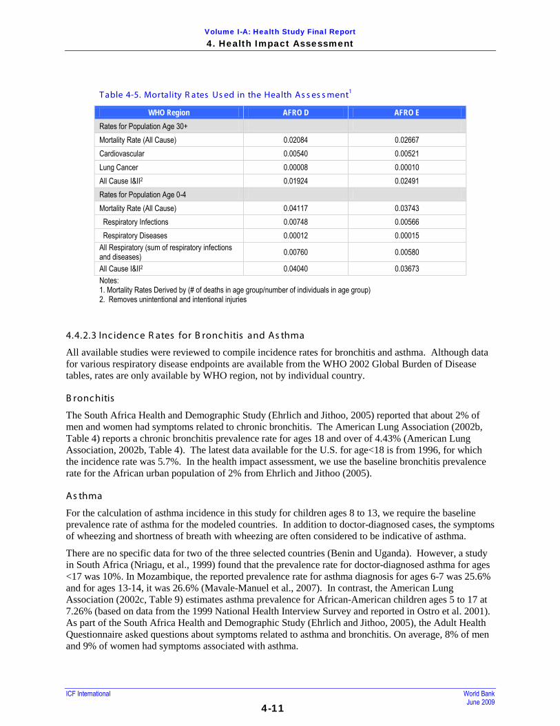
Volume I-A: Health Study Final Report 4. Health Impact Assessment
ICF International World Bank June 2009
4-11
T able 4-5. Mortality R ates Us ed in the Health As s es s ment1
WHO Region AFRO D AFRO E Rates for Population Age 30+ Mortality Rate (All Cause) 0.02084 0.02667 Cardiovascular 0.00540 0.00521 Lung Cancer 0.00008 0.00010 All Cause I&II2 0.01924 0.02491 Rates for Population Age 0-4 Mortality Rate (All Cause) 0.04117 0.03743 Respiratory Infections 0.00748 0.00566 Respiratory Diseases 0.00012 0.00015 All Respiratory (sum of respiratory infections and diseases) 0.00760 0.00580
All Cause I&II2 0.04040 0.03673 Notes: 1. Mortality Rates Derived by (# of deaths in age group/number of individuals in age group) 2. Removes unintentional and intentional injuries
4.4.2.3 Inc idence R ates for B ronchitis and As thma
All available studies were reviewed to compile incidence rates for bronchitis and asthma. Although data for various respiratory disease endpoints are available from the WHO 2002 Global Burden of Disease tables, rates are only available by WHO region, not by individual country.
B ronchitis
The South Africa Health and Demographic Study (Ehrlich and Jithoo, 2005) reported that about 2% of men and women had symptoms related to chronic bronchitis. The American Lung Association (2002b, Table 4) reports a chronic bronchitis prevalence rate for ages 18 and over of 4.43% (American Lung Association, 2002b, Table 4). The latest data available for the U.S. for age<18 is from 1996, for which the incidence rate was 5.7%. In the health impact assessment, we use the baseline bronchitis prevalence rate for the African urban population of 2% from Ehrlich and Jithoo (2005).
As thma
For the calculation of asthma incidence in this study for children ages 8 to 13, we require the baseline prevalence rate of asthma for the modeled countries. In addition to doctor-diagnosed cases, the symptoms of wheezing and shortness of breath with wheezing are often considered to be indicative of asthma.
There are no specific data for two of the three selected countries (Benin and Uganda). However, a study in South Africa (Nriagu, et al., 1999) found that the prevalence rate for doctor-diagnosed asthma for ages <17 was 10%. In Mozambique, the reported prevalence rate for asthma diagnosis for ages 6-7 was 25.6% and for ages 13-14, it was 26.6% (Mavale-Manuel et al., 2007). In contrast, the American Lung Association (2002c, Table 9) estimates asthma prevalence for African-American children ages 5 to 17 at 7.26% (based on data from the 1999 National Health Interview Survey and reported in Ostro et al. 2001). As part of the South Africa Health and Demographic Study (Ehrlich and Jithoo, 2005), the Adult Health Questionnaire asked questions about symptoms related to asthma and bronchitis. On average, 8% of men and 9% of women had symptoms associated with asthma.

Volume I-A: Health Study Final Report 4. Health Impact Assessment
ICF International World Bank June 2009
4-12
For the proportion of children with asthma, and for the baseline prevalence of asthma symptoms, the values used in this health impact assessment are shown in the Table 4-6.
T able 4-6: P revalenc e R ates for As thma Us ed in the Health As s es s ment
Health Endpoint Ages Prevalence Rate Reference As Applied in Health Impact Assessment
Doctor-Diagnosed Asthma <17 10% Nriagu et al., 1999, South Africa
10% - Baseline Asthma Prevalence in Children ages 8-13 for South Africa
Asthma Diagnosis 6-7 and 13-14
26% (ever had asthma)
Mavale-Manuel et al., 2007, Mozambique
26% - Baseline Asthma Prevalence in Children ages 8-13 for Benin and Uganda
Wheezing <17 37% Nriagu et al., 1999 37% - Used for all countries Shortness of Breath with Wheeze <17 16% Nriagu et al., 1999 16% - Used for all countries Chronic Cough <17 35% Nriagu et al., 1999 16% - Used for all countries
4.5 Unc ertainties As s oc iated with the Health Impac t As s es s ment
The uncertainties associated with the health impact assessment include: the selection of the modeled annual average air concentration; the selection of a single pollutant model and a subset of emissions-related health impacts; the studies used to evaluate health impacts; and the accuracy of baseline mortality and illness rates.
Us e of the Annual Average or Average Daily Air C oncentrations as the E xpos ure C oncentrations
Use of the annual average or daily average air concentrations as the exposure concentrations for individuals in urban areas may under-estimate exposures for some of these individuals. Concentrations in various regions of the city could vary widely from the average. For example, those living near major roadways may be exposed to higher annual average concentrations. This approach ignores the peaks in exposure that could occur at different times of the year. The main sources of emissions - domestic fuel burning, road dust, and vehicle emissions - may vary across the modeling domain.
S election of C ertain P ollutants and Health Impacts
Impacts are assessed only for a subset of pollutants and possible health impacts. We focus our study on PM2.5, PM10, and benzene in outdoor air. The health endpoints examined could be associated with other measures of particulate air pollution, such as total suspended particles, or with other types of gaseous pollutants (Pope et al., 2002). In addition, diesel engine emissions have been separately associated with health impacts in some studies, and in the U.S., California’s Environmental Protection Agency (Cal EPA) considers diesel emissions a carcinogen.96
96 In 1998, particulate matter for diesel-fueled engines (diesel PM) was recognized by the California Air Resources Board (ARB) as the toxic air contaminant that best characterized the toxic risk from diesel exhaust. The Cal EPA, Office of Environmental Health Hazard Assessment, recommended a cancer unit risk factor (URF) of 300 excess cancers per million per microgram per cubic meter of diesel PM.
A screening evaluation of the estimated reduction of diesel PM, using the modeled concentrations for Johannesburg, RSA, indicate that, using the Cal EPA unit risk value, there could be a change between the Base Case and Scenario 2 of a net annual average decrease of

Volume I-A: Health Study Final Report 4. Health Impact Assessment
ICF International World Bank June 2009
4-13
about 0.19 μg/m3 region-wide and a peak decrease of about 2.6 μg/m3. Additional analysis of the diesel emissions, therefore, would be an important refinement to this study.
Other air pollution-related health endpoints have been measured in previous studies, such as increased hospital admissions, missed work or school days, and others. These effects were not examined in this study, perhaps leading to an under-estimate of the benefits of switching to lower sulfur fuels.
S tudies Us ed to Quantify Health Impact
Although the studies used to quantify potential health impacts were published in peer-reviewed journals, and have been used in the past as a basis for studying the connection between air pollution and health, there are uncertainties associated with these studies. The authors often consider potential confounders or other risk factors that could account for the observed relationship, but may not have accounted for all of these factors. Risk factors, such as smoking or diet, may be controlled for, but may vary over the time of the study follow-up or may differ according to the location of the population (e.g., urban or rural).
The E-R functions used were developed using data derived at certain air pollution levels. However, it is not known what shape these E-R functions take at higher concentrations, and they may not be appropriate for the air concentrations modeled in this study. In addition, the time frames in the studies may be different than the exposure periods considered in this study. For example, Ostro et al. (2001) looked at the relationship between PM2.5 concentrations and asthma symptoms measured over a 12-hour period, and this study considers these potential health impacts for a 24-hour period.
Using data regarding air pollution health impacts from developed counties is problematic when discussing less developed countries. The E-R functions used in this study, although we feel they are the best available to describe the relationship between PM exposure and health effects, may not be applicable to the populations of the SSA cities under consideration. There are likely to be differences in risk factors; in addition, there are well-documented differences in a variety of measures between different socioeconomic levels. For example, although Pope et al. (2002) consider the interaction of risk factors such as age, sex, smoking status, occupational exposure, diet, and education, and these interactions may or may not have been found to be significant, the occurrence of these risk factors are likely to be different in the SSA populations in this study, or other risk factors not considered in the Pope et al. study may be more relevant to SSA populations. These uncertainties could affect the estimated health benefits due to PM reductions in this study.
It is well known that urban air pollution has a relatively higher impact on the urban poor than on the general population for several reasons:
• The average baseline health status of the poor is often impaired, reducing their resistance to disease and increasing the chances that they will suffer health effects from air pollution;
• Housing of the urban poor is usually low-quality, badly ventilated, and heated by basic systems using fuels and techniques that produce high levels of indoor pollution;
• The urban poor may live in areas close to air pollution sources in industrial or heavily exposed down-wind areas, potentially exposing them to higher concentrations of air pollution than the average city levels.97
97 UNEP Urban Air Quality Management Toolkit

Volume I-A: Health Study Final Report 4. Health Impact Assessment
ICF International World Bank June 2009
4-14
Ac curac y of B as eline Mortality and Morbidity R ates
Databases on mortality and illness are likely to be incomplete, often due to incomplete reporting and statistics-gathering. According to data provided by 112 Member States, the WHO estimates that only about one-third of the estimated 56 million deaths occurring annually are recorded in vital registration systems.

Volume I-A: Health Study Final Report 5. Health Valuation
ICF International World Bank June 2009 5-1
5. Health Valuation The final step of the health study requires information on the value of the health risk reductions associated with decreased pollution exposure, so that the benefits of improvements in air quality can be compared to their costs in monetary terms. The Health Study focuses on quantifying the value of reducing the effects of these pollutants on adult and infant mortality, on the incidence of chronic bronchitis, and on exacerbation of asthma symptoms among children.
This section describes the derivation of monetary values for the quantified health risk reductions that are appropriate for SSA. A full description of the methods used for the health valuation may be found in Appendix F.
5.1 V aluation Approac hes When valuing health risk reductions for benefit-cost analyses, economists generally consider three types of metrics: estimates of willingness to pay (WTP), of monetized quality-adjusted life years (QALYs) or disability-adjusted life-years (DALYs), and of the cost of illness (COI). While WTP is the preferred measure, other measures may be used as rough proxies when relevant studies are not available.
Willingness to Pay: WTP reflects an individual’s willingness to trade his or her own income for health improvements, and is thus the metric most consistent with the types of trade-offs considered in benefit-cost analyses. QALYs and DALYs consider only trade-offs between time spent in different health states, while WTP considers the trade-offs between expending income on health risk reductions or on other goods and services. Thus WTP is more consistent with the benefit-cost analysis framework.
For outcomes that are not directly bought and sold, such as the health risk reductions associated with decreased pollution, WTP is usually estimated from revealed or stated preference studies.
Revealed preference studies rely on data from market transactions or observed behavior to estimate the value of related nonmarketed goods, while stated preference studies generally rely on responses to survey questions. Each approach has advantages and limitations. For example, revealed preference studies have the advantage of relying on data from actual markets, but may address scenarios that differ in significant respects from those of concern in policy analysis. Stated preference studies enable researchers to better tailor the scenario to the risks of concern, but the responses are hypothetical in nature. As a result of these and other concerns, careful review of the underlying studies is needed to determine their quality and applicability.
Monetized Health-Adjusted Life Years: This option involves first estimating the DALY or QALY gains (i.e., the additional years of life or years of good health) associated with reducing the number of cases of illness or injury, then assigning a monetary value to these gains. Both DALYs and QALYs are non-monetary measures that integrate consideration of health-related quality of life over time and longevity, so that a single metric can be used to compare health effects of varying types. These metrics focus on the trade-offs between different health states, represented on a scale anchored at “0” and “1.” Under the QALY approach, “0” represents a state viewed as equivalent to dead and “1” represents perfect or full health. The scale is reversed for DALYs, with “0” representing full health and “1” representing a state equivalent to dead.
Both approaches can be applied in a variety of different ways. However, the most common DALY framework is that implemented by the World Health Organization (WHO), which explicitly incorporates egalitarian principles. WHO’s approach is evolving over time, but generally uses the same values for all
Volume I-A: Health Study Final Report 5. Health Valuation
ICF International World Bank June 2009
5-2
regions of the world, including an ideal life expectancy standard and adjusting only for age and sex. Its approach can also give less weight to those years lived at younger and older ages.
To use QALYs or DALYs in benefit-cost analysis, they must be assigned a monetary value. Often, a constant value per statistical life year (VSLY) is used for this purpose. Recent research indicates, however, that neither theory nor the available empirical research supports a constant VSLY. In addition, a 2006 U.S. Institute of Medicine expert panel recommended against using monetized QALYs or DALYs in benefit-cost analysis because of the inconsistencies in the types of trade-offs assessed and the lack of evidence supporting the monetary values. QALYs and DALYs consider only trade-offs between time spent in different health states, while WTP considers the trade-offs between expending income on health risk reductions or on other goods and services. Thus WTP is more consistent with the benefit-cost analysis framework.
Avoided costs: The COI approach most commonly involves estimating the averted medical costs (direct costs) associated with preventing a case of illness. The value of lost productivity (indirect costs) is often also assessed, including the effects of illness on paid and occasionally unpaid work time (i.e., human capital). Other cost savings, such as those related to insurance administration and litigation, may also be considered.
The COI approach usually understates the value of risk reductions. Perhaps most importantly, COI estimates do not include the value of avoiding pain and suffering nor other impacts on the quality of life. They address an outcome that differs from the outcome of efforts to reduce air pollution or other risks. For example, they reflect the ex post costs associated with actual cases rather than the ex ante value associated with potential risk reductions, and focus on treatment which (unlike prevention) may not return an individual to his or her initial health state. In addition, COI estimates are usually based on the average cost per case, which may differ from the marginal change in resource use or productivity associated with small reductions in the total number of cases.
Given these concerns, this report focuses on deriving estimates of WTP. Because WTP estimates are not available for Sub-Saharan Africa or other low income countries, it extrapolates from estimates developed in countries with higher incomes. While this approach is consistent with that used in previous World Bank studies, the values are revised and refined based on the results of newer research and analysis.
5.2 Mortality R is k R educ tions For mortality risks, analysts usually rely on estimates of the value per statistical life (VSL). A “statistical life” involves aggregating small changes in risks across many individuals. For example, a 1 in 10,000 risk reduction that affects 10,000 individuals can be expressed as a statistical life (1/10,000 risk x 10,000 individuals = 1 statistical life). A statistical life is also equivalent to a 1 in 100,000 risk reduction that affects 100,000 individuals (1/100,000 risk x 100,000 individuals = 1 statistical life). In both cases, eliminating the risk would reduce the expected number of deaths in the respective population by one, but the individual whose life would be extended is not identifiable in advance.
The VSL is typically calculated by dividing individual WTP for a small risk reduction by the size of the risk change. For example, a $50,000 VSL would result if an individual was willing to pay $5 to reduce his or her risk of death by 1 in 10,000 over a specified time period ($5 ÷ 1/10,000 = $50,000). Alternatively, the VSL can be expressed by aggregating WTP across a wider population. A $50,000 VSL would result if each member of a population of 10,000 was willing to pay $5 on average for a 1 in 10,000 annual decrease in risk ($5 x 10,000 = $50,000).
The VSL concept can be controversial because it is frequently misunderstood. It is not the value of saving a “life,” nor is it a measure of the moral worth or inherent value of an individual. Instead, it represents the

Volume I-A: Health Study Final Report 5. Health Valuation
ICF International World Bank June 2009
5-3
rate at which individuals are willing to exchange their own income for a small reduction in their own mortality risk in a particular time period. While this rate is conventionally expressed as WTP per statistical life saved, it could be equally well expressed as WTP for any specified small risk change. As indicated by the examples above, a VSL of $50,000 is the same as a value of $5 for a 1/10,000 risk reduction.
These values reflect an individual’s own preferences, subject to the actual constraints he or she faces. Individuals make decisions that reflect these preferences frequently; for example, by spending more for a safer car, taking a lower risk job for less pay, purchasing helmets or other protective equipment, or choosing more expensive but less hazardous cooking fuel. In each case, the decision to exchange income for increased safety involves foregoing expenditures on other goods and services.
WTP for risk reductions is likely to be smaller among individuals with lower incomes than for higher income individuals, because they face more pressing demands for other expenditures that will improve their well-being, such as food and shelter. Because of this relationship, the VSL will vary across individuals, communities, and countries with different income levels.
5.2.1 V S L L iterature R eview
Most research on the VSL is based on revealed preferences, particularly the trade-off between wages and job-related risks. In these wage-risk studies (also referred to as hedonic wage or compensating wage differential studies), researchers compare earnings across workers in different occupations or industries who face varying levels of on-the-job risks, using statistical methods to control for the effects of other factors (such as education or nonfatal job risks) on wages. An increasing number of studies instead use stated preference methods, such as contingent valuation surveys, to estimate individual WTP for mortality risk reductions in different contexts.
Previous World Bank air pollution studies have relied largely on reviews of the VSL literature completed in the early 1990s that primarily address high income countries. Since that time, five major meta-analyses have been completed that combine the results of several VSL studies. However, the studies included in these analyses rely on relatively old data and do not reflect the evolving research on how to best specify related statistical models. In addition, a recent expert panel review suggested that these meta-analyses are in need of improvement, both in the criteria applied to select studies and in the statistical techniques used when combining the results.
Review of the more recent VSL research for high income countries suggests that the Viscusi (2004) U.S. wage-risk study best represents currently recommended practices. , This study reflects significant improvements in the U.S. data available on job-related fatality risks, and effectively controls for other factors that influence the trade-off between income and risk reductions (such as nonfatal job risks and workers’ compensation for injuries). The best estimate from this study is $4.7 million in 1997 dollars, or $6.3 million in 2007 dollars if adjusted for inflation and real income growth, using rates applicable to the U.S.
The VSL is likely to vary across countries due to differences in income, attitudes towards health risks, and other factors. Thus this report also reviews studies conducted in lower income countries. These include 17 studies (eight wage-risk studies and nine stated preference studies) conducted in nine countries, using data collected between 1982 and 2005. While the populations studied have annual earnings ranging from about $600 to $10,600 (2007 dollars, based on market exchange rates), all of the studies were conducted in countries classified as “middle income” by the World Bank.

Volume I-A: Health Study Final Report 5. Health Valuation
ICF International World Bank June 2009
5-4
In contrast, the 49 African countries included in this study include many of the poorest in the world. When measured by gross national income (GNI) per capita using exchange rates, 2007 average income levels range from a high of about $12,900 in Equatorial Guinea to a low of about $100 in Burundi. If measured instead by purchasing power parity (PPP) per capita, GNI ranges from a high of about $21,200 in Equatorial Guinea to a low of about $300 in the Democratic Republic of the Congo and Liberia. (Within each country, substantial income disparities often exist.) For the entire sub-Saharan region, per capita GNI averages about $1,000 if measured using exchange rates or $1,900 if measured as PPP. In contrast, the U.S. per capita GNI is about $46,000, regardless of whether exchange rates or PPP conversion factors are used.
The 17 studies mentioned above vary in quality, but suggest that the VSL differs significantly across populations with different income levels. The best of these studies indicate that the VSL is roughly 60 to 170 times earnings in these lower income populations. Estimates from the U.S. and other high income countries appear somewhat larger in comparison to earnings. The results from Viscusi (2004) yield a ratio of about 170, and the meta-analysis by Viscusi and Aldy (2003) yields a ratio of about 260. These comparisons often include only wage income, because broader measures of income (such as GNI) are generally calculated on a national basis and are not available for the subpopulations included in many of the studies. The uncertainties associated with using the GNI are discussed further in the uncertainty section of this report.
Further investigation of the relationship between real income and the VSL suggests that this relationship varies. The income elasticity of the VSL (i.e., the percent change in the VSL associated with a one percent change in income) has been studied in a number of different contexts. Most studies conducted in high income countries suggest that the VSL increases at roughly half the rate of income; i.e., that income elasticity is approximately 0.5. However, studies that look at changes over long time periods or across significantly different economies suggest that this elasticity exceeds a value of 1.0 in many cases, in part because of the relationship between economic development and the demand for safety.
5.2.2 V S L R ec ommendations
Review of the 17 studies conducted in middle income countries suggests that there is not yet enough high quality research to rely solely on these studies when developing VSL estimates. However, when combined with other research on the relationship between the VSL and income, these studies support the use of a higher elasticity estimate when extrapolating from VSL studies conducted in high income countries to those with lower incomes, than is used when extrapolating the VSL across high income areas.
Thus for the Sub-Saharan Africa Refinery Study, this report recommends the use of central estimates calculated by applying an income elasticity estimate of 1.5 to the results of the Viscusi (2004) study; i.e., to a U.S. VSL of $6.3 million in 2007 dollars. Because the appropriate elasticity is uncertain, it also recommends reporting the results using a range of values, based on elasticities of 1.0 and 2.0. An elasticity of 1.0 corresponds to the approach used in several previous World Bank studies, while some research suggests that income elasticity may be closer to 2.0 when extrapolating across economies in significantly different states of development. The calculations are based on per capita GNI, since this is the most comprehensive measure of national income available. While conversions based on purchasing power are more representative of actual consumption in lower income countries, the report also presents estimates based on market exchange rates for comparison.
Theory suggests that the VSL should not be less than the present value of future lifetime consumption. Thus this study uses estimates of future consumption as a lower bound for the VSL estimates. Because an elasticity of 2.0 results in the smallest VSL estimates, this approach leads to replacement of these low end estimates with the estimates of future consumption for all but the wealthiest countries. For the poorest

Volume I-A: Health Study Final Report 5. Health Valuation
ICF International World Bank June 2009
5-5
countries, the estimates of future consumption are also greater than the VSL estimates developed using an elasticity of 1.5.
For the entire Sub-Saharan Africa region, this approach results in an average VSL of $51,900, based on purchasing power parity and an income elasticity of 1.5. This central estimate is very uncertain. If an income elasticity of 1.0 is used, the high estimate for the region is a VSL of $256,900. The low estimate is based on future consumption and varies depending on the discount rate: $42,700 with a 3 percent rate or $24,800 with a 7 percent rate.
The highest income country in the region is Equatorial Guinea, with GNI per capita of $21,230 based on purchasing power. In this case, the VSL estimates are not bounded by the estimates of future consumption, and equal $1.4 million with an elasticity of 2.0, $2.0 million with an elasticity of 1.5, and $2.9 million with an elasticity of 1.0. The lowest income countries are the Democratic Republic of the Congo and Liberia, with GNI per capita of $290 and a high VSL estimate of $39,800. The central and low estimates for these countries are based on future consumption: with a 3 percent rate, both the central and low estimates are $6,900; with a 7 percent rate, the central and low estimates are $3,900.
The relatively wide ranges that result indicate the substantial uncertainty in the VSL estimates appropriate for countries in this region. Extrapolating from higher income countries, using the range of elasticities that result from available research, leads to large differences in the resulting VSLs, which in many cases fall below estimates of future consumption. This result may in part indicate that the income elasticity estimates reflect the effects of other factors that are not adequately controlled in the underlying studies, such as differences in cultural attitudes towards mortality risks.
In addition to income, there are a number of other differences between the Viscusi (2004) research and the mortality risks associated with air pollution in Sub-Saharan Africa. These include population characteristics such as age, life expectancy, health status, and total mortality risk. The Viscusi study also focuses on job-related deaths from accidental injuries, while air pollution leads to deaths from illness. However, the available research is not sufficient to support quantitative adjustment of the VSL to reflect these differences, especially given that these characteristics may be viewed differently across countries and cultures.
5.2.3 S elec ted Values for Mortality R is k V aluations
There are a number of differences other than income between the Viscusi (2004) research and the mortality risks associated with air pollution in Sub-Saharan Africa. These include population characteristics such as age, life expectancy, health status, and total mortality risk.98
5.3 Morbidity R is k R educ tions
In addition, the Viscusi study focuses on job-related deaths from accidental injuries, while air pollution leads to deaths from illness. However, the available research is not sufficient to support quantitative adjustment of the VSL to reflect these differences, especially given that these characteristics may be viewed differently across countries and cultures.
In addition to mortality risks, this report considers values for two types of nonfatal health effects: new cases of chronic bronchitis among adults (expressed as statistical cases), and exacerbation of symptoms (coughing, wheezing, or shortness of breath) among asthmatic children (expressed as the probability of a 98 Due to the limitations of the available research, the report recommends using the same values for adults and children, while noting that
mortality risks to children are generally valued more highly. This and other differences are discussed in more detail in Appendix F.

Volume I-A: Health Study Final Report 5. Health Valuation
ICF International World Bank June 2009
5-6
day in which each symptom occurs). The literature review conducted for this report indicates that WTP estimates are now available for these effects that can be adapted for use in the Sub-Saharan Africa Refinery Project. Thus, unlike many previous air pollution studies, this report relies on WTP estimates for valuation rather than rough proxies based on the cost of illness or other measures. The major limitation of these estimates is that they are derived from research conducted in countries with much higher average income levels than those found in Sub-Saharan Africa. Thus the values are adjusted to reflect these lower incomes.
5.3.1 C hronic B ronc hitis
For cases of chronic bronchitis, the literature review yielded three sources of WTP estimates: the approach applied by the U.S. Environmental Protection Agency (USEPA) in its analyses of air pollution regulations, a Japanese study, and a Chinese study. Because of concerns about the limitations of the Japanese and Chinese studies, this report relies on the U.S. estimate of $422,000 per statistical case, despite the fact that it is based on relatively old research (published in 1991 and 1992). To adjust for differences in national income, a central elasticity estimate of 1.5 is used, derived from comparison of the U.S. and Chinese values and the similarity between Chinese and Sub-Saharan African income levels. For high and low estimates, elasticities of 1.0 and 2.0 are applied. Although these elasticities are identical to those used for the VSL estimates, the results are more uncertain due to the very small number of relevant studies.
For chronic bronchitis, this approach leads to a central estimate per statistical case of $3,500 based on GNI per capita for the entire sub-Saharan region if purchasing power parity conversion rates are used. Substituting income elasticity estimates ranging from 1.0 to 2.0 leads to regional estimates ranging from $700 to $17,200.
5.3.2 As thma E xac erbations
For asthma exacerbations, the review considered the US EPA’s current approach (which is based on a study published in 1986), the results of three newer meta-analyses (each of which includes between five and 17 primary research studies), and one study completed too recently to be included in the meta-analyses. Because these values are very small in comparison to the values for chronic bronchitis and mortality risks, this report suggests a relatively simple approach to valuation. Based on the results of the WTP studies, it assumes that the value of a symptom day for each effect is 0.1 percent of income, equivalent to assuming an income elasticity of about 1.0. If these effects occur frequently enough that multiplying even these small values by the number of symptom days averted leads to totals that could noticeably affect the analytic results, then sensitivity analysis can be conducted with higher and lower estimates.
The value per symptom day for asthma exacerbations is much smaller than that for bronchitis, ranging from $1.00 to $2.00 for the region.
5.3.3 S elec ted Values for Morbidity R is k V aluations
For the individual countries, based on purchasing power and an income elasticity of 1.5, the value per statistical case of chronic bronchitis ranges from a high of $133,000 in Equatorial Guinea to a low of about $200 in the Democratic Republic of the Congo and Liberia. The range for the estimates for asthma symptoms is from less than $1.00 to about $20 per symptom day. Thus the large income differences between these countries lead to wide variation in the estimates of average individual WTP for these risk reductions. In addition, factors other than income (such as cultural differences in health risk preferences)

Volume I-A: Health Study Final Report 5. Health Valuation
ICF International World Bank June 2009
5-7
are likely to affect these values. More research would be needed that explicitly addresses mortality and morbidity values in low income countries to reduce the uncertainties in these estimates.
5.4 Unc ertainties As s oc iated with the Health V aluation The income elasticity ranges provided for the mortality and the morbidity valuation estimates, corresponding to the ranges in suggested monetary values for mortality and morbidity, suggest substantial uncertainty in the appropriate estimates for this region; more primary research regarding income elasticity would be needed to narrow this range. In addition, the income elasticity estimates may reflect other factors that are not adequately controlled in the underlying studies, such as differences in cultural attitudes towards mortality risk. In addition, although the elasticities used for VSC for bronchitis are identical to those used for the VSL estimates, they are more uncertain due to the very small number of relevant studies.
The large income differences between the countries in SSA lead to wide variation in the estimates. In addition, within the individual countries of SSA there is enormous income disparity. With the large increases in the prices of oil, gold and other raw minerals, the GDPs of many of the SSA countries, which rely on commodity exports and their export revenue, have escalated rapidly. The past decade has seen the rapid growth of the middle class; nevertheless large numbers of poor people still exist, resulting in an income distribution in which the majority of people are very poor, a small, but growing number are middle class, and a very small percentage are rich. For the Health Study, this means uncertainties are associated with using the GNI for valuing pollution reduction benefits.
In addition, for both mortality and morbidity risk reductions, factors other than income (such as cultural differences in health risk preferences) will affect the valuation estimates. More research would be needed that explicitly addresses mortality and morbidity values in low income countries to reduce the uncertainties in these estimates.

Volume I-A: Health Study Final Report 6. Calculation of Health Impacts and Monetary Benefits
ICF International World Bank June 2009 6-1
6. Calculation of Health Impacts and Monetary Benefits
The calculation of health impacts for each of the health endpoints uses a model relating exposure and potential health impact (response), as described in Section 4.2, along with the monetary valuation of each of the health endpoints (Section 5.0).
The potential health impact, that is, the predicted change in incidence in the population associated with a change in fuel specifications, requires the following inputs (described in previous sections, as noted):
• A baseline rate for the health endpoint (Sections 4.4.2 and 4.4.3)
• The beta (β)99
• Estimates of Base Case and Scenarios 1 and 2 concentrations (Section 4.4.1)
from the exposure-response model (Section 4.2)
• The total population of the city (Section 4.4.2)
• The age distribution of the population (Section 4.4.2)
• The monetary valuation of once case of mortality, bronchitis, and asthma (Sections 5.3 and 5.4)
6.1 E as t R egion
6.1.1 Quantitative C ity E valuation - E as t R egion
For Kampala, the quantitatively evaluated city in the East region, the estimated changes in modeled air concentrations for areas within the modeling domain with greater than 1,000 people/km are discussed in this section. The change in the annual average total PM2.5 concentrations between the Base Case and Scenario 1 (change in fuel specifications only) was 1.71 μg/m3, and for PM10 concentrations, the change was 1.66 μg/m3. Between the Base Case and Scenario 2, the predicted change in PM2.5 concentrations was 5.39 μg/m3, and for PM10 concentrations, the predicted change was 5.18 μg/m3.
These decreases in PM air concentrations correspond to decreases in mortality and morbidity rates and estimated benefits, as shown in Table 6-1. T able 6-1: S ummary of Health S tudy R es ults for the E as t R egion C ity (K ampala, Uganda)
Reduction in Number of Cases
All-Cause Mortality (Ages >30)
Cases of Bronchitis (Ages >30)
New Onset Asthma Exacerbations (Ages 8-13)
Respiratory Disease Mortality (Ages <5)
Scenario 1 510 2500 240 5
Scenario 2 1600 7900 760 10
Notes: Values are rounded. For areas within the modeling domain with greater than 1,000 people/km.
Reductions in the modeled annual average benzene concentrations (from 9.7 μg/m3 in the Base Case, to 6.1 μg/m3 in Scenario 1 and 3.1 μg/m3 in Scenario 2 for areas with population density greater than 1,000/km) correspond to an estimated maximum reduction of less than 150 benzene-related cancer cases.
99 As previously described, the beta (β) is the coefficient of the model, which describes the relationship between the exposure and the health effect.

Volume I-A: Health Study Final Report 6. Calculation of Health Impacts and Monetary Benefits
ICF International World Bank June 2009
6-2
The health benefits due to benzene reductions are small relative to the benefits associated with PM, and thus are not carried though to the regional analysis and are not included in the valuation results.
6.1.2 Qualitative C ity E valuations - E as t R egion
Nairobi, Kenya, and Dar Es Salaam, Tanzania are qualitatively evaluated for the East region. Detailed emissions data were not available for these two cities, thus the Base Case and Scenario 1 emissions are discussed quantitatively.
For Nairobi, the changes in fuel specifications would have the most important effect on reducing benzene concentrations in outdoor air, possibly reducing annual average benzene concentrations by up to a factor of 3. Ambient concentrations of SO2 should show much larger reductions with the introduction of clean fuels than Kampala owing to the much larger fraction of SO2 emissions attributable to motor vehicles. Similar to Kampala, little or no change would be seen in ambient PM2.5 concentrations because a large fraction of PM2.5 results from domestic sources. A corresponding small monetary benefit would be calculated based on this result.
Similar to Kampala and Nairobi, in Dar Es Salaam, it is anticipated that the change in fuel specifications would have the most important effect on reducing benzene concentrations, probably reducing annual average benzene concentrations by up to a factor of 3. Ambient concentrations of SO2 should show much larger reductions in Dar Es Salaam compared to Kampala, because of the much larger fraction of SO2 emissions attributable to motor vehicles. Similar to Kampala, little to no change would be seen in ambient PM2.5 concentrations owing to the large fraction of PM2.5 concentrations from re-entrained road dust and domestic sources of open air burning of household wastes, wood, and charcoal. Note that somewhat lower ambient PM concentration levels are anticipated for Dar Es Salaam compared to Kampala owing to its coastal location with generally higher annual average wind speeds (i.e., better air mixing). Correspondingly, lower health and monetary benefits would accrue in this city.
6.1.3 R egional Analys is - E as t R egion
The East region results for Scenario 2 using the alternate assumptions are presented in Table 6-2. The regional results are based on an extrapolation from the air modeling for Kampala. The table shows the reduction in the number of cases, the annual estimated dollar benefit, and the five-year and ten-year benefits associated with the reduction in cases.

Volume I-A: Health Study Final Report 6. Calculation of Health Impacts and Monetary Benefits
ICF International World Bank June 2009
6-3
T able 6-2: Health S tudy E as t S S A R egional Analys is R es ults Us ing Alternate 2-S troke Motorcyc le As s umptions
East Region -
Number of Cases of:
All-Cause Mortality - Reductions in PM2.5 (ages>30)
Bronchitis Cases - Reductions in PM2.5 (ages>30)
Asthma Exacerbations - Reductions in PM10 (ages 8-13)
Respiratory Disease Mortality - Reductions in PM10 (ages<5)
Estimated Total Annual
Benefit (million 2007 US dollars)2
Estimated Five-Year
(NPV) Benefit (billion 2007 US dollars)2,3
Estimated Ten-Year
(NPV) Benefit (billion 2007 US dollars)2,3
Base Case 541,823 2,293,281 3,183,871 12,050 -- --
Scenario 1 532,449 2,247,042 3,179,640 12,001 $340 M
($160 M; $2,000 M)
$1.4 B ($0.66 B;
$8.2 B)
$2.4 B ($1.1 B;
$14 B)
Scenario 2 506,516 2,118,796 3,167,322 11,862 $1,300 M ($610 M;
$7,500 M) $5.3 B ($2.5
B; $31 B)
$9.0 B ($4.3 B;
$53 B) Notes: 1. Using air modeling concentrations for >1,000 population density within each quantitatively evaluated city, extrapolated to the region, and using alternate 2-stroke motorcycle assumptions for Scenario 2. 2. Dollar benefits shown are those using alternate 2-stroke motorcycle assumptions for Scenario 2 and that apply the country-specific VSL or VSC, elasticity of 1.5, and GNI using PPP. The dollar values in parentheses show the range from low estimated values (using an income elasticity of 2.0) to high estimated values (using an elasticity of 1.0). 3. Net present values calculated with 7% discount rate.
6.2 Wes t R egion
6.2.1 Quantitative C ity E valuation - Wes t S S A R egion
The results for the west SSA region, based on the quantitatively evaluated city of Cotonou, Benin, are summarized below and in Table 6-3.
For Cotonou, the estimated change in modeled annual average total PM2.5 concentrations for areas within the modeling domain with greater than 1,000 people/km for Scenario 1 (change in fuel specifications only) was 3.81 μg/m3, and for PM10 concentrations, the change was 4.21 μg/m3. For Scenario 2, the changes were much larger, based on the elimination of 2-stroke engines: 88.59 μg/m3 for PM2.5 concentrations and 98.41 μg/m3 for PM10 concentrations. These reductions in PM correspond to decreases in mortality and morbidity rates and estimated US dollar values, as shown in Table 6-3. T able 6-3: S ummary of Health S tudy R es ults for the W es t S S A R egion C ity (C otonou, B enin)
Reduction in Number of Cases
All-Cause Mortality (Ages >30)
Cases of Bronchitis (Ages >30)
New Onset Asthma Exacerbations PM10
(Ages 8-13)
Respiratory Disease Mortality (Ages <5)
Scenario 1 960 50 60 5
Scenario 2 18,000 1,400 2,100 80
Notes: Values are rounded. For areas within the modeling domain with greater than 1,000 people/km.
Reductions in the modeled annual average benzene concentrations (from 161.1 μg/m3 in the Base Case, to 78.3 μg/m3 in Scenario 1 and 6.4 μg/m3 in Scenario 2 for areas with population greater than 1,000/km) correspond to an estimated maximum reduction of about 1,000 benzene-related cancer cases. The health

Volume I-A: Health Study Final Report 6. Calculation of Health Impacts and Monetary Benefits
ICF International World Bank June 2009
6-4
benefits due to benzene reductions are not carried though to the regional analysis and are not included in the valuation results.
6.2.2 Qualitative C ity E valuations - Wes t S S A R egion
Ouagadougou, Burkina Faso and Lagos, Nigeria, are qualitatively evaluated for the West region. Detailed emissions data were available for these two cities, thus changes in emissions from the Base Case to Scenario 1 (change in fuel specifications) are discussed quantitatively. The quantitative evaluation of the change in emissions for Ouagadougou shows a decrease of about 37% in PM emissions, a decrease of about 93% for SOx emissions, and a decrease of about 52% for benzene. These changes compare to a reduction in Cotonou of about 87% for PM emissions, and similar reductions for SOx and benzene.
In Lagos, the population is approximately 9.4 times larger than that of Cotonou, in an area nearly 8 times as large, and has an average population density of at least 17 percent greater than that of Cotonou. The vehicle profiles of Lagos and Cotonou are substantially different; Cotonou has a sizable number of 2-stroke motorcycles, while the vehicle fleet in Lagos contains many more passenger vehicles than Cotonou. However, only approximately 5 percent of trips are made via private car, with 82 percent of trips being made via either minibus or large bus. However, although the total emissions are estimated to be much greater in Lagos than in Cotonou, the predicted emissions reductions for a change in fuel specifications are similar.
6.2.3 R egional Analys is - Wes t S S A R egion
The regional analysis for the west SSA region for Scenario 2 is presented in Table 6-4. The regional results are based on an extrapolation from the air modeling for Cotonou. The table shows the reduction in the number of cases, and the annual estimated benefit and the five-year and ten-year benefits associated with the reduction in cases. T able 6-4: Health S tudy Wes t S S A R egional Analys is R es ults Us ing Alternate 2-S troke Motorcyc le As s umptions
West SSA Region - Number of Cases
of:
All-Cause Mortality - Reductions in PM2.5 (ages>30)
Bronchitis Cases - Reductions in PM2.5 (ages>30)
Asthma Exacerbations - Reductions in PM10 (ages 8-13)
Respiratory Disease Mortality - Reductions in PM10 (ages<5)
Estimated Total Annual Benefit (million 2007 US dollars)2
Estimated Five-Year (NPV) Benefit (billion 2007 US dollars)2,3
Estimated Ten-Year (NPV) Benefit (billion 2007 US dollars)2,3
Base Case 1,325,880 7,387,399 7,464,977 69,140 -- -- --
Scenario 1 1,316,489 7,334,697 7,462,041 69,006 $640 M
($300 M; $3100 M)
$2.6 B ($1.2 B;
$13 B)
$4.5 B ($2.1 B;
$22 B)
Scenario 2 1,249,046 6,952,170 7,444,698 68,238 $4,500 M
($2,000 M; $21,000 M)
$18 B ($8 B; $87 B)
$32 B ($14 B; $150 B)
Notes: 1. Using air modeling concentrations for >1,000 population density within each quantitatively evaluated city, extrapolated to the region, and using alternate 2-stroke motorcycle assumptions for Scenario 2. 2. Dollar benefits shown are those using alternate 2-stroke motorcycle assumptions for Scenario 2 and that apply the country-specific VSL or VSC, elasticity of 1.5, and GNI using PPP. The dollar values in parentheses show the range from low estimated values (using an income elasticity of 2.0) to high estimated values (using an elasticity of 1.0). 3. Net present values calculated with 7% discount rate.

Volume I-A: Health Study Final Report 6. Calculation of Health Impacts and Monetary Benefits
ICF International World Bank June 2009
6-5
6.3 S outh S S A R egion
6.3.1 Quantitative C ity E valuation - S outh S S A R egion
No changes were seen in the annual average concentrations of PM with Scenario 1, due to the overwhelming influence of roadway dust and area sources in Johannesburg and because it was assumed that no 2-stroke motorcycles are in use currently in this city. However, using the assumptions in Scenario 2, that pollution control equipment would be used, led to a decrease in the estimated number of cases of disease.
For Johannesburg, the estimated change in modeled annual average total PM2.5 concentrations for areas within the modeling domain with greater than 1,000 people/km for Scenario 2 were 0.47 μg/m3 for PM2.5 concentrations and 0.46 μg/m3 for PM10 concentrations. These reductions in PM correspond to decreases in mortality and morbidity rates and estimated US dollar values, as shown in Table 6-5. T able 6-5: S ummary of Health S tudy R es ults for the S outh S S A R egion C ity (J ohannes burg, S outh Africa)
Reduction in Number of Cases
All-Cause Mortality (Ages >30)
Cases of Bronchitis (Ages
>30)
New Onset Asthma Exacerbations
(Ages 8-13)
Respiratory Disease Mortality (Ages <5)
Scenario 1 0 0 0 0
Scenario 2 60 100 360 2
Notes: Values are rounded. For areas within the modeling domain with greater than 1,000 people/km. Reductions in the modeled annual average benzene concentrations (from 2.2 μg/m3 in the Base Case, to 1.1 μg/m3 in Scenario 1 and 0.12 μg/m3 in Scenario 2) correspond to an estimated maximum reduction of less than 50 benzene-related cancer cases. The health benefits due to benzene reductions are not carried though to the regional analysis and are not included in the valuation results.
6.3.2 Qualitative C ity As s es s ment - S outh S S A R egion
Cape Town, South Africa, and Maputo, Mozambique, were evaluated qualitatively, with comparisons to the Johannesburg quantitative modeling. We predict that many of the emissions from mobile sources would be lower in Cape Town than in Johannesburg. Mobile source PM2.5 emissions are similar between Cape Town and Johannesburg; however the much lower PM emissions for industry and domestic sources for Capetown would be likely to result in lower annual average PM concentrations in Cape Town. Since there have been dramatic changes in the diesel sulfur content in Capetown since 2001 (diesel fuel oil has dropped from 3,000 ppm to 500 ppm), this would likely correspond to a reduction in SO2 concentrations making the SO2 from motor vehicles more in line with Johannesburg. Overall, SO2 concentrations should be substantially lower than seen for Johannesburg due to significantly less industrial and domestic emissions. For NO2, significantly lower concentrations are likely for Cape Town than Johannesburg due to the lower overall NOx emissions, due to the lower domestic emissions in Cape Town. Benzene concentrations will likely be similar to or slightly less than those found in Johannesburg considering the slightly lower VKT but similar fuel characteristics. However, the generally better mixing of air near the coast may lower concentrations, while inland concentrations may be higher particularly during periods of poor mixing, low wind speeds, and stable atmospheric conditions.

Volume I-A: Health Study Final Report 6. Calculation of Health Impacts and Monetary Benefits
ICF International World Bank June 2009
6-6
The estimated emissions from Cape Town and from Johannesburg are both far greater than those of Maputo, Mozambique, also qualitatively evaluated. This is because of Maputo’s location on the coast, and because of its much lower number of vehicles and VKT.
6.3.3 R egional Analys is - S outh S S A R egion
The regional analysis for the South region for Scenario 2 is presented in Table 6-6. The regional results are based on an extrapolation from the air modeling for Johannesburg, based on the air concentrations in areas populated with greater than 1,000 people/km. The table shows the reduction in the number of cases, and the annual estimated dollar benefit and ten-year benefit associated with the reduction in cases. T able 6-6: Health S tudy S outh R egion Analys is R es ults 1
South SSA Region -
Number of Cases of:
All-Cause Mortality - Reductions in PM2.5 (ages>30)
Bronchitis Cases - Reductions in PM2.5 (ages>30)
Asthma Exacerbations - Reductions in PM10 (ages 8-13)
Respiratory Disease Mortality - Reductions in PM10 (ages<5)
Estimated Total Annual Benefit (million 2007 US dollars)2
Estimated Five-Year (NPV) Benefit (billion 2007 US dollars)2,3
Estimated Ten-Year (NPV) Benefit (billion 2007 US dollars)2,3
Base Case 3,636 108,256 799,209 970 -- -- -- Scenario 1 3,636 108,256 799,209 970 $0 $0 $0
Scenario 2 3,261 107,576 796,852 948 $250 M
($120 M; $550 M)
$1.0 B ($0.45 B;
$2.2 B)
$1.8 B ($0.83 B;
$3.9 B) Notes: 1. These results use the air modeling concentrations for >1,000 population density within each city, extrapolated to the region, for Scenario 2. 2. Dollar benefits shown are those using alternate 2-stroke motorcycle assumptions for Scenario 2 and that apply the country-specific VSL or VSC, elasticity of 1.5, and GNI using PPP. The dollar values in parentheses show the range from low estimated values (using an income elasticity of 2.0) to high estimated values (using an elasticity of 1.0). 3. Net present values calculated with 7% discount rate.
6.4 S ummary of S tudy Unc ertainties Scenario Development
Most countries in SSA do not have specific emission standards or any means to enforce them. Therefore, a major uncertainty is the assumption for Scenario 2 that vehicles will be required to have pollution control equipment, and that a functional inspection and maintenance program will be in place. Implementation of an inspection and maintenance program is not a simple task. There must be the political will to pass such a regulation. Once a regulation requiring pollution control equipment is passed, it will take time to set up an infrastructure sufficient to inspect and maintain the pollution control equipment over time. And, there are costs associated with setting up such a program. Anecdotal evidence indicates that it may take at least 20 years to implement a working program. Any additional regulation regarding a limit on the age of vehicles imported into a country would be another political hurdle. In addition, for Scenario 2, we assume, perhaps optimistically, that 80% of all cars will have functioning pollution control equipment.
Air Modeling
As discussed in Section 3, there are numerous uncertainties associated with the emissions inventory used in the air modeling. However, the World Bank, the ARA Steering Committee, and the study team felt that using actual city-specific data was preferable to estimating these inputs. For example, our use of a percentage of VKT on paved roads of greater than 90% for Cotonou is based on published data from

Volume I-A: Health Study Final Report 6. Calculation of Health Impacts and Monetary Benefits
ICF International World Bank June 2009
6-7
Benin; this value may seem somewhat counter-intuitive, because a much smaller percentage of roads (about 50%) in the city are paved, however, the paved roads carry a much higher fraction of traffic.
As a country’s GNP increases, the number of cars in the country is likely to increase and, possibly, newer cars will be in use. In addition, more roads may become paved, reducing the impact of road dust on airborne PM concentrations. Another potential impact of increasing GNP may be the decreased use of biomass for fuel, as more households use electric or gas stoves. These possible future impacts on emissions and ambient air concentrations were not quantified in this study.
The use of the alternate scenario, in which motorcycle use is assumed to have increased in the West SSA region and decreased in the East SSA region, is not based on quantitative data with regard to current motorcycle activity levels in those regions.
Another uncertainty is associated with the identification of industrial and area sources, based on publicly available databases and publications. There may be additional industrial or area sources that were not identified, and thus were not considered in the emissions and air modeling.
There are uncertainties associated with the city-specific monitoring data that we have used as a comparison to our modeled data. Monitoring data are sparse, and may not represent actual ambient measurements in those urban areas.
It should be noted that the uncertainties associated with the emissions inventory and air modeling are not likely to affect the incremental changes in the ambient concentrations, which are the focus of this study.
Health Impact Assessment
The use of the annual average exposure concentrations to calculate risk may be under-estimate risk for some areas of the cities, as individuals who live closer to roadways or other emissions sources may be more exposed to air pollutants than the average over the whole urban area. In addition, some individuals may be more often exposed to concentrations near the maximum modeled daily concentration than other individuals. Future refinements of this study could include analyses of the highest grid cell concentrations, or estimates of the average pollutant concentrations in the most highly populated regions of each city.
The limitation of this study to selected health endpoints for a limited number of air pollutants may under-estimate the benefits associated with air pollution reductions. However, as discussed in Section 4, we have selected well-documented health endpoints and peer-reviewed studies that associated these health endpoints with particular air pollutants. Many published studies indicate that PM may be the component of the most health concern for exposed individuals; our analyses use the key studies and use the same measure of exposure (namely, PM2.5 for mortality, and PM2.5 and PM10 for some of the morbidity endpoints).
Scaling to a regional level by population assumes same baseline rate of disease, the same mix of emissions sources, similar meteorological and geological characteristics, as well as other factors, resulting in the same decrease in air concentrations from Base Case to Scenario 1 and Scenario 2. This is likely an over-simplification of the actual conditions that certainly vary from one urban area in Sub-Saharan Africa to another. In addition, the consideration of only urban areas with greater than 300,000 population may under-estimate risks and benefits by leaving out smaller urban areas that would also benefit from improved fuels.
We have discussed the issues associated with extrapolating health studies conducted in developed countries to the less-developed countries of SSA. Differences exist with respect to baseline health issues and air pollutant exposure levels. Our use of baseline health data from the countries under study (although potentially incomplete) address some of these issues, however, as stated by Ostro (2004), the
Volume I-A: Health Study Final Report 6. Calculation of Health Impacts and Monetary Benefits
ICF International World Bank June 2009
6-8
slope of the exposure-response function may actually be different in African populations and it may be different at some of the higher exposure levels modeled. Without further study of these relationships for the specific countries in this study, the possible impacts of these issues on the study results are uncertain.
Health Valuation
The major limitation of the estimates of monetary values for mortality and morbidity in the Health Study is that these estimates are based on research conducted in countries with different average income levels than those found in SSA. The VSL100
is likely to vary across countries due to differences in income, attitudes towards health risks, and other factors. Thus, we also reviewed studies conducted in lower income countries. Our research suggested that the VSL differs significantly across populations with different income levels, but that there is not yet enough high quality research to rely on these studies when developing VSL estimates. However, these studies supported the use of a higher elasticity estimate when extrapolating from VSL studies conducted in high income countries to those with lower incomes.
The morbidity values used in this study are also adjusted to reflect lower incomes. For both mortality and morbidity risk reductions, factors other than income (such as cultural differences in health risk preferences) are likely to affect the values. More research would be needed that explicitly addresses mortality and morbidity values in low income countries to reduce the uncertainties in these estimates.
The large income differences between the countries in SSA lead to wide variation in the valuation estimates. In addition, within the individual countries of SSA there is enormous income disparity. The past decade has seen the rapid growth of the middle class; nevertheless large numbers of poor people result in an income distribution in which the majority of people are very poor, a small, but growing, number are middle class, and a very small percentage are rich. As a result, there are uncertainties associated with using the GNI for analysis of pollution reduction benefits.
100 To summarize the text in Section 5, the VSL is not the value of saving a particular individual’s life and it has no implications for the inherent worth of an individual. Rather, it reflects individuals’ WTP to reduce
mortality risk in a specified time period, in cases where the risk reduction is small and the individual whose death would be averted cannot be identified in advance. People with lower incomes are expected to have smaller WTP to reduce mortality risk than higher income individuals, because they face more pressing demands for other expenditures (e.g., food, shelter). VSL is a measure of the rate at which individuals are willing to pay to reduce current mortality risk, thereby forgoing expenditures on other goods and services.

Volume I-A: Health Study Final Report 7. Health Study Summary and Discussion
ICF International World Bank June 2009 7-1
7. Health Study Summary and Discussion
In this Health Study, three scenarios were developed: (1) a Base Case; (2) Scenario 1, based on the implementation of AFRI-4 fuel specifications (gasoline: 150 ppm sulfur, 1 percent benzene; diesel: 50 ppm sulfur), that is, no adjustments were made for increased VKT, increased number of vehicles, changes in vehicle technology, or fleet fuel fraction; and (3) Scenario 2, reflecting a change to AFRI-4 fuel specifications, along with the use of vehicle control technology enabled as a result of having available cleaner fuels, primarily from the reduced sulfur content in both gasoline and diesel, as well as lower benzene levels. Scenario 2 assumes that 80 percent of all vehicles (both public and private) have working vehicle emission control technology; the remaining 20 percent of vehicles were assumed to have older vehicle emission control technology not requiring the use of AFRI-4 fuel specifications. Three cities, representing SSA East, West, and South regions, were modeled quantitatively, and an additional six cities were discussed qualitatively.
In general, small decreases in annual average PM emitted over the whole modeling domain are indicated in the model with the implementation of lower sulfur fuels (Scenario 1), primarily because of the large contribution of roadway dust and domestic sources to overall outdoor PM concentrations in the modeled cities. The decreases vary by region and city based on several key assumptions, including the amount of industry, the percentage of the population using biofuels, and the number of 2-stroke motorcycles and diesel trucks being used. Although the decreases in annual average concentrations of PM associated with the improved fuel specifications appear small, the associated health benefits may be large, as estimated for all-cause mortality in this study. In addition, the decrease in benzene emissions is much larger, potentially reducing vehicle emissions related cancer incidence. Concentrations of other air pollutants emitted, but not included in this model, would also be substantially decreased, in particular with the addition of pollution control equipment in Scenario 2. Differences in the model results across the three quantitatively evaluated cities are based on the variations in emissions inventories for the cities as summarized in Tables 7-1 through 7-4.
T able 7-1: K ey As s umptions for the Development of E mis s ions Inventories , B as e C as e
Key Assumption City Cotonou, Benin Kampala, Uganda Johannesburg , RSA
Population 875,763 1,883,298 2,850,509
City Domain Area 96 sq km 784 sq km 2,304 sq km
Modeling Domain Parameters Geographic Coordinate System WGS_1984_UTM_31N WGS_1984_UTM_36N WGS_1984_UTM_35S Meteorological Grid SW Corner X=425.163 Y=698.387 X=420.025 Y=3.336 X=537.733 Y=7,034.493 Meteorological Modeling Extent (No. cells) 16 E-W x 9 N-S 30 E-W x 30 N-S 56 E-W x 61 N-S Meteorological Modeling Resolution 2-km 2-km 2-km Air Quality Grid SW Corner X=429.163 Y=701.387 X=436.025 Y=19.336 X=579.733 Y=7,070.493 Air Quality Modeling Extent (No. cells) 16 E-W x 6 N-S 14 E-W x 14 N-S 18 E-W x 32 N-S Air Quality Modeling Resolution 1-km 2-km 2-km

Volume I-A: Health Study Final Report 7. Health Study Summary and Discussion
ICF International World Bank June 2009
7-2
T able 7-1: K ey As s umptions for the Development of E mis s ions Inventories , B as e C as e
Key Assumption City Cotonou, Benin Kampala, Uganda Johannesburg , RSA Industrial Description Light Light to Medium Heavy
Industrial Facilities Explicitly Included
3 Small Palm Oil Factories 1 Large Cement Plant 1 Brewery 1 Bottling Facility 1 Shrimp Processing Plant
Uganda Breweries MAKSS Packaging 3 Abbatoirs (slaughterhouses) Sembule Steel
Kelvin Power Carletonville Power Pretoria West Power Johannesburg City Power Durban Road Power John Ware Power Cottesloe Power Lethabo Power Cape Gate Steel Scaw Metals Group Sasol-Natref Refinery Melcast Metalwork
Industrial Facilities Not Explicitly Included None None Equal to 50 percent of Industrial Point Emissions; allocated evenly to identified industrial areas
Industrial Fuel Use
Base: 38,000 tons diesel (4 percent Sulfur); 30,000 tons RFO (Unknown Sulfur Content)
2.2 million gallons RFO (5 percent Sulfur)
5.3 million tons Coal (0.6 to 1.2 percent Sulfur)
Marine Activity Heavy Light None
Marine Vessel Calls (Hotel and maneuver operations only)
410 Carry Containers 224 Roll on/roll off 155 Conv. Cargo 56 Refrig. Ships 103 Petro. Tankers 94 Other Tankers 30 Bulk Carriers 402 Trawlers 80 Other
None None
Domestic Cooking Fuel Charcoal and wood Charcoal and wood Coal
Usage Rates 1,739,900 tons wood 147,000 tons charcoal
281,741 tons wood 300,000 tons charcoal
531,830 tons coal
Spatial Distribution By Population By Population
By Population, Restricted to Heavy and Moderate Coal Burning Areas; Other Areas Assumed to Use Electricity Only

Volume I-A: Health Study Final Report 7. Health Study Summary and Discussion
ICF International World Bank June 2009
7-3
T able 7-1: K ey As s umptions for the Development of E mis s ions Inventories , B as e C as e
Key Assumption City Cotonou, Benin Kampala, Uganda Johannesburg , RSA
Vehicle Fleet Inputs
Fuel Sulfur Levels Gasoline – 600 ppm S Diesel – 5,000 ppm S
Gasoline – 600 ppm S Diesel – 5,000 ppm S
Gasoline – 300 ppm S Diesel – 500 ppm S
Fuel (Gasoline Only) Benzene Levels 3 percent 3 percent 3 percent
Control Technology None None None
Inspection and Maintenance (I/M) None None None
Vehicle Age 15 years 12 years 10.5 years
Vehicle Count (percent VKT) [D = Diesel, P = Petrol]
49,669 P pass. veh. (18 percent) 9,030 D pass. Veh. (13 percent) 13,480 P trucks (7 percent) 7,242 D trucks (4 percent) 35,042 P 4-stroke moto (10 percent) 158,720 P 2-stroke moto (48 percent)
45,470 P pass. veh. (35 percent w/ 4WD) 33,954 P pickups/4WD (35 percent w/ cars) 15,781 D minibus (41 percent) 677 D bus (0 percent) 12,898 D trucks (4 percent) 64,070 P 2-stroke moto (20 percent)
928,174 P pass. veh. (75 percent) 6,771 D pass. veh. (1 percent) 38,767 P minibus (4 percent) 242 D minibus (0 percent) 7,231 D bus (1 percent) 27,932 D light trucks (2 percent) 161,306 P light trucks (13 percent) 29,577 D heavy trucks (4 percent) 0 P moto (0 percent)
Total VKT 4,945 million 798 million 24,700 million
% VKT on paved roads % VKT on unpaved roads Total
95 percent 5 percent
100 percent
94 percent 6 percent
100 percent
99 percent 1 percent
100 percent % VKT from diesel vehicles % VKT from gasoline vehicles Total
17 percent 83 percent 100 percent
45 percent 55 percent 100 percent
8 percent 92 percent 100 percent
% VKT from 2-stage motorcycles % VKT from 4-stage motorcycles % VKT from 4-wheeled vehicles Total
48 percent 10 percent 42 percent 100 percent
20 percent 0 percent 80 percent 100 percent
0 percent 0 percent
100 percent 100 percent

Volume I-A: Health Study Final Report 7. Health Study Summary and Discussion
ICF International World Bank June 2009
7-4
T able 7-1: K ey As s umptions for the Development of E mis s ions Inventories , B as e C as e
Key Assumption City Cotonou, Benin Kampala, Uganda Johannesburg , RSA
Road Dust Factors
PM10 Emission Factor for Unpaved Roads, all vehicles 0.254 kg/km 0.254 kg/km 0.254 kg/km
PM2.5 Emission Factor for Unpaved Roads, all vehicles 0.0253 kg/km 0.0253 kg/km 0.0253 kg/km
PM10 Emission Factor for Paved Roads, cars and trucks 0.0042 kg/km 0.0042 kg/km 0.0042 kg/km
PM10 Emission Factor for Paved Roads, motorcycles 0.0000 kg/km 0.0000 kg/km n.a.
PM2.5 Emission Factor for Paved Roads, cars and trucks 0.0006 kg/km 0.0006 kg/km 0.0006 kg/km
PM2.5 Emission Factor for Paved Roads, motorcycles 0.00035 kg/km 0.00035 kg/km n.a.
T able 7-2: K ey C hanges for the Development of S c enario 1 E mis s ions Inventory as C ompared with B as e C as e
Key Assumption City
Cotonou, Benin Kampala, Uganda Johannesburg , RSA
Industrial Emissions
Industrial Fuel Use Conversion to 100 percent diesel fuel No change No change
Vehicle Fleet Inputs
Fuel Sulfur Levels Petrol – 50 ppm S Diesel – 50 ppm S
Petrol –50 ppm S Diesel – 50 ppm S
Petrol – 50 ppm S Diesel – 50 ppm S
Fuel (Petrol Only) Benzene Levels 0.5 percent 0.5 percent 0.5 percent

Volume I-A: Health Study Final Report 7. Health Study Summary and Discussion
ICF International World Bank June 2009
7-5
T able 7-3: K ey C hanges for the Development of S c enario 2 E mis s ions Inventory as C ompared with S cenario 1
Key Assumption City
Cotonou, Benin Kampala, Uganda Johannesburg , RSA
Industrial Emissions
Industrial Fuel Use No change No change No change
Vehicle Fleet Inputs
Control Technology
80 percent have EURO-III technology vehicles for gasoline or EURO-IV technology vehicles for diesel; 20 percent have none
80 percent have EURO-III technology vehicles for gasoline or EURO-IV technology vehicles for diesel; 20 percent have none
80 percent have EURO-III technology vehicles for gasoline or EURO-IV technology vehicles for diesel; 20 percent have none
Total VKT 5,934 million 958 million 29,640 million
% VKT on paved roads % VKT on unpaved roads Total
95 percent 5 percent
100 percent
94 percent 6 percent
100 percent
99 percent 1 percent
100 percent % VKT from diesel vehicles %VKT from gasoline vehicles Total
17 percent 83 percent 100 percent
45 percent 55 percent 100 percent
8 percent 92 percent 100 percent
% VKT from 2-stage motorcycles % VKT from 4-stage motorcycles % VKT from 4-wheeled vehicles Total
0 percent 58 percent 42 percent 100 percent
0 percent 20 percent 80 percent 100 percent
0 percent 0 percent
100 percent 100 percent

Volume I-A: Health Study Final Report 7. Health Study Summary and Discussion
ICF International World Bank June 2009
7-6
T able 7-4: Indus trial S ources
Facilities Pollutants
SOx (t/y) NOx (t/y) PM10 (t/y) PM2.5 (t/y)
Cotonou (Totala) 1,199 235 120 108
Palm Oil Plant 1 120 24 12 11 Palm Oil Plant 2 120 24 12 11 Palm Oil Plant 3 120 24 12 11 Cement Plant 360 71 36 32 Brewery 240 47 24 22 Bottling Plant 180 35 18 16 Shrimp Processing Plant 60 12 6 5
Kampala (Totala) 793 55 10 9
Uganda Breweries 406 28 5 5 Makss Packaging Industries 247 17 3 3 Uganda Meat Industries 46 3 1 1 Kampala City Council Abattoir 46 3 1 1 Kisita Young Farmers Cooperative Society Abattoir 46 3 1 1 Sembule Steel 2 0 0 0
Johannesburg (Totala) 20,811 53,934 4,901 2,334
Kelvin Power (sum of 5 stacks) 7,872 3,798 121 60 Carletonville Power 79 38 1 1 Pretoria West Power (sum of 2 stacks) 2,125 1,025 33 16 Johannesburg City Power 79 38 1 1 Durban Road Power 79 38 1 1 John Ware Power 79 38 1 1 Cottesloe Power 79 38 1 1 Lethabo Power (sum of 6 stacks) 4,865 46,943 4,413 1,961 Cape Gate Steel 341 165 5 3 Scaw Metals Group 45 22 1 0 Sasol Natref Refinery 5,164 1,790 322 290 Melcast Foundry 5 2 0 0
a. Sum of included facilities may not equal displayed value due to rounding.
The uncertainties associated with this study, as discussed throughout the report, could result in under-estimates of the potential health benefits. For example, this study did not quantify the health and monetary benefits of reductions in sulfur dioxide emissions separately from the benefits of PM reductions, thus perhaps underestimating the overall benefits associated with Scenarios 1 and 2. The selection of a limited number of potential health endpoints may also result in an under-estimate of the potential benefits. In addition, the monetary benefit is based on a willingness-to-pay estimate that may or may not actually apply to the SSA populations under consideration, as discussed in Section 5.

Volume I-A: Health Study Final Report 7. Health Study Summary and Discussion
ICF International World Bank June 2009
7-7
For the East region, as modeled for the city of Kampala, Uganda, the results show a small change in annual average PM concentrations, with valuation numbers smaller than those predicted for the West region city of Cotonou (for all-cause mortality for the population over age 30, $US 3 million for Scenario 1 and $US 9 million for Scenario 2). PM is only marginally affected in this city, since emissions are dominated by roadway dust and domestic sources. The modeling results indicate a larger percentage change in benzene emissions, with the annual average benzene concentrations reduced from 5.6 µg/m3 in the Base Case, to 3.5 and 1.8 µg/m3
for Scenario 1 and Scenario 2, respectively. For Scenario 1, the annual average SO2 concentration is reduced from 1.8 to 0.5µg/m3
(that is, with fuel specification changes only). NO2 concentrations for Scenario 2 are reduced in proportion to the small change in emissions of this compound seen over the Base Case.
In the West region, as represented by the city of Cotonou, Benin, the estimated change in the annual average total PM for Scenario 2 is associated with an estimated decrease annually of close to 6,000 cases of mortality in the population over age 30, with a valuation of about $US 180 million. A decrease of about 50 cases of childhood mortality, with a valuation of $US 1.5 million, is estimated as associated with the decrease in PM2.5 concentrations. A decrease in the number of cases of bronchitis for the over-30 population corresponds to an estimate of about $US 1.4 million for Scenario 2. For asthma, the value of the decreases is small in comparison to the other estimated benefits, due to the small valuation per case of asthma.
In the Cotonou model, PM10 concentrations are dominated by emissions of road dust (41 percent of PM10 in the Base Case) and domestic wood burning emissions (46 percent of PM10 in the Base Case). The vast majority of road dust is from vehicle travel on unpaved roads (we assumed that 5 percent of vehicle travel is on unpaved roads in the city). Mobile sources subject to AFRI-4 specifications account for only 11 percent of total PM10 emissions in the Base Case. Annual average concentrations of sulfate (SO4) and nitrates (NO3) also show significant reductions with the use of AFRI-4 fuel specifications and emission control technology. Annual average benzene shows the largest percent reduction (51 percent) as a result of using AFRI-4 fuel specifications and an additional 94 percent reduction with vehicle control technologies. Domestic wood burning increases in relative importance for PM2.5 especially in Scenario 2, suggesting that in the future, if the assumed improvements in fuel quality and vehicle pollution control equipment are implemented, efforts to reduce outdoor PM should be directed at reducing wood burning as a fuel source. For SOx, total emissions decrease significantly and the relative importance of marine sources nearly doubles particularly for locations near the port. NOx emissions remain unchanged.
For the South region, Johannesburg, South Africa, was quantitatively modeled. Although estimated annual average PM emissions decreased from the Base Case to Scenario 1 by 68%, this reduction was not reflected in the modeled annual average concentrations, which did not decrease. For Johannesburg, the change in fuel specifications to AFRI-4 (Scenario 1) resulted only in a reduction of benzene concentrations. PM is not affected due to the relatively small contribution of gasoline PM emissions from tailpipe exhaust to overall outdoor PM. Similarly, SO2 concentrations are not affected, as industrial SO2 emissions overwhelm mobile source SO2 emissions. Thus, for Johannesburg, the greatest emissions benefit from fuel specification changes are through the use of vehicle control technology enabled by the fuel quality improvements, as modeled for Scenario 2.
Due to study constraints, the health study was quantitatively conducted for three Sub-Saharan African cities only. However, using our methodology for qualitative analysis, this health study can be interpreted for other urban areas in Sub-Saharan Africa. As discussed in the qualitative city discussions, for urban areas of concern, one would compile input data such as population, vehicle mix (diesel vs. gasoline), vehicle fleet age, meteorology, total VKT, percent VKT on paved roads, industrial mix, and city area. These inputs would then be qualitatively compared to the quantitative results.

Volume I-A: Health Study Final Report 7. Health Study Summary and Discussion
ICF International World Bank June 2009
7-8
Potential refinements of the Health Study are discussed throughout the text. For example, additional country-specific data, such as better information on industrial emissions, would improve the reliability of the study results. Better monitoring data would also be useful to target regions within metropolitan areas that would benefit from further study of air pollution impacts. Similar constraints exist for the health assessment. For example, limited data on baseline illness rates in the modeled cities does not allow for a comprehensive validation of the health impact results. However, in general, we have used all available city-specific and baseline health data to evaluate potential outdoor air pollution exposures and health effects, and the health benefit results are in line with several published studies.
The estimated 10-year benefits of reduced sulfur fuels modeled in Scenario 2 for all of SSA (about $43 billion) are similar to the benefits shown in other studies. For example, the benefits of reducing health impacts in China, including total mortality and chronic bronchitis, modeled for the years 2008-2030, are about $45 billion (in 2005 US dollars) for total mortality and $10 billion (in 2005 US dollars) for chronic bronchitis.101 A similar study conducted in Mexico predicted benefits of about $40 billion (in 2000 US dollars) modeled for the years 2006-2030.102
The next step of the Sub-Saharan Africa Refinery Project combines the Health Study’s estimated health benefits (in US dollars) by region, with the estimated costs to the SSA refiners of improving fuels, as calculated in the Refinery Study (in Volume II).
101 The International Council on Clean Transportation (ICCT), 2006. Costs and Benefits of Reduced Sulfur Fuels in China. Cited in
presentation by Ray Minjares of ICCT, Costs and Benefits of Lower Sulfur Fuels; Implications for Eastern Africa, Eastern Africa Sub-Regional Workshop on Better Air Quality in Cities, Nairobi, Kenya, 21-22 Oct 2008.
102 Estudio de Evaluación Socioeconómica del Proyecto Integral de Combustibles, Instituto Naciónal de Ecología. 2006. Cited in presentation by Ray Minjares of ICCT, Costs and Benefits of Lower Sulfur Fuels; Implications for Eastern Africa, Eastern Africa Sub-Regional Workshop on Better Air Quality in Cities, Nairobi, Kenya, 21-22 Oct 2008.

Volume I-A: Health Study Final Report 8. References
ICF International World Bank June 2009
8-1
8. References Abbey DE, FF Petersen, PK Mills, WI Beeson. 1993. Long-term ambient concentrations of total
suspended particulates, ozone, and sulfur dioxide and respiratory symptoms in a nonsmoking population. Arch. Environ. Med. 48(1);33-46.
Abbey DE, BE Ostro, F Petersen, RJ Burchette. 1995. Chronic respiratory symptoms associated with estimated long-term ambient concentrations of fine particulates less than 2.5 microns in aerodynamic diameter (PM2.5) and other air pollutants. J. Exposure Analysis Env. Epidemiol. 5:2;137-59.
Abbey, DE, RJ Burchette, SF Knutsen, WF McDonnell, MD Lebowitz, PL Enright. 1998. Long-term particulate and other air pollutants and lung function in nonsmokers. Am J Respir Crit Care Med. 158(1):289-98.
Ackermann-Liebrich, U, P Leuenberger, J Schwartz, C Schindler, C Monn, C Bolognini, JP Bongard, O Brandli, G Domenighetti, S Elsasser, L Grize, W Karrer, R Keller, H KellerWossidlo, N Kunzli, B.W. Martin, TC Medici, AP Perruchoud, MH Schoni, JM Tschopp, B Villiger, B Wuthrich, JP Zellweger, E Zemp. 1997. Lung function and long term exposure to air pollutants in Switzerland. Study on Air Pollution and Lung Diseases in Adults (SAPALDIA) Team. Am J Respir Crit Care Med. 155(1):122-29.
American Lung Association. 2002b. Trends in Chronic Bronchitis and Emphysema: Morbidity and Mortality. American Lung Association, Best Practices and Program Services, Epidemiology and Statistics Unit.
Bobak, M, DA Leon. 1992. Air pollution and infant mortality in the Czech Republic, 1986-88. Lancet 340(8826):1010-4.
Brook, RD, S Rajagopalan. Letter re: Air Pollution and Cardiovascular Events. N Engl J Med 2007; 356:2104-2106; in response to: Miller et al. Long-term exposure to air pollution and incidence of cardiovascular events in women. N Engl J Med 2007; 356:447-58
Detels, R, DP Tashkin, J Sayre, SN Rokaw, FS Massey, AH Coulson, DH Wegman. 1991. The UCLA population studies of COPD: X. A cohort study changes in respiratory function associated with chronic exposure to SOx, NOx, and hydrocarbons. Am J. Public Health 81(3):350-59.
Ezzati M. 2005. Indoor air pollution and health in developing countries. Lancet 366(9480);104-106
Klemm, RJ, R Mason. 2003. Replication of Reanalysis of Harvard Six-City Study. In: Revised Analyses of Time-Series Studies of Air Pollution and Health. Health Effects Institute. Boston, MA. May. pp. 165-72.
Künzli, N, R Kaiser, S Medina, M Studnicka, O Chanel, P Filliger, M Herry, F Horak Jr, V Puybonnieux-Texier, P Quénel, J Schneider, R Seethaler, J-C Vergnaud, H Sommer. 2000. Public health impact of outdoor and traffic-related air pollution: A European assessment. Lancet 356:795-801.
Künzli, N, S Medina, R Kaiser, P Quénel, F Horak, Jr., M Studnicka. 2001. Assessment of deaths attributable to air pollution: should we use risk estimates based on time series or on cohort studies? American Journal of Epidemiology 153:1050-55.

Volume I-A: Health Study Final Report 8. References
ICF International World Bank June 2009
8-2
Krewski, D, R Burnett, M Goldberg, K Hoover, J Siemiatycki, M Jerrett, M Abrahamowicz, M White. 2000. Reanalysis of the Harvard Six Cities Study and the American Cancer Society Study of Particulate Air Pollution and Mortality. Health Effects Institute. Cambridge. July.
Loomis, D, M Castillejos, DR Gold, W McDonnell and VH Borja-Aburto. 1999. Air pollution and infant mortality in Mexico City. Epidemiology 10(2): 118-23.
Matooane, M, R Diab. 2003. Health risk assessment for sulfur dioxide pollution in South Durban, South Africa. Archives of Environmental Health 58:12/December.
Mavale-Manuel, S., F Alexandre, N Duarte, O Albuquerque, P Scheinmann, AS Poisson-Salomon, J de Blic. 2004. Risk factors for asthma among children in Maputo (Mozambique). Allergy 59 (4);388–93.
Mavale-Manuel, S, O Joaquim, C Macome, L Almeida, E. Nunes, A. Daniel, J. Malichocho, A Pedro, S Bandeira, E Eduardo, L Maciel, E Constance, S Marques, A Tembe, J de Blic, I Annesi-Maesano. 2007. Asthma and allergies in schoolchildren of Maputo. Allergy 62:3;265–71.
Norman, R, E Cairncross, J Witi, D Bradshaw. 2007. Estimating the burden of disease attributable to urban outdoor air pollution in South Africa in 2000. South African Medical Journal 97:7, August.
Norris, G., SN YoungPong, JQ Koenig, TV Larson, L Sheppard, JW Stout. 1999. An association between fine particles and asthma emergency department visits for children in Seattle. Environ Health Perspect. 107(6):489-93.
Nriagu, J, T Robins, L Gary, G Liggans, R Davila1, K Supuwood, C Harvey, CC Jinabhai, R Naidoo. 1999. Prevalence of asthma and respiratory symptoms in south-central Durban, South Africa. European Journal of Epidemiology 15:8 September.
Ostro, B, M. Lipsett, J Mann, H Braxton-Owens, M White. 2001. Air pollution and exacerbation of asthma in African-American children in Los Angeles. Epidemiology 12(2):200-8.
Ostro, B. 2004. Outdoor Air Pollution. Environmental Burden of Disease Series, No. 5. World Health Organization.
Pearce, N, N Aït-Khaled, R Beasley, J Mallol, U Keil, E Mitchell, C Robertson, and the ISAAC Phase Three Study Group. 2007. Worldwide trends in the prevalence of asthma symptons: Phase III of the International Study of Asthma and Allergies in Childhood (ISAAC). Thorax 62(9): 758-66
Pereira, LAA, D Loomis, GMS Conceicao, ALF Braga, RM Arcas, HS Kishi, RM Singer, GM Bohm, PHN Saldiva. 1998. Association between air pollution and intrauterine mortality in Sao Paulo, Brazil. Environmental Health Perspectives 106(6): 325-29.
Peters, A, DW Dockery, JE Muller, MA Mittleman. 2001. Increased particulate air pollution and the triggering of myocardial infarction. Circulation 103(23):2810-5.
Pope, CA, MJ Thun, MM Namboodiri, DW Dockery, JS Evans, FE Speizer and CW Heath. 1995. Particulate air pollution as a predictor of mortality in a prospective study of U.S. adults. Am J Respir Crit Care Med. 151(3):669-674.
Saldiva, PHN, A. Lichtenfels, PSO Paiva, IA Barone, MA Martins, E Massad, JCR Pereira, VP Xavier, JM Singer, GM Bohm. 1994. Association between air pollution and mortality due to respiratory diseases in children in Sao Paulo, Brazil - a preliminary report. Environ Res. 65(2): 218-25.

Volume I-A: Health Study Final Report 8. References
ICF International World Bank June 2009
8-3
Schwartz, J. 1993. Particulate air pollution and chronic respiratory disease. Environ Res. 62:7-13.
Schwartz, J, DW Dockery, LM Neas, D Wypij, JH Ware, JD Spengler, P Koutrakis, FE Speizer, BG Ferris. 1994. Acute effects of summer air pollution on respiratory symptom reporting in children. Am J Respir Crit Care Med. 150(5): 1234-42.
Schwartz, J, DW Dockery, LM Neas. 1996. Is Daily Mortality Associated Specifically With Fine Particles. Journal of the Air & Waste Management Association 46(10):927-39.
Schwartz, J,LM Neas. 2000. Fine particles are more strongly associated than coarse particles with acute respiratory health effects in schoolchildren. Epidemiology 11(1):6-10.
Steyn, K., J Fourie, N Temple, eds. 2006. Chronic Diseases of Lifestyle in South Africa: 1995-2005. Chronic Diseases of Lifestyle Unit. Medical Research Council Technical Report. May. Chapter 11: Chronic Respiratory Diseases in South Africa, Ehrlich and Jithoo.
US EPA. 1999. An SAB Advisory: The Clean Air Act Section 812 Prospective Study Health and Ecological Initial Studies. Prepared by the Health and Ecological Effects SubCommittee (HEES) of the Advisory Council on the Clean Air Compliance Analysis. Science Advisory Board, U.S. Environmental Protection Agency. Washington, DC. EPA-SAB-Council-ADV-99-005. February.
US EPA. 2005. BenMAP Environmental Benefits Mapping and Analysis Program Technical Appendices. Prepared for Office of Air Quality Planning and Standards, U.S. Environmental Protection Agency. Prepared by: Abt Associates Inc. May 2005.
US EPA. 2006. Provisional Assessment of Recent Studies on Health Effects of Particulate Matter Exposure. EPA/600/R-06/063. July 2006.
Wang, X, H Ding, L Ryan, X Xu. 1997. Association between air pollution and low birth weight: a community- based study. Environ Health Perspect. 105(5): 514-20.
Wichmann, J, Voyi KV. 2005. Air pollution epidemiologic studies in South Africa--the need for freshening up. Rev. Environ. Health. Oct-Dec; 20(4):265-301.
Woodruff, TJ, J Grillo, KC Schoendorf. 1997. The relationship between selected causes of postneonatal infant mortality and particulate air pollution in the United States. Environmental Health Perspect. 105(6):608-12.
World Bank. 2000. Environmental Costs of Fossil Fuels. By: K Lvovsky, G Hughes, D Maddison, B Ostro, D Pearce. October, 2000.
(WRAP) Western Regional Air Partnership. WRAP Fugitive Dust Handbook. Western Governors’ Association, Denver. September 2006. www.wrapair.org/forums/dejf/fdh/content/FDHandbook_Rev_06.pdf.
Zar, HJ, D Stickells, A Toerien, D Wilson, M Klein, ED Bateman. 2001. Changes in fatal and near-fatal asthma in an urban area of South Africa from 1980-1997. European Respiratory Journal 18(1): 33-7.
Zar, HJ, RI Ehrlich, L Workman, EG Weinberg. 2007. The changing prevalence of asthma, allergic rhinitis and atopic eczema in African adolescents from 1995 to 2002. Pediatric Allergy Immunology 18(7):560-5.