Financial Constraints, R&D Investment, and

Stock Returns: Theory and Evidence

Dongmei Li∗†

The Wharton School, University of Pennsylvania

First draft: May 2006

This version: September 2006

Abstract

This paper uses R&D data to examine the link between asset prices and financingconstraints. Through a real-options model I show that there is a strong positive re-lation between financing constraints and stock returns but only for high-R&D firms.Conversely, the model also predicts a strong positive relation between R&D and re-turns for highly constrained firms. Empirical data confirms these predictions. Thesefindings not only explain the puzzling flat relation between financial constraints andstock returns documented in the literature, but also shed light on the economic sourceof the predictability of R&D investments on stock returns.

∗I am very grateful to Andrew Abel, Joao Gomes, Gary Gorton, Andrew Metrick, and Robert Stam-baugh for their invaluable comments and suggestions. I also thank Domenico Cuoco, Bruce Grundy, CraigMackinlay, Stavros Panageas, Michael Roberts, and seminar participants at Wharton for helpful discussions.All errors are mine.

†Email: lid2@wharton.upenn.edu.

1

1 Introduction

This paper uses data on research and development (R&D) expenditures by firms to examine

the impact of firms’ financing constraints on stock returns. As is well known, the presence

of information asymmetries or agency problems may create frictions preventing firms from

making all desired investments. Moreover, since these financing constraints are often tighter

when macroeconomic conditions are adverse, it is likely that the output and the value of

financially constrained firms will covary more closely with the macroeconomic environment.

Intuitively then we would expect more constrained firms to be more risky and to exhibit

higher expected returns. However, existing empirical studies have failed to produce consistent

evidence to this effect.1

Using R&D data allows me to shed new light on this question. This is because financing

frictions play an important role in R&D investment decisions, especially for young and small

firms. The technical complexity and the high uncertainty of R&D investments significantly

raises the cost of external funds.2 Moreover these firms often lack positive cash flows and

usually require large amounts of funds to finance R&D projects which usually take many

years to complete.3

To understand the impact of financing constraints on R&D and asset returns I develop a

real-options model along the lines of Berk, Green, and Naik (2004). This approach is impor-

tant because irreversibility and the possibility of delay are very important characteristics of

R&D investments that typically involve separate stages of development. Therefore an R&D

project can be viewed as a series of compound options on the underlying cash flows, where

the strike price is the expected future investment required to complete the project. Another

1For example, Lamont, Polk, and Saa-Requejo (2001), Campello and Chen (2005), Gomes, Yaron, andZhang (2006), and Whited and Wu (2006).

2See, e.g., Hall (1992, 2002), Carpenter et al. (2002), Himmelberg and Petersen (1994), and Metrick(2006).

3For example, according to DiMasi (2003), it costs over $800 million and takes 10 to 15 years (on average)to bring a new drug to the market. In addition, the required R&D investment is mainly determined byscientific reasons, hence very inflexible. R&D firms either invest the required amount or have to suspend theproject if they cannot finance it.

2

essential feature of R&D investments is the extreme uncertainty in outcomes, which makes

the options approach even more important. In this context, whether a firm can raise enough

funds to continue the R&D project is also critical for resolving the uncertainty, which affects

the probability of a successful and timely completion, and hence the value and the risk of the

option on the underlying cash flows. As a result the model predicts a strong positive relation

between financing constraints and stock returns among high-R&D firms, but a rather flat

relation for low-R&D firms. Conversely, it also predicts a strong positive relation between

R&D investments and returns for financially constrained firms.

The empirical results confirm these predictions. Using the KZ index derived from Kaplan

and Zingales (1997) as a measure of financial constraints and three different measures of R&D

intensity, I find that among high-R&D firms, the difference in equal-weighted excess returns

between most constrained firms and least constrained firms can be as high as 62 basis points

per month. When the WW index derived from Whited and Wu (2006) is used to measure

financial constraints, the monthly difference in excess returns is as high as 117 basis points

among R&D-intensive firms. These large differences are present even after I control for the

standard risk factors in the literature. Financial constraints seem unrelated to stock returns

among low-R&D firms, a finding that is consistent with the model as well as other existing

literature.

Similarly, the strength of the relation between R&D and returns increases with financial

constraints. In fact, there is no significant relation between R&D and stock returns among

less-constrained firms measured by the WW index for two of the three R&D measures.

However, within the most constrained segment, the difference in monthly excess returns

between high- and low-R&D firms is as large as 70 basis points. For the third measure, the

difference increases from 39 basis points for least-constrained firms to 153 basis points for

most-constrained firms. Standard risk adjustments cannot explain these differences. When

the KZ index is used, the positive R&D-return relation only exists in constrained firms for

one R&D measure. For the other two measures, this relation is also much stronger among

3

most-constrained firms. For example, the monthly return spread between high- and low-

R&D firms can increase from 54 basis points among the least-constrained firms to 99 basis

points among the most-constrained firms.

This paper contributes to two strands of literature in finance. First, it helps explain the

existing puzzling evidence on the asset pricing implication of financial constraints. Several

authors have found that either financing constraints do not explain cross-sectional variation

in expected returns or the risk premium of the constraints factor is insignificant. The findings

in this paper suggest that those studies fail to find the intuitive result because the relation

among financing constraints, investment, and stock returns for non-R&D firms is not as

strong as in R&D ventures. By establishing the importance of financing constraints for

R&D ventures’ investment decision and their value and risk, this paper provides a strong

connection between real activities and financial variables, in other words, linking corporate

finance and asset pricing.4

Second, the findings suggest that the economic source for the predictability of R&D in-

vestment on stock returns is related to financing constraints. Several studies document a

positive relation between R&D intensity and subsequent stock returns.5 However the under-

lying force driving this predictability is not clear. This paper shows that the positive R&D-

returns relation is much stronger among financially constrained firms, and in many cases,

only exists in the most-constrained firms. Therefore, a large portion of the predictability of

R&D investment can be attributed to financing constraints.

The results are also related to the macroeconomic effect of financing constraints. Both

theoretical and empirical work in macroeconomics show that the real activities of financially

constrained firms are more sensitive to macroeconomic shocks, suggesting that financing

constraints matter for stock returns.6 This paper provides supporting evidence at the firm

4Papers in this general effort include, among others, Cochrane (1991, 1996), Berk (1995), Berk et al.(1999), Gomes, Kogan, and Zhang (2003), Carlson, Fisher, and Giammarino (2004, 2006), Kogan (2004),Pastor and Veronesi (2005), Zhang (2005), Cooper (2006), and Gala (2006), and Livdan et al. (2006).

5For example, Chan et al. (1990), Lev and Sougiannis (1996, 1999), Chan, Lakonishok, and Sougiannis(2001), Eberhart, Maxwell, and Siddique (2004), and Chambers, Jennings, and Thompson (2002).

6For example, Bernanke and Gertler (1989), Gertler and Gilchrist (1994), Bernanke, Gertler, and Gilchrist

4

level.

The paper proceeds as follows. Section 2 describes the model and its predictions. Section

3 discusses the empirical testing results. Section 4 concludes.

2 The Model

2.1 Overview

A firm working in continuous time consists of a single multistage R&D project, which gen-

erates a stream of stochastic cash flows yt after the firm successfully completes N discrete

stages. We assume the manager can observe the future cash flows were the project completed

today. Accordingly, he makes optimal investment decisions by maximizing the firm’s value

subject to financial constraints. Therefore the systematic risk associated with future cash

flows is transferred to the investment decisions. Note that the firm’s decision in this model

is a binary variable, i.e., whether to continue or suspend the project. The level of investment

is not a choice variable as the investment requirement is very inflexible due to the scientific

nature of R&D.

At time t, let n(t) be the number of stages the firm has successfully completed. The firm

needs to decide whether to continue investing by comparing the investment cost, x(n(t)),

over the next instant with the potential benefit, which depends on the exogenous success

intensity π(n(t)) and on the jump in the firm value if it successfully completes the next stage.

For simplicity, we write π(n(t)) as π(n), and x(n(t)) as x(n) hereafter. x(n) are assumed to

be positively correlated with x(n+ 1).

In addition, since the firm does not have cash flows before the project is completed, the

investment decision also depends on its external financing constraints. If it cannot raise

enough funds to finance R&D investment, x(n), it has to suspend the project even if the

benefit of investing exceeds the cost.

(1996), and Bernanke et al. (1999).

5

To model the effect of financing frictions caused by either hidden information, as in

Myers and Majluf (1984) and Greenwald, Stiglitz, and Weiss (1984), or agency problems,

as in Jensen and Meckling (1976), Grossman and Hart (1982), and Hart and Moore (1995),

I assume only a fraction of the expected change in firm value conditional on investing can

be pledged as the “collateral” for external financing purpose. This is a parsimonious way

to model costly external finance as the focus here is not to identify the source of capital

market imperfections, but rather to understand the effect of financing constraints on R&D

investment and on firms’ value and risk.

As discussed before, the technical complexity, high uncertainty, and long horizon asso-

ciated with R&D and firms’ reluctancy to fully reveal inside information due to strategic

reasons may aggravate the information asymmetry problem for R&D-intensive firms. There-

fore only a fraction of the expected change in firm value can be used for raising external

funds. Ceteris paribus, the fraction is lower for firms with more complex and risky technol-

ogy. On the other hand, the amount of funds a firm can raise also depends on the expected

change in firm value. The product of these two jointly determines the upper bound of the

external funds a firm can raise.

2.2 Valuation

The firm value, at any time t, is the result of the manager’s optimal investment decision

based on the financial constraints, the number of completed stages n, and the observed

future cash flow y(t), which follows a geometric Brownian motion

dy(t) = bµy(t)dt+ σy(t)dbw(t).The pricing kernel in this economy is taken as exogenous and given by the process

dm(t) = −rm(t)dt+ θm(t)dbz(t),6

where r is the constant risk free rate. The systematic risk of the cash flows results from

the correlation ρ between the two Brownian motion processes bw(t) and bz(t). Accordingly,the market price of risk for future cash flow y(t) is computed as the covariance between the

innovation of future cash flow and the innovation of the pricing kernel:

λ = σθρ.

Hence, under the risk neutral measure, the drift term of y(t) is adjusted by the market price

of risk, and the cash flow process is given by

dy(t) = µy(t)dt+ σy(t)dw(t),

where µ = bµ−λ, and w(t) is a Brownian motion under the risk-neutral measure. We assume

µ < r to ensure a finite firm value.

After successfully completing N stages, the firm completes the R&D project and does

not need to make investment decisions anymore. It receives a random stream of cash flows,

therefore, its value is trivially given by the continuous-time version of the Gordon-Williams

growth model with a discount rate reflecting the risk of obsolescence and a risk-adjusted

growth rate:7

V (y(t), N(t)) =y(t)

r − µ.

For simplicity, we write V (y, n(t)) as V (y, n) hereafter.

Under the risk neutral measure, at any t before the project is completed, such that

y(t) = y, the firm’s value is the maximum of the following Bellman equation subject to the

7To reflect the risk of obsolescence, r can be set to a number higher than the risk free rate.

7

financing constraint:

rV (y, n) = maxv∈{0,1}

−vx(n) + 1

dtEt[dV ] (1)

s.t. p(n)1

dtEt[dV ] ≥ x(n), (2)

where v is the control variable, which equals 1 if the firm continues investing over the next

instant, and 0 otherwise. If the firm continues investing, it incurs an instantaneous cost

x(n). Equation (2) indicates that the firm can invest only if it can raise enough funds to

finance the required investment x(n).

The amount of external funds the firm can raise is modeled as the product of the firm’s

financing ability, p(n), and the expected change in firm value, 1dtEt[dV ]. p can be interpreted

as the amount of funds a firm can raise per dollar change in firm value. Assuming no

irrationality of the investors, p cannot exceed 1. It is trivial when p equals 1 since from the

Bellman equation at v = 1, we have 1dtEt[dV ] = rV + x. Therefore the financial constraints

are always satisfied. If p equals 0, then the firm is never able to finance the R&D externally.

In that case, there is no market for R&D projects at all. This is the most extreme version

of the lemons model as in Akerlof (1970). As a result I assume p lies between 0 and 1.

Many factors can affect a firm’s financing ability, p, such as information asymmetry, market

liquidity, or even investors’ tastes. I assume p(n) is positively correlated with p(n− 1).8

From equation (1) we can see that the expected change in firm value is equal to rV (y, n)+

vx(n), which increases with future cash flow y. Therefore the external funds a firm can raise

is positively related to its financing ability, p, and its future cash flow, y.

Applying Ito’s lemma to the value function V in equation (1) and taking expectations

8In the numerical examples, for simplicity, p is assumed to be constant over different stages for the samefirm.

8

provides us with the Hamilton-Jacobi-Bellman (HJB) equation:

rV (y, n) =1

2σ2y2

∂2

∂y2V (y, n) + µy

∂

∂yV (y, n)+

maxv∈{0,1}

v{π(n)[V (y, n+ 1)− V (y, n)]− x(n)}.

The intuition of the HJB equation is that the required return per unit of time for holding the

firm, rV (y, n), should equal the sum of the expected rate of capital gain (the first two terms

on the right-hand side plus the expected jump in the firm’s value, vπ(n)[V (y, n+1)−V (y, n)])

and the immediate payoff, −vx(n), which is the negative investment cost over the next

instant.

The term in the curly brackets captures the cost-benefit analysis or fundamentals re-

garding new R&D investment. With probability π(n) over the next instant, the firm will

complete the current stage, and its value will jump to V (y, n+ 1). Therefore the benefit of

investing is the expected jump in firm value due to the investment.

In a perfect capital market, the firm only needs to conduct the cost-benefit analysis to

determine whether to invest or not. However, due to financial frictions, the firm may not

be able to raise enough funds to finance all desired investments. Therefore in this model

the firm invests only if the cost benefit analysis warrants the investment and the financing

constraints are satisfied.

2.3 Solution

The firm value needs to satisfy V (0, n) = 0 and limy→∞

V (y,n)y

<∞. The first condition derives

from the assumption that future cash flow y(t) follows a geometric Brownian motion. Since

y(t) stays at zero forever if it ever reaches zero, the firm value at y(t) = 0 has to be 0. The

second condition ensures the firm value increases in proportion to future cash flow to prevent

bubbles.

For n < N , under certain technical conditions, there exists a threshold, y∗(n), such that

9

the firm continues investing if future cash flow, y(t), exceeds it and suspends the project

otherwise.9 I refer to the former as the continuation region and the latter as the mothball

region. The firm values in the two regions are denoted by V c(y, n) and V m(y, n), respectively.

In the mothball region (v = 0), the HJB equation reduces to a homogenous ordinary

differential equation (ODE) with a standard solution given by

V m(y, n) = D(n)yβ y < y∗(n), (3)

where β satisfies

β =(σ2 − 2µ) +

p8σ2r + (2µ− σ2)2

2σ2> 1, (4)

and the constant D(n) is determined by the boundary conditions below.

The firm in the mothball region holds an option to invest, where the strike price of the

option is the expected investment cost to complete the project and the underlying asset is the

value of future cash flow. Therefore the firm value increases nonlinearly as future cash flow

increases. This provides the intuition for the positive root of β in the firm value, V m(y, n).

In the continuation region (v = 1), the firm value can be solved backwards starting from

n = N − 1 and takes the form

V c(y, n) =N−1Xi=n

C(i, n)yγ(i) +B(n)y +A(n) y ≥ y∗(n), (5)

9According to Dixit and Pindyck (1994), two conditions need to be satisfied for this property. First, thedifference between the benefit from continuing and the profit flow from suspension, which is zero in thiscase, increases with future cash flow. This is satisfied since the benefit from continuing is the expected valueof future cash flow minus the expected investment cost. Second, this advantage from continuing will notreverse in the near term. Since future cash flow is a brownian motion and exhibits positive serial correlation,this condition is satisfied in this model.

10

where,

C(i, n) =

⎧⎪⎨⎪⎩ 0 i = N

π(n)C(i,n+1)π(n)−π(i) n < i < N

γ(n) =(σ2 − 2µ)−

p8σ2(r + π(n)) + (2µ− σ2)2

2σ2< 0

B(n) =π(n)B(n+ 1)

r + π(n)− µ > 0 with B(N) =1

r − µ

A(n) =π(n)A(n+ 1)− x(n)

r + π(n)< 0 with A(N) = 0.

The nonlinear terms in the firm value, V c(y, n), reflect the combined effects of financial

constraints and the option to suspend. Because R&D investment typically involves multiple

stages, the manager makes investment decision sequentially and can choose to suspend the

project in unfavorable situations. This option to suspend is very valuable to the firm due to

the high uncertainty of R&D. However, as future cash flow increases, it becomes less likely

that the firm needs to suspend the project. Therefore the value of the option to suspend

decreases. In addition, the negative effect of financing constraints also decreases since the

financing capacity increases with future cash flow. This explains why γi < 0 in the value

function, V c(y, n).

The linear terms in the firm value, B(n)y +A(n), reflects the discounted value of future

cash flow (B(n)y) and the effect of the investment cost ( A(n)). They increase with future

cash flow y and decrease with the investment cost x.

To determine the threshold y∗(n), the constants D(n) and C(n, n), and the firm value,

11

we need the following boundary conditions:

V c(y∗(n), n) = V m(y∗(n), n) (6)

∂

∂yV c(y∗(n), n) =

∂

∂yV m(y∗(n), n) (7)

π(n)[V (y∗CB(n), n+ 1)− V (y∗CB(n), n)] = x(n) (8)

p(n)1

dtEt[dV (y

∗FC(n), n)] = x(n). (9)

Equation (6) is the familiar value matching (VM) condition by continuity of the value

function, and equation (7) is the smooth pasting (SP) condition to ensure that the slopes of

the two value functions match at the threshold y∗(n). Equation (8) is the cost-benefit (CB)

condition, where the threshold, y∗CB(n), is derived from the first three boundary conditions.

The financial constraints (FC) condition is stated in equation (9), where the threshold,

y∗FC(n), is derived from equations (6), (7), and (9).

Without financing constraints, the threshold, y∗(n), is derived from the first three con-

ditions, therefore, equal to y∗CB(n). The firm will invest as long as the benefit exceeds

the cost of investment. However, in an imperfect capital market, the firm also needs to

ensure that its financing capacity exceeds the required investment. Hence the threshold

y∗(n) = max(y∗CB(n), y∗FC(n)).

For firms with low financing ability, p, it is more likely that y∗FC(n) > y∗CB(n). These

firms’ investment decisions are mainly determined by their financing constraints. For firms

with high financing ability, the fundamentals play a more important role in determining

investment decisions. We discuss the solutions for the two scenarios next.

2.3.1 Valuation of Highly Constrained Firms

I refer to firms with y∗FC(n) > y∗CB(n) as highly constrained firms because they tend to

have more external financing difficulties (low p(n)), given the level of future cash flow, y,

and the investment requirement, x(n). From the Bellman equation at v = 1, we have

12

1dtEt[dV ] = rV+x. Combining this with equation (9) gives us

p(n)r1−p(n)V (y

∗FC) = x(n). Therefore

the threshold, y∗FC , decreases with p(n) since the firm value V increases with cash flow. For

these firms, financial constraints play a more important role than the fundamentals since the

latter is automatically satisfied if the financial constraint is met. The following proposition

characterizes the threshold and the constants needed to compute the value of these firms.

Proposition 1 For n < N , if y∗FC(n) > y∗CB(n), then y∗(n) = max(y∗FC(n), y

∗CB(n)) =

y∗FC(n) and solves the following equation"N−1Xi=n+1

C(i, n)(γ(i)− γ(n))(y∗(n))γ(i)

#+B(n)y∗(n)(1− γ(n))−A(n)γ(n)

= (β − γ(n))x(n)

k(n),

where k(n) ≡ p(n)r

1− p(n) .

The constants D(n) and C(n, n) in equations (3) and (5) are given by

C(n, n) = (γ(n)− β)−1(y∗(n))−γ(n)[N−1Xi=n+1

C(i, n)(β − γ(i))(y∗(n))γ(i)

+B(n)y∗(n)(β − 1) + βA(n)]

D(n) =x(n)

k(n)(y∗(n))−β.

In the continuation region, the nonlinear term, C(n, n)yγ(n), reflects the negative effect

of current financial constraints on the firm value.

2.3.2 Valuation of Less Constrained Firms

I refer to firms with y∗FC(n) < y∗CB(n) as less constrained firms because they tend to have

high financing ability, p(n). These firms typically have no trouble financing the desired

investments. The following proposition states the solutions for these firms.

Proposition 2 For n < N , if y∗FC(n) < y∗CB(n), the threshold y

∗(n) = y∗CB(n) and satisfies

13

the following equation

N−1Xi=n+1

[γ(i)π(n)− γ(n)π(i) + β(π(i)− π(n))]C(i, n)(y∗(n))γ(i) =

B(n)y∗(n) [(r − µ)(β − γ(n)) + (β − 1)π(n)] +A(n) (βπn + r(β − γ(n))) ,

The constants D(n) and C(n, n) in equations (3) and (5) are given by

C(n, n) =(y∗(n))−γ(n)

π(n)

"(r − µ)B(n)y∗(n) + rA(n)−

N−1Xi=n+1

π(i)C(i, n)(y∗(n))γ(i)

#

D(n) =(y∗(n))−β

βπ(n){(π(n) + (r − µ)γ(n))B(n)y∗(n) + rγ(n)A(n)

+N−1Xi=n+1

(γ(i)π(n)− γ(n)π(i))C(i, n)(y∗(n))γ(i)}.

For these firms, the threshold y∗(n) is determined by the fundamentals. Therefore the

nonlinear term, C(n, n)yγ(n), only reflects the value of the option to suspend. However,

although the financial constraint is not important in the current stage, it can still affect the

firm’s value in the future as its financing capacity, required investment, and the future cash

flow change over time. Therefore the other N − n− 1 nonlinear terms reflect the potential

effects of financial constraints and the option to suspend in the future stages.

Note that the same firm can switch between the two scenarios over its life. For example,

a young biotech firm may find it difficult to fund early stage R&D. Therefore its investment

decisions will be mainly determined by its financing constraints. After it successfully com-

pletes several stages, its financing capacity may increase and the investment decisions could

be determined by the cost-benefit analysis only.

In sum, this model shows that in addition to the real-options feature, it is very important

to consider the effect of financial constraints in evaluating R&D ventures since their financial

14

constraints tend to dominate their investment decisions, especially in early stages.

2.4 Risk Premium

We are now ready to understand how a R&D firm’s risk premium varies with its financing

ability p(n) and investment level x(n). By standard arguments, the firm’s risk premium

(instantaneous expected rate of return in excess of the risk free rate) at any stage is given

by

Vy(y, n)y

V (y, n)λ. (10)

Applying the firm value to equation (10) gives us the risk premium. Upon completion,

the risk premium simply equals λ, which is the market price of risk for the cash flow stream.

The intuition is after completion, the firm is equivalent to the underlying cash flow since no

further investment decision is needed, therefore they have the same risk premium.

In the mothball region, the risk premium becomes βλ, which is higher than λ since β > 1

as stated in equation (4). This is because in the mothball region, the firm value purely

consists of an option to invest, where the strike price is the expected cost to complete the

project and the underlying asset is the future cash flow. Since an option is riskier than the

underlying asset due to the implicit leverage, the risk premium of a mothballed R&D project

is higher than the completed project.

In the continuation region, the firm value is composed of the value of the option to

suspend, the discounted value of future cash flow, as well as the expected investment cost.

Therefore the risk premium lies in between the risk premium for a completed project, λ, and

that for a mothballed project, βλ. Specifically, the risk premium, R(p, x), is given by

R(p, x, y, n) =Vy(y, n)y

V (y, n)λ =

PN−1i=n γ(i)C(i, n)yγ(i) +B(n)yPN−1

i=n C(i, n)yγ(i) +B(n)y +A(n)

λ. (11)

We discuss the implications on the relation among financing ability, R&D, and risk pre-

miums in the continuation region next.

15

2.4.1 Financial Constraints and Risk Premium

There exists a negative relation between firms’ financing ability, p(n), and risk premium,

R(n), among highly constrained firms. This relation is stronger for firms with higher invest-

ment requirement. For unconstrained firms, the relation is flat. The following proposition

formalizes this prediction for n = N − 1. The relation for the other stages are illustrated by

numerical examples.

Proposition 3 When n = N − 1 and the threshold y∗FC(n) > y∗CB(n),

∂R(n)

∂p(n)< 0

∂2R(n)

∂p(n)∂x(n)< 0

in the continuation region. If y∗FC(n) < y∗CB(n), then

∂R(n)∂p(n)

= 0.

Intuitively, for firms with low financing abilities, the financing constraints require a higher

threshold than the fundamentals before the firm can continue the project. Moreover, whether

they can raise the required funds to continue the project mainly depends on the future cash

flows, which must exceed the minimum threshold, y∗FC(n). Hence even a small drop in future

cash flows can result in the firm mothballing the project. Therefore low financing ability

increases the sensitivity of a firm’s value to cash flow risk and its expected returns. On

the other hand, if p(n) is relatively high, the firm’s investment decision and value are less

sensitive to fluctuations in future cash flow. Therefore expected returns will also be lower.

Furthermore, as can be seen from equation (9), both an increase in the required invest-

ment, x(n), and a decrease in the financing ability, p(n), tend to increase the threshold,

y∗FC(n). Hence, holding fixed the firm’s financing ability, higher investment requirements

make the firm value even more sensitive to future cash flow, and the firm more risky. There-

fore the model predicts a stronger negative relation between the financing ability and risk

premium among high-R&D firms.

16

The above negative relation only holds for highly constrained firms. If the firm has little

financing difficulty, its investment decision, and hence its risk premium, are determined by

fundamentals. Therefore as the financing ability p(n) exceeds an upper bound, pu(n), the

firm’s risk premium will be flat with respect to p(n).10

To illustrate these effects for different stages, I use numerical examples, in which time is

measured in years, and it takes 5 stages to complete the project. Given the level of required

investments, firms differ in the level of the financing ability, p. The drift (µ) and diffusion

(σ) terms of the cash flow process are 3% and 40% per year, respectively. The risk free rate

incorporating the obsolescence risk is 17.54% per year, and the market price of risk for the

cash flow process, λ, is 8% per year. After the firm completes the first stage, the success

intensity π(1) is 1, and it increases by .1 with each completed stage.11 Therefore after the

firm completes the fourth stage, π(4) becomes 1.3. The financing ability, p(n), ranges from

.35 to .8 cross-sectionally. For simplicity, I make p(n) constant for each firm. The required

R&D investment increases by 3 with each completed stage and starts from 1 for low-R&D

firms, and 10 for high-R&D firms.

Figure 1 plots firms’ risk premiums against their financing abilities p, for different levels

of R&D investment and for different stages. In this example, future cash flow is so high

that firms never need to mothball the project. For both the high and low investment levels,

the risk premium is negatively related to the financing ability, p, when it is relatively low.

As p increases beyond the level above which financing constraints do not affect the firm’s

investment decision, this relation becomes flat.

The figure also shows that this negative relation is stronger and lasts over a larger range

of financing ability, p, for high-R&D firms. In addition, the difference between the strengths

of this relation becomes smaller as the firms complete more stages. This is reasonable since

the risk premium converges to the market price of risk for the cash flow, λ, as the firm gets

10The upper bound, pu(n), is the financing ability above which the firm’s investment decision is determinedby fundamentals, i.e. y∗FC(n) < y

∗CB(n).

11The assumption, π(1) = 1, corresponds to a 63.2% probability of completing at least one stage in a year.The results are robust to how the success intensity varies with each additional completed stage.

17

closer to the completion of the project. The negative relation between the financing ability

and the risk premium also weakens as firms mature. This is due to the increase in firm value,

which relaxes the financing constraints and reduces the possibility of suspension.

2.4.2 R&D Investment and Risk Premium

Similarly, there exists a positive relation between R&D investment and risk premium in the

continuation region for firms with y∗FC(n) > y∗CB(n). This relation is stronger among firms

with low financing abilities. The next proposition characterizes these patterns for n = N−1.

For the other stages, numerical examples are used to illustrate the effects.

Proposition 4 When n = N − 1 and the threshold y∗FC(n) > y∗CB(n),

∂R(n)

∂x(n)> 0

∂2R(n)

∂x(n)∂p(n)< 0

in the continuation region.

The intuition for firms with y∗FC(n) > y∗CB(n) is similar to the one used before because the

required investment x is, to a certain degree, the mirror image of the financing ability p. A

high x has a similar effect on a firm’s investment decision as a low p. Ceteris paribus, a firm

with a higher required investment is more likely to mothball the project due to insufficient

funds in the event of an adverse shock to future cash flow. Therefore its investment decisions

and value are more sensitive to the systematic risk carried by the cash flow. Similarly, this

relation is stronger for firms with lower financing ability, p, since a decrease in p intensifies the

sensitivity to future cash flow. However, the theory does not necessarily predict a monotonic

relation between R&D and returns for firms with y∗FC(n) < y∗CB(n).

I also use numerical examples to illustrate these effects for firms with different financ-

ing ability over different stages. Figure 2 illustrates these relations by plotting firms’ risk

18

premiums against their investment requirements, x, for different levels of financing ability,

p, and for different stages.12 The horizontal parts correspond to the mothball regions. It

is easy to see that R&D is positively related to risk premiums in the continuation regions.

Furthermore, this relation is stronger for more constrained firms. Similarly, as firms get

closer to completion, this positive relation weakens because the threat of suspension due to

insufficient funds decreases resulting from the increase in firm value.

Finally Figure 3 also examines the relation between the investment intensity, x/V , and

the risk premium. Since an increase in the required investment reduces a firm’s value, x/V

is positively related to x. Therefore the investment intensity is also positively related to

risk premiums as shown in the figure. This relation is also stronger among firms with lower

financing abilities. As before, the relation also weakens as firms age.

These findings are robust to the use of many different values for the key parameters.

Figures 4, 5, and 6 illustrate the same negative financing ability-returns relation and the

positive R&D investment-returns relation with the cash flow volatility σ = .2 instead of .4

used in the previous examples. In Figure 7, I let the success intensity, π, start from 2 instead

of 1. The patterns are the same as before. Figure 8 and Figure 9 have π starting from 3

instead of 2 and show the same relation.

In sum, this model provides a solid theoretic foundation for the asset pricing implication

of financial constraints among R&D ventures. It predicts a significant impact of financing

constraints on stock returns among R&D-intensive firms. Moreover, it suggests that the

economic source driving the positive relation between R&D investment and expected stock

returns documented in existing literature is financial constraints. I now turn to the empirical

data to test these predictions next.

12The required investment x ranges from 7 to 25 cross-sectionally. The financing ability p is constant overthe stages. The low p equals .53 and the high p equals .85. The success intensity, π, starts from 2 andincreases by .1 with each completed stage. All the other parameters are the same as before.

19

3 Empirical Results

3.1 Importance and Characteristics of R&D Firms

R&D activities drive innovation and economic growth. According to National Science Foun-

dation, U.S. R&D spending now reaches $300 billion a year and represents approximately

2.7% of GDP. Table 1 provides a summary of public R&D firms by fiscal years and by

selected high-tech industries. R&D expenditure is expressed relative to sales, earnings (net

income), capital expenditure, and book value of common equity. The estimated R&D capital

is compared to book value of equity and total assets. In each of these ratios, the items in

the numerator and denominator are aggregated separately to reduce the effect of outliers.

Under current U.S. accounting policies, unlike capital expenditures, R&D expenditures

are immediately expensed and do not accumulate toward capital on the balance sheet. There

is no consensus on estimates for the useful life of R&D expenditure and the amortization rate

in existing literature.13 Following Chan, Lakonishok, and Sougiannis (2001), R&D capital,

RDCit, for firm i in year t is estimated as the weighted sum of the R&D expenditure (RDit)

over the past five years assuming an annual amortization rate of 20%:

RDCit = RDit + .8 ∗RDit−1 + .6 ∗RDit−2 + .4 ∗RDit−3 + .2 ∗RDit−4.

Panel A in Table 1 shows that the importance of R&D firms has grown sharply. The

market capitalization of all firms doing R&D exceeds 7 trillion in fiscal 2005, representing

about 70% of the U.S. equity market. The total amount of R&D spending has grown from

14.7 billion in 1975 to 188.7 billion by 2005, a more than ten-fold increase. As a percentage

of sales, R&D spending has increased from 1.7% in 1975 to 4.1% in 2005. The percentage

of R&D spending relative to capital expenditure has been increasing steadily as well, from

20.4% in 1975 to 83.6% in 2005, reflecting a persistent shift from the traditional economy

13See, for example, Lev et al. (1996) and Kothari et al. (2002).

20

toward the knowledge-based new economy. Since R&D expenditure is expensed immediately,

firms’ balance sheets currently do not reflect the important intangible asset represented by

R&D capital. For example, it accounts for 25.4% of book equity in 2005.

R&D firms mainly concentrate in technology and science-oriented industries, such as

biotechnology, pharmaceuticals, computer software, electronics, etc. Panel B of Table 1

shows the characteristics of several high-tech industries (defined by two-digit or three-digit

SIC codes) as of fiscal 2005. These industries are ranked according to the ratio of R&D

spending to industry sales. Over 70% of the total R&D spendings are from these selected

industries. The market capitalization of these high-tech industries accounts for about 40%

of U.S. equity market. In 2005, the drug and pharmaceutical industry (SIC codes beginning

with 283) spends the most in R&D, which represents 18.2% of sales, 137.9% of earnings, and

301.5% of capital expenditure. The market capitalization of this industry alone exceeds one

trillion.

3.2 Data and Portfolio Characteristics

The data comes from COMPUSTAT and the Center for Research in Security Prices (CRSP).

Before 1975, firms had more discretion in determining what accounts for R&D expenditure.

Therefore, the sample period covers from January 1975 till December 2004, the period for

which the accounting treatment of R&D expense reporting is standardized (Financial Ac-

counting Standards Board Statement No. 2). All domestic common shares trading on NYSE,

AMEX, and NASDAQ with accounting data and returns data available are included except

utility and financial firms.

Several measures are used to identify R&D-intensive firms. Two popular measures in

the literature are the R&D expenditure to market equity ratio and the R&D capital to total

assets ratio. In this paper, I also use the ratio of R&D expenditure to capital expenditure

because R&D is the main type of investment for these firms.

One concern is whether the required R&D investment of firms with high R&D intensity

21

is indeed large since the requirement is unobservable in the data. To answer this question, I

examine the high-tech industry distribution of the three R&D groups sorted on the ratio of

R&D capital to total assets as of June 2004. Table 2 shows that over 94% of the high-R&D

firms are from high-tech industries, such as drugs and pharmaceuticals, computer software,

computer equipment, and electronics, etc. However, only 25% of the low-R&D firms belong

to these high-tech industries. The R&D groups sorted on the other two measures of R&D

intensity show a very similar pattern. Therefore the high-R&D groups identified by these

measures indeed have high required R&D investment and provide an appropriate framework

to test the model predictions.

R&D intensity measures are typically high for R&D ventures, which are young and small.

However, established high-tech firms, such as big pharmaceutical companies, also have high

R&D intensity. Since the model predictions mainly apply to R&D ventures, equal-weighted

portfolio returns are computed to reduce the confounding effect of large firms.

To measure firms’ external financing abilities, p, I choose the widely used KZ index and

the most recently developed WW index. Kaplan and Zingales (1997) classify a group of low-

dividend paying firms into discrete categories of financial constraints based on their financial

reports and managers’ letters to shareholders. They then use an ordered logit regression

to associate firms’ categories with different accounting variables. Following Lamont, Polk,

and Saa-Requejo (2001, henceforth LPS), I construct the KZ index using the regression

coefficients reported in Kaplan and Zingales (1997). The KZ index is a linear combination

of the following five variables with the signs in the parenthesis: debt to total capital (+),

dividends to capital (-), cash holdings to capital (-), cash flow to capital (-), and Tobin’s Q

(+). The KZ index is higher for more constrained firms (lower financing ability, p).

The WW index is constructed by Whited and Wu (2006) based on a standard intertempo-

ral investment model augmented to account for financial frictions. It represents the shadow

value of scarce external funds and is a linear combination of cash flow to total assets (-),

sales growth (-), long term debt to total assets (+), log of total assets (-), dividend policy

22

indicator (-), and the firm’s 3-digit industry sales growth (+).14 By construction, more con-

strained firms have higher WW index. The Appendix provides more information on how to

construct these two indices.

Table 3 shows the time-averaged equal-weighted characteristics of portfolios formed on

different measures of R&D intensity and financial constraints. As shown in Panels A, B,

and C, R&D-intensive firms are typically small, young, and growth firms with low debt and

high cash holdings. Since a large portion of high-tech firms’ assets are knowledge-based and

intangible, these firms have low debt capacity, especially for R&D ventures. In addition, due

to costly external financing caused by information asymmetry, high-R&D firms tend to hold

more cash as a precaution. However, the cash holding is insufficient to finance the required

investment as shown in the high ratio of R&D spending to lagged cash holding.

Unlike capital investment, R&D projects have to be sustained at a certain level to keep

them alive. Therefore firms tend to smooth R&D spending as much as they can (Hall(1992)).

Nevertheless, the volatility of R&D spending (standard deviation of R&D spending over

the past five years with missing R&D replaced by zero) increases with the R&D intensity,

reflecting the effect of financing constraints on R&D spending.

Panel D of Table 3 reports the characteristics of portfolios formed on the KZ index. By

construction, firms with high KZ index have high leverage, low dividends, low cash holdings,

and low cash flows. They are also small and young. These are the typical characteristics of

constrained firms. Similarly, in Panel E, constrained firms measured by the high WW index

are also small, young, and have low dividends, and negative cash flows. The gap between

the R&D spending and the lagged cash holdings, as measured by the R&D-to-cash ratio,

increases with both indices.

14Whited and Wu (2006) use the replacement cost of total assets to scale the relevant variables in theindex. The method of computing the replacement cost of total assets is detailed in Whited (1992).

23

3.3 Univariate Analysis

In this section, I examine the simple relation between R&D investment and subsequent

returns and that between financial constraints and stock returns. In addition, following LPS

and Whited and Wu (2006), I also construct the financial constraints factors based on the

KZ index and the WW index, respectively. The results confirm the documented positive

R&D-returns relation and the puzzling flat relation between financial constraint indices and

stock returns.

Table 4 reports the returns on the portfolios formed on the three measures of R&D

intensity. Specifically, I first separate firms into the R&D group and the non-R&D group

according to whether the reported R&D (data item 46) is available or not. Within the R&D

group, three equal-numbered portfolios are formed in June of year t based on the rank of

R&D intensity, using the accounting variables reported in the fiscal year ending in calendar

year t− 1. The monthly portfolio returns in excess of the one-month T-bill rate for the next

twelve months are computed, and the portfolios are reformed in June of year t+ 1.15

To correct for the delisting bias in CRSP returns data, I follow Shumway and Warther

(1999) and Shumway (1997) by setting missing performance-related delisting returns to

−55% for NASDAQ firms, and −30% for NYSE and AMEX firms. Performance-related

delistings include bankruptcy, failure to meet capital requirements, etc. The CRSP delisting

codes used for this adjustment are either 500 or between 520 and 584.

Risk-adjusted returns are computed by the matching portfolio method and the risk fac-

tor model method. Using matching portfolios to adjust risk may capture unknown risks

associated with certain portfolio characteristics and reduce idiosyncratic risks. Specifically,

for each stock, I first find its matching portfolio based on its size and book-to-market ranks.

There are a total of 25 matching portfolios, corresponding to five size portfolios and five

15Although some firms with zero R&D, such as McDonald, are not in high-tech industries, excluding thesefirms from the low-R&D group by setting zero R&D to missing R&D does not change the results. Conversely,the non-R&D group may have some R&D firms with missing reported R&D. However, it is rare for activehigh-tech firms to report missing R&D. For example, over 85% of the firms in the drug and pharmaceuticalindustry report consecutively positive R&D spending.

24

book-to-market portfolios. The breakpoints for size and book-to-market are based on NYSE

stocks only. The matching portfolio adjusted returns for the R&D portfolios are computed

based on the individual stock’s adjusted returns, which is the difference between its return

and the matching portfolio’s value-weighted return.

Alternatively, I adjust the portfolio returns by standard risk factor models, such as the

Fama-French three-factor model including the market, size, and book-to-market factors, the

four-factor model with momentum as the fourth factor, and the five-factor model with the

liquidity factor as the fifth factor. Specifically, the five-factor model adjustment is conducted

by estimating time series regressions of the form

Rpt −Rft = αp +mp[Rmt −Rft] + spSMBt + hpHMLt + upUMDt + lpLIQt + εpt.

The dependent variable, Rpt − Rft, is the post-ranking monthly excess return of portfolio

p in month t. Rmt − Rft is the excess return on the value-weighted market portfolio, and

SMBt, HMLt are the returns of factor-mimicking portfolios for size and book-to-market as

detailed in Fama and French (1993), respectively.

UMDt is the momentum factor, representing the effect of short-term continuation in

returns. To construct this factor, six value-weighted portfolios are formed each month as the

intersections of two size portfolios and three portfolios formed on prior (2-12) return. UMDt

is the average return on the two high prior return portfolios minus the average return on the

two low prior return portfolios. The one-month lag in forming the prior return portfolios

helps reduce the bid-ask bounce effect documented in Blume and Stambaugh (1983). The

liquidity factor, LIQt, is constructed by Pastor and Stambaugh (2003). It captures the effect

of marketwide liquidity and is the difference between the returns on a portfolio of firms with

high sensitivity to the innovation of market liquidity and on a portfolio of firms with low

sensitivity.

As the results are robust to the risk factor models used, I only report the regression esti-

25

mates from the Fama-French three-factor model in Table 4. For each portfolio, the first line

reports the mean returns and regression estimates from the three-factor model; the second

line reports the heteroscedasticity-robust t statistics. The excess return, matching portfolio

adjusted return, and the alphas from the three-factor model all indicate a significantly pos-

itive relation between R&D and subsequent returns. For example, Panel A shows that the

monthly excess return on the portfolio with the highest ratio of R&D spending to capital

expenditure is 1.5%, compared to .88% for the low-R&D portfolio. The three-factor model

fully explains the excess return on the low-R&D portfolio. However, the monthly alpha

for the high-R&D portfolio is .68% with a t-value of 3.29. This indicates that existing risk

factors cannot explain the return on high-R&D firms well.

The simple relation between financial constraints indices and subsequent returns are

reported in Table 5. Three financial constraints portfolios are formed in each June based on

the lagged indices, and their monthly excess returns over the next 12 months are computed.

The results in Panel A indicate that there is no significant relation between the KZ index

and stock returns. Panel B shows that the WW index is positively related to stock returns

when the portfolios are formed on the index alone. However, when the portfolios are formed

as the intersection of the three size portfolios based on the market capitalization in each

June and the three WW portfolios based on the lagged WW index as in Table 6, there is

no positive relation between the WW index and stock returns within each size portfolio.

In fact, the WW index is negatively related to the returns within the mid- and large-cap

firms. Another observation is that the high-WW group is dominated by small firms, while

the low-WW group mainly consists of large firms. These suggest that the positive relation

in Panel B of Table 5 may be due to the size effect.

Following Whited and Wu (2006), in Table 6, I construct the financial constraints factor

as the difference between the average returns on the three high-WW portfolios and that on

the three low-WW portfolios. Consistent with their findings, the risk premium of this factor

is insignificant whether equal- or value-weighted returns are used. Similar to Lamont et al.

26

(2001), the results for the KZ index, as reported in Table 7, show an insignificant relation

between the KZ index and stock returns.

3.4 Financial Constraints and Stock Returns

Now let’s study the relation between financial constraints and expected returns within the

R&D framework. The model predicts that among high-R&D firms, more constrained firms

have higher risk premiums. This relation is rather flat among low-R&D firms.

To test these predictions, I form nine portfolios among firms with nonmissing R&D by

a two-way conditional sort based on the R&D intensity first and then on the KZ index.

Specifically, in each June of year t, I form three portfolios based on the R&D rank, using

accounting data from the fiscal year ending in calendar year t−1. Within each R&D portfolio,

I further sort firms into three portfolios based on the KZ index.

In order to check the significance of this relation, I form three zero-investment portfolios

within each R&D group by going long the most constrained portfolio (high KZ) and short

the least constrained portfolio (low KZ). I then calculate the subsequent monthly portfolio

returns from July of year t to June of year t + 1 and reform the portfolios in June of year

t+ 1.

Realized excess returns are used as the proxy for the risk premiums. To the extent that

the systematic risk of R&D firms may not be fully captured by standard risk factors in the

literature, the model predictions also apply to the risk adjusted returns. If there exists a

risk factor associated with financial constraints as argued in LPS (2001) and Whited and

Wu (2006), we would expect the same pattern in the risk adjusted returns as in the excess

returns. As before, I adjust the returns by both matching portfolios and risk factor models.

Table 8 reports the results when the R&D intensity is measured by the ratio of R&D

capital to total assets. For each portfolio, the first line shows the mean returns and re-

gression estimates from the Fama-French three-factor model, and the second line reports

heteroscedasticity robust t statistics. All portfolio returns are adjusted for delisting bias as

27

before.

The returns of the zero-investment portfolios indicate a significantly positive relation

between the KZ index and the expected stock returns among high-R&D firms. However,

this relation is flat in low-R&D firms. The monthly excess returns of the zero-investment

portfolio formed in the high-R&D group (33-31 portfolio) is .60% and significant at the

1% level. However, the monthly excess returns of the zero-investment portfolio formed in

the low-R&D group (13-11 portfolio) is merely .02% and insignificant. Moreover, within

the high-R&D group, the excess returns increase monotonically with the KZ index: 1.20%,

1.58%, and 1.80% for the low-, middle-, and high-KZ portfolios, respectively.

These findings are consistent with the model predictions. Among high-tech ventures,

financial constraints bind more often due to the high and inflexible R&D requirement and

the lack of positive cash flows. Their investment decisions are more sensitive to marketwide

liquidity. Therefore the output and the value of these firms comove with macroeconomic

shocks more closely. Consequently, they are more risky and demand higher risk premiums.

However, for low-R&D firms, the required R&D investment is low and financial constraints

do not bind as often. Firms’ investment behavior mainly depends on the fundamentals.

Therefore the relation between returns and the financial constraints measure is flat.

The sharp difference between the high- and low-R&D groups is also evident in the returns

adjusted by either matching portfolios or risk factor models. For example, the monthly alpha

from the Fama-French three-factor model is .32% for the 33-31 portfolio and significant, while

only −.15% for the 13-11 portfolio and insignificant. This suggests a potential risk factor

associated with financial constraints. In addition, the loadings on the market, size, and book-

to-market factors for the high-KZ portfolio are generally higher than those for the low-KZ

portfolio, consistent with the model prediction that more constrained firms are more risky.

Table 9 reports the regression results from the five-factor model including the Fama-

French three factors, the momentum factor, and the liquidity factor. The pattern is exactly

the same. The monthly alpha is a significant .38% for the 33-31 portfolio, and an insignificant

28

−.14% for the 13-11 portfolio. In addition, the alphas also increase monotonically with the

KZ index within the high-R&D group.

The results for the other two R&D intensity measures are shown in Tables 10 and 11.

Consistent with the model predictions, they both indicate a significantly positive relation

between stock returns and the KZ index among the high-R&D group. The same relation is

flat among the low-R&D group.

Additionally, I also sort firms with missing R&D but nonmissing KZ into three KZ

portfolios. Similar to LPS, the untabulated results show no significant relation between the

KZ and the returns among these firms.

To examine the robustness of these findings, I conduct the same analysis using the WW

index to measure financial constraints. The findings are qualitatively similar to the results

with the KZ index for all the three measures of R&D intensity. To save space, I only report

the results for the ratio of R&D expenditure to market value of equity in Table 12. The

mean excess returns and the t statistics (in parenthesis) for the zero-investment portfolios

formed within the low-, middle-, and high-R&D groups are .18% (.74), 0.28% (0.94), and

1.17% (3.59), respectively. The risk adjusted returns show a similar pattern.

These robust findings provide strong evidence that financial constraints matter for stock

returns of high-R&D ventures. They also help explain the puzzling flat relation between

financial constraints and returns documented in existing literature. As the model shows,

financial constraint only matter when it affects firms’ investment behavior. Furthermore,

the effect of financing constraints on firms’ investment has to affect their risk as well. For

young R&D-intensive firms, the external financing ability is very important in determining

their investment decisions because they typically do not have positive cash flows. In addi-

tion, whether they could raise enough funds to continue R&D projects in a timely fashion

determines the resolution of firms’ uncertainty and systematic risk. Therefore R&D ventures

provide an ideal framework to study the impact of financing constraints on stock returns.

29

3.5 R&D Intensity and Stock Returns

Similarly, the model predicts a stronger positive relation between R&D investments and

returns among more constrained firms.

To test this prediction, I form nine equal-numbered portfolios by a two-way conditional

sort on the KZ index first and then on the R&D intensity. Specifically, in each June of year

t, I form three equal-numbered portfolios based on the rank of KZ, using accounting data

from the firm’s fiscal year ending in calendar year t − 1. Within each KZ group, I further

sort firms into three equal-numbered portfolios based on the R&D intensity rank. To study

the significance of the relation, I also create three zero-investment portfolios within each

KZ group by going long the high-R&D portfolio and short the low-R&D portfolio. I then

compute the subsequent equal-weighted excess returns on these portfolios from July of year

t to June of year t+ 1 and reform the portfolios in June of year t+ 1.

Table 13 reports the results for the R&D capital to total assets measure. As predicted

by the model, both the level and significance of the positive R&D-returns relation increase

monotonically with the KZ index. For example, the monthly excess returns on the zero-

investment portfolios formed within the low-, middle-, and high-KZ groups are .54%, .60%,

and .99%, and the t statistics are 1.91, 2.33, and 3, respectively. The monthly alphas from the

three-factor model for the three self-financing portfolios follow the same pattern, increasing

from .63% for the low-KZ group to .96% for the high-KZ group. Similarly, as reported in

Table 14, the alphas from the five-factor model also increase monotonically with the KZ

index from .63% to 1.12% and are significant. These findings suggest that existing risk

factors cannot fully explain the risks associated with R&D firms.

The results for the other two measures of R&D intensity also confirm the model predic-

tions and are reported in Tables 15 and 16. For both measures, the strength of the positive

R&D-returns relation increases with the KZ index. In fact, when the R&D expenditure to

capital expenditure ratio is used, the positive relation between R&D and excess returns is

statistically insignificant in the unconstrained group.

30

The findings with the WW index are qualitatively similar and support the model pre-

dictions for all the three R&D measures. To save space, I only report the results for the

measure of R&D expenditure to market value of equity in Table 17. The average monthly

excess returns and the t statistics (in parenthesis) of the three zero-investment portfolios

formed within the low-, middle-, and high-WW groups are .39% (2.78), .86% (3.96), and

1.53% (5.71), respectively. When the other two R&D measures are used, R&D is only

significantly positively related to excess returns in the most constrained group.

These robust findings not only confirm the model predictions, but also help discover the

economic source of the positive R&D-returns relation. It shows that a large portion of the

excess returns to R&D-intensive firms can be attributed to financial constraints since this

relation is much stronger in more constrained firms and only exists in highly constrained

firms for several measures of R&D intensity.

4 Conclusion

Two puzzling findings in the existing literature have attracted a fair amount of attention: the

flat relation between financing constraints and stock returns; and the predictability of R&D

on stock returns. Through a real-options valuation model of R&D ventures with financing

constraints and the firm-level R&D spending data, this paper helps explain both puzzles.

The model shows that financing constraints affect stock returns only if firms’ investment

decisions are determined by their financing capacity and the consequence of insufficient funds

has a significant effect on their value and risk. R&D investment is very sensitive to financing

constraints, especially for young and small firms, due to its unique features. Moreover, the

R&D investment experience has a significant impact on these firms’ risk. Therefore they

provide an ideal framework to study the asset pricing implication of financing constraints.

Conversely, high R&D increases firms’ risk premium because it exacerbates the impact of

financing constraints on firms’ risk. Consequently a large portion of the predictability of R&D

31

on stock returns can be attributed to the effect of financial constraints on stock returns.

Consistent with the model, empirical analysis produces a significantly positive return

spread between constrained and unconstrained firms for R&D-intensive firms and a much

stronger positive relation between R&D and subsequent stock returns within highly con-

strained firms.

Appendix A: Proofs

Proof of Proposition 1. Given y∗FC(n) > y∗CB(n), the threshold, y

∗(n), and the constants,C(n, n) and D(n), are derived from the boundary conditions stated in equations (6), (7),and (9). Utilizing equation (1) at the optimum (v = 1), we can simplify equation (9) as thefollowing:

p(n)1

dtEt[dV ] = p(n)[rV (y, n) + x(n)] = x(n),

which is equivalent tok(n)V (n) = x(n),

where k(n) = p(n)r1−p(n) .

Since we have three unknowns and three equations, it is easy to verify that the solutionsgiven in Proposition 1 satisfy these boundary conditions.

Proof of Proposition 2. When y∗FC(n) < y∗CB(n), the threshold, y

∗(n), and the constants,C(n, n) and D(n), are derived from the boundary conditions stated in equations (6), (7),and (8). It is easy to verify that the solutions given in Proposition 2 satisfy these boundaryconditions.

Proof of Proposition 3. When n = N − 1, from Propositions 1 and 2, we have

y∗FC(n) =(β − γ(n))x(n) +A(n)γ(n)k(n)

B(n)k(n)(1− γ(n))

y∗CB(n) =[r(γ(n)− β)− π(n)β]A(n)

B(n)[π(n)(β − 1) + (r − µ)(β − γ(n))],

where A(n) = −x(n)r+π(n)

and k(n) = p(n)r1−p(n) .

After simplification, we can show that y∗FC(n) > y∗CB(n) is equivalent to

k(n) <π(n)(r + π(n))(β − 1) + (r + π(n))(r − µ)(β − γ)

r + π(n)− µγ(n) . (12)

32

In addition, we know that β and γ(n) satisfy the following quadratic equations:

1

2σ2β(β − 1) + µβ − r = 0

1

2σ2γ(n)(γ(n)− 1) + µγ(n)− (r + π(n)) = 0.

Henceγ(n)(γ(n)− 1)

β(β − 1) =r + π(n)− µγ(n)

r − µβ .

Using this relation, we can show that inequality (12) is equivalent to

k(n) <−(β − γ(n))(β − 1)(r + π(n))

γ(n).

Therefore y∗FC(n) > y∗CB(n) implies (β − γ(n))(β − 1)(r + π(n)) + k(n)γ(n) > 0.

In this case, the value and the risk premium (R(n)) in the continuation region become

V (y, n) = C(n, n)yγ(n) +B(n)y +A(n) y ≥ y∗(n)

R(n) =Vy(y, n)y

V (y, n)λ =

γ(n)C(n, n)yγ(n) +B(n)y

C(n, n)yγ(n) +B(n)y +A(n)λ,

where,

C(n, n) = (γ(n)− β)−1(y∗(n))−γ(n)[B(n)y∗(n)(β − 1) + βA(n)]

B(n) =π(n)

(r + π(n)− µ) (r − µ) .

For simplicity, we subsume the number of completed stages, n, henceforth.Since k increases with p, sign(∂R

∂p) = sign(∂R

∂k) and sign( ∂

2R∂p∂x

) = sign( ∂2R∂k∂x

). Takingderivative of R with respect to k gives us

∂R

∂k=

∂C(n,n)∂k

yγ[γV − Vyy]V 2

λ.

Since γ < 0 and Vy > 0, sign(∂R∂k) = −sign(∂C(n,n)

∂k). After simplifying, we obtain

∂C(n, n)

∂k=

x(y∗)−γ

k2[(β − γ)(r + π)− kγ] [(β − γ)(β − 1)(r + π) + kγ].

As β > 0, γ < 0, and (β− γ)(β− 1)(r+π)+ kγ > 0, we know ∂C(n,n)∂k

> 0. Therefore ∂R∂k< 0

and ∂R∂p< 0. In addition, it is obvious that ∂2C(n,n)

∂k∂x> 0.

To find the sign of ∂2R∂p∂x

, we utilize the relations sign( ∂2R

∂p∂x) = sign( ∂2R

∂k∂x) and ∂2R

∂k∂x= ∂2R

∂x∂k.

33

Since∂R

∂x=

∂C(n,n)∂x

yγγ − VyyV

∂V∂x

Vλ =

∂C(n,n)∂x

yγγ − Rλ∂V∂x

Vλ,

we know

∂2R

∂x∂k=[∂

2C(n,n)∂x∂k

yγγ − 1λ∂R∂k

∂V∂x− R

λ∂2V∂x∂k

]V − (∂C(n,n)∂x

yγγ − Rλ∂V∂x)∂V∂k

V 2λ.

In addition,

∂C(n, n)

∂x=

−(y∗)−γk[(β − γ)(r + π)− kγ] [(β − γ)(β − 1)(r + π) + kγ] < 0,

therefore

∂V

∂x=

∂C(n, n)

∂xyγ − 1

r + π< 0

∂2V

∂x∂k=

∂2C(n, n)

∂x∂kyγ =

∂2C(n, n)

∂k∂xyγ > 0.

We also have ∂V∂k= ∂C(n,n)

∂kyγ > 0. Therefore ∂2R

∂x∂k< 0 and ∂2R

∂x∂p< 0. Hence ∂2R

∂p∂x< 0.

If y∗FC(n) < y∗CB(n), the value and the risk premium in the continuation region areindependent of p(n). Therefore ∂R

∂p= 0.

Proof of Proposition 4. As shown in the proof of Proposition 3, when n = N − 1 andy∗FC(n) < y

∗CB(n), in the continuation region,

∂R

∂x=

∂C(n,n)∂x

yγγ − Rλ∂V∂x

Vλ.

Therefore ∂R∂x> 0 since ∂C(n,n)

∂x< 0, γ < 0, and ∂V

∂x< 0. In addition, ∂2R

∂x∂p< 0 has been

proved in the previous proof as well.

Appendix B: Financial Constraints Indices

Lamont et al. (2001) use the regression coefficients from Kaplan and Zingales (1997) tocompute the KZ index as the following:

−1.001909CashF low/K + .2826389Tobin0sQ+ 3.139193Debt/TotalCapital

−39.3678Dividends/K − 1.314759Cash/K,

where CashFlow/K is computed as (Item 18 + Item14)/Item 8, Tobin0sQ as (Item 6 +CRSP December Market Equity - Item 60 - Item 74)/Item 6, Debt/TotalCapital as (Item 9+ Item 34)/(Item 9 + Item 34 +Item 216), Dividends/K as (Item 21 + Item 19)/Item 8,and Cash/K as (Item 1/Item 8). Item numbers refer to COMPUSTAT annual data items

34

as in the following: 1 (cash and short-term investments), 6 (liabilities and stockholders’equity—total), 8 (property, plant, and equipment), 9 (long-term debt—total), 14 (depreciationand amortization), 18 (income before extraordinary items), 19 (dividends—preferred), 21(dividends—common), 34 (debt in current liabilities), 60 (common equity—total), 74 (deferredtaxes), and 216 (stockholders’ equity—total). Data item 8 is lagged. A firm needs to havevalid information on all the above annual items to be able to have a KZ index.Following Whited and Wu (2006), the WW index is computed using COMPUSTAT

quarterly data according to the following formula:

−.091CF − .062DIV POS + .021TLTD − .044LNTA+ .102ISG− .035SG,

where CF is the ratio of cash flow to total assets; DIV POS is an indicator that takes thevalue of one if the firm pays cash dividends; TLTD is the ratio of the long term debt to totalassets; LNTA is the natural log of total assets; ISG is the firm’s three-digit industry salesgrowth; and SG is firm sales growth. All variables are deflated by the replacement cost oftotal assets as the sum of the replacement value of the capital stock plus the rest of the totalassets. The computation of the replacement value of the capital stock is detailed in Whited(1992).

References

[1] Akerlof, G. A., 1970, “The Market for ‘Lemons’: Quality, Uncertainty, and the MarketMechanism,” Quarterly Journal of Economics, 84, 488-500.

[2] Bernanke, B. and M. Gertler, 1989, “Agency Costs, Net Worth, and Business Fluctua-tions,” American Economic Review, 79, 14-31.

[3] Bernanke, B., M. Gertler, and S. Gilchrist, 1996, “The Financial Accelerator and theFlight to Quality,” Review of Economics and Statistics, 78, 1-15.

[4] Bernanke, B., M. Gertler, and S. Gilchrist, 1999, “The Financial Accelerator in a Quan-titative Business Cycle Framework,” Handbook of Macroeconomics Vol. I. Elsevier Sci-ence, 1341-1393.

[5] Berk, J. B., 1995, “A Critique of Size Related Anomalies,” Review of Financial Studies,8, 275—286.

[6] Berk, J. B., R. C. Green, and V. Naik, 1999, “Optimal Investment, Growth Optionsand Security Returns,” Journal of Finance, 54, 1513-1607.

[7] Berk, J. B., R. C. Green, and V. Naik, 2004, “Valuation and Return Dynamics of NewVentures,” Review of Financial Studies, 17, 1-35.

[8] Blume, M., and R. F. Stambaugh, 1983, “Biases in Computed Returns,” Journal ofFinancial Economics, 12, 387-404.

35

[9] Campello, M., and L. Chen, 2005, “Are Financial Constraints Priced? Evidence fromFirm Fundamentals, Stocks, and Bonds,” Working Paper, University of Illinois.

[10] Carlson, M., A. Fisher, and R. Giammarino, 2004, “Corporate Investment and AssetPrice Dynamics: Implications for the Cross Section of Returns,” Journal of Finance,59, 2577—2603.

[11] Carlson, M., A. Fisher, and R. Giammarino, 2006, “Corporate Investment and AssetPrice Dynamics: Implications for SEO Event Studies and Long-Run Performance,”Journal of Finance, 61, 1009-1034.

[12] Carpenter, R. E. and B. C. Petersen, 2002, “Is the Growth of Small Firms Constrainedby Internal Finance?,” Review of Economics and Statistics, 84, 298-309.

[13] Chambers, D., R. Jennings, and R.B. Thompson, 2002, “Excess Returns to R&D-Intensive Firms,” Review of Accounting Studies, 7, 133-158.

[14] Chan, L., J. Lakonishok, and T. Sougiannis, 2001, “The Stock Market Valuation ofResearch and Development Expenditures,” Journal of Finance, 56, 2431-2456.

[15] Chan, S. H., J. D. Martin, and J. W. Kensinger, 1990, “Corporate Research and Devel-opment Expenditures and Share Value,” Journal of Financial Economics, 26, 255-276.

[16] Cochrane, J. H., 1991, “Production-Based Asset Pricing and the Link between StockReturns and Economic Fluctuations,” Journal of Finance, 46, 209—237.

[17] Cochrane, J. H., 1996, “A Cross-Sectional Test of an Investment-Based Asset PricingModel,” Journal of Political Economy, 104, 572—621.

[18] Cooper, I., 2006, “Asset Pricing Implications of Non-convex Adjustment Costs andIrreversibility of Investment,” Journal of Finance, 61, 139—170.

[19] DiMasi, J., R. W. Hansen, and H. G. Grabowski, 2003, “The Price of Innovation: NewEstimates of Drug Development Costs,” Journal of Health Economics, 22, 151-185.

[20] Dixit, A. K., and R. S. Pindyck, 1994, Investment under Uncertainty, Princeton Uni-versity Press, Princeton, NJ.

[21] Eberhart, A. C., W. F. Maxwell, and A. R. Siddique, 2004, “An Examination of Long-Term Abnormal Stock Returns and Operating Performance Following R&D Increases,”Journal of Finance, 59, 623-650.

[22] Fama, E. F., and K. R. French, 1993, “Common Risk Factors in the Returns on Stocksand Bonds,” Journal of Financial Economics, 33, 3-56.

[23] Fazzari, S. M., R. G. Hubbard, and B. C. Petersen, 1988, “Financing Constraints andCorporate Investment,” Brookings Papers on Economic Activity, 2 , 141-206.

[24] Gertler, M., and S. Gilchrist, 1994, “Monetary Policy, Business Cycles, and the Behaviorof Small Manufacturing Firms,” Quarterly Journal of Economics, 109, 309-340.

36

[25] Gala, V. D., 2006, “Investment and Returns,” Working Paper, University of Chicago.

[26] Gomes, J. F., L. Kogan, and L. Zhang, 2003, “Equilibrium Cross Section of Returns,”Journal of Political Economy, 111, 693—732.

[27] Gomes J. F., A. Yaron, and L. Zhang, 2006, “Asset Pricing Implications of Firms’Financing Constraints,” forthcoming, Review of Financial Studies.

[28] Greenwald, B., J. E. Stiglitz, and A. Weiss ,1984, “Informational Imperfections in theCapital Market and Macroeconomic Fluctuations”, American Economic Review, 74,194-199.

[29] Grossman, S., and O. Hart, 1982, “Corporate Financial Structure and Managerial Incen-tives”, in: J.J. McCall, ed., The Economics of Information and Uncertainty, Universityof Chicago Press, Chicago, IL, 107—140.

[30] Hall, B., 1992, “Investment and Research and Development at the Firm Level: Doesthe Source of Financing Matter?” NBER working paper, No. 4096.

[31] Hall, B., 2002, “The Financing of Research and Development,” Working Paper 8773,National Bureau of Economic Research.

[32] Hart, O., and J. Moore, 1995, “Debt and Seniority: An Analysis of the Role of HardClaims in Constraining Management,” American Economic Review, 85, 567—85.

[33] Himmelberg, C. P. and B. C. Petersen, 1994, “R&D and Internal Finance: A PanelStudy of Small Firms in High-Tech Industries,” Review of Economics and Statistics, 76,38-51.

[34] Hubbard, R. G., 1998, “Capital Market Imperfections and Investment,” Journal ofEconomic Literature, 36, 193-225.

[35] Jensen, M. C., and W. H. Meckling, 1976, “Theory of the Firm: Managerial Behavior,Agency Costs and Ownership Structure,” Journal of Financial Economics, 3, 305-360.

[36] Kaplan, S. N., and L. Zingales, 1997, “Do Financing Constraints Explain Why Invest-ment Is Correlated with Cash Flow?” Quarterly Journal of Economics, 112, 169-216.

[37] Kothari, S. P., T. E. Laguerre, and A. J. Leone, 2002, “Capitalization versus Expensing:Evidence on the Uncertainty of Future Earnings from Capital Expenditures versus R&DOutlays,” Review of Accounting Studies, 7, 355-382.

[38] Lamont, O., C. Polk, and J. Saa-Requejo, 2001, “Financial Constraints and Stock Re-turns,” Review of Financial Studies, 14, 529-554.

[39] Lev, B., and T. Sougiannis, 1996, “The Capitalization, Amortization, and Value-Relevance of R&D,” Journal of Accounting and Economics, 21, 107-138.

[40] Lev, B., and T. Sougiannis, 1999, “Penetrating the Book-to-Market Black Box: theR&D Effect,” Journal of Business Finance and Accounting, 26, 419-449.

37

[41] Livdan, D., H. Sapriza, and L. Zhang, 2006, “Financially Constrained Stock Returns,”Working Paper, University of Michigan.

[42] Metrick, A., 2006, Venture Capital and the Finance of Innovation, John Wiley & Sons.

[43] Myers, S. C., and N. C. Majluf, 1984, “Corporate Financing and Investment DecisionsWhen Firms have Information that Investors do not have,” Journal of Financial Eco-nomics, 13, 187-222.

[44] Pastor, L, and R. F. Stambaugh, 2003, “Liquidity Risk and Expected Stock Returns,”Journal of Political Economy, 111, 642—685.

[45] Pastor, L, and P. Veronesi, 2005, “Rational IPO Waves,” Journal of Finance, 60, 1713—1757.

[46] Shumway, T., 1997, “The Delisting Bias in CRSP Data,” Journal of Finance, 52, 327-340.

[47] Shumway, T., and V. Warther, 1999, “The Delisting Bias in CRSP’s Nasdaq Data andIts Implications for the Size Effect,” Journal of Finance, 54, 2361-2379.

[48] Whited T. M., 1992, “Debt, Liquidity Constraints, and Corporate Investment: Evidencefrom Panel Data,” Journal of Finance, 47, 1425-1460.

[49] Whited T. M., and G. Wu, 2006, “Financial Constraints Risk,” Review of FinancialStudies, 19, 531-559.

[50] Zhang, L., 2005, “The value premium,” Journal of Finance, 60, 67—103.

38

0.3 0.4 0.5 0.6 0.7 0.80.08

0.1

0.12

0.14

0.16

0.18

Financing Ability (p)

Ris

k P

rem

ium

High R&DLow R&D

0.3 0.4 0.5 0.6 0.7 0.80.08

0.1

0.12

0.14

0.16

Financing Ability (p)

Ris

k P

rem

ium

High R&DLow R&D

0.3 0.4 0.5 0.6 0.7 0.80.08

0.09

0.1

0.11

0.12

0.13

Financing Ability (p)

Ris

k P

rem

ium

High R&DLow R&D

0.3 0.4 0.5 0.6 0.7 0.80.08

0.085

0.09

0.095

0.1

Financing Ability (p)

Ris

k P

rem

ium High R&D

Low R&D

Early Stage (n=1) Middle Stage (n=2)

Middle Stage (n=3) Late Stage (n=4)

Cross-Sectional Relation between Risk Premiums and Financing Ability for Firms with Different R&D Investment

Figure 1: The risk premiums (per annum) of projects that require 5 stages to complete are plottedas a function of their financing abilities (p) for different levels of R&D investment and over differentstages. For example, the top left plot is for projects that have completed the first stage (n = 1),the top right for projects having completed two stages (n = 2), and so forth. The risk premium isthe instantaneous expected return minus the risk-free rate. The two lines correspond to differentlevels of R&D investment. The volatility of future cash flow σ = .4 and the success intensity beginswith π(1) = 1 and increases by .1 with each additional completed stage.

39

10 15 20 250.08

0.1

0.12

0.14

0.16

0.18

0.2

0.22

R&D Investment (x)

Ris

k P

rem

ium

10 15 20 250.08

0.1

0.12

0.14

0.16

0.18

0.2

0.22

R&D Investment (x)

Ris

k P

rem

ium

10 15 20 250.08

0.1

0.12

0.14

0.16

0.18

0.2

0.22

R&D Investment (x)

Ris

k P

rem

ium

10 15 20 250.08

0.1

0.12

0.14

0.16

0.18

0.2

0.22

R&D Investment (x)

Ris

k P

rem

ium

Cross-sectional Relation between Risk Premium and R&D Investment for Firms with Different Financing Abilities

Early Stage (n=1) Middle Stage (n=2)

Middle Stage (n=3) Late Stage (n=4)

Low

Low

Low

Low

High High

High High

More Constrained

Less Constrained

More Constrained

More Constrained More Constrained

Less Constrained Less Constrained

Less Constrained

Figure 2: The risk premiums (per annum) of projects that require 5 stages to complete are plotted asa function of their investment requirement (x) for different financing abilities (p) and over differentstages. For example, the top left plot is for projects that have completed the first stage (n = 1),the top right for projects having completed two stages (n = 2), and so forth. The risk premium isthe instantaneous expected return minus the risk-free rate. The two lines correspond to differentexternal financing abilities (p). The figure has σ = .4 and π(1) = 1.

40

0.1 0.2 0.3 0.4 0.5 0.6 0.7 0.80.08

0.1

0.12

0.14

0.16

0.18

0.2

0.22

R&D Intensity (x/V)

Ris

k P

rem

ium

0.1 0.2 0.3 0.4 0.5 0.6 0.70.08

0.1

0.12

0.14

0.16

0.18

0.2

0.22

R&D Intensity (x/V)

Ris

k P

rem

ium

0.05 0.1 0.15 0.2 0.25 0.3 0.350.08

0.1

0.12

0.14

0.16

0.18

0.2

0.22

R&D Intensity (x/V)

Ris

k P

rem

ium

0.05 0.1 0.15 0.2 0.250.08

0.1

0.12

0.14

0.16

0.18

0.2

0.22

R&D Intensity (x/V)

Ris

k P

rem

ium

Cross-sectional Relation between Risk Premium and R&D Intensity for Firms with Different Financing Abilities

Early Stage (n=1) Middle Stage (n=2)

Middle Stage (n=3) Late Stage (n=4)

Low High Low

Low Low

High

High High

More Constrained

Less Constrained

More Constrained

Less Constrained

Less Constrained Less Constrained

More Constrained More Constrained

Figure 3: The risk premiums (per annum) of projects that require 5 stages to complete are plotted asa function of their investment intensity (x/V ) for different financing abilities (p) and over differentstages. For example, the top left plot is for projects that have completed the first stage (n = 1),the top right for projects having completed two stages (n = 2), and so forth. The risk premium isthe instantaneous expected return minus the risk-free rate. The two lines correspond to differentexternal financing abilities (p). The plots have σ = .4 and π(1) = 1.

41

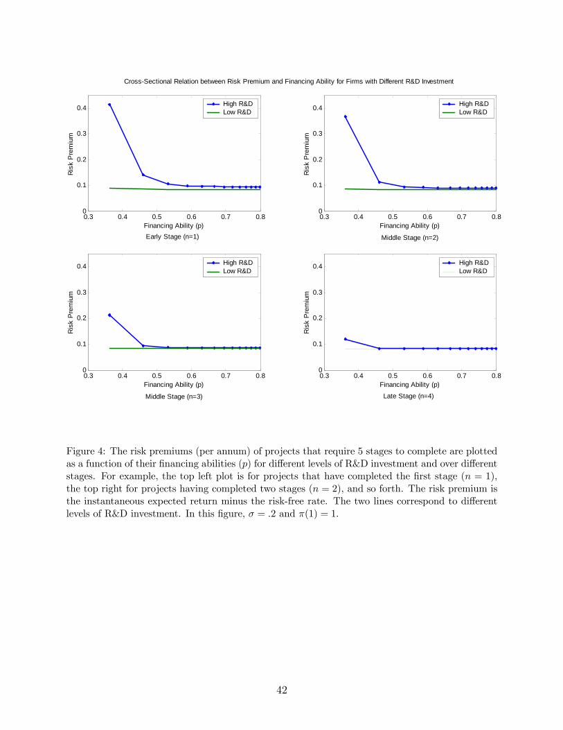
0.3 0.4 0.5 0.6 0.7 0.80

0.1

0.2

0.3

0.4

Financing Ability (p)

Ris

k P

rem

ium

High R&DLow R&D

0.3 0.4 0.5 0.6 0.7 0.80

0.1

0.2

0.3

0.4

Financing Ability (p)

Ris

k P

rem

ium

High R&DLow R&D

0.3 0.4 0.5 0.6 0.7 0.80

0.1

0.2

0.3

0.4

Financing Ability (p)

Ris

k P

rem

ium

High R&DLow R&D

0.3 0.4 0.5 0.6 0.7 0.80

0.1

0.2

0.3

0.4

Financing Ability (p)

Ris

k P

rem

ium

High R&DLow R&D

Early Stage (n=1) Middle Stage (n=2)

Middle Stage (n=3) Late Stage (n=4)

Cross-Sectional Relation between Risk Premium and Financing Ability for Firms with Different R&D Investment

Figure 4: The risk premiums (per annum) of projects that require 5 stages to complete are plottedas a function of their financing abilities (p) for different levels of R&D investment and over differentstages. For example, the top left plot is for projects that have completed the first stage (n = 1),the top right for projects having completed two stages (n = 2), and so forth. The risk premium isthe instantaneous expected return minus the risk-free rate. The two lines correspond to differentlevels of R&D investment. In this figure, σ = .2 and π(1) = 1.

42

5 10 15 20 250

0.1

0.2

0.3

0.4

0.5

R&D Investment (x)

Ris

k P

rem

ium

5 10 15 20 250

0.1

0.2

0.3

0.4

0.5

R&D Investment (x)

Ris

k P

rem

ium

5 10 15 20 250

0.1

0.2

0.3

0.4

0.5

R&D Investment (x)

Ris

k P

rem

ium

5 10 15 20 250

0.1

0.2

0.3

0.4

0.5

R&D Investment (x)

Ris

k P

rem

ium

Cross-sectional Relation between Risk Premium and R&D Investment for Firms with Different Financing Abilities

Early Stage (n=1) Middle Stage (n=2)

Middle Stage (n=3) Late Stage (n=4)

More Constrained More Constrained

More Constrained More Constrained

Less Constrained

Less Constrained

Less Constrained

Less Constrained

Figure 5: The risk premiums (per annum) of projects that require 5 stages to complete are plotted asa function of their investment requirement (x) for different financing abilities (p) and over differentstages. For example, the top left plot is for projects that have completed the first stage (n = 1),the top right for projects having completed two stages (n = 2), and so forth. The risk premium isthe instantaneous expected return minus the risk-free rate. The two lines correspond to differentexternal financing abilities (p). In this figure, σ = .2 and π(1) = 1.

43

0 0.1 0.2 0.3 0.40

0.1

0.2

0.3

0.4

0.5

R&D Intensity (x/V)

Ris

k P

rem

ium

0 0.1 0.2 0.3 0.40

0.1

0.2

0.3

0.4

0.5

R&D Intensity (x/V)

Ris

k P

rem

ium

0 0.1 0.2 0.3 0.40

0.1

0.2

0.3

0.4

0.5

R&D Intensity (x/V)

Ris

k P

rem

ium

0 0.1 0.2 0.3 0.40

0.1

0.2

0.3

0.4

0.5

R&D Intensity (x/V)

Ris

k P

rem

ium

Cross-sectional Relation between Risk Premium and R&D Intensity for Firms with Different Financing Abilities

Less Constrained

More Constrained More Constrained

More Constrained More Constrained

Less Constrained

Less Constrained Less Constrained

Early Stage (n=1) Middle Stage (n=2)

Middle Stage (n=3) Late Stage (n=4)

Figure 6: The risk premiums (per annum) of projects that require 5 stages to complete are plotted asa function of their investment intensity (x/V ) for different financing abilities (p) and over differentstages. For example, the top left plot is for projects that have completed the first stage (n = 1),the top right for projects having completed two stages (n = 2), and so forth. The risk premium isthe instantaneous expected return minus the risk-free rate. The two lines correspond to differentexternal financing abilities (p). In this figure, σ = .2 and π(1) = 1.

44

0.3 0.4 0.5 0.6 0.7 0.80.08

0.085

0.09

0.095

0.1

0.105

0.11

0.115

Financing Ability (p)

Ris

k P

rem

ium

High R&DLow R&D

0.3 0.4 0.5 0.6 0.7 0.80.08

0.085

0.09

0.095

0.1

0.105

0.11

0.115

Financing Ability (p)

Ris

k P

rem

ium

High R&DLow R&D

0.3 0.4 0.5 0.6 0.7 0.80.08

0.085

0.09

0.095

0.1

0.105

0.11

0.115

Financing Ability (p)

Ris

k P

rem

ium

High R&DLow R&D

0.3 0.4 0.5 0.6 0.7 0.80.08

0.085

0.09

0.095

0.1

0.105

0.11

0.115

Financing Ability (p)

Ris

k P

rem

ium

High R&DLow R&D

Early Stage (n=1) Middle Stage (n=2)

Middle Stage (n=3) Late Stage (n=4)

Cross-Sectional Relation between Risk Premium and Financing Ability for Firms with Different R&D Investment

Figure 7: The risk premiums (per annum) of projects that require 5 stages to complete are plottedas a function of their financing abilities (p) for different levels of R&D investment and over differentstages. For example, the top left plot is for projects that have completed the first stage (n = 1),the top right for projects having completed two stages (n = 2), and so forth. The risk premium isthe instantaneous expected return minus the risk-free rate. The two lines correspond to differentlevels of R&D investment. In this figure, σ = .4 and π(1) = 2.

45

5 10 15 20 250.08

0.1

0.12

0.14

0.16

0.18

0.2

0.22

R&D Investment (x)

Ris

k P

rem

ium

High Financing AbilityLow Financing Ability

5 10 15 20 250.08

0.1

0.12

0.14

0.16

0.18

0.2

0.22

R&D Investment (x)

Ris

k P

rem

ium

High Financing AbilityLow Financing Ability

5 10 15 20 250.08

0.1

0.12

0.14

0.16

0.18

0.2

0.22

R&D Investment (x)

Ris

k P

rem

ium

High Financing AbilityLow Financing Ability

5 10 15 20 250.08

0.1

0.12

0.14

0.16

0.18

R&D Investment (x)

Ris

k P

rem

ium

High Financing AbilityLow Financing Ability

Cross-sectional Relation between Risk Premium and R&D Investment for Firms with Different Financing Abilities

R&D Investment (x)Early Stage (n=1)

R&D Investment (x)

R&D Investment (x)

Middle Stage (n=2)

Middle Stage (n=3) Late Stage (n=4)

Figure 8: The risk premiums (per annum) of projects that require 5 stages to complete are plotted asa function of their investment requirement (x) for different financing abilities (p) and over differentstages. For example, the top left plot is for projects that have completed the first stage (n = 1),the top right for projects having completed two stages (n = 2), and so forth. The risk premium isthe instantaneous expected return minus the risk-free rate. The two lines correspond to differentexternal financing abilities (p). In this figure, σ = .4 and π(1) = 3.

46

0 0.1 0.2 0.3 0.4 0.50.08

0.1

0.12

0.14

0.16

0.18

0.2

0.22

R&D Intensity (x/V)

Ris

k P

rem

ium

High Financing AbilityLow Financing Ability

0.05 0.1 0.15 0.2 0.25 0.3 0.35 0.40.08

0.1

0.12

0.14

0.16

0.18

0.2

0.22

R&D Intensity (x/V)

Ris

k P

rem

ium

High Financing AbilityLow Financing Ability

0 0.05 0.1 0.15 0.2 0.25 0.3 0.350.08

0.1

0.12

0.14

0.16

0.18

0.2

0.22

R&D Intensity (x/V)

Ris

k P

rem

ium

High Financing AbilityLow Financing Ability

0 0.05 0.1 0.15 0.20.08

0.1

0.12

0.14

0.16

0.18

R&D Intensity (x/V)

Ris

k P

rem

ium

High Financing AbilityLow Financing Ability

Cross-sectional Relation between Risk Premium and R&D Intensity for Firms with Different Financing Abilities

Early Stage (n=1) Middle Stage (n=2)

Middle Stage (n=3) Late Stage (n=4)

Figure 9: The risk premiums (per annum) of projects that require 5 stages to complete are plotted asa function of their investment intensity (x/V ) for different financing abilities (p) and over differentstages. For example, the top left plot is for projects that have completed the first stage (n = 1),the top right for projects having completed two stages (n = 2), and so forth. The risk premium isthe instantaneous expected return minus the risk-free rate. The two lines correspond to differentexternal financing abilities (p). In this figure, σ = .4 and π(1) = 3.

47

Summary of R&D Firms

Number R&D Market Fiscal of Expenditure Capitalization Capital Book Book Total Year Firms ($Billions) ($Billions) Sales Earnings Expenditure Equity Equity Assets1975 1825 14.7 466.0 1.7% 35.5% 20.4% 4.1% 11.2% 5.2%1980 1654 28.6 796.7 1.7% 34.3% 20.0% 5.0% 12.4% 5.5%1985 2062 49.5 1027.9 2.9% 83.7% 38.1% 8.0% 20.8% 8.8%1990 2001 70.9 1450.5 3.3% 77.5% 44.6% 9.6% 25.6% 8.0%1995 2618 106.4 3201.2 3.9% 75.8% 54.0% 11.5% 29.6% 8.8%2000 2876 172.9 8511.5 4.8% 114.0% 69.8% 10.4% 26.0% 9.4%2005 2238 188.7 7066.8 4.1% 60.2% 83.6% 8.9% 25.4% 9.1%

Number R&D Market Industry of Expenditure Capitalization Capital Book Book Total

(SIC Code) Firms ($Billions) ($Billions) Sales Earnings Expenditure Equity Equity Assets

Drugs & 344 50.4 1156.7 18.2% 137.9% 301.5% 19.0% 51.2% 27.1%pharmaceuticals (283)

Computer programming, 365 25.6 926.4 10.3% 81.7% 265.7% 13.1% 39.3% 19.8%software, & services (737)

Electrical equipment 354 29.0 725.5 9.0% 103.9% 140.1% 13.5% 38.1% 22.2%excluding computers (36)

Measuring 323 12.0 378.8 6.6% 111.0% 176.9% 9.9% 28.6% 15.2%Instruments (38)

Computers & office 118 15.3 452.2 5.7% 86.4% 232.6% 12.1% 36.6% 18.0% equipment (357)

Total 1504 132.2 3639.6

Panel B: Selected Industries (Fiscal 2005)R&D Expenditure R&D Capital

relative to relative to

Panel A: All Firms doing R&DR&D Expenditure R&D Capital

relative to relative to

Table 1: For selected fiscal years from 1975 to 2005, Panel A reports the descriptive statistics forall firms with either positive R&D expenditure or positive R&D capital, which is computed as aweighted sum of the R&D expenditure over the past 5 years assuming a 20 percent amortization rate.All firms with Compustat data available are included except the utility and financial industries.Panel B reports the summary statistics of firms in selected high-tech industries for fiscal 2005.

48

High-tech Industry Distribution of R&D Capital / Total Assets Groups (June 2004; Percentage)

SIC Industry Low R&D Middle R&D High R&D

28 Drugs and pharmaceuticals 4.2 12.4 21.9

35 Computer equipment 5.1 12.6 9.2

36 Electrical equipment excluding computers 5.2 18.3 21.3

38 Measuring instruments; medical goods 3.8 16.7 12.0

73 Computer programming, software, & services 5.5 16.4 23.9

87 Research, development, and testing services 1.6 2.5 6.0

Total 25.4 78.8 94.3

Table 2: In June 2004, three R&D portfolios are formed based on the rank of the ratio of R&Dcapital to total assets. This table shows how the firms are distributed within the selected high-techindustries. All domestic firms trading on NYSE, AMEX, and NASDAQ with COMPUSTAT dataavailable are included.

49

Portfolio Characteristics, 1975-2004

Number of Age Market Book-to- Cash Debt / Cash / R&D/ R&D/ Volatility ofPortfolio Firms (Months) Cap (MM) Market Flow/PPE Total Capital PPE Cash CapExp R&D/CapExp1 (Low) 415 128 907 1.09 0.22 0.36 1.36 0.03 0.00 0.13

2 394 231 1795 0.89 0.21 0.33 1.98 1.39 0.21 0.313 398 205 2073 0.76 0.10 0.29 2.00 2.45 0.77 1.014 398 160 1310 0.74 -0.28 0.23 3.69 3.24 2.03 2.11

5 (High) 398 95 224 0.70 -5.56 0.15 11.73 4.34 16.55 13.94

Number of Age Market Book-to- Cash Debt / Cash / R&D/ R&D/ Volatility ofPortfolio Firms (Months) Cap (MM) Market Flow/PPE Total Capital PPE Cash TA R&D/TA1 (Low) 450 125 773 1.10 4.45 0.37 2.33 0.01 0.00 0.00

2 429 214 1620 0.95 -0.26 0.34 3.55 1.11 0.02 0.013 432 209 1418 0.82 -0.26 0.28 3.55 2.45 0.08 0.034 432 161 1887 0.71 -0.64 0.22 5.81 2.96 0.18 0.06

5 (High) 432 101 381 0.64 -5.10 0.16 7.50 4.48 0.59 0.22

Number of Age Market Book-to- Cash Debt / Cash / R&D/ R&D/ Volatility ofPortfolio Firms (Months) Cap (MM) Market Flow/PPE Total Capital PPE Cash ME R&D / ME1 (Low) 421 122 850 1.05 4.73 0.35 2.73 0.03 0.00 0.00

2 400 194 2647 0.61 0.00 0.25 5.16 1.21 0.01 0.013 404 184 1630 0.64 -0.54 0.26 4.07 2.23 0.03 0.024 404 181 829 0.76 -2.78 0.25 5.76 3.06 0.07 0.04

5 (High) 404 137 317 1.14 -2.50 0.24 4.06 4.91 0.25 0.12

Number of Age Market Book-to- Cash Debt / Cash / R&D/ Sales Dividend/Portfolio Firms (Months) Cap (MM) Market Flow/PPE Total Capital PPE Cash Growth PPE

1 (Least Constrained) 675 152 1303.60 0.70 2.97 0.07 15.60 1.00 1.11 1.002 676 200 1560.81 0.80 0.33 0.21 1.31 1.21 0.21 0.053 676 176 1051.29 0.99 0.23 0.27 0.54 2.24 0.18 0.024 676 149 566.36 1.17 0.10 0.38 0.28 3.04 0.36 0.01

5 (Most Constrained) 675 114 264.09 1.09 -4.98 0.64 1.44 5.05 0.85 0.00

Number of Age Market Book-to- Cash Debt / Cash / R&D/ Sales Dividend/Portfolio Firms (Months) Cap (MM) Market Flow/PPE Total Capital PPE Cash Growth PPE

1 (Least Constrained) 618 344 4764.79 0.81 0.79 0.37 1.83 1.33 0.22 0.132 598 193 478.78 0.91 0.44 0.33 1.65 1.18 0.17 0.093 619 130 169.06 0.97 0.41 0.31 2.59 1.95 0.29 0.084 598 113 72.21 1.02 -0.06 0.30 3.88 2.91 0.80 0.10

5 (Most Constrained) 619 100 23.45 0.89 -1.87 0.25 4.60 3.69 0.63 0.07

Panel C. Characteristics of Portfolios Classified by R&D Expenditure Relative to Market Value of Equity (R&D / ME)

Panel D. Characteristics of Portfolios Classified by KZ Index

Panel E. Characteristics of Portfolios Classified by WW Index

Panel A. Characteristics of Portfolios Classified by R&D Expenditure Relative to Capital Expenditure (R&D / CapExp)

Panel B. Characteristics of Portfolios Classified by R&D Capital Relative to Total Assets (R&D / TA)

Table 3: Summary statistics, from 1975 to 2004, for portfolios formed by ranking in each Juneof year t all NYSE-AMEX-NASDAQ firms excluding utility and financial firms. We compute thecross-sectional average of the characteristics for each year and then take a simple mean of the 30annual values.

50

Monthly Stock Returns and R&D Intensity

Number Monthly Portfolio Adjusted AdjustedPortfolio of Firms Excess Return Monthly Return alpha rm-rf smb hml R-square

Missing 2159 1.09% 0.16% -0.03% 1.04 0.93 0.23 89%3.33 1.47 -0.30 31.72 12.01 3.74

Low 638 0.88% 0.03% -0.10% 0.98 0.88 0.45 67%2.69 0.27 -0.49 16.45 6.79 3.90

Middle 645 1.01% 0.27% 0.21% 1.05 0.80 -0.12 87%2.95 3.33 1.75 23.05 10.89 -1.47

High 638 1.50% 0.73% 0.68% 1.02 1.42 -0.44 81%3.20 4.09 3.29 16.70 12.79 -4.26

Number Monthly Portfolio Adjusted AdjustedPortfolio of Firms Excess Return Monthly Return alpha rm-rf smb hml R-square

Missing 2017 1.06% 0.14% -0.06% 1.04 0.92 0.23 89%3.26 1.24 -0.52 32.00 12.00 3.74

Low 685 0.88% 0.02% -0.10% 0.97 0.91 0.44 67%2.65 0.14 -0.49 15.95 6.77 3.71

Middle 693 0.96% 0.22% 0.14% 1.02 0.81 -0.06 86%2.87 2.64 1.22 22.35 10.33 -0.73

High 688 1.59% 0.82% 0.76% 1.04 1.38 -0.43 81%3.42 4.62 3.82 17.07 12.01 -4.25

Number Monthly Portfolio Adjusted AdjustedPortfolio of Firms Excess Return Monthly Return alpha rm-rf smb hml R-square

Missing 2129 1.08% 0.15% -0.04% 1.04 0.92 0.23 89%3.30 1.36 -0.38 31.68 11.99 3.74

Low 649 0.71% -0.02% -0.20% 0.99 0.88 0.27 68%2.07 -0.16 -0.98 16.33 6.45 2.18

Middle 656 0.84% 0.20% 0.06% 1.04 0.83 -0.16 88%2.42 2.59 0.49 23.72 11.13 -2.12

High 646 1.87% 0.89% 0.96% 1.01 1.40 -0.20 79%4.25 5.04 4.78 16.26 12.72 -1.94

Panel C. Portfolios Based on R&D Expenditure / MVE

Panel A. Portfolios Based on R&D Expenditure / Capital Expenditure

Panel B. Portfolios Based on R&D Capital / Total Assets

Table 4: This table shows how stock returns vary with the R&D intensities. Each June of yeart from 1975 to 2004, we rank firms based on RD intensities into three equal-numbered portfoliosbased on the accounting data in fiscal year ending in calendar year t−1. We compute the subsequentmonthly returns from July of year t to June of year t+1 and reform the portfolios in June of yeart+ 1. The excess return is the difference between portfolio return and one-month T-bill rate. Theportfolio adjusted return is based on the difference between each individual stock’s return and thereturn of its matching portfolio by its size and book-to-market ranks. For each portfolio, the firstline reports the mean returns and regression coefficients from the Fama-French three-factor modelincluding the market factor (rm-rf), the size factor (smb), and the book-to-market factor (hml);the second line reports the heteroscedasticity robust t statistics. Portfolio returns are adjusted fordelisting bias.

51

Monthly Stock Returns and Financial Constraints Indices

Number Monthly Portfolio Adjusted AdjustedPortfolio of Firms Excess Return Monthly Return alpha rm-rf smb hml R-square

Missing 1101 1.04% 0.25% -0.04% 1.11 1.12 -0.12 85%2.59 1.62 -0.23 25.09 11.85 -1.48

Low 1009 1.03% 0.23% 0.23% 0.95 0.93 -0.08 87%3.09 2.92 1.84 26.55 15.09 -1.56

Middle 1006 1.10% 0.25% 0.21% 0.97 0.82 0.19 88%3.70 4.18 2.06 22.99 12.60 2.66

High 981 1.15% 0.32% 0.14% 1.02 0.97 0.28 79%3.39 2.73 0.93 20.36 9.70 3.04

Number Monthly Portfolio Adjusted AdjustedPortfolio of Firms Excess Return Monthly Return alpha rm-rf smb hml R-square

Missing 1257 1.17% 0.27% 0.10% 1.05 1.16 -0.09 86%2.97 1.78 0.67 26.60 14.55 -1.21

Low 994 0.72% 0.04% -0.19% 1.11 0.42 0.32 92%2.57 0.57 -2.09 40.62 6.67 6.22

Middle 947 0.85% 0.03% -0.04% 1.04 0.90 0.04 87%2.50 0.40 -0.37 22.56 10.88 0.45

High 929 1.37% 0.59% 0.48% 0.92 1.26 -0.05 75%3.43 4.30 2.43 16.05 12.28 -0.51

Panel A. Portfolios Based on KZ Index

Panel B. Portfolios Based on WW Index

Table 5: This table shows how stock returns vary with financial constraints indices. Each June ofyear t from 1975 to 2004, we rank firms based on the lagged financial constraint index into threeequal-numbered groups. We compute the subsequent returns from July of year t to June of yeart + 1 and reform the portfolios in June of year t + 1. The excess return is the difference betweenportfolio return and one-month T-bill rate. The portfolio adjusted return is based on the differencebetween each individual stock’s return and the return of its matching portfolio by its size andbook-to-market ranks. For each portfolio, the first line reports the mean returns and regressioncoefficients from the Fama-French three-factor model including the market factor (rm-rf), the sizefactor (smb), and the book-to-market factor (hml); the second line reports the heteroscedasticityrobust t statistics. Portfolio returns are adjusted for delisting bias.

52

Financial Constraints Factor Constructed from the WW Index

Number Equal-Weighted Value-Weightedof Monthly Monthly

Portfolio Label Firms Excess Return Excess Return

Small-cap Firms

Low WW 11 19 1.74% 1.31%

Middle WW 12 190 1.24% 1.14%

High WW 13 667 1.77% 0.97%

Mid-cap Firms

Low WW 21 169 0.86% 0.84%

Middle WW 22 538 0.83% 0.77%

High WW 23 270 0.58% 0.51%

Large-cap Firms

Low WW 31 810 0.69% 0.55%

Middle WW 32 243 0.59% 0.63%

High WW 33 23 0.12% 0.10%

Financial Constraints Factor (13+23+33)/3- -0.38% -0.55%(High WW - Low WW) (11+21+31)/3 (-1.18) (-1.56)

Table 6: This table shows how stock returns vary with the WW index within each size group. EachJune of year t, we form portfolios based on independent sorts of the top third, middle third, andbottom third of size (market capitalization in June of year t) and of lagged WW. We then computethe portfolio returns in excess of the one-month T-bill rate for the subsequent twelve months. Thebottom two rows report the mean excess returns and the t statistic for the financial constraintsfactor created from the WW index. All returns are adjusted for delisting bias following Shumwayand Warther (1999) and Shumway (1997). The sample period is from January 1975 to December2004.

53

Financial Constraints Factor Constructed from the KZ Index

Number Equal-Weighted Value-Weightedof Monthly Monthly

Portfolio Label Firms Excess Return Excess Return

Small-cap Firms

Low KZ 11 239 1.65% 1.15%

Middle KZ 12 294 1.70% 1.27%

High KZ 13 446 1.79% 0.98%

Mid-cap Firms

Low KZ 21 358 0.88% 0.80%

Middle KZ 22 333 1.05% 1.02%

High KZ 23 319 0.66% 0.60%

Large-cap Firms

Low KZ 31 424 0.71% 0.60%

Middle KZ 32 385 0.71% 0.54%

High KZ 33 223 0.64% 0.47%

Financial Constraints Factor (13+23+33)/3- -0.05% -0.16%(High KZ - Low KZ) (11+21+31)/3 (-0.39) (-1.45)

Table 7: This table shows how stock returns vary with the KZ index within each size group. EachJune of year t, we form portfolios based on independent sorts of the top third, middle third, andbottom third of size (market capitalization in June of year t) and of KZ using accounting variablesreported in the fiscal year ending in calendar year t − 1. We then compute the portfolio returnsin excess of the one-month T-bill rate for the subsequent twelve months. The bottom two rowsreport the mean excess returns and the t statistic for the financial constraints factor created fromthe KZ index. All returns are adjusted for delisting bias following Shumway and Warther (1999)and Shumway (1997). The sample period is from January 1975 to December 2004.

54

Financial Constraints (KZ) and Stock Returns within R&D Capital / Total Assets Groups

MatchingNumber Monthly Portfolio

of Excess Adjusted AdjustedPortfolio Label Firms Return Return alpha m s h R-Square

Low R&D Capital / Total Assets

Low KZ 11 208 0.82% -0.01% -0.06% 0.98 0.70 0.26 86%2.86 -0.05 -0.57 27.01 8.57 4.00

Middle KZ 12 201 1.05% 0.15% 0.04% 0.99 0.86 0.55 64%3.24 1.12 0.19 16.20 6.56 4.79

High KZ 13 202 0.84% -0.01% -0.21% 1.02 0.90 0.48 74%2.57 -0.06 -1.24 21.89 8.09 5.00

High - Low 13 -11 0.02% 0.00% -0.15% 0.04 0.21 0.22 6%0.14 -0.03 -1.00 1.25 3.43 3.10

Middle R&D Capital / Total Assets

Low KZ 21 207 0.83% 0.10% 0.05% 0.99 0.83 -0.14 86%2.39 0.87 0.36 26.06 13.02 -2.11

Middle KZ 22 201 1.02% 0.22% 0.20% 0.99 0.63 0.12 85%3.50 2.99 1.80 24.31 10.01 1.75

High KZ 23 197 1.23% 0.42% 0.27% 1.01 0.97 0.19 78%3.55 3.69 1.77 16.50 9.32 1.67

High - Low 23 - 21 0.41% 0.34% 0.13% 0.07 0.23 0.45 17%2.65 2.66 0.91 1.76 3.07 6.52

High R&D Capital / Total Assets

Low KZ 31 222 1.20% 0.56% 0.42% 1.04 1.23 -0.50 83%2.61 3.42 2.17 15.85 10.92 -5.21

Middle KZ 32 219 1.58% 0.80% 0.83% 1.01 1.29 -0.40 80%3.50 5.12 3.82 17.49 12.84 -4.73

High KZ 33 216 1.80% 1.19% 0.75% 1.17 1.60 -0.26 75%3.36 5.13 2.96 15.80 9.81 -1.84

High - Low 33 - 31 0.60% 0.63% 0.32% 0.13 0.37 0.24 12%3.24 4.00 1.94 3.01 3.69 2.49

Table 8: This table shows the relation between postranking stock returns and financial constraintsmeasured by the KZ index for different R&D intensity groups. The portfolios are formed in eachJune on a conditional two-way sorts on the lagged R&D intensity first and then on the lagged KZindex. Monthly portfolio returns are then computed over the next 12 months. The excess returnis the difference between the raw portfolio return and the one-month T-bill rate. The matchingportfolio adjusted return is based on the difference between the individual stock return and thereturn of its matching portfolio by size and book-to-market ranks. The alphas are estimated asintercepts from the regressions of excess portfolio postranking returns on the Fama-French factorreturns. m is the coefficient of the market factor; s is the coefficient of the size factor; h is thecoefficient of the book-to-market factor. For each portfolio, the first line reports the mean returnsand the regression estimates, and the second line reports heteroscedasticity-robust t statistics.All portfolio returns are adjusted for delisting bias. The sample period is from January 1975 toDecember 2004.

55

Financial Constraints (KZ) and Stock Returns within R&D Capital / Total Assets Groups

AdjustedPortfolio Label alpha m s h u l R-square

Low R&D Capital / Total Assets

Low KZ 11 0.15% 0.94 0.71 0.18 -0.13 -0.09 88%1.23 28.25 10.99 2.95 -2.66 -2.02

Middle KZ 12 0.30% 0.92 0.86 0.43 -0.13 -0.16 67%1.45 16.34 7.59 4.40 -2.13 -2.47

High KZ 13 0.01% 0.95 0.89 0.36 -0.05 -0.19 76%0.05 22.69 9.72 4.09 -0.79 -2.48

High - Low 13 -11 -0.14% 0.01 0.19 0.18 0.08 -0.10 7%-0.94 0.41 3.24 2.59 1.83 -1.98

Middle R&D Capital / Total Assets

Low KZ 21 0.36% 0.97 0.88 -0.20 -0.33 0.01 91%2.86 31.05 15.81 -3.20 -7.07 0.30

Middle KZ 22 0.40% 0.95 0.64 0.06 -0.15 -0.07 87%3.78 23.38 11.57 0.84 -4.41 -2.06

High KZ 23 0.56% 0.95 0.98 0.07 -0.16 -0.16 81%3.54 15.78 10.95 0.66 -2.97 -2.71

High - Low 23 - 21 0.12% 0.02 0.18 0.38 0.19 -0.20 25%0.84 0.49 2.78 5.89 4.37 -3.76

High R&D Capital / Total Assets

Low KZ 31 0.71% 1.04 1.30 -0.52 -0.38 0.09 86%3.85 20.43 11.07 -6.53 -5.26 1.18

Middle KZ 32 1.03% 1.00 1.32 -0.44 -0.22 0.01 81%4.60 17.88 12.12 -5.12 -3.47 0.10

High KZ 33 1.10% 1.11 1.63 -0.38 -0.27 -0.10 77%3.91 16.23 9.83 -3.11 -2.50 -0.86

High - Low 33 - 31 0.38% 0.07 0.33 0.15 0.12 -0.19 16%2.11 1.60 3.70 1.85 1.67 -2.48

Table 9: This table shows the relation between postranking stock returns and financial constraintsmeasured by the KZ index for different R&D intensity groups. The portfolios are formed in eachJune on a conditional two-way sorts on the lagged R&D intensity first and then on the laggedKZ index. Monthly portfolio returns are then computed over the next 12 months. The alphasare estimated as intercepts from the regressions of excess portfolio postranking returns on theFama-French factor returns, the momentum factor returns, and the liquidity factor returns. mis the loading on the market factor; s is the loading on the size factor; h is the loading on thebook-to-market factor; u is the loading on the momentum factor; l is the loading on the liquidityfactor. For each portfolio, the first line reports the regression estimates, and the second line reportsheteroscedasticity-robust t statistics. The sample period is from January 1975 to December 2004.All portfolio returns are adjusted for delisting bias.

56

Financial Constraints (KZ) and Stock Returns within R&D/MVE Groups

MatchingNumber Monthly Portfolio

of Excess Adjusted AdjustedPortfolio Label Firms Return Return alpha m s h R-Square

Low R&D Expenditure / MVE

Low KZ 11 195 0.68% 0.01% -0.12% 1.01 0.65 0.04 88%2.24 0.13 -1.08 31.98 9.44 0.74

Middle KZ 12 189 0.91% 0.10% -0.04% 0.99 0.82 0.41 65%2.77 0.74 -0.18 16.22 6.14 3.47

High KZ 13 190 0.77% 0.03% -0.27% 1.02 0.92 0.43 71%2.26 0.18 -1.52 21.25 6.94 3.85

High - Low 13 -11 0.09% 0.02% -0.15% 0.01 0.27 0.39 12%0.48 0.10 -0.91 0.37 2.83 4.07

Middle R&D Expenditure / MVE

Low KZ 21 199 0.73% 0.11% 0.01% 1.00 0.89 -0.33 87%1.96 0.99 0.09 24.71 13.64 -5.03

Middle KZ 22 192 0.99% 0.29% 0.21% 1.01 0.64 -0.03 87%3.19 4.09 1.91 24.96 9.34 -0.40

High KZ 23 190 0.88% 0.22% -0.05% 1.06 0.97 0.06 82%2.44 2.02 -0.36 18.76 10.06 0.54

High - Low 23 - 21 0.14% 0.11% -0.17% 0.11 0.17 0.51 19%0.88 0.89 -1.16 2.65 2.04 6.50

High R&D Expenditure / MVE

Low KZ 31 206 1.57% 0.71% 0.70% 1.03 1.37 -0.35 79%3.35 3.69 3.20 14.78 10.70 -3.15

Middle KZ 32 202 1.74% 0.76% 0.86% 1.00 1.34 -0.09 77%4.06 4.91 3.93 17.03 12.86 -1.11

High KZ 33 200 2.11% 1.27% 1.00% 1.12 1.51 0.02 75%4.39 6.26 4.28 16.33 11.77 0.16

High - Low 33 - 31 0.54% 0.56% 0.30% 0.09 0.14 0.36 8%3.25 3.84 1.85 2.15 1.78 5.03

Table 10: This table shows the relation between postranking stock returns and financial constraintsmeasured by the KZ index for different R&D intensity groups. The R&D intensity is measured bythe ratio of R&D expenditure to year-end market value of equity. The portfolios are formed in eachJune on a conditional two-way sorts on the lagged R&D intensity first and then on the lagged KZindex. Monthly portfolio returns are then computed over the next 12 months. The excess returnis the difference between the raw portfolio return and the one-month T-bill rate. The matchingportfolio adjusted return is based on the difference between the individual stock return and thereturn of its matching portfolio by size and book-to-market ranks. The alphas are estimated asintercepts from the regressions of excess portfolio postranking returns on the Fama-French factorreturns. m is the coefficient of the market factor; s is the coefficient of the size factor; h is thecoefficient of the book-to-market factor. For each portfolio, the first line reports the mean returnsand the regression estimates, and the second line reports heteroscedasticity-robust t statistics.All portfolio returns are adjusted for delisting bias. The sample period is from January 1975 toDecember 2004.

57

Financial Constraints (KZ) and Stock Returns within R&D Expenditure / Capital Expenditure Groups

MatchingNumber Monthly Portfolio

of Excess Adjusted AdjustedPortfolio Label Firms Return Return alpha m s h R-Square

Low R&D Expenditure / Capital Expenditure

Low KZ 11 197 0.87% 0.05% -0.02% 0.98 0.65 0.30 87%3.14 0.48 -0.17 30.29 9.04 4.91

Middle KZ 12 190 1.01% 0.12% 0.01% 1.00 0.82 0.53 65%3.14 0.96 0.04 16.38 6.21 4.65

High KZ 13 191 0.82% -0.01% -0.23% 1.03 0.90 0.47 75%2.50 -0.08 -1.41 23.29 8.70 5.22

High - Low 13 -11 -0.05% -0.07% -0.22% 0.05 0.25 0.17 7%-0.33 -0.51 -1.47 1.53 4.65 2.55

Middle R&D Expenditure / Capital Expenditure

Low KZ 21 200 0.81% 0.08% 0.05% 1.02 0.77 -0.18 87%2.34 0.80 0.38 26.83 11.60 -2.69

Middle KZ 22 193 1.10% 0.34% 0.30% 1.02 0.66 0.01 86%3.54 4.61 2.67 24.43 11.11 0.09

High KZ 23 190 1.26% 0.49% 0.33% 1.07 0.99 0.03 81%3.42 4.36 2.16 17.79 10.57 0.29

High - Low 23 - 21 0.47% 0.42% 0.18% 0.10 0.32 0.33 16%3.18 3.57 1.30 2.66 4.73 5.19

High R&D Expenditure / Capital Expenditure

Low KZ 31 195 1.14% 0.51% 0.34% 1.03 1.29 -0.47 82%2.47 3.11 1.74 15.73 11.72 -4.97

Middle KZ 32 191 1.52% 0.73% 0.76% 0.99 1.37 -0.42 78%3.25 4.22 3.32 16.16 12.99 -4.48

High KZ 33 189 1.76% 1.11% 0.72% 1.11 1.59 -0.20 74%3.40 5.07 2.79 15.05 10.82 -1.47

High - Low 33 - 31 0.62% 0.60% 0.37% 0.09 0.30 0.27 9%3.52 4.00 2.18 1.93 3.70 3.27

Table 11: This table shows the relation between postranking stock returns and financial constraintsmeasured by the KZ index for different R&D intensity groups. The portfolios are formed in eachJune on a conditional two-way sorts on the lagged R&D intensity first and then on the lagged KZindex. Monthly portfolio returns are then computed over the next 12 months. The excess returnis the difference between the raw portfolio return and the one-month T-bill rate. The matchingportfolio adjusted return is based on the difference between the individual stock return and thereturn of its matching portfolio by size and book-to-market ranks. The alphas are estimated asintercepts from the regressions of excess portfolio postranking returns on the Fama-French factorreturns. m is the coefficient of the market factor; s is the coefficient of the size factor; h is thecoefficient of the book-to-market factor. For each portfolio, the first line reports the mean returnsand the regression estimates, and the second line reports heteroscedasticity-robust t statistics.All portfolio returns are adjusted for delisting bias. The sample period is from January 1975 toDecember 2004.

58

Financial Constraints (WW) and Stock Returns within R&D Expenditure / MVE Groups

MatchingNumber Monthly Portfolio

of Excess Adjusted AdjustedPortfolio Label Firms Return Return alpha m s h R-Square

Low R&D Expenditure / MVE

Low WW 11 189 0.61% 0.01% -0.22% 1.09 0.31 0.23 87%2.19 0.15 -1.93 32.48 3.98 3.94

Middle WW 12 187 0.52% -0.20% -0.43% 1.08 0.84 0.16 84%1.52 -1.54 -2.97 25.40 8.25 2.01

High WW 13 182 0.79% 0.09% -0.17% 0.96 1.05 0.21 70%2.15 0.55 -0.82 18.99 10.04 2.14

High - Low 13 -11 0.18% 0.08% 0.05% -0.13 0.74 -0.02 27%0.74 0.54 0.22 -2.61 10.02 -0.19

Middle R&D Expenditure / MVE

Low WW 21 196 0.62% 0.01% -0.18% 1.09 0.28 0.20 88%2.23 0.13 -1.71 35.31 4.83 3.57

Middle WW 22 187 0.78% 0.13% 0.02% 1.06 0.90 -0.30 87%2.07 1.42 0.17 23.57 12.63 -4.37

High WW 23 192 0.91% 0.34% 0.00% 1.02 1.34 -0.22 80%2.04 2.37 -0.01 18.61 12.64 -2.06

High - Low 23 - 21 0.28% 0.33% 0.18% -0.07 1.05 -0.41 50%0.94 2.27 0.84 -1.13 10.64 -3.68

High R&D Expenditure / MVE

Low WW 31 189 1.13% 0.36% 0.13% 1.19 0.89 0.08 83%2.95 2.60 0.80 23.07 13.07 1.10

Middle WW 32 188 1.70% 0.78% 0.74% 1.07 1.45 -0.26 81%3.58 4.25 3.43 17.06 12.65 -2.45

High WW 33 183 2.31% 1.46% 1.33% 0.97 1.77 -0.27 69%4.24 5.52 4.28 10.92 9.70 -1.73

High - Low 33 - 31 1.17% 1.10% 1.19% -0.23 0.87 -0.35 27%3.59 4.68 4.07 -2.75 5.65 -2.52

Table 12: This table shows the relation between postranking stock returns and financial constraintsmeasured by the WW index for different R&D intensity groups. The R&D intensity is measured bythe ratio of R&D expenditure to year-end market value of equity. The portfolios are formed in eachJune on a conditional two-way sorts on the lagged R&D intensity first and then on the lagged WWindex. Monthly portfolio returns are then computed over the next 12 months. The excess returnis the difference between the raw portfolio return and the one-month T-bill rate. The matchingportfolio adjusted return is based on the difference between the individual stock return and thereturn of its matching portfolio by size and book-to-market ranks. The alphas are estimated asintercepts from the regressions of excess portfolio postranking returns on the Fama-French factorreturns. m is the coefficient of the market factor; s is the coefficient of the size factor; h is thecoefficient of the book-to-market factor. For each portfolio, the first line reports the mean returnsand the regression estimates; and the second line reports heteroscedasticity-robust t statistics.All portfolio returns are adjusted for delisting bias. The sample period is from January 1975 toDecember 2004.

59

R&D Intensity and Stock Returns within Financial Constraints (KZ) Groups

MatchingNumber Monthly Portfolio

of Excess Adjusted AdjustedPortfolio Label Firms Return Return alpha m s h R-Square

Low KZ

Low R&D Capital / Total Assets 11 235 0.80% 0.00% -0.05% 0.99 0.67 0.18 88%2.74 -0.02 -0.50 29.14 9.18 2.98

Middle R&D Capital / Total Assets 12 230 1.02% 0.27% 0.27% 0.96 1.09 -0.19 74%2.59 2.14 1.30 15.51 9.41 -1.65

High R&D Capital / Total Assets 13 227 1.33% 0.66% 0.66% 0.99 1.24 -0.64 79%2.84 3.75 3.00 14.55 9.32 -5.76

High - Low 13 -11 0.54% 0.69% 0.63% 0.03 0.64 -0.75 50%1.91 3.07 2.86 0.41 4.13 -6.57

Middle KZ

Low R&D Capital / Total Assets 21 216 0.96% 0.09% -0.04% 1.02 0.75 0.44 83%3.26 0.82 -0.29 28.07 8.72 6.43

Middle R&D Capital / Total Assets 22 211 0.98% 0.16% 0.12% 1.00 0.65 0.20 86%3.41 2.12 1.13 20.50 9.55 2.32

High R&D Capital / Total Assets 23 213 1.61% 0.82% 0.80% 1.05 1.25 -0.29 78%3.62 5.26 3.69 17.56 11.25 -3.35

High - Low 23 - 21 0.60% 0.74% 0.71% 0.07 0.48 -0.73 49%2.33 3.43 3.61 1.21 3.57 -7.57

High KZ

Low R&D Capital / Total Assets 31 179 0.81% -0.05% -0.23% 1.00 0.86 0.50 71%2.49 -0.31 -1.31 20.54 7.70 5.23

Middle R&D Capital / Total Assets 32 181 1.25% 0.46% 0.15% 1.08 1.01 0.42 77%3.51 3.30 0.88 23.53 8.97 4.50

High R&D Capital / Total Assets 33 179 1.80% 1.19% 0.72% 1.16 1.62 -0.21 73%3.34 5.06 2.82 15.31 9.88 -1.39

High - Low 33 - 31 0.99% 1.24% 0.96% 0.16 0.76 -0.71 47%3.00 4.71 4.08 2.26 5.26 -5.71

Table 13: This table shows the relation between postranking stock returns and R&D intensity fordifferent level of KZ groups. The portfolios are formed in each June on a conditional two-way sortson the lagged KZ index first and then on the lagged R&D intensity. Monthly portfolio returnsare then computed over the next 12 months. The excess return is the difference between the rawportfolio return and the one-month T-bill rate. The matching portfolio adjusted return is based onthe difference between the individual stock return and the return of its matching portfolio by sizeand book-to-market ranks. The alphas are estimated as intercepts from the regressions of excessportfolio postranking returns on the Fama-French factor returns. m is the coefficient of the marketfactor; s is the coefficient of the size factor; h is the coefficient of the book-to-market factor. Foreach portfolio, the first line reports the mean returns and the regression estimates, and the secondline reports heteroscedasticity-robust t statistics. All portfolio returns are adjusted for delistingbias. The sample period is from January 1975 to December 2004.

60

R&D Intensity and Stock Returns within Financial Constraints (KZ) Groups

AdjustedPortfolio Label alpha m s h u l R-square

Low KZ

Low R&D Capital / Total Assets 11 0.21% 0.94 0.69 0.09 -0.19 -0.09 91%2.08 30.27 13.31 1.74 -4.95 -2.39

Middle R&D Capital / Total Assets 12 0.50% 0.95 1.14 -0.22 -0.31 0.06 77%2.47 17.68 10.15 -2.13 -5.96 1.05

High R&D Capital / Total Assets 13 0.90% 1.02 1.32 -0.62 -0.40 0.15 82%4.04 18.42 9.51 -6.37 -4.55 1.60

High - Low 13 -11 0.63% 0.09 0.68 -0.66 -0.20 0.21 53%2.96 1.49 4.59 -7.22 -2.66 2.11

Middle KZ

Low R&D Capital / Total Assets 21 0.20% 0.96 0.76 0.34 -0.14 -0.12 86%1.43 27.85 10.86 4.93 -2.26 -2.50

Middle R&D Capital / Total Assets 22 0.31% 0.95 0.66 0.12 -0.10 -0.11 88%2.96 20.04 11.26 1.44 -3.08 -3.44

High R&D Capital / Total Assets 23 1.04% 1.02 1.28 -0.35 -0.21 -0.03 80%4.80 18.10 10.56 -4.48 -3.90 -0.46

High - Low 23 - 21 0.69% 0.10 0.49 -0.69 -0.07 0.09 49%3.75 2.10 3.69 -8.59 -1.38 1.08

High KZ

Low R&D Capital / Total Assets 31 -0.02% 0.92 0.84 0.37 -0.03 -0.21 73%-0.11 21.01 9.23 4.21 -0.39 -2.84

Middle R&D Capital / Total Assets 32 0.49% 0.99 1.01 0.26 -0.14 -0.23 81%2.90 22.07 12.35 3.52 -2.14 -3.03

High R&D Capital / Total Assets 33 1.10% 1.09 1.65 -0.34 -0.27 -0.13 75%3.72 15.09 10.46 -2.71 -2.28 -1.09

High - Low 33 - 31 1.12% 0.16 0.81 -0.71 -0.24 0.08 49%4.37 2.71 5.39 -6.78 -2.66 0.82

Table 14: This table shows the relation between postranking stock returns and R&D intensity fordifferent level of KZ groups. The portfolios are formed in each June on a conditional two-way sortson the lagged KZ index first and then on the lagged R&D intensity. The alphas are estimated asintercepts from the regressions of excess portfolio postranking returns on the Fama-French factorreturns, the momentum factor returns, and the liquidity factor returns. m is the loading on themarket factor; s is the loading on the size factor; h is the loading on the book-to-market factor; uis the loading on the momentum factor; l is the loading on the liquidity factor. For each portfolio,the first line reports the regression estimates; and the second line reports heteroscedasticity-robustt statistics. All portfolio returns are adjusted for delisting bias. The sample period is from January1975 to December 2004.

61

R&D Intensity and Stock Returns within Financial Constraints (KZ) Groups

MatchingNumber Monthly Portfolio

of Excess Adjusted AdjustedPortfolio Label Firms Return Return alpha m s h R-Square

Low KZ

Low R&D Expenditure / MVE 11 224 0.67% 0.03% -0.10% 1.00 0.65 -0.03 89%2.17 0.29 -0.89 34.12 10.31 -0.56

Middle R&D Expenditure / MVE 12 219 0.86% 0.16% 0.12% 0.96 1.04 -0.22 75%2.18 1.36 0.59 15.77 9.03 -1.88

High R&D Expenditure / MVE 13 215 1.62% 0.76% 0.86% 0.97 1.32 -0.45 77%3.55 4.00 3.87 13.87 9.58 -3.79

High - Low 13 -11 0.96% 0.75% 0.87% 0.01 0.74 -0.32 37%3.76 3.31 4.03 0.08 5.02 -2.83

Middle KZ

Low R&D Expenditure / MVE 21 204 0.84% 0.07% -0.12% 1.04 0.69 0.36 84%2.84 0.60 -0.95 29.00 8.17 5.39

Middle R&D Expenditure / MVE 22 200 0.92% 0.21% 0.09% 1.04 0.66 0.04 87%2.96 2.67 0.87 21.24 8.49 0.50

High R&D Expenditure / MVE 23 200 1.76% 0.78% 0.88% 1.00 1.31 -0.08 76%4.16 5.09 4.05 16.84 12.04 -0.94

High - Low 23 - 21 0.87% 0.72% 0.88% -0.01 0.59 -0.45 38%3.65 3.31 4.34 -0.16 4.33 -4.50

High KZ

Low R&D Expenditure / MVE 31 166 0.83% 0.04% -0.24% 1.01 0.92 0.51 68%2.43 0.24 -1.28 19.50 6.50 4.35

Middle R&D Expenditure / MVE 32 167 0.94% 0.33% -0.13% 1.13 1.12 0.18 80%2.38 2.41 -0.77 25.17 10.50 1.88

High R&D Expenditure / MVE 33 165 2.13% 1.28% 1.03% 1.12 1.50 0.00 73%4.36 5.97 4.15 15.52 11.57 0.01

High - Low 33 - 31 1.30% 1.24% 1.27% 0.11 0.58 -0.51 35%4.62 4.98 5.51 1.70 4.58 -4.94

Table 15: This table shows the relation between postranking stock returns and R&D intensity fordifferent level of KZ groups. The R&D intensity is measured as the ratio of R&D expenditure toyear-end market value of equity. The portfolios are formed in each June on a conditional two-waysorts on the lagged KZ index first and then on the lagged R&D intensity. Monthly portfolio returnsare then computed over the next 12 months. The excess return is the difference between the rawportfolio return and the one-month T-bill rate. The matching portfolio adjusted return is based onthe difference between the individual stock return and the return of its matching portfolio by sizeand book-to-market ranks. The alphas are estimated as intercepts from the regressions of excessportfolio postranking returns on the Fama-French factor returns. m is the coefficient of the marketfactor; s is the coefficient of the size factor; h is the coefficient of the book-to-market factor. Foreach portfolio, the first line reports the mean returns and the regression estimates, and the secondline reports heteroscedasticity-robust t statistics. All portfolio returns are adjusted for delistingbias. The sample period is from January 1975 to December 2004.

62

R&D Intensity and Stock Returns within Financial Constraints (KZ) Groups

MatchingNumber Monthly Portfolio

of Excess Adjusted AdjustedPortfolio Label Firms Return Return alpha m s h R-Square

Low KZ

Low R&D Expenditure / Capital Expenditure 11 221 0.82% 0.03% -0.02% 0.99 0.66 0.18 89%2.87 0.32 -0.24 34.88 11.66 3.23

Middle R&D Expenditure / Capital Expenditure 12 215 1.06% 0.31% 0.32% 1.00 1.06 -0.27 74%2.60 2.43 1.51 15.39 8.76 -2.23

High R&D Expenditure / Capital Expenditure 13 213 1.26% 0.58% 0.57% 0.97 1.30 -0.60 79%2.70 3.30 2.63 14.44 10.43 -5.49

High - Low 13 -11 0.44% 0.57% 0.50% 0.01 0.71 -0.70 51%1.56 2.63 2.41 0.10 5.61 -6.69

Middle KZ

Low R&D Expenditure / Capital Expenditure 21 201 0.94% 0.10% -0.05% 1.03 0.70 0.45 84%3.27 0.91 -0.41 28.58 8.32 6.81

Middle R&D Expenditure / Capital Expenditure 22 197 0.97% 0.18% 0.12% 1.02 0.67 0.12 87%3.21 2.41 1.16 21.29 10.09 1.38

High R&D Expenditure / Capital Expenditure 23 198 1.62% 0.79% 0.80% 1.02 1.29 -0.25 78%3.66 5.14 3.62 17.00 12.13 -2.92

High - Low 23 - 21 0.62% 0.70% 0.72% 0.03 0.56 -0.71 51%2.43 3.39 3.70 0.51 4.56 -7.52

High KZ

Low R&D Expenditure / Capital Expenditure 31 162 0.86% 0.01% -0.19% 1.01 0.86 0.50 71%2.64 0.06 -1.03 20.86 7.52 5.21

Middle R&D Expenditure / Capital Expenditure 32 164 1.20% 0.43% 0.10% 1.14 1.02 0.34 80%3.25 3.26 0.57 24.46 9.55 3.94

High R&D Expenditure / Capital Expenditure 33 162 1.75% 1.13% 0.70% 1.11 1.60 -0.18 72%3.34 4.94 2.67 14.66 10.73 -1.31

High - Low 33 - 31 0.89% 1.12% 0.88% 0.10 0.74 -0.69 44%2.75 4.33 3.65 1.47 5.36 -5.70

Table 16: This table shows the relation between postranking stock returns and R&D intensity fordifferent level of KZ groups. The portfolios are formed in each June on a conditional two-way sortson the lagged KZ index first and then on the lagged R&D intensity. Monthly portfolio returnsare then computed over the next 12 months. The excess return is the difference between the rawportfolio return and the one-month T-bill rate. The matching portfolio adjusted return is based onthe difference between the individual stock return and the return of its matching portfolio by sizeand book-to-market ranks. The alphas are estimated as intercepts from the regressions of excessportfolio postranking returns on the Fama-French factor returns. m is the coefficient of the marketfactor; s is the coefficient of the size factor; h is the coefficient of the book-to-market factor. Foreach portfolio, the first line reports the mean returns and the regression estimates, and the secondline reports heteroscedasticity-robust t statistics. All portfolio returns are adjusted for delistingbias. The sample period is from January 1975 to December 2004.

63

R&D Intensity and Stock Returns within Financial Constraints (WW) Groups

MatchingNumber Monthly Portfolio

of Excess Adjusted AdjustedPortfolio Label Firms Return Return alpha m s h R-Square

Low WW

Low R&D Expenditure / MVE 11 183 0.62% -0.02% -0.23% 1.07 0.36 0.26 86%2.21 -0.16 -1.97 32.50 4.81 4.38

Middle R&D Expenditure / MVE 12 185 0.58% -0.01% -0.21% 1.09 0.28 0.16 89%2.07 -0.16 -1.97 34.97 4.69 2.96

High R&D Expenditure / MVE 13 183 1.01% 0.28% 0.04% 1.19 0.56 0.25 86%3.09 2.90 0.31 31.93 9.00 3.95

High - Low 13 -11 0.39% 0.30% 0.27% 0.12 0.20 -0.01 12%2.78 2.18 1.91 3.13 3.72 -0.15

Middle WW

Low R&D Expenditure / MVE 21 182 0.52% -0.23% -0.44% 1.08 0.83 0.21 83%1.55 -1.76 -3.08 24.97 7.95 2.62

Middle R&D Expenditure / MVE 22 178 0.76% 0.09% -0.01% 1.08 0.96 -0.34 88%1.95 0.99 -0.07 23.47 12.73 -4.78

High R&D Expenditure / MVE 23 183 1.38% 0.51% 0.35% 1.16 1.34 -0.11 84%3.07 3.05 1.93 20.91 15.93 -1.28

High - Low 23 - 21 0.86% 0.74% 0.79% 0.08 0.51 -0.32 35%3.96 3.36 4.19 1.38 4.48 -3.55

High WW

Low R&D Expenditure / MVE 31 199 0.83% 0.15% -0.10% 0.95 1.09 0.12 71%2.19 0.91 -0.49 18.45 10.12 1.15

Middle R&D Expenditure / MVE 32 203 1.15% 0.54% 0.22% 1.03 1.41 -0.24 79%2.48 3.55 1.06 16.57 12.51 -2.24

High R&D Expenditure / MVE 33 199 2.35% 1.47% 1.35% 0.98 1.78 -0.24 72%4.38 5.56 4.58 11.49 10.26 -1.68

High - Low 33 - 31 1.53% 1.32% 1.45% 0.03 0.70 -0.36 34%5.71 4.56 6.28 0.39 3.87 -2.91

Table 17: This table shows the relation between postranking stock returns and R&D intensity fordifferent level of WW groups. The R&D intensity is measured as the ratio of R&D expenditure toyear-end market value of equity. The portfolios are formed in each June on a conditional two-waysorts on the lagged WW index first and then on the lagged R&D intensity. Monthly portfolioreturns are then computed over the next 12 months. The excess return is the difference betweenthe raw portfolio return and the one-month T-bill rate. The matching portfolio adjusted return isbased on the difference between the individual stock return and the return of its matching portfolioby size and book-to-market ranks. The alphas are estimated as intercepts from the regressionsof excess portfolio postranking returns on the Fama-French factor returns. m is the coefficient ofthe market factor; s is the coefficient of the size factor; h is the coefficient of the book-to-marketfactor. For each portfolio, the first line reports the mean returns and the regression estimates, andthe second line reports heteroscedasticity-robust t statistics. All portfolio returns are adjusted fordelisting bias. The sample period is from January 1975 to December 2004.

64