financial dollarization: the role of banks and interest rates · pdf filefinancial...

ISSN 1561081-0

9 7 7 1 5 6 1 0 8 1 0 0 5

WORKING PAPER SER IESNO 748 / MAY 2007

FINANCIALDOLLARIZATION

THE ROLE OF BANKSAND INTEREST RATES

by Henrique S. Basso,Oscar Calvo-Gonzalezand Marius Jurgilas

In 2007 all ECB publications

feature a motif taken from the €20 banknote.

WORK ING PAPER SER IE SNO 748 / MAY 2007

This paper can be downloaded without charge from http://www.ecb.int or from the Social Science Research Network

electronic library at http://ssrn.com/abstract_id=983483.

FINANCIALDOLLARIZATION

THE ROLE OF BANKSAND INTEREST RATES 1

by Henrique S. Basso 2,Oscar Calvo-Gonzalez 3

and Marius Jurgilas 4

1 We thank an anonymous referee of the ECB Working Paper Series for many useful comments. Any views expressed in this paper are those of the authors and do not necessarily represent those of the ECB.

2 School of Economics, Mathematics and Statistics, Birkbeck College, University of London, Malet Street, London, WC1E 7HX, United Kingdom; e-mail: [email protected]

3 European Central Bank, Kaiserstrasse 29, 60311 Frankfurt am Main, Germany;

4 Department of Economics, College of Liberal Arts, University of Connecticut,341 Mansfield Road, Unit1063, CT 06269-1063 USA;

e-mail: [email protected]

e-mail: [email protected]

© European Central Bank, 2007

AddressKaiserstrasse 2960311 Frankfurt am Main, Germany

Postal addressPostfach 16 03 1960066 Frankfurt am Main, Germany

Telephone +49 69 1344 0

Internethttp://www.ecb.int

Fax +49 69 1344 6000

Telex411 144 ecb d

All rights reserved.

Any reproduction, publication and reprint in the form of a different publication, whether printed or produced electronically, in whole or in part, is permitted only with the explicit written authorisation of the ECB or the author(s).

The views expressed in this paper do not necessarily reflect those of the European Central Bank.

The statement of purpose for the ECB Working Paper Series is available from the ECB website, http://www.ecb.int.

ISSN 1561-0810 (print)ISSN 1725-2806 (online)

3ECB

Working Paper Series No 748 May 2007

CONTENTS

Abstract 4

Non-technical summary 5

1 Introduction 7

2 Model 10

2.1 Households 11

2.2 Deposits and loans aggregator 14

2.3 Banks 15

2.4 Equilibrium 17

2.5 Extensions 18

2.5.1 Endogenous foreign funds 18

2.5.2 Model with firms 19

3 Model solution and main implications 23

3.1 Model extensions results 27

3.1.1 Endogenous foreign funds – results 27

3.1.2 Model with firms – results 29

4 Data and methodology 30

4.1 Data 4.2 Descriptive statistics 35

4.3 Methodology 42

5 Estimation results 43

6 Conclusions 52

Appendix A 54

Appendix B 56

References 71

European Central Bank Working Paper Series 73

30

AbstractThis paper develops a model to explain the determinants of finan-

cial dollarization. Expanding on the existing literature, our frameworkallows interest rate differentials to play a role in explaining financialdollarization. It also accounts for the increasing presence of foreignbanks in the local financial sector. Using a newly compiled data seton transition economies we find that increasing access to foreign fundsleads to higher credit dollarization, while it decreases deposit dollar-ization. Interest rate differentials matter for the dollarization of bothloans and deposits. Overall, the empirical results lend support to thepredictions of our theoretical model.

JEL classification: E44, G21Keywords: Financial Dollarization; Foreign Banks; Interest Rate Dif-ferentials; Transition Economies

4ECB Working Paper Series No 748 May 2007

Non-technical summary

Why do households and firms in many countries borrow in foreign currencies?Why do they hold deposits in foreign currencies? This paper addresses thesequestions theoretically and empirically using a newly compiled data set ontransition economies, a region which has not been traditionally the focus ofthe so-called “financial dollarization” literature. This lack of attention by theliterature is all the more surprising given that financial dollarization is indeedprevalent, and in some cases growing, among the formerly planned economies.Financial dollarization increases the exposure of agents to exchange rate riskand can therefore become a potential source of macroeconomic and financialinstability. Hence, understanding the determinants of financial dollarizationis of great interest not only to researchers but also to policy-makers. Dataavailability and the lack of an overall theoretical framework have hithertobeen the main constraints to improving our understanding of financial dol-larization. In this paper we contribute to the literature both theoreticallyand empirically.

On the theory of financial dollarization, we expand on the existing lit-erature by modeling explicitly how competition among banks, and the factthat banks often have an open facility to increase funds by accumulating for-eign liabilities, may affect local currency and foreign currency interest ratedifferentials. The feature that banks can accumulate foreign liabilities ismotivated by the widespread experience in the transition countries, wheremany banks are now subsidiaries of foreign banks and have ample access toforeign sources of funding from their parent banks. Introducing imperfectcompetition in the banking market and letting banks borrow abroad to funddomestic credit growth allows us to incorporate a departure from uncoveredinterest rate parity. We are therefore able to address the common argumentthat interest rate differentials between loans in foreign and local currency area key factor behind credit dollarization. This is an argument which cannotbe addressed within theoretical frameworks such as the so-called minimumvariance portfolio approach, which assumes that the uncovered interest rateparity holds and explains financial dollarization as a portfolio choice prob-lem in which agents choose the currency composition of their portfolio thatminimizes the variance of returns (local currency assets have uncertain re-turns due to domestic inflation and foreign currency assets have uncertaindue to real exchange rate risk). Recognizing the important insights from theminimum variance portfolio approach our modeling strategy is to nest the

minimum variance portfolio approach and expand on it.

5ECB


Our second contribution to the literature is empirical. We compile a newdata set on financial dollarization in transition economies and use it to testthe main predictions of our model. Our data set shows that dollarizationof deposits is not generally matched by the dollarization of credit - a resultwhich is difficult to square with some of the existing theories of financialdollarization but is consistent with our framework. In particular, it fits withthe argument that foreign borrowing by banks is being used to fund domesticcredit growth. As banks have to keep net open positions under a limit, theygo on to lend in foreign currency to domestic borrowers and we observe arise in credit dollarization without deposit dollarization being necessarilyaffected. Our data set is also particularly rich in terms of the availability ofdata split on credit and deposit dollarization split for households and firms.The main predictions of the model are confirmed in our empirical analysis asfollows:

First, access to foreign funds increases credit dollarization but it decreasesthe dollarization of deposits. The underlying intuition is the access of banksto foreign borrowing, often from their parent banks, as already mentioned.This implies that the accumulation of foreign liabilities seen in transitioncountries results in currency mismatches in the agents’ portfolios in thesecountries.

Second, interest rate differentials matter. As expected in our model, awider interest rate differential on loans in domestic currency compared toloans in foreign currency increases loan dollarization. A wider interest ratedifferential on deposits (again local currency interest rate minus foreign cur-rency interest rate) has a negative effect on the extent of deposit dollarization.

Third, in line with the literature on the minimum variance portfolio ap-proach, the trade off between inflation and real exchange rate variability isfound to be a significant factor explaining financial dollarization.

Fourth, a higher degree of openness of an economy contributes to loandollarization - but it appears to do so only in the case of firms and not house-holds. In general the explanatory power of our model is lower for householddollarization, calling for more research efforts particularly in that area.

Overall, our analysis provides both a theoretical motivation as well asempirical validation that the access of banks to foreign funds and interestrate differentials between local and foreign currency instruments affect theextent of financial dollarization in transition economies.


1 Introduction

Why do households and firms in many countries borrow in foreign curren-cies? Why do they hold deposits in foreign currencies? This paper addressesthese questions theoretically and empirically using a newly compiled dataset on transition economies, a region which has not been traditionally thefocus of the so-called “financial dollarization” (FD) literature. As noted ina recent survey, this lack of attention by the literature is all the more sur-prising given that FD is indeed prevalent, and in some cases growing, amongthe formerly planned economies (Levy-Yeyati (2006)). Moreover, high ex-change rate exposure has been recently highlighted as a potential source ofmacroeconomic and financial instability in a number of central and south-east European economies (Winkler and Beck (2006), Standard and Poor’s -RatingsDirect (2006)).

Until recently, the literature on FD (defined as the holding by residents ofa share of their assets and/or liabilities denominated in foreign currency) haslacked both an overall encompassing framework as well as a broad empiricalbasis. Lack of data has led to the literature often focusing on either depositor credit dollarization but typically not both (e.g. Nicolo, Honohan, and Ize(2005)). Having a broader view is important because theoretical explanationscan often help to explain the dollarization of deposits but not credit, or theother way around. If, for example, agents perceived the currency to beovervalued, assumption that the literature usually does, then the safe heavenportfolio approach can only explain why households hold deposits in foreigncurrency but not why they are borrowing in foreign currency.

In a recent survey of the literature, Ize and Levy-Yeyati (2005) dividethe main contributions to the theoretical analysis of FD into three mainparadigms: (a) the price risk-portfolio choice; (b) credit risk; and, (c) fi-nancial environment. The portfolio choice approach, as its name suggests,explains FD as the result of a portfolio choice by which agents minimizethe variance of the portfolio returns. Returns of local currency assets areuncertain due to domestic inflation while returns of foreign currency assetsare uncertain due to real exchange rate risk. This approach focuses on vari-ances since any interest rate differentials are assumed to be cancelled out byexpected exchange rate movements, thus the uncovered interest rate parity(UIP) holds. The credit risk paradigm explains FD as the result of optimaldecisions by risk neutral agents in the presence of default risk (enhancedby moral hazard/asymmetric information) while the financial environment

7ECB


paradigm explains FD as the result of domestic market and legal imperfec-tions.

It is, however, difficult to find unequivocal empirical support for any ofthe above paradigms as the three explanations overlap to some extent (a sig-nificant variable in explaining FD could be linked to two or even all theories).This calls for a unified analytical framework. Ize (2005) provides one suchapproach based on an investor/household sector that decides on its depositsbased on the minimum variance portfolio choice paradigm, while risk neutralfirms choose the currency composition of their borrowing in the presence ofdefault risk. The results are obtained based on the assumption that theremight exist an overvaluation overhang due to the fact that governments donot adjust the exchange rate within a specific interval.

Two key aspects of Ize (2005) should be highlighted. Firstly, contraryto most other contributions, which look at FD only from the depositorsside,1 Ize’s model explains both deposit and credit dollarization. Depositors(households) choose foreign currency denominated assets motivated by the“safe heaven” portfolio (dollar denominated assets are one sided bets) whileborrowers (firms) choose foreign currency denominated loans to maximizetheir objective function in the presence of default risk. Secondly, despitethis separation of the motives of investors and firms, the model requiresthe equilibrium to be defined as a point where depositors and borrowerschoose the same currency composition. This implies that banks are mereintermediaries without any influence in the final outcome and interest ratesare fully determined by the interaction between investors and firms.

However, the assumption that credit and deposit dollarization are alwaysmatched is not broadly supported by our data. In transition economies, onwhich we focus our empirical analysis, the shares of foreign currency loansand foreign currency deposits are often negatively correlated (see Table 5below). Credit dollarization has increased in these economies as banks inthe region, often foreign-owned, have been able to borrow abroad to fund asubstantial growth of domestic credit which - to keep the banks’ exposuresmatched - is granted in foreign currencies (see also Arcalean and Calvo-Gonzalez (2006)). Subsidiaries of foreign owned banks are often seen asdriving the fast credit growth in their attempt to capture market shares

1A relevant exception is Barajas and Morales (2003) who analysed, empirically, Dollar-ization of Liabilities (DL) in Latin America finding that Central Bank Foreign ExchangeMarket interventions and interest rate differential (interpreted as representing borrowersmarket power) are also important factors driving DL.


in yet undeveloped credit markets that are not only highly profitable butare also expected to grow substantially in the medium term.2 Therefore, inexplaining FD it is important to model explicitly two key features: (i) thedifferent extent to which dollarization affects credit and deposits; (ii) the rolethat competition among banks is playing in driving foreign currency lendingin these countries.

The latter has been addressed empirically in transition economies onlyby Luca and Petrova (2003), who concluded that banks, in attempting tomatch currency composition of their assets and liabilities, drive FD in theseeconomies. To our knowledge only Catao and Terrones (2000) provide atheoretical model of FD focused on the banking side. However, the loansand deposits decisions are not explicitly modeled, ad hoc loan demand func-tions are assumed while deposits are in infinite supply given a deposit rate.Moreover, foreign and local currency loans are not considered as substitutes.In their model FD is determined not only by the interest rate set by thebanks but mostly by the assumption that investors have different collateralcapabilities. Therefore, despite its novelty, the model does not allow one toisolate the impact of market and legal imperfections and banking activity onFD. Finally, their framework does not provide simple testable implications,limiting its use in empirical work.

As in Ize (2005) we model depositors and borrowers separately. In ourbasic framework, we do so by assuming that households have different dis-count factors, one being a borrower and one a lender. This contrasts to Ize’sapproach in which he assumes that firms are borrowers and households arelenders. However, in one extension to our model we also include firms thatborrow funds to finance investment opportunities.

Our main contribution to the literature is to model explicitly how compe-tition among banks, and the fact that banks have an open facility to increasefunds by accumulating foreign liabilities, may affect local currency and for-eign currency interest rate differentials. Crucially, we introduce imperfectcompetition in the banking market and allow foreign liabilities to be used in

2For evidence of the importance of targets for future market shares for foreign-ownedbanks active in the region such as ING and Raiffeisen see de Haas and Naaborg (2005).Recently, the high price at which a 62 percent stake in the Romanian bank BCR was sold(EUR 3.75 billion - the largest amount ever paid for a central and eastern European bank)was interpreted by market commentators as driven by the fact that BCR represented thelast big state-owned bank in the region giving at once a large market share for the buyer(The Banker (2006)).

9ECB


the loan market. This also allows us to incorporate a departure from uncov-ered interest rate parity. We would therefore be able to address the commonargument that interest rate differentials between loans in foreign and localcurrency are a key factor behind credit dollarization - an argument whichby construction cannot be addressed within the minimum variance portfolioapproach alone.

The main predictions of the model, which are indeed confirmed in our em-pirical results, are as follows. First, access to foreign funds increases creditdollarization but it decreases dollarization of deposits. Hence the increasingforeign presence in the banking sector coupled with accumulation of bank-ing foreign liabilities experienced in transition economies results in currencymismatches in the agents’ portfolios in these countries. Second, interest ratedifferentials matters. A wider interest rate differencial on loans positivelyaffects loan dollarization. Interest rate differential on deposits has a negativeeffect on deposit dollarization. Third, our results confirm the relevance of theminimum variance portfolio theory of dollarization. Fourth, higher degree ofopenness leads to higher corporate loan dollarization.

The remainder of the paper is organized as follows. Section 2 presents amodel of the currency choice while section 3 provides solutions and model im-plications. An overview of the data and methodology is presented in section4, section 5 presents the estimation results and section 6 concludes. Auxil-iary regression results and an alternative model specification are presentedin the appendix.

2 Model

Assume the economy is populated by an infinite number of banks i ∈ [0, 1],two representative households and a deposits and loans Dixit-Stiglitz CES“aggregator”. We assume that all economic agents live for two periods. Asan extension to our basic framework (see section 2.5) we also include firmsin the model.


2.1 Households

Each representative household has a specific discount factor, household H hasβH and household L has βL < βH . Both households have identical endow-ments in both periods (Y )3, hence the relationship between the interest ratecharged by banks and their implicit interest rate (1/βj) determines whetherthe household j = H,L decides to take a loan or make a deposit.

In equilibrium (formally stated below) the economies’ gross interest rateswill be between 1/βH and 1/βL. Note that due to imperfect competition inthe banking market there will be two rates, one for deposits and another forloans, for each currency. We will assume a set of parameter values for whichall four equilibrium rates will be inside that interval. Hence the householdwith low discount factor will find it better to borrow and consume more todayand the other will find it better to save and consume more tomorrow. Thatway a household that makes deposits (loans) does not take loans (deposits).

Households maximize utility given a stream of income choosing the amountof deposits and loans in local and foreign currency (implicitly determiningconsumption in each period). Both local and foreign currency denominatedassets are risky. While the first might fluctuate due to inflation, the secondwill fluctuate due to changes in the real exchange rate.

In order to incorporate competition among banks having only two rep-resentative households we assume that households (indirectly through the“aggregator”) choose CES deposits and loans indexes, which are a compositeof all banks deposits and loans given a constant elasticity of substitution4.That way the banking sector will be characterized by monopolistic compe-tition. Although we do not model why banks exist and where they derivetheir market power from, banks may be providing liquidity and hence reduc-ing the cost of credit (Freixas, Parigi, and Rochet 2000). The assumptionthat banks have market power is supported by empirical evidence (Simonsand Stavins 1998).

Each household is split into two units: (i) the investor, responsible fordeciding demand for loans and deposits5 or the set (D, L), where D = totaldeposits, L = total loans and (ii) the fund manager, responsible for deciding

3Endowments, as consumption, total deposits and loans, are in real terms. This doesnot affect the results of the model. Households may actually have unlimited access to anexchange rate spot market in each period.

4We assume the same elasticity of substitution for loans and deposits. Allowing fordifferent elasticity of substitution would not change the results of the model.

5Throughout the paper we state that households demand loans and deposits, consid-

11ECB


the portfolio compositions (αd, αl), where αd = portion of deposits in foreigncurrency (deposit dollarization) and αl = portion of loans in foreign currency(loan dollarization). This specification integrates the Minimum VariancePortfolio framework developed by Ize and Levy-Yeyati (2003). An alternativespecification where households make their decisions at once, rather than firstabout the demand for loans and deposits and then about their currencycomposition, is presented in Appendix A. As it is shown there the results arevery similar.

The investor part of the household solves a certainty equivalent problemgiven the expected returns, defined as E[R̄d] = (1−αd)Rd+αdR

∗d for deposits

and E[R̄l] = (1−αl)Rl +αlR∗l for loans. Note that the certainty equivalence

assumption allows us to solve this problem independently of the portfoliocomposition decision. Hence the variance of returns does not affect the totaldeposit or loan decisions6. The investor’s j = H,L problem is

max{D,L}

(Y −D + L)1−1/σ

1− 1/σ+ βj

(Y + E[R̄d]D − E[R̄l]L)1−1/σ

1− 1/σ

The fund manager allocates the deposits (D) and loans (L) determined bythe investor into foreign currency denominated deposits and loans (d∗, l∗) andlocal currency denominated deposits and loans (d, l) to maximize expectedreturn and minimize the variance of the resulting portfolio, where

D = d + d∗, d = (1− αd)D and d∗ = αdD

L = l + l∗, l = (1− αl)L and l∗ = αlL

Hence for deposits

maxαd

E[R̄d]− qV AR[R̄d]

2(1)

where

R̄d = (1− αd)R̂d + αdR̂∗d

R̂d = Rd − µπ

R̂∗d = R∗

d + µS

ering that both are products that banks sell to households. However, deposit “demand”is upward sloping as it represents a supply of funds.

6In the alternative specification shown in Appendix A these two decisions are madetogether and therefore the total demand decisions are affected negatively by the variance.


and µπ and µS are the risk component due to inflation and real exchangerate respectively by which the rate indexes need to be adjusted to get theactual returns (R̂d,R̂∗

d) in period 2. These have zero mean, variances givenby Sπ,π, SS,S and covariance by Sπ,S. Finally, q indicates the weight of thevariance term in the fund manager’s objective function.

The portfolio choice is therefore given by

αd =R∗

d −Rd

q(Sπ,π + SS,S + 2Sπ,S)+

Sπ,π + Sπ,S

(Sπ,π + SS,S + 2Sπ,S)

=R∗

d −Rd

q(Sπ,π + SS,S + 2Sπ,S)+ λMV P (2)

where, as in Ize and Levy-Yeyati (2003), λMV P affects dollarization posi-tively and is defined as

λMV P =Sπ,π + Sπ,S


The loans decision problem is similar to (1), though now fund managersminimize the payment and the variance.

maxαl

−E[R̄l]− qV AR[R̄l]

2(3)

where

R̄l = (1− αl)R̂l + αlR̂∗l

R̂l = Rl − µπ

R̂∗l = R∗

l + µS

The loans portfolio choice is given by

αl =Rl −R∗

l

q(Sπ,π + SS,S + 2Sπ,S)+

Sπ,π + Sπ,S


=Rl −R∗

l

q(Sπ,π + SS,S + 2Sπ,S)+ λMV P (4)

The equations determining the portfolio choice are the same as in Ize andLevy-Yeyati (2003). However, in their case αd = αl = λMV P as they assumeUIP holds. In our case banks choose interest rates such that households findit optimal to increase αl if loan differential (Rl−R∗

l ) increases and to decreaseαd if deposit differential (Rd −R∗

d) increases.

13ECB


2.2 Deposits and Loans Aggregator

The aggregator sells deposit and loan indexes to households and buys indi-vidual banks’ deposits and loans from each bank in order to minimize thecost for loans7 and maximize the gains for deposits8. We assume perfectcompetition so the aggregator makes no profits. The introduction of a de-posits and loans aggregator facilitates the exposition of the model withoutchanging its results. The aggregator solves the following problems.

Local Currency Deposits

min{di}

[∫ 1

0

1

rdi

di di

]

subject to total deposits in local currency, which is a CES index of all depositsin each bank i ∈ [0, 1]

d =

[∫ 1

0

(di)θ−1

θ di

] θθ−1

That implies the following demand for local currency deposits from bank i(di):

di =

[Rd

rdi

]−θ

d (5)

where rdi is the deposit rate given by bank i and the local currency depositrate index Rd is defined as

1

Rd

=

[∫ 1

0

(1

rdi

)1−θ

di

] 11−θ

.

Note that profits are indeed zero since∫ 1

01

rdidi di = 1

Rdd.

Local Currency Loans

min{li}

[∫ 1

0

rlilidi

]

7The household promises to pay an interest rate for the loans (l), thus the aggregatorwants to pay as little as possible for the individual loans made in each bank i.

8The aggregator promises to pay a deposit rate to the household, thus he/she will wantto maximize the deposit rate on each individual deposit or minimize the present value ofeach deposit.


subject to total loans in local currency which is a CES index of all loans donein each bank i ∈ [0, 1]

l =

[∫ 1

0

(li)θ−1

θ di

] θθ−1

That implies the following demand for local currency loans from bank i (li):

li =

[rliRl

]−θ

l (6)

where rli is the loan rate set by bank i and the local currency loan rate indexRl is defined as

Rl =

[∫ 1

0

(rli)1−θ di

] 11−θ

.

Note that, again, profits are zero since∫ 1

0rlilidi = Rll.

Similarly for foreign currency loans and deposits:

d∗i =

[R∗

d

rd∗i

]−θ

d∗ (7)

where1

R∗d

=

[∫ 1

0

(1

rd∗i

)1−θ

di

] 11−θ

l∗i =

[rl∗iR∗

l

]−θ

l∗ (8)

where R∗l =

[∫ 1

0

(rl∗i )1−θdi

] 11−θ

where rd∗i and rl∗i are bank i’s foreign currency deposit and loan rates andd∗i and l∗i are the demand for bank i’s foreign currency deposits and loans.R∗

d and R∗l are the respective interest rate indexes.

2.3 Banks

Each bank i chooses deposit and loan interest rates for foreign and localcurrency (rd∗i , rl

∗i , rdi, rli) to maximize its expected second period profits and

its loan market shares.

15ECB


Banks start with an amount of funds (F ), comprised of the banks’ capitaland its foreign liabilities, of which some are denominated in foreign currencyand some in local currency. Banks can use F to offset loans, hence we donot force the market of loans and deposits to match but allow banks to usethese funds to close the gap. The parameter φ indicates the portion of fundsthat are denominated in foreign currency.

As foreign banks have greater facility to acquire funds in foreign currencyfrom their parent banks, greater foreign bank penetration can be expectedto result in a higher share of funds denominated in foreign currency. There-fore foreign bank penetration is implicitly modelled here as φ. This link issupported by our data (see section 4).

Banks are assumed to have balanced currency positions thus loans mustbe equal to funds plus deposits for each currency.9 Given prudential regu-lations limiting net open foreign exchange positions this assumption is notunreasonable.

Bank i solves the following problem10:

max{rli,rl∗i ,rdi,rd∗i }

E

[(rli − 1) li + (rl∗i − 1)l∗i − (rdi − 1) di

− (rd∗i − 1)d∗i + γ

(lil

+l∗il∗

) ](9)

subject to demand functions (5)-(8) and

li = di + (1− φ)F (10)

l∗i = d∗i + φF (11)

where γ reflects how much the bank cares about loan shares. We includeloan market shares in the banks’ objective function for two main reasons.Firstly, as shown by de Haas and Naaborg (2005), foreign banks do set tar-gets for future market share for their subsidiaries in transition economies.Secondly, given that we solve a two period model, loan market shares will

9If banks are not assumed to hold balanced currency positions but some limit is imposedon currency exposures, the main qualitative results of the model remain unchanged as longas this limit eventually binds given the sizes of F and φ.

10The second period realization of individual bank rates have the same risk componentsdefined in the household problem, µπ and µS (e.g. rli = E[rli] − µπ). As banks are riskneutral and these have zero mean, they do not affect bank i’s problem.


also serve as a proxy for future profits. Alternatively one could solve an in-finite period model, assuming banks maximize the future stream of profits.However, that would increase the complexity of the problem and since thebanking sector is growing considerably in these economies there is a premiumfor first entrants that is not necessarily present in infinite period profit func-tions. In any case, the main qualitative results of our model do not changewhen loan market shares are dropped from the banks’ objective function.

The first order condition of the bank problem, incorporating the equilib-rium conditions (individual bank rates are equal to rate indexes, explainedbelow) are: (10), (11) and

γθ − Lαl(Rd(1 + θ) + Rl(1− θ)) = 0

γθ − L(1− αl)(R∗d(1 + θ) + R∗

l (1− θ)) = 0

2.4 Equilibrium

The equilibrium is defined as a set of individual banks’ interest rates{rdi, rd

∗i , rli, rl

∗i }1

i=0, interest rate indexes {Rd, R∗d, Rl, R

∗l } and loan and de-

posit demands {d, d∗, l, l∗} such that given interest rates, aggregate demandsolves the households’ problem, given aggregate demand and interest rateindexes, the set {rdi, rd

∗i , rli, rl

∗i } maximises bank i objective function for all

i ∈ [0, 1] and the following conditions hold11.

1

Rd

=

[∫ 1

0

(1

rdi

)1−θ

di

] 11−θ

Rl =

[∫ 1

0

(rli)1−θ di

] 11−θ

1

R∗d

=

[∫ 1

0

(1

rd∗i

)1−θ

di

] 11−θ

R∗l =

[∫ 1

0

(rl∗i )1−θ di

] 11−θ

11One can easily show that ensuring these, together with the individual bank demandequations used as constraints to bank i’s problem guarantees that the equations ford, d∗, l, l∗ used in the aggregator problem hold.

17ECB


As all banks are equal these conditions in fact imply that bank rates andrate indexes are equal.

2.5 Extensions

2.5.1 Endogenous Foreign Funds

An extension to our basic model is to allow banks to choose the requiredamount of foreign denominated funds given a pre-determined interest rate.This is important since it allows us to verify if exogeneity of funds is drivingthe results.

In addition this model extension is relevant because most foreign bankshave that facility open from their parent banks. Profits in transition economieshave generally been greater than in mature markets making this flow of fundsa profitable strategy for the parent bank.

Hence bank i now starts with an amount of funds in local currency FLC

but can choose funds in foreign currency FFC given an interest rate (EIB)12.The problem is

max{rli,rl∗i ,rdi,rd∗i ,FFC}

E


− (rd∗i − 1)d∗i − (EIB − 1)FFC + γ

(lil

+l∗il∗

) ]

subject to demand equations (5)-(8) and

li = di + FLC

l∗i = d∗i + FFC

As we will show in the next section, allowing for endogeneity of foreignfunds does not alter our main results.

12We implicitly assume that all external funds are denominated in foreign currency,following the “original sin” literature.


2.5.2 Model with Firms

The basic model in this paper included only risk averse households who seekto maximize the return and minimizing the variance of the loan/depositportfolio. However, corporate loan dollarization is also of interest. In fact,as our data set shows, it is sizeable and generally higher than household loandollarization. Therefore, we now extend the model to include firms which,as is common in the literature, we will assume to be risk neutral.

We assume that a representative firm has a project (investment oppor-tunity) available, whereby investing V at period 1 the firm will get MV atperiod 2, where M is the real return on the project and is stochastic. Wefurther assume that the firm has no funds in period 1 and hence is forcedto borrow the entire initial investment from banks. The firm maximizes ex-pected profits (Q) selecting the currency composition of the total amountborrowed from banks given the interest rates on each loan type. Profits arerisky due to variations in M , inflation (µπ) and real exchange rate (µS). Weassume these three stochastic processes are jointly normally distributed withmean [M̄, 0, 0]′ and variance Σ, where

Σ =

SM,M SM,π SM,S

Sπ,M Sπ,π Sπ,S

SS,M SS,π SS,S

.

In order to make the portfolio currency selection non-trivial we assumethat the firm may default if profits at period 2 are negative 13.

Formally, the firm problem is

max{αv}

E[Q] = max{αv}

E[max

{MV − R̄vV, 0

}]

where R̄v = (1− αv)R̂v + αvR̂∗v

R̂v = Rv − µπ

R̂∗v = R∗

v + µS

V = v + v∗

v = (1− αv)V

v∗ = αvV

13Under no default firms would select the currency for which the loan interest rate isthe lowest so the result would be total dollarization, no dollarization or indeterminacy (ifrates are equal).

19ECB


Following the same modelling simplification as in the basic model we alsointroduce a corporate loan aggregator or a syndicated loan manager. Thesyndicated loan manager receives loan demands v and v∗ from the firm andgets funding from each bank i to minimize the total loan costs (

∫ 1

0rvividi

and∫ 1

0rv∗i v

∗i di), such that v =

[∫ 1

0v

θ−1θ

i di] θ

θ−1

and v∗ =[∫ 1

0(v∗i )

θ−1θ di

] θθ−1

.

That way

vi =

[rvi

Rv

]−θ

v (12)

v∗i =

[rv∗iR∗

v

]−θ

v∗ (13)

where Rv =

[∫ 1

0

(rvi)1−θ di

] 11−θ

and R∗v =

[∫ 1

0

(rv∗i )1−θ di

] 11−θ

.

If the firm defaults the loan manager pays a cost of verification K andgets M(v +v∗) from the firm’s project. In order to simplify bank i’s problemwe assume that in case of a default the loan manager will charge Ki and K∗

i

such that each bank will get back Mvi−Ki = vi and Mv∗i −K∗i = v∗i or zero

net returns. This insurance mechanism is provided by a government agencythat effectively does a transfer for the loan manager to cover the gain or lossgiven the realizations of M such that the net profit of the loan aggregator iszero. The insurance mechanism, or the transfer, is provided as long as theloan manager’s expected return without the transfer is not smaller than thereturn he/she would get using the funds to make loans to the households(assumed to be risk free), hence

E[min{R̄vV, MV } − DefK] > V R̄l. (14)

Where Def is a dummy variable that takes the value 1 in case of defaultand zero otherwise. Note that this constraint will actually bind in equilibriumand is effectively a participation constraint for the loan manager to performthe loan.

Given the participation constraint, the firm problem can be modified asfollows (see Jeanne (2003) for more details)

max{αv}

E[Q] = max{αv}

[E

[max

{MV − R̄vV, 0

}]+ E[min{R̄vV, MV } − DefK]− V R̄l

]

max{αv}

E[Q] = max{αv}

[E[MV ]− E[Def]K − V R̄l

]


That implies that in order to maximize profits (Q) the firm actually seeksto minimize E[Def] or the probability of default. In the model presented byJeanne (2003) that would imply minimizing the variance since there, UIPholds. In our case, as expected interest rate from local and foreign currencyloans might not be the same, the problem of the firm becomes

min{αv}

Prob[Default] =

∫ 0

−∞Prob[Q]dQ

where Q = (M − (1− αv)R̂v − αvR̂∗v)V

= (M + (1− αv)µπ − αvµS − [(1− αv)Rv + αvR∗v])V.

Given our assumption of joint normality of M , µπ and µS, this problem, aftersome manipulation, becomes

min{αv}

Φ

((1− αv)Rv + αvR

∗v − M̄

σp

, 0, 1

)

Where Φ is the standard normal cumulative density function and σP2 =

SM,M + (1−αv)2Sπ,π + α2

vSS,S − 2(1−αv)αvSπ,S − 2αvSM,S + 2(1−αv)SM,π.The first order condition of this minimization is

R∗v −Rv

(Sπ,π + SS,S + 2Sπ,S)=

[(1− αv)Rv + αvR

∗v − M̄

σp

] (αv − λMV P − λCOV

)

(15)

Where λCOV =SM,π+SM,S

(Sπ,π+SS,S+2Sπ,S).

First note that if Rv = R∗v then the firm will only minimize the variance

(minαv σp2), hence αv = λMV P + λCOV . That way firm loan dollarization is

determined by the original trade-off between inflation and the real exchangerate (summarized by λMV P ) plus an additional term reflecting the optimalhedging strategy of firms as regards to the real return on their investments.

On the one hand, if the real return is positively correlated with the realexchange rate then choosing foreign currency denominated loans protectsthe firm against default; higher interest payment will occur when investmentreturns are high. Hence high SM,S leads to more dollarization.

On the other hand, if inflation and real investment returns are negativelycorrelated, then when inflation is low and interest rate payments are highthe investment return will also be high, protecting the firm against default.Thus, lower SM,π leads to less dollarization.

21ECB


If R∗v > Rv (assuming M̄ − (1 − αv)Rv − αv > 0 or the expected return

on investment is positive) then αv < λMV P +λCOV ; corporate loan dollariza-tion decreases. The firm shifts the portfolio allocation towards the cheaperloan type, which in this case is the one denominated in local currency. Theopposite occurs when R∗

v < Rv. Therefore, the firm portfolio choice is verysimilar to that of the households but for the new covariance term.

Finally, the introduction of firms changes the bank problem as follows.Each bank i uses total funds (deposits + F ) to make loans for the represen-tative household and the firm. So the bank’s problem becomes14

max{rli,rl∗i ,rdi,rd∗i ,rvi,rv∗i }

E


− (rd∗i − 1)d∗i+ E[min{(rvi − 1)vi, (M − 1)vi} − DefKi]

+ E[min{rv∗i − 1)v∗i , (M − 1)v∗i } − DefK∗i ]

]

subject to demand functions (5)-(8), (12) and (13), and

li + vi = di + (1− φ)F (16)

l∗i + v∗i = d∗i + φF (17)

E[min{(rvi − 1)vi, (M − 1)vi} − DefKi] = E[(rli − 1)vi] (18)

E[min{(rv∗i − 1)v∗i , (M − 1)v∗i } − DefK∗i ] = E[(rl∗i − 1)v∗i ] (19)

Where the last two equations ((18) and (19)) are the participation con-straints for each bank to take part in the firm’s syndicated loan, which canalso be written as

E[Net return| no default]+E[Net return|default] = E[Net return on household loan].

Firstly note that since each bank i contributes with a small share of thefirm’s loan they take the probability of default as given. Secondly, given ourassumption that Ki and K∗

i are set such that, in case of default, net returnfor bank i is zero, the second term on the left hand side is zero. Hence, theparticipation constraints can be written as

(1− ϕ)(rvi − 1) = (rli − 1) and (1− ϕ)(rv∗i − 1) = (rl∗i − 1)

14We set γ = 0.


Where ϕ = Φ(

(1−αv)Rv+αvR∗v−M̄σp

, 0, 1)

= probability of default.

The insurance mechanism introduced in the syndicated loan managerproblem clearly simplifies the bank’s problem and will impact on the equi-librium size of the firm’s credit spread. However, since the probability ofdefault is given for each bank i, this assumption will not change the qualita-tive results of our model.

The first order conditions of the bank problem, simplified using the mar-ket clearing condition (bank rates are equal to rate indexes), are: (16) - (19)and

−LαlRd(1+θ)+Rl

[−V αv+Lαl(θ−1)+

V αvθ(Rl−Rd1−θ

θ)

Rv(1−ϕ)

]= 0

−L(1−αl)R∗d(1+θ)+R∗l

[−V (1−αv)+L(1−αl)(θ−1)+

V (1−αv)θ(R∗l −R∗d1−θ

θ)

R∗v(1−ϕ)

]= 0

3 Model Solution and Main Implications

In order to solve the model we assume the parameter values15 shown in Table1. Discount factors are chosen to allow for a wider range of specifications forother parameters of the model for which the equilibrium rates are still withinthe range [1/βH , 1/βL]. Income (Y ) and σ are set to make sure that loan anddeposit demands are sensitive enough to interest rate changes. The model issolved for different values of F (smaller than 0.06), θ = 35 and γ = 0.00005,which, given the other parameters, ensure the funds are never greater than70% of total of deposits and banking spreads are around 7% (average in oursample). Finally, we assume that λMV P = 0.516.

Table 1: Parameter ValuesβH βL Y σ θ γ λMV P

0.99 0.65 10 0.175 35 0.00005 0.5

Given that there has been a strong increase in foreign bank ownership ra-tios (both in number of banks and percentage of assets) coupled with raises

15We have attempted to select plausible parameter values to match the observed data.Nonetheless we are primarily concerned with the qualitative implications of the model.

16Where Sπ,π + SS,S + 2Sπ,S = 0.1 and Sπ,π + Sπ,S = 0.05.

23ECB


in foreign liabilities in transition economies in the last ten years the mainquestion to be analysed with the model is how financial dollarization is im-pacted by increases in the ratio of foreign denominated funds (φ) togetherwith an overall increase in total funds F .

Figure 1 shows the result of changing the amount of funds and the propor-tion of funds in foreign currency for loans and deposits dollarization. Whenboth variables are increasing (top right corner of Figure 1(a) and 1(b)) theforeign currency loans share (αl) increases and the foreign currency depositsshare actually decreases. Figures 1(c),1(e), and 1(d), 1(f) show the twodimensional slices from the Figures 1(a) and 1(b), respectively, holding Fconstant at high (0.06) and low (0.015) levels. If initial funds are high, bankshave more leverage resulting in more sensitivity on foreign currency sharesgiven a change in φ.

The fact that deposit dollarization is negatively affected by an increasein φ might seem surprising at first. However, this can be explained by theway banks are managing total funds (deposits plus F ). If funds (F ) are moreconcentrated in foreign currency (φ increases) banks find it optimal to offerbetter rates on foreign loans, attracting more demand for these loans fromhouseholds. Households, therefore, decide to shift their portfolio towardsforeign currency loans but due to risk aversion still want some local currencydenominated loans. As a result, banks need a source of local currency fundsand offer better deposit rates for domestic currency deposits, which, in turnleads to a shift towards local currency in the households’ deposit portfo-lio. Hence the main implication from an increase in the proportion of fundsin foreign currency is that loan dollarization should increase while depositdollarization should decrease.

Note that when φ = 0.5, banks have no “preference” between foreign andlocal currency loans and deposits, thus Rd = R∗

d and Rl = R∗l , which implies

αd = αl = λMV P = 0.5. Our model therefore nests the MV P framework ofIze and Levy-Yeyati (2003).

Given that we obtain equilibrium rates for all the markets we can alsocalculate interest rate differentials (local currency minus foreign currencyrates) for loans and deposits as well as margins (loan minus deposit rates)for foreign and local currency.

Figure 2 shows that interest rate differentials increase as φ and F in-crease. Hence there is a positive co-movement between loan differential andloan dollarization and a negative co-movement between deposit differentialand dollarization. This is consistent with the bank’s fund management rea-


0

0.25

0.5

0.75

1

0.02

0.03

0.04

0.05

0.06

F

0.3

0.4

0.5

0.6

0

0.25

0.5

0.75 φ

αl

(a) Loan Dollarization

0

0.25

0.5

0.75

1

0.02

0.03

0.04

0.05

0.06

F

0.3

0.4

0.5

0.6

0

0.25

0.5

0.75 φ

αd

(b) Deposit Dollarization

0.2 0.4 0.6 0.8 1Φ0.3

0.35

0.4

0.45

0.5

0.55

0.6

0.65

Αl

(c) Loan Dollarization - F = 0.06

0.2 0.4 0.6 0.8 1Φ0.3

0.35

0.4

0.45

0.5

0.55

0.6

0.65

Αd

(d) Deposit Dollarization - F = 0.06

0.2 0.4 0.6 0.8 1Φ0.3

0.35

0.4

0.45

0.5

0.55

0.6

0.65

Αl

(e) Loan Dollarization - F = 0.015

0.2 0.4 0.6 0.8 1Φ0.3

0.35

0.4

0.45

0.5

0.55

0.6

0.65

Αd

(f) Deposit Dollarization - F = 0.015

Figure 1: Loans and Deposits Foreign Currency Shares as φ increases

25ECB


00.25

0.50.75

1

0.02

0.03

0.04

0.05

0.06

F

-0.01-0.005

00.0050.01

Diff_L

00.25

0.50.75 φ

(a) Loan Differential

00.25

0.50.75

1

0.02

0.03

0.04

0.05

0.06

F

-0.01-0.005

00.0050.01

Diff_D

00.25

0.50.75 φ

(b) Deposit Differential

Figure 2: Interest Rate Differentials

soning. As banks make foreign currency loans and local currency depositsmore attractive both differentials increase (local currency loan and depositsrates increase while foreign currency rates decrease). This induces house-holds to take more foreign currency loans and make less foreign currencydeposits. Note that the relationship between interest rate differentials anddollarizations is easily verified by looking at the fund manager’s first orderconditions (equations (2) and (4)), since households will only deviate fromthe λMV P if the differentials move.

The direction of the movements of loan and deposit dollarization and ofinterest rate differentials as φ and F change are very robust across differentparameterizations of the model. Movements in margins, however, depend onthe parametrization of the model. More precisely, they depend on the amountof funds compared to deposits17, and on the degree of monopoly power ofbanks18 compared with how much banks care about loan market shares (γ).Given that we have assumed that funds are always within a specific rangebelow 70% of deposits the first condition is not relevant for our analysis.

If banks have low market power (θ) relative to how much they care aboutmarket shares (γ) then margin in foreign currency increases while margin inlocal currency decreases as φ increases. The reason for this result is that asγ increases relative to 1/θ, the bank will be less willing to specialize in theforeign market. Hence banks will not move loan rates apart as much as theydo for deposit rates leading to an increase in the foreign currency marginand a decrease in local currency margin. The opposite happens when banks

17Implicitly given by F and the intertemporal elasticity of substitution 1/σ.18Elasticity of substitution between different bank deposits and loans in the composite

index θ.


market power is high and relevance of loan market share is low. Table 2summarises the two cases.

Table 2: Margins when φ increases for different parameter valuesCase 1 - γ low relative to θ

Rl · increases more than Rd ↓ Margin LC ↑, αl ↑ and αd ↓R∗

l ¸ decreases more than R∗d ↑ Margin FC ↓, αl ↑ and αd ↓

Case 2 - γ high relative to θRl ↑ increases less than Rd · Margin LC ↓, αl ↑ and αd ↓R∗

l ↓ decreases less than R∗d ¸ Margin FC ↑, αl ↑ and αd ↓

3.1 Model Extensions Results

3.1.1 Endogenous Foreign Funds - Results

The main implications of the model do not change if banks are free to choosethe amount of foreign funds. As figure 3 shows when the external interest rateEIB decreases and the amount of funds denominated in local currency (FLC)decreases (bottom left hand corner), banks decide to increase the foreigndenominated funding (FFC or Foreign Liabilities) which leads to an increasein loan dollarization and a decrease in deposit dollarization. This follows thesame pattern observed in the main model when initial funds were exogenous.

1.08

1.0825

1.085

1.0875

1.09

EIB

0.01

0.02

0.03

0.04

0.05

F_LC

0.65

0.7

0.75

0.8

08

1.0825

1.085

1.0875EIB

αl

(a) Loans For. CurrencyShare

1.08

1.0825

1.085

1.0875

1.09

EIB

0.01

0.02

0.03

0.04

0.05

F_LC

0.2

0.4

08

1.0825

1.085

1.0875EIB

αd

(b) Deposits For. CurrencyShare

1.08

1.0825

1.085

1.0875

1.09

EIB

0.01

0.02

0.03

0.04

0.05

F_LC

0.16

0.18

0.2

0.22

08

1.0825

1.085

1.0875EIB

F_FC

(c) Funds in For. Currency

Figure 3: Dollarization and Foreign Funds as external rate and local currencyfunds increase

Interest rate differentials also move in the same fashion (Figure 4) as inthe basic model, higher differentials lead to more loan dollarization and less

27ECB


1.08 1.082 1.084 1.086 1.088 1.09EIB

0.024

0.025

0.026

0.027Diff_L F_LC = 0.025

(a) Loan Differential

1.08 1.082 1.084 1.086 1.088 1.09EIB

0.024

0.025

0.026

0.027Diff_D F_LC = 0.025

(b) Deposit Differential

Figure 4: Interest Rate Differentials - Endogenous Foreign Funds

1.08 1.082 1.084 1.086 1.088 1.09EIB

0.0615

0.0616

0.0617

0.0618

0.0619

0.062

0.0621

Margin_FC F_LC = 0.025

(a) Margin in Foreign Currency Market

1.08 1.082 1.084 1.086 1.088 1.09EIB

0.0624

0.0625

0.0626

0.0627

0.0628

0.0629

0.063Margin_LC F_LC = 0.025

(b) Margin in Local Currency Market

Figure 5: Interest Rate Margins - Endogenous Foreign Funds

deposit dollarization. Interestingly both margins (Figure 5) now move inthe same direction, decreasing as foreign liabilities increase. This is so sincebanks use foreign funds increasingly to supply the loan market without usingdeposits, leaving deposit rates roughly unchanged while moving both loanrates down.


3.1.2 Model with Firms - Results

An extra set of parameters values must be chosen in order to solve the modelwith firms. They are shown in Table 3. The variance of M (SM,M) is assumedto be 33% higher than the variances of real exchange rate and inflation, whichwere assumed to be equal. The correlation of real returns and real exchangerate (ρM,S), and real returns and inflation (ρM,π) are set to be equal to 0.4and zero respectively. We will show how the model solution changes whenthese are changed. The value of the mean of M (M̄) was set such that theprobability of default is not greater than 20% across all our simulation andV (initial investment) was set as the mean value of total funds F , which inour simulation vary from 0.01 to 0.06.

Table 3: Additional Parameter ValuesSM,M ρM,S ρM,π M̄ V0.04 0.4 0 1.6 0.03

We again analyze how financial dollarization (household loans, householddeposits and firm loan (αv) dollarization) changes when the ratio of foreigndenominated funds (φ) increases together with an overall increase in totalfunds F . Figure 6 shows the results. The same pattern as in the basic modelarises, loan dollarization for both firm and household increase and depositdollarization decreases. Interest rate differential (not shown here) also movesin the same fashion as in the basic model. Therefore the main implications ofour model are the same both for risk averse and risk neutral agents (allowingfor default).

0.20.4

0.60.8

1

0.02

0.03

0.04

0.05

0.06

F

0.30.40.5

0.6

0.20.4

0.60.8φ

αl

(a) Household Loans

00.2

0.40.6

0.81

0.02

0.03

0.04

0.05

0.06

F

0.30.40.5

0.6

00.2

0.40.6

0.8φ

αd

(b) Household Deposits

00.2

0.40.6

0.81

0.02

0.03

0.04

0.05

0.06

F

0.560.580.6

0.620.64

00.2

0.40.6

0.8φ

αv

(c) Firm Loans

Figure 6: Dollarization of Household and Firm Portfolios

Observe that when φ = 0.5 the firm loan dollarization is 61% given thatλCOV = 0.11 and λMV P = 0.5 under the chosen parameter specification.

29ECB


Figure 7 shows that the firm loan dollarization increases when the correlationbetween investment real return and real exchange rate (ρM,S) increases19,as indicated by (15). Note that if both ρM,S and ρM,π are equal to zero,then λCOV equals to zero and share of foreign denominated loans equalsto λMV P = 0.5, reverting back to the solution of the household’s portfoliodecision.

-0.6 -0.4 -0.2 0.2 0.4 0.6ΡM,S

0.2

0.4

0.6

0.8

1Αv

Figure 7: Firm Loan Dollarization and Correlation between investment re-turn and real exchange rate

For economies with high degree of openness, a real depreciation of thelocal currency leads to higher real output/investment return, or in otherwords, greater the degree of openness higher the correlation between realexchange rate and real output changes (high ρM,S). Hence, an additionalimplication of the model when firms are included is that higher degree ofopenness leads to higher corporate financial dollarization as firms use theirloan portfolio selection as a hedging strategy against default.

4 Data and Methodology

4.1 Data

Our analysis is based on a unique monthly data set compiled mostly fromnational central banks for the panel of 24 transition economies (Table 29 inthe appendix). In line with the variables included in our theoretical modeland suggested by the literature we collected data for credit and depositsdenominated in foreign and domestic currency, and their respective interest

19Setting ρM,π =0. The same pattern would be observed if ρM,π changes, holding ρMS

fixed.


rates. For the majority of the countries in our sample we can distinguishbetween individuals and firms, long term and short term FD. For some ofthe countries we also obtained data for euro denominated credit and deposits.

The time series available are of varying length resulting in an unbalancedpanel. For some of the countries (Bosnia and Herzegovina, Serbia and Mon-tenegro) no interest rate data is available or it is available only for loans butnot for deposits (Russia). After examining our data set we decided to usedata from January 2000 onwards to avoid the problem of dealing with theeffects of the Russian crisis.

We construct a measure of the share of foreign loans taking a ratio offoreign currency denominated and total domestic credit. We calculate thisratio for overall credit20, individuals and nonfinancial corporations (NFC).The share of foreign currency denominated deposits is constructed in thesame fashion. All these measures are constructed using stock variables ifavailable. For countries where stock variables are not available, new businessloans and deposits are used (e.g. Albania).

To verify the implications of our theoretical model we calculate interestrate differentials for loans and deposits (ir dif d and ir dif l), defining thedifferential as foreign currency interest rate minus the domestic currencyinterest rate. In constructing this measure one year interest rates on the stockvalues are used if available. If not available longer maturity or new businessmeasures are used. In case aggregate rates are not available, interest rates onloans and deposits by NFCs are used as proxies. For a few countries in thesample it is possible to distinguish between differentials faced by householdsand NFCs.

In order to incorporate a measure of competitiveness and market structurewe calculate interest rate margins in local and foreign currency (margin lcand margin fc). As in the model margins are defined as the differencebetween the loan and deposit rates in each currency.

Our model suggests that FD is also determined by λMV P which is definedas in Ize and Levy-Yeyati (2003):

λMV P =Sπ,π + Sπ,S

Sπ,π + SS,S + 2Sπ,S

20This measure refers to households and firms only. In some countries, however, abroader measure was used, as it was not possible to exclude government and financialinstitutions from domestic credit.

31ECB


where, Sπ,π and SS,S are variances, and Sπ,S is the covariance of inflation andchange in real exchange rate.

While the minimum variance portfolio rationale may be true, it relieson obtaining forward looking variances of inflation and change in the realexchange rate. As these are not observed, the most common alternative isto use historical information to calculate variances. This practice, however,introduces mismeasurement of λMV P , which may lead to wrong inference andeven rejection of the theory. Trying to overcome this difficulty we calculateλMV P estimating variances and covariances of inflation and change in thereal exchange rate over varying period lengths and with respect to differentcurrencies.

One could estimate variances over the whole sample period, but this wouldintroduce lookahead bias and make it impossible to account for unobservedheterogeneity in our empirical analysis. Thus, as a compromise, we estimateλMV P based on all historical information up to the observation point21. Thechange in the real exchange rate (S) is calculated as a percentage change inthe real exchange rate over the period of one year. Inflation is computed inthe same fashion, calculating the percentage change in the consumer priceindex over one year.

As it can be seen from Table 7, the proportion of foreign currency loansor deposits denominated in euro is quite significant. In addition, a numberof countries in the region have exchange rate regimes referenced to the euro.Hence our focus is on the euro/local currency exchange rate, which is onlyavailable since 1999. However, not accounting for pre 1999 exchange ratevariability risks losing information that agents may take into account whenforming expectations about future exchange rate variability. Therefore, weare faced with the challenge of choosing the relevant exchange rate for thepre 1999 period. For this period we estimate the variance of the change in thereal exchange rate using either the US dollar exchange rate (lambda mue)or the Deutsche Mark exchange rate (lambda mde).

Note that for currency board countries the variability of real exchangerate is directly linked to the variability of inflation, thus if a currency boardis fully credible, λMV P is theoretically undefined. In other words, there wouldbe no difference between local currency and foreign currency denominated

21Various other possibilities were investigated, estimating λMV P over various movingwindow length (1 year, 2 years, etc.). After careful investigation it appeared that mov-ing window methodology “forgets” periods of high variability and results in very volatileestimates of λMV P .


assets. However, as the observed returns are in fact different these assets arenot the same. Hence one must decide how to estimate λMV P for currencyboard countries. In what follows we calculate λMV P as for the other countriesrelying on the small deviations of exchange rate due to transaction costsand/or bid/ask spread movements.

One of the implications of our model is that increasing φ (proportion offoreign currency denominated funds) leads to increasing loan dollarizationand decreasing deposit dollarization. To test this hypothesis we constructan empirical counterpart of φ taking the ratio of foreign liabilities22 of banksas a share of total funds net of deposits (i.e. foreign liabilities + capital).Implicit is the assumption that all foreign liabilities are denominated in for-eign currency, which is the case for transition economies. Since no consistentmeasure of total bank capital is available we proxy it by assuming that theactual capital adequacy ratio of the banking system in each country is bind-ing. It has to be noted that regulatory capital may differ from accountingcapital. The constructed variable is defined as:

ratio =foreign liabilities

foreign liabilities + total assets ∗ CAR

where CAR is the actual capital adequacy ratio of the banking system asreported by Barth, Caprio, and Levine (2004) and the accompanying dataset provided by the World Bank23.

While presenting our theoretical model we linked access to foreign fundsto the level of foreign bank penetration in the domestic banking local system.The European Bank for Reconstruction and Development (EBRD) publishestwo indexes of foreign bank penetration, one measuring the percentage offoreign ownership of total assets (sfb ta) and one measuring the number offoreign owned banks (sfb nb). These are provided only yearly, and hencecan not be directly used in our empirical analysis. Nonetheless we founda strong positive correlation between the level of foreign liabilities in thebanking sector and both measures of foreign bank penetration for almost allthe countries in our sample (see table 6).

22Note that all banks and bank-like institutions resident in a country are covered bythe banking sector survey used to measure foreign liabilities. Specifically, “a subsidiaryunit of a non-resident principal is regarded resident of the economy in which its operationsare carried out” (International Monetary Fund (1984)), thus the mode of entry of foreignbanks (subsidiaries versus branches) do not affect the foreign liabilities measure.

23Accessible at http://www.worldbank.org/research/projects/bank regulation.htm.

33ECB


As regards to the correlation between ratio and foreign bank penetrationwe found it positive for some countries and negative for others. On one hand,as foreign banks enter into the local financial system, through privatizationor greenfield direct investments, total capital in the banking sector increasesleading to an overall improvement of the banking system and a decrease inratio. On the other hand, foreign bank ownership leads to higher levels offoreign liabilities, which in turn increases ratio. Therefore, the variable ratiocaptures both effects of foreign bank penetration, higher levels of foreignliabilities and higher capitalization of the banking sector.

As suggested by Barajas and Morales (2003) we also control for differentexchange rate regimes by using a central bank intervention index that com-pares the variabilities of international reserves and the exchange rate. Theindex is defined as:

interv =

(∆int resbroad m

)2

(∆erer

)2+

(∆int resbroad m

)2

where int res stands for international reserves, broad m for broad money ander for local currency/euro exchange rate. The variable used in our empiricalanalysis is smoothed taking the moving average over 12 months. A countrywith low (high) variability in exchange rate and high (low) variability in in-ternational reserves is said to have a de facto pegged (floating) exchange rateregime. Note that according to this measure a country with low variabilityof exchange rate and low variability of international reserves is of “unknown”exchange rate regime. It may be that the exchange rate is pegged and thereis little central bank intervention, or that the exchange rate is freely floatingbut is barely changing.

In our model firm loan dollarization is shown to be dependent on howopen an economy is. Besides that, it is important to control for real dollar-ization, which can be proxied by the openness of the economy. Hence wealso include openness, computed as the ratio of total imports and exportscompared to quarterly GDP (open = imp+exp

GDP), as an explanatory variable.

Finally, we control for different levels of credit market development includinga market depth variable (depth), which is calculated as a ratio of domesticcredit to GDP. Both variables are smoothed taking the moving average over12 months.


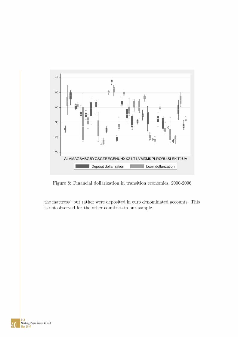
4.2 Descriptive Statistics

Figure 8 shows the variability and the median of dollarization over the sam-ple period for every country. Shaded bars represent 25-75 percentile of ob-servations, while vertical lines show the range of variation. The median isdenoted by a light line in the shaded bar. As can immediately be seen loanand deposit dollarization are not exactly two sides of the same coin. Thereare countries in our sample that have loan dollarization being higher thandeposit dollarization and vice versa. One can notice that there is a largevariation in dollarization for Serbia and Montenegro (CS) and Bosnia andHerzegovina (BA). This is explained by the fact that in CS as of June 2006around 80% of local currency loans had a foreign currency indexation clausethat linked repayments of principal and interest to the evolution of the di-nar exchange rate.24 It is suspected that something similar is happening inBA. Loan indexation is also prevalent in Croatia, but, we managed to obtainindexation adjusted data for this country. As indexation adjusted data andinterest rate data for BA and CS are not available these countries will notbe included in our empirical analysis.

Over time FD is evolving quite differently across countries (Figure 9).Loan dollarization is increasing in Bulgaria, Estonia, Hungary, Latvia, Poland,Slovenia and Slovakia, while deposit dollarization in these countries is fallingwith the exception of Latvia. It is also apparent that household loan dollar-ization is lower compared to firm dollarization (Table 4). This seems to betrue for all the countries except of Croatia and Latvia. Deposit dollarization,though being higher for households in general, is very much country specific.Long term loan dollarization is prevailing, while there is no clear distinctionbetween short term and long term deposit dollarization (short term beingdefined as less than one year).

For several countries in our sample we are able to estimate the share offoreign loans and deposits denominated in euro. The share of the euro amongforeign currency denominated loans is relatively high. With the exceptionof Bosnia and Herzegovina euro loan denomination is more frequent thandeposit euro denomination (Table 7).

The step change in deposit dollarization that can be observed in FYRMacedonia around January 2002 (Figure 9) can be explained by the eurocash changeover effect. As high levels of euro legacy currency holdings hadto be exchanged to euro, some holdings were no longer held in cash “under

24“Survey of Banks Business Activities and Intentions” National Bank of Serbia

35ECB


Table 4: Loan and deposit dollarization across countries (total, individ-ual/nonfinancial corporate, short term/long term, 2000-2006

Country ls tot ls ind ls nfc ls st ls lt ds tot ds ind ds nfc ds st ds ltAL 0.68 . . 0.64 0.77 0.31 0.26 0.54 0.47 0.2AM . . . . . 0.75 . . . .AZ 0.62 . . 0.59 0.69 0.59 0.89 0.38 . .BA 0.39 . . . . 0.52 . . 0.37 0.79BG 0.41 0.08 0.54 0.42 0.4 0.5 0.6 0.46 0.5 0.4BY . . . . . 0.57 0.51 0.63 0.59 0.56CS 0.35 0.06 0.41 0.17 0.51 0.63 0.78 0.48 0.63 0.66CZ 0.14 0.01 0.19 0.13 0.14 0.11 0.07 0.2 0.13 0EE 0.8 0.68 0.8 0.6 0.82 0.3 0.19 0.42 0.29 0.41GE 0.83 . . 0.75 0.91 0.94 . . 0.93 0.96HU 0.35 0.13 0.39 . . 0.17 0.15 0.21 0.18 0.01HR∗ 0.78 0.82 0.73 . . 0.65 0.79 0.36 . .KZ 0.57 . . . . 0.51 0.6 0.44 . .LT∗∗ 0.64 0.46 0.66 0.46 0.61 0.4 0.24 0.37 0.22 0.23LV 0.61 0.65 0.59 . . 0.41 0.44 0.37 . .MD 0.72 0.02 0.84 . . 0.5 . . . 0.5MK 0.2 0.01 0.24 0.14 0.27 0.48 0.66 0.29 . .PL 0.16 0.09 0.28 0.05 0.33 0.17 0.16 0.2 0.17 0.18RO 0.59 0.29 0.62 0.52 0.69 0.44 0.74 . . .RU 0.31 0.2 0.33 0.23 0.51 0.39 0.32 0.63 0.4 0.41SI 0.25 0.02 0.34 0.2 0.27 0.33 0.42 0.21 0.35 0.25SK 0.18 0.01 0.3 . . 0.15 0.13 0.19 0.39 .TJ 0.7 . . . . 0.57 0.81 0.47 . .UA 0.43 . . 0.35 0.53 0.35 . . 0.26 0.44Total 0.47 0.21 0.47 0.35 0.51 0.44 0.46 0.39 0.4 0.42

Source: National Central Banks∗ Adjusted for indexation∗∗ Split into short term/long term and individual/nonfinancial corporate is for euro denomina-tion only.


Table 5: Correlation of loan and deposit dollarization, 2000-2006

Country CorrelationAL 0.0778AZ -0.4538BA 0.7088BG -0.8201CS -0.8333CZ 0.6954EE -0.5933GE 0.8124HU -0.5577HR 0.8744KZ 0.7933LT 0.7076LV 0.6675MD 0.3912MK -0.2490PL -0.2843RO 0.4952RU 0.6850SI -0.0202SK -0.7123TJ -0.4376UA 0.7836Overall 0.5770

Source: National Central Banks

37ECB


Table 6: Correlation of ratio (1-2),foreign liabilities (3-4) and different mea-sures of foreign bank presence

Country sfb ta sfb nb sfb ta sfb nb(1) (2) (3) (4)

AL 0.9400 0.7512 0.9182 0.6865AM -0.2201 -0.1636 0.7988 0.9236AZ -0.4040 -0.0296 0.5166 0.7735BA -0.9375 -0.9584 -0.6011 -0.6448BG 0.7039 -0.2653 0.5422 0.3908BY 0.8743 0.8743 0.9117 0.8870CS -0.5649 -0.6833 0.0592 0.0079CZ -0.2718 -0.1547 -0.0432 0.1129EE 0.8610 0.8487 0.5376 0.7697GE -0.0911 0.0928 0.7208 0.7372HU -0.2277 -0.0528 0.3759 0.5745HR 0.1806 -0.0915 0.6630 0.4568KZ -0.1002 -0.9120 -0.2825 -0.6681LT 0.8196 0.7829 0.6004 0.4912LV 0.2590 0.4268 -0.3731 -0.2467MD -0.2634 -0.6053 0.3621 0.6646MK -0.1181 -0.2308 0.5741 0.4737PL 0.8888 0.9114 0.8845 0.9463RO 0.1753 0.2560 0.5398 0.5166RU 0.7631 0.4543 0.1403 0.7664SI 0.7598 0.8308 0.7438 0.8087SK 0.2735 0.2891 0.4895 0.4743TJ -0.2979 0.1361 -0.8437 0.9197UA -0.2188 0.4730 0.4682 0.5811Overall 0.2524 -0.0888 -0.0835 0.0820

Source: National Central Banks and EBRD

Table 7: Share of foreign loans and deposits denominated in euro, 2000-2006

Country ls eur ds eurAL 0.58 0.46BA 0.48 0.81BG 0.87 0.59CZ 0.68 0.64EE 0.91 0.4LT 0.76 0.48SK 0.74 0.63Total 0.7 0.58



Table 8: Interest rate differentials (on loans and deposits) and interest ratemargins(in foreign currency and local currency), 2000-2006

Country ir dif l ir dif d margi fc margi lcAL 6.30 4.95 5.49 6.83AM 0.22 2.59 15.11 12.74AZ -1.38 0.01 9.29 7.90BA . . . .BG 3.08 0.78 8.01 10.32BY 5.92 16.16 . .CS . . . .CZ 0.91 -0.16 1.86 2.81EE 2.12 0.07 2.24 4.04GE 2.24 -3.44 12.07 17.76HU 5.43 4.16 1.79 4.55HX 4.14 1.10 1.83 7.57KZ 3.23 0.87 9.23 11.59LT 1.51 -0.31 3.42 5.35LV 3.88 1.01 2.49 3.86MD 11.17 12.23 8.43 7.37MK 4.58 4.01 6.47 7.04PL 5.33 2.37 3.80 6.76RO 13.96 8.34 4.31 9.93RU 5.33 . . 10.79SI 3.07 1.78 2.90 5.17SK 1.27 0.65 1.41 2.01TJ 0.56 0.07 18.00 18.50UA 11.72 3.10 6.89 15.51Total 4.29 2.78 7.18 8.89


39ECB


0.2

.4.6

.81

ALAMAZBABGBYCSCZEEGEHUHXKZ LT LVMDMKPLRORU SI SK TJ UA

Deposit dollarization Loan dollarization

Figure 8: Financial dollarization in transition economies, 2000-2006

the mattress” but rather were deposited in euro denominated accounts. Thisis not observed for the other countries in our sample.


0.51 0.51 0.51 0.51 0.51

2000

m1

2002

m1

2004

m1

2006

m1 2

000m

120

02m

120

04m

120

06m

1 200

0m1

2002

m1

2004

m1

2006

m1

2000

m1

2002

m1

2004

m1

2006

m1 2

000m

120

02m

120

04m

120

06m

1

AL

AZ

BA

BG

CS

CZ

EE

GE

HU

HX

KZ

LTLV

MD

MK

PL

RO

RU

SI

SK

TJ

UA

Dep

osit

dolla

rizat

ion

Loan

dol

lariz

atio

n

Dat

e

Fig

ure

9:Fin

anci

aldol

lari

zati

on

41ECB


4.3 Methodology

Based on the existing literature and the implications of our theoretical modelwe estimate the following model:

shareit = β1ratioit + β2λit + β3ir difit + γmarginit + δmacroit + ci + eit (20)

Where share stands for dollarization (loans or deposits), ratio is the pro-portion of foreign currency denominated funds (as defined above, and whichaims to capture foreign bank penetration), ir dif stands for the interest dif-ferentials (loans and deposits) and margin stads for the interest rate margins(local currency and foreign currency). Finally, macro stands for the follow-ing macroeconomic controls: openness of the economy, exchange rate regime,and financial depth. After examination (Hausman specification test) fixedeffects are included to control for unobserved heterogeneity.

Equation 20 is estimated via FGLS with panel heteroscedasticity andpanel specific autocorrelation. Modified Wald test for groupwise heteroscedas-ticity rejects the null of σ2

i = σ2 and partial autocorrelation function of theerror term dies out quickly justifying AR1 structure for the error term.

Endogeneity of interest rate differentials and margins may be suspected.Formal endogeneity tests were not carried out due to the lack of properinstruments. However, to account for possible endogeneity the model is esti-mated using lagged values of interest rate differentials and margins. In anycase, estimation of the model based on the contemporaneous variables yieldsqualitatively similar results.

Four specifications of equation 20 are considered. First of all they differ inthe way λMV P is calculated. In the first specification we use lambda mue.25

In the second specification lambda mde is used.26 The third and fourth spec-ifications are estimated excluding currency board countries from the sample.

Tables 9 and 10 report regression results with the levels of dollarizationas dependent variables, while tables 11 and 12 report regression results withthe change in dollarization as a dependent variable. As our variables for FDare calculated using stock measures they can not capture well the changes inthe dollarization of the new loans and deposits. Since the measures of newbusiness activity are not available we proxy it by looking at the changes inthe stock variables.

25Using the euro/local currency exchange rate since 1999 and the USD/local currencyexchange rate prior to 1999.

26Using the euro/local currency exchange rate since 1999 and the DEM/local currencyexchange rate prior to 1999.


Regression results reported in columns 1 through 6 correspond to theuse of lambda mue and columns 7 through 12 correspond to the use oflambda mde. In the odd columns of the tables we report estimation re-sults where the dependent variable is loan dollarization, while in the evencolumns we report results for deposit dollarization. Estimations are carriedout for total (columns 1-2 and 7-8), individual (columns 3-4 and 9-10), andnonfinancial corporate dollarization (columns 5-6 and 11-12).

5 Estimation results

The main estimation results are reported in tables 9 through 12.

Share of funds in foreign currency

As predicted by the model, the share of funds in foreign currency (ratio)has a positive impact on loan dollarization and a negative impact on depositdollarization. This result is very robust across specifications. While ratio isfound to be very significant in explaining total and NFC loan and depositdollarization, it fails to explain loan dollarization by individuals.

Although we find that ratio has a positive effect on the change in loandollarization and a negative effect on the change in deposit dollarization byindividuals, overall significance of ratio explaining the change in dollariza-tion is minimal. This lends support to the explanation that the level ofdollarization is dependent on the share of foreign funds, while the variabilityaround that level is not. This is in line with the view that increased foreignbank presence in the region, by allowing banks to have greater access to for-eign funds, has contributed to loan dollarization. Consistent with our model,access to foreign funds leads to lower deposit dollarization.

Minimum variance portfolio dollarization

Estimation results confirm the theoretical argumentation of Ize and Levy-Yeyati (2003), incorporated into our model, that the level of dollarization isincreasing with the increase in λMV P . This results is quite robust no matterwhat measure of λMV P is being used. It must be noted, though, that thecoefficient appears to be negative for household and firm loan dollarization(but not for total) when the currency board countries are included in the

43ECB


sample (Table 9 columns 3, 5, and 9). This artifact disappears if the cur-rency board countries are dropped from the sample. As discussed above,theoretically, λMV P is not defined for currency board countries. It may beargued that λMV P should be dropped in case currency board countries areincluded, but then the model is misspecified with respect to non currencyboard countries. Tables 19 and 20 in the appendix show that the exclusionof λMV P in the regressions with currency board countries does not alter thequalitative results.

We also find that lambda mue has a positive impact on the change in loandollarization for all sectors of the economy. This holds both for the wholesample and when the currency board countries are dropped suggesting thatminimum variance portfolio argumentation is also relevant in explaining newloan dollarization.

Interest rate differentials

The estimation results suggest that interest rate differentials influence thecurrency composition of loans and deposits. Interest rate differentials havebetter explanatory power on changes in dollarization as compared to its level.

Estimation with the change in dollarization as a dependent variable yieldsconsistent results for all the specifications. The interest rate differential onloans has a positive effect on loan dollarization, while the interest rate differ-ential on deposits has a negative effect on deposit dollarization. This is in linewith the predictions of the model and appears to be the case for householdsand firms.

Analyzing the impact of interest rate differentials on the level of FD,we find that deposit dollarization of the individuals and firms is affectedby interest rate differential. It is higher when interest rate differential ondeposits is lower (Table 9 and 10). This is also consistent with our model.

The fact that interest rate differentials have almost no impact on thelevel of dollarization may be explained by the way we measure it. Theshare of foreign currency denominated loans and deposits being used in ourestimation is calculated from the stock variables, which naturally respondsless to interest rate differentials. Therefore, it is expected that interest ratedifferentials have stronger explanatory power on new businesses than on stockvariables.


Margins

The prediction of our model is that relation of margins to dollarization de-pends consistently on the parametrization of the model. In case banks carea lot about the loan market share relative to their market power, foreigncurrency margin and loan dollarization move in the same direction, whilelocal currency margin moves in the opposite direction (as share of funds inforeign currency changes). This would predict a positive sign on margin fcand a negative sign on margin lc in explaining loan dollarization. Signs fordeposit dollarization should be reversed.

However, empirical results on margins explaining the level of dollarizationdo not lend consistent support to the model implications. Increasing domes-tic margins seem to be decreasing loan dollarization, but this result is notrobust if currency board countries are excluded from the sample. Marginson foreign currency (margin fc) appear to have weak predicting power oryield contradicting results.

In the regressions with the change in dollarization as the dependent vari-able margins appear to have higher explanatory power. Local currency mar-gin decreases loan dollarization (as is predicted by the model in case 2).Deposit dollarization though, increases with margin fc (opposite of case 2).

One rationalization of this result is that in reality banks care not onlyabout loan market share (as is modeled), but also about deposit share. Thus,as the deposit market share becomes important, increasing domestic (foreign)margins should decrease (increase) dollarization of deposits (as is confirmedby regression results in Table 11 and 12).

This result can also be rationalized by the fact that in these economiesbank market power is comparatively high and banks are increasingly do-ing business in the currency with higher return. If local currency marginincreases, dollarization of deposits and loans decreases, while increasing for-eign currency margin has the opposite effect.

Macroeconomic conditions

In specifications with the level of FD as the dependent variable opennessof the economy is found to be increasing deposit dollarization, while at thesame time it is decreasing loan dollarization. If the currency board countriesare dropped from the sample openness looses significance in explaining loandollarization. However, openness has a positive impact for corporate loan and

45ECB


deposit dollarization with and without the currency board countries. Thisconfirms the implication of our model with firms and furthermore indicatesthat real dollarization contributes to FD.

The central bank intervention index (interv) has mostly no explanatorypower. For the few specifications where this variable is significant it seemsto have a negative impact on deposit dollarization.

Despite the fact that more interventions would lead to less variabilityin foreign exchange rate and therefore a shift towards dollarization, λMV P

is already capturing that effect as argued by Ize and Levy-Yeyati (2003).Hence the extra explanatory power of interventions could be coming fromthe increased confidence in local currency. This can be confirmed by thefact that when λMV P is excluded from the regression, intervention looses itssignificance (Table 19 and 20).

The signs of credit market depth (depth) coefficient seem to match withthe signs of the coefficients of the ratio variable (positive for loans and nega-tive for deposits). That leads us to conclude that domestic credit growth intransitional economies is mostly driven by the influx of foreign funds (throughthe increase in foreign liabilities).


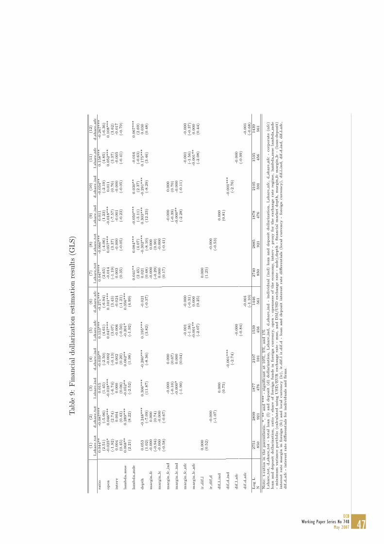
Tab

le9:

Fin

anci

aldol

lari

zati

ones

tim

atio

nre

sult

s(G

LS)

(1)

(2)

(3)

(4)

(5)

(6)

(7)

(8)

(9)

(10)

(11)

(12)

lsh

are

tot

dsh

are

tot

lsh

are

ind

dsh

are

ind

lsh

are

nfc

dsh

are

nfc

lsh

are

tot

dsh

are

tot

lsh

are

ind

dsh

are

ind

lsh

are

nfc

dsh

are

nfc

rati

o0.0

44**

-0.0

87***

0.0

15

-0.0

39**

0.1

53***

-0.2

71***

0.0

47***

-0.0

66***

0.0

11

-0.0

34**

0.1

58***

-0.2

67***

(2.5

1)

(-5.0

6)

(1.4

5)

(-2.5

0)

(4.6

1)

(-6.9

4)

(2.6

5)

(-4.0

6)

(1.2

3)

(-2.1

9)

(4.8

5)

(-6.3

6)

open

-0.0

25*

0.0

46***

-0.0

18***

-0.0

02

0.0

47***

0.1

01***

-0.0

14

0.0

57***

-0.0

18***

0.0

11

0.0

52***

0.1

08***

(-1.9

2)

(2.7

4)

(-6.7

4)

(-0.1

3)

(3.0

7)

(3.4

3)

(-1.1

9)

(3.3

7)

(-7.5

7)

(0.7

6)

(3.3

7)

(3.6

2)

inte

rv0.0

04

0.0

04

0.0

00

0.0

02

-0.0

06

-0.0

24

0.0

03

-0.0

00

-0.0

01

-0.0

00

-0.0

05

-0.0

17

(0.4

5)

(0.4

3)

(0.0

6)

(0.2

0)

(-0.5

0)

(-1.2

1)

(0.3

5)

(-0.0

5)

(-0.2

3)

(-0.0

5)

(-0.4

1)

(-0.7

9)

lam

bda

mue

0.0

68**

0.2

89***

-0.0

52**

0.0

62**

-0.2

01*

0.3

56***

(2.2

1)

(8.2

2)

(-2.5

2)

(1.9

8)

(-1.9

2)

(4.9

9)

lam

bda

mde

0.0

41**

0.0

84***

-0.0

50***

0.0

30**

-0.0

16

0.0

67***

(2.4

5)

(4.0

7)

(-3.1

1)

(2.3

7)

(-0.6

3)

(2.6

9)

depth

0.0

53

-0.2

48***

0.3

06***

-0.2

80***

0.1

95***

-0.0

21

0.0

21

-0.3

02***

0.3

03***

-0.2

91***

0.1

75***

0.0

30

(1.0

2)

(-7.0

9)

(11.8

7)

(-8.3

6)

(3.8

2)

(-0.3

7)

(0.4

8)

(-8.1

0)

(12.2

3)

(-8.2

9)

(3.4

6)

(0.4

8)

marg

infc

-0.0

00

0.0

00

-0.0

00

0.0

00

(-0.9

4)

(0.7

4)

(-0.2

9)

(0.9

0)

marg

inlc

-0.0

00

-0.0

00

0.0

00

-0.0

00

(-0.5

8)

(-0.6

7)

(0.1

7)

(-0.4

1)

marg

infc

ind

-0.0

00

0.0

00

-0.0

00

0.0

00

(-0.1

0)

(0.6

7)

(-0.3

9)

(0.7

0)

marg

inlc

ind

-0.0

00*

0.0

00

-0.0

00**

-0.0

00

(-1.9

0)

(0.0

4)

(-2.2

8)

(-0.1

1)

marg

infc

nfc

-0.0

01

-0.0

00

-0.0

01

-0.0

00

(-1.3

8)

(-0.3

1)

(-1.5

6)

(-0.3

7)

marg

inlc

nfc

-0.0

01**

0.0

00

-0.0

01**

0.0

00

(-2.0

7)

(0.2

5)

(-2.0

8)

(0.4

4)

irdif

l0.0

00

0.0

00

(0.5

2)

(1.2

5)

irdif

d-0

.000

-0.0

00

(-1.0

7)

(-0.5

3)

dif

lin

d0.0

00

0.0

00

(0.7

5)

(0.8

1)

dif

din

d-0

.001***

-0.0

01***

(-2.7

4)

(-2.7

6)

dif

lnfc

-0.0

00

-0.0

00

(-0.8

4)

(-0.9

9)

dif

dnfc

-0.0

01

-0.0

01

(-1.1

0)

(-0.6

8)

Log

L2751

2899

1877

2107

1539

1446

2740

2885

1878

2105

1535

1439

N850

921

476

591

456

561

850

921

476

591

456

561

Note

:t-

rati

os

inth

epare

nth

esi

s.*,**

and

***

-si

gnifi

cant

at

10%

,5%

,and

1%

lsh

are

tot,

dsh

are

tot

-to

tal

loan

(l)

and

deposi

t(d

)dollari

zati

on,

lsh

are

ind,

dsh

are

ind

-in

div

idual

(ind)

loan

and

deposi

tdollari

zati

on,

lsh

are

nfc

,d

share

nfc

-corp

ora

te(n

fc)

loan

and

deposi

tdollari

zati

on,ra

tio

-sh

are

of

fore

ign

funds

info

reig

ncurr

ency,open

-openness

of

the

econom

y,in

terv

-pro

xy

for

the

exchange

rate

regim

e,la

mbda

mue

lam

bda

mde

-m

inim

um

vari

ance

port

folio

(calc

ula

ted

usi

ng

USD

/EU

Rexchange

rate

-m

ue,and

DM

/U

SD

exchange

rate

-m

de),

depth

-financia

lm

ark

et

depth

,m

arg

infc

marg

inlc

-(l

oan-d

eposi

t)in

tere

stra

tem

arg

inin

fore

ign

(fc)

and

local

curr

ency

(lc),

irdif

lir

dif

d-

loan

and

deposi

tin

tere

stra

tediff

ere

nti

als

(local

curr

ency

-fo

reig

ncurr

ency),

dif

lin

d,

dif

din

d,

dif

lnfc

,dif

dnfc

-in

tere

stra

tediff

ere

nti

als

for

indiv

iduals

and

firm

s.

47ECB


Tab

le10

:Fin

anci

aldol

lari

zati

ones

tim

atio

nre

sult

s(G

LS):

dro

ppin

gcu

rren

cyboa

rdco

untr

ies

(1)

(2)

(3)

(4)

(5)

(6)

(7)

(8)

(9)

(10)

(11)

(12)

lsh

are

tot

dsh

are

tot

lsh

are

ind

dsh

are

ind

lsh

are

nfc

dsh

are

nfc

lsh

are

tot

dsh

are

tot

lsh

are

ind

dsh

are

ind

lsh

are

nfc

dsh

are

nfc

rati

o0.0

41**

-0.0

59***

-0.0

01

-0.0

22

0.0

62

-0.2

75***

0.0

51**

-0.0

56***

-0.0

02

-0.0

20

0.0

84**

-0.2

60***

(2.0

7)

(-3.2

0)

(-0.0

7)

(-1.0

8)

(1.4

3)

(-6.8

1)

(2.4

3)

(-2.9

5)

(-0.2

6)

(-1.0

0)

(2.0

3)

(-6.3

3)

open

-0.0

21

0.0

55***

-0.0

01

0.0

06

0.0

65***

0.0

65**

-0.0

15

0.0

81***

-0.0

02

0.0

15

0.0

67***

0.1

02***

(-1.5

2)

(2.8

1)

(-0.5

9)

(0.2

7)

(4.8

5)

(2.0

2)

(-1.0

8)

(4.1

0)

(-1.1

0)

(0.6

8)

(5.1

0)

(3.2

6)

inte

rv0.0

17

-0.0

05

0.0

01

-0.0

03

0.0

09

-0.0

53**

0.0

16

-0.0

19*

0.0

04

-0.0

01

0.0

09

-0.0

94***

(1.6

4)

(-0.4

2)

(0.2

9)

(-0.2

5)

(0.5

6)

(-2.4

5)

(1.6

3)

(-1.6

5)

(0.8

5)

(-0.0

9)

(0.5

5)

(-4.7

3)

lam

bda

mue

0.0

83***

0.1

99***

0.0

06

0.0

30

0.1

21

0.3

75***

(2.6

1)

(4.3

0)

(0.4

5)

(0.6

7)

(1.1

6)

(4.5

6)

lam

bda

mde

0.1

11***

0.1

25***

0.0

63***

0.0

54**

0.1

68***

0.0

94**

(4.0

4)

(4.8

4)

(3.7

1)

(2.0

5)

(3.8

0)

(2.4

5)

depth

-0.0

11

-0.1

81***

0.0

21

-0.5

11***

-0.1

33

0.0

65

-0.0

59

-0.3

75***

0.0

62***

-0.4

81***

-0.1

49*

0.1

89**

(-0.1

6)

(-2.7

0)

(1.3

5)

(-8.6

4)

(-1.4

9)

(0.8

0)

(-0.9

3)

(-6.2

1)

(2.8

8)

(-8.1

2)

(-1.8

9)

(2.3

3)

marg

infc

-0.0

00

0.0

00

-0.0

00

0.0

00

(-0.7

2)

(1.0

0)

(-0.6

7)

(1.1

4)

marg

inlc

-0.0

00

-0.0

00

0.0

00

-0.0

00

(-0.3

1)

(-0.8

6)

(0.1

4)

(-0.6

8)

marg

infc

ind

0.0

00

0.0

00

0.0

00

-0.0

00

(0.2

4)

(0.0

1)

(0.5

2)

(-0.0

5)

marg

inlc

ind

-0.0

00

-0.0

00

-0.0

00

-0.0

00

(-0.4

2)

(-1.1

9)

(-1.0

8)

(-1.0

1)

marg

infc

nfc

-0.0

00

0.0

01

-0.0

01

0.0

01

(-0.8

0)

(0.7

4)

(-0.9

6)

(0.8

8)

marg

inlc

nfc

-0.0

00

-0.0

02*

-0.0

00

-0.0

02*

(-0.7

5)

(-1.6

5)

(-0.6

0)

(-1.8

5)

irdif

l0.0

00

0.0

00

(0.7

6)

(0.8

3)

irdif

d-0

.000

-0.0

00

(-0.4

0)

(-0.1

7)

dif

lin

d0.0

00

0.0

00

(0.2

8)

(0.7

8)

dif

din

d-0

.001*

-0.0

01*

(-1.8

1)

(-1.8

4)

dif

lnfc

0.0

00

-0.0

00

(0.1

8)

(-0.3

7)

dif

dnfc

-0.0

03**

-0.0

03***

(-2.3

8)

(-2.7

2)

Log

L1968

2206

1381

1444

971

1027

1959

2187

1343

1455

974

1019

N625

696

307

422

281

388

625

696

307

422

281

388

Note

:t-

rati

os

inth

epare

nth

esi

s.*,**

and

***

-si

gnifi

cant

at

10%

,5%

,and

1%

lsh

are

tot,

dsh

are

tot

-to

tal

loan

(l)

and

deposi

t(d

)dollari

zati

on,

lsh

are

ind,

dsh

are

ind

-in

div

idual

(ind)

loan

and

deposi

tdollari

zati

on,

lsh

are

nfc

,d

share

nfc

-corp

ora

te(n

fc)

loan

and

deposi

tdollari

zati

on,ra

tio

-sh

are

of

fore

ign

funds

info

reig

ncurr

ency,open

-openness

of

the

econom

y,in

terv

-pro

xy

for

the

exchange

rate

regim

e,la

mbda

mue

lam

bda

mde

-m

inim

um

vari

ance

port

folio

(calc

ula

ted

usi

ng

USD

/EU

Rexchange

rate

-m

ue,and

DM

/U

SD

exchange

rate

-m

de),

depth

-financia

lm

ark

et

depth

,m

arg

infc

marg

inlc

-(l

oan-d

eposi

t)in

tere

stra

tem

arg

inin

fore

ign

(fc)

and

local

curr

ency

(lc),

irdif

lir

dif

d-

loan

and

deposi

tin

tere

stra

tediff

ere

nti

als

(local

curr

ency

-fo

reig

ncurr

ency),

dif

lin

d,

dif

din

d,

dif

lnfc

,dif

dnfc

-in

tere

stra

tediff

ere

nti

als

for

indiv

iduals

and

firm

s.


Tab

le11

:C

han

gein

finan

cial

dol

lari

zati

ones

tim

atio

nre

sult

s(G

LS)

(1)

(2)

(3)

(4)

(5)

(6)

(7)

(8)

(9)

(10)

(11)

(12)

∆lsh

tot

∆d

shto

t∆

lsh

ind

∆d

shin

d∆

lsh

nfc

∆d

shnfc

∆lsh

tot

∆d

shto

t∆

lsh

ind

∆d

shin

d∆

lsh

nfc

∆d

shnfc

rati

o0.0

20**

-0.0

04

0.0

02

-0.0

36***

0.0

02

-0.0

08

0.0

14*

-0.0

04

0.0

03

-0.0

37***

0.0

01

-0.0

07

(2.4

7)

(-0.4

8)

(0.5

1)

(-3.7

2)

(0.2

0)

(-0.3

3)

(1.8

0)

(-0.5

3)

(0.6

5)

(-3.7

9)

(0.1

0)

(-0.2

9)

open

0.0

01

-0.0

06*

0.0

03

0.0

03

0.0

04

-0.0

04

-0.0

00

-0.0

06*

0.0

03

0.0

03

0.0

05

-0.0

02

(0.2

9)

(-1.9

4)

(1.4

5)

(1.0

0)

(1.1

0)

(-0.4

1)

(-0.1

8)

(-1.9

5)

(1.2

8)

(0.9

3)

(1.1

5)

(-0.2

4)

inte

rv-0

.005*

0.0

04

0.0

06**

0.0

07*

0.0

01

0.0

05

-0.0

04

0.0

04

0.0

06***

0.0

07*

0.0

02

0.0

04

(-1.6

9)

(1.0

0)

(2.3

7)

(1.9

3)

(0.2

8)

(0.4

0)

(-1.4

4)

(1.0

1)

(2.7

5)

(1.9

2)

(0.3

7)

(0.3

4)

lam

bda

mue

0.0

20**

-0.0

03

0.0

18**

0.0

19**

0.0

51***

-0.0

05

(2.4

6)

(-0.3

7)

(2.1

4)

(2.0

3)

(3.5

4)

(-0.1

9)

lam

bda

mde

-0.0

04

-0.0

02

0.0

06

0.0

06*

0.0

07

-0.0

06

(-0.9

4)

(-0.6

8)

(1.3

9)

(1.8

6)

(1.4

4)

(-0.7

6)

depth

-0.0

16**

0.0

14

0.0

11*

0.0

06

-0.0

22**

0.0

06

-0.0

08

0.0

16

0.0

10

0.0

07

-0.0

13

0.0

10

(-2.3

8)

(1.4

1)

(1.7

7)

(0.8

0)

(-2.2

1)

(0.2

7)

(-1.2

4)

(1.5

3)

(1.5

9)

(0.9

4)

(-1.3

1)

(0.4

4)

marg

infc

0.0

00

0.0

01**

0.0

00

0.0

01**

(0.1

5)

(2.0

3)

(0.5

1)

(2.1

0)

marg

inlc

-0.0

00**

-0.0

00

-0.0

00

-0.0

00

(-2.1

3)

(-0.6

3)

(-1.5

3)

(-0.7

0)

marg

infc

ind

0.0

00

0.0

00

0.0

00

-0.0

00

(1.5

5)

(0.0

1)

(1.5

3)

(-0.0

8)

marg

inlc

ind

-0.0

00

-0.0

00

-0.0

00

-0.0

00

(-0.9

8)

(-1.4

9)

(-0.9

0)

(-1.1

6)

marg

infc

nfc

-0.0

00

0.0

01

0.0

00

0.0

01

(-0.2

4)

(1.1

4)

(0.0

6)

(1.2

2)

marg

inlc

nfc

-0.0

01

-0.0

00

-0.0

00

-0.0

00

(-1.5

7)

(-0.4

5)

(-1.3

2)

(-0.6

5)

irdif

l0.0

00

0.0

00

(0.9

1)

(1.1

3)

irdif

d-0

.001***

-0.0

01***

(-3.7

5)

(-3.6

8)

dif

lin

d0.0

00

0.0

00

(1.6

4)

(1.6

3)

dif

din

d-0

.001***

-0.0

01***

(-3.3

9)

(-3.3

5)

dif

lnfc

0.0

00**

0.0

01**

(1.9

6)

(2.2

5)

dif

dnfc

-0.0

02*

-0.0

01*

(-1.7

6)

(-1.6

9)

Log

L2797

2896

2207

2171

1625

1401

2796

2897

2201

2171

1620

1404

N846

917

475

586

455

556

846

917

475

586

455

556

Note

:t-

rati

os

inth

epare

nth

esi

s.*,**

and

***

-si

gnifi

cant

at

10%

,5%

,and

1%

∆lsh

tot,

∆d

shto

t-change

into

tallo

an

(l)

and

deposi

t(d

)dollari

zati

on,∆

lsh

ind,∆

dsh

ind

-change

inin

div

idual(i

nd)

loan

and

deposi

tdollari

zati

on,∆

lsh

nfc

,∆

dsh

nfc

-change

incorp

ora

te(n

fc)

loan

and

deposi

tdollari

zati

on,ra

tio

-sh

are

offo

reig

nfu

nds

info

reig

ncurr

ency,open

-openness

ofth

eeconom

y,in

terv

-pro

xy

for

the

exchange

rate

regim

e,la

mbda

mue

lam

bda

mde

-m

inim

um

vari

ance

port

folio

(calc

ula

ted

usi

ng

USD

/EU

Rexchange

rate

-m

ue,

and

DM

/U

SD

exchange

rate

-m

de),

depth

-financia

lm

ark

et

depth

,m

arg

infc

marg

inlc

-(l

oan-d

eposi

t)in

tere

stra

tem

arg

inin

fore

ign

(fc)

and

localcurr

ency

(lc),

irdif

lir

dif

d-lo

an

and

deposi

tin

tere

stra

tediff

ere

nti

als

(localcurr

ency

-fo

reig

ncurr

ency),

dif

lin

d,dif

din

d,

dif

lnfc

,dif

dnfc

-in

tere

stra

tediff

ere

nti

als

for

indiv

iduals

and

firm

s.

49ECB


Tab

le12

:C

han

gein

finan

cial

dol

lari

zati

ones

tim

atio

nre

sult

s(G

LS):

dro

ppin

gcu

rren

cyboa

rdco

untr

ies

(1)

(2)

(3)

(4)

(5)

(6)

(7)

(8)

(9)

(10)

(11)

(12)

∆lsh

tot

∆d

shto

t∆

lsh

ind

∆d

shin

d∆

lsh

nfc

∆d

shnfc

∆lsh

tot

∆d

shto

t∆

lsh

ind

∆d

shin

d∆

lsh

nfc

∆d

shnfc

rati

o0.0

12

-0.0

06

-0.0

02

-0.0

51***

0.0

22

0.0

05

0.0

12

-0.0

06

-0.0

01

-0.0

51***

0.0

16

-0.0

00

(1.1

4)

(-0.6

6)

(-0.3

7)

(-3.8

1)

(1.1

3)

(0.1

9)

(1.1

3)

(-0.6

6)

(-0.2

1)

(-3.7

8)

(0.8

1)

(-0.0

0)

open

0.0

00

-0.0

06*

0.0

05

-0.0

01

0.0

11*

-0.0

12

0.0

00

-0.0

06*

0.0

04

-0.0

02

0.0

08

-0.0

11

(0.0

3)

(-1.8

6)

(1.6

1)

(-0.2

8)

(1.8

9)

(-0.9

6)

(0.0

1)

(-1.8

5)

(1.4

6)

(-0.4

5)

(1.4

3)

(-0.8

8)

inte

rv-0

.009*

0.0

05

0.0

10***

0.0

03

-0.0

04

0.0

08

-0.0

08*

0.0

05

0.0

09***

0.0

01

-0.0

05

0.0

08

(-1.8

4)

(1.0

1)

(3.1

9)

(0.3

9)

(-0.5

5)

(0.3

7)

(-1.7

9)

(0.9

8)

(3.6

4)

(0.2

2)

(-0.6

4)

(0.4

0)

lam

bda

mue

0.0

22*

0.0

04

0.0

24**

0.0

15

0.0

66***

0.0

08

(1.7

9)

(0.4

2)

(2.0

9)

(0.8

4)

(2.8

5)

(0.2

0)

lam

bda

mde

0.0

14***

-0.0

00

0.0

14***

0.0

06

0.0

16**

-0.0

06

(2.7

3)

(-0.0

4)

(3.1

7)

(1.0

0)

(2.4

6)

(-0.5

5)

depth

-0.0

00

0.0

04

0.0

14

0.0

22

-0.0

45

-0.0

07

-0.0

10

0.0

08

0.0

06

0.0

21

-0.0

21

0.0

16

(-0.0

1)

(0.2

4)

(1.0

6)

(0.9

8)

(-1.5

0)

(-0.1

3)

(-0.5

4)

(0.4

7)

(0.4

4)

(0.9

6)

(-0.7

9)

(0.3

7)

marg

infc

0.0

00

0.0

01**

0.0

00

0.0

01**

(0.3

0)

(2.1

2)

(0.3

1)

(2.2

5)

marg

inlc

-0.0

01**

-0.0

00

-0.0

01**

-0.0

00

(-2.3

4)

(-1.1

0)

(-2.3

5)

(-1.0

1)

marg

infc

ind

0.0

00**

-0.0

00

0.0

00**

-0.0

00

(1.9

8)

(-0.0

3)

(2.0

8)

(-0.0

3)

marg

inlc

ind

-0.0

00

-0.0

00

-0.0

00

-0.0

00

(-1.0

2)

(-1.1

8)

(-0.9

1)

(-1.0

5)

marg

infc

nfc

-0.0

00

0.0

02*

-0.0

00

0.0

02*

(-0.1

4)

(1.7

8)

(-0.2

3)

(1.7

9)

marg

inlc

nfc

-0.0

01

-0.0

00

-0.0

01

-0.0

00

(-1.3

9)

(-0.4

5)

(-1.3

7)

(-0.5

2)

irdif

l0.0

00

0.0

00

(1.1

7)

(1.4

1)

irdif

d-0

.001***

-0.0

01***

(-3.8

6)

(-3.7

3)

dif

lin

d0.0

00**

0.0

00**

(2.1

2)

(2.1

9)

dif

din

d-0

.001***

-0.0

01***

(-3.3

8)

(-3.5

3)

dif

lnfc

0.0

01**

0.0

01***

(2.5

2)

(3.1

5)

dif

dnfc

-0.0

02**

-0.0

02**

(-2.3

6)

(-2.2

4)

Log

L2013

2214

1488

1508

1027

999

2016

2214

1493

1509

1027

1003

N621

692

307

418

281

384

621

692

307

418

281

384

Note

:t-

rati

os

inth

epare

nth

esi

s.*,**

and

***

-si

gnifi

cant

at

10%

,5%

,and

1%

∆lsh

tot,

∆d

shto

t-change

into

tallo

an

(l)

and

deposi

t(d

)dollari

zati

on,∆

lsh

ind,∆

dsh

ind

-change

inin

div

idual(i

nd)

loan

and

deposi

tdollari

zati

on,∆

lsh

nfc

,∆

dsh

nfc

-change

incorp

ora

te(n

fc)

loan

and

deposi

tdollari

zati

on,ra

tio

-sh

are

offo

reig

nfu

nds

info

reig

ncurr

ency,open

-openness

ofth

eeconom

y,in

terv

-pro

xy

for

the

exchange

rate

regim

e,la

mbda

mue

lam

bda

mde

-m

inim

um

vari

ance

port

folio

(calc

ula

ted

usi

ng

USD

/EU

Rexchange

rate

-m

ue,

and

DM

/U

SD

exchange

rate

-m

de),

depth

-financia

lm

ark

et

depth

,m

arg

infc

marg

inlc

-(l

oan-d

eposi

t)in

tere

stra

tem

arg

inin

fore

ign

(fc)

and

localcurr

ency

(lc),

irdif

lir

dif

d-lo

an

and

deposi

tin

tere

stra

tediff

ere

nti

als

(localcurr

ency

-fo

reig

ncurr

ency),

dif

lin

d,dif

din

d,

dif

lnfc

,dif

dnfc

-in

tere

stra

tediff

ere

nti

als

for

indiv

iduals

and

firm

s.


Sensitivity analysis

Table 13: Sensitivity analysis of country by country exclusionsDep. variable ratio open interv lambda depth margin fc margin lc ir difl share tot

looses significance AZCZLTMD

AZMDUA

gains significance EE AZEEHRUA

d share totlooses significance PLgains significance

∆ l share totlooses significance EE

GESI

ALGEHULTMKROSI

SI EE ROUA

gains significance GE

∆ d share totlooses significance CZ

MDSIUA

AM KZ

gains significance LT SI SK

We test the robustness of our results in a number of different ways. First,we used two different measures of λMV P and, as discussed, results are robustacross these two measures. Second, we estimated the model with and withoutthe currency board countries, which produced very similar results with theonly exception of λMV P .

Thirdly, because of better small sample properties we reestimate all ofthe above specifications of the model via OLS with heteroscedasticity andautocorrelation robust errors. OLS estimation results are presented in theappendix in Tables 15 and 18. The main qualitative results do not change.Note that, when explaining the level of household dollarization, interest ratedifferentials have the opposite sign compared to the model predictions, al-though impact on the change in dollarization remains the same.

Fourthly, we reestimate the empirical model for total dollarization of de-posits and loans (column 1 and 2 in Tables 9 and 11) dropping one countryat the time from the sample. None of the estimated parameters reverse signs,although some loose significance, while others gain. We report in Table 13countries for which their exclusion leads to these changes.

51ECB


In all the regressions lagged values for margin and ir dif are used. Thesame results are obtained when regressing on the contemporaneous variables(Tables 21 to 28 in the Appendix).

6 Conclusions

This paper develops a model to explain the determinants of financial dol-larization. Implications of the model are empirically verified using a newlycompiled data set on transition economies. We find that dollarization of de-posits is not generally matched by the dollarization of credit in contrast withthe model predictions of Ize (2005). For some countries in our sample creditdollarization is higher than deposit dollarization and vice versa.

The richness of our data set, split by households and firms as well as longterm and short term, allows us to explore financial dollarization in greatdetail. We observe that household credit dollarization is lower compared tocorporate dollarization, which might be comforting knowing that householdsusually have less hedging capabilities.

An important distinction between households and firms is that a country’sopenness to the international economy is contributing to corporate but not tohousehold financial dollarization, supporting the real dollarization paradigm.Note that the explanatory power of our model is generally lower for householdvis-a-vis total and corporate dollarization. Hence, this framework does notseem to capture all the main determinants of household dollarization andmore research is needed in this area.

We also find that long term credit dollarization is generally higher thanshort term credit dollarization. While short term credit dollarization carriesan increased risk of combining currency and maturity mismatches, the ex-change rate risk per se is higher in the case of foreign currency long-termcredit. This could be regarded as a potential vulnerability, as shocks to theexchange rate are expected to be more likely over a longer time span.

Our analysis nests the minimum variance portfolio framework. In linewith previous studies, the trade off between inflation and real exchange ratevariability is found to be a significant factor explaining financial dollarization.

One of the main features of transition economies is the increasing presenceof foreign banks and the consequent influx of foreign funds. According toour model, as well as the empirical results, access to foreign funds increasescredit dollarization although it decreases dollarization of deposits. This could


potentially increase currency mismatches in the agent’s portfolios in thesecountries, leading to higher credit risk (due to exchange risk) and a morefragile financial system. Thus, de-dollarization of credit could possibly beachieved by implementing controls on accumulation of net foreign liabilitiesin the banking sector. Note that even when credit and deposit dollarizationare matched at the aggregate level, there may be currency mismatches in theeconomy.

If uncovered interest rate parity holds then any interest rate differentialthat is observed on domestic and foreign currency denominated assets shouldbe explained by an expected depreciation or appreciation of the currency.Thus, interest rate differentials should not affect the currency compositionof loans and deposits.

In contrast with the literature we allow for uncovered interest rate paritynot to hold necessarily, hence the interest rate differential can play a part.Matching the implications of the model, our empirical results show that ahigher interest rate differential on loans increases credit dollarization. On theother hand, deposit dollarization decreases when the interest rate differentialon deposits increases. Hence interest rate differentials matter.

53ECB


Appendix A

An alternative specification of our model is when households choose at oncethe set (D, L, αd, αl), where D = total deposits, L = total loans, αd = por-tion of deposits in foreign currency (deposit dollarization) and αl = portion ofloans in foreign currency (loan dollarization), instead of splitting the house-holds into investors and fund managers. The other agents face the sameproblems.

We assume households maximize a Kreps-Porteus/Epstein-Zin utility func-tion allowing us to distinguish intertemporal elasticity of substitution(σ) anddegree of risk aversion (η) subject to period 1 and 2 budget constraints.

Formally household j ∈ H,L solves the following problem

max{C1,C2,D,L,αd,αl}

C1−1/σ1

1− 1/σ+ βj

[E

[C1−η

2

] 1−1/σ1−η

]

1− 1/σ

subject to

Y = C1 + D − L

Y = C2 − R̄dD + R̄lL

R̄d =

[Rd

p2

(1− αd) + e2R∗dαd

]

R̄l =

[Rl

p2

(1− αl) + e2R∗l αl

]

D = d + d∗, d = (1− αd)D and d∗ = αdD

L = l + l∗, l = (1− αl)L and l∗ = αlL

where R̄d and R̄l are the deposit and loan interest rates given by the weightedaverage of their respective rate indexes (formally defined in the aggrega-tor problem), (d, l) are the local currency denominated deposits and loans,(d∗, l∗) are the foreign currency denominated deposits and loans and p2 ande2 are price and real exchange rate at period 2, which are stochastic (periodone price and exchange rate are equal to 1). Main variables of interest areαd (deposit dollarization) and αl (loan dollarization).

The algorithm to solve this specification of the model with a single house-hold unit is very computationally intensive and therefore its solution for only


Table 14: Model Specification ComparisonAlternative Specification Main Specificationφ = 0.5 φ = 0.525 φ = 0.5 φ = 0.525

D 0.1095 0.109475 0.118977 0.118978αd 0.5 0.4940 0.5 0.495743L 0.1595 0.1595 0.168977 0.168978αl 0.5 0.504 0.5 0.5045Rd 1.1670 1.1675 1.17056 1.17077R∗

d 1.1670 1.6640 1.17056 1.17034Rl 1.2350 1.2355 1.23880 1.23902R∗

l 1.2350 1.2343 1.23880 1.23858

φ = 0.5 and φ = 0.525 are presented. The same parameter values shown intable 1 were used.

In addition we assume that η = 10, making sure differences in variancesand rates lead to portfolio diversification and that there are four possiblestates: both price and exchange rates are high (ph = 1.75,eh = 1.4285) withprobability 0.4, both price and exchange rate are low (pl = 0.7,el = 0.5715)with the same probability and the other two when one variable takes its highvalue and the other its low value, both with a probability of 0.1.

We then calculate the equilibrium of the model using the following gridsearch problem. Given a list of four rate indexes the household problems aresolved obtaining the aggregate demands. We then solve the bank problemusing the rate indexes and aggregate demands. The equilibrium rates areobtained when the rates chosen by the banks are equal to the four rateindexes. If no rate is found we increase the granularity of the grids.

Table 14 shows the results for both specifications of the model. Bothshowed the same patterns, as φ increases loan dollarization and interest ratedifferentials increase while deposit dollarization decreases. Note that L and Dare always lower in the alternative specification due to precautionary motivewhen variances are considered into the loans and deposits demand decision.Recall that due to the certainty equivalence assumption variances are notconsidered in that decision in the main specification of the model.

55ECB


Tab

le15

:Fin

anci

aldol

lari

zati

ones

tim

atio

nre

sult

s(O

LS

wit

hH

AC

robust

erro

rs)

(1)

(2)

(3)

(4)

(5)

(6)

(7)

(8)

(9)

(10)

(11)

(12)

lsh

are

tot

dsh

are

tot

lsh

are

ind

dsh

are

ind

lsh

are

nfc

dsh

are

nfc

lsh

are

tot

dsh

are

tot

lsh

are

ind

dsh

are

ind

lsh

are

nfc

dsh

are

nfc

rati

o0.0

18

-0.1

66***

0.1

53

-0.3

35***

0.5

06***

-0.4

04***

0.0

40

-0.1

21**

0.1

54

-0.3

28***

0.5

18***

-0.4

16***

(0.2

9)

(-3.3

6)

(1.6

1)

(-2.7

7)

(5.0

6)

(-5.9

1)

(0.6

6)

(-2.1

6)

(1.6

2)

(-2.7

4)

(5.3

7)

(-5.7

1)

open

-0.0

05

0.0

23

-0.0

54**

0.0

72***

0.0

77**

0.0

94**

0.0

06

0.0

41**

-0.0

56**

0.0

80***

0.0

85**

0.1

02**

(-0.2

2)

(1.3

0)

(-2.0

5)

(2.8

1)

(2.4

3)

(2.2

4)

(0.2

8)

(2.1

6)

(-2.1

1)

(3.2

3)

(2.5

8)

(2.2

4)

inte

rv0.0

38

0.0

06

0.0

55

-0.0

47

-0.1

17***

-0.0

17

0.0

61**

0.0

38

0.0

55

-0.0

41

-0.1

08***

-0.0

14

(1.4

2)

(0.2

2)

(1.0

6)

(-1.0

8)

(-3.0

3)

(-0.4

0)

(2.2

7)

(1.2

7)

(1.0

4)

(-0.9

1)

(-2.7

1)

(-0.3

4)

lam

bda

mue

0.2

33***

0.3

94***

-0.1

14

0.1

11

0.2

91*

0.2

91**

(3.4

0)

(10.0

3)

(-1.0

7)

(0.8

1)

(1.8

3)

(2.3

1)

lam

bda

mde

0.1

59***

0.1

79***

-0.0

08

0.0

88**

0.1

06*

0.0

72*

(3.8

3)

(4.9

8)

(-0.2

0)

(2.2

3)

(1.9

4)

(1.7

9)

depth

0.1

27**

-0.2

00***

0.1

54*

-0.3

10***

-0.1

58

0.0

10

0.0

50

-0.2

53***

0.1

24

-0.3

63***

-0.1

72*

0.0

28

(2.1

6)

(-3.2

4)

(1.7

4)

(-3.4

9)

(-1.5

8)

(0.1

4)

(0.8

0)

(-2.9

7)

(1.4

2)

(-3.8

3)

(-1.7

9)

(0.3

5)

marg

infc

-0.0

02

0.0

03**

-0.0

01

0.0

06***

(-1.0

2)

(2.2

9)

(-0.5

7)

(3.8

7)

marg

inlc

0.0

00

-0.0

01

0.0

00

0.0

00

(0.0

4)

(-1.3

6)

(0.2

5)

(0.2

0)

marg

infc

ind

-0.0

02

-0.0

03

-0.0

03

-0.0

03

(-1.2

2)

(-1.3

2)

(-1.3

9)

(-1.4

4)

marg

inlc

ind

-0.0

06**

0.0

02

-0.0

07**

0.0

02

(-2.0

1)

(0.8

7)

(-2.1

3)

(0.9

2)

marg

infc

nfc

-0.0

09***

-0.0

02

-0.0

09***

-0.0

02

(-2.8

2)

(-0.9

8)

(-3.0

5)

(-1.1

3)

marg

inlc

nfc

-0.0

07***

-0.0

03

-0.0

06**

-0.0

03

(-2.6

1)

(-1.4

6)

(-2.2

4)

(-1.3

0)

irdif

l0.0

01

0.0

01

(0.7

3)

(1.0

9)

irdif

d-0

.001

-0.0

01

(-1.5

2)

(-0.6

2)

dif

lin

d-0

.005**

-0.0

05**

(-2.3

5)

(-2.4

9)

dif

din

d0.0

06**

0.0

06**

(2.1

5)

(2.0

2)

dif

lnfc

0.0

03*

0.0

04**

(1.6

6)

(2.0

7)

dif

dnfc

-0.0

01

-0.0

01

(-0.6

9)

(-0.2

4)

Log

L1441

1882

957

1043

892

1038

1444

1813

956

1047

894

1031

N850

921

476

591

456

561

850

921

476

591

456

561

Note

:t-

rati

os

inth

epare

nth

esi

s.*,**

and

***

-si

gnifi

cant

at

10%

,5%

,and

1%

lsh

are

tot,

dsh

are

tot

-to

tal

loan

(l)

and

deposi

t(d

)dollari

zati

on,

lsh

are

ind,

dsh

are

ind

-in

div

idual

(ind)

loan

and

deposi

tdollari

zati

on,

lsh

are

nfc

,d

share

nfc

-corp

ora

te(n

fc)

loan

and

deposi

tdollari

zati

on,ra

tio

-sh

are

of

fore

ign

funds

info

reig

ncurr

ency,open

-openness

of

the

econom

y,in

terv

-pro

xy

for

the

exchange

rate

regim

e,la

mbda

mue

lam

bda

mde

-m

inim

um

vari

ance

port

folio

(calc

ula

ted

usi

ng

USD

/EU

Rexchange

rate

-m

ue,and

DM

/U

SD

exchange

rate

-m

de),

depth

-financia

lm

ark

et

depth

,m

arg

infc

marg

inlc

-(l

oan-d

eposi

t)in

tere

stra

tem

arg

inin

fore

ign

(fc)

and

local

curr

ency

(lc),

irdif

lir

dif

d-

loan

and

deposi

tin

tere

stra

tediff

ere

nti

als

(local

curr

ency

-fo

reig

ncurr

ency),

dif

lin

d,

dif

din

d,

dif

lnfc

,dif

dnfc

-in

tere

stra

tediff

ere

nti

als

for

indiv

iduals

and

firm

s.

Appendix B


Tab

le16

:Fin

anci

aldol

lari

zati

ones

tim

atio

nre

sult

s(O

LS

wit

hH

AC

robust

erro

rs):

dro

ppin

gcu

rren

cyboa

rdco

untr

ies (1

)(2

)(3

)(4

)(5

)(6

)(7

)(8

)(9

)(1

0)

(11)

(12)

lsh

are

tot

dsh

are

tot

lsh

are

ind

dsh

are

ind

lsh

are

nfc

dsh

are

nfc

lsh

are

tot

dsh

are

tot

lsh

are

ind

dsh

are

ind

lsh

are

nfc

dsh

are

nfc

rati

o-0

.006

-0.0

73

0.4

67***

-0.1

73

-0.0

62

-0.4

01***

0.0

60

-0.0

18

0.4

92***

-0.1

33

0.0

15

-0.4

14***

(-0.0

8)

(-1.3

9)

(3.2

6)

(-1.4

2)

(-0.5

4)

(-5.3

7)

(0.8

7)

(-0.3

4)

(3.7

1)

(-1.1

4)

(0.1

4)

(-5.7

5)

open

-0.0

11

0.0

36*

0.0

58

0.0

87**

0.0

68*

0.0

80*

0.0

10

0.0

59***

0.0

75**

0.0

94**

0.0

79**

0.0

81*

(-0.3

4)

(1.7

7)

(1.5

4)

(2.0

4)

(1.6

8)

(1.7

2)

(0.3

3)

(2.7

4)

(2.0

7)

(2.4

1)

(2.1

4)

(1.6

5)

inte

rv0.0

30

-0.0

82***

0.1

60**

-0.1

04

-0.0

16

-0.1

29*

0.0

28

-0.0

89***

0.1

59**

-0.1

22*

-0.0

26

-0.1

43**

(0.9

4)

(-2.9

4)

(2.5

0)

(-1.5

6)

(-0.4

0)

(-1.7

5)

(0.8

5)

(-3.3

2)

(2.4

7)

(-1.9

5)

(-0.6

3)

(-2.0

7)

lam

bda

mue

0.2

18**

0.4

18***

0.3

26***

0.3

69*

0.2

41

0.2

01

(2.1

6)

(6.6

7)

(2.6

3)

(1.6

9)

(1.4

9)

(1.2

2)

lam

bda

mde

0.2

85***

0.2

48***

0.1

96***

0.2

82***

0.2

24***

0.0

71

(4.2

3)

(5.3

3)

(4.1

0)

(4.1

4)

(3.2

9)

(1.3

7)

depth

0.0

17

-0.5

37***

-0.5

89**

-1.0

59***

0.5

92**

0.2

14

-0.3

21*

-0.5

69***

-0.7

33***

-1.2

70***

0.2

87

0.2

52

(0.0

7)

(-4.3

1)

(-2.4

6)

(-4.1

8)

(2.1

9)

(1.1

5)

(-1.7

6)

(-3.9

5)

(-3.4

9)

(-5.4

1)

(1.1

7)

(1.6

0)

marg

infc

-0.0

03

0.0

03**

-0.0

03*

0.0

05***

(-1.3

0)

(2.1

5)

(-1.7

6)

(3.1

9)

marg

inlc

0.0

01

-0.0

02**

0.0

01

-0.0

01

(0.6

2)

(-2.5

7)

(0.6

9)

(-1.2

4)

marg

infc

ind

-0.0

03

-0.0

02

-0.0

03

-0.0

02

(-1.2

3)

(-0.7

6)

(-1.1

6)

(-0.7

9)

marg

inlc

ind

-0.0

03

0.0

01

-0.0

00

0.0

01

(-1.0

8)

(0.3

0)

(-0.1

0)

(0.5

1)

marg

infc

nfc

0.0

09*

-0.0

01

0.0

05

-0.0

01

(1.7

5)

(-0.2

9)

(1.5

3)

(-0.4

2)

marg

inlc

nfc

0.0

01

-0.0

07***

0.0

02

-0.0

07***

(0.5

4)

(-2.8

8)

(0.9

5)

(-2.7

3)

irdif

l-0

.000

-0.0

01

(-0.0

5)

(-0.4

3)

irdif

d-0

.002*

-0.0

01

(-1.8

7)

(-0.8

5)

dif

lin

d-0

.005**

-0.0

05***

(-2.5

7)

(-2.7

7)

dif

din

d0.0

05

0.0

03

(1.6

0)

(1.0

8)

dif

lnfc

0.0

01

0.0

01

(0.3

6)

(0.5

2)

dif

dnfc

-0.0

04

-0.0

04

(-1.4

3)

(-1.2

8)

Log

L1019

1403

675

705

628

727

1038

1382

691

719

658

725

N625

696

307

422

281

388

625

696

307

422

281

388

Note

:t-

rati

os

inth

epare

nth

esi

s.*,**

and

***

-si

gnifi

cant

at

10%

,5%

,and

1%

lsh

are

tot,

dsh

are

tot

-to

tal

loan

(l)

and

deposi

t(d

)dollari

zati

on,

lsh

are

ind,

dsh

are

ind

-in

div

idual

(ind)

loan

and

deposi

tdollari

zati

on,

lsh

are

nfc

,d

share

nfc

-corp

ora

te(n

fc)

loan

and

deposi

tdollari

zati

on,ra

tio

-sh

are

of

fore

ign

funds

info

reig

ncurr

ency,open

-openness

of

the

econom

y,in

terv

-pro

xy

for

the

exchange

rate

regim

e,la

mbda

mue

lam

bda

mde

-m

inim

um

vari

ance

port

folio

(calc

ula

ted

usi

ng

USD

/EU

Rexchange

rate

-m

ue,and

DM

/U

SD

exchange

rate

-m

de),

depth

-financia

lm

ark

et

depth

,m

arg

infc

marg

inlc

-(l

oan-d

eposi

t)in

tere

stra

tem

arg

inin

fore

ign

(fc)

and

local

curr

ency

(lc),

irdif

lir

dif

d-

loan

and

deposi

tin

tere

stra

tediff

ere

nti

als

(local

curr

ency

-fo

reig

ncurr

ency),

dif

lin

d,

dif

din

d,

dif

lnfc

,dif

dnfc

-in

tere

stra

tediff

ere

nti

als

for

indiv

iduals

and

firm

s.

57ECB


Tab

le17

:C

han

gein

finan

cial

dol

lari

zati

ones

tim

atio

nre

sult

s(O

LS

wit

hH

AC

robust

erro

rs)

(1)

(2)

(3)

(4)

(5)

(6)

(7)

(8)

(9)

(10)

(11)

(12)

∆lsh

tot

∆d

shto

t∆

lsh

ind

∆d

shin

d∆

lsh

nfc

∆d

shnfc

∆lsh

tot

∆d

shto

t∆

lsh

ind

∆d

shin

d∆

lsh

nfc

∆d

shnfc

rati

o0.0

02

-0.0

14

-0.0

14

-0.0

70***

-0.0

15

-0.0

06

-0.0

01

-0.0

14

-0.0

15

-0.0

70***

-0.0

18

-0.0

08

(0.1

4)

(-1.0

9)

(-1.1

5)

(-3.7

4)

(-1.0

2)

(-0.2

4)

(-0.0

5)

(-1.1

0)

(-1.2

0)

(-3.7

0)

(-1.1

7)

(-0.3

2)

open

0.0

06

-0.0

12**

0.0

10**

-0.0

04

-0.0

01

-0.0

22

0.0

05

-0.0

12**

0.0

11**

-0.0

04

-0.0

01

-0.0

25

(0.4

1)

(-2.0

1)

(2.0

1)

(-0.5

4)

(-0.3

1)

(-1.1

1)

(0.3

3)

(-2.0

6)

(2.0

4)

(-0.5

4)

(-0.2

4)

(-1.1

5)

inte

rv-0

.011**

0.0

07

0.0

05

0.0

04

0.0

08

0.0

26

-0.0

09*

0.0

08

0.0

05

0.0

05

0.0

08

0.0

27

(-2.0

6)

(0.9

4)

(1.0

4)

(0.4

6)

(1.4

3)

(1.1

1)

(-1.7

1)

(0.9

6)

(0.9

8)

(0.5

2)

(1.4

5)

(1.0

9)

lam

bda

mue

0.0

13

0.0

03

0.0

20

0.0

25

0.0

36**

0.0

80

(0.8

2)

(0.2

5)

(1.6

0)

(0.9

5)

(2.0

3)

(1.2

4)

lam

bda

mde

-0.0

06

-0.0

00

-0.0

02

0.0

06

0.0

04

0.0

08

(-0.7

3)

(-0.0

4)

(-0.3

8)

(1.0

8)

(0.6

6)

(0.6

2)

depth

-0.0

02

0.0

24

0.0

19

0.0

18

-0.0

10

-0.0

04

0.0

07

0.0

25

0.0

28**

0.0

20

-0.0

01

0.0

13

(-0.1

6)

(1.5

3)

(1.5

0)

(1.1

3)

(-0.9

5)

(-0.1

5)

(0.4

8)

(1.4

7)

(2.0

8)

(1.2

2)

(-0.1

1)

(0.4

6)

marg

infc

0.0

01

0.0

00

0.0

01

0.0

00

(0.8

5)

(0.5

2)

(0.9

3)

(0.6

0)

marg

inlc

-0.0

01

0.0

00

-0.0

01

0.0

00

(-1.2

9)

(0.0

6)

(-1.1

4)

(0.1

3)

marg

infc

ind

0.0

01**

-0.0

01

0.0

01***

-0.0

01

(2.4

2)

(-0.7

2)

(2.7

4)

(-0.7

4)

marg

inlc

ind

-0.0

01**

-0.0

00

-0.0

01*

-0.0

00

(-2.0

6)

(-0.4

1)

(-1.7

9)

(-0.2

4)

marg

infc

nfc

-0.0

00

0.0

01

-0.0

00

0.0

01

(-0.8

1)

(0.6

9)

(-0.4

5)

(0.6

3)

marg

inlc

nfc

-0.0

01*

0.0

00

-0.0

01*

0.0

00

(-1.9

4)

(0.2

4)

(-1.8

0)

(0.4

4)

irdif

l0.0

00

0.0

00

(0.5

1)

(0.5

5)

irdif

d-0

.001***

-0.0

01***

(-3.0

6)

(-3.0

0)

dif

lin

d0.0

01***

0.0

01***

(3.0

2)

(3.1

4)

dif

din

d-0

.002***

-0.0

02**

(-2.6

3)

(-2.5

5)

dif

lnfc

0.0

01*

0.0

01**

(1.8

9)

(2.0

8)

dif

dnfc

-0.0

02

-0.0

01

(-1.1

0)

(-1.0

0)

Log

L1534

2471

1831

1766

1554

1246

1534

2471

1830

1766

1552

1245

N846

917

475

586

455

556

846

917

475

586

455

556

Note

:t-

rati

os

inth

epare

nth

esi

s.*,**

and

***

-si

gnifi

cant

at

10%

,5%

,and

1%

∆lsh

tot,

∆d

shto

t-change

into

tallo

an

(l)

and

deposi

t(d

)dollari

zati

on,∆

lsh

ind,∆

dsh

ind

-change

inin

div

idual(i

nd)

loan

and

deposi

tdollari

zati

on,∆

lsh

nfc

,∆

dsh

nfc

-change

incorp

ora

te(n

fc)

loan

and

deposi

tdollari

zati

on,ra

tio

-sh

are

offo

reig

nfu

nds

info

reig

ncurr

ency,open

-openness

ofth

eeconom

y,in

terv

-pro

xy

for

the

exchange

rate

regim

e,la

mbda

mue

lam

bda

mde

-m

inim

um

vari

ance

port

folio

(calc

ula

ted

usi

ng

USD

/EU

Rexchange

rate

-m

ue,

and

DM

/U

SD

exchange

rate

-m

de),

depth

-financia

lm

ark

et

depth

,m

arg

infc

marg

inlc

-(l

oan-d

eposi

t)in

tere

stra

tem

arg

inin

fore

ign

(fc)

and

localcurr

ency

(lc),

irdif

lir

dif

d-lo

an

and

deposi

tin

tere

stra

tediff

ere

nti

als

(localcurr

ency

-fo

reig

ncurr

ency),

dif

lin

d,dif

din

d,

dif

lnfc

,dif

dnfc

-in

tere

stra

tediff

ere

nti

als

for

indiv

iduals

and

firm

s.


Tab

le18

:C

han

gein

finan

cial

dol

lari

zati

ones

tim

atio

nre

sult

s(O

LS

wit

hH

AC

robust

erro

rs):

dro

ppin

gcu

rren

cyboa

rdco

untr

ies

(1)

(2)

(3)

(4)

(5)

(6)

(7)

(8)

(9)

(10)

(11)

(12)

∆lsh

tot

∆d

shto

t∆

lsh

ind

∆d

shin

d∆

lsh

nfc

∆d

shnfc

∆lsh

tot

∆d

shto

t∆

lsh

ind

∆d

shin

d∆

lsh

nfc

∆d

shnfc

rati

o0.0

00

-0.0

19

-0.0

21

-0.0

90***

-0.0

09

0.0

23

0.0

00

-0.0

18

-0.0

20

-0.0

89***

-0.0

13

0.0

08

(0.0

1)

(-1.1

3)

(-1.0

3)

(-3.9

0)

(-0.3

0)

(0.7

7)

(0.0

0)

(-1.0

7)

(-1.0

3)

(-3.9

0)

(-0.4

4)

(0.2

6)

open

0.0

07

-0.0

14**

0.0

14**

-0.0

19**

0.0

00

-0.0

38

0.0

08

-0.0

14**

0.0

15**

-0.0

18*

-0.0

01

-0.0

46

(0.3

6)

(-1.9

7)

(2.2

8)

(-2.1

1)

(0.0

5)

(-1.5

0)

(0.3

7)

(-1.9

9)

(2.4

4)

(-1.9

0)

(-0.2

0)

(-1.5

9)

inte

rv-0

.012*

0.0

10

0.0

12*

-0.0

06

0.0

03

0.0

64

-0.0

11

0.0

10

0.0

12*

-0.0

07

0.0

03

0.0

60

(-1.6

9)

(0.7

7)

(1.8

8)

(-0.3

8)

(0.3

7)

(1.2

0)

(-1.6

4)

(0.7

6)

(1.8

8)

(-0.3

8)

(0.3

2)

(1.1

2)

lam

bda

mue

0.0

26

0.0

19

0.0

28

-0.0

06

0.0

44

0.1

34

(0.8

6)

(0.7

4)

(1.5

5)

(-0.1

5)

(1.5

2)

(1.3

9)

lam

bda

mde

0.0

11

0.0

06

0.0

14**

0.0

01

0.0

14*

0.0

16

(0.6

6)

(0.5

2)

(2.4

7)

(0.1

3)

(1.8

4)

(0.7

5)

depth

-0.0

18

0.0

07

0.0

25

0.0

77*

-0.0

10

-0.0

93

-0.0

13

0.0

15

0.0

20

0.0

70*

0.0

05

-0.0

13

(-0.3

0)

(0.2

0)

(0.8

9)

(1.6

5)

(-0.2

3)

(-0.9

6)

(-0.2

4)

(0.3

9)

(0.8

0)

(1.8

0)

(0.1

4)

(-0.1

8)

marg

infc

0.0

01

0.0

00

0.0

01

0.0

01

(0.7

2)

(0.5

1)

(0.7

5)

(0.6

4)

marg

inlc

-0.0

01

-0.0

00

-0.0

01

-0.0

00

(-1.2

8)

(-0.3

5)

(-1.2

2)

(-0.0

4)

marg

infc

ind

0.0

01***

-0.0

01

0.0

01***

-0.0

01

(2.9

4)

(-0.7

5)

(3.0

9)

(-0.7

3)

marg

inlc

ind

-0.0

00

0.0

00

-0.0

00

0.0

00

(-1.6

0)

(0.0

9)

(-0.7

7)

(0.0

3)

marg

infc

nfc

-0.0

00

0.0

02

-0.0

01

0.0

02

(-0.6

9)

(1.5

9)

(-0.6

7)

(1.4

5)

marg

inlc

nfc

-0.0

01*

0.0

00

-0.0

01*

0.0

01

(-1.8

4)

(0.1

2)

(-1.7

5)

(0.5

3)

irdif

l0.0

00

0.0

00

(0.3

5)

(0.4

5)

irdif

d-0

.001***

-0.0

01***

(-2.9

5)

(-2.9

9)

dif

lin

d0.0

01***

0.0

01***

(3.3

2)

(3.3

5)

dif

din

d-0

.002***

-0.0

02***

(-2.6

4)

(-2.6

0)

dif

lnfc

0.0

01*

0.0

01**

(1.9

1)

(2.1

2)

dif

dnfc

-0.0

04**

-0.0

04**

(-2.4

2)

(-2.3

1)

Log

L1034

1816

1215

1206

962

857

1034

1815

1217

1206

962

856

N621

692

307

418

281

384

621

692

307

418

281

384

Note

:t-

rati

os

inth

epare

nth

esi

s.*,**

and

***

-si

gnifi

cant

at

10%

,5%

,and

1%

∆lsh

tot,

∆d

shto

t-change

into

tallo

an

(l)

and

deposi

t(d

)dollari

zati

on,∆

lsh

ind,∆

dsh

ind

-change

inin

div

idual(i

nd)

loan

and

deposi

tdollari

zati

on,∆

lsh

nfc

,∆

dsh

nfc

-change

incorp

ora

te(n

fc)

loan

and

deposi

tdollari

zati

on,ra

tio

-sh

are

offo

reig

nfu

nds

info

reig

ncurr

ency,open

-openness

ofth

eeconom

y,in

terv

-pro

xy

for

the

exchange

rate

regim

e,la

mbda

mue

lam

bda

mde

-m

inim

um

vari

ance

port

folio

(calc

ula

ted

usi

ng

USD

/EU

Rexchange

rate

-m

ue,

and

DM

/U

SD

exchange

rate

-m

de),

depth

-financia

lm

ark

et

depth

,m

arg

infc

marg

inlc

-(l

oan-d

eposi

t)in

tere

stra

tem

arg

inin

fore

ign

(fc)

and

localcurr

ency

(lc),

irdif

lir

dif

d-lo

an

and

deposi

tin

tere

stra

tediff

ere

nti

als

(localcurr

ency

-fo

reig

ncurr

ency),

dif

lin

d,dif

din

d,

dif

lnfc

,dif

dnfc

-in

tere

stra

tediff

ere

nti

als

for

indiv

iduals

and

firm

s.

59ECB


Tab

le19

:Fin

anci

aldol

lari

zati

ones

tim

atio

nre

sult

s(G

LS/H

AC

)

(1)

(2)

(3)

(4)

(5)

(6)

(7)

(8)

(9)

(10)

(11)

(12)

GLS

regre

ssio

nO

LS

HA

Ccorr

ecti

on

lsh

are

tot

dsh

are

tot

lsh

are

ind

dsh

are

ind

lsh

are

nfc

dsh

are

nfc

lsh

are

tot

dsh

are

tot

lsh

are

ind

dsh

are

ind

lsh

are

nfc

dsh

are

nfc

rati

o0.0

37**

-0.1

07***

0.0

08

-0.0

43***

0.1

48***

-0.2

74***

-0.0

12

-0.1

63***

0.1

56*

-0.3

42***

0.4

72***

-0.4

32***

(2.1

0)

(-5.2

2)

(0.7

7)

(-2.6

6)

(4.6

1)

(-6.4

0)

(-0.1

9)

(-2.8

0)

(1.6

6)

(-2.8

3)

(5.0

4)

(-5.7

8)

open

-0.0

13

0.0

38**

-0.0

18***

0.0

02

0.0

53***

0.1

23***

-0.0

10

0.0

28

-0.0

55**

0.0

71***

0.0

77**

0.0

95**

(-1.2

9)

(2.3

3)

(-7.0

7)

(0.1

4)

(3.2

9)

(4.1

9)

(-0.4

2)

(1.4

5)

(-2.0

9)

(2.9

6)

(2.4

0)

(2.0

4)

inte

rv-0

.002

0.0

04

0.0

00

-0.0

04

-0.0

05

-0.0

18

0.0

64**

0.0

37

0.0

55

-0.0

48

-0.1

18***

-0.0

24

(-0.2

2)

(0.3

5)

(0.0

0)

(-0.6

2)

(-0.4

4)

(-0.8

6)

(2.2

1)

(1.2

8)

(1.0

7)

(-1.1

1)

(-3.0

1)

(-0.5

7)

depth

0.0

04

-0.2

00***

0.2

93***

-0.2

66***

0.1

73***

0.1

11**

0.2

00***

-0.0

89

0.1

15

-0.2

74***

-0.0

48

0.0

98*

(0.0

9)

(-6.0

2)

(11.8

0)

(-8.3

0)

(3.4

1)

(2.2

1)

(3.2

3)

(-1.5

0)

(1.4

8)

(-4.0

6)

(-0.5

4)

(1.7

1)

marg

infc

0.0

00

0.0

00

-0.0

00

0.0

07***

(0.2

2)

(1.0

3)

(-0.1

9)

(4.3

4)

marg

inlc

0.0

00

0.0

00

0.0

01

0.0

01

(0.4

5)

(0.4

7)

(0.7

1)

(0.9

0)

marg

infc

ind

-0.0

00

0.0

00

-0.0

03

-0.0

03

(-0.2

9)

(0.8

0)

(-1.4

7)

(-1.3

0)

marg

inlc

ind

-0.0

01***

0.0

00

-0.0

07**

0.0

03

(-2.9

5)

(0.2

6)

(-2.1

4)

(1.0

2)

marg

infc

nfc

-0.0

01

-0.0

00

-0.0

07*

-0.0

02

(-1.4

2)

(-0.3

3)

(-1.9

4)

(-1.0

2)

marg

inlc

nfc

-0.0

01**

0.0

00

-0.0

06**

-0.0

03

(-2.0

4)

(0.2

8)

(-2.4

3)

(-1.2

8)

irdif

l0.0

01**

0.0

01

(2.1

3)

(1.1

4)

irdif

d0.0

00

-0.0

00

(0.2

6)

(-0.0

8)

dif

lin

d0.0

00

-0.0

05**

(1.2

1)

(-2.5

1)

dif

din

d-0

.001***

0.0

07**

(-2.7

4)

(2.4

0)

dif

lnfc

-0.0

00

0.0

04*

(-0.9

4)

(1.9

0)

dif

dnfc

-0.0

00

-0.0

00

(-0.3

8)

(-0.0

4)

Log

L2743

2869

1869

2102

1544

1437

1428

1769

956

1044

885

1030

N851

922

476

592

456

562

851

922

476

592

456

562

Note

:t-

rati

os

inth

epare

nth

esi

s.*,**

and

***

-si

gnifi

cant

at

10%

,5%

,and

1%

lsh

are

tot,

dsh

are

tot

-to

tal

loan

(l)

and

deposi

t(d

)dollari

zati

on,

lsh

are

ind,

dsh

are

ind

-in

div

idual

(ind)

loan

and

deposi

tdollari

zati

on,

lsh

are

nfc

,d

share

nfc

-corp

ora

te(n

fc)

loan

and

deposi

tdollari

zati

on,

rati

o-

share

of

fore

ign

funds

info

reig

ncurr

ency,

open

-openness

of

the

econom

y,

inte

rv-

pro

xy

for

the

exchange

rate

regim

e,

depth

-financia

lm

ark

et

depth

,m

arg

infc

marg

inlc

-(l

oan-d

eposi

t)in

tere

stra

tem

arg

inin

fore

ign

(fc)

and

localcurr

ency

(lc),

irdif

lir

dif

d-lo

an

and

deposi

tin

tere

stra

tediff

ere

nti

als

(localcurr

ency

-fo

reig

ncurr

ency),

dif

lin

d,dif

din

d,dif

lnfc

,dif

dnfc

-in

tere

stra

tediff

ere

nti

als

for

indiv

iduals

and

firm

s.


Tab

le20

:C

han

gein

finan

cial

dol

lari

zati

ones

tim

atio

nre

sult

s(G

LS/H

AC

)

(1)

(2)

(3)

(4)

(5)

(6)

(7)

(8)

(9)

(10)

(11)

(12)

GLS

regre

ssio

nO

LS

HA

Ccorr

ecti

on

∆lsh

tot

∆d

shto

t∆

lsh

ind

∆d

shin

d∆

lsh

nfc

∆d

shnfc

∆lsh

tot

∆d

shto

t∆

lsh

ind

∆d

shin

d∆

lsh

nfc

∆d

shnfc

rati

o0.0

17**

-0.0

03

0.0

02

-0.0

37***

-0.0

01

-0.0

05

0.0

01

-0.0

14

-0.0

14

-0.0

71***

-0.0

19

-0.0

09

(2.1

1)

(-0.4

1)

(0.5

3)

(-3.8

1)

(-0.0

7)

(-0.2

4)

(0.0

6)

(-1.0

9)

(-1.1

9)

(-3.7

7)

(-1.2

7)

(-0.3

8)

open

0.0

01

-0.0

06*

0.0

03

0.0

03

0.0

04

-0.0

03

0.0

05

-0.0

12**

0.0

11**

-0.0

05

-0.0

01

-0.0

26

(0.2

2)

(-1.9

3)

(1.3

3)

(0.8

3)

(0.9

3)

(-0.3

0)

(0.3

7)

(-2.0

0)

(2.0

7)

(-0.6

4)

(-0.3

0)

(-1.1

6)

inte

rv-0

.004

0.0

04

0.0

06**

0.0

07*

0.0

01

0.0

04

-0.0

09*

0.0

07

0.0

05

0.0

05

0.0

07

0.0

26

(-1.3

5)

(0.9

4)

(2.4

9)

(1.7

3)

(0.2

2)

(0.3

4)

(-1.7

3)

(0.9

3)

(1.0

0)

(0.4

6)

(1.4

0)

(1.0

6)

depth

-0.0

10*

0.0

12

0.0

12**

0.0

15**

-0.0

07

-0.0

00

0.0

02

0.0

25*

0.0

26**

0.0

26**

0.0

03

0.0

20

(-1.7

1)

(1.3

9)

(2.0

2)

(2.1

5)

(-0.7

4)

(-0.0

1)

(0.1

0)

(1.6

6)

(2.2

9)

(2.0

0)

(0.3

7)

(0.7

9)

marg

infc

0.0

00

0.0

01**

0.0

01

0.0

00

(0.5

9)

(2.0

1)

(0.9

2)

(0.6

1)

marg

inlc

-0.0

00

-0.0

00

-0.0

01

0.0

00

(-1.6

2)

(-0.7

1)

(-1.1

6)

(0.1

6)

marg

infc

ind

0.0

00*

0.0

00

0.0

01***

-0.0

01

(1.7

4)

(0.0

5)

(2.6

9)

(-0.7

4)

marg

inlc

ind

-0.0

00

-0.0

00

-0.0

01*

-0.0

00

(-0.8

9)

(-0.9

2)

(-1.7

9)

(-0.1

6)

marg

infc

nfc

0.0

00

0.0

01

-0.0

00

0.0

01

(0.1

8)

(1.1

4)

(-0.3

0)

(0.6

3)

marg

inlc

nfc

-0.0

00

-0.0

00

-0.0

01*

0.0

01

(-1.3

7)

(-0.5

9)

(-1.8

7)

(0.5

0)

irdif

l0.0

00

0.0

00

(1.0

7)

(0.5

5)

irdif

d-0

.001***

-0.0

01***

(-3.8

7)

(-3.0

2)

dif

lin

d0.0

00*

0.0

01***

(1.8

2)

(3.1

3)

dif

din

d-0

.001***

-0.0

02**

(-2.8

1)

(-2.5

0)

dif

lnfc

0.0

01**

0.0

01**

(2.2

0)

(2.0

6)

dif

dnfc

-0.0

02*

-0.0

01

(-1.9

3)

(-1.0

0)

Log

L2799

2898

2201

2169

1619

1406

1536

2472

1830

1769

1552

1247

N847

918

475

587

455

557

847

918

475

587

455

557

Note

:t-

rati

os

inth

epare

nth

esi

s.*,**

and

***

-si

gnifi

cant

at

10%

,5%

,and

1%

∆lsh

tot,

∆d

shto

t-

change

into

tallo

an

(l)

and

deposi

t(d

)dollari

zati

on,

∆lsh

ind,

∆d

shin

d-

change

inin

div

idual(i

nd)

loan

and

deposi

tdollari

zati

on,

∆lsh

nfc

,∆

dsh

nfc

-change

incorp

ora

te(n

fc)

loan

and

deposi

tdollari

zati

on,ra

tio

-sh

are

offo

reig

nfu

nds

info

reig

ncurr

ency,open

-openness

ofth

eeconom

y,in

terv

-pro

xy

for

the

exchange

rate

regim

e,la

mbda

mue

lam

bda

mde

-m

inim

um

vari

ance

port

folio

(calc

ula

ted

usi

ng

USD

/EU

Rexchange

rate

-m

ue,and

DM

/U

SD

exchange

rate

-m

de),

depth

-financia

lm

ark

et

depth

,m

arg

infc

marg

inlc

-(l

oan-d

eposi

t)in

tere

stra

tem

arg

inin

fore

ign

(fc)

and

localcurr

ency

(lc),

irdif

lir

dif

d-

loan

and

deposi

tin

tere

stra

tediff

ere

nti

als

(localcurr

ency

-fo

reig

ncurr

ency),

dif

lin

d,dif

din

d,dif

lnfc

,dif

dnfc

-in

tere

stra

tediff

ere

nti

als

for

indiv

iduals

and

firm

s.

61ECB


Tab

le21

:Fin

anci

aldol

lari

zati

ones

tim

atio

nre

sult

susi

ng

conte

mpor

aneo

us

inte

rest

rate

vari

able

s(G

LS)

(1)

(2)

(3)

(4)

(5)

(6)

(7)

(8)

(9)

(10)

(11)

(12)

lsh

are

tot

dsh

are

tot

lsh

are

ind

dsh

are

ind

lsh

are

nfc

dsh

are

nfc

lsh

are

tot

dsh

are

tot

lsh

are

ind

dsh

are

ind

lsh

are

nfc

dsh

are

nfc

rati

o0.0

40**

-0.0

76***

0.0

19*

-0.0

18

0.1

47***

-0.2

88***

0.0

46***

-0.0

65***

0.0

13

-0.0

15

0.1

46***

-0.2

80***

(2.4

6)

(-4.2

2)

(1.8

2)

(-1.3

4)

(4.7

1)

(-7.4

8)

(2.8

3)

(-3.5

6)

(1.3

4)

(-1.1

3)

(4.8

2)

(-6.6

0)

open

-0.0

22*

0.0

47***

-0.0

19***

-0.0

07

0.0

61***

0.0

77***

-0.0

14

0.0

54***

-0.0

20***

0.0

02

0.0

65***

0.0

72**

(-1.8

8)

(2.7

9)

(-6.9

7)

(-0.4

6)

(4.8

6)

(2.8

0)

(-1.2

5)

(3.2

5)

(-7.5

4)

(0.1

0)

(5.1

2)

(2.5

5)

inte

rv0.0

06

-0.0

07

0.0

02

-0.0

03

-0.0

16

-0.0

21

0.0

06

-0.0

11

0.0

02

-0.0

03

-0.0

13

0.0

03

(0.7

2)

(-0.7

0)

(0.3

5)

(-0.4

3)

(-1.2

8)

(-1.0

2)

(0.7

2)

(-1.0

8)

(0.3

7)

(-0.5

0)

(-1.1

0)

(0.1

2)

lam

bda

mue

0.0

52*

0.3

00***

-0.0

66***

0.0

36

-0.2

13**

0.2

78***

(1.9

0)

(8.7

6)

(-3.4

1)

(1.1

8)

(-2.3

1)

(4.0

3)

lam

bda

mde

0.0

33*

0.0

87***

-0.0

57***

0.0

24*

-0.0

15

0.0

71***

(1.8

9)

(4.3

4)

(-3.6

1)

(1.9

3)

(-0.6

1)

(2.9

7)

depth

0.0

93*

-0.2

55***

0.3

17***

-0.2

38***

0.2

32***

0.0

10

0.0

69

-0.3

13***

0.3

18***

-0.2

45***

0.2

14***

0.0

21

(1.7

8)

(-7.1

5)

(12.2

2)

(-6.8

4)

(4.7

2)

(0.1

7)

(1.4

7)

(-8.0

5)

(12.4

9)

(-6.6

7)

(4.2

9)

(0.3

3)

marg

infc

0.0

00

-0.0

00

0.0

01

-0.0

00

(1.3

6)

(-0.7

6)

(1.4

5)

(-0.7

5)

marg

inlc

0.0

01***

0.0

01*

0.0

01***

0.0

01**

(2.7

6)

(1.9

6)

(3.1

6)

(2.0

7)

marg

infc

ind

-0.0

00

0.0

00

-0.0

00

0.0

00

(-1.0

2)

(0.8

9)

(-1.3

6)

(0.8

2)

marg

inlc

ind

-0.0

00

0.0

00

-0.0

00*

0.0

00

(-1.6

1)

(1.4

4)

(-1.8

6)

(1.3

5)

marg

infc

nfc

0.0

00

-0.0

02***

0.0

00

-0.0

03***

(0.6

9)

(-2.5

8)

(0.6

2)

(-2.6

4)

marg

inlc

nfc

0.0

01

0.0

00

0.0

01

0.0

00

(1.4

2)

(0.4

4)

(1.4

5)

(0.4

9)

irdif

l0.0

01**

0.0

01**

(2.2

1)

(2.5

2)

irdif

d0.0

00

0.0

00

(0.4

1)

(1.0

9)

dif

lin

d0.0

00

0.0

00

(0.3

9)

(0.4

1)

dif

din

d0.0

00

0.0

00

(0.4

5)

(0.4

6)

dif

lnfc

0.0

01

0.0

01

(1.3

3)

(1.2

5)

dif

dnfc

0.0

00

0.0

00

(0.2

3)

(0.4

3)

Log

L2810

2919

1916

2159

1580

1478

2801

2909

1911

2158

1575

1476

N863

934

487

603

465

572

863

934

487

603

465

572

Note

:t-

rati

os

inth

epare

nth

esi

s.*,**

and

***

-si

gnifi

cant

at

10%

,5%

,and

1%

lsh

are

tot,

dsh

are

tot

-to

tal

loan

(l)

and

deposi

t(d

)dollari

zati

on,

lsh

are

ind,

dsh

are

ind

-in

div

idual

(ind)

loan

and

deposi

tdollari

zati

on,

lsh

are

nfc

,d

share

nfc

-corp

ora

te(n

fc)

loan

and

deposi

tdollari

zati

on,ra

tio

-sh

are

of

fore

ign

funds

info

reig

ncurr

ency,open

-openness

of

the

econom

y,in

terv

-pro

xy

for

the

exchange

rate

regim

e,la

mbda

mue

lam

bda

mde

-m

inim

um

vari

ance

port

folio

(calc

ula

ted

usi

ng

USD

/EU

Rexchange

rate

-m

ue,and

DM

/U

SD

exchange

rate

-m

de),

depth

-financia

lm

ark

et

depth

,m

arg

infc

marg

inlc

-(l

oan-d

eposi

t)in

tere

stra

tem

arg

inin

fore

ign

(fc)

and

local

curr

ency

(lc),

irdif

lir

dif

d-

loan

and

deposi

tin

tere

stra

tediff

ere

nti

als

(local

curr

ency

-fo

reig

ncurr

ency),

dif

lin

d,

dif

din

d,

dif

lnfc

,dif

dnfc

-in

tere

stra

tediff

ere

nti

als

for

indiv

iduals

and

firm

s.


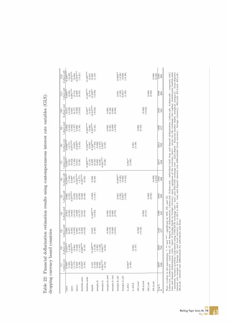
Tab

le22

:Fin

anci

aldol

lari

zati

ones

tim

atio

nre

sult

susi

ng

conte

mpor

aneo

us

inte

rest

rate

vari

able

s(G

LS):

dro

ppin

gcu

rren

cyboa

rdco

untr

ies

(1)

(2)

(3)

(4)

(5)

(6)

(7)

(8)

(9)

(10)

(11)

(12)

lsh

are

tot

dsh

are

tot

lsh

are

ind

dsh

are

ind

lsh

are

nfc

dsh

are

nfc

lsh

are

tot

dsh

are

tot

lsh

are

ind

dsh

are

ind

lsh

are

nfc

dsh

are

nfc

rati

o0.0

35*

-0.0

51**

0.0

00

-0.0

11

0.0

65

-0.2

78***

0.0

45**

-0.0

56***

-0.0

03

-0.0

11

0.0

80**

-0.2

46***

(1.9

3)

(-2.4

8)

(0.0

7)

(-0.5

6)

(1.5

5)

(-7.4

0)

(2.3

4)

(-2.7

1)

(-0.4

5)

(-0.5

9)

(2.0

0)

(-6.3

0)

open

-0.0

21*

0.0

55***

-0.0

01

-0.0

04

0.0

77***

0.0

49*

-0.0

16

0.0

71***

-0.0

02

0.0

04

0.0

81***

0.0

73***

(-1.7

1)

(2.8

4)

(-0.8

5)

(-0.1

5)

(4.9

2)

(1.7

7)

(-1.3

9)

(3.6

5)

(-1.2

7)

(0.1

7)

(5.1

5)

(2.6

6)

inte

rv0.0

16

-0.0

20

0.0

04

-0.0

09

0.0

10

-0.0

61***

0.0

15

-0.0

30**

0.0

06

-0.0

08

0.0

09

-0.0

74***

(1.5

8)

(-1.6

1)

(1.1

0)

(-0.7

7)

(0.5

8)

(-2.7

7)

(1.4

8)

(-2.4

5)

(1.3

4)

(-0.6

5)

(0.5

5)

(-3.2

1)

lam

bda

mue

0.0

53*

0.2

26***

-0.0

05

0.0

19

0.0

48

0.3

27***

(1.8

4)

(5.1

2)

(-0.4

3)

(0.4

4)

(0.4

6)

(4.3

6)

lam

bda

mde

0.0

83***

0.1

39***

0.0

55***

0.0

47*

0.1

29***

0.1

05***

(3.1

5)

(5.8

0)

(3.8

2)

(1.8

1)

(2.7

4)

(2.9

1)

depth

0.1

01

-0.2

29***

0.0

19

-0.4

30***

-0.0

94

0.0

38

0.0

29

-0.4

46***

0.0

57***

-0.4

15***

-0.1

66**

0.0

90

(1.4

4)

(-3.4

9)

(1.6

0)

(-6.8

5)

(-1.0

1)

(0.4

9)

(0.4

4)

(-7.8

4)

(3.4

4)

(-6.6

2)

(-2.0

9)

(1.1

0)

marg

infc

0.0

00

-0.0

01

0.0

00

-0.0

00

(0.9

5)

(-1.2

8)

(0.6

8)

(-0.9

7)

marg

inlc

0.0

01***

0.0

01**

0.0

01***

0.0

01*

(3.1

8)

(2.0

2)

(3.2

8)

(1.9

5)

marg

infc

ind

-0.0

00

0.0

00

0.0

00

0.0

00

(-0.1

9)

(0.4

3)

(0.4

5)

(0.4

6)

marg

inlc

ind

-0.0

00

0.0

00

-0.0

00

0.0

00

(-0.0

1)

(0.7

0)

(-0.6

3)

(0.6

6)

marg

infc

nfc

0.0

01

-0.0

03**

0.0

01

-0.0

03**

(1.2

6)

(-2.2

8)

(1.0

0)

(-2.3

8)

marg

inlc

nfc

0.0

01*

-0.0

00

0.0

01*

-0.0

00

(1.8

3)

(-0.4

3)

(1.9

3)

(-0.3

8)

irdif

l0.0

01*

0.0

01*

(1.8

5)

(1.6

8)

irdif

d0.0

01

0.0

01

(1.5

7)

(1.5

8)

dif

lin

d-0

.000

0.0

00

(-0.1

8)

(0.5

2)

dif

din

d0.0

00

-0.0

00

(0.1

1)

(-0.0

2)

dif

lnfc

0.0

00

0.0

00

(0.9

3)

(0.6

6)

dif

dnfc

-0.0

00

0.0

00

(-0.0

4)

(0.2

2)

Log

L2027

2225

1449

1498

1003

1056

2017

2214

1406

1505

1008

1050

N638

709

317

433

290

398

638

709

317

433

290

398

Note

:t-

rati

os

inth

epare

nth

esi

s.*,**

and

***

-si

gnifi

cant

at

10%

,5%

,and

1%

lsh

are

tot,

dsh

are

tot

-to

tal

loan

(l)

and

deposi

t(d

)dollari

zati

on,

lsh

are

ind,

dsh

are

ind

-in

div

idual

(ind)

loan

and

deposi

tdollari

zati

on,

lsh

are

nfc

,d

share

nfc

-corp

ora

te(n

fc)

loan

and

deposi

tdollari

zati

on,ra

tio

-sh

are

of

fore

ign

funds

info

reig

ncurr

ency,open

-openness

of

the

econom

y,in

terv

-pro

xy

for

the

exchange

rate

regim

e,la

mbda

mue

lam

bda

mde

-m

inim

um

vari

ance

port

folio

(calc

ula

ted

usi

ng

USD

/EU

Rexchange

rate

-m

ue,and

DM

/U

SD

exchange

rate

-m

de),

depth

-financia

lm

ark

et

depth

,m

arg

infc

marg

inlc

-(l

oan-d

eposi

t)in

tere

stra

tem

arg

inin

fore

ign

(fc)

and

local

curr

ency

(lc),

irdif

lir

dif

d-

loan

and

deposi

tin

tere

stra

tediff

ere

nti

als

(local

curr

ency

-fo

reig

ncurr

ency),

dif

lin

d,

dif

din

d,

dif

lnfc

,dif

dnfc

-in

tere

stra

tediff

ere

nti

als

for

indiv

iduals

and

firm

s.

63ECB


Tab

le23

:Fin

anci

aldol

lari

zati

ones

tim

atio

nre

sult

susi

ng

conte

mpor

aneo

us

inte

rest

rate

vari

able

s(O

LS

wit

hH

AC

robust

erro

rs)

(1)

(2)

(3)

(4)

(5)

(6)

(7)

(8)

(9)

(10)

(11)

(12)

lsh

are

tot

dsh

are

tot

lsh

are

ind

dsh

are

ind

lsh

are

nfc

dsh

are

nfc

lsh

are

tot

dsh

are

tot

lsh

are

ind

dsh

are

ind

lsh

are

nfc

dsh

are

nfc

rati

o0.0

15

-0.1

66***

0.1

71*

-0.3

02**

0.4

77***

-0.4

06***

0.0

38

-0.1

21**

0.1

71*

-0.2

95**

0.4

93***

-0.4

15***

(0.2

5)

(-3.4

1)

(1.8

0)

(-2.5

7)

(5.0

3)

(-6.1

4)

(0.6

3)

(-2.2

0)

(1.7

8)

(-2.5

3)

(5.3

9)

(-5.9

2)

open

-0.0

11

0.0

29

-0.0

53**

0.0

81***

0.0

80**

0.0

98**

0.0

01

0.0

44**

-0.0

54**

0.0

88***

0.0

87***

0.1

06**

(-0.4

7)

(1.6

2)

(-2.0

5)

(3.1

6)

(2.5

0)

(2.3

8)

(0.0

3)

(2.3

2)

(-2.0

9)

(3.5

5)

(2.6

6)

(2.3

8)

inte

rv0.0

40

-0.0

01

0.0

47

-0.0

52

-0.1

17***

-0.0

14

0.0

63**

0.0

31

0.0

48

-0.0

46

-0.1

06***

-0.0

11

(1.5

5)

(-0.0

3)

(0.9

4)

(-1.2

0)

(-3.0

6)

(-0.3

5)

(2.4

3)

(1.0

6)

(0.9

2)

(-1.0

4)

(-2.7

0)

(-0.2

6)

lam

bda

mue

0.2

28***

0.3

85***

-0.1

07

0.1

01

0.2

65*

0.2

89**

(3.4

1)

(9.5

6)

(-1.0

7)

(0.7

6)

(1.7

3)

(2.4

1)

lam

bda

mde

0.1

60***

0.1

75***

-0.0

04

0.0

80**

0.1

11**

0.0

75*

(3.8

5)

(4.9

6)

(-0.1

1)

(2.1

3)

(2.0

9)

(1.9

5)

depth

0.1

31**

-0.2

07***

0.1

36

-0.3

09***

-0.1

26

0.0

06

0.0

53

-0.2

54***

0.1

05

-0.3

57***

-0.1

56

0.0

23

(2.2

2)

(-3.2

8)

(1.5

1)

(-3.5

6)

(-1.2

8)

(0.0

9)

(0.8

4)

(-2.9

9)

(1.1

3)

(-3.9

1)

(-1.6

3)

(0.2

8)

marg

infc

-0.0

03

0.0

03**

-0.0

02

0.0

06***

(-1.4

1)

(2.4

4)

(-1.0

4)

(4.0

9)

marg

inlc

0.0

01

-0.0

01

0.0

01

0.0

00

(0.4

6)

(-1.5

6)

(0.7

0)

(0.2

4)

marg

infc

ind

-0.0

03

-0.0

01

-0.0

03

-0.0

02

(-1.4

0)

(-0.7

7)

(-1.5

7)

(-0.9

1)

marg

inlc

ind

-0.0

06*

0.0

02

-0.0

06*

0.0

02

(-1.7

9)

(0.8

4)

(-1.9

2)

(0.9

1)

marg

infc

nfc

-0.0

08**

-0.0

02

-0.0

08***

-0.0

02

(-2.4

2)

(-0.9

1)

(-2.7

1)

(-1.0

2)

marg

inlc

nfc

-0.0

06**

-0.0

04*

-0.0

06**

-0.0

04*

(-2.4

1)

(-1.9

4)

(-2.1

3)

(-1.7

0)

irdif

l0.0

01

0.0

01

(0.5

5)

(0.8

7)

irdif

d-0

.001

-0.0

00

(-0.7

3)

(-0.2

9)

dif

lin

d-0

.006***

-0.0

06***

(-2.6

5)

(-2.7

8)

dif

din

d0.0

08***

0.0

07***

(2.7

1)

(2.6

1)

dif

lnfc

0.0

03

0.0

04**

(1.6

3)

(2.0

5)

dif

dnfc

0.0

01

0.0

01

(0.3

3)

(0.7

0)

Log

L1463

1907

977

1068

903

1063

1467

1842

976

1071

906

1056

N863

934

487

603

465

572

863

934

487

603

465

572

Note

:t-

rati

os

inth

epare

nth

esi

s.*,**

and

***

-si

gnifi

cant

at

10%

,5%

,and

1%

lsh

are

tot,

dsh

are

tot

-to

tal

loan

(l)

and

deposi

t(d

)dollari

zati

on,

lsh

are

ind,

dsh

are

ind

-in

div

idual

(ind)

loan

and

deposi

tdollari

zati

on,

lsh

are

nfc

,d

share

nfc

-corp

ora

te(n

fc)

loan

and

deposi

tdollari

zati

on,ra

tio

-sh

are

of

fore

ign

funds

info

reig

ncurr

ency,open

-openness

of

the

econom

y,in

terv

-pro

xy

for

the

exchange

rate

regim

e,la

mbda

mue

lam

bda

mde

-m

inim

um

vari

ance

port

folio

(calc

ula

ted

usi

ng

USD

/EU

Rexchange

rate

-m

ue,and

DM

/U

SD

exchange

rate

-m

de),

depth

-financia

lm

ark

et

depth

,m

arg

infc

marg

inlc

-(l

oan-d

eposi

t)in

tere

stra

tem

arg

inin

fore

ign

(fc)

and

local

curr

ency

(lc),

irdif

lir

dif

d-

loan

and

deposi

tin

tere

stra

tediff

ere

nti

als

(local

curr

ency

-fo

reig

ncurr

ency),

dif

lin

d,

dif

din

d,

dif

lnfc

,dif

dnfc

-in

tere

stra

tediff

ere

nti

als

for

indiv

iduals

and

firm

s.


Tab

le24

:Fin

anci

aldol

lari

zati

ones

tim

atio

nre

sult

susi

ng

conte

mpor

aneo

us

inte

rest

rate

vari

able

s(O

LS

wit

hH

AC

robust

erro

rs):

dro

ppin

gcu

rren

cyboa

rdco

untr

ies

(1)

(2)

(3)

(4)

(5)

(6)

(7)

(8)

(9)

(10)

(11)

(12)

lsh

are

tot

dsh

are

tot

lsh

are

ind

dsh

are

ind

lsh

are

nfc

dsh

are

nfc

lsh

are

tot

dsh

are

tot

lsh

are

ind

dsh

are

ind

lsh

are

nfc

dsh

are

nfc

rati

o-0

.018

-0.0

72

0.4

64***

-0.1

44

-0.0

49

-0.3

96***

0.0

46

-0.0

21

0.4

98***

-0.1

14

0.0

25

-0.4

09***

(-0.2

4)

(-1.4

0)

(3.2

7)

(-1.2

1)

(-0.4

7)

(-5.5

9)

(0.6

6)

(-0.4

0)

(3.7

4)

(-1.0

0)

(0.2

4)

(-5.9

4)

open

-0.0

20

0.0

43**

0.0

59

0.0

97**

0.0

79*

0.1

02**

0.0

01

0.0

61***

0.0

78**

0.1

04***

0.0

89**

0.1

01**

(-0.6

3)

(2.0

5)

(1.5

4)

(2.2

2)

(1.9

7)

(2.2

2)

(0.0

3)

(2.8

0)

(2.1

0)

(2.6

3)

(2.5

0)

(2.1

1)

inte

rv0.0

35

-0.0

87***

0.1

49**

-0.0

96

-0.0

30

-0.1

09*

0.0

36

-0.0

91***

0.1

51**

-0.1

08*

-0.0

33

-0.1

21**

(1.1

4)

(-3.2

8)

(2.3

0)

(-1.5

6)

(-0.7

0)

(-1.6

5)

(1.1

2)

(-3.5

6)

(2.3

9)

(-1.8

3)

(-0.7

8)

(-1.9

8)

lam

bda

mue

0.1

93**

0.4

02***

0.3

11***

0.3

64*

0.2

39

0.2

04

(2.0

6)

(6.4

8)

(2.6

5)

(1.6

8)

(1.5

9)

(1.3

2)

lam

bda

mde

0.2

72***

0.2

36***

0.1

98***

0.2

58***

0.2

25***

0.0

71

(4.1

3)

(5.3

1)

(4.2

3)

(3.9

7)

(3.4

7)

(1.4

3)

depth

0.0

76

-0.5

28***

-0.6

06**

-1.0

42***

0.5

68**

0.1

62

-0.2

57

-0.5

47***

-0.7

65***

-1.2

04***

0.2

71

0.2

09

(0.3

4)

(-4.3

7)

(-2.5

4)

(-4.2

0)

(2.1

9)

(0.9

0)

(-1.4

0)

(-3.9

8)

(-3.6

3)

(-5.2

6)

(1.1

5)

(1.4

0)

marg

infc

-0.0

04

0.0

03**

-0.0

04**

0.0

05***

(-1.5

8)

(2.3

1)

(-2.0

6)

(3.4

5)

marg

inlc

0.0

02

-0.0

02***

0.0

02

-0.0

01

(1.0

8)

(-2.7

5)

(1.1

3)

(-1.1

9)

marg

infc

ind

-0.0

03

-0.0

00

-0.0

03

-0.0

00

(-1.2

5)

(-0.0

2)

(-1.1

7)

(-0.0

5)

marg

inlc

ind

-0.0

03

0.0

01

0.0

00

0.0

01

(-0.8

4)

(0.1

8)

(0.1

5)

(0.4

5)

marg

infc

nfc

0.0

10*

-0.0

01

0.0

07*

-0.0

02

(1.8

3)

(-0.5

9)

(1.7

3)

(-0.6

7)

marg

inlc

nfc

0.0

02

-0.0

08***

0.0

03*

-0.0

07***

(1.2

5)

(-3.3

8)

(1.7

4)

(-3.1

9)

irdif

l-0

.000

-0.0

01

(-0.1

1)

(-0.5

3)

irdif

d-0

.001

-0.0

01

(-1.1

7)

(-0.6

5)

dif

lin

d-0

.005***

-0.0

06***

(-2.9

2)

(-3.1

7)

dif

din

d0.0

06**

0.0

05*

(2.2

0)

(1.7

3)

dif

lnfc

-0.0

00

0.0

00

(-0.1

6)

(0.0

1)

dif

dnfc

0.0

00

0.0

01

(0.1

1)

(0.1

9)

Log

L1041

1431

690

728

643

750

1061

1413

708

740

675

748

N638

709

317

433

290

398

638

709

317

433

290

398

Note

:t-

rati

os

inth

epare

nth

esi

s.*,**

and

***

-si

gnifi

cant

at

10%

,5%

,and

1%

lsh

are

tot,

dsh

are

tot

-to

tal

loan

(l)

and

deposi

t(d

)dollari

zati

on,

lsh

are

ind,

dsh

are

ind

-in

div

idual

(ind)

loan

and

deposi

tdollari

zati

on,

lsh

are

nfc

,d

share

nfc

-corp

ora

te(n

fc)

loan

and

deposi

tdollari

zati

on,ra

tio

-sh

are

of

fore

ign

funds

info

reig

ncurr

ency,open

-openness

of

the

econom

y,in

terv

-pro

xy

for

the

exchange

rate

regim

e,la

mbda

mue

lam

bda

mde

-m

inim

um

vari

ance

port

folio

(calc

ula

ted

usi

ng

USD

/EU

Rexchange

rate

-m

ue,and

DM

/U

SD

exchange

rate

-m

de),

depth

-financia

lm

ark

et

depth

,m

arg

infc

marg

inlc

-(l

oan-d

eposi

t)in

tere

stra

tem

arg

inin

fore

ign

(fc)

and

local

curr

ency

(lc),

irdif

lir

dif

d-

loan

and

deposi

tin

tere

stra

tediff

ere

nti

als

(local

curr

ency

-fo

reig

ncurr

ency),

dif

lin

d,

dif

din

d,

dif

lnfc

,dif

dnfc

-in

tere

stra

tediff

ere

nti

als

for

indiv

iduals

and

firm

s.

65ECB


Tab

le25

:C

han

gein

finan

cial

dol

lari

zati

ones

tim

atio

nre

sult

susi

ng

conte

mpor

aneo

us

inte

rest

rate

vari

able

s(G

LS)

(1)

(2)

(3)

(4)

(5)

(6)

(7)

(8)

(9)

(10)

(11)

(12)

∆lsh

tot

∆d

shto

t∆

lsh

ind

∆d

shin

d∆

lsh

nfc

∆d

shnfc

∆lsh

tot

∆d

shto

t∆

lsh

ind

∆d

shin

d∆

lsh

nfc

∆d

shnfc

rati

o0.0

18**

-0.0

03

-0.0

00

-0.0

30***

0.0

09

-0.0

26

0.0

13

-0.0

03

0.0

02

-0.0

30***

0.0

10

-0.0

23

(2.1

5)

(-0.3

7)

(-0.0

2)

(-3.0

2)

(0.6

9)

(-1.1

7)

(1.6

0)

(-0.3

8)

(0.5

8)

(-3.0

9)

(0.7

5)

(-1.0

4)

open

-0.0

01

-0.0

07**

0.0

03

0.0

04

0.0

08**

-0.0

03

-0.0

02

-0.0

07**

0.0

02

0.0

03

0.0

08**

-0.0

02

(-0.3

2)

(-2.4

5)

(1.1

6)

(1.0

3)

(2.0

5)

(-0.3

7)

(-0.8

4)

(-2.4

7)

(0.7

5)

(0.9

3)

(2.1

6)

(-0.2

5)

inte

rv-0

.005

0.0

05

0.0

06***

0.0

07*

-0.0

00

0.0

08

-0.0

05*

0.0

05

0.0

06***

0.0

07*

0.0

01

0.0

08

(-1.5

1)

(1.2

1)

(2.6

3)

(1.7

3)

(-0.0

2)

(0.6

9)

(-1.6

6)

(1.2

5)

(3.4

8)

(1.8

1)

(0.1

3)

(0.7

3)

lam

bda

mue

0.0

08

-0.0

02

0.0

23***

0.0

16

0.0

46***

0.0

08

(0.8

8)

(-0.2

9)

(3.1

2)

(1.5

0)

(3.0

4)

(0.2

9)

lam

bda

mde

-0.0

07*

-0.0

02

0.0

07*

0.0

05

0.0

08*

0.0

00

(-1.7

2)

(-0.5

0)

(1.8

1)

(1.4

4)

(1.7

8)

(0.0

5)

depth

-0.0

15**

0.0

11

0.0

09

0.0

06

-0.0

22**

-0.0

03

-0.0

06

0.0

13

0.0

07

0.0

07

-0.0

16

-0.0

04

(-2.2

3)

(1.1

6)

(1.5

6)

(0.8

2)

(-2.1

3)

(-0.1

5)

(-0.8

8)

(1.2

3)

(1.2

9)

(0.9

0)

(-1.5

5)

(-0.1

7)

marg

infc

-0.0

00

-0.0

00

-0.0

00

-0.0

00

(-0.9

6)

(-0.3

2)

(-0.7

9)

(-0.3

3)

marg

inlc

-0.0

00

0.0

00

0.0

00

0.0

00

(-0.2

2)

(1.1

3)

(0.1

6)

(1.1

2)

marg

infc

ind

0.0

00

0.0

00

0.0

00

0.0

00

(0.2

7)

(0.3

9)

(0.2

1)

(0.3

1)

marg

inlc

ind

-0.0

00

-0.0

00

-0.0

00

-0.0

00

(-0.7

6)

(-0.6

4)

(-0.7

2)

(-0.4

0)

marg

infc

nfc

-0.0

00

-0.0

02**

-0.0

00

-0.0

02**

(-0.4

0)

(-2.2

1)

(-0.2

0)

(-2.1

7)

marg

inlc

nfc

0.0

00

0.0

00

0.0

00

0.0

00

(0.5

5)

(0.3

7)

(0.7

0)

(0.2

7)

irdif

l0.0

00

0.0

00

(0.6

0)

(0.6

5)

irdif

d-0

.001***

-0.0

01***

(-3.5

5)

(-3.5

1)

dif

lin

d0.0

00

0.0

00

(0.6

2)

(0.6

7)

dif

din

d-0

.001**

-0.0

01**

(-2.2

2)

(-2.3

3)

dif

lnfc

0.0

01***

0.0

01***

(3.1

0)

(3.3

8)

dif

dnfc

-0.0

01

-0.0

01

(-1.1

6)

(-1.1

5)

Log

L2824

2929

2237

2196

1646

1431

2823

2929

2234

2196

1643

1433

N855

926

484

596

462

565

855

926

484

596

462

565

Note

:t-

rati

os

inth

epare

nth

esi

s.*,**

and

***

-si

gnifi

cant

at

10%

,5%

,and

1%

∆lsh

tot,

∆d

shto

t-change

into

tallo

an

(l)

and

deposi

t(d

)dollari

zati

on,∆

lsh

ind,∆

dsh

ind

-change

inin

div

idual(i

nd)

loan

and

deposi

tdollari

zati

on,∆

lsh

nfc

,∆

dsh

nfc

-change

incorp

ora

te(n

fc)

loan

and

deposi

tdollari

zati

on,ra

tio

-sh

are

offo

reig

nfu

nds

info

reig

ncurr

ency,open

-openness

ofth

eeconom

y,in

terv

-pro

xy

for

the

exchange

rate

regim

e,la

mbda

mue

lam

bda

mde

-m

inim

um

vari

ance

port

folio

(calc

ula

ted

usi

ng

USD

/EU

Rexchange

rate

-m

ue,

and

DM

/U

SD

exchange

rate

-m

de),

depth

-financia

lm

ark

et

depth

,m

arg

infc

marg

inlc

-

(loan-d

eposi

t)in

tere

stra

tem

arg

inin

fore

ign

(fc)

and

localcurr

ency

(lc),

irdif

lir

dif

d-lo

an

and

deposi

tin

tere

stra

tediff

ere

nti

als

(localcurr

ency

-fo

reig

ncurr

ency),

dif

lin

d,dif

din

d,

dif

lnfc

,dif

dnfc

-in

tere

stra

tediff

ere

nti

als

for

indiv

iduals

and

firm

s.


Tab

le26

:C

han

gein

finan

cial

dol

lari

zati

ones

tim

atio

nre

sult

susi

ng

conte

mpor

aneo

us

inte

rest

rate

vari

able

s(G

LS):

dro

ppin

gcu

rren

cyboa

rdco

untr

ies

(1)

(2)

(3)

(4)

(5)

(6)

(7)

(8)

(9)

(10)

(11)

(12)

∆lsh

tot

∆d

shto

t∆

lsh

ind

∆d

shin

d∆

lsh

nfc

∆d

shnfc

∆lsh

tot

∆d

shto

t∆

lsh

ind

∆d

shin

d∆

lsh

nfc

∆d

shnfc

rati

o0.0

11

-0.0

07

-0.0

04

-0.0

47***

0.0

26

-0.0

28

0.0

13

-0.0

06

-0.0

02

-0.0

47***

0.0

22

-0.0

26

(0.9

5)

(-0.6

9)

(-0.5

7)

(-3.5

8)

(1.3

1)

(-1.0

4)

(1.1

5)

(-0.5

9)

(-0.5

2)

(-3.5

1)

(1.1

0)

(-1.0

3)

open

-0.0

02

-0.0

08**

0.0

05

-0.0

03

0.0

14**

-0.0

10

-0.0

02

-0.0

08**

0.0

03

-0.0

03

0.0

11*

-0.0

09

(-0.6

6)

(-2.3

7)

(1.2

8)

(-0.5

2)

(2.3

6)

(-0.8

6)

(-0.5

1)

(-2.3

3)

(0.7

9)

(-0.6

6)

(1.9

4)

(-0.8

0)

inte

rv-0

.009*

0.0

05

0.0

09***

0.0

01

-0.0

02

0.0

12

-0.0

09*

0.0

05

0.0

09***

0.0

00

-0.0

02

0.0

14

(-1.8

3)

(1.0

2)

(2.7

4)

(0.1

1)

(-0.2

6)

(0.5

5)

(-1.8

2)

(1.0

1)

(3.7

1)

(0.0

3)

(-0.3

5)

(0.7

2)

lam

bda

mue

0.0

11

0.0

04

0.0

33***

0.0

13

0.0

65***

0.0

04

(0.8

8)

(0.3

5)

(2.6

9)

(0.6

8)

(2.7

7)

(0.1

1)

lam

bda

mde

0.0

12**

-0.0

00

0.0

15***

0.0

07

0.0

15**

-0.0

03

(2.0

3)

(-0.0

2)

(3.4

1)

(1.0

6)

(2.3

3)

(-0.2

2)

depth

0.0

04

0.0

07

0.0

09

0.0

23

-0.0

48

0.0

13

-0.0

06

0.0

09

0.0

02

0.0

19

-0.0

26

0.0

18

(0.2

0)

(0.4

5)

(0.6

2)

(1.0

2)

(-1.6

0)

(0.2

6)

(-0.3

1)

(0.5

5)

(0.1

5)

(0.9

0)

(-0.9

8)

(0.4

1)

marg

infc

-0.0

00

-0.0

00

-0.0

00

-0.0

00

(-1.1

1)

(-0.5

5)

(-1.1

5)

(-0.4

6)

marg

inlc

-0.0

00

0.0

00

-0.0

00

0.0

00

(-0.3

8)

(0.6

1)

(-0.3

3)

(0.7

6)

marg

infc

ind

0.0

00

0.0

00

0.0

00

0.0

00

(0.2

6)

(0.4

0)

(0.6

7)

(0.4

4)

marg

inlc

ind

-0.0

00

-0.0

00

-0.0

00

-0.0

00

(-0.5

4)

(-0.3

6)

(-0.6

8)

(-0.2

2)

marg

infc

nfc

-0.0

00

-0.0

02*

-0.0

00

-0.0

02*

(-0.2

6)

(-1.7

5)

(-0.3

8)

(-1.7

1)

marg

inlc

nfc

-0.0

00

0.0

00

-0.0

00

0.0

00

(-0.2

2)

(0.4

1)

(-0.2

7)

(0.3

4)

irdif

l0.0

00

0.0

00

(0.3

2)

(0.2

8)

irdif

d-0

.001***

-0.0

01***

(-3.2

9)

(-3.2

5)

dif

lin

d0.0

00

0.0

00

(0.3

0)

(0.7

4)

dif

din

d-0

.001***

-0.0

01***

(-2.9

3)

(-3.0

3)

dif

lnfc

0.0

01***

0.0

01***

(3.0

6)

(3.6

9)

dif

dnfc

-0.0

02

-0.0

02

(-1.5

4)

(-1.5

1)

Log

L2035

2243

1516

1533

1047

1023

2037

2244

1526

1533

1046

1026

N630

701

315

427

288

392

630

701

315

427

288

392

Note

:t-

rati

os

inth

epare

nth

esi

s.*,**

and

***

-si

gnifi

cant

at

10%

,5%

,and

1%

∆lsh

tot,

∆d

shto

t-change

into

tallo

an

(l)

and

deposi

t(d

)dollari

zati

on,∆

lsh

ind,∆

dsh

ind

-change

inin

div

idual(i

nd)

loan

and

deposi

tdollari

zati

on,∆

lsh

nfc

,∆

dsh

nfc

-change

incorp

ora

te(n

fc)

loan

and

deposi

tdollari

zati

on,ra

tio

-sh

are

offo

reig

nfu

nds

info

reig

ncurr

ency,open

-openness

ofth

eeconom

y,in

terv

-pro

xy

for

the

exchange

rate

regim

e,la

mbda

mue

lam

bda

mde

-m

inim

um

vari

ance

port

folio

(calc

ula

ted

usi

ng

USD

/EU

Rexchange

rate

-m

ue,

and

DM

/U

SD

exchange

rate

-m

de),

depth

-financia

lm

ark

et

depth

,m

arg

infc

marg

inlc

-(l

oan-d

eposi

t)in

tere

stra

tem

arg

inin

fore

ign

(fc)

and

localcurr

ency

(lc),

irdif

lir

dif

d-lo

an

and

deposi

tin

tere

stra

tediff

ere

nti

als

(localcurr

ency

-fo

reig

ncurr

ency),

dif

lin

d,dif

din

d,

dif

lnfc

,dif

dnfc

-in

tere

stra

tediff

ere

nti

als

for

indiv

iduals

and

firm

s.

67ECB


Tab

le27

:C

han

gein

finan

cial

dol

lari

zati

ones

tim

atio

nre

sult

susi

ng

conte

mpor

aneo

us

inte

rest

rate

vari

able

s(O

LS

wit

hH

AC

robust

erro

rs)

(1)

(2)

(3)

(4)

(5)

(6)

(7)

(8)

(9)

(10)

(11)

(12)

∆lsh

tot

∆d

shto

t∆

lsh

ind

∆d

shin

d∆

lsh

nfc

∆d

shnfc

∆lsh

tot

∆d

shto

t∆

lsh

ind

∆d

shin

d∆

lsh

nfc

∆d

shnfc

rati

o-0

.002

-0.0

18

-0.0

11

-0.0

73***

0.0

01

-0.0

22

-0.0

04

-0.0

17

-0.0

12

-0.0

73***

0.0

00

-0.0

24

(-0.1

1)

(-1.3

2)

(-0.9

9)

(-3.6

4)

(0.0

9)

(-0.9

3)

(-0.2

8)

(-1.2

7)

(-1.0

0)

(-3.6

0)

(0.0

4)

(-0.9

8)

open

-0.0

02

-0.0

16**

0.0

09*

-0.0

04

0.0

07

-0.0

25

-0.0

03

-0.0

16**

0.0

10*

-0.0

04

0.0

07

-0.0

27

(-0.2

1)

(-2.4

3)

(1.8

7)

(-0.6

1)

(1.4

6)

(-1.2

6)

(-0.3

0)

(-2.4

5)

(1.9

2)

(-0.6

0)

(1.5

1)

(-1.2

7)

inte

rv-0

.006

0.0

08

0.0

07

0.0

03

0.0

05

0.0

28

-0.0

05

0.0

09

0.0

07

0.0

04

0.0

05

0.0

30

(-1.0

5)

(1.0

4)

(1.3

8)

(0.3

1)

(0.9

1)

(1.2

0)

(-0.9

3)

(1.1

0)

(1.3

4)

(0.3

7)

(0.9

7)

(1.2

0)

lam

bda

mue

0.0

05

0.0

08

0.0

25**

0.0

25

0.0

25

0.0

76

(0.2

8)

(0.5

3)

(2.2

2)

(0.9

1)

(1.4

2)

(1.2

7)

lam

bda

mde

-0.0

07

0.0

02

-0.0

00

0.0

07

0.0

05

0.0

11

(-0.8

4)

(0.2

8)

(-0.0

7)

(1.0

8)

(0.8

9)

(0.8

7)

depth

-0.0

02

0.0

22

0.0

15

0.0

16

-0.0

08

-0.0

04

0.0

06

0.0

22

0.0

24*

0.0

17

-0.0

05

0.0

08

(-0.1

5)

(1.3

2)

(1.1

6)

(0.9

7)

(-0.7

4)

(-0.1

7)

(0.4

0)

(1.2

4)

(1.7

8)

(0.9

9)

(-0.4

1)

(0.3

0)

marg

infc

-0.0

01

-0.0

01

-0.0

01

-0.0

01

(-0.8

6)

(-0.6

9)

(-0.8

2)

(-0.6

7)

marg

inlc

0.0

00

0.0

00

0.0

00

0.0

00

(0.4

5)

(1.3

9)

(0.5

6)

(1.4

8)

marg

infc

ind

0.0

01**

-0.0

01

0.0

01**

-0.0

01

(2.2

0)

(-1.1

7)

(2.5

3)

(-1.1

8)

marg

inlc

ind

-0.0

01**

-0.0

00

-0.0

01*

0.0

00

(-2.2

9)

(-0.0

8)

(-1.9

5)

(0.0

8)

marg

infc

nfc

-0.0

00

-0.0

01

-0.0

00

-0.0

01

(-0.3

7)

(-0.7

4)

(-0.2

3)

(-0.8

1)

marg

inlc

nfc

0.0

00

0.0

01

0.0

00

0.0

01

(0.9

2)

(0.8

1)

(1.0

2)

(1.0

1)

irdif

l0.0

00

0.0

00

(0.3

6)

(0.3

7)

irdif

d-0

.001***

-0.0

01***

(-2.8

7)

(-2.8

2)

dif

lin

d0.0

01***

0.0

01***

(2.8

5)

(2.9

9)

dif

din

d-0

.002***

-0.0

02**

(-2.6

0)

(-2.5

8)

dif

lnfc

0.0

01***

0.0

01***

(3.3

5)

(3.5

6)

dif

dnfc

-0.0

02

-0.0

02

(-1.5

9)

(-1.5

3)

Log

L1555

2503

1855

1801

1581

1272

1555

2503

1853

1801

1580

1271

N855

926

484

596

462

565

855

926

484

596

462

565

Note

:t-

rati

os

inth

epare

nth

esi

s.*,**

and

***

-si

gnifi

cant

at

10%

,5%

,and

1%

∆lsh

tot,

∆d

shto

t-change

into

tallo

an

(l)

and

deposi

t(d

)dollari

zati

on,∆

lsh

ind,∆

dsh

ind

-change

inin

div

idual(i

nd)

loan

and

deposi

tdollari

zati

on,∆

lsh

nfc

,∆

dsh

nfc

-change

incorp

ora

te(n

fc)

loan

and

deposi

tdollari

zati

on,ra

tio

-sh

are

offo

reig

nfu

nds

info

reig

ncurr

ency,open

-openness

ofth

eeconom

y,in

terv

-pro

xy

for

the

exchange

rate

regim

e,la

mbda

mue

lam

bda

mde

-m

inim

um

vari

ance

port

folio

(calc

ula

ted

usi

ng

USD

/EU

Rexchange

rate

-m

ue,

and

DM

/U

SD

exchange

rate

-m

de),

depth

-financia

lm

ark

et

depth

,m

arg

infc

marg

inlc

-(l

oan-d

eposi

t)in

tere

stra

tem

arg

inin

fore

ign

(fc)

and

localcurr

ency

(lc),

irdif

lir

dif

d-lo

an

and

deposi

tin

tere

stra

tediff

ere

nti

als

(localcurr

ency

-fo

reig

ncurr

ency),

dif

lin

d,dif

din

d,

dif

lnfc

,dif

dnfc

-in

tere

stra

tediff

ere

nti

als

for

indiv

iduals

and

firm

s.


Tab

le28

:C

han

gein

finan

cial

dol

lari

zati

ones

tim

atio

nre

sult

susi

ng

conte

mpor

aneo

us

inte

rest

rate

vari

able

s(O

LS

wit

hH

AC

robust

erro

rs):

dro

ppin

gcu

rren

cyboa

rdco

untr

ies

(1)

(2)

(3)

(4)

(5)

(6)

(7)

(8)

(9)

(10)

(11)

(12)

∆lsh

tot

∆d

shto

t∆

lsh

ind

∆d

shin

d∆

lsh

nfc

∆d

shnfc

∆lsh

tot

∆d

shto

t∆

lsh

ind

∆d

shin

d∆

lsh

nfc

∆d

shnfc

rati

o-0

.015

-0.0

25

-0.0

07

-0.0

94***

0.0

07

-0.0

04

-0.0

12

-0.0

23

-0.0

08

-0.0

92***

0.0

04

-0.0

16

(-0.5

9)

(-1.4

2)

(-0.3

7)

(-3.8

2)

(0.2

4)

(-0.1

4)

(-0.4

9)

(-1.3

2)

(-0.4

0)

(-3.7

4)

(0.1

6)

(-0.5

5)

open

-0.0

05

-0.0

19**

0.0

15**

-0.0

20**

0.0

11

-0.0

43

-0.0

04

-0.0

19**

0.0

15**

-0.0

19**

0.0

10

-0.0

50*

(-0.3

4)

(-2.4

0)

(2.3

1)

(-2.2

5)

(1.5

0)

(-1.6

3)

(-0.2

9)

(-2.4

0)

(2.3

8)

(-2.0

2)

(1.3

1)

(-1.6

5)

inte

rv-0

.007

0.0

10

0.0

14**

-0.0

10

0.0

07

0.0

63

-0.0

07

0.0

10

0.0

13**

-0.0

10

0.0

06

0.0

60

(-0.7

4)

(0.8

0)

(2.0

4)

(-0.5

9)

(0.7

5)

(1.1

9)

(-0.8

4)

(0.7

9)

(2.0

1)

(-0.5

9)

(0.7

0)

(1.1

2)

lam

bda

mue

-0.0

12

0.0

23

0.0

39**

-0.0

11

0.0

41

0.1

14

(-0.3

6)

(0.8

5)

(2.2

5)

(-0.2

6)

(1.4

6)

(1.3

3)

lam

bda

mde

0.0

03

0.0

09

0.0

16***

0.0

01

0.0

14*

0.0

17

(0.1

8)

(0.6

9)

(2.9

0)

(0.1

3)

(1.7

0)

(0.8

6)

depth

0.0

36

0.0

10

0.0

04

0.0

83*

-0.0

16

-0.0

67

0.0

19

0.0

18

0.0

06

0.0

71*

-0.0

06

-0.0

04

(0.6

6)

(0.2

5)

(0.1

4)

(1.7

1)

(-0.3

8)

(-0.8

1)

(0.3

6)

(0.4

2)

(0.2

3)

(1.7

3)

(-0.1

6)

(-0.0

6)

marg

infc

-0.0

01

-0.0

01

-0.0

01

-0.0

01

(-0.9

3)

(-0.7

3)

(-0.9

9)

(-0.6

6)

marg

inlc

0.0

00

0.0

00

0.0

00

0.0

00

(0.5

7)

(0.8

8)

(0.5

0)

(1.3

0)

marg

infc

ind

0.0

01**

-0.0

01

0.0

01**

-0.0

01

(2.3

9)

(-1.0

7)

(2.5

3)

(-1.0

3)

marg

inlc

ind

-0.0

01*

0.0

00

-0.0

00

0.0

00

(-1.7

7)

(0.3

3)

(-1.0

3)

(0.2

3)

marg

infc

nfc

0.0

00

0.0

00

0.0

00

-0.0

00

(0.1

5)

(0.0

2)

(0.0

1)

(-0.1

5)

marg

inlc

nfc

0.0

00

0.0

01

0.0

00

0.0

01

(0.4

6)

(0.7

1)

(0.5

6)

(1.0

3)

irdif

l0.0

00

0.0

00

(0.4

1)

(0.2

9)

irdif

d-0

.001***

-0.0

01***

(-2.6

3)

(-2.5

9)

dif

lin

d0.0

01***

0.0

01***

(2.9

2)

(3.0

0)

dif

din

d-0

.002***

-0.0

02***

(-2.9

2)

(-2.9

1)

dif

lnfc

0.0

01**

0.0

01***

(2.5

0)

(2.7

5)

dif

dnfc

-0.0

04**

-0.0

04**

(-2.2

9)

(-2.2

3)

Log

L1053

1847

1230

1238

987

879

1053

1846

1231

1238

986

878

N630

701

315

427

288

392

630

701

315

427

288

392

Note

:t-

rati

os

inth

epare

nth

esi

s.*,**

and

***

-si

gnifi

cant

at

10%

,5%

,and

1%

∆lsh

tot,

∆d

shto

t-change

into

tallo

an

(l)

and

deposi

t(d

)dollari

zati

on,∆

lsh

ind,∆

dsh

ind

-change

inin

div

idual(i

nd)

loan

and

deposi

tdollari

zati

on,∆

lsh

nfc

,∆

dsh

nfc

-change

incorp

ora

te(n

fc)

loan

and

deposi

tdollari

zati

on,ra

tio

-sh

are

offo

reig

nfu

nds

info

reig

ncurr

ency,open

-openness

ofth

eeconom

y,in

terv

-pro

xy

for

the

exchange

rate

regim

e,la

mbda

mue

lam

bda

mde

-m

inim

um

vari

ance

port

folio

(calc

ula

ted

usi

ng

USD

/EU

Rexchange

rate

-m

ue,

and

DM

/U

SD

exchange

rate

-m

de),

depth

-financia

lm

ark

et

depth

,m

arg

infc

marg

inlc

-

(loan-d

eposi

t)in

tere

stra

tem

arg

inin

fore

ign

(fc)

and

localcurr

ency

(lc),

irdif

lir

dif

d-lo

an

and

deposi

tin

tere

stra

tediff

ere

nti

als

(localcurr

ency

-fo

reig

ncurr

ency),

dif

lin

d,dif

din

d,

dif

lnfc

,dif

dnfc

-in

tere

stra

tediff

ere

nti

als

for

indiv

iduals

and

firm

s.

69ECB


Table 29: ISO Country codes

Country CodeAlbania ALArmenia AMAzerbaijan AZBosnia and Herzegovina BABulgaria BGBelarus BYSerbia and Montenegro CSCzech Republic CZEstonia EEGeorgia GEHungary HUCroatia HR∗

Kazakhstan KZLithuania LTLatvia LVMoldova MDFYR Makedonia MKPoland PLRomania RORussia RUSlovenia SISlovakia SKTajikistan TJUkraine UA∗ HX for indexation adjusted


References

Arcalean, C., and O. Calvo-Gonzalez (2006): “Foreign CurrencyLending in Emerging European Economies,” Mimeo ECB.

Barajas, A., and A. Morales (2003): “Dollarization of Liabilities: Be-yond the Usual Suspects,” Discussion paper.

Barth, J. R., G. J. Caprio, and R. Levine (2004): “Bank regulationand supervision: what works best?,” Journal of Financial Intermediation,13(2), 205–248.

Catao, L., and M. Terrones (2000): “Determinants of Dollarization -The Banking Side,” IMF Working Papers 00/146, International MonetaryFund.

de Haas, R., and I. Naaborg (2005): “Internal Capital Markets in Multi-national Banks: Implications for European Transition Countries,” DNBWorking Papers 051, Netherlands Central Bank, Research Department.

Freixas, X., B. M. Parigi, and J.-C. Rochet (2000): “Systemic risk,interbank relations, and liquidity provision by the central bank,” Proceed-ings.

International Monetary Fund (1984): A Guide to Money and BankingStatistics in International Financial Statistics.

Ize, A. (2005): “Financial Dollarization Equilibria: A Framework for PolicyAnalysis,” IMF Working Papers 05/186, International Monetary Fund.

Ize, A., and E. Levy-Yeyati (2003): “Financial dollarization,” Journalof International Economics, 59(2), 323–347.

(2005): “Financial De-Dollarization: Is It for Real?,” IMF WorkingPapers 05/187, International Monetary Fund.

Jeanne, O. (2003): “Why do Emerging Economies Borrow in Foreign Cur-rency?,” IMF Working Papers 03/177, International Monetary Fund.

Levy-Yeyati, E. (2006): “FINANCIAL DOLLARIZATION: Evaluatingthe consequences,” Economic Policy.

71ECB


Luca, A., and I. Petrova (2003): “Credit Dollarization in TransitionEconomies: Is It Firms’ or Banks’ Fault?,” Mimeo Drexel University.

Nicolo, G. D., P. Honohan, and A. Ize (2005): “Dollarization of bankdeposits: Causes and consequences,” Journal of Banking & Finance, 29(7),1697–1727.

Simons, K., and J. Stavins (1998): “Has antitrust policy in banking be-come obsolete?,” New England Economic Review, (Mar), 13–26.

Standard and Poor’s - RatingsDirect (2006): “The Foreign CurrencyGamble - Rising Risks for Banks in Central and Sotheast Europe,” Dis-cussion paper.

The Banker (2006): “NBR Puts Reins On Lending,” Discussion paper.

Winkler, A., and R. Beck (2006): “Macroeconomic and financial sta-bility challenges for acceding and candidate countries,” Occasional PaperSeries 48, European Central Bank.


73ECB


European Central Bank Working Paper Series

For a complete list of Working Papers published by the ECB, please visit the ECB’s website(http://www.ecb.int)

720 “Real price wage rigidities in a model with matching frictions” by K. Kuester, February 2007.

721 “Are survey-based inflation expectations in the euro area informative?” by R. Mestre, February 2007.

722 “Shocks and frictions in US business cycles: a Bayesian DSGE approach” by F. Smets and R. Wouters, February 2007.

723 “Asset allocation by penalized least squares” by S. Manganelli, February 2007.

724 “The transmission of emerging market shocks to global equity markets” by L. Cuadro Sáez, M. Fratzscher and C. Thimann, February 2007.

725 ”Inflation forecasts, monetary policy and unemployment dynamics: evidence from the US and the euro area”by C. Altavilla and M. Ciccarelli, February 2007.

726 “Using intraday data to gauge financial market responses to Fed and ECB monetary policy decisions” by M. Andersson, February 2007.

727 “Price setting in the euro area: some stylised facts from individual producer price data” by P. Vermeulen, D. Dias, M. Dossche, E. Gautier, I. Hernando, R. Sabbatini and H. Stahl, February 2007.

728 “Price changes in Finland: some evidence from micro CPI data” by S. Kurri, February 2007.

729 “Fast micro and slow macro: can aggregation explain the persistence of inflation? ”by F. Altissimo, B. Mojon and P. Zaffaroni, February 2007.

730 “What drives business cycles and international trade in emerging market economies?” by M. Sánchez, February 2007.

731 “International trade, technological shocks and spillovers in the labour market: a GVAR analysis of the US manufacturing sector” by P. Hiebert and I. Vansteenkiste, February 2007.

732 “Liquidity shocks and asset price boom/bust cycles” by R. Adalid and C. Detken, February 2007.

733 “Mortgage interest rate dispersion in the euro area” by C. Kok Sørensen and J.-D. Lichtenberger, February 2007.

734 “Inflation risk premia in the term structure of interest rates” by P. Hördahl and O. Tristani, February 2007.

735 “Market based compensation, price informativeness and short-term trading” by R. Calcagno and F. Heider, February 2007.


736 “Transaction costs and informational cascades in financial markets: theory and experimental evidence” by M. Cipriani and A. Guarino, February 2007.

737 “Structural balances and revenue windfalls: the role of asset prices revisited” by R. Morris and L. Schuknecht, March 2007.

738 “Commodity prices, money and inflation” by F. Browne and D. Cronin, March 2007.

739 “Exchange rate pass-through in emerging markets” by M. Ca’ Zorzi, E. Hahn and M. Sánchez, March 2007.

740 “Transition economy convergence in a two-country model: implications for monetary integration” by J. Brůha and J. Podpiera, March 2007.

741 “Sectoral money demand models for the euro area based on a common set of determinants” by J. von Landesberger, March 2007.

742 “The Eurosystem, the US Federal Reserve and the Bank of Japan: similarities and differences” by D. Gerdesmeier, F. P. Mongelli and B. Roffia, March 2007.

743 “Credit market and macroeconomic volatility” by C. Mendicino, March 2007.

744 “International financial linkages of Latin American banks: the effects of political risk and deposit dollarisation” by F. Ramon-Ballester and T. Wezel, March 2007.

745 “Market discipline, financial integration and fiscal rules: what drives spreads in the euro area government bond market?” by S. Manganelli and G. Wolswijk, April 2007.

746 “U.S. evolving macroeconomic dynamics: a structural investigation” by L. Benati and H. Mumtaz, April 2007.

747 “Tax reform and labour-market performance in the euro area: a simulation-based analysis using the New Area-Wide Model” by G. Coenen, P. McAdam and R. Straub, April 2007.

748 “Financial dollarization: the role of banks and interest rates” by H. S. Basso, O. Calvo-Gonzalez and M. Jurgilas, May 2007.

ISSN 1561081-0

9 7 7 1 5 6 1 0 8 1 0 0 5

financial dollarization: the role of banks and interest rates · pdf filefinancial...

Documents