financial fragility by network analysis and behavioral
TRANSCRIPT

HAL Id: tel-02329465https://tel.archives-ouvertes.fr/tel-02329465v2
Submitted on 24 Oct 2019
HAL is a multi-disciplinary open accessarchive for the deposit and dissemination of sci-entific research documents, whether they are pub-lished or not. The documents may come fromteaching and research institutions in France orabroad, or from public or private research centers.
L’archive ouverte pluridisciplinaire HAL, estdestinée au dépôt et à la diffusion de documentsscientifiques de niveau recherche, publiés ou non,émanant des établissements d’enseignement et derecherche français ou étrangers, des laboratoirespublics ou privés.
Financial fragility by network analysis and behavioralapproachHieu Tran
To cite this version:Hieu Tran. Financial fragility by network analysis and behavioral approach. Economics and Finance.Université de Bordeaux, 2018. English. �NNT : 2018BORD0445�. �tel-02329465v2�


Preface
1

This dissertation is the result of my PhD research at the University of Bordeaux, officiallystarted in 2013. However, for various reasons1, the topic changed and I begin this work in early2015. Looking backward, the premises of this thesis kindled many years ago, when I enrolled inthe economic program. As many young fellows, I started out with a futile motivation: to make theworld a better place. Years later, after completing this thesis, the futile motivation remains and Istill have no idea how to do it. The only way to find out is to move forward.
Doing a thesis is a journey and I would like to express my gratitude to people who have accom-panied and helped me along the way.
First and foremost, I would like to thank my main supervisor, Emmanuelle Gabillon, for hersteady support, for trusting and guiding me in unconventional terrains. Also, I would like to thankNicolas Carayol for helpful advice and lessons, for being a fantastic coach even in difficult times.
Of course, I am indebted to my coauthors. Many thanks to Noemí Navarro for her patienceand guidance for the first research paper, for her understanding when my health problems turnedup. Many thanks to Emmanuelle Augeraud-Veron for her interests and excitement in our work.Although we just met recently, it is confirmed that her energy is unlimited and also has positivespillover effects. I have learned a lot from working with them.
During the time at the University of Bordeaux, I have been advised and guided by manyadmirable professors. Particularly, many thanks to Marc-Alexandre Sénégas, Murat Yildizoglu,Francesco Lissoni, Hervé Hocquard, Jean-Christophe Pereau, Emmanuel Petit, Pascale Roux, andVincent Frigant for being excellent mentors and educators. I have greatly benefited from them inscientific research, teaching and personal growth.
It is obvious that I am grateful to all my colleagues, PhD-candidate fellows and friends atthe University of Bordeaux. Particularly, thanks to Lucie for her material and mental support intime badly needed. Thanks to Robin for inspiring discussions in many remotely research-relatedsubjects. Thanks to François and Viola for the longtime friendship. Thanks to Nicolas Mauhé,Selma, Johannes and Lionel for serious discussions and their helps. Special thanks to Nicolas Yolfor countless discussions on famous economists and other delightful subjects, for being the mostreliable person in both academia and everyday life. Many thanks to Fadoua, Jeanne, Romain,Samuel, Suneha, Lucile, Julien, Valentina, with whom I have shared many pleasant moments.
It would take a lot space if I have to thank my family and friends here, I will find another placeto do it soon.
Last but not least, I am grateful to the members of the jury, who take time and effort to evaluatethis dissertation. It’s my honor to have them as thesis jury.
1one of the reasons is probably my laziness, as pointed out by some people. It might be true but hasn’t beeneconometrically proven
2

“Only in the darkness, we can see the stars”
Thomas Carlyle
For you
3

Contents
1 Shock diffusion in large regular networks: the role of transitive cycles 141 Introduction . . . . . . . . . . . . . . . . . . . . . . . . . . . . . . . . . . . . . . 152 The model . . . . . . . . . . . . . . . . . . . . . . . . . . . . . . . . . . . . . . . 17
2.1 The financial interdependencies . . . . . . . . . . . . . . . . . . . . . . . 172.2 Bankruptcy and shock diffusion . . . . . . . . . . . . . . . . . . . . . . . 18
3 Results . . . . . . . . . . . . . . . . . . . . . . . . . . . . . . . . . . . . . . . . . 203.1 Limiting behavior of the shock . . . . . . . . . . . . . . . . . . . . . . . . 203.2 Comparative statics . . . . . . . . . . . . . . . . . . . . . . . . . . . . . . 22
4 Discussion . . . . . . . . . . . . . . . . . . . . . . . . . . . . . . . . . . . . . . . 235 Concluding comments . . . . . . . . . . . . . . . . . . . . . . . . . . . . . . . . 26
2 The dynamics of bank runs by a simple cascade model 331 Introduction . . . . . . . . . . . . . . . . . . . . . . . . . . . . . . . . . . . . . . 342 Model . . . . . . . . . . . . . . . . . . . . . . . . . . . . . . . . . . . . . . . . . 36
2.1 Setting . . . . . . . . . . . . . . . . . . . . . . . . . . . . . . . . . . . . 362.2 Dynamics of withdrawals . . . . . . . . . . . . . . . . . . . . . . . . . . 392.3 Defaulting patterns . . . . . . . . . . . . . . . . . . . . . . . . . . . . . . 422.4 Comparative statics . . . . . . . . . . . . . . . . . . . . . . . . . . . . . . 442.5 Abruptness & tipping point . . . . . . . . . . . . . . . . . . . . . . . . . . 45
3 Discussions . . . . . . . . . . . . . . . . . . . . . . . . . . . . . . . . . . . . . . 474 Conclusions . . . . . . . . . . . . . . . . . . . . . . . . . . . . . . . . . . . . . . 48
3 Dynamic bank runs: from individual to collective behavior 551 Introduction . . . . . . . . . . . . . . . . . . . . . . . . . . . . . . . . . . . . . . 562 General Model . . . . . . . . . . . . . . . . . . . . . . . . . . . . . . . . . . . . 583 Mean-field analysis . . . . . . . . . . . . . . . . . . . . . . . . . . . . . . . . . . 624 Numerical analysis . . . . . . . . . . . . . . . . . . . . . . . . . . . . . . . . . . 65
4.1 Calibration . . . . . . . . . . . . . . . . . . . . . . . . . . . . . . . . . . 654.2 Stylized dynamics . . . . . . . . . . . . . . . . . . . . . . . . . . . . . . 654.3 Liquidity vs. shock . . . . . . . . . . . . . . . . . . . . . . . . . . . . . . 674.4 Herding . . . . . . . . . . . . . . . . . . . . . . . . . . . . . . . . . . . . 694.5 Diversity: noises & thresholds . . . . . . . . . . . . . . . . . . . . . . . . 72
4

4.6 Herding vs. diversity . . . . . . . . . . . . . . . . . . . . . . . . . . . . . 754.7 On network topology . . . . . . . . . . . . . . . . . . . . . . . . . . . . . 76
5 Discussion and conclusion . . . . . . . . . . . . . . . . . . . . . . . . . . . . . . 76
5

Introduction
6

This time is differentThe global financial crisis of 2008 took us by surprise. As Bernanke (2013) pointed out “almost
universally, economists failed to predict the nature, timing, or severity of the crisis”. To illustratethe point, not long before the outbreak of the turbulence, Olivier Blanchard2 declared “the state ofmacro is good”.
However, the surprise element is not really a surprise. Crises are recurrent and they are hardto predict. To the point that they became “business as usual” as discussed by Mattick (2011). Themarkets (and eventually, economists) are said to have short memory. Events such as the 2000Internet crisis or the 1998 LTCM crisis quickly faded away in history.
But “this time is different”, as Krugman (2009) summarizes the sentiment shared by manyeconomists. The most unexpected elements of the 2008 crisis were its severity and magnitude.Worldwide, 71 countries plunged into recession, according to OECD (2015). The total loss wasunprecedented. The U.S. suffered heavy consequences until this day: $20 trillion included outputlosses, more than its entire annual GDP (Luttrell et al. (2013)). Full recovery is not yet reached10 years afterward (Barnichon et al. (2018)). And after all, these consequences were not the worstscenario. An emergency rescuing package of $1 trillion was issued right after the peak of the crisis.
This event demonstrates the emergence of a new threat, inconceivable until recently: a potentialsystemic collapse of the world financial and economic system (systemic risk). All of it was startedby a small shock in the U.S. housing market. How was this possible? This question is the centraltheme of this thesis.
Financial fragilityThe term financial fragility is used to designate the phenomenon of “small shock, large crisis”,
as summarized by Gorton and Ordonez (2014). In other words, it reflects how the system as awhole (financial markets or macroeconomic state) is sensitive to small shocks. This idea has beenformalized by various works appeared in the same period such as Diamond and Rajan (2001);Lagunoff and Schreft (2001); Allen and Gale (2004). The literature on systemic risk also started togrow, with the pioneer works of Allen and Gale (2000); Freixas et al. (2000); Eisenberg and Noe(2001). That was well before the crisis.
Then, as Krugman asked, “How Did Economists Get It Wrong?” To their defense, one possibleargument is that the theories were in accordance with the circumstances of their time3. An essentialingredient is yet to come: complexity.
In the early 2000s, the global financial system has rapidly transformed. Two of the main rea-sons were the exponential advance of technology and heavy financial deregulation4. Financialcomplexity escalated in two directions: connectivity and opacity.
2soon to be Chief Economist of the IMF by that time. The article is published one year later in Blanchard (2009)3there are other arguments which involve ideological assertions that take a lot of space to explain, interested readers
can see Krugman (2009, 2011)4following the efforts of the Fed to pull the U.S. economy out of the 2000 Internet crash
7

First, financial linkages increased rapidly, as observed by Haldane (2013). Obviously, it becameeasier to make transactions across all distances. More than that, the Glass-Steagall act was repealed.Financial institutions were then allowed to combine commercial banking, securities intermediationand insurance operations. There were more transactions to make.
Second, complex financial contracts which emerged in the 1990s became widespread (Gorton(2008, 2009)). Along with financial deregulation and improved computational power, a new bank-ing paradigm replaced the old one: originate-to-sell rather than originate-to-hold. In consequences,derivatives such as Assets-Backed-Securities and Collateralized-Debt-Obligation flooded the mar-kets. These are financial contracts whose payoffs depend on the payoffs of the underlying products,such as loans or mortgages. Securitization then became even more sophisticated: combine deriva-tives to issue higher order derivatives. This trend reinforced the first mechanism, making moreconnections at the same time with more opacity.
Overall, the system became highly sensitive. Higher connectedness among financial institutionsincreases potential direct shock transmission and indirect exposure through asset prices. Higheropacity increases the risk of runs and panics, if any shock takes place. Furthermore, these mecha-nisms have self-amplifying effects. Combined with high leverage and massive short-term funding,this environment has produced one of the most severe economic downturns in history.
10 years after the crisis, economic literature on this subject has been growing rapidly. However,many questions remained unanswered, there are still a lot of work to be done.
The two approachesTo tackle new problems, this thesis employed and combined tools from two relatively recent
streams of literature: economics of networks and behavioral economics.Obviously, one might question the motivation to these approaches. An apparently straightfor-
ward argument is to evoke Kuhn’s law: when anomalies accumulate and existing theories cannotexplain these anomalies, there will be a shift in scientific paradigms. For economics, this argumentis, at most, inaccurate. Empirically, a glance on economic literature does not indicate any paradigmshifting soon, or maybe at all. On the philosophical standpoint, economics differs from physics.Physics is about discoveries of permanent and universal truth, therefore physicists dream of the“Theory of everything”. Unexplained anomalies are unacceptable, new paradigm should replacethe old one. On the contrary, economics studies people, human organizations and societies. It isfair to say nothing of the above is permanent nor universal, rather continuously changing and diver-sified in many aspects. Indeed, the ideal economic science should be built upon the “many-modelthinking” paradigm (Miller and Page (2009)). All economic theories are partial and more partialtheories are better than one partial theory.
More specifically, there are two motivations for these new approaches. The first argumentis that many respectable economists, such as Krugman (2009); Bernanke et al. (2010); Haldane(2013) among others, have advocated the application of these tools. The second motivation is thatthey probably make a point, as developed in the following paragraphs.
The application of network analysis is straightforward. It addresses two main assumptions
8

of neoclassical economics which limits the scope of the analysis of financial fragility. The firstassumption is that agents are assumed to freely interact with other agents. This is not the case in fi-nancial networks, where possible interactions are conditioned by the structure of financial linkages.For some specific problems such as loss spillover, financial contracts also determine the nature ofinteractions: debtors diffuse losses while creditors take losses (Elliott et al. (2014); Glassermanand Young (2015)). The second assumption is that there is a continuum of agents and they arehomogeneous. This is also not the case in the financial system. Merges and bailouts give way toa few systemically important financial institutions (SIFIs). They clearly differ in size, connectivityand market power compared to others. Network analysis, especially computational network models(Nier et al. (2007); Gai and Kapadia (2010); Battiston et al. (2012a)), has shed new light on the linkbetween financial complexity and financial fragility. Moreover, quantitative models are already inuse to monitor systemic risk (DebtRank of Battiston et al. (2012b), Contagion Index of Cont et al.(2010)).
The behavioral approach is perhaps more controversial. It addresses the most central assump-tion of mainstream economics: perfect rationality. This assumption is the main workhorse of eco-nomic theories. It asserts that economic agents are infinitely intelligent and have stable preferences,they always act in such a way to maximize their utilities in a precise and invariable manner. Basi-cally, it can be split into several usual implicit assumptions: agents know a lot of information, haveinfinite computational power to process the needed information and deliver the optimal solution,no matter how complex is the problem. However, in the context of financial complexity, Haldane(2012) argued that “humans follow simple rules” and “less may be more” by using a simple anal-ogy. A dog can easily catch a frisbee without knowing or applying Newton’s mechanics. All it takesare simple rules. Bernanke et al. (2010) pointed out another idea: “at certain times, decision makerssimply cannot assign meaningful probabilities to alternative outcomes – indeed, cannot even thinkof all the possible outcomes – is known as Knightian uncertainty”. In other words, there might notbe enough information to compute rational expectation. In consequences, the point is that agentsare rational, but not perfectly5. This is known as bounded rationality, a term coined by Simon(1972). Experimental economics is exploring the effects of biases and bounded rationality on bankruns and panics. One direct theoretical consequence of bounded rationality is non-linear dynam-ics and chaos. This subject is at the core of computational economics, which attracts increasingattention as summarized in Battiston et al. (2016).
It is worth stressing two important points. First, computational models are rigorous mathemat-ical models, despite the apparent “lazy thinking” by letting the machines do the job, as one mightsuspect. These models address problems where it is impossible to derive analytical solutions, orsuch solutions require tremendous time and computational power. This is exactly what boundedrationality entails. Simplicity is elegant, but sometimes, “economists will have to learn to livewith messiness”, pointed out by Krugman (2009). This immediately leads to the second point as
5After all, the point is not to say that economists should stop doing models with rational expectation. The reason istwofold. First, there is only one way to be rational (the perfect way). Economists need a benchmark to compare modelsand to detect “anomalies”. Second, in some situations such as absence of complexity, perfect rationality might work.It is imperative to leave the debates open with a lighten comment from Krugman (2011) “my problem is obvious: I’man economist, and it seems that we need some kind of sociologist to solve our profession’s problems.”
9

discussed by Haldane (2012) “as you do not fight fire with fire, you do not fight complexity withcomplexity”, to remind that one should not treat complexity with over-complex models. Technicalcomplexity is a double-edge knife, it should be employed only when necessary. Indeed, simplicitywould be the ultimate complexity, where simple computational models can generate rich patternsthat we actually observe, as the pioneer work of Brock and Hommes (1998).
Finally, Bernanke et al. (2010) offered a satisfactory summary: “both older and more recentideas drawn from economic research have proved invaluable to policymakers attempting to diag-nose and respond to the financial crisis”.
Methodology & ContributionsThis thesis consists of 3 related chapters. The methodology and contributions of these chapters
are summarized in what follows.Chapter 1 studies how the presence of transitive cycles in the network affects the extent of
financial contagion. In a regular network setting, where the same pattern of links repeats for eachnode, we allow an external shock to propagate losses through the system of linkages. The extentof contagion (contagiousness) of the network is measured by the limit of the losses when the initialshock is diffused into an infinitely large network. This measure indicates how a network mayor may not facilitate shock diffusion in spite of other external factors. Our analysis highlights twomain results. First, contagiousness decreases as the length of the minimal transitive cycle increases,keeping the degree of connectivity constant. Second, as density increases the extent of contagioncan decrease or increase, because the addition of new links might decrease the length of the minimaltransitive cycle. Our results provide new insights to better understand systemic risk and could beused to build complementary indicators for financial regulation.
Chapter 2 proposes a dynamic model in which bank runs arise as cascades of withdrawals.The aim is to better understand the patterns of how bank runs occur. With bounded rationality,agents employ a switching strategy that combines strategic complementarity and heuristics. Whena fraction of random agents withdraw, under the right conditions, some depositors preemptivelywithdraw in response, increasing the probability that other depositors will run subsequently. Themodel is able to characterize two distinct patterns of runs. Immediate runs develop instantly follow-ing the shock with a stable trajectory. On the contrary, sudden runs occur “out of nowhere”, withmassive withdrawals concentrate in a very short time window after a period of apparent inactivity.We provide analytical calculation of the tipping point, where the panic burst out.
Chapter 3 studies bank runs in a dynamic and behavioral setting. Current theoretical modelsmainly consider bank run as mis-coordination in simultaneous games. From another perspective,bank runs arise in this model as dynamic cascades of withdrawals, through strategic complemen-tarity and herding. Within a network, agents can observe the actions of their neighbors. Agentsmake decisions based on (i) their types, (ii) their private signals and (iii) the observed actions ofothers. The model is able to characterize the frequency, speed and abruptness of bank runs. Par-ticularly, there are two distinct patterns: sequential withdrawals build up progressively or massivewithdrawals suddenly occur “out of nowhere”. Regarding the behavioral aspect, increase herding
10

generates a tension between activation and speed, runs are more frequent but also slower to buildup. By contrast, increase heterogeneity facilitates both activation and speed of runs.
ReferencesFranklin Allen and Douglas Gale. Financial contagion. Journal of political economy, 108(1):1–33,
2000.
Franklin Allen and Douglas Gale. Financial fragility, liquidity, and asset prices. Journal of theEuropean Economic Association, 2(6):1015–1048, 2004.
Regis Barnichon, Christian Matthes, Alexander Ziegenbein, et al. The financial crisis at 10: Willwe ever recover? Economic Letter, Federal Reserve Bank of San Francisco, 2018:19, 2018.
Stefano Battiston, Domenico Delli Gatti, Mauro Gallegati, Bruce Greenwald, and Joseph E Stiglitz.Liaisons dangereuses: Increasing connectivity, risk sharing, and systemic risk. Journal of eco-nomic dynamics and control, 36(8):1121–1141, 2012a.
Stefano Battiston, Michelangelo Puliga, Rahul Kaushik, Paolo Tasca, and Guido Caldarelli. Deb-trank: Too central to fail? financial networks, the fed and systemic risk. Nature, 2(541), 2012b.
Stefano Battiston, J Doyne Farmer, Andreas Flache, Diego Garlaschelli, Andrew G Haldane, HansHeesterbeek, Cars Hommes, Carlo Jaeger, Robert May, and Marten Scheffer. Complexity theoryand financial regulation. Science, 351(6275):818–819, 2016.
Ben Bernanke. The Federal Reserve and the financial crisis. Princeton University Press, 2013.
Ben S Bernanke et al. Implications of the financial crisis for economics. Technical report, Center forEconomic Policy Studies and the Bendheim Center for Finance, Princeton University, Princeton,New Jersey, September 2010.
Olivier Blanchard. The state of macro. Annu. Rev. Econ., 1(1):209–228, 2009.
William A Brock and Cars H Hommes. Heterogeneous beliefs and routes to chaos in a simple assetpricing model. Journal of Economic dynamics and Control, 22(8-9):1235–1274, 1998.
Rama Cont, Amal Moussa, and Edson Santos. Network structure and systemic risk in bankingsystems. 2010.
Douglas W Diamond and Raghuram G Rajan. Liquidity risk, liquidity creation, and financialfragility: A theory of banking. Journal of political Economy, 109(2):287–327, 2001.
Larry Eisenberg and Thomas H Noe. Systemic risk in financial systems. Management Science, 47(2):236–249, 2001.
11

Matthew Elliott, Benjamin Golub, and Matthew O Jackson. Financial networks and contagion.American Economic Review, 104(10):3115–53, 2014.
Xavier Freixas, Bruno M Parigi, and Jean-Charles Rochet. Systemic risk, interbank relations, andliquidity provision by the central bank. Journal of money, credit and banking, pages 611–638,2000.
Prasanna Gai and Sujit Kapadia. Contagion in financial networks. In Proceedings of the RoyalSociety of London A: Mathematical, Physical and Engineering Sciences, page rspa20090410.The Royal Society, 2010.
Paul Glasserman and H Peyton Young. How likely is contagion in financial networks? Journal ofBanking Finance, 50:383–399, 2015.
Gary Gorton. Information, liquidity, and the (ongoing) panic of 2007. American Economic Review,99(2):567–72, 2009.
Gary Gorton and Guillermo Ordonez. Collateral crises. American Economic Review, 104(2):343–78, 2014.
Gary B Gorton. The panic of 2007. Technical report, National Bureau of Economic Research,2008.
Andrew G Haldane. The dog and the frisbee. In speech given at the Federal Reserve Bank ofKansas City’s 36th Economic Policy Symposium, “The Changing Policy Landscape”. JacksonHole, Wyoming, 2012.
Andrew G Haldane. Rethinking the financial network. In Fragile stabilität–stabile fragilität, pages243–278. Springer VS, Wiesbaden, 2013.
Paul Krugman. How did economists get it so wrong? New York Times, 2(9):2009, 2009.
Paul Krugman. The profession and the crisis. Eastern Economic Journal, 37:307–312, 2011.
Roger Lagunoff and Stacey L Schreft. A model of financial fragility. Journal of Economic Theory,99(1-2):220–264, 2001.
David Luttrell, Tyler Atkinson, Harvey Rosenblum, et al. Assessing the costs and consequences ofthe 2007–09 financial crisis and its aftermath. Economic Letter, Federal Reserve Bank of Dallas,8, 2013.
Paul Mattick. Business as usual: The economic crisis and the failure of capitalism. ReaktionBooks, 2011.
John H Miller and Scott E Page. Complex adaptive systems: An introduction to computationalmodels of social life, volume 17. Princeton university press, 2009.
12

Erlend Nier, Jing Yang, Tanju Yorulmazer, and Amadeo Alentorn. Network models and financialstability. Journal of Economic Dynamics and Control, 31(6):2033–2060, 2007.
OECD. Quarterly national accounts: Quarterly growth rates of real gdp, change over previousquarter. Technical report, OECD, StatExtracts, 2015.
Herbert Simon. Theories of bounded rationality. Decision and organization, 1:161–176, 1972.
13
Chapter 1
Shock diffusion in large regular networks:the role of transitive cycles
Disclaimers12
1This chapter is a joint work with Noemí Navarro2We thank Stefano Battiston, Olivier Brandouy, Nicolas Carayol, Nicolas Castro Cienfuegos, Vincent Frigant, Em-
manuelle Gabillon, Jaromír Kovárík, Ion Lapteacru, Francesco Lissoni, Barry Quinn, Christoph Siebenbrunner andparticipants at the Belgian Financial Research Forum (National Bank of Belgium), 33rd Annual meeting of the Euro-pean Research Group on Money, Banking and Finance (CERDI), Network group workshop at CES (Paris 1 University),7th Workshop on Networks in Economics and Finance (IMT Lucca), International Workshop on Financial System Ar-chitecture and Stability 2018 (Cass Business School) and and GREThA doctoral workshop (Bordeaux University) foruseful comments. The usual disclaimer applies.
14

1 IntroductionFinancial contagion is commonly regarded as the hallmark of the 2007-2008 financial crisis.
Since the pioneering works by Allen and Gale (2000); Freixas et al. (2000), many studies have ana-lyzed how the structure of financial networks affects the propagation of shocks3. The literature hasuncovered the role played by certain characteristics of the network, focusing notably on density,which relates to the average number of neighbors or average degree in the network4. With differentmethodologies, this stream of literature shows that the effect of network density on shock diffu-sion is non-monotonic and depends on factors as the size of the shock, the presence of financialacceleration, level of integration, or the diversification of the system5.
Nevertheless, little is known about the effect of other characteristics of the network with theexceptions of Craig et al. (2014) and Rogers and Veraart (2013) on individual centrality, or Allenet al. (2012) on clustering. We contribute to this literature by studying the role of transitive cyclesin facilitating or restraining the propagation of a shock in financial networks. Our model shows thatthe length of transitive cycles is an important factor that shapes the relationship between networkdensity and shock diffusion.
To lay out the intuitive foundation, consider two different structures of financial networks asdepicted in Figure 1.1. We will provide formal definitions in the next section. An arrow from bank1 to bank 2 indicates that bank 2 will take a loss if bank 1 fails. We call bank 1 an in-neighbor ofbank 2 and bank 2 an out-neighbor of bank 1. In both networks represented below, each institutionhas two in-neighbors and two out-neighbors. Nevertheless, these two networks are not identical, orisomorphic, due to the different structure of cycles they each possess.
Figure 1.1: Same degree, different cycle length. The network (a) is on the left, (b) is on the right.
We observe cycles of different length for each structure. In network (a) 1 can affect 2, 2 can af-fect 3, and 1 can affect 3. We call this transitivity of loss-given-default among financial institutionsa transitive cycle. In network (b) the transitive cycles always include at least four banks, while in
3see Summer (2013); Cabrales et al. (2015); Glasserman and Young (2016) for reviews of this stream of literature.4Acharya (2009); Gai et al. (2011); Battiston et al. (2012a); Elliott et al. (2014); Acemoglu et al. (2015); Gofman
(2017); Castiglionesi and Eboli (2018), among others.5A higher density implies higher individual diversification but it does not necessarily mean more systemic diversity.
15

network (a) they only include three banks. Therefore, the length of the minimal transitive cycle issmaller in network (a) than in network (b).
We model the structure of financial liabilities as a directed network. When a bank defaults aftertaking a large external shock, it will impose losses on other banks to which it has liabilities. Thelosses-given-default in turn may cause these banks to fail. Thus, losses propagate into the networkas a flow through a system of linkages. Inspired by Morris (2000), we assume that the populationis infinite but each bank has a finite number of links, in our case with an identical pattern6. Thistype of structure is what we consider a large regular network. In this setting, we measure how astructure facilitates shock diffusion by computing the limit of the individual loss when the distancebetween a bank and the initial shock goes to infinity. A small value of this measure indicates thatthe structure itself is robust and can restrain the diffusion of the initial shock to a long distance. Wetherefore take this measure as an indicator of the contagiousness of the network.
In our setting, we show that the contagiousness of the network decreases as the length of theminimal transitive cycle increases, while keeping the number of links equal and constant for allnodes. Furthermore, increasing the connectivity of the network can have ambiguous effects oncontagiousness. This ambiguity arises because when connectivity increases, additional links mayor may not decrease the length of the minimal transitive cycle. On the one hand, when additionallinks do not change the length of minimal transitive cycle (long links are added), contagiousnessdecreases as connectivity increases. On the other hand, when additional links are made to banksat a closer distance than the length of minimal transitive cycle (short links are added), the lengthof the minimal transitive cycles decreases. In this case, contagiousness decreases as connectivityincreases if and only if the length of the minimal transitive cycle is above a certain threshold. If thelength of the minimal transitive cycle is lower than the threshold, increasing connectivity by addinglinks to banks that are relatively close will result in an increase in contagiousness.
To extend our analysis, we study the contagiousness of regular networks versus different struc-tures having some related characteristics. First, we compare regular networks to tree networks withthe same out-degree. The contagiousness of the tree networks always tends to zero as long as theout-degree of each node is greater than 1. We note that the contagiousness of regular network ap-proaches the one of tree networks as the length of the minimal transitive cycles approaches infinity.We next use complete multipartite networks as a benchmark for comparison. Complete multipar-tite networks have the property of keeping the losses constant as the initial shock diffuses into thesystem. This constant loss is equal to the reduction in asset value of the direct neighbors of the firstdefaulted bank. Again we find a threshold for the length of the minimal transitive cycles, abovewhich the contagiousness of regular structures is smaller than the one of the multipartite networks.
These results suggest some policy implications. First, many systemic-risk indicators have beendeveloped, with several ones that take into account the structure of the financial system togetherwith financial acceleration (for example, DebtRank by Battiston et al. (2012b), or Contagion Indexby Cont et al. (2010)). Our measure, focusing solely on the structure of the network, could be
6The assumption of an infinite population allows us to draw more general conclusions about the effect of the lengthof the minimal transitive cycle. If each bank has assets and liabilities to a finite number of other banks, and the totalnumber of banks is finite, a few values of length of minimal transitive cycle are compatible. By allowing the totalnumber of banks to be large enough we also allow for the length of the minimal transitive cycle to go from 3 to infinity.
16

useful to build complementary indicators. Knowing which region has high potential for shockdiffusion may help regulators to devise appropriate interventions in time of crisis. Furthermore,as the measure is derived without complex financial mechanisms, its application can be adapted toother type of financial interdependencies, such as networks of payments.
Second, the Basel Committee on Banking Supervision has compiled a set of global standardsfor financial institutions since 1982. One of the most important objectives is to improve the bankingsector’s ability to absorb shocks arising from financial and economic stress. In response to the 2007global financial crisis, Basel III specifies extra recommendations for systemically important finan-cial institutions (SIFI). Going one step further, the European Commission has decided to transposesome of the Basel III recommendations into laws that will be enforced starting in 2019 for theEuropean Union. These recommendations focus mainly on variables at the individual level suchas capital requirement, liquidity, and leverage ratio, with surcharge to SIFIs due to their potentialimportant impact to the financial system. In what concerns the results presented in this paper, itwould be useful to have complementary regulations on the structure itself of the financial linkages.Banks have to be more careful when choosing their diversification strategies, as increasing the levelof diversification might facilitate the diffusion of potential shocks, especially when the length ofthe minimal transitive cycle decreases.
This paper is organized as follows. We introduce the setting in Section 2. The results are statedin Section 3. We provide a discussion of our results in Section 4 and conclude in Section 5.
2 The model
2.1 The financial interdependenciesIn this section we introduce the basic notions and definitions that are needed in the subsequent
analysis. More exhaustive definitions and measures can be found in Goyal (2012); Jackson (2010).Let N = {1,2, ...,n} denote the set of financial institutions (or banks, for short). Each bank
i 2 N holds a capital buffer wi � 0, owns external assets for an amount of ai � 0, and has liabilitiesto other banks li j � 0, where j 2 N, j 6= i. The total interbank liability held by bank i is given byLi = Â
jli j. Bank i’s total assets are therefore given by ai +Â
klki and banks i’s total liabilities are
given by wi +Âjli j.
This interdependence can be represented by a directed graph over N where the set of links g isdefined by i j 2 g for i 2 N and j 2 N if and only if li j > 0. To keep the model tractable, we havetaken some regularity assumptions regarding the financial interdependence network.
Given a bank i, we define i’s out-neighborhood to be the set of banks to whom i has a liability,i.e., Nout
i (g) = { j 2 N such that li j > 0}. The cardinality of i’s out-neighborhood is called i’s out-degree and denoted by kout
i . Similarly, let i’s in-neighborhood be the set of banks that have a liabilitywith i, i.e., Nin
i (g) = { j 2 N such that l ji > 0}. The cardinality of i’s in-neighborhood is called i’sin-degree and denoted by kin
i .A path in the network (N,g) is a set of consecutive links {i1i2, i2i3, ..., ir�1ir}✓ g with is 2 N
17

for all s = 1, ..,r and isis+1 2 g for all s = 1, ..,r� 1. The length of a path is the number of linksin it. We say that j is connected to i if there is a path {i1i2, i2i3, ..., ir�1ir} ✓ g, such that i1 = iand ir = j. The distance between i and j in the network (N,g), denoted d(i, j), is the number oflinks in the shortest path that connects i to j or vice versa (the path with smallest distance betweentwo players is called a geodesic). A subset of nodes S ✓ N is connected in the network (N,g) if forevery pair of nodes i and j in S either i is connected to j or j is connected to i. The network (N,g)is connected if N is connected in (N,g). We denote by Nout,•
i the set of nodes that are connected toi in (N,g) and by Nin,•
i the set of nodes to whom i is connected in (N,g).A transitive cycle in the network is a path such that there exists distinct nodes {i1, ...,1c} ✓ N
satisfying that {i1i2, i2i3, ..., ic�1ic, i1ic} ✓ g. An intransitive cycle in the network is a path suchthat there exists distinct nodes {i1, ...,1c}✓ N satisfying that {i1i2, i2i3, ..., ic�1ic, ici1}✓ g. Notethat our cycles are “minimally” defined because in our definition the nodes in the cycle are distinct(a node cannot be visited several times). The length of a cycle is the number of links in the cycle,which by our definition of a cycle is also equal to the number of participants in the cycle. Figure1.2 below shows a transitive and an intransitive cycle of length c = 4.
Figure 1.2: Cycles of length 4
To keep the model tractable, we make some regularity assumptions regarding the structure ofthe network. A financial network is homogeneous if all banks have the same and equal out-degreeand in-degree, i.e. kin
i = kouti = k and it is transitive if (i) all cycles are transitive and (ii) for any two
nodes i and j in N, if i is connected to j then j is not connected to i. For simplicity, we assume thatall positive claims are of equal value, normalized to 1.
2.2 Bankruptcy and shock diffusionDefine xi as the total loss in external and interbank assets that bank i receives in case of a shock.We use the standard defaulting rules in the literature, as inEisenberg and Noe (2001). Creditors
have priority over shareholders and interbank liabilities are of equal priority. When a bank receives
18

a shock, the losses on its external and interbank assets are reflected in capital loss. When its capitalis depleted, the bank defaults. The condition of default of bank i is given by xi � wi. Then, the totalloss-given-default that bank i impose on its creditors is
LGDi = xi �wi � 0
A bankruptcy event is organized as follows: the defaulted bank liquidates all of its remainingassets and the liquidation proceeds are shared among creditors proportionally according to bank i’srelative liabilities. We assume that for all assets, liquidating value is identical to book value, so thatdefaulted banks do not generate additional losses. Then, sharing liquidation proceeds is equivalentto share loss-given-default proportionally among creditors. Let’s consider an example, depicted inFigure 1.3.
Figure 1.3: The shock and LGD
When bank i defaults from the external shock xi, its liquidation proceeds are ai +Âk
lki �xi. The
loss-given-default that bank j suffers from the default of bank i is the difference between nominalliability and proportional repayment made by bank i to bank j.
LGDij = li j � (ai +Â
klki � xi)
li j
Li
=li j
Li
"Li � (ai +Â
klki)
#+ xi
li j
Li
=li j
Li(�wi)+
li j
Lixi = LGDi li j
Li
Thus, the shock is distributed proportionally according to relative liabilities. If the networkis transitive, the shock diffuses in waves that do not come back to nodes who have been alreadyaffected by it.
19

3 Results
3.1 Limiting behavior of the shockIn order to compute the limit of losses in homogeneous, transitive networks as the number of
banks gets large (when n ! •), we define regular networks of degree k and minimal transitivecycles of length c as follows.
Definition 1. We say that a homogeneous, transitive network is a regular network with degree kand minimal transitive cycle of length c � 3 if (i) all nodes have in-degree and out-degree equal tok and (ii) starting from any bank b 2 N we can relabel the banks in a way such that for any i 2 Nout
b
Nouti = {i+1, i+ c�1, i+ c, i+ c+1, ..., i+ c+ k�3}
andNin
i = {i�1, i� c+1, i� c, i� c�1, ..., i� c� k+3}.Figure 1.4 shows parts of (infinite) regular networks of degree k = 2 and minimal transitive
cycle of length c = 3, c = 4, and c = 5, respectively. Each of the patterns shown below is assumedto be repeated infinitely because n ! •.
Figure 1.4: Regular networks of degree 2
The term minimal transitive cycle of length c is used because a regular network, as definedpreviously, has many transitive cycles if k > 2. For example, if k = c = 3 and labeling the nodesas in the examples shown in Figure 1.4, we have that {12,23,13}✓ g (transitive cycle of minimallength 3). Nevertheless, {12,23,34,14}✓ g is also a transitive cycle, but of length greater than 3.
We have the following result regarding the limit behavior of a single shock.
20

Figure 1.5: The limiting value of xix j
as d(i, j) goes to infinity and j receives the unique initial,external shock, for k = 2, ...,9 and c = 3, ...,10
Theorem 1. Let wi be equal to 0 for all i 2 N and assume one single external initial shock: thereis one unique j 2 N such that (i) x j > 0, and (ii) if xi > 0 for i 6= j then i 2 Nout,•
j and xi =
Âm2Nini (g)
1k xm. If the interdependency network of liabilities is a regular network of degree k � 2
and minimal cycle length c � 3 then for i 2 Nout,•j
xi ! 2k2k+(k�1)(k+2c�6)
x j as d(i, j) ! •
The proof is in the Appendix and it is built considering a natural relabeling/ordering of thenodes from their position/distance with respect to the node suffering the initial shock j 2 N. Wecan then consider xi for i 2 Nout,•
j = {2,3,4, ....} as an infinite sequence in ¬+. This sequence isconvergent in ¬+ and its limit depends on x j, k, and c as stated in Theorem 1. Figure 1.5 shows anumerical example of the behavior of the limit xi
x jas c and k vary.
Theorem 1 shows that the losses received by banks that are connected to the node receivingthe initial shock j 2 N do not go to zero even if banks are located infinitely far from j (as far ask and c are finite). A large value for the limit of the sequence xi indicates that the structure itselffacilitates the propagation of the losses without further consideration of other factors. Thereforewe can consider the limit value of the losses as a measure of the contagiousness of the network.
21

3.2 Comparative staticsWe discuss now how the limiting value of xi
x j, where j is the bank with the external, initial shock
and i 2 Nout,•j changes as k and/or c vary.
We observe from Theorem 1 that the limit of xix j
decreases with higher values of k or highervalues of c (recall that c � 3). Therefore, according to Theorem 1, we can make two statementsregarding the contagiousness of the network. First, increasing the length of minimal transitivecycles, while keeping the degree of connectivity constant, will make the network more robust, inthe sense that it will dissipate a larger fraction of the shock during the diffusion process. Figure 1.4provides an example of networks with degree equal to 2 but different lengths of minimal transitivecycles. Secondly, increasing the degree of connectivity, while keeping the length of the minimaltransitive cycle constant, will also reduce the contagiousness of the network. Both of these effectscan be observed in figure 1.5, as we move down along either one of the axis from any point.
Increasing the degree of connectivity might nevertheless decrease the length of the minimaltransitive cycle. An example can be found in Figure 1.6 below. Starting from a regular networkwith k = 2 and c = 4, increasing the degree to k = 3 can be done in two different ways, such thatthe network remains regular as previously defined. First, we could add the link i, i+2 to the initialnetwork, which would decrease the length of the minimal transitive cycle to 3. Secondly, we couldalso add the link i, i+4 to the initial network, which would keep the length of the minimal transitivecycle equal to 4. In general, to obtain a regular network of degree k+1 by adding one link per nodeto a regular network of degree k and minimal transitive cycle length c, there are two possible results.If we add the link i, i+c�2 for each i � 1 to the initial network (new short links) the length of theminimal transitive cycle decreases to c� 1. If we add the link i, i+ k+ c� 2 for each i � 1 to theinitial network (new long links) the length of the minimal transitive cycle stays equal to c.
With regard to the addition of short links, we have the following proposition for the limit oflosses, when the degree increases by one unit while the length of minimal transitive cycle decreasesby one unit.
Proposition 1. Let x̄(k,c) = 2k2k+(k�1)(k+2c�6) . We have that x̄(k+ 1,c� 1) < x̄(k,c) if and only if
c > 3+ k(k�1)2 .
The proof of Proposition 1 is straightforward and therefore omitted. Proposition 1 states thatthere is a threshold for the length of the minimal transitive cycle such that the addition of a shortlink to each node reduces the contagiousness of the network.
Summing up, if the length of the minimal transitive cycle c is large enough, the contagiousnessof the network is reduced if we consider an increase in degree, regardless of the type of additionallinks. When the length of the minimal transitive cycle is low, increasing the degree of connectivityhas ambiguous results. If short links are added, the network becomes more contagious, while iflong links are added then the network is less contagious.
This result allows us to identify another factor that contributes to the non-monotonic relation-ship between density and systemic risk. Proposition 1 shows that increasing density may decreaseor increase the extent of contagion depending on how the length of transitive cycles in the networkchanges as density varies.
22

Figure 1.6: Increasing the degree of a regular network might decrease the length of the minimaltransitive cycles
4 DiscussionIn this section, we extend our analysis of contagiousness and compare the regular networks with
other families of networks that share some characteristics: the tree and the complete multipartitenetwork. The families of networks that serve as benchmarks are all connected, transitive networks.This analysis will provide more insights to better understand the effect of the length of transitivecycles on the contagiousness of the network. Let us define the following two types of networks.
First, a connected, transitive network is considered to be a tree of out-degree k if (i) all nodeshave out-degree equal to k and in-degree equal to 1, and (ii) for any two nodes i and j in N, if i isconnected to j there is a unique path from j to i. Secondly, a connected, transitive, homogeneousnetwork of degree k is a complete multipartite network of degree k if for any node b 2 N we can find(i) a set Sb of k�1 nodes such that for all i 2 Sb it holds that Nout
i = Noutb , and (ii) a sequence of sets�
Stb
t=2,3,4,... such that for all t and i 2 Stb it holds that Nout
i = St+1b . Figure 1.7 shows an example of
a tree of out-degree 3, a complete multipartite network of degree 3, and a regular network of degree3 and minimal transitive cycle length equal to 3.
It is easy to see that in the case of the tree of out-degree equal to k the shock received by banksthat are far from the source approaches zero when wi = 0 for all i 2 N. Recall that in a tree therewill be a unique path connecting any i 2 Nout,•
j to j (the bank receiving the unique external shock).For any i 2 Nout,•
j , each node in the path connecting i to j diffuses 1k of the shock received because
wi = 0 for all i 2 N. Hence, xi =1
kd(i, j) x j, where, recall, d(i, j) is the distance from i to j (in thiscase the length of the unique path connecting them). As d(i, j) tends to infinity for i 2 Nout,•
j , we
23

Figure 1.7: Networks with out-degree equal to 3
see that xi tends to zero.The case of the complete multipartite network of degree k is also easy to compute. The node
receiving the initial external shock, j, diffuses 1k x j to each i 2 Nout
j . Each i 2 Noutj diffuses 1
k2 x j toeach h 2 Nout
i . By definition of the complete multipartite network, each h 2 Nouti is connected to all
i 2 Noutj , hence receiving xh = Âi2Nout
j1k2 x j =
1k x j. The shock received and transmitted by i 2 Nout
j
is always equal to 1k x j and hence, as d(i, j) tends to infinity for i 2 Nout
j , xi stays equal to 1k x j.
These two types of networks, the tree and the complete multipartite one, illustrate well the rolethat in and out degrees have in the contagiousness properties of financial networks. If k = 1 both thetree and the complete multipartite network are equal to the infinite line {12,23,34,45,56,67, ...}(up to a relabelling of the nodes) and the shock received and transmitted by any i 2 Nout,•
j ( j beingthe bank receiving the unique external, initial shock) is constant and equal to x j. When k � 2
24

the tree and the complete multipartite network have a different shape which results in a differentdiffusion of the shock. In the tree, the shock received and transmitted by any i2Nout,•
j is decreasingexponentially until it reaches zero because the out-degree being greater than the in-degree helpsspread the shock, making it smaller as it travels further through the network. In the completemultipartite network the in-degree and the out-degree are equal. This creates the possibility ofconnecting banks in Nout,•
j to j through many different paths.7 This multiplicity of paths preventsthe shock to decrease to zero as it gets further away from j because there is accumulation withoutamplification through the multiple paths connecting the nodes.
This distinct behavior of shock diffusion in these two networks can also be related to the neigh-borhood growth in Morris (2000). In the tree, the bank receiving the initial external shock hask out-neighbors. Each of these k out-neighbors have k distinct out-neighbors, the initial externalshock has an effect over k2 new nodes after two iterations of the set of out-neighborhood. Wenote that after l iterations of the set of out-neighborhood kl nodes are newly added. In the com-plete multipartite network, the bank receiving the initial external shock also has k out-neighbors,but each of these k out-neighbors have the same k out-neighbors. After l iterations of the setof out-neighborhood we still find k new banks being affected by the initial external shock in themultipartite network. Morris (2000) shows that in social coordination games (coordination gamesplayed on a network) new behaviors are potentially more contagious in networks where there isslow neighborhood growth, which means that the number of new out-neighbors at each iteration ofthe set of out-neighborhood does not grow exponentially. The diffusion behavior of the shock isconsistent with this view. The tree is less contagious because the shock goes to zero as we get farfrom the initial shock in our analysis and the neighborhood growth is exponential. The completemultipartite network is very contagious because the shock does not go to zero as we get far fromthe initial shock in our analysis and the neighborhood growth is constant.
What happens in the case of the regular network? It is also true that the neighborhood growthis constant given the regularity of the network: after the node j+ c�1 is reached, there are alwaysk + c� 3 new out-neighbors added at each iteration step. It might be tempting to assume thatthe regular network is less contagious than the complete multipartite network by looking at theneighborhood growth, as c � 3. We have the following proposition comparing the two limitingvalues of the shock as we get far from the bank receiving the initial shock.
Proposition 2. Recall that x̄(k,c) = 2k2k+(k�1)(k+2c�6) . We have that x̄(k,c) < 1
k if and only if c >
3+ k2 .
The proof of Proposition 2 is straightforward and therefore omitted. Proposition 2 states thatthere is a threshold for the length of the minimal transitive cycle such that a regular network canbe less contagious than a complete multipartite network. For an illustration, Figure 1.8 shows thatwith the same degree of 3, the regular network with c = 5 is less contagious than the multipartitenetwork, while the regular network with c = 3 is more contagious.
In particular, if c = 3 the regular network will be more contagious than the complete multi-partite network for any value of k > 1. As c approaches infinity the shape of the regular network
7This multiplicity of paths does not imply the existence of cycles in the network because links are directed.
25

Figure 1.8: The value of xix j
as a function of the distance d(i, j) to bank j receiving the unique initial,external shock, for networks of degree equal to 3
approaches the one of the tree. We also note that the value of the threshold increases with thedegree of the network. If the network gets denser (in the sense of higher in and out degree) theminimal transitive cycle length has to be greater too so that the regular network is less contagiousthan the complete multipartite network of the same degree. This result demonstrates another im-portant role of minimal transitive cycles. Networks with very similar patterns and characteristicscan have different behaviors regarding shock diffusion, depending on the value of the length ofminimal transitive cycles.
5 Concluding commentsOur analysis provides new insights on shock diffusion in financial networks, by focusing on
the role of minimal transitive cycles. Using large regular networks, where all nodes have equalin-degree and out-degree and with the same pattern of links repeated infinitely, we allow an initialshock to diffuse as a flow into the system. The contagiousness of a network is measured by thelimit of the losses of banks that are located infinitely far to the first defaulted bank. This measurecaptures how a pattern of links may or may not facilitate the propagation of losses.
This analysis allows variations of the length of the minimal transitive cycle as far as the numberof financial institutions tends to infinity. We find that contagiousness is decreasing in the length ofthe minimal transitive cycle. Increasing the degree has ambiguous effects, depending on whetherthe length of minimal transitive cycle decreases or not after the addition of new links. Finally,similar network structures can have different level of contagiousness when the length of minimal
26

transitive cycles is above or below a certain threshold.The results contribute to the literature by showing that beside density, transitive cycles have
important effects on the extent of contagion, independently of financial factors. The results might beuseful to build better indicators for systemic risks. Further work would include applying numericalmethods to compute how the extent of contagion in more realistic financial networks depends onthe length of transitive or intransitive cycles.
AppendixProof of Theorem 1Let us fix i = 1 to be the institution receiving the unique external shock. Given the transitivity
nature of our network, only nodes in Nout,•1 can potentially receive a shock from their in-neighbors.
Given the regularity of our network, we can now label the nodes following the natural order definedby the network. Formally, the labeling satisfies that (i) Nout,•
1 = {2,3,4,5, ....}, and (2) for every iand j in Nout,•
1 : i < j if and only if j 2 Nout,•i . The regularity of the network and the transitivity
requirements guarantee that the labeling makes sense. The examples shown in Figure 1.4 are anillustration of such a natural labeling of the nodes.
We make use of the following Lemma.
Lemma. Let (N,g) be a regular network of degree k and minimal cycle length c. Assumewi = 0 for all i 2 N. We fix i = 1 as the label for the node that receives the unique external shock.Starting from i = 1 we consider a labeling of nodes as explained above. Recall that xi denotestotal loss in assets that bank i receives in case of a shock (coming from the external asset or frominterbank assets). We have that if c = 3 then
1k
x1 +2k
x2 + ...+k�1
kxk�1 + xk = x1,
while if c � 4 then
1k
x1 +2k
x2 + ...+k�1
kxk�1 +
k�1k
(xk + ...+ xk+c�4)+ xk+c�3 = x1.
Proof of Lemma. We consider first the case when c = 3. Recall that wi = 0 for all i 2 N. Hencenode k receives a fraction 1
k x j from each j 2 Nink . By definition of the network and the labeling of
the nodes the only nodes j 2 Nink such that x j > 0 are the ones in the set {1, ...,k�1}. Hence,
xk =1k
k�1
Âj=1
x j.
Substituting xk we obtain
1k
x1 +2k
x2 + ...+k�1
kxk�1 + xk =
2k
x1 +3k
x2 + ...+k�1
kxk�2 + xk�1.
27

We proceed to substitute xk�1. Following the same argument as before,
xk�1 =1k
k�2
Âj=1
x j.
Substituting xk�1 we obtain
1k
x1 +2k
x2 + ...+k�1
kxk�1 + xk =
3k
x1 +4k
x2 + ...+k�1
kxk�3 + xk�2.
Applying the argument recursively, we arrive to
1k
x1 +2k
x2 + ...+k�1
kxk�1 + xk =
k�1k
x1 + x2.
Given that x2 =1k x1 we obtain, by substituting x2, that
1k
x1 +2k
x2 + ...+k�1
kxk�1 + xk = x1.
We consider now the case when c � 4. We apply a similar argument as before. Recall thatwi = 0 for all i 2 N. Hence node k+ c�3 receives a fraction 1
k x j from each j 2 Nink+c�3. We note
that, by definition of the network and the labelling of the nodes, the only nodes j 2 Nink+c�3 such
that x j > 0 are the ones in the set {1, ...,k�2,k+ c�4}. Hence,
xk+c�3 =1k
k�2
Âj=1
x j +1k
xk+c�4.
Substituting xk+c�3 we obtain
1k x1 +
2k x2 + ...+ k�1
k xk�1 +k�1
k (xk + ...+ xk+c�4)+ xk+c�3 =2k x1 +
3k x2 + ...+ k�1
k xk�2 +k�1
k xk�1 +k�1
k (xk + ...+ xk+c�5)+ xk+c�4.
We proceed to substitute xk+c�4. Following the same argument as before,
xk+c�4 =1k
k�3
Âj=1
x j +1k
xk+c�5.
Substituting xk+c�4 we obtain
1k x1 +
2k x2 + ...+ k�1
k xk�1 +k�1
k (xk + ...+ xk+c�4)+ xk+c�3 =3k x1 +
4k x2 + ... k�2
k xk�3 +k�1
k (xk�2 + xk�1 + xk + ...+ xk+c�6)+ xk+c�5.
Applying the argument recursively for j � c, noting that c 2 Nout1 but i /2 Nout
1 for 2 < i c�1, wearrive to
1k
x1 +2k
x2 + ...+k�1
kxk�1 + xk =
k�1k
(x1 + ...+ xc�2)+ xc�1.
28

Given that xi =1k xi�1 for 1 < i c�1 we obtain, by substituting recursively, that
1k
x1 +2k
x2 + ...+k�1
kxk�1 +
k�1k
(xk + ...+ xk+c�4)+ xk+c�3 = x1.
This completes the proof of the Lemma. ⇤
We proceed now to prove the statement of Theorem 1. Recall that we have labeled the nodessuch that (i) i = 1 is the node receiving the unique external shock, (ii) Nout,•
1 = {2,3,4,5, ....}, and(iii) for every i and j in Nout,•
1 : i < j if and only if j 2 Nout,•i .
We can rewrite the sequence x1,x2,x3, ... in matrix form as
x[i+1] = Ax[i]
with x[i+1] =
0
BBB@
xi+1xi+2
...xi+k+c�3
1
CCCA, x[i] =
0
BBB@
xixi...
xi+k+c�4
1
CCCAand
A(k+c�3⇥k+c�3) =
0
BBBBBBBBBB@
0 1 0 · · · 0 0 · · · 0 00 0 1 · · · 0 0 · · · 0 00 0 0 · · · 1 0 · · · 0 00 0 0 · · · 0 1 · · · 0 0· · · · · · · · · · · · · · · · · · · · · · · · · · ·0 0 0 · · · 0 0 · · · 1 00 0 0 · · · 0 0 · · · 0 11k
1k
1k · · · 1
k 0 · · · 0 1k
1
CCCCCCCCCCA
.
In the last row of matrix A we find the first k�1 elements and the last element to be equal to 1k
(so k elements are equal to 1k ) and the rest of elements to be equal to 0. It is easy to see that
x[n] = Anx[1] (1.1)
with x[1] =
0
BBB@
x1x2...
xk+c�3
1
CCCA.
Given that A is a row stochastic matrix we have that 1 is a simple eigenvalue of A and that thespectral radius of A is equal to 1. We also know that A is irreducible and primitive.8 Hence, by
8A nonnegative n⇥n matrix A is irreducible if and only if the graph G(A), defined to be the directed graph on nodes1,2, ...,n in which there is a directed edge leading from i to j if and only if ai j > 0, is strongly connected (see Meyer2000, p. 671). A nonnegative n⇥n matrix A is primitive if it is irreducible and at least one diagonal element is positive,i.e., the trace of the matrix is positive (see Meyer 2000, p. 678). Furthermore, we also know that Ak+2c�6 is a positivematrix.
29

equation (8.3.10) in Meyer (2000b), we have that
Limn!•
An =r.lT
lT .r(1.2)
where r and l are, respectively, the right and left eigenvectors corresponding to the eigenvalue 1, lT
is the transpose of l (l is written as a column vector, so lT is a row vector).Given that A is row stochastic, the right eigenvector is equal to the vector of ones. To compute
the left eigenvector we solve
(l1, ..., lk+c�3)
0
BBBBBBBBBB@
0 1 0 · · · 0 0 · · · 0 00 0 1 · · · 0 0 · · · 0 00 0 0 · · · 1 0 · · · 0 00 0 0 · · · 0 1 · · · 0 0· · · · · · · · · · · · · · · · · · · · · · · · · · ·0 0 0 · · · 0 0 · · · 1 00 0 0 · · · 0 0 · · · 0 11k
1k
1k · · · 1
k 0 · · · 0 1k
1
CCCCCCCCCCA
= (l1, ..., lk+c�3) ,
and obtainli = i
k , for 1 i k�1li = k�1
k , for k�1 < i k+ c�4lk+c�3 = 1.
Substituting in (1.2) to compute the limit of An we obtain
Limn!•
An =1
Âk+c�3i=1 li
0
BB@
l1 l2 · · · lk+c�3l1 l2 · · · lk+c�3· · · · · · · · · · · ·l1 l2 · · · lk+c�3
1
CCA
Hence,
Limn!•
(xn) =1
Âk+c�3i=1 li
k+c�3
Âi=1
lixi
Note thatk+c�3
Âi=1
lixi =
⇢ 1k x1 +
2k x2 + ...+ k�1
k xk�1 + xk, if c = 31k x1 +
2k x2 + ...+ k�1
k xk�1 +k�1
k (xk + ...+ xk+c�4)+ xk+c�3 if c � 4.
Hence, by Lemma,
Limn!•
(xn) =1
Âk+c�3i=1 li
x1 =2k
2k+(k�1)(k+2c�6)x1.
This completes the proof of Theorem 1. ⇤
30

ReferencesDaron Acemoglu, Asuman Ozdaglar, and Alireza Tahbaz-Salehi. Systemic risk and stability in
financial networks. American Economic Review, (105(2)):564–608, 2015.
Viral V Acharya. A theory of systemic risk and design of prudential bank regulation. Journal offinancial stability, 5(3):224–255, 2009.
Franklin Allen and Douglas Gale. Financial contagion. Journal of political economy, 108(1):1–33,2000.
Franklin Allen, Ana Babus, and Elena Carletti. Asset commonality, debt maturity and systemicrisk. Journal of Financial Economics, 104(3):519–534, 2012.
Stefano Battiston, Domenico Delli Gatti, Mauro Gallegati, Bruce Greenwald, and Joseph E Stiglitz.Liaisons dangereuses: Increasing connectivity, risk sharing, and systemic risk. Journal of eco-nomic dynamics and control, 36(8):1121–1141, 2012a.
Stefano Battiston, Michelangelo Puliga, Rahul Kaushik, Paolo Tasca, and Guido Caldarelli. Deb-trank: Too central to fail? financial networks, the fed and systemic risk. Nature, 2(541), 2012b.
Antonio Cabrales, Douglas Gale, and Piero Gottardi. Financial contagion in networks. 2015.
Fabio Castiglionesi and Mario Eboli. Liquidity flows in interbank networks. Review of Finance,22(4):1291–1334, 2018.
Rama Cont, Amal Moussa, and Edson Santos. Network structure and systemic risk in bankingsystems. 2010.
Ben R Craig, Michael Koetter, and Ulrich Krüger. Interbank lending and distress: Observables,unobservables, and network structure. 2014.
Larry Eisenberg and Thomas H Noe. Systemic risk in financial systems. Management Science, 47(2):236–249, 2001.
Matthew Elliott, Benjamin Golub, and Matthew O Jackson. Financial networks and contagion.American Economic Review, 104(10):3115–53, 2014.
Xavier Freixas, Bruno M Parigi, and Jean-Charles Rochet. Systemic risk, interbank relations, andliquidity provision by the central bank. Journal of money, credit and banking, pages 611–638,2000.
Prasanna Gai, Andrew Haldane, and Sujit Kapadia. Complexity, concentration and contagion.Journal of Monetary Economics, 58(5):453–470, 2011.
Paul Glasserman and H Peyton Young. Contagion in financial networks. Journal of EconomicLiterature, 54(3):779–831, 2016.
31

Michael Gofman. Efficiency and stability of a financial architecture with too-interconnected-to-failinstitutions. Journal of Financial Economics, 124(1):113–146, 2017.
Sanjeev Goyal. Connections: an introduction to the economics of networks. Princeton UniversityPress, 2012.
Matthew O Jackson. Social and economic networks. Princeton university press, 2010.
Carl D Meyer. Matrix analysis and applied linear algebra, volume 71. Siam, 2000b.
Stephen Morris. Contagion. The Review of Economic Studies, 67(1):57–78, 2000.
Leonard CG Rogers and Luitgard AM Veraart. Failure and rescue in an interbank network. Man-agement Science, 59(4):882–898, 2013.
Martin Summer. Financial contagion and network analysis. Annu. Rev. Financ. Econ., 5(1):277–297, 2013.
32

Chapter 2
The dynamics of bank runs by a simplecascade model
Disclaimers1
1This chapter is a joint work with Emmanuelle Augeraud-Veron
33

1 IntroductionBank runs and panics are at the heart of financial crises. Bernanke (2013) and Gorton (2008)
stressed that the global crisis started in 2007 was similar to a large-scale bank run, akin to the Panicof 1907. “The forces that hit financial markets in the U.S. in the summer of 2007 seemed like aforce of nature [. . . ] something beyond human control” (Gorton (2008)). This quote showed awidely shared sentiment among economists: the crisis took us by surprise. The question that howa small shock in subprime mortgages can suddenly trigger a generalized panic remains troubling.This paper aims to shed some light on this question.
Theoretical literature on bank runs, and panics more generally, is built upon the coordinationgame framework of Diamond and Dybvig (1983). The main driving force is strategic complemen-tarity: in the panic equilibrium, all depositors withdraw because they expect others would alsowithdraw and the bank will fail.While this elegant framework provides many insights to understand bank runs, there is one short-fall. Symmetric and simultaneous actions make it difficult to study the dynamics of bank runs. Bydesign, the panic state is achieved instantly in equilibrium. However, sequentiality of actions is animportant feature, as Brunnermeier (2001) pointed out that withdrawals are made sequentially inreality. Existing literature has paid little attention to some important questions: how withdrawalsare made over time? How fast a bank defaults from a run? When and how depositors synchronizetheir actions? Better understanding of these matters might be useful to devise interventions in timeof crisis.
This paper proposes a dynamic model of bank runs to address these issues. In a finite hori-zon, depositors can withdraw at any point in time. Depositors have private information on totalwithdrawal with some errors. As Bernanke (2013) observed, in time of crisis, agents often haveto face Knightian uncertainty. Therefore, we assume that agents do not know the distribution ofprivate information. With bounded rationality, agents make decisions by following a switchingstrategy that combines strategic complementarity and heuristics. A depositor withdraws when herperceived total withdrawal reaches a precautionary threshold, which is determined by liquidity ofthe bank. Bank runs in this model are purely panic-driven. When a fraction of random agentswithdraw, under the right conditions, signals get worse and trigger preemptive withdrawals fromsome other depositors. The additional fraction of withdrawals in turn increases the probability towithdraw for remaining depositors. By this feedback mechanism, bank runs arise as dynamic cas-cades of sequential withdrawals.The model generates two stylized patterns of bank runs. Immediate runs take place when with-drawals build up following a stable increasing pattern. On the contrary, after a period of apparentinactivity, sudden runs occur “out of nowhere” without any visible sign. One important result ofthe paper is the explicit computation of the tipping point, where the panic burst out.The second pattern of runs is interesting because it might explain the phenomenon commonly re-ferred as “the calm before the storm”. Sometimes, panics do not manifest immediately followinga shock. Only tiny changes build up over time, then a generalized panic suddenly breaks out as ifthere is an unexpected shift at the aggregate level. The idea can be illustrated with a popular gamecalled Jenga. A wooden tower is constructed from removable rectangular blocks beforehand, then
34

each player takes turn to remove one block at a time, until the tower collapse. In the early stage,when each block is removed, the fragility of the tower increase by an imperceptible margin. Froma moderate distance, it would be impossible to tell whether the tower has some blocks removed.At some critical point, where enough blocks are removed, the tower becomes visibly unstable.Removing one more block would make the tower collapse.
Our paper contributes to the literature in two directions. First, the model is able to replicateand characterize the patterns of bank runs that can be observed empirically. It provides a possibleexplanation on why massive withdrawals suddenly occur, as if depositors synchronize their actions,even if they don’t have to. To our limited knowledge, this issue has not been addressed in existingtheoretical models. Second, this paper offers a novel approach to study bank runs and panics moregenerally, with unconstrained sequence of actions. Bank runs arise as path-dependent cascadesrather than being instantly achieved. It is worth noting that the model is simplistic in some aspects.It is an attempt toward building a quantitative model that might be useful to detect and identifypanic patterns for policy interventions.
With respect to existing literature, this paper is linked to both empirical and theoretical re-searches on bank run. Recent empirical works showed that the sequentiality of withdrawals is im-portant and has influences on the outcomes (Schotter and Yorulmazer (2009)). Furthermore, thereare evidences that decision of depositors are affected by the past withdrawals (Garratt and Keister(2009); Kiss et al. (2012)). Among a few exceptions, Gu (2011) proposed a bank run model withsequential actions. However, in her model, only one agent can take action at a time. The majorityof existing theoretical models are built upon simultaneous coordination game and do not take intoaccount these features. This is the main reason that our model introduces continuous, unconstrainedsequence of actions and partial observability of past withdrawals. Although conceptually different,the model presented here share some features with theoretical work on global games (see Carlssonand Van Damme (1993); Morris and Shin (2001)). The framework of global game has been appliedto model panic events such as panic-based bank run (Goldstein and Pauzner (2005)) and currencyattack (Morris and Shin (1998)). These models use a setting of coordination game with structuraluncertainty, where payoffs are random variables and agents receive signals on the payoffs. Thecommon mechanism with our model is the switching strategy: agents choose an action by defaultand switch to the other action if they observe a signal above a critical threshold. However, thecentral assumption of these models is that the structure of information is common knowledge, suchthat agents can infer the distribution of signals of others to apply iterative deletion of dominatedstrategy. In our model, agents have bounded rationality and do not know the complete structure ofinformation. The threshold comes from individual perception of risk, rather than strategic deduc-tion of beliefs. Our assumption retains rational behaviors while simplifies the strategic aspect ofthe problem, to focus more on the dynamic aspect of panics.On the technical side, this paper is inspired by models of collective behavior (Granovetter (1978))and dynamic diffusion (Bass (1969)). The pioneer work of Granovetter (1978) introduced a globalinteraction “all-to-all” mechanism: agents use simple rules to adopt an action based on the “pop-ularity” of that action on the aggregate scale. Each individual action can affect the decision ofall other agents. Under the right conditions, the same action is adopted at the individual level overtime. The collective behavior then emerges as if there is a shift on the aggregate scale. In a different
35

setting, Bass (1969) modeled the speed of diffusion of a new product when a fraction of agents tryto imitate others. The diffusion process is path dependence: new adoptions depend on the fractionof past adoptions made by others. Our model makes use of these features to model the dynamicsof bank runs as a cascade mechanism.
The remainder of the paper is organized as follows. Section 2 presents the model, then es-tablishes the dynamics of bank runs and characterizes these dynamics. Section 3 discusses somereal-world examples and policy implications. Section 4 concludes the paper.
2 Model
2.1 SettingThe economy. A continuum of agents are depositors to a common bank. The time horizon Tis finite with n periods. The time step is denoted by Dt = T
n . If Dt = 1, then time is indexed byt 2 {1,2, . . . ,n} and n = T .
Depositors. By default, each agent has one unit of deposit in the bank. Depositors decide to keeptheir deposit in the bank (wait) or to withdraw (run) in each period. To simplify the analysis, eachdepositor can only withdraw all of her deposit at once. Depositors who withdrew cannot put theirdeposit back in the bank and become inactive. Let rt 2 [0,1] denote the fraction of agents who
withdraw at date t and Rt =tÂ
k=0rk with Rt 2 [0,1] denote the total fraction of withdrawals up to the
end of date t.In each period, depositors have private information on the total fraction of withdrawal : R̃it =
Rt�1 + z̃it . The distribution of private information represents diversity in opinion and capacity toprocess aggregate information. For technical simplicity, z̃it are i.d.d and uniformly distributed inthe interval [�e,e]. In the remaining of the paper, R̃it are labeled as signals and z̃it are labeled asnoises.
Bank & deposit contract. A fraction of deposits L 2 (0,1) is kept as liquidity reserve to meetliquidity demand at short term. The remaining fraction of deposits is invested in illiquid assets. Theinvestment yields positive profit with certainty at T . The bank has better investment opportunityand offers demandable debt-deposit contracts to depositors. Deposit contracts have maturity T .The time horizon T represents the maturity mismatch between short-term demandable deposits andthe long-term investment.
The model assumes an implicit deposit contract and agents behave as if they are offered thecontract described here. For each unit of deposits, there is a positive return at maturity, the payoffis C > 1 at t = T . At any interim period, depositors can choose to forgo the interest at maturityto get back their deposit, the short-term payoff is normalized to 1. Thus, L equals the fractionof the population to which the bank can pay back at short term without going bankrupt. If thetotal withdrawal is greater than the available liquidity at any period t⇤ < T , the bank defaults and
36
liquidates the long-term investment. Depositors are paid in a first come first served basis. Eachlate runner get a payoff c < 1 until the liquidation proceeds are depleted. If 0 < c < 1 < R, thestructure of the payoffs is sufficient to generate strategic complementarity. The payoffs per se havelittle influence on the results of the model.
Timeline. At t = 0, a fraction r0 of random agents withdraws. At t > 0, active agents choose towait or withdraw in each period. The bank fails if at any time t⇤ < T , total fraction of withdrawalsexceeds liquidity reserve i.e. Rt > L. Otherwise, the bank survives. The parameter r0 reflects a“random” liquidity shock, when the bank already committed to the investment.
Decision-making. Since the distribution of noises is not assumed to be common knowledge,each particular depositor can not deduce the distribution of signals of other agents using her ownsignal. Payoff maximization will depend on individual-specific additional priors. The solution ofthe dynamic optimization problem would be subjected to a large confidence interval and requiretremendous amount of computational power.
Subjected to this large amount of uncertainty, agents follow a switching strategy to approximatepayoff maximization. Let ait the action of agent i in period t. If ai,t�k 6= withdraw, 8k = 1,2, . . . , tthen:
ait(R̃it ,ti) =
(withdraw if R̃it > ti
wait otherwise
where R̃it is taken as the perceived expected total withdrawal and ti is the precautionary thresh-old.
In a broad sense, the threshold reflects individual perception on the fragility of the bank, as ifagents “discount” the true liquidity level. Let qi be the discounting factor of agent i. The precau-tionary threshold is obtained by a convex transformation fqi : L ! ti such that 3 conditions must besatisfied:
1. ti < L:
2. if L ! 0, then ti ! 0
3. if L ! 1, then ti ! 1
These 3 conditions make sure that individual behaviors are rational: (1) agents always withdrawbefore the perceived total withdrawal reaches the true liquidity reserve; (2) when the bank has littleliquidity, agent has low incentive to wait, as any small fraction of withdrawals could make the bankfail; (3) vice-versa, agents have high incentive to wait when the bank has high liquidity reserve.
Specifically, the precautionary threshold is given by:
ti = Lqi
with L 2 (0,1) and q > 1.
37

The discounting factor reflects characteristics of depositors that influence their willingness towait. To simplify mathematical operations, let assume that depositors share a unique discountingfactor, such that qi = q . This unique value can be regarded as the mean of the distribution ofindividual values. Therefore, the switching threshold has a unique value:
ti = t = Lq
A higher value of q implies a larger precautionary gap, such that agents are more sensitive towithdraw. Figure 2.1 illustrates an example of precautionary threshold. Empirically, the parameterq can be linked to bank-client relationship, for example. Iyer and Puri (2012) found that depositorswith better relationship with the bank delay their decisions to withdraw in a bank run.
Liquidity (L)
Threshold (ti)
0
(1;1)
1
1
L
L
ti
t =L
ti = Lqi
Prec
autio
nary
gap
Figure 2.1: Precautionary threshold, q > 1. Higher value of q make the curve bend downward,resulting in a larger precautionary gap.
The decision-making process is built upon both strategic complementarity and heuristics. Strate-gic complementarity reflects rationality in individual decisions. As withdrawals drain liquidity, thebank becomes more sensitive to failure. Depositors withdraw preemptively as if their expectedpayoffs are decreasing with the perceived total withdrawal. However, given the large amount ofuncertainty, the threshold can not be strategically determined. This model assumes that agents havebounded rationality and thresholds are determined by characteristics of depositors, as suggested byempirical evidences. This assumption does not rule out the case that thresholds can have a common
38

R̃itRt�1 Rt�1 + eRt�1 � e
R̃it = Rt�1 + z̃it
t = Lq
Pr(z̃it +Rt�1 > L)
Figure 2.2: Probability to withdraw. When total withdrawal increases, the distribution shifts to theright, making the probability larger.
value, which coincides with the unique threshold determined by strategic deduction of beliefs as inglobal games (interested readers can see Morris and Shin (2001) for more details).
Intuitively, the switching strategy can be understood as a set of simple rules. First, agent avoidrunning too late, when the bank already failed. Secondly, agents also avoid running too early, whenliquidity reserve is sufficiently high compared to the perceived total withdrawal. Running early isto deny the highest payoff when the chance of bankruptcy in the next period is low. Therefore,agents wait as long as possible, in an attempt to get the highest payoff. Only when the perceivedtotal withdrawal becomes large enough, agents will run to avoid losses. There are experimentalevidences that depositors use cutoff thresholds to make withdrawals (Garratt and Keister (2009)).
Interactions. In this model, the dynamics are driven by a feedback mechanism. The aggregateinformation Rt acts a global interaction device. Whenever a fraction of depositors with high signalswithdraw early, these withdrawals make Rt slightly larger, thus increases the chance to have alarger signal R̃i,t+1 to all other agents. This stochastic feedback mechanism can generate a cascadeof actions, when a relatively small fraction of withdrawals has positive probability to induce a largerfraction of depositors to run. Over time, depositors might be caught up in a generalized panic andforced to run.
2.2 Dynamics of withdrawalsGiven the switching strategy, the probability that an agent withdraws in period t is Pr
�R̃it > t
�.
Since R̃it =Rt�1+ z̃it , signals are uniformly distributed in [Rt�1 � e,Rt�1 + e]. Figure 2.2 illustratesthe individual probability to withdraw.
As a thought experiment, the analysis begins with an extreme case, in which e = 0. The dis-tribution of signals collapses into a vertical line. When the noises disappear, agents have the sameinformation and they always know the true value of total withdrawal. Moreover, agents also havethe same threshold. If the shock is larger than the unique threshold, then everybody withdraws.
39
Otherwise, nobody withdraws at all. The outcomes are two symmetric equilibria: all agents run ifr0 > t and all agents wait if r0 < t . It is important to notice that the economy reaches equilibriumstate immediately in this case, there is no sequential withdrawals.
In what follows, we assume that e > 0. By the law of large numbers, the fraction of withdrawalin period t is the individual probability to withdraw times the fraction of remaining (waiting) agents:
rt = Pr (z̃it +Rt�1 > t)(1�Rt�1) (2.1)
Given that signals are uniformly distributed, the probability to withdraw is zero if t is greaterthan the highest possible signal Rt�1 + e at any period t. Hence, Lemma 1 characterizes the no-withdrawal condition.
Lemma 1. Given an initial shock r0, no additional withdrawal is made if the following conditionholds:
Lq � r0 + e
Proof. From equation (2.1): Pr (z̃i1 + r0 > t) = 0 when r0 + e Lq , then r1 = 0 and R1 = r0. Byforward induction: 8t > 0,rt = 0 and Rt = r0.
Lemma 1 states that if the discounted liquidity reserve is higher than the maximum signal,no depositor will withdraw at all. In other words, following the initial withdrawals, if the mostpessimistic depositor (with the highest signal) does not think that the bank will fail in the nextperiod, then no one withdraws. Given that no depositor withdraws in the past period, the sameargument applies recursively and no withdrawal is ever made.
Otherwise, given the condition Lq < r0 + e , there is always a positive fraction of withdrawalevery period. The dynamics of sequential withdrawals are described by the following system:
8<
:
rt+1 = 12e (e �Lq +Rt)(1�Rt)
Rt =tÂj=0
r j(2.2)
with initial condition 1 > r0 > Lq � e .The system (2.2) is similar to a discrete logistic map. The sequence (r0,r1, . . . ,rt) may exhibit
chaotic behaviors and has no closed-form solution. To simplify the analysis, an approximation incontinuous time is used for the remaining of the paper.
For any time step Dt < 1, the fraction of withdrawal per time step is given by
rt+Dt =1
2e(e �Lq +Rt)(1�Rt)Dt = rtDt
By definition, rt+Dt is the change in the cumulative fraction of withdrawal: rt+Dt = Rt+Dt �Rt .The change in cumulative fraction of withdrawal per time step is given by
Rt+Dt �Rt
Dt= rt
40

For a finite time horizon T , time steps become smaller when the number of periods increases. Smalltime periods allow for an approximation of the system (2.2) in continuous time.
LimDt!0
(Rt+Dt �Rt
Dt) =
dRdt
= rt
Therefore, the accumulation of sequential withdrawals is given by the following differentialequation (law of motion):
R0(t) =1
2e(e �Lq +R(t))(1�R(t)) (2.3)
with initial condition 1 > r0 > Lq �e . As the RHS of equation (2.3) is a quadratic concave functionof R(t) which becomes zero at Lq � e and 1, R(t) is always non-decreasing.
The solution of equation (2.3) will provide a complete description of the dynamics of sequentialwithdrawals.
Proposition 3. (Dynamics of withdrawals) The total withdrawal at time t is given by
R(t) =�r0 + e �Lq�eht �
�e �Lq�(1� r0)�
r0 + e �Lq�
eht +1� r0(2.4)
where h = 12e (e �Lq +1), with initial condition r0 > Lq � e .
Proposition (3) states that for a range of parameters, the cumulative total fraction of withdrawalscan be described by a generalized logistic function. From equation (2.4), when the no-withdrawalcondition does not hold, the economy is set into motion toward the steady-state R(t) = 1 by acascade mechanism: any positive fraction of withdrawals will induce more withdrawals.
Most importantly, Proposition 1 shows how withdrawals are made over time. There are twostylized dynamics of runs depicted in Figure 2.3. For some cases, runs are apparent immediatelyafter the shock and follow a stable increasing trajectory. On the contrary, after a period of inactivity,sudden runs occur “out of nowhere” without any visible sign. At first, the shock may not seem totrigger any visible fraction of withdrawals, then a massive withdrawal takes place. In what follows,we refer to sudden run as “tipping”.
Immediate runs occur when the shock is relatively high compared to liquidity reserve. On thecontrary, sudden runs require a certain degree of balance between liquidity reserve and shock. Tip-ping only occur when parameters break the no-withdrawal condition by a small margin. Intuitively,when r0 = e �Lq , there is no withdrawal and R(t) is a flat line. With a small perturbation, infinites-imal fractions of withdrawals take place, each time raising the probability to withdraw by a smallmargin. As the term (1�R(t)) remains close to 1, the cumulative process builds up with increasingspeed. When the panic becomes visible, its growth rate is already high. This high growth rateproduces an apparent jump in total withdrawal, compared to the previous periods. This is the “sur-prise effect”: following imperceptible changes, the cascade bursts out in a very short time window,making a bank run seemingly occurs out of nowhere.
41

Figure 2.3: Stylized dynamics of bank runs.
2.3 Defaulting patternsGiven the evolution of cumulative withdrawal and the liquidity reserve, it is possible to de-
termine the hitting time t⇤ when the liquidity reserve is completely exhausted. Visually, it is themoment that the curve R(t)hits the horizontal line L. Proposition 4 gives existence conditions andcharacterizes the hitting time.
Proposition 4. (Hitting time) If the conditions r0 < L < (r0 + e)1q are satisfied, the hitting time is
well defined and given by
t⇤ =2e
e �Lq +1ln
"�e �Lq +L
�(1� r0)�
r0 + e �Lq�(1�L)
#(2.5)
In this model, the bank only defaults within the time horizon T . Therefore, the hitting time isalso the defaulting time if 0 < t⇤ < T .
Following equation (2.5), the condition L > r0 ensures that t⇤ will only take strictly positivevalues. The lower bound of the defaulting time is 0, when L = r0. By design, this condition isconsistent with the definition of default: if the initial shock already depletes the liquidity reserve,the bank fails immediately. There is no upper bound for t⇤. If L approaches the limit (r0 + e)
1q ,
the hitting time tends to infinity. This result agrees with Lemma 1: when liquidity is too high,no additional withdrawal is made, thus the bank never defaults. Proposition 4 establishes that ifthe conditions r0 < L < (r0 + e)
1q holds, continuous withdrawals are made following the dynamics
described in Proposition 3 and the exact time that total withdrawal reaches the liquidity level isexplicitly given. The following corollaries analyze the survival duration of the bank with respect tothe parameters, when the conditions in Proposition 4 hold.
Corollary 1. The hitting time t⇤ is strictly increasing with L and strictly decreasing with r0.
42

If a bank run occurs, more liquidity helps to satisfy more withdrawals, thus increasing the timeneeded to deplete liquidity reserve. On the contrary, higher shocks imply higher initial conditionsfor the dynamic process R(t), making cumulative withdrawal reach any predetermined level soonerwith the same speed.
Corollary 2. The hitting time t⇤ is decreasing with e , for small values of e such that t⇤ (e)< l (e) ,with l (e) = 2e2(L�r0)
(r0+e�Lq)(L+e�Lq)(1�Lq).
The dependency of t⇤ with respect to e is more ambiguous, technical details are provided in theAppendix. Intuitively, this result follows the mechanism depicted in Figure 2.2. When e is smallinitially, an increase in e significantly boost the probability to withdraw in the early stage, leadingto a higher early growth rate of cumulative withdrawal. Everything being equal, liquidity reserveis depleted sooner when withdrawals accumulate faster.
The next step is to find out how much liquidity the bank must hold in order to survive the timehorizon T . From Proposition 4, it is possible to determine the liquidity level that will be depletedat a given time. However, solving the equation (2.5) for L involves a Lambert W function, whichhas no analytical solution. Thus, it is necessary to use an implicit function.
Definition 2. Define the set I such that for any L 2 I then r0 < L < (r0 + e)1q . Let the function
of hitting time j : I ! R+ be defined by the equation (2.5): t⇤ = j(L). Because j(L) is strictlyincreasing in L, the inverse function of hitting time is uniquely defined by j�1 : R+ ! I
L = j�1(t⇤)
In other words, for a specific value t⇤, the function j�1(t⇤) gives the value of L that satisfies theequation (2.5) such that R(t⇤) = L. In what follows, we use the notation L⇤(t) to indicate theliquidity level that will be depleted at time t.
Because j(L) is strictly increasing in L, thus L⇤(t) is also strictly increasing in t. In otherwords, to survive longer in a bank run, the bank must hold more liquidity. Using this monotonicityof inverse function, it is possible to characterize the defaulting patterns and occurrence of bankruns.
Proposition 5. (Defaulting patterns) For a given triplet (L,r0,e), with any values of t and T thatsatisfy 0 < t < T, the following conditions hold:
r0 < L⇤(t)< L⇤(T )< (r0 + e)1q
such that a bank run occurs when r0 < L < (r0+e) 1q and the bank always defaults from a bank run
when r0 < L < L⇤(T ).
The proof is straightforward and therefore omitted. Proposition 5 establishes four possibleoutcomes for the bank when hit by a “random” liquidity shock. The results are depicted in Figure2.4. When liquidity reserve is lower than or equal to the shock, the bank defaults immediately.
43

Liquidity (L)0
Immediate default Default
0 < t⇤ < T
Survive
T < t⇤
No withdrawal
r0 L⇤(T ) (r0 + e) 1q
Bank run
Figure 2.4: Defaulting patterns.
By contrast, when liquidity is above the no-withdrawal threshold, the bank never defaults and theeconomy reaches a steady state immediately. When liquidity is moderate compared to the shock,a bank run occurs dynamically. The bank fails if the liquidity reserve is lower than a critical valueL⇤(T ), because withdrawals will deplete the liquidity before the maturity. The relative distancesbetween the critical values are important because they determine the probability of bank run andthe probability of default.
2.4 Comparative staticsThe next step is to study how the regions in Figure 2.4 vary with the main parameters. Even
without an explicit expression of L⇤(t), it is possible to derive properties of this function to advancethe analysis.
Corollary 3. Longer maturities (T ) strictly increase the probability of default from a bank run
The proof is straightforward: since the function j�1(·) is strictly increasing, for any T 0 > T,it is true that L⇤(T 0) > L⇤(T ). While the conditions for run do not change, when T increases, wehave L⇤(T )! (r0+e) 1
q such that the survival region shrinks. When the maturity increases, if a runis triggered, it has more time to reach the predetermined liquidity level. If T is large enough, thechance to survive a run is almost zero. Recall the assumption that the bank cannot obtain additionalliquidity in the time horizon T . In practice, banks can sell liquid assets or borrow at short termto face withdrawals, but these measures are costly and may deteriorate fundamentals of the bank,increasing the speed of withdrawals. Thus, reducing the illiquid time horizon could be an effectivemeasure against panic runs. This result may explain why financial institutions without access tolow-cost liquidity (such as Fed funds) increasingly turn to short-term funding. However, relyingtoo much on short-term funding can lead to inefficient outcomes, such as the “maturity rat race”pointed out by Brunnermeier and Oehmke (2013).
44

Corollary 4. Larger shocks (r0) strictly increase the probability of default. However, the probabil-ity of bank run increases with r0 if and only if r0 < q
q1�q � e .
Using the implicit function theorem, it is possible to show that ∂L⇤
∂ r0> 0, therefore the default
region expands with higher r0. However, increasing r0 will also shift the other critical valuesforward. When the condition r0 < q
q1�q �e holds, we have ∂
∂ r0(r0+e) 1
q > 1 such that the bank-run
region expands with higher r0. Otherwise, the critical value (r0+e) 1q advances slower than the first
boundary, making the bank-run region shrink.The probability of bank run increases simply because the no-withdrawal condition is tighten-
ing: for larger shocks, it requires more liquidity to keep even the most pessimistic depositor fromwithdrawing. Everything being equal, a larger shock provides a higher initial condition for thedynamic process R(t), as if the trajectory of R(t) shifts to the left with a higher starting point. Forsmall shocks, this mechanism will increase the probability of default because total withdrawal canreach a higher level of liquidity for the same time horizon. However, above a certain threshold,large shocks will more likely make the bank default immediately rather than trigger a bank run.
Corollary 5. Larger magnitudes of noises (e) increase both the probability of default and theprobability of bank run, for small values of e .
Similar to the precedent result, it is trivial that ∂∂ r0
(r0 + e) 1q > 0. The probability of bank
run increases with e because depositors have more “extreme” signals, such that withdrawals canbe triggered even when liquidity is high. For small values of e , recall that t⇤ (e) is a decreasingfunction, then it is possible to show that ∂L⇤
∂e > 0. Intuitively, higher dispersion of private signalsincreases the chance to draw high signals, especially in the early stage, thus making the probabilityto withdraw larger. This early boost of withdrawals makes the bank more likely default.
2.5 Abruptness & tipping pointThe previous results provide some insights on the factors that facilitate the occurrence of bank
runs. Given that the bank-run conditions hold, one interesting question is how the run would occur.Figure 2.3 showed that there are two patterns: immediate runs and sudden tipping. This sectionstudies the abruptness of these dynamics.
The first element is the steepness of the fast ascending phase of the trajectory. A steeper curveimplies that the run is more abrupt: a large fraction of withdrawals is concentrated in a small timewindow. Given that cumulative withdrawal follows a generalized logistic function described byequation (2.4) , the term eht mainly determines the speed of growth of the trajectory R(t). Thisleads to the following proposition.
Proposition 6. (Abruptness) The abruptness of runs is decreasing with liquidity (L) and magnitudeof noises (e), given that the bank-run conditions hold.
Precisely, the higher value of the exponent h = (e�Lq+1)2e , the trajectory will be steeper in its fast
ascending phase. It is straightforward that h is decreasing with both L and e . The first element is
45

obvious: a higher liquidity level makes a higher threshold, such that depositors withdraw less inevery time step. Therefore, the cumulative withdrawal takes more time to build up.
The second result may seem counter-intuitive. The explanation resides in the law of motion,equation (2.3) . Given that the bank-run conditions hold, a lower magnitude of noises decreasesthe probability to withdraw in the early stage. This effect is more apparent in the beginning, whenthe probability to withdraw is minimal. Therefore, the early growth rate of the trajectory is signifi-cantly slower. This low growth rate in turn makes the probability to withdraw increase very slowly.However, this effect preserves the fraction of waiting depositors. When cumulative withdrawal islarge enough to make an apparent shift in the probability to withdraw, the fraction of waiting de-positors is still large. Therefore, the multiplicative effect of these factors produces a large fractionof withdrawals in a small time window. On the contrary, large magnitude of noises generates highearly growth rate. When the probability to withdraw reaches a high level, the fraction of waitingdepositors is already small. The speed of growth is more stable because the two terms in the law ofmotion balance each other over time.
Given that bank runs can be abrupt, there is little to do for an immediate run. However, suddenruns are interesting for two reasons. First, these runs are triggered by small shocks that are hardto detect and could be ignored until it is already too late. Second, as the early growth rate of thepanic is very low, it requires less costly intervention to avoid bankruptcy, if interventions are madeon time. Further analysis of tipping trajectories requires some definitions.
Definition 3. Define the curvature k of the graph R(t) at a specific point (t,R(t)) as the measureof sensitivity for the slope of the tangent line at the point (t,R(t)). Specifically, the curvature of acurve (t,R(t)) is given by
k (t) =R00 (t)
⇣1+R0 (t)2
⌘ 32
Higher curvature at a point implies that the tangent line “turns” faster around that point. Define thetipping time (t̂) as the moment where the curvature of the graph R(t) is maximum. The level oftotal withdrawal R̂ = R(t̂) is labeled as tipping point.
Proposition 7. (Tipping point) The tipping time is given by
bt = 2em+1
ln
2
4
⇣bR+m
⌘(1� r0)
(r0 +m)⇣
1� bR⌘
3
5
and the tipping point is given by
R̂ =1�m
2�p
r
with m = e �Lq and r is the only positive solution of
12r3 �5(m+1)2 r2 +
(m+1)4
4� 12
a2
!r+(m+1)2
1a2 +
(m+1)4
16
!= 0
46

Explicit computation is given in the Appendix. The prominent feature of tipping trajectories isthe low growth rate in the early stage. Proposition 7 gives explicit computation of the tipping point,where a trajectory turns into a sudden tipping. The tipping time marks the end of the early stageof the crisis, beyond which the panic will burst out. Theoretically, it is possible that the tippingtime is close to zero or even negative. This simply indicates that under some conditions, suchas a noticeably large shock, the “acceleration” of the panic is already very high at the beginning.Otherwise, the tipping point is positively defined and the trajectory R(t) is very sensitive aroundthis point. Any small perturbation in the neighborhood of the tipping point could substantiallychange the course of the trajectory. It is worth noting that the cascade process can have a “mixed”trajectory, meaning that the tipping point is positively defined and the first segment of the curve isnot flat.
3 DiscussionsFrom an empirical perspective, we will discuss some real-world examples to illustrate how
small shocks can trigger large crises following the two patterns shown in the model.The first pattern is immediate run, where a panic take off instantly after the shock. One exampleis the Russian-LTCM crisis in 1998 (Allen and Gale (2009)). LTCM was one of the largest invest-ment firms of Wall Street. Its success was spectacular by the end of 1997. However, in August1998, their fortunes changed when Russia unexpectedly defaulted on its government debts and de-valued its currency. Being highly leveraged, LTCM lost half of its value in one month. Despitethe small scale of the loss in total value, this shock triggered an instant panic in financial markets.The cascade pattern was recognizable: investors “run” away from risky assets, make asset pricesdepreciate and induce more runs (sales). If LTCM was liquidated, the resulted drop in asset pricescould make the system collapse. The Federal Reserve Bank of New York organized a bailout withmajor banks to avoid the potential systemic crisis.The second pattern is tipping, where a bank run suddenly occurs after a period of apparent calmfollowing the shock. One example is the run on Lehman Brothers in repurchase agreement (repo)markets in September 2008 (Copeland et al. (2014)) .Three months prior to the bankruptcy, LehmanBrothers reported unprecedented losses. However, there was no panic. The repo division ofLehman Brothers was able to secure uninterrupted funding by tri-party repos with unchanged bor-rowing conditions for weeks. Repo remained as one of the main sources of funding for LehmanBrothers. Then it suddenly collapsed : in 5 days, investors pulled out massively, took away about40% of short-term funding. This synchronized massive withdrawal pushed Lehman Brothers todeclare bankruptcy subsequently.
From a policy perspective, the model showed that there is an optimal time window for inter-ventions. If one admits the cascade argument, then panics are path dependent. This implies thatit is possible to dissolve or at least dampen some large crises with relatively small effort, if inter-ventions are made at the right moment. In this model, we have identified the tipping point, abovewhich the panic will burst out. It would be either too late or very costly to react if this point isreached. It is obvious that this simple model cannot provide the exact mathematical description
47

of the underlying mechanism, it could only generate the stylized dynamics. However, it puts for-ward the importance of building a descriptive model that able to identify panic-sensitive patterns tominimize the required efforts when interventions are inevitable.
4 ConclusionsThis paper has studied the dynamics of bank runs in a model that allows unrestricted continuous
actions. Panic bank runs arise as cascades of withdrawals by partial observability and strategiccomplementarity.
There are two distinct patterns of runs. For immediate runs, noticeable withdrawals take placeright after the shock and follow stable increasing trajectories. On the contrary, for sudden runs,massive withdrawals burst out in a very short time window without visible signs. The paper isable to characterize how fast and how frequent bank runs occurs. Furthermore, we provide explicitcomputation of the critical point where the panic burst out, defined as tipping point. These resultsmight be useful to devise interventions in time of crisis.
The model is simple and has several limitations. First, in time of crisis, individual decisionsare likely to be correlated. To make the model more realistic, one can allow depositors to observeand learn from the actions of others. Second, the bank does not react to runs. One can introduceshort-term borrowing with liquidity cost or fire sales of assets to have a richer set of dynamics.These ideas serve as directions for future research.
Appendix
Proof of Proposition 1Solve the following differential equation by integration
dRdt
=1
2e(e �Lq +R(t))(1�R(t))
Define a = 12e and m = e �Lq , we obtain
dR(m+R(t))(1�R(t))
= adt
The fraction on the LHS can be expressed as a sum:
1(m+R(t))(1�R(t)
=A
m+R(t)+
B1�R(t)
It is easy to show that A = B = 1m+1 . Define k = 1
m+1 and integrate both side. The LHS is givenby
48

Z km+R(t)
dR+Z k
1�R(t)dR = k.ln(m+R(t))� k.ln(1�R(t))+ c1 + c2
where c1,c2 are integration constants. It is straightforward for the RHS:Z
adt = at + c3
Taking exponential of both sides and rearranging terms yield✓
m+R(t)1�R(t)
◆k= eat .e(c3�c1�c2)
To solve for R(t), take both sides to the power of 1k , define C = e
c3�c1�c2k , we obtain the result
after arraging terms:
R(t) =Ceht �mCeht +1
with h = ak = a(m+1) = e�Lq+1
2e .Plug the initial condition R(0) = r0 into the equation yields: C = r0+m
1�r0
Proof of Proposition 2To find the exact time when liquidity reserve is depleted, we solve the following equation for t:
L =C.eht �mC.eht +1
with m = e �Lq ,h = 12e (m+1),C = r0+m
1�r0.
Arranging terms yields
eht =1C· m+L
1�LTaking natural logarithm of both sides and arraging terms yield the final result
t⇤ =2e
e �Lq +1ln
"�e �Lq +L
�(1� r0)�
r0 + e �Lq�(1�L)
#
49

Proof of Corollary 1-2Let us remind that the condition (r0 > Lq � e) holds.
If r0 > L then we have (e�Lq+L)(1�r0)
(r0+e�Lq)(1�L)< 1, that is t⇤ < 0. It implies that R(t⇤) = L only holds
for r0 < L.From the equation of t⇤, it is trivial that t⇤ is strictly decreasing with respect to r0.
Let denote t⇤(L) = 2ee�Lq+1 ln
(e�Lq+L)(1�r0)
(r0+e�Lq)(1�L)
�
We have
dt⇤
dL=
2eqLq�1
e �Lq +1ln
"�e �Lq +L
�(1� r0)�
r0 + e �Lq�(1�L)
#
+2e
e �Lq +1
1
L+ e �Lq +L
1�L+qLq�1
L� r0�
r0 + e �Lq��
L+ e �Lq�!!
None of these terms can be negative for any L 2⇣
r0,(r0 + e)1q⌘
with 0 < r0 < 1 and q > 1,
therefore dt⇤dL > 0.
The dependency of t⇤ with respect to e is more ambiguous. It is worth denoting t⇤ as t⇤ (e)
dt⇤
de=
2�1�Lq�
�e �Lq +1
�2 ln
"�e �Lq +L
�(1� r0)�
r0 + e �Lq�(1�L)
#� 2e
e �Lq +1L� r0�
r0 + e �Lq��
L+ e �Lq�
Devide both side by t⇤ yields
✓1t⇤
◆dt⇤
de=
1e�e �Lq +1
�"⇣
1�Lq⌘� 2e2 (L� r0)�
r0 + e �Lq��
L+ e �Lq�✓
1t⇤
◆#
The first term is always positive, the second term is negative if and only if
1�Lq <2e2 (L� r0)�
r0 + e �Lq��
L+ e �Lq�✓
1t⇤
◆
Define
t (e) = 2e2 (L� r0)�r0 + e �Lq
��L+ e �Lq
��1�Lq
�
If t⇤(e) < t (e) , then dt⇤de < 0. It is straighforward that for small e, we have t (e) < t (e) , thus
t (e) is a decreasing function of e.To obtain a general result, we need to consider
t 0 (e) = 2L� r0
1�Lq
✓�Lq +
L+ r0
2
◆e +⇣
L�Lq⌘⇣
r0 �Lq⌘�
50

If Lq � e < r0 < 2Lq �L and ln⇣
1�r01�L
⌘< L�r0
1�Lq , then t (e) is a decreasing function of e and itsgraph is above the graph of t (e). Then t (e) is an increasing function of e.
If Lq � e < r0 < Lq and ln⇣
1�r01�L
⌘> L�r0
1�Lq , it implies that there exists a unique e⇤ such thatt⇤ (e) is a decreasing function of e if e < e⇤ and t (e) is an increasing function with e if e > e⇤.
If 2Lq �L < r0 < Lq and ln⇣
1�r01�L
⌘< L�r0
1�Lq , then t (e) has a minimum value and crosses twicethe graph of t (e) . It means that for small values of e, then t (e) is a decreasing function of e, thenfor greater values it is an increasing function of e, then a decreasing function of e when e increases.
Proof of Corollary 4-5
Compute the derivative of (r0 + e) 1q with respect to r0 yields:
∂∂ r0
(r0 + e)1q =
1q(r0 + e)
1q �1
The bank run zone expands with r0 if the derivative is greater than 1
1q(r0 + e)
1q �1 > 1
r0 + e < qq
1�q
r0 < qq
1�q � e
The sign changed because q > 1.Next, we procced to prove that ∂L⇤
∂ r0> 0. Denote the function of hitting time in equation (2.5) as
:F(L⇤,r0) = t⇤
Consider the relation:f(L⇤,r0) = F(L⇤,r0)� t⇤
The following conditions are satisfied:
1. f(L⇤,r0) = F(L⇤,r0)� t⇤ = 0
2. ∂f(L⇤,r0)∂L⇤ = ∂F
∂L⇤ > 0
Thus, there exist an implicit function L⇤(r0) such that:
F(L⇤(r0),r0) = t⇤
51

Using implicit differentiation with respect to r0:
∂F∂ r0
+∂F∂L⇤ .
∂L⇤
∂ r0= 0
∂L⇤
∂ r0=�
∂F∂ r0∂F∂L⇤
We have ∂F∂ r0
< 0 and ∂F∂L⇤ > 0, therefore ∂L⇤
∂ r0> 0. The proof for e is similar and therefore
omitted.
Proof of Proposition 5The curvature of a curve (t,R(t)) is defined as
k (t) =R00 (t)
⇣1+R0 (t)2
⌘ 32
Denote R0(t) = f (R) = 12e (1�R)(m+R), with m = e �Lq . We can express the curvature as a
function of R:
ek(R) = f (R) f 0(R)
(1+ f (R)2)3/2
It is worth seeing that ek(R) is anti-symmetric according to m�12 (that is ek(R) =�ek(1�m�R)).
We can therefore consider r(R) = ek(R+ 1�m2 )
r 0(R) =
⇣f 0�R+ 1�m
2�2 �2 f
�R+ 1�m
2�2 f 0
�R+ 1�m
2�2 �2 f
�R+ 1�m
2��2 f
�R+ 1�m
2�3⌘
�1+ f (R+ 1�m
2 )2�5/2
The maximum of the curvature is reached at bR = 1�m2 �
pr, where r is a positive solution of
12r3 �5(m+1)2 r2 +
(m+1)4
4� 12
a2
!r+(m+1)2
1a2 +
(m+1)4
16
!= 0
Explicit computation gives
r =�18a(A+
(w2 +27)A
� 52
w+ ip
3(A� (w2 +27)A
)
where
A =
✓�w3 +
814
w+94
p�24w4 �351w2 �3888
◆1/3
w = a(m+1)2
52

ReferencesFranklin Allen and Douglas Gale. Understanding financial crises. Oxford University Press, 2009.
Frank M Bass. A new product growth for model consumer durables. Management science, 15(5):215–227, 1969.
Ben Bernanke. The Federal Reserve and the financial crisis. Princeton University Press, 2013.
Markus K Brunnermeier. Asset pricing under asymmetric information: Bubbles, crashes, technicalanalysis, and herding. Oxford University Press on Demand, 2001.
Markus K Brunnermeier and Martin Oehmke. The maturity rat race. The Journal of Finance, 68(2):483–521, 2013.
Hans Carlsson and Eric Van Damme. Global games and equilibrium selection. Econometrica:Journal of the Econometric Society, pages 989–1018, 1993.
Adam Copeland, Antoine Martin, and Michael Walker. Repo runs: Evidence from the tri-partyrepo market. The Journal of Finance, 69(6):2343–2380, 2014.
Douglas W Diamond and Philip H Dybvig. Bank runs, deposit insurance, and liquidity. Journal ofpolitical economy, 91(3):401–419, 1983.
Rod Garratt and Todd Keister. Bank runs as coordination failures: An experimental study. Journalof Economic Behavior & Organization, 71(2):300–317, 2009.
Itay Goldstein and Ady Pauzner. Demand–deposit contracts and the probability of bank runs. theJournal of Finance, 60(3):1293–1327, 2005.
Gary B Gorton. The panic of 2007. Technical report, National Bureau of Economic Research,2008.
Mark Granovetter. Threshold models of collective behavior. American journal of sociology, 83(6):1420–1443, 1978.
Chao Gu. Herding and bank runs. Journal of Economic Theory, 146(1):163–188, 2011.
Rajkamal Iyer and Manju Puri. Understanding bank runs: The importance of depositor-bank rela-tionships and networks. American Economic Review, 102(4):1414–45, 2012.
Hubert Janos Kiss, Ismael Rodriguez-Lara, and Alfonso Rosa-García. On the effects of depositinsurance and observability on bank runs: an experimental study. Journal of Money, Credit andBanking, 44(8):1651–1665, 2012.
Stephen Morris and Hyun Song Shin. Unique equilibrium in a model of self-fulfilling currencyattacks. American Economic Review, pages 587–597, 1998.
53

Stephen Morris and Hyun Song Shin. Global games: Theory and applications. 2001.
Andrew Schotter and Tanju Yorulmazer. On the dynamics and severity of bank runs: An experi-mental study. Journal of Financial Intermediation, 18(2):217–241, 2009.
54

Chapter 3
Dynamic bank runs: from individual tocollective behavior
Disclaimers12
1Job Market Paper2For helpful comments, I’m grateful to Jasmina Arifovic, Selma Boussetta, Nicolas Carayol, Anindya Chakrabarti,
Ivar Ekeland, Andrea Gurgone, Cars Hommes, Anita Kopányi-Peuker, Nicolas Mauhé, Philipp Mundt, Frank Wester-hoff, Murat Yildizoglu and participants of the 2017 CEF New York Conference, 2018 WEHIA Tokyo Conference, 2018Workshop on Complexity and Emergence in Como, 2018 Research in Behavioral Finance Conference and GREThA-ISI seminars.
55

1 IntroductionBank runs have been and remain an important threat to financial stability. Lindgren et al. (1996)
document that 133 countries have experienced severe banking crises between 1980 and 1996. Largefinancial institutions such as Bear Stearns, Northern Rock, IndyMac Bank and Wachovia weresubjected to massive runs in 2007-2008.
Theoretical literature on bank runs is mainly built upon the coordination game of Diamondand Dybvig (1983). In this common framework, two notable features are simultaneous movesand symmetric equilibria. In the panic equilibrium, all depositors withdraw simultaneously asthey expect others would also withdraw and the bank would fail. Bank runs arise from strategiccomplementarity.
While this framework provides many insights to understand bank runs, there are two short-falls. First, the absence of sequential actions makes it difficult to study the dynamics of bank runs.Reducing the set of possible actions of depositors to one single decision might overlook relevantissues. Second, beyond strategic complementarity, empirical studies show that behavioral factorsalso play an important role. Typically, decisions of depositors are influenced by actions that theyobserve3, their social network4 and their heterogeneity5.
The strategic dimension of bank runs has been extensively studied by the literature. However,the dynamic and behavioral aspects have received little attention, leaving several questions unan-swered: how does the panic start out? How fast and frequent does the economy reaches the panicequilibrium? How do behavioral factors affect bank runs?
This paper develops a dynamic and behavioral model of bank runs to address these questions.Within a network, depositors can observe the actions of their direct neighbors. The network islocalized, such that each agent can observe a small subset of other agents. The time horizon is finitewith multiple periods. Every period, active depositors choose to withdraw or wait based on (i) theirtypes, (ii) their private signals on total withdrawal and (iii) the observed actions of others. Agentsmake decision by following a switching strategy that combines rationality and heuristics. Thisdecision-making mechanism is inspired by the hybrid system of thinking proposed by Kahneman(2003) and is supported by empirical evidences. This setting allows for a wide range of features thataffect the dynamics of bank runs: continuous sequential withdrawals, heterogeneity of depositors,herding and partial observability.
Bank runs in this model are purely panic-based. Initially, a fraction of random agents withdraw.If this fraction is large enough, the bank becomes vulnerable to bankruptcy, signals get worse andincrease the probability to withdraw for remaining agents. Furthermore, agents are more likely towithdraw when they observe their neighbors doing so. Thus, bank runs can emerge as cascades ofwithdrawals through these two feedback mechanisms.
There are two sets of results. Regarding the dynamics, there are two distinct patterns of cas-cades: slow runs in which withdrawals build up progressively or sudden run in which massivewithdrawals occur abruptly “out of nowhere”. Regarding the behavioral dimension, this model
3Schotter and Yorulmazer (2009); Kiss et al. (2012)4Kelly and O Grada (2000); Iyer and Puri (2012); Atmaca et al. (2017)5Iyer et al. (2016)
56

considers two main factors: degree of herding and diversity of depositors. Diversity is defined in abroad sense, with respect to information and types. Increase herding has non-monotonic effects onbank failure, because runs are more frequent but slower to reach the bankruptcy level. In contrast,increase diversity makes runs more frequent and faster, such that the probability of failure is strictlyincreasing.
This paper contributes to existing literature in two directions. First, the model is able to char-acterize not only the frequency, but also the speed and abruptness of bank runs. While recenttheoretical models successfully eliminate the multiplicity of equilibria to determine the probabil-ity of bank run, the issues that how and why bank runs can occur in different manners are notaddressed, to my limited knowledge. Furthermore, the abruptness of bank runs is often assumed,because all depositors take action simultaneously. This model offers a possible explanation on whymassive withdrawals occurs as if depositors synchronize their actions, even if they don’t have to.Second, the model shows how behavioral factors affect the trajectory of bank runs, making poten-tial bridges between recent empirical findings and theoretical research. It is an attempt to build adescriptive framework on how bank runs occur to complement existing theoretical models. Theresults have several policy implications and could serve to build a quantitative model that would beable to monitor and detect panic-sensitive patterns.
This paper is related to three streams of literature. First, it takes inspirations from the empiricalliterature on bank runs. Several empirical features are integrated into the framework: sequentialwithdrawals (Schotter and Yorulmazer (2009); Kiss et al. (2014)); diversity of depositors’ char-acteristics (Iyer and Puri (2012); Iyer et al. (2016)); herding through social networks (Kelly andO Grada (2000); Iyer and Puri (2012)) and partial observability (Garratt and Keister (2009); Kisset al. (2012)). Furthermore, the model might provide background to discuss recent experimentalfindings, for examples, the indeterminacy zone in Arifovic et al. (2013) and the group-size effect inArifovic et al. (2018).
Although conceptually different, this paper shares some features with recent developments intheoretical literature on bank runs. Goldstein and Pauzner (2005) employed a switching strategyin a context of global game (see Carlsson and Van Damme (1993); Morris and Shin (2001)) toeliminate the multiplicity of equilibria. In their model, the cutoff threshold is uniquely derivedby symmetric deduction of beliefs. By contrast, thresholds in the present model are determinedby agents’ characteristics and reflect their diversity. Gu (2011) proposed a herding model thatallows for dynamic withdrawals. Depositors withdraw if their expected payoffs are below a cutoffthreshold that is determined by a perfect Bayesian equilibrium. However, there is an exogenoussequence, such that only one agent can take action every period and actions are observable to allother agents. Her model focuses more on herding rather than the dynamics of bank runs per se.
On the technical side, this paper takes inspiration from the literature on cascades of actions andcollective behavior. Schelling (1971) proposed a pioneer model of local interaction, in which agentsare influenced by their direct neighbors. By contrast, Granovetter (1978) proposed an “all-to-all”interaction model, in which every agent is equally influenced by all other agents. In a differentdirection, Banerjee (1992) studied herding as cascades of information by sequential actions on aline. Using random graph theory, Watts (2002) introduced an explicit network dimension to cascademodels. This literature is large and growing, see Watts and Dodds (2009); Miller and Page (2004)
57

for comprehensive reviews, among others. The present paper combines various features of cascademodels to integrate dynamics and behavioral factors into the analysis of bank runs.
The remainder of the paper is organized as follows. Section 2 presents the general model andexplains the main mechanism. Section 3 derive analytical results from a simple version of themodel. Section 4 studies the complete model using numerical simulations. Section 5 discussespolicy implications and concludes.
2 General ModelThe economy. N agents are depositors to a common bank. Depositors are linked together in anundirected network, in which they can observe the actions of their direct neighbors.
The time horizon T is finite with multiple periods to allow for quasi-continuous actions (e.g.online banking). Periods are indexed by t = 0,1,2,3 . . . ,T .
Depositors. By default, each agent has a unit of deposit in the bank. Agents choose to keep theirdeposit in the bank (wait) or to withdraw (run). Each depositor can only withdraw all of her depositat once. Depositors who withdrew cannot put their deposit back in the bank and become inactive,their actions remain observable. Let rt 2 [0,1] denote the fraction of agents who withdraw at date t
and Rt =tÂ
k=0rk denote the total fraction of withdrawals up to the end of date t.
In each period, depositors have private information on the total withdrawal: R̃it =Rt�1+ z̃it . Thedistribution of private information represents diversity in opinion and capacity to process aggregateinformation. The random variable z̃it are i.d.d, have mean zero and the standard deviation will bespecified in relevant sections. In the remaining of the paper, R̃it are labeled as signals and z̃it arelabeled as noises.
Finally, depositors differ in their types, which is defined by qi. Types are private informationand normally distributed. Types determine the sensitivity to make withdrawals. Agents with highervalues of qi are more likely to withdraw.
Bank & deposit contract. A fraction of deposits L 2 (0,1) is kept as liquidity reserve. Theremaining fraction of deposits is invested in illiquid assets. The investment yields positive profitwith certainty at T . The bank always has better investment opportunity and offers debt-depositcontracts to depositors. Deposit contracts have maturity T . The time horizon T reflects the maturitymismatch between short-term demandable deposits and the long-term investment.
The model assumes an implicit deposit contract and agents behave as if they are offered thecontract described here. For each unit of deposit, there is a positive return at maturity, the payoffis C > 1 at t = T . At any interim period, depositors can choose to forgo the interest at maturityto get back their deposit, the short-term payoff is normalized to 1. Thus, L equals the fractionof the population to which the bank can pay back at short term without going bankrupt. If thetotal withdrawal is greater than the available liquidity at any period t⇤ < T , the bank defaults andliquidates the long-term investment. Depositors are paid in a first come first served basis. Each
58

late runner get a payoff c < 1 until the liquidation proceeds are depleted. If 0 < c < 1 < R, thestructure of the payoffs is sufficient to generate strategic complementarity. The payoffs per se havelittle influence on the model.6
Timeline. At t = 0, a fraction r0 of random agents withdraws. At t > 0, active agents choose towait or withdraw in each period. The bank fails if at any time t⇤ < T , total fraction of withdrawalsexceeds liquidity reserve i.e. Rt > L. Otherwise, the bank survives. The parameter r0 reflects a“random” liquidity shock, when the bank already committed to the investment.
Decision-making. Since the distributions of noises and types are not assumed to be commonknowledge, rational expectations will depend on individual-specific additional priors. The solutionof the dynamic optimization problem would require tremendous amount of computational powerand would be subjected to a large confidence interval.
Subjected to this large amount of uncertainty, agents follow a switching strategy to approximatepayoff maximization. Let ait the action of agent i in period t. If ai,t�k 6= withdraw, 8k = 1,2, . . . , tthen:
ait(sit ,ti) =
(withdraw if sit > ti
wait otherwise
where sit is taken as the perceived expected total withdrawal and ti the precautionary threshold.The perceived total withdrawal of agent i in period t is given by:
sit = (1�h).R̃it +h.ni,t�1 (3.1)
with h 2 [0,1] is the herding factor, ni,t�1 the fraction of neighbors who withdrew up to periodt �1 and R̃it = Rt�1 + z̃it the private signal on total withdrawal. To some extent, the perceived totalwithdrawal is a weighted average of two channels of information: private signal and informationembedded in the observed actions of neighbors.
The precautionary threshold ti reflects individual perception on the fragility of the bank, as ifagents “discount” the true liquidity level. Let qi be the type of agent i, her precautionary thresholdis obtained by a convex transformation fqi : L ! ti such that 3 conditions must be satisfied:
1. ti < L:
2. if L ! 0, then ti ! 0
3. if L ! 1, then ti ! 1
These 3 conditions make sure that individual incentives are rational : (1) agents always withdrawbefore the perceived total withdrawal reaches the level of liquidity reserve; (2) when the bank hasno liquidity, agent has low incentive to wait, as any small withdrawal could make the bank fail; (3)vice-versa, agents have high incentive to wait when the bank has high liquidity.
6Optimal contracts have short-term payoff greater than 1, but the payoff structure remains similar.
59

Specifically, the precautionary threshold is given by:
ti = Lqi (3.2)
with L 2 (0,1) and qi > 1,8i . The distribution of qi represents individual characteristics ofagents that influence their perception on the bank. Notice that a higher value of qi implies a lowerthreshold, hence higher sensitivity to run. With respect to theoretical literature, q i can be regardedas the inverse of degree of patience in Azrieli and Peck (2012). Empirically, Iyer and Puri (2012);Iyer et al. (2016) documented that individual characteristics and relationships with the bank havesignificant influences on the decision to withdraw. Figure 3.1 illustrates the features of precaution-ary thresholds.
Liquidity (L)
Threshold (ti)
0
(1;1)
1
1
L
L
ti
t =L
ti = Lqi
Prec
autio
nary
gap
Figure 3.1: A precautionary threshold, qi > 1. Higher value of qi make the curve bend downward,resulting in a larger precautionary gap.
In this setting, the decision function has two dimensions, similar to the hybrid system of think-ing as in Kahneman (2003). First, strategic complementarity reflects rationality in individual de-cisions. As withdrawals drain liquidity, the bank becomes more sensitive to failure. Depositorswithdraw preemptively as if their expected payoffs are decreasing with the perceived total with-drawal. However, given the structural uncertainty and heterogeneity, cutoff thresholds can not becomputed as in global games. This model assumes that individual thresholds are linked to individ-ual characteristics of depositors, as suggested by empirical evidences. This assumption does not
60

rule out the case that thresholds can have a common value, that coincides with the unique thresh-old determined by strategic deduction of beliefs as in global games (see Carlsson and Van Damme(1993); Morris and Shin (2001) for more details).
Second, individual decisions can be directly influenced by the observed actions of others. Ina broad sense, let define this behavior as herding7. Herding is the phenomenon in which agentsfollow what they observe rather than taking decision independently based on their private infor-mation. One can rationalize herding as in Banerjee (1992): agents extract additional informationfrom the observed actions of others using quantitative belief-updating mechanism. There are otherexplanations for herding, such as mechanisms characterized by “animal spirits” as in Akerlof andShiller (2010). In this model, herding is broadly defined and encompasses both views.
Intuitively, the switching strategy can be understood as a set of simple rules. First, agent avoidrunning too late, when the bank already failed. Secondly, agents also avoid running too early, whenliquidity reserve is sufficiently high compared to the perceived total withdrawal. Running early isto deny the highest payoff when the chance of bankruptcy in the next period is low. Therefore,agents wait as long as possible, in an attempt to get the highest payoff. Only when the perceivedtotal withdrawal becomes large enough, agents will run to avoid losses. There are experimentalevidences that depositors use cutoff thresholds to make withdrawals (Garratt and Keister (2009)).
Interactions. In this model, the dynamics are driven by two feedback loops, as depicted in Figure3.2. The public information Rt acts a global interaction device. Whenever an agent with high qiwithdraws early, this action makes Rt slightly larger, thus increases the chance to have a largersignal R̃i,t+1 to all other agents. Meanwhile, the agent who withdrew also increases the desire torun of her neighbors due to the observability of her action, this is the local mechanism.
The global interaction has unlimited range and ignores the network structure, but the effect ofeach individual withdrawal is small. Furthermore, the global effect is stochastic because a highervalue of Rt increases the chance but does not ensure a larger signals for remaining agents. On thecontrary, the local interaction has very limited range, but each withdrawal has significant impacton the set of neighbors. In addition, the local effect is deterministic and results in a direct increasein decision score of connected agents. These feedback mechanisms can generate a cascade ofdecisions, when relatively small numbers of withdrawals have positive probability to induce a largerfraction of agents to run. Over time, waiting agents might be caught up in a generalized panic andforced to run.
7see Baddeley (2010) for an extensive review on how individual behavior is influenced by actions of others
61

HerdingSignals Withdraw
Global interactionRt
Local interaction (network)nitDecision score (sit)
ti
Threshold
Figure 3.2: Feedback mechanisms
3 Mean-field analysisThis section studies a simplified version of the model to derive some insights, before getting
into higher order of complexity. The following temporary assumptions are used:
1. There is no herding i.e. h = 0. In this case, the network has no effect.
2. Agents have their types equal to the mean: qi = q̄ such that ti = t . Furthermore, let q̄ = 1.
3. The noises are uniformly distributed around 0: zit ⇠ U [�e,e].
The first hypothesis allows us to focus on the strategic complementarity feature. The second andthird hypotheses are made to simplify mathematical expressions, in order to derive explicit ana-lytical results. These hypotheses do not alter the qualitative results and they will be removed inthe next section. For the moment, the parameter space of the model is reduced to 3 dimensions:magnitude of noises, liquidity reserve and shock.
Given private signals and the switching strategy, the probability that an agent withdraws inperiod t is given by Pr
�R̃it > t
�= Pr (Rt�1 + z̃it > L). By the third temporary assumption, signals
are uniformly distributed R̃it 2 [Rt�1 � e,Rt�1 + e]. Figure 3.3 illustrates the individual probabilityto withdraw.
As a thought experiment, our analysis begins with an extreme case, in which e = 0. The dis-tribution of signals collapses into a vertical line. When the noises disappear, agents have perfectinformation on total withdrawal. Moreover, agents also have the same threshold as they are per-fectly homogenous in type. If the shock is larger than the common threshold, then everybodywithdraws. Otherwise, nobody will withdraw at all. The resulting outcomes are two symmetricequilibria: all agents run if r0 > t and all agents wait if r0 t . It is important to notice that theeconomy reaches a steady state immediately at t = 1 in this case.
62

R̃itRt�1 Rt�1 + eRt�1 � e
R̃it = Rt�1 + z̃it
ti = L
Pr(z̃it +Rt�1 > L)
Figure 3.3: Probability to withdraw. When total withdrawal increases, the distribution shifts to theright, making the probability larger.
Then, we proceed to the case where e > 0. By the law of large numbers, the fraction of with-drawal in period t is the probability to withdraw times the fraction of remaining agents :
rt = Pr (z̃it +Rt�1 > L)(1�Rt�1) (3.3)
From equation (3.3), it is straightforward that if e + r0 L, then rt = 0,8t because the prob-ability to withdraw is always zero. In other words, following the initial withdrawals, if the mostpessimistic depositor (with the highest signal) does not think that the bank will fail in the nextperiod, then no one withdraws. Given that no depositor withdraws in the past period, the sameargument applies recursively and no withdrawal is ever made.
Otherwise, if L < e + r0 then rt > 0 and Rt is non-decreasing. Over time, if Rt increases, theprobability to withdraw becomes larger as the distribution of signals shifts to the right, while thefraction of remaining agents decreases. Conditional on e > L� r0 > 0, the dynamics of sequentialwithdrawals are described by the system of equations:
8><
>:
rt = 12e (e �L+Rt�1)(1�Rt�1)
Rt�1 =t�1Âj=0
r j
with initial condition r0 2 [0,1].The mean-field dynamics are depicted in Figure 3.4. L⇤
1 is a critical value for L, below which thebank immediately fails in period 1. L⇤
1 is obtained using the binding condition of r0 + r1 = L. Thevalue of L⇤
1 indicates that if liquidity is too low compared to the shock, the fraction of withdrawal inperiod 1 will be large enough to entail bankruptcy. L⇤
N is another critical value for L, above whichno additional withdrawal is made after the initial shock. L⇤
N is obtained by the condition r1 = 0.The value of L⇤
N indicates that if liquidity is very high compared to the shock, the risk of bankruptcyis zero.
63

Liquidity (L)0 L⇤
1 L⇤N
(A) Immediate failure
Pr(default) = 1t⇤ = 1
(B) Switching
Pr(default)' 1t⇤ � 1
(C) No withdrawal
Pr(default) = 0
e(1�r0)2e+(1�r0)
+ r0e + r0
Figure 3.4: Mean-field dynamics of bank runs
For intermediate values of L, the switching zone emerges, in which sequential withdrawals buildup over time, putting the economy in motion toward bankruptcy. There exists an ordered sequenceL⇤
1 L⇤2 . . . L⇤
T L⇤N such that if L⇤
t L< L⇤t+1 with (t = 1, ..,T �1), the bank survives t periods
and defaults in the next period. Thus, the probability of default is 1 in such cases. Otherwise, ifL falls between L⇤
T and L⇤N , the bank survives T periods despite continuous withdrawals. In this
model, we only consider defaults within the time horizon T . Given that the illiquid investment willbe realized at date T , the bank will always have enough liquidity if it survives T periods. However,L⇤
T converges to L⇤N as T increases, so Pr(L⇤
T L < L⇤N) tends to zero. If T is reasonably large,
L⇤N can be used as an approximation for L⇤
T , such that Pr(default)! 1 in the switching zone. Anycritical value L⇤
t can be obtained by using the binding condition r0 + r1 + . . .rt = L. As rt � 0, itis straightforward that the sequence L⇤
t is non-decreasing. The analytical solution to the sequence(rt) is not the focus of the paper, interested readers can see Chiarella (2012) for example.
Finally, varying the value of e will affect the relative positions of the critical values L⇤1,L
⇤2, . . . ,L
⇤N .
It is straightforward that 0 <∂L⇤
1∂e <
∂L⇤N
∂e = 1. In Figure 3.4, when e increases, both critical valuesmove forward but L⇤
N advances faster than L⇤1. Thus, the immediate-failure zone and the switching
zone expand, both bank runs and bank failure are more frequent. Vice versa, when e decreases,the boundaries move backward and closer to each other. The extreme case is when e = 0, all theboundaries collapse into one unique critical value, as in the thought experiment. The switchingzone disappears along with sequential withdrawals in this case.
Although obtained from a simple setting, these analytical results provide two main insights.First, liquidity reserve and shock are important factors that determine not only the probabilitybut also the dynamics of runs, particularly for intermediate liquidity compared to shock. Second,perfect symmetry across agents virtually eliminates sequential moves.
64
4 Numerical analysisThis section studies the complete model using numerical experiments, with three additional
dimensions: herding, diversity and network. The aim of this section is to consolidate previousfindings and investigate how the main parameters affect the dynamics of bank runs.
4.1 CalibrationThere are N = 1000 agents. The time horizon is T = 30, according to 30 calendar days specified
in Basel III. The distribution of types is given by qi sN (µq = 2,sq = 0.25). Noises are normallydistributed around zero z̃it sN (µz = 0,sz = gRt�1), with g = 0.25, as if agents perceive availableinformation on total withdrawal with reasonable variation in opinions. Furthermore, noises areendogenized with respect to the total withdrawal, as if quality of information declines when thecrisis builds up. On the technical side, endogenized noises avoid the implicit bias that fixed noisesimpose on the economy, when high (low) noises bring up (down) the perceived total withdrawalon average8. The network is a two-dimension lattice, every agent has four direct neighbors: north,south, east, west. The network is localized in the sense that every agent only has a small setof neighbors that are close together. Incremental steps are 0.01 for liquidity and shock, 0.1 forherding. Each vector of parameters is used 100 times.
The results are studied through three generated variables: probability of default, survival timeand tip measure. Probability of default is the percentage of failures. Survival time indicates howmany periods the bank survives before going bankrupt. Tip measure is a metric for the abruptnessof runs. If tmax is the period in which daily withdrawals reach the maximum level, tip measure isdefined as the ratio between the maximum daily withdrawal and the average of daily withdrawalsup to tmax. For example, a tip measure of 5 indicates that in one particular day, daily withdrawal ismaximum and equal 5 times the averaged withdrawal up to that day included.
4.2 Stylized dynamicsNumerical experiments show four stylized trajectories of bank runs, illustrated in Figure 3.5.
1. All depositors withdraw almost simultaneously (immediate run)
2. Insignificant additional withdrawal (no-run)
3. Stable sequential withdrawals over time (slow run)
4. Massive run is triggered abruptly (sudden run)
These trajectories can be put into two groups: immediate convergence and state-switching.First, immediate convergence occurs when the economy precipitates toward a steady state, in which
8It is possible that some agents might get a signal higher than 1, when total withdrawal is very large. Theses signalscan be treated as 1 to avoid erratic behaviors. Similarly, negative signals might also be drawn, they are treated as 0.These implementations do not alter the model in any significant way.
65
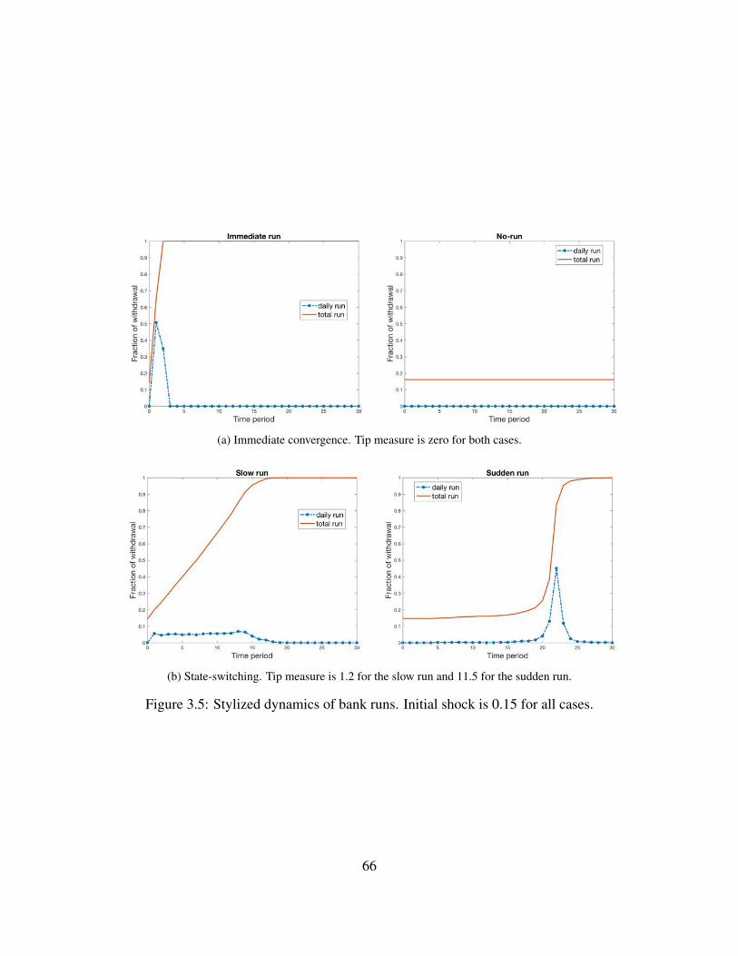
(a) Immediate convergence. Tip measure is zero for both cases.
(b) State-switching. Tip measure is 1.2 for the slow run and 11.5 for the sudden run.
Figure 3.5: Stylized dynamics of bank runs. Initial shock is 0.15 for all cases.
66

all depositors either withdraw or wait, depicted in Figure 3.5(a). The intuition follows from theproperties of thresholds. When liquidity is low, agents are very sensitive to any small amountof noises or fraction of withdrew neighbors. It takes only one or a few periods for all agents towithdraw. The reasoning is similar for high liquidity. To some extent, these instantaneous outcomesare related to symmetric equilibria in existing literature. Agents synchronize their action as if theymove simultaneously.
Second, state-switching occurs when withdrawals are made sequentially. There are two distinctstate-switching patterns: slow transition or sudden tip, depicted in Figure 3.5(b). Slow runs happenwhen withdrawals build up smoothly over time. In this case, daily withdrawals are visibly positiveand remain stable in a large time window. By contrast, sudden runs occurs in an abrupt manner.Daily withdrawals stay close to zero and suddenly jump to the maximum level. Switching patternis driven by the interplay between local and global mechanisms. Local interactions favor smoothtransition while global interactions facilitate sudden tip. More explanations will be provided insubsequent sections.
To distinguish these scenarios, survival time and tip measure are used. Survival time is close tozero for immediate run, while maximum for no-run. By convention, tip measure is zero for thesetrajectories. By contrast, switching trajectories have intermediate survival times with positive tipmeasures. Slow run has very low tip measure, the more sudden the run is, the higher its tip measure.
To summary, the stylized dynamics complement findings of the mean-field analysis, showinghow dynamic bank runs occur in different ways. In some cases, they span over a large time window.In other cases, they occur suddenly without any visible sign. The following sections investigate theeffects of the main parameters on the occurrence and characteristics of bank runs.
4.3 Liquidity vs. shockThe baseline model is studied in this section to focus on the interplay between liquidity reserve
(L) and initial shock (r0). Herding is fixed at h = 0.5. The main findings are presented in Figure3.6.
First, by survival time, panel 3.6(a) shows three distinct regions. Closest to the 45 degrees line,the deep blue region corresponds to the immediate failure zone, in which runs occurs instantly, suchthat survival time is close to 0. Conversely, the deep red region corresponds to the no-run zone,in which the bank always survives to the last period. This region is occupied mostly by no-runtrajectories. Finally, the region with mixing colors from light blue to light red corresponds to theswitching zone, in which survival time follows a positive and rather smooth evolution with relativeliquidity. These 3 regions confirm the previous findings, showing that dynamic bank runs occurswhen liquidity level is moderate compared to shock.
Second, pannel 3.6(b) identifies a very abrupt transition of bank failure, similar to a phase tran-sition. The outcomes are very stable for a wide range of parameters, then abruptly switches toanother state. Furthermore, a closer look at the frontier shows a very narrow subregion, character-ized by Pr(default) 2 (0,1). This subregion can be defined as the indeterminacy corridor, whereswitching trajectories occur randomly. The bank fails when switching occurs, otherwise no-runtrajectories take place and the bank survives.
67

Figure 3.6: The dynamics of bank runs, baseline model h = 0.5. Higher temperature color repre-sents higher value for the variable of interest.
68

The indeterminacy corridor might be explained by stochastic elements in the model. There are3 random factors: thresholds, signals and relative positions of runners. In general, the law of largenumbers stabilizes the outcomes, which are determined by whether liquidity or shock dominatesthe other. But when the two opposing forces are in balance, the system becomes sensitive to smallevents. The course of a trajectory can be altered by successive events that boost the number ofwithdrawals, such as: agents with low thresholds draw high signals in an ordering manner, runnersare clustered together within an optimal distance that increases contact with waiting agents andfacilitates local activation. To some extent, this finding is similar to the indeterminacy zone docu-mented in Arifovic et al. (2013), in which the experimental economy randomly switches betweenno-run and run equilibria for the same parameters. While their setting is different from this model,one common feature of the two findings is the path dependence property of bank runs trajectories.
Third, pannel 3.6(c) show the colored region in which tip measure is positive. This region is anapproximation for the switching zone, allowing the distinction between sudden runs and slow runs.Sudden run occurs for low liquidity levels, because the average threshold is low. A moderate jumpin total withdrawal is enough to make a large fraction of depositors withdraw in the subsequentperiod. For high liquidity level, the argument is simply reversed. Tip measure is highest around thetransition frontier, particularly within the indeterminacy corridor because of random switching.
Finally, the fitted curve in pannel 3.6(d) shows that the abruptness of runs is non-monotonicwith respect to liquidity buffers (L�r0). Switching trajectories become closer to immediate run forhigher shocks or lower liquidity levels, vice-versa for no-run. Combined with the phase transitionfrontier, this result implies that banks need to hold liquidity above a critical level to avoid panicruns. Otherwise, the surplus of liquidity makes runs delayed but more abrupt.
Overall, these results are aligned with previous findings and provide a general view on thedynamics of bank runs. Clearly low liquidity leads to immediate run, while clearly high liquidityleads to no run. For moderate liquidity, there are two distinct patterns: progressive withdrawals orsudden massive run.
4.4 HerdingThis section investigates the effects of herding on the dynamics and the occurrence of bank
runs. When the herding factor (h) decreases, individual decision is inclined toward private signalsthat are related to the available liquidity of the bank. On the contrary, when h increases, agentswill progressively disregard their own information and put more weight on the observed actions oftheir neighbors. Variation of the herding factor will alter the micro behaviors and have impact onthe aggregate dynamics. The main results are presented in Figure 3.7, the stacked heat maps showregions where tip measure is positive.
First, there is a very clear trend regarding the colors: runs become less abrupt as herding in-creases. This can be explained by the range of feedback mechanisms. When herding is strong, localinteractions build up the panic similarly to the spread of contagious diseases. Depositors are morelikely to be infected through direct contact with withdrew neighbors. Large clusters of runnersdevelop progressively and infect depositors who reside close to the boundaries of those clusters. Inconsequence, the panic takes time to spread out. By contrast, for weak herding, global mechanism
69

Figure 3.7: Effect of herding on tip measure. High temperature colors represent high values of tipmeasure.
70

Figure 3.8: Effects of herding on averaged probability of default. The shock (r0) is decomposedinto 5 quintiles. Each line represents the averaged probability of default for one specific quintile ofshock.
make signals diffuse “over the air” and bypass the localized network structure. Total withdrawalaccumulates slowly but it eventually reaches a critical mass, such that the chance to receive signalshigher than the average threshold is significant. Then, global interaction creates a generalized panicinstantly.
Second, runs are more frequent with strong herding. From bottom to top layers, the no-runregion shrinks (upper left triangle). Furthermore, the switching region expands on the left (low r0)and becomes flatten on the right (high r0). This change in aggregate behavior shows that the systemdoes not respond monotonically to different shock regimes, as herding increases.
To further investigate this effect, Figure 3.8 decomposes the distribution of shocks into 5 quin-tiles. There are 2 distinct macro behaviors with regard to shocks of different sizes. For the firstquintile of shocks i.e. r0 2 (0.01,0.2), the average probability of default increases with h. On thecontrary, for the third and fourth quintiles, the tendency is clearly reversed. This observation showsthat the bank becomes more fragile to small shocks and more robust to large shocks as herdingincreases.
These results can be explained as follows. Except for extreme values of h, the liquidity shockhas two initial impacts. First, agents surrounded by initial runners are likely to withdraw by localinteractions. Second, if the shock is not too small, it will generate enough noises that make otherrandom agents withdraw. The combined impact sets the initial condition for the cascading process.
For small shock, the initial withdrawals generate low signals on average. When herding isweak, small shocks can hardly make random agents withdraw by the global mechanism. However,when herding increases, small number of initial runners can trigger their neighbors to withdrawwith certainty. The global mechanism is weak in the beginning, but the local mechanism fills in to
71

build up cumulative withdrawal. In consequence, particularly for small shocks, increasing herdingfavors the occurrence of runs, making the bank more fragile.
For large shocks, the initial withdrawals generate high signals on average. If liquidity is low, thebank defaults immediately, only high liquidity levels are relevant to the discussion. When herdingis weak, random agents have high probability to withdraw regardless of their distance. However,when herding is strong, only agents located around initial runners will withdraw. Moreover, forlarge shocks, initial runners are more likely to form large clusters, their total contact with theremaining agents is further reduced. In consequence, increasing herding will reduce the earlyimpact of large shocks. Combined with the loss in speed due to herding, the reduction in earlyactivation makes large shocks less dangerous for banks, conditional on having high liquidity.
Overall, herding generates a tension between activation and speed, such that increase herdingmake runs more frequent but less abrupt. Strong herding favors early activation, but the cascade isslow because local interaction has limited range. By contrast, weak herding facilitates tipping. It ismore difficult for runs to start out, however, at some critical level, global interaction causes a panicinstantly. Depending on other parameters, these two opposing effects of herding may result in ahigher or lower probability of default.
4.5 Diversity: noises & thresholdsAs shown in the mean-field analysis, to have switching dynamics, it is necessary that agents
have different inputs to their decision-making process. To some extent, the differences acrossagents can be defined as diversity, with respect to information and type. In this model, g capturesthe variations of private signals and sq captures the differences in types that results in variations ofthresholds. This section will show how these two parameters affect dynamic bank runs.
Rt�1 t̄Pr(R̃it > ti)
R̃it ⇠ N (Rt�1,gRt�1) ti
Figure 3.9: Signals vs. thresholds. When diversity increases, the distributions have fatter tails.
72

Before getting into the results, it is important to show how the distributions of signals andthresholds shape the trajectories of runs. The effect of g is stronger with low values of h, as moreweight is put on private signals. To derive some insights, let consider the extreme case in whichh = 0, depicted in Figure 3.9. The probability to withdraw is the joint probability to draw highsignals and low thresholds. The distribution of thresholds is fixed while the distribution of signalsis endogenous and evolves over time. When total withdrawal increases, the distribution of signalsshifts to the right and get larger tails, proportional to g . The probability to withdraw determines themagnitude of the shift and how fat the tails become in the next period. This mechanism is similarto the mean-field case while allowing us to visualize the effect of diversity.
First, when diversity is low, the two distributions concentrate around their means, the proba-bility to withdraw is likely to be very small or even zero in early periods. On the contrary, morediversity makes fatter tails, such that the probability to withdraw is likely to be high. Hence, otherthings being equal, high levels of diversity will trigger more activation.
Second, as the distribution of signals evolves, diversity plays an important role in the abruptnessof runs. The key element is the expansion of the joint area. With low diversity, early fractions ofwithdrawals will be very small, as the two distributions have very thin tails. However, if total with-drawal keeps building up, the two distributions come progressively closer together. The overlappedarea suddenly gets very large around the means. This is the surprise effect: the jump in probabilityto withdraw produces a massive fraction of run compared to previous periods. Therefore, runs willbe delayed and abrupt if they occur in low diversity environment. On the contrary, high diversitywill make the joint area grow faster in a more stable way from the beginning.
Figure 3.10 shows the discussed results. Accordingly, increases in either g or sq (left panels)result in a higher average default rate. Furthermore, averaged tip measures decreases with respectto both parameters (right panels). The average tip measure decreases because runs are faster, bycontrast with the effect of herding. It may seem counterintuitive, but abruptness requires slow earlyaccumulation of withdrawals. High diversity accelerates the speed of accumulation, raising theinitial slope of switching trajectories, making runs more apparent but less abrupt. Thus, increasediversity makes runs occur more frequently and faster, strictly increasing the probability of default.
The idea that more diversity increases vulnerability may appear counterintuitive. It is helpfulto think in probabilistic dispersion. More diversity implies that there is a high chance that somedepositors are extremely “impatient” compared to others. There is also a high chance that some de-positors have very bad opinions about the robustness of the bank, compared to the average opinion.Together, these factors are more likely to trigger early withdrawals. The same process can applysequentially, making the panic cascade over the population. On the contrary, when depositors aresymmetric, they behave like one representative agent. There is strength in unity, because it is hardto make some depositors withdraw before others. When necessary conditions are met, depositorsare likely to withdraw simultaneously. Although using a different setting, the financial cascademodel of Iori et al. (2006) has a similar finding, in which heterogeneity among agents increases thefragility of the system.
The result on heterogeneity of this model might provide alternative explanation to a recentfinding in Arifovic et al. (2018). In their experiment, subjects play a repeated version of the si-multaneous game and have many decisions to make over time. They found that larger groups of
73
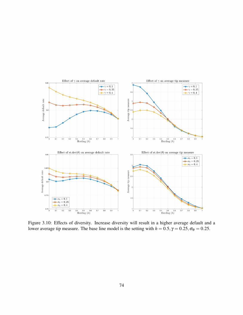
Figure 3.10: Effects of diversity. Increase diversity will result in a higher average default and alower average tip measure. The base line model is the setting with h = 0.5,g = 0.25,sq = 0.25.
74

subjects generate more bank runs compared to smaller groups, conditional on moderate liquidity(high early payoffs). To some extent, larger groups might imply larger intervals for the sensitivityto withdraw. For example, there is a higher chance to have subjects with extreme loss aversion.There are two consequences of high dispersion of sensitivity in large groups. First, the perceivedriskiness of the “wait” option might increase for any depositor, when they believe that some otherdepositors (even a small number) will withdraw with certainty. Second, when subjects make manydecisions over time and they know the total withdrawals in the past, there is a potential cascadeprocess similar to this model. As discussed previously, distribution of sensitivity with fatter tailsfacilitate activation of cascades. When depositors with extreme sensitivity withdraw in an earlyround, other highly sensitive depositors will follow in subsequent rounds. Over time, the averagedepositors are caught up in the cascade, when they learn that a large fraction of depositors withdrewin the last round.
4.6 Herding vs. diversityTo complete the picture, this section investigates the interaction between diversity and herding.
At a first glance, diversity and herding have the same qualitative effects: they both facilitate ac-tivation and reduce abruptness of runs. However, there is a main difference: the speed of runs isincreased with high diversity while reduced with high herding. Runs are less abrupt in both casesby design of the tipping measure.
Figure 3.10 shows the interplay between diversity and herding. It appears that strong herdingreduce the impacts of diversity, such that all the curves converge when h increases. By design, itis obvious that the effects of noises are washed out for high values of h. But why it is also thecase for thresholds? The answer comes from the network, precisely the small number of directneighbors. The idea can be illustrated with an extreme case in which h = 1. When local interactionis the only active force, each withdrawing neighbor has very large impact on individual decision.The variance in thresholds among waiting agents makes little difference when these agents aresurrounded by many withdrew neighbors. Unless the variance of thresholds is unusually large,such that the population is polarized: one group has very low thresholds and the other group hasvery high thresholds. In such case, the latter group will form clusters of resistance, like islands in asea of runners.
Furthermore, different levels of diversity can counter or enhance the effects of herding on bankfailure. Low diversity implies weak global mechanism, leaving the two opposing effects of herd-ing compete with each other. This combination generates non-monotonic effects when herdingincreases (lowest curves in the left panels). By contrast, high diversity brings in additional boostfor activation and speed. This boost is maximal when herding is low, but it fades out quickly whenherding increases. Thus, in high diversity environment, the effect of herding is quasi-monotonicrather than non-monotonic as in low diversity environment.
75

4.7 On network topologyAs discussed in previous sections, the network plays a significant role in channeling herding
behavior. The network acts as a platform on which herding operates. The topology of the networkand the parameter h go hand in hand to determine the extent of local interactions. However, thispaper focuses more on herding. There are many different network topologies with a wide range ofcharacteristics, a complete network analysis is beyond the scope of this paper. Some comparativestatics for different topologies can be found in the appendix. The results remain qualitatively robustto changes in network topology. This section provides some reflections on the network dimensionof the model.
First, observations are essential for herding. A reasonable assumption is that monitoring theactions of many agents at the same time is costly. Furthermore, it is also difficult to observe agentsthat are far way. These limits are not applied only to spatial dimension, but also to social andsectorial dimension, if depositors are firms or financial institutions. Therefore, to capture the effectof herding, the network should be localized. Furthermore, this type of topology is also consistentwith empirical findings (Iyer and Puri (2012); Atmaca et al. (2017)), in which only close neighborsor family members have significant effects on depositors’ decision.
Second, the effect of the topology become dominant only when herding is strong. Then, thedecision-making process approach naïve learning, where agents strongly incline to imitate theirneighbors. However, actions are costly in bank run, unlike other social phenomena such as fashionor opinion diffusion. Thus, very strong herding appears to be unrealistic for this model. The effectsof the network will be more influential when herding is endogenized, such that agents determinetheir tendency to herd base on the structure of links and their local position. This will be a futureextension of the model.
5 Discussion and conclusionThis paper has studied bank runs in a dynamic and behavioral setting. Panic bank runs arise as
cascades of decisions by both strategic complementarity and herding.The model is able to characterize the frequency, speed and abruptness of runs. Depending on the
parameters, there are three distinct patterns: immediate run, no-run and switching. For low, or highliquidity reserve respectively, all depositors either withdraw immediately, or don’t withdraw at all.For moderate liquidity, there are two patterns of bank runs: slow runs with sequential withdrawalsbuild up over time or sudden runs with massive withdrawals occur abruptly. Increase herdinggenerates a tension between activation and speed, such that runs are more frequent but also slower tospread out. Because of this tension, the overall effect of herding on bank failure is non-monotonic.By contrast, increase diversity facilitates both activation and speed, such that the probability ofbank failure is strictly increasing.
From a policy perspective, banks are currently required to hold at least 1% of certain liabili-ties, mainly customer deposits, as liquidity reserve. The liquidity requirement has a maintenancewindow of 2 weeks in the US and 6 weeks in the EU. This paper suggests several implications forbanks and policies makers.
76

First, it is important to actively monitor day-by-day withdrawals and adjust dynamically liquidityreserve, in addition to the minimum reserve requirements. The reason is that sequential withdrawalsare path-dependent, a small change in early withdrawals can have large impact on the trajectory ofruns. Therefore, it might be useful to develop a quantitative framework that is able to detect run-sensitive patterns of withdrawals, to devise interventions that dissolve or at least dampen potentialpanics in the early stage.Second, there might exist a trade off between stability and uncertainty. Increase liquidity holdingand restrain herd behavior can reduce the probability of runs, but also make potential runs moreunpredictable. Furthermore, banks may face double layers of uncertainty on whether a run mightoccur (random switching), but also when it could occur (sudden tip) if it is on the way. Any measureaiming at increasing the robustness of banks should also be followed by efforts to reduce uncer-tainty in forecasting sudden large withdrawals. One direct measure is to supervise factors that affectthe behavior of depositors such as social networks, tendency to herd and degree of heterogeneity.This paper showed that these specific factors play an important role in generating bank runs.
It is worth stressing that the present model is simple in some aspects. It serves as a first steptoward building a dynamic framework for panic events. There are several limitations that can beaddressed.The first limit is the exogenous nature of important elements, such as the herding factor and thestatic information network. Furthermore, depositors stick with simple decision rules and do notchange their behaviors during the crisis. To make the model more realistic, one can use a so-phisticated decision-making by allowing several features: endogenous herding with respect to thenetwork and withdrawals; memory with weighted averaged signals; dynamic evolution of network;exchange of information among connected agents. These features will allow the model to focusmore on the individual aspect, such as learning and social interactions.The second limit is the absence of reactions from the bank. In practice, banks do not sit still andwait for their liquidity reserves to be depleted. One can introduce an interbank market such thatbanks can borrow liquidity to face withdrawals. This feature can be used to study the systemicaspect, such as market freeze and contagious bank runs. When a bank experiences withdrawals,depositors might panic and run preemptively from connected banks, creating a generalized bankingpanic. Furthermore, when banks fear that depositors might herd, they will be reluctant to lend toothers, creating a feedback cycle.
Overall, integrating dynamics and behavioral factors to models with strategic complementarityis an important step for future research, at both micro and aggregate level.
Appendix
A. Network topologiesThe network used in the model is a two-dimension grid. This section introduces 4 additional
structures: random network, small-world, circle, regular-8. The random network and small-worldboth have average degree of 4, similar to the grid network used in the model. The average degree
77

Figure 3.11: Macro behaviors of networks
of the circle is 2 and 8 for the regular-8.Circle is a regular network with degree 2, in which every agent has one neighbor each side:
left and right. All agents form a closed ring. Regular-8 is similar to the circle, but each agent isconnected to 4 other agents on each side, instead of 1. Small-world starts out as a regular networkwith degree 4. Then, every link has a small probability to be rewired, such that some shortcuts aremade inside the ring. Random network starts out as a regular network with degree 4. Every linkhas a probability 1 to be rewired, such that all links are random.
Figure 10 compares the macro behavior for all networks, including the grid network as thebenchmark. Networks with the same average degree (grid, random, small-world) behave verysimilarly, regardless the structure. Higher average degree (regular-8) appears to decrease fragilitybut increase abruptness, vice-versa for low average degree. These observations suggest that theaverage number of neighbors might play an important role, otherwise the pattern of links has littleinfluence in this model.
78

ReferencesGeorge A Akerlof and Robert J Shiller. Animal spirits: How human psychology drives the economy,
and why it matters for global capitalism. Princeton university press, 2010.
Jasmina Arifovic, Janet Hua Jiang, and Yiping Xu. Experimental evidence of bank runs as purecoordination failures. Journal of Economic Dynamics and Control, 37(12):2446–2465, 2013.
Jasmina Arifovic, Cars Hommes, Anita Kopányi-Peuker, and Isabelle Salle. Are sunspots effectivein a big crowd? evidence from a large-scale bank run experiment. Working paper, 2018.
Sümeyra Atmaca, Koen Schoors, and Marijn Verschelde. Bank loyalty, social networks and crisis.Journal of Banking & Finance, 2017.
Yaron Azrieli and James Peck. A bank runs model with a continuum of types. Journal of EconomicTheory, 147(5):2040–2055, 2012.
Michelle Baddeley. Herding, social influence and economic decision-making: socio-psychologicaland neuroscientific analyses. Philosophical Transactions of the Royal Society of London B:Biological Sciences, 365(1538):281–290, 2010.
Abhijit V Banerjee. A simple model of herd behavior. The Quarterly Journal of Economics, 107(3):797–817, 1992.
Hans Carlsson and Eric Van Damme. Global games and equilibrium selection. Econometrica:Journal of the Econometric Society, pages 989–1018, 1993.
Carl Chiarella. The elements of a nonlinear theory of economic dynamics, volume 343. SpringerScience & Business Media, 2012.
Douglas W Diamond and Philip H Dybvig. Bank runs, deposit insurance, and liquidity. Journal ofpolitical economy, 91(3):401–419, 1983.
Rod Garratt and Todd Keister. Bank runs as coordination failures: An experimental study. Journalof Economic Behavior & Organization, 71(2):300–317, 2009.
Itay Goldstein and Ady Pauzner. Demand–deposit contracts and the probability of bank runs. theJournal of Finance, 60(3):1293–1327, 2005.
Mark Granovetter. Threshold models of collective behavior. American journal of sociology, 83(6):1420–1443, 1978.
Chao Gu. Herding and bank runs. Journal of Economic Theory, 146(1):163–188, 2011.
Giulia Iori, Saqib Jafarey, and Francisco G Padilla. Systemic risk on the interbank market. Journalof Economic Behavior & Organization, 61(4):525–542, 2006.
79

Rajkamal Iyer and Manju Puri. Understanding bank runs: The importance of depositor-bank rela-tionships and networks. American Economic Review, 102(4):1414–45, 2012.
Rajkamal Iyer, Manju Puri, and Nicholas Ryan. A tale of two runs: Depositor responses to banksolvency risk. The Journal of Finance, 71(6):2687–2726, 2016.
Daniel Kahneman. Maps of bounded rationality: Psychology for behavioral economics. Americaneconomic review, 93(5):1449–1475, 2003.
Morgan Kelly and Cormac O Grada. Market contagion: Evidence from the panics of 1854 and1857. American Economic Review, 90(5):1110–1124, 2000.
Hubert Janos Kiss, Ismael Rodriguez-Lara, and Alfonso Rosa-García. On the effects of depositinsurance and observability on bank runs: an experimental study. Journal of Money, Credit andBanking, 44(8):1651–1665, 2012.
Hubert Janos Kiss, Ismael Rodriguez-Lara, and Alfonso Rosa-García. Do social networks preventor promote bank runs? Journal of Economic Behavior & Organization, 101:87–99, 2014.
Carl-Johan Lindgren, Gillian G Garcia, and Matthew I Saal. Bank soundness and macroeconomicpolicy. International Monetary Fund, 1996.
John H Miller and Scott E Page. The standing ovation problem. Complexity, 9(5):8–16, 2004.
Stephen Morris and Hyun Song Shin. Global games: Theory and applications. 2001.
Thomas C Schelling. Dynamic models of segregation. Journal of mathematical sociology, 1(2):143–186, 1971.
Andrew Schotter and Tanju Yorulmazer. On the dynamics and severity of bank runs: An experi-mental study. Journal of Financial Intermediation, 18(2):217–241, 2009.
Duncan J Watts. A simple model of global cascades on random networks. Proceedings of theNational Academy of Sciences, 99(9):5766–5771, 2002.
Duncan J Watts and Peter Dodds. Threshold models of social influence. The Oxford handbook ofanalytical sociology, pages 475–497, 2009.
80