finding an appropriate equation to measure similarity … · 2017-08-25 · finding an appropriate...

METHODOLOGY ARTICLE Open Access

Finding an appropriate equation tomeasure similarity between binary vectors:case studies on Indonesian and Japaneseherbal medicinesSony Hartono Wijaya1,2, Farit Mochamad Afendi3, Irmanida Batubara4, Latifah K. Darusman4, Md Altaf-Ul-Amin1

and Shigehiko Kanaya1*

Abstract

Background: The binary similarity and dissimilarity measures have critical roles in the processing of data consistingof binary vectors in various fields including bioinformatics and chemometrics. These metrics express the similarityand dissimilarity values between two binary vectors in terms of the positive matches, absence mismatches ornegative matches. To our knowledge, there is no published work presenting a systematic way of finding anappropriate equation to measure binary similarity that performs well for certain data type or application. A propermethod to select a suitable binary similarity or dissimilarity measure is needed to obtain better classification results.

Results: In this study, we proposed a novel approach to select binary similarity and dissimilarity measures. Wecollected 79 binary similarity and dissimilarity equations by extensive literature search and implemented thoseequations as an R package called bmeasures. We applied these metrics to quantify the similarity and dissimilaritybetween herbal medicine formulas belonging to the Indonesian Jamu and Japanese Kampo separately. We assessedthe capability of binary equations to classify herbal medicine pairs into match and mismatch efficacies based on theirsimilarity or dissimilarity coefficients using the Receiver Operating Characteristic (ROC) curve analysis. According to thearea under the ROC curve results, we found Indonesian Jamu and Japanese Kampo datasets obtained different rankingof binary similarity and dissimilarity measures. Out of all the equations, the Forbes-2 similarity and the Variantof Correlation similarity measures are recommended for studying the relationship between Jamu formulas andKampo formulas, respectively.

Conclusions: The selection of binary similarity and dissimilarity measures for multivariate analysis is datadependent. The proposed method can be used to find the most suitable binary similarity and dissimilarityequation wisely for a particular data. Our finding suggests that all four types of matching quantities in theOperational Taxonomic Unit (OTU) table are important to calculate the similarity and dissimilarity coefficientsbetween herbal medicine formulas. Also, the binary similarity and dissimilarity measures that include the negativematch quantity d achieve better capability to separate herbal medicine pairs compared to equations that exclude d.

Keywords: Binary data, Similarity measures, Distance metric, Jamu, Kampo, ROC curve, Hierarchical clustering

* Correspondence: [email protected] School of Information Science, Nara Institute of Science andTechnology, 8916-5 Takayama, Ikoma, Nara 630-0192, JapanFull list of author information is available at the end of the article

© The Author(s). 2016 Open Access This article is distributed under the terms of the Creative Commons Attribution 4.0International License (http://creativecommons.org/licenses/by/4.0/), which permits unrestricted use, distribution, andreproduction in any medium, provided you give appropriate credit to the original author(s) and the source, provide a link tothe Creative Commons license, and indicate if changes were made. The Creative Commons Public Domain Dedication waiver(http://creativecommons.org/publicdomain/zero/1.0/) applies to the data made available in this article, unless otherwise stated.

Wijaya et al. BMC Bioinformatics (2016) 17:520 DOI 10.1186/s12859-016-1392-z

http://crossmark.crossref.org/dialog/?doi=10.1186/s12859-016-1392-z&domain=pdf

mailto:[email protected]

http://creativecommons.org/licenses/by/4.0/

http://creativecommons.org/publicdomain/zero/1.0/

BackgroundBinary features have been commonly used to represent agreat variety of data [1–3], expressing the binary statusof samples as presence/absence, yes/no, or true/false. Ithas many applications in the bioinformatics, chemo-metrics, and medical fields [4–19], as well as in patternrecognition, information retrieval, statistical analysis,and data mining [20, 21]. The choice of an appropriatecoefficient of similarity or dissimilarity is necessary toevaluate multivariate data represented by binary featurevectors because different similarity measures may yieldconflicting results [22]. Choi et al. [23] collected binarysimilarity and dissimilarity measures used over the lastcentury and revealed their correlation through thehierarchical clustering technique. They also classifiedequations into two groups based on inclusion and exclu-sion of negative matches. Consonni & Todeschini [1]proposed five new similarity coefficients and comparedthose coefficients with some well-known similarity coef-ficients. Three of the five similarity coefficients are lesscorrelated with the other common similarity coefficientsand need an investigation to understand their potential.Meanwhile, Todeschini et al. [24] reported an analysis of44 different similarity coefficients for computing thesimilarities between binary fingerprints by using simpledescriptive statistics, correlation analysis, multidimen-sional scaling Hasse diagrams, and their proposedmethod ‘atemporal target diffusion model’.Nowadays, the utilization of herbal medicines, i.e.

Indonesian Jamu, Japanese Kampo, traditional Chinesemedicine (TCM), and so on [25], are becoming popularfor disease treatment and maintaining good health. Incase of Indonesian Jamu, each Jamu medicine is pre-pared from a single plant or a mixture of several plantsas its ingredients. The National Agency of Drug andFood Control (NA-DFC) of Indonesia supervises theproduction of Jamu medicines before its release for pub-lic use. Up to 2014, there were 1247 Jamu factories inIndonesia [26]. They have concocted a lot of Jamu for-mulas with various efficacies. Consequently, the studiesof Jamu formulas have become an interesting researchtopic in the last few years. It may be related to the prob-lems of the Jamu philosophy, systematization of Jamu, orphytochemistry. In the Jamu studies, the relationshipsbetween plants, Jamu, and efficacies lead to determineimportant plants for every disease class using globaland local approaches [4, 5, 27]. In addition, Kampoformulas are traditional medicines from Japan. Theseare generally prepared by combination of crudedrugs. In total, 294 Kampo formulas are listed in theJapanese Pharmacopoeia of 2012 and it can be usedfor self-medication [28]. Currently, many researchershave done Kampo studies to unveil the complexsystems of Kampo medication and to reveal the

scientific aspect of its relevance to modern health-care. In Jamu and Kampo studies, herbal medicineformula and plant/crude drug relations are repre-sented as binary feature vectors, denoting whether aparticular plant is used or not as an ingredient.The relationships between Jamu formulas, as well as

Kampo formulas and other herbal medicines, are notonly reflected by the efficacy similarity but also by theingredient similarity. One Jamu formula can be sug-gested as an alternative to the other one if they haverelatively similar ingredients. For mathematical analysis,each Jamu formula is represented as a binary vectorusing 1 to indicate the presence of a plant and 0 other-wise. However, each Jamu formula usually uses a fewplants. Thus, most of the Jamu vectors contain a few 1 sand many 0 s. Consequently, the number of plants thatare used simultaneously in Jamu pairs is much smallerthan the number of plants that are not used simultan-eously as Jamu ingredients. Therefore, in order to findrelatively similar Jamu formulas, the high number ofnegative matches might influence the calculation of bin-ary similarity or dissimilarity between Jamu pairs. Onthe other hand, there is no guarantee that negative co-occurrence between two entities is identical [29]. Hence,it is necessary to examine the binary similarity and dis-similarity coefficients of Jamu formulas to determine theappropriate measurement for finding a suitable mixingalternative of a target crude drug.Currently, there are several methods to measure the

quality of classifiers [30, 31] such as the Receiver Oper-ating Characteristic (ROC) curves [32, 33], Precision-Recall (PR) curves [33, 34], Cohen’s Kappa scores [35,36], and so on. An ROC curve is a very powerful tool formeasuring classifiers’ performance in many fields, espe-cially in the machine learning and binary-class problems[37]. The purpose of ROC analysis is similar to that ofthe Cohen’s Kappa, which is mainly used for rankingclassifiers. The ROC curve conveys more informationthan Cohen’s Kappa in a sense that it can also visualizethe performance of a classifier by a curve instead ofgenerating just a scalar value. In this study, wepropose a method to select the most suitable simi-larity measures in the context of classification basedon False Positive Rates (FPRs) and True PositiveRates (TPRs) by using ROC curve analysis. We dis-cuss the step-by-step development of this method byapplying it to assess the similarity of herbal medi-cines in the context of their efficacies. Initially, wegathered 79 binary similarity and dissimilarity equa-tions. Some identical equations were eliminated in thepreliminary step. Subsequently, the capability of bin-ary measures to separate herbal medicine pairs intomatch and mismatch efficacy groups was assessed byusing the ROC analysis.

Wijaya et al. BMC Bioinformatics (2016) 17:520 of 19

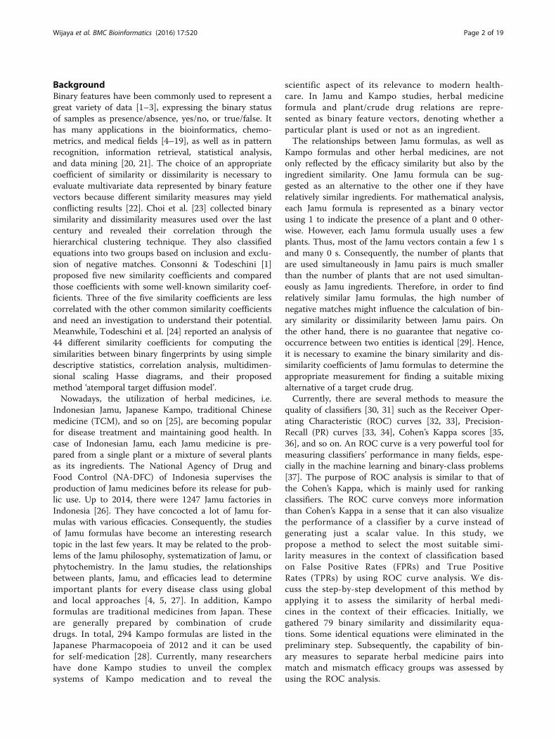
MethodsThe proposed method leads to the selection of a suitableequation such that when two herbal medicine formulasbelong to the same efficacy group, their ingredientsimilarity measured by the equation becomes higher inthe global context of a large set of formulas. Figure 1

illustrates data representation and also the procedure ofour experiment.

DatasetsWe used 3131 Jamu formulas collected from NA-DFCof Indonesia [4, 5, 27], which comprise of 465 plants.

a

b

c

Fig. 1 An illustration of the experimental flow. This figure also illustrates representation of plant, herbal medicine formulas and efficacy relationsas two-dimensional matrix. a Format of the input data representing Jamu-plant relations and the OTUs expression of a Jamu pair. b Reducing thecandidate equations. c The ROC analysis


Thus, Jamu vs. plant relations were then organized as a3131x465 matrix (Fig. 1a). Jamu formulas were repre-sented by binary vectors, which express the binary statusof plants as ingredients, 1 (presence) and 0 (absence).Each Jamu formula consists of 1 to 26 plants, with aver-age 4.904, standard deviation 2.969 and the set union ofall formulas consists of 465 plants. Each Jamu formulacorresponds to one or more efficacy/disease classes.Total 14 disease classes are used in this Jamu study, ofwhich 12 classes are from the National Center for Bio-technology Information (NCBI) [38]. The list of diseaseclasses are as follows: blood and lymph diseases (E1),cancers (E2), the digestive system (E3), female-specificdiseases (E4), the heart and blood vessels (E5), diseasesof the immune system (E6), male-specific diseases (E7),muscle and bone (E8), the nervous system (E9), nutri-tional and metabolic diseases (E10), respiratory diseases(E11), skin and connective tissue (E12), the urinary sys-tem (E13), and mental and behavioral disorders (E14).Corresponding to 3131 Jamu formulas, there can be(3,131x3,130)/2 = 4,900,015 Jamu pairs.For the purpose of comparison, we created four ran-

dom matrices as the same size as Jamu-plant relationsby randomly inserting 1 s and 0 s. In three of the ran-dom datasets, the numbers of 1 s are 1, 5 and 10% of465 plants (called as random 1%, random 5%, and ran-dom 10%). In the case of the other dataset, we randomlyinserted the equal number of 1 s in every row as it is inthe original Jamu formulas (called as random Jamu). Wealso applied our proposed method into Kampo dataset[28]. This dataset is presented as a two-dimensionalbinary matrix with rows and columns representingKampo formulas and crude drug ingredients, respect-ively. Kampo dataset is composed of 274 Kampo formu-las and each formula consists of 3 to 19 crude drugs,with average 8.923, standard deviation 3.885, and the setunion of all formulas consists of 227 crude drugs. Then,each Kampo formula is classified into deficiency or ex-cess class, according to Kampo-specific diagnosis of pa-tient’s constitution.

Flow of the experimentThe binary similarity (S) and dissimilarity (D) measurebetween a herbal medicine pair is expressed by the Op-erational Taxonomic Units (OTUs as shown in Fig. 1a)[39, 40]. Concretely, let two Jamu formulas be describedby two-row vectors Ji and Ji’, each comprised of M vari-ables with value 1 (presence) or 0 (absence). The fourquantities a, b, c, d in the OTUs table are defined as fol-lows: a is the number of features where the values forboth ji and ji’ are 1 (positive matches), b and c are thenumber of features where the value for ji is 0 and ji’ is 1and vice versa, respectively (absence mismatches), and dis the number of features where the values for both ji

and ji’ are 0 (negative matches). The sum of a and d rep-resents the total number of matches between ji and ji’,the sum of b and c represents the total number of mis-matches between ji and ji’. The total sum of the quan-tities in the OTUs table a + b + c + d is equal to M.We collected equations to measure similarity or

dissimilarity between binary vectors from literature[1, 3, 20, 21, 23, 24, 29, 40–62], listed as Eqs. 1-79in Table 1. The binary similarity and dissimilarityequations were represented by four quantities, i.e. a,b, c and d. We also implemented these 79 equationsas an R package, called bmeasures. The bmeasurespackage is available on Github and can be installedby invoking these commands: install.packages(“devtools”), library(“devtools”), install_github(“shwijaya/bmeasures”), library(“b-measures”). The installation of bmeasures package wastested on R release 3.2.4 and the devtools package ver.1.11.0. Initially, we measure the similarity and dissimilaritycoefficients between herbal medicine pairs by using 79equations. Then, the resulted similarity/dissimilarity coef-ficients are used for further analysis. Our experimentalprocedure can be divided into two major steps, which wediscuss in the following segments:Step 1. Reducing the candidate equationsThe binary similarity and dissimilarity equations were

evaluated to eliminate duplications. When two or moreequations can be transformed into the same form by al-gebraic manipulations, only one of them is kept for fur-ther analysis. We also removed equations from ouranalysis that produce infinite/NaN values or indetermin-ate forms while applying to measure similarity and dis-similarity using all datasets.Hierarchical clustering of the remaining equations was

then done with an aim to further narrow down the num-ber of candidate equations and to evaluate the closenessbetween equations. After we obtained the similarity/dis-similarity coefficients between herbal medicine pairs foreach equation, we clustered those equations based on itssimilarity/dissimilarity coefficients using Agglomerativehierarchical clustering with Centroid linkage (Fig. 1b)[50, 63–65]. The Euclidean distance (Eq. 80) was usedto measure the distance between two equations, kand l, that is:

dk;l ¼ffiffiffiffiffiffiffiffiffiffiffiffiffiffiffiffiffiffiffiffiffiffiffiffiffiffiffiffiffiffiffiffiffiffiffiffiffiffiffiffiffiffiffiffiffiffiffiffiffiffiffiffiffiffiffiffiffiffiffiffiffiffiffiffiffiffiXN−1

m¼1

XN

n¼mþ1smn kð Þ−smn lð Þð Þ2

rð80Þ

where smn(k) and smn(l) are the similarity/dissimilarityvalues between corresponding herbal medicine pairusing equations k and l respectively, N is the total num-ber of herbal medicine formulas, and dk,l is the distancebetween equation k and l. The cluster centroid is theaverage values of the variables for the observations (in


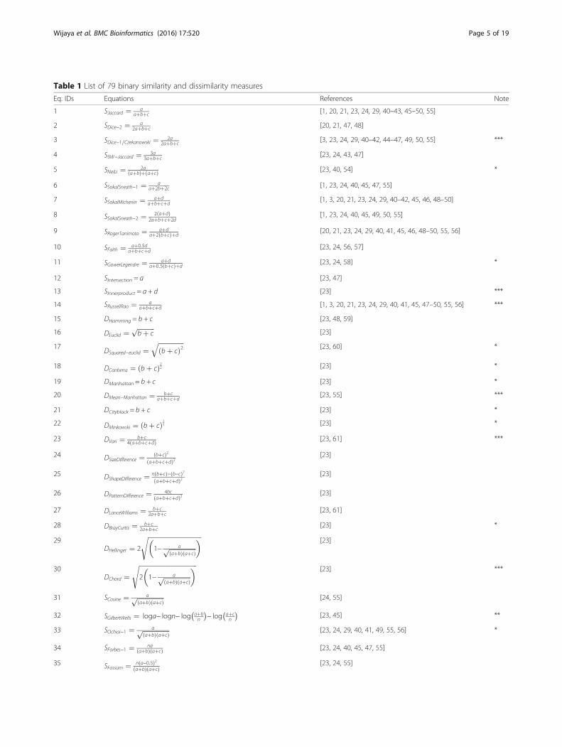
Table 1 List of 79 binary similarity and dissimilarity measures

Eq. IDs Equations References Note

1 SJaccard ¼ aaþbþc [1, 20, 21, 23, 24, 29, 40–43, 45–50, 55]

2 SDice−2 ¼ a2aþbþc [20, 21, 47, 48]

3 SDice−1=Czekanowski ¼ 2a2aþbþc

[3, 23, 24, 29, 40–42, 44–47, 49, 50, 55] ***

4 S3W−Jaccard ¼ 3a3aþbþc

[23, 24, 43, 47]

5 SNeiLi ¼ 2aaþbð Þþ aþcð Þ [23, 40, 54] *

6 SSokalSneath−1 ¼ aaþ2bþ2c [1, 23, 24, 40, 45, 47, 55]

7 SSokalMichener ¼ aþdaþbþcþd

[1, 3, 20, 21, 23, 24, 29, 40–42, 45, 46, 48–50]

8 SSokalSneath−2 ¼ 2 aþdð Þ2aþbþcþ2d

[1, 23, 24, 40, 45, 49, 50, 55]

9 SRogerTanimoto ¼ aþdaþ2 bþcð Þþd

[20, 21, 23, 24, 29, 40, 41, 45, 46, 48–50, 55, 56]

10 SFaith ¼ aþ0:5daþbþcþd

[23, 24, 56, 57]

11 SGowerLegendre ¼ aþdaþ0:5 bþcð Þþd

[23, 24, 58] *

12 SIntersection = a [23, 47]

13 SInnerproduct = a + d [23] ***

14 SRussellRao ¼ aaþbþcþd [1, 3, 20, 21, 23, 24, 29, 40, 41, 45, 47–50, 55, 56] ***

15 DHamming = b + c [23, 48, 59]

16 DEuclid ¼ffiffiffiffiffiffiffiffiffiffiffibþ c

p[23]

17DSquared−euclid ¼

ffiffiffiffiffiffiffiffiffiffiffiffiffiffiffiffibþ cð Þ2

q[23, 60] *

18 DCanberra ¼ bþ cð Þ22 [23] *

19 DManhattan = b + c [23] *

20 DMean−Manhattan ¼ bþcaþbþcþd

[23, 55] ***

21 DCityblock = b + c [23] *

22 DMinkowski ¼ bþ cð Þ11 [23] *

23 DVari ¼ bþc4 aþbþcþdð Þ [23, 61] ***

24 DSizeDifference ¼ bþcð Þ2aþbþcþdð Þ2

[23]

25 DShapeDifference ¼ n bþcð Þ− b−cð Þ2aþbþcþdð Þ2

[23]

26 DPatternDifference ¼ 4bcaþbþcþdð Þ2 [23]

27 DLanceWilliams ¼ bþc2aþbþc

[23, 61]

28 DBrayCurtis ¼ bþc2aþbþc

[23] *

29DHellinger ¼ 2

ffiffiffiffiffiffiffiffiffiffiffiffiffiffiffiffiffiffiffiffiffiffiffiffiffiffiffiffiffiffiffiffiffiffi1− affiffiffiffiffiffiffiffiffiffiffiffiffiffiffiffiffi

aþbð Þ aþcð Þp

� �s[23]

30DChord ¼

ffiffiffiffiffiffiffiffiffiffiffiffiffiffiffiffiffiffiffiffiffiffiffiffiffiffiffiffiffiffiffiffiffiffiffiffiffi2 1− affiffiffiffiffiffiffiffiffiffiffiffiffiffiffiffiffi


� �s[23] ***

31 SCosine ¼ affiffiffiffiffiffiffiffiffiffiffiffiffiffiffiffiffiaþbð Þ aþcð Þ

p [24, 55]

32 SGilbertWells ¼ loga− logn− log aþbn

� �− log aþc

n

� �[23, 45] **

33 SOchiai−1 ¼ affiffiffiffiffiffiffiffiffiffiffiffiffiffiffiffiffiaþbð Þ aþcð Þ

p [23, 24, 29, 40, 41, 49, 55, 56] *

34 SForbes−1 ¼ naaþbð Þ aþcð Þ [23, 24, 40, 45, 47, 55]

35 SFossum ¼ n a−0:5ð Þ2aþbð Þ aþcð Þ

[23, 24, 55]


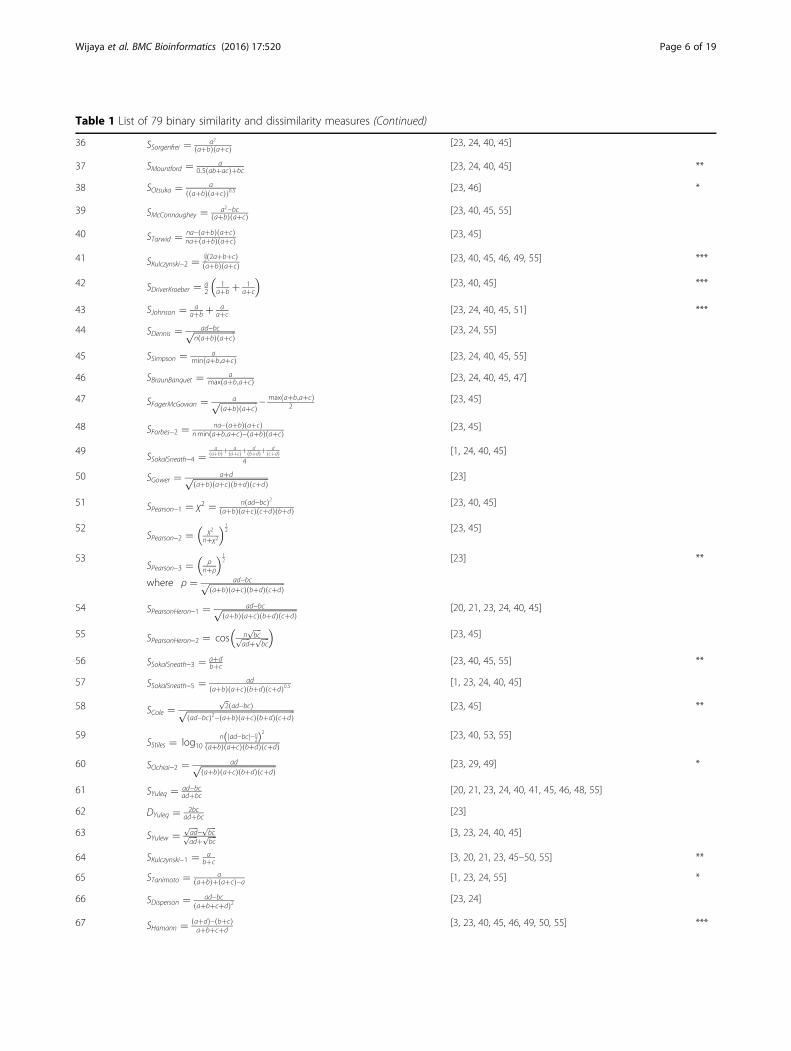
Table 1 List of 79 binary similarity and dissimilarity measures (Continued)

36 SSorgenfrei ¼ a2aþbð Þ aþcð Þ [23, 24, 40, 45]

37 SMountford ¼ a0:5 abþacð Þþbc [23, 24, 40, 45] **

38 SOtsuka ¼ aaþbð Þ aþcð Þð Þ0:5 [23, 46] *

39 SMcConnaughey ¼ a2−bcaþbð Þ aþcð Þ [23, 40, 45, 55]

40 STarwid ¼ na− aþbð Þ aþcð Þnaþ aþbð Þ aþcð Þ [23, 45]

41 SKulczynski−2 ¼a2 2aþbþcð Þaþbð Þ aþcð Þ

[23, 40, 45, 46, 49, 55] ***

42 SDriverKroeber ¼ a2

1aþb þ 1

aþc

� �[23, 40, 45] ***

43 SJohnson ¼ aaþb þ a

aþc [23, 24, 40, 45, 51] ***

44 SDennis ¼ ad−bcffiffiffiffiffiffiffiffiffiffiffiffiffiffiffiffiffiffiffin aþbð Þ aþcð Þ

p [23, 24, 55]

45 SSimpson ¼ amin aþb;aþcð Þ [23, 24, 40, 45, 55]

46 SBraunBanquet ¼ amax aþb;aþcð Þ [23, 24, 40, 45, 47]

47 SFagerMcGowan ¼ affiffiffiffiffiffiffiffiffiffiffiffiffiffiffiffiffiaþbð Þ aþcð Þ

p − max aþb;aþcð Þ2

[23, 45]

48 SForbes−2 ¼ na− aþbð Þ aþcð Þnmin aþb;aþcð Þ− aþbð Þ aþcð Þ [23, 45]

49SSokalSneath−4 ¼

aaþbð Þþ a

aþcð Þþ dbþdð Þþ d

cþdð Þ4

[1, 24, 40, 45]

50 SGower ¼ aþdffiffiffiffiffiffiffiffiffiffiffiffiffiffiffiffiffiffiffiffiffiffiffiffiffiffiffiffiffiffiffiffiffiffiaþbð Þ aþcð Þ bþdð Þ cþdð Þ

p [23]

51 SPearson−1 ¼ χ2 ¼ n ad−bcð Þ2aþbð Þ aþcð Þ cþdð Þ bþdð Þ

[23, 40, 45]

52SPearson−2 ¼ χ2

nþχ2

� �12 [23, 45]

53SPearson−3 ¼ ρ

nþρ

� �12

where ρ ¼ ad−bcffiffiffiffiffiffiffiffiffiffiffiffiffiffiffiffiffiffiffiffiffiffiffiffiffiffiffiffiffiffiffiffiffiffiaþbð Þ aþcð Þ bþdð Þ cþdð Þ

p

[23] **

54 SPearsonHeron−1 ¼ ad−bcffiffiffiffiffiffiffiffiffiffiffiffiffiffiffiffiffiffiffiffiffiffiffiffiffiffiffiffiffiffiffiffiffiffiaþbð Þ aþcð Þ bþdð Þ cþdð Þ

p [20, 21, 23, 24, 40, 45]

55 SPearsonHeron−2 ¼ cos πffiffiffiffibc

pffiffiffiffiad

p þ ffiffiffiffibc

p� �

[23, 45]

56 SSokalSneath−3 ¼ aþdbþc

[23, 40, 45, 55] **

57 SSokalSneath−5 ¼ adaþbð Þ aþcð Þ bþdð Þ cþdð Þ0:5 [1, 23, 24, 40, 45]

58 SCole ¼ffiffi2

pad−bcð Þffiffiffiffiffiffiffiffiffiffiffiffiffiffiffiffiffiffiffiffiffiffiffiffiffiffiffiffiffiffiffiffiffiffiffiffiffiffiffiffiffiffiffiffiffiffiffiffiffi

ad−bcð Þ2− aþbð Þ aþcð Þ bþdð Þ cþdð Þp [23, 45] **

59SStiles ¼ log10

n ad−bcj j−n2ð Þ2

aþbð Þ aþcð Þ bþdð Þ cþdð Þ[23, 40, 53, 55]

60 SOchiai−2 ¼ adffiffiffiffiffiffiffiffiffiffiffiffiffiffiffiffiffiffiffiffiffiffiffiffiffiffiffiffiffiffiffiffiffiffiaþbð Þ aþcð Þ bþdð Þ cþdð Þ

p [23, 29, 49] *

61 SYuleq ¼ ad−bcadþbc

[20, 21, 23, 24, 40, 41, 45, 46, 48, 55]

62 DYuleq ¼ 2bcadþbc

[23]

63 SYulew ¼ffiffiffiffiad

p−ffiffiffiffibc

pffiffiffiffiad

p þ ffiffiffiffibc

p [3, 23, 24, 40, 45]

64 SKulczynski−1 ¼ abþc [3, 20, 21, 23, 45–50, 55] **

65 STanimoto ¼ aaþbð Þþ aþcð Þ−a [1, 23, 24, 55] *

66 SDisperson ¼ ad−bcaþbþcþdð Þ2 [23, 24]

67 SHamann ¼ aþdð Þ− bþcð Þaþbþcþd

[3, 23, 40, 45, 46, 49, 50, 55] ***


the present case equations) in that cluster. Let XG;XH

denote group averages for clusters G and H. Then,the distance between cluster centroids is calculatedusing Eq. 81.

dcentroid G;Hð Þ ¼ XG

−XH

2 ð81Þ

where XG is the centroid of G by arithmetic mean XG ¼1nG

XnG

i¼1XGi [2, 65, 66]. We implemented the clustering

process using hclust function in R. At each step, thecluster centroid was calculated to represent a group ofequations in the clusters. Furthermore, two equations orclusters are merged for which the distance between thecentroids is the minimum until all equations are mergedinto one cluster.We performed the hierarchical clustering process

twice, first to reduce the candidate equations for whichthe distance between equations measured by Eq. 80 iszero or nearly zero and secondly to evaluate the com-bined characteristic of a group of equations. Mean cen-tering and unit variance scaling was applied to thesimilarity/dissimilarity coefficients before the clusteringprocess.Step 2. ROC Analysis of selected equationsThe effectiveness of similarity/dissimilarity measur-

ing capability of the selected equations was evaluatedby means of the ROC curve (Fig. 1c) [67, 68]. ForROC analysis, we divided all the herbal medicine

pairs into match and mismatch efficacy classes andused the corresponding distributions with respect tosimilarity scores to calculate FPRs and TPRs. TheROC curve was created by selecting a series ofthreshold to generate FPR and TPR. FPR is the pro-portion of false positive predictions out of all thefalse data and TPR is the proportion of true positivepredictions out of all the true data, defined byEq. 82 [67–69]:

FPR ¼ FP= FP þ TNð Þ TPR ¼ TP= TP þ FNð Þð82Þ

where true positive (TP) is the number of herbal medi-cine pairs correctly classified as positive, true negative(TN) is the number of pairs correctly classified as nega-tive, false positive (FP) is the number of pairs incorrectlyclassified as positive, and false negative (FN) is the num-ber of pairs incorrectly classified as negative. We definedand compared the performance of good equations byusing the minimum distance of the ROC curve to thetheoretical optimum point and by using the Area Underthe ROC Curve (AUC) analysis [70]. The minimum dis-tance between the ROC curve and the optimum pointwas measured as the Euclidean distance. The minimumdistance can also be computed by TP, TN, FP, and FNvalues corresponding to selected similarity thresholds iusing the following formulation:

Table 1 List of 79 binary similarity and dissimilarity measures (Continued)

68 SMichael ¼ 4 ad−bcð Þaþdð Þ2þ bþcð Þ2

[23, 24, 40, 45, 52]

69 SGoodmanKruskal ¼ σ−σ0

2n−σ0

whereσ ¼ max a; bð Þ þ max c; dð Þ þ max a; cð Þ þ max b; dð Þσ

0 ¼ max aþ c; bþ dð Þ þ max aþ b; c þ dð Þ

[23] **

70 SAnderberg ¼ σ−σ0

2n[23] **

71 SBaroni−UrbaniBuser−1 ¼ffiffiffiffiad

p þaffiffiffiffiad

p þaþbþc[23, 24, 40, 45, 55, 56, 62]


p þa− bþcð Þffiffiffiffiad

p þaþbþc[23, 24, 40, 45, 62] ***

73 SPeirce ¼ abþbcabþ2bcþcd

[23, 45] **

74 SEyraud ¼ n2 na− aþbð Þ aþcð Þð Þaþbð Þ aþcð Þ bþdð Þ cþdð Þ

[23]

75 STarantula ¼a

aþbð Þc

cþdð Þ¼ a cþdð Þ

c aþbð Þ.[23] **

76SAmple ¼

aaþbð Þc

cþdð Þ

¼ a cþdð Þ

c aþbð Þ . [23] **

77 SDerivedRusell−Rao ¼ log 1það Þlog 1þnð Þ. [1, 24]

78 SDerivedJaccard ¼ log 1það Þlog 1þaþbþcð Þ [1, 24]

79 SVarof Correlation ¼ log 1þadð Þ− log 1þbcð Þlog 1þn2=4ð Þ [1, 24]

S is similarity measure, D is dissimilarity measure, *means algebraically redundant, **means produce infinite/NaN coefficients or indeterminate forms, ***means groupedin the same cluster with zero or nearly to zero distance, n is a constant (n =M = a + b + c + d)


Min: dist

¼ mini ∈ thresholds

ffiffiffiffiffiffiffiffiffiffiffiffiffiffiffiffiffiffiffiffiffiffiffiffiffiffiffiffiffiffiffiffiffiffiffiffiffiffiffiffiffiffiffiffiffiffiffiffiffiffiffiffiffiffiffiffiffiffiffiffiffiffiffiffiffiffiffiffiffiffiffiffiffiffiffiffiffiffiffiffiffiffiffiffiffiffiffiffiFPi= TNi þ FPið Þð Þ2 þ FNi= TPi þ FNið Þð Þ2

qð83Þ

Results and discussionPreliminary verification of the equationsIn the preliminary step, we removed 12 equations de-noted by ‘*’ in Table 1 because each of them can be rec-ognized as identical to one or more other equations byonly algebraic manipulations such as linear transform-ation. From the seven groups of redundant equationsshown in Table 2, we included SJaccard, SDice-1/Czekanowski,SSokal&Sneath-2, DHamming, DLance&Williams, SCosine andSSokal&Sneath-5 in our analysis and therefore, we wereleft with 67 equations at this stage. Next, we clusteredthe 67 equations to reduce the number of equationsusing Jamu and Kampo datasets. During the clusteringprocess, we eliminated 11 equations indicated by ‘**’ inTable 1 that produced infinite/NaN values or indetermin-ate forms while applied to all datasets. Such conditionscan be reached when denominator of an equation be-comes equal to 0, i.e. the values of b and c in the Mount-ford and Peirce similarities (Eq. 37 and Eq. 73) are 0 if twoformulas use exactly the same ingredients.The clustering of 56 equations in the context of Jamu

data is shown in Fig. 2. The distances among equationsbelonging to individual clusters indicated as 1 to 7 inFig. 2 are equal or nearly equal to 0. In other words,those equations have similar characteristics whengenerating binary similarity/dissimilarity coefficients forJamu data. By using the clustering result, we reduced 11equations denoted by ‘***’ in Table 1 because they were

related to other equations in the same cluster e.g. weeliminated SBaroni-Urbani&Buser-2 (Eq. 72) because it issimilar to SBaroni-Urbani&Buser-1 (Eq. 71). A careful obser-vation of equations belonging to the same cluster in thegroup IDs 1 to 7 in Fig. 2 implies that one equation canbe transformed to another just by adding or multiplyingby constants (Table 3). For example, we can representSBaroni-Urbani&Buser-2 as [(2 x SBaroni-Urbani&Buser-1) – 1].The excluded equations based on the clustering processare as follows: SDice-1/Czekanowski (Eq. 3), SInnerproduct (Eq.13), SRussell&Rao (Eq. 14), DMean-Manhattan (Eq. 20), DVari

(Eq. 23), DChord (Eq. 30), SKulczynski-2 (Eq. 41), SDriver&Kroeber (Eq. 42), SJohnson (Eq. 43), SHamann (Eq. 67),and SBaroni-Urbani&Buser-2 (Eq. 72). In case of Kampodataset, the clustering results also identified the sameequations belong to the same cluster with zero ornearly to zero distance. Therefore, both datasets elimi-nated the same equations, indicated by ‘***” in Table 1,and also obtained the same number of selected equa-tions (45 binary similarity and dissimilarity measures)for further analysis. Hence, among the 79 binarysimilarity dissimilarity measures used over the last cen-tury, there are only 45 unique equations that producedifferent coefficients by capturing different informa-tion. Additionally, these binary measures satisfy thesymmetry property [71], i.e. in case of such equationsd(x, y) = d(y, x) or S(x, y) = S(y, x).We applied hierarchical clustering again to these 45

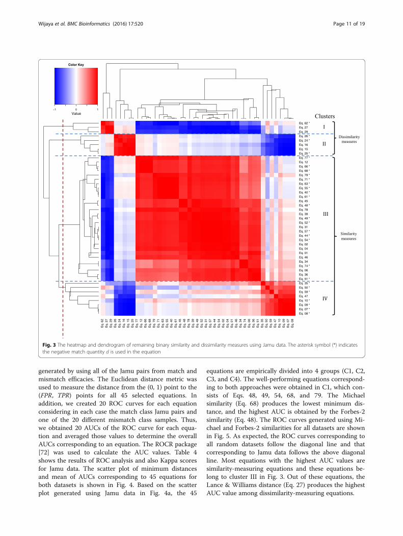
equations to give a better understanding of relationshipsbetween selected equations. In general, Jamu and Kampodata generated more or less the same heatmap. The re-sulted dendrogram together with the heatmap of Jamudata are shown in Fig. 3. We can roughly identify fourmain clusters (I, II, III, and IV). The hierarchical

Table 2 Groups of identical equations

Groups Eliminated Equations Selected Equations

1 SNeiLi ¼ 2aaþbð Þþ aþcð Þ (Eq.5) SDice−1=Czekanowski ¼ 2a

2aþbþc (Eq.3)

2 SGowerLegendre ¼ aþdaþ0:5 bþcð Þþd (Eq.11) SSokalSneath−2 ¼ 2 aþdð Þ

2aþbþcþ2d (Eq.8)

3DSquared−euclid ¼

ffiffiffiffiffiffiffiffiffiffiffiffiffiffiffiffibþ cð Þ2

q(Eq.17)

DHamming = b + c (Eq.15)

DCanberra ¼ bþ cð Þ22 (Eq.18)DManhattan = b + c (Eq.19)

DCityblock = b + c (Eq.21)

DMinkowski ¼ bþ cð Þ11 (Eq.22)4 DBrayCurtis ¼ bþc

2aþbþc (Eq.28) DLanceWilliams ¼ bþc2aþbþc (Eq.27)

5 SOchiai−1 ¼ affiffiffiffiffiffiffiffiffiffiffiffiffiffiffiffiffiaþbð Þ aþcð Þ

p (Eq.33) SCosine ¼ affiffiffiffiffiffiffiffiffiffiffiffiffiffiffiffiffiaþbð Þ aþcð Þ

p (Eq.31)

SOtsuka ¼ aaþbð Þ aþcð Þð Þ0:5 (Eq.38)

6 SOchiai−2 ¼ adffiffiffiffiffiffiffiffiffiffiffiffiffiffiffiffiffiffiffiffiffiffiffiffiffiffiffiffiffiffiffiffiffiffiaþbð Þ aþcð Þ bþdð Þ cþdð Þ

p (Eq.60) SSokalSneath−5 ¼ adaþbð Þ aþcð Þ bþdð Þ cþdð Þ0:5 (Eq.57)

7 STanimoto ¼ aaþbð Þþ aþcð Þ−a (Eq.65) SJaccard ¼ a

aþbþc (Eq.1)


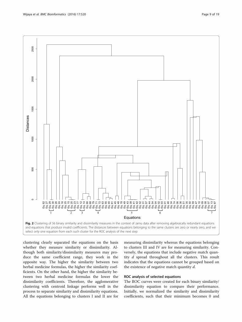
clustering clearly separated the equations on the basiswhether they measure similarity or dissimilarity. Al-though both similarity/dissimilarity measures may pro-duce the same coefficient range, they work in theopposite way. The higher the similarity between twoherbal medicine formulas, the higher the similarity coef-ficients. On the other hand, the higher the similarity be-tween two herbal medicine formulas the lower thedissimilarity coefficients. Therefore, the agglomerativeclustering with centroid linkage performs well in theprocess to separate similarity and dissimilarity equations.All the equations belonging to clusters I and II are for

measuring dissimilarity whereas the equations belongingto clusters III and IV are for measuring similarity. Con-versely, the equations that include negative match quan-tity d spread throughout all the clusters. This resultindicates that the equations cannot be grouped based onthe existence of negative match quantity d.

ROC analysis of selected equationsThe ROC curves were created for each binary similarity/dissimilarity equation to compare their performance.Initially, we normalized the similarity and dissimilaritycoefficients, such that their minimum becomes 0 and

Fig. 2 Clustering of 56 binary similarity and dissimilarity measures in the context of Jamu data after removing algebraically redundant equationsand equations that produce invalid coefficients. The distances between equations belonging to the same clusters are zero or nearly zero, and weselect only one equation from each such cluster for the ROC analysis of the next step


maximum becomes 1, before using them to create theROC curves. In the case of equations that measuredissimilarity, we transformed a normalized dissimi-larity coefficient D to a similarity coefficient S forthe sake of comparison by using the following equationS = 1 −D2 [40, 41].In the context of Jamu data, we started the ROC ana-

lysis of selected equations by classifying the Jamu pairsinto match and mismatch classes based on their effica-cies. A Jamu pair belongs to the match class if the effi-cacy of both the Jamu formulas of a pair is the same. Onthe other hand, a Jamu pair belongs to the mismatchclass if the efficacies of the formulas of a pair are differ-ent. The number of Jamu pairs in the match and mis-match classes are 646,728 and 4,253,287 respectively.Obviously, the number of Jamu pairs in the mismatchclass is much larger than that in the match class. Thisimbalance is a challenge in assessment of the capabilityof equations to separate Jamu pairs into match and mis-match classes. In order to handle this condition, we cre-ated 20 mismatch classes each equal to the size of thematch class by random sampling of the mismatch classJamu pairs according to bootstrap method [67]. Everyequation was then iteratively evaluated by using thosedatasets as mismatch class data.Our objective is to assess the capability of the

equations to separate the Jamu pairs into match andmismatch efficacy classes based on their similarity coeffi-cients using ROC analysis. In order to create an ROCcurve corresponding to an equation, we need the distri-butions of match class and mismatch class Jamu pairs

with respect to their similarity values calculated by theequation. We divided the range of the similarity coeffi-cient into 100 equal intervals, and the lower limit ofeach interval was considered as a threshold. Corre-sponding to every threshold, TP and FN were deter-mined from the distribution of match class and FP andTN were determined from the distribution of mismatchclass. In our case, TP and FP are the numbers of Jamupairs with the similarity value larger than or equal tothreshold, and FN and TN are the numbers of Jamupairs with the similarity value smaller than threshold.FPR and TPR were then calculated for every thresholdusing Eq. 82. We produced the ROC curve by plottingthe resulting FPR on the x-axis and TPR on the y-axis.In perfect or ideal classification, the ROC curve followsthe vertical line from (0,0) to (0,1) and then horizontalline up to (1,1). In the case of random data, the ROCcurve follows the diagonal line from (0,0) to (1,1). In thecase of real data, the ROC curve usually follows anabove diagonal line. The (0,1) is the optimum classifica-tion point where FPR is zero and TPR is one and hencethe (0,1) point will be referred to as ‘optimum point’.The performance of a classifier was assessed either bymeasuring the minimum distance from the optimumpoint to the curve or by measuring the AUC. In the caseof the minimum distance, the lower is the value of theminimum distance the better is the performance of theclassifier. In the case of the AUC, the bigger is the AUCvalue, the better is the performance of the classifier.In order to assess the effectiveness of an equation

using the minimum distance, the ROC curve was

Table 3 Transformation of an equation into another by adding or multiplying by constants (Group IDs correspond to clustersin Fig. 2)

Group IDs Eliminated Equations Selected Equationsa

1DChord ¼

ffiffiffiffiffiffiffiffiffiffiffiffiffiffiffiffiffiffiffiffiffiffiffiffiffiffiffiffiffiffiffiffiffiffiffiffiffi2 1− affiffiffiffiffiffiffiffiffiffiffiffiffiffiffiffiffi


� �s(Eq 30) ¼ 1ffiffi

2p 2

ffiffiffiffiffiffiffiffiffiffiffiffiffiffiffiffiffiffiffiffiffiffiffiffiffiffiffiffiffiffiffiffiffiffi1− affiffiffiffiffiffiffiffiffiffiffiffiffiffiffiffiffi


� �s¼ 1ffiffi

2p DHellinger (Eq.29)

2 DMean−Manhattan ¼ bþcaþbþcþd (Eq.20) ¼ 1

M bþ cð Þ ¼ 1MDHamming (Eq.15)

DVari ¼ bþc4 aþbþcþdð Þ (Eq.23) ¼ 1

4M bþ cð Þ ¼ 14MDHamming (Eq.15)

3 SRussellRao ¼ aaþbþcþd (Eq.14) ¼ 1

M a ¼ 1M SIntersection (Eq.12)


p þa− bþcð Þffiffiffiffiad

pþaþbþc

(Eq.72) ¼ 2ffiffiffiffiad

p þaffiffiffiffiad

p þaþbþc−1 ¼ 2 � SBaroni−UrbaniBuser−1½ �.(Eq.71)

5 SKulczynski−2 ¼a2 2aþbþcð Þaþbð Þ aþcð Þ (Eq.41) ¼ 1

2a

aþb þ aaþc

� �¼ 1

2 SJohnson (Eq.43)

SDriverKroeber ¼ a2

1aþb þ 1

aþc

� �(Eq.42) ¼ 1

2a

aþb þ aaþc

� �¼ 1

2 SJohnson (Eq.43)

SJohnson ¼ aaþb þ a

aþc (Eq.43) ¼ 1þ a2−bcaþbð Þ aþcð Þ

� �¼ 1þ SMcConnaughey (Eq.39)

6 SDice−1=Czekanowski ¼ 2a2aþbþc (Eq.3) ¼ 2 a

2aþbþc ¼ 2 � SDice−2 (Eq.2)

7 SInnerproduct = a + d (Eq.13) ¼ M aþdaþbþcþd ¼ M � SSokalMichener (Eq.7)

SHamann ¼ aþdð Þ− bþcð Þaþbþcþd (Eq.67) ¼ 2 aþd

aþbþcþd

� �−1 ¼ 2 � SSokalMichener½ �−1 (Eq.7)

aM is a constant (a + b + c + d)


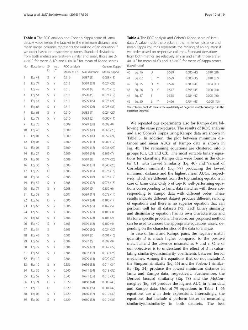
generated by using all of the Jamu pairs from match andmismatch efficacies. The Euclidean distance metric wasused to measure the distance from the (0, 1) point to the(FPR, TPR) points for all 45 selected equations. Inaddition, we created 20 ROC curves for each equationconsidering in each case the match class Jamu pairs andone of the 20 different mismatch class samples. Thus,we obtained 20 AUCs of the ROC curve for each equa-tion and averaged those values to determine the overallAUCs corresponding to an equation. The ROCR package[72] was used to calculate the AUC values. Table 4shows the results of ROC analysis and also Kappa scoresfor Jamu data. The scatter plot of minimum distancesand mean of AUCs corresponding to 45 equations forboth datasets is shown in Fig. 4. Based on the scatterplot generated using Jamu data in Fig. 4a, the 45

equations are empirically divided into 4 groups (C1, C2,C3, and C4). The well-performing equations correspond-ing to both approaches were obtained in C1, which con-sists of Eqs. 48, 49, 54, 68, and 79. The Michaelsimilarity (Eq. 68) produces the lowest minimum dis-tance, and the highest AUC is obtained by the Forbes-2similarity (Eq. 48). The ROC curves generated using Mi-chael and Forbes-2 similarities for all datasets are shownin Fig. 5. As expected, the ROC curves corresponding toall random datasets follow the diagonal line and thatcorresponding to Jamu data follows the above diagonalline. Most equations with the highest AUC values aresimilarity-measuring equations and these equations be-long to cluster III in Fig. 3. Out of these equations, theLance & Williams distance (Eq. 27) produces the highestAUC value among dissimilarity-measuring equations.

Fig. 3 The heatmap and dendrogram of remaining binary similarity and dissimilarity measures using Jamu data. The asterisk symbol (*) indicatesthe negative match quantity d is used in the equation


We repeated our experiments also for Kampo data fol-lowing the same procedures. The results of ROC analysisand also Cohen’s Kappa using Kampo data are shown inTable 5. In addition, the plot between minimum dis-tances and mean AUCs of Kampo data is shown inFig. 4b. The remaining equations are clustered into 3groups (C1, C2 and C3). The most suitable binary equa-tions for classifying Kampo data were found in the clus-ter C1, with Tarwid Similarity (Eq. 40) and Variant ofCorrelation similarity (Eq. 79) producing the lowestminimum distance and the highest mean AUCs, respect-ively, which are different from the top ranking equations incase of Jamu data. Only 5 of top-10 well-performing equa-tions corresponding to Jamu data matches with those cor-responding to Kampo data with different order. Theseresults indicate different dataset produce different rankingof equations and there is no superior equation that canperform well for all datasets [73]. Each binary similarityand dissimilarity equation has its own characteristics andfits for a specific problem. Therefore, our proposed methodcan be used to choose the appropriate equations wisely, de-pending on the characteristics of the data to analyze.In case of Jamu and Kampo pairs, the negative match

quantity d is much higher compared to the positivematch a and the absence mismatches b and c. One ofour objectives is to understand the effect of d in calcu-lating similarity/dissimilarity coefficients between herbalmedicines. Among the equations that do not include d,the Simpson similarity (Eq. 45) and the Forbes-1 similar-ity (Eq. 34) produce the lowest minimum distance inJamu and Kampo data, respectively. Furthermore, theDerived Jaccard similarity (Eq. 78) and the McCon-naughey (Eq. 39) produce the highest AUC in Jamu dataand Kampo data. Out of 79 equations in Table 1, 46equations use d in their expressions. Interestingly, theequations that include d perform better in measuringsimilarity/dissimilarity in both datasets. The best

Table 4 The ROC analysis and Cohen’s Kappa score of Jamudata. A value inside the bracket in the minimum distance andmean Kappa columns represents the ranking of an equation ifwe order based on respective columns. Standard deviationsfrom both metrics are relatively similar and small, those are 2-4×10-4 for mean AUCs and 0-6×10-4 for mean of Kappa scores

No Equations S/D

Incl.d*

ROC analysis Cohen’s Kappa

Mean AUCs Min. distance Mean Kappa

1 Eq. 48 S Y 0.616 0.587 (3) 0.088 (13)

2 Eq. 74 S Y 0.613 0.599 (29) 0.024 (28)

3 Eq. 49 S Y 0.613 0.588 (4) 0.076 (15)

4 Eq. 54 S Y 0.611 0.590 (5) 0.074 (19)

5 Eq. 44 S Y 0.611 0.599 (19) 0.073 (21)

6 Eq. 66 S Y 0.611 0.599 (26) 0.023 (31)

7 Eq. 68 S Y 0.610 0.583 (1) 0.024 (29)

8 Eq. 79 S Y 0.610 0.583 (2) 0.090 (11)

9 Eq. 78 S 0.609 0.599 (28) 0.092 (8)

10 Eq. 46 S 0.609 0.599 (20) 0.065 (23)

11 Eq. 01 S 0.609 0.599 (10) 0.052 (24)

12 Eq. 04 S 0.609 0.599 (11) 0.089 (12)

13 Eq. 06 S 0.609 0.599 (12) 0.036 (27)

14 Eq. 27 D 0.609 0.599 (14) 0.109 (7)

15 Eq. 02 S 0.609 0.599 (8) 0.074 (20)

16 Eq. 36 S 0.608 0.600 (31) 0.040 (25)

17 Eq. 29 D 0.608 0.599 (15) 0.076 (16)

18 Eq. 31 S 0.608 0.599 (16) 0.076 (17)

19 Eq. 57 S Y 0.608 0.599 (22) 0.076 (18)

20 Eq. 71 S Y 0.608 0.599 (9) 0.152 (6)

21 Eq. 39 S 0.607 0.599 (17) 0.078 (14)

22 Eq. 62 D Y 0.606 0.599 (24) 0.185 (1)

23 Eq. 63 S Y 0.606 0.599 (25) 0.167 (5)

24 Eq. 55 S Y 0.606 0.599 (21) 0.180 (3)

25 Eq. 61 S Y 0.606 0.599 (23) 0.183 (2)

26 Eq. 40 S Y 0.605 0.599 (18) 0.180 (4)

27 Eq. 34 S 0.605 0.600 (30) 0.024 (30)

28 Eq. 45 S 0.605 0.599 (7) 0.091 (10)

29 Eq. 52 S Y 0.604 0.597 (6) 0.092 (9)

30 Eq. 77 S Y 0.604 0.599 (27) 0.067 (22)

31 Eq. 51 S Y 0.604 0.602 (32) 0.039 (26)

32 Eq. 12 S 0.604 0.599 (13) 0.022 (32)

33 Eq. 10 S Y 0.556 0.656 (33) 0.014 (34)

34 Eq. 35 S Y 0.546 0.671 (34) 0.018 (33)

35 Eq. 59 S Y 0.545 0.671 (35) 0.013 (35)

36 Eq. 24 D Y 0.529 0.860 (44) 0.000 (43)

37 Eq. 15 D 0.529 0.680 (39) 0.004 (42)

38 Eq. 08 S Y 0.529 0.680 (37) 0.010 (39)

39 Eq. 09 S Y 0.529 0.680 (38) 0.010 (36)

Table 4 The ROC analysis and Cohen’s Kappa score of Jamudata. A value inside the bracket in the minimum distance andmean Kappa columns represents the ranking of an equation ifwe order based on respective columns. Standard deviationsfrom both metrics are relatively similar and small, those are 2-4×10-4 for mean AUCs and 0-6×10-4 for mean of Kappa scores(Continued)

40 Eq. 16 D 0.529 0.680 (40) 0.010 (38)

41 Eq. 07 S Y 0.529 0.680 (36) 0.010 (37)

42 Eq. 25 D Y 0.526 0.680 (41) 0.004 (41)

43 Eq. 26 D Y 0.517 0.895 (45) 0.000 (44)

44 Eq. 47 S 0.515 0.684 (42) 0.005 (40)

45 Eq. 50 S Y 0.466 0.754 (43) -0.008 (45)

The column "Incl. d" means the availability of negative match quantity d in theequation (Yes/No)


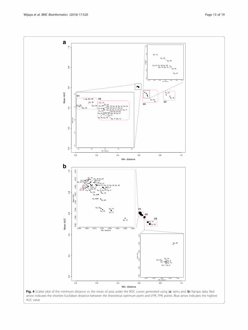
a

b

Fig. 4 Scatter plot of the minimum distance vs. the mean of area under the ROC curves generated using (a) Jamu and (b) Kampo data. Redarrow indicates the shortest Euclidean distance between the theoretical optimum point and (FPR, TPR) points. Blue arrow indicates the highestAUC value


Random Jamu

Random 1%Random 5%Random 10%

Jamu

False positive rate

True

posi

tive

rate

0.0 0.2 0.4 0.6 0.8 1.0

0.0

0.2

0.4

0.6

0.8

1.0

Random Jamu

JamuRandom 1%Random 5%Random 10%

False positive rate

True

posi

tive

rate

0.0 0.2 0.4 0.6 0.8 1.0

0.0

0.2

0.4

0.6

0.8

1.0

a

b

Fig. 5 The ROC curves of Michael and Forbes-2 similarities for Jamu and random datasets. a Michael similarity (Eq. 68). b Forbes-2 similarity (Eq. 48)


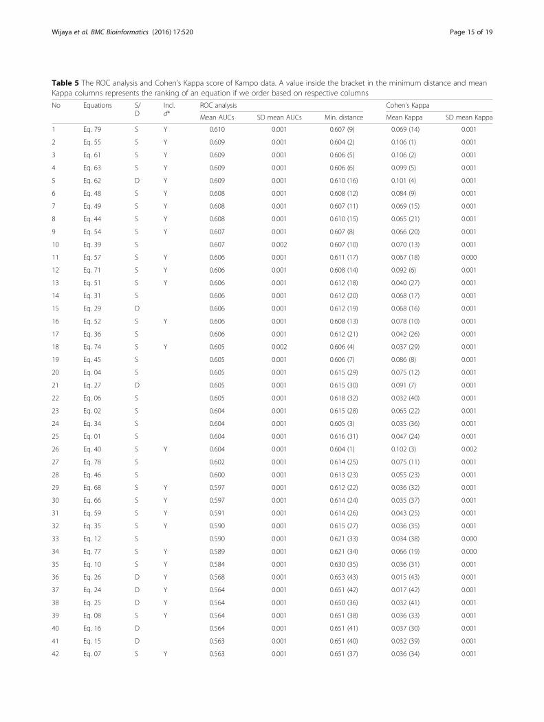
Table 5 The ROC analysis and Cohen’s Kappa score of Kampo data. A value inside the bracket in the minimum distance and meanKappa columns represents the ranking of an equation if we order based on respective columns

No Equations S/D

Incl.d*

ROC analysis Cohen’s Kappa

Mean AUCs SD mean AUCs Min. distance Mean Kappa SD mean Kappa

1 Eq. 79 S Y 0.610 0.001 0.607 (9) 0.069 (14) 0.001

2 Eq. 55 S Y 0.609 0.001 0.604 (2) 0.106 (1) 0.001

3 Eq. 61 S Y 0.609 0.001 0.606 (5) 0.106 (2) 0.001

4 Eq. 63 S Y 0.609 0.001 0.606 (6) 0.099 (5) 0.001

5 Eq. 62 D Y 0.609 0.001 0.610 (16) 0.101 (4) 0.001

6 Eq. 48 S Y 0.608 0.001 0.608 (12) 0.084 (9) 0.001

7 Eq. 49 S Y 0.608 0.001 0.607 (11) 0.069 (15) 0.001

8 Eq. 44 S Y 0.608 0.001 0.610 (15) 0.065 (21) 0.001

9 Eq. 54 S Y 0.607 0.001 0.607 (8) 0.066 (20) 0.001

10 Eq. 39 S 0.607 0.002 0.607 (10) 0.070 (13) 0.001

11 Eq. 57 S Y 0.606 0.001 0.611 (17) 0.067 (18) 0.000

12 Eq. 71 S Y 0.606 0.001 0.608 (14) 0.092 (6) 0.001

13 Eq. 51 S Y 0.606 0.001 0.612 (18) 0.040 (27) 0.001

14 Eq. 31 S 0.606 0.001 0.612 (20) 0.068 (17) 0.001

15 Eq. 29 D 0.606 0.001 0.612 (19) 0.068 (16) 0.001

16 Eq. 52 S Y 0.606 0.001 0.608 (13) 0.078 (10) 0.001

17 Eq. 36 S 0.606 0.001 0.612 (21) 0.042 (26) 0.001

18 Eq. 74 S Y 0.605 0.002 0.606 (4) 0.037 (29) 0.001

19 Eq. 45 S 0.605 0.001 0.606 (7) 0.086 (8) 0.001

20 Eq. 04 S 0.605 0.001 0.615 (29) 0.075 (12) 0.001

21 Eq. 27 D 0.605 0.001 0.615 (30) 0.091 (7) 0.001

22 Eq. 06 S 0.605 0.001 0.618 (32) 0.032 (40) 0.001

23 Eq. 02 S 0.604 0.001 0.615 (28) 0.065 (22) 0.001

24 Eq. 34 S 0.604 0.001 0.605 (3) 0.035 (36) 0.001

25 Eq. 01 S 0.604 0.001 0.616 (31) 0.047 (24) 0.001

26 Eq. 40 S Y 0.604 0.001 0.604 (1) 0.102 (3) 0.002

27 Eq. 78 S 0.602 0.001 0.614 (25) 0.075 (11) 0.001

28 Eq. 46 S 0.600 0.001 0.613 (23) 0.055 (23) 0.001

29 Eq. 68 S Y 0.597 0.001 0.612 (22) 0.036 (32) 0.001

30 Eq. 66 S Y 0.597 0.001 0.614 (24) 0.035 (37) 0.001

31 Eq. 59 S Y 0.591 0.001 0.614 (26) 0.043 (25) 0.001

32 Eq. 35 S Y 0.590 0.001 0.615 (27) 0.036 (35) 0.001

33 Eq. 12 S 0.590 0.001 0.621 (33) 0.034 (38) 0.000

34 Eq. 77 S Y 0.589 0.001 0.621 (34) 0.066 (19) 0.000

35 Eq. 10 S Y 0.584 0.001 0.630 (35) 0.036 (31) 0.001

36 Eq. 26 D Y 0.568 0.001 0.653 (43) 0.015 (43) 0.001

37 Eq. 24 D Y 0.564 0.001 0.651 (42) 0.017 (42) 0.001

38 Eq. 25 D Y 0.564 0.001 0.650 (36) 0.032 (41) 0.001

39 Eq. 08 S Y 0.564 0.001 0.651 (38) 0.036 (33) 0.001

40 Eq. 16 D 0.564 0.001 0.651 (41) 0.037 (30) 0.001

41 Eq. 15 D 0.563 0.001 0.651 (40) 0.032 (39) 0.001

42 Eq. 07 S Y 0.563 0.001 0.651 (37) 0.036 (34) 0.001


performing equations corresponding to minimum dis-tance and mean AUCs for Jamu data are Eqs. 68 and 48,which include negative match quantity d. Likewise, thebest equations in the Kampo data (Eqs. 79 and 40) alsoinclude negative match quantity d. Then, the top-5 wellperforming equations corresponding to both datasets in-clude d. If we also consider another metric to rank theclassifier performance, i.e. Cohen’s Kappa, we find a con-sistent result. That is top-5 equations with the largestKappa score also include d (Table 4 and 5). It impliesthe similarity between Jamu pairs and Kampo pairs areinfluenced by the negative matches. This result supportsthe findings of Zhang et al. [20] that all possible

matches, Sij where i, j ϵ{0,1}, should be considered forbetter classification results. Moreover, the performancemeasurement of binary similarity/dissimilarity equationsusing the AUC of ROC curve is more preferable to theminimum distance because this approach considers all(FPR, TPR) points, not only a single point with mini-mum distance to the optimum point.For further insight into the matter, we examined the

performance of the equations for every disease class inJamu data separately using the same approach. We cre-ated match and mismatch datasets for every disease classusing all Jamu pairs. The match class consists of Jamupairs with the same efficacy class and the mismatch class

Table 5 The ROC analysis and Cohen’s Kappa score of Kampo data. A value inside the bracket in the minimum distance and meanKappa columns represents the ranking of an equation if we order based on respective columns (Continued)

43 Eq. 09 S Y 0.563 0.001 0.651 (39) 0.037 (28) 0.001

44 Eq. 47 S 0.518 0.001 0.683 (44) 0.010 (44) 0.001

45 Eq. 50 S Y 0.501 0.001 0.702 (45) -0.004 (45) 0.000

The column "Incl. d" means the availability of negative match quantity d in the equation (Yes/No)

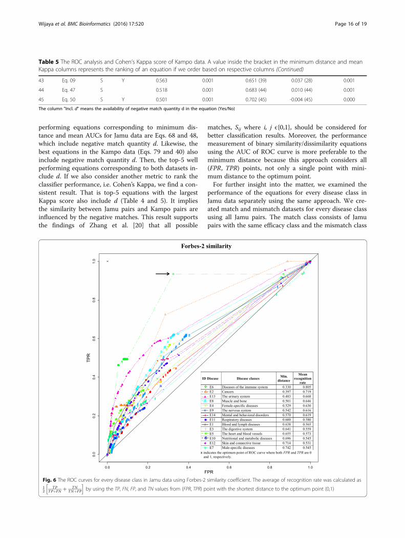
Fig. 6 The ROC curves for every disease class in Jamu data using Forbes-2 similarity coefficient. The average of recognition rate was calculated as12

TPTPþFN þ TN

TNþFP

h iby using the TP, FN, FP, and TN values from (FPR, TPR) point with the shortest distance to the optimum point (0,1)


consists of Jamu pairs with different efficacy class butone of the Jamu formulas in that pair has the same effi-cacy class as the match class. To measure the AUC ofROC curve, we created 20 mismatch classes each equalto the size of the match class by using the bootstrapmethod. Thus, we obtained 20 AUCs of the ROC curvesfor each disease class and each equation, and weaveraged those 20 values to determine the overall AUCscorresponding to a disease class and an equation(Additional file 1: Table S1). Figure 6 shows the ROCcurves for every disease class using Forbes-2 similaritycoefficients. The immune system disease class (E6) pro-duces the highest AUC score and the highest average ofAUCs (for all 45 equations). Moreover, the best classifi-cation is obtained in case of immune system class indi-cated by an arrow in Fig. 6, with the average ofrecognition rate of 0.805. The relatively high recognitionrate of E6 class corresponds to our knowledge that thedisease of immune system class is a very specific diseaseand utilization of the crude drug is restricted comparedto other disease classes. The minimum distance of anROC curve from the optimum point (expressed by Eq. 83)indicates the difficulty of classification i.e. the higher theminimum distance the more difficult it is to achieve a suc-cessful classification. Therefore, when the minimum dis-tance is close to zero, it implies that good classification ofthe data is possible. In case of classification of Jamu for-mulas concerning individual diseases, relatively lowerminimum distance was obtained for specific type of dis-ease classes such as diseases related to E6 and the urinarysystems (E13), which indicates that very specific types ofmedicinal plants are used to make such Jamu formulas.On the other hand, the disease classes such as those re-lated to digestive systems (E3) and nutritional and meta-bolic diseases (E10) are caused by diverse factors andtherefore the corresponding Jamu formulas are madeusing diverse types of plants resulting in relatively higherminimum distance for these disease classes (Fig. 6).

ConclusionsDifferent binary similarity and dissimilarity measures yielddifferent similarity/dissimilarity coefficients, which in turncauses differences in downstream analysis e.g. clustering.Hence, determining appropriate binary similarity and dis-similarity coefficients is an essential aspect of big data ana-lysis in versatile areas of scientific research includingchemometrics and bioinformatics. In this study, we pre-sented an organized way to select a suitable equation forstudying relationship between herbal medicine formulasin Indonesian Jamu and Japanese Kampo. We started ourstudy by collecting 79 binary similarity and dissimilarityequations from literature. In the early stages, we reducedalgebraically redundant equations and equations that pro-duce invalid values or relatively similar coefficients when

applied to our datasets. In addition, we eliminated someequations based on agglomerative hierarchical clusteringbecause they were very closely related to other equationsin the same cluster. Finally, we selected 45 unique equa-tions that produced different coefficients for our analysis.The ROC curve analysis was then performed to assess thecapabilities of these equations to separate herbal medicinepairs having the same and different efficacies. The experi-mental results show that the binary similarity and dissimi-larity measures that include the negative match quantity din their expressions have a better capability to separateherbal medicine pairs than those equations that exclude d.Moreover, we obtained different ranking of binary equa-tions for different datasets, i.e. Jamu and Kampo data.Thus, this result indicates the selection of binary similarityand dissimilarity measures is data dependent and weshould choose the binary similarity and dissimilarity mea-sures wisely depending on the data to be processed. Incase of Jamu data, the biggest AUC value is obtained bythe Forbes-2 similarity. Conversely, the Variant of Correl-ation similarity is recommended for classifying Kampopairs into match and mismatch classes. The procedurefollowed in this work can also be used to find suitable bin-ary similarity and dissimilarity measures under similar sit-uations in other applications.

Additional file

Additional file 1: Table S1. The mean of AUCs between equations anddisease classes in Jamu data. (XLSX 50 kb)

AbbreviationsAUC: The Area Under the ROC Curve; D: Dissimilarity; FN: False Negative;FP: False Positive; FPR: False Positive Rate; NA-DFC: The National Agency ofDrug and Food Control; NCBI: The National Center for BiotechnologyInformation; OTU: The Operational Taxonomic Unit; PR: Precision-Recall;ROC: The Receiver Operating Characteristic; S: Similarity; TCM: TraditionalChinese Medicine; TN: True Negative; TP: True Positive; TPR: True Positive Rate

AcknowledgementsNot applicable.

FundingThis work was supported by the National Bioscience Database Center inJapan; the Ministry of Education, Culture, Sports, Science, and Technology ofJapan; the US National Science Foundation and Japan Science andTechnology Agency [Strategic International Collaborative Research Program‘Metabolomics for a Low Carbon Society’]; the National Bioscience DatabaseCenter in Japan and NAIST Big Data Project.

Availability of data and materialsThe simulated dataset(s) supporting the conclusions of this article are availablein KNApSAcK Family Databases (http://kanaya.naist.jp/KNApSAcK_Family/).

Authors’ contributionsSW conducted the primary investigation, carried out the experiments,developed bmeasures package, and drafted the manuscript; SW, MA and SKdesigned the proposed method; FA provided Jamu-Species relations; MAand IB aided in the manuscript development; LD and SK supervised thestudy and participated in the manuscript. All authors read and approvedthe manuscript.


dx.doi.org/10.1186/s12859-016-1392-z

http://kanaya.naist.jp/KNApSAcK_Family/

Competing interestsThe authors declare that they have no competing interests.

Consent for publicationNot applicable.

Ethics approval and consent to participateNot applicable.

Author details1Graduate School of Information Science, Nara Institute of Science andTechnology, 8916-5 Takayama, Ikoma, Nara 630-0192, Japan. 2Department ofComputer Science, Bogor Agricultural University, Jl. Meranti Wing 20 Level 5Kampus IPB Dramaga, Bogor 16680, Indonesia. 3Department of Statistics,Bogor Agricultural University, Jl. Meranti Wing 22 Level 4 Kampus IPBDramaga, Bogor 16680, Indonesia. 4Tropical Biopharmaca Research Center,Bogor Agricultural University, Kampus IPB Taman Kencana, Jl. Taman KencanaNo. 3, Bogor 16128, Indonesia.

Received: 30 July 2016 Accepted: 29 November 2016

References1. Consonni V, Todeschini R. New similarity coefficients for binary data. Match-

Communications Math Comput Chem. 2012;68:581–92.2. Legendre P, Legendre L. Numerical ecology. 2nd. Amsterdam: Elsevier

Science; 1998.3. Batagelj V, Bren M. Comparing resemblance measures. J Classif. 1995;12:73–90.4. Afendi FM, Darusman LK, Hirai A, Altaf-Ul-Amin M, Takahashi H, Nakamura K,

Kanaya S: System biology approach for elucidating the relationship betweenIndonesian herbal plants and the efficacy of Jamu. In Proceedings - IEEEInternational Conference on Data Mining, ICDM. IEEE; 2010:661–668.

5. Afendi FM, Okada T, Yamazaki M, Hirai-Morita A, Nakamura Y, Nakamura K,Ikeda S, Takahashi H, Altaf-Ul-Amin M, Darusman LK, Saito K, Kanaya S:KNApSAcK family databases: Integrated metabolite-plant species databasesfor multifaceted plant research. Plant Cell Physiol 2012, 53:e1(1–12).

6. Auer J, Bajorath J. Molecular similarity concepts and search calculations. In:Keith JM, editor. Bioinformatics volume II: Structure, function andapplications (Methods in molecular biology), vol. 453. Totowa: HumanaPress; 2008. p. 327–47.

7. Kedarisetti P, Mizianty MJ, Kaas Q, Craik DJ, Kurgan L. Prediction andcharacterization of cyclic proteins from sequences in three domains of life.Biochim Biophys Acta - Proteins Proteomics. 2014;1844(1 PART B):181–90.

8. Zhou T, Shen N, Yang L, Abe N, Horton J, Mann RS, Bussemaker HJ, GordânR, Rohs R. Quantitative modeling of transcription factor binding specificitiesusing DNA shape. Proc Natl Acad Sci. 2015;112:4654–9.

9. Tibshirani R, Hastie T, Narasimhan B, Soltys S, Shi G, Koong A, Le QT. Sampleclassification from protein mass spectrometry, by “peak probability contrasts.Bioinformatics. 2004;20:3034–44.

10. Pinoli P, Chicco D, Masseroli M. Computational algorithms to predict GeneOntology annotations. BMC Bioinformatics. 2015;16 Suppl 6:1–15.

11. Kangas JD, Naik AW, Murphy RF. Efficient discovery of responses of proteinsto compounds using active learning. BMC Bioinformatics. 2014;15:1–11.

12. Ohtana Y, Abdullah AA, Altaf-Ul-Amin M, Huang M, Ono N, Sato T, SugiuraT, Horai H, Nakamura Y, Morita Hirai A, Lange KW, Kibinge NK, Katsuragi T,Shirai T, Kanaya S. Clustering of 3D-structure similarity based network ofsecondary metabolites reveals their relationships with biological activities.Mol Inform. 2014;33:790–801.

13. Abe H, Kanaya S, Komukai T, Takahashi Y, Sasaki SI. Systemization ofsemantic descriptions of odors. Anal Chim Acta. 1990;239:73–85.

14. Willett P, Barnard JM, Downs GM. Chemical similarity searching. J Chem InfModel. 1998;38:983–96.

15. Flower DR. On the properties of bit string-based measures of chemicalsimilarity. J Chem Inf Model. 1998;38:379–86.

16. Godden JW, Xue L, Bajorath J. Combinatorial preferences affect molecularsimilarity/diversity calculations using binary fingerprints and Tanimotocoefficients. J Chem Inf Model. 2000;40:163–6.

17. Agrafiotis DK, Rassokhin DN, Lobanov VS. Multidimensional scalingand visualization of large molecular similarity tables. J Comput Chem.2001;22:488–500.

18. Rojas-Cherto M, Peironcely JE, Kasper PT, van der Hooft JJJ, De Vos RCH,Vreeken RJ, Hankemeier T, Reijmers T. Metabolite identification usingautomated comparison of high-resolution multistage mass spectral trees.Anal Chem. 2012;84:5524–34.

19. Fligner MA, Verducci JS, Blower PE. A modification of the Jaccard–Tanimotosimilarity index for diverse selection of chemical compounds using binarystrings. Technometrics. 2002;44:110–9.

20. Zhang B, Srihari SN. Binary vector dissimilarity measures for handwritingidentification. In: Proceedings of SPIE-IS&T Electronic Imaging, vol. 5010.2003. p. 28–38.

21. Zhang B, Srihari SN. Properties of binary vector dissimilarity measures. In:Proc. JCIS Int’l Conf. Computer Vision, Pattern Recognition, and ImageProcessing. 2003. p. 1–4.

22. Kosman E, Leonard KJ. Similarity coefficients for molecular markers instudies of genetic relationships between individuals for haploid, diploid,and polyploid species. Mol Ecol. 2005;14(2):415–24.

23. Choi S-S, Cha S-H, Tappert CC. A survey of binary similarity and distancemeasures. J Syst Cybern Informatics. 2010;8:43–8.

24. Todeschini R, Consonni V, Xiang H, Holliday J, Buscema M, Willett P.Similarity coefficients for binary chemoinformatics data: Overview andextended comparison using simulated and real data sets. J Chem Inf Model.2012;52:2884–901.

25. Wijaya SH, Tanaka Y, Hirai A, Afendi FM, Batubara I, Ono N, Darusman LK,Kanaya S. Utilization of KNApSAcK Family Databases for Developing HerbalMedicine Systems. J Comput Aided Chem. 2016;17:1–7.

26. Seminar nasional dan pameran industri Jamu [http://seminar.ift.or.id/seminar-jamu-brand-indonesia/]. Accessed 19 Aug 2014.

27. Wijaya SH, Husnawati H, Afendi FM, Batubara I, Darusman LK, Altaf-Ul-AminM, Sato T, Ono N, Sugiura T, Kanaya S. Supervised clustering based onDPClusO: Prediction of plant-disease relations using Jamu formulas ofKNApSAcK database. Biomed Res Int. 2014;2014:1–15.

28. Okada T, Afendi FM, Yamazaki M, Chida KN, Suzuki M, Kawai R, Kim M, NamikiT, Kanaya S, Saito K. Informatics framework of traditional Sino-Japanesemedicine (Kampo) unveiled by factor analysis. J Nat Med. 2016;70:107–14.

29. da Silva MA, Garcia AAF, Pereira de Souza A, Lopes de Souza C. Comparisonof similarity coefficients used for cluster analysis with dominant markers inmaize (Zea mays L). Genet Mol Biol. 2004;27:83–91.

30. Demšar J. Statistical comparisons of classifiers over multiple data sets.J Mach Learn Res. 2006;7:1–30.

31. Lim T, Loh W, Shih Y. A comparison of prediction accuracy, complexity, andtraining time of thirty three old and new classification algorithms. MachLearn. 2000;40:203–29.

32. Metz CE. Basic principles of ROC analysis. Semin Nucl Med. 1978;8:283–98.33. Davis J, Goadrich M. The relationship between Precision-Recall and ROC

curves, Proc 23rd Int Conf Mach Learn – ICML’06. 2006. p. 233–40.34. Manning CD, Schütze H. Foundations of statistical natural language

processing. Cambridge: MITpress; 1999.35. Cohen J. A coefficient of agreement for nominal scales. Educ Psychol Meas.

1960;20:37–46.36. Ben-David A. A lot of randomness is hiding in accuracy. Eng Appl Artif Intell.

2007;20:875–85.37. Ben-David A. About the relationship between ROC curves and Cohen’s

kappa. Eng Appl Artif Intell. 2008;21:874–82.38. Genes and diseases [http://www.ncbi.nlm.nih.gov/books/NBK22185/].

Accessed 20 May 2016.39. Clifford HT, Stephenson W. An Introduction to Numerical Classification. New

York: Academic; 1975.40. Warrens MJ. Similarity coefficients for binary data: properties of coefficients,

coefficient matrices, multi-way metrics and multivariate coefficients.Psychometrics and Research Methodology Group, Leiden University Institutefor Psychological Research, Faculty of Social Sciences, Leiden University; 2008.

41. Jackson DA, Somers KM, Harvey HH. Similarity coefficients: Measures of co-occurrence and association or simply measures of occurrence? Am Nat.1989;133:436–53.

42. Dalirsefat SB, da Silva MA, Mirhoseini SZ. Comparison of similarity coefficientsused for cluster analysis with amplified fragment length polymorphismmarkers in the silkworm, Bombyx mori. J Insect Sci. 2009;9:1–8.

43. Jaccard P. The distribution of the flora in the alpine zone. New Phytol.1912;11:37–50.

44. Dice LR. Measures of the amount of ecologic association between species.Ecology. 1945;26:297–302.


http://seminar.ift.or.id/seminar-jamu-brand-indonesia/

http://seminar.ift.or.id/seminar-jamu-brand-indonesia/

http://www.ncbi.nlm.nih.gov/books/NBK22185/

45. Hubalek Z. Coefficients of association and similarity, based on binary(presence-absence) data: An evaluation. Biol Rev. 1982;57:669–89.

46. Cheetham AH, Hazel JE, Journal S, Sep N. Binary (presence-absence)similarity coefficients. J Paleontol. 1969;43:1130–6.

47. Cha S, Choi S, Tappert C. Anomaly between Jaccard and Tanimotocoefficients. In: Proceedings of Student-Faculty Research Day, CSIS, PaceUniversity. 2009. p. 1–8.

48. Cha S-H, Tappert CC, Yoon S. Enhancing Binary Feature Vector SimilarityMeasures. 2005.

49. Lourenco F, Lobo V, Bacao F. Binary-Based Similarity Measures forCategorical Data and Their Application in Self-Organizing Maps. 2004.

50. Ojurongbe TA. Comparison of different proximity measures andclassification methods for binary data. Faculty of Agricultural Sciences,Nutritional Sciences and Environmental Management, Justus LiebigUniversity Gießen; 2012.

51. Johnson SC. Hierarchical clustering schemes. Psychometrika. 1967;32:241–54.52. Michael EL. Marine ecology and the coefficient of association: A plea in

behalf of quantitative biology. J Ecol. 1920;8:54–9.53. Stiles HE. The association factor in information retrieval. J ACM. 1961;8(2):271–9.54. Nei M, Li W-H. Mathematical model for studying genetic variation in terms

of restriction endonucleases. Proc Natl Acad Sci U S A. 1979;76:5269–73.55. Holliday JD, Hu C-Y, Willett P. Grouping of coefficients for the calculation of

inter-molecular similarity and dissimilarity using 2D fragment bit-strings.Comb Chem High Throughput Screen. 2002;5:155–66.

56. Boyce RL, Ellison PC. Choosing the best similarity index when performingfuzzy set ordination on binary data. J Veg Sci. 2001;12:711–20.

57. Faith DP. Asymmetric binary similarity measures. Oecologia. 1983;57:287–90.58. Gower JC, Legendre P. Metric and Euclidean properties of dissimilarity

coefficients. J Classif. 1986;3:5–48.59. Chang J, Chen R, Tsai S. Distance-preserving mappings from binary vectors

to permutations. IEEE Trans Inf Theory. 2003;49:1054–9.60. Lance GN, Williams WT. Computer Programs for Hierarchical Polythetic

Classification (“Similarity Analyses”). Comput J. 1966;9:60–4.61. Avcibaş I, Kharrazi M, Memon N, Sankur B. Image steganalysis with binary

similarity measures. EURASIP J Appl Signal Processing. 2005;17:2749–57.62. Baroni-urbani C, Buser MW. Similarity of binary data. Syst Biol. 1976;25:251–9.63. Frigui H, Krishnapuram R. Clustering by competitive agglomeration. Pattern

Recognit. 1997;30:1109–19.64. Cimiano P, Hotho A, Staab S. Comparing conceptual, divisive and

agglomerative clustering for learning taxonomies from text. In: Ecai 2004:Proceedings of the 16th European Conference on Artificial Intelligence, vol.110. 2004. p. 435–9.

65. Bolshakova N, Azuaje F. Cluster validation techniques for genomeexpression data. Signal Process. 2003;83:825–33.

66. Bien J, Tibshirani R. Hierarchical clustering with prototypes via minimaxlinkage. J Am Stat Assoc. 2011;106(495):1075–84.

67. Sonego P, Kocsor A, Pongor S. ROC analysis: Applications to theclassification of biological sequences and 3D structures. Brief Bioinform.2008;9:198–209.

68. Fawcett T. An introduction to ROC analysis. Pattern Recognit Lett. 2006;27:861–74.69. Li M, Chen J, Wang J, Hu B, Chen G. Modifying the DPClus algorithm for

identifying protein complexes based on new topological structures. BMCBioinformatics. 2008;9:1–16.

70. Gorunescu F. Data Mining: Concepts, models and techniques. SpringerScience & Business Media, Verlag Berlin Heidelberg, Germany; 2011.

71. Carey VJ, Huber W, Irizarry RA, Dudoit S. Bioinformatics and ComputationalBiology Solutions Using R and Bioconductor. New York: Springer; 2005.

72. Sing T, Sander O, Beerenwinkel N, Lengauer T. ROCR: Visualizing classifierperformance in R. Bioinformatics. 2005;21:3940–1.

73. Gelbard R, Goldman O, Spiegler I. Investigating diversity of clusteringmethods: an empirical comparison. Data Knowl Eng. 2007;63:155–66. • We accept pre-submission inquiries

• Our selector tool helps you to find the most relevant journal

• We provide round the clock customer support

• Convenient online submission

• Thorough peer review

• Inclusion in PubMed and all major indexing services

• Maximum visibility for your research

Submit your manuscript atwww.biomedcentral.com/submit

Submit your next manuscript to BioMed Central and we will help you at every step:


finding an appropriate equation to measure similarity … · 2017-08-25 · finding an appropriate...

Documents