finding top-k elements in data streams - inesc-idfmmb/wiki/uploads/work/dict.refd.pdf · finding...

Information Sciences 180 (2010) 4958–4974

Contents lists available at ScienceDirect

Information Sciences

journal homepage: www.elsevier .com/locate / ins

Finding top-k elements in data streams

Nuno Homem ⇑, Joao Paulo CarvalhoTULisbon – Instituto Superior Técnico, INESC-ID, R. Alves Redol 9, 1000-029 Lisboa, Portugal

a r t i c l e i n f o

Article history:Received 10 November 2009Received in revised form 11 August 2010Accepted 15 August 2010

Keywords:Approximate algorithmsTop-k algorithmsMost frequentEstimationData stream frequencies

0020-0255/$ - see front matter � 2010 Elsevier Incdoi:10.1016/j.ins.2010.08.024

⇑ Corresponding author.E-mail addresses: [email protected] (N

a b s t r a c t

Identifying the most frequent elements in a data stream is a well known and difficult prob-lem. Identifying the most frequent elements for each individual, especially in very largepopulations, is even harder. The use of fast and small memory footprint algorithms is par-amount when the number of individuals is very large. In many situations such analysisneeds to be performed and kept up to date in near real time. Fortunately, approximateanswers are usually adequate when dealing with this problem. This paper presents anew and innovative algorithm that addresses this problem by merging the commonly usedcounter-based and sketch-based techniques for top-k identification. The algorithm pro-vides the top-k list of elements, their frequency and an error estimate for each frequencyvalue. It also provides strong guarantees on the error estimate, order of elements and inclu-sion of elements in the list depending on their real frequency. Additionally the algorithmprovides stochastic bounds on the error and expected error estimates. Telecommunicationscustomer’s behavior and voice call data is used to present concrete results obtained withthis algorithm and to illustrate improvements over previously existing algorithms.

� 2010 Elsevier Inc. All rights reserved.

1. Introduction

A data stream is a sequence of events or records that can be accessed in order of arrival, sometimes randomly, within asub-set of last arrivals or a period of time. The data stream model applies to many fields where huge data sets, possibly infi-nite, are generated and storage of the entire set is not viable. Applications such as IP session logging, telecommunicationrecords, financial transactions or real time sensor data generate so much information that the analysis has to be performedon the arriving data, in near real time or within a time window. In most cases, it is impossible to store all event details forfuture analysis due to the huge volume of data; usually only a set of summaries or aggregates is kept. Relevant information isextracted, transient or less significant data is dropped. In many cases those summaries have to be generated in a single passover the arriving data. Collecting and maintaining summaries over data streams require fast and efficient methods. Howeverapproximate answers may, in many situations, be sufficient.

Identifying the most frequent elements in a data stream is a critical but challenging issue in several areas. The challenge iseven bigger if this analysis is required at individual level, i.e., when a specific frequent elements list per individual is needed.This is essential when studying behavior and identifying trends. Some examples:

� Internet providers need to know the most frequent destinations in order to manage traffic and service quality;� Finding the most frequent interactions is critical to any social networking analysis as it provides the basic information of

connections and relations between individuals;

. All rights reserved.

. Homem), [email protected] (J.P. Carvalho).

http://dx.doi.org/10.1016/j.ins.2010.08.024

mailto:[email protected]

mailto:[email protected]

http://dx.doi.org/10.1016/j.ins.2010.08.024

http://www.sciencedirect.com/science/journal/00200255

http://www.elsevier.com/locate/ins

N. Homem, J.P. Carvalho / Information Sciences 180 (2010) 4958–4974 4959

� Telecommunication operators need to identify the most common call destinations for each customer for a variety of rea-sons, like classifying the customer in terms of marketing segmentation, proposing better and attractive customer deals,giving specific discounts for more frequently called numbers, or profiling the customer and detecting fraud situations orfraudsters that have returned under new identities;� Retail companies need to know the most common buys for each customer in order to better classify the customer and

target him with the appropriate marketing campaigns, to propose better and more attractive customer deals, to give spe-cific discounts for specific products, or to identify changes in spending profile or consumer habits.

Knowing the most frequent elements for each individual, or from their transactions, in a large population, is a quite distinctproblem from finding the most frequent elements in a large set. For each individual the number of distinct elements may notbe huge, but the number of individuals can be. Instead of a single large set of frequent elements, a large number of smallersets of frequent elements are required.

In many situations this information has to be kept up to date and available at any time. Accurately identifying it in nearreal time without allocating a huge amount of resources to the task is the problem. A data stream with multiple transactionsper day from several million individuals represents a huge challenge. Optimizing the process is therefore critical.

Classical exact top-k algorithms require checking the previous elements included in the list every time a new transactionis processed, either to insert new elements or to update the existing element counters. Exact top-k algorithms require largeamounts of memory as they need to store the complete list of elements. Storing a 1000 list of elements per each individual ifonly the top-20 is required is a complete waste of resources. Approximate, small footprint algorithms are the solution whenhuge numbers of individual lists are required. For example, Telecommunication operators can range from less than 500,000customers (a small operator) to more than 25,000,000 customers, and a list of the top-20 services or destinations might beneeded for each one; Retail sellers have similar or an even larger number of customers, in some cases identified by the use offidelity cards. The number of elements to be stored per customer is usually small as people tend to make frequent calls to arelatively small number of destinations and to frequently buy the same products.

This paper proposes a new algorithm for identifying the approximate top-k elements and their frequencies while provid-ing an error estimate for each frequency. The algorithm gives strong guarantees on the error estimate, on the order of ele-ments and on the inclusion of elements in the list depending on their real frequency. Stochastic error bounds that furtherimprove its performance are also presented. The algorithm was designed for reduced memory consumption as it is intendedto address the problem of solving a huge number of distinct frequent elements queries in parallel. It provides a fast updateprocess for each element, avoiding full scans or batch processing. Since the algorithm provides an error estimate for eachfrequency, it also provides the possibility to control the quality of the estimate.

Although the focus of the algorithm is to produce a large number of good top-k lists, each based on the individual set oftransactions, it can also be used to efficiently produce a single top-k list for a huge number of transactions.

The presented algorithm is innovative since it merges the two very distinct approaches commonly used to solve this sortof problems: counter-based techniques, and sketch-based techniques. It follows the principles presented by Metwally et al.[14] for Space-Saving algorithm but improves it quite significantly by narrowing down both the number of required coun-ters, update operations and the error associated with the frequency estimate. This is achieved by filtering elements using aspecially designed sketch. The merge of these two distinct approaches improves the existing properties of Space-Saving algo-rithm, providing lower stochastic bounds for estimate error and for the expected error.

In this work one also discusses how distinct implementation options can be used to minimize memory footprint and tobetter fit the algorithm and the corresponding data structures to the specific problem.

2. Typical behavior of mobile phone users

Although the algorithm is generic, it was originally developed to find top-k call destination numbers for each customer intelecommunications companies. Given the required precision in this situation, the use of approximate algorithms was con-sidered more than adequate. The typical behavior of individual customers is presented to illustrate the relevance of this anal-ysis. A set of real voice calls from mobile phone customers was used as a sample. As mobile phone users make more calls perday than landline phone users, this makes them ideal for use as a reference in this analysis.

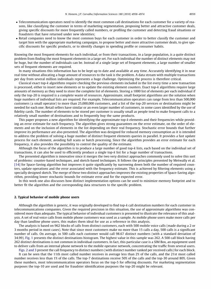
The analysis is based on 962 blocks of calls from distinct customers, each with 500 mobile voice calls (made during a 2 or3 months period in most cases). Note that since most customers make no more than 15 calls a day, 500 calls is a significantnumber of calls. On average, in 500 calls each customer would call 98.67 distinct numbers (with a standard deviation of34.99). Fig. 1 presents the distinct destinations histogram. The highest value in this sample was 262. A 500 call block having262 distinct destinations is not common in individual customers. In fact, this particular case is a SIM Box, an equipment usedto deliver calls from an internal phone network to the mobile operator network, concentrating the traffic from several users.

Figs. 2 and 3 present the call frequency to distinct numbers (with distinct number ranked per received calls) for each block.It can be seen that the 11th most called number receives in average less than 2% of the calls, and the 21st most called

number receives less than 1% of the calls. The top-7 destinations receive 50% of the calls and the top-30 around 80%. Giventhese numbers, most telecommunication operators focus on the top-5 for offering discounts. For marketing segmentationpurposes the top-10 are used and for fraudster identification purposes the top-20 might be relevant.

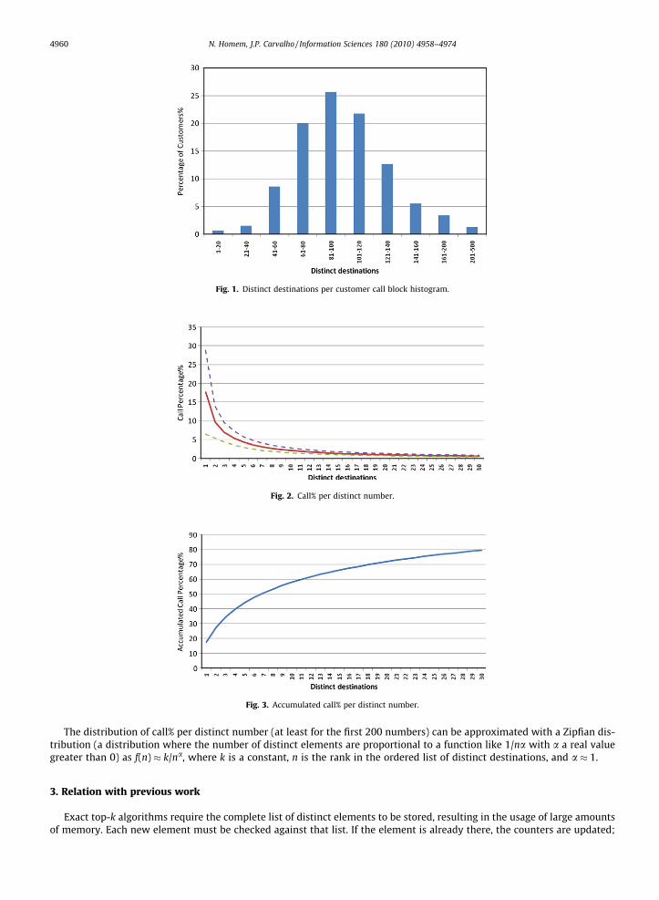
Fig. 1. Distinct destinations per customer call block histogram.

Fig. 2. Call% per distinct number.

Fig. 3. Accumulated call% per distinct number.

4960 N. Homem, J.P. Carvalho / Information Sciences 180 (2010) 4958–4974

The distribution of call% per distinct number (at least for the first 200 numbers) can be approximated with a Zipfian dis-tribution (a distribution where the number of distinct elements are proportional to a function like 1/na with a a real valuegreater than 0) as f(n) � k/na, where k is a constant, n is the rank in the ordered list of distinct destinations, and a � 1.

3. Relation with previous work

Exact top-k algorithms require the complete list of distinct elements to be stored, resulting in the usage of large amountsof memory. Each new element must be checked against that list. If the element is already there, the counters are updated;


otherwise the new element is inserted. To allow a fast search of the elements, hash tables or binary trees may be used, result-ing in an additional overhead in memory consumption.

Approximate algorithms can roughly be divided into two classes: Counter based techniques and Sketch-based techniques.

3.1. Counter based techniques

The most successful counter-based technique previously known, the Space-Saving algorithm, was proposed by Metwallyet al. in [14]. Space-Saving underlying idea is to monitor only a pre-defined number of m elements and their associated coun-ters. Counters on each element are updated to reflect the maximum possible number of times an element has been observedand the error that might be involved in that estimate. If an element that is already being monitored occurs again, the counterfor the frequency estimate is incremented. If the element is not currently monitored it is always added to the list. If the max-imum number of elements has been reached, the element with the lower estimate of possible occurences is dropped. Thenew element estimate error is set to the estimate of frequency of the dropped element. The new element frequency estimateequal to the error plus 1.

The Space-Saving algorithm will keep in the list all the elements that may have occurred at least the new estimate errorvalue (or the last dropped element estimate) of times. This ensures that no false negatives are generated but allows for falsepositives. Elements with low frequencies that are observed in the end of the data stream have higher probabilities of beingpresent in the list.

Since the Space-Saving algorithm maintains both the frequency estimate and the maximum error of this estimate, it alsomaintains implicitly the number of observed elements while the element was being monitored. Under some constraints, theorder of the top-k elements is guaranteed to be the correct one. By allowing m, the number of elements in the monitored list,to be larger than k, the algorithm provides good results in most cases. The need to allow for m to be much larger than k moti-vated the algorithm proposed in this paper.

Metwally et al. provide in [14] a comparison between several algorithms used to address this problem. It is shown thatthe Space-Saving algorithm is already less demanding on counters than other comparable algorithms, like Lossy Counting[13] or Probabilistic Lossy Counting [5]. These algorithms process the data stream in batches and require counters to be zer-oed at the end of each batch. This requires frequent scans of the counters and result in freeing space before it is really needed.Probabilistic Lossy Counting improves the rate of replacement of elements by using a probabilistic bound error instead of adeterministic value.

The Frequent algorithm, proposed in [4] and based on [15], outputs a list of k elements with no guarantee on which ele-ments, if any, have frequency higher than N/(k + 1), where N is the total number of elements. The Frequent algorithm uses kcounters to monitor k elements. If an element that is already being monitored occurs again, the counter for the frequencyestimate is incremented; else all counters are decremented. If a counter is zeroed, it is made free for the observed element.All free counters can be filled with the next observed values. The results are poor as no estimate is made on the frequency ofeach element.

The sampling algorithm Probabilistic-InPlace proposed in [4], in line with Sticky Sampling [13], also addresses the searchfor the top-k elements, but is unable to provide estimates of the frequency or any guarantees on order. It also requires morespace and processes elements in batches with counter deletions in the end of each batch.

A distinct approach, FDPM, is presented in [19]. FPDM focus in controlling the number of false negatives elements insteadof false positives. This minimizes the probability of missing a frequent element to be missed while keeping memory usageunder control. The main inconvenient is that more false positives may be included in the list.

3.2. Sketch-based techniques

Sketch-based algorithms use bitmap counters in order to provide a better estimate of frequencies for all elements. Eachelement is hashed into one or more values, those values are used to index the counters to update. Since the hash function cangenerate collisions, there is always a possible error. Keeping a large set of counters to minimize collision probability leads toan higher memory footprint when comparing with Space-Saving algorithm. Additionally, the entire bitmap counter needs tobe scanned and elements sorted to answer to the top-k query.

GroupTest proposed in [2], is a probabilistic approach based on FindMajority [2]. However it does not provide informationabout frequencies or relative order. Multistage filters were proposed as an alternative in [7] but present the same problems.Sketch-based algorithms are however very useful when it is necessary to process huge number of elements and extract asingle top-k list. The memory consumption of these algorithms usually depends on the number of distinct elements ofthe stream to ensure controlled collision rates. An experimental evaluation of some of the described algorithms is presentedin [12].

3.3. Related data mining techniques

In the data mining area there has been a huge amount of work focused on obtaining frequent itemsets in high volume andhigh-speed transactional data streams. The use of FP-trees (Frequent Pattern trees) and variations of the FP-growth algo-rithms to extract frequent itemsets is proposed in [16,11]. Frequent itemsets extraction in a sliding window is proposed


in [17]. Although the problem of extracting itemsets may be slightly different, the same algorithms may be used to extractfrequent elements.

4. The filtered Space-Saving algorithm (FSS)

In this work one proposes a novel algorithm, Filtered Space-Saving (FSS), that uses a filtering approach to improve onSpace-Saving [14]. It also gets some inspiration on previous work around probabilistic counting and sliding windows statis-tics [3,6,8–10,18]. FSS uses a bitmap counter to filter and minimize updates on the monitored elements list and also to betterestimate the error associated with each element. Instead of using a single error estimate value, it uses an error estimatedependent on the hash counter. This allows for better estimates by using the maximum possible error for that particularhash value instead of a global value. Although an additional bitmap counter has to be kept, it reduces the number of extraelements in the list needed to ensure high quality top-k elements. It will also reduce the number of list updates. The con-junction of the bitmap counter with the list of elements, minimizes the collision problem of most sketch-based algorithms.The bitmap counter size can depend on the number of k elements to be retrieved and not on the number of distinct elementsof the stream, which is usually much higher.

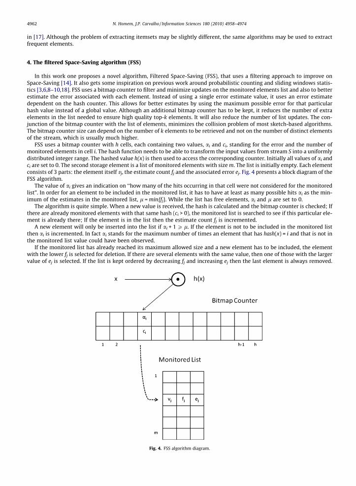
FSS uses a bitmap counter with h cells, each containing two values, ai and ci, standing for the error and the number ofmonitored elements in cell i. The hash function needs to be able to transform the input values from stream S into a uniformlydistributed integer range. The hashed value h(x) is then used to access the corresponding counter. Initially all values of ai andci are set to 0. The second storage element is a list of monitored elements with size m. The list is initially empty. Each elementconsists of 3 parts: the element itself vj, the estimate count fj and the associated error ej. Fig. 4 presents a block diagram of theFSS algorithm.

The value of ai gives an indication on ‘‘how many of the hits occurring in that cell were not considered for the monitoredlist”. In order for an element to be included in the monitored list, it has to have at least as many possible hits ai as the min-imum of the estimates in the monitored list, l = min{fj}. While the list has free elements, ai and l are set to 0.

The algorithm is quite simple. When a new value is received, the hash is calculated and the bitmap counter is checked; Ifthere are already monitored elements with that same hash (ci > 0), the monitored list is searched to see if this particular ele-ment is already there; If the element is in the list then the estimate count fj is incremented.

A new element will only be inserted into the list if ai + 1 P l. If the element is not to be included in the monitored listthen ai is incremented. In fact ai stands for the maximum number of times an element that has hash(x) = i and that is not inthe monitored list value could have been observed.

If the monitored list has already reached its maximum allowed size and a new element has to be included, the elementwith the lower fj is selected for deletion. If there are several elements with the same value, then one of those with the largervalue of ej is selected. If the list is kept ordered by decreasing fj and increasing ej then the last element is always removed.

Fig. 4. FSS algorithm diagram.


When the selected element is removed from the list, the corresponding bitmap counter cell is updated, cj is decreased and ai

is set with the maximum error incurred for that position in a single element, which corresponds to the estimate for the re-moved element, ai = fj.

The new element is included in the monitored list ordered by decreasing fj and increasing ej, ci is incremented, fj = ai + 1and ej = ai.

It is easy to see that the Space-Saving algorithm is a particular case of FSS when h = 1.Obvious optimizations to this algorithm, such as the use of better structures to hold the list of elements, to keep up to date

l, or to speed up access to each element will not be covered at this stage. Fig. 5 presents the proposed FSS algorithm.

5. Properties of filtered Space-Saving

FSS builds on the properties of Space-Saving algorithm and adds some very interesting stochastic guarantees for lowerbounds of error l and for the expected value of l.

Theorems 1–3 present strong guarantees inherited from Space-Saving algorithm. Theorems 4–7 present bounds on l andthe expected value of l, E(l), that allow error to be stochastically limited depending on the total number of elements N andthe number of cells h in the bitmap counter.

Lemma 1. The value of l and of each ai increases monotonically over time. For every t, t0 after the algorithm has been started:

t P t0 ) aiðtÞP aiðt0Þ ð1Þt P t0 ) lðtÞP lðt0Þ ð2Þ

Proof. As ai and l are integers:

ai þ 1 > l() ai P l

By construction whenever ai P l there is a replacement in the monitored list and there will be a new element insertedwhere fj = ai + 1. At that instant l will be updated to min{fj}, so:

aiðtÞ 6 maxfaiðtÞg 6 lðtÞ ¼ minffjðtÞg 6 fjðtÞ ð3Þ

Fig. 5. FSS algorithm.


Consider t1 as the moment before the replacement and t2the moment after the replacement, t2 > t1. If the replaced element inthe list was the only element to have fj(t1) = l(t1) then:

lðt2Þ ¼ aiðt1Þþ1 > lðt1Þ

If more than one element in the list had fj(t1) = l(t1) then

lðt2Þ ¼ lðt1Þ

Therefore in every situation:

lðt2ÞP lðt1Þ

In the replacement process, the cell in the bitmap corresponding to the hash of the replaced element will be updated withthe value of that element:

aiðt2Þ ¼ fkðt1Þ ¼ lðt1ÞP maxfaiðt1ÞgP aiðt1Þ

Whenever a new hit does not require a replacement in the list, one counter among the m counters for fj plus the h countersfor ai will be incremented. Therefore at all times:

t P t0 ¼> lðtÞP lðt0Þt P t0 ¼> aiðtÞP aiðt0Þ �

Lemma 2. The total number of elements N in the stream S is greater than or equal to estimated frequencies in the monitored list.Let Ni be the number of elements with hash equal to i from the stream S:

N ¼X

i

Ni PX

j

fj ð4Þ

Proof. When the element is being monitored, every hit in S increments at most one counter among the m counters for fj

when the element is being monitored. This is true even when a new element replaces an older one, as the new element fi

enters with exactly the older value plus the observed hit. h

Theorem 1. Among all counters, the minimum counter value, l, is no greater than N/m.

Proof. Since the total number of elements is always higher than the total of the m counters:

N ¼X

i

Ni PX

j

fj ¼X

j

ðfj � lÞ þX

j

l ¼X

j

ðfj � lÞ þml ð5Þ

and fj � l P 0, then:

l 6 N �X

j

ðfj � lÞ" #

=m 6 N=m � ð6Þ

Theorem 2. An element xi with Fi > l, where is Fi the real number of times xi appears in the stream S, must exist in the monitoredlist.

Proof. The proof is by contradiction. Assume xi is not in the monitored list. Then, all hits should have been counted in someai. Note that not even replacements of other elements in the list can lower ai so it would not be lower than Fi.

Since Fi > l, this would mean that ai P Fi > l which breaks the hypothesis, so xi should be in the list. h

Lemma 3. The value fi � ei is always the number of times an element was observed since it was included in the list. Denoting Fi asthe number of times that element xi was effectively in the stream S, the real frequency:

fi � ei 6 Fi 6 fi ð7Þ

Proof. The first part is trivial to prove as Fi may be greater or equal to the number the element has effectively registeredwhile it was monitored. To prove the second part, let one assume the opposite, i.e., Fi > fi. In this case, Fi > f-i > fi � ei + ei = Fi > fi � ei + l(t0), where t0 is the moment immediately before xi was included in the list. But this would meanthat at that moment t0, Fi(t0) > l(t0), which breaks the previous hypothesis. So Fi 6 fi. h

In fact FSS maintains all the properties of Space-Saving, inclusively the guarantee of a maximum error of the estimate.

Theorem 3. Whether or not xi occupies the ith position in the monitored list, fi, the counter at position i, is no smaller than Fi, thefrequency of the element with rank i, xi.


Proof. There are four possibilities for the position of xi.

1. The element xi is not monitored. Thus, from previous property, Fi 6 l. Thus any counter in the monitored list is no smallerthan Fi.

2. The element xi is at position j, such that j > i. Knowing that the estimate of xi is always bigger or equal to Fi, fj P Fi. Since j isgreater than i, then fi is no smaller than fj, the estimated frequency of xi. Thus, fi P Fi.

3. The element xi is at position i, so fi P Fi.4. The element xi is at position j, such that j < i. Thus, at least one element xu with rank u < i is located in some position y,

such that y P i. Since the estimated frequency of xu is no smaller than its frequency, Fu, and u < i, then the estimated fre-quency of xu is no smaller than Fi. Since y P i, then the fi P fy, which is equal to the estimated frequency of xu. Therefore,fi P Fi.

Therefore, in all cases, fi P Fi. h

As for Space-Saving, this is significant, since it enables estimating an upper bound on the rank of an element. The rank ofan element xi has to be less than j if the guaranteed hits of xi are less than the counter at position j. That isfj < (fi � ei)) rank(xi) < j. Conversely, the rank of an element xi is greater than the number of elements having guaranteeda number of hits larger than fi. That is, rank(xi) > count(xjj(fj � ej) > fi). This helps establishing the order-preservation propertyamong the top-k, as discussed later.

For FSS it can additionally be proven that l is limited by the distribution of hits in the bitmap counter:

Theorem 4. In FSS, for any cell that has monitored elements:

l 6 maxfNig ¼ Nmax; and ð8ÞEðlÞ 6 EðNmaxÞ ð9Þ

Proof. The use of a bitmap counter-based on a hash function that maps values into a pseudo-random uniformly distributedrange, gives the algorithm a probabilistic behavior. Let A be the monitored list, Ai the set of all elements in A such thathash(vj) = i and tj0 the moment element vj was inserted in the monitored list:

hashðv jÞ ¼ i ¼> ej ¼ aiðtj0Þ 6 aiðtÞ; t P tj0

The total number of elements N in stream S can be rewritten as the sum of Ni.

N ¼X

i

Ni

This means that, in fact, a few hits may be discarded when a replacement is done, and that Ni is greater than (if at least areplacement was done) or equal (no replacements) to ai plus the number of effective hits in monitored elements. Let A bethe monitored list and Ai the set of all elements in A such that hash(vj) = i:

Ni P ai þXj2Ai

ðfj � ejÞ

Ni P ai þXj2Ai

ðfj � ejÞP ai þXj2Ai

ðfj � aiÞÞP ai � ciai þXj2Ai

fj

Ni P ai � ciaiðt0Þ þXj2Ai

fj P ai � ciai þ cil

cil 6 Ni þ ðci � 1Þai 6 ciNi

For all ci > 0:

l 6 maxfNig

This means that the maximum estimate error l is lower than the maximum number of hits in any cell that has monitoredelements. It also means that for any i:

l 6 maxfNig ¼ Nmax

It is therefore trivial to conclude:
EðlÞ 6 EðNmaxÞ �
FSS has the very interesting property that error depends on the ratio between h and m and the number of samples N, andit can be guaranteed that this error is lower than in Space-Saving with a given probability. In fact for high values of N it givesa high probability of being much lower than Space-Saving. The following analysis considers a uniform distribution of ele-ments, this is one of the worst and possibly less interesting cases to identify top-k elements as the data is not skewedbut shows how the error bounds are improved by the bitmap counter filter.


Theorem 5. In FSS, assuming a uniform distribution of the elements x and a hash function with a pseudo-random uniformdistribution, the expected value of l, E(l), is a function of N, the number of elements in stream S and the number of elements h inbitmap counter.

EðlÞ 6 EðNmaxÞ ¼ NðCðN þ 1;N=hÞ=CðN þ 1ÞÞh �X

NPiP1

ðCði;N=hÞ=CðiÞÞh� ð10Þ

where C(x) is the complete gamma function and C(x,y) is the incomplete gamma function.

Proof. To estimate the Ni values in each cell, consider the Poisson approximation to the binomial distribution of the vari-ables as in [1]. One will assume that the events counted are received during the period of time T with a Poisson distribution.So:

k ¼ N=T

Or considering T = 1, the period of measure:

k ¼ N

This replaces the exact knowledge of N by an approximation as E(x) = N, with x = P(k). Although the expected value of thisrandom variable is the same as the initial value, the variance is much higher: it is equal to the expected value. This translatesin introducing a higher variance in the analysis of the algorithm. However, since the objective is to obtain a maximum bound,this additional variance can be considered.

Consider that the hash function h(x) distributes x uniformly over the h counters. The average rate of events falling incounter i can then be calculated as ki = k/h.

The probability of counter i receiving k events in [0,1] is given by:

PðNi ¼ kjt ¼ 1Þ ¼ Pikð1Þ ¼ kki e�kiT=k! ¼ ðN=hÞke�N=h=k!

And the cumulative distribution function is:

PðNi 6 kjt ¼ 1Þ ¼ Cðkþ 1;N=hÞ=Cðkþ 1Þ

To estimate E(Nmax) lets first consider the probability of having at least one Ni larger than k:

PðNmax 6 kjt ¼ 1Þ ¼ PðNi 6 k for all ijt ¼ 1Þ

As the Poisson distributions are infinitely divisible, the probability distributions and each of the resulting variables areindependent:

PðNmax 6 kjt ¼ 1Þ ¼Y

PðNi 6 kjt ¼ TÞ ¼Y

Cðkþ 1;N=hÞ=Cðkþ 1Þ ()

PðNmax 6 kjt ¼ 1Þ ¼ ½Cðkþ 1;N=hÞ=Cðkþ 1Þ�h ¼ gðkþ 1Þ

and since k is integer:

PðNmax ¼ kjt ¼ 1Þ ¼ PðNmax 6 kjt ¼ 1Þ � PðNmax 6 k� 1jt ¼ 1Þ () PðNmax ¼ kjt ¼ 1Þ

¼ ðCðkþ 1;N=hÞ=Cðkþ 1ÞÞh � ðCðk;N=hÞ=CðkÞÞh () PðNmax ¼ kjt ¼ 1Þ

¼ ½ðCðkþ 1;N=hÞ=kÞh � ðCðk;N=hÞÞh�=CðkÞh () EðlÞ 6 EðNmaxÞ

¼X

i

i½ðCðiþ 1;N=hÞ=Cðiþ 1ÞÞh � ðCði;N=hÞ=CðiÞÞh� () EðNmaxÞ ¼X

i

i½gðiþ 1Þ � gðiÞ�

¼ ½gð2Þ � gð1Þ� þ 2½gð3Þ � gð2Þ� þ � � � þ N½gðN þ 1Þ � gðNÞ� () EðNmaxÞ ¼ NgðN þ 1Þ �X

NPiP1

gðiÞ

¼ NðCðN þ 1;N=hÞ=CðN þ 1ÞÞh �X

NPiP1

ðCði;N=hÞ=CðiÞÞh� �

Theorem 5 allows h and N to be chosen so that the expected value for the maximum estimated error is as low as needed. Italso allows h and N to be chosen so that the maximum estimated error is as low as needed with a given probability u.

Figs. 6 and 7 illustrate the behavior of Ni and Nmax probability mass function using the N/h as the x axis. For N = 12,000 andh = 240:

For N = 120,000 and h = 240 the Ni function is relatively narrower and therefore Nmax approaches N/h = 1:Table 1 shows how the cumulative distribution function and the expected value for Nmax evolve with N.This gives an intuitive justification for using the error filter: the estimate error can be made lower than a certain value

(per example 120%) of N/h for large enough values of N by using more cells in the filter than in the monitored list (since eachentry in the monitored list requires space equivalent to at least 3 counters).

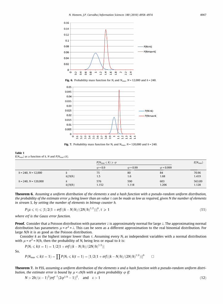
Fig. 6. Probability mass function for Ni and Nmax, N = 12,000 and h = 240.

Fig. 7. Probability mass function for Ni and Nmax, N = 120,000 and h = 240.

Table 1E(Nmax) as a function of k, N and P(Nmax6k).

P(Nmax 6 k) P u E(Nmax)

u = 0.9 u = 0.99 u = 0.999

h = 240, N = 12,000 k 75 80 84 70.96k/(N/h) 1.5 1.6 1.68 1.419

h = 240, N = 120,000 k 576 590 603 563.89k/(N/h) 1.152 1.118 1.206 1.128


Theorem 6. Assuming a uniform distribution of the elements x and a hash function with a pseudo-random uniform distribution,the probability of the estimate error l being lower than an value s can be made as low as required, given N the number of elementsin stream S, by setting the number of elements in bitmap counter h.

Pðl 6 sÞ 6 ½1=2ð1þ erf ððk� N=hÞ=ð2N=hÞ1=2ÞÞ�h; s P 1 ð11Þ

where erf is the Gauss error function.

Proof. Consider that a Poisson distribution with parameter k is approximately normal for large k. The approximating normaldistribution has parameters l = r2 = k. This can be seen as a different approximation to the real binomial distribution. Forlarge N/h it is as good as the Poisson distribution.

Consider k as the highest integer lower than s. Assuming every Ni as independent variables with a normal distributionwith l = r2 = N/h, then the probability of Ni being less or equal to k is:

PðNi 6 kjt ¼ 1Þ ¼ 1=2½1þ erf ððk� N=hÞ=ð2N=hÞ1=2Þ�
So, Y
PðNmax 6 kjt ¼ 1Þ ¼ PðNi 6 kjt ¼ 1Þ ¼ ½1=2ð1þ erf ððk� N=hÞ=ð2N=hÞ1=2ÞÞ�h �

Theorem 7. In FSS, assuming a uniform distribution of the elements x and a hash function with a pseudo-random uniform distri-bution, the estimate error is bound by l < eN/h with a given probability u if:

N > 2h=ðe� 1Þ2½erf�1ð2u1=h � 1Þ�2; and e > 1 ð12Þ

e is in fact the margin to consider when dimensioning h to achieve a given error with u probability when N elements are expected.


Proof. Consider u such that:

PðNmax 6 kjt ¼ 1ÞP u() PðNmax 6 kjt ¼ 1Þ ¼ ½1=2ð1þ erf ððk� N=hÞ=ð2N=hÞ1=2ÞÞ�h

P u() 1=2ð1þ erf ððk� N=hÞ=ð2N=hÞ1=2ÞÞP u1=h () erf ððk� N=hÞ=ð2N=h1=2ÞÞ

P 2u1=h � 1() ðk� N=hÞ=ð2N=hÞ1=2ÞP erf�1ð2u1=h � 1Þ

With k = eN/h:

ðeN=h� N=hÞ=ð2N=hÞ1=2Þ ¼ ðN=hÞ1=2ðe� 1Þ=ð2Þ1=2 P erf�1ð2u1=h � 1ÞN > 2h=ðe� 1Þ2½erf�1ð2u1=h � 1Þ�2 �

6. Frequent elements

This section presents the properties of FSS regarding answering frequent elements queries. It can be shown that in factFSS retains the properties of Space-Saving regarding given guarantees.

As in Space-Saving, in order to answer queries about the frequent elements, the monitored list is sequentially traverseduntil an element with frequency less than defined minimum frequency or support is found. This is proven by Metwally et al.in [14]. Frequent elements are reported in an ordered list of elements. An element, xi, is guaranteed to be a frequent elementif its guaranteed number of hits, fi � ei, exceeds ceil(uN), the minimum support. If for each reported element xi,fi � ei > ceil(uN), then the algorithm guarantees that all, and only the frequent elements are reported.

Answering frequent elements queries follow the Space-Saving algorithm. As for Space-Saving, assuming no specific datadistribution, FSS uses a number of counters m of:

minðjAj;1=eÞ ð13Þ
where jAj represents the number of elements in the monitored list, to find all frequent elements with error e. Any element, xi,with frequency Fi > uN is guaranteed to be reported. The proof is omitted as it follows Space-Saving and it has been proved inMetwally et al. [14]
For the more interesting case of noiseless Zipfian data with parameter a, to calculate the frequent elements with errorrate e, FFS follows Space-Saving and uses only:

minðjAj; ð1=eÞ1=a;1=eÞ counters ð14Þ
This is regardless of the stream permutation. The proof is omitted as it follows Space-Saving.
7. Top-k elements and order

For the top-k elements, the FSS algorithm can output the first k elements. An element, xi, is guaranteed to be among thetop-k if it’s guaranteed number of hits, fi � ei, exceeds fk+1, the over-estimated number of hits for the element in positionk + 1. Since, fk+1 is an upper bound on Fk+1, the hits of the element of rank k + 1, Ek+1, then xi is in the top-k elements.

The results have guaranteed top-k if by simply inspecting the results, the algorithm can determine that the reported top-kelements are correct. FSS and Space-Saving report a guaranteed top-k if for all i:

ðfi � eiÞP fkþ1 ð15Þ
where i 6 k.
That is, all the reported k elements are guaranteed to be among the top-k elements.In addition to having guaranteed top-k, the order of elements among the top-i elements are guaranteed to hold if the

guaranteed hits for every element in the top-k are more than the over-estimated hits of the next element.Thus, the order is guaranteed if the algorithm guarantees the top-i, for all i 6 k.Regardless of the data distribution, to solve the query of the approximate top-k in the stream S within an error e, FSS and

Space-Saving use:

minðjAj;N=eFkÞ counters ð16Þ

Any element with frequency higher than (1 � e)Fk is guaranteed to be monitored. The proof is omitted as it follows Space-Saving and it has been proved in Metwally et al. [14].

As for Space-Saving, assuming the data is noiseless Zipfian with parameter a > 1, to calculate the exact top-k, FSS uses:

minðjAj;Oððk=aÞ1=akÞÞ counters ð17Þ

When a = 1, the space complexity is:

minðjAj;Oðk2lnðjAjÞÞÞ ð18Þ

This is regardless of the stream permutation. Also, the order among the top-k elements is preserved. The proof is omitted as itfollows Space-Saving and it has been proved in Metwally et al. [14].


8. Implementation

The practical implementation of FSS may include the Stream-Summary data structure presented in [14]. An index by hashcode may be used to speed up searches (a binary search may be used), but depending on the number of elements in the mon-itored list, other options may as well be used. For small number of m (a few tens of elements), a simple array of m elements canbe a viable and fast option. To speed up insertions and replacements, an additional array with the indexes of each elementordered by fi may be used. This trades some performance for a very compact implementation. This may be the preferred optionfor telecommunication related implementations where the total number of elements in the list to be kept is 50 or even less.

Any implementation of FSS has to use a bitmap counter to hold the ai counters. The ci counters are however optional asthey may well be replaced by a single bit indicating the existence or not of elements in the monitored list with that hashcode. When an element is removed the bit is kept set. If the following search of element with hash i do not find an elementthen the bit is cleared. This reduces memory at the expense of a potential additional search in the monitored list (one thatSpace-Saving would always do anyway). Eventually ci counters may even be dropped at the expense of a search in the mon-itored list for every element in the stream S.

A further improvement in the memory usage of FSS can be made by using filter counters smaller than the counters neededfor the monitored list. In the above example, with N = 120,000, 17 bits would be needed for the monitored list counters. Forthe filter, only counters that map values between min{Ni} and max{Ni} are required, since all counters can be decremented bymin{Ni}, and the common factor min{Ni} stored in a single variable.

Using a similar approach to the max{Ni}, it can be seen that Nmin = max{Ni} has the following behavior:

PðNmin > kjt ¼ 1Þ ¼Yð1� PðNi 6 kjt ¼ 1ÞÞ ¼ ð1� PðNi 6 kjt ¼ TÞÞh () PðNmin > kjt ¼ 1Þ

¼ ð1� Cðkþ 1;N=hÞ=Cðkþ 1ÞÞh ð19Þ

Since E(Ni) � Nmin 6 Nmax � E(Ni) due to Poisson distribution properties:

maxfNig �minfNig 6 2½Nmax � EðNiÞ� ¼ 2Nmax � 2N=h ð20Þ

For the example with N = 120,000, the value of Nminwill be greater than 403 with probability 0.999. This means that a counterwith a range of 256 will be more than enough to hold the max{Ni} �min{Ni} value with a very high probability. It also meansthat a counter could have only 8 bits instead of 17 and therefore a single entry in the monitored list could be transformed in 6cells for filtering.

In this case the estimate error for N > 120,000 and h = 240 with probability 0.999 will be lower than:

l 6 Nmax � 1:206 N=h ¼ 603 ð21Þ

To ensure a similar error with Space-Saving, m = 120,000/603 � 199 would be needed. This would require 3 � 199 = 597counters of 17 bits each. FSS requires 240 counters of 8 bits each (equivalent to roughly 40 entries in Space-Saving), plusenough entries in the monitored list to hold at least the intended top-k values. This is in fact much less space than the re-quired for Space-Saving at the expense of a very small probability of error.

In fact experimental results show that the l will usually be significantly lower than Nmax. Another interesting finding fromexperiments is that the filter cells can in fact misrepresent Nmin and allow for cell underflow (by discarding very low andimprobable values of Ni due to insufficient counter range as Nmax increases) without significant impacts in the error estimate.

When the element identifier has the same size as the counters, Space-Saving, requires 3 variables for each entry in the list.Memory usage is still increased by the need of pointers for the Stream-Summary structure (as described in [14]). Using in-dexes instead of pointers will further reduce this. When using c bits per counter, Space-Saving will need 3 counters for eachentry plus m counters with log2m bits (the indexes only need to store values from 0 to m � 1):

SSSðmÞ � 3m c þm log2 m bits ð22Þ

FSS requires the same 3m counters for element storage plus an index and h counters plus a single bit. The counters in thefilter can however be smaller. For the filter only counters that map values between min{Ni} and max{Ni} are required asall counters can always be decremented by min{Ni}. For most situations counters can have half the size of the counters inthe monitored list, b = c/2. This can be resumed in:

SFSSðmÞ � 3m c þm log2 mþ hðc=2þ 1Þ ð23Þ

The practical dimensioning rule used in the following experiments was to trade 1 element in the Space-Saving monitored listfor 6 counters in the filter table. This would keep half the list and change the rest for filter. So with h = 6m and with c > > 1:

SSSðmSSÞ=SFSSðmFSSÞ � 1) mFSS � 1=2mSS ð24Þ

9. Experimental results

The first set of tests with Space-Saving and FSS try to show the performance of both algorithms in a typical telecommu-nications scenario where the top-10 or top-20 destinations are needed per customer. This does not require a huge number of


elements in the monitored list since the number of destinations on a typical customer is relatively small: as previouslyshown, in 500 calls an average 98 distinct destinations is expected. As most of the traffic is made to the top-10 or top-20destinations, these lists are enough for most practical purposes (either fraud or marketing related). As also previously said,500 is a large enough sample of calls, since most users will take more than a month to make 500 voice calls.

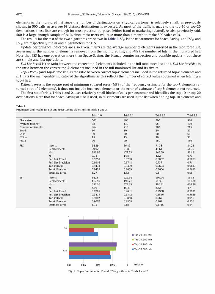
The results for the test of the two algorithms are shown in Table 2. SSm is the m parameter for Space-Saving, and FSSm andFSSh are respectively the m and h parameters for FSS.

Update performance indicators are also given. Inserts are the average number of elements inserted in the monitored list,Replacements the number of elements removed from the monitored list, and Hits the number of hits in the monitored list.Note that FSS has one operation more than Space-Saving, the bitmap counter inspection and possible update – but theseare simple and fast operations.

Full List Recall is the ratio between the correct top-k elements included in the full monitored list and i, Full List Precision isthe ratio between the correct top-k elements included in the full monitored list and its size m.

Top-k Recall (and Top-k Precision) is the ratio between correct top-k elements included in the returned top-k elements andk. This is the main quality indicator of the algorithms as this reflects the number of correct values obtained when fetching atop-k list.

Estimate error is the square root of minimum squared error (MSE) of the frequency estimate for the top-k elements re-turned (out of k elements). It does not include incorrect elements or the error of estimate of top-k elements not returned.

The first set of trials, Trials 1 and 2, uses relatively small blocks of calls per customer and identifies the top-10 or top-20destinations. Note that for Space-Saving m = 3k is used, so 30 elements are used in the list when finding top-10 elements and

Table 2Parameters and results for FSS ans Space-Saving algorithms in Trials 1 and 2.

Trial 1.0 Trial 1.1 Trial 2.0 Trial 2.1

Block size 500 800 500 800Average Distinct 98 130 98 130Number of Samples 962 715 962 715Top-k 10 10 20 20SS m 30 30 60 60FSS m 15 15 30 30FSS h 90 90 180 180

FSS Inserts 54.89 66.89 71.38 84.23Replacements 39.92 51.89 41.61 54.35Hits 296.86 477.73 346.69 561.91M 9.73 14.8 4.52 6.73Full List Recall 0.9758 0.9768 0.9892 0.9893Full List Precision 0.6916 0.6748 0.737 0.71Top-k Recall 0.9433 0.9409 0.9604 0.9633Top-k Precision 0.9433 0.9409 0.9604 0.9633Estimate Error 1.27 1.52 0.81 0.95

SS Inserts 142.8 222.64 109.94 161.3Replacements 112.95 192.71 51.39 101.88Hits 356.16 577.35 386.41 636.46M 8.96 15.39 2.52 4.7Full List Recall 0.9705 0.9631 0.9958 0.9931Full List Precision 0.3475 0.3342 0.3856 0.3629Top-k Recall 0.9002 0.8858 0.967 0.956Top-k Precision 0.9002 0.8858 0.967 0.956Estimate Error 1.35 2.18 0.3715 0.64

Fig. 8. Top-k Precision for SS and FSS algorithms in Trials 1 and 2.


60 when finding top-20 elements. Note that this is a significant size for the list, as an average of 98 distinct numbers in a 500call block is expected (130 in an 800 call block).

In these trials it can be observed that both Top-k Recall and Top-k Precision of FSS are marginally better than that ofSpace-Saving for top-10. It is interesting to see that in the top-20 trial the results are much closer. In fact, Space-Saving withm = 60 is able to store a large part of the distinct values and therefore the improvement of FSS is not relevant.

Table 3Parameters and execution results for Trial 3.

Trial 3.0 Trial 3.1 Trial 3.2

Block size 5000 10,000 20,000Average distinct 3130 5322 8774Number of samples 166 83 41Top-k 20 20 20SS m 200 200 200FSS m 100 100 100FSS h 600 600 600

FSS Inserts 1103.32 1921.33 3519.17Replacements 1003.32 1821.33 3419.17Hits 393.01 780.09 1522.68l 13.79 25.4 48.41Full List Recall 0.6287 0.6153 0.5775Full List Precision 0.1552 0.1386 0.1217Top-k Recall 0.4996 0.4686 0.4439Top-k Precision 0.4996 0.4686 0.4439Estimate error 5.57 9.97 18.47

SS Inserts 4234.83 8457.69 16941.8Replacements 4034.83 8257.69 16741.8Hits 765.16 1542.3 3058.19l 23.92 48.86 98.8Full List Recall 0.4278 0.3701 0.3376Full List Precision 0.0528 0.0419 0.0356Top-k Recall 0.2539 0.1987 0.1585Top-k Precision 0.2539 0.1987 0.1585Estimate error 14.87 31.09 63.82



Block size 5000 10,000 20,000Average distinct 3130 5322 8774Number of samples 166 83 41Top-k 20 20 20

FSS m = 100,h = 600 l 13.79 25.4 48.41Top-k Recall and Precision 0.4996 0.4686 0.4439Estimate error 5.57 9.97 18.47

m = 200,h = 1200 l 8.04 14.48 27.07Top-k Recall and Precision 0.7894 0.7734 0.7597Estimate error 2.36 3.37 5.34

m = 300,h = 1800 l 5.99 10.51 19.36Top-k Recall and Precision 0.8858 0.8951 0.889Estimate error 1.44 2.179 2.6

m = 400,h = 2400 l 5 8.92 15.97Top-k Recall and Precision 0.9246 0.9265 0.939Estimate error 1.25 1.57 2.019

SS m = 200 l 23.92 48.86 98.8Top-k Recall and Precision 0.2539 0.1987 0.1585Estimate error 14.87 31.09 63.82

m = 400 l 11.84 23.91 48.87Top-k Recall and Precision 0.4987 0.4138 0.3402Estimate error 4.71 9.5 18.12

m = 600 l 7.46 15.79 32.07Top-k Recall and Precision 0.7322 0.6192 0.5583Estimate error 1.82 4.4055 7.87

m = 800 l 5 11.42 23.82Top-k Recall and Precision 0.853 0.7903 0.7329Estimate error 1.25 2.12 4.08

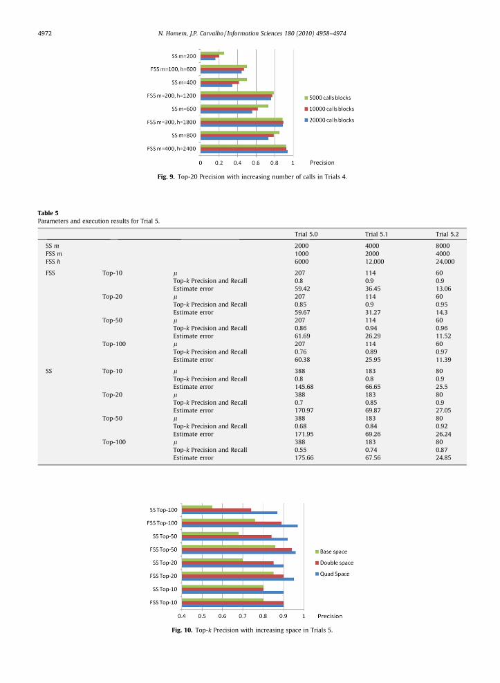
Fig. 9. Top-20 Precision with increasing number of calls in Trials 4.



SS m 2000 4000 8000FSS m 1000 2000 4000FSS h 6000 12,000 24,000

FSS Top-10 l 207 114 60Top-k Precision and Recall 0.8 0.9 0.9Estimate error 59.42 36.45 13.06

Top-20 l 207 114 60Top-k Precision and Recall 0.85 0.9 0.95Estimate error 59.67 31.27 14.3



SS Top-10 l 388 183 80Top-k Precision and Recall 0.8 0.8 0.9Estimate error 145.68 66.65 25.5




Fig. 10. Top-k Precision with increasing space in Trials 5.



Note also that the number of update operations in the monitored list is significantly lower for FSS.Fig. 8 presents Top-k Precision for both SS and FSS algorithms in Trials 1 and 2.The following block of trials, Trials 3, compares SS with FSS for a larger number of calls. In this case the calls are not from a

single user but calls made in a consecutive period of time. Increasing the time period gives us more calls. In this case only thetop-20 elements are found. The number of distinct elements per block of calls is now much higher so m and h increased pro-portionally for both algorithms. Table 3 shows the results for this second block of trials:

The absolute results are not reasonable for practical purposes, but the behavior of each algorithm is now more evident.Anyway only a very small list of elements is being used when compared to the number of distinct values in the sample (thelist is less than 6.4% the number of distinct elements). Space-Saving with m = 200 is only able to find 25.39% of the top-20elements when returning the first 20 elements in the list for 5000 calls and degrades significantly the performance when Nincreases. On the other hand, FSS is able to find nearly half of the top-20 elements and its performance degrades less when Nincreases.

Table 4 and Fig. 9 present the results for Trials 4, with an increasing value of m.Overall, the performance of FSS is consistently better than that of Space-Saving for similar memory usage. A very relevant

aspect is that FSS performance does not degrades with the increasing number of calls as in the case of Space-Saving.FSS with m = 200 and h = 1200, for N = 20,000, behaves better than Space-Saving with m = 800 that uses the double of the

space.Also important, FSS performance for larger blocks of calls improves more than for smaller blocks as the overall space allo-

cation increases (for m = 100, h = 600 performance is better for 5000 calls blocks than for 2000, for m = 400, h = 2400, it is theinverse). This is due to the behavior of the stochastic filtering of error, the ratio between Ni and Nmaxis reduced as the numberof calls increases (as shown in Figs. 6 and 7).

Table 5 and Fig. 10 show the results for Trials 5 when using the whole set of calls, with N = 800,000, totaling 112,462 dis-tinct values. It can be seen that FSS is consistently better than SS for similar memory usage.

10. Conclusions

This paper presents a new algorithm that builds on top of the best existing algorithm for answering the top-k problem. Iteffectively merges the best properties of two distinct approaches to this problem, the counter-based techniques and sketch-based ones. The new algorithm keeps the already excellent guarantees provided by Space-Saving algorithm regarding inclu-sion of elements in the answer, ordering of elements, maximum estimation error and provides probabilistic guarantees ofincreased precision.

The FSS algorithm filters and splits the error of Space-Saving algorithm through the use of a bitmap counter. It is alsoshown that this approach minimizes the operations of update of the monitored elements list by avoiding elements withinsufficient hits being inserted in the list. This helps to minimize the overall error and therefore the error associated witheach element. It eliminates the excess of trail elements from the data stream that Space-Saving usually includes in the mon-itored list and that have a very high estimation error.

Although FSS requires an additional bitmap counter, smaller counters are used overall allowing a trade-off. By replacingsome of the entries in the Space-Saving monitored list by additional cells in this bitmap counter it is possible to keep thesame space but have better expected performance out of the algorithm. In this paper a single entry in the monitored listwas exchanged for 6 additional cells in the bitmap counter. This seems to be a reasonable exchange rate specially if one con-siders the usual counter size (Space-Saving implementations usually use either 16 or 32 bits counters, FSS may use 8 bit or16 bit counters). This exchange rate coupled to the probabilistic guarantees of FSS (especially for large values of N, the streamsize) achieves better results. In fact FSS exchanges deterministic guarantees for tighter probabilistic ones.

This paper presents experimental results that detail improvements over Space-Saving algorithm, both in precision and inperformance when using similar memory space. Memory consumption was key in the analysis, since the practical problembeing solved is memory bound. In this regard, the use of FSS is envisioned with even less memory than Space-Saving andwith better precision. Although execution time will depend on specific aspects of the implementation, the number of oper-ations required by each algorithm was also detailed and points to reductions in execution time.

FSS is a low memory footprint algorithm that can answer not only the top-k problem for large number of transactions butalso the problem of answering huge number of top-k problems for a relatively small number of transactions. As such, itsapplicability goes much beyond telecommunications or retail applications. It can be used in any other domain as long asthe appropriate implementation choices and dimensioning are made.

Acknowledgement

This work was in part supported by FCT (INESC-ID multi annual funding) through the PIDDAC Program funds.

References

[1] D. Bertsekas, Dynamic Programming and Optimal Control, Vol. 1, Athena Scientific, 1995.[2] G. Cormode, S. Muthukrishnan. What’s Hot and What’s Not: TrackingMost Frequent Items Dynamically, in: Proceedings of the 22nd ACM PODS

Symposium on Principles of Database Systems, Pages 296–306, 2003.


[3] M. Datar, A. Gionis, P. Indyk, R. Motwani, Maintaining Stream Statistics Over Sliding Windows, SIAM Journal on Computing 31 (6) (2002).[4] E. Demaine, A. López-Ortiz, J. Munro. Frequency Estimation of Internet Packet Streams with Limited Space, in: Proceedings of the 10th ESA Annual

European Symposium on Algorithms, Pages 348–360, 2002.[5] X. Dimitropoulos, P. Hurley, A. Kind, Probabilistic lossy counting: an efficient algorithm for finding heavy hitters, ACM SIGCOMM Computer

Communication Review 38 (1) (2008).[6] C. Estan, G. Varghese. New directions in traffic measurement and accounting, in: Proceedings of SIGCOMM 2002 (2002), ACM Press. (Also: UCSD

technical report CS2002-0699, February, 2002; available electronically).[7] C. Estan, G. Varghese, New directions in traffic measurement and accounting: focusing on the elephants, ignoring the mice, ACM Transactions on

Computer Systems 21 (3) (2003) 270–313.[8] C. Estan, G. Varghese, M. Fisk, Bitmap algorithms for counting active flows on high speed links. Technical Report CS2003-0738, UCSD, 2003.[9] L. Fan, P. Cao, J. Almeida, A. Broder, Summary cache: a scalable wide-area web cache sharing protocol, IEEE/ACM Transactions on Networking 8 (3)

(2000) 281–293, doi:10.1109/90.851975.[10] P. Flajolet, N. Martin, Probabilistic counting algorithms for data base applications, Journal of Computer and System Sciences 31 (2) (1985).[11] T. Hu, S. Sung, H. Xiong, Q. Fu, Discovery of maximum length frequent itemsets, Information Sciences 178 (2008) 69–87.[12] N. Manerikar, T. Palpanas, Frequent items in streaming data: an experimental evaluation of the state-of-the-art, Data & Knowledge Engineering 68 (4)

(2009) 415–430.[13] G. Manku, R. Motwani. Approximate Frequency Counts over Data Streams, in: Proceedings of the 28th ACM VLDB International Conference on Very

Large Data Bases, pages 346–357, 2002.[14] A. Metwally, D. Agrawal, A. Abbadi, Efficient Computation of Frequent and Top-k Elements in Data Streams, Technical Report 2005-23, University of

California, Santa Barbara, 2005.[15] J. Misra, D. Gries, Finding repeated elements, Science of Computer Programming 2 (1982) 143–152.[16] S. Tanbeer, C. Ahmed, B. Jeong, Y. Lee, Efficient single-pass frequent pattern mining using a prefix-tree, Information Sciences 179 (5) (2009) 559–583.[17] S. Tanbeer, C. Ahmed, B. Jeong, Y. Lee, Sliding window-based frequent pattern mining over data streams, Information Sciences 179 (22) (2009) 3843–

3865.[18] K. Whang, B. Vander-Zanden, H. Taylor, A linear-time probabilistic counting algorithm for database applications, ACM Transactions on Database

Systems 15 (2) (1990).[19] J. Yu, Z. Chong, H. Lu, Z. Zhang, A. Zhou, A false negative approach to mining frequent itemsets from high speed transactional data streams, Information

Sciences 176 (2006) 1986–2015.

http://dx.doi.org/10.1109/90.851975

finding top-k elements in data streams - inesc-idfmmb/wiki/uploads/work/dict.refd.pdf · finding...

Documents