fine guidance sensor instrument handbook for cycle 25 table of contents 6.2 instrument...

Operated by the Association of Universities for Research in Astronomy, Inc., for the National Aeronautics and Space Administration

3700 San Martin DriveBaltimore, Maryland 21218

[email protected]

Version 26.0May 2018

Fine Guidance Sensor Instrument Handbook for Cycle 26

mailto:[email protected]

Send comments or corrections to:Space Telescope Science Institute

3700 San Martin DriveBaltimore, Maryland 21218

E-mail:[email protected]

User SupportPlease contact the HST Help Desk for assistance. We encourage users to access the newweb portal where you can submit your questions directly to the appropriate team ofexperts.

• Web portal: http://hsthelp.stsci.edu• E-mail: [email protected]• Phone: (410) 338-1082 or 1-800-544-8125

World Wide WebInformation and other resources are available on the FGS World Wide Web pages:

• URL: http://www.stsci.edu/hst/fgs/FGS Instrument Contact

Revision History

CitationIn publications, refer to this document as:Nelan, E., et al. 2018, “Fine Guidance Sensor Instrument Handbook”, Version 26.0,(Baltimore: STScI)

Name Title Phone e-mail

Ed Nelan Instrument Scientist (410) 338-4992 [email protected]

Version Date Editor Version Date Editor

25.0 May 2018 E. P Nelan 14.0 October 2005 E. P. Nelan

24.0 January 2017 E. P Nelan 13.0 October 2004 E. P. Nelan

23.0 January 2016 E. P. Nelan 12.0 October 2003 E. P. Nelan and J. Younger

22.0 January 2015 E. P. Nelan 11.0 October 2002 E. P. Nelan and R. B. Makidon

21.0 January 2014 E. P. Nelan 10.0 June 2001 E. P. Nelan and R. B. Makidon

20.0 December 2012 E. P. Nelan 9.0 June 2000 E. P. Nelan and R. B. Makidon

19.0 December 2011 E. P. Nelan 8.0 June 1999 E. P. Nelan and R. B. Makidon

18.0 December 2010 E. P. Nelan 7.0 June 1998 O. L. Lupie & E. P. Nelan

17.0 January 2010 E. P. Nelan 6.0 June 1996 S. T. Holfeltz

16.0 December 2007 E. P. Nelan 5.0 June 1995 S. T. Holfeltz, E. P. Nelan, L. G. Taff, and M. G. Lattanzi

15.0 October 2006 E. P. Nelan 1.0 October 1985 Alain Fresneau

http://hsthelp.stsci.edu



http://www.stsci.edu/hst/fgs/

Table of ContentsList of Figures ............................................................................ viii

List of Tables ..................................................................................x

Acknowledgments.................................................................... xii

Chapter 1: Introduction........................................................1 1.1 Purpose ........................................................................................2 1.2 Instrument Handbook Layout ................................................2 1.3 The FGS as a Science Instrument .........................................3 1.4 Technical Overview .................................................................4

1.4.1 The Instrument .......................................................................4 1.4.2 Spectral Response ..................................................................5 1.4.3 The S-Curve: The FGS’s Interferogram ................................5 1.4.4 FGS1r and the AMA..............................................................5 1.4.5 Field of View .........................................................................6 1.4.6 Modes of Operation ...............................................................7

1.5 Planning and Analyzing FGS Observations.......................8 1.5.1 Writing an FGS Proposal .......................................................8 1.5.2 Data Reduction.......................................................................8

1.6 FGS Replacement in SM4 ......................................................9

Chapter 2: FGS Instrument Design .........................10 2.1 The Optical Train....................................................................10

2.1.1 The Star Selectors ................................................................10 2.1.2 The Interferometer ...............................................................12

2.2 FGS Detectors..........................................................................15 2.3 HST’s Spherical Aberration .................................................16 2.4 The FGS Interferometric Response....................................16

2.4.1 The Ideal S-Curve ................................................................17 2.4.2 Actual S-Curves ...................................................................17

iii

iv Table of Contents

2.5 The FGS1r Articulated Mirror Assembly.........................20 2.6 FGS Aperture and Filters ......................................................23

2.6.1 FOV and Detector Coordinates............................................23 2.6.2 Filters and Spectral Coverage ..............................................25

2.7 FGS Calibrations.....................................................................27

Chapter 3: FGS Science Guide .....................................28 3.1 The Unique Capabilities of the FGS ..................................28 3.2 Position Mode: Precision Astrometry................................29 3.3 Transfer Mode: Binary Stars and Extended Objects......29

3.3.1 Observing Binaries: The FGS vs. HST’s Cameras..............30 3.3.2 Transfer Mode Performance ................................................32

3.4 Combining FGS Modes: Determining Stellar Masses ............................................................................34

3.5 Angular Diameters..................................................................36 3.6 Relative Photometry...............................................................36 3.7 Moving Target Observations ...............................................38 3.8 Summary of FGS Performance ...........................................38 3.9 Special Topics Bibliography................................................39

3.9.1 STScI General Publications .................................................39 3.9.2 Position Mode Observations ................................................39 3.9.3 Transfer Mode Observations................................................40 3.9.4 Miscellaneous Observations ................................................40 3.9.5 Web Resources.....................................................................40

Chapter 4: Observing with the FGS ........................41 4.1 Position Mode Overview ......................................................41

4.1.1 The Position Mode Visit ......................................................41 4.1.2 The Position Mode Exposure...............................................42

4.2 Planning Position Mode Observations ..............................42 4.2.1 Target Selection Criteria ......................................................42 4.2.2 Filters ...................................................................................43 4.2.3 Background ..........................................................................47 4.2.4 Position Mode Exposure Time Calculations........................48 4.2.5 Exposure Strategies for Special Cases.................................48 4.2.6 Sources Against a Bright Background.................................50 4.2.7 Crowded Field Sources ........................................................50

Table of Contents v

4.3 Position Mode Observing Strategies..................................51 4.3.1 Summary of Position Mode Error Sources ..........................51 4.3.2 Drift and Exposure Sequencing ...........................................52 4.3.3 Cross Filter Observations.....................................................53 4.3.4 Moving Target Observation Strategy...................................53

4.4 Transfer Mode Overview......................................................53 4.4.1 The FGS Response to a Binary............................................53 4.4.2 The Transfer Mode Exposure ..............................................56

4.5 Planning a Transfer Mode Observation ............................56 4.5.1 Target Selection Criteria ......................................................56 4.5.2 Transfer Mode Filter and Color Effects...............................58 4.5.3 Signal-to-Noise ....................................................................58 4.5.4 Transfer Mode Exposure Time Calculations ......................59

4.6 Transfer Mode Observing Strategies .................................61 4.6.1 Summary of Transfer Mode Error Sources..........................61 4.6.2 Drift Correction....................................................................62 4.6.3 Temporal Variability of the S-Curve ...................................62 4.6.4 Background and Dark Counts Subtraction ..........................62 4.6.5 Empirical Roll Angle Determination ...................................63 4.6.6 Exposure Strategies for Special Cases: Moving Targets .....64

Chapter 5: FGS Calibration Program ...................65 5.1 Position Mode Calibrations and Error Sources ...............65

5.1.1 Position Mode Exposure Level Calibrations .......................67 5.1.2 Position Mode Visit Level Calibrations...............................70 5.1.3 Position Mode Epoch-Level Calibrations............................72

5.2 Transfer Mode Calibrations and Error Sources...............73 5.3 Linking Transfer and Position Mode

Observations...............................................................................79 5.4 Cycle 21 Calibration and Monitoring Program...............79

5.4.1 Active FGS1r Calibration and Monitoring Programs..........80 5.5 Special Calibrations................................................................80

Chapter 6: Writing a Phase II Proposal...............82 6.1 Phase II Proposals: Introduction .........................................82

6.1.1 Required Information...........................................................82 6.1.2 STScI Resources for Phase II Proposal Preparation ............83

vi Table of Contents

6.2 Instrument Configuration......................................................84 6.2.1 Optional Parameters for FGS Exposures .............................85

6.3 Special Requirements.............................................................88 6.3.1 Visit-Level Special Requirements .......................................88 6.3.2 Exposure-Level Special Requirements ................................89

6.4 Overheads .................................................................................90 6.4.1 Pos Mode Overheads ...........................................................90 6.4.2 Trans Mode Overhead..........................................................91

6.5 Proposal Logsheet Examples ...............................................92 6.5.1 Parallax program using FGS1r in Pos mode........................92 6.5.2 Determining a binary’s orbital elements

using FGS1r in Trans mode .....................................................96 6.5.3 Mass determination: Trans and Pos mode ...........................99 6.5.4 Faint binary with Trans mode: special

background measurements ....................................................101

Chapter 7: FGS Astrometry Data Processing ..................................................................104 7.1 Data Processing Overview..................................................104 7.2 Exposure-Level Processing ................................................105

7.2.1 Initial Pipeline Processing..................................................105 7.2.2 Observing Mode Dependent Processing............................105

7.3 Visit-Level Processing.........................................................107 7.3.1 Position Mode ....................................................................107 7.3.2 Transfer Mode....................................................................108

7.4 Epoch-Level Processing......................................................109 7.4.1 Parallax, Proper Motion, and Reflex Motion.....................109 7.4.2 Binary Stars and Orbital Elements.....................................110

Appendix A: Target Acquisitionand Tracking...............................................................................114

A.1 FGS Control ...........................................................................114A.2 Target Acquisition and Position Mode Tracking..........114

A.2.1 Slew to the Target ..............................................................115A.2.2 Search.................................................................................116A.2.3 CoarseTrack .......................................................................116A.2.4 FineLock ............................................................................116

A.3 Transfer Mode Acquisition and Scanning ......................119A.4 Visit Level Control ...............................................................120

Table of Contents vii

Appendix B: FGS1r PerformanceSummary ........................................................................................121

B.1 FGS1r’s First Three Years in Orbit ..................................121B.2 Angular Resolution Test......................................................124

B.2.1 Test Results: The Data .......................................................125B.2.2 Test Results: Binary Star Analysis.....................................127

B.3 FGS1r’s Angular Resolution: Conclusions.....................128B.4 FGS1r: Second AMA Adjustment ....................................128B.5 FGS1r: Third AMA Adjustment .......................................128

Glossary of Terms ..................................................................129

Index ...................................................................................................135

viii

List of FiguresFigure 1.1: FGS Interferometric Response (the “S-Curve”)........................6Figure 1.2: FGSs in the HST Focal Plane (Projected onto the Sky) ...........7Figure 1.3: FGS Star Selector Geometry .....................................................8Figure 2.1: FGS1r Optical Train Schematic ..............................................12Figure 2.2: Light Path from Koesters Prisms to the PMTs........................13Figure 2.3: The Koesters Prism: Constructive

and Destructive Interference. ...............................................................14Figure 2.4: Full Aperture S-Curves of the Original FGSs .........................18Figure 2.5: Improved S-Curves for Original FGSs

when Pupil is in Place .........................................................................19Figure 2.6: FGS1r S-Curves in Full Aperture Across the Pickle...............20Figure 2.7: FGS1r S-curves .......................................................................21Figure 2.8: FGS1r S-curves 2005 ..............................................................22Figure 2.9: Shows the changes in the FGS1r S-curves

resulting from the January 2009 AMA adjustment..............................23Figure 2.10: FGS Proposal System and Detector Coordinate Frames.......25Figure 2.11: FGS1r Filter Transmission .................................................26Figure 2.12: PMT Efficiency .....................................................................27Figure 3.1: Comparison: PC Observation v. FGS Observation ...............31Figure 3.2: Simulated PC Observations v. FGS Observations

of a 70mas Binary ................................................................................32Figure 3.3: Comparison of FGS1r and FGS3 Transfer Mode

Performance .........................................................................................33Figure 3.4: Relative Orbit of the Low-Mass Binary System

Wolf 1062 AB .....................................................................................35Figure 3.5: Mira-type variable with a resolved circumstellar disk ...........36Figure 3.6: Flare Outburst of Proxima Centauri as Observed

with FGS3 ............................................................................................37Figure 3.7: Triton Occultation of the Star TR180 as Observed

by FGS 3 ..............................................................................................38

List of Figures ix

Figure 4.1: Default FESTIME as a Function of V Magnitude for F583W FGS1r: NEA as a Function of Magnitude and FESTIME ...................46

Figure 4.2: A Sample Visit Geometry .......................................................52Figure 4.3: .Binary S-Curves Generated from FGS1r X-Axis Data .........55Figure 4.4: FGS1r (F583W) S-Curves: Single and Co-Added ................60Figure 4.5: Evolution of S-curve morphology along

the FGS1r Y-axis ................................................................................63Figure 5.1: Overlay of the pointings used for the FGS3

OFAD calibration.................................................................................69Figure 5.2: Overlay of pointings used for the FGS1r

OFAD calibration.................................................................................69Figure 5.3: FGS2 Guide Star Motion at the Onset

of a Day/Night Transition ....................................................................71Figure 5.4: Effects of Jitter on an FGS1r S-Curve (single scan) ..............75Figure 5.5: Temporal Stability: FGS3 v. FGS1r........................................77Figure 6.1: Example 1: Field of View at Special Orientation....................94Figure 6.2: Example 2: Field of View at Special Orientation ...................98Figure 6.3: Example 3: Trans + Pos Mode Visits ...................................100Figure 6.4: Example 4: Trans + Pos Mode Exposures ...........................102Figure 7.1: CALFGSA Common Processing Tasks ..............................111Figure 7.2: CALFGSA Transfer Mode Processing Tasks ......................112Figure 7.3: CALFGSB Position Mode Processing ................................113Figure A.1: Location of IFOV as FGS Acquires a Target.......................115Figure A.2: Offset of True Null from Sy= 0 ..........................................117Figure A.3: X,Y Position in Detector Space of FGS 3’s IFOV

During WalkDown to FineLock and Subsequent Tracking of a Star in FineLock .........................................................................119

Figure B.1: FGS1r S-Curves: Before and After AMA Adjustment.........122Figure B.2: FGS1r S-Curves: First Six Months After

AMA Adjustment ..............................................................................123Figure B.3: FGS1r S-Curves: Second Six Months After

AMA Adjustment...............................................................................123Figure B.4: Optimized FGS1r S-Curves Used in Angular

Resolution Test .................................................................................124Figure B.5: FGS1r Transfer Function: Change in Angular

Separation of a Binary .......................................................................125Figure B.6: FGS1r Transfer Function Amplitude w/ Binary

Separation ..........................................................................................126

List of TablesTable 2.1: FGS1r Dark Counts ..................................................................15Table 2.2: FGS1r Dead Times ...................................................................15Table 2.3: Approximate Reference Positions of each FGS

in the HST Focal Plane ........................................................................24Table 2.4: Available Filters........................................................................26Table 3.1: FGS1r TRANSFER Mode Performance: Binary Star ..............33Table 4.1: Filters for which FGS1r will be Calibrated ..............................44Table 4.2: Default FES Times ...................................................................45Table 4.3: F-factor Transmission Estimator for Combination

of Filter and Color................................................................................47Table 4.4: FGS1r: Dark Counts .................................................................48Table 4.5: Recommended FGS1r Exposure Times....................................48Table 4.6: FGS1r Transfer Mode Filters to be Calibrated

During Cycle 8 ....................................................................................58Table 4.7: Suggested Minimum Number of Scans

for Separations < 15 mas .....................................................................61Table 5.1: FGS1r Position Mode Calibration and Error

Source Summary..................................................................................66Table 5.2: FGS1r Transfer Mode Calibrations

and Error-Source Summary .................................................................74Table 5.3: Library of cycle 10 calibration point source S-curves..............78Table 6.1: FGS Instrument Parameters......................................................84Table 6.2: Summary of Calibrated Mode and Filter Combination ............84Table 6.3: Pos Mode Optional Parameters ................................................85Table 6.4: Trans Mode Optional Parameters .............................................87Table 6.5: Pos Mode Overheads ...............................................................91

x

xi

Table 6.6: Pos Mode Overheads and Exposure Time vs. Magnitude........91Table 6.7: Trans Mode Observing Overheads ...........................................92Table 6.8: Target and Exposure Input for Example 1................................94Table 6.9: Target and Exposure Input for Example 3..............................100Table 6.10: Reference/Check Star Pattern ...............................................101Table 6.11: Target and Exposure Input for Example 4...........................102Table B.1: FGS1r Angular Resolution Test: Effective

Signal-to-Noise Ratios .......................................................................126Table B.1: FGS1r Angular Resolution Test: Binary Star Analysis .........127

xii

AcknowledgmentsThe contact person for the STScI FGS Program is Ed Nelan

([email protected]).Many dedicated colleagues have contributed time and expertise to the

STScI FGS Astrometry Program over so many years. (and in fact, were theFGS Astrometry Program). We wish to express our sincerest gratitude fortheir essential support of this program (in the hope it continues throughmany more years): Linda Abramowicz-Reed and Kevin Chisolm atBFGoodrich, the members of the Space Telescope Astrometry Team,especially Otto Franz and Larry Wasserman at Lowell Observatory, FritzBenedict and Barbara McArthur with the University of Texas at Austin,and Denise Taylor at STScI.

STScI would like to thank BFGoodrich, in particular Kevin Chisholmand Linda Abramowicz-Reed for their invaluable assistance during theadjustment of the Articulating Mirror Assembly (AMA) to re-optimizeFGS1r (on three occasions), FGS2r, and FGS2r2. And not least, we wouldlike to acknowledge that Chris Ftaclas originated and developed theconceptual basis of the AMA, which has enabled the FGS1r to fulfill itspotential as a science instrument.

We would also like to thank Susan Rose and Steve Hulbert at STScI fortheir invaluable help with the preparation and publication of thisInstrument Handbook. Without their patience and guidance, this Handbookcould not have come together.

We thank Alain Fresneau for establishing the astrometry program atSTScI.


CHAPTER 1:

IntroductionIn this chapter . . .

The precision pointing required of the Hubble Space Telescope (HST) motivatedthe design of the Fine Guidance Sensors (FGS). These large field of view (FOV) whitelight interferometers are able to track the positions of luminous point source objectswith ~1 millisecond of arc (mas) precision. In addition, the FGS can scan an object toobtain its interferogram with sub-mas sampling. These capabilities enable the FGS toperform as a high-precision astrometer and a high angular resolution scienceinstrument which can be applied to a variety of objectives, including:

• relative astrometry with an accuracy approaching 0.2 mas for targets with V < 16.8;

• detection of close binary systems down to ~8 mas, and characterization of visual orbits for systems with separations as small as 12 mas;

• measuring the angular size of extended objects;

• 40 Hz relative photometry (e.g., flares, occultations, transits) with milli-mag-nitude accuracy.

The purpose of this Handbook is to provide information needed to propose forHST/FGS observations (Phase I), to design Phase II programs for accepted FGSproposals (in conjunction with the Phase II Proposal Instructions), and to describe theFGS in detail.

1.1 Purpose / 21.2 Instrument Handbook Layout / 2

1.3 The FGS as a Science Instrument / 31.3 The FGS as a Science Instrument / 3

1.4 Technical Overview / 41.5 Planning and Analyzing FGS Observations / 8

1.6 FGS Replacement in SM4 / 9

1

2 Chapter 1: Introduction

1.1 PurposeThe FGS Instrument Handbook is the basic reference manual for observing with

the FGS. It describes the FGS design, properties, performance, operation, andcalibration. The Handbook is maintained by the Observatory Support Group at STScI,who designed this document to serve three purposes:

• To help potential FGS users decide whether the instrument is suitable for their goals, and to provide instrument-specific information for preparing Phase I observing proposals with the FGS.

• To provide instrument-specific information and observing strategies relevant to the design of Phase II FGS proposals (in conjunction with the Phase II Pro-posal Instructions).

• To provide technical information about the FGS and FGS observations.

The FGS Data Handbook provides complementary information about the analysisand reduction of FGS data, and should be used in conjunction with this InstrumentHandbook. In addition, we recommend visiting the FGS World Wide Web pages forfrequent updates on performance, calibration results, and methods of data reductionand analysis. These pages can be found at:


1.2 Instrument Handbook LayoutTo guide the proposer through the FGS’s capabilities and help optimize the

scientific use of the instrument, we have produced the FGS Instrument Handbook, thelayout of which is as follows:

• Chapter 1: Introduction, describes the layout of the FGS Instrument Hand-book and gives a brief overview of the instrument and its capabilities as a sci-ence instrument.

• Chapter 2: FGS Instrument Design, details the design of the FGS. Specific attention is given to the optical path and the effect of optical misalignments on FGS observations. The interferometric Transfer Function is described in detail, along with effects which degrade Transfer Function morphology. Descriptions of apertures and filters are also presented here.

• Chapter 3: FGS Science Guide, serves as a guide to the scientific programs which most effectively exploit FGS capabilities. The advantages offered by the FGS are described together with suitable strategies to achieve necessary scientific objectives. A representative list of publications utilizing the FGS for scientific observations is included for reference.

http://www.stsci.edu/hst/fgs/documents/datahandbook/fgs_cover.html

http://www.stsci.edu/instruments/fgs/

The FGS as a Science Instrument 3

• Chapter 4: Observing with the FGS, describes the detailed characteristics of the two FGS observing modes - Position mode and Transfer mode - as well as the observational configurations and calibration requirements which maxi-mize the science return for each mode.

• Chapter 5: FGS Calibration Program, describes sources of FGS errors, associ-ated calibrations, and residual errors for Position and Transfer mode observa-tions. A discussion of calibration plans for the upcoming Cycle is also included.

• Chapter 6: Writing a Phase II Proposal, serves as a practical guide to the preparation of Phase II proposals, and as such is relevant to those researchers who have been allocated HST observing time.

• Chapter 7: FGS Astrometry Data Processing, briefly describes the FGS astrometry data processing pipeline and analysis tools. The various correc-tions for both Position and Transfer mode observations are described along with the sequence in which they are applied.

In addition to the above chapters, we also provide two appendices:

• Appendix A: Target Acquisition and Tracking, describes the acquisition of targets in both Position and Transfer modes. The target acquisition scenario may have implications for observations of moving targets or targets in crowded fields.

• Appendix B: FGS1r Performance Summary, describes the evolution of FGS1r during its first three years in orbit and the adjustment of the AMA to improve performance in this instrument.

1.3 The FGS as a Science Instrument The FGS has two modes of operation: Position mode and Transfer mode. In

Position mode the FGS locks onto and tracks a star’s interferometric fringes toprecisely determine its location in the FGS FOV. By sequentially observing other starsin a similar fashion, the relative angular positions of luminous objects are measuredwith a per-observation precision of about 1 mas over a magnitude range of 3.0 < V <16.8. This mode is used for relative astrometry, i.e., for measuring parallax, propermotion, and reflex motion. Multi-epoch programs have achieved accuracies of 0.2 masor better (1-sigma).

In Transfer mode an object is scanned to obtain its interferogram with sub-massampling. Using the fringes of a point source as a reference, the composite fringepattern of a non-point source is deconvolved to determine the angular separation,position angle, and relative brightness of the components of multiple-star systems orthe angular diameters of resolved targets (Mira variables, asteroids, etc.).


As a science instrument, the FGS is a sub-milliarcsecond astrometer and a highangular resolution interferometer. Some of the investigations well suited for the FGSare listed here and discussed in detail in Chapter 3:

• Relative astrometry (position, parallax, proper motion, reflex motion) with single-measurement accuracies of about 1 milliarcsecond (mas). Multi-epoch observing programs have determine parallaxes with accuracies of 0.2 mas and better.

• High-angular resolution observing:

- detect duplicity or structure down to 8 mas - derive visual orbits for binaries as close as 12 mas.

• Absolute masses and luminosities:

- The absolute masses and luminosities of the components of a mul-tiple-star system can be determined by measuring the system’sparallax while deriving visual orbits and the brightnesses of thestars.

• Measurement of the angular diameters of non-point source objects down to about 8 mas.

• 40Hz 1–2% long-term relative photometry:

- Long-term studies or detection of variable stars.

• 40Hz milli-magnitude relative photometry over orbital timescales.

- Light curves for stellar occultations, flare stars, etc.

1.4 Technical Overview

1.4.1 The Instrument The FGS is a white-light shearing interferometer. It differs from the long-baseline

Michelson Stellar Interferometer in that the angle of the incoming beam with respectto the HST’s optical axis is measured from the tilt of the collimated wavefrontpresented to the “Koesters prism” rather than from the difference in the path length oftwo individual beams gathered by separate apertures. Thus, the FGS is a singleaperture (single telescope) interferometer, well suited for operations aboard HST. Inaddition, the FGS is a two dimensional interferometer; it scans or tracks an object’sfringes in two orthogonal directions simultaneously. As a science instrument, the FGScan observe targets as bright as V=3 and as faint as V=17.0 (dark counts dominate forV>17 targets).

Technical Overview 5

1.4.2 Spectral ResponseThe FGS employs photomultiplier tubes (PMTs) for detectors. The PMTs—four

per FGS—are an end-illuminated 13-stage venetian blind dynode design with an S-20photocathode. The PMT sensitivity is effectively monotonic over a bandpass from4000 to 7000A, with an ~18% efficiency at the blue end which diminishes to ~2% atthe red end.

Each FGS contains a filter wheel fitted with 5 slots. FGS1r contains threewide-band filters, F550W, F583W (sometimes called CLEAR), F605W, a5-magnitude Neutral Density attenuator (F5ND), and a 2/3 pupil stop, referred to asthe PUPIL. Only the F583W and the F5ND are supported by standard calibrations forscience observations. The PUPIL is calibrated for guide duty. Transmission curves ofthe filters and recommendations for observing modes are given in Chapter 2 andChapter 4 respectively.

1.4.3 The S-Curve: The FGS’s InterferogramThe FGS interferometer consists of a polarizing orthogonal beam splitter and two

Koesters prisms. The Koesters prism, discussed in Chapter 2, is sensitive to the tilt ofthe incoming wavefront. Two beams emerge from each prism with relative intensitiescorrelated to the tilt of the input wavefront. The relation between the input beam tiltand the normalized difference of the intensities of the emergent beams, measured bypairs of photomultiplier tubes, defines the fringe visibility function, referred to as the“S-Curve”. Figure 1.1 shows the fringe from a point source. To sense the tilt in twodimensions, each FGS contains two Koesters prisms oriented orthogonally withrespect to one another. A more detailed discussion is given in Chapter 2.

1.4.4 FGS1r and the AMADuring the Second Servicing Mission in March 1997 the original FGS1 was

replaced by FGS1r. This new instrument was improved over the original design by there-mounting of a flat mirror onto a mechanism capable of tip/tilt articulation. Thismechanism, referred to as the Articulated Mirror Assembly, or AMA, allows forprecise in-flight alignment of the interferometer with respect to HST’s OTA. Thisassured optimal performance from FGS1r since the degrading effects of HST’sspherically aberrated primary mirror would be minimized (the COSTAR did notcorrect the aberration for the FGSs). This topic is discussed in detail in Chapter 2.


Figure 1.1: FGS Interferometric Response (the “S-Curve”)

1.4.5 Field of ViewThe total field of view (FOV) of an FGS is a quarter annulus at the outer perimeter

of the HST focal plane with inner and outer radii of 10 and 14 arcmin respectively.The total area (on the sky) subtended by the FOV is ~ 69 square arcmintues. Theentire FOV is accessible to the interferometer, but only a 5 x 5 arcsec aperture, calledthe Instantaneous Field of View (IFOV), samples the sky at any one time. A dualcomponent Star Selector Servo system (called SSA and SSB) in each FGS moves theIFOV to a desired position in the FOV. The action of the Star Selectors is described indetail in Chapter 2, along with a more detailed technical description of the instrument.Figure 1.2 shows a schematic representation of the FGSs relative to the HST focalplane after Servicing Mission 4.

Technical Overview 7

Figure 1.2: FGSs in the HST Focal Plane (Projected onto the Sky)

1.4.6 Modes of OperationThe FGS has two modes of operation: Position mode and Transfer mode.

Position ModeThe FGS Position mode is used for relative astrometry, i.e. parallax, proper motion,

reflex motion and position studies. In Position mode, the HST pointing is held fixedwhile selected FGS targets are sequentially observed (fringes are acquired andtracked, see Appendix A) for a period of time (2 < t < 120 sec, selected by theobserver) to measure their relative positions in the FOV. Two-dimensional positionaland photometric data are continuously recorded every 25 msec (40 Hz). The raw dataare composed of a Star Selector encoder angles (which are converted to FGS X and Ydetector coordinates during ground processing) and photomultiplier (PMT) counts.


Figure 1.3 is a schematic of the FGS FOV and IFOV. The figure shows how StarSelectors A and B uniquely position the IFOV anywhere in the FGS FOV.

Transfer ModeIn Transfer mode, the FGS obtains an object’s interferograms in two orthogonal

directions by scanning the Instantaneous Field of View (IFOV) across the target(typically in 1" scan lengths). Transfer mode observing is conceptually equivalent toimaging an object with sub-milliarcsecond pixels. This allows the FGS to detect andresolve structure on scales smaller than HST’s diffraction limit, making it ideal fordetecting binary systems with separations as small as 8 mas with ~ 1 mas precision.

Figure 1.3: FGS Star Selector Geometry

1.5 Planning and Analyzing FGS Observations

1.5.1 Writing an FGS ProposalChapter 3 and 6 are of particular use in designing and implementing an FGS

proposal. Chapter 3 provides information on a variety of scientific programs whichexploit the unique astrometric capabilities of the FGS. Chapter 6 provides guidelineson how to design the Phase II proposal. In Chapter 6 we provide examples ofobserving strategies and identify special situations where further discussions withSTScI are recommended.

1.5.2 Data ReductionThe FGS Data Handbook provides a detailed description of the FGS data and

related data reduction. Chapters 5 and 7 in this Instrument Handbook contain useful

~90o

Star Selector A

Star Selector B

InstantaneousField of View

TotalField of View

~7.1' "length"~10.2' from

~14.0' from

Optical Telescope Assembly Axis

A

(5" x 5")

Reference Stars

HST V1 axis

HST V1 axis

~7.1' "length"

http://www.stsci.edu/hst/HST_overview/documents/datahandbook/


FGS Replacement in SM4 9

summaries of that information. Chapter 5 provides a discussion of the accuracies andsources of errors associated with FGS data in addition to a detailed description of thecalibration program planned for the upcoming Cycle. Chapter 7 describes the set ofsoftware tools which are available to observers to reduce, analyze and interpret FGSdata. Please check the FGS Web pages for details on these tools.

1.6 FGS Replacement in SM4A total of four FGS units were built, an “engineering test unit” (ETU) and three for

installation on HST. Prior to the second servicing mission the mechanical health ofboth FGS1 and FGS2 had degraded to the point that the reliability of each unit becamequestionable. Moreover, it was recognized that the deleterious affect of HST'sspherical aberration, to which the FGSs are still subject, could be partially mitigatedby replacing the fixed mounted “fold-flat mirror #3” with an articulating mirrorassembly (AMA) that can be commanded from the ground to provide the means toalign the FGS interferometric elements with HST's optical axis. Therefore the ETUwas refurbished with the AMA and made flight-ready for insertion into HST inServicing Mission 2 (SM2).

FGS2 had been showing chronic trends of mechanical wear, more so than FGS1,and thus had been slated for replacement in SM2. However, a few months before SM2,FGS1 displayed acute mechanical failure symptoms and appeared to be at greater riskthan FGS2. Therefore, the refurbished ETU replaced FGS1, and has since beenreferred to as FGS1r. With the advantage of the AMA, FGS1r has proved itselfsuperior to FGS3 as an astrometric instrument, and has been used as such since 1999.

Meanwhile, the original FGS1, which was returned to Earth at the completion ofSM2, was refurbished with new mechanical components and an AMA. DesignatedFGS2r, it was installed in HST during SM3A. The original FGS2 was returned toEarth and refurbished with the expectation that it would replace the venerable FGS3 ina future servicing mission. However, since mid 2006 FGS2r has been showingproblems with the LED on one of it star selector servos. With a failing LED, which issensed by the FGS firmware to provide closed-loop control of the instrument, FGS2rexperienced an increased guide star acquisition failure rate. Therefore, it was replacedin SM4 with the refurbished unit (the original FGS2).

The refurbished FGS installed in SM4 is referred to as FGS2r2. Unlike FGS1r andFGS2r, its optics had been realigned using the specially developed full field of viewtest set. This enabled the Goodrich optical engineers to eliminate “beam walk”, aneffect that causes the interferometer's relative alignment with the HST optical axis tochange as the star selectors assembly is rotated to observe stars across the FGS FOV.This beam walk degrades the benefit of the AMA for mitigating HST's sphericalaberration. (The AMA can be used to optimize the FGS performance at any one place,but only one place, in the FOV.) The commissioning of FGS2r2 in June 2009, after theAMA adjustment, resulted in near optimal interferometric performance across itsentire FOV. Nonetheless, because FGS1r is well calibrated for scientific observations,and has demonstrated superb performance as a science instrument, it continues to bedesignated as the HST science FGS.

http://www.stsci.edu/hst/fgs

CHAPTER 2:

FGS Instrument DesignIn this chapter . . .

2.1 The Optical TrainEach FGS comprises two orthogonal white-light, shearing interferometers, their

associated optical and mechanical elements, and four S-20 photo-multiplier tubes(PMTs). For clarity, we divide the FGS optical train into two sections: Section 2.1.1and Section 2.1.2.

2.1.1 The Star SelectorsA schematic view of the FGS optical train is shown in Figure 2.1. Light from the

HST Optical Telescope Assembly (OTA) is intercepted by a plane pickoff mirror infront of the HST focal plane and directed into the FGS. The beam is collimated andcompressed (by a factor of ~60) by an aspheric collimating mirror, and guided to theoptical elements of the Star Selector A (SSA) servo assembly. This assembly of twomirrors and a five element refractive corrector group can be commanded to rotateabout the telescope’s optical axis. The corrector group compensates for designedoptical aberrations induced by both the asphere and the HST Optical TelescopeAssembly (OTA). The asphere contributes astigmatism, spherical aberration and coma

2.1 The Optical Train / 102.2 FGS Detectors / 15

2.3 HST’s Spherical Aberration / 162.4 The FGS Interferometric Response / 16

2.5 The FGS1r Articulated Mirror Assembly / 202.6 FGS Aperture and Filters / 23

2.7 FGS Calibrations / 27

10

The Optical Train 11

to the incident beam. Aberrations from the OTA’s Ritchey-Chretien design includeastigmatism and field curvature.

After the SSA assembly, the beam passes through a field stop (not shown) tominimize scattered light and narrow the field of view. The four mirrors of the StarSelector B (SSB) assembly intercept and re-direct the beam to a fold flat mirror andthrough the filter wheel assembly. From there, the Articulating Mirror Assembly(AMA) reflects the beam onto the Polarizing Beam Splitter. Like the SSA, the SSBassembly rotates about a vector parallel to the telescope’s optical axis. Together theSSA and SSB assemblies allow for the transmission to the polarizing beam splitteronly those photons originating from a narrow region in the total FGS field of view.This area, called the Instantaneous Field of View (IFOV), is a 5 x 5 arcsec patch ofsky, the position of which is uniquely determined by the rotation angles of both theSSA and SSB. The IFOV can be brought to any location in the full FOV and itsposition can be determined with sub-milliarcsecond precision (see Figure 1.3).

The AMA is an enhancement to the original FGS design. It allows for in-flightalignment of the collimated beam onto the polarizing beam splitter and therefore theKoesters prisms. Given HST’s spherically aberrated OTA, this is an importantcapability, the benefits of which will be discussed in subsequent chapters.

The FGS design does not correct for the unexpected spherical aberra-tion from the telescope’s misfigured primary mirror.

12 Chapter 2: FGS Instrument Design

Figure 2.1: FGS1r Optical Train Schematic

2.1.2 The InterferometerThe interferometer consists of a polarizing beam splitter followed by two Koesters

prisms. The polarizing beam splitter divides the incoming unpolarized light into twoplane polarized beams with orthogonal polarizations, each having roughly half theincident intensity. The splitter then directs each beam to a Koesters prism and itsassociated optics, field stops, and photomultiplier tubes. Figure 2.2 illustrates the lightpath between the Koesters prism and the PMTs.

The Koesters prisms are constructed of two halves of fused silica joined togetheralong a coated surface which acts as a dielectric beam splitter. The dielectric layerperforms an equal intensity division of the beam, reflecting half and transmitting half,imparting a 90 degree phase lag in the transmitted beam. This division and phase shiftgives the Koesters prism its interferometric properties: the beam reflected from oneside of the prism interferes constructively or destructively with the beam transmittedfrom the other side. The degree of interference between the two beams is directly

Star Selector BAssembly

AssemblyStar Selector A PMT X

PMT X Field Stop

Positive Doublet

Fold Mirror

Y-axis Koesters PrismX-axis Koesters Prism

PMT Y

PMT Y

Beamsplitter

Pickoff Mirror

Filter WheelFold Mirror

FF3 ArticulatingMirror Assembly (AMA)

Aspheric Collimating Mirror

A

B

A

B

HST Optical Telescope Assembly (OTA)

Primary Mirror

Secondary Mirror

Interferometer Assembly

The Optical Train 13

related to the angle, or tilt, between the incoming wavefront’s propagation vector andthe plane of the dielectric surface.

Each Koesters prism emits two exit beams whose relative intensities depend on thetilt of the incident wavefront. Each beam is focussed by a positive doublet onto a fieldstop assembly (which narrows the IFOV to 5 x 5 arcsec). The focussed beams arerecollimated by field lenses (after the field stop) and illuminate the photomultipliertubes (PMT). The PMT electronics integrate the photon counts over 25 millisecondintervals.

The Koesters prism is sensitive to the angle of the incoming wavefront as projectedonto its dielectric surface. To measure the true (non-projected) direction of the source,each FGS has two Koesters prisms oriented perpendicular to one another (andtherefore a total of 4 PMTs).

Figure 2.2: Light Path from Koesters Prisms to the PMTs

Small rotations of the star selector A and B assemblies alter the direction of thetarget’s collimated beam, and hence the tilt of the incident wavefront with respect tothe Koesters prisms. Figure 2.3 is a simplified illustration of Koesters prisminterferometry. As the wavefront rotates about point b, the relative phase of thetransmitted and reflected beams change as a function of angle When thewavefront’s propagation vector is parallel to the plane of the dielectric surface (b-d) acondition of interferometric null results, and the relative intensities of the twoemergent beams will ideally be equal. When is not zero, the intensities of the leftand right output beams will be unequal and the PMTs will record different photoncounts.

Field Stop

Field Lens

PositiveDoublet

Field Stop

Field Lens

PositiveDoublet

DielectricBeam Splitter a b c

d

Incident Wavefront

PMT B PMT A

Koesters Prism


Figure 2.3: The Koesters Prism: Constructive and Destructive Interference.

Incoming Wavefrontabc

a’c’’c’

a’’

Transmitted a’+ reflected c’’

Transmitted c’+ reflected a’’

Dielectric Interface

This case shows the interference within the Koesters Prism for a wavefront with a tilt such thatthe ray entering the prism at point a is advanced by /4 with respect to the ray entering at point c.The rays a’ and c’ are transmitted though the dielectric surface and are retarded by /4 in the pro-cess. Rays c’’ and a’’ are reflected by the dielectric and suffer no change in phase. Rays c’ and a’’are interferometrically recombined and exit the prism on the right hand side. Similarly, rays a’ andc" are recombined and exit to the left. The intensity of each exit ray depends upon the phase dif-ference of recombined reflected and transmitted rays.

The rays exiting the prism at its apex will always consist of components with 90 degree phase dif-ference (because the reflected and transmitted components initially had zero phase difference, butthe dielectric retarded the transmitted wave by /4). Therefore, at the apex, constructive and de-structive interference occur at the same rate and the two exit rays have equal intensity. In the ex-ample shown here, the intensity of the rays exiting the left face of the prism increases as one movesalong the face, away from the apex, in the direction of increasing constructive interference (therecombined beams a’ and c" have zero phase difference). On the right face of the prism, destruc-tive interference increases away from the apex (a" and c’ are out of phase by 180 deg), so the in-tensity of these rays diminishes along the face. Therefore the intensity of the left hand beam isgreater than that of the right hand beam. The tilt in this example corresponds to a peak of theS-curve. Rotating the wavefront about point b by 2 in a clockwise direction would produce theother peak of the S-curve.

8---=

b’b’’

b’b’’

4---

4---

~0 2---

d

FGS Detectors 15

2.2 FGS DetectorsThe FGS photomultiplier tubes (PMTs, four per FGS) are end-illuminated, 13 stage

venetian blind dynode S-20 photon-counting detectors with an effective photocathodearea of about 4 mm. The A and B channels for each FGS interferometric axis operateindependently. The PMTs are sensitive over a bandpass of 4000-7000A, with anefficiency of ~ 18% at the blue and diminishing linearly to about 2% at the red end.Each PMT has a characteristic dark count rate, as well as a “dead time” during whichtime it is unable to record the arrival of a new photon while it is still processing apreviously arrived photon. The FGS1r PMT dead times were measured on orbit usingtwo stars of very similar spectral type (HD 209458 and PO41C) that differ by 4.34magnitudes.

The FGS1r dark counts for each channel are given in Table 2.1. The FGS1r deadtimes, in seconds, are given in Table 2.2.

Table 2.2: FGS1r Dead Times

Table 2.1: FGS1r Dark Counts

PMT counts/seconda

a. Values based on an average of 40Hz PMT counts and associated standard deviations.

stdev

AX 174.6 2

BX 84.4 2

AY 164.0 2

BY 252.0 2

Ax 2.0759x10-7

Bx 2.3018x10-7

Ay 2.1074x10-7

By 2.2297x10-7


2.3 HST’s Spherical AberrationThe interferometric response of the Koesters prism arises from the difference in

optical path lengths of photons entering one side of the prism to those entering theother side (and therefore to the tilt of the wavefront). A photon transmitted by thedielectric surface within the prism is re-combined with one which has been reflectedby the surface. Both of these photons were incident on the prism’s entrance face atpoints equidistant from, but on opposite sides of, the dielectric surface. The degree towhich they constructively or destructively interfere depends solely on their differencein phase, which by design, should depend only upon the wavefront tilt. Any opticalaberration in the incident beam that does not alter the phase difference of therecombining beams will not affect the interferometric performance of the FGS. Suchaberrations are considered to be symmetric.

No correction for the HST’s spherical aberration is incorporated in the original orrefurbished FGSs. Though the Koesters prisms are not sensitive to symmetricaberrations (e.g., spherical aberration), small misalignments in the internal FGSoptical train shift the location of the beam’s axis of tilt (“b” in Figure 2.2 and in Figure2.3) effectively breaking the symmetry of the spherical aberration. This introduces anerror in the phase difference of the re-combining photons and degrades theinterferometric response.

With HST’s 0.23 microns of spherical aberration, a decentering of the wavefront byonly 0.25 mm will decrease the modulation of the S-Curve to 75% of its perfectlyaligned value. If the telescope were not spherically aberrated (i.e., if the wavefrontwere planar) misalignments up to five times this size would hardly be noticeable. Theimpact of HST spherical aberration and the improved performance of FGS1r arediscussed in the next sections.

2.4 The FGS Interferometric ResponseFGS interferometry relates the wavefront tilt to the normalized difference of intensitybetween the two beams emerging from the Koesters prism (see Figure 2.3). As the tiltvaries over small angles (as when the IFOV scans the target), this normalized intensitydifference defines the interferogram, or “S-Curve”, given by the relation,

Sx = (Ax – Bx) / (Ax + Bx),

where Ax and Bx are the photon counts from PMTXA and PMTXB respectively,accumulated over 25 milliseconds intervals when the IFOV is at location x. The Y-axisS-Curve is defined in an analogous manner. Figure 1.1 shows an S-Curve resultingfrom several co-added scans of a point source.

Because the FGS is a white light, broad bandpass interferometer, its S-Curve isessentially a single fringe interferogram. The spectral incoherence of white lightcauses the higher order fringes to be strongly damped. Because the S-Curve is a

The FGS Interferometric Response 17

normalized function, its amplitude is not sensitive to the target’s magnitude providedthe background and dark contributions to the input beam are relatively small.However, as fainter targets are observed (i.e., V ), the S-Curve’s amplitude willbe reduced (background and dark counts contributions are not coherent with lightfrom the target). Usually the effect of dark + background is easily calibrated andtherefore does not compromise the instrument’s scientific performance in eitherPosition or Transfer mode. In a similar fashion the PMT deadtimes, if not accountedfor, will reduce the amplitude of the observed fringes for stars brighter than V=~9when observed with the F583W element. This effect is easily removed duringcalibration.

2.4.1 The Ideal S-CurveThe intensity of each beam exiting the Koesters prism is the integral of the intensity

of each ray along the entire half-face of the prism. When the IFOV is more than 100milliarcseconds (mas) from the location of the interferometric null, the PMTs of agiven channel record nearly equal intensities since the re-combining beams areessentially incoherent over such large optical path differences (the photonsconstructively and destructively interfere at approximately the same rate). Closer tothe interferometric null (at about +/- 40 mas from the null), a signal emerges as theKoesters prism produces exit beams of different relative intensities.

Maximum fringe visibility of the ideal S-Curve min/max extremes is 0.7, occurringat about –20 and +20 mas for the positive and negative fringe maxima, respectively.Thus the “peak-to-peak” amplitude is 1.4. An ideal S-curve is inverse symmetricabout the central “zero point crossing”. This crossing occurs when the wavefront’spropagation vector is normal to the Koesters prism entrance face, a condition referredto as interferometric null (jargon derived from guide star tracking or Position modeobserving for when a star’s fine error signal has been nulled out).

2.4.2 Actual S-CurvesHST’s Spherical Aberration

The characteristics of real S-Curves depend on several factors: the quality andfabrication of the internal optics, the relative sensitivity of the PMTs, the alignment ofthe internal optics, the filter in use, the color of the target, and the effect of thespherically aberrated HST primary mirror. Some of the effects can be removed duringprocessing and calibration, while others limit the performance of the instrument.

Referring back to Figure 2.3, if the tilt axis is of the incident beam is not at point‘b,’ the beam is said to be decentered with respect to the Koesters prism. Given thepresence of spherical aberration from the HST’s misfigured primary mirror, thewavefront presented to the Koesters prism is not flat but has curvature. This greatlyamplifies the effects of misalignments in the FGS optical train. A decenteredspherically aberrated beam introduces a phase error between the re-combiningtransmitted and reflected beams, resulting in degraded S-Curve characteristics. Theinterferometric response (in filter F583W) of the 3 original FGSs are shown in Figure

" 14.5


2.4. Decenter emerges as morphological deformations and reduced modulation of thefringes. Of the original three FGSs, FGS3 was the only instrument with sufficientfringe visibility to perform as an astrometric science instrument.

Figure 2.4: Full Aperture S-Curves of the Original FGSs

The degrading effects due to the misalignment of an FGS with the sphericallyaberrated OTA can be reduced by masking out the outer perimeter of the HST primarymirror. This eliminates the photons with the largest phase error. The 2/3 PUPIL stopaccomplishes this and restores the S-Curves to a level which allows the FGS to trackguide stars anywhere in the FOV. Unfortunately, it also blocks 50% of the target’sphotons, so nearly a magnitude of the HST Guide Star Catalog is lost. Figure 2.5shows the improvement of the S-Curve signature with the 2/3 PUPIL in place relativeto the full aperture for the three FGSs. The PUPIL has been used for HST guidingsince launch.

X AxisFGS1 FGS2 FGS3

Y AxisFGS1 FGS2 FGS3

Decentered Koesters prisms produce degraded S-Curves

S-Curves acceptable for astrometry

The FGS Interferometric Response 19

Figure 2.5: Improved S-Curves for Original FGSs when Pupil is in Place

Field Dependence and Temporal Stability of the S-CurvesThe Star Selectors center the beam on the face of the Koesters prisms while varying

the tilt of the wavefront. Errors in the alignment of either the SSA or SSB with respectto the Koesters prisms will decenter the beam on the face of the prisms. Since theservos rotate over large sky angles to bring the IFOV to different positions in the Fieldof View, misalignments of these elements result in field-dependent S-curves. For thisreason, Transfer mode observations should be restricted to the center of the FGS FOV,the only location supported by observatory calibrations.

The S-Curve measurements in the original three FGSs indicated large decenters ofthe Koesters prisms in FGS1 and FGS2 and field dependency in FGS3. FGS1r alsoshows field dependence, as can be seen for three positions across the FGS1r FOV inFigure 2.6 (however, note that its x,y fringes are near ideal at the FOV center).

Temporal stability of S-Curves is also a concern. Monitoring of the FGS3 S-Curvesalong the X-axis showed the instrument suffered from variability of such amplitudethat it could not be used to reliably resolve binary systems with projected X-axisseparations less than ~ 20 mas. Conversely, FGS1r is far more stable. Itsinterferometric fringes show much less temporal variation, allowing the observer toconfidently distinguish the difference between a point-source and a binary star system

X Axis

FGS1 FGS2 FGS3

FGS1 FGS2 FGS3

Y Axis


with a separation of 8 mas. This, in part, prompted the switch to FGS1r as theAstrometer for Cycle 8 and beyond.

Figure 2.6: FGS1r S-Curves in Full Aperture Across the Pickle

2.5 The FGS1r Articulated Mirror AssemblyFGS1r has been improved over the original FGS design by the insertion of the

articulating mirror assembly (AMA) designed and built by Raytheon (formerlyHughes Danbury Optical Systems, currently BFGoodrich Space Flight Systems). Astatic fold flat mirror (FF3 in Figure 2.1) in FGS1r was mounted on a mechanismcapable of tip/tilt articulation. This Articulating Mirror Assembly (AMA) allows forin-orbit re-alignment of the wavefront at the face of the Koesters prism. An adjustableAMA has proven to be an important capability since, given HST’s sphericalaberration, even a small misalignment degrades the interferometric performance of the

X Axis

Y Axis

The FGS1r Articulated Mirror Assembly 21

FGS. On orbit testing and adjustment of the AMA were completed during FGS1r’sfirst year in orbit. A high angular resolution performance test executed in May 1998demonstrated the superiority of FGS1r over FGS3 as a science instrument. Therefore,FGS1r has been designated the Astrometer and has replaced FGS3 in this capacity.Information on the FGS1r calibration program can be found in Chapter 5.

The AMA has been adjusted to yield near-perfect S-Curves at the center of theFGS1r FOV, and an optimum compromise results for the remainder of the FOV. Thevariation of S-Curve characteristics across the FOV arises from “beam walk” at theKoesters prisms as the star selectors rotate to bring the IFOV to different locations inthe FGS FOV. This field dependence does not necessarily impair FGS1r’sperformance as a science instrument, but it does restrict Transfer mode observations tothe center of the FOV since it is the only location calibrated for that mode (Positionmode is calibrated for the entire FOV).

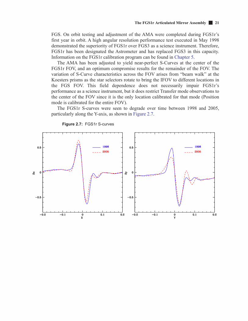
The FGS1r S-curves were seen to degrade over time between 1998 and 2005,particularly along the Y-axis, as shown in Figure 2.7.

Figure 2.7: FGS1r S-curves


However, since 2005 the S-curves changes were insignificant, as shown in Figure2.8

Figure 2.8: FGS1r S-curves 2005

Therefore, with the FGS1r demonstrating long term stability, the AMA wasadjusted once again on January 22, 2009 to restore the instrument's S-curves at thecenter of its FOV. It is important to note that Transfer mode science observationsobtained (before) after January 22, 2009 should use calibration data obtained (before)after that date for the scientific analysis of that data.

FGS Aperture and Filters 23

Figure 2.9: Shows the changes in the FGS1r S-curves resulting from the January 2009 AMA adjustment.

2.6 FGS Aperture and Filters

2.6.1 FOV and Detector CoordinatesFigure 1.2 shows the HST focal plane positions of the FGSs as projected onto the

sky. Figure 2.10 is similar, but includes the addition of two sets of axes: the FGSdetector coordinate axes, and the POSTARG coordinate axes (used in the Phase IIproposal instructions to express target offsets).

Each FGS FOV covers approximately 69 square arcmin, extending radially from10 arcmin to 14 arcmin from the HST’s boresight and axially 83.3 degrees on the innerarc and 85 on its outer arc. The IFOV determined by the star selector assemblies andfield stops is far smaller, covering only 5 x 5 arcsec. Its location within the pickledepends upon the Star Selector A and B rotation angles. To observe stars, the starselector assemblies must be rotated to bring the IFOV to the target. This procedure iscalled slewing the IFOV.

The detector reference frame and the POS TARG reference frames dif-fer from each other and from the Vehicle Coordinates V2,V3 (orU2,U3).


The (X,Y) location of the IFOV in the pickle is calculated from the Star SelectorEncoder Angles using calibrated transformation coefficients. Each FGS has its owndetector space coordinate system, the (X,Y)DET axes, as shown in Figure 2.10. FGS2and FGS3 are nominally oriented at 90 and 180 degrees with respect to FGS1r, butsmall angular deviations are present (accounted for in flight software control and datareduction processing). The FGS detector reference frame is used throughout thepipeline processing. The POS TARG coordinate axes, (X,Y)POS, should be used toexpress offsets to target positions in the Phase II proposal (Special Requirementscolumn). See Chapter 5: Writing a Phase II Proposal for more details.

The approximate U2,U3 coordinates for the aperture reference position (defaultplacement of a target) for each FGS and the angle from the +U3 axis to the +YDET and+YPOS Axis are given in Table 2.3. The angles are measured from +U3 to +Y in thedirection of +U2 (or counterclockwise in Figure 2.10). Note that the FGS internaldetector coordinate reference frame and the POS TARG reference frame have oppositeparities along their respective X-axes.

Table 2.3: Approximate Reference Positions of each FGS in the HST Focal Plane

Aperture U2(arcsec)

U3(arcsec)

Angle (from +U3 axis)

FGS1r –723 +10 ~270

FGS2r2 0 +729 ~0

FGS3 +726 +6 ~90

FGS Aperture and Filters 25

Figure 2.10: FGS Proposal System and Detector Coordinate Frames

2.6.2 Filters and Spectral CoverageFilter Bandpasses

The filter wheel preceding the dielectric beam splitter in each FGS contains five42mm diameter slots. Four of these slots house filters—F550W, F583W, F605W andF5ND—while the fifth slot houses the PUPIL stop. This stop helps restore theS-Curve morphology throughout the FOV of each FGS by blocking out the outer 1/3perimeter of the spherically aberrated primary mirror. The filter selection for eachFGS, their central wavelengths, and widths are listed in Table 2.4. The transmissioncurves (filters and PUPIL) are given in Figure 2.11. The PMT efficiency is given inFigure 2.12.

V3

V2U2

U3

XDET

YDET

YPOS

XPOS

XPOS

YPOS

YDET

XDET

XDET

YDET YPOS

XPOS

X,YDET = Detector Coordinate Frame in Object Space

X,YPOS = POS TARG Reference Frame Used in Phase II Proposal

FGS 3 FGS 1R

FGS 2R2


Figure 2.11: FGS1r Filter Transmission

Table 2.4: Available Filters

FilterCentral

WavelengthÅ

Spectral RangeÅ

FWHMÅ FGS

F583W 5830 4600–7000 2340 1,1R,2,3

F605W 6050 4800–7000 1900 1,1R,2

PUPIL 5830 4600–7000 2340 1,1R,2,3

F550W 5500 5100–5875 750 1,1R,2,3

F650W 6500 6200–6900 750 3

F5ND 5830 4600–7000 2340 1,1R,2,3

FGS Calibrations 27

Figure 2.12: PMT Efficiency

2.7 FGS CalibrationsFor the most part, the calibration requirements of the current Cycle’s GO science

programs will be supported by STScI. For Position mode observations, this includesthe optical field angle distortion (OFAD) calibration, cross-filter effects, lateral coloreffects, and the routine monitoring of the changes in distortion and scale across theFOV.

For Transfer mode, STScI will calibrate the interferograms (S-Curves) as afunction of a star’s spectral color. In addition, the S-Curves will be monitored fortemporal stability.

Only the center of the FGS1r FOV will be calibrated for Transfermode observations.

CHAPTER 3:

FGS Science GuideIn this chapter . . .

3.1 The Unique Capabilities of the FGSAs a science instrument the FGS offers unique capabilities not presently available

by other means in space or on the ground. Its unique design and ability to sample largeareas of the sky with milliarcescond (mas) accuracy or better gives the FGSadvantages over all current or planned interferometers.

The FGS has two observing modes, Position and Transfer mode. In Position modethe FGS measures the relative positions of luminous objects within its Field of View(FOV) with a per-observation accuracy of ~ 1 mas for targets with 3.0 < V < 16.8.Multi-epoch programs can achieve relative astrometric measurements with accuraciesapproaching to 0.2 mas.

In Transfer mode the FGS is used as a high angular resolution observer, able todetect structure on scales as small as 8 mas. It can measure the separation (with ~1mas accuracy), position angle, and the relative brightness of the components of abinary system down to ~10 mas for cases where V < 1.5. For systems with acomponent magnitude difference of 2.0 < m < 4.0, the resolution is limited to 20mas.

By using a “combined mode” observing strategy, employing both Position mode(for parallax, proper motion, and reflex motion) and Transfer mode (for determination

3.1 The Unique Capabilities of the FGS / 283.2 Position Mode: Precision Astrometry / 29

3.3 Transfer Mode: Binary Stars and Extended Objects / 293.4 Combining FGS Modes: Determining Stellar Masses / 34

3.5 Angular Diameters / 363.6 Relative Photometry / 36

3.7 Moving Target Observations / 383.8 Summary of FGS Performance / 38

3.9 Special Topics Bibliography / 39

28

Position Mode: Precision Astrometry 29

of a binary’s visual orbit and relative brightnesses of the components), it is possible toderive the total and fractional masses of a binary system, and thus the mass-luminosityrelationship for the components.

Alternatively, if a double lined spectroscopic system is resolvable by the FGS, thenthe combination of radial velocity data with Transfer mode observations can yield thesystem’s parallax and therefore the physical size of the orbit, along with the absolutemass and luminosity of each component.

In this chapter, we offer a brief discussion of some of the science topics mostconducive to investigation with the FGS.

3.2 Position Mode: Precision AstrometryA Position mode visit consists of sequentially measuring the positions of stars in

the FGS FOV while maintaining a fixed HST pointing. This is accomplished byslewing the FGS Instantaneous Field of View (IFOV, see Figure 1.3) from star to starin the reference field. acquiring each in FineLock (fringe tracking) for a short time (2to 100 sec.). This yields the relative positions of the observed stars to a precision of ~1milli-arcsecond (mas).

With only three epochs of observations at times of maximum parallax factor (a totalof six HST orbits), the FGS can measure an object’s relative parallax and propermotion with an accuracy of about 0.5 mas. Several multi-epoch observing programshave resulted in measurements accurate to ~0.2 mas. Unlike techniques which relyupon photometric centroids, the accuracy of FGS measurements are not degradedwhen observing variable stars or binary systems. And techniques which mustaccumulate data over several parallactic epochs would have greater difficultydetecting comparably high frequency reflex motions (if present).

3.3 Transfer Mode: Binary Stars and Extended ObjectsIn Transfer mode, the FGS scans its IFOV across a target to generate a time-tagged

(40 hz) mapping between the position of the IFOV (in both X and Y) and counts in thefour PMTs. These data are used to construct the interferogram, or transfer function, ofthe target via the relation

Sx = (Ax – Bx) / (Ax + Bx)

as described in Chapter 2. The data from multiple scans are cross correlated andco-added to obtain a high SNR transfer function.

In essence, Transfer mode observing is conceptually equivalent to sampling anobject’s PSF with milliarcsecond pixels. This enables the FGS to resolve structure onscales finer than HST’s diffraction limit, making it ideal for studying close binarysystems and/or extended objects.

30 Chapter 3: FGS Science Guide

The transfer function of a multiple star system is a normalized linear superpositionof the S-Curves of the individual stars, with each S-curve scaled and shifted by therelative brightness and angular separation of the components. If the components arewidely separated (> ~60 mas), two S-Curves are clearly observed in the transferfunction, as illustrated in the left panel of Figure 3.1. Smaller separations result inmerged S-Curves with modulation and morphology differing significantly from that ofa single star. Figure 4.3 illustrates these points.

By using point source S-curves from the calibration library one can deconvolve thecomposite observed transfer function of a binary star into component S-Curves (doneby either Fourier Transforms or semi-automated model fitting) to determine theseparation, position angle, and relative brightness of the components. If enoughepochs of data are available, the time-tagged position angles and angular separationscan be used to construct the apparent relative orbit, from which one can derive theparameters P, a, i, and which define the true relative orbit. Note that thesemi-major axis is an angular quantity; to convert it to a physical length, one mustknow the object’s distance (which can be obtained from parallax measurements).

3.3.1 Observing Binaries: The FGS vs. HST’s CamerasThe FGS, while capable of very-high angular resolution observations, is not an

“imaging” instrument like HST’s cameras. However, the ability to sample the S-curvewith milli-arcsecond resolution allows the FGS to resolve structure on scales too finefor the cameras. To illustrate, we present a comparison between binary observationswith HST’s Planetary Camera (PC) and with FGS1r in Figure 3.1. The image at left isa PC snapshot image of the Wolf-Rayet + OB binary WR 146 (Niemela et al. 1998).To the right is a simulated FGS1r “image” of this binary shown at the same scale. Withthe 0.042" pixels of the PC, the binary pair is clearly resolved. Based on point-spreadfunction (PSF) photometry, Niemela et al. publish a separation of 168 mas forthis pair. In comparison, an analysis of the FGS “observation” of the binary yields aseparation of 168 mas, a far more accurate result.

31

1

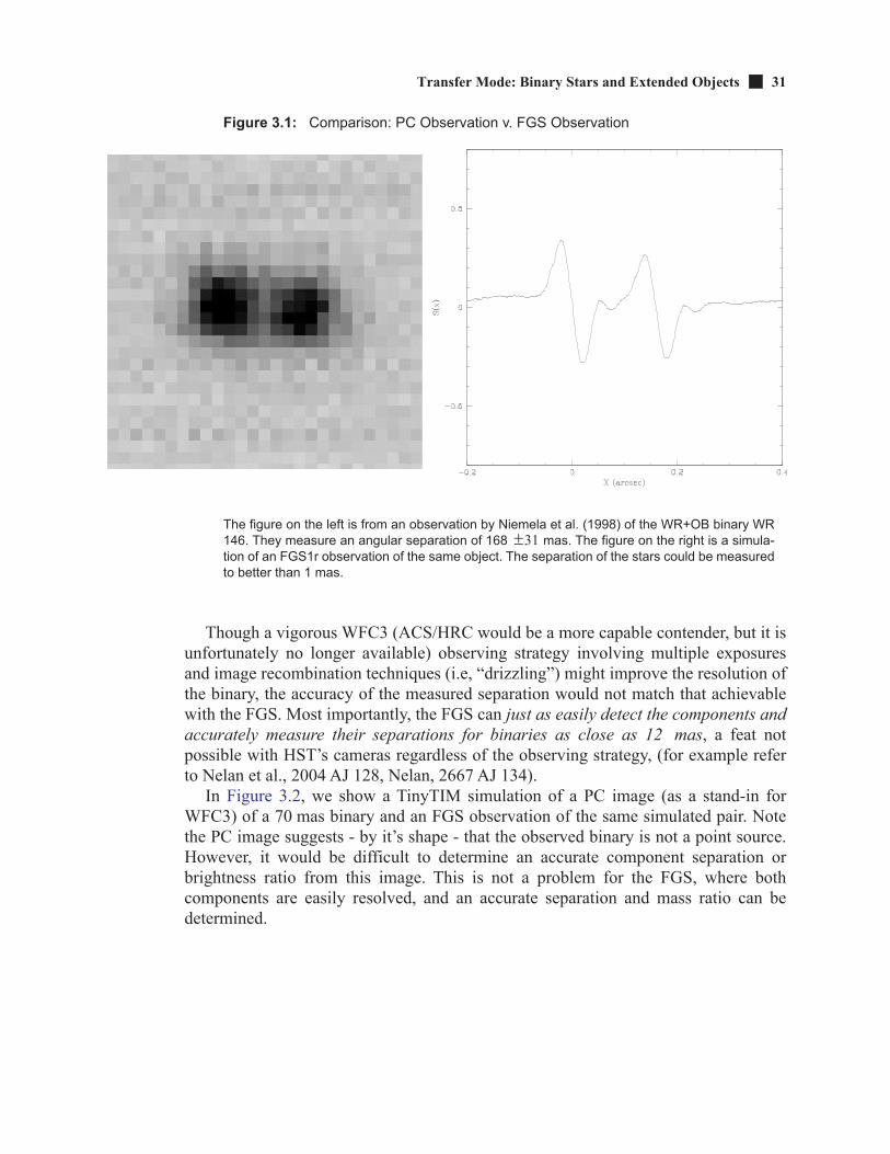
Transfer Mode: Binary Stars and Extended Objects 31

Figure 3.1: Comparison: PC Observation v. FGS Observation

The figure on the left is from an observation by Niemela et al. (1998) of the WR+OB binary WR146. They measure an angular separation of 168 mas. The figure on the right is a simula-tion of an FGS1r observation of the same object. The separation of the stars could be measuredto better than 1 mas.

Though a vigorous WFC3 (ACS/HRC would be a more capable contender, but it isunfortunately no longer available) observing strategy involving multiple exposuresand image recombination techniques (i.e, “drizzling”) might improve the resolution ofthe binary, the accuracy of the measured separation would not match that achievablewith the FGS. Most importantly, the FGS can just as easily detect the components andaccurately measure their separations for binaries as close as 12 mas, a feat notpossible with HST’s cameras regardless of the observing strategy, (for example referto Nelan et al., 2004 AJ 128, Nelan, 2667 AJ 134).

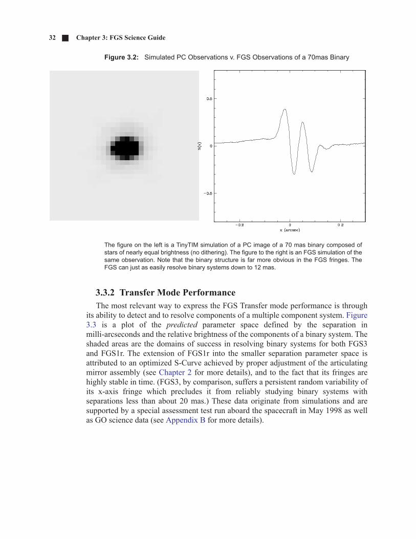
In Figure 3.2, we show a TinyTIM simulation of a PC image (as a stand-in forWFC3) of a 70 mas binary and an FGS observation of the same simulated pair. Notethe PC image suggests - by it’s shape - that the observed binary is not a point source.However, it would be difficult to determine an accurate component separation orbrightness ratio from this image. This is not a problem for the FGS, where bothcomponents are easily resolved, and an accurate separation and mass ratio can bedetermined.

31


Figure 3.2: Simulated PC Observations v. FGS Observations of a 70mas Binary

The figure on the left is a TinyTIM simulation of a PC image of a 70 mas binary composed ofstars of nearly equal brightness (no dithering). The figure to the right is an FGS simulation of thesame observation. Note that the binary structure is far more obvious in the FGS fringes. TheFGS can just as easily resolve binary systems down to 12 mas.

3.3.2 Transfer Mode PerformanceThe most relevant way to express the FGS Transfer mode performance is through

its ability to detect and to resolve components of a multiple component system. Figure3.3 is a plot of the predicted parameter space defined by the separation inmilli-arcseconds and the relative brightness of the components of a binary system. Theshaded areas are the domains of success in resolving binary systems for both FGS3and FGS1r. The extension of FGS1r into the smaller separation parameter space isattributed to an optimized S-Curve achieved by proper adjustment of the articulatingmirror assembly (see Chapter 2 for more details), and to the fact that its fringes arehighly stable in time. (FGS3, by comparison, suffers a persistent random variability ofits x-axis fringe which precludes it from reliably studying binary systems withseparations less than about 20 mas.) These data originate from simulations and aresupported by a special assessment test run aboard the spacecraft in May 1998 as wellas GO science data (see Appendix B for more details).

Transfer Mode: Binary Stars and Extended Objects 33

Figure 3.3: Comparison of FGS1r and FGS3 Transfer Mode Performance

Table 3.1 contains the expected resolution limits for FGS1r. Columns 1 and 2 showthe separation and accuracy for a single measurement, column 3 details the relativebrightness limit needed to achieve that precision, and the last column is the apparentmagnitude of the system. For example, a separation of 10 mas is detectable if thesystem is ~14 magnitudes or brighter and the magnitude difference of the components(m) is less than 1.0. Likewise, the separation of the components of a V=16.6 binaryis measurable to an accuracy of about 2 mas if their separation is greater than ~15 masand their magnitudes differ by less than 2.

Table 3.1: FGS1r TRANSFER Mode Performance: Binary Star

MinimumSeparation

(mas)

EstimatedAccuracy

(mas)MaximumMag Maximum V

7a

a. This represents detection of non-singularity under ideal condi-tions. Reliable measurements of the angular separation might not be achievable.

– 1.0 14.0

10a - 1.0 15.0

15 2 2.0 16.6

20 1 2.5 16.2

20 2 3.0 16.2

50 1 3.5 15.5

FGS1RFGS3

0

2

1

3

4

ΔM

agni

tude

20 30 50 1001086

Binary Separation (mas)


3.4 Combining FGS Modes: Determining Stellar MassesStellar mass determination is essential for many astronomical studies: star

formation, stellar evolution, calibrating the mass/luminosity function, determining theincidence of stellar duplicity, and the identification of the low-mass end of the mainsequence, for example.

The combination of Position mode and Transfer mode observations is an effectivemeans to derive a full orbital solution of a binary system. Wide-angle astrometry froma multi-epoch Position mode program can be used to measure the parallax, propermotion and reflex motion of a binary system. High angular resolution Transfer modeobservations can be used to determine the relative orbit and differential photometry ofthe components. Figure 3.4 illustrates the benefit of this technique as applied to thelow mass binary system Wolf 1062 (Benedict et al. 2001). The small inner orbit of theprimary star was determined from Position mode measurements of the primary’sposition relative to reference field stars. The large orbit of the secondary low masscompanion was derived from Transfer mode observations of the binary, which at eachepoch yields the system separation and position angle. Combining these data allowsone to locate the system barycenter and thereby compute the relative mass of eachcomponent. And with the parallax known (from the Position mode data), the totalsystem mass, and hence the mass of each component, can be determined.

Combining FGS Modes: Determining Stellar Masses 35

Figure 3.4: Relative Orbit of the Low-Mass Binary System Wolf 1062 AB

Figure 3.4 shows the orbits of the components of Wolf 1062 about the system’s barycenter. Thishas been determined from both Transfer mode observations, which yield the relative orbit, andPosition mode observations, which map the orbit of the primary relative to reference stars dis-tributed about the FGS FOV (in effect establishing the inertial reference frame). Note that thePosition mode data also yield the system’s parallax and proper motion.

0.2

0.1

0.0

-0.1D

eclin

atio

n (a

rcse

c)

-0.2 -0.1 0.0 0.1RA (arcsec)

0° (N)

90°(E)

12

3

45

6

8

9

1011

1214

15

1617

W 1062 ABM A 0.379 0.005 M SUN=M B 0.192 0.003 M SUN=

Figure courtesy of G. Fritz Benedict, University of Texas at Austin


3.5 Angular DiametersThe FGS has been used (Lattanzi et al. 1997) to determine the angular diameters of

non-point sources. The example given in Figure 3.5 shows the Transfer Function of aMira-type variable superposed on the S-Curve of a point source (both observed withFGS3). The extended source - a disk of 78 mas - is clearly distinguishable from apoint source. In addition to stellar discs, other objects which might be (or have been)resolved by the FGS include galactic nuclei, asteroids, and planetary moons.

Figure 3.5: Mira-type variable with a resolved circumstellar disk

3.6 Relative PhotometryWhile observing in Position mode, FGS3 serendipitously observed the outburst of a

flare on the nearby star Proxima Centauri (Figure 3.6, see Benedict et al. 1998). TheFGS has also been used to measure the relative flux of a star during an occultation ofthat star by the Neptunian moon Triton (Figure 3.7), and the data were subsequentlyused to examine the thermal structure of Triton’s atmosphere (see Elliot et al. 1998and Elliot et al. 2000).

The absolute FGS photometric response of FGS 3 has been stable at the 2% levelover the past eight years (L. Reed, BFGoodrich). FGS1r is expected to be as stable or

2

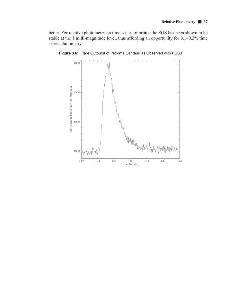
Relative Photometry 37

better. For relative photometry on time scales of orbits, the FGS has been shown to bestable at the 1 milli-magnitude level, thus affording an opportunity for 0.1–0.2% timeseries photometry.

Figure 3.6: Flare Outburst of Proxima Centauri as Observed with FGS3


Figure 3.7: Triton Occultation of the Star TR180 as Observed by FGS 3

3.7 Moving Target ObservationsThe FGS is suitable for the observation of solar system objects in both Position and

Transfer modes. The technique to acquire the data is not as straightforward as standardHST moving target observations, but in cases where the target is not moving toorapidly, the observation is certainly feasible. We note that the FGS has been used inprevious Cycles to observe Main Belt asteroids, both in Position mode and in Transfermode. More detail on moving target observations can be found in Chapter 4.

3.8 Summary of FGS PerformanceIn Position mode, the FGS offers capabilities not achievable by other HST

instrument or by the current generation of ground-based interferometers. Thesecapabilities include:

• a large field of view (69 arcmin2).

• large dynamic range.

Special Topics Bibliography 39

• a per-observation precision of ~ 1 mas for V < 16.8.

• multi-epoch astrometry accurate to ~ 0.2 mas.

Similarly, the FGS Transfer mode offers:

• 7 to 10 mas resolution down to V = 14.5, with wider separations observable to V = 16.8.

• the ability to determine relative separation and position angle of a binary sys-tem’s components, and hence the apparent relative orbit of the system.

Additionally, mixed-mode observations - employing both Position mode andTransfer mode - allow the user to combine parallax, proper motion, and relative orbitinformation to derive the true orbit of a multiple-star system and a determination ofstellar masses.

The FGS’s two observing modes make it possible for the instrument to resolvestructure in objects too faint for other interferometers and on scales too small for anyimaging device, while simultaneously measuring the distance to that object. It isanticipated the FGS will be the sole occupant of this niche until the arrival of the longbaseline interferometer in space, such as the Space Interferometry Mission (SIM),expected to launch in 2009.

3.9 Special Topics Bibliography

3.9.1 STScI General Publications• Rose, S., Hubble Space Telescope Phase II Proposal Instructions for Cycle

23, STScI, 2015.

• Smith, E., HST Data Handbook, Version 8.0. STScI, 2011.

3.9.2 Position Mode Observations• Benedict, G. F. et al., "Interferometric Astrometry of the Detached White

Dwarf - M Dwarf Binary Feige 24 Using HST Fine Guidance Sensor 3: White Dwarf Radius and Component Mass Estimates", 2000, AJ, 119, 2382.

• McArthur, B. E. et al., "Astrometry with Hubble Space Telescope Fine Guid-ance Sensor 3: The Parallax of the Cataclysmic Variable RW Triangulum", 1999, ApJ, 520, L59.

• Harrison, Thomas E. et al., "Hubble Space Telescope Fine Guidance Sensor Astrometric Parallaxes for Three Dwarf Novae: SS Aurigae, SS Cygni, and U Geminorum", 1999, ApJ, 515, L93.

http://www.stsci.edu/hst/HST_overview/documents/datahandbook/intro_cover.html

http://www.stsci.edu/ftp/documents/p2pi/p2pi.pdf

http://www.stsci.edu/ftp/documents/p2pi/p2pi.pdf


3.9.3 Transfer Mode Observations• Benedict, G.F. et al., “Precise Masses for Wolf 1062 AB from Hubble Space

Telescope Interferometric Astrometry and MCDonald Observatory Radial Velocities”, 2001, AJ, 121.1607.

• Henry, T. J. et al., "The Luminosity Relation at the End of the Main Sequence (0.08 - 0.20 M_solar)",1999, ApJ, 512, 864.

• Gies, D. R. et al., “The O-type Binary 15 Monocerotis Nears Periastron,” 1997, ApJ, 475, L49.

• Lattanzi, M.G., et al., “Interferometric Angular Diameters of Mira Variables with the Hubble Space Telescope”, 1997, ApJ, 485, 328.

• Nelan, E.P., “Resolving LB11146 with HST’s Fine Guidance Sensor 2007, AJ 134, 193N.

• Nelan, E.P. “Resolving DB Stars in the Carina Nebula with HST’s Fine Guid-ance Sensor, 2004, AJ 128, 323N.

• Simon, M., S.T. Holfeltz, and L.G. Taff, “Measurement of T Tauri Binaries Using the Hubble Space Telescope Fine Guidance Sensors”, 1996, ApJ, 469, 980.

3.9.4 Miscellaneous Observations• Elliot, J. L. et al., “Global Warming on Triton,” Nature, 393, 765, 1998.

3.9.5 Web ResourcesMany additional documents, including Instrument Science Reports and ST

Analysis Newsletters are available through the FGS Web page:http://www.stsci.edu/hst/fgs/


CHAPTER 4:

Observing with the FGSIn this chapter . . .

4.1 Position Mode Overview

4.1.1 The Position Mode VisitA Position mode visit yields measurements of the location of objects in the FGS’s

total field of view (FOV), and hence their relative angular positions. The objects areobserved sequentially according to the sequence of exposure lines in the proposal. Thetarget list of a typical Position mode visit consists of the science object(s) andreference stars used to define the local reference frame. A subset of the targets,referred to as check stars, should be observed several times during the course of thevisit to track any spurious motion of the FGS’s FOV on the plane of the sky (e.g.,thermally induced drift or OTA focus changes). The changes in the positions of thecheck stars are used to model the drift as a function of time so that its contaminatingeffect can be eliminated from the astrometry.

An FGS astrometry visit begins when the HST computer - the 486 - commands theStar Selector Servos to place the IFOV at the predicted location of the first starspecified in the visit (as per Phase II proposal). Control is transferred to the FineGuidance Electronics (FGE) microprocessor, which commands the FGS to acquireand track the target (Search, CoarseTrack, and FineLock). Later, at a specificspacecraft clock time, after the exposure time + overhead has expired, the 486 resumescontrol of the FGS, terminates the FineLock tracking of the object and slews the IFOVto the expected location of the next star in the sequence. This process repeats until the

4.1 Position Mode Overview / 414.2 Planning Position Mode Observations / 42

4.3 Position Mode Observing Strategies / 514.4 Transfer Mode Overview / 53

4.5 Planning a Transfer Mode Observation / 564.6 Transfer Mode Observing Strategies / 61

41

42 Chapter 4: Observing with the FGS

FGS has completed all exposures in the visit. The spacecraft’s pointing is held fixedon the sky under the control of the guiding FGSs for the entire visit unless otherwiseinstructed by the Phase II proposal. The status flags, photometry and instantaneouslocation of the IFOV is recorded every 25 msec (40 Hz).

4.1.2 The Position Mode ExposureDuring a Position mode exposure the object is tracked in FineLock (see Appendix

A). After the target is acquired by the Search and CoarseTrack procedures, FineLockbegins with a WalkDown, a series of steps of the IFOV toward the CoarseTrackphotocenter. At each step, the IFOV is held fixed for a period defined by FESTIME(Fine Error Signal averaging time) while the PMT data are integrated to compute theFine Error Signal (FES, the instantaneous value of the S-Curve) on each axis. Oncethe FES on both axes have exceeded a pre-set threshold, FineLock tracking begins.The star selectors are continuously adjusted after every FESTIME to re-position theIFOV in an attempt to zero out the FES during the next integration period. Theobjective is to present the Koesters prism a wavefront with zero tilt.

The defining parameters of an exposure are the target magnitude, the filter, theFESTIME and the exposure time. These topics are discussed in the following sections.

4.2 Planning Position Mode Observations

4.2.1 Target Selection CriteriaWhen targets are selected for FGS Position mode observations, several options and

requirements should be considered. These options are described below.

Brightness The bright limit for FGS1r is V = 8.0 without the neutral density filter in place.

With the F5ND filter, objects of V = 3.0 or fainter can be observed. The faint limit is V~ 17.0.

Near Neighbors FGS target acquisition in Position mode will be unreliable if the target has a

neighbor of comparable or greater brightness within a radius of 10 arcseconds. Inessence, the FGS’s IFOV - a 5" x 5" box - expects to encounter the target star withinthe search radius. Companions of similar brightness within this search radius may bemistakenly acquired instead of the target. However, for magnitude differences m > 1,companions within ~ 6" will not affect the acquisition of the brighter target. Note thatbinary stars with component separations less than about 0.5" can be successfullyacquired in Position mode, regardless of the m. Refer to the discussion under Section4.2.5 for further details regarding the acquisition of binary systems in Position mode.

Planning Position Mode Observations 43

Target FieldThe target field consists of the science target and reference stars. Observations of

the reference stars will be used to define the local reference frame for relativeastrometry. Since the optical field angle distortions are calibrated most accurately inthe central region of the FOV, the pointing of the spacecraft (via POS_TARGcommands - Chapter 6 for more details) should be specified to place the target field (asmuch as possible) in this area.

If the visit also includes Transfer mode observations of an object, the spacecraftpointing should be chosen to place the object at the FOV center, as this is the onlylocation calibrated for Transfer mode. If the target field geometry requires the Transfermode observations be executed at other locations in the FOV, special calibrations willbe needed. Proposers should consult STScI’s Help Desk for assistance.

Reference StarsIdeally, reference stars should have the following characteristics:

• Have magnitudes in the range 8 < V < 15 to avoid the need for an F5ND cross-filter calibration and to minimize exposure times.

• Be geometrically distributed around the target.

• Have at least 10 arcsec distance between one another and from the science tar-get to avoid acquisition of the wrong object.

• Should fall within the FOV for all HST orientations specified in the proposal.

Check StarsCheck stars, which are a subset of the target list, are observed several times over the

course of an orbit (visit). Two or more check stars, distributed across the field, providethe information needed to characterize the drift of the FGS’s FOV on the sky (which istypically about 4 mas over the course of the visit). Each check star should be observedat least three times. The best check stars are brighter than 14th magnitude to minimizeexposure time, and should include the science object for the highest accuracyastrometry.

4.2.2 FiltersTable 4.1 is a listing of the FGS1r filters, their calibration status and applicable

brightness restrictions. (Refer back to Figure 2.11 for the filter transmissions as afunction of wavelength.)


PUPIL Not Recommended for Position ModeOccupying the fifth slot on the wheel is the PUPIL. It is not a filter but rather a 2/3

pupil stop. Use of the PUPIL significantly reduces the degrading effect of sphericalaberration (which does not necessarily improve Position mode performance) butcollaterally alters the field dependence of the distortions. Consequently, the OFADcalibration for the F583W filter cannot be applied to PUPIL observations. In addition,PUPIL observing attenuates the object’s apparent brightness by nearly a fullmagnitude, which sets the faint limiting magnitude at about V=16 while makingobservations of stars fainter than V = 14.5 excessively time consuming.

FESTIME and Signal-to-NoisePhoton statistics dominates the noise in the measured position of stars fainter than

V ~ 13.0. To track fainter objects, the Fine Error Signal must be integrated for longerperiods. Table 4.1 lists the default FESTIMES for various target magnitudes. Thedefault FESTIMES, determined from the Phase II target magnitude, are appropriatefor most observations, and are set to ensure that photon noise, when converted into theNoise Equivalent Angle (NEA), does not exceed a predefined angular error threshold.The NEA is given by the relation

Table 4.1: Filters for which FGS1r will be Calibrated

Filter Calibration Status Comments Target Brightness

Restrictions

F583W Full “Clear” filter; OFAD calibration filter; Position Mode Stability Monitor

F5ND Limited Pos Mode Cross Filter calibration with F583W; limited to selected loca-tions within the FOV.

Required for targets w/3.0 < V < 8.0;

PUPIL No Not calibrated V > 7.5

F605W No Not calibrated V > 8.0

F550W No Not calibrated V > 7.5

Only the F583W filter will be calibrated for Position mode for the fullFGS FOV. Filter F5ND will be calibrated only at selected locationswithin the FOV

V 8.0

NEA 11.51 107------------------------- 0.5 C B+

0.5 C t ------------------------------.=


The NEA is used by the proposal processing tool (APT) to set the default FESTIMEtime. The parameter C is the total count rate expected from the target summed over allfour PMTs, B is the background count rate, and t is the FESTIME. The NEA is plottedas a function of magnitude and FESTIME in Figure 4.1. C as a function of filter andmagnitude for FGS1r is given by:

The constant f-factor is a function of the filter and the target’s spectral color. Table4.3 provides the f-factor for each combination of filter and color. The default FEStimes used by the proposal processing software for Position mode measurements arelisted in Table 4.1.

Table 4.2: Default FES Times

V Magnitude FESTIME(seconds)

8–12 0.025

13 0.050

14 0.1

15 0.4

16 1.6

17 3.2

C 20776 f-factor 10 0.4 V 13– –=


Figure 4.1: Default FESTIME as a Function of V Magnitude for F583W FGS1r: NEA as a Function of Magnitude and FESTIME

t = 0.025 sec

t = 0.050 sec

t = 0.100 sec

t = 0.400 se

c

t = 0.200 se

c

t = 0.800 se

c

t = 1.600 se

c

t = 3.

200 s

ec


Table 4.3: F-factor Transmission Estimator for Combination of Filter and Color

4.2.3 BackgroundBackground noise includes cosmic ray events, particle bombardment during

passages through the South Atlantic Anomaly (SAA), and scattered light falling in the5 x 5˝ IFOV. Cosmic ray events are suppressed by special circuitry and the FGS isprohibited from operating while transiting regions of heaviest impact from the SAA.Table 4.4 gives the typical dark + background counts for FGS1r in 0.025 seconds.Typically these values appear to be valid for all observations of isolated targets(suggesting that the dark counts dominate the background contribution). If thebackground counts for a specific observation are needed for the analysis of theobservation, such as when the source is embedded in significant nebulosity or in acrowded star field, it can be obtained from the photometry gathered during the slew ofthe IFOV to (or away from) the target position. These data extracted by the FGSpipeline package CALFGSA from the FITS files that input are cleaned of spikes from“interloping stars” and can be used to estimate the background levels duringpost-observation data reduction.

Table 4.4 lists the average dark+background counts/25 msec for each of the FGS1rPMTs. These data were serendipitously gathered over a 45 minute interval from afailed science observation (the target was not acquired due to a guide star problem).These data have proved invaluable for the analysis of Transfer mode observation offaint stars (V>15).

FilterB-V

+1.78 +0.60 +0.040 –0.24

F583W 1.000 1.000 1.000 1.000

PUPIL 0.491 0.491 0.491 0.491

F5ND 0.010 0.010 0.010 0.010

F550W 0.356 0.354 0.331 0.331

F605W 0.860 0.700 0.624 0.575


Table 4.4: FGS1r: Dark Counts

4.2.4 Position Mode Exposure Time CalculationsThe exposure time is the minimum time that an object will be tracked in FineLock.

Based the rate at which the measured location (or centroid) of a star converges (fromanalysis of FGS1r data) Table 4.5 lists the recommended exposure times as a functionof target magnitude. We note that:

• Exposures should be as short as possible to allow for more individual observa-tions during the visit, but should be longer than HST’s mid-frequency oscilla-tions (~10 seconds).

• Usually, Position mode observations yield an additional 10 to 20 seconds of FineLock data in excess of the exposure time specified in the phase2 proposal (a result of unused overheads). Hence, specifying a 10 second exposure results in 20 to 30 seconds of FineLock data.

4.2.5 Exposure Strategies for Special Cases Observing Binaries and Extended Sources in Position Mode

Multiple or extended sources in the FGS’s IFOV will result in a reduction of theamplitude of the observed interferometric fringes (relative to that of a point source).This occurs because light from multiple sources in the IFOV do not interact coherently(the observed rays originate from different angles on the sky). Therefore, multiplepoint source fringes will be superimposed upon one another, each scaled by therelative brightness of the source and shifted by its relative angular displacement on thesky. The result is a composite Transfer Function with reduced fringe visibility.

FGS1r PMTAverage

Background + DarkCounts per 0.025 sec

Ax 3.623

Ay 1.566

Bx 3.658

By 5.893

Table 4.5: Recommended FGS1r Exposure Times

Magnitude phase2 exposure time(in sec)

8–14 10

15-17 25


The fringe visibility reduction for the brighter component of a binary system withan angular separation along the X or Y axis greater than about 80 mas (i.e., when theindividual S-Curves are fully separate) is given by:

where fa and fb are the intensities of the brighter and fainter components, respectively.A similar expression, but with lb in the numerator, is appropriate for the faint starS-curve (see Figure 4.3 for examples).

For projected angular separations less that 80 mas, the Transfer Function will be ablend of the merged point source S-Curves. The resultant fringe visibility will dependon the relative brightness and the angular separation of the components (i.e., Fr ismore difficult to predict).

Even significant loss of fringe visibility does not pre-dispose the object from beingsuccessfully observed in Position mode. To be acquired in FineLock, an object’s FineError Signal (see Appendix A) must exceed a fringe detection threshold (see FigureA.2). The threshold is set on the basis of the target’s V magnitude, as entered in theproposal, to accommodate the acquisition of faint targets. (The fainter the target themore effectively the background and dark counts reduce the fringe amplitude, hencelower detection thresholds must be applied.) If the GO were to state the V magnitudeof a binary system or extended source to be sufficiently faint, (regardless of its truevalue), then the observed fringes will exceed the (lower) detection threshold, and theFGS will successfully acquire the object. However, if a false magnitude is specified,one should also manually set the FESTIME (an optional parameter) to the valueappropriate to the object’s true magnitude. Otherwise, the observation’s overheadswill be excessively long.

Some binary systems are not reliably observed in Position mode, even with theadjustment to the fringe detection threshold. Objects in this category include thosewith components exhibiting small magnitude differences (m < 1) and angularseparations greater than 60 mas but less than 800 mas (as projected along aninterferometric axis). In these cases, either star may be acquired. There have beencases where one component was acquired on the X-axis while the other was acquiredon the Y-axis. Such data are still useful, but care must be applied in the post-observation data processing.

There is a class of binary stars which cannot be observed in Position mode. In aFineLock acquisition (see Appendix A), the WalkDown to FineLock is a finite lengthpath (approximately 0.810") beginning at a point which is “backed off” a fixeddistance from the object’s photocenter. If the fringes of both stars lie outside this path,then neither will be encountered and the FineLock acquisition will fail. The condition

Frf a

f a f b+ -----------------------=


for such a failure is the following,

where X is the location of the system’s photocenter, ra and rb are the distances fromthe photocenter to the fringes of the components “a” and “b” respectively, la and lb arethe flux from each component, xs is the starting position of the WalkDown, and xl isthe length of the WalkDown. If the position of the binary along either the X or Y axisis known to meet this failure requirement, Position mode observations of this systemshould not be attempted.

It is recommended that a proposer contact the STScI Help Desk for assistance withPosition mode observations of binary systems.

4.2.6 Sources Against a Bright BackgroundFor sources against bright backgrounds, the fringe visibility function is reduced by

I / (I + B) where I is the point source flux and B is the background flux. The proposershould contact the STScI Help Desk for assistance with such observations.

4.2.7 Crowded Field SourcesCrowded fields create two problems for FGS observations:

• A nearby star (< 10 arcsec away) of similar magnitude could be acquired during the search phase.

• The background brightness in the 5 x 5 arcsec aperture may be increased by the presence of numerous faint stars or nebulosity.

The proposer should consult the STScI Help Desk for assistance with suchobservations.

Proposers should document—in the proposal—the logic for selectinga FESTIME or entering a false apparent magnitude of a target.

M MXra rb

xl ra > xl - la lb

rb > xsxs

xsra =la lb rb

Position Mode Observing Strategies 51

4.3 Position Mode Observing StrategiesMeasurement errors can be minimized by carefully structuring the order of

exposures in a visit. This section describes strategies which maximize science return.

4.3.1 Summary of Position Mode Error SourcesThe reduction of a Position mode data set requires several corrections and

calibrations:

• Exposure Level:

- Background determination.- Star Selector encoder positions (7 LSB).- PMT response.- Optical Field Angle Distortion calibration.- Differential velocity aberration.- Lateral color aberration.

• Visit Level:

- Vehicle jitter.- Drift of FGS’s FOV.- Cross filter (F583W v. F5ND, if used).

• Program Level:

- Plate solutions (4 or 6 parameter fits).- Plate scale.

Each of the corrections and calibrations are briefly discussed in Chapter 5, and arethoroughly reviewed in the FGS Data Handbook Many of the corrections specified onthe list are determined by analysis of individual observations and removed later in thedata reduction processing, (e.g., jitter data is retrieved from the guide star telemetryand removed from the target data). Calibrations, such as the plate scale, the OFAD,lateral color, and cross filter effect are derived from STScI calibration programs. Apotentially dominant source of error, the FOV drift (time scale of several minutes),must be measured during the visit, and to that end, the sequence of exposures must becarefully arranged.




4.3.2 Drift and Exposure SequencingStars observed more than once per visit (“check stars”) are typically seen to drift

across the FGS by ~ 2 to 6 mas when two FGSs guide the telescope (or ~ 5 to 20 maswith only one FGS guiding). Because astrometry observations execute sequentially,the errors in the measured angular separations between objects increase as the timebetween the measurements lengthens. If uncorrected, this drift will overwhelm theastrometry error budget.

Whatever causes the position of an object to “drift” in the astrometer’s FOV affectsthe guiding FGSs as well. The apparent motion of the guide stars are interpreted as“errors” by the pointing control system and are “corrected” by a small vehiclemaneuver. The astrometry FGS witnesses the pointing change. Therefore, the checkstar motion will have a contribution from all three FGSs.

When only one FGS is used for guiding, the telescope is not roll-constrained, andlarge motions in the astrometric FGS - up to 10 mas - are not uncommon.Nevertheless, this drift can be successfully removed from the astrometry data,provided the proposal specifies an adequate check star sequence. The more check starobservations, the more precise the drift correction. Check stars can be reference orscience targets. Ideally, both rotation and translation corrections should be applied tothe data, implying the use of at least two check stars with at least three measurementseach.

The need to observe check stars can be in conflict with other aspects defining anoptimal observing strategy, so compromises will be necessary. Overall an optimalPosition mode visit is scripted to:

• Define a check star strategy which will be robust against FOV drift.

• Maximize the number of reference stars observed.

• Maximize the number of observations of each object.

For example, a visit could contain 10–35 exposures, provided the overheads areminimized and exposure times are less than 20 seconds. A sample geometry is givenin Figure 4.2, where the science target is represented by the central object.

Figure 4.2: A Sample Visit Geometry

For the geometry specified above, the exposures may be sequenced as follows: 1 - 2 - target - 3 - 2 - 4 - target - 3 - 5 - 4 - target --> --> 2 - 1 - target - 3 - 5 - 4 - target - 2 - 1 - target.

Additional examples expressed in proposal logsheet syntax are given in Section 6.5.

35

42

1

Transfer Mode Overview 53

4.3.3 Cross Filter ObservationsTargets brighter than V = 8 cannot be observed with the F583W. The F5ND

attenuator must be used for such observations. If the visit includes observations offainter objects with the F583W, a cross-filter correction will be needed for the datareduction. For FGS3, the F583W/F5ND cross-filter effect was found to beastrometrically large (~ 7 mas) and varied with location in the FOV. This effect asbeen calibrated at the center of FGS1r’s FOV by STScI calibration programs. Ifneeded at other locations in the FOV, special calibrations by the proposer might berequired.

4.3.4 Moving Target Observation StrategyIn Position mode, the FGS can track a bright target (V ) whose motion is

less than ~ 0.1 arcsec per second. However, planning the observation requires extremeprecision: the moving target must be accurately located, to within 10 arcsec, in theIFOV at the start of the exposure, implying a very accurate ephemeris. Transfer modeobservations of moving targets are discussed in the next section.

4.4 Transfer Mode Overview

4.4.1 The FGS Response to a BinaryIf the source is a double star, then its wavefront has two components, each

incoherent with respect to the other. Two propagation vectors characterize thiswavefront and the angle between them is directly related to the angular separation ofthe stars on the sky. As the FGS’s IFOV scans across the object, each component ofthe wavefront can be thought of as generating its own interferogram (or “S-Curve”),whose modulation is diminished by the non-interfering “background” contributed bythe other component. The resulting relationship between the position of the IFOV tothe normalized difference of the PMTs depends on the separation of the stars and theirrelative brightnesses. The composite interferogram of a multiple system is the linearsuperposition of the fringes from the individual components, scaled by their relativebrightness and shifted with respect to one another by their separation on the sky.Given this, the fringe pattern of a binary system, whose components have an angularseparation (as projected along the X-axis) and fluxes fa and fb, is given by

14.0

Sbinary x l1S glesin x l2S glesin x + ,+=


where:

Figure 4.3 shows the changes in the observed FGS1r interferogram due to binarysystems of varied separations and magnitude differences. In Figure 4.3a we display theinterferogram of a wide binary pair with component separations and magnitudedifferences of (200 mas, 1.0) respectively. Figure 4.3b is an example of a system withthe same separation, but with a magnitude difference of m = 2.0. The binary systemin Figure 4.3c has a smaller separation and magnitude difference (50 mas and 0.5respectively), while in Figure 4.3d increases the magnitude difference to m = 2.0 fora component separation of 50 mas.

l1f a

f a f b+------------------- =

l2f b

f a f b+------------------- .=

Transfer Mode Overview 55

Figure 4.3: .Binary S-Curves Generated from FGS1r X-Axis Data

If the angular separation of the stars is greater than the width of the S-Curve, twodistinct S-Curves are apparent, but the modulation of each will be diminished relativeto that of a single star by an amount depending on the relative flux from each star (seeFigure 4.3a and also Figure 3.1). On the other hand, if the angular separation is small,the S-Curves will be superimposed, and the morphology of the resulting blendcomplicated (as in Figure 4.3d). In either case, the composite S-Curve can bedeconvolved using reference S-Curves from point sources, provided the angularseparations are not too small and the magnitude difference is not too large. To be moreprecise, fitting the observed double star S-Curve with two appropriately weighted,linearly superimposed reference S-Curves from single stars leads to the determinationof the angular separation, position angle, and magnitude difference of the binary’scomponents. The modulation, morphology, and temporal stability of the point-source

a b

c d


calibration S-Curves determine the resolving power of the FGS. For FGS1r, this isabout 7 mas for m < 1.0.

4.4.2 The Transfer Mode ExposureRather than tracking the fringe as in Position mode observation, the IFOV is

scanned across the object along a 45 degree path (with respect to the FGS detectoraxes) in a Transfer mode exposure. Every 25 milliseconds, star selector angles anddata from the four PMTs are recorded. From these data, the fringes of the object can bereconstructed. The number of scans and the length of each scan are derived from thePhase II proposal.

For each target, the step size and scan length must be adjusted as necessary toaccomplish the goals of the observation

• Step Size: The step-size refers to the angular distance covered by the IFOV along an axis during a 25 millisecond interval. The default step-size is 1.0 mas. Higher resolution is achievable using step sizes as fine as 0.3 mas. How-ever, such a small step size may prohibitively increase the total time to com-plete a scan, and as a result of least significant bit (LSB) constraints and vehicle jitter, the effective resolution may not be better than 1.0 mas. The goal is to execute as many scans as possible, with the smallest StepSize (0.6 or 1.0 mas), to achieve the highest S/N ratio.

• Scan Length: The required scan length is depends on the geometry of the tar-get. A minimum of scan length of 0.3" is needed to fully sample the fringes of a point source along with a sufficient segment of the wings to either side. For binary systems, the scan length should be at least as wide as the component separation plus 0.3".

4.5 Planning a Transfer Mode Observation

4.5.1 Target Selection CriteriaOther than the brightness restrictions specified in Table 4.6 there are several

additional considerations when selecting targets for Transfer mode observations.

The point-source calibration S-Curves are obtained only at the centerof the FGS1r FOV. Other locations in the FOV are not routinely cali-brated.

Planning a Transfer Mode Observation 57

• Position in the FOV: The morphology of the fringe varies considerably with position in the FOV, as shown for FGS1r in Figure 2.6. As explained in Chap-ter 2, this field dependence is the manifestation of small misalignment between the star selector optics and the Koesters prism which is greatly mag-nified by HST’s spherical aberration. To obtain the highest quality data with the best resolution, all Transfer mode observations should be obtained at the AMA optimized position at the center of the FOV. Under normal circum-stances, STScI will provide reference S-Curve calibrations only at the center of the Field of View.

• Color: The FGS’s interferometric response is moderately sensitive to the spectral color of the target. The FGS calibration library contains interfero-grams from point-source objects with a variety of (B-V) colors. The GO is encouraged to inspect this library to ascertain whether a suitable reference ((B-V) < 0.3) is available for data analysis. If not, the FGS group should be alerted, and efforts will be made to enhance the library. The color calibrations available in the FGS library are listed in Chapter 5. Up-to-date additions can be found on the FGS Web site:


• Minimum Scan Length: In order for Transfer mode observations to achieve the highest possible signal-to-noise, the length of the scan should be as short as possible (to allow for more scans in the allotted time). The minimum scan length is determined by the expected angular separation of the components of the binary being observed plus the recommended minimum size (for a point source) of 0.3", or,

where the value x is the largest anticipated angular separation of the binary along either axis.

• Maximum Scan Length: When considering the maximum scan length, three concerns should be addressed:

- Masking by the field stops becomes relevant when the FOV ismoved beyond 2 arcsec from the photocenter. False interferomet-ric features become prevalent.

- Beyond 2.5 arcsec from the photocenter, the intensity of the tar-get’s light drops off considerably, resulting in poor signal-to-noisephotometry.

- Maximum commandable scan length is 6.7".

• Target Orientation: If the approximate position angle of the non-point source is known, then specifying an orientation for the observation may be advanta-geous. If possible, (for wide binaries) avoid the situation where the projected angular separation along one of the axes is less than 20 mas. Specific orienta-tions are achieved by rolling the HST to an off-nominal roll attitude or by

Min Scan Length (arcsec) 0.7 2x,+=



scheduling an observation at a time when the nominal roll is suitable. It should be noted however that special orientations are considered as special schedul-ing requirements which affect schedulability.

• Target Field: The Search and CoarseTrack acquisition are vulnerable to acquiring the wrong object if the field is too crowded (with neighbors of com-parable brightness within 8 arcseconds of the target). Hence, the problem addressed in Section 4.2.7 for Position mode observations applies equally to Transfer mode observations.

4.5.2 Transfer Mode Filter and Color EffectsTable 4.6 is a summary of the available filters and associated restrictions governing

their use.

Table 4.6: FGS1r Transfer Mode Filters to be Calibrated During Cycle 8

The S-Curve morphology and modulation have a wavelength dependence.Experience with FGS3 has shown that the color of the reference star should be within(B – V) = 0.1 - 0.2 of the science target. We endeavor to maintain a library of singlereference stars which accommodate the color requirements of the GO proposals in theCycle. These color standards are usually observed once during the Cycle, whileUpgren69 is observed every 6 months to monitor S-curve stability.

4.5.3 Signal-to-Noise In essence, the “true” signal in a Transfer mode observation of a binary system is

the degree to which the observed Transfer Function differs from the S-curve of a pointsource. The signal-to-noise (S/N) required of an observation will depend upon theobject being observed; a wide binary whose stars have a small magnitude difference

FilterCalibration

Status at FOV Center

Comments Target Brightness Restrictions

F583W Full Monitoring of Reference Standard star Upgren69 and single epoch color calibra-tions as required by the GO proposal pool.

Recommended for V > 8.0;Not permitted for V < 8.0

F5ND Single-epoch color calibrations as

needed

Supported by the STScI Observatory Cali-bration program.

Required for V < 8.0; Not recommended for V > 8.0

PUPIL Single-epoch color calibrations as

needed

Not part of the STScI Observatory calibra-tion program. GO must request time from TAC for any calibrations.

Not permitted for V < 7.5

F605W Single-epoch color calibrations as

needed



F550W Single-epoch color calibrations as

needed



Planning a Transfer Mode Observation 59

and separation of 200 mas will be much easier to resolve than a pair with a largermagnitude difference and a separation of only 15 mas.

The “noise” in an observation has contributions from both statistical andsystematic sources. Photon noise, uncertainty of the background levels, and spacecraftjitter comprise the statistical component. The temporal variability and spectralresponse of the S-curves dominate the systematic component (these are monitoredand/or calibrated by STScI). Provided that at least 15 scans with a 1 mas step size areavailable, observations of bright stars (V < 13.0) suffer little from photon noise anduncertain background levels, and show only slight degradations from spacecraft jitter(with high S/N photometry, the segments of the data which are degraded by jitter areeasily identified and removed from further consideration).

Maximizing the S/N for observations of fainter objects requires a measurement ofthe background level (see Chapter 6) and a larger number of scans to suppress thePossonian noise in the photometry of the co-added product. But with lower S/Nphotometry in a given scan, corruption from spacecraft jitter becomes more difficult toidentify and eliminate. Therefore, the quality of Transfer mode observations of targetsfainter than V = 14.5 will become increasingly vulnerable to spacecraft jitter, nomatter how many scans are executed.

Systematic “noise” cannot be mitigated by adjusting the observation’s parameters(i.e., increasing the number of scans). To help evaluate the reliability of ameasurement made in Transfer mode, STScI monitors the temporal stability andspectral response (in B-V) of FGS1r’s interferograms. As discussed elsewhere, theFGS1r S-curves appear to be temporally stable to better than 1%, and the Cycle 10calibration plan calls for observations of single stars of appropriate B-V to support thedata reduction needs of the GOs (this calibration will be maintained in Cycle 26). Thisshould minimize the loss of sensitivity due to systematic effects.

4.5.4 Transfer Mode Exposure Time Calculations The step_size and number of scans determine the number of photometric

measurements available for co-addition at any given location along the scan path.Typically, up to 50 scans with 1mas step_size are possible within a 53 minuteobserving window, (after accounting for overheads and assuming a scan length~ 1.2 arcsec per axis). The step size and number of scans that should be specified arein part determined by the target’s magnitude and angular extent and also by the need toallocate time within the visit to any other objectives, such as Position modeobservations of reference stars (to derive a parallax for the binary). The total exposuretime for a Transfer mode observation (excluding overheads) is:

where Texp is the total exposure time in seconds, Nscans is the total number of scans,0.025 is the seconds per step, ScanLength is the length of the scan per axis in arcsec,and StepSize is given in arcsec.

T expScanLength

StepSize------------------------------- 0.025sec N scans =


Photon noise is reduced by increasing the number of scans, Nscans, as displayed inFigure 4.4, which demonstrates the benefits of binning and co-adding individualscans. Trade-offs between step size, length, and total duration of an exposure areunavoidable especially when considering visit-level effects such as HST jitter.

Figure 4.4: FGS1r (F583W) S-Curves: Single and Co-Added

Simulations using actual data scaled by target magnitude are needed to relate theTransfer Function signal-to-noise (described in the previous section) to the resolvingperformance of the instrument. A robust exposure time algorithm is in development.In Table 4.7, we offer some guidelines on the minimum number of scans to use in avisit for various binary parameters. These are derived for a step size = 1.0 mas, so thatin a 1 mas bin there would be NSCANS samples per bin. Smaller step sizes facilitatethe use of less scans to achieve the same signal-to-noise ratio. (Specificity fewer scanswith smaller step sizes can reduce the observational overhead, which can increase thetime on target and hence the overall signal-to-noise ratio. However, intermittentvehicle jitter may corrupt the data from some scans to the degree that such data isuseless for scientific purposes. These trade off need to be considered when planningthe observations).

Transfer Mode Observing Strategies 61

4.6 Transfer Mode Observing Strategies

4.6.1 Summary of Transfer Mode Error SourcesThe Transfer mode corrections and calibrations are:

• Exposure Level:

- Background subtraction.- Star Selector Encoder correction (7 LSB).- Cross-correlating and co-adding individual scans.- Availability of a suitable point-source reference S-Curve (color

response).

• Program Level:

- Roll dependence of the FGS plate scale.Each of the corrections and calibrations are discussed briefly in Chapter 5 and more

thoroughly in the FGS Data Handbook. Those corrections that could result in anenhanced observation strategy are discussed here.

Table 4.7: Suggested Minimum Number of Scans for Separations < 15 mas

V Mag mag =0.0 mag =1.5 mag =3.0

5 18 20 40

9 10 15 40

12 15 20 40

14 30 40 40

15 35 50 50

16 50 60a

a. Note that 60 scans is about the maximum that can be performed in a single HST orbit (assuming a scan length of ~1”). Multi-orbit visits do not necessarily increase the achievable S/N for targets of V>15 since photometric noise makes cross correlation of scans across orbital boundaries questionable. In other words, the data gathered during one orbit is not reliably combined with data from another orbit for faint, close binary systems.

60a




4.6.2 Drift CorrectionAs discussed in the Position mode section, targets observed multiple times per

Position mode visit typically drift across the FGS by about 6 to 12 mas when twoFGSs guide the telescope. This drift is also apparent in Transfer mode observations,but the cross-correlation of S-Curves prior to binning and co-adding automaticallyremoves the drift. Each single-scan S-Curve is shifted so that the particular features ofthe S-Curve used for the cross correlation coincides with that of the fiducial S-Curve.The reliability of implicitly removing the drift is only as good as the accuracy of thecross correlation procedure, which, for bright objects (V < 14.5) is accurate to < 1mas. Analysis is underway to determine the procedure’s accuracy for fainter objects.

4.6.3 Temporal Variability of the S-CurveMeasurements of the standard star Upgren69 over the lifetime of FGS3 indicated a

10 – 18% variability of the S-Curve morphology on orbital timescales. The amplitudeof these changes have important consequences on the analysis of binary starobservations when the separation of the components is less than 30 mas and themagnitude difference exceeds 1.6. These temporal changes also affect analyses ofextended source observations. The cause of this relatively high frequency variabilityin FGS3 has not been determined.

FGS1r appears to be stable at the 1% level over periods of many months to perhapsyears (as of July 2002). There appears to have been a slow evolution of the y-axisS-curve however, as shown in Figure 4.5. The changes along the X-axis have beenmuch less. On the assumption that this evolution is due to changes in the alignment ofthe interferometer with respect to HST’ OTA as water vapor outgasses from theinstrument’s graphite epoxy composites, it is expected that FGS1r will become morestable as time goes on (the rate of outgassing slows with time in orbit). STScI willcontinue to monitor FGS1r’s S-Curves so that this evolution can be calibrated and itseffect on science data minimized.

4.6.4 Background and Dark Counts SubtractionFor programs with isolated targets, background is not an issue. For programs with

targets embedded in nebulosity, knowledge of the background is required. In order toobtain a background measurement, it is necessary that there be at least two targets inthe observing sequence, separated by at least 60˝. The background will be measuredduring the slew of the IFOV from one target to the next. If necessary, the proposershould specify a false target at some location in the FOV at least 60˝ from the scienceobject, and observe it in Position mode for approximately 30 seconds with the samefilter as the science target. Care must be taken to avoid observing “background:objects brighter than V = 8.0 with F583W.

Dark counts become important for stars fainter than V=14.5. STScI has calibratedthe FGS1r dark counts. Therefore there is no need to acquire such data as part of ascience observing program. Likewise, the dead time correction is needed for stars

Transfer Mode Observing Strategies 63

brighter than about V=9, but STScI has already acquired the data needed to supportthis correction.

Figure 4.5: Evolution of S-curve morphology along the FGS1r Y-axis

4.6.5 Empirical Roll Angle DeterminationThe science data headers contain the commanded HST roll angle, not a measured

angle. The errors that contribute to a difference between the commanded and actualroll include: the relative guide star positional error, the FGS-FGS alignment error, anderrors in the predicted ephemeris. The actual roll angle is calculated from the guidestar telemetry by the observatory monitoring system, and is reported in the STScIObservation Logs that accompany the science data. More information is available onthe following Web page:

http://www.stsci.edu/hst/observatory/

The error in the calculated roll angle is estimated to be about 0.04 degrees. If amore accurate determination is needed, the position angle of the observed binary withrespect to the local reference frame can be measured via Position mode observationsof the target and a reference star (or two reference stars if the target cannot be acquiredin Position mode—see Section 4.2.5) should be included in the visit along with the

http://www.stsci.edu/hst/observatory


Transfer mode exposures. Please confer with STScI for help designing the visit andcalculating the roll from Position mode measurements.

4.6.6 Exposure Strategies for Special Cases: Moving TargetsFor Transfer mode observing, a moving target represents a special case. The flight

software which enables HST to track a moving target has not been implemented forFGS observations. Nonetheless, the FGS is quite capable of acquiring a moving targetprovided that the object’s angular speed is less than 80 mas/sec. However, during theobservation, the scan path is not adjusted to accommodate for the object’s motion. Thetarget’s fringe will be displaced in each subsequent scan until it moves completely outof the scan path. A method to work around this problem is to specify severalobservations of the object during the visit. For example:

1. The target should be observed in several short exposures rather than in one ortwo long exposures. The FGS would re-acquire the target with each newSearch, CoarseTrack acquisition regardless of the target’s motion. The targetlist should contain enough entries to cover the swath of sky traversed by themoving target, e.g., if the motion takes the object 10 arcsec across the FOV,then at least two sets of target coordinates should be specified.

2. The number of individual observations (entries in the exposure logsheet) andnumber of scans in an observation will be dictated by the object’s angularspeed.

3. Plan the observation when the target is moving its slowest, e.g., at opposition(if possible).

4. Take advantage of rolling the telescope to adjust the angle between the targetmotion vector and relevant FGS reference directions (please contact STScI forassistance).

5. Choose the exposure times to be as short as possible.

CHAPTER 5:

FGS CalibrationProgram

In this chapter . . .

5.1 Position Mode Calibrations and Error SourcesFGS science data is processed at three distinct levels: the exposure, the visit, and

the epoch. Each of these levels is subject to different sources of error. Table 5.1summarizes the accuracies of Position mode calibrations. Most of the errors listed arestatistical. Multi-epoch observations reduces the impact of these errors in the sciencedata.

5.1 Position Mode Calibrations and Error Sources / 655.2 Transfer Mode Calibrations and Error Sources / 73

5.3 Linking Transfer and Position Mode Observations / 795.4 Cycle 21 Calibration and Monitoring Program / 79

5.5 Special Calibrations / 80

65

66 Chapter 5: FGS Calibration Program

Exposure level calibrations address the per observation errors. The visit level correctionsaddress the errors after an entire orbit of astrometry data are combined The epoch-level correc-tions include the long term changes in scale and distortion of the instrument. The residuals aftercombining data from multiple visits include the plate overlays and, for example, the determina-tion of an object’s parallax and proper motion.

Table 5.1: FGS1r Position Mode Calibration and Error Source Summary

Type of Calibration Correction

Pre-Calibration Error Extent

Calibration Error(mas)

Comments

Exposure Level (per observation) Calibration Corrections:

background and detector dark counts

– – Addressed by increasing the integration time for each centroid determination when observ-ing faint stars. (to preserve the NEA).

Star Selector Encoder fine bit errors

~1 mas 0.1 Correction applied in the SSA,B->X,Y con-version.

Centroid errors Magnitude Dependent ~ 1, V < 15~ 2, V >15

Apply median filter.

Relative PMT sensitivity –~4 mas (V>15) 0.1 mas Analysis removes PMT mismatch effect; used to adjust for position centroid errors.

Differential velocity aber-ration

30 mas(function of geometry)

0.1 Depends on HST velocity vector and target geometry, ephemeris errors

Relative distortion across FOV (OFAD)

~ 500 mas ~0.3 mas STScI calibration in filter F583W.

Lateral color correction ~1 mas relative shift for B-V) = 1

0.1 mas STScI standard yearly calibration at center of FOV.

Cross filter calibration ~7 mas < 0.2 center Relative positional shifts are calibrated for fil-ters F583W and F5ND at FOV center.

Visit Level Calibration Corrections:

HST jitter 2–4 mas: quiet; 10–150 mas: extreme

incidents

< 0.1 during quiescence.

Correction derived from guide star motion. Large jitter excursions could cause loss of lock or corrupt a data set; disqualify outliers.

Drift 5–20 mas: two GS FineLock.

12–60 mas: one GS + gyro roll control

< 0.2 Special observing strategy for check stars; Drift models derived from check star motion and applied to target data.

Epoch-Level Calibration Corrections:

Temporal evolution of OFAD and plate scale.

<100> mas/year 0.2 mas Long-term stability monitor program: update OFAD coefficients and FGS star selector cali-bration.

Position Mode Calibrations and Error Sources 67

5.1.1 Position Mode Exposure Level CalibrationsThe corrections and calibrations described below are applied by the FGS

Calibration Pipeline.

Star Selector Encoder Fine Bit ErrorsThe star selector rotation angles are read as 21 bit integers. The 7 least significant

bits (LSBs) are read by an optical resolving device that was calibrated during themanufacturing process. The size of the calibrated correction is about 1 mas with aresidual of about 0.1 mas. Errors in the 14 most significant bits (MSBs) are absorbedby the OFAD calibration.

Position Centroiding The location of a star in the FOV during a Position mode observation is determined

by identifying the median of the 40 Hz SSA or SSB samples (while the target is beingtracked in FineLock). The median measurement is robust against most spacecraftjitter, short-interval transients and telemetry dropouts. If faint targets (V > 16.0) areobserved, the photometric noise results in a large noise equivalent angle. Spacecraftjitter and photometric noise contribute to the standard deviations about the median ofup to 2 mas per axis for V < 14.5 and up to 3 mas per axis for V > 15.0. However, therepeatability of the centroid measurement (over smaller intervals of the exposure) isthe true assessment of the precision of the measurement, typically 0.7 mas and 1.5 masfor targets where V < 14.5 and V > 15.0 respectively.

PMT Sensitivities and Position Centroid AdjustmentThe effect of PMT sensitivity on FGS observations is discussed in Appendix A. In

order to accommodate the differences between the two PMTs along each axis, theFGE computes an average difference (DIFF) and average sum (SUM) of theirphotometric response to the star over the first few FESTIMES in the WalkDown.These values are used in the calculation of the Fine Error Signal. The results areaccurate for bright (V < 14.0) objects but become unreliable for fainter targets, a resultof the short integration period and increasingly noisy photon statistics. The pipelinegathers photometric data over the entire WalkDown (typically 80 times as manysamples) to achieve a better signal-to-noise and more reliable values of DIFF andSUM. These are used to recompute the Fine Error Signal and adjust the (x,y) centroidsin post-observation data reduction.

Differential Velocity AberrationDifferential velocity aberration arises as a result of small differences in the angle

defined by the HST velocity vector and the line of sight to targets in the FGS FOV.The HST PCS guides for zero differential velocity aberration (DVA) at one position inthe FOV. The positions of targets elsewhere in the FOV must be corrected for DVA.Calibration errors in the relative alignment of the FGSs, catalog position errors of theguide stars, and ephemeris errors all contribute—though negligibly—to the errors inthe differential velocity aberration correction. The actual adjustment to the target’spositions can be as large as 30 mas (depending on the target and velocity vector


geometry) but are corrected by post-observation data processing to an accuracy of0.1 mas.

Optical Field Angle Distortion (OFAD) CalibrationField angle distortion introduces errors in the measurement of the relative angular

separation of stars at varied positions across the FGS FOV. The distortion errorsoriginate from:

• Radial distortions induced by the Ritchey-Chretian design of the OTA.

• Manufacturing irregularities in the FGS/OTA optical train.

• The optical reader produces errors in the 14 most significant bits of the 21-bit Star Selector A and B encoder values.

The distortion is independent of target magnitude, color, or exposure time, anddepends only on the location of the object in the FGS FOV. The Space TelescopeAstrometry Science Team (STAT) has calibrated the optical field angle distortion(OFAD) in FGS3 and maintained this calibration (the OFAD has a slow timedependence).

The data for calibrating FGS1r became available in December 2000. The analysis(by the STAT) was completed in June 2001. The distortion, on average about 500 masacross the FOV, is represented by two fifth-degree two-dimensional polynomials.Post-calibration residual errors are typically ~0.3 mas throughout most of the FOV.The OFAD calibration of FGS1r was part of the FGS1r commissioning calibrationplan.

The OFAD residuals for FGS1r are smaller than those of FGS3 due to the design ofthe calibration test. The FGS3 data were acquired at a time when the roll of HST wasrestricted to be within 30 degrees of nominal for the date of the observations. TheFGS1r test executed when the target field (M35) was close to the “anti-sun” position,i.e., when HST could be rolled over a full 360 degrees. Figure 5.1 shows an overlay ofthe pointings used for the FGS3 calibration, while Figure 5.2 shows the same for theFGS1r calibration. The freedom to rotate the field of view maximized the apparenteffect of the distortions, making them more easily measured compared to the FGS3test.

The accuracy of the astrometric catalog generated from ground based observationsis insufficient for calibrating an FGS as a science instrument. As part of the OFADcalibration, it was necessary to derive an accurate star catalog. This requires thatselected stars be observed at several HST pointings. In Figure 5.1 and Figure 5.2, thebold symbols denote stars that were observed as part of the calibration. For the FGS1rcalibration, special care was taken to maximize the number of pointings whichmeasured every star.


Figure 5.1: Overlay of the pointings used for the FGS3 OFAD calibration

Figure 5.2: Overlay of pointings used for the FGS1r OFAD calibration


Lateral ColorThe five-element corrector group (see box in Figure 2.1) is a collection of

refractive elements tasked with the removal of astigmatism and the final collimationof the beam. It’s refractive properties introduce subtle changes to angle of propagationof the beam as a function of the spectral color of the source. This change causes theapparent position of the star in the FOV to shift slightly, an effect referred to as lateralcolor. The positional error introduced by lateral color is relevant when comparing therelative positions of two targets of extreme colors: for example, a color difference of(B – V) = 1 between two targets could introduce a mas positional shift. An in-orbitassessment of lateral color associated with FGS1r was performed in December 2000and again in December 2001 (and will be repeated in December 2002). A dedicated onorbit calibration of the lateral color shift in FGS1r was first performed in December2000. A field of stars containing a blue star (A0) and a red star (M3) was observed atthree HST roll angles that differed by about 60 degrees (the field was near anti-sun, soHST roll angle was unconstrained). The three-orbit test was repeated in December2001. Since then the lateral color calibration has been monitored every two years. Theresults of these tests are available from the FGS Web site at:


5.1.2 Position Mode Visit Level CalibrationsJitter

Significant enhancements to the HST pointing control system and the replacementof the original solar arrays have reduced quiescent vehicular jitter to 2–4 mas.Although small for most HST science applications, the jitter must be removed fromastrometry data.

Since astrometric measurements are made sequentially, relating the measurementsto one another requires a mapping of each measurement onto a fixed commonreference that defines the visit. Guide star positional data, also telemetered at 40 Hz,are used to define jitter characteristics over the course of the visit. Using the timedependent guide star centroids, low frequency jitter (on time scales of minutes) can beremoved from the target data.

The pre-SM3B solar panels caused high frequency, large-excursion jitter, as HSTtransitioned to and from orbital day and night. These disturbances ranged in amplitudefrom 50 to 150 mas and lasted up to several tens of seconds. If particularly frenzied, atemporary or total loss of lock of the guide stars would result. An example of the jitterduring the onset of a day/night transition is shown in Figure 5.3. The large vibrationsincrease the standard deviations of FineLock tracking in the three FGSs by up to afactor of eight over the pre-transition values. Fortunately, such instances were rare.

With the new solar arrays installed during SM3B, the day/night disturbances nolonger cause significant vehicle jitter. With the new arrays, HST jitter is characterizedby two low amplitude (~5 mas) vibrational modes at 0.5 and 1.2 Hz. A larger,intermittent (and infrequent) disturbance of up to 100 mas persists, however.



Fortunately HST’s pointing control law damps this jitter away in about 10 seconds orless.

The overall residual from the “de-jittering” process is only ~ 0.1 mas, the smallvalue testifying to the advantages of using a median filter in the centroid computationand to the excellent tracking of guide stars by the guider FGSs.

Figure 5.3: FGS2 Guide Star Motion at the Onset of a Day/Night Transition

This plot shows the relative position of a guide star in FGS2 along the HST V3 axis as a functionof time. The large disturbance at about 157 seconds occurred as HST transitioned from orbitnight into daylight. This was typical until the new solar panels were installed in March 2002(SM3B). Significant jitter is no longer present at day/night or night/day transitions.

DriftFGS drift was discussed in Chapter 7 with regards to observation strategy, i.e., the

use of check stars to track apparent motion of the FOV during the visit so it can beremoved during post-observation processing. There are two different classes of drift,depending on whether one or two FGSs guided the HST during the visit. With twoFGSs guiding, drift is identified as a slow but correlated wander of the targetsobserved more than once during the visit. The amount of drift appears to be related tothe intensity of the bright Earth entering the telescope during target occultations.Accordingly, the drift is highest for targets in HST’s orbital plane (~ 10 mas) andlowest for those at high inclination (~ 2 mas).

When only one FGS is used to guide the telescope, the drift is typically 20 mas overthe course of the visit. The single guide star controls the translational motion of thespacecraft while the HST roll axis is constrained by the gyros. Gyro-induced drift

Samples every 0.025 s

Night to Day

Time (seconds)

V3

Poin

ting

(in a

rcse

c)


around the dominant guide star ranges from 0.5 to 5 mas/sec, and is typically of order1 mas/sec. Note the gyro drift is a spacecraft roll, and does not represent thetranslational motion of a target at the FGS (which will typically be ~0.01mas/sec).Over the course of a visit, the roll drift error measured by the astrometer can build upto 40 mas or more (but is typically less than 20 mas).

Regardless of the size of the drift, it can be characterized and removed by applyinga model to the check star motions, provided the visit includes a robust check starstrategy: a check star observation every 5–6 minutes (described in Chapter 7). At aminimum, two check stars measured three times each are needed to modeltranslational and rotational drift.

Cross Filter CalibrationsFor a target star (or any reference stars) brighter than V = 8.0 to be included as part

of an FGS observation, it must be observed with the neutral density attenuator F5ND.As a result of the differing thicknesses of F583W and F5ND, and possibly a wedgeeffect between the two filters, the measured position of the bright target in the FOVwill shift relative to the (fainter) reference stars. A cross-filter calibration is required torelate these observations, as relative positional shifts may be as high as 7 mas. Also,further evidence from FGS3 indicates these shifts are field dependent. If the effect isuncorrected, a false parallax will occur between the science and reference targets asthe star field is observed at different orientations in the FOV. Since it would beprohibitive to calibrate the cross-filter effect as a function of field location, FGS1rcross-filter calibrations will be restricted to the center of the FOV. For reference, theuncertainty after the FGS3 cross-filter calibration is ~0.5 mas.

5.1.3 Position Mode Epoch-Level CalibrationsPlate Scale and Relative Distortion Stability

For FGS3, the plate scale and OFAD exhibits a temporal dependence on an averagetime scale of ~4 months and a size of several tens of milli arcseconds (predominately,a scale change). The evolution of the FGS3 OFAD revealed that the variability isprobably due to the slow but continued outgassing (even after 10 years!) of thegraphite epoxy structures in the FGS. A long-term stability monitoring test is executedbi-monthly to help measure and characterize the distortion and relative plate scalechanges and thus update the OFAD. Post-calibration residuals are on average 1 masalong the X-axis and Y-axis. Better performance (of order 0.5 mas) is achieved inthe central region of the FOV.

The FGS1r Position mode stability was coarsely monitored during Cycle 7. Largescale changes in its S-Curve, attributed to outgassing effects, show that the instrumentwas unstable (for high accuracy astrometry) during its first year in orbit, as expected.In early 1998 the evolution slowed, and by April 1998 FGS1r’s S-curves fullystabilized; a major prerequisite for the OFAD calibration was met.

The OFAD and lateral color calibrations were to have been performed during cycle8 when the target field was at anti-sun and HST would not be roll constrained.Unfortunately this coincided with and was preempted by the Servicing Mission 3a.

Transfer Mode Calibrations and Error Sources 73

Rather than perform the calibrations under less favorable, roll-constrained conditions,STScI decided to defer the observations until December 2000, when the target fieldagain has an anti-sun alignment. The analysis of the OFAD data were carried out as a“calibration out sourced” proposal led by members of the STAT from the University ofTexas at Austin. The results of this calibration have been made available to STScI andreside as reference files used by the FGS calibration pipeline.

The science data that has accumulated since the beginning of cycle 8 can be fullycalibrated with the OFAD calibration. Any temporal evolution since the beginning ofcycle 8 is back-calibrated away by use of the long term monitoring observations thathave been executing all along. Check the FGS Web pages for updates with regard tothe OFAD calibrations.

Errors Associated with Plate OverlaysThe errors associated with several of the corrections described above will not

manifest themselves until data from individual visits are compared. The mostdominant source of Position mode error are the OFAD and changes in the plate-scale.The derivation of a plate scale solution is described in the FGS Data Handbook. Ingeneral, for regions near the center of the pickle, residuals are smaller than 1 mas if thereference star field is adequately populated.

5.2 Transfer Mode Calibrations and Error SourcesTable 5.2 summarizes Transfer mode sources of error and associated calibrations.

Each entry is described in the subsections below.A Transfer mode observation contains multiple scans of a target. To obtain optimal

S/N values, the individual scans are cross-correlated, binned, and co-added. Thereliability of this process is dominated by spacecraft jitter for targets with V < 14.5,and by photometric noise for fainter targets.

Background and Dark SubtractionTargets fainter than V ~ 14.5 are increasingly affected by dark counts which

reduces the amplitude of the S-Curve (since these contributions are not coherent withthe light from the star. see Chapter 7). The instrumental dark counts have beenmeasured as part of the STScI FGS calibration program (and are listed in Table 2.1).





These values are needed for the analysis of data from Transfer mode observations ofstars with V>14.

PMT Sensitivity DifferencesAlthough individual PMT sensitivities in an FGS differ, these differences do not

introduce a significant source of error in Transfer mode observations. Differences inthe PMT response manifest themselves as a bias (offset) of the S-Curve. This bias ispresent in the calibration standard star S-Curves (the single stars) as well, and so theeffect is neutralized when deconvolving the science target Transfer Function into itscomponent single S-Curves (provided the spectral colors of the science and referencetargets are well matched).

JitterTypically, quiescent vehicular jitter is about 2–4 mas in amplitude on timescales of

minutes. With the solar panels installed in March 2002 during SM3B, the large 150mas amplitude disturbances associated with the day/night orbital transitions of HSTdo not occur. Spacecraft jitter is removed by using the guide star centroids forquiescent times, or by eliminating intolerably corrupted scans or segments of scansfrom the co-addition process. For illustration, Figure 5.4 shows the effects of jitter onthe FGS1r interferogram (single scan).

Table 5.2: FGS1r Transfer Mode Calibrations and Error-Source Summary

Correction Pre-Calibration Error Extent

Calibration Error(mas)

Comments

Background and detector noise – – For bright backgrounds, use data serendipi-tously acquired during the FGS servo slew to the target. For dark measurements, use STScI calibration data.

HST jitter 2–4 mas: quiet;50–150: extreme

< 0.1 during quiescence

Use guide star data to remove HST jitter. Highly corrupted scans are deleted.

Drift 5–20 mas: 2 guide star FineLock.

12–60: 1 guide star plus gyro roll control

< 0.5 Cross correlation of S-Curve scans during post observation data processing removes drift errors.

S-Curve temporal variability ~1% in FGS1r limitsresolution

Monitor standard star (Upgren69).

S-Curve color dependence ~2% limitsresolution

Use calibration point source (i.e., an unre-solved star) of appropriate (B-V) color.


Figure 5.4: Effects of Jitter on an FGS1r S-Curve (single scan)

The quiescent scan (Figure 5.4a) shows features due to jitter - like the jump in S(y) around 0.03arcsecond - which can be filtered out during post-observation processing. Unfortunately, theextreme effects of vehicle jitter on the S-Curve shown in Figure 5.4b cannot be corrected. Scanssuch as this are deleted from further consideration in the analysis. Note the small variations inthe S-Curve’s wings seen near the extreme edges of the plot (i.e., +/- 0.08") are due to photo-metric noise (the data presented in this example are from an observation of a bright V=9 star).

DriftDrift is defined in Chapter 7, and its application to Position mode observations has

been discussed earlier in this chapter. Drift is also apparent in Transfer modeobservations but its removal from the raw data is straightforward; the cross-correlationof S-Curves, prior to binning and co-adding, automatically accounts for drift. Eachindividual S-Curve is shifted so that the particular feature of the S-Curve used for thecross correlation coincides with that of the fiducial S-Curve. However, the reliabilityof implicitly removing the drift is only as good as the accuracy of the cross correlationprocedure, which becomes photon noise dominated for stars fainter than V=15 (i.e.,cross correlation of scans is not reliable for V>15, hence drift can not be removedfrom such observations).

For bright stars with V < 13, FGS drift is estimated to degrade the resolution ofTransfer mode observations by about 0.5 mas. For fainter stars, the degradation isworse. If an observation of a faint star (V > 15) was subject to typical drift(10 to 12 mas), then the estimated loss of angular resolution would be ~ 3 mas.

a

b


Instrumental StabilityAnalysis of observations of resolved objects (i.e, binary systems or extended

sources) involves the de-convolution of the observed transfer function using referenceS-Curves of point sources. The repeatability, or temporal stability, of point-sourceS-Curves has a direct effect on the reliability (or accuracy) of the scientific result.FGS3 continued to demonstrate a variability of ~ 15% in its X-axis S-Curve (asdetermined from repeated observations of a standard star). This effectively renderedFGS3 unreliable for observing close (separations < 20 mas) binary systems. However,FGS1r has demonstrated repeatability at the 2% level, implying reliable measurementsof binary systems down to 7 mas.

Figure 5.5 illustrates FGS3’s persistent variability and FGS1r’s stability overcomparable timescales. Figure 5.5a shows FGS3’s inherent variability in the S-Curvesof the same point source over a 102-day span in 1997. Note this intrinsic variability inthe instrument is indistinguishable from its interferometric response to a 15 masbinary with m = 0.5 mag (when compared with a point-source, as shown in Figure5.5c). In contrast, the stability of FGS1r (Figure 5.5b) easily permits detection of the15 mas binary system (Figure 5.5d) when compared to a point-source. We note the“difference” seen in Figure 5.5d are due to systematic changes in the observedinterferogram (i.e., the object is resolved), not random effects.

As was discussed in Chapter 4, FGS1r has shown a slow “evolution” of its y-axisS-curve. This should not compromise the reliability of this instrument for observingclose binary systems; STScI will continue to observe calibration standards in eachcycle as needed so that GOs have access to calibration data appropriate of a givenepoch.

Interferometric Response and Source ColorThe morphology and amplitude of the S-Curve is sensitive to the spectral color of

the source. The point-source reference S-Curve used for comparison to the observedfringes of a science target should match the color of the target to within (B - V) = 0.3,especially when analyzing observations of close binaries (separations < ~40 mas). Thepoint source standards observed by FGS1r as part of the yearly observatory calibrationplans are chosen to meet the needs of the cycle’s GO science program. This includesconsideration of both the science target colors as well as the filter (F583W or F5ND)to be used by the GOs. For example, the cycle 10 FGS1r reference star color library isgiven in the Table 5.3.


Figure 5.5: Temporal Stability: FGS3 v. FGS1r

The two plots at the top compare the fringes of FGS3 (left) and FGS1r (right) from observationsof point sources taken at two different times. Clearly FGS3 shows significantly more variabilitythan FGS1r. The plots in the bottom row compare the FGS3 and FGS1r fringes of a point sourceto that of a 15 mas binary. Given FGS3’s temporal variability (top left plot), the detection of thebinary (bottom left plot) is questionable, unlike the reliable detection by FGS1r.

a b

c d


Table 5.3: Library of cycle 10 calibration point source S-curves

Transfer Mode Scale as a Function of HST Roll AngleTesting of FGS1r during its commissioning in Cycle 7 revealed that the measured

separation and position angle of the stars in a binary system is sensitive to the system’sorientation relative to the interferometer axis and hence the HST roll angle. Over time,as a system is observed at a variety of HST roll angles, this introduces systematicerrors into the derivation of the binary’s apparent orbit. The error in the measuredseparation of the stars can be as large as ~ 1% of the true projected separations, someasurements of wide binaries are affected more than those of close systems. Theeffect is believed to be due to a small rotation error of the Koesters prism(s) about thenormal to its entrance face.

During Cycle 9 a wide binary (KUI 83, component separation ~0.3”) was observedwith FGS1r in Transfer mode at three different HST roll angles (V3roll = 25, 43, 60degrees). The measured total separation of the components was constant to about 1mas, indicating that the scale is not dependent upon vehicle roll, in contradiction to theCycle 7 results. STScI will monitor this aspect of FGS1r’s performance, but at a lowfrequency (approximately every 2 to 3 years).

The point-source calibration S-Curves are obtained only at the centerof the FGS1r FOV. Other locations in the FOV are not routinely cali-brated.

Star R.A. Declination V mag B-V Filter

WD0148+476 01 52 02.9 +47 00 06 12.5 0.0 F583W

Latcol-B 05 59 27.3 +22 34 39 10.5 0.2 F583W

Upgren69 00 42 42.2 +85 14 14 9.6 0.5 F583W

HD 233877 11 52 54.1 +49 23 46 9.7 1.1 F583W

SAO185689 17 45 06.9 -29 08 37 9.3 1.5 F583W

Latcol-A 05 59 20.1 +22 34 50 9.7 1.9 F583W

Col 05 45 59.8 -32 18 23 5.2 -0.3 F5ND

HD 143101 16 01 06.5 -54 34 40 6.1 0.2 F5ND

HD 31975 04 53 05.6 -72 24 27 6.3 0.5 F5ND

HD 37501 05 34 57.4 -61 10 34 6.3 0.8 F5ND

HD 59149 07 29 30.7 +19 37 59 6.7 1.3 F5ND

Linking Transfer and Position Mode Observations 79

5.3 Linking Transfer and Position Mode Observations

It is possible to use the FGS in both Transfer and Position mode during a givenobserving session (visit). As was mentioned in Section 3.4, by using Transfer modeobservations to determine a binary system’s true relative orbit, and using Positionmode observations of nearby reference stars (and perhaps the binary as well) todetermine the binary’s parallax, the system’s total mass can be derived. Furthermore,if the data are of sufficient quality, i.e., if the uncertainty in the position of eachcomponent with respect to the reference stars is small compared to the semi-majoraxis of the binary’s orbit, then the motion of each component about the system’sbarycenter can be determined. From this information, the mass ratio, and hence themass to luminosity ratio of each of the two stars, can be calculated.

Investigations of an extended source, such as a giant star, can also benefit from acombination of Transfer and Position mode observations. If the FGS in Transfer modecan resolve the disk and measure its angular size, and nearby stars are measured inPosition mode to derive the object’s parallax, then the physical size of the disk can bedetermined.

In order to achieve these scientific objectives, the Transfer mode data must berelated to the Position mode data. If the binary is observable in Position mode, then itis straightforward to determine the offsets between the Position mode reference frameand Transfer mode positions. If the binary cannot be observed in Position mode, thenthe task of relating the Transfer data to the Position data is more complex.

Linking a Transfer mode observation of a binary system to Position modeobservations of reference stars in the same visit requires that the x,y coordinates ofeach of the binary’s components, derived from analysis of the Transfer function, bemapped onto the same x,y coordinate system as the Position mode observations (thevisit level “plate”). This implies that all pertinent corrections and calibrations appliedto Position mode data must be applied to the Transfer mode centroids, i.e., visit-levelcorrections for low frequency oscillations of the spacecraft’s pointing, FOV drift, theOFAD, and the differential velocity aberration. The level of difficulty inaccomplishing this task depends on the structure of the binary (i.e., the separation ofthe components and their relative brightness).

More information on analysis techniques can be found in the FGS Data Handbook.

5.4 Cycle 21 Calibration and Monitoring Program A short summary is given for each FGS1r calibration and monitoring observation

included in the Cycle 21 calibration plan. For specific information, please refer to theSTScI FGS Web page (under the topic FGS and Calibration Plans”) and to the HSTSchedule and Program Information Web page:

http://www.stsci.edu/hst/scheduling/program_information


http://www.stsci.edu/hst/scheduling/program_information




5.4.1 Active FGS1r Calibration and Monitoring Programs• 13607 Long Term Stability of FGS1r in Position Mode

- This proposal uses FGS1r in POS mode to observe selected starsin M35 to obtain astrometric data used to update the values of thestar selector servo parameters rhoA and kA, which are used toconvert raw star selector encoder values to the local FGS (x,y)detector frame. Moreover, these data also allow both an on goingmonitoring of the OFAD calibration as well as updates to the M35catalog accounting for proper motion of the observed stars. In thiscycle, this program is one HST orbit that executes in August 2014,as that is the only time that FGS1r is used as a science instrumentin POS mode (for the currently executing science programs).

• 13608 A Field Dependent Calibration of the F5ND-F583W Cross-Filter Effect

- This is a two orbit HST proposal using FGS1r to observe twobright stars in the Hyades. These stars are approximately 90"apart. FGS1r is used to observe each star several time, alternatingbetween F583W and F5ND, to measure the cross-filter shift(wedge effect) of the star's position. Orbit #1 places one of thestars at FGS1r center to update the Transfer mode S-curve library,as well as the F5ND-F583W wedge effect at pickle center. TheHST orient is chosen such that second star is placed in the vicinitygo the FGS FOV where science targets have been observed usingthe F5ND attenuator. The second HST orbit places the two stars inthe vicinity of where other science programs observed science tar-gets with the F5ND. The required HST orients cause these visits toschedule in late 2013.

5.5 Special CalibrationsIt is expected that the same calibrations outlined here for recent cycles and the

current Cycle 25 plan will be maintained for Cycle 26.It is the intention of STScI to develop a calibration program that most effectively

balances the needs of the community for obtaining excellent science results from theinstrument with the limited resources available(e.g., a nominal limit of 10% timeavailable for calibration). Common uses of the instrument will be fully calibrated.

In special circumstances proposers may wish to request additional orbits for thepurpose of calibration. These can be proposed in two ways and should be forcalibrations that are not likely to be in the core calibration programs. An example of anon-core calibration would be one that needs to reach precision levels well in excessof those outlined in Tables 5.1 and 5.2.

Special Calibrations 81

The first type of special calibration would simply request additional orbits within aGO program for the purpose of calibrating the science data to be obtained (see the Callfor Proposals). In this case the extra calibration would only need to be justified on thebasis of the expected science return of the GO's program.

The second type of special calibration would be performed as a general service tothe community via Calibration Proposals (Section 3.6 of CP). In this case thecalibration observations should again be outside the core responsibilities of the FGSgroup to perform, and furthermore should be directed at supporting generalenhancement of FGS capabilities with the expectation of separately negotiateddeliverables if time is granted.

Proposers interested in obtaining either type of special calibration should consultwith Instrument Scientists from the FGS Group via questions to the Help Desk at least14 days before the proposal deadline in order to ascertain if the proposed calibrationswould be done at STScI in the default program.

Observations obtained for calibration programs will generally be flagged asnon-proprietary.

http://www.stsci.edu/hst/proposing/documents/cp/cp_cover.html



CHAPTER 6:

Writing a Phase IIProposal


6.1 Phase II Proposals: Introduction

6.1.1 Required InformationThe information required for Phase II proposals are:

• Precise target information: positions accurate to 3˝, and V magnitude accu-rate to 0.5 magnitudes. If possible, the (B – V) color should be specifiedwhen know. The color is important for archival considerations as well to helpthe FGS Instrument Scientist determine if the standard calibrations supportthe needs of the proposal.

• Configuration and scheduling instructions for each exposure and visit, expressed in the specified proposal syntax.

• The relationship between the visits: scheduling, relative orientations, etc.

• Justification for special scheduling or configuration requirements.

6.1 Phase II Proposals: Introduction / 826.2 Instrument Configuration / 84

6.3 Special Requirements / 886.4 Overheads / 90

6.5 Proposal Logsheet Examples / 92

82

Phase II Proposals: Introduction 83

6.1.2 STScI Resources for Phase II Proposal Preparation• APT: The Astronomer’s Proposal Tool is the STScI interactive graphical soft-

ware interface for both Phase I and Phase II proposal preparation. It provides proposal preparation tools and several verification and error-checking phases: proposal syntax, operational feasibility, and schedulability. APT also will offer an option to prepare your Phase II program in a text format whose syntax is similar the previous STScI proposal preparation system, RPS2. Examples of proposals in this syntax are provided in Section 6.5. You are strongly encouraged to make full use of the APT software. It is available on the World Wide Web at:

http://apt.stsci.edu/

• Program Status: For proposal status, scheduling (visit level) information, weekly calendars, recent proposal listings, please consult the Hubble Space Telescope Web pages at:

http://www.stsci.edu/hst/

• Contact Scientist: After HST observing time has been allocated by the TAC, a Contact Scientist may be assigned to the proposal. The objective of the Con-tact Scientist is to ensure the scientific return of the observing program is maximized.

Important: A clear explanation for: 1) the use of special requirements;2) the special design of a program; or 3) the calculation of an exposuretime, orient angle, or target offset, etc., will help STScI during thereview and verification process. Text can be included in the “Addi-tional Comments” section of the proposal or in the justification forreal-time and special requirements. If an action is critical for the suc-cessful implementation of an exposure line, a short one-line comment(in the comments syntax) should be placed on individual exposurelines.

http://apt.stsci.edu/

http://www.stsci.edu/hst/

84 Chapter 6: Writing a Phase II Proposal

6.2 Instrument ConfigurationThis section is designed to complement the section on FGS instrument parameters

contained in the Phase II Proposal Instructions. Table 6.1 summarizes the FGSinstrument parameters.

ApertureThe aperture must be defined as either “1”, “2”, or “3”. Only FGS1r (aperture=1) is

calibrated as a science instrument. FGS2 and FGS3 should not be used for scienceobserving, For illustrations of the FGS1r field of view in the HST focal plane, refer toChapter 1.

Spectral Element“Spectral Element” refers to filters, etc. chosen for the observation. For FGS1r, the

available filters are: F583W, F5ND, PUPIL, F605W, and F550W. Only one filter canbe in place for an exposure, though multiple filters can be used during a visit (checkthat calibrations are available for the configuration). Recommendations for specificmode and filter combinations are discussed in Chapter 5 and 7. Table 6.2 presents asummary of the calibrated modes and filter configurations.

Table 6.1: FGS Instrument Parameters

Config Aperture Sp_Element Opmode Optional_Parameters

FGS 1, 2, 3(FGS1=FGS1r)

F5NDF550WF583WF605W(FGS1r,FGS3)F650W (FGS 2)PUPIL

POS ACQ-DIST, ACQ-MODE, COUNT, FESTIME, NULL, LOCK

TRANS ACQ-DIST, ACQ-MODE, SCANS, STEP-SIZE

Table 6.2: Summary of Calibrated Mode and Filter Combination

Mode Filter Status Comments

Pos mode: F583W Calibrated across entire FOV OFAD in F583W only

Pos mode F5ND Calibrated at the center and a small number of selected locations in the FOV

Cross-filter calibration with F583W

Trans mode: F583W, F5ND;Others as needed

• All calibrations at FOV center• Select reference S-Curves from library

of standard stars• If needed, propose for calibration time

to observe a reference standard star at the same epoch as the science visit (see Chapter 7).

Availability of standard stars with appropriate spectral energy distribu-tions, i.e., colors of reference star and science target should differ by no more than (B-V) ~ 0.3 for a given filter (F583W or F5ND).

Instrument Configuration 85

ModeTwo operation modes are available: Position mode (POS) for measuring relative

astrometric positions of targets in the FGS FOV and Transfer mode (TRANS) forobtaining high angular resolution interferometry.

6.2.1 Optional Parameters for FGS ExposuresA program is customized by specifying optional parameters for each exposure.

Table 6.3 and Table 6.4 list the optional parameters, default values, and recommendedsettings for Pos and Trans modes, respectively.

Many of the optional parameters have default values. In such cases,the entry for that optional parameters may be omitted. If an observerwishes to override the default value, the parameter and its value mustbe specified.

Table 6.3: Pos Mode Optional Parameters

OptionalParameter

AllowedValues Comments and Recommendations

ACQ-DIST DEF (default=10),0.0 to 90.0

Units: arcsec

Determines the size (in arcseconds) of the search region. For ACQ-MODE=SEARCH,ACQ-DIST is the maximum radius of the search spiral.

Recommendation: Although Search radii up to 90 arcsec are allowed, larger values mustbe used with caution, i.e., the larger the search radius, the more potential to acquire aspurious nearby star. If the target coordinates are expressed with respect to the GuideStar System, the default value of 10 arcsec (radius) should be sufficient to find the target.Typically the target is found with 0.3 to 1.0 arcsec. Note that large search radii incur alarge overhead (time) cost.

Reference: Appendix A: Target Acquisition

ACQ-MODE SEARCH (default)

Units: None

Determines the strategy for locating the target. The Search Phase is the initial outwardspiral to find and identify the target. The sequence of Search, CoarseTrack, WalkDown,and FineLock is the standard astrometry target acquisition scenario. No other options areavailable for GO programs.

Requirement: Default “SEARCH”



COUNT DEF (default), 1–2621400

Units: FGS PMT counts

Expected count rate [target + background]. When the default is set, the count rate is cal-culated (by the proposal processing software) from the target V magnitude, filter, andaperture. The default background rate (from in-orbit measurements) is 712 counts/secfor all four PMTs.

Recommendation: Allow the system to select the default based upon the target’s speci-fied visual magnitude. The default values are calculated using data from on-orbit photo-metric calibrations. The value of COUNTS is also used to determine the defaultFESTIME.

A few special cases may require non-default values and are discussed in the text.

Reference: Chapter 7: See sections on Pos and Trans mode Signal to Noise and Exposurecalculation sections.

FESTIME DEF (default), 0.025, 0.05, 0.1, 0.2, 0.4, 0.8, 1.6, 3.2

Units: seconds

Sets the averaging time for the Fine Error Signal (in seconds). The FESTIME also deter-mines the rate at which the star selectors are adjusted to null the fine error signal. Thedefault value for Pos mode is calculated from the COUNT parameter if explicitlyentered, or if COUNT defaults to the V magnitude and the filter. All Trans mode obser-vations use FESTIME = 0.025 seconds.

Recommendation: The algorithm that selects the default FESTIMEs from the specifiedbrightness of the target is based on photon statistics and a conversion from photon noiseto equivalent positional error. For fainter targets, longer integration times are suppliedby the default algorithm to assure that the FGS can track the fringe and remain inFineLock.

For non-point sources, the S-Curve amplitude is reduced because of the increased con-tribution of the background or companion. In these cases, it may be desirable to adjustthe FESTIME. Please consult with STScI.

Reference: Chapter 7: See Sections on Pos and Trans mode Signal to Noise and Expo-sure calculation sections.

LOCK FINE (default), COARSE, 0.0–1.0

Units: None

The method used by the astrometer to track the science or reference target. (Note, thisparameter does not specify the HST guiding mode). Because of the excessive wear tobearings inside the instrument, CoarseLock, which is inferior to FineLock, is no longerallowed.

Requirement: Fine.

Reference: Chapters 5 and 7.

NULL YES, NO (default)

Units: None

Determines whether the next FESTIME begins immediately after the previous one ornot until the star selectors have been repositioned. This parameter may be applicable forvery fast moving target. Observers should consult with STScI before specifyingnon-default values.

Recommendation: This use of this parameter is limited to a few specific observation sce-narios (tracking solar system objects). Most standard astrometry programs benefit fromNULL=NO.

Reference: STScI will alert the proposer if a non-default value is required.

Table 6.3: Pos Mode Optional Parameters (Continued)

OptionalParameter


Instrument Configuration 87

Table 6.4: Trans Mode Optional Parameters

OptionalParameter


ACQ-DIST DEF (default = 10),0.0 - 90.0

Units: arcsec

Determines the size (in arcseconds) of the search region. For ACQ-MODE=SEARCH,ACQ-DIST is the maximum radius of the search spiral.

Recommendation: Although a search radius of up to 90 arcsec is allowed, larger valuesmust be used with caution, i.e., the larger the search radius, the more potential to acquirea spurious nearby star (spoiler). If the target coordinates are expressed with respect tothe Guide Star System, the default value of 10 arcsec (radius) should be sufficient to findthe target. HST’s pointing accuracy usually places the target within 1 arcsec of theexpected location in the FGS. Note that large search radii incur a large overhead (time)cost.


ACQ-MODE SEARCH (default)

Units: arcsec

Determines the strategy for locating the target. The search phase is the initial outwardspiral to find and identify the target. The sequence of Search, CoarseTrack, WalkDown,and FineLock is the standard astrometry target acquisition scenario. No other options areavailable. (Trans mode fringe scanning commences after the FineLock acquisition.)

Requirement: Default “SEARCH”


SCANS 1 (default)–200

Units: None

Determines the number of separate scan lines. Successive scans are taken in oppositedirections along a 45 degree diagonal path in the FGS detector space coordinates.

Recommendation: Determine the number of scans to achieve the required sig-nal-to-noise.

Reference: Chapter 7

STEP-SIZE 1.0 (default)0.3–10.0

Units: mas

The average angular distance (in mas) stepped by the IFOV along an interferometricaxis in 0.025 seconds. To achieve the best results, step sizes of 0.3 or 1 mas should gen-erally be selected.

Recommendation: Value depends on the science target and goals of the observation,required resolution and signal-to-noise.

Reference: Chapter 7


6.3 Special RequirementsIn this section, we describe several special requirements which are often needed in

an FGS Phase II observing proposal.

6.3.1 Visit-Level Special RequirementsMany visit-level special requirements are outlined in the Phase II Proposal

Instructions. Those most applicable to FGS programs are:

Spacecraft Orientation ORIENT:

• Definition: The angle from North to the +U3 axis of the HST measured in thedirection of +U2 (counter clockwise when North is up and East is to the left).The ORIENT special requirement is useful for orienting HST so that astromet-ric reference stars fall within the FGS FOV or for aligning a binary star’s posi-tion angle relative to an FGS axis. Along with the ORIENT angle, a tolerancemust be specified.

• Calculation: Two angles must be known in order to calculate a special ORI-ENT angle: the angle from North to the eigenaxis of the target or target field(measured in the direction of East), and the angle between the +U3 axis to theFGS +YPOSTARG axis measured in the direction of +U2. (Note that the valuesare different for FGS1r and FGS3.)

• Accuracy: The HST roll angle precision depends on the relative guide starposition errors and the FGS alignment calibration errors (when two guide starFineLock is used). The pre-designated roll angle for a two-guide starFineLock tracking will be accurate to 0.04 degrees.

• Recommendations when ORIENT is used in the proposal:

- Explain, in the “Additional_Comments” text section of the pro-posal, the method used to calculate ORIENT so that STScI sched-ulers and instrument scientists understand (and can defend therequirement.

- ORIENT is considered a Special Scheduling Request and as such,must be justified in the proposal and will affect the schedulabilityof the visit. Setting the ORIENT tolerance to as large a range aspossible (and still be within the bounds of the scientific require-ments) will help to lessen the scheduling impact.

Timing Requirements:

• Definition: Timing links between visits are fairly common for FGS observa-tions. For parallax programs, timing requirements are generally invoked sothat a target field is observed at times of maximum parallax factor (every sixmonths). Trans mode observations may also make use of timing requirements,

Special Requirements 89

such as observing a binary system at specific orbital phases. Timing links onthe Visit level include: BEFORE, AFTER, BETWEEN [dates], GROUP [thefollowing visits] WITHIN [xxx hours, or xxx orbits], etc. See the Phase IIProposal Instructions for the complete list.

• Note: Timing requirements place restraints on the schedulability of the visit.Specify the largest tolerance on the timing constraint that the science canaccommodate.

6.3.2 Exposure-Level Special RequirementsAll available exposure-level special requirements are described in detail in the

Phase II Proposal Instructions. Of these, the following three types are most often usedin connection with FGS observations.

POS TARG:

• Definition: The X and Y offset of a target from the standard aperture refer-ence position are the POS TARG coordinates. They are specified in arcsec-onds and with respect to special coordinate systems which are illustrated anddescribed in Chapter 2 and in the Phase II Proposal Instructions. (Note, thePOS TAR reference frame is not in the same coordinate system as the FGSdetect reference frame.) POS TARG is used to position a target at variouspoints in the FGS FOV. For example, a common use in Pos mode observationsis to place the science target at a position in the FOV such that reference starswill also be within the FOV. In Trans mode, since calibrations are only avail-able at the center reference point, the non default (0,0) use of POS TARG isnot recommended.

SAME POS AS:

• Definition: The position and orientation of the spacecraft will be held constantover the course of all exposures within a given visit when the special require-ment SAME POS AS is invoked. This requirement is virtually always used forPos mode visits.

http://www.stsci.edu/hst/proposing/docs/p2pi.html



http://www.stsci.edu/hst/programs/hst/proposing/docs/p2pi.html


SEQ NON-INT:

• Definition: To ensure that all exposures within a visit are scheduled in thesame orbit, the SEQ NON-INT special requirement should be used, otherwisethe system may divide the exposures over several orbits, requiring guide starre-acquisitions and incurring instrumental overheads taking up to 12 minutes,as well as exceeding the number of orbits awarded by the TAC to the pro-posal.

6.4 OverheadsThe assessment of the total spacecraft time needed by a program should take into

account the overheads associated with various types of observations. Overheads areincorporated into the APT proposal processing algorithm. They are explicitly pointedout here for illustration.

6.4.1 Pos Mode OverheadsTable 6.5 lists the estimated overheads associated with guide star acquisitions, the

initial configuring (standby to operate) of the FGS for science observing, the time forslewing the IFOV from target to target in the observing plan, the acquisition of targetstars, and finally configuring the FGS at the end of the observing sequence (operate tostandby).

The acquisition time of an astrometric target depends upon the target’s magnitude.Fainter stars require longer intergration times (FESTIME) of the fine error signalduring the walkdown to finelock. For example, the FESTIME used to acquire a V=10star is 25 msec, while for a V=16 star FESTIME=3.2 seconds. Columns 2 and 3 inTable 6.6 list an average overhead for each exposure and the recommended totalexposure time to be entered on the phase2 proposal (see Table 4.5) as a function oftarget magnitude. Total time required for a given exposure is estimated by combiningcolumns 2 and 3. The additional overheads indicated in Table 6.5 must be includedwhen determining the total time available for collecting science data. Fortunately,APT calculates and includes all of these overheads when processing a phase2proposal.

Do not hesitate to explain the use of any special requirements in theproposal text. The more explanation, the easier for STScI to under-stand your requirements and schedule the proposal

Overheads 91

Table 6.5: Pos Mode Overheads

6.4.2 Trans Mode OverheadThe overheads for the activities which occur during Trans mode exposures are

listed in Table 6.7. The guide star acquisitions, instrumental configurations at thebeginning and end of the observing sequence, and astrometry target acquisitionactivities for Pos mode and Trans mode are identical through the CoarseTrack phase.The FineLock phase in Transfer mode does not depend upon the star’s magnitude.(The star is not really acquired in FineLock. Setting the FineLock flag allows for thetransition to fringe scanning under the control of the 486 SSM computer.)

ActivityDescription Duration Comments

Initial guide star acquisition 6 min Two-guide star FineLock (5 min. for re-Acq)

Initial instrument configuration 4 min. Incurred at the beginning of every orbit

IFOV slew to target 17 sec + 6 x dist (in arcmin)

for slews between targets in the FOV.

Astrometry target acquisition:• Search• CoarseTrack• FineLock

• 5 sec• 13, 21 sec• varies as V

(Each science target and reference star) • For a 10 arcsec search radius. • For V < 14 and V > 14 respectively• For V<12: ~3 sec; For V>16: ~400 sec

Instrument shut down 2 min. Incurred at the end of every orbit

Table 6.6: Pos Mode Overheads and Exposure Time vs. Magnitude

V Magnitude Estimated Overhead per exposure (minutes)

Exposure Timea

in seconds

a. For total spacecraft time, add columns 2 and 3.

8–12 0.6 20

13 0.7 20

14 2 30

15 3 45

16 8 45

17 8 50


6.5 Proposal Logsheet ExamplesThis section provides several examples of RPS2 formatted proposal logsheets for

the following types of investigations:

• Parallax program using FGS1r in Pos mode

• Determining a binary’s orbital elements using FGS1r in Trans mode.

• Mass Determination: Trans and Pos mode

• Faint binary with Trans mode: special background measurements.

While formatted exposure logsheets became obsolete when APT replaced RPS2, thelogsheets provided here are intended to assist proposers in to obtain a high levelunderstanding of an FGS observing program within a single HST orbit.

6.5.1 Parallax program using FGS1r in Pos mode• Goal: Determine the parallax and proper motion of star, “OGF_1”.

• Scenario:

- The program requires three visits, at 0, 6, 12 months intervals,each of which is timed to occur at epochs of maximum parallaxfactors. During each visit the science target and reference starswill be observed multiple times in Pos mode.

- A special orientation is needed to align the FGS FOV so that thetarget and selected reference stars fall within the FOV (and hence

Table 6.7: Trans Mode Observing Overheads

ActivityDescription Duration Comments

Initial guide star acquisition 6 min Two-guide star FineLock (5 min. for re-Acq)

Initial instrument configuration 4 min. Incurred at the beginning of every orbit

Astrometry target acquisition:• Search• CoarseTrack• FineLock

• 5 sec• 13, 21 sec• 1 sec

(Each science target and reference star) • For a 10 arcsec search radius. • For V < 14 and V > 14 respectively• FGS transitions to scanning from FineLock

Time for IFOV to slow and reverse scan direction

12 sec/scan This overhead is incurred for each scan, regard-less of the scan length or step_size.

Instrument shut down 2 min. Incurred at the end orbit

Proposal Logsheet Examples 93

are observable!). The appropriate Orient range can be determinedby using special tools (e.g., PICKLES or VTT)

- Filter for all targets with V > 8: F583W.- Reference Star Geometry: Six reference stars near science target;

POS TARG required to fit all reference stars in the pickle. SeeTable 6.1.

• Special Considerations:

- The need for special orientation must be explained in the text jus-tification section.

- The science target must be shifted from FGS1r aperture referencepoint (center of FOV) in order to fit all (i.e., OGF-21-REF) stars inthe FOV. Appropriate POS TARG can be determined from PICK-LES or VTT. Contact STScI Help desk for assistance if necessary.

• Target Logsheet:

- See Proposal Instructions for assistance.- Please include color information on all targets if available so the

need for color-related calibrations can be assessed by STScI.Figure 6.1 illustrates the field geometry and the orient angles of a typical FGS

observation, while Table 6.8 summarizes the details of the exposures in the visit.



Figure 6.1: Example 1: Field of View at Special Orientation

Table 6.8: Target and Exposure Input for Example 1

Target V FILTER FESTIME(default)

Exposure Time(seconds)

~NEAfor Single Exposure

(mas)

“OGF_1”a 9 F583W 0.025 20 < 1.0

OGF-3-REFa 11.1 F583W 0.025 20 < 1.0

OGF-7-REFa

a. The “REF” appendix is not required. Rather its use is suggested simply for book keeping purposes.

10.3 F583W 0.025 20 < 1.0

OGF-9-REF 10.2 F583W 0.025 20 < 1.0

OGF-11-REFa 13.3 F583W 0.050 30 3.1

OGF-12-REF 13.6 F583W 0.050 30 3.5

OGF-21-REF 11.5 F583W 0.025 20 1.0

Nominal Orient Angle = 67°

ToSu+

21

9

3

11

7

Ypos

Xpos+U3

+U2E

N

+ POS TARG Origin (0,0)

–60˝

–33˝

= Off-Nominal Orient Angle = 48°

ORIENT -19° FROM NOMINAL

FGS1r

POS TARG (-60,-33)

12

Visits 1 and 3

(6 months later, FOV is rotated 180 degrees)

6 mo.apart

OGF_1


• Reference/Check Star Pattern: Check Stars in this observation are REF-7, REF-11, and OGF_1. Observing sequence:

OGF_1--> 12 -- 11 -- 7 -- OGF_1 -- 11 -- 21 -- 3 -- 7 -- OGF_1 -----> 9 -- 7 -- 11 -- OGF_1 -- 21 -- 12 -- 11 -- 9 -- OGF_1

• The Exposure Logsheet Template: The Optional_Parameters entry is miss-ing since, for this example, all Pos mode optional parameters are DEFAULT values

Visit_Number: 1Visit_Requirements: BETWEEN 14-MAR-1998 AND 15-MAR-1998ORIENT -18.5D TO -19.5D FROM NOMINAL Visit_Comments: Two Guide Star FineLock Required.Exposure_Number: 01

Target_Name: OGF_1 Config: FGS Opmode: POS Aperture: 1 Sp_Element: F583W Time_Per_Exposure: 20SSpecial_Requirements: SEQ 1-4 NON-INT;POS TARG -33,-60.

Exposure_Number: 02 Target_Name: OGF-12-REF Config: FGS Opmode: POS Aperture: 1 Sp_Element: F583W Time_Per_Exposure: 30SSpecial_Requirements: SAME POS AS 1;

Exposure_Number: 03 Target_Name: OGF-11-REF Config: FGS Opmode: POS Aperture: 1 Sp_Element: F583W Time_Per_Exposure: 30SSpecial_Requirements: SAME POS AS 1;Comments:

Exposure_Number: 04 Target_Name: OGF-7-REF Config: FGS Opmode: POS Aperture: 1 Sp_Element: F583W Time_Per_Exposure: 20SSpecial_Requirements: SAME POS AS 1; Comments:

...and continues until the orbit is filled.


6-months after Visit 1, the HST Nominal Orient Angle is 180° from the NominalHST Orientation in Visit 1. Nominal orient angle = 247°, off-nominal orient angle =228°, pos targ = (+60,+33).

Visit_Number: 2Visit_Requirements: BETWEEN 14-SEP-1998 AND 15-SEP-1998; ORIENT -18.5D TO -19.5D FROM NOMINAL Visit_Comments: Two Guide Star FineLock Required.

Exposure_Number: 01 Target_Name: OGF_1 Config: FGS Opmode: POS Aperture: PRIME Sp_Element: F583W Time_Per_Exposure: 20SSpecial_Requirements: SEQ 1-4 NON-INT;POS TARG +33,+60Comments:

Exposure_Number: 02 Target_Name: OGF-12-REF Config: FGS

...Continues until the orbit is filled. Visit 3 is identical to Visit 1 except that itexecutes 1 year later.

Running the proposal template file through APT will inform the observer whetherthe syntax is correct, whether the exposures fit in an orbit and how much time is left,and finally whether the observing dates are viable for the requested ORIENT angle.

6.5.2 Determining a binary’s orbital elements using FGS1r in Trans mode

• Goal: Observe a known faint (V=16) close (separation ~40 mas) binary inTrans mode in order to determine the system’s relative orbit from which theorbital element, and hence, the system’s mass can be derived.

• Scenario:

- Program requires 4 single orbit visits to observe the binary at dif-ferent orbital phases. These shall be timed accordingly.

- Target is faint enough (V>8) for filter F583W.- The expected separation of binary is ~40 mas. Its position angle is

expected to be approximately 180 deg at the time of the firstplanned observation. This will have implications for the ORIENTof HST for the visit (see below. Note that special orients alsoimply scheduling constraints. Use of APT will facilitate resolvingthese constraints.)



- Include B-V color information. STScI will use such information toplan the calibration observations of the color reference standardstars.

- An ORIENT range is used to avoid the binary’s projected separa-tion along either of the FGS axis to be less than 20 mas (to assurean accurate determination of the system’s total projected separa-tion and position angle.)

• Exposure Time Calculation

- target magnitude = 16.0, use F583W- ScanLength: 0.5 arcsec.- StepSize: 0.6 mas.- target visibility period: 58 Minutes.- guide star acq and instrument overheads: ~12 min.- available observing time: ~ 46 min.- time (sec) per scan = 0.025 * [ScanLength/StepSize] + 12 = 33.

(note, the 12 sec is the per scan overhead.)- the number of scans that can fit in within this observing window is

Nscans = 46*60/33 = 83- exposure time = Nscans*0.025*[ScanLength/StepSize]=1730 sec.

(note the scan’s overheads are not included in the user specifiedexposure time)

Figure 6.2 illustrates the geometry of the binary with respect to the POS TARG and

detector reference frames.


Figure 6.2: Example 2: Field of View at Special Orientation

• The Exposure Logsheet Template: Visit_Number: 1Visit_Requirements: ORIENT 46.6D TO 48.6DVisit_Comments: Two Guide Star FineLock Required. Please notify Contact Scientist if two guide stars cannot be found.

Exposure_Number: 01

Target_Name: Close_Binary Config: FGS Opmode: TRANS Aperture: 1 Sp_Element: F583WOptional_Parameters: SCANS=83, STEP-SIZE=0.6 Time_Per_Exposure: 1729SSpecial_Requirements: Comment:

Visit_Number: 2Visit_Requirements: AFTER 1 BY 30D TO 32D ORIENT -24D TO -25D FROM NOMINAL Visit_Comments: Two Guide Star FineLock Required.

Exposure_Number: 01 Target_Name: Close_Binary Config: FGS Opmode: TRANS Aperture: 1

+Xpos

+YPOS

+XDET+U3

+U2

+YDET

N

E

- Binary is aligned N-S on sky.

- ORIENT 46.6D to 48.6D


Sp_Element: F583WOptional_Parameters: SCANS=83, STEP-SIZE=0.6Number_of_Iterations: 1 Time_Per_Exposure: 1729SSpecial_Requirements:

And similar Visits for 3 and 4.

Running the proposal template file through APT will inform the observer whetherthe syntax is correct, whether the exposures fit in an orbit and how much time is left ifthey do not; and finally, whether the observing dates are viable for the requestedORIENT angle.

6.5.3 Mass determination: Trans and Pos mode• Goal: A bright (V=13), wide binary system (separation = 0.4") is to be

observed with FGS1r. Pos mode observations of the binary and neighboringreference stars will be used to determine the binary’s parallax, proper motion,and barycenter. Trans mode observations will be used to establish the system’srelative orbit so that its orbital elements can be derived. Combining these datafrom several epochs will allow for a dynamical mass determination of the sys-tem’s components.

• Scenario:

- program requires two visits every six months for three years. - reference star distribution: six reference stars near science target;

science target must be placed at aperture reference position forTrans mode observations.


- include B-V color information on all targets, if available, so STScIcan determine the need for specific calibrations.

- target magnitude = 13.0, use F583W- ScanLength: 1.6 arcsec.- StepSize: 0.6mas.- target visibility: 63 minutes.- total Trans mode exposure time: 28 minutes.- exposure time calculation:

Texposure = 0.025 * [ScanLength/StepSize] * Nscanswhere in this example ScanLength = 1.6 arcsec, StepSize = 0.0006 arcsec, and thenumber of scans Nscans = 25

Figure 6.3 illustrates the geometry of the target and reference stars, while Table 6.9and Table 6.10 summarize the details of the exposures in the visit.


Figure 6.3: Example 3: Trans + Pos Mode Visits


Target VFESTIME

(use defaults)

FILTER Total Exposure~NEA

for one exposure(mas)

Wide_Binarya

Pos mode

a. The primary target needs only be listed once in the fixed target list.

13.0 0.050 F583W 20 sec 2.0

Wide_binaryTrans mode

13.0 0.025 F583W 28 min Sx = 0.008

BL-1-REFb

b. The “REF” appendix is not required. Rather its use is suggest simply for book keeping purposes.

10.8 0.025 F583W 20 sec <1.0

BL-2-REF 14.1 0.100 F583W 35 sec 5.0

BL-3-REF 11.5 0.025 F583W 20 sec 1.0

BL-4-REF 12.5 0.025 F583W 20 sec 1.7

BL-5-REF 13.0 0.050 F583W 20 sec 2.5

5

23

Ypos

Xpos+U3

+U2E

N

POS TARG (0,0)FGS1r

1

4


Table 6.10: Reference/Check Star Pattern

6.5.4 Faint binary with Trans mode: special background measurements

• Goal: A faint (V=15) object suspected to be a close (sep < 30 mas) binary isembedded in nebulosity which contributes about 20% of the light in the vicin-ity of the target. The putative binary is to be observed in Trans mode. Specialadditional observations are needed accurately measure the background. To doso, the RA,Dec of two points on the sky about 1 arcmin from the target and toeither side of it are specified as “targets” in the proposal. These “targets” areto be observed in Pos mode after the Trans mode observation of the faint sci-ence target (the FGS high voltage, which enable the PMTs to count photons,does not get turned on until after the IFOV is placed at the expected locationof the first target to be observed in the visit. The background data is to beacquired as the IFOV slews away from the science object to the reference“targets”. During this time the PMTs record the background counts.)

• Scenario:

- Program requires a single one orbit visit. - Target Filter: F583W.- Reference Star Filter: F583W. - Geometry: Science target is placed at center of the FGS1r FOV;

the background data are obtained en route to and while observingthe reference points (specified in the proposal as a pointed targets)in Pos mode for 1 minute.

• Exposure Time Calculations:

- target magnitude is 15, use F583W

ModeOverhead +

Exposure Time (Minutes)

GS ACQ + Instrumental Overheads.

12

Trans mode• Wide_Binary 28

Pos mode:• Wide_Binary• BL-3-REF• BL-2-REF• BL-1-REF• Wide_Binary• BL-3-REF• BL-4-REF• Wide_Binary

2 1

2.512112


- target visibility period: 54 minutes.- GS acq and instrumental setup time: 12 min.- available observing time: 42 min.- ScanLength: 0.5 arcsec.- StepSize: 0.6 mas.- time per scan = 0.025 * (0.5/0.0006) + 12 = 33 sec- time for two Pos mode observations (include overheads): 3 min.- approximate number of scans that can fit within orbit: 69

Figure 6.4 illustrates a possible geometry of the field, while Table 6.11 summarizesthe total exposure times for the target and reference star, and dark sky observations.

Figure 6.4: Example 4: Trans + Pos Mode Exposures


Specify the background targets to be bright (V=8) to minimize target acquisitionoverheads. Note: these targets will fail to be acquired in FineLock since no coherentsource is present. However, the desired photometry will be recorded.

Target V FILTER Total Exposure

HDFAINT Trans mode

15 F583W 39 min.

Dark_Sky1Pos mode

10 F583W 1 min.

Dark_Sky2Pos mode

12 F583W 30 S

FGS1r

Dark Sky2

Dark Sky1

Target


• The Exposure Logsheet Template: Visit_Number: 1Visit_Requirements: Visit_Comments:

Exposure_Number: 01 Target_Name: HDFAINT Config: FGS Opmode: TRANS Aperture: 1 Sp_Element: F583WOptional_Parameters: SCANS=69, STEP-SIZE=0.6 Time_Per_Exposure: 1380SSpecial_Requirements: POS TARG = 0,0 SEQ 1-3 NON-INT

Exposure_Number: 02 Target_Name: DARK_SKY1 Config: FGS Opmode: POS Aperture: 1 Sp_Element: F583WOptional_Parameters: Time_Per_Exposure: 60 SSpecial_Requirements: SAME POS AS 1

Exposure_Number: 03 Target_Name: DARK_SKY2 Config: FGS Opmode: POS Aperture: 1 Sp_Element: F583WOptional_Parameters: Time_Per_Exposure: 60 SSpecial_Requirements: SAME POS AS 01

CHAPTER 7:

FGS AstrometryData Processing


7.1 Data Processing OverviewFGS Astrometry observations are analyzed at three distinct levels, the

exposure-level (individual observations), the visit-level (all observations within theHST orbit), and the epoch-level (relating data from one visit to others). The astrometrydata pipeline processes the observations up to and including the visit level.Epoch-level analysis requires tools beyond the scope of the FGS data pipeline.

The exposure- and visit-level corrections and calibrations are performed by theobserver using calfgsa and calfgsb. calfsga is a standalone executable (currentlysupported on Unix operating systems, including MAC OSX), while calfgsb isimplemented as tasks in STScI’s STSDAS system. These tasks are semi-automatedand require little user input to process the individual exposures that comprise thetypical astrometry visit. Reference files used by these tasks are maintained by STScIand can be found by following the links to the calibration sections of the FGS WebSite at

http://www.stsci.edu/hst/fgs/.

Epoch-level analysis of FGS data is not, by its nature, a procedure which lendsitself to generic pipeline processing. However, tools to provide the observer with someof the more common manipulations encountered in data analysis of FGS astrometryobservations are being made available to the general FGS user. Currently, these toolsare not STSDAS tasks, but a collection of stand-alone scripts and executable files to

7.1 Data Processing Overview / 1047.2 Exposure-Level Processing / 105

7.3 Visit-Level Processing / 1077.4 Epoch-Level Processing / 109

104


Exposure-Level Processing 105

achieve plate solutions for Position mode observations and the deconvolution ofbinary star transfer functions from Transfer mode observations.

The processing and analysis applied at each level is discussed below. Interestedreaders are encouraged to monitor the STScI newsletter or visit the FGS Web page forupdates to the status of these tools. More detailed discussions can be found in the FGSData Handbook version 4.0 or later.

7.2 Exposure-Level ProcessingThe term “exposure-level processing” refers to pipeline corrections that are applied

to the individual FGS observations. These are discussed in this section.

7.2.1 Initial Pipeline ProcessingRegardless of the observing mode, several activities are carried out during the

initialization of the astrometry pipeline. This begins with the usual file management,data quality assessments, and the determination of the required reference files andtheir availability status. At this early stage, the data are inspected to determine theidentification of the astrometer FGS, its mode of operation, and the availability ofguide star data from the guiding FGSs. The astrometer’s data are inspected to evaluatethe outcome of the Search, CoarseTrack, and FineLock target acquisitions, while theguide star data are inspected to identify the guiding mode (i.e., was the spacecraftguided by one or two guide stars, and were the guide stars tracked in FineLock?).

If the astrometry target acquisition failed, the FGS flags and status bits areinspected to determine the cause. In this case, data processing proceeds as far aspossible (in the event that the observation was a partial success), output files aregenerated and populated appropriately, and pipeline processing of the observationterminates.

7.2.2 Observing Mode Dependent Processing After pipeline initialization and data quality assessments, successful observations

(i.e., those that acquired the target), are processed according to the FGS observationmode: Position or Transfer.

Position modeThe goal of exposure-level Transfer mode pipeline processing is to determine the

centroid of the IFOV while the FGS tracked the object in FineLock. A collateralobjective is to analyze the individual PMT data, both to determine the small anglecorrections that need to be applied to the centroids as well as to provide photometricinformation about the target and the sky background.






106 Chapter 7: FGS Astrometry Data Processing

The guide star data are analyzed in the same way as the astrometer data, over theidentical intervals of time. For example, the guide star centroids and averagephotometry are computed over the time the astrometer was in FineLock.

The corrections applied to the FGS data are as follows:

1. The FineLock centroids are computed by finding the median, from the 40 Hzdata - of the X,Y location of the IFOV (computed from the Star Selector A,Bencoder angles). PMT data are averaged for astrometer and guiding FGSs.

2. For the astrometer only, the PMT data are evaluated to determine the fineangle adjustments to the centroids.

3. The Optical Field Angle Distortion (OFAD) calibration is applied to removedistortions of the sky in the FOV.

4. Differential velocity aberration correction is applied to the adjusted FineLockcentroids of the astrometer and guiding FGSs.

Steps 1 and 2 are carried out in calfgsa, while steps 3 and 4 are performed incalfgsb. Please see Figure 7.1 and Figure 7.3, the flow chart descriptions of calfgsaand calfgsb respectively.

Transfer modeDuring a Transfer mode observation, the data retrieved from the astrometric FGS

will include PMT counts and star selector positions from the slew of the IFOV to thetarget object, the Search and CoarseTrack target acquisition, and the individualTransfer scans. Corresponding data acquired from the guiding FGSs will includeFineLock tracking of the guide stars.

The astrometer’s data are analyzed to evaluate the background counts, if available(see Chapter 7), and to locate and extract the individual scans. For each scan, the guidestar centroids are computed and corrected for differential velocity aberration. Outputfiles are generated with the appropriate information.

The data from the individual scans are used to compute the Transfer Function overthe scan path. The quality of each scan is evaluated for corruption from highamplitude, high frequency spacecraft jitter, and, if unacceptably large, the scan isdisqualified from further analysis.

The remaining scans are cross correlated, shifted as needed, binned as desired, andco-added to enhance the signal to noise ratio. The co-added Transfer Function can besmoothed if need be. The analysis tool which performs these functions is availablefrom STScI. It is currently implemented as a standalone executable (FORTRAN + C)in the UNIX environment.

Although not part of pipeline processing, the analysis of observations of binarystars and extended objects will be briefly described here for completeness.

Binary Star AnalysisThe Transfer Function of a binary system will be deconvolved, by use of the

standard reference S-Curves of single stars from the calibration database, into twolinearly superimposed point source S-Curves, each scaled by the relative brightnessand shifted by the projected angular separation of the binary’s components. This

Visit-Level Processing 107

provides the observer with the angular separation and position angle of thecomponents as well as their magnitude difference. These results will be combinedwith those obtained from observations at different epochs to compute the system’srelative orbit.

Extended Source AnalysisFor observations of an extended source, such as the resolved disk of a giant star or

solar system object, the co-added Transfer Function will be analyzed to determine theangular size of the object. This involves application of a model which generates theTransfer Function of synthetic disks from point source S-Curves from the calibrationdatabase.

Transfer mode observations are processed by calfgsa to the point of locating andextracting the individual scans and computing the guide star centroids. Support foradditional processing - including the automation of the data quality assessment(identifying those scans which have been unacceptably corrupted by space craft jitter,for example) and the cross correlation and co-adding of the individual scans - areavailable as data analysis tools. Upgrades to calfgsa will be noted on the FGS Webpage. Figure 7.2 displays the processing steps performed by the current version ofcalfgsa for Transfer mode observations.

7.3 Visit-Level ProcessingVisit-level processing refers to those corrections that are applied to the individual

exposures in order to map each onto a common reference frame. Since the FGSobserves the targets sequentially, not simultaneously, any motion of the spacecraft orthe FGS’s FOV during the course of the visit will introduce uncertainties in themeasured positions of the objects. The corrections discussed here restore thecohesiveness of the reference frame.

7.3.1 Position ModePosition mode observations during the course of a visit must be corrected for two

sources of error which render the FOV somewhat unstable: low frequency HSToscillations and residual drift of the FOV across the sky.

HST Oscillations: Using the Guide Star DataThe mapping of the individual astrometry observations onto a common reference

frame begins with the analysis of the guide star data. As part of the exposure-levelprocessing, guide star centroids are computed over the same time interval as for theastrometry targets. Generally HST is guided by two guide stars. The so-called“dominant” guide star is used by the pointing control system (PCS) to control thetranslational pitch and yaw of the telescope. The “sub-dominant” guide star, alsoreferred to as the roll star, is used to maintain the spacecraft’s roll or orientation on thesky. Any change in the guide star centroids over the course of the visit (after





corrections for differential velocity aberration) is interpreted by the FGS AstrometryPipeline as an uncorrected change in the spacecraft’s pointing.

The pipeline defines an arbitrary fiducial reference frame based upon the locationof the guide stars in the first exposure of the visit. Relative changes in the position ofthe dominant guide star for subsequent observations are assumed to be a translationalmotion of the HST focal plane. The pipeline “corrects” the position of thesub-dominant guide star and the astrometric target star. Any change in the angledefined by the line connecting the two guide stars and the spacecraft’s V2 axis isinterpreted as a rotation of the focal plane, and is removed from the astrometry data.

The correction of the astrometry centroids for vehicle motion (as determined bychanges in guide star positions) is referred to as pos-mode dejittering. Transientcorrections can be as large as 3 to 5 mas, such as when HST enters orbital day, but theadjustments are typically small—less than 1 mas. This underscores the excellentperformance of HST’s pointing control system under the guidance of the FGSs.

Drift Correction“Drift”, as discussed in Chapter 5, is defined as the apparent motion of the

astrometer’ s FOV on the sky during the course of the visit as detected by theastrometry targets that are observed more than once during the visit (the check stars).Drift must be removed from the measured position of all astrometry targets. This isaccomplished by using check star data to construct a model to determine thecorrections to be applied. If at least two check stars are available and were observedwith sufficient frequency (i.e., at least every seven minutes), a quadratic drift model(in time) can be used to correct for both translation and rotation of the FOV. Theavailability of only one check star will limit the model to translation corrections only.If the check stars were observed too infrequently, then a linear model will be applied.

If no check stars were observed, the drift cannot be removed and the astrometrywill be contaminated with positional errors as large as 15 mas.

It is important to note that the drift is motion in the astrometer which remains afterthe guide star corrections have been applied. Its cause is not well understood, but withproper check star observing, the residuals of the drift correction are tolerably small(i.e., sub-mas).

With the application of the guide star data for pos-mode dejittering and the checkstars to eliminate drift, the astrometry measurements from the individual exposurescan be reliably assembled onto a common reference frame to define the visit’s plate.

The visit level corrections to Position mode observations, i.e., pos-modede-jittering and the drift correction are performed by calfgsb (Figure 7.3).

7.3.2 Transfer Mode Transfer mode observations typically last about 20 minutes (or more), much longer

than Position mode exposures (1 to 3 minutes). Therefore, it is far more likely that lowfrequency spacecraft jitter and FOV drift will have occurred during the Transfer modeexposure. These do not introduce uncorrectable errors since low frequency FOVmotion is implicitly removed from the data by cross correlating the Transfer Function

Epoch-Level Processing 109

from each individual scan. However, relating the arbitrary coordinate system uponwhich the Transfer Function is mapped to the system common to the reference stars isan important and necessary prerequisite in linking the Transfer mode observation tothe Position mode data.

Guide Star DataTransfer mode data analysis, as discussed in the exposure level section, involves

the cross correlation of the Transfer Functions from each of the individual scans. Thefirst scan is arbitrarily designated as the fiducial; all other scans in the TransferFunction are shifted to align with that of the first (this automatically eliminates jitterand drift local to the observation). Therefore, in order to restore some level ofcorrelation with the other observations in the visit, the guide star centroids areevaluated over each scan, and, along with the shifts, are recorded.

Drift Correction The cross correlation of the individual scans removes the drift of the FOV from the

Transfer mode data. However, this is a relative correction, local to only the Transfermode observation. By recording the shift corrections applied to the individual scans,the visit level pipeline has visibility to the drift that occurred during the Transfer modeobservation.

Transfer/Position Mode BiasThe presence of a small roll error of the Koesters prism about the normal to its

entrance face (see “Transfer Mode Scale as a Function of HST Roll Angle” onpage 78) introduces a bias in the location of interferometric null as measured byPosition mode when compared to the same location in Transfer mode. This bias mustbe accounted for when mapping of the results of the Transfer mode analysis onto thevisit level plate defined by the Position mode measurements of the reference stars.This bias is removed by applying parameters from the calibration database.

7.4 Epoch-Level ProcessingAstrometry takes time. This is true whether the goal is to determine the parallax,

proper motion, or reflex motion of an object measured in Position mode, or the orbitalelements of a binary system observed in Transfer mode. By its very nature, astrometrylooks for changes to the arrangement of objects on the sky, and as a result,observations taken over several different visits must be compared to one another.Relating the observations from different epochs is discussed. A more detaileddiscussion is provided in then FGS Data Handbook.

7.4.1 Parallax, Proper Motion, and Reflex MotionIn order to measure the proper motion and parallax of an object observed in

Position mode with the FGS, the data from the individual visits must be combined to




form a virtual plate. This virtual plate is derived from an optimal mapping of all of thevisit level plates onto a common plate using the method of least-squares to minimizethe residuals of all reference stars (the plate solution). This mapping function is usedto map the science target at each visit onto the virtual plate. In this way, the parallax,proper motion, and perhaps reflex motion (perturbations caused by a gravitationallybound companion) can be determined.

If enough reference stars are available (> 5), six parameter plate solutions -allowing for independent scale adjustments along each of the astrometer’s X and Yaxes - can be applied. Otherwise the four parameter model must be applied.

The residuals of the reference stars in the plate solution determine the overallastrometric performance of the telescope as a function of the number of visitsexpended. FGS3 achieved ~1.2 mas (rms) precision per HST orbit, while FGS1r hasdemonstrated ~0.8 mas rms precision per HST orbit. Given that the overall astrometricaccuracy scales as while random (Poisson) errors dominate, it can be anticipatedthat, for example, FGS1r will yield parallax measurements accurate to 0.3 mas in aslittle as 12 HST orbits if an optimal observing strategy is employed. (Below ~0.2 masirreducible systematic errors dominate, such as the conversion of relative to absoluteparallax.)

STScI can provide the analysis tools (developed by the STAT at the University ofTexas) needed to perform a plate solution from multiple Position mode visits. Thesetools are available as stand-alone software packages and scripts that can be deliveredvia ftp from STScI. Supporting documentation is being developed. Please see the FGSWeb page for further updates.

7.4.2 Binary Stars and Orbital ElementsTransfer mode observations of binary stars provide the angular separation and

position angle of the components at each epoch (as well as their difference inbrightness). Once the binary has been observed at a sufficient number of phases in itsorbit, the system’s orbital parameters can be solved. The result will be knowledge ofthe orbit’s inclination, eccentricity, period, and angular extent of its semi-major axis. Ifthe parallax of the object is known, then the physical size of the orbit can be computedto yield the total mass of the system.

For a binary that was observed along with Position mode observations of referencestars, it is possible to determine the binary’s parallax and proper motion, and themotion of the components about the system’s barycenter, which then yields thecomponent masses. This, along with the differential and system photometry (alsomeasured by the FGS), provides the mass-luminosity relation.

STScI can provide observers, via ftp, with the appropriate analysis tools needed toanalyze Transfer mode observations of binary star systems. These tools are standalonesoftware packages written by STScI based upon algorithms developed by the STAT atthe Lowell Observatory. These packages allow one to deconvolve the binary starTransfer mode data in order to determine the angular separation and relativebrightness of the components at each epoch of observation. Documentation of thesepackages will be made available during Cycle 26. Check the FGS Web page forupdates.

1/n






Figure 7.1: CALFGSA Common Processing Tasks

Open Files

Determine FGS ID

Mask Bad Data

SuccessfulFailed

Assess Guiding Mode

Identify and AccessReference Files

Evaluate TargetAcquisition

Position Mode?

YesNo

See Figure 7.2

- Analyze Failure- Record Reason in Output File- Close Files- Proceed to next Exposure in Visit

Files

N

1

23

i

i+1

Process Next Exposure in Visit

Adjust Centroids with Photometry Data

Compute X-Y Median Centroids

Update HST State Vector(needed for differential velocity correction)

Output Products for CALFGSB to “TAB” Files

Close Files

- Locate IFOV Slew to Target; Analyze Photometry- Locate WalkDown to FineLock; Analyze Photometry- Locate FineLock Tracking; Analyze Photometry


Figure 7.2: CALFGSA Transfer Mode Processing Tasks

Open Files

Determine FGS

Mask Bad Data

SuccessfulFailed

Assess Guiding Mode

Identify and AccessReference Files

Evaluate TargetAcquisition

- Analyze Failure- Record Reason in Output File- Generate Output

- Terminate Processing

Files

N

1

23

i

i+1

Astrometer ID

(One or Two Guide FGS)

Assess Data Quality,

Product

Locate and ExtractEach Scan

Compute HST StateVector During Each Scan

Compute Guide StarCentroids for Each Scan

Correct Guide Star Datafor Differential Velocity

Aberration

Output Products Needed by DataAnalysis Tools

Process Next Exposure in Visit

Close Files


Figure 7.3: CALFGSB Position Mode Processing

Process Next Exposure

Apply OFAD Corrections

Apply Differential Velocity AberrationCorrections

Store Data in Visit Level Memory

N

1

23

i

i+1

Exposures in Visit

Last Exposure?No

Yes

Read TAB Files from CALFGSA

Identify and Access Reference Files

CALFGSB Visit Level Processor

Check Star Data

- Locate Check Stars

- Assemble Drift Model- Apply Drift Model; Correct Each Exposure for Drift

Guide Star Data

Remove Spacecraft Translation and RollDifferences Between Each Exposure

Establish CommonReference Frame

(Visit Level)

Output Visit Level “Plate”

APPENDIX A:

Target Acquisitionand Tracking

In this appendix . . .

A.1 FGS ControlTwo different computers interface with and control an FGS at various times. The

first is the 486, which controls the HST spacecraft and its pointing control system. Thesecond is the Fine Guidance Electronics (FGE) microprocessor associated with eachFGS. Both the 486 and the FGEs control the FGSs while they are guiding HST.During astrometric science observations, control is shared by the two computers: theFGE operates the FGS during Position mode, while the 486 operates the FGS duringTransfer mode scans.

A.2 Target Acquisition and Position Mode TrackingIn this section we review the acquisition and tracking sequence. The flags and

status bits are defined in detail in the FGS Data Handbook.

A.1 FGS Control / 114A.2 Target Acquisition and Position Mode Tracking / 114

A.3 Transfer Mode Acquisition and Scanning / 119A.4 Visit Level Control / 120

114



115

A.2.1 Slew to the TargetTo initiate the acquisition of a target, the 486 slews the FGS Instantaneous Field of

View (IFOV) to the expected location of the target. Upon arrival, the FGE initiates thesearch and track sequence: Search, CoarseTrack, and FineLock. Figure A.1demonstrates the actual movement of the IFOV during a target acquisition.

1. The end of the slew to the target’s expected location.

2. A short spiral search.

3. CoarseTrack nutations to locate the photocenter.

4. WalkDown to locate interferometric null.

5. Tracking in FineLock.

Note: The example depicted in Figure A.1 was chosen for its clear demonstrationof the phases of the acquisition. This example is atypical, as the 7˝ difference betweenthe expected location and the true location of the target is unusually large. Moretypical miss-distances are 0.3" to 1.00".

Figure A.1: Location of IFOV as FGS Acquires a Target

116 Appendix A:Target Acquisition and Position Mode Tracking

A.2.2 SearchIn the search phase, the IFOV, under FGE control, steps every 25 msec along an

outward spiral while the PMTs count the photons received from the 5˝ x 5˝ patch ofsky observed in the IFOV. When the counts fall within a specified tolerance, the FGEdeclares the spiral search a success, and the instrument transitions to CoarseTrack. Bydefault, the radius of the spiral search is 15 arcsec, but can be a large as 90 arcsec.

A.2.3 CoarseTrackAfter a successful search, the FGE attempts to acquire and track the star in

CoarseTrack. The FGS locates the photocenter by comparing the photon counts fromthe four PMTs as the IFOV nutates in a 5˝ diameter circular path around the target.

If the PMT data ever indicate the star is no longer present, the FGS reverts back toSearch mode, beginning where it left off on the search spiral to resume its outwardsearch for the star.

A.2.4 FineLock Upon completion of the CoarseTrack, the FGS attempts to acquire the target in

FineLock. This activity involves the acquisition and tracking of an object’sinterferogram. The fundamental interval of time during FineLock is the Fine Erroraveraging time (denoted as FESTIME - see Chapter 7). During an FESTIME the FGSintegrates the PMT counts while holding the IFOV fixed.

The acquisition begins with the “WalkDown to FineLock,” or simply theWalkDown. The FGE commands the FGS’s IFOV to a position offset or “backed-off”from the photocenter (determined by CoarseTrack). Here at the very beginning of theWalkDown, while the IFOV is far from the fringe, the FGE collects data from the twoPMTs on each of the X and Y channels to compute an average sum (SUM) anddifference (DIFF) of the PMT counts on each channel. The integration time is 0.4 secor one FESTIME, whichever is larger. The FGE then uses these values to compensate

Unless the target’s position is highly uncertain, there is no benefit inspecifying a search larger than the default, since the HST PointingControl System points the telescope with an accuracy of about 0.3".Large search spirals consume time better spent on science measure-ments.

117

for any difference in the response of the two PMTs on a given axis. Thus, the X-axisFine Error Signal (FES) for the remainder of the Position Mode observation will be:

where Ax and Bx are the average photon counts/25 msec (from PMTXA and PMTXB)integrated over the FESTIME, and DIFFx and SUMx are the average difference andsum of the PMTXA, PMTXB counts per 25 milliseconds (as computed at the start ofthe walkdown). The Y-axis FES is computed in a similar fashion.

Figure A.2 shows the instantaneous value of the normalized difference of the PMTcounts along the Y-axis during a WalkDown to FineLock. The fact that the null lies tothe positive side of the Y-axis S-Curve (S(y) > 0.0) clearly demonstrates the need forthe DIFF-SUM adjustment to locate the true interferometric null. The reference to“pipeline corrected null” in Figure A.2 refers to the true values of DIFF and SUM ascomputed by the astrometry pipeline, which uses the photometry during the entireWalkDown to achieve a better signal-to-noise for these values. (See Chapter 7 foradditional details on the FGS pipeline.)

Figure A.2: Offset of True Null from Sy= 0

QX AX BX– DIFF X– SUM X =

fringe detection threshold

FGS 3—delta Y

S(Y

)

Time

118 Appendix A:Target Acquisition and Position Mode Tracking

During the WalkDown, the IFOV creeps towards the photocenter in a series ofequal steps of approximately 0.006" in X and Y. The IFOV is held fixed for anFESTIME after each step while the PMT data are integrated to compute the fine errorsignal on each axis. If the absolute value of the fine error signal for a given axisexceeds a specified threshold for three consecutive steps (satisfying the 3-hitalgorithm), the FGE concludes it has encountered the S-Curve on that axis. From thispoint, a continuous feedback loop between the star selector servos and the FES valuegoverns the repositioning of the IFOV along that axis. For the remainder of theobservation, the FGS continuously adjusts the star selector positions by small rotationsevery FESTIME to set the FES to zero. This repositioning of the IFOV ensures thewavefront at the face of the Koesters prism has zero tilt.

If the FGS does not detect the S-Curve after 130 steps (i.e., after having “walked”810 mas), the FineLock acquisition fails and the “scan step limit exceeded” flag is set.The IFOV will then remain positioned at the end of the WalkDown path until the 486slews it to the expected location of the next target in the observing sequence. Theobserver will be provided with the 40 Hz photometry and star selector angles fromwhich the Fine Error Signal can be reconstructed and analyzed to determine the causeof the failure. The star must be acquired on both axes for the observation to succeed.

When the S-Curves on both axes have been encountered and the 3-hit algorithmsatisfied, the FGS is said to be tracking the object in FineLock. Figure A.3 shows theIFOV’s position for both the WalkDown and FineLock tracking in local detectorspace. Notice the interferometric null is first encountered along the Y-axis. The IFOVmust walk an additional 0.2" along the X-axis to find its interferometric null. This istypical FGS3, and is due to a bias in the CoarseTrack photocenter and the FineLock(interferometric) null. FGS1r has a different bias, with the X-axis null encounteredsome 0.440" before the Y-axis null. These biases do not degrade the instrumentsscientific performance.

119

Figure A.3: X,Y Position in Detector Space of FGS 3’s IFOV During WalkDown to FineLock and Subsequent Tracking of a Star in FineLock

A.3 Transfer Mode Acquisition and ScanningWhen the FGS is operated in Transfer mode, the acquisition is implemented in the

same sequence as described in the previous section, with the exception that the FGSremains in CoarseTrack until a specified spacecraft time. Thereafter, the 486 slews theIFOV to the starting point of the first scan and steps it across the object along adiagonal path in detector space for a distance specified in the Phase II proposal. Eachsweep across the target is referred to as a scan. After completing a scan, the 486reverses the IFOV’s direction and scans the object again until the total number ofscans (as specified in the Phase II proposal) has been completed. Every 25milliseconds, the PMT data and star selector rotation angles are reported in thetelemetry. The FGS samples the entire S-Curve and its wings with sub-milliarcsecondresolution. The interferogram can be reconstructed by post-observation dataprocessing.

120 Appendix A:Visit Level Control

A.4 Visit Level ControlAfter an observation is completed, the FGS’s IFOV - under control of the 486 - is

slewed to the expected location of the next target in the observing sequence. Thesearch/track acquisition is initiated and the object, if acquired, is observed in eitherPosition or Transfer mode. This process is repeated until all the exposures in the visithave been executed.

APPENDIX B:

FGS1r PerformanceSummary

In this appendix . . .

B.1 FGS1r’s First Three Years in OrbitAs a result of the misfigured HST primary mirror, the FGSs must contend with a

spherically aberrated wavefront. As discussed in Chapter 2, this aberration amplifiesthe degrading effect of any misalignment of FGS optical elements that produces a shiftof the beam at the Koesters prism. The result is a deformed S-Curve with reducedmodulation. In order to provide an in-flight means to align FGS1r and therebyguarantee its interferometric performance, a stationary mirror was remounted on acommandable mechanism capable of tip/tilt articulation. This Articulating MirrorAssembly (AMA) is currently available in FGS1r and FGS2r.2 Without the AMA,FGS1r would most likely not have been suitable as a science instrument.

The first year of FGS1r’s tenure in orbit is best described as an adjustment process.Upon reaching orbit, the instrument’s interferometric response had already degraded,presumably due to a shift of the pupil at the Koesters prism induced by the launchstresses and gravity release. Early in the commissioning process, the AMA wasadjusted to correct the instrument’s alignment and restore its S-Curves to near ideal.Figure B.1 compares the full aperture (F583W) S-Curves before and after the initialAMA adjustment.

B.1 FGS1r’s First Three Years in Orbit / 121B.2 Angular Resolution Test / 124

B.3 FGS1r’s Angular Resolution: Conclusions / 128B.4 FGS1r: Second AMA Adjustment / 128

B.5 FGS1r: Third AMA Adjustment / 128

121

122 Appendix B:FGS1r’s First Three Years in Orbit

Figure B.1: FGS1r S-Curves: Before and After AMA Adjustment

It was anticipated that FGS1r’s performance would evolve during its first year inorbit due to the outgassing of the graphite epoxy composites upon which theinstrument’s optical bench is mounted. To monitor the changes, a standard star wasobserved in Transfer mode, once per month for the first 120 days, and thenapproximately every 3 months afterward. Consistent with the outgassing hypothesis,the S-Curves on both the X and Y axis were seen to change (degrade) quickly at firstbut eventually reached an approximate steady state by the first quarter of 1998. FigureB.2 shows the early evolution of the full aperture (F583W) S-Curves, from initialoptimization on March 24, to August 10, 1997, and Figure B.3 shows the evolutionfrom September 19, 1997 through February 23, 1998.

S(X

)

S(Y

)X (arcsec) Y (arcsec)

123

Figure B.2: FGS1r S-Curves: First Six Months After AMA Adjustment

Figure B.3: FGS1r S-Curves: Second Six Months After AMA Adjustment

On May 8, 1998, the AMA was once again adjusted to restore the interferometer’sperformance to yield the S-Curves displayed in Figure B.4. With near ideal S-Curveson both the X and Y axis, STScI executed an angular resolution test to assess FGS1r’spotential as an astrometric instrument.

S(X

)

S(Y


S(X

)

S(Y

)

X (arcsec) Y (arcsec)

124 Appendix B:Angular Resolution Test

Figure B.4: Optimized FGS1r S-Curves Used in Angular Resolution Test

B.2 Angular Resolution TestFollowing the FGS1r re-optimization in early May 1998, STScI executed a test to

determine the angular resolution limits of FGS1r and FGS3 by observing a knownbinary system at several small increments of telescope roll angle. The binaryADS11300 is an 9th magnitude system with components having a magnitudedifference m = 0.6. At the time of the test, the predicted angular separation of thecomponents was 0.085" (Franz and Wasserman, private communication). The test wasdesigned such that the predicted position angle of the binary was (almost) aligned withthe Y axis of the FGS, i.e., the projected angular separation of the two stars was largealong the Y axis but small along the X axis. By rolling the HST in 6 increments, theprojected separation along the X axis varied from the predicted angular resolutionlimit of FGS1r (~6 mas) to the resolution limit of FGS3 (~20 mas).

The true position angle and separation of the components were determined fromboth the FGS1r and FGS3 observations with the stars separated by 23 mas along the Xaxis. These values were used to determine the actual angular separation of the starsalong FGS1r’s X axis as a function of spacecraft roll, and the Transfer modeobservations were analyzed to assess the instrument’s ability to measure theseseparations. The test included actual separations of 7, 9, 12, 14, 17, and 23 mas (ascompared with the intended separations of 6, 8, 10, 12, 15, and 20 mas).

FGS3 was tested only at the component separations of 14 and 23 mas sincesimulations of its X axis performance indicated that this instrument would not“resolve” the binary for separations less than 20 mas.1

S(X

)

S(Y


125

Figure B.5: FGS1r Transfer Function: Change in Angular Separation of a Binary

B.2.1 Test Results: The DataFor the six observations with FGS1r, Figure B.5 compares the observed Transfer

functions, and hence the response of the instrument to the angular separation of thestars as projected along the interferometer’s X- and Y-axis. It is evident from thesedata that FGS1r easily detected the non-singularity of the source, and is sensitive tothe change in separation of the two stars. Figure B.6 plots the predicted vs. observedamplitude of the Transfer Function as a function of the binary’s projected separation.

1. We express our greatest appreciation to O. Franz and L. Wasserman for researching the binary.

S(X

)

S(Y


126 Appendix B:Angular Resolution Test

Figure B.6: FGS1r Transfer Function Amplitude w/ Binary Separation

The true “signal” in these observations can be thought of as the difference betweenthe peak-to-peak amplitude of the binary star’s Transfer Function and that of thestandard single star S-Curve. The statistical contribution to the noise can be calculatedfrom the standard deviation of the normalized difference of the PMT counts in thewings of the fringe. With signal and noise defined in this way, Table B.1 displays thesignal-to-noise ratio for these six observations. These values underscore the validity ofthe instrument’s response displayed in Figure B.5 and Figure B.6.

Table B.1:FGS1r Angular Resolution Test: Effective Signal-to-Noise Ratios

Angular Separation(in mas)

Peak-to-Peak Amplitude S/N

Single star 1.209 –

+7.4 1.182 48.9

+9.5 1.136 63.2

+11.7 1.105 105.7

+14.0 1.069 128.6

+17.4 1.014 156.7

+23.0 0.918 194.7

127

B.2.2 Test Results: Binary Star AnalysisThe observations were analyzed, as described in Appendix B, by finding a linear

superposition of point source S-Curves that have been scaled and shifted to reproducethe observed Transfer function. Two separate techniques were employed. The mostgeneral model solves for the magnitude difference, angular separation, and parity ofthe binary’s components. The second technique constrains the magnitude differenceand solves for both the separation and parity.

Table B.1 reports the results of these fits along the X axis for the FGS1robservations. In this table, a negative separation corresponds to a parity such that thefaint star is to the “left” of the bright star, i.e., it is displaced in the –X direction of thescan. Likewise, a positive separation places the faint star to the right of the bright star.For these observations, the parity was positive so a negative parity is incorrect. Theformal error of each of these fits is about 0.5 mas.

Along the Y axis, where the components are widely separated by about 90 mas, thefits to the Transfer functions yielded accurate results for both the FGS1r and FGS3observations.

The FGS3 observations succeeded in detecting the non-singularity of the sourcewhen the stars were separated by 14 mas along its X axis, but could not yield anaccurate measurement of the separation. The observation with the 23 mas separationsucceeded (as expected).

Table B.1:FGS1r Angular Resolution Test: Binary Star Analysis

For FGS1r, as can be seen in Table B.1, the unconstrained solution yields anincorrect parity for angular separations less than 14 mas. The models that constrainingthe magnitude difference reproduced the correct angular separations to within ~ 5%,even at the smallest separation of 7.3 mas (though, not for the test at 9.5 masseparation).

Predicted Angular Separations

(in mas)

Computed Separations (in mas)

No Constraints mag Constrained

+7.4 +6.9 +7.5

+9.5 -11.1 +11.5

+11.7 -12.2 +12.5

+14.0 +13.6 +14.1

+17.4 +16.9 +18.0

+23.0 +23.0 +23.0

128 Appendix B:FGS1r’s Angular Resolution: Conclusions

B.3 FGS1r’s Angular Resolution: ConclusionsFigure B.5 shows that FGS1r detects duplicity at component separations as small as

7 mas, and Table B.1 shows that this instrument can accurately measure theseseparations if the magnitude difference is constrained (for projected separations < ~15mas, no constraints are necessary for larger separations).

Details of the angular resolution test design and results are currently available onthe FGS Web page.

B.4 FGS1r: Second AMA AdjustmentThe second adjustment to FGS1r’s AMA was performed on October 12, 1998. The

results included near-ideal S-curves, essentially similar to those displayed in FigureB.4. Since then, STScI has continued to monitor the temporal stability of theseinterferograms. Significant but tolerable changes in the amplitude and morphology ofthe y-axis S-curve have been seen. These appear to be due to a continuing, but veryslow, shift of the y-axis Koester prism w.r.t. HST’s OTA. To assure the reliability ofmeasurements made by FGS1r on close (< 25mas) binary systems, standardcalibration reference stars have been observed once per cycle (if that spectral type isneeded by GO programs during the cycle).

B.5 FGS1r: Third AMA AdjustmentLong term monitoring of the FGS1r S-curves revealed a slow but continuous

degradation of the Y-axis S-curve until about 2005. However, changes after 2005 wereinsignificant, indicating that FGS1r had finally reach long term stability. In late 2008,when HST’s science instrument compliment was reduced to ACS/SBC, WFPC2, andFGS, the reduced science pressure on access to HST assets motivated the decision toallocate the resources needed to re-optimize the FGS1r S-curves via an AMAadjustment. BF Goodrich optical engineers successfully executed the AMAadjustment (see Figures 2.7 through 2.9 for reference). It is expected that the currentFGS1r interferometric performance, with its restored ability to detect and resolveclose binary star systems, will be in place for the remainder of the HST mission.


Glossary of TermsThe following terms and acronyms are used in this Handbook.

Astronomer’s Proposal Tool (APT): A graphical software system fordesigning HST observing programs.

articulating mirror assembly (AMA): Commandable adjustable mirrorassembly (replaces FF3 in FGS1r) capable of tip/tilt motion; allowsfor in-flight re-alignment of the beam at the Koesters prism to miti-gate deleterious effects of HST’s spherical aberration.

back-off distance: Distance (+dx,+dy) from target photocenter to whichthe FGS IFOV is moved before starting the Walkdown to FineLockphase of target acquisition.

beam walk: Movement of the axis of tilt of the collimated beam on theface of the Koesters prisms; results from clocking errors and mis-alignments of the SSA and SSB assemblies with respect to theKoesters prisms.

breathing (thermal breathing): Change in telescope focus possiblyresulting from temperature changes incurred as HST crossed theday/night terminator during each orbit.

check star: Targets observed more than once per POS mode visit; used aspositional references to detect and allow for the removal of theapparent motion of the FOV during the visit.

CoarseTrack: Search algorithm used by the Fine Guidance Electronicswhich compares the counts from all four PMTs to continuouslyupdate the estimate of the target’s photocenter.

COSTAR: Corrective Optics Space Telescope Axial Replacement; set ofcorrective optics installed in the 1993 HST servicing mission tocorrect the FOC, FOS, and GHRS for the spherically aberratedwavefront due to the misformed HST primary mirror. COSTARdoes not correct the wavefront as seen by the FGS.

de-jittering: The process of correcting a POS mode observation for theeffects of spacecraft jitter and oscillations by establishing a fixed,though arbitrary reference frame determined by the x,y centroids ofguide stars observed with the guiding FGSs and compensating formotions of those guide stars during post-observation processing.

129

130 Glossary of Terms

dominant guider: The FGS used to control the HST’s translational atti-tude during an observation.

drift: Relative motions between FGS 3 and FGSs 1 and 2; thought to be aresult of thermal effects.

F583W: FGS “Clear” filter, effective central wavelength of 5830 Å, with abandpass of 1500 Å.

F5ND: FGS neutral-density filter; attenuates by 5 magnitudes.FGE: Fine Guidance Electronics, on-board microprocessors which control

the FGSs during the search for, acquisition of, and Position modetracking of the target.

FGS: Fine Guidance Sensors, term used to describe one of the three whitelight Koesters prism (shearing) interferometers aboard HST.

FES: Fine Error Signal.FESTIME: Fine error averaging time; time over which PMT data are

averaged for computation of the Fine Error Signal.FGS X,Y detector coordinates: Coordinate system defined for each FGS

originating from the telescope’s optical axis (the V1 bore sight);easily maps to the HST V1,V2,V3 coordinate system.

field dependency: Variations of measured quantities of the Transfer Func-tion (i.e., morphology and modulation) as a function of location inthe FOV.

FineLock (FL): Stage of target acquisition in which the star selectors aremoved to continuously zero the FES via a closed loop feedbackbetween the position of the IFOV and PMT counts.

FITS: Flexible Image Transport System; the standard astronomical datainterchange and archival format.

fold flat mirror (FF3): Non-adjustable mirror assembly employed byFGS2 and FGS3 to redirect the light emergent from the star selectorand filter wheel assemblies onto the faces of the Koesters prisms.

FOV: Field of view, for an individual FGS is approximately a quarterannulus with inner and outer radii of 10.2 and 14.0 arcminutesrespectively. The total field of view is sometimes referred to as theFGS pickle.

GEIS: Generic Edited Information Set; HST file format, similar in manyways to the FITS format standard; data consists of a header file anda binary data file with multiple data groups.

GO: General Observer.GTO: Guaranteed Time Observer.

Glossary of Terms 131

guide star: A star acquired in FineLock by the FGS and used by the HSTpointing control system to make continuous corrections to the tele-scope’s pointing; used to eliminate translational and rotational driftof the telescope during observations.

HIPPARCOS: High-Precision Parallax Collecting Satellite; EuropeanSpace Agency satellite launched in 1989 to determine astrometricposition and parallax measurements of bright stars to an accuracyof 1 milliarcsecond and 2 milliarcseconds/year respectively.

HST: Hubble Space Telescope.IFOV: Instantaneous Field of View, the roughly 5˝ x 5˝ aperture located by

the positions of the two star selectors for FGS observations.IRAF: Image Reduction and Analysis Facility, the suite of analysis tools

developed by NOAO to process general astronomical data.Koesters prism: Prism at the heart of FGS interferometer; constructed of

two halves of fused silica and joined along a surface coated to act asa dielectric beam splitter.

LTSTAB: Long Term Stability Monitoring; program of short POS modeobservations of an astrometric field made in the F583W filter tomonitor the long term stability of the OFAD and plate scale calibra-tion; usually repeated monthly or bi-monthly.

M35: Open cluster in Gemini (RA 06h 08.9m, Dec +24° 20'; mV ~ 5.3)from which several stars are used in LTSTAB observations.

NEA: Noise Equivalent Angle.NOAO: National Optical Astronomy Observatories.null (interferometric null): Position in IFOV corresponding to the

zero-point crossing of the transfer function for a given interfero-metric axis.

OFAD: Optical Field Angle Distortion, distortion incurred as a result ofthe combined effects of the FGS/OTA optical train and errors inSSA and SSB encoder values; alters the measured relative angularseparations of stars distributed across the FGS pickle from theirtrue angular separations.

ORIENT angle: Angle measured from North (through East) to the HSTU3 axis. This angle definition is used in proposals and should not beconfused with roll angle. (See “roll angle”).

OTA: Optical Telescope Assembly.parallax: Angular displacement in the apparent position of a celestial body

when observed from separated points.PI: Principle Investigator.pickle: The total field of view (FOV) of a given FGS, roughly 69 square

arcminutes in (angular) area.


pick-off mirror: Pickle-shaped plane mirror used to deflect light from theHST Optical Telescope Assembly (OTA) to the FGS; defines thefield of view (FOV) of a given FGS.

pitch: Rotation of HST in the V1,V3 plane.plate scale: Magnification of the combined OTA and FGS optical system.PMT: Photo-Multiplier Tube.Position (POS) mode: FGS mode in which a star is observed in FineLock;

used to measure the parallax, proper motion, or reflex motion of agiven target or targets.

POS TARG coordinate system: FGS coordinate system originating fromthe center of the FGS field of view, with the Y-axis positive in theradial direction from the FGS center and the X-axis rotated 90degrees counter-clockwise to the A-axis.

Proper Motion: Apparent angular motion of a star on the celestial sphereover time.

PUPIL: A 2/3 pupil stop used to block the portion of the wavefront origi-nating from the outer 1/3 of the HST primary mirror, reducing thedeleterious effects of spherical aberration.

reflex motion: angular motion of an object about its local barycenter (e.g.,as in binary stars).

roll: Rotation of HST along the V1 axis.roll angle: Angle measured from North (through East) to the HST V3 axis.

This angle definition is relative to the V3 axis as projected on thesky and should not be confused with the orient angle. (See “ORI-ENT angle”).

RPS2: A graphical software system for designing HST observing pro-grams. It has been replaced by the Astronomer’s Proposal Tool(APT)

SAA: South Atlantic Anomaly; lower extension of the Van Allen radiationbelts lying in a region above South America and the South AtlanticOcean; no HST scientific or calibration observations are possibleduring spacecraft passages through the highest SAA contours.

S-Curve: The FGS’s interferometric fringe from a point source (also, seeTransfer Function).

SM3: 1999 HST Servicing Mission.SMOV: Servicing Mission Orbital Verification.S/N: Signal-to-noise ratio.Spiral Search: Search algorithm during which the star selectors command

the IFOV in an outward spiral search around a target’s expectedposition.

Glossary of Terms 133

Spoiler: A star nearby the intended target inadvertently acquired by theFGS.

SSA: Star Selector A Assembly; a two-mirror and five element optical cor-rector group used to correct for optical aberrations induced by theOTA and aspheric pickoff mirror; along with the SSB, defines andlocates the IFOV aperture.

SSB: Star Selector B Assembly; a four-mirror optical group used to pilotthe collimated beam through the filter assembly and onto the polar-izing beamsplitter; along with the SSA, defines and locates theIFOV aperture.

STAT: Space Telescope Astrometry Science Team. step-size: Angular distance covered by the IFOV during one photon inte-

gration period (FESTIME); default step-size is 1.0 mas.strfits: STSDAS routine to convert FITS files to GEIS images, STSDAS

tables or text files.STScI: Space Telescope Science Institute.STSDAS: Space telescope Science Data Analysis System, the set of data

analysis and calibration routines used to process HST data; basedon the IRAF set of analysis tools produced by National OpticalAstronomy Observatories (NOAO).

sub-dominant (roll) guider: The FGS used to maintain control of HST’srotation about the V1 axis during an observation.

SV: Science Verification, the process of taking observations used for HSTinstrument calibration and verification of science capabilities.

tilt: Angle of wavefront at face of Koesters prism. Transfer Function (TF): The difference in counts of the two PMTs for a

given interferometric axis, normalized by the sum of those counts,versus the tilt angle of the wavefront at the entrance face of theKoesters prism.

Transfer (TRANS) mode: FGS observing mode used primarily to mea-sure the angular separations and relative magnitudes of multiplestars or the angular size of extended targets.

U1,U2,U3 Orient Reference Frame: Coordinate system fixed in the HSTfocal plane as projected onto the sky; U1 corresponds to the V1axis, while U2 and U3 correspond to the negative directions of V2and V3 respectively.

Upgren69: FGS standard reference star (RA 00h 37m 51.9s, Dec +84o 57’47.8"; mV ~ 9.58; B-V = 0.49) used to monitor the interferometricresponse of the FGS over time.

URL: Universal Resource Locator (or Link); the unique address used todefine the “location’’ of a WWW-based document.


V1,V2,V3 reference frame: Fixed telescope coordinate system, with theV1 axis lying along the optical axis, V2 parallel to the solar-arrayrotation axis, and V3 perpendicular to the solar-array axis.

vehicular jitter: Variations in the HST pointing measured by the FGS’stracking of guide stars; thought due to mechanical or thermal tran-sients over the course of the orbit.

WalkDown (WalkDown to FineLock): Target acquisition mode in whichthe IFOV is moved toward target photocenter in equal steps alongx,y until FineLock is achieved.

yaw: Rotation of HST within the V1,V2 plane.zero-point crossing: Point at which the difference in PMT counts along a

given interferometer axis is zero; ideally, this crossing should occurat interferometric null.

Index

A

aberrationsdifferential velocity 67optical 16

accuracysummarized 28

ACQ-DISTPOS mode 85TRANS mode 87

ACQ-MODEPOS mode 85TRANS mode 87

alignmentminimizing effect of misalignment 18

angular diameternon-point source 36

aperture 84astrometer

designated 20astrometry

pipeline 104Position Mode 41Transfer Mode 53

B

backgroundbright 50measurements 62noise 47special, faint binary observation 101subtraction, TRANS 73

beam decenterS-curve 17

bibliographyspecial topics 39

binary star 48, 53, 96, 101, 106, 110binary star studies 4brightness

limits 42

C

calculationexposure time, Position Mode 48

calibrationbackground subtraction, TRANS 73color, POS 70cross-filter, POS 72Cycle 7 monitoring 79dark subtraction, TRANS 73drift, POS 71drift, TRANS 75jitter, POS 70jitter, TRANS 74modes maintained by STScI 27OFAD distortion, POS 68pipeline, astrometry 104plate overlay, POS 73plate scale, POS 72position centroid, POS 67Position Mode 65S-curve, TRANS 76Transfer Mode 73velocity, POS 67

centroid adjustmentPosition Mode 67

check stars 43CoarseTrack

135

136 Index

target acquisition 116Transfer Mode acquisition 119

colorlateral 70Transfer Mode 58

combined modecalibration 79strategy, described 28

controlFGS 114

cosmic rays 47COUNT 86cross filter observation 53

D

darkbackground 47subtraction, TRANS 73

dark countsFGS1R 15

decenter beamFGS1R 20

designated astrometer 20detector

description 15diamter

measurement 4differential velocity aberration 67drift

astrometry pipeline 108, 109calibration, POS 71calibration, TRANS 75exposure sequence 52

E

error sourcesPosition Mode 65Transfer Mode 73

exposurePosition Mode 42Transfer Mode 56

exposure sequencedrift 52

exposure time

calculation, Position Mode 48Transfer Mode 59

extended source studies 48, 79, 107

F

faint binary 101FES-TIME

POS mode 86FGS

control 114instrument overview 1operating modes 7science investigations suited to 29web page 40

fieldcrowded, components 50target 43

field dependenceS-curve 17, 19

field of viewposition in pickel 24

filtercross, calibration 72spectral elements 84

filtersavailable 5, 25

fine bit errorstar selector encoder

star selector encoderfine bit error 67

FineLocktarget acquisition 116

forward steering sectionoptical path 10

G

guide starastrometry pipeline 107, 109

I

instrumentparameters 84parameters, Phase II 84

interference

Index 137

Koesters prism 14interferometer

described 12investigations

suitable for FGS 29

J

jittercalibration, POS 70calibration, TRANS 74

K

Koesters prism 4described 12

L

lateral color 70light path

see "optical path"limits

brightness 42target geometry 42

linked modessee "combined mode"

LOCK 86logsheet

proposal, examples 92

M

mass determination 99misalignment

minimizing effect of 18mixed mode

see "combined mode"modes

bias, astrometry pipeline 109described 7

motionreflex 109

moving target 38, 53

N

NULL 86

O

operating modessee "modes"

opmodeparameter, Phase Ii 85

optical aberrations 16optical field angle distortion

calibration, POS 68optical path

FGS 10forward steering section 10interferometer 12

optional parameter 84, 85ACQ-DIST, POS mode 85ACQ-DIST, TRANS mode 87ACQ-MODE, POS mode 85ACQ-MODE, TRANS mode 87COUNT, POS mode 86FESTIME, POS mode 86LOCK, POS mode 86NULL, POS mode 86POS mode 85SCANS, TRANS mode 87STEP-SIZE 87

optional parametersPhase II 85

ORIENT 88orientation

target 57overheads

Position Mode 90Transfer Mode 91

P

parallax 92, 109parameters

instrument, Phase II 84optional, Phase II 85

Phase IIlogsheet examples 92proposal, preparing 82

photometryPosition Mode 36relative 4

138 Index

photomultiplier tubedescribed 12PMT calibration, TRANS 74

pickeldescribed 23

pipelinedrift correction 108, 109epoch level 109exposure level 105mode bias 109Position Mode 105, 107processing 104Transfer Mode 106visit level 107

plate overlaycalibration, POS 73

plate scalecalibration, POS 72

POS TARG 89Position Mode

astrometry 41astrometry pipeline 105bibliography 39calibration 65centroid adjustment 67combined with Transfer 79exposure 42exposure time 48observation planning 42overheads 90photometry 36pipeline 107pupil 44

Position modedescribed 7

proper motion 92, 109proposal

logsheet examples 92Phase II 82

pupilPosition Mode 44

R

reference stars 43references

special topics 39reflex motion 109roll angle

faint binary observation 101

S

SAME POS 89scan length

Transfer Mode 56, 57SCANS 87scattered light 47science

investigations suited to FGS 29S-curve 5

beam decenter 17calibration, TRANS 76field dependence 17ideal 17properties 16wavelength dependence, TRANS 76

searchtarget acquisition 116

SEQ NON-INT 90slewing

described 23, 115South Atlantic Anomaly 47special requirement

exposure-level 89orient 88POS TARG 89SAME POS 89SEQ NON-INT 90timing 88visit-level 88

special requirementsPhase II 88

spectral coverage 5spectral element

parameter, Phase II 84star selector

described 6stellar mass 34STEP-SIZE 87step-size 87

Index 139

T

target acquisitionCoarseTrack 116FineLock 116Transfer Mode 119

target selectionTransfer Mode 56

timing requirement 88Transfer Mode

astrometry 53bibliography 40calibration 73color 58combined with Position 79exposure 56exposure time 59overheads 91pipeline 106S-curve 76target acquisition 119

Transfer modedescribed 8

V

velocitydifferential, aberration 67

virtual plate 110

W

WalkDowntarget acquisition, FineLock 116

World Wide WebFGS page 2, 40

fine guidance sensor instrument handbook for cycle 25 table of contents 6.2 instrument...

Documents