finite difference time (fdtd)

11/14/2019

1

Advanced Computation:

Computational Electromagnetics

Finite‐Difference Time‐Domain (FDTD)

Outline

• Introduction to FDTD

• Concept of the “update equation”

• Time‐domain UPML

• Derivation of the update equations

• Total‐field/scattered‐field source

• Calculating transmission and reflection

• Block diagram of FDTD

• Sequence of code development

Slide 2

1

2

11/14/2019

2

Slide 3

Introduction to Finite‐Difference Time‐Domain

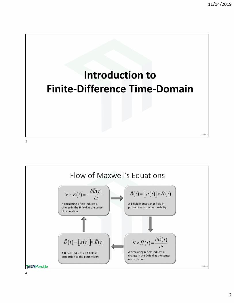
Flow of Maxwell’s Equations

Slide 4

B tE t

t

B t t H t

D tH t

t

D t t E t

A circulating E field induces a change in the B field at the center of circulation.

A B field induces an H field in proportion to the permeability.

A circulating H field induces a change in the D field at the center of circulation.

A D field induces an E field in proportion to the permittivity.

3

4

11/14/2019

3

Flow of Maxwell’s Equations Inside Linear, Isotropic and Non‐Dispersive Materials

Slide 5

H tE t

t

E tH t

t

A circulating E field induces a change in the H field at the center of circulation in proportion to the permeability.

A circulating H field induces a change in the E field at the center of circulation in proportion to the permittivity.

In materials that are linear, isotropic and non‐dispersive we have

t t

In this case, the flow of Maxwell’s equations reduces to

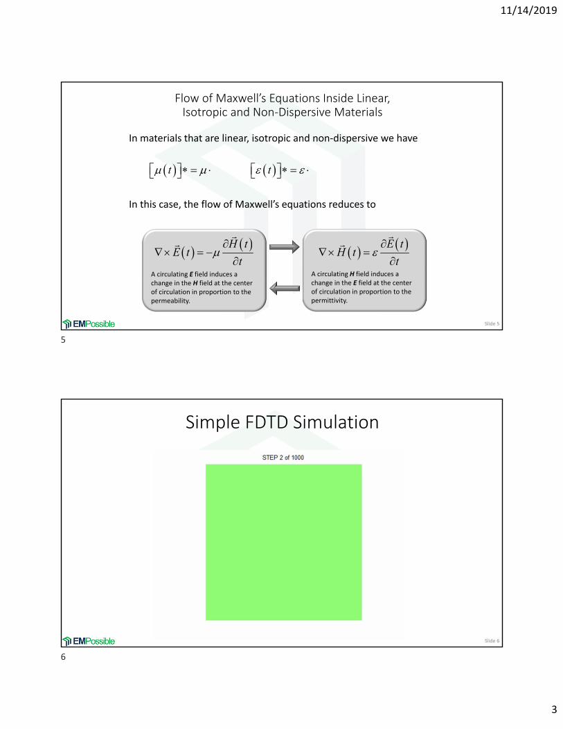
Simple FDTD Simulation

Slide 6

5

6

11/14/2019

4

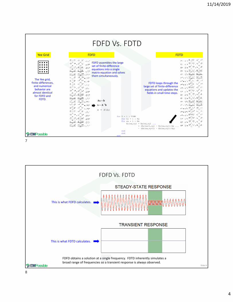
FDFD Vs. FDTDFDFD

FDFD assembles the large set of finite‐difference equations into a single matrix equation and solves them simultaneously.

1

Ax b

x A b

x = A\b;

for T = 1 : TIMEfor ny = 1 : Nyfor nx = 1 : Nx

Hz(nx,ny) = Hx(nx,ny) ...+ (Ey(nx+1,ny) - Ey(nx,ny))/dx ...- (Ex(nx,ny+1) - Ex(nx,ny))/dy;

endend

end

FDTD

FDTD loops through the large set of finite‐difference equations and updates the fields in small time steps.

Yee Grid

The Yee grid, finite‐differences, and numerical behavior are

almost identical for FDFD and

FDTD.

FDFD Vs. FDTD

Slide 8

This is what FDFD calculates.

This is what FDTD calculates.

FDFD obtains a solution at a single frequency. FDTD inherently simulates a broad range of frequencies so a transient response is always observed.

7

8

11/14/2019

5

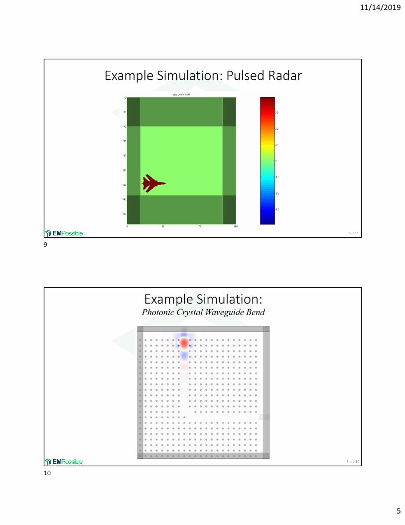
Example Simulation: Pulsed Radar

Slide 9

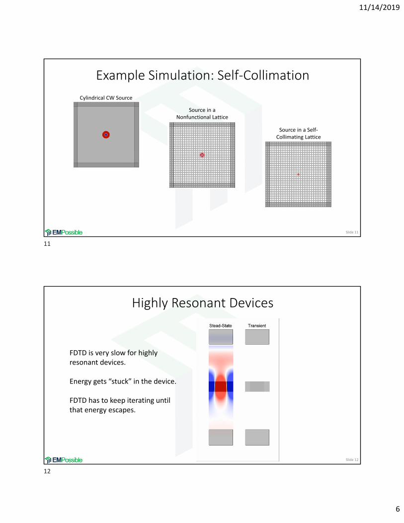
Example Simulation:Photonic Crystal Waveguide Bend

Slide 10

9

10

11/14/2019

6

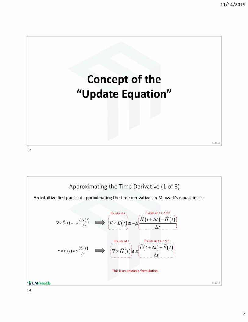
Example Simulation: Self‐Collimation

Slide 11

Cylindrical CW Source

Source in a Nonfunctional Lattice

Source in a Self‐Collimating Lattice

Highly Resonant Devices

Slide 12

FDTD is very slow for highly resonant devices.

Energy gets “stuck” in the device.

FDTD has to keep iterating until that energy escapes.

11

12

11/14/2019

7

Slide 13

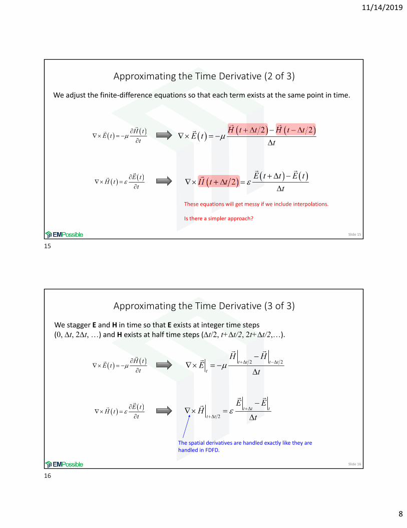
Concept of the“Update Equation”

Approximating the Time Derivative (1 of 3)

Slide 14

H tE t

t

E tH t

t

H t t H tE t

t

E t t E tH t

t

An intuitive first guess at approximating the time derivatives in Maxwell’s equations is:

This is an unstable formulation.

Exists at 2t t Exists at t

Exists at 2t t Exists at t

13

14

11/14/2019

8


Slide 15

H tE t

t

E tH t

t

2 2H t t H t tE t

t

2

E t t E tH t t

t

We adjust the finite‐difference equations so that each term exists at the same point in time.

These equations will get messy if we include interpolations.

Is there a simpler approach?


Slide 16

H tE t

t

E tH t

t

2 2t t t t

t

H HE

t

2

t t t

t t

E EH

t

We stagger E and H in time so that E exists at integer time steps (0, t, 2t, …) and H exists at half time steps (t/2, t+t/2, 2t+t/2,…).

The spatial derivatives are handled exactly like they are handled in FDFD.

15

16

11/14/2019

9

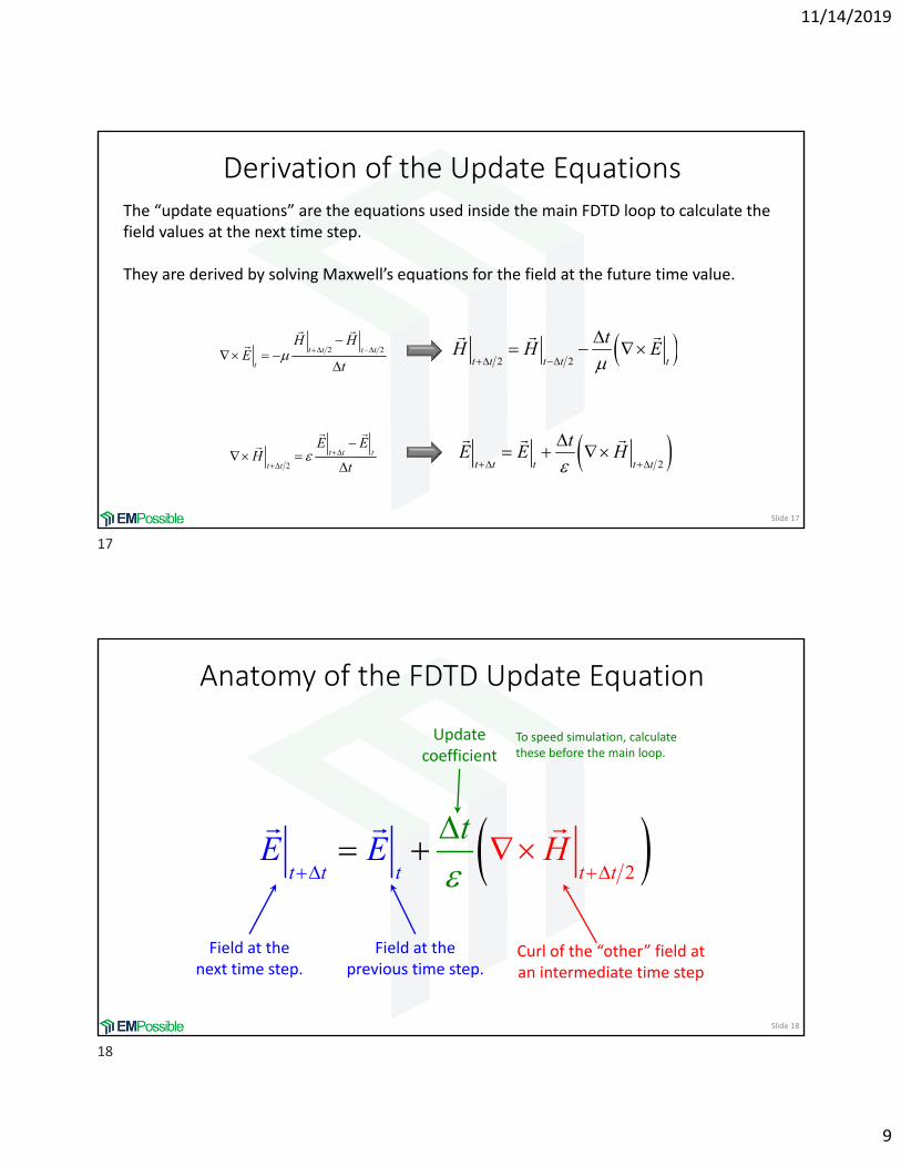
Derivation of the Update Equations

Slide 17

The “update equations” are the equations used inside the main FDTD loop to calculate the field values at the next time step.

They are derived by solving Maxwell’s equations for the field at the future time value.

2 2t t t t

t

H HE

t

2

t t t

t t

E EH

t

2 2t t t t t

tH H E

2t t t t t

tE E H

Anatomy of the FDTD Update Equation

Slide 18

2t tt t t

tHE E

Field at the next time step.

Field at the previous time step.

Curl of the “other” field at an intermediate time step

Update coefficient

To speed simulation, calculate these before the main loop.

17

18

11/14/2019

10

Slide 19

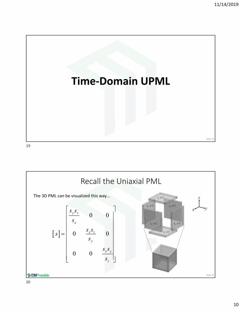
Time‐Domain UPML

Recall the Uniaxial PML

Slide 20

The 3D PML can be visualized this way…

0 0

0 0

0 0

y z

x

x z

y

x y

z

s s

s

s ss

s

s s

s

1zs

1zs

1xs

1xs 1ys

1ys x y

z

19

20

11/14/2019

11

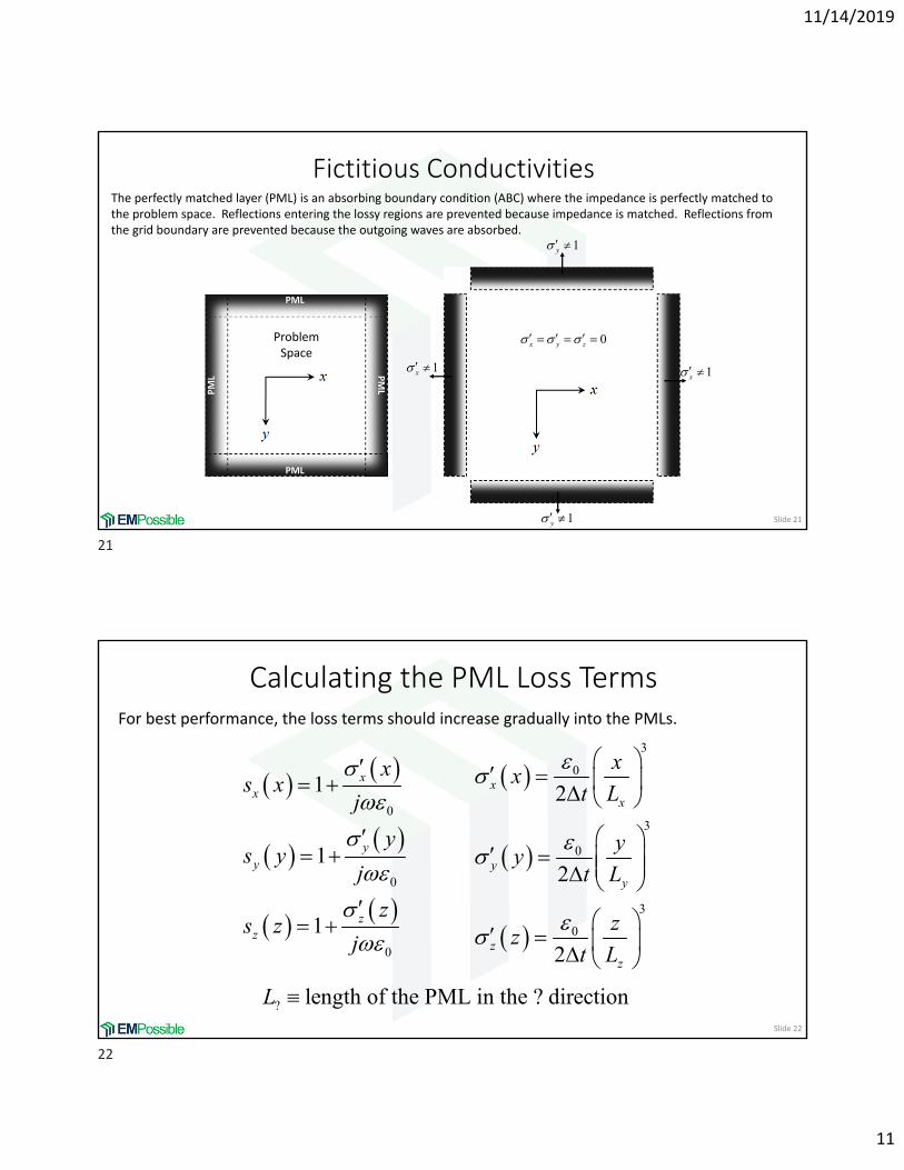
Fictitious Conductivities

Slide 21

PML

PML

PMLP

ML

ProblemSpace

1y

1x

0x y z

1y

1x

The perfectly matched layer (PML) is an absorbing boundary condition (ABC) where the impedance is perfectly matched to the problem space. Reflections entering the lossy regions are prevented because impedance is matched. Reflections from the grid boundary are prevented because the outgoing waves are absorbed.

Calculating the PML Loss Terms

Slide 22

For best performance, the loss terms should increase gradually into the PMLs.

3

0

3

0

3

0

2

2

2

xx

yy

zz

xx

t L

yy

t L

zz

t L

0

0

0

1

1

1

xx

yy

zz

xs x

j

ys y

j

zs z

j

? length of the PML in the ? directionL

21

22

11/14/2019

12

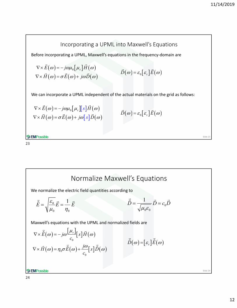
Incorporating a UPML into Maxwell’s Equations

Slide 23

0 rE j H

H E j D

0 rD E

Before incorporating a UPML, Maxwell’s equations in the frequency‐domain are

We can incorporate a UPML independent of the actual materials on the grid as follows:

0 rE j H

H E j D

s

s

0 rD E

Normalize Maxwell’s Equations

Slide 24

We normalize the electric field quantities according to

Maxwell’s equations with the UPML and normalized fields are

r

0

00

E j s Hc

jH E s D

c

rD E

0

0 0

1E E E

0

0 0

1D D c D

23

24

11/14/2019

13

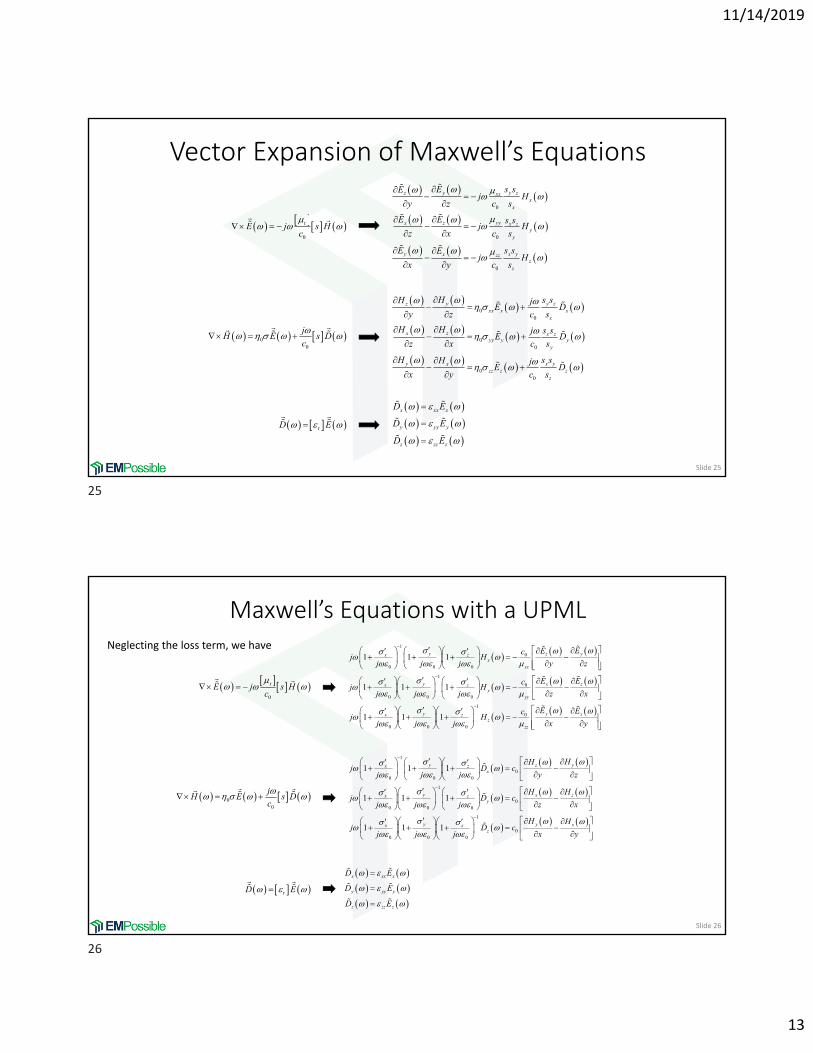
Vector Expansion of Maxwell’s Equations

Slide 25

0

0

0

y y zz xxx

x

yyx z x zy

y

y x yx zzz

z

E s sEj H

y z c s

E E s sj H

z x c s

E s sEj H

x y c s

x xx x

y yy y

z zz z

D E

D E

D E

00

00

00

y y zzxx x x

x

x z x zyy y y

y

y x yxzz z z

z

H s sH jE D

y z c s

H H s sjE D

z x c s

H s sH jE D

x y c s

r

0

E j s Hc

rD E

00

jH E s D

c

Maxwell’s Equations with a UPML

Slide 26

1

0

0 0 0

1

0

0 0 0

0 0

1 1 1

1 1 1

1 1 1

y yzx zx

xx

y x zx zy

yy

yx z

EEcj H

j j j y z

E Ecj H

j j j z x

jj j j

1

0

0

y xz

zz

E EcH

x y

x xx x

y yy y

z zz z

D E

D E

D E

1

00 0 0

1

00 0 0

1

0 0 0

1 1 1

1 1 1

1 1 1

y yzx zx

y x zx zy

yx z

HHj D c

j j j y z

H Hj D c

j j j z x

jj j j

0

y xz

H HD c

x y

r

0

E j s Hc

rD E

00

jH E s D

c

Neglecting the loss term, we have

25

26

11/14/2019

14

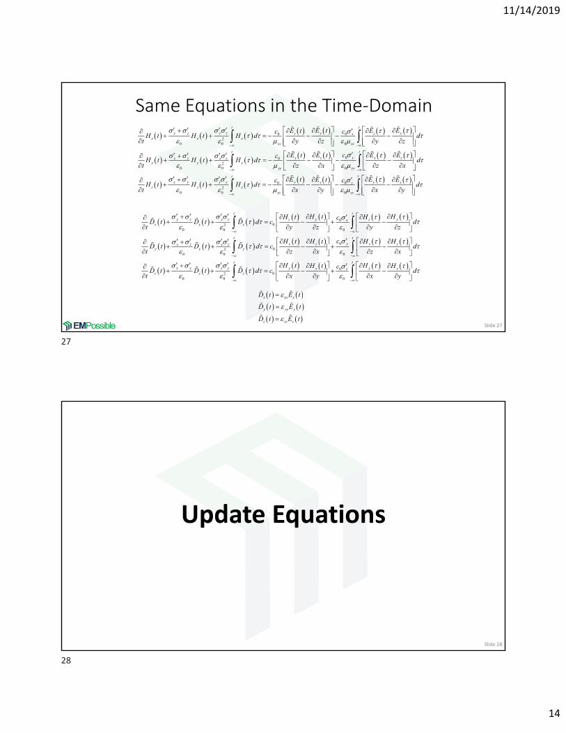
Same Equations in the Time‐Domain

Slide 27

0 02

0 0 0

002

0 0 0

t t

y z y z y yz zxx x x

xx xx

t

yx z x zx z x zy y y

yy yy

E t EE t Ec cH t H t H d d

t y z y z

cE t E t E EcH t H t H d

t z x z x

0 02

0 0 0

t

t t

x y x y y yx xzz z z

zz zz

d

E t EE t Ec cH t H t H d d

t x y x y

002

0 0 0

002

0 0 0

t t

y z y z y yz zxx x x

t t

yx z x zx z x zy y y

z

H t HH t HcD t D t D d c d

t y z y z

cH t H t H HD t D t D d c d

t z x z x

D tt

002

0 0 0

t t

x y x y y yx xzz z

H t HH t HcD t D d c d

x y x y

x xx x

y yy y

z zz z

D t E t

D t E t

D t E t

Slide 28

Update Equations

27

28

11/14/2019

15

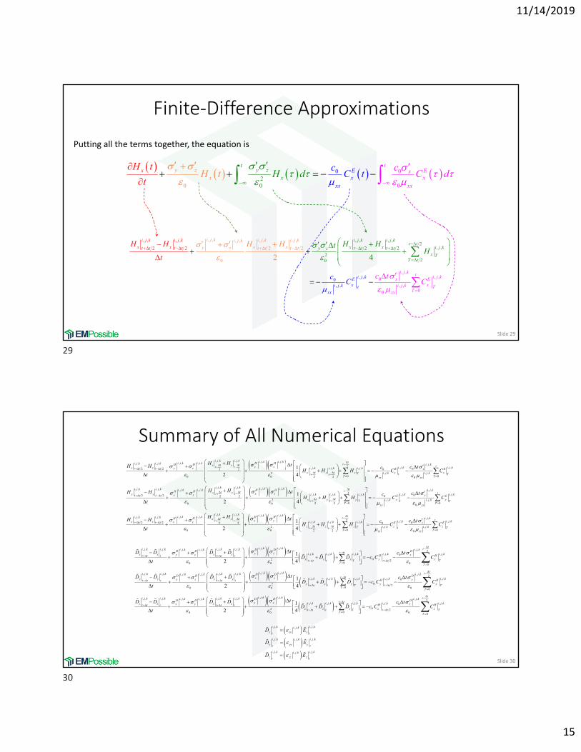
Finite‐Difference Approximations

Slide 29

Putting all the terms together, the equation is

0

0

0

002

tExx

x

ty E

xxx

xzzx y

xx

cCH d

cH t

H t

tC t d

, , , , , ,, ,

2

, , , ,

2 2

, , , ,2

, ,2 2

20

2

0 2

2 4

i j k i j kt t

x x i j kt t t

i j k i j k i j ki j kx xy z t t

i j k i j k

x x tt t t y zx T

t

t t t

T

H H

tH

H HtH H

, ,

, ,0, ,

, ,0,

00

, i j kE

xi j k tx

i j k t i j kx Exi j k T

xx Tx

cC

c tC

Summary of All Numerical Equations

Slide 30

, , , , , , , ,, , , ,, , , , , ,2 , ,, , , , , ,2 2 002 2

, ,200 0 2 2

1

2 4

i j k i j k i j k i j k ti j k i j k H Hi j k i j k t i j kH H t tx x y zt t i j kx x i j k i j k i j ky zt t t t xEt tx x x xi j kT tt t

T xx

H H tH H c tcH H H C

t

, ,

, ,00

, , , , , , , ,, , , , , , , ,2, , , , , ,2 2 02 2

,202 20 0

1

2 4

t i j kExi j k T

Txx

i j k i j k i j k i j k ti j k i j k i j k i j k H H tH H t ty y x zt ty y i j k i j k i j kx zt t t tt ty y y i jt t T

Tyy

C

H H tH H cH H H

t

, ,

, , , ,0

, , ,0

0

, , , , , , , ,, , , ,, , , ,

, , , , , ,2 2 2 22

00 0 2 2

1

2 4

i j kti j k i j kyE E

y yk i j kt TT

yy

i j k i j k i j k i j ki j k i j k H Hi j k i j k tH H t tz z x yt tz z i j k i j k i j kx yt t t tt tz z z Tt t

T

c tC C

H H tH HH H H

t

, ,2 , , , ,00

, , , ,00

ti j k ti j k i j kzE E

z zi j k i j kt TTzz zz

c tcC C

, , , ,, , , , , , , ,, , , , , , 2

, , , , , , , , , ,0

02 200 0 0 0

1

2 4

ti j k i j k ti j k i j k i j k i j ki j k i j k i j kD DD D Dt ty z i j k i j k i j k i j k i j kx x x xy z xH Ht t t t t tx x x x xt t Tt t t T

TT

y

tD D D D c tD D D c C C

t

D

, , , ,, , , , , , , ,, , , , , , 2

, , , , , , , , , ,0

02 200 0 0 0

1

2 4

ti j k i j k ti j k i j k i j k i j ki j k i j k i j kD DD D Dt tx z i j k i j k i j k i j k i j ky y yx z yH Ht t t t t ty y y y yt t Tt t t T

TT

z t

tD D D c tD D D c C C

t

D

, , , ,, , , , , , , ,, , , , , , 2

, , , , , , , , , ,0

02 200 0 0 0

1

2 4

ti j k i j k ti j k i j k i j k i j ki j k i j k i j kD DD D Dt tx y i j k i j k i j k i j k i j kz z zx y zH Ht t t t tz z z z zt t Tt t t T

TT

tD D D c tD D D c C C

t

, , , ,, ,

, , , ,, ,

, , , ,, ,

i j k i j ki j k

x xx xt t

i j k i j ki j k

y yy yt t

i j k i j ki j k

z zz zt t

D E

D E

D E

29

30

11/14/2019

16

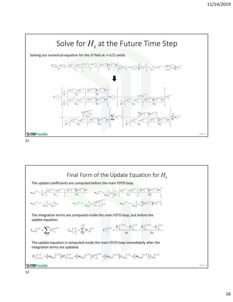
Solve for Hx at the Future Time Step

Slide 31

Solving our numerical equation for the H field at t+t/2 yields

, , , ,, , , ,

2 , ,0 0 , , 0

, , , ,, , , , , , , ,2

20

2

0

,

0

,

1

2 4

1 1

2 4 2

i j k i j ki j k i j k H HH Hy zy z

i j ki j k xx

txi j k i j k ti j k i j k i j k i j kH HH

i j k

H H Hy z yy z y

txt

z

t

t cH

t

t

H

t

, ,

, , , ,

20

, ,

, , , ,0, , 2

, ,0 0, , , ,, , , ,

0

20 0

4

+

1 1

2 4

i j kExi j k i j k tH H

z

i j kHx i j k i j kH H

ti j k y zi j kExx

xi j k i j k ti j k i j k H HH H HTy zy z y

Ct

c t t

Ct

t t

2

, ,

, , , ,, , , , 0

20 02 4

tt

i j k

xi j k i j k Ti j k i j k H HH Ty zz

Ht

, , , , , , , ,, , , ,, , , , , ,2 , ,, , , , , ,2 2 002 2

, ,200 0 2 2

1

2 4

i j k i j k i j k i j k ti j k i j k H Hi j k i j k t i j kH H t tx x y zt t i j kx x i j k i j k i j ky zt t t t xEt tx x x xi j kT tt t

T xx

H H tH H c tcH H H C

t

, ,

, ,00

t i j kExi j k T

Txx

C

Final Form of the Update Equation for Hx

Slide 32

, , , , , , , ,, , , , , , , ,

, , , ,

0 1 , ,2 20 0 0 00

, , 02 , , , ,

0

1 1 1

2 4 2 4

1

i j k i j k i j k i j ki j k i j k i j k i j kH H H HH H H Hy z y zi j k i j ky z y z

Hx Hx i j k

Hx

i j k

Hx i j k i j k

Hx xx

t tm m

t tm

cm

m

, ,

, , , ,, , , ,03 4, , , , , , 2

0 00 0

1 1

i j kHi j k i j ki j k i j kx H H

Hx Hx y zi j k i j k i j k

Hx xx Hx

c t tm m

m m

, ,, , , , , , , , , , , , , ,

1 2 3 42

, ,

2

i j ki j k i j k i j k i j k i j k i j k i j kEHx x Hx x H

i j k

x x CEx Hx Hxt t t ttt tm H m C m I m IH

, 1, , , , , 1 , ,2, , , ,, , , , , ,

020

t i j k i j k i j k i j ktti j k i j k z z y yi j k i j k i j kE E t t t t

CEx x Hx t x xt Tt tt TT

E E E EI C I H C

y z

The update coefficients are computed before the main FDTD loop.

The integration terms are computed inside the main FDTD loop, but before the update equation.

The update equation is computed inside the main FDTD loop immediately after the integration terms are updated.

31

32

11/14/2019

17

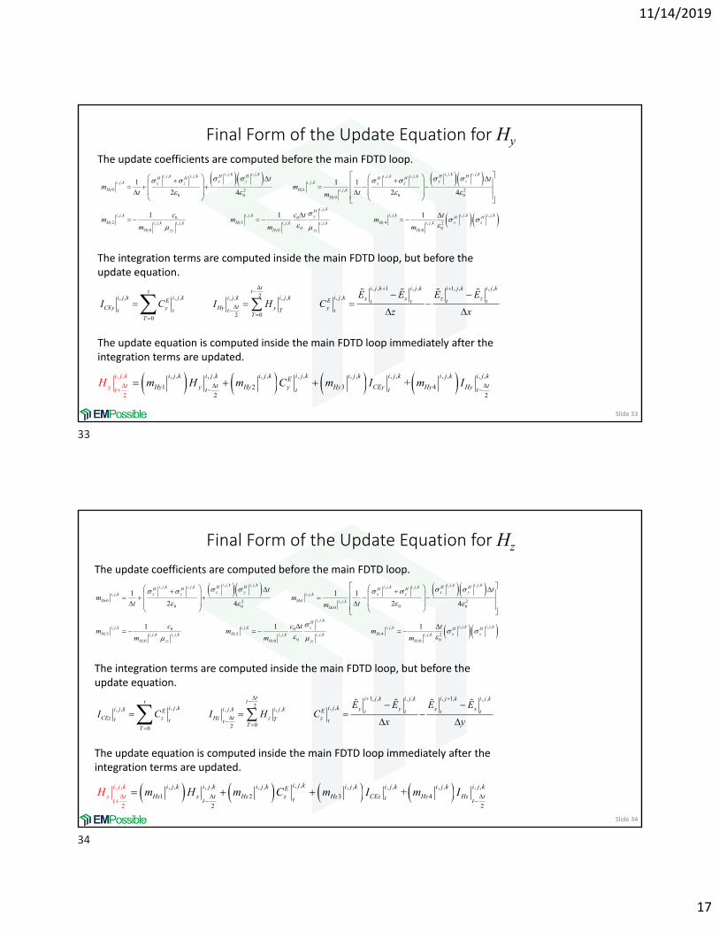
Final Form of the Update Equation for Hy

Slide 33

, , , , , , , ,, , , , , , , ,

, , , ,

0 1 , ,2 20 0 0 00

, ,0

2 , , , ,

0

1 1 1

2 4 2 4

1

i j k i j k i j k i j ki j k i j k i j k i j kH H H HH H H Hx z x zi j k i j kx z x z

Hy Hy i j k

Hy

i j k

Hy i j k i j k

Hy yy

t tm m

t tm

cm

m

, ,

, , , ,, , , ,0

3 4, , , , , , 20 00 0

1 1

i j kHi j k i j ki j k i j ky H H

Hy Hy x zi j k i j k i j k

Hy yy Hy

c t tm m

m m

, ,, , , , , , , , , , , , , ,

1 2 3 4

,

2 2

,

2

+i j ki j k i j k i j k i j k i j k i j k i j kE

t tHy y Hy y Hy CEy Hy Hy

i j

t

k

t tt

ty tm H m C m I m IH

, , 1 , , 1, , , ,2, , , ,, , , , , ,

020

t i j k i j k i j k i j ktti j k i j ki j k i j k i j k x x z zE E t t t t

tCEy y Hy y yt t Tt tT

T

E E E EI C I H C

z x




Final Form of the Update Equation for Hz

Slide 34

, , , , , , , ,, , , , , , , ,

, , , ,

0 12 , , 20 00 00

, , 02 , , , ,

0

1 1 1

2 24 4

1

i j k i j k i j k i j ki j k i j k i j k i j kH H H HH H H Hx y x yx y x yi j k i j k

Hz Hz i j k

Hz

i j k

Hz i j k i j k

Hz zz

t tm m

t tm

cm

m

, ,

, , , ,, , , ,03 4, , , , , , 2

0 00 0

1 1

i j kHi j k i j kzi j k i j k H H

Hz Hz x yi j k i j k i j k

Hz zz Hz

c t tm m

m m

, ,, , , , , , , , , , , , , ,

1 2 3 4

,

2 2

,

2

+i j ki j k i j k i j k i j k i j k i j k i j kE

Hz z t Hz z Hz CEz Hz Hz

i j k

z tt

tttt tm H m C m I m IH

1, , , , , 1, , ,2, , , ,, , , , , ,

020

t i j k i j k i j k i j ktti j k i j k y y x xi j k i j k i j kE E t t t t

tCEz z Hz z zt Tt ttT

T

E E E EI C I H C

x y




33

34

11/14/2019

18

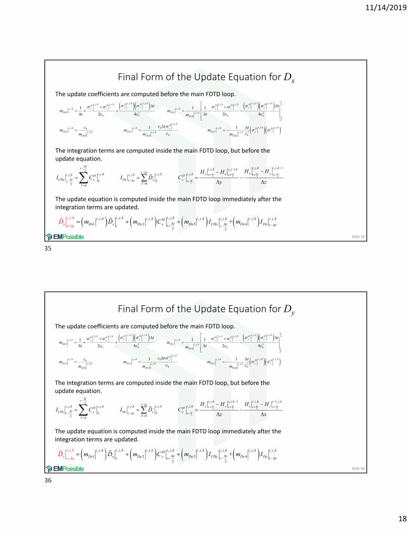
Final Form of the Update Equation for Dx

Slide 35

, , , , , , , ,, , , , , , , ,

, , , ,

0 1 , ,2 20 0 0 00

, , , ,02 3, ,

0

1 1 1

2 4 2 4

i j k i j k i j k i j ki j k i j k i j k i j kD D D DD D D Dy z y zi j k i j ky z y z

Dx Dx i j k

Dx

i j k i j

Dx Dxi j k

Dx

t tm m

t tm

cm m

m

, ,

, , , ,, ,0

4, , , , 20 00 0

1 1

i j kDi j k i j kk i j kx D D

Dx y zi j k i j k

Dx Dx

c t tm

m m

, , , ,, , , , , , , , , , , ,

1 2 3 42

, ,

2

+i j k i j ki j k i j k i j k i j k i j k i j kH

t tDx x Dx x Dx CHx D

i j

x Dx t tt

k

x t t t tm D m C m I m ID

2 2 2 2

2

, , , , 1, , , 1,2, ,, , , ,, , , ,

02 0

t t t t

t

t i j k i j kt i j k i j kt t y yi j ki j k i j k z zi j k i j k t t t tH H

tCHx x Dx x xt tT tTtT

T

H HH HI C I D C

y z




Final Form of the Update Equation for Dy

Slide 36

, , , , , , , ,, , , , , , , ,

, , , ,

0 1 , ,2 20 0 0 00

, , , ,0

2 3, ,

0

1 1 1

2 4 2 4

i j k i j k i j k i j ki j k i j k i j k i j kD D D DD D D Dx z x zi j k i j kx z x z

Dy Dy i j k

Dy

i j k i j

Dy Dyi j k

Dy

t tm m

t tm

cm m

m

, ,

, , , ,, ,0

4, , , , 20 00 0

1 1

i j kDi j k i j kk i j ky D D

Dy x zi j k i j k

Dy Dy

c t tm

m m

, , , ,, , , , , , , , , , , ,

1 2 3 422

, ,+

i j k i j ki j k i j k i j k i j k i j k i j kHttDy y Dy y Dy CHy D

i j

y Dyt t tt

k

y t t tm D m C m I m ID

2 2 2 2

2

, , , , 1 , , 1, ,2, ,, , , ,, , , ,

020

t t t t

t

tt i j k i j k i j k i j k

t t i j ki j k i j k x x z zi j k i j k t t t tH HtCHy y Dy y yt t tT tT

TT

H H H HI C I D C

z x




35

36

11/14/2019

19

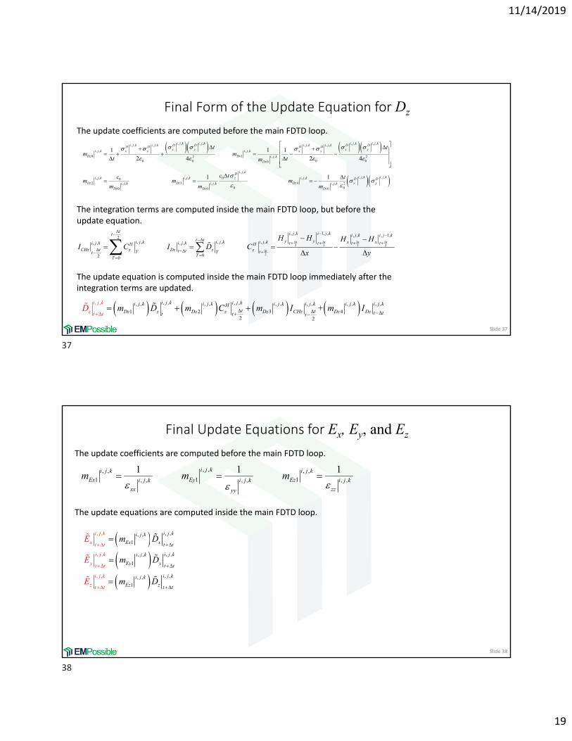
Final Form of the Update Equation for Dz

Slide 37

, , , , , , , ,, , , , , , , ,

, , , ,

0 1 , ,2 20 0 0 00

, , , ,02 3, ,

0

1 1 1

2 4 2 4

i j k i j k i j k i j ki j k i j k i j k i j kD D D DD D D Dx y x yi j k i j kx y x y

Dz Dx i j k

Dx

i j k i j

Dz Dzi j k

Dz

t tm m

t tm

cm m

m

, ,

, , , ,, ,0

4, , , , 20 00 0

1 1

i j kDi j k i j kk i j kz D D

Dz x yi j k i j k

Dz Dz

c t tm

m m

, , , ,, , , , , , , , , , , ,

1 2 3 42

, ,

2

+i j k i j ki j k i j k i j k i j k i j k i j kH

t tDz z Dz z Dz CHz D

i j

z Dz t tt

k

z t t t tm D m C m I m ID

2 2 2 2

2

, , 1, , , , , 1,2, ,, , , ,, , , ,

02 0

t t t t

t

t i j k i j kt i j k i j kt t y yi j ki j k i j k x xi j k i j k t t t tH H

tCHz z Dz z zt tT tTtT

T

H H H HI C I D C

x y




Final Update Equations for Ex, Ey, and Ez

Slide 38

, ,, , , ,

1 1 1, , , , , ,

1 1 1

i j ki j k i j k

Ex Ey Ezi j k i j k i j k

xx zzyy

m m m

, ,, ,

1

, ,, ,

1

, ,, ,

1

, ,

, ,

, ,

i j ki j k

Ex x t t

i j ki j k

i j k

x t

Ey y t t

i j ki j k

E

t

i j k

y t t

i j k

z z t tz t t

E

E

E

m D

m D

m D


The update equations are computed inside the main FDTD loop.

37

38

11/14/2019

20

Slide 39

Total‐Field/Scattered‐Field Source

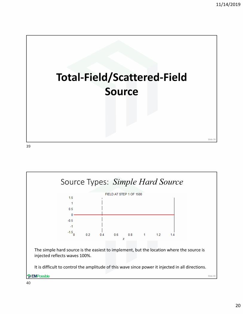
Source Types: Simple Hard Source

Slide 40

The simple hard source is the easiest to implement, but the location where the source is injected reflects waves 100%.

It is difficult to control the amplitude of this wave since power it injected in all directions.

39

40

11/14/2019

21

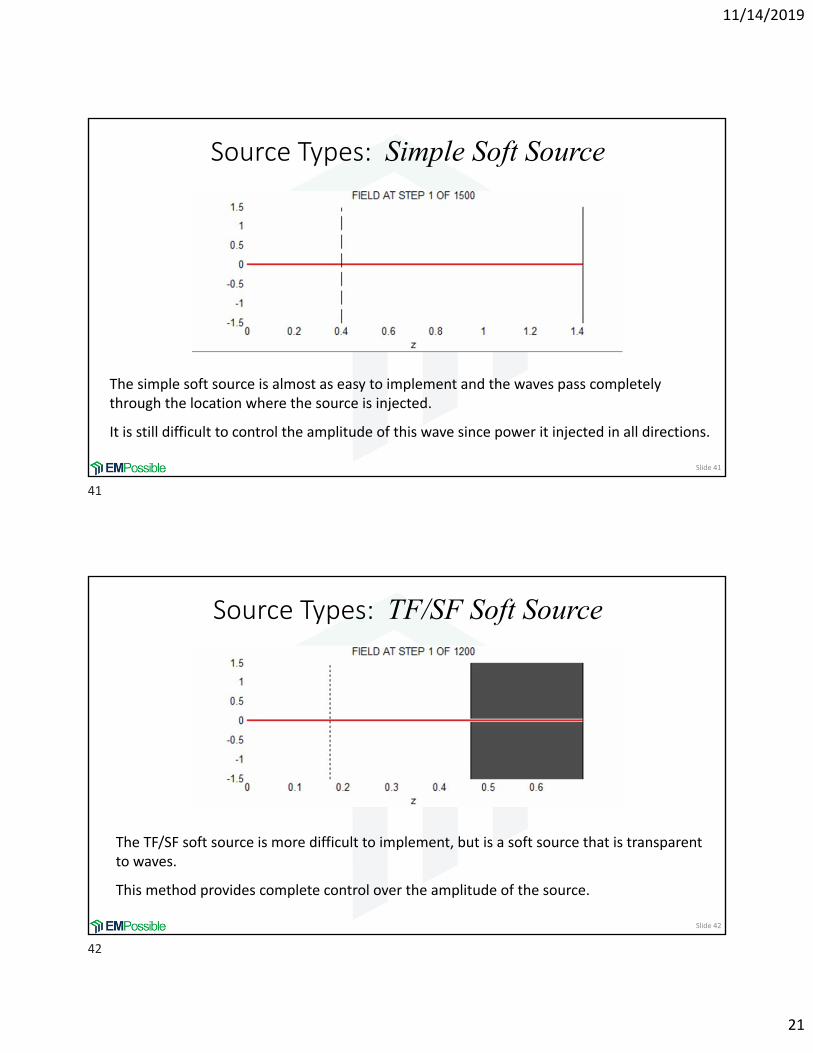
Source Types: Simple Soft Source

Slide 41

The simple soft source is almost as easy to implement and the waves pass completely through the location where the source is injected.

It is still difficult to control the amplitude of this wave since power it injected in all directions.

Source Types: TF/SF Soft Source

Slide 42

The TF/SF soft source is more difficult to implement, but is a soft source that is transparent to waves.

This method provides complete control over the amplitude of the source.

41

42

11/14/2019

22

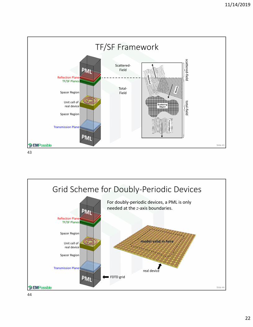
TF/SF Framework

Slide 43

scattered‐field

total‐field

Reflection PlaneTF/SF Planes

Unit cell of real device

Spacer Region

Spacer Region

Transmission Plane

Scattered‐Field

Total‐Field

Grid Scheme for Doubly‐Periodic Devices

Slide 44

For doubly‐periodic devices, a PML is only needed at the z‐axis boundaries.

FDTD grid

real device



Spacer Region

Spacer Region

Transmission Plane

model valid in here

43

44

11/14/2019

23

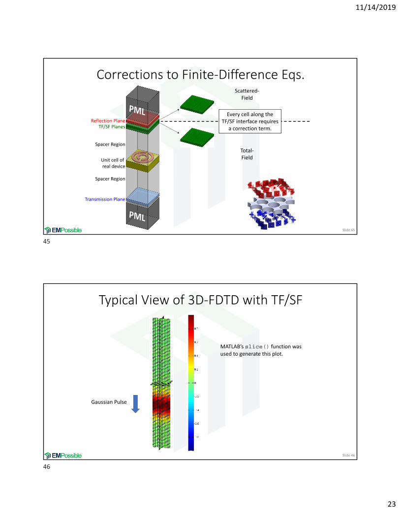
Corrections to Finite‐Difference Eqs.

Slide 45



Spacer Region

Spacer Region

Transmission Plane

Scattered‐Field

Total‐Field

Every cell along the TF/SF interface requires

a correction term.

Typical View of 3D‐FDTD with TF/SF

Slide 46

Gaussian Pulse

MATLAB’s slice() function was used to generate this plot.

45

46

11/14/2019

24

Slide 47

Calculating Steady‐State Fields

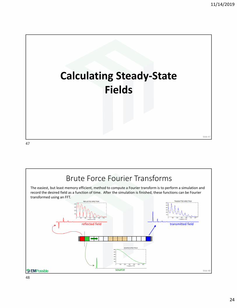
Brute Force Fourier Transforms

Slide 48

The easiest, but least memory efficient, method to compute a Fourier transform is to perform a simulation and record the desired field as a function of time. After the simulation is finished, these functions can be Fourier transformed using an FFT.

source

reflected field transmitted field

47

48

11/14/2019

25

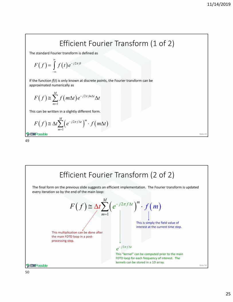
Efficient Fourier Transform (1 of 2)

Slide 49

The standard Fourier transform is defined as

2j ftF f f t e

If the function f(t) is only known at discrete points, the Fourier transform can be approximated numerically as

2

1

Mj fm t

m

F f f m t e t

This can be written in a slightly different form.

2

1

M mj f t

m

F f t e f m t

Efficient Fourier Transform (2 of 2)

Slide 50

The final form on the previous slide suggests an efficient implementation. The Fourier transform is updated every iteration so by the end of the main loop:

2

1

fM

t m

m

j f meF f t

2j f te

This “kernel” can be computed prior to the main FDTD loop for each frequency of interest. The kernels can be stored in a 1D array.

This is simply the field value of interest at the current time step.

This multiplication can be done after the main FDTD loop in a post‐processing step.

49

50

11/14/2019

26

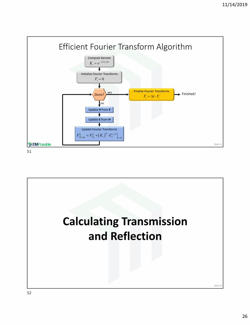
Efficient Fourier Transform Algorithm

Slide 51

Finished!

Compute Kernels2 ij f t

iK e

Update H from E

no

Update Fourier Transforms

Done?yes

Update E from H

Initialize Fourier Transforms

0iF

, ,m i j ki i i yt t t t t

F F K E

Finalize Fourier Transforms

i iF t F

Slide 52

Calculating Transmission and Reflection

51

52

11/14/2019

27

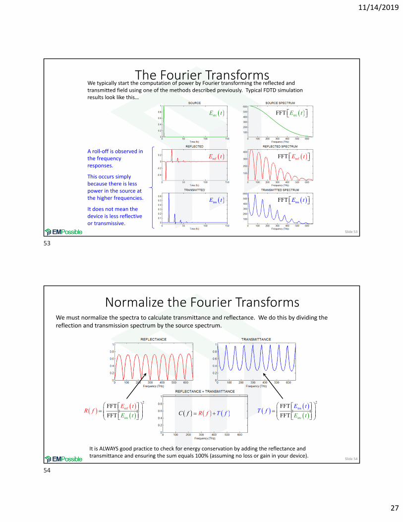
The Fourier Transforms

Slide 53

We typically start the computation of power by Fourier transforming the reflected and transmitted field using one of the methods described previously. Typical FDTD simulation results look like this…

srcFFT E t

trnFFT E t

refFFT E t

srcE t

trnE t

refE tA roll‐off is observed in the frequency responses.

This occurs simply because there is less power in the source at the higher frequencies.

It does not mean the device is less reflective or transmissive.

Normalize the Fourier Transforms

Slide 54

We must normalize the spectra to calculate transmittance and reflectance. We do this by dividing the reflection and transmission spectrum by the source spectrum.

It is ALWAYS good practice to check for energy conservation by adding the reflectance and transmittance and ensuring the sum equals 100% (assuming no loss or gain in your device).

sr

re

c

2

fFFT

FFT E t

E tR f

sr

tr

c

2

nFFT

FFT E t

E tT f

C f TR f f

53

54

11/14/2019

28

Slide 55

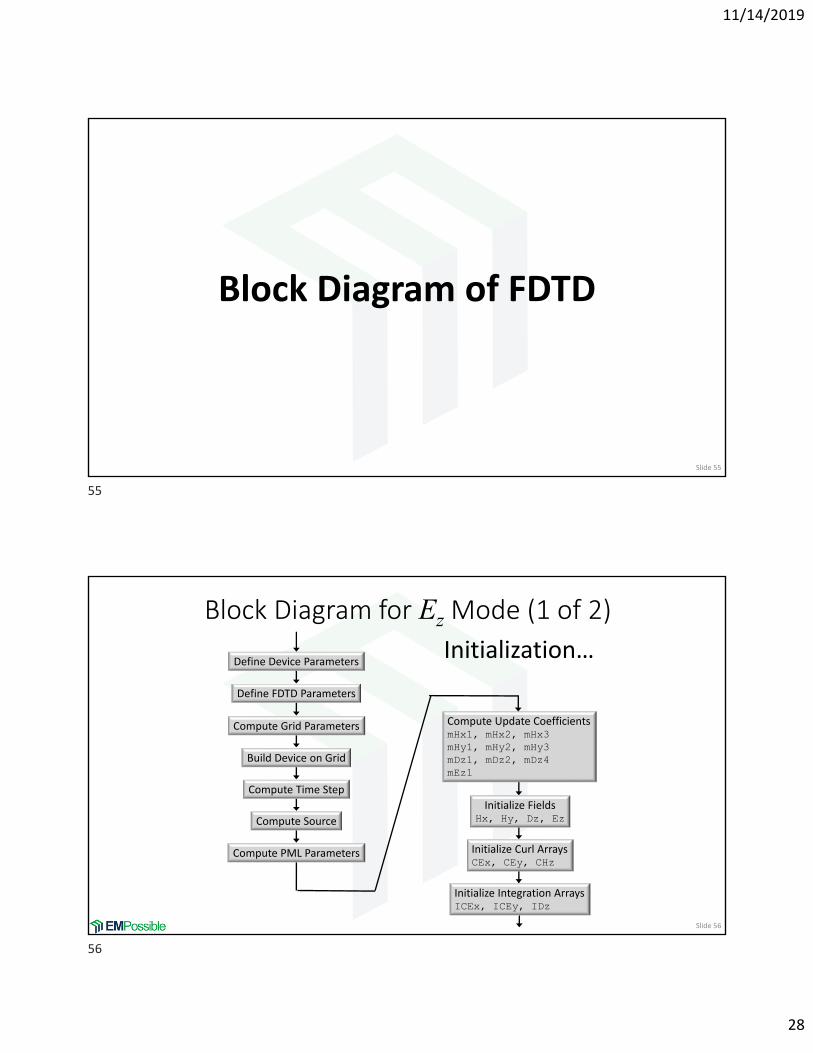
Block Diagram of FDTD

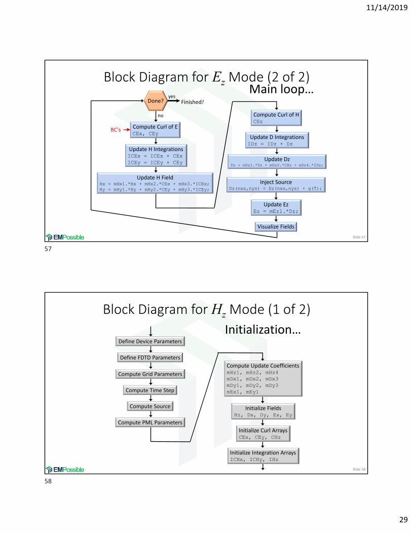
Block Diagram for Ez Mode (1 of 2)

Slide 56

Define Device Parameters

Define FDTD Parameters

Compute Grid Parameters

Compute Time Step

Compute Source

Compute PML Parameters

Compute Update CoefficientsmHx1, mHx2, mHx3mHy1, mHy2, mHy3mDz1, mDz2, mDz4mEz1

Initialize FieldsHx, Hy, Dz, Ez

Initialize Curl ArraysCEx, CEy, CHz

Initialize Integration ArraysICEx, ICEy, IDz

Initialization…

Build Device on Grid

55

56

11/14/2019

29

Block Diagram for Ez Mode (2 of 2)

Slide 57

Compute Curl of ECEx, CEy

Update H IntegrationsICEx = ICEx + CExICEy = ICEy + CEy

Update H FieldHx = mHx1.*Hx + mHx2.*CEx + mHx3.*ICEx;Hy = mHy1.*Hy + mHy2.*CEy + mHy3.*ICEy;

Update EzEz = mEz1.*Dz;

Visualize Fields

Main loop…

Compute Curl of HCHz

Update D IntegrationsIDz = IDz + Dz

Inject SourceDz(nxs,nys) = Dz(nxs,nys) + g(T);

Finished!yes

Done?

no

Update DzDz = mDz1.*Dz + mDz2.*CHz + mDz4.*IDz;

BC’s

Block Diagram for Hz Mode (1 of 2)

Slide 58

Define Device Parameters

Define FDTD Parameters

Compute Grid Parameters

Compute Time Step

Compute Source

Compute PML Parameters

Compute Update CoefficientsmHz1, mHz2, mHz4mDx1, mDx2, mDx3mDy1, mDy2, mDy3mEx1, mEy1

Initialize FieldsHz, Dx, Dy, Ex, Ey

Initialize Curl ArraysCEx, CEy, CHz

Initialize Integration ArraysICHx, ICHy, IHz

Initialization…

57

58

11/14/2019

30

Update E FieldEx = mEx1.*Dx;Ey = mEy1.*Dy;

Block Diagram for Hz Mode (2 of 2)

Slide 59

Compute Curl of ECEz

Update H IntegrationsIHz = IHz + Hz

Update H FieldHz = mHz1.*Hz + mHz2.*CEz + mHz4.*IHz;

Update D FieldDx = mDx1.*Dx + mDx2.*CHx + mDx3.*ICHx;Dy = mDy1.*Dy + mDy2.*CHy + mDy3.*ICHy;

Main loop…

Compute Curl of HCHx, CHy

Update D IntegrationsICHx = ICHx + CHx;ICHy = ICHy + CHy;

Inject SourceHz(nxs,nys) = Hz(nxs,nys) + g(T);

Finished!yes

Done?

no

Visualize Fields

BC’s

Slide 60

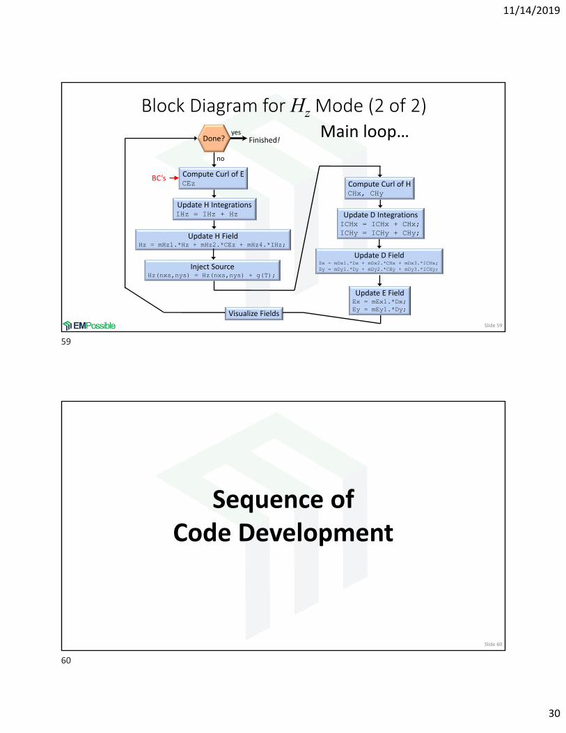
Sequence ofCode Development

59

60

11/14/2019

31

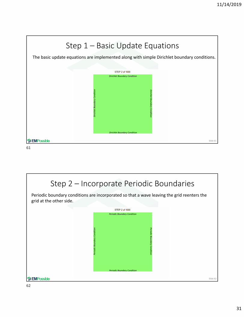
Step 1 – Basic Update Equations

Slide 61

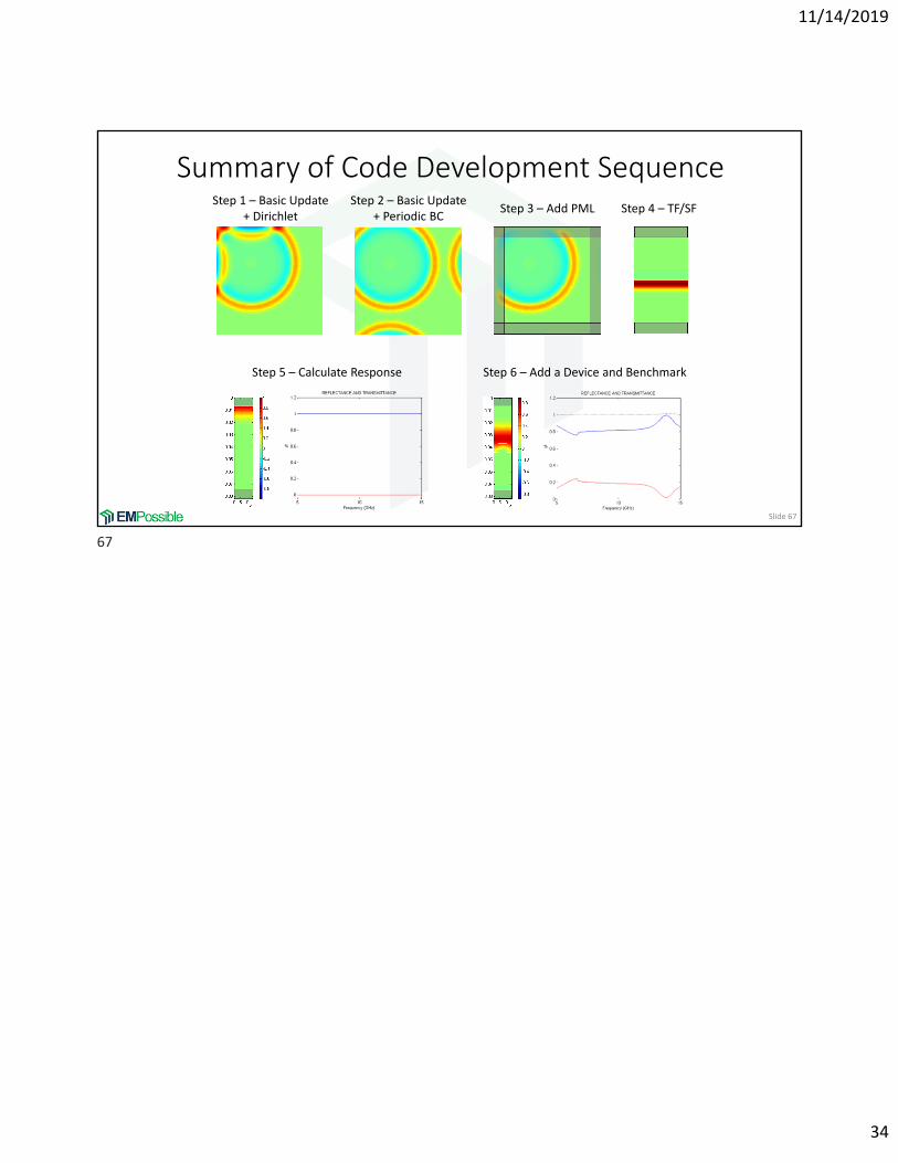
The basic update equations are implemented along with simple Dirichlet boundary conditions.

Dirichlet Boundary Condition

Dirichlet Boundary Condition

DirichletBoundary Condition D

irichlet

Boundary C

onditio

n

Step 2 – Incorporate Periodic Boundaries

Slide 62

Periodic boundary conditions are incorporated so that a wave leaving the grid reenters the grid at the other side.

Periodic Boundary Condition



Perio

dic B

oundary C

onditio

n

61

62

11/14/2019

32

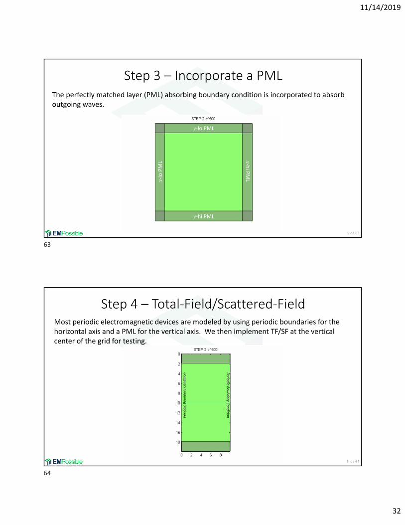
Step 3 – Incorporate a PML

Slide 63

The perfectly matched layer (PML) absorbing boundary condition is incorporated to absorb outgoing waves.

y‐lo PML

y‐hi PML

x‐hi PMLx‐

lo PML

Step 4 – Total‐Field/Scattered‐Field

Slide 64

Most periodic electromagnetic devices are modeled by using periodic boundaries for the horizontal axis and a PML for the vertical axis. We then implement TF/SF at the vertical center of the grid for testing.


Perio

dic B

oundary C

onditio

n

63

64

11/14/2019

33

Step 5 – Calculate TRN, REF, and CON

Slide 65

We move the TF/SF interface to a unit cell or two outside of the top PML. We include code to calculate Fourier transforms and to calculate transmittance, reflectance, and conservation of power.

Step 6 – Model a Device to Benchmark

Slide 66

We build a device on the grid that has a known solution. We run the simulation and duplicate the known results to benchmark our new code.

65

66

11/14/2019

34

Summary of Code Development Sequence

Slide 67

Step 1 – Basic Update + Dirichlet

Step 2 – Basic Update + Periodic BC

Step 3 – Add PML Step 4 – TF/SF

Step 5 – Calculate Response Step 6 – Add a Device and Benchmark

67

finite difference time (fdtd)

Documents