Nikolova 2009 1

THE FINITE-DIFFERENCE TIME-DOMAIN (FDTD) METHOD – PART IV

The Perfectly Matched Layer (PML) Absorbing Boundary Condition

Numerical Techniques in Electromagnetics ECE 757

Nikolova 2009 2

1. The need for good absorbers

good performance of the absorbers is crucial for(1) the accuracy of frequency-domain responses

(3) the analysis of low-RCS targets, low-reflection coatings, matched loads, etc.

(2) reducing the size of the computational domain

Mur and Liao absorbers provide effective reflection coefficientsof about 0.5 % to 5 %: errors above -40 dB are common

numerical errors below -40 dB (1/100) always desirable, sometimes -80 dB

Berenger publishes his first work on PML in 1994 reporting reflections of about 3000 times less than Mur’s 2nd order ABC!

Nikolova 2009 3

2. Theory of plane wave diffraction: review

We know that for reflection-free propagation through the interface between two mediums, their intrinsic impedances must be matched. The intrinsic impedance of a fictitious lossy medium which has both electric and magnetic conductivity is

ljj

μ μ μηε ε ε

′ ′′−= =

′ ′′−If , e mσ σε μ

ω ω′′ ′′= =

Let the lossy region be region 2 onto which plane waves are incident from region 1. Region 1 is loss-free and with real consti-tutive parameters ε, μ. Its intrinsic impedance is then . Let . The propagation constants are

/η μ ε=, ε ε μ μ′ ′= =

jγ ω εμ= and 1 1e ml j j jσ σγ ω εμ

ωε ωμ⎛ ⎞⎛ ⎞= − −⎜ ⎟⎜ ⎟⎝ ⎠⎝ ⎠

1

1

m

le

j

j

σμ ωμη σε

ωε

⎛ ⎞−′ ′⎜ ⎟⇒ = ⎜ ⎟′ −⎜ ⎟′⎝ ⎠

Nikolova 2009 4

2. Theory of plane wave diffraction, cont.

e mσ σε μ= !

is observed in the lossy medium, then , and a plane wave normally incident upon the interface is not reflected back! Moreover, the velocity of propagation is the same as in region 1:

lη η=

impedance matching condition

If the condition

l ejαβ

γ ω με ησ= +

and the medium is dispersion-free despite its losses.

Nikolova 2009 5

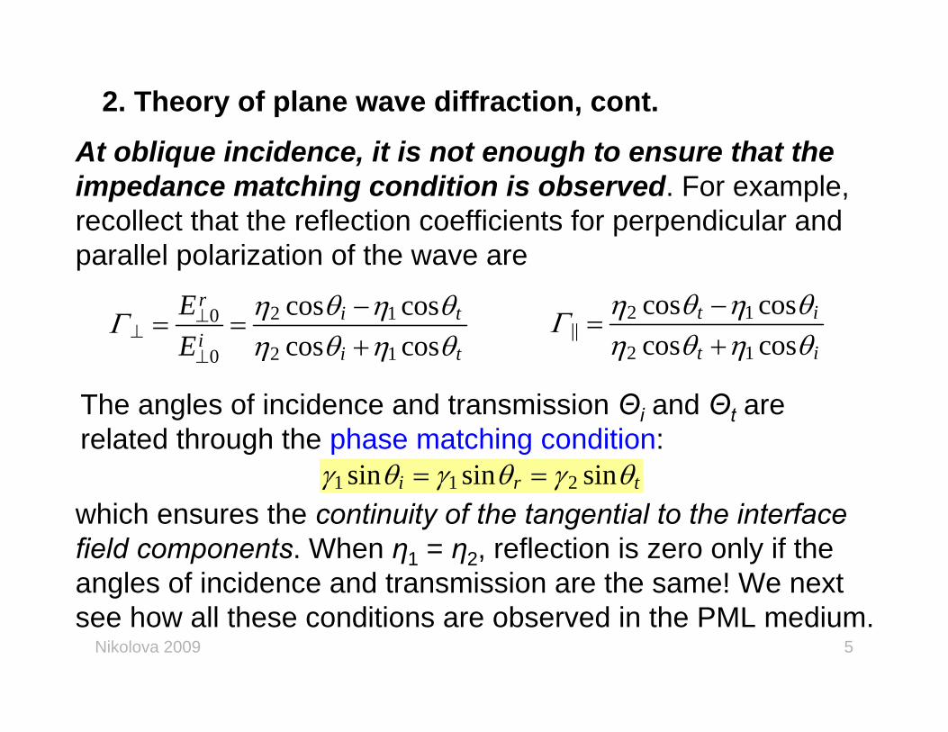
2. Theory of plane wave diffraction, cont.

At oblique incidence, it is not enough to ensure that the impedance matching condition is observed. For example, recollect that the reflection coefficients for perpendicular andparallel polarization of the wave are

2 10

2 10

cos coscos cos

ri t

ii t

EE

η θ η θΓη θ η θ

⊥⊥

⊥

−= =

+

The angles of incidence and transmission Θi and Θt are related through the phase matching condition:

1 1 2sin sin sini r tγ θ γ θ γ θ= =

2 1||

2 1

cos coscos cos

t i

t i

η θ η θΓη θ η θ

−=

+

which ensures the continuity of the tangential to the interface field components. When η1 = η2, reflection is zero only if the angles of incidence and transmission are the same! We next see how all these conditions are observed in the PML medium.

Nikolova 2009 6

3. Berenger’s Perfectly Matched Medium: TE Case

Maxwell’s equations for the TEz case (source-free): y xz

m zE EH H

t x yμ σ

∂⎛ ⎞∂∂ + = − −⎜ ⎟∂ ∂ ∂⎝ ⎠x z

e xE HEt y

ε σ∂ ∂+ =

∂ ∂

y ze y

E HEt x

ε σ∂ ∂

+ = −∂ ∂

Berenger splits the Hz field component:so that (look at the 1st equation), the x-derivative of Egenerates Hzx, and the y-derivative of E generates Hzy.

z zx zyH H H= +

He also introduces different specific conductivities to accompany the split terms.

Nikolova 2009 7

3. Berenger’s Perfectly Matched Medium: TE Case, cont.

xx

yzm zx

EH Hxt

μ σ∂∂

+ = −∂∂

( )zx zyxe xy

H HE Et y

ε σ∂ +∂

+ =∂∂

( )y zx zye yx

E H HE

t xε σ∂ ∂ +

+ = −∂∂

yy

z xm zy

H EHyt

μ σ∂ ∂

=∂ ∂

+

We next study the plane wave propagation in Berenger’s medium.

Nikolova 2009 8

4. Plane Waves in Berenger’s Medium: TE Case Let a time-harmonic plane TEz wave propagate as shown in the figure at an angle Φ with respect to the x-axis. The E-field then forms an angle Φ with respect to the y-axis.

1 1( )0 sin x yj t v x v y

xE E e ωφ− −− −= − ⋅

E

x

y

zˆ zH=H z

φ P

φ

1 1( )0 cos x yj t v x v y

yE E e ωφ− −− −= ⋅

1 1

0( )x yj t v x v y

zx zxH H e ω − −− −=1 1

0( )x yj t v x v y

zy zyH H e ω − −− −=

The constants vx and vy are complex. They describe the wave behavior in space and can be viewed as complex velocities. We find them by substituting the above field components in Berenger’s TEz equations.

Nikolova 2009 9

4. Plane Waves in Berenger’s Medium: TE Case, cont.

10 0 0sin ( )ey

y zx zyj E v H Hσ

ε φω

−⎛ ⎞− = +⎜ ⎟⎝ ⎠

10 0 0cos ( )ex

x zx zyj E v H Hσε φω

−⎛ ⎞− = +⎜ ⎟⎝ ⎠

xyzx

m zxEH Hxt

μ σ∂∂

+ = −∂∂

( )zx zyxe xy

H HE Et y

ε σ∂ +∂

+ =∂∂

( )y zx zye yx

E H HE

t xε σ∂ ∂ +

+ = −∂∂

100 cosmx

zx xj H v Eσμ φω

−⎛ ⎞− =⎜ ⎟⎝ ⎠

yzy x

m zyH EH

t yμ σ∂ ∂

+ =∂∂

100 sinmy

zy yj H v Eσ

μ φω

−⎛ ⎞− =⎜ ⎟⎝ ⎠

We express and from the last two equations and substitute them in the 1st two.

0zxH 0zyH

Nikolova 2009 10

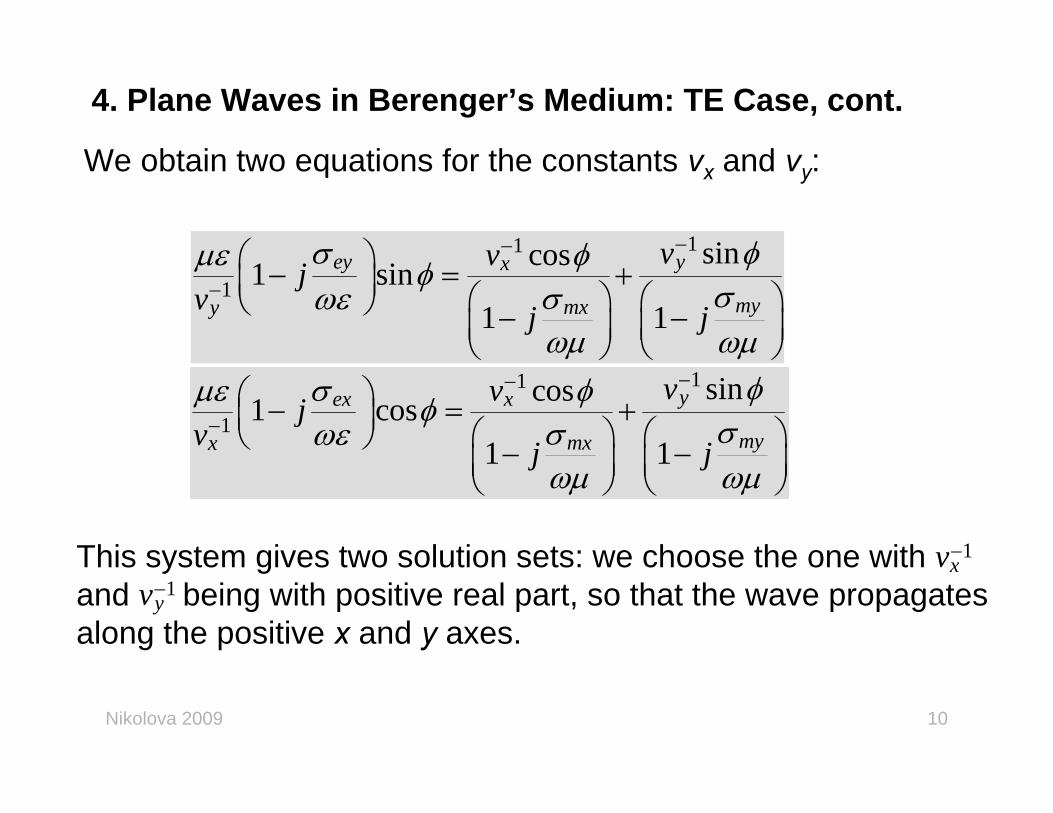
4. Plane Waves in Berenger’s Medium: TE Case, cont.

11

1sincos1 sin

1 1

ey yx

mymxy

vvjv j j

σ φμε φφσσωε

ωμ ωμ

−−

−⎛ ⎞− = +⎜ ⎟ ⎛ ⎞ ⎛ ⎞⎝ ⎠ − −⎜ ⎟ ⎜ ⎟

⎝ ⎠ ⎝ ⎠

We obtain two equations for the constants vx and vy:

11

1sincos1 cos

1 1

yex x

mymxx

vvjv j j

φμε σ φφσσωε

ωμ ωμ

−−

−⎛ ⎞− = +⎜ ⎟ ⎛ ⎞ ⎛ ⎞⎝ ⎠ − −⎜ ⎟ ⎜ ⎟

⎝ ⎠ ⎝ ⎠

This system gives two solution sets: we choose the one with and being with positive real part, so that the wave propagates along the positive x and y axes.

1xv−

1yv−

Nikolova 2009 11

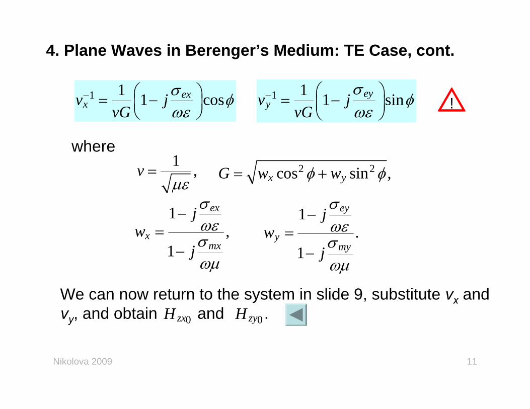
4. Plane Waves in Berenger’s Medium: TE Case, cont.

1 1 1 cosexxv j

vGσ φωε

− ⎛ ⎞= −⎜ ⎟⎝ ⎠

1 1 1 sineyyv j

vGσ

φωε

− ⎛ ⎞= −⎜ ⎟⎝ ⎠

1 ,vμε

= 2 2cos sin ,x yG w wφ φ= +

where

1,

1

ex

xmx

jw

j

σωεσωμ

−=

−

1.

1

ey

ymy

jw

j

σωεσωμ

−=

−

We can now return to the system in slide 9, substitute vx and vy, and obtain and .0zxH 0zyH

!

Nikolova 2009 12

4. Plane Waves in Berenger’s Medium: TE Case, cont.

2

00cosx

zxwH E

Gφ

η=

2

00siny

zyw

H EG

φη

= μηε

=

0 00 0z zx zyGH H H Eη

⇒ = + =

Thus, the intrinsic impedance of the wave in Berenger’s PML medium is

0

0PML

z

EH G

ηη = = !

Nikolova 2009 13

4. Plane Waves in Berenger’s Medium: TE Case, cont.

Each of the wave components is of the form

01exp( ) exp 1 cos

1 exp 1 sin .

ex

ey

j t j j xvG

j j yvG

σψ ψ ω ω φωεσ

ω φωε

⎡ ⎤⎛ ⎞= ⋅ − ⋅ − ⋅ ×⎜ ⎟⎢ ⎥⎝ ⎠⎣ ⎦⎡ ⎤⎛ ⎞− ⋅ − ⋅⎜ ⎟⎢ ⎥⎝ ⎠⎣ ⎦

0cos sinexp exp cos

exp sin

ex

ey

x yj t xvG G

yG

φ φ ηψ ψ ω σ φ

η σ φ

+⎡ ⎤⎛ ⎞ ⎛ ⎞= − ⋅ − ⋅ ×⎜ ⎟ ⎜ ⎟⎢ ⎥⎝ ⎠ ⎝ ⎠⎣ ⎦⎛ ⎞− ⋅⎜ ⎟⎝ ⎠

Re-arranging:

1xv−

1yv−

Nikolova 2009 14

5. Impedance Match at the Interface with PMLIf the conditions

are fulfilled, then

, ey myex mx σ σσ σε μ ε μ

= = !

2 2cos sin 1x yG w wφ φ⇒ = + =1x yw w= =

PMLη η⇒ =

The last equation shows that the impedance of the PML medium is equal to that of the loss-free medium regardless of the angle of propagation: impedance match is achieved for plane waves of any angle of incidence.

Nikolova 2009 15

5. Impedance Match at the Interface with PML, cont.The wave in the PML propagates as

( )2

0

attenuationphase delay: ( ) ( )/

cos sinexp exp cos sinex ey

j t j tv

x yj t x yv

ω ω

φ φψ ψ ω η σ φ σ φ

− = − ⋅⋅

+⎡ ⎤⎛ ⎞= − ⋅ − ⋅ + ⋅⎡ ⎤⎜ ⎟ ⎣ ⎦⎢ ⎥⎝ ⎠⎣ ⎦r v k r

( cos sin ),ˆ ˆv φ φ= +v x y

E

x

y

zˆ zH=H z

φ P

φv

x

y

z

r

φvxv

yv /( ˆ)ˆfrontv v= ⋅v r

retardation time is

2

( ˆ)ˆ

ˆ front

v

r rv v

v

τ

⋅

⋅= =

⋅= =

v r

r vr v

v vω⎛ ⎞= ⎜ ⎟⎝ ⎠

vk

Nikolova 2009 16

5. Impedance Match at the Interface with PML, cont.We now have to ensure that the continuity of the tangential field components is achieved by matching their phase terms along the axis tangential to the boundary. Assume that the boundary is along the y-axis (unit normal is x). Then, the matching of the phase terms at the interface along y requires (see slide 13 or 15)

This can be achieved only if , which in accordance with the impedance-match condition means also that . There will be no attenuation along the tangential y-axis.

0eyσ =0myσ =

On the other hand, we require maximum attenuation along the x-axis. We choose appropriate functions for and ( )ex xσ ( )mx xσwhich satisfy the impedance-match condition.

( )exp sin exp 1 sineyj y j j yσ

ω με φ ω με φωε

⎡ ⎤⎛ ⎞− ⋅ = − − ⋅⎜ ⎟⎢ ⎥⎝ ⎠⎣ ⎦at 0x =

Nikolova 2009 17

6. Berenger 2-D PML: TEz Case

x

y

z

(1) (1)PML(0,0; , )ey myσ σ

(2) (2)PML(0,0; , )ey myσ σ

(2)(2)

PML(

,;0,0)

exm

xσ

σ

(1)

(1)

PML(

,;0

,0)

exm

xσ

σ

(2) (2) (2) (2)PML( , ; , )ex mx ey myσ σ σ σ(1) (1) (2) (2)PML( , ; , )ex mx ey myσ σ σ σ

(2) (2) (1) (1)PML( , ; , )ex mx ey myσ σ σ σ

(1) (1) (1) (1)PML( , ; , )ex mx ey myσ σ σ σ

Nikolova 2009 18

6. Berenger 2-D PML: TEz Case, cont.

When a PML interface is orthogonal to the x axis (its unit normal is along x), the wave components must attenuate along x. This is accomplished by introducing σex and σmx. To ensure the continuity of the tangential field components, σey and σmymust be zero.

On the contrary, for an interface of unit vector along y, nonzero σey and σmy are introduced, while σex and σmx are zero.

At corner regions, all four loss parameters are nonzero.

Nikolova 2009 19

7. Berenger 2-D PML: TMz Case

The analysis for the TE case can be repeated for a TMz wave, and it follows along the same lines. The results are dual. We give a summary below.

The split equations for the TMz case are

xx

yze zx

HE Ext

ε σ∂∂

=∂ ∂

+( )zx zyx

m xyE EH H

t yμ σ

∂ +∂+ = −

∂∂

( )y zx zym yx

H Ex

EH

tμ σ∂ ∂ +

+ =∂∂

yy

z xe zy

E HEyt

ε σ∂ ∂

+ = −∂∂

The PML matching conditions are the same and the 2-D PML regions are constructed as in slide 17.

Nikolova 2009 20

8. Berenger’s 3-D PMLIn 3-D, all six field components are split according to the field component derivatives generating them. The procedure of splitting is identical to the 2-D cases.

( )x zx zyyey E Hy

Ht

ε σ∂ ∂⎛ ⎞+ = +⎜ ⎟∂ ∂⎝ ⎠

( )x yx yzzez E Hz

Ht

ε σ∂ ∂⎛ ⎞+ = − +⎜ ⎟∂ ∂⎝ ⎠

( )y xy xzzez E Hz

Ht

ε σ∂ ∂⎛ ⎞+ = +⎜ ⎟∂ ∂⎝ ⎠

( )y zx zyxex E Hx

Ht

ε σ∂ ∂⎛ ⎞+ = − +⎜ ⎟∂ ∂⎝ ⎠

( )z yx yzxex E Hx

Ht

ε σ∂ ∂⎛ ⎞+ = +⎜ ⎟∂ ∂⎝ ⎠

( )z xy xzyey E Hy

Ht

ε σ∂ ∂⎛ ⎞+ = − +⎜ ⎟∂ ∂⎝ ⎠

( )x zx zyymy H Ey

Et

μ σ∂ ∂⎛ ⎞+ = − +⎜ ⎟∂ ∂⎝ ⎠

( )x yx yzzmz H Ez

Et

μ σ∂ ∂⎛ ⎞+ = +⎜ ⎟∂ ∂⎝ ⎠

( )y zx zyxmx H Ex

Et

μ σ∂ ∂⎛ ⎞+ = +⎜ ⎟∂ ∂⎝ ⎠

( )y xy xzzmz H Ez

Et

μ σ∂ ∂⎛ ⎞+ = − +⎜ ⎟∂ ∂⎝ ⎠

( )z yx yzxmx H Ex

Et

μ σ∂ ∂⎛ ⎞+ = − +⎜ ⎟∂ ∂⎝ ⎠

( )z xy xzymy H Ey

Et

μ σ∂ ∂⎛ ⎞+ = +⎜ ⎟∂ ∂⎝ ⎠

Nikolova 2009 21

8. Berenger’s 3-D PML, cont.The matching conditions at a planar interface between the loss-free computational region and the PML require that the specific conductivities along the unit normal of the interface must be nonzero and satisfying the impedance-match condition

en mnσ σε μ

=

where n denotes the axis orthogonal to the planar interface. The other two pairs of conductivities (along the axes which are tangential to the interface) are set equal to zero.

In a dihedral corner where two orthogonal PMLs overlap, two pairs of conductivities are nonzero – the ones which are nonzero in the neighboring PMLs.In a trihedral corner where three PMLs overlap, all six conductivities must be nonzero.

Nikolova 2009 22

8. Berenger’s 3-D PML, cont.

xyz

, 00

ey my

ex mx ez mz

σ σσ σ σ σ

≠= = = =

, , , 00

ey my ez mz

ex mx

σ σ σ σσ σ

≠= =

, 0, 0, 0

ey my

ez mz

ex mx

σ σσ σσ σ

≠≠≠

Nikolova 2009 23

8. Berenger’s 3-D PML, cont.

Discrete form of the PML equations (example for the Exy, Hxy):

( )x zx zyyey E Hy

Ht

ε σ∂ ∂⎛ ⎞+ = +⎜ ⎟∂ ∂⎝ ⎠

, , , 1,, , , ,

0.5 0.51

, ,i j k i j k

i j k i j k

n nz zn E n E

E j H jxy xy

H HE k E k

y−

+ ++

−⎛ ⎞= ⋅ + ⋅⎜ ⎟⎜ ⎟Δ⎝ ⎠

( )x zx zyymy H Ey

Et

μ σ∂ ∂⎛ ⎞+ = − +⎜ ⎟∂ ∂⎝ ⎠

, 1, , ,, , , ,0.5 0.5

, ,i j k i j k

i j k i j k

n nz zn H n H

H j E jxy xy

E EH k H k

y++ −

−⎛ ⎞= − ⋅⎜ ⎟⎜ ⎟Δ⎝ ⎠

,, ,

, ,

1 /, ,1 1

e jE EE j H j

e j e j

tk kξ εξ ξ

− Δ= =

+ +

,, ,

, ,

1 /, ,1 1

m jH HH j E j

m j m j

tk kξ μξ ξ

− Δ= =

+ +

,, 2

ey je

yj

j y

tσξ

ε = Δ

Δ=

,

),

( 1/22m

y j

y jm j

y

tσξ

μ = + Δ

Δ=

ˆ ˆ=n y

Nikolova 2009 24

8. Berenger’s 3-D PML, cont.Discrete form of the PML equations as first proposed by Berenger, exponential time stepping (example for the Exy, Hxy):

( )x zx zyyey E Hy

Ht

ε σ∂ ∂⎛ ⎞+ = +⎜ ⎟∂ ∂⎝ ⎠

( ), , , , , , , 1,1 0.5 0.5

, ,i j k i j k i j k i j kn E n E n n

E j H jxy xy z zE k E k H H−

+ + += ⋅ + ⋅ −

( )x zx zyymy H Ey

Et

μ σ∂ ∂⎛ ⎞+ = − +⎜ ⎟∂ ∂⎝ ⎠

( ), , , , , 1, , ,0.5 0.5

, ,i j k i j k i j k i j kn H n H n n

H j E jxy xy z zH k H k E E+

+ −= − ⋅ −

/ ,,, ,

1,

Et E jE Eey j

E j H jey

kk e k

yσ ε

σ− Δ −

= =Δ

/ ,,, ,

1,

Ht H jH Hmy j

H j E jmy

kk e k

yσ μ

σ− Δ −

= =Δ

Nikolova 2009 25

9. PML Loss ParametersTheoretical reflection from the PMLThe PML is usually backed by a PEC wall. The reflected signal undergoes reflection at the PML termination but also undergoes substantial attenuation corresponding to double the thickness of the PML d. In a PML layer where constant attenuation is assumed along the normal direction only (the tangential conductivities are zero), the reflection coefficient becomes

( )( ) exp 2 cosenR dφ σ η φ= − ⋅

d

φn̂

0cos sin( , ) expexp( cos )ex

x yxx y j tv

φ φψ φ ωσψ η +⎡ ⎤⎛ ⎞= ⋅ ⋅− −⎜ ⎟⎢ ⎥⎝ ⎠⎣ ⎦⋅

Reminder (see slide 15): If n = x, then

Nikolova 2009 26

9. PML Loss Parameters, cont.

R(Φ) is the PML reflection error. It gives the relative magnitude of the spurious reflected wave, which enters back into the computational domain. The larger d and σen are, the less the reflection. However, the angle of incidence Φ plays an important role, too. When Φ = 90 deg., R = 1! At grazing angles of incidence, the PML is ineffective at the corner regions of the computational domain.

In practice, the Berenger PML is placed sufficiently far from sources and guiding structures so that the plane-wave components of the field impinge upon the interface at angles smaller than 90 deg.

Nikolova 2009 27

9. PML Loss Parameters, cont.PML in Discrete Space

Theoretically, reflectionless wave transmission should take place through the PML interface, regardless of the local step discontinuity in the normal conductivities σen and σmn. In practice, however, spurious numerical reflections do arise, because of thefinite spatial sampling of the field. Therefore, we can not set σenand σmn to be large constant numbers throughout the PML.

The conductivities are made functions of the PML depth: they have to be very small close to the PML interface (in order to ensure as little as possible spurious reflection), and then increase as quickly as possible toward the PEC termination wall (in order to ensure sufficient attenuation).

Nikolova 2009 28

9. PML Loss Parameters, cont.Assume that x is the position measured from the PML interface inward toward its PEC termination. Then, for ( )ex xσ

0

( ) exp 2 cos ( )d

enR x dxφ η φ σ⎛ ⎞

= − ⋅⎜ ⎟⎜ ⎟⎝ ⎠

∫

There are various profiles for the conductivity.

(a) Polynomial grading

max

m

ex exd

σ σ⎛ ⎞= ⎜ ⎟⎝ ⎠

max(0) 0, ( )ex ex edσ σ σ⇒ = =

The bigger m is, the smoother the change of σex close to theinterface. But, then, the steeper its slope is close to the PEC walls: spurious numerical reflections occur deeper in the PML.

Nikolova 2009 29

9. PML Loss Parameters, cont.We then have to bring down σe,max. This, however, may lead to insufficient attenuation. Alternatively, we can keep σe,maxlarge but increase the PML depth d to allow for acceptable slopes at all points deep in the PML. This, however, means increase of the required computational resources.

Designing an efficient PML is not an easy task!

Typical optimal values:

The reflection coefficient with polynomial grading is

[ ]max( ) exp 2 cos /( 1)eR d mφ ησ φ= − +

16 8(0) 10 (for 10 ), 10 (for 5 )R d x d x− −≈ = Δ = Δ

2 6m≤ ≤

Nikolova 2009 30

9. PML Loss Parameters, cont.When R(0), m, and d are set, we can compute σe,max:

[ ]max

( 1) ln (0)2e

m Rd

ση

+= −

(a) Geometric gradingThe PML loss factor is defined as

( )1/0( )

xxex xx gσ σΔ=

scaling factor conductivity at interface

( )/0( ) exp 2 1 cos / lnd x

xR x g gφ ησ φΔ⎡ ⎤⇒ = − Δ −⎣ ⎦

/0 0(0) , ( ) d x

ex x ex xd gσ σ σ σ Δ⇒ = =

Nikolova 2009 31

9. PML Loss Parameters, cont.

σx0 must be small for less spurious reflection from the interface. The scaling g > 1 determines the rate of increase of the conductivity. Large g’s flatten the conductivity profile near the interface and make it steeper deeper into the PML. Usually,

2 3g≤ ≤

If R(0), g and d are given, we can compute σx0:

[ ]( )0 /

ln (0) ln2 1x d x

R gx g

ση Δ

= −Δ −

Nikolova 2009 32

9. PML Loss Parameters, cont.

There is another implementational detail concerning the computation of the conductivity at a mesh point: it is given by the average value in the cell around the index (L) location:

( 0.5)

( 0.5)

1( ) ( )L x

en enL x

L x dxx

σ σ+ Δ

− Δ

=Δ ∫

Thus, for a polynomial grading of order m in a PML, which is N-cell thick,

[ ]max( , )1 2 1

ln (0)(0)

( 1)2 2em N

ex m m m mR

m N xNσσ

η+ + += = −+ Δ

( , ) ( , ) 1 1( 0) (0) (2 1) (2 1)m N m N m mex exL L Lσ σ + +⎡ ⎤> = ⋅ + − −⎣ ⎦

Nikolova 2009 33

9. PML Loss Parameters, cont.For the geometric grading of scaling g in a PML of N cells,

[ ]( , )0

(1 ) ln (0)1(0)ln 2 ( 1)

g Nex e N

g Rgg x g

σ ση−−

= =Δ −

( , ) ( , ) 1/ 2( 0) (0)g N g N Lex exL gσ σ −> = ⋅

Nikolova 2009 34

Important topics not mentioned in this courseFDTD numerical dispersion errors

FDTD on curvilinear grids, conformal FDTD (C-FDTD) schemes

FDTD in dispersive and anisotropic media

FDTD in nonlinear and gain materials

Integrating lumped elements with the FDTD full-wave analysis

Excitation schemes for enhanced convergence

Near-to-Far-Field transformation for antenna radiation patterns

Modified implicit FDTD schemes – the FDTD-ADI

Eigen-mode analysis of waveguides

S-parameter analysis with FDTD