finite element simulation and assessment … single-degree-of-freedom prediction methodology for...
TRANSCRIPT
AFRL-RX-TY-TR-2011-0031
FINITE ELEMENT SIMULATION AND ASSESSMENT OF SINGLE-DEGREE-OF-FREEDOM PREDICTION METHODOLOGY FOR INSULATED CONCRETE SANDWICH PANELS SUBJECTED TO BLAST LOADS
James S. Davidson Department of Civil Engineering Auburn University 238 Harbert Engineering Center Auburn, AL 36849 Charles M. Newberry Jacobs ASG 1020 Titan Court Fort Walton Beach, FL 32547 Michael I. Hammons and Bryan T. Bewick Air Force Research Laboratory 139 Barnes Drive, Suite 2 Tyndall Air Force Base, FL 32403-5323 Contract No. FA4819-09-C-0032 February 2011
AIR FORCE RESEARCH LABORATORY MATERIALS AND MANUFACTURING DIRECTORATE
Air Force Materiel Command
United States Air Force Tyndall Air Force Base, FL 32403-5323
DISTRIBUTION A: Approved for public release; distribution unlimited.

DISCLAIMER
Reference herein to any specific commercial product, process, or service by trade name,
trademark, manufacturer, or otherwise does not constitute or imply its endorsement,
recommendation, or approval by the United States Air Force. The views and opinions of
authors expressed herein do not necessarily state or reflect those of the United States Air
Force.
This report was prepared as an account of work sponsored by the United States Air Force.
Neither the United States Air Force, nor any of its employees, makes any warranty,
expressed or implied, or assumes any legal liability or responsibility for the accuracy,
completeness, or usefulness of any information, apparatus, product, or process disclosed, or
represents that its use would not infringe privately owned rights.


Standard Form 298 (Rev. 8/98)
REPORT DOCUMENTATION PAGE
Prescribed by ANSI Std. Z39.18
Form Approved OMB No. 0704-0188
The public reporting burden for this collection of information is estimated to average 1 hour per response, including the time for reviewing instructions, searching existing data sources, gathering and maintaining the data needed, and completing and reviewing the collection of information. Send comments regarding this burden estimate or any other aspect of this collection of information, including suggestions for reducing the burden, to Department of Defense, Washington Headquarters Services, Directorate for Information Operations and Reports (0704-0188), 1215 Jefferson Davis Highway, Suite 1204, Arlington, VA 22202-4302. Respondents should be aware that notwithstanding any other provision of law, no person shall be subject to any penalty for failing to comply with a collection of information if it does not display a currently valid OMB control number. PLEASE DO NOT RETURN YOUR FORM TO THE ABOVE ADDRESS. 1. REPORT DATE (DD-MM-YYYY) 2. REPORT TYPE 3. DATES COVERED (From - To)
4. TITLE AND SUBTITLE 5a. CONTRACT NUMBER
5b. GRANT NUMBER
5c. PROGRAM ELEMENT NUMBER
5d. PROJECT NUMBER
5e. TASK NUMBER
5f. WORK UNIT NUMBER
6. AUTHOR(S)
7. PERFORMING ORGANIZATION NAME(S) AND ADDRESS(ES) 8. PERFORMING ORGANIZATION REPORT NUMBER
9. SPONSORING/MONITORING AGENCY NAME(S) AND ADDRESS(ES) 10. SPONSOR/MONITOR'S ACRONYM(S)
11. SPONSOR/MONITOR'S REPORT NUMBER(S)
12. DISTRIBUTION/AVAILABILITY STATEMENT
13. SUPPLEMENTARY NOTES
14. ABSTRACT
15. SUBJECT TERMS
16. SECURITY CLASSIFICATION OF: a. REPORT b. ABSTRACT c. THIS PAGE
17. LIMITATION OF ABSTRACT
18. NUMBER OF PAGES
19a. NAME OF RESPONSIBLE PERSON
19b. TELEPHONE NUMBER (Include area code)
01-FEB-2011 Interim Technical Report 01-MAY-2009--31-DEC-2010
Finite Element Simulation and Assessment of Single-Degree-of-Freedom Prediction Methodology for Insulated Concrete Sandwich Panels Subjected to Blast Loads
FA4819-09-C-0032
0602102F
4918
C1
QF101013
*Davidson, James S.; **Newberry, Charles M.; #Hammons, Michael I.; #Bewick, Bryan T.
*Department of Civil Engineering, Auburn University, 238 Harbert Engineering Center, Auburn, AL 36849; **Jacobs ASG, 1020 Titan Court, Fort Walton Beach, FL 32547
#Air Force Research Laboratory Materials and Manufacturing Directorate Airbase Technologies Division 139 Barnes Drive, Suite 2 Tyndall Air Force Base, FL 32403-5323
AFRL/RXQEM
AFRL-RX-TY-TR-2011-0031
Distribution Statement A: Approved for public release; distribution unlimited.
Ref Public Affairs Case # 88ABW-2012-0180, 10 January 2012. Document contains color images.
This report discusses simulation methodologies used to analyze large deflection static and dynamic behavior of foam-insulated concrete sandwich wall panels. Both conventionally reinforced cast-on-site panels and precast/prestressed panels were considered. The experimental program used for model development and validation involved component-level testing as well as both static and dynamic testing of full-scale wall panels. The static experiments involved single spans and double spans subjected to near-uniform distributed loading. The dynamic tests involved spans up to 30 ft tall that were subjected to impulse loads generated by an external explosion. Primary modeling challenges included: (1) accurately simulating prestressing initial conditions in an explicit dynamic code framework, (2) simulating the concrete, reinforcement, and foam insulation in the high strain rate environment, and (3) simulating shear transfer between wythes, including frictional slippage and connector rupture. Correlation challenges, conclusions and recommendations regarding efficient and accurate modeling techniques are highlighted. The modeling methodologies developed were used to conduct additional behavioral studies and help to assess single-degree-of-freedom prediction methodology developed for foam-insulated precast/prestressed sandwich panels for blast loads.
blast load; finite element modeling; large deflection behavior; load-deflection response; precast concrete; prestressed concrete; sandwich panel
U U U UU 87
Christopher L. Genelin
Reset

i Distribution Statement A: Approved for public release; distribution unlimited.
TABLE OF CONTENTS
LIST OF FIGURES ....................................................................................................................... iii LIST OF TABLES ......................................................................................................................... vi ABSTRACT .................................................................................................................................. vii ACKNOWLEDGMENTS ........................................................................................................... viii 1. INTRODUCTION ...............................................................................................................1 1.1. Overview ..............................................................................................................................1 1.2. Objectives ............................................................................................................................1 1.3. Scope and Methodology ......................................................................................................1 1.4. Report Organization .............................................................................................................2 2. TECHNICAL BACKGROUND ..........................................................................................3 2.1. Overview ..............................................................................................................................3 2.2. Blast Loading .......................................................................................................................3 2.3. Precast/Prestressed Sandwich Wall Panels ..........................................................................4 2.4. Design of Precast/Prestressed Concrete Structures for Blast ...............................................6 3. MODEL DEVELOPMENT AND VALIDATION .............................................................7 3.1. Overview ..............................................................................................................................7 3.2. Reinforced Concrete Beam Validation ................................................................................7 3.2.1. Concrete Model and Parameters ..........................................................................................8 3.2.2. Mechanical Behavior and Concrete Plasticity .....................................................................9 3.2.3. Yield Function ...................................................................................................................12 3.2.4. Material Parameters of Concrete Damage Plasticity Model ..............................................14 3.2.5. Reinforcements (Rebar and Welded Wire Reinforcement) ...............................................14 3.2.6. Geometry, Elements, Loading, and Boundary Conditions ................................................16 3.2.7. Nonlinear Incremental Analysis ........................................................................................16 3.2.8. Static RC Flexure Test and FE Results Comparison .........................................................17 3.3. Static Tests of Sandwich Panels ........................................................................................17 3.3.1. Shear Connectors ...............................................................................................................18 3.3.2. Static Shear Tie Tests.........................................................................................................19 3.3.3. Shear Tie Modeling Methodology .....................................................................................19 3.3.4. Implementation of the MPC Approach into Sandwich Panel Models ...............................21 3.3.5. Simulation of Prestressing Effects in Sandwich Panel Models .........................................22 3.3.6. Insulation Foam Modeling .................................................................................................23 3.3.7. Static Sandwich Panel Tests and Modeling Comparisons .................................................26 3.4. Dynamic Modeling and Experimental Comparisons .........................................................26 3.4.1. Full-scale Dynamic Tests ...................................................................................................28 3.4.2. Dynamic Finite Element Models .......................................................................................31 3.4.3. Simulation of Prestressing Effects in LS-DYNA ..............................................................31 3.4.4. Simulation of Dynamic Increase Factors ...........................................................................31 3.4.5. Dynamic Sandwich Panel Experiment and FE Model Comparisons .................................32 3.4.6. Single Span Results and Comparisons ...............................................................................32 3.4.7. Multi-span Results and Comparisons ................................................................................35 4. STUDY OF BLAST RESPONSE BEHAVIOR OF SANDWICH PANELS ...................41 4.1. Introduction ........................................................................................................................41 4.2. Energy Dissipation .............................................................................................................41 4.3. Strain Distribution ..............................................................................................................42

ii Distribution Statement A: Approved for public release; distribution unlimited.
4.4. Reaction Force vs. FE Models ...........................................................................................45 5. SINGLE-DEGREE-OF-FREEDOM (SDOF) MODEL DEVELOPMENT ......................48 5.1. Introduction ........................................................................................................................48 5.2. General SDOF Methodology .............................................................................................48 5.3. Development of Sandwich Panel SDOF Prediction Models .............................................52 5.3.1. Static Resistance of Sandwich Panels and SDOF Models .................................................52 5.3.2. Correlation with Current Prediction Methods....................................................................53 5.3.3. Resistance Calculation .......................................................................................................53 5.3.4. Material Dynamic Properties Calculation ..........................................................................54 5.4. SDOF Prediction Model Comparisons ..............................................................................57 5.4.1. SDOF Prediction Model Matrix.........................................................................................57 5.4.2. SDOF Prediction Model Comparisons – Dynamic Series I...............................................58 5.4.3. SDOF Prediction Model Comparisons – Dynamic Series II .............................................60 5.4.4. Resistance and Energy Comparisons .................................................................................62 5.4.5. SDOF Prediction Model Comparisons – FE Modeling .....................................................69 6. CONCLUSIONS AND RECOMMENDATIONS ............................................................73 6.1. Conclusions ........................................................................................................................73 6.2. Recommendations ..............................................................................................................74 7. REFERENCES ..................................................................................................................75 LIST OF SYMBOLS, ABBREVIATIONS, AND ACRONYMS ................................................77

iii Distribution Statement A: Approved for public release; distribution unlimited.
LIST OF FIGURES
Page Figure 1. Pressure vs. Time Description for Arbitrary Explosion ...................................................4 Figure 2. Organizational Chart of Model Development ..................................................................7 Figure 3. University of Missouri Loading-tree Apparatus Setup and Reinforced Beam
Validation Sample ................................................................................................................8 Figure 4. Layout of Reinforced Concrete Beam Specimens............................................................9 Figure 5. Response of Concrete to Uniaxial Loading in (a) Tension and (b) Compression
(ABAQUS, 2008) ..............................................................................................................12 Figure 6. Yield Surfaces in the Deviatoric Plane, Corresponding to Different values of Kc
(ABAQUS, 2008) ..............................................................................................................13 Figure 7. Stress-Strain Relationship of Rebar Used in the Analyses .............................................15 Figure 8. Stress-Strain Relationship of WWR Used in the Analyses ............................................15 Figure 9. FE Models: (a) Loading and Boundary Conditions and (b) Concrete, Rebar and
WWR Elements .................................................................................................................16 Figure 10. RC Beam Design 1 vs. FEA (left), RC Beam Design 2 vs. FEA (right) ......................17 Figure 11. Conventionally Reinforced 3-2-3 Static Sandwich Panel Specimen ...........................18 Figure 12. Shear Tie Static Test Configuration (Naito, et al. 2009a) ............................................19 Figure 13. Shear Tie MPC Validation Model Configuration ........................................................20 Figure 14. Validation of MPC Approach Composite Shear Tie (top) Non-composite Shear
Tie (bottom) .......................................................................................................................20 Figure 15. Generalized Shear Tie Resistances Used in the MPC Approach: (a) Composite
Carbon; (b) Composite Fiberglass; (c) Non-composite Fiberglass....................................21 Figure 16. FE Model of Sandwich Panel Utilizing MPC for Shear Tie Behavior .........................22 Figure 17. Stress-Strain Relationship of Prestressing Strand Used in the Analyses .....................23 Figure 18. Comparison of Stress-Strain Response of Various Extruded Polystyrene Products
(Jenkins, 2008) ...................................................................................................................23 Figure 19. Comparison of Similar Panel Resistances with Different Foam Insulation .................24 Figure 20. Test Setup for Static Testing of Insulation Foam Materials .........................................24 Figure 21. Stress-Strain Curve of Expanded Polystyrene Insulation Foam Samples ....................25 Figure 22. Stress-Strain Curve of Polyisocyanruate Insulation Foam Samples ............................25 Figure 23. Stress-Strain Curve of Extruded Expanded Polystyrene Insulation Foam Samples ....26 Figure 24. Static Test Results vs Finite Element Model Comparisons..........................................28 Figure 25. Test Setup for Full Scale Dynamic Tests with Single Span Reaction Structure
(left) and Multi-span Reaction Structure (right) (Naito et all., 2010b) ..............................29 Figure 26. (a) Average Primary Detonation Reflected Pressure Curves Both Experiments and
Reactions Structures (b) Average Impulse Curves Associated with the Average Reflected Pressure Curves .................................................................................................30
Figure 27. LS-DYNA Default Curve for Concrete DIF ................................................................32 Figure 28. Experiment 1–Primary Detonation Measured Midspan Displacement vs. Finite
Element Displacement Comparison for (a) SS1, (b) SS2, (c), SS3, (d) SS4 .....................33 Figure 29. Experiment 2–Primary Detonation Measured Midspan Displacement vs. Finite
Element Midspan Displacement Comparison for (a) SS1, (b) SS2, (c) SS3, (d) SS4 .......33 Figure 30. Pre-detonation Pressure and Impulse for Single Span Reaction Structure–
Experiment 1 ......................................................................................................................34

iv Distribution Statement A: Approved for public release; distribution unlimited.
Figure 31. Experiment 1–Pre-detonation Measured Midspan Displacement vs. Finite Element Midspan Displacement Comparison for (a) SS1, (b) SS2, (c) SS3, (d) SS4 .....................35
Figure 32. Experiment 1–Primary Detonation Measured First Floor Midspan Displacement vs. Finite Element Midspan Displacement Comparison for (a) MS1, (b) MS2, (c) MS3, (d) MS4 ...................................................................................................................36
Figure 33. Experiment 1– Primary Detonation Measured Second Floor Midspan Displacement vs. Finite Element Midspan Displacement Comparison for (a) MS1, (b) MS2, (c) MS3, (d) MS4 .....................................................................................................36
Figure 34. Experiment 2– Primary Detonation Measured First Floor Midspan Displacement vs. Finite Element Midspan Displacement Comparison for (a) MS1, (b) MS2, (c) MS3, (d) MS4 ....................................................................................................................37
Figure 35. Primary Detonation Measured Second Floor Midspan Displacement vs. Finite Element Midspan Displacement Comparison for (a) MS2, (b) MS3, (c) MS4 .................37
Figure 36. Localized Effects Along the Second Floor Support .....................................................38 Figure 37. Pre-detonation Pressure and Impulse for Multi-span Reactions Structure–
Experiment 1 ......................................................................................................................38 Figure 38. Experiment 1– Pre-detonation Measured First Floor Midspan Displacement vs.
Finite Element Midspan Displacement Comparison for (a) MS1, (b) MS2, (c) MS3, (d) MS4 ..............................................................................................................................39
Figure 39. Pre-detonation Measured Second Floor Midspan Displacement vs. Finite Element Midspan Displacement Comparison for (a) MS1, (b) MS2, (c) MS3, (d) MS4 ................39
Figure 40. Second Floor Support Frame Allowing Interaction Between the Behaviors of All Multi-span Panels Attached ...............................................................................................40
Figure 41. Kinetic Energy of Sandwich Panel System Components–Experiment 1; (a) SS1, (b) SS2, (c) SS3, (d) SS4 ...................................................................................................42
Figure 42. SS1–Experiment 1: Strain of Reinforcement of Interior Concrete Wythe Across Panel Height Over Time ....................................................................................................43
Figure 43. SS3–Experiment 1: Strain of Reinforcement of Interior Concrete Wythe Across Panel Height Over Time ....................................................................................................43
Figure 44. SS4–Experiment 1: Strain of Reinforcement of Interior Concrete Wythe Across Panel Height Over Time ....................................................................................................44
Figure 45. Average Pressure for Experiment 1 Used for Finite Element Models Simulating Single Span Test Specimens ..............................................................................................44
Figure 46. Load Cells Recording Reaction Force for Single Span Specimens .............................45 Figure 47. Comparison of Measured Total Reaction Force and Recorded FE Model Reaction
Forces for Experiment 1–SS1 ............................................................................................46 Figure 48. Comparison of Measured Total Reaction Force and Recorded FE Model Reaction
Forces for Experiment 1–SS2 ............................................................................................46 Figure 49. Comparison of Measured Total Reaction Force and Recorded FE Model Reaction
Forces for Experiment 1–SS3 ............................................................................................47 Figure 50. Comparison of Measured Total Reaction Force and Recorded FE Model Reaction
Forces for Experiment 1–SS4 ............................................................................................47 Figure 51. (a) Displacement Representation of Sandwich Panel Subjected to Blast Load (b)
Equivalent Single-Degree-of-Freedom System .................................................................50 Figure 52. Screenshot of SDOF Model in Spreadsheet Format .....................................................52 Figure 53. Comparison of Experimental Resistance to Bilinear Resistance Curve .......................53

v Distribution Statement A: Approved for public release; distribution unlimited.
Figure 54. Screenshots of Developed SDOF Prediction Analysis Spreadsheet Resistance Input ...................................................................................................................................54
Figure 55. Coefficients of Cracked Moment of Inertia (UFC 2-340-02) ......................................57 Figure 56. Dynamic Series I, Detonation 2 Measured Displacement Comparison to SDOF
Prediction Using Weighted Resistance ..............................................................................59 Figure 57. Dynamic Series I, Detonation 3 Measured Displacement Comparison to SDOF
Prediction Using Weighted Resistance ..............................................................................60 Figure 58. Evaluation of Weighted Resistance Prediction Method vs. Measured Data:
Dynamic Series II–Experiment 1 (a) SS1 (b) SS2 (c) SS3 (d) SS4 ...................................61 Figure 59. Evaluation of Weighted Resistance Prediction Method vs. Measured Data:
Dynamic Series II–Experiment 2 (a) SS1 (b) SS2 (c) SS3 (d) SS4 ...................................62 Figure 60. Experiment 1 Loading: Predicted Response Comparisons of Weighted Resistance
SDOF and Experimental Resistance (a) SS1 (b) SS2 (c) SS3 (d) SS4 ..............................63 Figure 61. Experiment 2 Loading: Predicted Response Comparisons of Weighted Resistance
SDOF and Experimental Resistance (a) SS1 (b) SS2 (c) SS3 (d) SS4 ..............................64 Figure 62. Experiment 1 Loading: Resistance and Energy for SS1 ..............................................65 Figure 63. Experiment 1 Loading: Resistance and Energy for SS2 ..............................................65 Figure 64. Experiment 1 Loading: Resistance and Energy for SS3 ..............................................66 Figure 65. Experiment 1 Loading: Resistance and Energy for SS4 ..............................................66 Figure 66. Experiment 2 Loading: Resistance and Energy for SS1 ..............................................67 Figure 67. Experiment 2 Loading: Resistance and Energy for SS2 ..............................................67 Figure 68. Experiment 2 Loading: Resistance and Energy for SS3 ..............................................68 Figure 69. Experiment 2 Loading: Resistance and Energy for SS4 ..............................................68 Figure 70. Demonstration of Bilinear Resistance Impact on Conservative Response
Prediction ...........................................................................................................................69 Figure 71. FE Model Response vs. SDOF Prediction Using Weighted Resistance for (a) FE-
1, (b) FE-2, (c) FE-3, (d) FE-4 ...........................................................................................70 Figure 72. FE Model Response vs. SDOF Prediction Using Weighted Resistance for (a) FE-
5, (b) FE-6, (c) FE-7, (d) FE-8 ...........................................................................................71 Figure 73. FE Model Response vs. SDOF Prediction Using Weighted Resistance for (a) FE-
9, (b) FE-10, (c) FE-11, (d) FE-12 .....................................................................................72
vi Distribution Statement A: Approved for public release; distribution unlimited.
LIST OF TABLES
Page Table 1. Description of Reinforced Concrete Beam Samples .........................................................9 Table 2. Material Parameters of Concrete Damage Plasticity Model ............................................14 Table 3. Material Strengths for Reinforcements ............................................................................15 Table 4. Static Sandwich Panel Validation Matrix ........................................................................27 Table 5. Dynamic Test Specimen Details ......................................................................................30 Table 6. Primary Detonation Normalized Pressures and Impulses ................................................30 Table 7. Pre-detonation Comparison of Single Span Experimental and FE Model Natural
Period .................................................................................................................................34 Table 8. Pre-detonation Comparison of Multi-span Experimental and FE Model Natural
Period .................................................................................................................................40 Table 9. Dynamic Yield Strength for Conventional Reinforcement (USACE PDC, 2006) ..........55 Table 10. SDOF Prediction Model Comparison Matrix ................................................................58 Table 11. Percent Difference, Dynamic Series I SDOF Prediction vs. Measured Support
Rotation ..............................................................................................................................60 Table 12. Percent Difference, Dynamic Series II–Experiment 1 SDOF Prediction vs.
Measured Support Rotation ...............................................................................................61 Table 13. Percent Difference, Dynamic Series II–Experiment 2 SDOF Prediction vs.
Measured Support Rotation ...............................................................................................62 Table 14. Percent Difference, SDOF Prediction vs. FE Model Response .....................................70 Table 15. Percent Difference, SDOF Prediction vs. FE Model Response .....................................71 Table 16. Percent Difference, SDOF Prediction vs. FE Model Response .....................................72

vii Distribution Statement A: Approved for public release; distribution unlimited.
ABSTRACT
This report discusses simulation methodologies used to analyze large deflection static and dynamic behavior of foam-insulated concrete sandwich wall panels. Both conventionally reinforced cast-on-site panels and precast/prestressed panels were considered. The experimental program used for model development and validation involved component-level testing as well as both static and dynamic testing of full-scale wall panels. The static experiments involved single spans and double spans subjected to near-uniform distributed loading. The dynamic tests involved spans up to 30 ft tall that were subjected to impulse loads generated by an external explosion. Primary modeling challenges included: (1) accurately simulating prestressing initial conditions in an explicit dynamic code framework, (2) simulating the concrete, reinforcement, and foam insulation in the high strain rate environment, and (3) simulating shear transfer between wythes, including frictional slippage and connector rupture. Correlation challenges, conclusions and recommendations regarding efficient and accurate modeling techniques are highlighted. The modeling methodologies developed were used to conduct additional behavioral studies and help to assess single-degree-of-freedom prediction methodology developed for foam-insulated precast/prestressed sandwich panels for blast loads. Models showed that using a weighted bilinear resistance is a viable option in predicting behavior.

viii Distribution Statement A: Approved for public release; distribution unlimited.
ACKNOWLEDGMENTS
This work was sponsored in part by the Air Force Research Laboratory (AFRL) and a Daniel P. Jenny Research Fellowship Grant from the Precast/Prestressed Concrete Institute (PCI). The current technical points of contact for the AFRL Engineering Mechanics and Explosive Effects Group (EMEERG) are Drs. Michael Hammons and Bryan Bewick. The AFRL program manager during the experimental phase of the program was Dr. Robert Dinan. The static tests from which the model validation data was generated were conducted at the University of Missouri Remote Testing Facility under the direction of Professor Hani Salim. Professor Clay Naito of Lehigh University was the lead technical advisor of the AFRL/PCI test program. The dynamic tests in which the validation was based were conducted by the EMEERG, Airbase Technologies Division, of AFRL at Tyndall Air Force Base Florida. The AFRL test program was coordinated by John Hoemann, formally of Applied Research Associates, Inc., and now employed at the Engineer Research and Development Center, Vicksburg Mississippi. The test program also involved other employees of Applied Research Associates and Black & Veatch, Federal Services Division. Drs. Jim Davidson and Jun Kang at Auburn University provided finite element modeling technical guidance.

1 Distribution Statement A: Approved for public release; distribution unlimited.
1. INTRODUCTION
1.1. Overview
Threats to structures and the people residing within are increasing. Since the attacks on the World Trade Center and the Pentagon on September 11, 2001, the realization of such threats has promoted research in the field of structures subjected to impulse loads. The study of structures subjected to impulse loads has existed for decades; however, a shift in the type of risks structures face has occurred due to the more localized manner of current threats. Also, most of the criteria for designing structural components subjected to impulse loads were created before many modern concrete components were introduced. The behavior and design of structural components subjected to impulse loads differs from the behavior under static loads. Most loads such as wind and gravity loads are assumed to be static since the time in which they are applied is relatively large enough not to induce significant accelerations of structural components. Dynamic loads such as blasts last only a fraction of a second but may be quite large in magnitude and can induce significant accelerations and large displacements. The design of structural components for impulse loads is also different from the design for typical loads in that the failure of the structural component is acceptable depending upon how the component failed. Components are not intended to necessarily be functional after an incident; the primary goal in blast design is the safety of the people residing within the structure. Often in attacks, fragmentation of structural components leads to injuries or fatalities of occupants of the structure. A common type of modern exterior wall construction, the sandwich panel, contains two concrete wythes separated by a layer of foam insulation. The concrete wythes can be either conventionally reinforced or prestressed. Reinforcement allows the concrete to reach its full flexural strength and resist lateral, construction, and handling loads. Since these wall structures also serve the purpose of insulating the building, it is common for ties that connect concrete wythes to each other to be made of non-metallic materials (PCI, 2004). 1.2. Objectives
The overall objective of this project was to develop high-fidelity finite element (FE) modeling methodology that could be used to define the dynamic response of precast and prestressed polymer foam insulated concrete sandwich panels. Other goals of the project included using the modeling methodology to study sandwich panel behavior under blast loads and to examine single-degree-of-freedom (SDOF) prediction methodology that could be used for the design of precast and prestressed wall panels for blast loads. 1.3. Scope and Methodology
Due to the high costs associated with full-scale dynamic tests, the use of finite element models is crucial to understanding failure modes, energy dissipation, and damage of sandwich panels subjected to impulse loads. Loading-tree tests conducted at the University of Missouri were used

2 Distribution Statement A: Approved for public release; distribution unlimited.
to validate the FE modeling approach and input parameters. Static tests used for validation consisted of (1) simple reinforced concrete beams, (2) conventionally reinforced sandwich panels, and (3) prestressed sandwich panels. Also, shear tests involving a variety of connectors were conducted to assess the shear transfer through ties and its impact on composite action. High-fidelity, dynamic FE models were developed, and full-scale dynamic tests conducted by the Air Force Research Laboratory (AFRL) were used to validate the dynamic analysis approach. Once the dynamic FE models were validated, behavioral studies were conducted that examined concentrated reinforcement strains at hinge locations, energy attenuation, and dynamic reactions. The FE models were then used to assess SDOF models developed with Microsoft Excel to provide engineering-level predictions for sandwich panels subjected to blast loads. 1.4. Report Organization
This report consists of six sections. Section 1 lists the objectives, scope, methodology, and report organization. Section 2 provides a literature review and background of relevant history and analytical information. Section 3 discusses the model developments and validation. Section 4 consists of behavioral observations. Section 5 describes the assessment of single-degree-of-freedom prediction models and comparison to full-scale dynamic tests. Section 6 summarizes the findings and provides conclusions and recommendations for possible future work.

3 Distribution Statement A: Approved for public release; distribution unlimited.
2. TECHNICAL BACKGROUND
2.1. Overview
Heightened risks globally have motivated interest in the effects of structural components subjected to impulse loads. Throughout the Cold War, vast amounts of research were conducted on the effects of blasts on structures, leading to a majority of the current understanding of structures subjected to impulse loads. Design of structures subjected to blast loads was greatly influenced by the research motivated by the threat of large, nuclear airbursts. With the end of the Cold War came awareness of new, more localized threats. Attacks in which explosives in vehicles placed next to structures increased in frequency, one of the most known attacks being that of the Murrah Federal Building in Oklahoma City in 1995 (NRC, 1995). Overseas, attacks targeted the Khobar Towers in Riyadh, Saudi Arabia, killed 19 marines and injured hundreds others (Jamieson, 2008). With increased consciousness of more localized threats came increased funding for blast resistance of a diverse spectrum of structural components. A common type of component, the sandwich panel, is comprised of two precast concrete wythes separated by a layer of foam insulation. Cladding is the most common use of the sandwich panel. They also serve the purpose of insulating the building; for this reason, it is common for ties that connect concrete wythes to be made of non-metallic materials to keep the thermal resistance of the panel at a maximum. Reinforcement can be conventional or prestressed. Reinforcement allows the concrete to reach its full flexural strength and resist lateral loads and transportation loads of the panels. The sandwich panel was introduced into the market after most research on concrete structural components was completed and design criteria were in place. 2.2. Blast Loading
An explosion is a violent load scenario that occurs due to the release of large amounts of energy in a very short amount of time. This energy could come in the form of a chemical reaction as in explosive ordnances or from the rupture of high pressure gas cylinders (Tedesco, 1999). Trinitrotoluene (TNT) equivalence is used to compare the effects of different explosive charge materials. The equation used for calculating the TNT equivalence based on weight is as follows:
DEXP
E EXPDTNT
HW WH
= ⋅ (1)
where WE is the TNT equivalent weight, WEXP is the weight of the explosive, HD
EXP is the heat of detonation of the explosive, and HD
TNT is the heat of detonation of TNT. When an explosion occurs, an increase in the ambient air pressure, called overpressure, presents itself as a shock front that usually propagates spherically from the source. When the shock front comes in contact with a surface normal to itself, an instantaneous reflected pressure is experienced by the surface that is twice the overpressure plus the dynamic pressure. The dynamic pressure is the component of reflected pressure that takes in account the density of air and the velocity of the air particles (Biggs, 1964). This peak positive pressure can be quite large

4 Distribution Statement A: Approved for public release; distribution unlimited.
and decays nonlinearly to a pressure below the ambient air pressure. The time period of positive pressure that the surface experiences is called the positive phase. The negative phase occurs when the pressure experience by the surface is negative (i.e. suction). The negative phase, although much smaller in magnitude than the positive phase, affects the surface for a relatively extended amount of time compared to the positive phase (USACE PDC, 2006). Figure 1 illustrates the basic shape, relative magnitudes, and durations for the positive and negative phases of a pressure wave created by an explosion.
Figure 1. Pressure vs. Time Description for Arbitrary Explosion
Structures at risk are designed to resist the reflected pressure of a blast load. Peak positive pressure and impulse (area under the pressure vs. time curve) are the most important considerations in design of structures for impulse loads. A conservative assumption used in design is to only consider the positive phase, since neglect of the negative phase “will cause similar or somewhat more structural response”, while taking into account the “ratio of the blast load duration to the natural period of the structural component” (USACE PDC, 2006). Due to the violent nature of blast loading, a select few variables can be determined in tests considering blast. Under the conditions of dust, debris, and vibration that come with blast testing, it is possible to record deflection histories of certain locations of test specimens, reflected pressure histories, and high-speed video. All of these methods were used in full-scale dynamic tests referenced in this report. 2.3. Precast/Prestressed Sandwich Wall Panels
The typical configuration of concrete sandwich wall panels is two wythes (i.e. layers) of reinforced concrete, either conventionally reinforced or prestressed, separated by a layer of insulating foam with some arrangement of connectors that secure the concrete wythes through the foam. Sandwich panels are commonly used for both exterior and interior walls and also can be designed solely for cladding or as load-bearing members (PCI, 1997). Sandwich panels have

5 Distribution Statement A: Approved for public release; distribution unlimited.
become popular due to their energy efficiency. The amount of mass provided by the concrete layers along with the layer of foam provide the designer with a wide variety of thermally-efficient options for walls. In the past, connectors used as shear ties have primarily consisted of steel tie or solid concrete sections. However, these create thermal bridges that can lower the thermal efficiency of the panel and cause cool locations on the interior concrete wythe, leading to condensation. The desire for more thermally efficient structures has in turn produced a variety of thermally efficient shear connectors. The exterior layer of concrete can receive architectural finishes that bring an aesthetic appeal to sandwich panels. Only panels used solely for cladding purposes were studied in this effort. All full-scale dynamic tests specimens used energy-efficient shear connectors made of either carbon fiber or fiberglass materials. Sandwich panels are primarily designed to withstand handling, transportation, and construction loads. These conditions most often provide the largest stresses within the service life of the sandwich panel. The thermal efficiency desired can control the thickness of the concrete and insulation wythes; for instance, if the structure is used for cold storage, a required R-value (thermal efficiency index) will be needed (PCI, 1997). Once concrete and foam thickness have been chosen, the panel is checked against handling/erection loads. If the panel design withstands handling/construction stresses, the panel is then checked against an allowable deflection due to lateral loads (i.e. wind or seismic). Depending upon the amount of shear transfer desired, the sandwich panel can be designed as either a non-composite or composite panel. When designing non-composite panels, the concrete wythes are considered to act independently of each other. Composite panels are designed such that the concrete wythes act dependently or fully composite; this is accomplished by providing full shear transfer between the wythes, most commonly with the use of solid concrete sections or shear connectors produced with the intention of allowing the two concrete wythes to resist load together.
“Because present knowledge of the behavior of sandwich panels is primarily based on observed phenomena and limited testing, some difference of opinion exists among designers concerning such matters as degree of composite action and the resulting panel performance, the effectiveness of shear transfer connectors and the effect of insulation type and surface roughness on the degree of composite action” (PCI, 2007).
Pessiki and Mlynarczyk (2003) investigated the flexural behavior of sandwich panels and the contribution to composite action of various shear transfer mechanisms. Shear mechanisms included regions of solid concrete, steel M-ties that passed through the insulation, and bond between concrete and insulation wythes. Four sandwich panel specimens were created with one panel having all three shear transfer mechanisms and the other three panels each having only one of the shear transfer mechanisms. Research showed that solid concrete sections provided the most strength and stiffness with steel M-tie connectors only moderately affecting the composite behavior of the panels. The affect of bond between concrete and foam wythes was virtually negligible. Through their research, Pessiki and Mlynarczyk found that panels with the most robust shear transfer mechanisms that behaved either fully composite or nearly fully composite did not behave consistently in regards to flexural cracking. Flexural tensile strengths of nearly

6 Distribution Statement A: Approved for public release; distribution unlimited.
fifty percent below the theoretical tensile strength of concrete in flexure was observed, conceivably from a lack of localized composite action, causing larger amounts of stress at midspan. 2.4. Design of Precast/Prestressed Concrete Structures for Blast
The key blast design consideration of a structure is the safety of occupants within the structure. Much like the case of the attack on the Khobar Towers, Saudi Arabia in 1996, most injuries and fatalities occur due to building debris accelerated by the blast. Precast/prestressed components, along with their connections to the structure, should be designed to withstand the blast to prevent falling or flying debris, even if the structural component itself is damaged beyond repair or lost entirely (Alaoui and Oswald, 2007). A common design technique of precast/prestressed concrete structures subjected to blasts is based on a SDOF methodology. “Structural components subject to blast loads can be modeled as an equivalent SDOF mass-spring system with a nonlinear spring” (USACE PDC, 2006). A manual by the Departments of the U.S. Army, Navy, and Air Force (1990) titled “Structures to Resist the Effects of Accidental Explosions” was written to support application of this method to different types of structures. The report is most commonly referenced by its U.S. Army report number, TM 5-1300 and has been published under the Unified Facilities Criteria (UFC) system as UFC 3-340-02 (Department of Defense, 2008).

7 Distribution Statement A: Approved for public release; distribution unlimited.
3. MODEL DEVELOPMENT AND VALIDATION
3.1. Overview
The primary challenges associated with FE modeling of foam-insulated concrete sandwich panels include: accurately describing and incorporating the fracture and damage behavior of reinforced concrete, integrating foam constitutive models, accurately describing the transfer of shear between concrete wythes, incorporating strain rate effects on material behavior, and simulating initial conditions associated with the prestressed reinforcement strands. Validation of input parameters, mainly resistance, was accomplished in four parts: (1) simple reinforced concrete beams subjected to uniform loading, (2) static testing of shear connectors, (3) static testing of sandwich panels (prestressed and conventionally reinforced) subjected to uniform loading, and (4) full-scale dynamic tests of sandwich panels (prestressed and conventionally reinforced). An organizational chart of FE model validation can be seen in Figure 2. Component and material level test results were used to define appropriate constitutive model input. Direct shear tests were used to evaluate the shear resistance input required to simulate the various ties used in the full-scale sandwich panel specimens.
3.2. Reinforced Concrete Beam Validation
Two conventionally reinforced concrete beam designs were tested under a near-uniform distributed load using the University of Missouri loading-tree apparatus shown in Figure 3. All samples were 18 inches wide, simply supported, with a 120 inch clear span. Two samples of each design were constructed and total load and midspan vertical displacement were recorded for each sample. The test matrix and reinforcement description are provided in Table 1 and Figure 4.
Model Development
I. Static Modeling
II. Dynamic Modeling
(1) Reinforced Concrete
Beam Tests
(2) Shear Connector Tests
(4) Full-scale Dynamic
Tests
(3) Static Sandwich Panel Tests
Pre-detonation Pressure
Primary Pressure
Single Span Panels (M-Series)
Multi-span Panels (F-Series)
Single Span Panels (M-Series)
Multi-span Panels (F-Series)
Figure 2. Organizational Chart of Model Development

8 Distribution Statement A: Approved for public release; distribution unlimited.
Concrete cylinders were cast and compressive strengths obtained via ASTM C39/C39M were used in the development of the concrete damage model. Reinforcements (steel and welded wire) were tested for tensile capacity using standards provided by ASTM E8. It should be noted that the original purpose of these reinforced beam tests was not finite element validation. These test results were selected since they provided large deflection flexural resistance data using the same loading-tree apparatus later used in the sandwich panel static tests.
Figure 3. University of Missouri Loading-tree Apparatus Setup and Reinforced Beam
Validation Sample 3.2.1. Concrete Model and Parameters A numerical strategy for solving any boundary value problem with location of fracture should consider complex constitutive modeling. It is necessary to identify a large number of parameters if a structural, heterogeneous material such as concrete is taken into account. Concrete is comprised of a wide range of materials, whose properties are quantitatively and qualitatively different. For all static analyses, the high fidelity program ABAQUS was used. The ABAQUS Concrete Damage Plasticity (CDP) constitutive model used in this study is based on the assumption of scalar (isotropic) damage and is designed for applications where the concrete is subjected to arbitrary loading conditions, including cyclic loading (ABAQUS, 2008). The model takes into consideration the degradation of the elastic stiffness induced by plastic straining both in tension and compression. The model is a continuum plasticity-based damage model that assumes that the primary failure mechanisms are tensile cracking and compressive crushing of the concrete material.

9 Distribution Statement A: Approved for public release; distribution unlimited.
Table 1. Description of Reinforced Concrete Beam Samples
Name Height (inch) Reinforcement/depth RC Beam Design 1 11.5 Welded-Wire W4 x W4 /10”
# 8/ 9.5”
RC Beam Design 2 6 Welded-Wire W4 x W4 / 3.25”
# 4/ 3” 3.2.2. Mechanical Behavior and Concrete Plasticity The evolution of the yield (or failure) surface is controlled by two hardening variables, tensile and compressive equivalent plastic strains ( pl
tε and plcε ), linked to failure mechanisms under
tension and compression loading, respectively. The model assumes that the uniaxial tensile and compressive response of concrete is characterized by damaged plasticity, as shown in Figure 5. Under uniaxial tension the stress-strain response follows a linear elastic relationship until the value of the failure stress, 0tσ , is reached. The failure stress corresponds to the onset of micro-cracking in the concrete material. Beyond the failure stress, the formation of micro-cracks is represented macroscopically with a softening stress-strain response, which induces strain localization in the concrete structure. Under uniaxial compression, the response is linear until the value of initial yield, 0cσ , is reached. In the plastic regime, the response is typically characterized by stress hardening followed by strain softening beyond the ultimate stress, cuσ . This representation, although somewhat simplified, captures the main features of the response of concrete. It is assumed that the uniaxial stress-strain curves can be converted into stress versus plastic-strain curves. This conversion is performed automatically by ABAQUS from the user-provided stress versus “inelastic” strain data. As shown in Figure 5, when the concrete specimen is unloaded from any point on the strain softening branch of the stress-strain curves, the unloading response is weakened, thus the elastic stiffness of the material appears to be damaged (or degraded). The degradation of the elastic stiffness is characterized by two damage variables,
height
18 inches
dept
h
Figure 4. Layout of Reinforced Concrete Beam Specimens

10 Distribution Statement A: Approved for public release; distribution unlimited.
td and cd , which are assumed to be functions of the plastic strains, temperature, and field variables: ( ), , ; 0 1,pl
t t t i td d f dε θ= ≤ ≤ (2)
( ), , ; 0 1plc c c i cd d f dε θ= ≤ ≤ (3)
The damage variables can take values from zero, representing the undamaged material, to one, which represents total loss of strength. If 0E is the initial (i.e. undamaged) elastic stiffness of the material, the stress-strain relations under uniaxial tension and compression loading are, respectively: 0(1 ) ( ),pl
t t t td Eσ ε ε= − − (4) 0(1 ) ( )pl
c c c cd Eσ ε ε= − − (5) The “effective” tensile and compressive cohesion stresses are defined as follows:
0 ( ),(1 )
pltt t t
t
Ed
σσ ε ε= = −−
(6)
0 ( )(1 )
plcc c c
c
Ed
σσ ε ε= = −−
(7)
The effective cohesion stresses determine the size of the yield (or failure) surface. Concrete plasticity can be simulated by defining flow potential, yield surface, and viscosity parameters as follows: The effective stress is defined as 0D : ( )el plσ ε ε= − (8) where 0Del is the initial (undamaged) elasticity matrix The plastic flow potential function and the yield surface make use of two stress invariants of the effective stress tensor, namely the hydrostatic pressure stress,
1 trace( ),3
p σ= − (9)
and the von Mises equivalent effective stress,
3 (S:S),2
q = (10)
where S is the effective stress deviator, defined as S= + Ipσ (11) The concrete damaged plasticity model assumes non-associated potential plastic flow. The flow potential G used for this model is the Drucker-Prager hyperbolic function (Drucker et al., 1952): 2 2
0( tan ) tantG q pεσ ψ ψ= + − (12) where ( , )ifψ θ is the dilation angle measured in the p–q plane at high confining pressure: 0 0, 0
( , ) pl plt t
t i tfε ε
σ θ σ= =
= (13)

11 Distribution Statement A: Approved for public release; distribution unlimited.
σt0 is the uniaxial tensile stress at failure, taken from the user-specified tension stiffening data; ( , )ifε θ is a parameter, referred to as the eccentricity, that defines the rate at which the function approaches the asymptote (the flow potential tends to a straight line as the eccentricity tends to zero). This flow potential, which is continuous and smooth, ensures that the flow direction is always uniquely defined. The function approaches the linear Drucker-Prager flow potential asymptotically at high confining pressure stress and intersects the hydrostatic pressure axis at 90°. The default flow potential eccentricity is 0.1ε = , which implies that the material has almost the same dilation angle over a wide range of confining pressure stress values. Increasing the value of ε provides more curvature to the flow potential, implying that the dilation angle increases more rapidly as the confining pressure decreases. Values of ε that are significantly less than the default value may lead to convergence problems if the material is subjected to low confining pressures because of the very tight curvature of the flow potential locally where it intersects the p-axis.

12 Distribution Statement A: Approved for public release; distribution unlimited.
Figure 5. Response of Concrete to Uniaxial Loading in (a) Tension and (b) Compression
(ABAQUS, 2008) 3.2.3. Yield Function The model incorporated the yield function of Lubliner et al. (1989), with the modifications proposed by Lee and Fenves (1998) to account for different evolution of strength under tension and compression. The evolution of the yield surface is controlled by the hardening variables,
pltε and pl
cε . In terms of effective stresses, the yield function takes the form
( )( ) ( )max max1 ˆ ˆ3 0
1pl pl
t c cF q pα β ε σ γ σ σ εα
= − + − − − =−
(14)
with

13 Distribution Statement A: Approved for public release; distribution unlimited.
( )( )
0 0
0 0
/ 1;0 0.5,
2 / 1b c
b c
σ σα α
σ σ−
= ≤ ≤−
(15)
( )( )
(1 ) (1 ),pl
c c
plt t
σ εβ α α
σ ε= − − +
(16)
3(1 )2 1
c
c
KK
γ −=
− (17)
maxσ̂ is the maximum principal effective stress.
0 0/b cσ σ is the ratio of initial equibiaxial compressive yield stress to initial uniaxial compressive yield stress (the default value is 1.16).
cK is the ratio of the second stress invariant on the tensile meridian to that on the compressive meridian at initial yield for any given value of the pressure invariant p such that the maximum principal stress is negative. maxˆ 0σ < (Fig. 5); it must satisfy the condition 0.5 1.0cK< ≤ (the default value is 2/3). ( )pl
t tσ ε is the effective tensile cohesion stress.
( )plc cσ ε is the effective compressive cohesion stress.
Typical yield surfaces are shown in Figure 6 on the deviatoric plane.
Figure 6. Yield Surfaces in the Deviatoric Plane, Corresponding to Different values of Kc (ABAQUS, 2008)

14 Distribution Statement A: Approved for public release; distribution unlimited.
3.2.4. Material Parameters of Concrete Damage Plasticity Model The material parameters of the concrete damage plasticity model are presented in Table 2. For the proper identification of the constitutive parameters of the CDP model, the following laboratory tests are necessary (Jankowiak, et al., 2005): 1) uniaxial compression, 2) uniaxial tension, 3) biaxial failure in plane state of stress, and 4) triaxial test of concrete (superposition of the hydrostatic state of stress and the uniaxial compression stress). These tests are necessary to identify the parameters that determine the shape of the flow potential surface in the deviatoric and meridian plane and the evolution rule of the material parameters (the hardening and the softening rule in tension and compression).
Table 2. Material Parameters of Concrete Damage Plasticity Model Concrete Parameters of CDP model
E(psi) 3.6E+6 ψ , dilation angle 30°
ν 0.18 ε , flow potential eccentricity 0.1
Density (pcf) 150 0 0/b cσ σ * 1.16 Compressive strength (psi) 4,000 Kc
** 0.667
Tensile strength (psi) 300 µ , Viscosity parameter 0.0
Concrete Compression Hardening Concrete Tension Stiffening
Yield stress (psi) Crushing strain Remaining stress after cracking (psi) Cracking strain
3,500 0.0 300 0.0 4,000 0.0005 0 0.002 2,500 0.0012 - -
* The ratio of initial equibiaxial compressive yield stress to initial uniaxial compressive yield stress. ** The ratio of the second stress invariant on the tensile meridian to that on the compressive meridian. 3.2.5. Reinforcements (Rebar and Welded Wire Reinforcement) Reinforcement in concrete structures is typically provided by means of reinforcing bars (rebar), which are modeled as one-dimensional rods that can be defined singly or embedded in oriented surfaces. Rebar is typically used with metal plasticity models to describe the behavior of the rebar material and is superposed on a mesh of standard element types used to model the concrete. With this modeling approach, the concrete behavior is considered independently of the rebar. Effects associated with the rebar/concrete interface, such as bond slip and dowel action, are modeled approximately by introducing “tension stiffening” into the concrete modeling to simulate load transfer across cracks through the rebar. In this study, rebar and welded wire reinforcement (WWR) were modeled using beam elements and the embedded element technique in ABAQUS. The rebar and WWR strength parameters were based upon laboratory testing of reinforcement samples used in construction of the samples. Table 3 summarizes material parameters for the rebar (Fig.7) and WWR (Fig. 8).

15 Distribution Statement A: Approved for public release; distribution unlimited.
Table 3. Material Strengths for Reinforcements
Modulus of elasticity (psi) Poisson’s ratio Density
(pcf) Yield strength
(psi) Rebar 2.9E+7 0.3 490 69,710* WWR 2.9E+7 0.3 490 94,000**
*See Figure 7 ** See Figure 8
Strain
Stre
ss (k
si)
0 0.025 0.05 0.075 0.1 0.125 0.15 0.175 0.2 0.225 0.250
20
40
60
80
100
120
Figure 7. Stress-Strain Relationship of Rebar Used in the Analyses
Strain
Stre
ss (k
si)
0 0.02 0.04 0.06 0.08 0.1 0.12 0.14 0.160
20
40
60
80
100
Figure 8. Stress-Strain Relationship of WWR Used in the Analyses

16 Distribution Statement A: Approved for public release; distribution unlimited.
3.2.6. Geometry, Elements, Loading, and Boundary Conditions An example of the reinforced concrete (RC) beam models developed in ABAQUS is shown in Figure 9. The concrete and reinforcements (rebar and WWR) were modeled using solid element (C3D20; 20-node quadratic brick) and truss element (T3D3; 3-node quadratic truss), respectively. The rebar and WWR were embedded by using Embedded Element option in ABAQUS. The interface properties between concrete and reinforcements were assumed to be fully-bonded. As with the RC samples, FE models were simply supported and uniformly loaded across a clear span of 120 in.
Figure 9. FE Models: (a) Loading and Boundary Conditions and (b) Concrete, Rebar and
WWR Elements 3.2.7. Nonlinear Incremental Analysis Geometrically nonlinear static problems sometimes involve buckling or collapse behavior, where the load-displacement response shows a negative stiffness and the structure must release strain energy to remain in equilibrium. This study used Riks method to predict geometrical nonlinearity and material nonlinearity of reinforced concrete structures. The Riks method uses the load magnitude as an additional unknown; it solves simultaneously for loads and displacements. Therefore, another quantity must be used to measure the progress of the solution. ABAQUS uses

17 Distribution Statement A: Approved for public release; distribution unlimited.
the “arc length,” along the static equilibrium path in load-displacement space. This approach provided solutions regardless of whether the response is stable or unstable (ABAQUS, 2008). 3.2.8. Static RC Flexure Test and FE Results Comparison As shown in Figure 10, the results from FE analyses were generally in good agreement with test results. The initial stiffness of the FE models was slightly higher than that of the test beams, which is likely due to 1) cracking of samples that occurred prior to testing, 2) seating of the support conditions during testing, and/or 3) approximations used for the compressive and tensile strength of the concrete. After yielding, models continued to predict load/displacement behavior within an acceptable margin of error (10 to 20 percent) for such nonlinear analyses. The ability to predict concrete behavior at large displacements is important due to the large displacements experienced by concrete components subjected to blast loads.
displacement (in.)
pres
sure
(psi
)
0 1 2 30
4
8
12
16
20
FEADesign 1 - Average
displacement (in.)
pres
sure
(psi
)
0 2 4 6 80
1
2
3
4
FEADesign 2 - Average
Figure 10. RC Beam Design 1 vs. FEA (left), RC Beam Design 2 vs. FEA (right) 3.3. Static Tests of Sandwich Panels
Static tests of prestressed and conventionally reinforced sandwich panels were also conducted under uniform distributed loading (Naito et al. 2010a). Important strength and stiffness design parameters included: configuration of concrete and foam layers, the type of insulation foam used, and reinforcement (prestressed or conventional). Figure 11 displays the design parameters of a conventionally reinforced sandwich panel specimen. Direct shear tests of various shear ties were completed to better understand shear tie behavior and provide a means for modeling (Naito et al. 2009a). Insulating foams included expanded polystyrene (EPS), extruded expanded polystyrene (XPS), and polyisocyanurate (PIMA). Compressive testing of insulating foams employed as construction materials was used to define the stress/strain material property input for foam elements (Jenkins 2008). Total load and vertical displacement of the midspan were recorded.

18 Distribution Statement A: Approved for public release; distribution unlimited.
3.3.1. Shear Connectors There are several means of transferring shear between concrete wythes in precast sandwich panels. Solid concrete regions that pass through the foam and various steel connectors have been used in the industry for quite some time for connecting concrete layers and transferring shear. Solid concrete regions provide good points for attached hardware used in handling, transportation, and construction. Steel connectors, such as C-clips and M-clips, are also inexpensive and widely available options for connecting concrete layers. The drawback for both solid concrete regions and steel connectors is they allow for a thermal bridge through the insulation, decreasing the thermal efficiency of the panel. Energy-efficient shear ties were developed from materials such as fiberglass and carbon fiber and are currently being used in modern energy-efficient construction. Shear ties can also be categorized as non-composite or composite, depending upon the amount of composite action required for the service life of the sandwich panel being designed.
Figure 11. Conventionally Reinforced 3-2-3 Static Sandwich Panel Specimen
9 – Com
posite Thermom
ass Connector R
ods @ 16” = 10’-8”
Connector Layout Side Elevation Structural Wythe 2 - #3 @ 12”
2”
1’-4”
1’-4” 1’- 3”
3”
3”
3”
2”
8” 8”
1’-0”
12’-0
”
12’-0
”
12’-0
” 8 – #3 x 1’-2” @
1’-6” O.C
. = 10’-6”
19 Distribution Statement A: Approved for public release; distribution unlimited.
3.3.2. Static Shear Tie Tests Static shear tie test results were used to define shear resistance of ties between the wythes of the sandwich panels. The testing configuration consisted of three concrete layers, two shear ties, and two layers of foam as shown in Figure 12. The symmetrical test configuration was chosen to minimize eccentricity. The outer two concrete wythes were fixed at the bottom, and the middle layer of concrete and were pulled vertically. Total vertical load and vertical displacement were recorded. Since the system consisted of two ties, total load was divided by two to provide an accurate resistance for a single tie. Extreme differences in resistances provided by commercially available shear ties were observed (Naito et al. 2009a).
Figure 12. Shear Tie Static Test Configuration (Naito, et al. 2009a)
3.3.3. Shear Tie Modeling Methodology The results from the shear tie tests were used to establish multipoint constraint (MPC) input for tying the concrete wythes together. The direct shear tests were also modeled explicitly in ABAQUS as shown in Figure 13. A spring with a bilinear strength was used to model the axial resistance of the ties. The nonlinear SPRING1 elements were used to simulate the shear resistance of nodes coupled between wythes, and SPRING2 elements were used to simulate the axial behavior of ties. These models used the same concrete and rebar material properties used for the RC models. Figure 14 compares tested shear resistances with shear resistances using the MPC approach and illustrates that the MPC approach provides an efficient and accurate representation of the shear resistance of various sandwich panel ties without having to explicitly model intricate shear connector systems.

20 Distribution Statement A: Approved for public release; distribution unlimited.
Figure 13. Shear Tie MPC Validation Model Configuration
Figure 14. Validation of MPC Approach
Composite Shear Tie (top) Non-composite Shear Tie (bottom)

21 Distribution Statement A: Approved for public release; distribution unlimited.
3.3.4. Implementation of the MPC Approach into Sandwich Panel Models The MPC approach described above was incorporated into the sandwich panel models. Generalized shear resistances used in the MPC approach introduced in sandwich panels models are displayed in Figure 15. A model simulating the loading-tree tests was created in ABAQUS (Fig. 16). The interface properties between concrete and foam did not include friction since the resistance data collected in the shear tie static tests indirectly included friction resistance. The shear resistance for all concrete sandwich panels, therefore, was provided by nonlinear spring elements that represent each individual shear tie. It was noted for many static test samples that the shear ties would begin to fail at one end of the panel. This could be attributed to the inherent construction variability of the system; it is highly improbable that corresponding shear ties at opposite ends would fail at precisely the same time during testing, even though the model could be developed to be numerically perfectly symmetric. This unbalanced variability was simulated by decreasing the resistance of the shear tie farthest from the midspan on one side by fifty percent, resulting in unsymmetrical failure patterns. As shear increased, this reduced tie failed before the corresponding tie on the opposite end, resulting in the unzipping failure mode observed in many of the full-scale static tests.
displacement (in.)
shea
r for
ce (l
bs)
0 0.1 0.2 0.3 0.4 0.5 0.6 0.7 0.8 0.9 10
500
1000
1500
2000
2500
3000
3500
(a)
displacement (in.)
shea
r for
ce (l
bs)
0 0.3 0.6 0.9 1.2 1.5 1.8 2.1 2.4 2.7 30
500
1000
1500
2000
2500
3000
(b)
displacement (in.)
shea
r for
ce (i
n.)
0 0.25 0.5 0.75 1 1.25 1.5 1.75 2 2.25 2.50
200
400
600
800
1000
1200
(c)
Figure 15. Generalized Shear Tie Resistances Used in the MPC Approach: (a) Composite Carbon; (b) Composite Fiberglass; (c) Non-composite Fiberglass

22 Distribution Statement A: Approved for public release; distribution unlimited.
Figure 16. FE Model of Sandwich Panel Utilizing MPC for Shear Tie Behavior
3.3.5. Simulation of Prestressing Effects in Sandwich Panel Models Initial conditions can be used to model prestressing effects in reinforcement of prestressed sandwich panels. The structure must be brought to a state of equilibrium before it is actively loaded by means of an initial static analysis step with no external loads applied. The initial prestressed condition was defined in the reinforcement and was held fixed, then allowed to change during an equilibrating static analysis step; this is the result of the structure straining as the equilibrating stress state established itself. This is similar to the manner in which actual prestressed concrete reinforcing tendons are initially stretched to a desired tension before being covered by concrete. After the concrete cures and bonds to reinforcement, the initial prestressing is released, introducing a compressive stress in the concrete. The resulting deformation in the concrete reduces the stress in the strand. Initial Conditions, a keyword in ABAQUS, was used to define prestress for reinforcement (ABAQUS, 2008). In this study, prestressed reinforcement was modeled using beam elements and the embedded element technique in ABAQUS. The prestressed strand strength (Fig. 17) was based upon published values (Nawy, 1996).

23 Distribution Statement A: Approved for public release; distribution unlimited.
Strain
Stre
ss (k
si)
0 0.01 0.02 0.03 0.04 0.050
50
100
150
200
250
300
Figure 17. Stress-Strain Relationship of Prestressing Strand Used in the Analyses
3.3.6. Insulation Foam Modeling Stress-strain data from compressive testing of insulating foams used as construction materials was used for the material model input for the foam elements (Fig. 18, Jenkins 2008). Significant sandwich panel resistance differences can occur due solely to foam type, as illustrated in Figure 19 for XPS and PIMA. The static sandwich panel specimens both failed in a similar manner as implied by the similar shapes of their resistance curves. However, the difference in overall resistance is apparent given that the resistance of the PIMA insulated panel was consistently significantly lower than that of the XPS insulated panel.
Figure 18. Comparison of Stress-Strain Response of Various Extruded Polystyrene
Products (Jenkins, 2008)

24 Distribution Statement A: Approved for public release; distribution unlimited.
displacement (in.)
displacement (cm)
pres
sure
(psi
)
pres
sure
(kPa
)
0
0
2
5.08
4
10.16
6
15.24
8
20.32
10
25.4
12
30.48
14
35.56
16
40.64
18
45.72
0 0
1 6.89
2 13.78
3 20.67
4 27.56
5 34.45
6 41.34PCS 5 - Average (XPS)PCS 8 - Average (PIMA)
Figure 19. Comparison of Similar Panel Resistances with Different Foam Insulation
Additional static testing of cylindrical foam samples was conducted to better understand resistance of insulation materials. Three types of foam insulation are commonly used in sandwich panel construction: expanded polystyrene (EPS), extruded expanded polystyrene (XPS), and polyisocyanurate (PIMA). Samples of various diameters were compressed, with stroke and total load used to calculate stress and strain (Fig. 20). The amount of strain foam samples exhibited was limited due to the stroke of the test apparatus. Also, an attempt was made to study Poisson’s effect on all insulating foam samples by measuring transverse displacement; however, the results were not definitive.
Figure 20. Test Setup for Static Testing of Insulation Foam Materials
25 Distribution Statement A: Approved for public release; distribution unlimited.
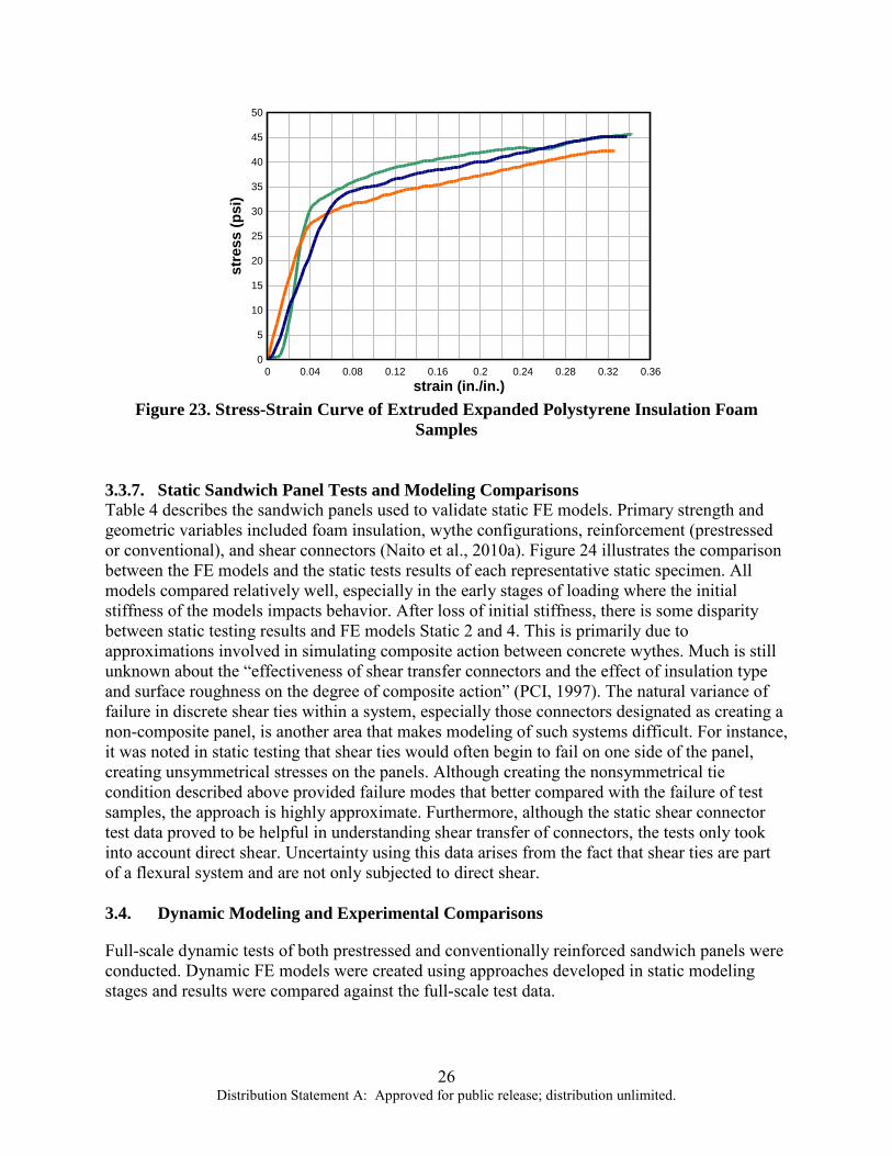
In static compressive testing of foam materials, strain was recorded as engineering strain. It is evident in Figures 21–23 that if the sandwich panel system allows the foam to become compressed, theoretically, a large amount of energy will be absorbed due to the large strains of the foam. However, the observed sandwich panel system response does not support the notion that foam is a major source of energy dissipation. The significant axial rigidity of the shear ties results in the transfer of force from the exterior to interior concrete wythe, and thereby precluding large strains developing in the foam before the ultimate strength of the panel is reached. Furthermore, the initial elastic portion of the foam materials in compression is on the order of 15 to 20 psi, whereas the ultimate static pressure capacity of the panels used in the static and dynamic testing is less than 5 psi. Therefore, even without considering the axial resistance provided by the ties, the foam insulation would strain only a small percentage of its ultimate strain ability at the ultimate load capacity of the panel.
strain (in./in.)
stre
ss (p
si)
0 0.04 0.08 0.12 0.16 0.2 0.24 0.28 0.32 0.360
2
4
6
8
10
12
14
16
18
Figure 21. Stress-Strain Curve of Expanded Polystyrene Insulation Foam Samples
strain (in./in.)
stre
ss (p
si)
0 0.04 0.08 0.12 0.16 0.2 0.24 0.28 0.32 0.360
5
10
15
20
25
30
35
40
Figure 22. Stress-Strain Curve of Polyisocyanruate Insulation Foam Samples
26 Distribution Statement A: Approved for public release; distribution unlimited.
strain (in./in.)
stre
ss (p
si)
0 0.04 0.08 0.12 0.16 0.2 0.24 0.28 0.32 0.360
5
10
15
20
25
30
35
40
45
50
Figure 23. Stress-Strain Curve of Extruded Expanded Polystyrene Insulation Foam
Samples 3.3.7. Static Sandwich Panel Tests and Modeling Comparisons Table 4 describes the sandwich panels used to validate static FE models. Primary strength and geometric variables included foam insulation, wythe configurations, reinforcement (prestressed or conventional), and shear connectors (Naito et al., 2010a). Figure 24 illustrates the comparison between the FE models and the static tests results of each representative static specimen. All models compared relatively well, especially in the early stages of loading where the initial stiffness of the models impacts behavior. After loss of initial stiffness, there is some disparity between static testing results and FE models Static 2 and 4. This is primarily due to approximations involved in simulating composite action between concrete wythes. Much is still unknown about the “effectiveness of shear transfer connectors and the effect of insulation type and surface roughness on the degree of composite action” (PCI, 1997). The natural variance of failure in discrete shear ties within a system, especially those connectors designated as creating a non-composite panel, is another area that makes modeling of such systems difficult. For instance, it was noted in static testing that shear ties would often begin to fail on one side of the panel, creating unsymmetrical stresses on the panels. Although creating the nonsymmetrical tie condition described above provided failure modes that better compared with the failure of test samples, the approach is highly approximate. Furthermore, although the static shear connector test data proved to be helpful in understanding shear transfer of connectors, the tests only took into account direct shear. Uncertainty using this data arises from the fact that shear ties are part of a flexural system and are not only subjected to direct shear. 3.4. Dynamic Modeling and Experimental Comparisons
Full-scale dynamic tests of both prestressed and conventionally reinforced sandwich panels were conducted. Dynamic FE models were created using approaches developed in static modeling stages and results were compared against the full-scale test data.

27 Distribution Statement A: Approved for public release; distribution unlimited.
Table 4. Static Sandwich Panel Validation Matrix
Specimen Reinforcement Type
Wythe Conf. Insulation Panel Reinforcement
(Longitudinal/Transverse) Shear Ties
Static 1 conventionally reinforced 323 XPS # 3 /#3 fiberglass
composite
Static 2 conventionally reinforced 623 XPS # 3 / WWR fiberglass
non-composite
Static 3 prestressed 333 XPS 3/8 strand / # 3 fiberglass composite
Static 4 prestressed 333 XPS 3/8 strand / # 3 steel c-clip non-composite
Static 5 prestressed 323 EPS 3/8 strand / WWR carbon-fiber composite
Static 6 prestressed 323 EPS 3/8 strand / WWR steel c-clip non-composite

28 Distribution Statement A: Approved for public release; distribution unlimited.
displacement (in.)
displacement (cm)
pres
sure
(psi
)
pres
sure
(kPa
)
Static 1
0
0
1
2.54
2
5.08
3
7.62
4
10.16
5
12.7
6
15.24
7
17.78
8
20.32
0 0
1 6.89
2 13.78
3 20.67
4 27.56
5 34.45
6 41.34Static AverageFEM
displacement (in.)
displacement (cm)
pres
sure
(psi
)
pres
sure
(kPa
)
Static 2
0
0
1
2.54
2
5.08
3
7.62
4
10.16
5
12.7
6
15.24
7
17.78
8
20.32
0 0
1 6.89
2 13.78
3 20.67
4 27.56
5 34.45
6 41.34Static AverageFEM
displacement (in.)
displacement (cm)
pres
sure
(psi
)
pres
sure
(kPa
)
Static 3
0
0
1
2.54
2
5.08
3
7.62
4
10.16
5
12.7
6
15.24
7
17.78
8
20.32
0 0
1 6.89
2 13.78
3 20.67
4 27.56
5 34.45
6 41.34Static AverageFEM
displacement (in.)
displacement (cm)
pres
sure
(psi
)
pres
sure
(kPa
)
Static 4
0
0
1
2.54
2
5.08
3
7.62
4
10.16
5
12.7
6
15.24
7
17.78
8
20.32
0 0
1 6.89
2 13.78
3 20.67
4 27.56
5 34.45
6 41.34Static AverageFEM
displacement (in.)
displacement (cm)
pres
sure
(psi
)
pres
sure
(kPa
)
Static 5
0
0
1
2.54
2
5.08
3
7.62
4
10.16
5
12.7
6
15.24
7
17.78
8
20.32
0 0
1 6.89
2 13.78
3 20.67
4 27.56
5 34.45
6 41.34Static AverageFEM
displacement (in.)
displacement (cm)
pres
sure
(psi
)
pres
sure
(kPa
)
Static 6
0
0
1
2.54
2
5.08
3
7.62
4
10.16
5
12.7
6
15.24
7
17.78
8
20.32
0 0
1 6.89
2 13.78
3 20.67
4 27.56
5 34.45
6 41.34Static AverageFEM
Figure 24. Static Test Results vs Finite Element Model Comparisons
3.4.1. Full-scale Dynamic Tests Full-scale dynamic experiments were broken into two parts: Dynamic Series I (Naito et al., 2009a) and Dynamic Series II (Naito et al., 2010b). All experiments were conducted by the Airbase Technologies Division of AFRL at Tyndall Air Force Base, Florida. The Dynamic Series I test data was not used in the finite element comparisons presented in this section; however, Dynamic Series I data was used for comparison purposes for SDOF prediction methodology discussed in Section 5. For each Dynamic Series II experiment, eight sandwich panels (four single span panels and four multi-span panels) were subjected to a small pre-detonation load followed by a large primary detonation. An overall view of the test arena used

29 Distribution Statement A: Approved for public release; distribution unlimited.
for full-scale dynamic tests is shown in Figure 25. The purpose of the pre-detonation load was to excite the elastic natural frequencies of the panels so that the frequencies could be compared to those of respective FE models. The primary detonation loading was designed to deform the panels well beyond their elastic limit and, if possible, close to their ultimate strength. Dynamic tests consisted of both single span and multi-span precast sandwich panels, with either prestressed or conventional reinforcement. All panels were designed to be thermally efficient by using either glass fiber or carbon fiber reinforced shear connectors (Naito et al. 2010b). Foam insulation consisted of either EPS or XPS. Midspan deflections and reflected pressures were recorded. Reflected pressures on the single span reaction structure were recorded in three locations along the midspan. Multi-span reaction structure reflected pressure gauges were located longitudinally and transversely in three locations for a total of nine locations of pressure recordings. Dynamic deflections were also recorded at the middle of each span, which were used as the predominant comparison between testing and FE data.
Figure 25. Test Setup for Full Scale Dynamic Tests with Single Span Reaction Structure
(left) and Multi-span Reaction Structure (right) (Naito et all., 2010b) Table 5 provides an overview of the panel designs used in the full-scale dynamic experiments. Single span specimens were tested in the single span reaction structure; therefore specimens are referenced by an “SS” followed by the specimen identification number. Multi-span panels were tested in the multi-span reaction structure; therefore multi-span panels are referenced with an “MS” followed by the specimen identification number. For each detonation, a representative reflected pressure was created by averaging the recorded pressures to obtain a pressure curve with both a comparable peak pressure and peak impulse. The four different load regimes involved in the tests (which provide a basic understanding of the time domain involved) are non-dimensionally represented in Figure 26 and Table 6 using the lowest peak pressure and impulse as the basis.
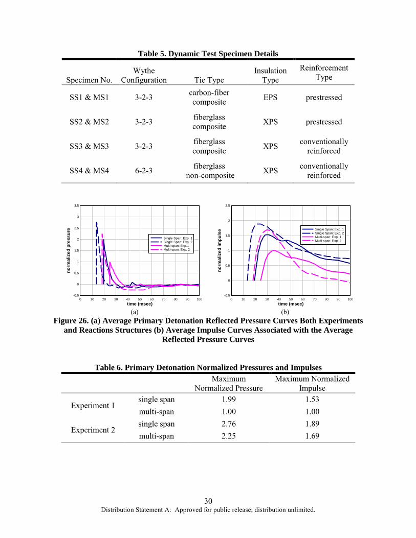
30 Distribution Statement A: Approved for public release; distribution unlimited.
Table 5. Dynamic Test Specimen Details
Specimen No. Wythe
Configuration Tie Type Insulation
Type Reinforcement
Type
SS1 & MS1 3-2-3 carbon-fiber composite EPS prestressed
SS2 & MS2 3-2-3 fiberglass composite XPS prestressed
SS3 & MS3 3-2-3 fiberglass composite XPS conventionally
reinforced
SS4 & MS4 6-2-3 fiberglass non-composite XPS conventionally
reinforced
time (msec)
norm
aliz
ed p
ress
ure
0 10 20 30 40 50 60 70 80 90 100-0.5
0
0.5
1
1.5
2
2.5
3
3.5
Single Span: Exp. 1Single Span: Exp. 2Multi-span: Exp.1Multi-span: Exp. 2
(a)
time (msec)
norm
aliz
ed im
puls
e
0 10 20 30 40 50 60 70 80 90 100-0.5
0
0.5
1
1.5
2
2.5
Single Span: Exp. 1Single Span: Exp. 2Multi-span: Exp. 1Multi-span: Exp. 2
(b)
Figure 26. (a) Average Primary Detonation Reflected Pressure Curves Both Experiments and Reactions Structures (b) Average Impulse Curves Associated with the Average
Reflected Pressure Curves
Table 6. Primary Detonation Normalized Pressures and Impulses Maximum
Normalized Pressure Maximum Normalized
Impulse
Experiment 1 single span 1.99 1.53 multi-span 1.00 1.00
Experiment 2 single span 2.76 1.89 multi-span 2.25 1.69

31 Distribution Statement A: Approved for public release; distribution unlimited.
3.4.2. Dynamic Finite Element Models All dynamic models were created using the statically validated parameters and methods, including material models, the concrete damage plasticity model, and the multipoint constraint approach for the modeling of shear connectors. Models were developed and analyzed using LS-DYNA, an advanced general purpose finite element code capable of solving complex nonlinear mechanics problems (LSTC, 2009). The “MAT_CONCRETE_DAMAGE_R3” concrete model was used for concrete elements. The “MAT_072R3” concrete element was used in LS-DYNA for concrete elements. Steel elements were modeled using the “MAT_PLASTIC_KINEMATIC” material model. Steel elements were modeled using the “MAT_003” element in LS-DYNA. Rigid elements were used for boundary conditions. Transient pressures were applied uniformly across the exterior surface of the panel. Overall, the modeling approach was designed to focus on the flexural response of the sandwich panel system, and care was taken so that the models would not become unstable due to local punching at the supports, although punching failure was noted in some of the multi-span tests. 3.4.3. Simulation of Prestressing Effects in LS-DYNA LS-DYNA provides several methods for including initial conditions prior to a transient load application. For simulating prestressing in concrete structures, the “CONTROL_DYNAMIC_RELAXATION” feature provides a procedure for combining the initial static loading with a subsequent dynamic load case. The dynamic relaxation method was used in this study to initialize the stress in the panel systems due to the prestressing strand elements, and then the dynamic load case was run based on this initial condition. Definition of the initial stress in truss elements was made by setting ELFORM=3, and assigning values to RAMPT (ramp time for stress initialization by dynamic relaxation), and STRESS (initial stress in truss elements) in the keyword card “SECTION_BEAM”. The initial stress was initialized by setting IDRFLG=-1 in the “CONTROL_DYNAMIC_RELAXATION” card. Then, after stress initialization, the load case was applied dynamically by setting IMFLAG=0 in the “CONTROL_IMPLICIT_GENERAL” card. 3.4.4. Simulation of Dynamic Increase Factors The sudden nature of blast loading and the acceleration of structural mass result in high rates of strain. At these higher strain rates, the strength of both concrete and steel can increase. The ratio of the dynamic to static strength is referred to as the dynamic increase factor (DIF) and is commonly reported as a function of strain rate. Simulation of steel reinforcement typically uses the Cowper and Symonds model (Eq. 18), which scales the yield stress depending upon the strain rate (Stouffer and Dame, 1996).
1/
1P
DIFCε = +
(18)
In the Cowper Symonds model, ε represents strain rate. Also, C and P are parameters that depend upon the steel properties. Mild steel was considered in this study; therefore, C and P were 40 and 5, respectively (Stouffer and Dame, 1996). A curve relating the dynamic increase factor of concrete vs. strain-rate provided within LS-DYNA was used as the basis for strain-rate effects. However, the flexural response proved very sensitive to the strain rate effects definition. The input data associated with the range of strain

32 Distribution Statement A: Approved for public release; distribution unlimited.
rates observed from the modeling output was magnified up to five times the LS-DYNA default to reflect the upper limits of previously published research (Malvar and Crawford, 1998; Malvar and Ross, 1998). Figure 27 demonstrates the default DIF curve used by LS-DYNA.
strain-rate (1/s)
DIF
-5 -4 -3 -2 -1 0 1 2 3 4 51
1.25
1.5
1.75
2
2.25
2.5
compression tension
Figure 27. LS-DYNA Default Curve for Concrete DIF
3.4.5. Dynamic Sandwich Panel Experiment and FE Model Comparisons Full-scale dynamic test results for Dynamic Series II were compared with the results of FE models subjected to similar loading. Loading curves were developed by analyzing recorded reflected pressures and creating a representative curve that would be similar in both peak positive and negative pressure as well as impulse. Single span dynamic models were completed first, followed by multi-span dynamic models. For comparison purposes, only pre-detonation loading from Experiment 1 was evaluated due to the similarities of pressure for both experiments. Both single span and multi-span models were compared against two primary detonation pressures. 3.4.6. Single Span Results and Comparisons All single span models exhibited very similar initial response, and maximum midspan displacement was consistently within reasonable error. The reasons for these error differences include: challenges with accurately replicating the support conditions (the FE model boundary conditions were not created to simulate the local failures observed in the dynamic tests), variability of the foam insulation, shear tie variability and ambiguities (i.e. response of shear ties in a high strain-rate environment), and DIF ambiguity. Single span primary detonation comparisons are displayed in Figure 28 and Figure 29 for Experiments 1 and Experiment 2, respectively.

33 Distribution Statement A: Approved for public release; distribution unlimited.
time (msec)
disp
lace
men
t (in
.)
0 10 20 30 40 50 60 70 80 90 100 110 120 130 140 150-3
-2
-1
0
1
2
3
4
5
6ExperimentFE Model
(a)
time (msec)
disp
lace
men
t (in
.)
0 10 20 30 40 50 60 70 80 90 100 110 120 130 140 150-3
-2
-1
0
1
2
3
4
5
6ExperimentFE Model
(b)
time (msec)
disp
lace
men
t (in
)
0 10 20 30 40 50 60 70 80 90 100 110 120 130 140 150-3
-2
-1
0
1
2
3
4
5
6ExperimentFE Model
(c)
time (msec)di
spla
cem
ent (
in.)
0 10 20 30 40 50 60 70 80 90 100 110 120 130 140 150-3
-2
-1
0
1
2
3
4
5
6ExperimentFE Model
(d)
Figure 28. Experiment 1–Primary Detonation Measured Midspan Displacement vs. Finite Element Displacement Comparison for (a) SS1, (b) SS2, (c), SS3, (d) SS4
time (msec)
disp
lace
men
t (in
.)
0 10 20 30 40 50 60 70 80 90 100 110 120 130 140 150-3
-2
-1
0
1
2
3
4
5
6
7
8ExperimentFE Model
(a)
time (msec)
disp
lace
men
t (in
.)
0 10 20 30 40 50 60 70 80 90 100 110 120 130 140 150-3
-2
-1
0
1
2
3
4
5
6
7
8ExperimentFE model
(b)
time (msec)
disp
lace
men
t (in
.)
0 10 20 30 40 50 60 70 80 90 100 110 120 130 140 150-3
-2
-1
0
1
2
3
4
5
6
7
8ExperimentFE Model
(c)
time (msec)
disp
lace
men
t (in
.)
0 10 20 30 40 50 60 70 80 90 100 110 120 130 140 150-3
-2
-1
0
1
2
3
4
5
6
7
8ExperimentFE model
(d)
Figure 29. Experiment 2–Primary Detonation Measured Midspan Displacement vs. Finite Element Midspan Displacement Comparison for (a) SS1, (b) SS2, (c) SS3, (d) SS4

34 Distribution Statement A: Approved for public release; distribution unlimited.
As mentioned above, only Experiment 1 pre-detonation loading (Fig. 30) was considered for frequency comparison of test specimens to FE models. Pre-detonation results (Table 7, Fig. 31) were reasonably accurate for the first half sine wave of displacement. After the first half period, variance between the FE models and experimental damping are quite apparent. This is most likely due to the absence of damping characteristics, such as real-world boundary conditions causing friction. Models were considered acceptable if the first half sine wave of displacement correlated well.
Table 7. Pre-detonation Comparison of Single Span Experimental and FE Model Natural
Period
Panel Experimental First Half Sine Wave,
msec
FE Model First Half Sine Wave, msec Error
SS1 30.0 34.5 15.0 % SS2 20.0 23.7 18.5 % SS3 25.1 24.5 2.4 % SS4 23.2 21.2 8.6 %
time (msec)
pres
sure
(psi
)
impu
lse
(psi
-impu
lse)
0 10 20 30 40 50 60 70 80 90 100 110 120-3 -12
-2 -8
-1 -4
0 0
1 4
2 8
3 12
4 16
5 20
6 24
7 28
8 32PressureImpulse
Figure 30. Pre-detonation Pressure and Impulse for Single Span Reaction Structure–
Experiment 1

35 Distribution Statement A: Approved for public release; distribution unlimited.
time (msec)
disp
lace
men
t (in
.)
0 50 100 150 200 250 300 350 400 450 500-0.4
-0.3
-0.2
-0.1
0
0.1
0.2
0.3
0.4ExperimentFE Model
(a)
time (msec)
disp
lace
men
t (in
.)
p
0 50 100 150 200 250 300 350 400 450 500-0.4
-0.3
-0.2
-0.1
0
0.1
0.2
0.3
0.4ExperimentFE Model
(b)
time (msec)
disp
lace
men
t (in
.)
0 50 100 150 200 250 300 350 400 450 500-0.4
-0.3
-0.2
-0.1
0
0.1
0.2
0.3
0.4ExperimentFE Model
(c)
time (msec)
disp
lace
men
t (in
.)
0 50 100 150 200 250 300 350 400 450 500-0.4
-0.3
-0.2
-0.1
0
0.1
0.2
0.3
0.4ExperimentFE Model
(d)
Figure 31. Experiment 1–Pre-detonation Measured Midspan Displacement vs. Finite Element Midspan Displacement Comparison for (a) SS1, (b) SS2, (c) SS3, (d) SS4
3.4.7. Multi-span Results and Comparisons The multi-span panels generally exhibited good correlation between FE models and experimental results, especially in regards to initial response. Multi-span primary detonation comparisons for Experiment 1 are displayed in Figures 32 and 33; Multi-span primary detonation comparisons for Experiment 2 are displayed in Figures 34 and 35. All variability issues involving single span validation are also true for multi-span validation. The modeling methodology did not simulate the relatively flexible boundary conditions of the multi-span test panels, and therefore the multi-span FE results did not include the local failures observed with the experimental panels; this is especially significant for panels tested in Experiment 2 due to its much larger reflected pressure. Local failures were most prevalent for second floor frame connections due to the large tributary area of the connections. For instance, the response of panel MS4 was influenced by the failure of its second floor connection (Fig. 36).

36 Distribution Statement A: Approved for public release; distribution unlimited.
time (msec)
disp
lace
men
t (in
.)
0 10 20 30 40 50 60 70 80 90 100 110 120 130 140 150-2
-1
0
1
2
3
4ExperimentFE Model
(a)
time (msec)
disp
lace
men
t (in
.)
0 10 20 30 40 50 60 70 80 90 100 110 120 130 140 150-2
-1
0
1
2
3
4ExperimentFE Model
(b)
time (msec)
disp
lace
men
t (in
.)
0 10 20 30 40 50 60 70 80 90 100 110 120 130 140 150-2
-1
0
1
2
3
4
5
6ExperimentFE Model
(c)
time (msec)di
spla
cem
ent (
in.)
0 10 20 30 40 50 60 70 80 90 100 110 120 130 140 150-2
-1
0
1
2
3
4ExperimentFE Model
(d)
Figure 32. Experiment 1–Primary Detonation Measured First Floor Midspan Displacement vs. Finite Element Midspan Displacement Comparison for (a) MS1, (b) MS2, (c) MS3,
(d) MS4
time (msec)
disp
lace
men
t (in
.)
0 10 20 30 40 50 60 70 80 90 100 110 120 130 140 150-2
-1
0
1
2
3
4ExperimentFE model
(a)
time (msec)
disp
lace
men
t (in
.)
0 10 20 30 40 50 60 70 80 90 100 110 120 130 140 150-2
-1
0
1
2
3
4ExperimentFE Model
(b)
time (msec)
disp
lace
men
t (in
.)
0 10 20 30 40 50 60 70 80 90 100 110 120 130 140 150-2
-1
0
1
2
3
4ExperimentFE Model
(c)
time(msec)
disp
lace
men
t (in
)
0 10 20 30 40 50 60 70 80 90 100 110 120 130 140 150-2
-1
0
1
2
3
4ExperimentFE Model
(d)
Figure 33. Experiment 1– Primary Detonation Measured Second Floor Midspan Displacement vs. Finite Element Midspan Displacement Comparison for (a) MS1, (b) MS2,
(c) MS3, (d) MS4

37 Distribution Statement A: Approved for public release; distribution unlimited.
time (msec)
disi
plac
emen
t (in
.)
0 20 40 60 80 100 120 140 160 180 200-3
-2
-1
0
1
2
3
4
5
6
7
8
9ExperimentFE Model
(a)
time (msec)
disp
lace
men
t (in
.)
0 20 40 60 80 100 120 140 160 180 200-3
-2
-1
0
1
2
3
4
5
6
7
8
9ExperimentFE Model
(b)
time (msec)
disp
lace
men
t (in
.)
0 20 40 60 80 100 120 140 160 180 200-3
-2
-1
0
1
2
3
4
5
6
7
8
9ExperimentFE Model
(c)
time (msec)di
spla
cem
ent (
in.)
0 20 40 60 80 100 120 140 160 180 200-3
-2
-1
0
1
2
3
4
5
6
7
8
9ExperimentFE Model
(d)
Figure 34. Experiment 2– Primary Detonation Measured First Floor Midspan Displacement vs. Finite Element Midspan Displacement Comparison for (a) MS1, (b) MS2,
(c) MS3, (d) MS4
time (msec)
disp
lace
men
t (in
.)
0 10 20 30 40 50 60 70 80 90 100 110 120 130 140 150-3
-2
-1
0
1
2
3
4
5
6ExperimentFE Model
(a)
time (msec)
disp
lace
men
t (in
.)
0 10 20 30 40 50 60 70 80 90 100 110 120 130 140 150-3
-2
-1
0
1
2
3
4
5
6ExperimentFE Model
(b)
time (msec)
disp
lace
men
t (in
.)
0 10 20 30 40 50 60 70 80 90 100 110 120 130 140 150-3
-2
-1
0
1
2
3
4
5
6ExperimentFE Model
(c)
Figure 35. Primary Detonation Measured Second Floor Midspan Displacement vs. Finite Element Midspan Displacement Comparison for (a) MS2, (b) MS3, (c) MS4

38 Distribution Statement A: Approved for public release; distribution unlimited.
Figure 36. Localized Effects Along the Second Floor Support
The FE prediction of the multi-span pre-detonation pressure response (Fig. 37) was reasonably accurate for the first quarter sine wave of displacement. Multi-span pre-detonation responses are displayed in Figures 38 and 39. Due to differences between the FE modeling approach and true multi-span connections, pre-detonation results for multi-span panels experienced more variance than the simple spans. A second floor frame (Fig. 40) was fabricated and intended to react similar to a second floor system would react under similar loading conditions. All multi-span panels were connected to this frame; therefore, approximately after the first quarter-sine wave of midspan displacement, an interaction between the panels and the flexible floor system was apparent. The FE models used linear spring elements to approximate the resistance of the second floor frame (Fig. 40), leading to the discrepancy between experimental and FE model pre-detonation response.
time (msec)
pres
sure
(psi
)
impu
sle
(psi
-mse
c)
0 10 20 30 40 50 60 70 80 90 100 110 120-2 -8
-1 -4
0 0
1 4
2 8
3 12
4 16
5 20
6 24
7 28
8 32PressureImpulse
Figure 37. Pre-detonation Pressure and Impulse for Multi-span Reactions Structure–
Experiment 1

39 Distribution Statement A: Approved for public release; distribution unlimited.
time (msec)
disp
lace
men
t (in
.)
0 100 200 300 400 500-0.4
-0.3
-0.2
-0.1
0
0.1
0.2
0.3
0.4ExperimentFE Model
(a)
time (msec)
disp
lace
men
t (in
.)
0 100 200 300 400 500-0.4
-0.3
-0.2
-0.1
0
0.1
0.2
0.3
0.4ExperimentFE Model
(b)
time (msec)
disp
lace
men
t (in
.)
0 100 200 300 400 500-0.5
-0.4
-0.3
-0.2
-0.1
0
0.1
0.2
0.3
0.4
0.5ExperimentFE Model
(c)
time (msec)di
spla
cem
ent (
in.)
0 100 200 300 400 500-0.4
-0.3
-0.2
-0.1
0
0.1
0.2
0.3
0.4ExperimentFE Model
(d)
Figure 38. Experiment 1– Pre-detonation Measured First Floor Midspan Displacement vs. Finite Element Midspan Displacement Comparison for (a) MS1, (b) MS2, (c) MS3, (d) MS4
time (msec)
disp
lace
men
t (in
.)
0 100 200 300 400 500-0.4
-0.3
-0.2
-0.1
0
0.1
0.2
0.3
0.4ExperimentFE Model
(a)
time (msec)
disp
lace
men
t (in
.)
0 100 200 300 400 500-0.4
-0.3
-0.2
-0.1
0
0.1
0.2
0.3
0.4ExperimentFE Model
(b)
time (msec)
disp
lace
men
t (in
.)
0 100 200 300 400 500-0.4
-0.3
-0.2
-0.1
0
0.1
0.2
0.3
0.4ExperimentFE Model
(c)
time (msec)
disp
lace
men
t (in
.)
0 100 200 300 400 500-0.4
-0.3
-0.2
-0.1
0
0.1
0.2
0.3
0.4ExperimentFE Model
(d)
Figure 39. Pre-detonation Measured Second Floor Midspan Displacement vs. Finite Element Midspan Displacement Comparison for (a) MS1, (b) MS2, (c) MS3, (d) MS4

40 Distribution Statement A: Approved for public release; distribution unlimited.
Table 8. Pre-detonation Comparison of Multi-span Experimental and FE Model Natural Period
Panel
Experimental First Quarter Sine Duration,
msec
FE Model First Quarter Sine Duration, msec Error
MS1 ~20.0 ~17.5 ~14 % MS2 ~19.1 ~23.5 ~23 % MS3 ~19.5 ~24.0 ~23% MS4 ~13.3 ~15.0 ~13%
Figure 40. Second Floor Support Frame Allowing Interaction Between the Behaviors of All
Multi-span Panels Attached

41 Distribution Statement A: Approved for public release; distribution unlimited.
4. STUDY OF BLAST RESPONSE BEHAVIOR OF SANDWICH PANELS
4.1. Introduction
Due to the high costs of full-scale dynamic testing, finite element simulation can serve as a crucial tool in evaluating the behavior of structural systems and components subjected to blast loads. After validating the FE models with experimental data, the models were used to evaluate the failure mechanisms of sandwich panels subjected to impulse loads. The study consisted of energy plots, progression of reinforcement strain vs. time, and reaction forces. Energy plots display the “flow” of energy through time and help determine the importance of mass and the strain of reinforcement in sandwich panels. The reinforcement strain vs. time plots describe the development of hinges throughout time and their locations. Also, dynamic reaction forces were extracted from FE models and compared to experimental data. 4.2. Energy Dissipation
Energy provided by an impulse load on a sandwich panel can be dissipated in two ways: internal and external energy. Energy involving straining and/or failure of concrete wythes, steel reinforcement, foam insulation, or shear connectors is internal energy. External energy involves the kinetic energy of the mass of the sandwich panel that is accelerated by the impulse load. Energy plots can provide insight into the role each component takes in absorbing and dissipating energy. The two components that are assured to impact energy absorption are the mass of the concrete wythes and the yielding of steel reinforcement. There is a vast amount of data studying the insulation capabilities of the foam; however, the absorption of energy by the insulating foam in a high-strain environment is unknown. Also unknown is the role of shear connectors in transferring energy between the concrete wythes. FE models indicated that, early within the response of panels, shear connectors absorbed energy axially through the nonlinear spring of the MPC approach that represented the axial strength of the tie. This would signify brief displacement of the shear connector which would give the external concrete wythe the opportunity to provide more energy across the entire surface of the foam. Kinetic energy plots display the significant role the mass of concrete plays in dissipating the energy of the system (Fig. 41). It is important to notice the similarities between panels SS2 and SS3. Figure 41b displays the kinetic energy of a prestressed sandwich panel with a 3-2-3 wythe configuration; Figure 41c has the same 3-2-3 configuration but is conventionally reinforced. However, both models used an MPC approach that simulated a composite fiberglass shear connector. The kinetic energy plots of both panels have similar maximum kinetic energy for both concrete wythes and behavior continues to appear similar throughout response. This reinforces the fact that the shear connector resistance and effects on composite action are crucial components of the overall behavior of the sandwich panel when subjected to blast loads. As expected, the six-inch interior concrete wythe of panel SS4 displays relatively large kinetic energy in comparison to the thee-inch exterior wythe due to the increased mass (Fig. 41d).

42 Distribution Statement A: Approved for public release; distribution unlimited.
time (msec)
ener
gy (l
b-in
)
0 20 40 60 80 100 120 140 160 180 2000
10000
20000
30000
40000
50000
60000
70000
80000
90000interior concrete wytheexterior concrete wythereinforcementfoam insulation
(a)
time (msec)
ener
gy (l
b-in
)
0 20 40 60 80 100 120 140 160 180 2000
10000
20000
30000
40000
50000
60000
70000interior concrete wytheexterior concrete wythereinforcementfoam insulation
(b)
time (msec)
ener
gy (l
b-in
)
0 20 40 60 80 100 120 140 160 180 2000
10000
20000
30000
40000
50000
60000
70000interior concrete wytheexterior concrete wythereinforcementfoam insulation
(c) time (msec)
ener
gy (l
b-in
)
0 20 40 60 80 100 120 140 160 180 2000
10000
20000
30000
40000
50000
60000interior concrete wytheexterior concrete wythereinforcementfoam insulation
(d)
Figure 41. Kinetic Energy of Sandwich Panel System Components–Experiment 1; (a) SS1, (b) SS2, (c) SS3, (d) SS4
4.3. Strain Distribution
Strain of reinforcement was plotted across the height of one prestressed specimen and both conventionally reinforced models simulated Experiment 1, the single span test specimens. The strain was plotted every five milliseconds beginning at zero until the maximum strain of the reinforcement was reached. As can be seen in Figures 42-44, the strain for all specimens reaches maximum at a point in time beyond the positive phase of the impulse load (Fig.45). This is because the inertial resistance of the sandwich panel specimens results in a relatively slow flexural response. The yielding of reinforcement at midspan causes a hinge, which helps to dissipate energy.

43 Distribution Statement A: Approved for public release; distribution unlimited.
height (in.)
stra
in (i
n./in
.)
0 12 24 36 48 60 72 84 96 108 120 132 144-0.005
0
0.005
0.01
0.015
0.020 msec5 msec10 msec15 msec20 msec25 msec
Figure 42. SS1–Experiment 1: Strain of Reinforcement of Interior Concrete Wythe Across
Panel Height Over Time
height (in.)
stra
in (i
n./in
.)
0 12 24 36 48 60 72 84 96 108 120 132 144-0.005
0
0.005
0.01
0.015
0.02
0.025
0.03
0.035
0.040 msec5 msec10 msec15 msec20 msec25 msec30 msec35 msec
Figure 43. SS3–Experiment 1: Strain of Reinforcement of Interior Concrete Wythe Across
Panel Height Over Time

44 Distribution Statement A: Approved for public release; distribution unlimited.
height (in.)
stra
in (i
n./in
.)
0 12 24 36 48 60 72 84 96 108 120 132 144-0.005
0
0.005
0.01
0.015
0.02
0.025
0.03
0.035
0.040 msec5 msec10 msec15 msec20 msec25 msec30 msec35 msec40 msec
Figure 44. SS4–Experiment 1: Strain of Reinforcement of Interior Concrete Wythe Across
Panel Height Over Time
time (msec)
norm
aliz
ed p
ress
ure
0 10 20 30 40 50 60 70 80 90 100 110 120-0.5
0
0.5
1
1.5
2
2.5
3Experiment 1
Figure 45. Average Pressure for Experiment 1 Used for Finite Element Models Simulating
Single Span Test Specimens

45 Distribution Statement A: Approved for public release; distribution unlimited.
4.4. Reaction Force vs. FE Models
For the Dynamic Series II experiments, reaction forces were measured at the top of all single span specimens using two load cells (Fig. 46). FE models were prepared with rigid boundaries mirroring the load cell locations of the experimental panels. Overall reaction force was recorded on the rigid boundaries throughout time. FE models showed higher reactions than those recorded in full-scale dynamic experiments. Comparisons of measured reaction force and FE models were done for Experiment 1 of Dynamic Series II (Figs. 47–50). For panel SS4, one load cell was not operational during the experiment; in order to make a comparison, the recorded reaction from the one load cell that was operational is compared against its representative rigid boundary in the model in Figure 50. Although comparisons initially correlate well, it is possible binding of the two load cell system impeded the load cells from recording the load history in its entirety. Concrete structural components are typically designed to withstand both inbound flexural response and outward rebound of the component. This design criterion usually means reinforcing is symmetric, since stresses reverse on the rebound response of the component. Connections used for precast components subjected to blast are normally designed with small to zero dynamic increase factors. Ductility of the flexural resistance of the component is just as important to the connection as the ductility of the connection itself. If the component is too rigid, more force will be transmitted to reactions, possibility causing connection failure.
Figure 46. Load Cells Recording Reaction Force for Single Span Specimens

46 Distribution Statement A: Approved for public release; distribution unlimited.
time (msec)
reac
tion
forc
e (lb
s)
0 5 10 15 20 25 30 35 40 45 50-25000
0
25000
50000
75000
100000
125000
150000
175000
200000
225000SS1-MeasuredFE Model
Figure 47. Comparison of Measured Total Reaction Force and Recorded FE Model
Reaction Forces for Experiment 1–SS1
time (msec)
reac
tion
forc
e (lb
s)
0 5 10 15 20 25 30 35 40 45 50-25000
0
25000
50000
75000
100000
125000
150000
175000
200000SS2-MeasuredFE Model
Figure 48. Comparison of Measured Total Reaction Force and Recorded FE Model
Reaction Forces for Experiment 1–SS2

47 Distribution Statement A: Approved for public release; distribution unlimited.
time (msec)
reac
tion
forc
e (lb
s)
0 5 10 15 20 25 30 35 40 45 50-50000
-25000
0
25000
50000
75000
100000
125000
150000
175000
200000SS3-MeasuredFE Model
Figure 49. Comparison of Measured Total Reaction Force and Recorded FE Model
Reaction Forces for Experiment 1–SS3
time (msec)
reac
tion
forc
e (lb
s)
0 5 10 15 20 25 30 35 40 45 50-10000
0
10000
20000
30000
40000
50000
60000
70000
80000SS4-MeasuredFE Model
Figure 50. Comparison of Measured Total Reaction Force and Recorded FE Model
Reaction Forces for Experiment 1–SS4

48 Distribution Statement A: Approved for public release; distribution unlimited.
5. SINGLE-DEGREE-OF-FREEDOM (SDOF) MODEL DEVELOPMENT
5.1. Introduction
One common approach for designing structural systems and components for impulse loads is to use a SDOF system that will represent the maximum displacement response of the structure. The central-difference approach is a relatively simple numerical method that can be used to integrate the equation of motion at discrete time intervals. This section focuses on the development of SDOF models for predicting the blast response of precast sandwich panels and comparisons to current design tools. The finite element models presented in the prior sections were used to expand comparison data for developing the SDOF methodology. The development of resistance definitions used in the SDOF models was based on Army Corps of Engineers design methodology (DoD 2008). Two sandwich panel resistance definitions were produced: a composite resistance based upon perfect composite action between the concrete wythes and a non-composite resistance based upon zero composite action. From analysis of these boundaries, a weighted resistance was calculated by weighting composite and non-composite responses with percentages that represent approximate composite action of the actual systems. 5.2. General SDOF Methodology
Structural systems can be broken down into infinite degrees of freedom. However, it is useful to simplify the motion of an object to a single-degree-of-freedom. Structural components subjected to blast are commonly designed with the midspan displacement as the single-degree-of-freedom. SDOF methodology is based upon the equation of motion of an object subjected to a force that causes an acceleration of the mass of the object (Eq. 19). ( )mx cx kx F t+ + = (19) The force ( )F t is resisted by the mass of the object ( m ), damping constant ( c ), and spring/stiffness constant ( k ), multiplied by the acceleration ( x ), velocity ( x ), and displacement ( x ), respectively. A system with the corresponding equation of motion is represented with a free-body diagram as shown in Figure 51. An equivalent SDOF equation of motion can be developed from the characteristics of the structural component (Fig. 51). An arbitrary beam with length l and shape function y(y) with arbitrary mass per unit length m that resists the arbitrarily distributed load v(y) represents the structural system which must be effectively described as a single-degree-of-freedom. The SDOF equation of motion must be transformed from characteristics of the continuous component to equivalent characteristics of the SDOF system. Therefore, the characteristics of mass ( m ), damping constant ( c ), and spring/stiffness constant ( k ) and dynamic load (F) are multiplied by constants such that
eM
mKm
= (20)
eD
cKc
= (21)
eS
kKk
= (22)

49 Distribution Statement A: Approved for public release; distribution unlimited.
eL
FKF
= (23)
where F and m are the total force (F=vl) and total mass (m= m l) of the system, where l is the length of the structural component . The constants KS and KD can be replaced with the constant KL. This is done because KS and KL can be shown to be equal to each other (Biggs, 1964) and although mathematically it is not correct to replace KD with KL, is does not affect the outcome of the systems peak dynamic response since damping has negligible effect on the peak response. The equation of motion can then be written as: ( )M L L LK mx K cx K kx K F t+ + = (24) A structure with continuous mass and distributed force will have both equivalent mass and equivalent force as follows:
2 ( )l
eM m y dyψ= ∫ (25)
( ) ( )l
eF v y y dyψ= ∫ (26)
where, ( )yψ is the equivalent assumed-shape function of the system. By dividing the equation of motion of Equation 24 with LK , the equation of motion can now be written as the following:
( )M
L
K mx cx kx F tK
+ + = (27)
where MLM
L
K KK
= is the load-mass factor. Biggs (1964) presents several load-mass factors for
beams and slabs having various types of support conditions.
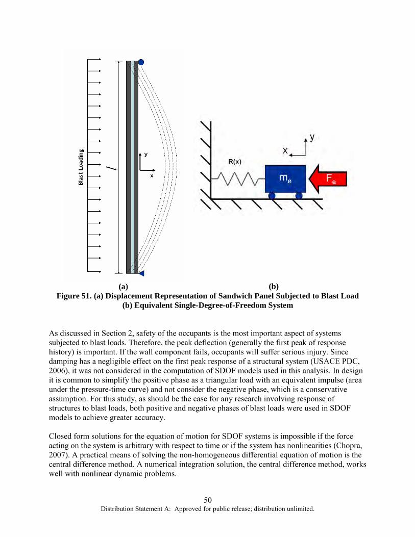
50 Distribution Statement A: Approved for public release; distribution unlimited.
(a)
(b) Figure 51. (a) Displacement Representation of Sandwich Panel Subjected to Blast Load
(b) Equivalent Single-Degree-of-Freedom System As discussed in Section 2, safety of the occupants is the most important aspect of systems subjected to blast loads. Therefore, the peak deflection (generally the first peak of response history) is important. If the wall component fails, occupants will suffer serious injury. Since damping has a negligible effect on the first peak response of a structural system (USACE PDC, 2006), it was not considered in the computation of SDOF models used in this analysis. In design it is common to simplify the positive phase as a triangular load with an equivalent impulse (area under the pressure-time curve) and not consider the negative phase, which is a conservative assumption. For this study, as should be the case for any research involving response of structures to blast loads, both positive and negative phases of blast loads were used in SDOF models to achieve greater accuracy. Closed form solutions for the equation of motion for SDOF systems is impossible if the force acting on the system is arbitrary with respect to time or if the system has nonlinearities (Chopra, 2007). A practical means of solving the non-homogeneous differential equation of motion is the central difference method. A numerical integration solution, the central difference method, works well with nonlinear dynamic problems.

51 Distribution Statement A: Approved for public release; distribution unlimited.
The central difference method is based upon a finite difference approximation of the velocity and acceleration of the structure. If the time step, t∆ , is chosen correctly, the time derivatives of displacement (i.e. velocity and acceleration) can be approximated as:
1 1
2i i
ix xx
t+ −−
=∆
(28)
1 12
2( )
i i ii
x x xxt
+ −− +=
∆ (29)
Substituting these values for acceleration and velocity into Equation 19 gives
1 1 1 12
2( ) 2
i i i i ii i
x x x x xm c kx Ft t
+ − + −− + −+ + =
∆ ∆ (30)
Disregarding the damping term due to its negligible contribution to first peak response and solving for 1ix + gives
21 1( ) 2i i
i i iF kxx t x xm m+ −
= − ∆ + −
(31)
It should be noted that by placing initial conditions within Equation 29 and continuing to disregard damping, it can be found that
i iF kx xm m
− =
(32)
The SDOF model uses Equation 31 to solve for response but with a few modifications. First, the mass is the effective mass of the system, LMK m . The initial location at 1it − is input as 0, and the
displacement after the first time step ( it ) is input as half (1/2) the 2 2( ) ( )i iF t kx t
m m∆ ∆
− term of
Equation 31 as is suggested in Biggs (1964). This ensures that all terms are present after the second time step to calculate response. The pressure is called from the input load curve according to the appropriate time, it , then divided by the effective mass factor. The effective mass, em , is calculated by finding the unit mass of the wall and then dividing by the appropriate transformation factor (either elastic or plastic). The resistance is initially input as zero and called from the input resistance curve according to the appropriate previous steps displacement, then divided by the effective mass. Within the prediction model, the effective mass is manually changed from the elastic effective mass to the plastic effective mass at the point where resistance is no longer elastic. The acceleration, x , is calculated as Equation 32, with the exception that
ikx is the appropriate resistance as discussed previously. The term 2( )x t∆ is needed to calculate the appropriate displacement, x , for each time step. Figure 52 displays how this is applied within a spreadsheet format.
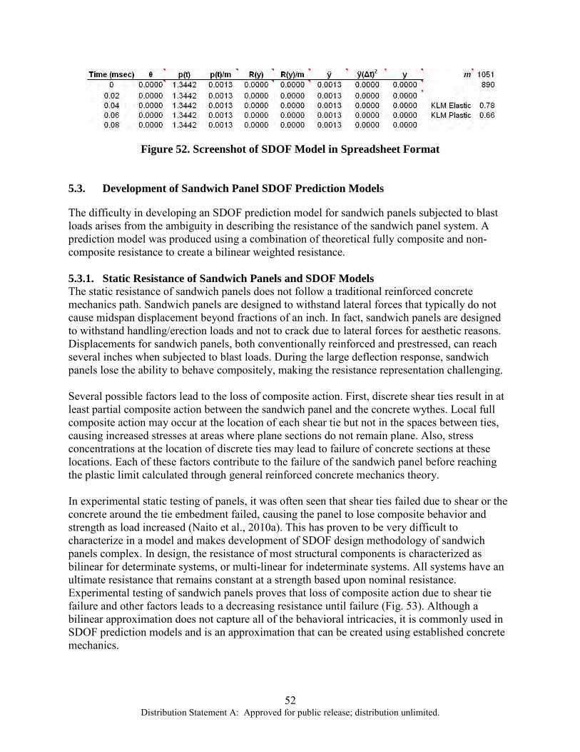
52 Distribution Statement A: Approved for public release; distribution unlimited.
Figure 52. Screenshot of SDOF Model in Spreadsheet Format 5.3. Development of Sandwich Panel SDOF Prediction Models
The difficulty in developing an SDOF prediction model for sandwich panels subjected to blast loads arises from the ambiguity in describing the resistance of the sandwich panel system. A prediction model was produced using a combination of theoretical fully composite and non-composite resistance to create a bilinear weighted resistance. 5.3.1. Static Resistance of Sandwich Panels and SDOF Models The static resistance of sandwich panels does not follow a traditional reinforced concrete mechanics path. Sandwich panels are designed to withstand lateral forces that typically do not cause midspan displacement beyond fractions of an inch. In fact, sandwich panels are designed to withstand handling/erection loads and not to crack due to lateral forces for aesthetic reasons. Displacements for sandwich panels, both conventionally reinforced and prestressed, can reach several inches when subjected to blast loads. During the large deflection response, sandwich panels lose the ability to behave compositely, making the resistance representation challenging. Several possible factors lead to the loss of composite action. First, discrete shear ties result in at least partial composite action between the sandwich panel and the concrete wythes. Local full composite action may occur at the location of each shear tie but not in the spaces between ties, causing increased stresses at areas where plane sections do not remain plane. Also, stress concentrations at the location of discrete ties may lead to failure of concrete sections at these locations. Each of these factors contribute to the failure of the sandwich panel before reaching the plastic limit calculated through general reinforced concrete mechanics theory. In experimental static testing of panels, it was often seen that shear ties failed due to shear or the concrete around the tie embedment failed, causing the panel to lose composite behavior and strength as load increased (Naito et al., 2010a). This has proven to be very difficult to characterize in a model and makes development of SDOF design methodology of sandwich panels complex. In design, the resistance of most structural components is characterized as bilinear for determinate systems, or multi-linear for indeterminate systems. All systems have an ultimate resistance that remains constant at a strength based upon nominal resistance. Experimental testing of sandwich panels proves that loss of composite action due to shear tie failure and other factors leads to a decreasing resistance until failure (Fig. 53). Although a bilinear approximation does not capture all of the behavioral intricacies, it is commonly used in SDOF prediction models and is an approximation that can be created using established concrete mechanics.

53 Distribution Statement A: Approved for public release; distribution unlimited.
displacement (in.)
pres
sure
(psi
)
0 0.5 1 1.5 2 2.5 3 3.5 4 4.5 5 5.5 6 6.5 70
1
2
3
4
5
6
7
8Experimental ResistanceBi-linear Resistance
Figure 53. Comparison of Experimental Resistance to Bilinear Resistance Curve
5.3.2. Correlation with Current Prediction Methods The Protective Design Center (PDC) of the Army Corps of Engineers developed an analysis tool entitled SBEDS (Single-Degree-of-Freedom Blast Effects Design Spreadsheet) which creates SDOF models for predicting the response for a wide range of common structural components. The mechanics and structural dynamics of the systems were based upon the technical manual titled “Structures to Resist the Effects of Accidental Explosions” (formally referred to as TM5-1300, it has been entered into the Unified Facilities Criteria as UFC 3-340-02). 5.3.3. Resistance Calculation The PDC has published a document entitled “User’s Guide for the Single-Degree-of-Freedom Blast Effects Design Spreadsheet (SBEDS)” describing the methods incorporated from UFC 3-340-02 in the development of predictive SDOF models for structural components (USACE PDC, 2006). SDOF models were developed using this document for the prediction of sandwich panel designs used in full-scale experiments. The sandwich panel SDOF model resistances were created by calculating a 100% composite resistance and a 0% composite resistance, and creating a weighted average resistance, represented as a bilinear resistance for experimental samples. Figure 54 displays screenshots of the spreadsheet implementing the bilinear resistance methodology for generation of a prediction SDOF. This bilinear resistance was then used to determine a response of the dynamic samples subjected to the two experimental blast loads.

54 Distribution Statement A: Approved for public release; distribution unlimited.
Figure 54. Screenshots of Developed SDOF Prediction Analysis Spreadsheet Resistance
Input 5.3.4. Material Dynamic Properties Calculation As previously discussed, both concrete and reinforcing steel strengths are sensitive to the rate of loading. It is known that, as strain rate increases, the concrete compressive strength also increases; there is some debate upon the factor that should be used. Often the DIF is chosen to be

55 Distribution Statement A: Approved for public release; distribution unlimited.
1.19 for design purposes, and this factor was used in all SDOF models for this analysis. The equation for calculating dynamic concrete strength is ' ' ( )dc c e af f K K DIF= (33) where 'dcf is the concrete dynamic compression strength, 'cf is the concrete minimum specified compression strength, aK is the concrete aging factor, and eK is the static strength increase factor, and the DIF is described above. The factor aK accounts for the observed increase in concrete compressive strength over time and is conservatively taken as 1.1 in most cases. The factor eK accounts for the observation that most material strengths exceed specified minimums and is conservatively taken as 1.1 unless in-field material testing leads one to use another value. Like concrete strength, reinforcing steel dynamic strength uses a static strength increase factor and a DIF. ( )dy y ef f K DIF= (34) Factors used depend upon the reinforcement type as seen in Table 9 (USACE PDC, 2006). Most prestressed sandwich panels use seven-wire strand of either Grade 250 or Grade 270; it is customary to give prestressing strand DIF and eK values of 1.0.
Table 9. Dynamic Yield Strength for Conventional Reinforcement (USACE PDC, 2006) Type of Steel Yield Strength
(psi) Ultimate Strength
(psi) Ke DIF
ASTM A615, A616, A706
(Grade 60) 60,000 90,000 1.1 1.17
ASTM A615 (Grade 40)
40,000 75,000 1.1 1.17
ASTM, A496 (Welded Wire Fabric)
70,000 80,000 1.0 1.1
The ultimate dynamic moment capacity of a conventionally reinforced concrete beam or slab is represented by Equation 35, where sA is the area of steel, d is the depth of tension reinforcement, and b is the width of concrete compression block. Singly reinforced cross-sections (described as Type I cross-sections in PDC 6-02) are often assumed for all cross-sections as a conservative approach. The ultimate dynamic moment capacity for reinforced concrete slabs and beams described in Equation 35 is utilized by SBEDS without any consideration of a Type II cross section (Type II cross-sections are doubly reinforced and also assumes concrete cannot carry compression due to crushing).
'1.7s dy
du s dydc
A fM A f d
bf
= −
(35)
The ultimate dynamic moment capacity of prestressed concrete beams and slabs is represented by Equation 36, where psA is the area of prestressed reinforcement, a (Eq. 37) is the depth of the equivalent rectangle compression stress block, pd is the distance from the extreme compression

56 Distribution Statement A: Approved for public release; distribution unlimited.
fiber to the centroid of the prestressed reinforcement and psf (Eq. 38) is the average stress in the prestressed reinforcement at ultimate load.
2 2u ps ps p s dya aM A f d A f d = − + −
(36)
( )
'0.85ps ps s dy
dc
A f A fa
f b+
= (37)
( )' '1
1 'p pu dyps pu p
dc p dc
f dff f
f d fγ
ρ ρ ρβ
= − + −
(38)
where fpu is the ultimate tensile strength of the prestressed reinforcement, γp is a factor that depends upon the type of prestressing reinforcement used, and β1 is a factor relating the depth of the equivalent rectangular compressive stress block to the neutral axis depth. The factors ρp, ρ, and ρ’ represent the prestressed reinforcement ratio, the reinforcing ratio for non-prestressed tension reinforcement, and the reinforcing ratio of non-prestressed compression reinforcement, respectively. For conventionally reinforced sandwich panels, the moment of inertia used to calculate displacements, which in turn are used in resistance curves, is an average (Equation 7) of gross moment of inertia, Ig, of the entire cross section and a cracked moment of inertia, Ic (Equation 8).
( )
2g c
a
I II
+= (39)
3cI Fd= (40)
Equation 40 is an approximation of the cracked moment of inertia and uses the factor F chosen from the charts taken from UFC 340-02 (Figure 55). The modular ratio used in conjunction with the cracked moment of inertia factor charts is stated as the following:
s
c
EnE
= (41)
where n is the modular ratio, Es the modulus of elasticity for steel, and Ec is the modulus of elasticity for concrete. The modulus of elasticity for concrete is equal to: 1.5 '33c c cE w f= (42) where cw is the unit weight of concrete – normally 145 lbs/ft3. The moment of inertia, Ic, of prestressed beams or slabs is also an average of gross and cracked moment of inertia as defined in Equation 39 for nonprestressed beams or slabs. The cracked moment of inertia for prestressed beams or slabs is as follows:
2 1/21 ( )c ps pI nA d ρ = − (43)

57 Distribution Statement A: Approved for public release; distribution unlimited.
Figure 55. Coefficients of Cracked Moment of Inertia (UFC 2-340-02)
5.4. SDOF Prediction Model Comparisons
SDOF prediction models using the aforementioned bilinear weighted resistance were compared against full-scale dynamic tests and FE models. 5.4.1. SDOF Prediction Model Matrix Full-scale dynamic tests were completed in two series. The first series of tests were completed in 2006 and included tests of two precast/prestressed sandwich panels subjected to various blast pressures and compared to standard conventionally reinforced concrete panels used as controls (Naito et al. 2009b). Test specimens were 30 feet tall with support conditions approximated as simple supports. In total, Dynamic Series I consisted of five separate detonations. Prediction models were used to predict responses for panels subjected Detonations 2 and 3. Dynamic Series II consisted of two experiments each consisting of a pre-detonation loading and a primary loading as discussed in Section 3. Only single span specimens subjected to primary detonations were used for SDOF predictions. All single span Dynamic Series II specimens had a clear span of 9.7 feet and simple supports assumed (Naito et al., 2010b). In order to increase the data that could be used to assess the SDOF prediction models, FE modeling was used to test span lengths not involved in the dynamic full-scale tests. Also, fixed-fixed boundary conditions were modeled to compare prediction models ability in simulating such conditions. In total, 22 SDOF prediction models were compared against either full-scale measured displacements or FE models. Table 10 shows all prediction models and their comparative basis.

58 Distribution Statement A: Approved for public release; distribution unlimited.
Table 10. SDOF Prediction Model Comparison Matrix Dynamic Series I
Specimen Clear Span (ft)
Wythe Configuration Tie Type Boundary
Conditions Reinforcement
Type Detonation 2 30 3-2-3 Solid concrete zones simple prestressed
Detonation 3 30 3-2-3 carbon fiber composite simple prestressed
Dynamic Series II -Experiment 1 & 2
Specimen No. Clear Span
Wythe Configuration Tie Type Boundary
Conditions Reinforcement
Type
SS1 9.7 3-2-3 carbon fiber composite simple prestressed
SS2 9.7 3-2-3 fiberglass composite simple prestressed
SS3 9.7 3-2-3 fiberglass composite simple conventional
SS4 9.7 6-2-3 fiberglass non-composite simple conventional
FE Modeling Data Expansion Set
Specimen No. Clear Span
Wythe Configuration Tie Type Boundary
Conditions Reinforcement
Type
FE-1 18.7 3-2-3 carbon fiber composite simple prestressed
FE-2 18.7 3-2-3 fiberglass composite simple prestressed
FE-3 18.7 3-2-3 fiberglass composite simple conventional
FE-4 18.7 6-2-3 fiberglass non-composite simple conventional
FE-5 18.7 3-2-3 carbon fiber composite fixed-fixed prestressed
FE-6 18.7 3-2-3 fiberglass composite fixed-fixed prestressed
FE-7 18.7 3-2-3 fiberglass composite fixed-fixed conventional
FE-8 18.7 6-2-3 fiberglass non-composite fixed-fixed conventional
FE-9 9.7 3-2-3 carbon fiber composite fixed-fixed prestressed
FE-10 9.7 3-2-3 fiberglass composite fixed-fixed prestressed
FE-11 9.7 3-2-3 fiberglass composite fixed-fixed conventional
FE-12 9.7 6-2-3 fiberglass non-composite fixed-fixed conventional
5.4.2. SDOF Prediction Model Comparisons – Dynamic Series I The first precast/prestressed specimen tested in Dynamic Series I used solid concrete sections as connectors between the interior and exterior concrete wythes. Panels using solid concrete

59 Distribution Statement A: Approved for public release; distribution unlimited.
sections for shear transfer are considered to give the panel composite behavior only during service loads. Therefore, based upon this design parameter and to fit the Dynamic Series I data set, the SDOF prediction model used a weighted average with 65% composite, 35% non-composite resistance. These percentages were continuously used throughout all predictions for prestressed sandwich panels using composite connectors. The solid-zone panel was subjected to two detonations in the Dynamic Series I tests of varying pressures, the first being low loading and causing minimal damage. The second detonation was larger and considered a more viable data set for comparison of SDOF prediction models developed. As seen in Figure 56, the SDOF prediction is accurate against the measured response. It should be noted that, since this panel had been subjected to a prior detonation, there is a possibility that the measured displacement may be higher than would be expected without previous testing. Figure 56 compares the SDOF responses with a composite resistance, a non-composite resistance, the weighted resistance, and the measured solid-zone panel response from Dynamic Series I, Detonation 2.
time (msec)
supp
ort r
otat
ion
(deg
rees
)
0 10 20 30 40 50 60 70 80 90 100 1100.00
0.25
0.50
0.75
1.00
1.25
Composite SDOFNon-composite SDOFRecommended Weighted Resistance SDOFSolid zone panel - Detonation 2 - Measured
Figure 56. Dynamic Series I, Detonation 2 Measured Displacement Comparison to SDOF
Prediction Using Weighted Resistance The second precast/prestressed panel tested in Dynamic Series I was subjected to Detonations 3, 4, and 5. The panel used a composite carbon fiber shear connector intended to provide composite action to panels subjected to their designed service loads; therefore, the prestressed/composite weighted resistance of 65% composite resistance, 35% non-composite resistance was used. The prediction was lower than the measured response, which in general is not a good qualifier when creating a prediction method for structural systems subjected to blasts. As seen in Figure 57, the prediction was accurate, within a reasonable margin of error. Table 11 demonstrates the percent difference between weighted resistance predictions and measured data for the Dynamic Series I tests. No other detonations were considered for the carbon-fiber-reinforced-polymer (CFRP) panel due to the large permanent displacement seen after each detonation. The panels tested in Dynamic Series I represent the largest clear spans (30 feet) tested in a full-scale dynamic experiment. Sandwich panels become more efficient to build, transport, and erect as span length increases.

60 Distribution Statement A: Approved for public release; distribution unlimited.
Although the full-scale dynamic data set for sandwich panels of this height is small, their importance is significant due to the common use of large span lengths in practice.
time (msec)
supp
ort r
otat
ion
(deg
rees
)
0 20 40 60 80 100 120 140 160 180 2000.00
0.25
0.50
0.75
1.00
1.25
1.50
1.75
2.00
Composite SDOFNon-composite SDOFRecommended Weighted Resistance SDOFCFRP panel - Detonation 3 -Measured
Figure 57. Dynamic Series I, Detonation 3 Measured Displacement Comparison to SDOF
Prediction Using Weighted Resistance
Table 11. Percent Difference, Dynamic Series I SDOF Prediction vs. Measured Support Rotation
Panel Predicted Support Rotation, degrees
Measured Support Rotation, degrees % Difference
Solid-Zone Panel 0.886 0.884 0.2% CRFP Panel 1.365 1.432 4.7 %
5.4.3. SDOF Prediction Model Comparisons – Dynamic Series II Next, SDOF predictions using weighted resistances were compared for all single span specimens tested in Dynamic Series II. Dynamic Series II consisted of two experiments. SDOF predictions using weighted resistances were created for primary detonations for both experiments. All composite panels used a weighted resistance of 65% composite resistance and 35% non-composite resistance. Predictions for the only non-composite panel in Dynamic Series II used a weighted resistance of 30% composite resistance, 70% non-composite resistance. As can be seen in Figures 58 and 59 and in Tables 12 and 13, all weighted resistance predictions accurately predicted response within an acceptable margin of error.

61 Distribution Statement A: Approved for public release; distribution unlimited.
time (msec)
supp
ort r
otat
ion
(deg
rees
)
0 10 20 30 40 50 60 70 800
1
2
3
4
5
6
7
Composite SDOFNon-composite SDOFRecommended Weighted Resistance SDOFSS1-Measured
(a)
time (msec)
supp
ort r
otat
ion
(deg
rees
)
0 10 20 30 40 50 60 70 800
1
2
3
4
5
6
7
Composite SDOFNon-composite SDOFRecommended Weighted Resistance SDOFSS2-Measured
(b)
time (msec)
supp
ort r
otat
ion
(deg
rees
)
0 10 20 30 40 50 60 70 800
1
2
3
4
5
6
7
Composite SDOFNon-composite SDOFRecommended Weighted Resistance SDOFSS3-Measured
(c)
time (msec)
supp
ort r
otat
ion
(deg
rees
)
0 10 20 30 40 50 60 70 800
1
2
3
4
5
6
7
Composite SDOFNon-composite SDOFRecommended Weighted Resistance SDOFSS4-Measured
(d)
Figure 58. Evaluation of Weighted Resistance Prediction Method vs. Measured Data: Dynamic Series II–Experiment 1 (a) SS1 (b) SS2 (c) SS3 (d) SS4
Table 12. Percent Difference, Dynamic Series II–Experiment 1 SDOF Prediction vs. Measured Support Rotation
Panel Predicted Support Rotation, degrees
Measured Support Rotation, degrees % Difference
SS1 3.77 3.39 11.2 SS2 3.96 2.92 35.6 SS3 4.98 4.78 4.2 SS4 3.64 3.42 6.4

62 Distribution Statement A: Approved for public release; distribution unlimited.
time (msec)
supp
ort r
otat
ion
(deg
rees
)
0 10 20 30 40 50 60 70 80 90 1000
1
2
3
4
5
6
7
8
9
10
Composite SDOFNon-composite SDOFRecommended Weighted Resistance SDOFSS1-Measured
(a)
time (msec)
supp
ort r
otat
ion
(deg
rees
)
0 10 20 30 40 50 60 70 80 90 1000
1
2
3
4
5
6
7
8
9
10
Composite SDOFNon-composite SDOFRecommended Weighted Resistance SDOFSS2-Measured
(b)
time (msec)
supp
ort r
otat
ion
(deg
rees
)
0 10 20 30 40 50 60 70 80 90 1000
1
2
3
4
5
6
7
8
9
10
Composite SDOFNon-composite SDOFRecommended Weighted Resistance SDOFSS3-Measured
(c)
time (msec)
supp
ort r
otat
ion
(deg
rees
)
0 10 20 30 40 50 60 70 80 90 1000
1
2
3
4
5
6
7
8
9
10
Composite SDOFNon-Composite SDOFRecommended Weighted Resistance SDOFSS4-Measured
(d)
Figure 59. Evaluation of Weighted Resistance Prediction Method vs. Measured Data: Dynamic Series II–Experiment 2 (a) SS1 (b) SS2 (c) SS3 (d) SS4
Table 13. Percent Difference, Dynamic Series II–Experiment 2 SDOF Prediction vs. Measured Support Rotation
Panel Predicted Support Rotation, degrees
Measured Support Rotation, degrees % Difference
SS1 5.72 5.86 -2.4 SS2 5.95 5.63 5.7 SS3 7.17 6.87 4.4 SS4 5.22 4.45 17.3
5.4.4. Resistance and Energy Comparisons SDOF predictions were created for each specimen using recorded experimental resistance in order to study the viability of using a bilinear weighted resistance curve to replace actual resistance in the SDOF system. After support rotation comparison, an SDOF model was created using the experimental resistance of each panel. The predicted response from the weighted resistance SDOF was compared against the response from the experimental resistance SDOF. As
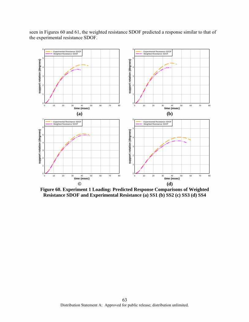
63 Distribution Statement A: Approved for public release; distribution unlimited.
seen in Figures 60 and 61, the weighted resistance SDOF predicted a response similar to that of the experimental resistance SDOF.
time (msec)
supp
ort r
otat
ion
(deg
rees
)
0 10 20 30 40 50 60 70 800
1
2
3
4
5
6Experimental Resistance SDOFWeighted Resistance SDOF
(a)
time (msec)
supp
ort r
otat
ion
(deg
rees
)
0 10 20 30 40 50 60 70 800
1
2
3
4
5
6Experimental Resistance SDOFWeighted Resistance SDOF
(b)
time (msec)
supp
ort r
otat
ion
(deg
rees
)
0 10 20 30 40 50 60 70 800
1
2
3
4
5
6
7Experimental Resistance SDOFWeighted Resistance SDOF
©
time (msec)
supp
ort r
otat
ion
(deg
rees
)
0 10 20 30 40 50 60 70 800
1
2
3
4
5
6Experimental Resistance SDOFWeighted Resistance SDOF
(d)
Figure 60. Experiment 1 Loading: Predicted Response Comparisons of Weighted Resistance SDOF and Experimental Resistance (a) SS1 (b) SS2 (c) SS3 (d) SS4

64 Distribution Statement A: Approved for public release; distribution unlimited.
time (msec)
supp
ort r
otat
ion
(deg
rees
)
0 10 20 30 40 50 60 70 800
1
2
3
4
5
6
7
8
9Experimental Resistance SDOFWeighted Resistance SDOF
(a)
time (msec)
supp
ort r
otat
ion
(deg
rees
)
0 10 20 30 40 50 60 70 800
1
2
3
4
5
6
7
8
9Experimental Resistance SDOFWeighted Resistance SDOF
(b)
time (msec)
supp
ort r
otat
ion
(deg
rees
)
0 10 20 30 40 50 60 70 800
1
2
3
4
5
6
7
8
9Experimental Resistance SDOFWeighted Resistance SDOF
(c)
time (msec)
supp
ort r
otat
ion
(deg
rees
)
0 10 20 30 40 50 60 70 800
1
2
3
4
5
6
7
8
9Experimental Resistance SDOFWeighted Resistance SDOF
(d)
Figure 61. Experiment 2 Loading: Predicted Response Comparisons of Weighted Resistance SDOF and Experimental Resistance (a) SS1 (b) SS2 (c) SS3 (d) SS4
Next, the weighted and experimental resistances were directly compared for all specimens using loadings from both experiments. Both weighted and experimental resistances were recorded until the maximum SDOF predicted displacement response was reached. Figures 62-65 show the resistance and energy comparisons for Experiment 1 loading. Figures 66-69 show the resistance and energy comparisons for Experiment 2 loading. Also, the area under the resistance curves were integrated, giving the total amount of energy absorbed through resistance. This serves as a good comparative basis since the bilinear resistance can be conservative or un-conservative depending upon the displacement of the system as seen in Figure 70. In this case, a resistance is considered conservative when it would lead to a larger displacement in the SDOF model. If the bilinear weighted resistance is lower than the experimental resistance at the same displacement it is conservative. It should be noted that Figure 70 is only an example and that bilinear weighted resistance for other designs does not always follow the path of being unconservative initially and becoming more conservative as displacement increases. In Figure 72 for example, the bilinear resistance begins slightly conservative, then becomes unconservative, returns to conservative, and then becomes highly unconservative as displacement increases. The bilinear weighted resistance was chosen as a means of creating a global representation of energy absorbed by the system, not for its accuracy in determining resistance at any one displacement. The only

65 Distribution Statement A: Approved for public release; distribution unlimited.
specimen examined using the weighted resistance SDOF prediction methods that exhibited high amount of variability was panel SS4, the non-composite conventionally reinforced panel. Non-composite panels, as seen in testing, have high rates of variability due to the differing degrees of a non-composite action.
displacement (in.)
tota
l loa
d (lb
)
ener
gy (l
b-in
)
0 1 2 3 4 4.50 0
5000 25000
10000 50000
15000 75000
20000 100000
Weighted ResistanceExperimental ResistanceWeighted Resistance EnergyExperimental Energy
Figure 62. Experiment 1 Loading: Resistance and Energy for SS1
displacement (in.)
tota
l loa
d (lb
)
ener
gy (l
b-in
.)
0 1 2 3 4 50 0
5000 20000
10000 40000
15000 60000
20000 80000
Weighted ResistanceExperimental ResistanceWeighted Resistance EnergyExperimental Energy
Figure 63. Experiment 1 Loading: Resistance and Energy for SS2

66 Distribution Statement A: Approved for public release; distribution unlimited.
displacement (in.)
tota
l loa
d (lb
)
ener
gy (l
b-in
.)
0 1 2 3 4 5 60 0
2000 8000
4000 16000
6000 24000
8000 32000
10000 40000
Weighted ResistanceExperimental EnergyWeighted Resistance EnergyExperimental Energy
Figure 64. Experiment 1 Loading: Resistance and Energy for SS3
displacement (in.)
tota
l loa
d (lb
)
ener
gy (l
b-in
.)
0 1 2 3 4 4.50 0
1000 4000
2000 8000
3000 12000
4000 16000
5000 20000
6000 24000
Weighted ResistanceExperimental ResistanceWeighted Resistance EnergyExperimental Energy
Figure 65. Experiment 1 Loading: Resistance and Energy for SS4

67 Distribution Statement A: Approved for public release; distribution unlimited.
displacement (in.)
tota
l loa
d (lb
)
ener
gy (l
b-in
.)
0 1 2 3 4 5 6 7 7.50 0
5000 30000
10000 60000
15000 90000
20000 120000
Weighted ResistanceExperimental ResistanceWeight Resistance EnergyExperimental Energy
Figure 66. Experiment 2 Loading: Resistance and Energy for SS1
displacement (in.)
tota
l loa
d (lb
)
ener
gy (l
b-in
.)
0 1 2 3 4 5 6 70 0
2500 15000
5000 30000
7500 45000
10000 60000
12500 75000
15000 90000
17500 105000
20000 120000
Weighted ResistanceExperimental ResistanceWeighted Resistance EnergyExperimental Energy
Figure 67. Experiment 2 Loading: Resistance and Energy for SS2

68 Distribution Statement A: Approved for public release; distribution unlimited.
displacement (in.)
tota
l loa
d (lb
)
ener
gy (l
b-in
.)
0 1 2 3 4 5 6 70 0
2000 10000
4000 20000
6000 30000
8000 40000
10000 50000
Weighted ResistanceExperimental EnergyWeighted Resistance EnergyExperimental Energy
Figure 68. Experiment 2 Loading: Resistance and Energy for SS3
displacement (in.)
tota
l loa
d (lb
)
ener
gy (l
b-in
.)
0 1 2 3 4 5 60 0
1000 5000
2000 10000
3000 15000
4000 20000
5000 25000
6000 30000
Weighted ResistanceExperimental ResistanceWeight Resistance EnergyExperimental Energy
Figure 69. Experiment 2 Loading: Resistance and Energy for SS4

69 Distribution Statement A: Approved for public release; distribution unlimited.
displacement (in.)
tota
l loa
d (lb
)
ener
gy (l
b-in
.)
0 1 2 3 4 5 60 0
1000 5000
2000 10000
3000 15000
4000 20000
5000 25000
6000 30000
7000 35000
bilinear weighted resistance begins to provides conservative predicted response
bilinear weighted resistance provides unconservative predicted reponse
Weighted ResistanceExperimental Resistance
Figure 70. Demonstration of Bilinear Resistance Impact on Conservative Response
Prediction 5.4.5. SDOF Prediction Model Comparisons – FE Modeling Finite element modeling is a less expensive means of studying structural components subjected to blast loads compared to full-scale testing. In order to increase the amount of data available for weighted resistance SDOF prediction comparisons, FE models with boundary conditions and span lengths that varied from full-scale dynamic tests were created. The FE models were created with the same reinforcement schedules and shear connector properties. Weighted resistance SDOF comparisons were previously completed for sandwich panels with span lengths of 9.7 ft and 30 ft. An intermediate span length of 18.7 ft was studied using FE models. Also, models using fixed-fixed connections were created and compared against weighted resistance SDOF responses. Every finite element model created for the purpose of comparison to SDOF prediction had a response greater than that of the SDOF prediction. Some of this variability between FE models and predictions can be explained. Much greater variability was seen between FE models and predictions with fixed boundary conditions due to the inability to accurately model fixed boundary conditions. FE models were created with an artificial fixed-fixed boundary condition formed from two objects at each end that restricted the boundaries; this is somewhat inaccurate since the weighted resistance SDOF prediction methodology considers fixed boundary condition to be more similar to continuous beams or columns. Figure 71 and Table 14 present the comparisons between FE model responses and weight resistance SDOF prediction for 18 ft clear span, simply-supported sandwich panels. Figure 72 and Table 15 present the comparisons between FE model responses and weight resistance SDOF prediction for 18 ft clear span sandwich panels with fixed-fixed boundary conditions. Figure 73 and Table 16 present the

70 Distribution Statement A: Approved for public release; distribution unlimited.
comparisons between FE model responses and weighted resistance SDOF prediction for 9.7 ft clear span sandwich panels with fixed-fixed boundary conditions.
time (msec)
supp
ort r
otat
ion
(deg
rees
)
0 10 20 30 40 50 60 70 80 90 1000
1
2
3
4
5
6
Composite SDOFNon-composite SDOFRecommended Weighted Resistance SDOFFE Model
(a)
time (msec)
supp
ort r
otat
ion
(deg
rees
)
0 10 20 30 40 50 60 70 80 90 1000
1
2
3
4
5
6
Composite SDOFNon-composite SDOFRecommended Weighted Resistance SDOFFE Model
(b)
time (msec)
supp
ort r
otat
ion
(deg
rees
)
0 10 20 30 40 50 60 70 80 90 1000
1
2
3
4
5
6
Composite SDOFNon-composite SDOFRecommended Weighted Resistance SDOFFE Model
(c)
time (msec)
supp
ort r
otat
ion
(deg
rees
)
0 10 20 30 40 50 60 70 80 90 1000
1
2
3
4
Composite SDOFNon-composite SDOFRecommended Weighted Resistance SDOFFE Model
(d)
Figure 71. FE Model Response vs. SDOF Prediction Using Weighted Resistance for (a) FE-1, (b) FE-2, (c) FE-3, (d) FE-4
Table 14. Percent Difference, SDOF Prediction vs. FE Model Response
Panel Predicted Support Rotation, degrees
FE Model Support Rotation, degrees % Difference
FE-1 3.92 4.99 -21.4 FE-2 3.91 5.05 -22.6 FE-3 4.49 5.08 -11.6 FE-4 3.06 3.16 -3.2

71 Distribution Statement A: Approved for public release; distribution unlimited.
time (msec)
supp
ort r
otat
ion
(deg
rees
)
0 10 20 30 40 50 60 70 80 90 1000
1
2
3
4
5
Composite SDOfNon-composite SDOFRecommended Weighted Resistance SDOFFE Model
(a)
time (msec)
supp
ort r
otat
ion
(deg
rees
)
0 10 20 30 40 50 60 70 80 90 1000
1
2
3
4
5
Composite SDOFNon-composite SDOFRecommended Weighted Resistance SDOFFE Model
(b)
time (msec)
supp
ort r
otat
ion
(deg
rees
)
0 10 20 30 40 50 60 70 80 90 1000
1
2
3
4
5
Composite SDOFNon-composite SDOFRecommended Weighted Resistance SDOFFE Model
(c)
time (msec)
supp
ort r
otat
ion
(deg
rees
)
0 10 20 30 40 50 60 70 80 90 1000
1
2
3
4
5
Composite SDOFNon-composite SDOFRecommended Weighted Resistance SDOFFE Model
(d)
Figure 72. FE Model Response vs. SDOF Prediction Using Weighted Resistance for (a) FE-5, (b) FE-6, (c) FE-7, (d) FE-8
Table 15. Percent Difference, SDOF Prediction vs. FE Model Response
Panel Predicted Support Rotation, degrees
FE Model Support Rotation, degrees % Difference
FE-5 2.94 4.30 -31.7 FE-6 3.02 4.03 -25.1 FE-7 3.71 4.03 -7.9 FE-8 2.55 3.77 -32.4

72 Distribution Statement A: Approved for public release; distribution unlimited.
time (msec)
supp
ort r
otat
ion
(deg
rees
)
0 10 20 30 40 50 600
1
2
3
4
Composite SDOFNon-composite SDOFRecommended Weighted Resistance SDOFFE Model
(a)
time (msec)
supp
ort r
otat
ion
(deg
rees
)
0 10 20 30 40 50 600
1
2
3
4
5
Composite SDOFNon-composite SDOFRecommended Weighted Resistance SDOFFE Model
(b)
time (msec)
supp
ort r
otat
ion
(deg
rees
)
0 10 20 30 40 50 60 700
1
2
3
4
5
6
7
8
Composite SDOFNon-composite SDOFRecommended Weighted Resistance SDOFFE Model
(c)
time (msec)
supp
ort r
otat
ion
(deg
rees
)
0 10 20 30 40 50 60 700
1
2
3
4
5
Composite SDOFNon-composite SDOFRecommended Weighted Resistance SDOFFE Model
(d)
Figure 73. FE Model Response vs. SDOF Prediction Using Weighted Resistance for (a) FE-9, (b) FE-10, (c) FE-11, (d) FE-12
Table 16. Percent Difference, SDOF Prediction vs. FE Model Response
Panel Predicted Support Rotation, degrees
FE Model Support Rotation, degrees % Difference
SS1 1.98 3.70 -46.5 SS2 2.16 3.24 -33.3 SS3 3.58 3.75 -3.73 SS4 2.61 3.47 -23.9

73 Distribution Statement A: Approved for public release; distribution unlimited.
6. CONCLUSIONS AND RECOMMENDATIONS
6.1. Conclusions
The increasing need for cost efficient and energy efficient building construction methods, combined with increasing terrorism threats to infrastructures, has resulted in the need to characterize and improve the blast resistance of foam insulated precast/prestressed concrete sandwich panels used for exterior wall construction. This project successfully accomplished three important goals towards this need: (1) an accurate high fidelity modeling approach was developed and rigorously validated using a wide range of full-scale test data; (2) the value of the modeling methodology was demonstrated by describing the energy attenuation characteristics of the systems; and (3) the modeling methodology was used to verify the concept of a simplified bilinear resistance SDOF approach for engineering analysis and design. The broader program involved both static and dynamic full-scale testing of many configurations of insulated concrete sandwich panels. A wide variety of commercially available shear connectors were tested in a direct shear fixture to define the shear resistance involved in the large deflection flexural behavior of sandwich panels. The three types of commonly used polymeric insulation foam were also tested to gain the necessary full stress-strain modeling input. The finite element modeling methodology was developed and verified in four general stages: 1) the concrete damage model used in the models was validated using simple-span conventionally-reinforced concrete beam uniform load testing; 2) a nonlinear multipoint constraint approach used to simulate shear connector resistance was developed using the direct shear tests of the shear connectors; 3) full-scale uniform-load static test data from a wide range of both conventionally reinforced and prestressed sandwich panels was used to calibrate and verify the sandwich panel modeling approach; and 4) full-scale explosion load testing of a wide range of conventionally reinforced and prestressed sandwich panels was used to calibrate and verify the sandwich panel dynamic models. The static testing and analyses demonstrated that an understanding of the composite action of sandwich panels was crucial to defining the flexural resistance. From the finite element analyses, it was apparent that shear connectors greatly affect the behavior of sandwich panels. Shear connectors are designated as composite or non-composite; however composite connectors do not allow panels to achieve full composite action under large displacements. Panels using composite shear connectors will act compositely while under service loads, but when subjected to large displacement, full composite action between concrete wythes does not occur. Likewise, panels using non-composite shear ties will incur significant composite action when subjected to large displacements. Understanding and developing methods to model such behavior are key to predicting sandwich panel behavior. Therefore, the final component of the investigation involved developing SDOF prediction methodology that uses a bilinear weighted resistance to estimate the sandwich panel global resistance. Comparisons between full-scale dynamic test results, along with FE analyses, and SDOF predictions demonstrated that SDOF prediction models using weighted resistances are a viable option.

74 Distribution Statement A: Approved for public release; distribution unlimited.
6.2. Recommendations
The primary goals of the program were successfully completed; however, there is ample opportunity to use the modeling approaches developed and verified herein to further advance the state-of-the-art understanding of these systems under blast loading, and to develop design improvements against blast loading. Compared to full-scale testing, the cost of virtual experimentation using the developed modeling approaches is greatly reduced. Specific recommendations for continued advanced simulation work on precast/prestressed concrete sandwich panels include: • Expand the behavioral study presented in Section 4 to more-thoroughly define the general
energy attenuation mechanisms of sandwich panels subjected to blast loads. • Use the developed modeling methodologies to explore innovative concepts for improving the
blast energy attenuation abilities of sandwich panels. Using the modeling approaches, this could easily include both mechanism approaches and material property adjustments. For example, the shear ties and properties of the insulating foam could be optimized for blast resistance. Also, the panels could potentially be constructed to force particular failure mechanisms that would facilitate greater system ductility.
• Use the modeling methodologies to (1) quantify P-delta effects for load bearing panels subject to blast, (2) define whether openings (fenestrations) significantly alter the blast load resistance of sandwich wall panels, and (3) assess current connection methods and the accuracy of connection force analysis methods used specifically for blast load design.
• Continue the development of the SDOF bilinear weighted resistance approach with calibration and validation using the finite element models.

75 Distribution Statement A: Approved for public release; distribution unlimited.
7. REFERENCES
ABAQUS Standard User’s Manual Version 6.7. (2008). Hibbit, Karlsson & Sorensen, Inc., Pawtucket, R.I.
Alaoui, S.and Oswald, C. (2007). “Blast-resistant Design Considerations for Precast, Prestressed Concrete Structures,” PCI Journal, vol. 52, pp. 53-65
Biggs, J. M. (1964). Introduction to Structural Dynamics. McGraw-Hill, New York.
Chopra, A.K., (2001). Dynamics of Structures. 3rd Edition, Prentice Hall, Upper Saddle River, New Jersey
Department of Defense (2008). “Structures to Resist the Effects of Accidental Explosions,” UFC 3-340-02, Whole Building Design Guide, http://dod.wbdg.org/ (accessed Feb. 2010).
Drucker, D.C. and Prager, W, (1952). “Solid Mechanics and Plastic Analysis for Limit Design”. Quarterly of Applied Mathematics, vol. 10, no. 2, pp. 157–165.
Franz, U., Schuster, P., and Stahlschmidt, S. (2004). Influence of Pre-stressed Parts in Dummy Modeling - Simple Considerations. LS-DYNA Anwenderforum, Bamberg.
Jankowiak, T., and Lodygowski, T (2005). “Identification of Parameters of Concrete Damage Plasticity Constitutive Model,” Foundations of Civil and Environmental Engineering, No.6.
Jamieson, P. (1998). Khobar Towers : Tragedy and Response, Air Force History and Museums Program. Washington, D.C.
Jenkins, R.S. (2008). “Compressive Properties of Extruded Expanded Polystyrene Foam Building Materials”. M.S.C.E. report, University of Alabama at Birmingham.
Lee, J., and Fenves, G.L. (1998). “Plastic-Damage Model for Cyclic Loading of Concrete Structures,” Journal of Engineering Mechanics, vol. 124, no.8, pp. 892–900, 1998.
Livermore Software Technology Corporation (LSTC) (2009). LS-DYNA Keyword User’s Manual.
Lubliner, J., J. Oliver, S. Oller, and Oñate, E. (1989). “A Plastic-Damage Model for Concrete,” International Journal of Solids and Structures, vol. 25, pp. 299–329.
Malvar, L. Javier and Crawford, J. E (1998). “Dynamic Increase Factors for Concrete,” Twenty-Eighth DDESB Seminar, Orlando, FL August 1998.

76 Distribution Statement A: Approved for public release; distribution unlimited.
Naito, C., Hoemann, J., Bewick, B., and Hammons, M., (2009a). “Evaluation of Shear Tie Connectors for Use in Insulated Concrete Sandwich Panels,” Air Force Research Laboratory Report, AFRL-RX-TY-TR-2009-4600, December 2009, 31 pages.
Naito, C., Dinan, Robert J., Fisher, J., and Hoemann, J., (2009b). “Precast/Prestressed Concrete Experiments - Series 1 (Volume 1)” Air Force Research Laboratory Report, AFRL-RX-TYTR-2008-4616, August 2009, 38 pages.
Naito, C., Hoemann, J., Shull, J., Saucier, A., Salim, H., Bewick, B., and Hammons, M. (2010a). “Static Performance of Non-Load Bearing Insulated Concrete Sandwich Panels Subject To External Demands,” Air Force Research Laboratory Report, AFRL-RX-TY-TR-2009-XXXX, July 2010, 164 pages.
Naito, C., Hoemann, J., Shull, J., Beacraft, M., Bewick, B., and Hammons, M. (2010b). “Dynamic Performance of Non-Load Bearing Insulated Concrete Sandwich Panels Subject To External Demands,” Air Force Research Laboratory Report, AFRL-RX-TY-TR-2009-XXXX, September 2010, 123 pages.
National Research Council (1995). Protecting Buildings from Bomb Damage: Transfer of Blast-effects Mitigation Technologies from Military to Civilian Applications. Washington D.C. : National Academy Press.
Nawy, Edward G. (1996). “Prestressed Concrete: A Fundamental Approach,” Upper Saddle River, New Jersey: Prentice-Hall Inc.
PCI Committee on Precast Sandwich Wall Panels (1997). “State-of-the-Art of Precast/Prestressed Sandwich Wall Panels,” Journal of the Precast/Prestressed Concrete Institute, 42 (2).
PCI Industry Handbook Committee (2004). PCI Design Handbook Precast and Prestressed Concrete, 6th Edition. PCI MNL 120-04, Chicago, IL, USA.
Pessiki, S. and Mlynarczyk, A. (2003). “Experimental Evaluation of the Composite Behavior of Precast Concrete Sandwich Wall Panels,” PCI Journal, Precast/Prestressed Concrete Institute, Vol. 48, No. 2, March-April 2003, pp. 54-71.
Stouffer, D. and Dame, L. (1996). Inelastic Deformation of Metals: Models, Mechanical Properties, and Metallurgy. John Wiley and Sons, Inc.
Tedesco, J. W., McDougal, W. G., and Ross, C. A. (1999). Structural Dynamics: Theory and Applications. Addison Wesley Longman, California.
U.S. Army Corps of Engineers Protective Design Center (2006). “User’s Guide for theSingle-Degree-of-Freedom Blast Effects Design Spreadsheets (SBEDS).” PDC-TR 06-02.

77 Distribution Statement A: Approved for public release; distribution unlimited.
LIST OF SYMBOLS, ABBREVIATIONS, AND ACRONYMS
AFRL ASTM CDP CFRP DIF EMEERG EPS FE HD
EXP HD
TNT in. lbs MPC msec PCI PDC pcf PIMA psi rebar SBEDS SDOF TNT UFC WE WEXP WWR XPS As Aps a b C and P c Del
0 d dp dc dt Ec E0 Es F Fe
Air Force Research Library American Society for Testing and Materials concrete damage plasticity carbon-fiber reinforced polymer dynamic increase factor Engineering Mechanics and Explosive Effects Group expanded polystyrene finite element heat of detonation of the explosive heat of detonation of TNT inch pounds multipoint constraint millisecond Precast/Prestressed Concrete Institute Protective Design Center pounds per cubic foot polyisocyanurate pounds per square inch reinforcing bars Single-Degree-of-Freedom Blast Effects Design Spreadsheet single-degree-of-freedom trinitrotoluene Unified Facilities Criteria TNT equivalent weight weight of the explosive welded wire reinforcement extruded expanded polystyrene area of conventional reinforcement area of prestressed reinforcement depth of equivalent rectangle concrete compression block concrete compression block width steel parameters used in Cowper-Symonds model damping constant initial (undamaged) elasticity matrix depth of conventional reinforcement depth of prestressed reinforcement compressive damage variable tensile damage variable concrete modulus of elasticity initial elastic stiffness steel modulus of elasticity factor used in approximation of cracked moment of inertia equivalent force

78 Distribution Statement A: Approved for public release; distribution unlimited.
F(t) f’dc f’c fdy fps fpu fy G Ia Ic Ig in. Kc KD KL KLM KM Ks Ka Ke k ksi l M Mdu
Me Mu m m n p pcf psi p
q(CM) q(TM) q
S t wc x x x
dynamic force with respect to time concrete dynamic compression stregth concrete compression strength reinforcing steel dynamic strength average stress of prestressing reinforcement at ultimate load ultimate prestressed reinforcement stress conventional reinforcement yield strength plastic flow potential average of gross and cracked moment of inertia cracked moment of inertia gross moment of inertia inch ratio of stress invariants used in yield function calculation damping factor load factor load/mass factor mass factor spring/stiffness factor concrete aging factor static increase factor spring/stiffness constant kips per square inch length mass conventionally reinforced concrete beam dynamic moment capacity equivalent mass prestressed concrete beam dynamic moment capacity mass mass per unit length modular ration pressure invariant pounds per cubic foot pounds per square inch hydrostatic pressure stress second stress invariant on the compressive meridian second stress invariant on the tensile meridian von Mises equivalent effective stress effective stress deviator time unit weight of concrete acceleration velocity displacement
α variable used in calculation of yield function β variable used in calculation of yield function

79 Distribution Statement A: Approved for public release; distribution unlimited.
1β factor relating depth of equivalent rectangular compressive stress block to neutral axis depth
∆t change in time (timestep) ε flow potential eccentricity ε strain rate
cε compressive strain tε tensile strain pl
cε compressive equivalent plastic strain pl
tε tensile equivalent plastic strain
( )plc cσ ε effective compressive cohesion stress
0bσ initial biaxial compressive yield stress
cσ compressive stress 0cσ initial uniaxial compressive yield stress
cuσ ultimate compressive stress tσ stensile stress 0tσ uniaxial tensile stress at failure
maxσ̂ maximum principal stress
maxσ̂ maximum effective principal stress ( )pl
t tσ ε effective tensile cohesion stress γ variable used in calculation of yield funtion
γ p factor for type of prestressing tendon ρ reinforcement ratio for conventional tension reinforcement
'ρ reinforcement ratio for conventional compression reinforcement ρ p prestressed reinforcement ratio µ viscosity parameter υ Poisson’s ratio
( )yυ arbitrarily distributed load with respect to length ( )yψ shape function with respect to length
ψ dilation angle used in concrete damage model development