finite element versus limit equilibrium stability analyses ... meng.pdf · finite element versus...
TRANSCRIPT

FINITE ELEMENT VERSUS LIMIT EQUILIBRIUM
STABILITY ANALYSES FOR SURFACE
EXCAVATIONS
J-T. POTGIETER


FINITE ELEMENT VERSUS LIMIT EQUILIBRIUM
STABILITY ANALYSES FOR SURFACE
EXCAVATIONS
JEAN-TIMOTHY POTGIETER
A dissertation submitted in partial fulfilment of the requirements for the degree of
MASTER OF ENGINEERING (GEOTECHNICAL ENGINEERING)
in the
FACULTY OF ENGINEERING, BUILT-ENVIRONMENT AND INFORMATION
TECHNOLOGY
University of Pretoria
December 2016


SUMMARY
FINITE ELEMENT VERSUS LIMIT EQUILIBRIUM
STABILITY ANALYSES FOR SURFACE
EXCAVATIONS
Jean-Timothy Potgieter
Supervisor: Professor S.W. Jacobsz
Department: Civil Engineering
University: University of Pretoria
Degree: Master of Engineering (Geotechnical Engineering)
Limit equilibrium methods are widely and routinely used in practice. In several codes, limit
equilibrium methods are recommended to evaluate the stability of a lateral support systems,
such as soil-nails and anchors, to an acceptable defined factor of safety.
For decades, limit equilibrium methods have been used successfully in providing an acceptable
margin of safety against failure (movements, which can be significantly more complex, is not
considered). However, due to the advances in computational power offered by personal
computers, finite element modelling has become increasingly accessible.
Since the idea immerged of using a strength reduction factor in finite element displacement
analyses, an increase in the use thereof to calculate the factor of safety has been observed.
However, the use of finite elements has often led to misinterpretation of the results. Several
authors have cautioned engineers to the complexities involved in using finite element analyses
to model geotechnical problems. Studies have been conducted comparing the use of finite
elements to other methods. However, most of these studies consider only slope problems. Few
studies have been conducted for lateral support systems.
Several codes of practice use the numerical quantity of ‘factor of safety’ to define the suitability
of geotechnical design. Whether finite element- or limit equilibrium methods are used, the

accurate calculation of the factor of safety remains paramount to quantifying the stability of a
geotechnical structure.
The aim of this research is to compare limit equilibrium and finite element methods in
evaluating the stability, in terms of factor of safety, of soil-nailed and anchored lateral support
systems in surface excavations.
This was done by using four methods of analysis to calculate the factor of safety. Two
traditional limit equilibrium methods were used (trail wedge and method of slices). The newer,
finite element strength reduction technique was used. Finally, a hybrid method which combines
a finite element analysis with limit equilibrium slip surface analysis was used.
These methods of analysis were applied to three different geometries. A uniform slope without
any reinforcing was analysed. This was followed by the analysis of an 8.5m soil-nail supported
face and a 17m face supported by anchors.
A parametric study was conducted for the soil-nailed and anchored excavations. Material
properties (friction angle, cohesion etc.), modelling parameters (boundary distances, mesh
resolution etc.) and engineering design variables (reinforcement capacity etc.) were varied in
order to observe the influence on the factor of safety.
It is concluded that limit equilibrium methods, such as a trial wedge method and the method of
slices, compare well with each other throughout the analyses. Using a combination of finite
elements with a slip surface analysis compares poorly with the other methods. By using the
finite element strength reduction technique, an optimised failure mechanism is found. The finite
element strength reduction technique compares well with limit equilibrium methods if the
following two conditions are met:
The same failure mechanism is evaluated for both methods; and
the capacity of reinforcement is consistently specified in both methods.


DECLARATION
I, the undersigned hereby declare that:
I understand what plagiarism is and I am aware of the University’s policy in this regard;
The work contained in this thesis is my own original work;
I did not refer to work of current or previous students, lecture notes, handbooks or any
other study material without proper referencing;
Where other people’s work has been used this has been properly acknowledged and
referenced;
I have not allowed anyone to copy any part of my thesis;
I have not previously in its entirety or in part submitted this thesis at any university for
a degree.
Signature of student:
Name of student: Jean Potgieter
Student number: 29235091
Date: 5 December 2016

ACKNOWLEDGEMENTS
This dissertation is a product of the many influences that I have had the privilege to cross paths
with in 2016. I wish to express my extreme gratitude to the following people who have assisted
tremendously in the completion of this dissertation:
My supervisor and friend, Professor S.W. Jacobsz. Thank you for the many hours spent
giving advice and reviewing this work. Your sense of urgency and appreciation for
deadline delegation is part of the reason this work is finished.
Mr Shaun Nell and Terra Strata, for fully funding this project. I hope this work
adequately reflects my appreciation.
Mr Ken Schwartz, for offering his wealth of experience in the analysis of lateral support
systems.
Aurecon and their assistance in the finite element modelling. Special thank you to
Steven, Gabi, Gary and the rest of the team.
Franki and their assistance and expertise in finite element modelling of lateral support.
A special thank you to Jonathan Day for so generously offering his modelling expertise
and experience.
Verdicon and their assistance and advice throughout the project. Thank you to Trevor
and Mark for your inputs.
All the University of Pretoria staff and students. The post graduate group of 2016 has
been phenomenal and made those many hours in the tea room memorable. Hikes,
birthday cake and attempting to persuade me to appreciate Bohemian Rhapsody are
just come of the things I’ll remember about 2016.
My friend, Shane Hossell, for his advice and proof reading large parts of this
dissertation. I wish you all the success with your Master’s and PhD to come.
My friends and family. Mom and Dad, your support throughout the year has been
second to none. All my friends with their support which has made this wonderful year
what it’s been. Thank you for helping me keep perspective.
Soli Deo Gloria


TABLE OF CONTENTS
PAGE
CHAPTER 1 INTRODUCTION 1-1
1.1 Background 1-1
1.2 Objectives of study 1-2
1.3 Scope of study 1-2
1.4 Methodology 1-3
1.5 Organisation of report 1-3
CHAPTER 2 LITERATURE REVIEW 2-1
2.1 Methods of lateral support 2-1
2.1.1 Soil-nails 2-1
2.1.1.1 History of soil-nails 2-1
2.1.1.2 Description 2-3
2.1.1.3 Soil-nail failure mechanism 2-4
2.1.1.4 Bending, shear and tension in soil-nails 2-5
2.1.1.5 Pull-out resistance 2-7
2.1.1.6 Angle of inclination 2-12
2.1.1.7 Construction sequence 2-12
2.1.2 Ground anchors 2-13
2.1.2.1 History of anchors 2-13
2.1.2.2 Description 2-14
2.1.2.3 Anchor free-length 2-15
2.1.2.4 Anchor fixed-length 2-17
2.1.2.5 Construction sequence 2-22
2.1.2.6 Embedded retaining walls and soldier pile lateral capacity 2-23
2.2 Methods of analysis 2-27
2.2.1 Selected soil mechanics aspects 2-27
2.2.1.1 Plane strain 2-27
2.2.1.2 Horizontal soil pressure 2-27
2.2.1.3 Water pressures 2-32
2.2.1.4 Elasticity and plasticity 2-32
2.2.2 Plastic analysis 2-37
2.2.2.1 Upper and lower bounds to collapse loads 2-37
2.2.3 Limit equilibrium methods 2-40
2.2.3.1 Sliding wedge method 2-41
2.2.3.2 Methods of slices 2-44
2.2.3.3 SLOPE/W 2-47
2.2.4 Finite element methods 2-50
2.2.4.1 Enhanced limit equilibrium method 2-52
2.2.4.2 Direct method – finite element strength reduction technique 2-53
2.2.4.3 SIGMA/W 2-55
2.2.4.4 PLAXIS 2-56
2.2.5 Other methods 2-61
2.2.5.1 Mobilised Strength Design (MSD) 2-61
2.3 Factor of Safety 2-65
2.3.1 Definitions 2-65
2.3.2 FoS as a design requirement 2-69
2.4 Summary 2-72

xii
CHAPTER 3 ANALYSIS PROCEDURES 3-1
3.1 Introduction 3-1
3.2 Geometries analysed 3-2
3.2.1 Material parameters 3-2
3.2.2 Uniform slope 3-3
3.2.3 Soil-nailed excavation 3-4
3.2.4 Anchored excavation 3-7
3.3 Methods of analysis considered 3-14
3.3.1 Wedge Method 3-14
3.3.2 Method of Slices 3-15
3.3.3 Enhanced Limit Equilibrium Method 3-16
3.3.4 Finite Element (Strength Reduction Factor) Method 3-18
CHAPTER 4 ANALYSIS RESULTS AND DISCUSSION 4-1
4.1 Uniform slope 4-1
4.2 Soil-nailed excavation 4-5
4.2.1 Introduction 4-5
4.2.2 Factor of safety from different methods of analysis 4-7
4.2.3 Effects of model geometry and mesh on FoS - ELE Method 4-9
4.2.4 Effects of model geometry and mesh on FoS - FE (SRF) Method 4-12
4.2.5 Effect of material properties on FoS 4-15
4.2.6 Effect of reinforcement length and bar diameter on FoS 4-21
4.2.7 Effect of surcharge loading on FoS 4-24
4.2.8 Modelling of construction sequence 4-25
4.2.9 In-situ stresses 4-31
4.2.10 Discussion on FE (SRF) 4-32
4.3 Anchored excavation 4-35
4.3.1 Introduction 4-35
4.3.2 Factor of safety from different methods of analysis 4-37
4.3.3 Effects of model geometry and mesh on FoS - ELE Method 4-39
4.3.4 Effects of model geometry and mesh on FoS - FE (SRF) Method 4-40
4.3.5 Effect of material properties on FoS 4-43
4.3.6 Effect of anchor length and working load on FoS 4-51
4.3.7 Effect of surcharge loading on FoS 4-56
4.3.8 Modelling of construction sequence 4-57
4.3.9 Effect of embedded soldier piles 4-60
4.4 Discussion 4-63
4.4.1 Stress condition violation 4-63
4.4.2 Failure mechanism 4-67
4.4.3 Factors exclusive to FE (SRF) Method 4-73
CHAPTER 5 CONCLUSIONS AND RECOMMENDATIONS 5-1
5.1 Conclusions 5-1
5.2 Recommendations 5-2
CHAPTER 6 REFERENCES 6-1

xiii
LIST OF TABLES
PAGE
Table 2-1: Estimated bond strength of soil-nails in soil and rock (Elias & Juran, 1991) ..... 2-11
Table 2-2: Properties of 15-mm diameter prestressing steel strands (ASTM A416, Grade 270
metric 1860) from FHWA, 1999 .......................................................................................... 2-16
Table 2-3: Comparison of maximum working load for different codes ............................... 2-17
Table 2-4: Typical ultimate bond stress for soil-grout interface along anchor fixed-length
(PTI, 1996) ............................................................................................................................ 2-20
Table 2-5: Typical K0 values (Whitlow, 1990) ..................................................................... 2-29
Table 2-6: Rotation required about base for mobilisation of active pressures (SAICE, 1989) . 2-
30
Table 2-7: Typical densities for a granular fill (Bolton, 1996) ............................................. 2-34
Table 2-8: Typical range of values of Young's modulus (Bowles, 1996) ............................. 2-36
Table 2-9: Typical range of values of Poisson’s ratio (Bowles, 1996) ................................. 2-36
Table 2-10: Mesh resolution according to qualitative descriptor .......................................... 2-58
Table 2-11: Suggested interaction factors (Brinkgreve et al. 2010) ..................................... 2-60
Table 3-1: Residual granite assumed parameters .................................................................... 3-3
Table 3-2: Soil-nailed excavation - design parameters ........................................................... 3-6
Table 3-3: Soil-nailed excavation – parametric study range ................................................... 3-7
Table 3-4: Anchored excavation - design parameters ........................................................... 3-12
Table 3-5: Anchored excavation - parametric study range ................................................... 3-13
Table 4-1: Different methods of analysis ................................................................................ 4-1
Table 4-2: Material parameters used for modelling of soil-nailed excavation ....................... 4-7
Table 4-3: FoS obtained from different ELE analysis procedures ........................................ 4-28
Table 4-4: Material parameters used for modelling of anchored excavation ........................ 4-36
Table 4-5: Influence of shotcrete end bearing on FoS for FE (SRF) Method ....................... 4-75
LIST OF FIGURES
PAGE
Figure 2-1: Comparison of conventional supported arches and New Austrian Tunnelling
Method (Bruce & Jewell, 1987) .............................................................................................. 2-2
Figure 2-2: Cross-section of soil-nail wall constructed at Versailles, France (Clouterre, 1991)
................................................................................................................................................ 2-3
Figure 2-3: Soil-nail main components (CIRIA, 2005) .......................................................... 2-4

xiv
Figure 2-4: Soil-nail system load transfer mechanism ............................................................ 2-5
Figure 2-5: Nail deformation mechanism (Mitchell and Villet, 1987) ................................... 2-7
Figure 2-6: Internal failure mechanisms (FHWA, 2003) ........................................................ 2-8
Figure 2-7: Pull-out resistance contributions due to vertical pressure, dilatancy and bending
(Zhou & Yin, 2008) ................................................................................................................ 2-9
Figure 2-8: Top-down construction sequence of soil-nails (CIRIA, 2005) .......................... 2-13
Figure 2-9: Anchor basic components (after SAICE, 1989) ................................................. 2-15
Figure 2-10: Anchor proximal end (FWHA, 1999) .............................................................. 2-15
Figure 2-11: Main types of grouted ground anchors (Littlejohn, 1990) ............................... 2-18
Figure 2-12: High pressure post-grouted anchors using a T.A.M system. Example of Soletanche
IRP anchor (Pfister et al. 1982) ............................................................................................. 2-19
Figure 2-13: Influence of grout injection pressure on ultimate bond capacity of anchors (Jorge,
1969) ..................................................................................................................................... 2-21
Figure 2-14: Ultimate load holding capacity of anchors in cohesionless soils (After Ostermayer
and Scheele, 1977) ................................................................................................................ 2-22
Figure 2-15: Top-down construction sequence of anchors (FWHA, 1999) .......................... 2-23
Figure 2-16: Common embedded pile support systems (Gunaratne, 2014) .......................... 2-24
Figure 2-17: Broms method for evaluating the ultimate lateral capacity of embedded piles
(FHWA, 1999) ...................................................................................................................... 2-25
Figure 2-18: Wang-Reese failure wedge in sands and clays (FHWA, 1999) ....................... 2-26
Figure 2-19: Broms and Wang-Reese comparison for lateral capacity of solider piles (FWHA,
1999) ..................................................................................................................................... 2-26
Figure 2-20: Relationship between wall movement and earth pressure for ideal cases of walls
“wished into place” (Fang, 1991). ........................................................................................ 2-30
Figure 2-21: Reduction in earth pressure due to movement mechanism (Mc Gown et al. 1987)
.............................................................................................................................................. 2-31
Figure 2-22: Mohr-Coulomb yield surface (PLAXIS, 2016) ................................................ 2-33
Figure 2-23: Strain hardening or softening materials (Clayton et al. 2013) ......................... 2-33
Figure 2-24: Linear elastic perfectly-plastic (Clayton et al. 2013) ....................................... 2-35
Figure 2-25: Single trial wedge method ................................................................................ 2-42
Figure 2-26: Double trial wedge method .............................................................................. 2-43
Figure 2-27: Slice discretisation along slip surface with forces acting on a single slice (Krahn,
2003) ..................................................................................................................................... 2-44
Figure 2-28: Factor of Safety versus Lambda, λ, plot (SLOPE/W, 2012) ............................ 2-46
Figure 2-29: Typical interslice force functions for Morgenstern-Price Method (SLOPE/W
2012) ..................................................................................................................................... 2-46
Figure 2-30: Angle of interslice result force ......................................................................... 2-47

xv
Figure 2-31: Typical slope stability problem using grid and radius search method ............. 2-48
Figure 2-32: Typical soil-nail problem analysed with Entry and Exit method ..................... 2-49
Figure 2-33: Normal stress distribution along slip surface for anchored lateral support (Krahn,
2003) ..................................................................................................................................... 2-50
Figure 2-34: Flow chart of finite element slope stability methods (Fredlund & Scoular, 1999)
.............................................................................................................................................. 2-52
Figure 2-35: Enhanced limit equilibrium method procedure (Fredlund & Scoular, 1999) ... 2-53
Figure 2-36: Example of plane strain analysis (adapted from PLAXIS, 2016) .................... 2-57
Figure 2-37: Fifteen-noded triangular elements .................................................................... 2-57
Figure 2-38: Maximum/plastic force-moment loading combination (PLAXIS, 2016) ........ 2-59
Figure 2-39: Principle calculation procedure (Bjureland, 2013) .......................................... 2-63
Figure 2-40: Displacement field for braced excavation (Osman & Bolton, 2006) ............... 2-64
Figure 2-41: Stress-strain response of Norwegian quick clay (Bjerrum & Landva, 1966)... 2-64
Figure 2-42: Forces considered on a trial wedge .................................................................. 2-66
Figure 2-43: Force polygon with parallel and perpendicular components to the rupture plane 2-
66
Figure 2-44: Extract from SANS 10400-G ........................................................................... 2-70
Figure 3-1: Uniform slope cross-section ................................................................................. 3-4
Figure 3-2: Soil-nailed excavation design .............................................................................. 3-5
Figure 3-3: Anchored excavation design ................................................................................ 3-9
Figure 3-4: Possible slip surfaces for anchors ...................................................................... 3-11
Figure 3-5: PLAXIS modelling of soil-nails......................................................................... 3-20
Figure 3-6: PLAXIS modelling of anchors ........................................................................... 3-20
Figure 3-7: Strength Reduction Factor against horizontal movement of the top anchor head .. 3-
22
Figure 4-1: Uniform slope cross-section ................................................................................. 4-2
Figure 4-2:Uniform slope critical failure mechanisms and associated factors of safety ........ 4-3
Figure 4-3: Normal stress distribution along slip surface ....................................................... 4-3
Figure 4-4: Minimum FoS obtained from various methods for uniform slope ....................... 4-4
Figure 4-5: Soil-nailed excavation during construction with cross-section A-A .................... 4-5
Figure 4-6: Cross-section A-A showing soil-nailed details .................................................... 4-6
Figure 4-7: Factor of safety for various slip angles ................................................................ 4-7
Figure 4-8: Minimum FoS obtained from various method for soil-nailed excavation ........... 4-8
Figure 4-9: Soil-nailed excavation critical failure mechanisms and associated factors of safety
................................................................................................................................................ 4-8
Figure 4-10: FoS against number of elements for a global mesh size .................................... 4-9
Figure 4-11: Graded meshing model for ELE Method ......................................................... 4-10

xvi
Figure 4-12: FoS against number of elements for a global mesh size versus graded meshing . 4-
10
Figure 4-13: Model of cross-sectional area of 2 010m2 ........................................................ 4-11
Figure 4-14: FoS as function of the model cross-sectional area ........................................... 4-12
Figure 4-15: FoS against number of elements for a global mesh size versus graded meshing for
FE (SRF) model .................................................................................................................... 4-13
Figure 4-16: FoS against number of elements for a global mesh size .................................. 4-14
Figure 4-17: FE (SRF) graded mesh model with 2 010m2 cross-sectional area and 5 198
elements ................................................................................................................................ 4-14
Figure 4-18: FoS for a change in soil friction angle, ϕ' ........................................................ 4-16
Figure 4-19: FoS for a change in cohesion, c' ....................................................................... 4-17
Figure 4-20: FoS for a change in soil unit weight, γ ............................................................. 4-18
Figure 4-21: FoS for a change in Young’s Modulus, E' ....................................................... 4-19
Figure 4-22: FoS for a change in the Poisson’s ratio, v' ....................................................... 4-20
Figure 4-23: In-situ stress ratio, K0, values for specified Poisson, v', using 1-Dimensional
compression .......................................................................................................................... 4-21
Figure 4-24: FoS for a change in nail diameter. ................................................................... 4-22
Figure 4-25: FoS for a change nail design length ................................................................. 4-23
Figure 4-26: FoS for a change in surface surcharge ............................................................. 4-24
Figure 4-27: Construction sequence of soil-nailed excavation ............................................. 4-26
Figure 4-28: FoS against excavation depth for Wedge Method and MoS ............................ 4-26
Figure 4-29: FoS against excavation depth for ELE and FE (SRF) Methods ....................... 4-27
Figure 4-30: Horizontal pressure behind retained face for three different analysis procedures
using ELE Method ................................................................................................................ 4-29
Figure 4-31: ELE Method - soil-nail axial force distribution for three analysis procedures 4-30
Figure 4-32: FE (SRF) Method – soil-nail axial force distribution ...................................... 4-31
Figure 4-33: FoS for a change in In-situ Stress Ratio, K0 ..................................................... 4-32
Figure 4-34: Hypothetical loading path of soil and nails from in-situ stress to failure ......... 4-33
Figure 4-35: Mohr-circles of stress for hypothetical loading path ........................................ 4-34
Figure 4-36: Anchored excavation during construction ........................................................ 4-35
Figure 4-37: Cross-section showing anchor details .............................................................. 4-36
Figure 4-38: Factor of safety for various slip angles ............................................................ 4-37
Figure 4-39: Minimum FoS obtained from various methods for anchored excavation ........ 4-38
Figure 4-40: Anchored excavation critical failure mechanisms and associated factors of safety
.............................................................................................................................................. 4-38
Figure 4-41: FoS against number of elements for a global mesh size and graded meshing . 4-39
Figure 4-42: FoS as function of the model cross-sectional area ........................................... 4-40

xvii
Figure 4-43: FoS against number of elements for a global mesh size versus graded meshing for
FE (SRF) model .................................................................................................................... 4-41
Figure 4-44: FoS as function of the model cross-sectional area ........................................... 4-42
Figure 4-45: FE (SRF) model shown with 660m2 cross-sectional area ................................ 4-42
Figure 4-46: FE (SRF) graded mesh model with 6 270m2 cross-sectional area and 2 556
elements ................................................................................................................................ 4-43
Figure 4-47: FoS for a change in friction angle, ϕ' ............................................................... 4-44
Figure 4-48: ELE Method yielding zones for friction angle, ϕ' = 25° and v' = 0.3 .............. 4-45
Figure 4-49: FoS for a change in cohesion, c' ....................................................................... 4-46
Figure 4-50: Force diagram along an inclined rupture surface ............................................. 4-47
Figure 4-51: Force diagram along passive wedge rupture surface ....................................... 4-47
Figure 4-52: FoS for a change in unit weight, γ .................................................................... 4-48
Figure 4-53: Steep failure surface inclinations (left - Wedge Method ; right - MoS) ........... 4-48
Figure 4-54: Deep failure surface inclinations (left - ELE Method ; right - FE (SRF) Method)
.............................................................................................................................................. 4-48
Figure 4-55: FoS for a change in soil Young’s modulus, E' ................................................. 4-49
Figure 4-56: FoS for a change in Poisson’s Ratio, v' (K0 = 0.7) ........................................... 4-50
Figure 4-57: FoS for a change in in-situ stress ratio, K0 (v' = 0.3) ....................................... 4-51
Figure 4-58: Failure Mechanisms (left – yielding; right – global) ........................................ 4-52
Figure 4-59: FoS for a change in anchor working load for the Wedge Method and MoS .... 4-54
Figure 4-60: FoS for a change in anchor working load for ELE and FE (SRF) Methods .... 4-54
Figure 4-61: FoS for a change in anchor free-length ............................................................ 4-55
Figure 4-62: Shadings of incremental shear strain for free-lengths increased by 2m ........... 4-56
Figure 4-63: FoS for a change surface surcharge loading..................................................... 4-57
Figure 4-64: FoS against excavation depth for Wedge Method and MoS ............................ 4-59
Figure 4-65: FoS against excavation depth for ELE and FE (SRF) Methods ....................... 4-59
Figure 4-66: Broms’ theory applied to Wedge Method and MoS ........................................ 4-60
Figure 4-67: The lateral resistance of piles as a function of embedment depth according to
Broms (1965) ........................................................................................................................ 4-61
Figure 4-68: FoS for change in soldier pile embedment depth ............................................. 4-62
Figure 4-69: Mohr-circle of stress showing valid, invalid and minimum stress conditions . 4-63
Figure 4-70: Cross-section propped excavation showing valid in-situ stresses .................... 4-65
Figure 4-71: Cross-section of propped excavation showing in-situ stress violation............. 4-66
Figure 4-72: Possible and impossible ϕ'-v' combinations for Rankine’s active and Jaky (1944)
against 1-D compression ....................................................................................................... 4-66
Figure 4-73: FE (SRF) Method showing shadings of incremental shear strain at failure for soil-
nailed excavation .................................................................................................................. 4-68

xviii
Figure 4-74: Multiple wedge analysis critical FoS and compound failure mechanism ........ 4-68
Figure 4-75: Various failure mechanisms and FoS including planar, double and passive wedges
.............................................................................................................................................. 4-69
Figure 4-76: Rankine's active, passive and net pressure diagrams for soil-nailed excavation .. 4-
70
Figure 4-77: Multiple wedge analysis for anchored excavation ........................................... 4-71
Figure 4-78: Comparable failure mechanisms for FE (SRF) Method and multiple wedge
analysis using anchor yield capacity ..................................................................................... 4-72
Figure 4-79: Comparable failure mechanism for FE (SRF) and Wedge Method for rock below
toe using anchor working load .............................................................................................. 4-72
Figure 4-80: FoS against angle of dilation for soil-nailed and anchored excavations for FE
(SRF) Method ....................................................................................................................... 4-74
Figure 4-81: Movement of lateral support against SRF for soil-nailed excavation using ψ' = 6°
.............................................................................................................................................. 4-74

xix
LIST OF SYMBOLS
Symbol Description Units
ϕ Angle of internal friction Degrees
c Cohesion kPa
γ Unit weight kN/m3
ψ Angle of dilation Degrees
E Young’s modulus MPa
v Poisson’s ratio
' Apostrophe representing effective stress parameter
Ka Rankine’s coefficient of active pressure
K0 Coefficient of lateral earth pressure at-rest
Sv or Sh Vertical or horizontal spacing of reinforcement m
β Slip surface angle measured from the toe above the horizontal Degrees
α Reinforcement angle of installation below horizontal Degrees
T Reinforcement tension force kN
σ Normal stress kPa
τ Shear stress kPa
LIST OF ABREVIATIONS
FoS Factor of Safety
SRF Strength Reduction Factor
MoS Method of Slices
ELE Enhanced Limit Equilibrium Method
FE Finite Element


CHAPTER 1 INTRODUCTION
1.1 BACKGROUND
Geotechnical engineering is concerned with the stability and serviceability of construction in-,
on- or with soils. Engineers must therefore carry out calculations to determine the stability and
serviceability of any new construction project (Atkinson, 1993). Geotechnical projects often
involve unstable steep to vertical excavations, such as road cuttings or deep basements, which
need to be laterally supported to prevent collapse. Construction of such a nature is referred to
as surface excavations, where the in-situ soil mass is supported. The design of these lateral
support systems for surface excavations often incorporates soil-nails or anchors. Calculations
thus need to be carried out to evaluate the stability of soil-nailed and anchored lateral support
for surface excavations. The concept of factor of safety is often used in design and stability
calculations. Codes of practice make reference to the factor of safety as one of the principal
governing values of acceptable design.
It is to be appreciated that models are approximations of the true behaviour of soil. Often models
are created that simplify a problem for the sake of ease of calculation at the expense of accuracy.
Generally, simplicity and accuracy are inversely correlated.
In doing stability calculations, a theory and calculation method is required. The theory can be
described as a model for governing the behaviour of the soil. After selecting the appropriate
model, for example a frictional model, a method has to be selected to apply it. The friction
model, such as Mohr-Coulomb, can be applied by means of limit equilibrium equations or finite
element software.
In the past, limit equilibrium calculations were exclusively used to design lateral support
systems. However, due to the advances in computational power offered by personal computers,
finite element modelling has become increasingly popular. In the past, comparisons have been
conducted between simpler limit equilibrium calculations and more complex finite element
modelling. However, few studies relate to the design of soil-nail and anchor lateral support
systems. The differences in calculated factors of safety obtained from different methods are not
well understood by practicing engineers.

1-2
1.2 OBJECTIVES OF STUDY
The aim of this research is to compare limit equilibrium and finite element methods in
evaluating the stability, in terms of FoS, of soil-nailed and anchored lateral support systems in
surface excavations. The objectives of this study are as follows:
a. To evaluate how the results of simple limit equilibrium methods compare with results
from more complex finite element methods.
b. To investigate the conditions under which finite element methods are conservative or
not conservative compared to well established limit equilibrium methods.
1.3 SCOPE OF STUDY
The scope and limitations of the research is as follows:
Surface excavations supported by soil-nails and anchors respectively was the focus of
the investigation. Other lateral support systems exist but were not evaluated.
The excavations were taken as vertical.
Limit equilibrium methods, finite element displacement analysis and a hybrid method
(enhanced limit equilibrium) were used. Other methods of analysis exist but were not
investigated.
Only circular failure surfaces were investigated for the Method of Slices.
A linear elastic perfectly-plastic soil model with a Mohr-Coulomb yield criterion was
used in the finite element analyses and other soil models were not compared.
Only stability was evaluated and not serviceability, i.e. failure was investigated and not
movements of lateral support.
Typically, in South African residual soils, the water table is relatively deep. Therefore,
the soil was assumed to be dry with no water table present. The effects of seepage,
suction and other influences of water were not investigated.
Only drained stability was considered.
The strength and loading of the shotcrete facing was not investigated.
The strength and loading of soldier piles used in anchored lateral support were not
investigated.

1-3
1.4 METHODOLOGY
An outline of the methodology followed, to investigate the methods of analysis of lateral
support systems, is as follows:
A literature review on various components relating to the topic of study was conducted.
Soil-nails and anchors, followed by various methods of analysis were investigated.
Finally, the concept of factor of safety relating to these methods was reviewed.
The experimental procedure was established in two parts. In the first part, three typical
geometries were chosen to represent stability analyses in surface excavations. The
assumptions and design parameters of these geometries were chosen based on the
literature study. Variables were selected to define the scope of a parametric study
pertaining to these three geometries. In the second part, two widely used software
packages were selected to evaluate the different methods of analysis. The assumptions
of the different methods of analysis were decided.
Analyses of the three geometries were conducted using four different methods. The
results of the analysis, and the reasons for any differences or similarities, were
scrutinised and reported.
1.5 ORGANISATION OF REPORT
The dissertation consists of five chapters, followed by a list of references. A brief outline of the
contents of the report is as follows:
Chapter 1 is an introduction to the dissertation. The background, scope and objectives of this
study are presented.
In Chapter 2, a literature study around the different methods of analysis and their implication
on design is presented. The literature review is broadly divided into four parts:
1. Methods of Support: Soil-nails and anchors are two common methods of support that
are reviewed. The historical development and current research up to date is reported
for both lateral support systems.
2. Methods of Analysis: Various methods of analysis are reviewed. These include simple,
complex and routine methods.
3. The governing output parameter, Factor of Safety, is briefly discussed.
4. A summary of the literature study is presented with specific reference to the
justification of the study.

1-4
In Chapter 3, the analysis procedures carried out for three different geometries, analysed with
four different methods, is reported. Firstly, the different geometries are discussed with regard
to their assumptions and design parameters. The testing variables to be analysed for each
geometry are also shown. Secondly, four different methods of analysis and the software
packages used are reported.
In Chapter 4, the results from the analysis procedures are presented. The results obtained are
combined with discussions throughout Chapter 4. A separate discussion on some of the main
findings is presented at the end of the chapter.
Chapter 5 contains the main conclusions and recommendations with regard to the analysis of
soil-nailed and anchored lateral support systems using limit equilibrium and finite element
methods.


CHAPTER 2 LITERATURE REVIEW
In the literature review, an overview is presented of methods of lateral support of excavations
and the methods of analysis that are commonly used. Soil-nails and anchors are specifically
presented as two common forms of lateral support. This chapter presents an overview of
principles of elasticity and plasticity, which form the basis of all the methods of analysis. Limit
equilibrium and finite elements methods of analysis are reviewed along with the software
associated with each method. The concept of Factor of Safety (FoS) is briefly discussed leading
up to the justification of the research.
2.1 METHODS OF LATERAL SUPPORT
Many methods of lateral support exist, however, two common forms of lateral support in
surface excavations are soil-nails and anchors. An overview of each is presented in this section.
2.1.1 Soil-nails
2.1.1.1 History of soil-nails
Soil nailing is an in-situ ground improvement technique where steel bars are grouted as passive
inclusions that stabilises slopes or excavations (Tan et al. 2000). Soil-nails gained popularity
in the use of slope or excavation support due to their cost-effective and flexible characteristics
(CIRIA, 2005).
Soil-nails originated partly from rock-bolting, multi-anchored systems and reinforced soil
techniques. In the early 1960s, retaining walls for spillways were constructed using bars that
were grouted into position. By the mid-1960s passive steel inclusions were used in combination
with shotcrete to support tunnel arches in the New Australian Tunnelling Method as illustrated
in Figure 2-1. These inclusions were referred to as ‘passive’ as they require some movement to
mobilise their strength as opposed to ‘active’ elements such as post-tensioned ground anchors
(FHWA, 2003; CIRIA, 2005).
The first reported soil-nail wall was constructed in France in 1972 near Versailles where an
18m high cut slope in Fontainebleu Sand was stabilised using soil-nails as shown in Figure 2-2.
The Germans followed suite, and constructed a soil-nail wall in 1975 (Stocker et al. 1979).

2-2
From 1975 – 1981, full-scale testing was initiated by construction company, Bauer, and the
University of Karlsruhe. From the research project, Gässler and Gudehus (1981) have
developed design procedures applicable to soil-nailing practice. The use of soil-nails as ground
reinforcements has rapidly expanded since the 1980s. The French conducted a major soil-
nailing project where full scale wall sections were tested which is known as the Clouterre
Project and is often referred back to today (Clouterre, 1991). In South Africa, the first soil-
nailing was successfully implemented in a 6m deep excavation as reported by Schwartz &
Friedlaender (1989).
Figure 2-1: Comparison of conventional supported arches and New Austrian Tunnelling
Method (Bruce & Jewell, 1987)

2-3
Figure 2-2: Cross-section of soil-nail wall constructed at Versailles, France (Clouterre,
1991)
2.1.1.2 Description
Presently, soil-nailing is a method of ground reinforcement comprising of steel reinforcement
installed sub-horizontally. Figure 2-3 shows the main components of a typical soil-nail. The
installed bars are grouted in place and the ends are fitted with a head plate and nut usually
bearing against a shotcrete wall facing. For temporary works, the impermeable plastic duct can
be omitted. For permanent soil-nail lateral support, extra measures are taken for corrosion
protection such as isolating the tendon inside an impermeable duct. The nut is typically cast
into shotcrete facing to prevent corrosion and for aesthetic reasons. Sands and clays alike are
applicable to soil-nailing as a form of ground stabilisation (ICE, 2012).
Various nail to wall heights are recommended in literature. ICE (2012) suggests nail lengths to
be 1 to 1.5 times the wall height. Stocker & Riedinger (1990) recommend a nail length to wall
height ratios of 0.5 to 0.8. The SAICE (1989) suggest that ratios of 0.7 to 1.0 are common.

2-4
Figure 2-3: Soil-nail main components (CIRIA, 2005)
2.1.1.3 Soil-nail failure mechanism
Early on in the analysis of soil-nails, it was assumed that the inclusions would strengthen the
reinforcement zone to such an extent that this zone could be analysed as a monolithic gravity
retaining wall (Gässler & Gudehus, 1981; SAICE, 1989; Kirsten, 1992). External stability is
checked by ensuring that the monolith is not subjected to sliding, rotating, bearing capacity or
overall slip failure. In recent literature, owing to the better understating of individual soil-nail
behaviour, viewing soil-nail lateral support systems as gravity retaining walls is no longer
prevalent. Soil-nails, are no longer designed with uniform length and are not analysed primarily
as gravity retaining walls. Currently ‘external stability’ is a phrase used to check the stability
of any failure surface that does not intersect the nails. A failure surface is deemed to be an
‘internal stability’ consideration if the rupture plane intersects all or some of the nails (Clayton
et al. 2013).
In limit equilibrium analyses, soil-nails are assumed to be ‘anchored’ in the passive/stable zone.
A slip surface of some sort develops causing movement of an active wedge. Figure 2-4 shows

2-5
the load path that is followed for a soil-nailed lateral support system. The active wedge from
the soil puts pressure on the shotcrete facing. The shotcrete facing bears against the head plate
of the soil-nail and the load is then transferred through the soil-nail tendon to the ‘anchored’
end of the soil behind the failure surface. The tensile forces at the ‘anchored’ end are then
transferred through the grout to the surrounding soil (ICE, 2012). Thus, the active moving zone
of soil is retained, through the soil-nails, by the passive stable zone (Zhou & Yin, 2007).
Figure 2-4: Soil-nail system load transfer mechanism
2.1.1.4 Bending, shear and tension in soil-nails
In considering the internal stability of the soil-nail reinforced excavation, the strength of the
steel inclusion is of critical importance. An active wedge will cause some shear deformation in
the soil-nails as depicted in Figure 2-5. Along a potential sliding surface with some finite width,
nails will undergo tension, shear and bending. Under this combined loading the soil-nail failure
mechanism is complex (Tan et al. 2000).
In the 1980s and early 1990s, controversial debates came forth on the role and importance of
bending stiffness within a soil-nail. There were two schools of thought: an elastic approach
proposed by Schlosser (1982) and a plastic analysis approach developed by Jewell and Pedley
(1990, 1992).
1. Soil pressure on shotcrete facing
2. Shotcrete force on head plate and nut
3. Tension in
steel tendon
5. Grout-Soil shear
force
4. Steel-grout shear
force
Potential failure
surface
In-situ
Soil
Head plate
and nut
Steel tendon
Grouted
annulus
Shotcrete
facing
Stable
zone
Active failure
zone

2-6
Schlosser (1983) proposed an elliptical failure criterion with axial and shear combination
loading under elastic conditions. Jewell & Pedley (1990, 1992) argued that the nail will undergo
plastic deformation and form hinges and thus the nail capacity is governed by its moment
capacity. It is pointed out that in the case of an elastic approach the shear that the nail undergoes
can be overestimated by 10 – 20 times. Schlosser (1991) pointed out that the plastic analysis
ignored the fact that nail generally fail due to the soil yielding and even if a plastic hinge
mechanism is formed within the nail, due to the ductile properties of the steel the soil will
eventually yield nevertheless. Tan et al. (2000) summarises that both approaches exist as
different stages on a continuum of the progressive failure during lateral deformation.
Jewell and Pedley (1990) proposed that the moment capacity of a nail be governed by a failure
criterion represented by,
𝑀𝑙𝑖𝑚𝑖𝑡 = 𝑀𝑝 (1 −𝑇2
𝑇𝑝2) = 𝑀𝑝 (1 −
𝜎𝑡2
𝜎𝑦2) (2.1)
Where:
T/σt is the tensile force/stress
Tp/σy is the maximum tensile force/ yield stress
Mp is the bar’s plastic moment capacity
Soil yielding occurs when the pressure the soil exerts on the nail exceeds the limiting bearing
pressure. A lower safe limit to the bearing pressure, σ'b, is proposed by Jewell and Pedley (1992)
for a punching failure mechanism,
𝜎𝑏′ =
1 + 𝐾𝑎2
𝜎𝑣′ tan (
𝜋
4+𝜙′
2)exp((
𝜋
2+ 𝜙′) tan𝜙′) (2.2)
Where:
Ka is the coefficient of active earth pressure
σ'v is the vertical effective pressure
ϕ' is the effective angle of internal friction
The corresponding upper limit, for a bearing capacity type failure is,
𝜎𝑏′ = 𝜎𝑣
′ tan2 (𝜋
4+𝜙′
2)exp(𝜋 tan𝜙′) = 𝜎𝑣
′𝑁𝑞 (2.3)
Where, Nq is the bearing capacity factor derived from Vesic (1973).
Tan et al. (2000) concludes that the lateral resistance of the soil-nail is dependent on the relative
stiffness of the nail, of the soil and the amount of lateral deformation. It is pointed out that the

2-7
active zone requires over 108mm relative movement for the failure mode proposed by Jewell
& Pedley (1992) where the nail forms plastic hinges which might be excessive for practical
applications.
Jewell & Pedley (1992) conducted an analytical comparison between elastic and plastic
methods of analysis; grouted and ungrouted bars. They found that shear forces are small
compared to axial tensile forces. Moreover, the study showed that the shear forces developed
(whether by plastic or elastic analysis) had a small impact on the shearing resistance of the soil.
They conclude that the shearing resistance due to some bending stiffness of the inclusion has
only a minor benefit and can be conservatively ignored.
It is shown that for different angles of installation the tensile strain in the direction of the
reinforcement is the dominant form of deformation. And, therefore, the dominant force is the
axial tensile force (Jewell & Wroth, 1987; Pedley et al. 1990).
It is generally accepted that the capacity of the nail can be adequately specified by the tensile
axial capacity of the member (Bridle & Davis, 1997). Under service loads, the contribution due
to bending and shear is negligible. At failure conditions, the contribution remains small.
Software, however, has been developed to take into account the effects of bending and shear.
Figure 2-5: Nail deformation mechanism (Mitchell and Villet, 1987)
2.1.1.5 Pull-out resistance
In the analysis of internal stability two factors are importance: Firstly, the material strength and
associated failure mechanism to prevent the nail from yielding as shown Figure 2-6a. Secondly,

2-8
the pull-out capacity of the nail grouted into the stable material behind the active wedge shown
in Figure 2-6b.
a. Tensile yielding of bars b. Pull-out of grouted bars
Figure 2-6: Internal failure mechanisms (FHWA, 2003)
There are a number of factors that influence the pull-out resistance soil-nails. It has been found
by extensive testing that dilation has a significant influence on the pull-out resistance of soil-
nails in dense, granular soils (Schlosser, 1982; Schlosser et al. 1992; Su, 2006). Schlosser
(1982) suggested that the pull-out behaviour is largely governed by the dilative behaviour of
the soil. Shearing along the soil-grout boundary causes dilation, resulting in volumetric
expansion of the soil. Due to confinement of the surrounding soil, the dilation significantly
increases the normal stress on the grout body. The normal stress subsequently increases the
pull-out resistance of the soil-nail. Su (2006) showed good agreement through laboratory
testing that the pull-out resistance is dependent on the constrained dilatancy of the decomposed
residual granite.
Zhou & Yin (2008) studied the effects of bending, dilation and vertical pressure on the pull-out
resistance of soil-nails. Although the bending stiffness has a small influence on the nail yielding
predictions, bending will influence the normal stress and likely influence the shear resistance
on the soil-grout interface. Figure 2-7 shows the contribution normal stress, soil-nail bending
and dilation on the pull-out resistance of a soil-nail. The study used a non-linear, hyperbolic
modulus of subgrade reaction to calculate the influences of bending on normal stress at the soil-
nail interface. It was found that the soil-nail shear resistance contribution due to bending was
of secondary importance due to tension being the dominant force.

2-9
Figure 2-7: Pull-out resistance contributions due to vertical pressure, dilatancy and
bending (Zhou & Yin, 2008)
Heymann et al. (1992) found in his study of pull-out resistance in residual soils, in South Africa,
that the pull-out force is independent of depth contrary to other authors deriving the pull-out
resistance on the basis of effective stress. Also, that there is a poor correlation between pull-out
resistance and material property indicators such as Atterberg limits, grading and cohesion. In
residual granites is was found that the safe lower bound for the pull-out strength was could be
described as,
𝜏 = 4𝜙′ (2.4)
Where:
τ is the limiting shear stress on the soil-grout interface
ϕ' is the angle of effective internal friction.
Heymann (1993) notes that the pull-out resistance is dependent on the moisture content of the
soils and that this relationship is applicable for dry soils above the water table.
The installation method has a significant effect on the pull-out resistance of soil-nails. For
drilled nails, the pull-out resistance is likely to be constant with depth (Zhou & Yin, 2008).
CIRIA (2005), and the FHWA (2003) codes give guidance on the ultimate pull-out resistance
of various soils which is based on work done by Elias & Juran (1991). Table 2-1 shows the
estimated pull-out resistance for different materials and installation methods.
After preliminary design, it is required by most guides, such as SAICE (1989) and FHWA
(2003), that a number of pull-out tests should be done onsite. Eurocode 7 (BS EN1997-1, 2004)
makes recommendations on the number of soil-nails to be tested depending on the category of
the structure. On-site pull-out tests will give guidance on the appropriateness of the selected
bond shear strength parameters. Two problems arise: firstly, that the finalisation of an important
2-10
parameter, being the bond resistance, can only be realised once construction starts – or even
worse, when the final excavation stage is completed. Secondly, the statistical relevance of such
a reading is questionable (ICE, 2012).
Although numerous studies have been conducted on the calculation of pull-out resistance, the
accurate determination beyond empirical data remains elusive. There is a need for further
research towards the theoretical understanding of the pull-out resistance of soil-nails.

2-11
Table 2-1: Estimated bond strength of soil-nails in soil and rock (Elias & Juran, 1991)
Material Construction
method
Soil / rock type Ultimate bond
strength (kPa)
Rock Rotary drilled
Marl / limestone 300 - 400
Phyllite 100 - 300
Chalk 500 - 600
Soft dolomite 400 - 600
Fissured dolomite 600 - 1000
Weathered sandstone 200 - 300
Weathered shale 100 - 150
Weathered schist 100 - 175
Basalt 500 - 600
Slate / hard shale 300 - 400
Cohesionless
soils
Rotary drilled
Sand / gravel 100 - 180
Silty sand 100 - 150
Silt 40 - 120
Piedmont residual 40 - 120
Fine colluvium 75 - 150
Driven casing
Sand / gravel
low overburden
high overburden
190 - 240
280 - 430
Dense moraine 380 - 480
Colluvium 100 - 180
Augered
Silty sand fill 20 - 40
Silty fine sand 55 - 90
Silty clayey sand 60 - 140
Jet grouted Sand 380
Sand gravel 700
Fine - grained
soils
Rotary drilled Silty clay 35 - 50
Driven casing Clayey silt 90 - 140
Augered
Loess 25 - 75
Soft clay 20 - 30
Stiff clay 40 - 60
Stiff clayey silt 40 - 100
Calcareous sandy clay 90 - 140
2-12
2.1.1.6 Angle of inclination
The angle of installation of a soil-nail has an impact on various components influencing the
stability of the lateral support. The benefit of bending stiffness depends on the relative angle
between the nail and the rupture surface which is of direct consequence of the position and
orientation of the nail. For common installations angles of 10° to 20° below the horizontal, the
shear component of the nail is negligible and usually ignored and thus soil-nails are designed
to act in tension only (Jewell & Pedley, 1992; ICE, 2012). It is reported that the angle of
inclination has a marked effect on the pull-out resistance (Sheahan & Ho, 2003).
Fan & Luo (2008) and Project Clouterre (1991) finds that the most favourable soil-nail
orientation for vertical walls are horizontal. Sabhahit et al. (1995) concludes, based on a limit
equilibrium analysis, that the optimal orientation for nails are horizontal except for the
lowermost nails. A greater inclination of the lowermost nails results in a greater portion behind
the active failure wedge. Shafiee (1986) confirmed that the optimal orientation based on wall
deformations was horizontal based on finite element analyses.
Jewell (1980) conducted a series of laboratory shear tests and concluded that the optimal
orientation of the soil-nails to the rupture zone was approximately 30°. Based on this, Jones
(1990) suggested that the uppermost nails can have a slight upward inclination and angle
declining at the lower nails.
There seems to be isolated thoughts on the optimum angle of installation of soil-nails. Some
authors (such as Jewell, 1980) investigated the strength of nails related based on the relative
angle of the rupture plane. Other authors (such as Sabhahit et al. 1995) work on the premise
that nails can be specified as a tension force and only consider the implication of nail orientation
from an analysis perspective. Furthermore, the angle of installation will also have an influence
on other factors such as the pull-out resistance. Further research needs to be conducted relating
the strength, pull-out resistance and analysis, as a combined influence, to angle of installation.
2.1.1.7 Construction sequence
Soil-nails as a lateral support technique for surface excavations are typically installed with a
top-down construction process. The construction sequence is illustrated in Figure 2-8.
To ensure temporary stability is achieved, excavation takes place in phases. During an
excavation phase, soil is removed to approximately 0.5m below the next row of soil-nails.
Therefore, the temporary unsupported face height is kept to a minimum. Soil-nail holes are
typically drilled with a 102mm (4inch) drill bit. Soil-nails are installed using centralisers and
gravity grouted in place along with a shotcrete lining. The procedure is repeated until the final
excavation level is reached.

2-13
1. Excavation to appropriate depth 2. Drilling of soil-nail hole
3. Installation of nail (incl. grouting),
mesh and fixing assemblies
4. Application of sprayed concrete
facing (shotcrete)
5. Excavation of next phase
Figure 2-8: Top-down construction sequence of soil-nails (CIRIA, 2005)
2.1.2 Ground anchors
2.1.2.1 History of anchors
Ground anchors, also referred to as tiebacks, are post-tensioned inclusions which are used to
support and control movement of structural elements. Anchors have been developed mainly by
speciality lateral support contractors as temporary excavation support systems (Fang, 1991).
Since their inception, anchors have successfully been used in diaphragm walls, soldier pile
walls, slope stabilisation, tunnelling, dams and a host of other applications.
The first successful attempt at using anchors was by French engineer Coyne. He anchored the
Jument Lighthouse in rock in 1930 followed by raising the Cheeurfas Dam in Algeria in 1934
(Parry-Davies, 2010). Due to the interference of World War 2, further application of permanent
anchorages only recommenced in the late 1950s. During this decade contractors also starting
using anchors for the temporary support in deep basements.
Permanent anchors were first installed in the USA in the 1960s for the construction of the
Michigan expressway (Jones & Kerhoff, 1961). Despite several successful installations, due to
concerns over long term performance of post-tensioned elements due to creep and corrosion,
permanent anchors only became popular in America in the late 1970s. In 1979, the FHWA
2-14
initiated a demonstration project upon which several American design manuals are now based.
(FHWA, 1999 & FWHA, 1988)
According to Parry-Davies (2010) the first use of permanent anchors in South Africa took place
in the early 1950s at Steenbras Dam.
Permanent ground anchors have more stringent design criteria and are required to commonly
have a service life of 75 to 100 years. Temporary anchors are designed to have a service life
sufficient for permanent works to be established which is typically 18 to 36 months (FWHA,
1999). Fang (1991) recommends temporary anchors having a service life less than two years
which agrees with the SAICE (1989) code of practice.
Several codes of practice, based on long term observation and experience, have since been
developed around the world, including European (BS EN1997-1, 2004), American (FHWA,
1999) and South African (SAICE, 1989), on ground anchorages.
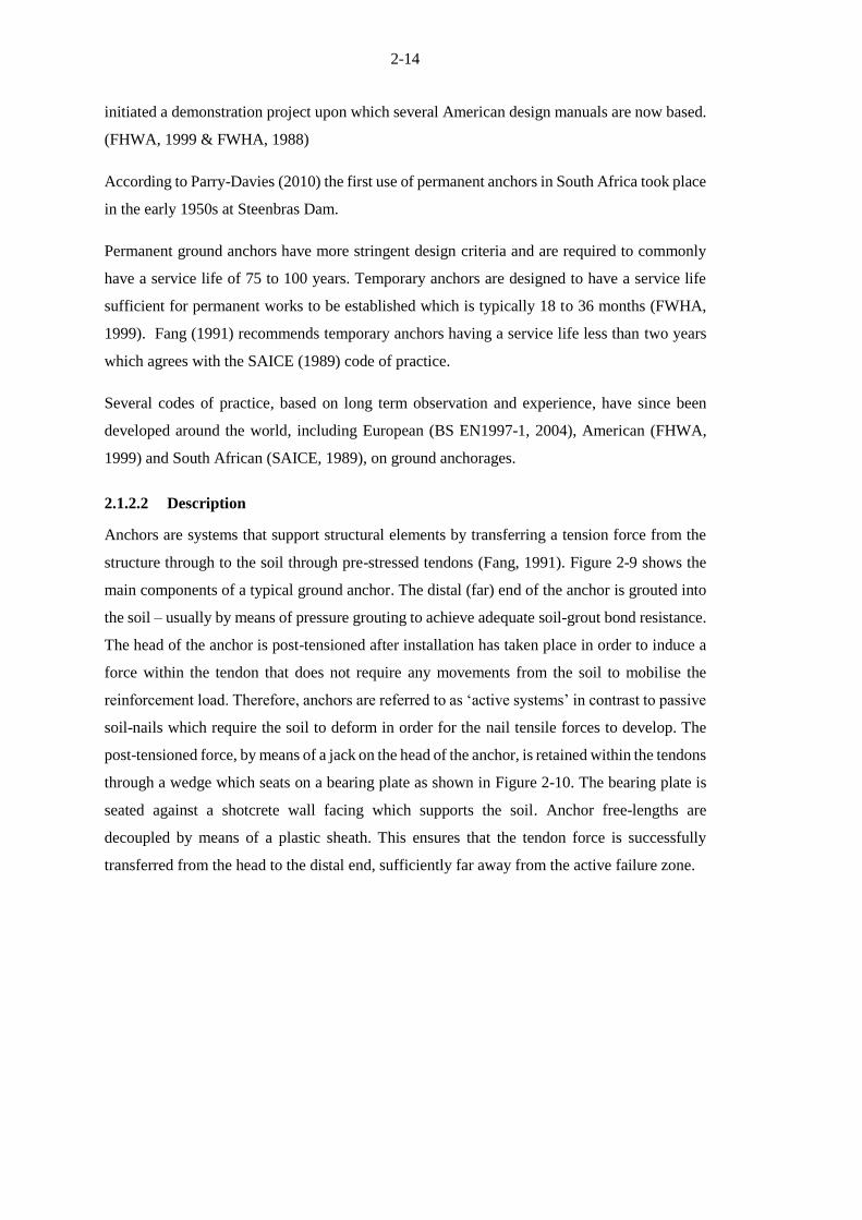
2.1.2.2 Description
Anchors are systems that support structural elements by transferring a tension force from the
structure through to the soil through pre-stressed tendons (Fang, 1991). Figure 2-9 shows the
main components of a typical ground anchor. The distal (far) end of the anchor is grouted into
the soil – usually by means of pressure grouting to achieve adequate soil-grout bond resistance.
The head of the anchor is post-tensioned after installation has taken place in order to induce a
force within the tendon that does not require any movements from the soil to mobilise the
reinforcement load. Therefore, anchors are referred to as ‘active systems’ in contrast to passive
soil-nails which require the soil to deform in order for the nail tensile forces to develop. The
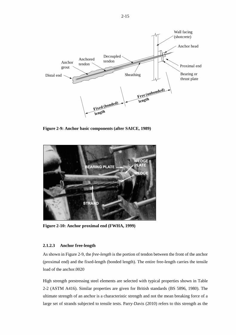
post-tensioned force, by means of a jack on the head of the anchor, is retained within the tendons
through a wedge which seats on a bearing plate as shown in Figure 2-10. The bearing plate is
seated against a shotcrete wall facing which supports the soil. Anchor free-lengths are
decoupled by means of a plastic sheath. This ensures that the tendon force is successfully
transferred from the head to the distal end, sufficiently far away from the active failure zone.
2-15
Figure 2-9: Anchor basic components (after SAICE, 1989)
Figure 2-10: Anchor proximal end (FWHA, 1999)
2.1.2.3 Anchor free-length
As shown in Figure 2-9, the free-length is the portion of tendon between the front of the anchor
(proximal end) and the fixed-length (bonded length). The entire free-length carries the tensile
load of the anchor.0020
High strength prestressing steel elements are selected with typical properties shown in Table
2-2 (ASTM A416). Similar properties are given for British standards (BS 5896, 1980). The
ultimate strength of an anchor is a characteristic strength and not the mean breaking force of a
large set of strands subjected to tensile tests. Parry-Davis (2010) refers to this strength as the
Anchor
grout
Distal end
Decoupled
tendon
Sheathing
Anchor head
Proximal end
Wall facing
(shotcrete)
Anchored
tendon
Bearing or
thrust plate

2-16
‘Guaranteed Ultimate Tensile Strength’. The FHWA (1999) uses the terminology of ‘Specified
Minimum Ultimate Strength’. To avoid confusion, this characteristic strength will be referred
to simply as the ‘ultimate strength’. FHWA (1999) and SAICE (1989) agree that the maximum
load on an anchor should not exceed 80% of the anchor ultimate strength during any phase of
testing, construction or service life.
The design load of an anchor, commonly known as the ‘working load’, is the force expected to
be carried by the tendon during its service life. Typically, the highest load an anchor carries
occurs during proof load testing. The proof load is between 1.25 and 1.5 times the working load
depending on the code of practice used and whether temporary or permanent anchorages are
applied. The maximum allowable working load is shown in Table 2-3. The working load is
factored by the allowable load on the anchor (80% of the ultimate strength) and the proof load
testing (125% – 150% of the working load). Therefore, for a temporary excavation, a designer
can specify a working load of 167kN per strand (ultimate strength ∙ 80% = working load ∙ 125%)
according to SAICE (1989) using ASTM A416 standard materials. In the past, lateral support
specialists have often opted for a conservative approach by specifying a working load of
150kN/strand for temporary works (Parry-Davies, 2010).
It must be understood that the working-, proof-, lock-off - and ultimate loads will differ and
must be specified according to the appropriate code of practice and in conjunction with the
manufacturer’s product specifications.
Table 2-2: Properties of 15-mm diameter prestressing steel strands (ASTM A416, Grade
270 metric 1860) from FHWA, 1999
Number of
15mm strands
Nominal Cross-
sectional area
(mm²)
Ultimate
Strength (kN)
Prestressing Force (kN)
80% 70% 60%
1 140 260.7 209 182 156
3 420 782.1 626 547 469
4 560 1043 834 730 626
5 700 1304 1043 913 782
7 980 1825 1460 1278 1095
9 1260 2346 1877 1642 1408
12 1680 3128 2502 2190 1877
15 2100 3911 3129 2738 2347
19 2660 4953 3962 3467 2972

2-17
Table 2-3: Comparison of maximum working load for different codes
Code of Practice
A. Proof Load
Testing
B. Maximum
Load
C. Maximum
Working Load
[B÷C]
D. Working Load
(% of Fworking) (% of Fultimate) (% of Fultimate) (kN per strand)
Temporary
FHWA, 1999 133 80 60 157
SAICE, 1989 125 80 64 167
Permanent
FHWA, 1999 150 80 53 139
SAICE, 1989 150 80 53 139
2.1.2.4 Anchor fixed-length
Fixed-lengths, also commonly known as bonded/grouted lengths, refer to the distal portion of
the anchor with adequate soil-grout interface strength to ensure that tensile loads from the
structure are transferred to the soil.
Several installation techniques have been used in the past depending on site soil type conditions,
restrictions and availability of equipment. Four main installation techniques of the fixed-lengths
are shown in Figure 2-11. Each installation technique differs on constructability and the soil-
grout bond resistance which determines the fixed-length anchorage capacity.
Type A: Straight shaft ground anchors are found within competent materials such as rock or
very stiff clays. Grouting is achieved by using a tremie pipe down boreholes which may or may
not include lining depending on the stability of the hole (FHWA, 1999).
Type B: Straight shaft pressure grouted anchors offer additional capacity due to the hole
enlargement caused by pressure. The increase in normal stress on the soil-grout interface due
to the confinement of the pressured grout also contributes to increasing the bond resistance
(FHWA, 1999). Pressures can be achieved by inserting a packer into the borehole isolating the
pressurised grout cavity. This type of anchoring is effective for soft fissured rocks but can be
successful for a range of cohesionless materials (SAICE, 1989).
Type C: Post-grouted anchors offer large soil-grout bond resistances increasing the available
capacity of the anchor. Multiple delayed grouting injections allows high pressure grout, in
excess of 1MPa, to hydrofracture or compact the initial grout which increases the effective area
of the soil-grout interface (SAICE, 1989).
Sequential grouting is often used by incorporating a special grout tube called a Tube-á-
Manchette (TAM) as shown in Figure 2-12. A TAM uses multiple packers to isolate chambers

2-18
and achieve the required pressures. Repetitive grouting flows through a series of rubber sealed
one way values (Fang, 1991). Post-grouted, high pressure anchors are often used in
cohesionless materials (SAICE, 1989).
Type D: Underreamed anchored are found within in stiff to very stiff cohesive deposits.
(SAICE, 1989).
Figure 2-11: Main types of grouted ground anchors (Littlejohn, 1990)

2-19
a. Pressure-grouted anchor b. T.A.M.
Figure 2-12: High pressure post-grouted anchors using a T.A.M system. Example of
Soletanche IRP anchor (Pfister et al. 1982)
Anchor pull-out resistance
The post-grouting technique results in a root/fissure system which interlocks with the adjacent
soil, substantially increasing the capacity of the anchor. In dense cohesionless soils the high
pressure grouting system causes a material to dilate when shear occurs, increasing the soil-grout
normal stress (Fang, 1991). To derive a theoretical basis for the pull-out resistance is difficult
and commonly the post-grouted fixed-length resistance is empirically derived from assuming a
uniform shear stress and the results of pull-out tests (SAICE, 1989).
Several authors have compiled anchor pull-out resistances based on the soil-grout interface
shear strength of the fixed-lengths. PTI (1996) recommend using soil-grout bond values as
shown in Table 2-4. Interface shear stress values are given for a range of soils for straight shaft
gravity and pressure grouted installation techniques (Type A & B). It is recommended by the
FHWA (1999) that these values be based on the initial drilling diameter although pressure
grouting might result in an increased effective diameter.
It is readily recognised that post-grouting (Type C) will significantly increase the shear strength
between the grout and soil of the fixed-length. Post-grouting in cohesive soils are estimated to
increase the bond strength by 20 -50% per reinjection phase with an upper limit of three phases
(FHWA, 1999).
The significant influence of grouting pressure on bond capacity is shown in Figure 2-13. For
cohesionless materials such as gravels and sands, Jorge (1969) indicates an approximate

2-20
increase in pull-out resistance of 6.1kN/m for every 100kPa increase in pressure. For a 6m
fixed-length, that is almost a 400kN increase in pull-out resistance for 1MPa increase in
grouting pressure.
Table 2-4: Typical ultimate bond stress for soil-grout interface along anchor fixed-
length (PTI, 1996)

2-21
Figure 2-13: Influence of grout injection pressure on ultimate bond capacity of anchors
(Jorge, 1969)
Anchor length
Anchor fixed-lengths are typically between 4.5 – 12m. Although it is admitted that only
moderate benefit is gained beyond 6m (FHWA, 1999). SAICE (1989) recommend that anchor
fixed-lengths are between 3 – 8m in cohesionless soils and 5 – 10m in cohesive soils.
Figure 2-14 shows the pull-out resistance of anchors against the length of the bond. Unless
special installation techniques are used, little benefit is gained for long anchors beyond 10 –
12m due to anchors not effectively transferring the load from the front of the fixed-length to
the back (distal) end (Fang, 1991).

2-22
Figure 2-14: Ultimate load holding capacity of anchors in cohesionless soils (After
Ostermayer and Scheele, 1977)
2.1.2.5 Construction sequence
The construction sequence of ground anchors is important towards the understanding the
loading experienced by individual anchors.
Figure 2-15 illustrates the top-down construction technique which is typically followed for the
installation of anchors in surface excavations. Often, before the excavation commences, a
vertical pile, referred to as a ‘soldier pile’ is installed. The soldier pile is a bearing element for
the anchors to effectively distribute the loads to the soil. The embedment depth of the soldier
pile also aids stability, especially for the excavation of the first row of anchors. After installation
of piles, excavation takes place to approximately 0.5m below the level of the first row of
anchors. A shotcrete face is applied with the thickness according to the design. Anchors are
installed with their fixed-lengths pressure-grouted. After the grout has set, according to SAICE
(1989), the anchors will be stressed to 125% of their working load for proof load testing (150%
for permanent anchors). The maximum working load is calculated based on the requirement
that the proof load testing may only be 80% of the ultimate load. Anchors are locked off at
110% of working load. 10% allows for short and long term losses. Different codes, such as
FHWA (1999), differ slightly from the values for proof load testing, maximum working loads
and the lock-off load. The excavation of the next phase will commence and the process is
repeated until the final level is achieved.

2-23
1. Soldier pile installation 2. Excavation to appropriate depth
3. Drilling, installation of anchor and
shotcrete (incl. anchor stressing)
4. Excavation of next phase
Figure 2-15: Top-down construction sequence of anchors (FWHA, 1999)
2.1.2.6 Embedded retaining walls and soldier pile lateral capacity
Stability of retained soil can be achieved or aided by using embedded structural elements. Three
common types of embedded walls increasing in complexity is shown Figure 2-16.
A cantilevered retaining wall (Figure 2-16a) requires substantial embedment depth as the
stability is dependent on only the resistance created by the subgrade and the structural capacity
of the wall.
A single tie-back (Figure 2-16b) is another common situation of an embedded retaining wall.
A cantilevered retaining wall is combined with additional support near the top of the wall. The
reinforcement could take the form of a ground anchor, prop or a dead-man anchor. Depending
on the depth of embedment, an assumption is made about the fixity, which renders the problem
statically determinate. The pressure diagrams, anchor forces and bending moments in the wall
can be computed. In general, two types of analysis exist depending on the embedment depth of
the piles: free-earth support and fixed-earth support.
With free-earth support conditions, the assumption is made that the depth of penetration is
sufficient to prevent instability by passive failure, i.e. translation. However, rotation about the
toe of the embedded wall is not prevented. The consequence of this method is that there is not

2-24
a reversal of bending moment below the subgrade. The pile can be seen as a vertical beam
spanning two simple supports being the anchor/prop and the subgrade. Rowe (1952) calculated
allowable moment reductions due to redistribution for sheet piles using the free-earth support
method. Fixed-earth conditions occur if there is sufficient embedment depth resulting in no
rotation at toe of the wall. The soil below the subgrade will contain both active and passive
pressures and a reversal in bending moment of the piles will occur.
With a multi-level anchored system (Figure 2-16c), the problem becomes significantly more
complex. The forces and moments depend on the relative strength and stiffness of the soil and
structural elements. Additionally, the construction sequence will play a significant role (SAICE,
1989). The pressure distribution cannot easily be calculated. Semi-empirical methods exist such
as pressure envelopes adapted from Terzaghi & Peck (1967) and Peck (1969) which are
recommended by FHWA (1999).
Due to soil variability and strain incompatibilities between active and passive movements, a
FoS is applied when calculating the embedment depth. Different codes and authors use different
factors of safety, such as 1.2 (Gunaratne, 2014) and 1.5 (FHWA, 1999), with regard to passive
resistance.
a. Cantilever pile b. Single anchored pile c. Multi-level anchored wall
Figure 2-16: Common embedded pile support systems (Gunaratne, 2014)
Broms’ Method
Soldier piles are often used in combination with multi-level anchored systems as briefly
discussed in Section 2.1.2.5. Solider piles can be embedded below the surface of the final
excavation. This will cause additional passive resistance as a function of the depth of the pile.
Broms (1965) developed simple analytical solutions to evaluate the lateral capacity of piles in
drained and undrained conditions. Broms stipulated that the lateral capacity of a pile during
undrained conditions will be approximately nine times the undrained shear strength across the
pile width, b, as shown in Figure 2-17a.

2-25
In cohesionless materials, when drained conditions apply, the lateral capacity can be taken as
three times the passive pressure as shown in Figure 2-17b. Several assumptions are made,
primarily, that (1) the active pressure behind the pile below the excavation depth can be ignored
due to the forward motion and (2) that the load spread in the front of the pile will be three times
the pile width, b (Gunaratne, 2014).
a. Undrained condition b. Drained condition (cohesionless,
long term cohesive)
Figure 2-17: Broms method for evaluating the ultimate lateral capacity of embedded
piles (FHWA, 1999)
Wang-Reese Method
Wang and Reese (1986) developed another common method for calculating the ultimate lateral
capacity of piles. The Wang-Reese Method considers three potential failure mechanisms
dependent on the depth of embedment, pile width and pile spacing. The Wang-Reese Method
considers the minimum of:
1. 3-D wedge failure in front of the pile as shown in Figure 2-18
2. Overlapping wedges due to close pile spacing
3. Plastic flow around piles due to great embedment depth
Figure 2-19 shows the passive resistance against the depth of embedment for Broms and Wang-
Reese methods of cohesionless soils i.e. drained condition. In these plots, a FoS of 1.5 is
included. It can be seen that for embedment depths below 1.5m, Broms’ method is more
conservative.

2-26
a. Wedge failure in clay b. Wedge failure in sand
Figure 2-18: Wang-Reese failure wedge in sands and clays (FHWA, 1999)
Figure 2-19: Broms and Wang-Reese comparison for lateral capacity of solider piles
(FWHA, 1999)

2-27
2.2 METHODS OF ANALYSIS
The previous section described two methods of lateral support: soil-nails and anchors. Several
methods could be employed to analyse the stability of these systems. In this section, some of
these methods of analysis are discussed.
2.2.1 Selected soil mechanics aspects
Although it is beyond the scope of this dissertation to present an in-depth study of the broad
topic of soil mechanics, an overview of some components relevant to the project scope is
important.
2.2.1.1 Plane strain
For convenience of calculation, slope stability programs are reduced to two dimensions (2-D)
by assuming plane strain conditions, i.e. the lateral out of plane strains are zero. This assumption
would approximate a slope / excavation of infinite length. However, even if the cross-section
is uniform, rarely do entire slopes fail to represent plane strain conditions. All embankments
have ‘end-effects’ that provide additional resistance due to the 3-D mode of failure. Azzouz &
Baligh (1982) developed a 3-D slope stability model and found that a 3-D failure modes
increase the conventional plane strain FoS by 5 – 15% due to the end-effects. Mollahasani
(2015) found that the FoS could be increased by 25% by comparing a 2-D and 3-D analyses of
quay walls.
Numerical techniques have been developed for 3-D analysis but remain costly and relatively
new. For situations, such as rectangular box excavations, a plane strain analysis, which does
not take into account the resistance of the end effects, will give conservative results. Duncan
(1996) reviews several authors and finds that 2-D plane strain analyses, are in all cases
conservative.
2.2.1.2 Horizontal soil pressure
In-situ stresses
For a retaining wall with sufficient movement towards the excavation, the stress state in the soil
mass will tend towards Rankine’s active condition. For movement opposing the instability, with
enough force, the passive pressures will be reached. Conventionally, Rankine’s active and
passive pressures are the minimum and maximum pressures within a soil continuum
respectively. However, the horizontal pressures within soil, in its in-situ state, lies somewhere
between these pressures (a reduction in pressure below the active pressure is possible locally in

2-28
flexible systems due to arching). The horizontal pressure is defined in terms of the stress ratio,
K, also referred to as the coefficient of lateral earth pressure.
Coefficient of lateral earth pressure: 𝐾 = 𝜎ℎ′
𝜎𝑣′ (2.5)
Since the vertical stress, σv, is easily determined by the overburden pressure, the horizontal
stress, σh, is specified in terms of the depth of the soil and the coefficient K. The lateral earth
pressure for the in-situ soil is referred to as the at-rest earth pressures. The name is derived from
the fact that if no movement occurs there will be no deviation from the in-situ stress.
The in-situ stresses, which are largely a function of the stress history and geology, cannot be
derived from first principles for a natural soil deposit. The at-rest earth pressure coefficient, K0,
could be determined from advanced triaxial testing, dilatometer tests, pressure-meter tests or
indirect methods such as CPTu tests (SAICE, 1989).
Several authors have published data on the determination and prediction of the value of the in-
situ earth pressures (Kulhawy & Mayne, 1990; Kulhawy et. al. 1989, Lambe & Whitman,
1969). Typical values for K0 by Whitlow (1990) are given in Table 2-5. Perhaps the most well-
known empirical relationship, derived by Jaky (1944), for normally consolidated sands is
shown in Equation (2.6).
Normally consolidated sands: 𝐾0 = 1 − sin𝜙′ (2.6)
Theoretically, for a condition where no lateral strain can occur and compression can only take
place in the vertical direction, K0 can be derived as a function of the Poisson’s ratio, v’. The
coefficient of lateral earth pressure for one dimensional compression is shown in Equation
(2.7). This value for K0 is adopted by numerical software such SIGMA/W (2007).
1-Dimensional compression: 𝐾0 =𝑣′
1 − 𝑣′ (2.7)
In over-consolidated soils, Jaky’s correlation has been adapted by Schmidt (1966) to take into
account the over-consolidation ratio (OCR) as shown in Equation (2.8).
Over-consolidated soils: 𝐾0 = 1 − sin𝜙′ √𝑂𝐶𝑅 (2.8)
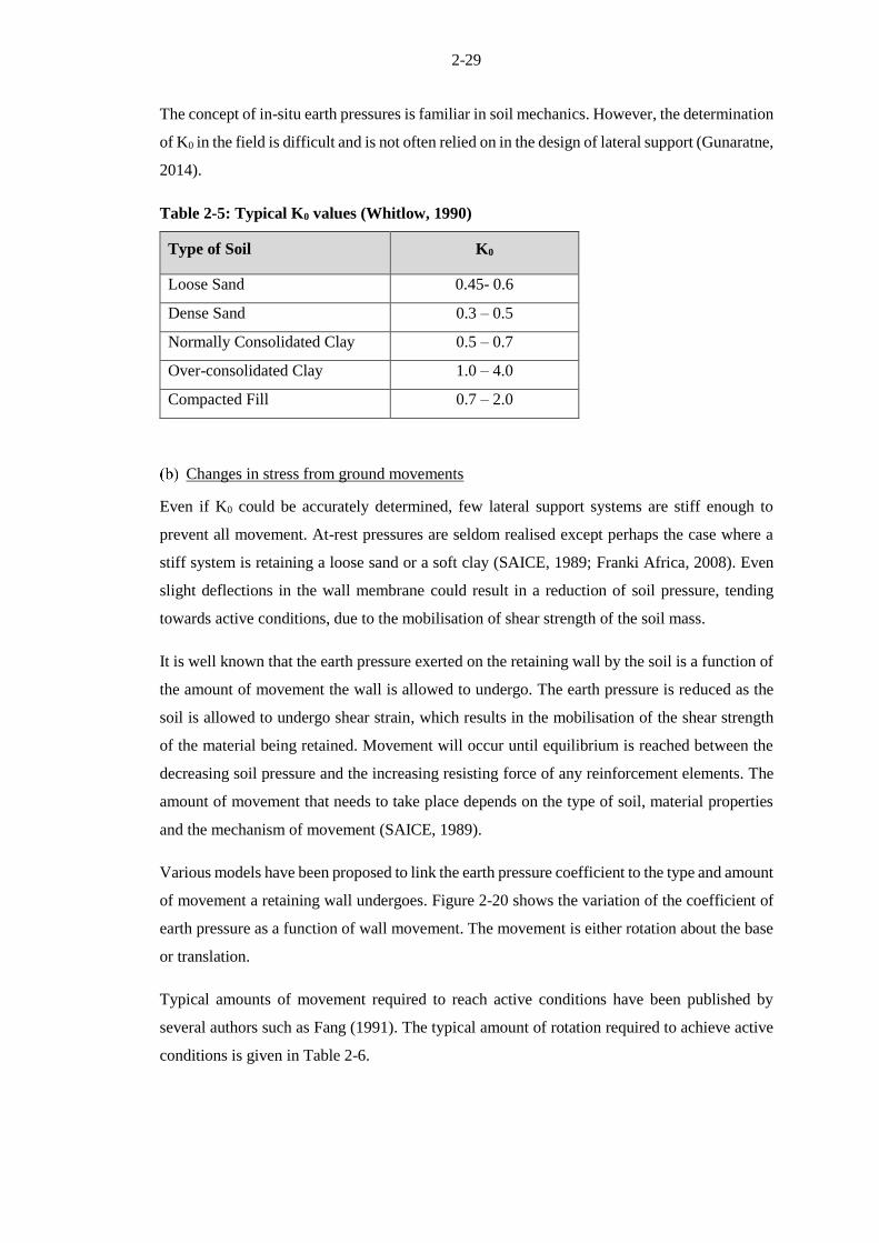
2-29
The concept of in-situ earth pressures is familiar in soil mechanics. However, the determination
of K0 in the field is difficult and is not often relied on in the design of lateral support (Gunaratne,
2014).
Table 2-5: Typical K0 values (Whitlow, 1990)
Type of Soil K0
Loose Sand 0.45- 0.6
Dense Sand 0.3 – 0.5
Normally Consolidated Clay 0.5 – 0.7
Over-consolidated Clay 1.0 – 4.0
Compacted Fill 0.7 – 2.0
Changes in stress from ground movements
Even if K0 could be accurately determined, few lateral support systems are stiff enough to
prevent all movement. At-rest pressures are seldom realised except perhaps the case where a
stiff system is retaining a loose sand or a soft clay (SAICE, 1989; Franki Africa, 2008). Even
slight deflections in the wall membrane could result in a reduction of soil pressure, tending
towards active conditions, due to the mobilisation of shear strength of the soil mass.
It is well known that the earth pressure exerted on the retaining wall by the soil is a function of
the amount of movement the wall is allowed to undergo. The earth pressure is reduced as the
soil is allowed to undergo shear strain, which results in the mobilisation of the shear strength
of the material being retained. Movement will occur until equilibrium is reached between the
decreasing soil pressure and the increasing resisting force of any reinforcement elements. The
amount of movement that needs to take place depends on the type of soil, material properties
and the mechanism of movement (SAICE, 1989).
Various models have been proposed to link the earth pressure coefficient to the type and amount
of movement a retaining wall undergoes. Figure 2-20 shows the variation of the coefficient of
earth pressure as a function of wall movement. The movement is either rotation about the base
or translation.
Typical amounts of movement required to reach active conditions have been published by
several authors such as Fang (1991). The typical amount of rotation required to achieve active
conditions is given in Table 2-6.

2-30
Table 2-6: Rotation required about base for mobilisation of active pressures (SAICE,
1989)
Soil type Rotation about base (Δ/H)
Active Passive
Dense Non-Cohesive 0.0005 – 0.001 0.002 – 0.02
Loose Non-Cohesive 0.002 – 0.005 0.006 – 0.15
Stiff Cohesive 0.002 – 0.01 0.01 – 0.02
Soft Cohesive 0.005 – 0.02 0.02 – 0.04
Figure 2-20: Relationship between wall movement and earth pressure for ideal cases of
walls “wished into place” (Fang, 1991).
Rotation about the top, rotation about the base and translation of the wall are all common
possible movement mechanisms. The earth pressure distributions for the various movement
mechanisms are shown in Figure 2-21. It is important to note that no matter the type of
movement the earth pressure will, given enough strain, reach the active state as the soil mass
yields.
Parallel translation requires around 2-3 times more movement than rotation about the base for
active conditions to be achieved. Rotation about the top of the retaining wall requires up to 5
times as much movement as rotation about the base. During Parallel translation or rotation

2-31
about the top of the wall, an ‘arching active’ pressure distribution develops with a thrust
approximately the magnitude of active conditions.
a. Fixed wall b. Rotation about base
c. Rotation about top d. Translation
Figure 2-21: Reduction in earth pressure due to movement mechanism (Mc Gown et al.
1987)
Allowable movements in soil-nailed and anchored structures
The design philosophy of lateral support is to prevent failure and provide sufficient margin of
safety to adequately satisfy variability and serviceability considerations (Lai Sang & Scheele,
1999; BS8006, 1995). However, in many cases serviceability considerations could be as
onerous as failure conditions (Simpson & Driscoll, 1998). Currently design procedures are
focused on stability calculations and only guidelines are recommended for serviceability
requirements (SAICE, 1989; Clouterre, 1991).
Soil-nails have the distinct property of being passive inclusions which means soil-nails need
movement to mobilise their resistive forces.
2-32
One of the primary concerns with movement is damage to adjacent structures. Well known
limits on angular distortion have been given by Bjerrum (1963). SAICE (1989) recommend
limiting the maximum horizontal movement of a retaining wall in urban areas to 35mm. Several
databases on movements of retaining structures has been published (Long, 2001; SAICE,
1989), however, the scatter remains large. Also, relating stability calculations at failure
conditions to movements at working conditions seems to be erroneous.
2.2.1.3 Water pressures
Many shotcrete retaining wall systems are designed with vertical drains terminating at weep
holes which result in a significant decrease in lateral pressure if a water table is present.
However, since the stability is determined as a function of the effective stress on the rupture
surface, as long as the water pressure encroaches on the active zone within the retained material,
an increase in lateral pressure will be experienced. This is true even if the back of the retaining
wall is completely dry due to fully operational drains. In the case of embedded walls, a seepage
gradient will result in a decrease in passive pressure in front of the wall (SAICE, 1989).
The presence of water will decrease stability. However, for the purposes of this report the water
table was assume to be sufficiently far below the excavation to be disregarded.
2.2.1.4 Elasticity and plasticity
Elasticity and plasticity theories are commonly applied to model many civil engineering
materials. Perhaps the simplest example of these theories is seen in the tensile failure of a steel
bar. As the bar is tensioned, the load increases in direct proportionality to the increase in length.
The load is often described as a stress and the increase in length as strain. The direct
proportionality between stress and strain is not common to soils and therefore soils are
described as non-linear materials.
Once the load on the bar is released, the bar should approximately shrink back to its original
length. Elastic behaviour is such that no permanent deformation of the material takes place. If
the bar is further tensioned, at some point, permanent irrecoverable deformation will start to
take place and from this point the material will behave plastically. The point at which plastic
deformation starts occurring is called the yield point which needs to be defined in plasticity
theory. In a steel tensile test, the point of yielding is easy to define. In soils, however, it is not
as easy to identify the onset of plastic deformation. Furthermore, soils are rarely loaded in one-
dimensional manner. In two dimensions the yield point becomes a yield curve and in three
dimensions the yield curve will become in a yield surface. Figure 2-22 shows a yield surface
for a Mohr-Coulomb failure criterion often used for soils. Where σ1, σ2 and σ3 are the principal
stresses in three dimensions.

2-33
Figure 2-22: Mohr-Coulomb yield surface (PLAXIS, 2016)
Hardening
One of the problems in plasticity theory is determining subsequent post yield surfaces. This
post-yielding response of the material is described by the hardening law which gives the rule
of the evolution of yield surfaces during plastic deformation (Chen & Liu, 1990). Figure 2-23
shows typical load deformation curves for strain hardening and softening materials. A strain
hardening material’s yield point increases as plastic deformation takes place. A strain softening
material will reach the yield point which is the maximum load that it can carry. If the stress-
strain curve is load controlled, brittle failure will occur.
a. Strain hardening b. Strain softening
Figure 2-23: Strain hardening or softening materials (Clayton et al. 2013)
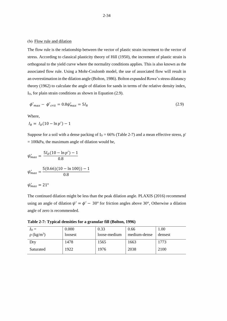
2-34
Flow rule and dilation
The flow rule is the relationship between the vector of plastic strain increment to the vector of
stress. According to classical plasticity theory of Hill (1950), the increment of plastic strain is
orthogonal to the yield curve where the normality conditions applies. This is also known as the
associated flow rule. Using a Mohr-Coulomb model, the use of associated flow will result in
an overestimation in the dilation angle (Bolton, 1986). Bolton expanded Rowe’s stress dilatancy
theory (1962) to calculate the angle of dilation for sands in terms of the relative density index,
ID, for plain strain conditions as shown in Equation (2.9).
𝜙′𝑚𝑎𝑥 − 𝜙′𝑐𝑟𝑖𝑡 = 0.8𝜓𝑚𝑎𝑥′ = 5𝐼𝑅 (2.9)
Where,
𝐼𝑅 = 𝐼𝐷(10 − ln𝑝′) − 1
Suppose for a soil with a dense packing of ID = 66% (Table 2-7) and a mean effective stress, p'
= 100kPa, the maximum angle of dilation would be,
𝜓𝑚𝑎𝑥′ =
5𝐼𝐷(10 − ln𝑝′) − 1
0.8
𝜓𝑚𝑎𝑥′ =
5(0.66)(10 − ln 100)) − 1
0.8
𝜓𝑚𝑎𝑥′ = 21°
The continued dilation might be less than the peak dilation angle. PLAXIS (2016) recommend
using an angle of dilation 𝜓′ = 𝜙′ − 30° for friction angles above 30°, Otherwise a dilation
angle of zero is recommended.
Table 2-7: Typical densities for a granular fill (Bolton, 1996)
ID = 0.000 0.33 0.66 1.00
ρ (kg/m3) loosest loose-medium medium-dense densest
Dry 1478 1565 1663 1773
Saturated 1922 1976 2038 2100

2-35
Linear elastic perfectly-plastic materials
In the Mohr-Coulomb model, a typically assumed stress-strain curve is initially linear elastic,
then perfectly-plastic as shown in Figure 2-24. The gradient of the elastic portion is defined by
Young’s modulus, E', and remains linear according to Hooke’s law. The yield point, where
collapse occurs is defined by with Mohr-Coulomb failure envelope. In three dimensions,
yielding will occur if the stress path touches the yield surface.
The implication is that neither non-linearity of soil stiffness nor working hardening/softening
are modelled.
The stiffness (E' and v') and strength parameters (ϕ' and c') are commonly known to engineers.
The Mohr-Coulomb model, amidst its simplifications, is currently the most widely used model
in geotechnical practice (ICE, 2012).
Typical stiffness values for a variety of soil types are given in Table 2-8 and Table 2-9 for
Young’s modulus and Poisson’s ratio respectively.
Figure 2-24: Linear elastic perfectly-plastic (Clayton et al. 2013)

2-36
Table 2-8: Typical range of values of Young's modulus (Bowles, 1996)
Soil Modulus, E' (MPa)
Clay
Very soft 0.3 - 3
Soft 2 - 4
Medium 4.5 - 9
Hard 7 - 20
Sandy 30 - 42.5
Glacial fill 10 - 160
Loess 15 - 60
Sand
Silty 5 - 20
Loose 10 - 25
Dense 50 - 100
Sand and gravel
Dense 80 - 200
Loose 50 - 140
Shales 140 - 1400
Silt 2 - 20
Table 2-9: Typical range of values of Poisson’s ratio (Bowles, 1996)
Soil Poisson’s Ratio, v'
Clay, saturated 0.4 - 0.5
Clay, unsaturated 0.1 - 0.3
Sandy clay 0.2 - 0.3
Silt 0.3 - 0.35
Sand (dense) 0.2 - 0.4
Coarse (void ratio = 0.4 - 0.7) 0.15
Fine-grained (void ratio = 0.4 - 0.7) 0.25
Rock 0.1 - 0.4
Loess 0.1 - 0.3
Ice 0.36
Concrete 0.15

2-37
2.2.2 Plastic analysis
Plastic limit analysis is concerned with methods for calculating the collapse load for structures
in a direct manner. Although limit analysis is a fairly new field, the idealisation of associated
flow in the framework of a perfectly-plastic material makes it a mathematically rigorous model
that was been firmly established as a practical tool for design engineers (Chen & Liu, 1990).
Real soils are of course not perfectly-plastic at collapse but rather work hardening or softening.
That is, the soil increases or decreases in strength post yielding. The dramatic idealisation of
perfect-plasticity must be viewed with caution to prevent improper interpretation of results
(Chen & Liu, 1990).
Early application of plasticity theory was almost entirely attributed to the limit analysis of mild
steel which behaves as a perfectly-plastic material because of its ductile nature (Prager &
Hodge, 1951). Hill (1950) and Drucker & Prager (1952) extended the theory of metal plasticity
to soils. The Mohr-Coulomb failure criterion was seen as a special case of the Tresca failure
envelope (a yield criterion associated with metals). One of the main problems in identifying the
onset of irreversible plastic deformation is the overestimation of the dilation due to the use of
the associated flow rule. The initial theories were therefore extended to non-associated flow,
where the increment of plastic strain need not be normal to the yield surface.
2.2.2.1 Upper and lower bounds to collapse loads
Amidst the simplifications, soils are often described to behave in an elastic perfectly-plastic
manner. In order to satisfy the plastic theory of soil, four requirements have to be met:
1. Equilibrium is satisfied in the elastic and plastic zones throughout the deformation
stages;
2. Strains are compatible;
3. Elastic stresses and strains relate to one another by Hooke’s law; and
4. Plastic stresses occur on the yield surface of the material. And the corresponding plastic
strain vectors occur normal to the yield surface. This means that the normality condition
applies and the associated flow rule is applicable.
One can simplify the calculations of an elastic perfectly-plastic material by considering the
collapse state of that material. By considering the collapse state the initial preliminary elastic
partly-plastic stages are ignored (Atkinson, 1993). It is self-evident that analysing the collapse
loads corresponds to analysing the strength of the structure (Calladine, 2000). In many
engineering applications, this is what is needed.

2-38
The collapse of a structure is viewed by the ‘bounds theorems’ (note, that when a ‘structure’ is
mentioned it can refer to a soil continuum and not necessarily an object as typically considered
in structural engineering). The bounds theorems form an integral part of plasticity theory and
are hard to concisely describe without the use of examples (Calladine, 2000). Two approaches
exist in the bounds theorems which result in the so-called upper and lower bound theory.
The upper and lower bounds represent two extremes on the spectrum of predicting the collapse
load of any structure. The true load that causes collapse will be somewhere between the bounds
of the upper and lower predictions. It follows that if the upper bound is equal to the lower bound
solution, the exact collapse load has been calculated.
Lower bound
The ‘equilibrium’ approach satisfies the equations of equilibrium throughout the structure. At
the same time, nowhere within the structure is the yield condition violated. This is termed a
‘statically admissible stress field’. The collapse load calculated by this approach is always on
the low side (if not equal) of the actual collapse load. This is known as the lower bound collapse
load. Nowhere is the deformation or compatibility of strains considered (Calladine, 2000).
Definition: If there is a set of external loads and the state of stress at no point exceeds the failure
criterion of the material, collapse cannot occur. This is the lower bound of the true collapse
load.
Another way of stating the lower bound collapse load is that lower collapse loads cannot cause
plastic flow of the structure.
Upper bound
The second approach is known as the ‘geometric’ approach where the mode of deformation is
considered by viewing a collapse mechanism. An energy balance is applied by virtual work and
at no point is equilibrium considered. This is termed a ‘kinematically admissible velocity field’.
The collapse load calculated from this approach is on the high side (if not the same) of the
actual collapse load (Calladine, 2000). Equilibrium is not considered and the upper bound
collapse mechanism need not be the true collapse mechanism.
In order to successfully compute upper bound solutions, some sort of collapse mechanism needs
to be added. In a steel beam, plastic analysis is applied by removing redundancies to the point
of rendering the beam statically unstable. The same can be accomplished with a soil continuum
by adding slip planes (Atkinson, 1993). Slip planes may be either straight lines or circular arcs
or even a combination of the two.

2-39
Definition: If there is a set of external loads and plastic collapse mechanism such that in an
increment of deformation the work done by the external loads equals the work done by the
internal stresses, collapse must occur. This is the upper bound of the collapse load.
Undrained vertical excavation bounds
Evaluating the maximum unsupported height of a vertical face can be solved by considering
the lower and upper bound plasticity solutions (Verruijt, 2001).
The lower bound solution stipulates that nowhere within the stress field may the yield criterion
be violated. Thus, if critical element is taken at the toe of the excavation, the maximum height
be calculated. Consider a vertical cutting with undrained shear strength, cu, and unit weight, γ.
The lower bound to the maximum unsupported face height, Hmax, can be calculated as,
𝐻𝑚𝑎𝑥 = 2𝑐𝑢𝛾 (2.10)
A higher lower bound value can be found on the premise of more complex stress fields. Pastor
et al. (1978) found,
𝐻𝑚𝑎𝑥 = 3.64𝑐𝑢𝛾
(2.11)
A higher value than Pastor’s calculation for lower bound has not yet been found (Verruijt,
2001).
The upper bound solution can be obtained by considering a linear failure wedge and the
maximum height can be calculated by the principle of virtual work as,
𝐻𝑚𝑎𝑥 = 4𝑐𝑢γ
(2.12)
Using Fellenius’ method of circular slip planes, Heyman (1973) gives an upper bound solution
of,
𝐻𝑚𝑎𝑥 = 3.83𝑐𝑢γ
(2.13)
A lower value has not been found. Thus, the true collapse load is somewhere within the lower
and upper bound calculations as shown in Equation (2.14).
3.63𝑐𝑢γ
≤ 𝐻𝑚𝑎𝑥 ≤ 3.83𝑐𝑢γ
(2.14)

2-40
It has to be noted that even with a simple problem of a vertical cut face with a homogenous soil
with a constant defined cu and γ values the upper and lower bound values still differ.
2.2.3 Limit equilibrium methods
Stress analyses in geotechnical engineering are broadly divided in two categories: stability or
serviceability. As mentioned earlier, the scope of this dissertation is limited to the stability
calculations of lateral support systems. In considering stability problems, of primary concern is
the limiting load a certain configuration can sustain before collapse. In practice solutions to the
collapse loads are often obtained by simple statics by assuming failure surfaces comprising of
various simple shapes and using a failure criterion. This is known as the limit equilibrium
method (Chen & Liu, 1990).
The limit equilibrium method predates plasticity methods for earth pressure problems and has
been in use for over 200 years. Coulomb first introduced the limit equilibrium method in 1773
to calculate the force of a fill on a retaining wall. Rankine, later in 1857, extended the theory to
an infinite body and developed the earth pressure theories. Subsequent developments by
Fellenius (1936), Terzaghi (1943) and others have made the limit equilibrium method a well
utilised tool for stability calculations by practicing engineers.
The limit equilibrium method combines features of the upper and lower bound methods found
by plasticity theory as discussed in the previous section. The limit equilibrium method is like
the upperbound method in that it considers a mode of deformation and follows the lower bound
method by ensuring equilibrium on a particular slip plane. Although there is no proof that the
limit equilibrium method leads to the correct collapse loads, experience has shown that the
method gives accurate solutions (Atkinson, 1993; Clayton et al. 2013). As with the upper bound
solutions, strikingly, the limit equilibrium method gives reasonable solutions no matter the
complexity of the geometry (Chen & Liu, 1990).
Using the limit equilibrium method, an arbitrary mechanism of collapse can be constructed with
simple slip lines – straight lines, circular arcs, log-spirals or any other slip lines. A requirement
for the limit equilibrium method is that each component (or shape) of the mechanism is in
equilibrium and that the whole mechanism is also in equilibrium. Generally, the mechanism is
varied to find the critical collapse load (Atkinson, 1993).
The limit equilibrium method might have some commonalities with the upper and lower bound
methods, however, some important differences and restrictions exist. With the upper bound
method, there are restrictions on the shape of the slip lines specific to drained and undrained
loading. For the lower bound method, it is required to examine the stress throughout the
2-41
continuum and show that the stress doesn’t exceed the yield criterion at any location. With the
limit equilibrium method, the equilibrium of forces is considered only on the boundaries of the
selected slip lines.
The limit equilibrium methods use the concept of a perfectly-plastic material. It neglects the
stress-strain relationships which is an essential part to the continuum mechanics of deformable
solids (Chen & Liu, 1990).
According to Fang (1991), the stability, in terms of FoS, of soil-nailed and anchored lateral
support systems are traditionally analysed using limit equilibrium methods. Translational or
rotational failure is assessed along potential sliding surfaces. Sliding wedges are often used due
to their simplicity. Slope stability procedures such as the method of slices have incorporated
reinforcement loads from anchors or soil-nails to assess the stability. Specialist software for
planar and multiple wedges, circular failure surfaces and the method of slices has been
developed and are common in practice (Clayton et al. 2013).
2.2.3.1 Sliding wedge method
A Coulomb failure wedge (1773) is one of the simplest limit equilibrium calculations. The
sliding wedge method can consist of a single or multiple wedges as long as the wedges are in
equilibrium and the system as a whole is also in equilibrium (Atkinson, 1993; Clayton et al.
2013).
For soil-nails, the German Method (Stocker et al. 1979; Gässler & Gudehus, 1981) uses a
bilinear sliding surface. The bilinear wedge method has also been simplified into a single wedge
(Das, 1999; Sheahan & Ho, 2003). The French Method (Schlosser, 1983) is not common since
the consensus of considering only tension and not shear in soil-nails.
For anchors, Kranz’s Method (1953), generalised by Broms (1968), assesses a bilinear sliding
wedge. However, the method is difficult to apply to multi-level anchored systems as the slip
surface is predefined along an anchor midpoint. Cheney (1984) recommends assessing the
stability of anchors using Rankine’s failure surface at an angle of 45°+ ½ϕ' above the horizontal.
One of the key differences between the methods is the definition of the Factor of Safety (FoS).
Some methods, define the factor of safety in terms of the reinforcement capacity. Other methods
place an emphasis on factoring the soil shear strength parameters. This point is further discussed
in Section 2.3.

2-42
Single wedge
A single Coulomb failure wedge can be varied at different failure angles to obtain the critical
failure surface, i.e. the failure surface with the lowest FoS. Sheahan & Ho (2003) have shown
with two case histories that trial wedge method can be successfully used to calculate the stability
of soil-nailed structures.
A single planar wedge considers a rigid body with a linear failure plane. Figure 2-25 shows
the forces acting on a single trial wedge. The weight of the wedge, W, can include a surcharge
which is not shown. Both soil-nails and anchors are considered as tension reinforcement, T.
The tension force is taken as the maximum force available behind the failure plane – this is
governed by either pull-out resistance or yielding of each individual inclusion. The resistance
is caused by the reaction force, R, resulting from friction, and any cohesion, C, along the failure
plane.
a. Forces acting on a single trial wedge b. Force polygon
Figure 2-25: Single trial wedge method
Double wedge
The same approach can be followed for multiple wedges as for the single wedge method
discussed above. In fact, for soil-nails, the double wedge method predates the planar single
wedge method. The method for soil-nails is based on the German Method (Gässler & Gudehus,
1981; Gässler, 1988).
CW
ϕ'
RT
β
β
α
R
T
W
C

2-43
Consider the forces on a double wedge failure mechanism as shown Figure 2-26. The influence
of cohesion has been ignored for clarity. The double wedge analysis works on the premise that
the two wedges are rigid blocks which are in equilibrium with themselves and the external
system. The contribution from reinforcement is only evaluated behind the failure surface and
not internally. The tension force can be from soil-nails or anchors. The tension reinforcement,
in this case, is shown to only contribute to the stability of the lower block. Gässler and Gudehus
(1981) have shown, to obtain the lowest FoS, the angle at which the upper wedge fails (No.1)
is 45°+ϕ'/2 above the horizontal. Software packages such as SNAIL (CALTRANS, 1992) are
available to analyse a double wedge failure mechanism.
A lower interwedge friction angle will produce more conservative results. Ingold (1995),
following calibration with Caquot and Kerisel (1948), suggests that an interwedge angle of ½ ϕ'
be used. Clayton et al. (2013) simplifies the procedure by assuming the interwedge failure to
be vertical and ignoring interwedge forces.
The angles and positions of the failure planes can be varied to obtain the critical slip surface as
with the single trial wedge method.
a. Forces acting on a double wedge b. Force polygon
Figure 2-26: Double trial wedge method
W1
ϕ'
ϕ'
α
T2
W2
R2
R1
ϕ'
R12
R21
W1
W2
R2
T2
R1
R12
R21
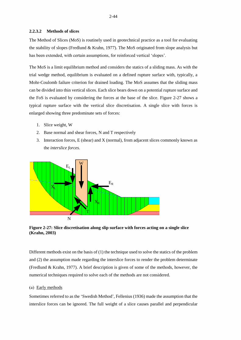
2-44
2.2.3.2 Methods of slices
The Method of Slices (MoS) is routinely used in geotechnical practice as a tool for evaluating
the stability of slopes (Fredlund & Krahn, 1977). The MoS originated from slope analysis but
has been extended, with certain assumptions, for reinforced vertical ‘slopes’.
The MoS is a limit equilibrium method and considers the statics of a sliding mass. As with the
trial wedge method, equilibrium is evaluated on a defined rupture surface with, typically, a
Mohr-Coulomb failure criterion for drained loading. The MoS assumes that the sliding mass
can be divided into thin vertical slices. Each slice bears down on a potential rupture surface and
the FoS is evaluated by considering the forces at the base of the slice. Figure 2-27 shows a
typical rupture surface with the vertical slice discretisation. A single slice with forces is
enlarged showing three predominate sets of forces:
1. Slice weight, W
2. Base normal and shear forces, N and T respectively
3. Interaction forces, E (shear) and X (normal), from adjacent slices commonly known as
the interslice forces.
Figure 2-27: Slice discretisation along slip surface with forces acting on a single slice
(Krahn, 2003)
Different methods exist on the basis of (1) the technique used to solve the statics of the problem
and (2) the assumption made regarding the interslice forces to render the problem determinate
(Fredlund & Krahn, 1977). A brief description is given of some of the methods, however, the
numerical techniques required to solve each of the methods are not considered.
Early methods
Sometimes referred to as the ‘Swedish Method’, Fellenius (1936) made the assumption that the
interslice forces can be ignored. The full weight of a slice causes parallel and perpendicular
W
N
T
ER
XR
XL
EL

2-45
components which depend on the angle of the rupture surface at the base. However, this method
does not ensure force equilibrium between slices. The method underestimates the FoS in the
region of 5-20% compared to more complex methods and can be out with as much as 60%
(Craig, 2004; Whitman & Bailey, 1967).
Bishop’s simplified approach (Bishop, 1955) extended the MoS and assumed that the interslice
forces are horizontal and therefore interslice shear forces are omitted. The formulation cannot
be arranged to solve for the FoS explicitly, however, an iterative procedure, by initially guessing
the FoS, can be followed. The error caused by using Bishop’s method in most cases is less than
2% and is in extreme cases unlikely to be higher than 7% (Craig, 2004).
Janbu’s simplified method (Janbu, 1954) initially ignores interslice shear forces. The method
uses a correction factor based on the material shear strength properties and the shape of the
failure surface. Janbu’s rigorous method assumes that a point can be defined where the resultant
interslice forces act known as the ‘line-of-thrust’. The iterative procedure calculates the FoS
based on equilibrium of horizontal forces and moment equilibrium about the centre of the base
of a slice.
Spencer’s Method
Spencer’s Method (1967) assumes that there is a constant relationship between the interslice
normal and shear force as shown in Equation (2.15).
tan(𝜃) = 𝑋𝐿𝐸𝐿= 𝑋𝑅𝐸𝑅
(2.15)
Where θ is the angle of the resultant interslice force. Spencer was the first to suggest the idea
of using both force and moment equilibrium equations to solve for the FoS (Krahn, 2003). The
angle of the resultant interslice force, θ, is varied until the FoS of the moment equilibrium
equation is equal to the FoS from the force equilibrium equation.
Morgenstern-Price Method
The Morgenstern-Price Method (1965) uses a specified function to describe the direction of the
interslice resultant force. Unlike Spencer’s method, the direction of the resultant force varies
across the slip surface domain according to the function specified, f(x), as shown in Equation
(2.16).
𝜆 ∙ 𝑓(𝑥) = 𝑋𝐿𝐸𝐿= 𝑋𝑅𝐸𝑅
(2.16)

2-46
Where lambda, λ, is a constant which is varied until the FoS from moment equilibrium is the
same as the FoS from force equilibrium.
Figure 2-28 shows a plot of FoS against lambda, λ. As lambda is varied, at some point the FoS
from force and moment equilibrium are equal i.e. λ = 0.42. Figure 2-29 shows a number of
typical interslice force functions, where f(x) is the function value from 0 – 1 depending on the
position of the slice under consideration. L and R are the left and right extents of the slip domain
respectively. Note that for a constant interslice force function the Morgenstern-Price method is
the same as Spencer’s Method.
Figure 2-28: Factor of Safety versus
Lambda, λ, plot (SLOPE/W, 2012)
Figure 2-29: Typical interslice force
functions for Morgenstern-Price Method
(SLOPE/W 2012)
By way of an example, if a half-sine interslice force function is chosen (Figure 2-29), and a
slice near the centre is evaluated,
𝜆 ∙ 𝑓(𝑥) = 0.42 ×1.0 = 𝑋𝐿𝐸𝐿= 𝑋𝐿𝐸𝐿
The direction of the interslice shear force would be θ = 22.8° as illustrated in Figure 2-30.

2-47
𝜃 = arctan(0.42) = 22.8°
Figure 2-30: Angle of interslice result force
Choice of method
The acceptance of more complex methods in recent years such as Morgenstern-Price and
Spencer is partly due to the advances in processing power of computers. Almost any personal
computer can run multitudes of slip surfaces and apply Morgenstern-Price or Spencer’s
formulations in reasonable time.
When it comes to the choice of method to use, Krahn (2003) suggests that at minimum a method
must be used that solves both force and moment equilibrium. Cheng et al. (2007) found that
the difference for a slope stability problem is negligible between Morgenstern-Price and
Spencer methods.
Verruijt (2001) points out that by the simple fact that there are such a numerous selection of
methods available indicates that the methods in itself are not exact. However, the MoS has been
calibrated for many years with experience and observations and found to give acceptable results
(Krahn, 2003).
Krahn (2003) suggests that an approach can be followed that eliminates any assumptions being
made around the interslice forces. This is done by combining a finite element stress-strain
procedure with the MoS to calculate the FoS. This is known as the Enhanced Limit Equilibrium
Method and is further discussed in Section 2.2.4.1.
2.2.3.3 SLOPE/W
The programme SLOPE/W 2007 was used for the MoS for the work described in this report.
Irrespective of what method is applied, finding the critical slip surface remains a pertinent issue
within the MoS (SLOPE/W, 2012). Slip surfaces can be in the shape of circular arcs, log-spirals
or any irregular shape.
XL
EL
θ
θ
ER
XR

2-48
Critical slip surface search methods
SLOPE/W software has various built-in critical slip surface search methods. The slip surface
can be fully specified. Alternatively, a grid can be applied specifying an area through which the
slip surface is forced to propagate. A compound failure could be analysed if there is a weak
layer. However, two common methods of evaluating circular slip methods are the grid and
radius method and the entry and exit method.
Figure 2-31 shows a slope stability problem analysed using a grid and radius critical failure
surface search. The domain for the centre of the circular arc is specified with a grid. The method
calculates the FoS for each grid point for a range of radii. One of the advantages of the grid and
radius search method is being able to view FoS contours. This indicates contour lines or areas
of the same FoS. Convergence and domain issues can be addressed by ensuring that the critical
FoS falls within higher computed values.
Figure 2-31: Typical slope stability problem using grid and radius search method
Another method of specifying the search bounds is using the entry and exit method. Ranges are
defined for the slip surface entry and exit positions. The FoS for various permutations of entry
and exit points and different radii are computed and the critical FoS is obtained. One of the
advantages of using this method is that the extent of the critical failure surfaces can be
evaluated. Figure 2-32 shows the FoS computed for a soil-nail wall using the entry and exit
method. The entry range is highlighted by the red line between two crosses on the crest of the
wall. The exit is defined as a single point at the toe of the wall.

2-49
Figure 2-32: Typical soil-nail problem analysed with Entry and Exit method
Reinforcement and concentrated loads
With soil-nailed and anchored excavations, the presence of reinforcement needs to be
incorporated in the MoS. Generally, as with other limit equilibrium methods, the reinforcement
is applied as a force. The difficulty lies in the location and method of applying the force.
Figure 2-33 shows the distribution normal stress at the base of the slices for an anchored lateral
support system. The influence of the position of the reinforcement load is compared by applying
the load on the wall versus applying the load on the slip surface. Although dramatically different
normal stress distributions are obtained, the computed FoS differs by only 0.001 (Krahn, 2003).
Krahn points out that although the stress distribution is incorrect, the global FoS used for all
slices is realistic. Morgenstern and Sangrey (1978) state that the FoS provides a measure of the
average mobilised shear stress on a failure surface and should not be confused with the actual
stresses.

2-50
In SLOPE/W reinforcement loads are applied as line loads per meter out of plane, which is
automatically taken into account by specifying the reinforcement spacing out of plane.
Figure 2-33: Normal stress distribution along slip surface for anchored lateral support
(Krahn, 2003)
Soil-nails
Soil-nails can be specified as geometric elements having starting and finishing coordinates.
Soil-nail unit pull-out resistance, yield capacity and out of plane spacing can be specified.
SLOPE/W calculates the maximum allowable force per meter out of plane. The maximum
allowable force is the minimum of pull-out resistance or the yield capacity. The force is applied
to the base of the slice which is intersected.
Anchors
Anchors are specified in much the same way as soil-nails. However, a fixed-length,
representing the part of the anchor that is grouted in place is also defined. The fixed-length has
yield and pull-out resistance properties. The free-length only requires a yield capacity. The pull-
out resistance should be specified to be greater that the yield capacity
Both soil-nails and anchors are specified as a force, limited by pull-out or yielding capacity at
the base of the slice of intersection.
2.2.4 Finite element methods
It has been shown in previous sections that the limit equilibrium slope stability methods have
been successfully expanded to incorporate the effects of reinforcing such as soil-nails and
anchors. Although, simplifying assumptions are made, experience has shown these methods
give reasonable slope stability results. Limit equilibrium methods completely omit the stress-
strain characteristics of the soil and assumptions are made about the stress distribution

2-51
throughout the slip failure. Therefore, nothing can be said about deformation of the body.
Another major disadvantage of limit equilibrium methods is that some assumption is to be made
around the position of the failure surface. Incorrect forms of the failure surface could lead to
poor estimates of the stability (Sloan, 2013). Although the assessment of stability might be
reasonable, given a good choice of failure surface, the stress distribution is not (Krahn, 2003).
A finite element analysis is required to evaluate the stress distribution throughout the failure
mechanism.
A distinction has to be made here between finite element ‘displacement’ and ‘limit’ analysis.
The term ‘finite elements’ broadly refers to the concept that is rooted discrete formulation. In
recent years, finite element limit analysis has become increasingly popular which combines the
classical theory of upper and lower bound plasticity with a discretised mesh. Finite element
limit analysis inherits the advantages of finite element analysis and can model complex
geometries, boundary and loading conditions, anisotropy etc. Finite element limit analysis also
provides rigorous bounds on a solution which can be used to assess the accuracy (Sloan, 2013).
Finite element limit analysis is beyond the scope of this dissertation and the focus will be on
finite element displacement analysis.
Figure 2-34 shows the different methods of assessing stability using finite elements. Finite
element stability methods can broadly be divided up into “Direct Methods” or “Enhanced Limit
Equilibrium Methods” (Naylor, 1982).
The enhanced limit equilibrium method was first developed by Kulhawy (1969) and uses a
combination of finite element and limit equilibrium analyses. Using enhanced limit equilibrium
methods, in simple terms, compares the available shear stress to the mobilised shear stress. The
procedure works by using a finite element model to calculate the stress distribution and then
importing these stresses into a limit equilibrium procedure that searches for a critical slip
surface. Stresses on a slip surface can be calculated by interpreting a Mohr-circle of stress and
rotating the stresses to the angle of the slip. A number of different definitions of the FoS have
been proposed when considering the enhanced limit method. Kulhawy (1969) proposed that a
FoS be based on the ratio of the shear strength defined by the Mohr-Coulomb failure envelope
to the mobilised shear force on the base. Zienkiewicz et al. (1975) proposed that the ratio of
principal stress difference at failure be used to define the FoS. Adikari and Commins (1985)
used a combination of the strength and stress level definitions.
It is widely recognised that the stability of a geotechnical structure can be assessed using direct
methods in two different ways (Fredlund & Scoular, 1999; Sloan, 2013). Firstly, the load can
be incrementally increased to a point of failure and the ultimate load causing failure divided by
the actual load gives some indication of the FoS. This is typically more appropriate for bearing

2-52
capacity problems. The other way of assessing the stability is using the so-called “strength
reduction technique” where the shear strength of the soils, usually c' and tanϕ' are reduced until
failure occurs (Zienkiewicz et al. 1975; Griffiths & Lane, 1999). The FoS is defined as the
divisor (Strength Reduction Factor) by which the shear strength parameters are reduced for
failure to occur as shown in Equation (2.17).
𝐹𝑜𝑆 = 𝑆𝑅𝐹 = 𝑐′failure𝑐′soil
= tan (𝜙′failure)
tan (𝜙′soil) (2.17)
Figure 2-34: Flow chart of finite element slope stability methods (Fredlund & Scoular,
1999)
2.2.4.1 Enhanced limit equilibrium method
Before the development of the first enhanced limit equilibrium method, Clough and Woodward
(1967) studied the effects of stresses and deformations during a single loading increment. It
was found that stresses and deformations were not entirely accurate and that Poisson’s ratio had
Finite Element Slope
Stability Methods
Direct methods
(finite element
analysis only)
Enhanced limit equilibrium methods
(finite element with limit
equilibrium analysis
Load increase
to failure
Strength decrease
to failure
Strength
Kulhawy, 1969
Stress level
Zienkiewicz et al.
1975
Strength & stress level
Adikari and Commins, 1985
Definition of Factor of Safety
𝐹𝑜𝑆 = ( 𝑐
′ +𝜎 ′ tan𝜙′ )
𝜏
𝐹𝑜𝑆 = ( )
(𝜎 ′− 𝜎
′)(𝜎 ′− 𝜎
′)
𝐹𝑜𝑆 = ( 𝑐
′+ 𝜎 ′ tan 𝜙′ )
(𝜎 ′− 𝜎
′)(𝜎 ′ −𝜎
′) 𝑐′ + 𝜎 ′ tan 𝜙′
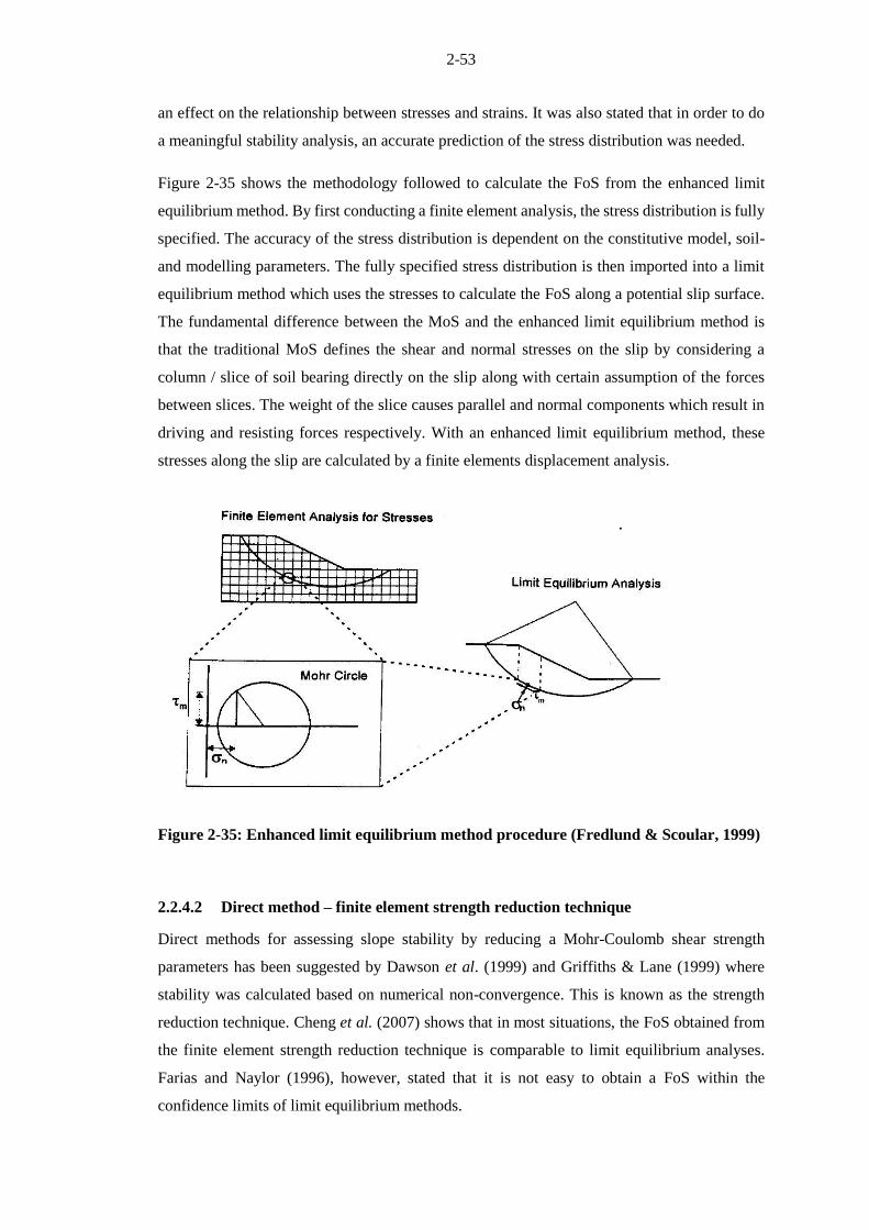
2-53
an effect on the relationship between stresses and strains. It was also stated that in order to do
a meaningful stability analysis, an accurate prediction of the stress distribution was needed.
Figure 2-35 shows the methodology followed to calculate the FoS from the enhanced limit
equilibrium method. By first conducting a finite element analysis, the stress distribution is fully
specified. The accuracy of the stress distribution is dependent on the constitutive model, soil-
and modelling parameters. The fully specified stress distribution is then imported into a limit
equilibrium method which uses the stresses to calculate the FoS along a potential slip surface.
The fundamental difference between the MoS and the enhanced limit equilibrium method is
that the traditional MoS defines the shear and normal stresses on the slip by considering a
column / slice of soil bearing directly on the slip along with certain assumption of the forces
between slices. The weight of the slice causes parallel and normal components which result in
driving and resisting forces respectively. With an enhanced limit equilibrium method, these
stresses along the slip are calculated by a finite elements displacement analysis.
Figure 2-35: Enhanced limit equilibrium method procedure (Fredlund & Scoular, 1999)
2.2.4.2 Direct method – finite element strength reduction technique
Direct methods for assessing slope stability by reducing a Mohr-Coulomb shear strength
parameters has been suggested by Dawson et al. (1999) and Griffiths & Lane (1999) where
stability was calculated based on numerical non-convergence. This is known as the strength
reduction technique. Cheng et al. (2007) shows that in most situations, the FoS obtained from
the finite element strength reduction technique is comparable to limit equilibrium analyses.
Farias and Naylor (1996), however, stated that it is not easy to obtain a FoS within the
confidence limits of limit equilibrium methods.

2-54
The use of finite elements in recent times has been controversial. In the past, catastrophic
failures, notably the Nicoll Highway Collapse in 2004, have been partially attributed to the
misinterpretation of finite element procedures (COI, 2005). Numerous warnings have been
issued cautioning engineers to the appropriate use of finite element analyses in general. Potts
(2003), in his Rankine Lecture, states that the potential for making errors using finite elements
as a geotechnical tool is large. Engineers should be educated in understanding soil mechanics,
the uses and limitations of constitutive models and understanding the assumptions made within
software packages to avoid errors occurring (Potts, 2003). Furthermore, Sloan (2013) and
Krahn (2003) cautions the use of the strength reduction technique as often failure relies on non-
convergence of the numerical solution. Care should be taken that the non-convergence is indeed
a result of genuine collapse and not some other artefact resulting in numerical instability.
Furthermore, Krahn (2003) suggests that a total new method, such as the strength reduction
technique, lacks experience and calibration accustomed to limit equilibrium methods that have
been around for a long time. Sloan (2013) recognises that the potential of finite elements in
solving complex problems is good but the complexities in the method should be well
understood.
Griffiths and Lane (1999) take on a far more positive stance, advocating the use of finite
element modelling in slope stability applications. It is explicitly stated, that the perception of
finite element analysis being complex and misleading is somewhat unwarranted. Furthermore,
readers are reminded that conventional analysis such as method of slices could very well also
be misleading. The amenability of finite elements towards computations of stability of
excavations should therefore be viewed as a relative comparison, as all methods in geotechnical
engineering make dramatic assumptions.
Flow rule / dilation
The issue of analysing a slope stability problem with a non-associated flow rule has been
investigated by Nordal (2008). It has been observed that numerical inaccuracies and oscillations
occur with the FoS making it difficult to define a unique value. Different thoughts are given in
literature around the use of the dilation angle giving rise to a non-associated or associated flow
rule. Generally, it is accepted that the dilation angle for soils under drained conditions is less
that the angle of friction (Bolton, 1986). The consequence of this statement has been
investigated in a numerical context, primarily on slope stability problems, and it has been found
that under many circumstances that the angle of dilation does not have a significant impact on
the FoS. Cheng et al. (2007) finds that under most circumstances the FoS obtained using an
associated flow rule is only slightly larger than using a dilation angle of zero. Tschuchnigg et
al. (2015) documents that the dilation angle has a noticeable impact for steep slopes with high

2-55
friction angles. The differences are however, small and can be attributed to the low level of
kinematic constraint of the problem. However, under complex geometries, such as a problem
with a soft soil band, the flow rule is indeed an issue in the strength reduction technique. The
choice in dilation angle has a significant influence on bearing capacity problems due to
confinement (Griffiths, 1982). The confinement and angle of dilation has not extensively been
investigated for retaining walls.
Cheng et al. (2007) suggests that in the same way that the limit equilibrium MoS suffers from
the choice of interslice forces, the finite element strength reduction technique suffers from the
choice of flow rule which in some cases has an impact on the stability result.
2.2.4.3 SIGMA/W
The GeoStudio suite includes programs for limit equilibrium, seepage, seismic and finite
element deformation computations. SIGMA/W is a program within the GeoStudio suite used
for finite element displacement analysis in geotechnical applications. GeoStudio is part of
GEO-SLOPE International Ltd.
SIGMA/W can be used as the finite element phase of the enhanced limit equilibrium method
calculation. The second part of the calculation was conducted using SLOPE/W, which is a
programme incorporating the method of slices. SLOPE/W is discussed in Section 2.2.3.3.
SIGMA/W is combined with SLOPE/W to calculate stabilities using the enhanced limit
equilibrium method.
This section briefly discusses the various modelling inputs using SIGMA/W Version 2007. For
an in-depth description of how the software works, refer to ‘SIGMA/W 2007 Stress-
Deformation Modeling Guide’.
Model
A plane strain two-dimensional model was used in SIGMA/W representing an infinitely long
wall having the same cross-section. Structural elements can only be modelled in plane strain.
Finite element mesh
The soil continuum is subdivided into finite elements to enable calculation procedures to
commence. The discretisation is called a mesh. The mesh can comprise of many or few
elements, the shape can vary and the number of nodes within each element differ.
SIGMA/W uses a fully automated meshing procedure. An ‘unstructured’ mesh aligns the
discretised mesh elements with geometric or structural objects. SIGMA/W recommends using
a combination of quadrilateral and triangular elements.

2-56
A selection of 3-noded triangular or 4-noded quadrilateral elements can be selected for first
order elements. Higher order elements can be selected such as 6-noded triangular or 8-noded
quadrilateral elements providing second order integration.
SIGMA/W uses a global element size to define the mesh resolution. Geometric points, lines or
regions can be refined/enlarged by defining a ratio of the selected global element size. This is
useful in areas close to structures with large deformation gradients.
Beams
Beam elements can use used as structural bodies which are essentially plates in the out of plane
direction. Beam elements have axial and flexural stiffness properties (Young’s modulus, area,
moment of inertia).
Beam nodes are automatically specified to coincide with the number of nodes on the adjacent
soil element edge. Beams nodes have three degrees of freedom per node (two translational and
one rotation).
Plates are based on Bernoulli beam theory (Owen and Hinton, 1982). Beam elements are linear
elastic materials and cannot take plasticity into account.
Bars
Bar elements can be described as springs that ties two points together in the model. Contrary to
other structural elements (e.g. beams), bars do not divide or create soil elements along its
geometry. Bar elements span across soil elements linking only the end points.
Bars have a constant axial stiffness specified using Young’s modulus and the bar area. Bars are
linear elastic and cannot take plasticity into account.
2.2.4.4 PLAXIS
PLAXIS is a finite element program used for deformation and stability analyses in geotechnical
applications. PLAXIS originates from the Delft University of Technology where it was first
developed in 1987. Over the years a company named PLAXIS b.v. was formed and a host of
finite element programs were developed including, 2D, 3D, deformation, seepage and dynamic
analyses (PLAXIS, 2016).
PLAXIS 2D, Version 2016 (referred to as PLAXIS) was used and is the focus of subsequent
discussions.
This section briefly discusses the various modelling inputs using PLAXIS. For an in-depth
description of how the software works, refer to PLAXIS, 2016, Reference Manual.

2-57
Model
A plane strain model can be used if the cross-section is fairly uniform for a long distance. Figure
2-36 shows a plane strain lateral support geometry with a discretised mesh. For a plane strain
model, the strains in the z-direction are assumed to be zero.
Figure 2-36: Example of plane strain analysis (adapted from PLAXIS, 2016)
Mesh
PLAXIS allows the use of 6- or 15-noded triangular elements to construct the mesh. 15-noded
elements provide a forth order interpolation for displacements and the numerical integration
involves 12 Gauss / Stress points as shown in Figure 2-37. It has been shown that higher order
elements provide good accuracy to finite element calculations (Sloan, 1981; Sloan & Randolph,
1982).
Figure 2-37: Fifteen-noded triangular elements

2-58
PLAXIS allows for an automatic mesh generation procedure. The target average element size,
le, is given by Equation (2.18). The relative element size factor, re, is based on a qualitative
description from very course to very fine as shown in
Table 2-10. PLAXIS recommends initial simulations to be run on a medium mesh resolution
and then the final calculation to be done on a very fine resolution.
𝑙𝑒 = 𝑟𝑒 ∙ 0.06 ∙ √(𝑥𝑚𝑎𝑥 − 𝑥𝑚𝑖𝑛)2 + (𝑦𝑚𝑎𝑥 − 𝑦𝑚𝑖𝑛)
2 (2.18)
Where x and y are the boundary positions.
Table 2-10: Mesh resolution according to qualitative descriptor
Mesh resolution descriptor Relative element size
factor, re
Approximate number of
elements
Very Course 2.00 30 – 70
Coarse 1.33 50 – 200
Medium 1.00 90 – 350
Fine 0.67 250 – 750
Very Fine 0.50 500 – 1250
The mesh size as described applies to the global element size. In areas where high stress
concentrations occur or where large deformation gradients are expected, the mesh should be
refined. PLAXIS automatically refines the mesh around structural elements such as plates,
anchors and embedded beam rows to one quarter of the average element size. The user can
further refine the mesh close to structural elements if required.
Plates
Plate elements are the same as beam elements over a 1m spacing in the z-direction. Plate
elements have axial and flexural stiffness properties (Young’s modulus, area, moment of
inertia). The equivalent plate thickness is calculated for a rectangular beam/plate with 1m
width. Plate nodes have three degrees of freedom per node (two translational and one rotation).
Five noded elements are used which are compatible with the 15-noded triangular soil elements.
Plates are based on Mindlin’s beam theory which considers axial, shear and bending
deformation (Bathe, 1982). Plates can be defined as elastic perfectly-plastic materials to take
plasticity into account. A maximum axial force and moment can be specified to define the

2-59
material yield point. The yield point of a force-moment loading combination is defined by a
linear proportionality as shown in Figure 2-38. Upon yielding, plate elements deform in
extension or rotation without any addition in force / moment. The connection between plates
and other structural elements can be fixed, hinged or free.
Figure 2-38: Maximum/plastic force-moment loading combination (PLAXIS, 2016)
Interfaces
Interface elements can be specified to form the boundary between a structural element (eg.
plate) and the soil continuum. A typical application of an interface is between a sheet pile wall
and the soil. The wall friction and adhesion in many cases is less than the friction angle and
cohesion of the soil and thus an interface factor, Rinter, less than unity, can be specified.
Unless good contact is made between a structural element and the adjacent soil, the shear
strength on the contact could be less than that of the soil. The purpose of interfaces in PLAXIS
is to model this reduction in strength.
The interface friction angle between the structural elements, such as a sheet pile wall, and the
soil will have an impact on the stability. The same can be said for the interaction between the
shotcrete and the soil (also applicable to soil-nails). FHWA (1999) recommends an interface
friction angle of 0.5ϕ' to 1.0ϕ'.
PLAXIS uses an interaction factor, Rinter, to describe the soil-structure interface. The interaction
reduces the shear strength characteristics of the adjacent soil according to Equation (2.19).
𝑅𝑖𝑛𝑡𝑒𝑟 = 𝑐𝑖𝑐𝑠𝑜𝑖𝑙
= tan (𝜙′𝑖)
tan (𝜙′𝑠𝑜𝑖𝑙) (2.19)
Np
Moment, M
Axial Force, N
-Np
Mp-Mp

2-60
Where subscripts ‘i’ and ‘soil’ represent the shear strength characteristics of the interface and
soil elements respectively.
Brinkgreve et al. (2010) suggest interaction factors as shown in Table 2-11. A high interaction
factor implies greater friction between the structural element and the soil thus increasing
stability. PLAXIS (2016) suggest that in the absence of detailed information, a conservative
interaction factor of Rinter = 0.66 should be used. If no cohesion is present, an interaction factor,
Rinter = 0.66, is equivalent to a wall friction angle of 0.8 ϕ'. Using an interface value of unity is
the same as omitting the interface altogether.
Table 2-11: Suggested interaction factors (Brinkgreve et al. 2010)
Interaction materials Rinter
Sand – Steel 0.6 – 0.7
Clay – Steel 0.5
Sand – Concrete 0.8 – 1.0
Clay – Concrete 0.7 – 0.7
Node-to-node anchors
Node-to-node anchors can be described as springs that ties two points together in the model.
Contrary to other structural elements (e.g. plates), node-to-node anchors does not divide or
create soil elements along its geometry. Node-to-node anchors span across soil elements linking
only the end points.
Node-to-node anchors have a constant normal stiffness (i.e. axial). However, the maximum
compressive or tensile forces can be limited to represent failure. Therefore, the material is
modelled as an elastic perfectly-plastic material.
Embedded beam rows
Embedded beam rows can be used to model structural elements such as piles, rock bolts or
ground anchors. Embedded beam rows include axial and flexural stiffness properties,
interaction properties with the surrounding soil and the out of plane spacing of the elements.
The stiffness properties are defined by the geometrical shape and Young’s modulus. The
moment of inertia for a circular shaped element can be specified in terms of the diameter, D, as
shown in Equation (2.20).

2-61
𝐼 =1
64𝜋𝐷4 (2.20)
The interaction between the embedded beam row and the surrounding soil is governed by
limiting the allowable skin friction, Tmax. The skin friction is specified along the length of
embedded beam as a force per length (kN/m). A linearly varying skin resistance between the
top and bottom of the beam can also be specified. Additionally, elements such as piles can also
have an end bearing resistance, Fmax, so that the total resistive force is given by Equation (2.21).
𝑁𝑡𝑜𝑡𝑎𝑙 = 𝐹𝑚𝑎𝑥 + 1
2 𝑒𝑛𝑔𝑡ℎ ∙ (𝑇𝑡𝑜𝑝,𝑚𝑎𝑥 + 𝑇𝑏𝑜𝑡,𝑚𝑎𝑥) (2.21)
Previous modelling
Fan & Luo (2008) and Shiu & Chang (2006) used PLAXIS to model soil-nailed structures using
Plates and Interface elements. Interface elements allow for movement between two materials
such as the plate and soil. However, the strength of the interface element is specified as some
factor of the adjacent soil which is a function of effective stress and hence the depth. Heymann
(1992) has shown that the pull-out resistance of soil-nails installed in over-consolidated soils
such as residual andesite and granite in South Africa is not a function of the effective stress and
is independent of depth.
The combination of node-to-node anchors and embedded pile rows, for the free- and fixed-
lengths of anchors respectively, has been successfully demonstrated by Gens (2012) using
PLAXIS.
2.2.5 Other methods
2.2.5.1 Mobilised Strength Design (MSD)
In practice, there is a distinction between collapse calculations for stability and calculations to
predict and limit movements of retaining structures. Plasticity theory (and consequently derived
limit equilibrium analyses) is often used to quantify the stability of a design. Elasticity theory
has been used to predict displacements. However, some ‘equivalent’ modulus has to be used to
predict acceptable movements (Osman & Bolton, 2004).
Generally, codes of practice predict collapse loads with various methods and global or partial
factors are applied to ensure that stresses under working conditions are sufficiently far away
from their ultimate values. The margin between working and ultimate stresses are generally
sufficient to limit unacceptable movements but are never calculated. Codes of practice do not

2-62
deal in depth with serviceability issues which can be as, if not more, critical than stability
(Simpson & Driscoll, 1998).
From the shortcomings of current design practice, Bolton et al. (1990a, 1990b) proposed an
approach which will enable designers to predict collapse and movements in a single calculation:
Mobilised Strength Design (MSD). Osman and Bolton (2004) has demonstrated the method for
a simple case of a cantilevered retaining wall.
The MSD approach requires only soil stress-strain data to be derived from a representative
undisturbed soil sample. The representative data from the soil sample is the empirical solution
to governing the stress-strain relationship of the specific soil.
The method, as shown in Figure 2-39, is described below:
1. A plastic deformation mechanism is assumed with compatible strains as shown in
Figure 2-40. The mechanism can be derived from field data, centrifuge testing and/or
finite element modelling. With this mechanism, solutions are derived relating strains
to incremental displacements. Strains within the soil and the retaining structure are both
considered.
2. The solution is derived on the basis of the principle of virtual work where the external
work is equated to the internal stored energy. The external work is simply the product
of the weight of soil being displaced and the incremental displacement. The internal
work done by the soil resisting deformation is calculated from a stress-strain curve as
shown in Figure 2-41. From the strain that is derived given an incremental
displacement, a corresponding stress is observed from the stress-strain data. The
internal work is calculated from this mobilised shear strength.
3. Similarly, the energy stored within the deformed structure (eg. embedded retained wall)
is calculated for an incremental displacement.
4. An iterative procedure is carried out by varying the incremental deformation until the
external work equates to the internal work.
The MSD method has been demonstrated for braced excavations in clay (Osman & Bolton
2005, Osman & Bolton 2006). The method is still to be developed for drained conditions.

2-63
Figure 2-39: Principle calculation procedure (Bjureland, 2013)

2-64
Figure 2-40: Displacement field for braced excavation (Osman & Bolton, 2006)
Figure 2-41: Stress-strain response of Norwegian quick clay (Bjerrum & Landva,
1966)

2-65
2.3 FACTOR OF SAFETY
The principle aim of the design of lateral support is to ensure stability and limit movements to
an acceptable amount (Atkinson, 1993; SAICE, 1989). The intention of this study is to compare
the stability outputs of different methods of analysis for soil-nails and anchors. Stability can be
defined as equilibrium of activating and resisting forces (or moments). As a designer, a certain
margin of safety against instability should be provided where instability is the failure of the
system. To quantify this margin of safety, Factor of Safety (FoS) is a commonly used approach.
It is important to note that the FoS is a indicative measure of stability but not an absolute.
A FoS of 1.0 means that the slope is on the verge of failure as resisting forces is exactly equal
to driving forces. A FoS of 2.0 would broadly mean that there is twice as much force resisting
as driving. FoS is a somewhat arbitrary and ambiguous quantification of stability as different
definitions exist to what is considered as resisting and driving forces. For example, it is argued,
that weight of the soil is one entity and the net effect thereof should be considered not the
individual components. Reinforcement is often considered as a negative driving force.
Furthermore, FoS is non-linear with respect to probability of failure, which can be misleading
to inexperienced designers (SAICE, 1989).
By way of an example, suppose a lateral support system exists with a FoS of 1.0 which means
that the driving forces is the same as the resisting forces. The engineer specifies ground anchors
equivalent to 50% of resisting forces. The FoS will then be,
FoS = Resisting
Driving= x + 0.5x
x= 1.5 (2.22)
If the anchors are considered as a negative driving force (SAICE, 1989), the FoS will be,
FoS = x
x − 0.5x= 2.0 (2.23)
The lateral support is exactly the same and hence the stability is identical, however, the FoS
differs. Therefore, the definition of activating forces and resisting forces is critical to the
outcome of FoS. Different codes adopt different definitions of FoS (Fang, 1991; SAICE, 1989;
Sheahan & Ho, 2003).
2.3.1 Definitions
To explain the different definitions of FoS, consider Figure 2-42 which shows the forces acting
on a soil-nail/anchored system analysed with a single wedge failure mechanism. Two
contributing factors, the tension from the reinforcement, T, and the weight of the soil, W, exist
and each of these have a component parallel (subscript //) and perpendicular (subscript ┴) to the
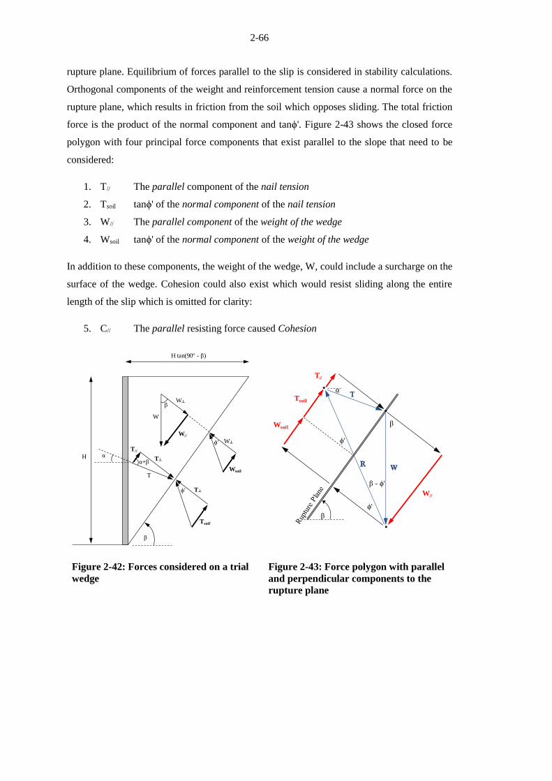
2-66
rupture plane. Equilibrium of forces parallel to the slip is considered in stability calculations.
Orthogonal components of the weight and reinforcement tension cause a normal force on the
rupture plane, which results in friction from the soil which opposes sliding. The total friction
force is the product of the normal component and tanϕ'. Figure 2-43 shows the closed force
polygon with four principal force components that exist parallel to the slope that need to be
considered:
1. T// The parallel component of the nail tension
2. Tsoil tanϕ' of the normal component of the nail tension
3. W// The parallel component of the weight of the wedge
4. Wsoil tanϕ' of the normal component of the weight of the wedge
In addition to these components, the weight of the wedge, W, could include a surcharge on the
surface of the wedge. Cohesion could also exist which would resist sliding along the entire
length of the slip which is omitted for clarity:
5. C// The parallel resisting force caused Cohesion
Figure 2-42: Forces considered on a trial
wedge
Figure 2-43: Force polygon with parallel
and perpendicular components to the
rupture plane
W
W┴
W//
W┴ϕ'
ϕ'
Wsoil
Tsoil
T
β
α+β
T//
β
T┴
T┴
H
H tan(90° - β)
α
W//
Tsoil
Wsoil
β
ϕ'
ϕ'
T//
α
β
β - ϕ'

2-67
An intuitive way of defining the FoS would be to regard all forces acting up the slope as
resisting and forces down the slope as driving. Hence,
FoS = Resisting
Driving= C|| + T||+ Tsoil +Wsoil
W||
(2.24)
The second definition considers the parallel component of the nail tension, T//, as a negative
driving force as shown in Equation (2.25). This is best understood by recognising that the FoS
exists to account for variability in the system. It is well known variability of soil parameters far
outweighs that of the steel reinforcement which is well defined and manufactured under
controlled conditions (Harr, 1977). It would therefore make sense to arrange the FoS equation
in such a way to reduce the forces relying on the soil parameters as shown in Equation (2.26).
FoS required ≤ FoS = C||+ Tsoil +Wsoil
W|| − T|| (2.25)
W|| − T|| ≤ C||+ Tsoil +Wsoil
FoS required (2.26)
The implication of Equation (2.26) is that the shear strength components are being reduced by
the FoS. This is synonymous to the Strength Reduction Factor (SRF), which is defined as the
amount that c' and tanϕ' needs to be simultaneously reduced for failure to occur. Failure occurs
when FoS is below unity as shown in Equation (2.27).
1.0 ≤ C||+ Tsoil +Wsoil
SRF (W|| − T|| ) (2.27)
The definition of FoS used in Equation (2.24) is used by American literature such as Sheahan
& Ho (2003), FHWA (2003) and Babu & Singh (2011).
FoS =
cHsinβ
+Wcosβtanϕ′ + [Ticos(β + α) + Ti sin(β + α) tanϕ′]ni=
Wsinβ
American
definition
FoS = C|| +Wsoil+T|| + Tsoil
W||
(2.28)

2-68
The definition of FoS in Equation (2.25) is used by British/South African literature such as BS
8081(1989) and SAICE (1989).
FoS =
cHsinβ
+Wcosβtanϕ′ + [Tisin(β + α) tanϕ]ni=
Wsinβ − [Ticos(β + α)]ni=
British / South
African definition
FoS = C|| +Wsoil+ Tsoil
W|| − T||
(2.29)
Where,
H is the height of the retained face
β is the angle of the trial failure wedge
α is the angle of installation of the reinforcement
Ti is the maximum reinforcement resistance of ith soil-nail/anchor
ϕ' is the angle of friction of the soil
c is the soil cohesion
Both of these FoS consider equilibrium of the slip surface and the reinforcement in one
equation. The pull-out resistance of soil-nails is often investigated by considering the nail
capacity. The “German Method”, pioneered by the early work of Stocker et al. (1979) and
Gässler and Gudehus (1981), uses a bilinear double wedge failure to define the FoS as the ratio
available nail capacity to the required soil-nail capacity to main equilibrium. The “Davis
Method” (Shen et al. 1981) specifies the FoS in terms of the soil shear strength. Juran and Elias
(1987) advocate placing the FoS on the reinforcement capacity. SAICE (1989), in addition to
evaluating the overall stability as stated earlier, recommend that the FoS also be checked against
soil-nail capacity using a wedge method proposed by Gässler (1988) as shown in Equation
(2.30).
FoS = Tprovided
Trequired (2.30)
Where Trequired is computed using a limit equilibrium wedge with the FoS set to 1.0 against soil
resistance. By setting the FoS = 1.0, either the American [Eq (2.28)] or the British/South
African [Eq (2.29)] equations can be rearranged to obtain,
1.0 =
cHsinβ
+Wcosβtanϕ′ + [Ticos(β + α) + Ti sin(β + α) tanϕ′]ni=
Wsinβ
(2.31)

2-69
Where Ti is the tension force required. Rearrangement gives,
Trequired = Wsinβ −
cHsinβ
− Wcosβtanϕ′
cos(β + α) + sin(β + α) tanϕ′
(2.32)
Using the simplified nomenclature given earlier,
Trequired = 𝑊|| − 𝐶|| − 𝑊𝑠𝑜𝑖𝑙
cos(β + α) + sin(β + α) tanϕ′ (2.33)
Equation (2.30) can now be expanded by substituting Equation (2.33),
FoS = Tprovided
W|| − C|| − Wsoil
cos(β + α) + sin(β + α) tanϕ′
FoS = Tprovided[cos(β + α) + sin(β + α) tanϕ′]
W|| − C|| − Wsoil
The German
Definition FoS =
T|| + TsoilW|| − C|| − Wsoil
(2.34)
As shown in Equation (2.34), the German Method can also be rewritten in the same form as the
other definitions of FoS. The German Method factors the nail / anchor capacity to obtain
suitable stability requirements.
2.3.2 FoS as a design requirement
Codes or standards of practice lay down the minimum requirements for the end product which,
in this case, will ensure safe and practicable design. Importantly, codes and standards provide
a statement of what is deemed to be reasonable and acceptable practice (Day, 2013).
In South Africa, a code of practice to guide engineering practitioners on the subject of lateral
support was first published in 1972. The same code was revised and updated over a period of
five years by the geotechnical division of SAICE and Code of Practice – 1989 was published
(SAICE, 1989).
A code of practice is commonly used in South Africa as a design aid and a document which
proves reasonable measures by the designer. All standards are considered voluntary unless
referenced by legislation or stipulated in the contractual agreement. One such occurrence in
South African legislation is Act 103 of 1977: National Building Regulations and Building
Standards Act. Figure 2-44 shows an extract out of SANS 10400-G which is the application of

2-70
the National Building Regulations for excavations. As shown, SANS 10400-G makes explicit
reference to the SAICE Code of Practice. Therefore, in the design of lateral support, deviation
from the code of practice could result in legal consequences.
The SAICE Code of Practice and other codes makes numerous references to the FoS as a
measure of adequate stability. The concept of FoS is well established in geotechnical practice
(Sloan, 2013) and lateral support codes all around the world still use the FoS as a measure of
stability. Therefore, the importance of the accurate determination of FoS remains paramount to
a lateral support design.
Figure 2-44: Extract from SANS 10400-G
The following summary is presented on significant aspects related to the factor of safety:
There is no unique definition for FoS with regard to soil-nails and anchors
Different definitions exist due to various authors attributing the variability in a design
to different components.
o Some American literature use an approach defining the FoS in terms of forces
resisting failure opposing the direction of movement (i.e. forces up the failure
plane) and forces driving failure (i.e. forces down the failure plane). The FoS
is defined as the ratio of resisting over driving forces.
o Some British and South African literature have modified the equation in order
to attribute the FoS to the soil shear strength parameters. This is synonymous
to using a strength reduction factor.
4 Requirements
4.1 General
The functional regulation G1(1) contained in part G of the National Building Regulations
(see annex A) shall be deemed to be satisfied where the excavation relating to a building
is the subject of a rational design or a rational assessment (or both) prepared by a
competent person (civil engineering) or competent person (engineering geology)…
NOTE 3: The South African Institution of Civil Engineering’s (Geotechnical Division)
Code of practice for lateral support in surface excavations provides practical guidance to
enable a competent person (civil engineering) or competent person (engineering geology)
to comply with the requirements of 4.1(b).
2-71
o For soil-nails specifically, some authors have stipulated a FoS in terms of the
soil-nail capacity (pull-out and/or yield).
If the FoS is set to 1.0, Equations (2.28), (2.29) and (2.34) are the same. In other words,
if a partial factor method is used, attributing variability to each component a unique
FoS could be specified.
Partial safety factors were not applied in this work and is beyond the scope. For limit
equilibrium methods, the calculated FoS was compared to the strength reduction factor
calculated from the finite element strength reduction technique.
The FoS remains a critical quantity in defining adequate geotechnical design of lateral
support systems. Codes of practice make numerous reference to the Factor of Safety
and gives guidance to the required values. Adherence to code of practice is important
in terms of legal and sound engineering requirements.

2-72
2.4 SUMMARY
The use of soil-nails is a fairly new method of soil reinforcement, rapidly expanding since the
1980s. Despite considerable work since then, the design of soil-nail support is based upon
simplified and conservative models. A general consensus is reached (Jewell & Pedley, 1992;
Pedley et al.; Bridle & Davis, 1997) that soil-nails can adequately be specified as tensile
members under normal angles of installation. The pull-out resistance in many soils can be
calculated as a function of effective stress. However, Heymann (1992) has shown that in South
African residual soils, the pull-out resistance is independent of depth.
Anchored lateral support systems were implemented since the 1930s. The design of anchored
lateral support systems is based on an acceptable working load according to the appropriate
code of practice. Working loads, typically in the region of 150kN/strand, are obtained from a
factored down characteristic ultimate load. Anchored fixed-lengths are often pressure grouted
in order to obtain sufficient bond resistance. Soldier piles are often incorporated in anchored
systems. Solider piles could aid stability, creating passive resistance which can be analysed
with simple methods such as Broms (1965) or Wang-Reese (1986).
Tschuchnigg et al. (2015) and other authors confirmed that limit equilibrium methods are
widely and routinely used in practice for the analysis of slope stability. Being routed in slope
stability, lateral support problems are often also addressed using the same limit equilibrium
methods. In several codes, limit equilibrium methods, such as the trial wedge or method of
slices, are recommended to evaluate the stability of a retaining structures to an acceptable
defined Factor of Safety. For decades, these limit equilibrium methods have been used
successful in providing an acceptable margin of safety against failure (movements, which can
be significantly more complex, is not considered).
Advances in other methods that analyse stability have occurred since the acceptance of limit
equilibrium methods. In recent years, the ideas of finite elements and plasticity have been
combined. Finite element limit analysis provides rigorous upper and lower bounds and the error
of a solution can be computed (Tschuchnigg et al. 2015; Sloan, 2013). Mobilised Strength
Design (Osman & Bolton, 2004) incorporates a stability and deformation analysis in a single
calculation. Finite element limit analysis and mobilised strength design are amongst the
forerunners of new methods of analysis.
Since Griffiths and Lane (1999) popularised the idea of using a strength reduction factor in
finite element displacement analyses, an increase in the use thereof to calculate the FoS has
been observed in industry (Tschuchnigg et al. 2015). Potts (2003) cautions users to the
misinterpretation and limitations of finite element results. Cheng et al. (2007) has found that
2-73
limit equilibrium methods can compare with finite element strength reduction methods.
However, Tschuchnigg et al. (2015) agrees, that non-associated flow has noticeable
implications on stability calculations. For the strength reduction technique, the effects of
dilation, tolerance, soil moduli and boundary effects are small but noticeable.
Krahn (2003) suggests using a combined finite element and limit equilibrium approach to
calculate the Factor of Safety. A finite element analysis is used to obtain the stress distribution
throughout the soil continuum. A limit equilibrium analysis is then used to evaluate the Factor
of Safety based on the finite element calculated stresses.
Other studies have been conducted comparing the use of the finite element strength reduction
technique to other methods. However, most of these studies consider slope problems. Few
studies have been conducted for lateral support systems. Cheng et al. (2007) concludes that the
finite element strength reduction technique cannot be seen as superior to the method of slices
and that each method must be viewed on their unique advantages and disadvantages. Cheng et
al. suggests that the method of slices should be used as a cross reference tool for finite element
methods.
The concept of Factor of Safety is well established in geotechnical engineering (Sloan, 2013).
However, there is no unique definition for it. Within lateral support, different codes have
different definitions of the Factor of Safety (FHWA, 1999; SAICE, 1989). The Factor of Safety,
albeit somewhat arbitrary, remains a critical number in the determination of stability in
geotechnical problems. Codes of practice make numerous reference to Factor of Safety and
gives guidance to the required values. Adherence to code of practice is important in terms of
legal requirements and good engineering practice.
A study is necessary to evaluate the differences between different stability calculations in terms
of Factor of Safety, comparing the well-established, simplistic, limit equilibrium methods and
newer, more complex, finite element methods for soil-nails and anchors.


CHAPTER 3 ANALYSIS PROCEDURES
In this chapter, the methodology used to compare different methods of analysis and their
implications on stability calculations is described. The analysis methods are applied to different
methods of support.
3.1 INTRODUCTION
Four methods of analysis were applied to analyse various geometries. The geometries were a
uniform slope, soil-nail supported face and a face supported by anchors. The design and
assumptions regarding the three geometries analysed is firstly discussed, followed by the four
methods of analysis.
The three different geometries analysed are listed below and discussed in more detailed in
Section 3.2:
1. Uniform slope. A 1:2 (vertical to horizontal), homogenous slope was analysed. The
purpose the geometry is to view the differences in methods of analysis with the simplest
case without any addition in reinforcing.
2. Soil-nailed excavation. An 8.5m deep excavation support by soil-nails was analysed
with various methods.
3. Anchored excavation. An 17m deep excavation supported by anchors (tie-backs) was
analysed with various methods.
The four methods of analysis considered are listed below and discussed in more detailed in
Section 3.3:
1. Limit Equilibrium – Single Trial Wedge Failure (Wedge Method). This method is
easily carried out by hand calculation and was programmed in a spreadsheet using the
trial wedge method (Sheahan & Ho 2003).
2. Limit Equilibrium – Method of Slices (MoS). This is a well-established method
adopted in geotechnical practice, generally for slope stability analysis. The software
package GeoStudio SLOPE/W was used to model circular slip surfaces using the
Morgenstern-Price (1965) method.

3-2
3. Enhanced Limit Equilibrium (ELE Method). This method uses a finite element
analysis to compute the stresses throughout the soil continuum using the SIGMA/W
program. A slip circle analysis is then applied using SLOPE/W as with the Method of
Slices. The program can search for critical slip surfaces. The primary difference
between the ELE Method and MoS, is that the stresses are calculated using a finite
element model versus simply the weight of a slice and assumed inter-slice forces
(Naylor, 1982).
4. Finite Element Strength Reduction Factor (FE (SRF) Method). A finite element
analysis with the strength reduction technique (Zienkiewicz et al. 1975; Griffiths &
Lane, 1999) was used to compute the Strength Reduction Factor (SRF) for the various
geometries. In this method, the shear strength parameters, tanϕ' and c', are reduced by
escalating the SRF until failure occurs or until deformations become large. The degree
by which the shear strength parameters can be reduced before failure occurs is an
indicator of stability. The software package PLAXIS was used which incorporates a
built-in SRF procedure (Brinkgreve & Bakker, 1991; PLAXIS, 2016).
3.2 GEOMETRIES ANALYSED
In order to investigate the influence of the method of analysis on the design of lateral support
for excavations, three different geometries were analysed. The three geometries that were
analysed are:
1. Uniform slope
2. Soil-nailed excavation
3. Anchored excavation
All three cases were evaluated for stability with the limit equilibrium (Wedge and MoS),
Enhanced Limit Equilibrium and the Finite Element (Strength Reduction Factor) Methods. This
section describes the geometries, parameters and assumptions made with regard to each of these
three cases.
3.2.1 Material parameters
All three geometries were analysed using a standard set of material parameters. The parameters
were obtained from geotechnical investigations done for the soil-nailed and anchored lateral
support systems. Both lateral support systems were excavated within residual granite.
The material parameters used for this study are summarised in Table 3-1. A simplifying
assumption was made that the material is uniform, homogenous and isotropic throughout the

3-3
geometry profile. The friction angle, cohesion and unit weight parameters was selected for a
slightly cemented dense granular soil. The angle of dilation was taken as ½ ϕ' which is a typical
value when applying the stress-dilatancy expressions by Bolton (1986). Young’s modulus was
taken as 90MPa representing a dense material (Jennings et al. 1973; Bowles, 1996). Poisson’s
ratio was taken as 0.3 as estimated by Bowles (1996). An elastic-plastic (Mohr-Coulomb) soil
model applied using the parameters as described.
Table 3-1: Residual granite assumed parameters
Parameter Units Value
Friction Angle, ϕ' ° 36
Cohesion, c' kPa 3
Unit weight, γ kN/m3 19
Poisson’s ratio, v' 0.3
Stiffness, E’ MPa 90
Angle of dilation, ψ' ° 18
Soil model Elastic-Plastic (Mohr-
Coulomb yield criterion)
3.2.2 Uniform slope
The first case is that of a 15m high, uniform soil slope with a 1:2 (26.6°) vertical to horizontal
gradient as shown in Figure 3-1. Residual granite, with properties discussed in the previous
section, was used to model the slope. The differences in FoS calculated by the four methods of
analysis were investigated. Since most of the analysis methods for soil-nail and anchor systems
are rooted in slope stability methods, it is worth evaluating the differences between the methods
without the interference of reinforcement and its associated complex soil-structure interactions.
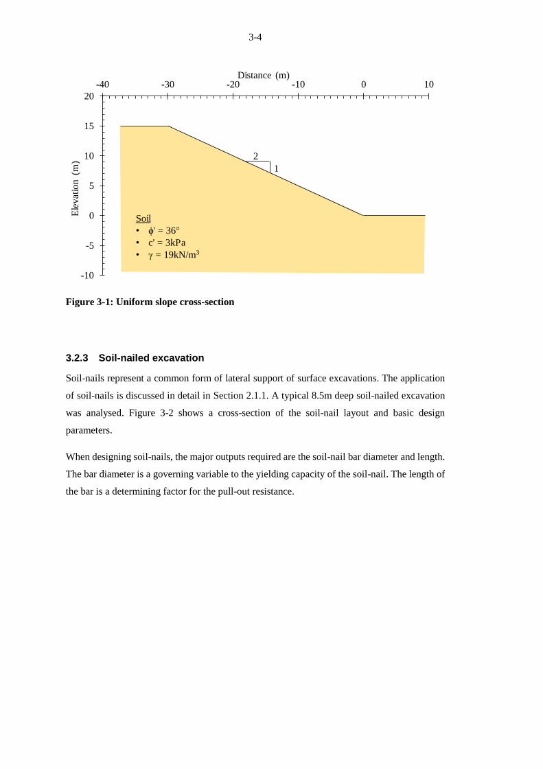
3-4
Figure 3-1: Uniform slope cross-section
3.2.3 Soil-nailed excavation
Soil-nails represent a common form of lateral support of surface excavations. The application
of soil-nails is discussed in detail in Section 2.1.1. A typical 8.5m deep soil-nailed excavation
was analysed. Figure 3-2 shows a cross-section of the soil-nail layout and basic design
parameters.
When designing soil-nails, the major outputs required are the soil-nail bar diameter and length.
The bar diameter is a governing variable to the yielding capacity of the soil-nail. The length of
the bar is a determining factor for the pull-out resistance.
-10
-5
0
5
10
15
20
-40 -30 -20 -10 0 10E
lev
atio
n (
m)
Distance (m)
2
1
Soil
• ϕ' = 36°
• c' = 3kPa
• γ = 19kN/m3

3-5
Figure 3-2: Soil-nailed excavation design
The soil-nail pull-out force is a function of the allowable soil-grout interface shear stress,
drilling diameter and length of soil-nail behind the slip surface. The allowable soil-grout
interface stress was taken as 110kPa. This is a conservative value estimated from 4ϕ', which is
appropriate for residual granites as discussed in Section 2.1.1.5. Considering a drilling diameter
of 102mm (4inch), this will result in a unit pull-out resistance of 35kN/m along the soil-nail
length. The soil-nail bar with a yield stress of 500MPa according to BS 4449:2005 standards
was assumed. A 100mm thick shotcrete face is assumed to adequately transfer the soil load to
the reinforcing (FHWA, 2003).
The bar diameter and soil-nail length was determined using a limit equilibrium wedge analysis
with a target FoS of at least 1.5. Five rows of 6m-long nails of 20mm-diameter were used to
stabilise the excavation resulting in a minimum FoS = 1.58. The critical failure plane was
located extending at 41° above the horizontal from the excavation toe. The design and
reinforcing parameters are summarised in Table 3-2.
Stability analyses were carried out using design parameters. The model, material and design
parameters were then individually varied in order to assess the impact on the FoS for the
various method of analysis. Initially all analyses were carried out using a single excavation
-2
0
2
4
6
8
10
-4 -2 0 2 4 6 8 10 12
Ele
vat
ion (
m)
Distance (m)
100mm shotcrete
10°
8.5m
7.0m
5.5m
4.0m
2.5m
1.0m
0m
Soil-nail bars:
• 6m length
• 20mm diameter
• Sv = Sh = 1.5m
Soil
• ϕ' = 36°
• c' = 3kPa
• γ = 19kN/m3

3-6
stage. This was compared to modelling a more realistic sequential excavation of 1.5 – 2m
excavation stages. Table 3-3 summarises the ranges of the variables that were investigated in
the parametric study.
Table 3-2: Soil-nailed excavation - design parameters
Parameter Units Value
Lateral support design
Material Residual granite
Height / depth m 8.5
Reinforcement provided 5 rows of 6m-length,
20mm-diameter nails
Installation angle below horizontal (ICE, 2012) ° 10
Soil-nail vertical spacing (rows) m 1.5
Soil-nail horizontal spacing (out of plane) m 1.5
Soil-nail bar
Yield stress (BS 4449, 2005) MPa 500
Bar capacity kN 138
Single nail, area mm2 314
Single nail, area at 1.5m spacing mm2/m 209
Steel modulus, E GPa 200
Grouted bar
Grout diameter (4inch drill bit) mm 102
Soil-grout interface resistance (Heymann,
1992) kPa 110
Pull-out capacity kN/m 35
Shotcrete
Thickness (FHWA, 2003) mm 100
Concrete modulus, E (BS8110-2:1985) GPa 25
Moment of inertia per m width m4/m 8.33E-04

3-7
Table 3-3: Soil-nailed excavation – parametric study range
Parameters Units Range 8.5m Soil-
nail default Minimum Maximum
Material properties
Friction angle, φ' ° 20 40 36
Cohesion, c' kPa 0 10 3
Unit weight, γ kN/m3 16 21 19
Young's modulus, E’ MPa 50 500 90
Poisson, v' 0.2 0.49 0.3
In-situ stress, K0 0.43 1 0.43
Design parameters
Soil-nail length m 5 8 6
Soil-nail diameter mm 16 32 20
Surcharge kPa 0 15 0
Stage construction
modelling
Single
Excavation
Excavation
and
installation
Phases
Single
Excavation
3.2.4 Anchored excavation
In general, anchors are stronger and are capable of restraining higher loads than soil-nails.
Anchors are also better at controlling movements due to it being an active system. Anchors are
discussed in detail in Section 2.1.2. Therefore, a 17m deep excavation was designed using

3-8
anchors.
Figure 3-3 shows a cross-section of the anchored excavation design layout and basic
parameters.
When designing anchors, the major outputs required are the anchor capacity and geometry. The
geometry is specified in terms of free- and fixed-lengths. The post-tensioned force to which
anchors are stressed is referred to as the anchor’s working-load. Anchors typically have
additional capacity in excess of the working load that is used to provide for proof testing, lock-
off losses, creep and a material safety factor.
-4
-2
0
2
4
6
8
10
12
14
16
18
-10 -5 0 5 10 15 20 25 30
Ele
vat
ion (
m)
Distance (m)
15.5m
13.3m
11.1m
8.9m
6.7m
4.5m
2.2m
150mm shotcreteAnchors Spacing
• Sv ≈ 2.2m
• Sh = 2.5m
3 x
300kN
2 x
450kN
2 x
600kN
10°
Soil
• ϕ' = 36°
• c' = 3kPa
• γ = 19kN/m3

3-9
Figure 3-3: Anchored excavation design
Working load
Using a limit equilibrium wedge analysis, based on a target FoS of 1.5, a total anchor force of
1193kN is required per metre out of plane. At a horizontal spacing of 2.5m, a force of 2983kN
per ‘column’ of anchors is required. To meet this requirement, 3 rows of 300kN anchors was
used at the top, followed by 2 rows of 450kN anchors and finally 2 rows of 600kN anchors at
the bottom. This equates to a total anchor force of 3000kN per vertical ‘column’ of anchors.
The vertical spacing between anchors is approximately 2.2m to support the 17m excavation.
Free- and fixed-lengths
In addition to the working load, the design requires the length of the anchors to be specified.
The pressure grouted fixed-length should be sufficiently long to withstand the maximum load
on the anchor. Pressure grouting significantly increases the pull-out resistance of the fixed-
length and can resist much larger loads than that of a passive system such as soil-nails as
discussed in Section 2.1.2.4. The adequacy of the fixed-length is typically tested in the field by
the means of a proof load test according to SAICE (1989). A standard fixed-length of 6m is
assumed to adequately resist the anchor loads and was used in the design.
-4
-2
0
2
4
6
8
10
12
14
16
18
-10 -5 0 5 10 15 20 25 30
Ele
vat
ion (
m)
Distance (m)
15.5m
13.3m
11.1m
8.9m
6.7m
4.5m
2.2m
150mm shotcreteAnchors Spacing
• Sv ≈ 2.2m
• Sh = 2.5m
3 x
300kN
2 x
450kN
2 x
600kN
10°
Soil
• ϕ' = 36°
• c' = 3kPa
• γ = 19kN/m3

3-10
In combination with the 6m fixed-length, an adequate free-length has to be specified which can
be a challenge. Consider Figure 3-4 showing a cross-section of an anchored excavation with
three possible slip surfaces:
A. A slip surface occurring through the free-length. In evaluating the FoS, the slip should
have the highest driving force but will also have the full benefit from the resistance of
the anchor. This approach is recommended by Cheney (1984).
B. A slip surface occurring behind the anchor will, generally, have a smaller driving force
but no anchor resistance. This check is recommended by Fang (1991).
C. A slip surface occurring through the fixed-length could will only mobilise part of the
full pull-out resistance force.
Rules of thumb, based on experience are given by several codes, to the length of anchors.
However, due to the high variability in pull-out resistance, analytical procedures remain
somewhat vague. To ensure sufficient free-lengths, SAICE (1989) illustrate that the FoS should
be checked along the front of the anchor grouted length, which is conservative. Kranz (1953)
and Broms (1968) have developed procedures to calculate the FoS with the slip surface passing
through the anchor midpoint. No matter which methodology is used, given the nature of
automatic trial slip searches, it remains difficult to align common anchor points with a single
slip surface. An ‘average point’ could be used, but the judgement of this is becomes subjective.
Furthermore, for a finite element strength reduction technique, only the critical surface can be
viewed.
In order to avoid the idiosyncrasies of the abovementioned methods, the approach of FHWA
(1999) was followed. For a slip surface passing through the fixed-length (i.e. Figure 3-4, slip
surface C.), the pull-out resistance can be taken proportionally to the length of bond behind the
failure surface e.g. ½ the pull-out resistance can be taken for a slip surface passing through the
middle of the fixed-length. The total pull-out resistance of the fixed-length was specified as the
yield capacity of the anchor. This is a valid assumption as the pull-out resistance is tested close
to the yield capacity through proof testing. Slip surfaces occurring across the fixed-length could
potentially result in a pull-out failure mechanism of the individual anchor. Slip surfaces
occurring across the free-length will result in yielding failure.
Seven-wire, 15.2mm diameter steel strands were used according to ASTM A416 standards. An
acceptable working load of 150kN per strand was used (SAICE, 1989; Parry-Davies, 2010). A
shotcrete facing of 150mm thick was assumed. The design and reinforcement properties are
summarised in Table 3-4.

3-11
Stability analyses were carried out using design parameters. The model, material and design
parameters were then individually varied in order to assess the impact on the FoS for the various
methods of analysis. Contrary to soil-nails, the anchored excavation was modelling using stage
construction excavation and installation phases. The influence of embedded soldier piles was
also investigated. A summary of the ranges of the parameters that were investigated is shown
in Table 3-5.
Figure 3-4: Possible slip surfaces for anchors
Slip C through
anchor fixed-length
Slip A through
anchor free-length
Slip B behind
anchor
Free-length Fixed-length

3-12
Table 3-4: Anchored excavation - design parameters
Parameter Units Value
Lateral support design
Material Residual granite
Height / depth m 17
Reinforcement provided 3 x 300kN & 2 x 450kN &
2 x 600kN
Total anchor force kN 3000
Installation angle ° 10
Anchor vertical spacing (rows) m ~2.2
Anchor horizontal Spacing (out of plane) m 2.5
Anchor tendons
Single strand ultimate strength (ASTM A416) kN 261
Single strand yield strength (ASTM A416) kN 235
Single strand working load (SAICE, 1989;
Parry-Davies, 2010) kN 150
Single strand working load at 2.5m spacing kN/m 60
Single strand area (ASTM A416) mm2 140
Single strand area at 2.5m spacing mm2/m 56
Reinforcement modulus, E GPa 200
Bonded length
Length m 6
Total pull-out resistance (per strand) kN 235
Unit pull-out resistance (per strand) kN/m 39
Shotcrete
Thickness (FHWA, 1999) mm 150
Concrete modulus, E (BS8110-2:1985) GPa 25
Moment of inertia per m width (bh3/12) m4/m 2.81E-04
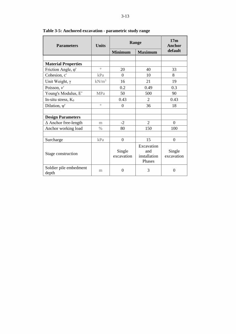
3-13
Table 3-5: Anchored excavation - parametric study range
Parameters Units Range 17m
Anchor
default Minimum Maximum
Material Properties
Friction Angle, φ' ° 20 40 33
Cohesion, c' kPa 0 10 8
Unit Weight, γ kN/m3 16 21 19
Poisson, v' 0.2 0.49 0.3
Young's Modulus, E’ MPa 50 500 90
In-situ stress, K0 0.43 2 0.43
Dilation, ψ' ° 0 36 18
Design Parameters
Δ Anchor free-length m -2 2 0
Anchor working load % 80 150 100
Surcharge kPa 0 15 0
Stage construction Single
excavation
Excavation
and
installation
Phases
Single
excavation
Soldier pile embedment
depth m 0 3 0

3-14
3.3 METHODS OF ANALYSIS CONSIDERED
Four different methods were used to analyse the stability of the geometries discussed. The
procedure followed for the various methods of analysis are discussed in this section.
3.3.1 Wedge Method
The first method used was a planar wedge analysis. This was programmed in Microsoft Excel
based on the Sheahan & Ho (2003) trial wedge method as discussed in Section 2.2.3.1. The
failure wedge is assumed to be a straight line and the exit point is fixed at the toe of the wall.
The entry point (or the angle of slip surface) is then varied in order to obtain the minimum FoS.
The soil shear strength was based on the Mohr-Coulomb failure envelope. The FoS considered
force equilibrium in the direction of the slip surface.
The FoS formulation for both soil-nails and anchors was based on Equation (2.25) which
emphasises the variability in the soil shear strength parameters as discussed in Section 2.3. Only
under this formulation is the FoS from the limit equilibrium wedge method equivalent to the
definition of the FoS for the finite element strength reduction method as discussed in
Section 3.3.4.
Modelling of soil-nails and anchors
The properties of soil-nails and anchors that were modelled are described in Section 3.2.3 and
3.2.4 respectively. The Wedge Method models reinforcement loads from soil-nails or anchors
as a tension force that is applied to the slip surface. The direction of the force is determined
from the specified angle of installation.
For soil-nails and anchors the magnitude of the force is considered for each reinforcement
element separately.
For soil-nails the maximum force of each reinforcement inclusion is taken as the minimum of:
1. Pull-out force. Calculated from the length of soil-nail behind the failure wedge
multiplied by the linear pull-out force. The linear pull-out force (kN/m) is calculated
from the grout diameter multiplied by the pull-out stress.
2. Yield capacity. Calculated form the soil-nail tendon cross-sectional area and the steel
yield strength.
For anchors the maximum force of each reinforcement inclusion is taken as the minimum of:
1. Working load. Could be 300kN, 450kN or 600kN depending on the anchor under
evaluation.

3-15
2. Pull-out force. The total pull-out force was taken as the anchor yield strength. For slip
surfaces passing through the fixed-length, the pull-out force is calculated from
proportion of the fixed-length of behind the slip surface.
3.3.2 Method of Slices
The second limit equilibrium method that was used was the Method of Slices (MoS). The
Morgenstern-Price (1965) method was used which solves both force and moment equilibrium
equations and evaluates the inter-slice forces by a predefined interslice force function defining
the relationship between normal and shear forces as discussed in Section 2.2.3.2.
Assumptions
The MoS was carried out using the SLOPE/W program, part of the GeoStudio 2007 suite. The
following assumptions were made in the stability analysis:
A half-sine inter-slice function was specified.
The number of slices was set at 30 with a 0.01 tolerance for the calculated factor of
safety.
The minimum slip surface depth was restricted to 0.1m.
Circular arc trial slip surfaces were considered.
The slip circle search window was defined by entry and exit ranges along the top and
bottom of the wall. Each range was discretised in 1m intervals with 15 radius
increments.
Active and passive conditions were not specified at entry and exit points.
No water, pore-pressures or suctions were considered as the water table was assumed
to be deep.
Modelling of soil-nails and anchors
SLOPE/W has built-in features to analyse soil-nails and anchors as Reinforcement Loads. The
geometry of the soil-nails and anchors are specified using a set of coordinates. Soil-nails and
anchors provide an additional force governed by the minimum of the pull-out resistance or
yielding capacity. The entire force provided by the reinforcement is applied to the base of the
slice through which the slip surface intersects the reinforcement. Reinforcement was not
considered to be FoS dependent.
For the soil-nails and anchors the soil-grout interface resistance, yield capacity and horizontal
out of plane spacing are specified according to the geometry and design considered. Both soil-

3-16
nails and anchors were assumed to have no shear resistance perpendicular to their lengths.
Partial factors of safety for materials were set to 1.0 for the purposes of the analysis carried out.
The anchors were considered ‘Variable Applied Loads’, meaning that the minimum of the pull-
out resistance and the yield capacity was considered as the maximum possible reinforcement
load. The magnitude of the pull-out resistance depends on the position of the slip surface.
3.3.3 Enhanced Limit Equilibrium Method
Thirdly, the Enhanced Limit Equilibrium (ELE) Method (Kulhawy, 1969; Naylor, 1982) was
used. In this method, a finite element deformation analysis is combined with a slip circle
analysis as discussed in Section 2.2.4.1. The finite element analysis is carried out to determine
the stress state of the soil continuum. The reinforcement elements are only included in the FE
phase. A routine limit equilibrium slip circle analysis is then carried out the FoS is calculated
by comparing the available shear strength to the mobilised shear stress. The rationale behind
using the ELE Method is to obtain a more realistic stress distribution along a slip surface than
that obtained from the MoS, in which the stresses depend on some assumption made regarding
inter-slice forces. The combination of the finite element and limit equilibrium methods will be
referred to as the ELE Method and is not to be confused with the Finite Element (Strength
Reduction Factor) Method.
Assumptions
For the finite-element phase of the calculation, the Mohr-Coulomb model was used. The Mohr-
Coulomb requires input parameters that are familiar to geotechnical engineers. The parameters
required are the soil friction angle (ϕ'), cohesion (c'), soil unit weight (γ), Young’s modulus (E')
and Poisson’s ratio (v') and dilation angle (ψ'). The Mohr-Coulomb yield criterion is
comparable for limit equilibrium and the finite element methods alike. The geometries were
modelled as two-dimensional plane-strain analysis. Vertical and horizontal deformation are
allowed, while zero strain into the page is assumed.
The GeoStudio (2007) suite was used for these analyses. The SIGMA/W program was used for
the stress state calculation. Given the stress state in the soil continuum calculated from
SIGMA/W, SLOPE/W was then used to evaluate the FoS for circular slip surfaces. The
following assumptions are made in the finite element, SIGMA/W analysis:
Initial stresses, pre-excavation, are determined using the default 1-D compression
equation, K0 = v' / (1- v').
The excavation stage(s) is(are) modelled using the initial state of stress from the above
parent analysis.

3-17
Deformations from the in-situ stage were excluded.
The maximum number of iterations was set to 50.
A convergence tolerance was set on the displacement norm of 0.5%.
A parallel direct equation solver was used.
The bottom boundary was fixed against movement in horizontal and vertical directions.
Left and right boundaries were fixed against horizontal movement only.
Four node, first order, quadrilateral elements were used for meshing.
The same assumptions were made for the SLOPE/W analysis as used for the MoS except that
the assumption regarding the inter-slice forces was not applicable.
Modelling of soil-nails and anchors
Reinforcement elements were specified in the stress calculation stage (using SIGMA/W) in
order to compute the correct stress distribution. Within SIGMA/W, Beam and Bar elements can
be specified as discussed in Section 2.2.4.3.
Soil-nails were modelled as Beam elements. The soil-nail cross-sectional area was reduced to
account for the horizontal out of plane spacing the soil-nails. The soil-nails were assumed to
have negligible bending stiffness and therefore the moment of inertia was set to zero. Soil-nails,
throughout their length, are continuously bonded by grouting. Therefore, interaction between
the grouted soil-nail and surrounding soil exists making beam elements appropriate. However,
neither Beams nor Bars can be modelled as plastic elements having a yield criteria. The pull-
out of soil-nails were not modelled.
Anchor free-lengths were modelled as Bar elements. Stiffness and cross-sectional area values
were specified according to the material properties of post-tensioned anchors. A Pre-Axial
Force was specified as the anchor working load. The free-length of an anchor is unbonded
meaning that negligible interaction occurs between the free-length and the adjacent soil.
Modelling the anchor free-lengths as Bar elements assumes that there is only a connection
between the anchor head and the fixed-length. The anchor fixed-length is specified as Beam
elements having interaction with the surrounding soil.
The reinforcement cross-sectional area and anchor working loads were normalised with the
horizontal out of plane spacing of the adopted design. Therefore, the properties of the soil-nails
and anchors were specified per meter out of plane.
The vertical shotcrete face was modelled as a Beam element with axial and flexural properties.
The influence of reinforcement within the face was ignored in terms of stiffness. However, it

3-18
was assumed that sufficient reinforcement is included for the face to deform elastically in
bending.
3.3.4 Finite Element (Strength Reduction Factor) Method
Finally, the Finite Element (FE) strength reduction technique (Brinkgreve & Bakker, 1991;
Griffiths & Lane, 1999) was evaluated. In the FE strength reduction technique, soil shear
strength parameters, c' and tanϕ', are reduced by a Strength Reduction Factor (SRF) until failure
occurs. This technique is also known as Phi-C reduction. The software package PLAXIS 2D
2016 was used to model the various geometries and calculate the SRF.
Assumptions
The geometries were modelled as two-dimensional plane-strain problems where vertical and
horizontal deformation are allowed, while zero strain into the page is assumed. The Mohr-
Coulomb model was used for the FE (SRF) Method. The strength reduction technique is
appropriate for the Mohr-Coulomb yield criterion i.e. c’ and tanϕ’. More complex models, such
as the Hardening Model, which give better predictions of deformation, also use Mohr-Coulomb
yield criterion.
The following assumptions were made with regard to the FE model:
Initial stresses, pre-excavation, were determined using the default Jaky’s (1944)
empirical equation, K0 = 1 - sinϕ'.
The excavation stage(s) were modelled using the initial state of stress from the above
analysis.
Strength reduction was not applied to structural elements, but only to the soil.
The maximum number of iterations and displace tolerances were set to recommended
default program values.
The bottom boundary was fixed against movement in horizontal and vertical directions.
Left and right boundaries were fixed against horizontal movement only.
15-Node, fourth order, triangular elements were used.
Structural elements were not considered to be factor of safety dependent.
Modelling of soil-nails and anchors
In PLAXIS, various structural elements such as Plates, Node-to-node Anchors and Embedded
Beams can be specified for the modelling of soil-nails or anchors as discussed in Section 2.2.4.4.
Plate elements are considered to have axial and flexural rigidity/strength, defined per metre
depth into the third dimension in the 2D plane strain analyses. Therefore, when using Plates,

3-19
assigned soil-nail/anchor reinforcement rigidities/strengths should be divided by the horizontal
out of plane spacing. Plates can be specified as elastic perfectly-plastic materials with a certain
yield capacity, after which the material deforms infinitely without an increase in stress.
Embedded Beams can be specified to have a limiting skin friction value which is specified as a
unit pull-out resistance. However, Embedded Beams cannot have a tensile yield capacity. Node-
to-Node Anchors are specifically programmed to represent a post-tensioned anchor free-
lengths. As the name implies, Node-to-Node Anchors span across soil elements only connected
at the ends. A post-tensioning force can be specified and, as with Plates, material can be
specified as elastic perfectly-plastic with a yield capacity.
Modelling of soil-nails need to include yield strength and pull-out resistance criteria. The yield
strength is governed by the diameter and strength of the soil-nail bars and can be modelled
using Plate elements. The pull-out resistance is governed by the soil-grout bond strength and
exposed surface area (i.e. the drilling diameter).
Fan & Luo (2008) & Shiu et al. (2006) have successfully modelled soil-nails using Plate
elements. However, the pull-out resistance in South African residual soils is not a function of
effective stress and, therefore, cannot be modelled with Plates. Embedded Beam elements
capture the pull-out behaviour but inherently assumes that the soil-nails do not fail by yielding.
An alternative approach was adopted for the modelling of soil-nails using a combination of
Plate and Embedded Beam elements which capture the yield and pull-out criteria.
Figure 3-5 shows a cross-section of a single soil-nail modelled using the combined elements.
A Plate element was used near the shotcrete face. An Embedded Beam element was used at
depth. The Plate element governs the yield capacity of the soil-nail bar whilst the Embedded
Beam element limits the pull-out resistance. The length of the embedded pile element was
specified according to Equation (3.1) in order for the pull-out resistance to never exceed the
yield capacity.
𝐸𝑚𝑏𝑒𝑑𝑑𝑒𝑑 𝑝𝑖𝑙𝑒 𝑙𝑒𝑛𝑔𝑡ℎ × 𝑈𝑛𝑖𝑡 𝑝𝑢𝑙𝑙𝑜𝑢𝑡 𝑅𝑒𝑠𝑖𝑠𝑡𝑎𝑛𝑐𝑒
= 𝐵𝑎𝑟 𝑌𝑖𝑒𝑙𝑑 𝐶𝑎𝑝𝑎𝑐𝑖𝑡𝑦 (3.1)
If a slip surface were to pass through positon A (Figure 3-5), there is a sufficient length of soil-
nail behind the slip surface for the pull-out resistance to exceed the yield capacity and the soil-
nail will fail by yielding. At the position of Slip C, the yield capacity of the soil-nail will exceed
the pull-out resistance and the soil-nail will fail due to exceedance of the allowable soil-grout
shear strength. At Slip B, the yield capacity and available pull-out resistance are equal.

3-20
Figure 3-6 shows a cross-section of the modelling of anchors. Anchors are modelled using a
combination of Node-to-node Anchor elements for the free-length and an Embedded Beam for
the fixed-length. This approach has been successfully demonstrated by several authors
(PLAXIS, 2016; Schweiger, 2012).
The shotcrete face was modelled as a Plate element for soil-nails and anchors. The plate
element was assumed to have sufficient reinforcing to deform elastically and not plastically.
Figure 3-5: PLAXIS modelling of soil-nails
Figure 3-6: PLAXIS modelling of anchors
Plate
Gunite Face
Plate
Gunite Face
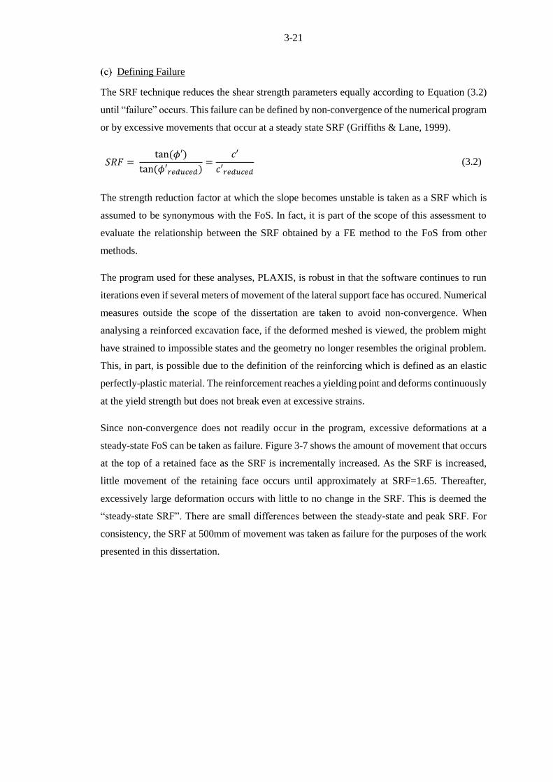
3-21
Defining Failure
The SRF technique reduces the shear strength parameters equally according to Equation (3.2)
until “failure” occurs. This failure can be defined by non-convergence of the numerical program
or by excessive movements that occur at a steady state SRF (Griffiths & Lane, 1999).
𝑆𝑅𝐹 = tan (𝜙′)
tan (𝜙′𝑟𝑒𝑑𝑢𝑐𝑒𝑑)=
𝑐′
𝑐′𝑟𝑒𝑑𝑢𝑐𝑒𝑑 (3.2)
The strength reduction factor at which the slope becomes unstable is taken as a SRF which is
assumed to be synonymous with the FoS. In fact, it is part of the scope of this assessment to
evaluate the relationship between the SRF obtained by a FE method to the FoS from other
methods.
The program used for these analyses, PLAXIS, is robust in that the software continues to run
iterations even if several meters of movement of the lateral support face has occured. Numerical
measures outside the scope of the dissertation are taken to avoid non-convergence. When
analysing a reinforced excavation face, if the deformed meshed is viewed, the problem might
have strained to impossible states and the geometry no longer resembles the original problem.
This, in part, is possible due to the definition of the reinforcing which is defined as an elastic
perfectly-plastic material. The reinforcement reaches a yielding point and deforms continuously
at the yield strength but does not break even at excessive strains.
Since non-convergence does not readily occur in the program, excessive deformations at a
steady-state FoS can be taken as failure. Figure 3-7 shows the amount of movement that occurs
at the top of a retained face as the SRF is incrementally increased. As the SRF is increased,
little movement of the retaining face occurs until approximately at SRF=1.65. Thereafter,
excessively large deformation occurs with little to no change in the SRF. This is deemed the
“steady-state SRF”. There are small differences between the steady-state and peak SRF. For
consistency, the SRF at 500mm of movement was taken as failure for the purposes of the work
presented in this dissertation.

3-22
Figure 3-7: Strength Reduction Factor against horizontal movement of the top anchor
head
0
500
1000
1500
2000
2500
3000
3500
0.9 1.0 1.1 1.2 1.3 1.4 1.5 1.6 1.7
Hori
zonta
l m
ovem
ent
of
top a
nch
or
(mm
)
SRF
1.649
1.651
1.641
Peak SRF
500mm SRF
Steady-state SRF


CHAPTER 4 ANALYSIS RESULTS AND DISCUSSION
Four different methods of analysis are applied to three different cases / geometries. In this
chapter, the results of the analyses performed are presented. The first case analysed is the
stability analysis of a simple unreinforced slope to investigate the impact of the method of
analysis on a stability problem without involving any complexities associated with
reinforcement. The stability of two vertical excavations, reinforced using soil-nails and anchors
respectively, is then presented. At the end of the chapter, a discussion on the major differences
between various methods of analysis is presented.
4.1 UNIFORM SLOPE
Some analysis techniques for laterally supported excavations originate from slope stability
applications. It was, therefore, decided to first investigate a basic slope stability problem and
consider the differences between the methods without the complexities involved with the
inclusion of soil-nails and anchors. A simple, 15m high, 1:2 (26.6°) gradient, uniform slope
was analysed using the several methods of analysis. Consider a 1:2 slope as illustrated in Figure
4-1. The four different methods of analysis and the software packages used to calculate the
Factor of Safety (FoS) against slope failure are summarised in Table 4-1.
Table 4-1: Different methods of analysis
Method of Analysis Software / Program Abbreviation
1. Limit Equilibrium – Single Trial
Wedge Failure Microsoft Excel Wedge
2. Limit Equilibrium – Method of
Slices SLOPE/W MoS
3. Enhanced Limit Equilibrium
SIGMA/W &
SLOPE/W ELE
4. Finite Element – Strength
Reduction Factor PLAXIS 2D FE (SRF)
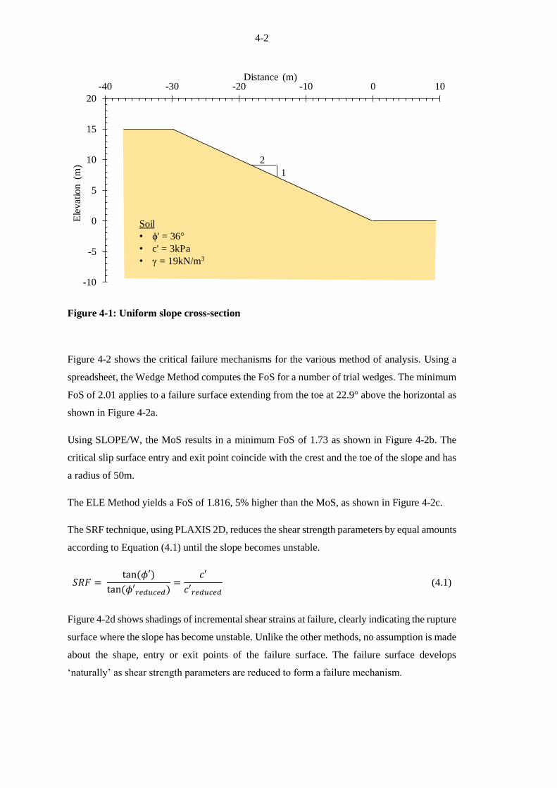
4-2
Figure 4-1: Uniform slope cross-section
Figure 4-2 shows the critical failure mechanisms for the various method of analysis. Using a
spreadsheet, the Wedge Method computes the FoS for a number of trial wedges. The minimum
FoS of 2.01 applies to a failure surface extending from the toe at 22.9° above the horizontal as
shown in Figure 4-2a.
Using SLOPE/W, the MoS results in a minimum FoS of 1.73 as shown in Figure 4-2b. The
critical slip surface entry and exit point coincide with the crest and the toe of the slope and has
a radius of 50m.
The ELE Method yields a FoS of 1.816, 5% higher than the MoS, as shown in Figure 4-2c.
The SRF technique, using PLAXIS 2D, reduces the shear strength parameters by equal amounts
according to Equation (4.1) until the slope becomes unstable.
𝑆𝑅𝐹 = tan (𝜙′)
tan (𝜙′𝑟𝑒𝑑𝑢𝑐𝑒𝑑)=
𝑐′
𝑐′𝑟𝑒𝑑𝑢𝑐𝑒𝑑 (4.1)
Figure 4-2d shows shadings of incremental shear strains at failure, clearly indicating the rupture
surface where the slope has become unstable. Unlike the other methods, no assumption is made
about the shape, entry or exit points of the failure surface. The failure surface develops
‘naturally’ as shear strength parameters are reduced to form a failure mechanism.
-10
-5
0
5
10
15
20
-40 -30 -20 -10 0 10E
lev
atio
n (
m)
Distance (m)
2
1
Soil
• ϕ' = 36°
• c' = 3kPa
• γ = 19kN/m3

4-3
Both the MoS and ELE Method use the normal stress on a failure surface to calculate the FoS.
To obtain the normal force, the MoS uses the weight of a vertical slice together with some
assumption made regarding the inter-slice forces. The ELE Method uses a finite element model
to calculate these stresses. The distribution of normal stress on the slip surface is shown in
Figure 4-3 for the MoS and the ELE Method. The ELE Method obtains a slightly different
distribution of normal stress, especially at the ends of the slip surface domain, resulting in a
higher FoS.
a. Wedge Method (FoS = 2.01) b. Method of Slices (FoS = 1.73)
c. Enhanced Limit Equilibrium (FoS = 1.82) d. Finite Element (SRF) (FoS = 1.72)
Figure 4-2:Uniform slope critical failure mechanisms and associated factors of safety
Figure 4-3: Normal stress distribution along slip surface
-10
-5
0
5
10
15
20
-55 -50 -45 -40 -35 -30 -25 -20 -15 -10 -5 0 5 10 15
Ele
vat
ion
(m
)
Distance (m)
Critical Failure Surface, 22.9°
Slope, 26.6°
FoS = 2.01
26.6°
-10
-5
0
5
10
15
20
-55 -50 -45 -40 -35 -30 -25 -20 -15 -10 -5 0 5 10 15
Ele
vat
ion (
m)
Distance (m)
FoS = 1.73
-10
-5
0
5
10
15
20
-55 -50 -45 -40 -35 -30 -25 -20 -15 -10 -5 0 5 10 15
Ele
vat
ion
(m
)
Distance (m)
FoS = 1.82
-10
-5
0
5
10
15
20
-55 -50 -45 -40 -35 -30 -25 -20 -15 -10 -5 0 5 10 15
Ele
vat
ion
(m
)
Distance (m)
FoS = 1.72
0
10
20
30
40
50
60
0 5 10 15 20 25 30
Bas
e N
orm
al S
tres
s (k
Pa)
Distance (m)
ELE
MoS
MoS: FoS = 1.73
ELE: FoS = 1.82

4-4
The various FoS obtained from the different methods are summarised in Figure 4-4. The Wedge
Method yields a FoS of 2.01, higher than the other methods. The MoS results in a FoS = 1.73.
The ELE Method, which aims to calculate a more accurate distribution of stress at the slip
surface, yields a FoS 5% higher than the conventional MoS. A maximum SRF of 1.75 was
obtained using a FE (SRF) Method, close to the FoS determined from the MoS. The failure
mechanism of the FE (SRF) Method agrees well with the MoS and ELE Method. The planar
trial Wedge Method failure mechanism does not suit gently inclined slope problems, yielding
on a FoS 10 – 15% higher than the other methods. The presence of cohesion in soil also favours
curved failure mechanisms which is not captured by the Wedge Method.
Figure 4-4: Minimum FoS obtained from various methods for uniform slope
2.01
1.73
1.81
1.72
1.4
1.5
1.6
1.7
1.8
1.9
2
2.1
2.2
LE (Wedge) LE (MoS) ELE FE (SRF)
Fac
tor
of
Saf
ety
Method Used

4-5
4.2 SOIL-NAILED EXCAVATION
As part of the study, two different lateral support designs for vertical excavations were
evaluated in terms of limit equilibrium and finite element methods. These designs encompass
soil-nails and anchors respectively. The first design is of an 8.5m deep retained face using soil-
nails and is reported in this section. In the next section, a 17m vertical face supported using
anchors is discussed. In analysing these two unique, yet typical scenarios, an attempt is made
to get a better understanding of the sensitivity of the FoS to various model, material and design
variables.
4.2.1 Introduction
The geometry of the soil-nailed excavation consists of an 8.5m high vertical cut. A photograph
site during constriction is shown in Figure 4-5. Cross-section A-A is superimposed on the right-
hand side of the figure with the engineering detail shown in Figure 4-6.
Figure 4-5: Soil-nailed excavation during construction with cross-section A-A

4-6
Figure 4-6: Cross-section A-A showing soil-nailed details
After the geotechnical investigation, parameters were determined for the design of the lateral
support system. A discussion of the material parameters used is given in Section 3.2.1 with a
summary of the values used repeated below in Table 4-2. A discussion of the design parameters
is presented in Section 3.2.3. An initial design was carried out based on a trial wedge limit
equilibrium analysis with a target FoS of 1.5, a value recommended for permanent lateral
support (SAICE, 1989). Based on this initial target, 5 rows of 6m-length, 20mm-diameter soil-
nails were selected, spaced horizontally at 1.5m.
-2
0
2
4
6
8
10
-4 -2 0 2 4 6 8 10 12
Ele
vat
ion (
m)
Distance (m)
100mm shotcrete
10°
8.5m
7.0m
5.5m
4.0m
2.5m
1.0m
0m
Soil-nail bars:
• 6m length
• 20mm diameter
• Sv = Sh = 1.5m
Soil
• ϕ' = 36°
• c' = 3kPa
• γ = 19kN/m3

4-7
Table 4-2: Material parameters used for modelling of soil-nailed excavation
Parameter Units Value
Friction Angle, ϕ' ° 36
Cohesion, c' kPa 3
Unit weight, γ kN/m3 19
Poisson’s ratio, v' 0.3
Stiffness, E’ MPa 90
Angle of dilation, ψ' ° 18
Soil model
Elastic-Plastic (Mohr-
Coulomb yield
criterion)
4.2.2 Factor of safety from different methods of analysis
The FoS for the different methods of analysis are plotted in Figure 4-7 against the slope angle
of the failure mechanism (assuming a straight line between entry and exit points where curved
failure surfaces are predicted). The minimum FoS obtained for each of the various methods are
shown in Figure 4-8. The failure mechanisms yielding the critical FoS is shown in Figure 4-9.
The Wedge Method results in a minimum FoS of 1.58 which is close to that of 1.63 obtained
using the MoS. The ELE Method computes in a FoS of 1.43, lower than the methods above.
The failure surface of the ELE Method is shallower than the other three methods. The FE (SRF)
Method results in a FoS of 1.42, comparable to the ELE Method, but the slope of the failure
mechanism is similar to the limit equilibrium methods. The reason and explanations for the
differences in FoS and failure mechanisms are discussed in subsequent sections.
Figure 4-7: Factor of safety for various slip angles
LE (Wedge), 1.58
LE (MoS), 1.63
ELE, 1.43FE (SRF), 1.42
0
0.5
1
1.5
2
2.5
3
30 35 40 45 50 55 60 65 70
Fac
tor
of
Saf
ety
Slip angle above horizontal, β (deg)
LE (Wedge)
LE (MoS)
ELE
FE (SRF)

4-8
Figure 4-8: Minimum FoS obtained from various method for soil-nailed excavation
a. Wedge Method (FoS = 1.58) b. Method of Slices (FoS = 1.63)
c. Enhanced Limit Equilibrium (FoS = 1.43) d. Finite Element (SRF) (FoS = 1.42)
Figure 4-9: Soil-nailed excavation critical failure mechanisms and associated factors of
safety
1.58
1.63
1.43 1.42
1.2
1.3
1.4
1.5
1.6
1.7
1.8
LE (Wedge) LE (MoS) ELE FE (SRF)
Fac
tor
of
Saf
ety
Method Used
-3
-2
-1
0
1
2
3
4
5
6
7
8
9
10
-6 -4 -2 0 2 4 6 8 10 12 14
Ele
vat
ion (
m)
Distance (m)
FoS = 1.58
-3
-2
-1
0
1
2
3
4
5
6
7
8
9
10
-6 -4 -2 0 2 4 6 8 10 12 14
Ele
vat
ion (
m)
Distance (m)
FoS = 1.63
-3
-2
-1
0
1
2
3
4
5
6
7
8
9
10
-6 -4 -2 0 2 4 6 8 10 12 14
Ele
vat
ion (
m)
Distance (m)
FoS = 1.43
-3
-2
-1
0
1
2
3
4
5
6
7
8
9
10
-6 -4 -2 0 2 4 6 8 10 12 14
Ele
vat
ion (
m)
Distance (m)
FoS = 1.42

4-9
4.2.3 Effects of model geometry and mesh on FoS - ELE Method
When setting up a finite element model, the boundary distances and meshing are two important
factors that could influence the accuracy of the computed FoS. This is applicable to both the
ELE and FE (SRF) Methods since both make use of discretised meshes.
Meshing
A trade-off between calculation time and accuracy has to be made in setting up the correct
mesh. In general, the finer the mesh, the better the numerical accuracy of the results, but this
comes at the expense of calculation time.
The number of elements within a standard model size is used here as an indicator of the mesh
resolution. Figure 4-10 shows the FoS obtained by increasing the number of mesh elements
i.e. decreasing the mesh size. The FoS approaches a steady-state value as the mesh is refined.
In this case, a uniform element size meshing strategy was chosen i.e. all the elements are
approximately the same size throughout the model.
Figure 4-10: FoS against number of elements for a global mesh size
Generally, it is computationally inefficient to select a globally uniform mesh size. It would be
prudent to use a finer mesh near the soil-nails and shotcrete wall where the majority of the
deformation will occur and a coarser mesh towards the boundaries. Figure 4-11 shows the mesh
in the FE model for such a ‘graded meshing strategy’. Figure 4-12 shows a comparison between
selecting a uniform mesh size versus finer mesh near critical elements. It can be seen that the
steady-state FoS of 1.42 is reached at only 6 000 elements, whereas a uniform mesh size would
1.4201.423
1.4371.440
1.459
1.490
1.35
1.4
1.45
1.5
1.55
0 20000 40000 60000 80000 100000 120000
Fac
tor
of
Saf
ety
Number of Elements
ELE

4-10
require over 30 000 elements to provide a similar answer. The number of elements is
proportional to the calculation time and thus a graded mesh should be chosen.
Figure 4-11: Graded meshing model for ELE Method
Figure 4-12: FoS against number of elements for a global mesh size versus graded
meshing
-25
-20
-15
-10
-5
0
5
10
-30 -20 -10 0 10 20 30 40
Ele
vat
ion (
m)
Distance (m)
1.423
1.4371.440
1.459
1.490
1.440
1.425 1.424
1.35
1.4
1.45
1.5
1.55
0 10000 20000 30000 40000 50000 60000 70000 80000
Fac
tor
of
Saf
ety
Number of Elements
ELE - Global Meshing
ELE - Graded Meshing

4-11
Boundary distance
Another important consideration is the distances of the boundaries from the excavation face in
the finite element model. Boundary conditions that are too close will impose some constraints
affecting the deformation of the soil. The model cross-sectional area is used as an indicator of
the boundary distances. In Figure 4-13, a model is shown having a cross-sectional area of
2 010m2. Although a modeller might intuitively feel that the boundary conditions are
sufficiently far away, Figure 4-14 shows a significant increase in the FoS as the model cross-
sectional area is increased, i.e. the left, right and bottom boundaries are moved further away
from the excavation face. Boundary distances were increased at the same increments and the
FoS observed.
As the boundary distances are increased, resulting in an increased model cross-sectional area,
the rate of change in FoS decreases. However, even at a model cross-sectional area of 9 000m2
(i.e. left and bottom boundaries - 60m from the toe & right boundary - 70m from the toe) the
FoS still seems to increase. For the purposes of the analysis described hence forth a model with
a cross-sectional area of approximately 4 400m2 was chosen, yielding a FoS of 1.43. Boundaries
encroaching on the excavation face results in confinement which generally increases the stress
within the soil mass. Since, the FoS formulation of the ELE Method compares the ratio of
computed to the available stress, confinement results in a decrease in FoS.
Figure 4-13: Model of cross-sectional area of 2 010m2
-25
-20
-15
-10
-5
0
5
10
-30 -20 -10 0 10 20 30 40
Ele
vat
ion (
m)
Distance (m)

4-12
Figure 4-14: FoS as function of the model cross-sectional area
4.2.4 Effects of model geometry and mesh on FoS - FE (SRF) Method
Meshing
Previously, for the ELE model, a global mesh size was compared to a graded meshing strategy
which was shown to be more efficient, considering the complex deformations in the vicinity of
the soil-nails. In the case of the FE model for SRF analysis, the influence of a meshing strategy
(global or graded) or resolution (course or fine) does not seem as apparent. Figure 4-15 shows
the influence of the mesh resolution on the FoS. Neither the number of elements nor the
meshing strategy has a significant impact on the FoS outcome.
The FE (SRF), using PLAXIS software, uses 15-noded, higher order, triangular elements
instead of the 4-noded quadrilateral elements used by SIGMA/W for the ELE Method. PLAXIS
(2016) emphasises the benefit of using 15-noded element with the only drawback being
calculation time. It is well known that the element type influences the FoS (Tschuchnigg et al.
2015; Sloan & Randolph, 1982) and in this case the use of higher order elements, cause rapid
convergence to a steady state FoS.
1.297
1.378
1.4121.425
1.4441.457
1.2
1.25
1.3
1.35
1.4
1.45
1.5
1.55
0 1000 2000 3000 4000 5000 6000 7000 8000 9000 10000
Facto
r of
Safe
ty
Model Area (m2)
ELE

4-13
Figure 4-15: FoS against number of elements for a global mesh size versus graded
meshing for FE (SRF) model
Boundary distances
Distances to the model boundaries were again varied to analyse the influence on the FoS. Figure
4-16 shows the influence of boundary distances on the FoS. In the case of the FE (SRF) model,
the boundary distances were found not to have an influence on the FoS.
Boundaries were chosen for a model resulting in a cross-sectional area of 2 010m2. Left and
bottom boundaries were spaced equidistant from the toe of the wall at a distance of 25m. An
additional 10m was allowed for the right-hand side boundary for the influence of the nails. A
measure of the model proportion is the boundary distance ÷ wall height (25 / 8.5) = 2.9.
A model comprising 5198 elements (42 647 stress points) and a cross-sectional area of 2 010m2
selected for the analyses that follow, although a coarser model could well have been selected.
The model cross-section used for further analyses is shown in Figure 4-17.
1.45 1.451.43 1.44
1.451.44
1.43
1.35
1.4
1.45
1.5
1.55
0 2000 4000 6000 8000 10000 12000 14000 16000
Fac
tor
of
Saf
ety
Number of Elements
FE (SRF) - Global Meshing
FE (SRF) - Graded Meshing

4-14
Figure 4-16: FoS against number of elements for a global mesh size
Figure 4-17: FE (SRF) graded mesh model with 2 010m2 cross-sectional area and 5 198
elements
1.441.45 1.45
1.35
1.4
1.45
1.5
1.55
0 500 1000 1500 2000 2500 3000
Fac
tor
of
Saf
ety
Model Area (m²)
-25
-20
-15
-10
-5
0
5
10
-30 -20 -10 0 10 20 30 40
Ele
vat
ion (
m)
Distance (m)

4-15
4.2.5 Effect of material properties on FoS
Selection of the correct material properties is essential for the accuracy of the stability
calculation irrespective of the method used. This section reports the impact of material
parameter choice on the computed FoS using four methods of analysis.
For each of the material properties investigated, four plots are shown based on the various
methods of analysis used:
Wedge: limit equilibrium trial Wedge Method
MoS: limit Equilibrium Method of Slices
ELE: Enhanced Limit Equilibrium Method
FE (SRF): Finite Element method using the Strength Reduction Factor technique.
In Section 4.2.2, the minimum FoS for each of the four methods was pointed out. This FoS is
obtained using the baseline soil parameters as defined Section 4.2.1. In the subsections that
follow, parameters applicable to the Mohr-Coulomb soil model is varied (reduced and
increased) to analyse the influence of soil parameters on FoS. All four methods use a Mohr-
Coulomb failure criterion defined by the soil friction angle (ϕ'), cohesion (c') and unit weight
(γ). For the ELE and FE (SRF) Methods, the pre-failure deformation characteristics, Young’s
modulus (E') and Poisson’s ratio (v'), were also investigated.
Friction angle
The influence of soil’s internal angle of friction, ϕ', on the FoS is shown Figure 4-18. Unlike
the pre-failure deformation characteristics, E' and v', the friction angle has a controlling
influence on limit equilibrium, ELE and FE (SRF) Methods.
For the limit equilibrium methods (Wedge and MoS), the resistance against slip is calculated
as normal force at the base of the slip multiplied by tanϕ' and, as expected, the limit equilibrium
FoS increases with an increase in friction angle. The Wedge and MoS compute similar FoS,
with the Wedge Method being slightly higher.
For the ELE Method, the above also applies in part, since ultimately, a limit equilibrium
analysis is also carried out. The primary difference is that for a limit equilibrium analysis, the
stresses at the slip surface are simply determined from the weight of soil above the slice/wedge
and for the ELE Method these stresses are calculated from an elastic-plastic finite element
analysis using a Mohr-Coulomb soil model. The initial stresses were obtained using a single
stage ‘gravity turn-on’ procedure. The influence of modelling construction sequences is later
discussed.

4-16
For the ELE Method, a change in friction angle appears somewhat less significant than for the
other methods. The FoS ranges from 1.15 – 1.52 for friction angles of 25° - 40°. The in-situ
stress state defined by a Poisson’s ratio of v' = 0.3 was kept constant. This resulted in the in-
situ stress state exceeding the yield criterion at ϕ' = 20°. At high friction angles, the ELE
Method seems to predict lower FoS than the other methods and is therefore conservative. At
low friction angles the opposite is observed.
The FoS calculated using the FE (SRF) Method follows the same trend as the limit equilibrium
methods. However, at friction angles, ϕ' = 20° and ϕ' = 25°, the FoS is below unity, indicating
a failure state. Before the strength reduction technique is applied, PLAXIS uses a procedure
incrementally increasing gravity from weightless to 100% to ensure stability is indeed achieved
– that is, a FoS of 1.0 is reached. For a FoS less than unity the strength reduction procedure is
not applied and a FoS is not computed. At a friction angle ϕ' = 25°, loading occurs to 97% of
soil unit weight before failure occurs and is included in the figure as a FoS = 0.97 only for
comparison. The FoS for the FE (SRF) Method is between 0.12 and 0.21 less than the limit
equilibrium methods.
Figure 4-18: FoS for a change in soil friction angle, ϕ'
0.84
1.81
0.87
1.87
1.15
1.52
0.97
1.16
1.66
0.8
1
1.2
1.4
1.6
1.8
2
15 20 25 30 35 40 45
Fac
tor
of
Saf
ety
Friction Angle, ϕ' (deg)
LE (Wedge)
LE (MoS)
ELE
FE (SRF)
In-situ Stress
Violation
No SRF
Applied

4-17
Cohesion
The ‘cohesion’ refers to the intercept of the Mohr-Coulomb failure envelope on the shear
strength axis. At a given normal stress, a soil element has an increased shear strength owing to
cohesion. The cohesion (actual or apparent) can be as a result of a host of factors including
suction, cementation and particle interlock.
Figure 4-19 shows the FoS against a change on soil cohesion. An increase in the cohesive
strength of a material results in an increase in the FoS, irrespective of the method used. The
difference in FoS between the Wedge, MoS and FE (SRF) Methods remains constant with
increasing cohesion. The FoS increases by approximately 0.1 for every 3kPa of cohesive
strength for the geometry analysed. The ELE Method predicts the lowest FoS at high cohesion
values. The results illustrate the large effect that cohesion has on the calculated FoS which
emphasises the importance of choosing this parameter carefully.
Figure 4-19: FoS for a change in cohesion, c'
1.82
1.53
1.63
1.70
1.86
1.57
1.30
1.70
1.2
1.3
1.4
1.5
1.6
1.7
1.8
1.9
0 2 4 6 8 10 12
Fac
tor
of
Saf
ety
Cohesion, c' (kPa)
LE (Wedge)
LE (MoS)
ELE
FE (SRF)

4-18
Unit weight
The unit weight has a dual effect on the FoS by increasing both the normal force on the slip
surface providing stability and the driving force along the slip surface causing failure. However,
since the system, without the addition of reinforcing, is not in static equilibrium – that is, there
is a deficit in force/moment resistance – the unit weight further increases this deficit which
reduces the FoS.
A decrease in FoS is seen for limit equilibrium and FE (SRF) Methods. The Wedge and MoS
differ slightly, with the Wedge Method computing a higher FoS. Both limit equilibrium
methods compute FoS higher than the ELE and FE (SRF) Methods, however, the difference
decreases with an increase in unit weight.
No change is seen in the ELE Method for a change in material unit weight. The reason for this
can be explained with the failure mechanism which is discussed later in Section 4.3.5.
Figure 4-20: FoS for a change in soil unit weight, γ
1.76
1.48
1.83
1.63
1.52
1.441.43
1.53
1.441.38
1.2
1.3
1.4
1.5
1.6
1.7
1.8
1.9
15 16 17 18 19 20 21 22
Fac
tor
of
Saf
ety
Unit Weight, γ (kN/m³)
LE (Wedge)
LE (MoS)
ELE
FE (SRF)

4-19
Young’s modulus
The Young’s modulus, E', is a major contributor to the stiffness of the system being analysed.
A high Young’s modulus value translates directly to small amount of movements causing a
large change in stress.
Figure 4-21 shows the FoS computed for a range of Young’s moduli. The limit equilibrium
methods are independent of Young’s modulus because no stress-strain relationship is required.
Their FoS is shown for comparison.
The ELE Method shows a decrease in FoS as the Young’s modulus increases. Note that
Young’s modulus is independent of the material strength.
Young’s modulus does not seem to have an influence on the FoS of the FE (SRF) Method. A
possible reason for this is that the strength reduction factor is only concerned with failure, where
Young’s modulus only applies to pre-failure stresses.
Figure 4-21: FoS for a change in Young’s Modulus, E'
1.58
1.63
1.48
1.31
1.43 1.43
1.2
1.25
1.3
1.35
1.4
1.45
1.5
1.55
1.6
1.65
1.7
10 100 1000
Fac
tor
of
Saf
ety
Young's Modulus, E' (MPa)
LE (Wedge)
LE (MoS)
ELE
FE (SRF)

4-20
Poisson’s ratio
As with the Young’s modulus, the limit equilibrium methods are independent of the Poisson’s
ratio as these methods do not consider stiffness parameters. Figure 4-22 shows the change in
FoS for a range of Poisson’s ratio values. The ELE Method FoS fluctuates with a variation in
Poisson’s ratio. The FE (SRF) Method shows no significant change in FoS for a change in the
Poisson’s ratio.
The ELE Method, analysed using SIGMA/W, uses the 1-Dimensional elastic compression
equation (K0 = v' / 1-v') to calculate the in-situ coefficient of lateral earth pressure as a function
of the Poisson ratio. The relationship between Poisson’s ratio and the in-situ coefficient of
lateral earth pressure at-rest, K0, is graphically shown in Figure 4-23. The FE (SRF) Method,
analysed using PLAXIS, uses Jaky’s equation (K0 = 1 – sinϕ') (Jaky, 1944) to calculate the in-
situ horizontal stresses. Regardless of the method used, an in-situ stress ratio should be specified
in such a way so that the stress state does not violate the Mohr-Coulomb yield criterion. This
will cause the entire soil mass to be in a state of yielding, i.e. plastic deformation already in the
in-situ state. In the case of an elastic-plastic soil model this will result in material behaviour
being modelled using equations of plasticity instead of elasticity.
In Figure 4-22, for the ELE Method, two points at v = 0.15 and v = 0.2 are highlighted, which
violate the yield criterion. This is the reason causing the relationship between the FoS and the
Poisson ratio to deviate from the general trend of the curve in the figure. The situation of in-
situ stresses violating the yield criterion is further discussed in Section 4.4.1.
Figure 4-22: FoS for a change in the Poisson’s ratio, v'
1.58
1.63
1.39
1.43
1.43
1.2
1.25
1.3
1.35
1.4
1.45
1.5
1.55
1.6
1.65
1.7
0 0.05 0.1 0.15 0.2 0.25 0.3 0.35 0.4 0.45 0.5
Fac
tor
of
Saf
ety
Poisson's Ratio, v
LE (Wedge)
LE (MoS)
ELE
FE (SRF)
In-situ Stress
Violation

4-21
Figure 4-23: In-situ stress ratio, K0, values for specified Poisson, v', using 1-Dimensional
compression
4.2.6 Effect of reinforcement length and bar diameter on FoS
When considering the internal stability of an excavation, yielding and pull-out of soil-nails are
the primary failure mechanisms. Other modes of failure do exist, such as the nail punching
through the shotcrete face but this is beyond the scope of this research and was not considered.
The yield capacity of the bar is dependent on its yield stress and the diameter of the selected
steel bar. The pull-out resistance is dependent on the hole diameter and the length of bar behind
the failure surface and is independent of the bar diameter. The yield stress of the reinforcing
bar and hole drilling diameter considered are 500MPa and 102mm (4'') respectively (Section
3.2.3).
The designer must select the bar diameter and length in order to provide an adequate FoS for
the excavation under consideration. In this section, the influence of the bar length and diameter
are discussed.
Soil-nail bar diameter
Increasing the soil-nail bar diameter increases the FoS as seen in Figure 4-24 for the limit
equilibrium, ELE and FE (SRF) Methods. For the limit equilibrium and FE (SRF) Methods,
there is a distinct slope change in the curves which represent the point where all nails are now
subject to a pull-out failure mechanism. Increasing the bar diameter beyond this point has no
0
0.2
0.4
0.6
0.8
1
1.2
0 0.05 0.1 0.15 0.2 0.25 0.3 0.35 0.4 0.45 0.5
In-s
itu S
tres
s R
atio
, K
0(v
/ 1
-v)
Poisson's Ratio, v

4-22
benefit from a stability point of view since the pull-out resistance is a function of the drilling
diameter which stays constant. Using the limit equilibrium trial Wedge Method, this point
occurs at a bar diameter of 21mm for the geometry analysed. An increase in diameter from
16mm to 20mm results in an increase in the FoS of 0.22 and 0.25 for the Wedge Method and
the MoS respectively.
Figure 4-24: FoS for a change in nail diameter.
Soil-nail reinforcement length
Increasing the reinforcement length results in a longer length of reinforcing behind the failure
surface which increases the total pull-out force. Figure 4-25 shows the change in FoS for change
in soil-nail length. The FoS increases for an increase in nail length for all methods except the
ELE Method which remains constant at a FoS of 1.43. The Wedge Method and MoS closely
follow each other as seen with many of the other investigations. A divergence is seen between
the limit equilibrium methods and the FE (SRF) curves and a difference in FoS of up to 0.5 is
observed at a reinforcing length of 8m.
In a similar fashion to the bar diameter, an increase in nail length will only be effective to the
point where all nails fail in tension by yielding. Using the Wedge Method and the assumed
bond strength (110kPa or 35kN/m), this point occurs at a nail length of between 9 and 10m
(FoS = 2.58). The same is observed for the FE (SRF) Method, where little benefit in FoS is
seen beyond a soil-nail length of 9m (FoS = 1.80).
1.36
1.65
1.38
1.63
1.73
1.73
1.41
1.50
1.29
1.421.42
1.2
1.3
1.4
1.5
1.6
1.7
1.8
10 15 20 25 30 35 40
Fac
tor
of
Saf
ety
Soil-Nail Bar Diameter (mm)
LE (Wedge)
LE (MoS)
ELE
FE (SRF)

4-23
Figure 4-25: FoS for a change nail design length
Increasing nail diameter versus increasing nail length
The cost of reinforcement is a function of the mass of steel, which is directly proportional to
the bar cross-sectional area, not the bar diameter. An increase in FoS of 0.22 and 0.25, for the
Wedge Method and MoS respectively, is observed by increasing the bar cross-sectional area
from 201mm2 to 314mm2 (16mm to 20mm diameter). This equates to an increase in the FoS of
approximately 0.04 for every 10% of additional reinforcement cross-sectional area (or mass).
The mass of steel is directly proportional to the soil-nail bar length. By increasing the
reinforcement length, for the Wedge Method and MoS, the FoS increases linearly at a rate of
0.14 for every 10% increase in length (or mass).
A greater positive impact is seen on the FoS by increasing the nail length in comparison to
increasing the nail cross-sectional area (i.e. the nail diameter). Therefore, an increase in length
of reinforcement is more beneficial than increasing the nail diameter in terms of cost of
reinforcement.
The reason for the advantage is that at failure of 6m-long, 20mm-diameter soil-nails (baseline
parameters), the top 4 soil-nails fail by pulling-out and the bottom nail fails due to yielding.
Therefore, increasing the bar diameter is only benefitting the bottom nail until a point where it
also fails due to pull-out. Increasing the nail length benefits the top 4 soil-nails until they all
fail due to yielding.
1.30
2.15
2.58
1.36
2.21
1.42 1.43
1.25
1.42
1.71
1.82
1.2
1.4
1.6
1.8
2
2.2
2.4
2.6
2.8
4 5 6 7 8 9 10 11
Fac
tor
of
Saf
ety
Soil-Nail Length (m)
LE (Wedge)
LE (MoS)
ELE
FE (SRF)
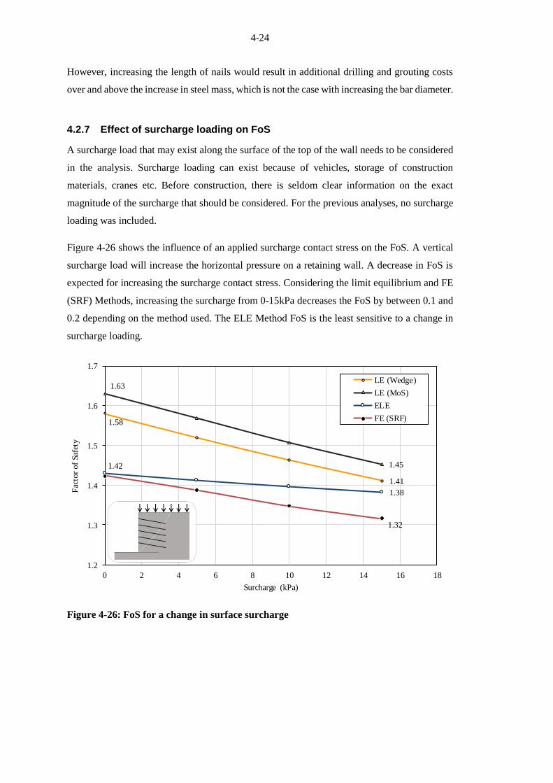
4-24
However, increasing the length of nails would result in additional drilling and grouting costs
over and above the increase in steel mass, which is not the case with increasing the bar diameter.
4.2.7 Effect of surcharge loading on FoS
A surcharge load that may exist along the surface of the top of the wall needs to be considered
in the analysis. Surcharge loading can exist because of vehicles, storage of construction
materials, cranes etc. Before construction, there is seldom clear information on the exact
magnitude of the surcharge that should be considered. For the previous analyses, no surcharge
loading was included.
Figure 4-26 shows the influence of an applied surcharge contact stress on the FoS. A vertical
surcharge load will increase the horizontal pressure on a retaining wall. A decrease in FoS is
expected for increasing the surcharge contact stress. Considering the limit equilibrium and FE
(SRF) Methods, increasing the surcharge from 0-15kPa decreases the FoS by between 0.1 and
0.2 depending on the method used. The ELE Method FoS is the least sensitive to a change in
surcharge loading.
Figure 4-26: FoS for a change in surface surcharge
1.58
1.41
1.63
1.45
1.38
1.42
1.32
1.2
1.3
1.4
1.5
1.6
1.7
0 2 4 6 8 10 12 14 16 18
Fac
tor
of
Saf
ety
Surcharge (kPa)
LE (Wedge)
LE (MoS)
ELE
FE (SRF)

4-25
4.2.8 Modelling of construction sequence
For all of the previous analyses, a single excavation stage was assumed and the FoS was
computed at the final excavation level. In reality, this is not the case. Excavation occurs
progressively in stages and not instantaneously. Two aspects are important when considering
modelling of construction sequencing:
a) FoS throughout construction process. The FoS needs to be sufficient throughout the
entire construction process and not just at the final excavation level.
b) Influence of construction sequence modelling on final FoS. A check needs to be carried
out to see if there is a difference in FoS obtained at final excavation level when
modelling a single excavation or a construction sequence.
FoS throughout construction process
Figure 4-27 is a process diagram of the construction sequence modelling. In the first phase
(Phase 0) the in-situ stresses are calculated dependent on the governing K0 function. Once
excavation has taken place at any level, the face is temporarily exposed until a soil-nail for that
excavation lift is installed. The FoS can be calculated at the end of the excavation phase where
the face is temporarily exposed (this is indicated as Phase 1A, 2A etc.). The FoS can again be
evaluated once the soil-nail at this elevation has been installed, which will of course be higher,
given the same retained height which now includes an additional soil-nail (Phase 1B, 2B etc.).
Theoretically, with too low cohesion values, it is impossible for a vertically exposed face of a
few meters high to be stable. Temporary stability could be provided by matric suctions (beyond
the scope of this dissertation). For the purposes in this dissertation, the local stability of the
temporary exposed portion before installation of the soil-nail was not assessed, however, the
global stability was calculated. Also, the FoS of the first excavation without the presence of
any soil-nails (Phase 1A) was omitted. It is up the designer to judge if these temporary scenarios
are critical.
Figure 4-28 shows the FoS as a function of excavation depth for the Wedge Method and MoS.
As previously explained, the FoS for the ‘excavation phase’ and ‘nail installed’ phase are noted
separately for each excavation lift.
A decrease in the FoS is observed as the depth of the excavation increases. At shallow
excavation depths, the FoS calculated from the Wedge Method deviates from the MoS, which
calculates a lower FoS. For all construction phases, the minimum FoS = 1.46 occurs at an
excavation depth of 8m before the final soil-nail is installed. Excluding this temporary case, the
minimum FoS occurs at final depth.

4-26
Figure 4-27: Construction sequence of soil-nailed excavation
Figure 4-28: FoS against excavation depth for Wedge Method and MoS
“Final” FoS
Phase 0: In-situ Stresses
Phase 1A: Excavate to 2.0m
Phase 1B: Install Nail at 1.5m
Phase 2A: Excavate to 3.5m
Phase 2B: Install Nail at 3.0m
“Excavation Phase” FoS
“Nail Installed” FoS
“Nail Installed” FoS
Phase 5A: Excavate to 8.0m
Phase 5B: Install Nail at 7.5m “Nail Installed” FoS
Phase 6A: Excavate to 8.5m
. . .
“Excavation Phase” FoS
“Excavation Phase” FoS
4.49
1.58
5.39
1.63
3.60
2.84
1.46
1
1.5
2
2.5
3
3.5
4
4.5
5
5.5
6
0 0.5 1 1.5 2 2.5 3 3.5 4 4.5 5 5.5 6 6.5 7 7.5 8 8.5 9
Facto
r of
Safe
ty
Excavation Depth (m)
LE (Wedge) - Nail Installed LE (MoS) - Nail Installed
LE (Wedge) - Excavation Phase LE (MoS) - Excavation Phase
Nail InstalledExcavation Phase

4-27
Figure 4-29 shows the FoS as a function of excavation depth for the ELE and FE(SRF)
Methods. Both finite element methods predict lower FoS than limit equilibrium methods
throughout the construction sequence.
As with the limit equilibrium methods, the minimum FoS occurs for the temporary condition
found at an excavation depth of 8m. For the FE (SRF) Method, the FoS for the excavation phase
(prior to the soil-nail being installed) is relatively consistent throughout the construction
sequence. Interestingly, for the FE (SRF) Method, at the final excavation depth, the FoS
increases from 1.34 to 1.42 – this is due to the shotcrete being applied to the final 0.5m. It seems
that the shotcrete increases the FoS due to end bearing of the wall.
Figure 4-29: FoS against excavation depth for ELE and FE (SRF) Methods
Influence of construction sequence modelling on final FoS
In this section, the influence of construction modelling on the final excavation level FoS is
discussed. In other words, if only the final FoS is important, is it necessary to model a
construction sequence? This check is only applicable for ELE and FE (SRF) Methods as the
stresses at final elevation depends on the stresses calculated from previous excavation
elevations.
2.77
1.42
1.88
1.411.34
1.23
1.02
1
1.2
1.4
1.6
1.8
2
2.2
2.4
2.6
2.8
3
0 0.5 1 1.5 2 2.5 3 3.5 4 4.5 5 5.5 6 6.5 7 7.5 8 8.5 9
Fac
tor
of
Saf
ety
Excavation Depth (m)
FE (SRF) - Nail Installed ELE - Nail Installed
FE (SRF) - Excavation Phase ELE - Excavation Phase
Nail InstalledExcavation Phase

4-28
The FE (SRF) Method yields approximately the same FoS (1.42) for a single excavation and
when modelling an excavation sequence. Therefore, for a soil-nailed wall, construction
sequence modelling does not have a significant impact on FoS for the FE (SRF) Method.
Previously for the ELE Method a FoS = 1.43 was calculated using a single excavation. As
shown in Figure 4-29, the FoS at final depth (1.02) obtained from the ELE Method for soil-
nails is significantly influenced by stage construction modelling. A summary of the FoS
obtained from different construction sequences methodologies is shown in Table 4-3.
Three construction sequence procedures can be followed in terms of the ELE Method:
1. A single excavation stage with a gravity turn-on procedure. This modelling is carried
out in a single phase. This procedure does not consider an in-situ stress condition. In
the gravity turn-on, gravity is increased to 100% and the stresses are obtained within
the soil mass. This procedure was used in all the previous analyses and a FoS of 1.43
was calculated.
2. A single excavation stage with specified in-situ stresses. This modelling is carried out
in two phases. Firstly, an in-situ analysis procedure computes the stress state in the soil
mass. The initial stresses are defined by K0 prior to the excavation being modelled. A
single 8.5m excavation stage then follows the in-situ stress calculation. A significantly
lower FoS of 1.17 is computed if the in-situ stresses are defined using as K0 = 0.429.
3. A full stage construction model with specified in-situ stresses. As shown in Figure 4-27,
the procedure followed for modelling of the construction sequence includes an initial
in-situ stress, excavation and soil-nail installation phases separately. A FoS of 1.03 is
obtained using a stage construction model.
Table 4-3: FoS obtained from different ELE analysis procedures
No. Analysis procedure
FoS at final
excavation depth
(8.5m)
1 Single excavation stage with a gravity turn-on procedure 1.43
2 Single excavation stage with specified in-situ stresses 1.17
3 Full stage construction model with specified in-situ stresses 1.03

4-29
The horizontal stress distributions behind the laterally supported face for the three analysis
procedures are shown in Figure 4-30. All three analysis procedures give approximately the
same total load on the wall. The pressure distribution for a single excavation differs from the
cases initially specifying the in-situ stress condition.
Figure 4-30: Horizontal pressure behind retained face for three different analysis
procedures using ELE Method
The reason for the drastic differences in the analysis procedures of the ELE Method is
understood by evaluating the tensile force distribution in the soil-nails. Figure 4-31 shows the
axial tension distribution throughout the soil-nails for the three analysis procedures named
above. For all three procedures, the maximum tension force is well below the tensile capacity
of a, 20mm-diameter soil-nail bar, of 92kN per meter out of plane (138kN per soil-nail).
For the Wedge Method and MoS, the maximum yield or pull-out force is assumed to be
mobilised in the stability analysis by assigning a maximum force to each reinforcement
element. Figure 4-32 shows the axial force distribution for the FE (SRF) Method. As the soil
strength is reduced, the soil-nail force is mobilised to a maximum yield / pull-out capacity and
at this point the SRF reaches a steady-state. The bottom two nails reach their tensile capacity
of approximately 92kN.
The ELE Method only calculates the stresses at working conditions and does not consider the
capacity of the soil-nails. Unlike the other methods, the available axial force within the soil-
nails are therefore not fully mobilised when the FoS is computed. The stress distribution at
0
1
2
3
4
5
6
7
8
0 20 40 60 80 100 120 140 160 180
Dep
th (
m)
Horizontal Stress behind lateral support (kPa)
Single Excavation Stage with Gravity Turn-on
In-situ Stress with Single Excavation Stage
Full Stage Construction Model

4-30
working condition can be a range of values depending on the modelling sequence. The ELE
Method is not well suited for evaluating the stability of excavations with passive reinforcement
such as soil-nails because the method does not compute the FoS at failure.
a. Single stage excavation stage
using a gravity turn-on procedure
b. Single stage excavation with
specified in-situ stresses
c. Full stage construction model with
specified in-situ stresses
Figure 4-31: ELE Method - soil-nail axial force distribution for three analysis
procedures
0
0.5
1
1.5
2
2.5
3
3.5
4
4.5
5
5.5
6
6.5
7
7.5
8
8.5
0 1 2 3 4 5 6 7
De
pth
(m
)
Distance (m)
Tmax = 8.4 kN
Tmax = 11.9 kN
Tmax = 16.5 kN
Tmax = 21.4 kN
FoS = 1.43
Tmax = 22.3 kN
Soil-Nails
Axial Force (1m = 40kN)
Critical Slip Surface
Gunite Wall
0
0.5
1
1.5
2
2.5
3
3.5
4
4.5
5
5.5
6
6.5
7
7.5
8
8.5
0 1 2 3 4 5 6 7
De
pth
(m
)
Distance (m)
Tmax = 4.5 kN
Tmax = 10.2 kN
Tmax = 16.9 kN
Tmax = 25.4 kN
Tmax = 30.8 kN
FoS = 1.17
Soil-Nails
Axial Force (1m = 40kN)
Critical Slip Surface
Gunite Wall
0
0.5
1
1.5
2
2.5
3
3.5
4
4.5
5
5.5
6
6.5
7
7.5
8
8.5
0 1 2 3 4 5 6 7
De
pth
(m
)
Distance (m)
Tmax = 11 kN
Tmax = 16.6 kN
Tmax = 24.9 kN
Tmax = 40.3 kN
Tmax = 54.1 kN
FoS = 1.03
Soil-Nails
Axial Force (1m = 40kN)
Critical Slip Surface
Gunite Wall

4-31
Figure 4-32: FE (SRF) Method – soil-nail axial force distribution
4.2.9 In-situ stresses
It was briefly discussed in Section 4.2.5 (Effect of the Poisson’s ratio), that the ELE Method
(in SIGMA/W) by default defines the in-situ stress using Poisson’s ratio and the 1-Dimensional
compression equation (K0 = v' / 1-v'). The FE (SRF) Method (in PLAXIS) by default defines
the in-situ stress using the friction angle and Jaky’s (1944) empirical relationship (K0 = 1 –
sinϕ'). However, for discussion purposes in this section the in-situ stress ratio, K0, was specified
independently of the Poisson’s ratio or friction angle to analyse the influence of the in-situ
horizontal stresses only.
Figure 4-33 shows the change in FoS for changing the initial in-situ horizontal stresses. The
limit equilibrium methods do not consider the initial stress condition and their FoS remain
unaffected by the in-situ stress state.
As discussed in the previous section, the ELE Method FoS is highly dependent on the analysis
procedure used. In Figure 4-33 an in-situ analysis is used to define the stress ratio, K0, followed
with a single excavation stage (i.e. analysis procedure No.2). Since the ELE Method does not
evaluate the stresses at failure, the FoS increases for an increase in the horizontal stress ratio.
However, no check is done here to see if the soil-nails exceed their tensile yield capacity.
0
0.5
1
1.5
2
2.5
3
3.5
4
4.5
5
5.5
6
6.5
7
7.5
8
8.5
9
9.5
-2 0 2 4 6 8 10
Depth
(m
)
Distance (m)
Tmax = 42.4kN
Tmax = 50.3kN
Tmax = 65.4kN
Tmax = 91.4kN
Tmax = 91kN
FoS = 1.42
Soil-Nails
Axial Force
(1m = 75kN)
Critical S lip
Surface
Gunite
Wall

4-32
The FE (SRF) Method, shows no noticeable change in the FoS for changing the initial in-situ
stress conditions. Using a stage construction model, as discussed in the previous section, the
in-situ stresses are partially released when the excavation is advanced. By the time the soil-
nails mobilise their tensile capacity, the stresses within the soil has already changed.
Figure 4-33: FoS for a change in In-situ Stress Ratio, K0
4.2.10 Discussion on FE (SRF)
The reason for the constant FoS for the FE (SRF) Method, irrespective of the soil stiffness
(Section 4.2.5), construction sequence modelling (Section 4.2.8) or initial horizontal stresses
(Section 4.2.9), can be explained by considering a hypothetical loading path during excavation
with lateral support in place. Consider Figure 4-34, which shows the change in horizontal load
on the retained face and mobilised load in the nails with movement occurring towards the
excavation. The nett driving force from the soil and the resisting force from the soil-nails are
plotted on the vertical axis. The nett driving force from the soil is plotted in terms of the
mobilised horizontal earth pressure coefficient. Suppose that the soil-nails have been “wished
into place” and the initial in-situ horizontal soil stresses are defined by K0. Initially (at point a),
there is no force mobilised within the nails as no movement of the excavation face has occurred.
As the excavation face starts to move towards the excavation side, tensile forces will develop
within the nails. At the same time, the horizontal earth pressure coefficient within the soil will
reduce from K0. The excavation will continue to deform until an equilibrium point is reached
between the driving force from the soil and the restraining force provided by the nails (point b,
1.58
1.63
1.17
1.55
1.42
1
1.1
1.2
1.3
1.4
1.5
1.6
1.7
1.8
0.4 0.5 0.6 0.7 0.8 0.9 1 1.1
Facto
r of
Safe
ty
In-situ Stress Ratio, K0
LE (Wedge)
LE (MoS)
ELE
FE (SRF)

4-33
where coefficient of horizontal earth pressure is given by K*). The point of equilibrium, and
hence the amount of movement to reach this state, depends on the relative stiffnesses of the soil
and nails. The stress state in this situation is illustrated by the Mohr-circle diagram in Figure
4-35a. The stress state at equilibrium falls below the failure envelope (represented in Fig 4-34
by Ka, SRF=1), i.e. the soil is not yet in a state of failure. Only now the SRF is incrementally
increased which reduces the shear strength of the soil as shown in Figure 4-35b. Initially, by
reducing the shear strength, the stress state in the soil is unaffected until the failure envelope
touches the Mohr-circle defining the stress state. From this point onward, the horizontal stress
(defined by Ka) increases with increasing the SRF (as the failure envelope is flattened),
accompanied by plastic deformation of the soil. The decrease in shear strength results in an
increase in horizontal earth pressure coefficient leading to an increase in nail tension.
Equilibrium is maintained until the point where the soil shear strength is reduced to such an
extent that the nails have reached their capacity as shown in Figure 4-34, point c. At this point,
both the soil and nails are in a plastic state and failure (pull out or nail yield) occurs.
Figure 4-34: Hypothetical loading path of soil and nails from in-situ stress to failure
*The force is exerted by the soil or the resting force of the nails is plotted in terms of the mobilised horizontal earth
pressure coefficient, i.e. The force is normalised by 𝛾𝐻2
2 per m of wall)
Force*
(Soil Driving or
Nail Resisting)
Movement
Nail Resisting Force
Soil Driving Force
Nail capacity reached
(Failure State)
Working State
Equilibrium
a.
b.
c.
Ka, SRF = 1.0
Ka, SRF = 1.42
K0
K*

4-34
a. Mohr-circles for working state equilibrium b. Mohr-circles for SRF technique and failure state
Figure 4-35: Mohr-circles of stress for hypothetical loading path
The magnitude of the strength reduction factor at failure (i.e. the FoS for the FE (SRF) Method)
depends only on the reduction in soil shear strength required to transition between the initial
active state (SRF = 1.0, Figure 4-34) and a state that will cause the nails to fail (SRF = 1.42,
Figure 4-34). Important to note is that the magnitude of the SRF at failure does not depend on
the location of the point of equilibrium (point b). Therefore, it does not depend on the initial
stress, K0, the soil stiffness, E' and v', or nail stiffness.
Using the FE (SRF) Method, the FoS is independent of the initial stress ratio, K0, the stiffness
parameters, E' and v', or the construction sequence modelling. All of these variables might alter
the stress state at working conditions (point b). The strength reduction factor, however, is only
dependent on the initially specified soil strength (defining the value of Ka, SRF = 1.0 in Figure 4-34)
and the reinforcement capacity (defining Ka, SRF = 1.42 in Figure 4-34).
τ
σn
c'
σv
K0∙σv
Point a
K*∙σv
1
tanϕ
τ
σnσv
1
K*∙σv
1tanϕ 1.42tanϕ
c' 1.42
c' Point c
Ka, SRF=1.42∙ σv

4-35
4.3 ANCHORED EXCAVATION
4.3.1 Introduction
Ground anchors are active systems and their behaviour differs from passive systems such as
soil-nails discussed in the previous section. Anchors are post-tensioned to the required working
load to ensure stability and limit movements. In this section, the influence of modelling and
material parameter selection is reported for an anchored excavation.
This geometry consists of a 17m deep vertical excavation which is supported by ground anchors
as shown in Figure 4-36. Anchor positions are superimposed on the photograph and the cross
section of the engineering detail is shown in Figure 4-37.
Figure 4-36: Anchored excavation during construction

4-36
Figure 4-37: Cross-section showing anchor details
The material parameters used is identical to the soil-nailed excavation and repeated below in
Table 4-4. An initial design was carried out based on a limit equilibrium wedge analysis with a
target FoS of 1.5. Based on this initial target FoS, using a limit equilibrium wedge analysis, a
total anchor force of 1193kN is required per metre length of wall (out of plane). At a horizontal
anchor spacing of 2.5m, a total anchor force of 2983kN is required. To meet this requirement,
3 rows of 300kN anchors was used at the top, followed by 2 rows of 450kN anchors and finally
2 rows of 600kN anchors at the bottom. This equates to a total anchor force of 3000kN per
vertical ‘column’ of anchors. The selected vertical spacing between anchors is approximately
2.2m.
Table 4-4: Material parameters used for modelling of anchored excavation
Parameter Units Value
Friction Angle, ϕ' ° 36
Cohesion, c' kPa 3
Unit weight, γ kN/m3 19
Poisson’s ratio, v' 0.3
Stiffness, E’ MPa 90
Angle of dilation, ψ' ° 18
Soil model
Elastic-Plastic (Mohr-
Coulomb yield
criterion)
-4
-2
0
2
4
6
8
10
12
14
16
18
-10 -5 0 5 10 15 20 25 30E
levat
ion (
m)
Distance (m)
15.5m
13.3m
11.1m
8.9m
6.7m
4.5m
2.2m
150mm shotcreteAnchors Spacing
• Sv ≈ 2.2m
• Sh = 2.5m
3 x
300kN
2 x
450kN
2 x
600kN
10°
Soil
• ϕ' = 36°
• c' = 3kPa
• γ = 19kN/m3

4-37
4.3.2 Factor of safety from different methods of analysis
The FoS for the four different methods of analysis considered are plotted in Figure 4-38 against
the slope angle of the failure mechanism (assuming a straight line between entry and exit points
in the case of curved surfaces). The minimum FoS obtained from the various methods of
analysis is highlighted summarised in Figure 4-39. The failure mechanisms yielding the critical
FoS is shown in Figure 4-40. The Wedge Method computes a FoS of 1.51 which is close to that
of 1.52 obtained using the MoS. The failure angle of the two limit equilibrium methods is close
to 60° above the horizontal. The ELE Method has a deeper failure mechanism than the limit
equilibrium methods and computes a FoS of 1.66, similar to the FE (SRF) FoS of 1.64.
However, the FE (SRF) Method has an even deeper failure mechanism, clearly forming behind
the anchors and below the toe of the excavation. The reasons for the differences in FoS and
failure mechanisms is later discussed.
Figure 4-38: Factor of safety for various slip angles
LE (Wedge), 1.51
LE (MoS), 1.52
ELE, 1.66
FE (SRF), 1.64
0
0.5
1
1.5
2
2.5
3
20 30 40 50 60 70 80 90
Fac
tor
of
Saf
ety
Slip angle above horizontal, β (deg)
LE (Wedge)
LE (MoS)
ELE
FE (SRF)
β

4-38
Figure 4-39: Minimum FoS obtained from various methods for anchored excavation
a. Wedge Method (FoS = 1.51) b. Method of Slices (FoS = 1.52)
c. Enhanced Limit Equilibrium (FoS = 1.66) d. Finite Element (SRF) (FoS = 1.64)
Figure 4-40: Anchored excavation critical failure mechanisms and associated factors of
safety
1.51 1.52
1.661.64
1.2
1.3
1.4
1.5
1.6
1.7
1.8
LE (Wedge) LE (MoS) ELE FE (SRF)
Fac
tor
of
Saf
ety
Method Used
-5
0
5
10
15
-10 -5 0 5 10 15 20 25
Ele
vat
ion (
m)
Distance (m)
FoS = 1.51
300kN
300kN
300kN
450kN
450kN
600kN
600kN
-5
0
5
10
15
-10 -5 0 5 10 15 20 25
Ele
vat
ion (
m)
Distance (m)
FoS = 1.52
-5
0
5
10
15
-15 -10 -5 0 5 10 15 20 25
Ele
vat
ion
(m
)
Distance (m)
FoS = 1.66
-10
-5
0
5
10
15
-15 -10 -5 0 5 10 15 20 25 30
Ele
vat
ion
(m
)
Distance (m)
FoS = 1.42

4-39
4.3.3 Effects of model geometry and mesh on FoS - ELE Method
When setting up a ELE Method model, the meshing and boundary distances are two important
factors that could influence the accuracy of the computed FoS.
Meshing
A trade-off of calculation time and accuracy has to be made in selecting the correct mesh size.
The finer the mesh, the more accurate the results but this comes at the expense of calculation
time.
Again, as with soil-nails, it would be prudent to use a finer mesh near the anchors and shotcrete
wall where complex soil-structure interaction might occur. The calculated FoS against number
of elements in the model is shown in Figure 4-41. Two curves are shown, comparing global
element size or a graded mesh strategy. It can be seen that the FoS reduces with a increase in
number of elements. Using a graded mesh, the FoS plateaus more rapidly than using a global
element size. However, the difference between a global and a graded mesh is not as significant
as with soil-nails.
A graded mesh size of approximately 10 000 elements was selected for the analyses that follow.
A finer mesh would have yielded slightly lower FoS.
Figure 4-41: FoS against number of elements for a global mesh size and graded meshing
Boundary distance
As with soil-nails, the model cross-sectional area is used as an indicator of the boundary
distances. When changing the boundary distances, the bottom and left boundaries distances was
1.641.65
1.69
1.72
1.66
1.70
1.76
1.5
1.55
1.6
1.65
1.7
1.75
1.8
1.85
1.9
1.95
2
0 5 000 10 000 15 000 20 000 25 000 30 000
Fac
tor
of
Saf
ety
Number of Elements
ELE - Global Meshing
ELE - Graded Meshing

4-40
kept the same. The right boundary was taken as the left and bottom boundaries plus 20m to
account for the anchors. The boundaries were incrementally expanded to increase the cross-
sectional area. Figure 4-42 shows the change in FoS for a change in ELE model cross-sectional
area. The model appears not to be sensitive to the boundary distance.
The lack of sensitively (as opposed to the soil-nail investigation in the previous section) could
be because anchors act as active systems where the force is user defined minimising the
deformation that occurs.
A selected ELE model with a cross-sectional area of 6 020m2 was chosen is shown in Figure
4-42 for the analyses that follow. Using a graded meshing system, the model comprised of just
over 10 000 elements. The distance from the boundaries to closest anchor or shotcrete is
approximately 45m (i.e. left and bottom boundaries - 45m from the toe & right boundary - 45m
from back of the longest anchor). The ratio of boundary distances, to wall height is 45÷17 =
2.65.
Figure 4-42: FoS as function of the model cross-sectional area
4.3.4 Effects of model geometry and mesh on FoS - FE (SRF) Method
Meshing
The change in FoS as a function of the number of elements in the model is shown in Figure
4-43 for a FE (SRF) model. The FoS is influenced by the mesh resolution when using a global
element size, but rapidly reaches a steady-state FoS. When using a graded meshing strategy,
1.251.24
1.231.22
1.22
1.1
1.15
1.2
1.25
1.3
1.35
1.4
0 2 000 4 000 6 000 8 000 10 000 12 000 14 000
Fac
tor
of
Saf
ety
Model Area (m²)
ELE

4-41
with mesh refinements in the vicinity of shotcrete wall and anchors, a steady-state FoS of 1.64
is immediately reached. Note, the FE (SRF) model uses 15-noded triangular elements
compared to the 4-noded elements of the ELE model. Therefore, the elements cannot be
compared directly between the two models due to the difference in performance and complexity
of the element types used.
Figure 4-43: FoS against number of elements for a global mesh size versus graded meshing
for FE (SRF) model
Boundary distances
PLAXIS software uses a semi-automated mesh sizing procedure. A mesh resolution qualitative
description can be specified ranging from ‘Very Coarse’ to ‘Very Fine’. The individual element
size depends on the descriptor and the model size as discussed in Section 2.2.4.4. The mesh is
also automatically refined around geometrical elements such as the shotcrete wall and anchors.
In order to investigate the influence of the boundary distances, an attempt was made to keep
the mesh density (i.e. the number of elements per model area) the same whilst decreasing the
cross-sectional area of the model.
Figure 4-44 shows the influence of changing the boundary distances on the FoS. The effect of
decreasing the boundary distances is negligible for the FE (SRF) model. Figure 4-45 shows a
model with a cross-sectional area of 660m2. It is quite remarkable that the FoS only differs by
0.02 compared with a larger model.
A model size, comparable to the ELE Method model, of 6 270m2 was selected, although a
smaller model could well have been chosen. The distance from the left and bottom boundaries
1.70
1.65 1.65
1.641.64 1.64
1.55
1.6
1.65
1.7
1.75
0 500 1 000 1 500 2 000 2 500 3 000 3 500 4 000 4 500 5 000
Facto
r of
Safe
ty
Number of Elements
FE (SRF) - Global Meshing
FE (SRF) - Graded Meshing

4-42
to the toe of the excavation is 45m and 40m respectively. The distance from the right boundary
to the back of the longest anchor is 45m. The ratio of boundary distances, to wall height ranges
from 2.35 (40÷17) to 2.65 (45÷17).
A graded mesh model comprising of 2 556 elements, with a model cross-sectional area of
6 270m2, was selected for the analyses that follow. The model cross-section is shown in Figure
4-46.
Figure 4-44: FoS as function of the model cross-sectional area
Figure 4-45: FE (SRF) model shown with 660m2 cross-sectional area
1.651.651.661.65
1.63
1.55
1.6
1.65
1.7
1.75
0 1 000 2 000 3 000 4 000 5 000 6 000 7 000
Fac
tor
of
Saf
ety
Model Area (m²)
-5
0
5
10
15
20
-10 -5 0 5 10 15 20 25
Ele
vat
ion
(m
)
Distance (m)

4-43
Figure 4-46: FE (SRF) graded mesh model with 6 270m2 cross-sectional area and 2 556
elements
4.3.5 Effect of material properties on FoS
As with soil-nails, selection of the correct material properties is essential to the accuracy of the
stability calculation. This section shows the impact of material parameter choice on FoS.
In Section 4.3.2, the minimum FoS for each of the four methods was pointed out. This FoS is
obtained using the baseline soil parameters as defined Section 4.3.1. In the subsections that
follow, parameters applicable to the Mohr-Coulomb soil model was varied (reduced and
increased) to analyse the influence of soil parameters on FoS. All four methods use a Mohr-
Coulomb failure criterion defined by the soil friction angle (ϕ'), cohesion (c') and unit weight
(γ). For the ELE and FE (SRF) Methods, the pre-failure deformation characteristics, Young’s
modulus (E') and Poisson’s ratio (v'), were also investigated.
Friction angle
The soil’s internal angle of friction, ϕ', influences the Wedge, MoS, ELE and FE (SRF)
Methods. Figure 4-47 shows the change in FoS for a change in friction angle.
For the Wedge Method and MoS, the resistance against slip is calculated as normal force on
the base of the slip multiplied by tanϕ', and as expected, the limit equilibrium FoS increases
with an increase in friction angle. The FoS from the two limit equilibrium methods are almost
-40
-30
-20
-10
0
10
20
-50 -40 -30 -20 -10 0 10 20 30 40 50 60 70E
lev
atio
n (
m)
Distance (m)
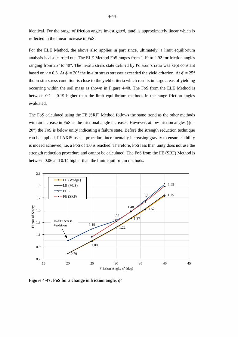
4-44
identical. For the range of friction angles investigated, tanϕ' is approximately linear which is
reflected in the linear increase in FoS.
For the ELE Method, the above also applies in part since, ultimately, a limit equilibrium
analysis is also carried out. The ELE Method FoS ranges from 1.19 to 2.92 for friction angles
ranging from 25° to 40°. The in-situ stress state defined by Poisson’s ratio was kept constant
based on v = 0.3. At ϕ' = 20° the in-situ stress stresses exceeded the yield criterion. At ϕ' = 25°
the in-situ stress condition is close to the yield criteria which results in large areas of yielding
occurring within the soil mass as shown in Figure 4-48. The FoS from the ELE Method is
between 0.1 – 0.19 higher than the limit equilibrium methods in the range friction angles
evaluated.
The FoS calculated using the FE (SRF) Method follows the same trend as the other methods
with an increase in FoS as the frictional angle increases. However, at low friction angles (ϕ' =
20°) the FoS is below unity indicating a failure state. Before the strength reduction technique
can be applied, PLAXIS uses a procedure incrementally increasing gravity to ensure stability
is indeed achieved, i.e. a FoS of 1.0 is reached. Therefore, FoS less than unity does not use the
strength reduction procedure and cannot be calculated. The FoS from the FE (SRF) Method is
between 0.06 and 0.14 higher than the limit equilibrium methods.
Figure 4-47: FoS for a change in friction angle, ϕ'
0.79
1.00
1.22
1.37
1.52
1.75
1.19
1.33
1.48
1.66
1.92
0.7
0.9
1.1
1.3
1.5
1.7
1.9
2.1
15 20 25 30 35 40 45
Fac
tor
of
Saf
ety
Friction Angle, ϕ' (deg)
LE (Wedge)
LE (MoS)
ELE
FE (SRF)
In-situ Stress
Violation

4-45
Figure 4-48: ELE Method yielding zones for friction angle, ϕ' = 25° and v' = 0.3
Cohesion
Figure 4-49 shows the FoS against a change on soil cohesion. As with the friction angle, the
FoS is directly proportional to the cohesion. For the given geometry, the FoS increases by
approximately 0.1 per 5kPa increase in cohesion. The same rate of increase is applicable for
both the limit equilibrium, ELE and FE (SRF) Methods. The difference in FoS stays constant
between the methods: The FoS of the ELE and FE (SRF) Methods are between 0.12-0.15 higher
than the limit equilibrium methods.

4-46
Figure 4-49: FoS for a change in cohesion, c'
Unit weight
The major driving force to instability in a laterally supported excavation is the weight of the
retained soil. Stability of the anchored excavation, with an adequate FoS, is ensured by the
addition of reinforcing. Since the system, without the addition of reinforcing, is not in static
equilibrium – that is, there is a deficit in force/moment resistance – an increase in unit weight
should theoretically further increase this deficit and hence decrease the FoS.
Figure 4-52 shows the impact of a change in soil unit weight, γ, on the FoS. The limit
equilibrium methods, as predicted, show a decline in FoS with an increase in soil unit weight.
The Wedge Method and MoS, which closely follow each other, result in a decrease in the FoS
from 1.83 to 1.36 for a change of unit weight from 16 to 21kN/m3.
The unit weight seems to, however, have a small influence on the FoS of the ELE and FE (SRF)
Methods. The FoS only decreases by 0.04 for a change of unit weight from 16 to 21kN/m3. The
reason for this is twofold:
1. The shape of the critical failure surfaces contributes to the difference between the finite
element and limit equilibrium methods. Figure 4-53 and Figure 4-54 show the failure
mechanisms of the limit equilibrium and finite element methods respectively. The
Wedge Method and MoS both have steep failure mechanisms (~60° above the
horizontal), whereas the ELE and FE (SRF) Methods have deeper failure mechanisms
with flatter rupture planes. Figure 4-50 shows the forces acting on a inclined rupture
1.65
1.46
1.52
1.56
1.66
1.70
1.81
1.58
1.77
1.4
1.45
1.5
1.55
1.6
1.65
1.7
1.75
1.8
1.85
0 2 4 6 8 10 12
Fac
tor
of
Saf
ety
Cohesion, c' (kPa)
LE (Wedge)
LE (MoS)
ELE
FE (SRF)
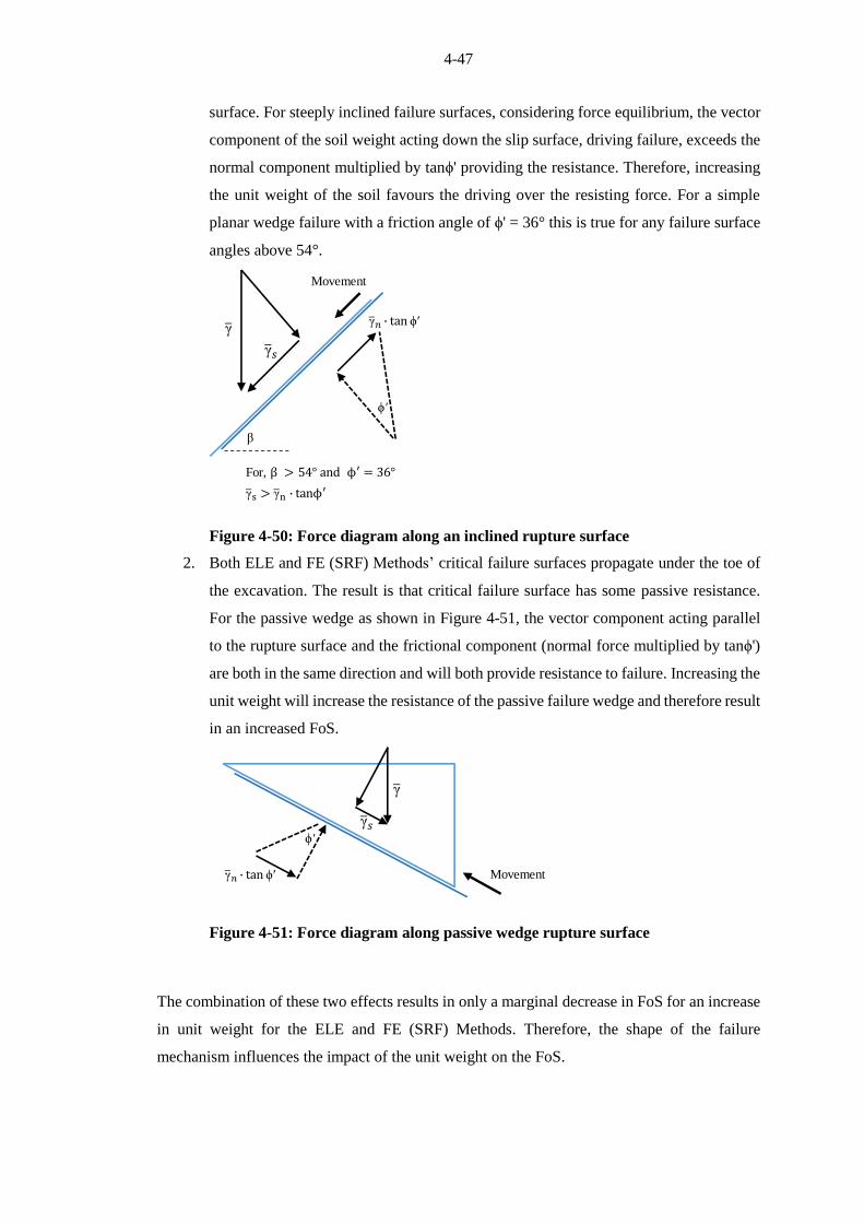
4-47
surface. For steeply inclined failure surfaces, considering force equilibrium, the vector
component of the soil weight acting down the slip surface, driving failure, exceeds the
normal component multiplied by tanϕ' providing the resistance. Therefore, increasing
the unit weight of the soil favours the driving over the resisting force. For a simple
planar wedge failure with a friction angle of ϕ' = 36° this is true for any failure surface
angles above 54°.
Figure 4-50: Force diagram along an inclined rupture surface
2. Both ELE and FE (SRF) Methods’ critical failure surfaces propagate under the toe of
the excavation. The result is that critical failure surface has some passive resistance.
For the passive wedge as shown in Figure 4-51, the vector component acting parallel
to the rupture surface and the frictional component (normal force multiplied by tanϕ')
are both in the same direction and will both provide resistance to failure. Increasing the
unit weight will increase the resistance of the passive failure wedge and therefore result
in an increased FoS.
Figure 4-51: Force diagram along passive wedge rupture surface
The combination of these two effects results in only a marginal decrease in FoS for an increase
in unit weight for the ELE and FE (SRF) Methods. Therefore, the shape of the failure
mechanism influences the impact of the unit weight on the FoS.
ϕ'
β
γ γ 𝑛 tan ϕ
γ 𝑠
For, β 54° an ϕ′ = 36°
γ s γ n tanϕ′
Movement
ϕ'
γ
Movement
γ 𝑠
γ 𝑛 tan ϕ

4-48
Figure 4-52: FoS for a change in unit weight, γ
Figure 4-53: Steep failure surface inclinations (left - Wedge Method ; right - MoS)
Figure 4-54: Deep failure surface inclinations (left - ELE Method ; right - FE (SRF)
Method)
1.83
1.51
1.36
1.86
1.68
1.641.661.62
1.2
1.3
1.4
1.5
1.6
1.7
1.8
1.9
15 16 17 18 19 20 21 22
Fac
tor
of
Saf
ety
Unit Weight, γ (kN/m³)
LE (Wedge)
LE (MoS)
ELE
FE (SRF)
-2
2
6
10
14
18
Ele
vation (m
)
-8
-4
0
4
8
12
16
20
Ele
vat
ion
(m
)

4-49
Young’s modulus
Figure 4-55 shows the change in FoS for a range of Young’s moduli values. As with soil-nails,
the FoS is unaffected by Young’s modulus and Poisson’s ratio for the Wedge Method and MoS.
These parameters are associated with the Hooke’s constitutive relationship for an ideal elastic
material which does not feature in limit equilibrium considerations. However, for comparison
purposes, a constant FoS is shown for a range of Young’s moduli values.
The ELE Method shows a decrease in FoS as the Young’s modulus increases. The FoS
decreases by approximately 0.2 by increasing Young’s modulus from 50MPa to 500MPa.
Young’s modulus does not seem large impact on the FoS of the FE (SRF) Method, deviating
by on 0.02 between the minimum and maximum FoS.
Figure 4-55: FoS for a change in soil Young’s modulus, E'
1.51
1.52
1.73
1.53
1.63
1.65
1.4
1.45
1.5
1.55
1.6
1.65
1.7
1.75
10 100 1000
Fac
tor
of
Saf
ety
Young's Modulus, E' (MPa)
LE (Wedge)
LE (MoS)
ELE
FE (SRF)

4-50
Poisson’s ratio
SIGMA/W, the numerical software for the ELE Method, by default uses Poisson’s ratio to
specify the initial in-situ stresses using the 1-Dimensional compression equation (v' / 1-v' ). The
in-situ stress ratio can also be manually defined. This was done to evaluate the influence of
Poisson’s ratio alone. In this section the in-situ stress ratio was defined as K0 = 0.7 for the ELE
and FE (SRF) Methods.
Figure 4-56 shows the change in FoS for changing Poisson’s ratio from v' = 0.2 to v' = 0.4. As
with Young’s modulus, the limit equilibrium methods remain unaffected by Poisson’s ratio.
The ELE Method shows a decrease in FoS with an increase in Poisson’s ratio. The FE (SRF)
Method shows negligible changes in FoS for a change in the Poisson’s ratio.
Figure 4-56: FoS for a change in Poisson’s Ratio, v' (K0 = 0.7)
1.51
1.52
1.81
1.78
1.74
1.65 1.64 1.64
1.4
1.45
1.5
1.55
1.6
1.65
1.7
1.75
1.8
1.85
0 0.05 0.1 0.15 0.2 0.25 0.3 0.35 0.4 0.45 0.5
Fac
tor
of
Saf
ety
Poisson's Ratio, v' (K0 = 0.7)
LE (Wedge)
LE (MoS)
ELE
FE (SRF)

4-51
In-situ stresses
As mentioned before, the ELE Method (SIGMA/W) uses 1-Dimensional compression equation
(v'/1-v') to calculate the coefficient of lateral earth pressure at-rest. Previously, K0 was kept
constant, however, in this section Poisson’s ratio is kept constant and the in-situ stress ratio, K0,
is varied. Figure 4-57 shows the influence of in-situ stress conditions on the FoS. An increase
in FoS is seen for an increase in initial horizontal stresses.
The FE (SRF) (PLAXIS) uses Jaky’s (1944) equation (1 – sinϕ') to determine the in-situ stresses
independent of Poisson’s ratio. As with the ELE Method, the in-situ stress ratio was manually
defined, and in this case, independent of the friction angle. However, the initial in-situ stresses
has a negligible impact on the FoS. The reason for this is that the SRF does not depend on the
in-situ stresses or the stiffness parameters but only on the strength properties of the soil and
reinforcement. This follows from a detailed discussion of the same conclusion presented for
soil-nails (Section 4.2.10).
Figure 4-57: FoS for a change in in-situ stress ratio, K0 (v' = 0.3)
4.3.6 Effect of anchor length and working load on FoS
In practice, the engineer must specify both the anchor length and working loads for the design
of an anchored lateral support system. These are the main variables for the anchor design and
will have a major impact on the stability of the excavation. A fixed-length of 6m is commonly
used in South African residual soils and was adopted for the analyses. The working load has to
be specified to ensure an adequate FoS. Anchors, however, have ultimate and yield capacities
in excess of the allocated working load. The additional capacity allows for overstressing to
1.51
1.52
1.661.78
1.90
2.10
1.65 1.64 1.64 1.64
1.4
1.5
1.6
1.7
1.8
1.9
2
2.1
2.2
0 0.5 1 1.5 2 2.5
Facto
r of
Safe
ty
In-situ stress ratio, K0 (v' = 0.3)
LE (Wedge)
LE (MoS)
ELE
FE (SRF)
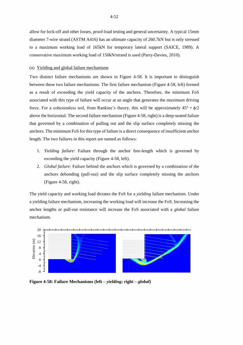
4-52
allow for lock-off and other losses, proof-load testing and general uncertainty. A typical 15mm
diameter 7-wire strand (ASTM A416) has an ultimate capacity of 260.7kN but is only stressed
to a maximum working load of 165kN for temporary lateral support (SAICE, 1989). A
conservative maximum working load of 150kN/strand is used (Parry-Davies, 2010).
Yielding and global failure mechanisms
Two distinct failure mechanisms are shown in Figure 4-58. It is important to distinguish
between these two failure mechanisms. The first failure mechanism (Figure 4-58, left) formed
as a result of exceeding the yield capacity of the anchors. Therefore, the minimum FoS
associated with this type of failure will occur at an angle that generates the maximum driving
force. For a cohesionless soil, from Rankine’s theory, this will be approximately 45° + ϕ/2
above the horizontal. The second failure mechanism (Figure 4-58, right) is a deep-seated failure
that governed by a combination of pulling out and the slip surface completely missing the
anchors. The minimum FoS for this type of failure is a direct consequence of insufficient anchor
length. The two failures in this report are named as follows:
1. Yielding failure: Failure through the anchor free-length which is governed by
exceeding the yield capacity (Figure 4-58, left).
2. Global failure: Failure behind the anchors which is governed by a combination of the
anchors debonding (pull-out) and the slip surface completely missing the anchors
(Figure 4-58, right).
The yield capacity and working load dictates the FoS for a yielding failure mechanism. Under
a yielding failure mechanism, increasing the working load will increase the FoS. Increasing the
anchor lengths or pull-out resistance will increase the FoS associated with a global failure
mechanism.
Figure 4-58: Failure Mechanisms (left – yielding; right – global)
-8
-4
0
4
8
12
16
20
Ele
vat
ion (
m)

4-53
Anchor working load
The influence of increasing the anchor capacity is investigated in this section. In reality there
are some practical limitations when increasing the anchor working load. For example, the
working load has to increase by increments of 150kN which is the design working load per
single strand cable. The capacity cannot be increased by half a strand. However, in this section
the anchor working load is increased by some arbitrary percentage. For all increases/decreases
in working load, the pull-out resistance and yield capacity are increased/decreased
proportionally. To repeat, the following relationships apply to a single strand at 100% working
load:
Working Load = 150kN (SAICE, 1989; Parry-Davies, 2010)
Ultimate Strength = 260.7kN (ASTM A416)
Yield Capacity = 234.6kN (ASTM A416, at 1% elongation)
Unit pull-out resistance = Yield Capacity ÷ Fixed-length = 39.1kN/m
Figure 4-59 shows the change in the FoS for a change in working load for the Wedge Method
and MoS. The failure mechanism at 100% working load, is a steeply inclined failure through
the free-length of the anchors (see Figure 4-53). In other words, as previously discussed, a
yielding type failure occurs. Therefore, an increase in working load results in an increase in
FoS.
Increasing the working load eventually leads to the critical failure mechanisms forming behind
the anchors being favoured. For the MoS, at working load of 125%, a deep-seated global type
failure with a FoS of 1.96, missing most of the anchors, becomes critical. Increasing the
working load beyond 125% has little influence since the failure surface forms behind most of
the anchors. The Wedge Method does not capture this behaviour, as the exit point was fixed at
the toe and additionally curved surfaces from the MoS encourage a failure mechanism to arc
behind the anchors. As long as yielding failure occurs, the Wedge Method and MoS FoS
increases by 0.17 for every 10% increase in working load.
Figure 4-60 shows the change in FoS for a change in working load for the ELE and FE (SRF)
Methods. At 100% working load, the FE (SRF) Method clearly shows a global failure behind
the anchors (see Figure 4-54, right). An increase in working load only results in a minor benefit,
primarily from the bottom anchor, as the slip surface passes around the other anchors. At 80%
of the working load, the critical failure surface passes through the anchor free-lengths and from
this point the FoS rapidly decreases for a decrease in working load. For the ELE Method this
transition occurs at just below 100% of the working load.

4-54
In general, as long as a yielding type failure takes place, it is beneficial to increase the working
load capacity of the anchors i.e. the number of strands in an anchor. Where a global type failure
takes place, increasing the working load (or capacity) will have a small impact.
Figure 4-59: FoS for a change in anchor working load for the Wedge Method and
MoS
Figure 4-60: FoS for a change in anchor working load for ELE and FE (SRF) Methods
1.67
2.46
1.101.23
1.52
1.96 1.97
1
1.2
1.4
1.6
1.8
2
2.2
2.4
2.6
2.8
70% 80% 90% 100% 110% 120% 130% 140% 150%
Fac
tor
of
Saf
ety
Working Load
LE (Wedge)
LE (MoS)
300kN
450kN
600kN
100% Working Load
1.41
1.54
1.66 1.66
1.48
1.61
1.65
1.68
1.3
1.4
1.5
1.6
1.7
1.8
1.9
70% 80% 90% 100% 110% 120% 130% 140% 150%
Fac
tor
of
Saf
ety
Working Load
ELE
FE (SRF)
300kN
450kN
600kN
100% Working Load

4-55
Effect of anchor length on FoS
The effect of changing the anchor length was investigated. The fixed-length was kept constant
at 6m and the free-length of all the anchors was incrementally changed. Figure 4-61 shows the
change in FoS by increasing or decreasing the free-length for different methods of analysis.
Interestingly, no change in FoS is observed for the limit equilibrium methods up to 4m shorter
anchor free-lengths. This is due to the yielding failure mechanism remaining critical. If the
working load were to be increased to 125% (critical point transition discussed in previous
section), reducing the free-length will have an impact on the FoS. This is demonstrated as a
dashed line on Figure 4-61.
The ELE and FE (SRF) Methods closely follow one another with an increase in FoS for an
increase in the anchor free-length. The effect plateaus when increasing the anchor free-length
beyond 2m of the original design length. The observation is a direct opposite occurrence of
increasing the working load previously discussed. An increase in anchor free-length encourages
the failure mechanism to propagate through the free-lengths instead of behind the anchors. By
increasing the free-lengths by 2m, yielding and global failure are simultaneously. This can be
seen in Figure 4-62 showing shadings of incremental shear strain at failure cutting both through
the anchor free-lengths and behind the anchor fixed-lengths. Further increasing the free-lengths
does not render any benefit in terms of FoS.
Figure 4-61: FoS for a change in anchor free-length
1.51
1.52
1.19
1.661.76
1.28
1.801.81
1.96
1
1.2
1.4
1.6
1.8
2
2.2
2.4
-5 -4 -3 -2 -1 0 1 2 3 4 5
Fac
tor
of
Saf
ety
Change in Anchor Free-Length (m)
LE (Wedge) LE (MoS)
ELE FE (SRF)
LE (MoS) @ 125% Working Load
14m
10m
6m
Design Free Lengths
From Figure 4-59

4-56
Figure 4-62: Shadings of incremental shear strain for free-lengths increased by 2m
4.3.7 Effect of surcharge loading on FoS
As with soil-nails, a surface load near the top of the wall might occur that needs to be taken into
account. FHWA (1999) and AASHTO (1996) recommend a surcharge value of approximately
12kPa for excavations in close proximity of roads. Figure 4-63 shows the change in FoS with
an increase in surcharge loading. The effect of surcharge loading is less pronounced than with
the soil-nails as the wall height is twice as high. Therefore, the proportion of surcharge loading
to total loading is less.
The impact of a 15kPa increase in surface contact stress results in a decrease in the FoS of 0.14
for the limit equilibrium methods. The FoS for the ELE Method rapidly declines when applying
a surcharge load. The assumption is made here that the surcharge load is applied throughout the
construction process which negatively impacts the final FoS significantly. If the surcharge load
is only applied on the final loading step, the impact is on the ELE is similar to the FE (SRF)
Method. This is indicated by a dashed line in Figure 4-63.
The FE (SRF) Method FoS only decreases by 0.03 for a 15kPa increase in surcharge. The same
trend in an unresponsive FoS is observed with altering the soil unit weight as discussed in
Section 4.3.5(c). The minor decrease in FoS is due to a deep-seated failure surface being critical.
-10
-5
0
5
10
15
20
-15 -10 -5 0 5 10 15 20 25 30
Ele
vat
ion
(m
)Distance (m)

4-57
Therefore, the vertical stress increase doesn’t significantly increase the driving force. A detailed
discussion is given in Section 4.3.5 (c).
Figure 4-63: FoS for a change surface surcharge loading
4.3.8 Modelling of construction sequence
As with soil-nails, the stability of the excavation needs to be ensured throughout the
construction process. The excavation and installation of a row of anchors can be describing as
follows:
1. Excavation of a horizontal layer to ~0.5m below the anchor position.
2. Installation of the anchor and shotcrete. Anchor post-tensioned to the working load.
3. Repeat step 1, until final level is reached.
During the first excavation phase, the soil is temporarily exposed without any lateral support.
For the remaining excavation phases, the soil near the bottom of the wall is also temporarily
exposed which could result in local instability. In many cases, soldier piles are installed to
beyond the final excavation level prior to excavation taking place. The pile will act as horizontal
beams, supporting the exposed soil. The soil’s undrained behaviour might allow for
unreinforced vertical faces to be stable in the short term. In practice, the site specific conditions
has to be evaluated to assess if the temporary soil strength is sufficient to allow for the
temporary stability. For the purposes in this dissertation, the local stability is not assessed.
1.51
1.38
1.09
1.661.62
1
1.2
1.4
1.6
1.8
2
2.2
0 5 10 15
Fac
tor
of
Saf
ety
Surcharge (kPa)
LE (Wedge)
LE (MoS)
ELE
FE (SRF)
ELE - Final Step

4-58
However, the global stability, given a temporary exposed portion where is the excavation has
taken place, is noted.
Figure 4-64 shows the change in FoS as the construction sequence progresses for the Wedge
Method and MoS. A pair of curves are shown for each method which represent the FoS for the
excavation and anchor installation phases separately. Once the next excavation phase is
advanced the FoS decreases based on the assumption that the material continues to shear in a
drained manner. Immediately after the excavation has taken place, the retained height is
increased but the total reinforcement load remains the same until the next row of anchors are
installed. Another perspective on the same point is that the FoS increases as the installation of
the anchor takes place at a certain depth as shown on Figure 4-64.
The assumption was made that there is some sort of temporary strength (soil or structural) that
will allow for local stability of the soil near the bottom of the wall. The FoS for the initial
excavation has been omitted (FoSwedge = 0.75).
Figure 4-65 shows the change in FoS as a function of excavation depth for the ELE and FE
(SRF) Methods. For comparison, the MoS FoS has been repeated as thin lines in the figure. The
FoS for the ELE Method is comparable to the limit equilibrium methods. Except for the
excavation phase of the FE (SRF) Method, the FoS decreases as the excavation is advanced for
all methods, with the minimum FoS reached at final depth. Whilst the face is temporarily
exposed during the excavation phase, the FE (SRF) Method results in a FoS of approximately
1.3 for all excavation depths. The same trend is seen with soil-nails (Section 4.2.8) and it seems
that for high reinforcement length to height ratios, the FE (SRF) Method results in lower FoS
than other methods. Further research has to be done in this regard.
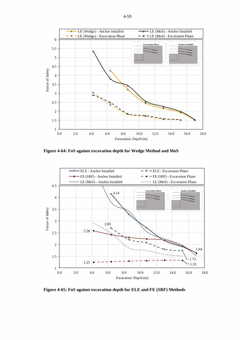
4-59
Figure 4-64: FoS against excavation depth for Wedge Method and MoS
Figure 4-65: FoS against excavation depth for ELE and FE (SRF) Methods
1
1.5
2
2.5
3
3.5
4
4.5
5
5.5
6
0.0 2.0 4.0 6.0 8.0 10.0 12.0 14.0 16.0 18.0
Fac
tor
of
Saf
ety
Excavation Depth (m)
LE (Wedge) - Anchor Installed LE (MoS) - Anchor Installed
LE (Wedge) - Excavation Phase LE (MoS) - Excavation Phase
Anchor InstalledExcavation Phase
4.14
1.64
2.69
1.73
2.58
1.251.33
1
1.5
2
2.5
3
3.5
4
4.5
0.0 2.0 4.0 6.0 8.0 10.0 12.0 14.0 16.0 18.0
Fac
tor
of
Saf
ety
Excavation Depth (m)
ELE - Anchor Installed ELE - Excavation Phase
FE (SRF) - Anchor Installed FE (SRF) - Excavation Phase
LE (MoS) - Anchor Installed LE (MoS) - Excavation Phase
Anchor InstalledExcavation Phase

4-60
4.3.9 Effect of embedded soldier piles
Soldier piles are often installed prior to excavation taking place for anchored lateral support.
The piles are bearing elements distributing the high contact stresses of the anchor head to the
soil. The soldier piles also support the temporary instability created by the excavation prior to
the installation of the anchor and shotcrete. Soldier piles can be embedded to create additional
support below the toe of the excavation.
In this section, the influence of soldier piles is discussed with specific reference to the
embedment depth. Many studies have been done on laterally loaded piles and the mechanism
of failure (Broms, 1965; Wang-Reese, 1986; Poulos, 1989) as discussed in Section 2.1.2.5.
However, the following simplifying assumptions have been made for this study:
For the Wedge Method and MoS, Broms’ (1965) simple relationship for calculating
the pile lateral capacity has been used. Broms tested the lateral passive resistance of
piles by loading at the top of the pile– therefore, ignoring the active force behind the
pile. However, in this section it is assumed that the failure behind the lateral support
extends to the bottom of the soldier pile which includes the active force as shown in
Figure 4-66. The consequence of this assumption is that the retained height is increased
by the depth of the pile.
Figure 4-66: Broms’ theory applied to Wedge Method and MoS
For the ELE and FE (SRF) Methods, due to the limitations of using a plane strain
method of analysis, piles were modelled as 2D plate elements. This means that the piles
act as a wall rather than discrete vertical inclusions.
Piles are adequately designed and do not fail in shearing or bending of the pile. Failure
occurs by passive failure of the soil at the toe. Due to this assumption, embedment
depths of 3m or less below were investigated.
Figure 4-67 shows the pile lateral capacity for a given embedment depth based on Broms’
(1965) theory. The soldier pile lateral resistance is specified as a horizontal point load at the
excavation toe for limit equilibrium methods. At a 3m embedment depth, a soldier pile has
D
Active Force
Passive Force (Broms, 1965)

4-61
almost 600kN of lateral resistance which is equivalent to an additional 4 strand anchor. Note
that the passive resistance was not factored.
Figure 4-68 shows the influence of the embedment depth of the piles on FoS. The pile
embedment depth decreases the FoS for the limit equilibrium methods. The reason for this is
that the active driving force has been extended to the bottom of the embedded pile. For shallow
embedment depths, the increase in active pressure exceeds the passive resistance calculated
using Broms’ theory and hence the FoS decreases. The decrease in FoS with failure depth is
due to the failure mechanism and is further discussed Section 4.4.2.
The ELE Method shows a decrease in FoS as the pile depth is increased. As with soil-nails, the
ELE Method calculates the stability at a working state and the pile capacity is never considered
at failure.
The FE (SRF) Method shows a constant FoS with pile embedment depth. The reason for this is
that even without incorporating piles, the failure surface propagates behind the anchors and
approximately 5m below the wall toe (see Figure 4-58, right). Therefore, including piles with
an embedment depth of up to 3m has no influence on the FoS. If the failure mechanism is forced
to go through the free-lengths by increasing the anchor lengths by 4m (see Figure 4-58, left),
the FoS increases from 1.81 to 1.95 for an 3m embedded soldier pile, which is still substantially
less than the benefit seen in the limit equilibrium methods.
Figure 4-67: The lateral resistance of piles as a function of embedment depth according
to Broms (1965)
26.3
kN
105.4 kN
237.1 kN
0
0.5
1
1.5
2
2.5
3
0 100 200 300 400 500 600 700
Em
bed
men
t D
epth
, D (m
)
Lateral Resistance (kN)
Per Pile
Per Metre (2.5m pile spacing)
• φ' = 36°
• γ= 19kN/m³
• Pile Diameter, b = 600mm
Broms
(1965)

4-62
Figure 4-68: FoS for change in soldier pile embedment depth
1.51
1.34
1.52
1.39
1.34
1.52
1.50
1.641.64
1.3
1.4
1.5
1.6
1.7
1.8
1.9
0 0.5 1 1.5 2 2.5 3 3.5
Facto
r of
Safe
ty
Embedment Depth (m)
LE (Wedge)
LE (MoS)
ELE
FE (SRF)
D

4-63
4.4 DISCUSSION
The results of the analyses have been discussed throughout Chapter 4. This section provides
additional explanations to some of the main observations.
4.4.1 Stress condition violation
In-situ stress specification
The yield criterion for an elastic plastic model is based on the Mohr-Coulomb criterion shown
in Figure 4-69. An in-situ stress state should not be specified as to violate the failure criterion
of the material, i.e. a combination of normal and shear stress plotting above the Mohr-Coulomb
failure envelope.
Figure 4-69: Mohr-circle of stress showing valid, invalid and minimum stress conditions
For a horizontal ground level, the major principal stress is defined by the vertical pressure, σv.
For a cohesionless material, the coefficient of lateral earth pressure in the Rankine active state
can be derived from the ratio of principal stresses and the tangential Mohr-Coulomb failure
envelope. Equation (4.2) shows the classical Mohr-Coulomb failure envelope. Equation (4.3)
shows the coefficient of lateral earth pressure of an active state for a cohesionless soil. The
Rankine active pressure coefficient defines the minimum allowable horizontal stress.
Mohr-Coulomb failure envelope: 𝜏′ = 𝜎′ tan(𝜙′) + 𝑐′ (4.2)
Rankine’s active pressure coefficient: 𝐾𝑎 = 1 − sin𝜙′
1 + sin𝜙′ (4.3)
Shea
r S
tres
s, τ
Normal Stress, σn
Valid in-situ
stress, K0σv
Minimum
horizontal stress
In-situ stress
violation, K0σv
c'
ϕ'
σv = γ ∙ z

4-64
The presence of cohesion will reduce the pressure distribution behind a retained face, i.e. a
reduction in horizontal stress. This can easily be understood from Figure 4-69: An increase in
cohesive strength, c', will elevate the failure envelope, allowing lower values of horizontal
stress to occur at the same vertical stress before yielding occurs.
For a soil with cohesive strength, the minimum horizontal stress can be derived in terms of the
vertical stress and the geometrical constants of the linear Mohr-Coulomb failure envelope as
shown in Equation (4.4).
𝜎ℎ = 𝜎𝑣𝐾𝑎 − 2𝑐′√𝐾𝑎 (4.4)
If a coefficient of lateral earth pressure is specified in any way so that the horizontal stress is
less than minimum allowable horizontal stress shown in Equation (4.4), the entire soil mass
will violate yield in its in-situ state which is not possible. A possible way to make this error, is
to specify the in-situ stress ratio smaller than active pressure using Poisson’s ratio and the 1-
Dimensional compression relationship as shown in Equation (4.5).
1-Dimensional compression: 𝐾0 =𝑣
1 − 𝑣 (4.5)
A cross-section of a propped excavation model using SIGMA/W is shown in Figure 4-70. For
the cohesionless material selected in this analysis, the active pressure coefficient defined by
Equation (4.3) for a material of ϕ' = 40° is less than the in-situ pressure defined by
Equation (4.5). The yellow highlighted zones indicate elements within the model where
yielding has occurred. Yielding generally occurs at a steep angle of approximately 60° above
the horizontal along elements with high shear stress, reflecting the formation of a slip surface
of an active failure wedge.
The impact of violating the in-situ stress conditions is shown in Figure 4-71. Here the in-situ
horizontal stress, defined by the coefficient of lateral earth pressure for 1-Dimensional
compression, is less than the minimum horizontal pressure defined for a material with a friction
angle of ϕ' = 30°, i.e. K0 < Ka. This causes yielding throughout the soil mass which is not
permissible.

4-65
For a cohesionless material the in-situ coefficient of lateral earth pressure has to be greater than
the active horizontal earth pressure coefficient. For an in-situ coefficient defined by the 1-
Dimensional compression equation, the following can be stated:
𝐾𝑎 ≤ 𝐾𝑜
or
1 − sin𝜙′
1 + sin𝜙′ ≤
𝑣
1 − 𝑣 (4.6)
Equation (4.6) can be graphically interpreted as shown in Figure 4-72. The inequality of
Equation (4.6) defines the boundary between permissible in-situ stress conditions and ϕ' – v'
combinations violating the in-situ yield criterion when using the 1-Dimensional compression
equation. PLAXIS (FE (SRF) Method) uses Jaky’s (1944) empirical equation (K0 = 1 – sinϕ')
to define the in-situ stress ratio. As shown in Figure 4-72, Jaky’s equation does not violate the
in-situ stress condition.
Note, that even if the in-situ stresses are not explicitly defined by the user, and a gravity turn-
on procedure is used, the in-situ stresses could still be violated by incorrectly specifying
Poisson’s ratio. If the soil surface is horizontal, the loading is 1-Dimensional since movement
at the sides (left and right) of the numerical model are prevented by a horizontal boundary
condition and movement in-plane is restrained because of the plane strain problem definition.
A modeller should be careful not to specify Poisson’s ratio independently of the friction angle,
or specify the in-situ stresses, K0, in such a way to violate the yield criterion.
Figure 4-70: Cross-section propped excavation showing valid in-situ stresses
• ϕ' = 40° Ka = 0.217
• ' = 0.22 K0 = 0.282
• Ka < K0 Valid model
Yielded Zones
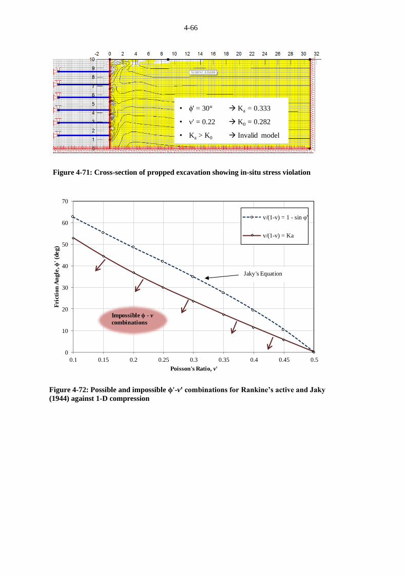
4-66
Figure 4-71: Cross-section of propped excavation showing in-situ stress violation
Figure 4-72: Possible and impossible ϕ'-v' combinations for Rankine’s active and Jaky
(1944) against 1-D compression
• ϕ' = 30° Ka = 0.333
• ' = 0.22 K0 = 0.282
• Ka > K0 Invalid model
0
10
20
30
40
50
60
70
0.1 0.15 0.2 0.25 0.3 0.35 0.4 0.45 0.5
Fri
ctio
n A
ngle
, ϕ' (d
eg)
Poisson's Ratio, v'
v/(1-v) = 1 - sin φ'
v/(1-v) = Ka
Impossible Phi - v combinationsImpossible ϕ - v
combinations
Jaky's Equation

4-67
4.4.2 Failure mechanism
A major drawback to the limit equilibrium and the ELE Methods is that some assumptions must
be made about the shape and position of the failure mechanism. For complex geometries, this
becomes an increasingly difficult task but even for a simple geometry such as a vertical
excavation, there still might be some limitations to assuming a failure surface.
An advantage to using the FE (SRF) Method is being able to determine a failure mechanism
without making any a priori assumptions around shape or position. With the Wedge Method, a
straight line is assumed and the exit point is specified at the toe of the wall. The MoS assumes
a circular failure mode with varying radii as well as entry and exit points. The ELE Method
calculates the stresses on the failure surface using a finite element procedure but still uses the
MoS. With the FE (SRF) Method, deformation takes place in increments as the shear strength
of the soil is reduced by the strength reduction technique. A mechanism ‘naturally’ develops
without any assumptions being made about the position or shape.
Soil-nailed excavation
Figure 4-73 shows shadings of incremental shear strain at failure for the soil-nailed excavation
presented in Section 4.2. Clear bands of shear strain indicate the slip mechanism that has formed
using the FE (SRF) Method. At the exit side of the mechanism, a small passive failure is seen
extending approximately 1m below the toe of the wall. On the entry side of the failure
mechanism, the slip angle steepens near second soil-nail. Neither the planar Wedge Method
(exiting at the toe of the lateral support) nor the MoS or ELE Method (circular slip surfaces)
can capture the shape of the mechanism shown by the FE (SRF) Method adequately.
A multiple wedge method consisting of a double wedge failure behind the lateral support and
a passive resisting wedge can, however, capture the mechanism formed in the FE (SRF)
Method.
SNAIL (SnailWin 3.10) software has been developed by the California department of
Transportation (CALTRANS) to capture a double wedge failure mechanism. Additionally, the
software includes a search for a more critical FoS by including passive wedges below the toe
of the lateral support.
Figure 4-74 shows a compound slip surface for a multiple wedge analysis using SNAIL. A
critical FoS = 1.34 is obtained which is lower than previously calculated for limit equilibrium
methods. Figure 4-75 shows other possible failure mechanisms with their associated FoS. A
planar wedge failure exiting at the toe of the wall has a critical FoS = 1.58, which is the same
as the previous calculations using the Wedge Method. The decrease in FoS seen in a multiple

4-68
wedge analysis is due to a combination of, (a) a double wedge failure and (b) the failure surface
forming below the toe.
a) A double wedge failure, without a passive wedge, results in a marginal decrease in FoS
of 0.04, from 1.58 to 1.54. Refer Figure 4-75.
b) A planar wedge failure, with a passive wedge below the toe, results in a decrease in
FoS of 0.21 from 1.58 to 1.37. Refer Figure 4-75.
Figure 4-73: FE (SRF) Method showing shadings of incremental shear strain at failure
for soil-nailed excavation
Figure 4-74: Multiple wedge analysis critical FoS and compound failure mechanism
-3
-2
-1
0
1
2
3
4
5
6
7
8
9
10
-6 -4 -2 0 2 4 6 8 10 12 14
Ele
vat
ion
(m
)
Distance (m)
FoS = 1.42
-2
0
2
4
6
8
10
-10 -5 0 5 10 15
Ele
vati
on
(m
)
Distance (m)
FoS = 1.34

4-69
Figure 4-75: Various failure mechanisms and FoS including planar, double and passive
wedges
The significant decrease in FoS associated with a passive wedge below the toe is explained
using Rankine’s pressures. Figure 4-76 shows the active, passive and nett (active – passive)
pressures for an 8.5m soil-nailed excavation with a cohesionless soil. For a small increment of
depth below the toe of the wall, the addition of force from the active pressure distribution
exceeds that of the passive pressure. Of course, in reality the pressure distribution will not
resemble the idealistic Rankine pressures, however, it still adequately demonstrates the point:
that for multiple wedges, a failure below the toe of the wall (up to a certain depth) will result in
an increase in nett driving force and hence a decrease in FoS. Furthermore, a wedge failure (at
a given specific angle) that exits below the toe, will be positioned deeper and will have less
reinforcing behind the wedge, decreasing the pull-out resistance and, therefore, decreasing the
FoS.
Generally, for the soil-nailed excavation, it was found that the FE (SRF) Method results in a
lower FoS compared to the limit equilibrium methods. Without varying any parameters, factors
of safety were calculated in Section 4.2 as follows:
Wedge Method: FoS = 1.58
FE (SRF) Method: FoS = 1.42
The reason for the lower FoS from the FE (SRF) Method is a more optimal failure mechanism.
The mechanism includes a bilinear or curved surface with passive failure extending below the
toe of the wall. If a multiple wedge analysis is conducted, the FoS compares well with the FE
(SRF) Method.
-2
0
2
4
6
8
10
-10 -5 0 5 10 15
Ele
vati
on
(m
)
Distance (m)
FoS = 1.54
FoS = 1.58
FoS = 1.37

4-70
Figure 4-76: Rankine's active, passive and net pressure diagrams for soil-nailed
excavation
Anchored excavation
The same phenomenon of failure below the toe of the wall occurs with the anchored excavation.
However, as discussed in Section 4.3, the FoS from the FE (SRF) Method for anchored
excavations is generally higher than limit equilibrium methods which is opposite to the
conclusion for the soil-nailed excavation. Without changing any parameters, the factors of
safety in Section 4.3 as follows:
Wedge Method: FoS = 1.51
MoS: FoS = 1.52
FE (SRF) Method: FoS = 1.64
The reason for this is discovered on closer inspection of the FE (SRF) Method construction
sequence methodology. In the FE (SRF) Method, anchors are pre-stressed to the working load
specified. However, within the material properties of the anchors, in PLAXIS, the yield stress
is also specified. Once a strength reduction technique is applied, soil shear strength properties
are reduced and inevitably the anchors elongate as deformation takes place. The result is an
increased stress within the anchor tendons, eventually mobilising the full yield capacity. The
anchor material is assumed elastic perfectly-plastic which means that once the yield capacity is
reached, the anchor elongates indefinitely ensuring ductility of the structural elements. At
failure, all the anchors have reached their yield capacity. In essence, in previous calculations,
the anchor working loads from the limit equilibrium methods were compared against the anchor
yield capacity of the FE (SRF) Method.
Using the FE (SRF) Method, a decrease in FoS occurs due to failure extending below the toe
while an increase in FoS occurs due the eventual mobilisation of the yield capacity within the
anchors. The combination of these two aspects results in the FE (SRF) Method computing a
FoS of approximately 0.1 higher than the limit equilibrium methods.
-4
-2
0
2
4
6
8
10
-20 -15 -10 -5 0 5 10 15 20D
ep
th (
m)
Distance (m)
Net Pressure
9.5
-200
-150
-100
-50
0
50
100
150
200
250
300
0 1 2 3 4 5 6 7 8 9 10 11 12 13 14 15To
tal
Act
ive
Fo
rce
(kN
pe
r m
wid
th)
Depth below crest @ 8.5m (m)
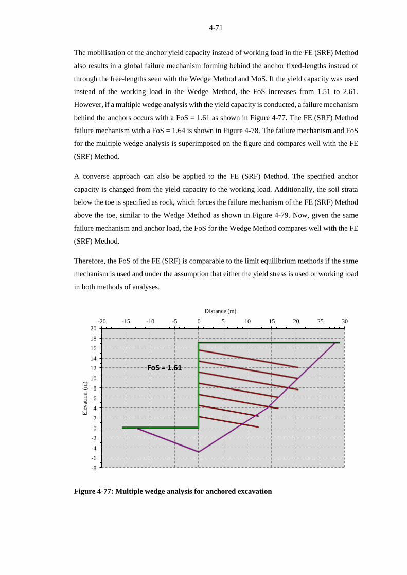
4-71
The mobilisation of the anchor yield capacity instead of working load in the FE (SRF) Method
also results in a global failure mechanism forming behind the anchor fixed-lengths instead of
through the free-lengths seen with the Wedge Method and MoS. If the yield capacity was used
instead of the working load in the Wedge Method, the FoS increases from 1.51 to 2.61.
However, if a multiple wedge analysis with the yield capacity is conducted, a failure mechanism
behind the anchors occurs with a FoS = 1.61 as shown in Figure 4-77. The FE (SRF) Method
failure mechanism with a FoS = 1.64 is shown in Figure 4-78. The failure mechanism and FoS
for the multiple wedge analysis is superimposed on the figure and compares well with the FE
(SRF) Method.
A converse approach can also be applied to the FE (SRF) Method. The specified anchor
capacity is changed from the yield capacity to the working load. Additionally, the soil strata
below the toe is specified as rock, which forces the failure mechanism of the FE (SRF) Method
above the toe, similar to the Wedge Method as shown in Figure 4-79. Now, given the same
failure mechanism and anchor load, the FoS for the Wedge Method compares well with the FE
(SRF) Method.
Therefore, the FoS of the FE (SRF) is comparable to the limit equilibrium methods if the same
mechanism is used and under the assumption that either the yield stress is used or working load
in both methods of analyses.
Figure 4-77: Multiple wedge analysis for anchored excavation
-8
-6
-4
-2
0
2
4
6
8
10
12
14
16
18
20
-20 -15 -10 -5 0 5 10 15 20 25 30
Ele
vat
ion
(m
)
Distance (m)
FoS = 1.61
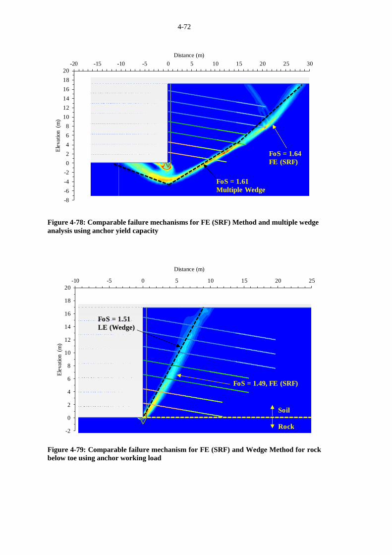
4-72
Figure 4-78: Comparable failure mechanisms for FE (SRF) Method and multiple wedge
analysis using anchor yield capacity
Figure 4-79: Comparable failure mechanism for FE (SRF) and Wedge Method for rock
below toe using anchor working load
-8
-6
-4
-2
0
2
4
6
8
10
12
14
16
18
20
-20 -15 -10 -5 0 5 10 15 20 25 30E
levation (m
)Distance (m)
FoS = 1.61
Multiple Wedge
FoS = 1.64
FE (SRF)
-2
0
2
4
6
8
10
12
14
16
18
20
-10 -5 0 5 10 15 20 25
Ele
vation (m
)
Distance (m)
FoS = 1.49, FE (SRF)
FoS = 1.51
LE (Wedge)
Soil
Rock

4-73
4.4.3 Factors exclusive to FE (SRF) Method
It has been shown that the FE (SRF) Method is comparable to the limit equilibrium methods if
the failure mechanism is consistent across both methods. With anchors, the additional
requirement is that either the anchor’s ultimate capacity or the anchor working load be used
consistently for both methods. These aspects are common to both limit equilibrium and FE
(SRF) methods. However, there are several factors that only apply to the FE (SRF) Method and
not to limit equilibrium methods. It has been shown that some of these factors such as Young’s
modulus, Poisson’s ratio and in-situ stresses have little impact on the FoS calculated from the
FE (SRF) Method (see discussion in Section 4.2.10). There are, however, two factors that
influence the FoS of the FE (SRF) Method which do not appear in limit equilibrium
calculations: angle of dilation and the end bearing effects of the shotcrete facing.
Angle of dilation
For the purposes of the work presented the angle of dilation has been specified as half the
friction angle as discussed in Section 3.2.1. The angle of dilation affects the mobilised friction
angle and therefore the strength of the soil.
Cheng et al. (2007) and Tschuchnigg et al. (2015) have reported that the choice in angle of
dilation makes a small but noticeable difference in stability calculations for slope problems.
Figure 4-80 shows the FoS against dilation angle for the soil-nailed and anchored excavations
using the FE (SRF) Method. The choice of the angle of dilation has an impact on the FoS for
lateral support problems, increasing the FoS by up to 0.08. However, ever there is negligible
change in the calculated FoS when changing the angle of dilation from 18° to 36° (0.5ϕ' to ϕ').
The reason for this is that at such high angles of dilation the soil strength had increased
sufficiently to largely prevent soil yielding.
The FoS could not be calculated for a ψ' = 0 for soil-nails due to a numerical problem. The
mobilisation of soil-nail tension rely in part on the volumetric expansion of the soil in order to
mobilise the tensile capacity within the nails. Using a dilation angle ψ' = 0, causes steep vertical
failures causing instability within the soil-nail model.
PLAXIS (2016) recommends using a dilation angle ψ' = ϕ' - 6° for friction angles greater than
ϕ' = 30°. Figure 4-81 shows the SRF-displacement curve when modelling an excavation using
a low dilation angle of ψ' = 6°. After 400 iterations (the PLAXIS default is 100), 65mm
movement of the face had occurred with the SRF continuously fluctuating and a unique value
could not be defined. Nordal (2008) also reported oscillations in SRF to occur for a non-
associated flow rule in slope stability problems.

4-74
Figure 4-80: FoS against angle of dilation for soil-nailed and anchored excavations for
FE (SRF) Method
Figure 4-81: Movement of lateral support against SRF for soil-nailed excavation using
ψ' = 6°
1.56
1.60
1.64 1.64
1.34
1.381.40 1.41 1.41
1.2
1.3
1.4
1.5
1.6
1.7
0 5 10 15 20 25 30 35 40
Facto
r of
Safe
ty
Angle of Dilation, ψ' (deg)
Anchors - FE (SRF)
Soil-nails - FE (SRF)
0
10
20
30
40
50
60
70
0.9 1.0 1.1 1.2 1.3 1.4
Ho
rizo
nta
l m
ov
emen
t o
f to
p s
oil-n
ail
(mm
)
SRF

4-75
Shotcrete wall end bearing
Extending the shotcrete wall to the toe of the excavation has an influence on the FoS for the FE
(SRF) Method as some end bearing is mobilised below the wall. Stopping the installation of
the shotcrete wall 0.5m above the toe decreases the FoS without altering the failure mechanism.
The FoS decreases by 0.06 to 0.08 as shown in Table 4-5.
Interestingly, if no end bearing is modelled by stopping the shotcrete 0.5m above of the toe,
even closer comparisons in FoS are seen between a multiple wedge analysis and the FE (SRF)
Method. The FoS for the soil-nailed excavation is the same between the two methods of
analysis. The FoS for the anchored excavation differs by only 2%.
Table 4-5: Influence of shotcrete end bearing on FoS for FE (SRF) Method
Model Full shotcrete
End bearing
(SRF)
0.5m above toe
No end bearing
(SRF)
Decrease in
SRF
Multiple
Wedge
Analysis
(FoS)
Soil-Nails, 8.5m 1.42 1.34 0.08 1.34
Anchors, 17m 1.64 1.58 0.06 1.61


CHAPTER 5 CONCLUSIONS AND RECOMMENDATIONS
5.1 CONCLUSIONS
The stability of a uniform slope, soil-nailed- and anchored excavation have been analysed using
limit equilibrium and finite element methods. Various input parameters have been altered and
the influence on stability in terms of FoS has been reported. These variables include soil
properties, model and reinforcement parameters. Conclusions and recommendations from the
results and discussions in the previous chapter are summarised below.
The objective of the study was to investigate and compare finite element methods to limit
equilibrium methods. With regard to the study objective, the following major conclusions can
be made:
The limit equilibrium single trial Wedge Method (Sheahan & Ho, 2003) compares well
with the Method of Slices (Morgenstern-Price, 1965) throughout the analyses.
The ELE Method is a working stress based method which considers the ratio of
available to mobilized shear stress. Stiffness and strength parameters have an influence
on the FoS calculated from this method. The FoS is also highly dependent on the in-
situ stress conditions. The ELE Method compares poorly with limit equilibrium
methods when analysing stability problems with passive reinforce elements such as
soil-nails or embedded piles as the ultimate capacity of the reinforcement is never
considered. The FoS is in the order of 0.1 higher than limit equilibrium methods when
evaluating active anchor reinforcement and a slope stability problem for the geometries
considered.
The FE (SRF) Method finds an optimised failure mechanism as no a priori assumptions
are made regarding the failure mechanism. The FE (SRF) Method FoS is not influenced
by stiffness variables, in-situ stresses or stage construction modelling. When using
elastic perfectly-plastic soil and reinforcement material models, the FoS is only
influenced by the yield criteria of the materials. The FE (SRF) Method is comparable
to limit equilibrium methods if the following two conditions are met:
o The same failure mechanism is evaluated for both methods.
o The capacity of reinforcement is consistently specified in both methods.

5-2
The following minor (not directly related to the objective) conclusions can be made:
When using finite elements, care should be taken when specifying in-situ stress values
so that the active yield criterion is not exceeded. This will result in an in-situ stress
violation of the entire soil mass causing yield throughout. Poisson’s ratio should not be
selected independently of the friction angle when used for the definition of the in-situ
stress state.
The novel method of combining of Embedded Beams and Plates in PLAXIS for the FE
(SRF) Method can be successfully be used to model soil-nails in residual soils. In this
way, pull-out and yielding properties are both captured.
For the FE (SRF) Method, care should be taken to extend the shotcrete face to coincide
with the bottom of the excavation which could increase the FoS.
Selection of the angle of dilation in finite element methods remains problematic. Low
angles of dilation cause numerical instabilities. Increasing the angle of dilation results
in a relatively small but noticeable increase in the FoS.
The ELE Method is sensitive to the properties of the boundary distances and the mesh
resolution.
The FE (SRF) Method appears to be relatively insensitive to the boundary distances or
the mesh resolution.
5.2 RECOMMENDATIONS
When carrying out finite element or limit equilibrium analyses of lateral support, the following
recommendations are made:
Understanding of the finite element procedure can lead to meaningful analyses for soil-
nails and anchors in lateral support. However, due to the complexities and the many
variables of the FE (SRF) Method, the FoS should be cross referenced with a simple
limit equilibrium method as recommended Cheng et al. (2007).
Codes of practice readily address limit equilibrium methods. There is a need for a code
of best practice in the use of finite element methods as suggested by Potts (2003).
The ELE Method should not be used for stability calculations at failure if reinforcement
elements are included.
Traditionally, anchors are checked for internal and external stabilities separately.
FHWA (1999) recommends that a fixed-length will contribute according to the
proportion of it being behind the failure surface. Using this recommendation, slip
surfaces cutting through the free-lengths, through the fixed-lengths and behind the

5-3
fixed-length can be checked in one analysis. By specifying a conservative anchor unit
pull-out resistance, there is no need to separately analyse internal and external
stabilities for automated slip surface searches and SRF methods alike.
Several definitions of FoS exist. Caution should be taken in comparing FoS from
different codes. In general, the SRF is the same as the FoS if the FoS is defined such
that the variability is included in the soil shear strength parameters.


CHAPTER 6 REFERENCES
Adikari, G.S.N. and Cummins, P.J. 1985. An effective stress slope stability analysis method for
dams. Proceedings of the 11th International Conference on Soil Mech and Foundation
Engineering. Vol 2, pp 713-718.
ASTM A416. 1987. Standard specification for uncoated 7-wire stress relieved steel strand for
prestressed concrete. American Society of Testing and Materials, Philadelphia.
Atkinson, J.H. 1993. An Introduction to the Mechanics of Soils and Foundations: Through
Critical State Soil Mechanics. McGraw-Hill, Maindenhead, U.K.
Azzouz, A.S., Baligh, M.M. and Ladd, C.C. 1983. Corrected field vane strength for
embankment design. Journal of Geotechnical Engineering, Vol 109, No 5, pp 730-734.
Babu, G.L.S and Singh, V.K. 2011. Reliability-based load and resistance factors for soil-nail
walls. Canadian Geotechnical Journal, Vol 48, pp 915-930.
Bathe, K.J. 1982. Finite Element Procedures. Prentice Hall.
Bishop, A.W. 1955. The use of the slip circle in the stability analysis of slopes. Geotechnique,
Vol 5, No 1, pp 7-17.
Bjerrum, L. and Landva, A. 1966. Direct simple shear test on a Norwegian quick clay.
Norwegian Geotechnical Institute Publication, No. 070, pp 1-20.
Bjureland, W. 2013. Analysis of deep excavations using the mobilized strength design (MSD)
method. Master Thesis. KTH University, Stockholm.
Brinkgreve, R.B.J. and Bakker, H.L. 1991. Non-linear finite element analysis of safety factors.
Computer methods and advances in geomechanics. Ed. Beer, Booker & Carter. Balkema,
Rotterdam.
Brinkgreve, R.B.J. Engin, E, and Swolf, W. 2010. Plaxis 2D 2010 user manual: Finite Element
code for soil and rock analyses. Plaxis b.v. Netherlands.
Broms, B.B. 1968. Swedish tieback system for sheet pile walls. Proceedings of the 3rd
Budapest Conference on Soil Mechanics and Foundation Engineering, pp 391-403.

6-2
Bolton, M.D. 1986. The strength and dilatancy of sands. Geotechnique, Vol 36, No 1, pp 65-
78.
Bolton, M.D. 1996. Geotechnical design of retaining walls. The Structural Engineer, Vol 74,
No 21, November, pp 365-369.
Bolton, M.D. Powrie, W. and Symons, I.F. 1990a. The design of stiff in-situ walls retaining
over-consolidated clay part 1, short term behavior. Ground Engineering, Vol 23, No 1, pp
34-39.
Bolton, M.D. Powrie, W. and Symons, I.F. 1990b. The design of stiff in-situ walls retaining
over-consolidated clay part 2, short term behaviour. Ground Engineering, Vol 23, No 2,
pp 22-28.
Bowles, J.E. 1996. Foundation analysis and design. 2nd ed. McGraw-Hill, USA.
BS EN 1997-1. 2004. Eurocode 7 Geotechnical Design. British Standards Institution, London.
Bridle, R.J. and Davies, M.C.R. 1997. Analysis of soil nailing using tension and shear:
experiment observations and assessment. Proceedings of the ICE Geotechnical
Engineering, Vol 125, No 3, pp 155-167.
Bruce, D.A. and Jewell, R.A. 1987. Soil Nailing: Application and Practice – 2 Parts, Ground
Engineering, Vol 20, No 1, January, pp 21-28.
BS 4449. 2005. Steel for the reinforcement of concrete. Weldable reinforcing steel. Bar, coil
and decoiled product. Specification. British Standards Institute, London.
BS 8006. 1995. Code of practice of strengthened / reinforced soils and other fills. British
Standards Institute, London.
BS 8081. 1989. Ground Anchorages. British Standards Institute, London.
Franki Africa. 2008. A Guide to Practical Geotechnical Engineering in Southern Africa. 4th ed.
Franki Africa, South Africa.
Calladine, C.R. 1985. Plasticity for engineers. Ellis Horwood, England.
Caquot, A. I. and Kerisel, J. 1948. Tables for the calculation of passive pressure, active pressure,
and bearing capacity of foundations. Translated by M.A. Bec, London. Gauthier-Villars,
Paris

6-3
Chen, W.F. and Liu X.L. 1990. Limit analysis in soil mechanics. Developments in geotechnical
engineering Vol 52. Elsevier Science Publishing Company, New York.
Cheng, Y.M. Lansivaara, T. and Wei, W.B. 2007. Two-dimensional slope stability analysis by
limit equilibrium and strength reduction methods. Computers and Geotechnics. Vol 34,
No 3, pp 137–150.
Cheney, R.S. 1984. Permanent Ground Anchors. Publication Report FHWA-DP-68-1R.
Federal Highway Administration, Washington D.C.
CIRIA. 2005. Soil Nailing Best Practice Guide. Report C637. CIRIA Publications, London.
Clayton, C.R.I. Woods, R.I. Bond, A.J. and Milititsky J. 2013. Earth Pressure and Earth-
Retaining Structures. 3rd ed. CRC Press (Taylor & Francis Group), Flordia, USA.
Clough, R.W. and Woodward, R.J. 1967. Analysis of embankment stresses and deformations.
Journal of Soil Mechanics and Foundation Engineering, ASCE. Vol 93, pp 529-544.
Clouterre. 1991. French National Research Project Clouterre (English Translation, 1993) –
Federal Highways Administration FHWA-SA-93-026. FHWA, Washington, USA.
Committee of Inquiry (COI). 2005. Committee of Inquiry into the Incident at the MRT Circle
Line Worksite that led to the Collapse of Nicoll Highway on 20 April 2004. Ed. Magnus,
Teh, Lau. Singapore Government Ministry of Manpower, Singapore.
Coulomb, C.A. 1773. Essai sur une application des re`gles de maximis & minimis a` quelques
proble`mes de statique, relatifs a l’architecture. Me´m. Math. Phys. Acad. R. Sci. Vol 7, pp
343–382. English translation: Note on an application of the rules of maximum and
minimum to some statical problems, relevant to architecture. In Heyman, J. 1972.
Coulomb’s memoir on statics: An essay on the history of civil engineering. Cambridge
University Press, Cambridge, UK.
Craig, R.F. 2004. Craig’s Soil Mechanics. 7th ed. Spon Press, New York.
Das, B.M. 1999. Principles of foundation engineering. 4th ed. PWS Publishers, Pacific Grove,
California, pp 862.
Dawson, E.M. Roth, W.H. and Drescher, A.A. 1999. Slope stability analysis by strength
reduction. Geotechnique, Vol 49, No 6, pp 835–840.
Day, P.W. 2013. Site Investigation Codes & Standards, Power Point Presentation File. Site
Investigation Course, SAICE Geotechnical Division.

6-4
Drucker, D.C. and Prager, W. 1952. Soil mechanics and plastic analysis in limit design.
Quarterly of Applied Mathematics, Vol 10 No 2, pp 157-165.
Duncan, J.M. 1996. State of the art: Limit equilibrium and finite-element analysis of slopes.
Journal of Geotechnical Engineering, Vol 122, pp 577–596.
Elias, V. and Juran, I. 1991. Soil Nailing for Stabilization of Highway Slopes and Excavations.
Publication FHWA-RD-89-198, Federal Highway Administration, Washington D.C.
Fan, C. C. and Luo, J. H. 2008. Numerical study on the optimum layout of soil nailed slopes.
Computers and Geotechnics. Vol 35, No 4, pp 585-599.
Fang, H.Y. 1991. Foundation Engineering Handbook. 2nd ed. Van Nostrand, New York.
Farias, M.M. and Naylor, D.J. 1996. Safety analysis using finite elements. Infogeo 96, Sao
Paulo, Brazil.
Fellenius, W. 1936. Calculation of the stability of earth dams. Proceedings of the 2nd Congress
on Large Dams, Vol 4, pp 445.
FHWA. 1988. Permanent Ground Anchors. Federal Highway Administration Report FHWA-
DP-68-1R. FHWA, Washington, D.C
FHWA. 1998. Manual for Design and Construction Monitoring of Soil Nail Walls. Federal
Highway Administration Report FHWA-SA-96-069R. FHWA, Washington, D.C.
FHWA. 1999. Geotechnical Engineering Circular No. 4 – Ground Anchors and Anchored
Systems. Federal Highway Administration Report FHWA-IF-99-015. FHWA,
Washington, D.C.
FHWA. 2003. Geotechnical Engineering Circular No. 7 Soil Nail Walls. Federal Highway
Administration Report FHWA0-IF-03-017. FHWA, Washington, D.C.
Fredlund, D.G. and Krahn, J. 1977. Comparison of slope stability methods of analysis.
Canadian Geotechnical Journal, Vol 14, No 3, pp 429-439.
Fredlund, D.G. and Scoular, R.E.G. 1999. Using limit equilibrium concepts in finite element
slope stability analysis. Proceedings of the International Symposium on Slope Stability
Engineering. Ed Yagi, Yamagami & Jiang. Balkema, Rotterdam, pp 31-47.
Gässler, G. 1988. Soil-nailing. Theoretical basis and practical design. Proceedings of the
International Geotechnical Symposium on Theory and Practice of Earth Reinforcement,
Balkema, Japan, pp 283-285.

6-5
Gässler, G. and Gudehus, G. 1981. Soil nailing – some aspects of a new technique. Proceedings
of the International Conference on Soil Mechanics and Foundation Engineering,
Stockholm, Sweden.
Gens, A. 2012. PLAXIS Advanced Course on Computational Geomechanics, Hong Kong.
GeoStudio Version 2007. Geo-Slope International, Calgary, Canada.
Griffiths, D.V. 1982. Computation of bearing capacity factors using finite elements.
Geotechnique, Vol 32, No 3, pp 195-202.
Griffiths, D.V. and Lane, P.A. 1999. Slope stability analysis by finite elements. Geotechnique,
Vol 49, No 3, pp 387–403.
Gunaratne, M. 2014. The Foundation Engineering Handbook. 2nd ed. CRC Press (Taylor &
Francis Group), Florida, USA.
Harr, M.E. 1977. Mechanics of Particulate Media: A Probabilistic Approach. McGraw-Hill,
New York.
Heyman, J. 1973. The stability of a vertical cut. International Journal of Mechanical Science,
Vol 15, pp 845-854.
Heymann, G. 1993. Soil Nailing Systems as Lateral Support for Surface Excavations. Master
Thesis. University of Pretoria.
Heymann, G. Rhode, A.W. Schwartz, K. and Friedlaender, E. 1992. Soil nail pull-out resistance
in residual soils. Proceedings of the International Symposium on Earth Reinforcement
Practice, Kyushu, Japan. Vol 1 pp 487-492.
Highway Agency (HA). 1994. Design methods for the reinforcement of highway slopes by
reinforced soil and soil nailing techniques. HA68/94. HMSO Publications, UK.
Hill, R. 1950. The Mathematical Theory of Plasticity. Clarendon Press, Oxford.
Ingold, T.S. 1995. The practice of soil reinforcing in Europe. Thomas Telford, London.
Institute of Civil Engineers (ICE). 2012. ICE manual of geotechnical engineering Vol 1 and 2.
Ed. Burland, Chapman, Skinner and Brown. ICE Publishing, UK.
Jaky, J. 1944. The coefficient of earth pressure at-rest. Journal of the Geotechnical Engineering
Division of ASCE, Vol 111, No 3, pp 302-318.

6-6
Janbu, N. 1954. Application of composite slip surface for stability analysis. Proceedings of the
European conference on stability of earth slopes, Stockholm, Sweden Vol 3, pp 43-49.
Jewell, R.A. 1980. Some effects of reinforcement on the mechanical behaviour of soils. PhD
Thesis. Cambridge University.
Jewell, R.A. and Pedley, M.J. 1990. Soil nailing design: the role of bending stiffness. Ground
Engineering, Vol 23, No 2, pp 30-36.
Jewell, R.A and Pedley, M.J. 1992. Analysis for soil reinforcement with bending stiffness.
Journal of Geotechnical Engineering Division of ASCE, Vol 118, No 10, pp 1505-1528.
Jewell, R.A. and Wroth, C.P. 1987. Direct shear tests on reinforced sand. Geotechnique, Vol
37, No 1, pp 53-68.
Jones, C.P.D. 1990. In-situ techniques for reinforced soil. Proceedings of the international
reinforced soil conference, Glasgow, pp. 277-282.
Jorge, G.R. 1969. The regroutable IRP anchorage for soft soils, low capacity or karstic rocks.
Proceedings of the 7th International Conference on Soil mechanics and Foundation
Engineering, Speciality Session No 14 and 15, pp 159-163.
Kirsten, H.A.D. 1992. Limit Equilibrium, closed-form elastic, and numerical plastic analyses
of stability of earth wall reinforced with grouted rebar nails and cable anchors. Canadian
Geotechnical Journal, Vol 29, pp 288-298.
Krahn, J. 2003. The 2001 R.M. Hardy Lecture: The limits of limit equilibrium analyses.
Canadian Geotechnical Journal, Vol 40, pp 643-660.
Kranz, E. 1953. Uber die Verankerung von Spundwanden. Wilhelm Ernst & Sohn, Berlin.
Kulhawy, F.H. 1969. Finite element analysis of the behaviour of embankments. PhD Thesis.
The University of California at Berkeley.
Lai Sang, J. and Scheele, F. 1999. Experimental and numerical investigation of soil-nailed wall
structures. Geotechnics for Developing Africa. Ed Wardle, Blight & Fourie. Balkema,
Rotterdam, pp 177-182.
Lin, H. Xiong, W. and Cao, P. 2013. Stability of soil nailed slope using strength reduction
method. European Journal of Environmental and Civil Engineering, Vol 17, No 9, pp 872-
885.

6-7
Littlejohn, G.S. 1990. Ground Anchorage Practice. Proceedings of the Conference on Design
and Performance of Earth Retaining Structures. ASCE, New York, pp 692-733.
McGown, A. Murray, R.T. and Andrawes, K.Z. 1987. Influence of wall yielding on lateral
stresses in unreinforced and reinforced fills. Research Report 113, TRRL, U.K.
Mitchell, J. K. and Villet, W. C. B. 1987. Reinforcement of Earth Slopes and Embankments,
Transportation Research Board, National Co-operative Highway Research Program
Report 290. National Research Council, Washington DC.
Morgenstern, N.R. and Price, V.E. 1965. The analysis of the stability of general slip surfaces.
Geotechnique, Vol 15, No 1, pp 79-93.
Morgenstern, N.R. and Sangrey, D.A. 1978. Methods of stability analysis, Chapter 7. In
Landslides — Analysis and Control. National Academy of Sciences, Washington D.C.,
Special Report 176.
Mollahasani, A. 2015. Application of Submerged Grouted Anchors in Sheet Pile Quay Walls.
PhD Thesis. University of Bologna.
Naylor, D.J. 1982. Finite elements and slope stability. In Numerical methods in geomechanics.
D. Reidel Publishing Company, Holland.
Nordal, S. 2008. Can we trust numerical collapse load simulations using non-associated flow
rules? In Geomechanics in the emerging social and technological age: Proceedings of the
12th IACMAG conference, Goa, India (ed. P. N. Singh), pp. 755–762.
Osman, A.S. and Bolton, M.D. 2004. A new design method for retaining walls in clay.
Canadian Geotechnical Journal, Vol 41, No 3, 453-469.
Osman, A.S. and Bolton, M.D. 2005. Ground movement predictions for braced excavations in
clay. ASCE Journal of Geotechnical and Geoenvironmental Engineering. Vol 132, No 4,
pp 465-477.
Osman A.S. and Bolton M.D. 2006. Design of braced excavations to limit ground movements.
Proceedings of Institution of Civil Engineers, Geotechnical Engineering, Vol 159, No 3,
pp 167-175.
Ostermayer, M. and Scheele, F. 1977. Research on ground anchors in non-cohesive soils.
Proceedings of the 9th International Conference on Soil Mechanics and Foundation
Engineering, Tokyo.

6-8
Owen, D.R.J. and Hinton, E. 1982. Finite Elements in Plasticity. Pineridge Press Ltd, Swansea.
Parry-Davies, R. 2010. A personal account of the history of ground anchors in Southern Africa
including some practical guidance on the subject. SAICE, South Africa.
Pastor, J. and Turgeman, S. 1976. Mise en oeuvre numerique des methodes de l’analyse limite
pour les materiaux de von Mises et de Coulomb standards en deformation plane. Mech.
Res. Commun. Vol 3, No 6, pp 469-476 (in French).
Peck, R.B. 1969. Deep Excavations and Tunneling in Soft Ground, State of Art Report.
Proceedings of the 7th International Conference on Soil Mechanics and Foundation
Engineering, Mexico City, Mexico, pp 225-290.
Pedley, M.J. Jewell, R.A. and Milligan, G. E.W. 1990. A large scale experimental study of
soil-reinforced interaction. Ground Engineering, July/Aug., pp 44-50, and Ground
Engineering, September, pp 46-49.
PLAXIS 2D Version 2016. Plaxis bv, Delft, Netherlands.
PLAXIS. 2016. User’s manual of PLAXIS. Balkema, Netherlands.
Pfister, P. Evens, G. Guilland, M. and Davidson, R. 1982. Permanent Ground Anchors:
Soletanche Design Criteria. Federal Highway Administration Report No FHWA-RD-81-
150. FHWA, Washington D.C.
Post-tensioning institute (PTI). 1980. Recommendations for Prestressed Rock and Soil
Anchors. PTI, Phoenix, Arizona, pp 57.
Potts, D. M. 2003. 42nd Rankine Lecture: Numerical analysis: a virtual dream or practical
reality? Geotechnique, Vol 53, No 6, pp 535-572.
Prager, W. and Hodge, O.G. 1951. Theory of perfectly plastic solids. John Wiley and Sons,
New York.
Rankine, W.J.M. 1857. On the Stability of Loose Earth. Philosophical Transactions of the
Royal Society. London, Vol 147.
Rowe, P. W. 1962. The stress dilatancy relation for static equilibrium of an assembly of
particles in contact. Proceedings of the Royal Society. London, Series A, Vol 269, pp 500-
527.
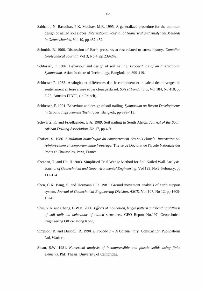
6-9
Sabhahit, N. Basudhar, P.K. Madhav, M.R. 1995. A generalized procedure for the optimum
design of nailed soil slopes. International Journal of Numerical and Analytical Methods
in Geomechanics, Vol 19, pp 437-452.
Schmidt, B. 1966. Discussion of Earth pressures at-rest related to stress history. Canadian
Geotechnical Journal, Vol 3, No 4, pp 239-242.
Schlosser, F. 1982. Behaviour and design of soil nailing. Proceedings of an International
Symposium. Asian Institute of Technology, Bangkok, pp 399-419.
Schlosser F. 1983. Analogies et différences dan le component et le calcul des ouvrages de
soutènement en terre armée et par clouage du sol. Sols et Fondations, Vol 184, No 418, pp
8-23, Annales ITBTP, (in French).
Schlosser, F. 1991. Behaviour and design of soil-nailing. Symposium on Recent Developments
in Ground Improvement Techniques, Bangkok, pp 399-413.
Schwartz, K. and Friedlaender, E.A. 1989. Soil nailing in South Africa, Journal of the South
African Drilling Association, No 17, pp 4-9.
Shafiee, S. 1986. Simulation nume´rique du comportement des sols cloue´s. Interaction sol
reinforcement et comportementde l’ouvrage. The`se de Doctorat de l’Ecole Nationale des
Ponts et Chausse´es, Paris, France.
Sheahan, T. and Ho, H. 2003. Simplified Trial Wedge Method for Soil Nailed Wall Analysis.
Journal of Geotechnical and Geoenvironmental Engineering. Vol 129, No 2, February, pp
117-124.
Shen, C.K. Bang, S. and Hermann L.R. 1981. Ground movement analysis of earth support
system. Journal of Geotechnical Engineering Division, ASCE. Vol 107, No 12, pp 1609-
1624.
Shiu, Y.K. and Chang, G.W.K. 2006. Effects of inclination, length pattern and bending stiffness
of soil nails on behaviour of nailed structures. GEO Report No.197. Geotechnical
Engineering Office. Hong Kong.
Simpson, B. and Driscoll, R. 1998. Eurocode 7 – A Commentary. Construction Publications
Ltd, Watford.
Sloan, S.W. 1981. Numerical analysis of incompressible and plastic solids using finite
elements. PhD Thesis. University of Cambridge.

6-10
Sloan, S.W. 2013. 51st Rankine Lecture: Geotechnical stability analysis. Geotechnique, Vol
63, No 7, pp 531-572.
Sloan, S.W. & Randolph, M.F. 1982. Numerical prediction of collapse loads using finite
element methods. International Journal of Numerical and Analytical Methods in
Geotechnics. Vol 6, No 1, pp 47-76.
Sokolovskii, V.V. 1965. Statics of granular media. Pergamon, New York.
South African Institute of Civil Engineers (SAICE). 1989. Lateral Support in Surface
Excavations – Code of Practice. SAICE, Geotechnical Division, South Africa.
Spencer, E. 1967. A method of analysis of the stability of embankments assuming parallel
interslice forces. Geotechnique, Vol 17, No 1, pp 11-26.
Stocker, M.F. Korber, G.W. Gassler, G. and Gudehus, G. 1979. Soil nailing. Proceedings of
the International Conference on Soil Reinforcement. Vol 2, pp 469-474.
Su, L.J. 2006. Laboratory pull-out testing study on soil nails in compacted completely
decomposed granite fill. PhD Thesis. The Hong Kong Polytechnic University.
Tan, S.A. Lou, S.Q. and Yong, K.Y. 2000. Simplified models for soil-nail lateral interaction.
Ground Improvement, Vol 4, pp 141-152.
Terzaghi, K. 1943. Theoretical Soil Mechanics. John Wiley & Sons, New York.
Terzaghi, K. and Peck, R.G. 1967. Soil Mechanics in Engineering Practice. John Wiley & Sons,
New York.
Tschuchnigg, F. Schweiger, H.F. Sloan, S.W. Lyamin, A.V. and Raissakis, I. 2015.
Comparison of finite-element limit analysis and strength reduction techniques.
Geotechnique, Vol 65, No 4, pp 249–257.
Verruijt, A. 2001. Soil Mechanics. Delft University of Technology, Netherlands.
Vesic, A.S. 1973. Analysis of ultimate loads of shallow foundations. Journal of the Soil
Mechanics and Foundations Division, ASCE, Vol 99, pp 45-73.
Wang, S-T. and Reese, L.C. (1986). Study of Design Methods for Vertical Drilled Shaft
Retaining Walls. Texas State Department of Highways and Public Transportation, Austin,
Texas.

6-11
Zienkiewicz, O.C. Humpheson, C. and Lewis, R.W. 1975. Associated and non-associated
visco-plasticity and plasticity in soil mechanics. Geotechnique, Vol 25, No 4, pp 671-689.
Zhou, W-H. and Yin, J-H. 2008. A simple mathematical model for soil nail and soil interaction
analysis. Computers and Geotechnics, Vol 35, pp 479-488.