finite-wavelength scattering of incident vorticity and...

J. Fluid Mech. (2008), vol. 612, pp. 407–438. c© 2008 Cambridge University Press

doi:10.1017/S0022112008003212 Printed in the United Kingdom

407

Finite-wavelength scattering of incidentvorticity and acoustic waves at a

shrouded-jet exit

A R N A B S A M A N T A1 AND J O N A T H A N B. F R E U N D1,2

1Department of Mechanical Science and Engineering, University of Illinois at Urbana–Champaign,Urbana, IL 61801, USA

2Department of Aerospace Engineering, University of Illinois at Urbana–Champaign, Urbana,IL 61801, USA

(Received 21 December 2007 and in revised form 24 June 2008)

As the vortical disturbances of a shrouded jet pass the sharp edge of the shroudexit some of the energy is scattered into acoustic waves. Scattering into upstream-propagating acoustic modes is a potential mechanism for closing the resonanceloop in the ‘howling’ resonances that have been observed in various shrouded jetconfigurations over the years. A model is developed for this interaction at the shroudexit. The jet is represented as a uniform flow separated by a cylindrical vortexsheet from a concentric co-flow within the cylindrical shroud. A second vortex sheetseparates the co-flow from an ambient flow outside the shroud, downstream of itsexit. The Wiener–Hopf technique is used to compute reflectivities at the shroud exit.For some conditions it appears that the reflection of finite-wavelength hydrodynamicvorticity modes on the vortex sheet defining the jet could be sufficient to reinforce theshroud acoustic modes to facilitate resonance. The analysis also gives the reflectivitiesfor the shroud acoustic modes, which would also be important in establishingresonance conditions. Interestingly, it is also predicted that the shroud exit canbe ‘transparent’ for ranges of Mach numbers, with no reflection into any upstream-propagating acoustic mode. This is phenomenologically consistent with observationsthat indicate a peculiar sensitivity of resonances of this kind to, say, jet Mach number.

1. Introduction1.1. Resonances in shrouded jets

The potential for shrouded jets, or jets fitted with an ejector (see figure 1), to resonatemaking high-intensity discrete-frequency sound was first reported almost forty yearsago by Bradshaw, Flintoff & Middleton (1968) and was called howling. Seeminglysimilar resonances have also been observed in full-scale turbojet engine test cells (seeJones & Lazalier 1992; Sebourn & Shope 2005; Massey et al. 1994). Here, intensetonal pressure fluctuations were observed in the shroud near its inflow end with theresonance frequency closely matching the first asymmetric acoustic modes expected inthe shroud: the so-called (m, n) = (1, 1) mode, where m and n correspond respectivelyto the azimuthal and radial wavenumbers.

How these resonances are sustained inside the shroud is not fully understood. Itis expected that for high amplitudes the acoustic modes can excite the jet instabilitymode by perturbing the jet at the nozzle. Generally, jets are receptive to such

408 A. Samanta and J. B. Freund

Shroud

Nozzle

Jet

L

Ro

Ri

M1, T1

M2, T2

Figure 1. Schematic of a shrouded jet reported to howl.

excitations at the nozzle lip and the resulting instabilities should grow by extractingenergy from the jet at their respective frequencies. It is uncertain, however, howthese flow instabilities generate pressure fluctuations to reinforce the shroud acousticmodes and thereby close the feedback loop. There are several theories for this,including the one that depends upon jet shock cells, described by Tam, Ahuja &Jones (1994). But strong resonances have also been observed for subsonic jets. Forexample, Bradshaw et al. (1968) report subsonic confined jets that for ranges of Machnumbers resonate with tones 20 dB above the corresponding non-resonating spectrumof the jet. Consequently, they speculated that the instability (vorticity) waves supportedby the inner shear layer interact with the nozzle shroud in a way that reflects waveswith pressure fluctuations matching the frequencies of the shroud acoustic modes.This mechanism for closing the feedback loop was included by Howe (1987) in hisanalysis under the assumption that the shroud exit is effectively at a constant pressure.This is a long-wavelength assumption. In actual situations, however, the wavelengthof the sound in the resonance modes is usually comparable to the shroud length,which in turn is comparable to its diameter (e.g. Jones & Lazalier 1992; Sebourn &Shope 2005). It is well known that for open-exit configurations, reflections of out-going acoustic waves are significantly reduced when these lengths are comparable(e.g. Levine & Schwinger 1948).

In this paper, we analyse the acoustic reflection of finite-wavelength vorticaldisturbances with the goal of illuminating the role of vortical flow disturbancesin sustaining shroud resonances of the kind discussed. The model geometry weanalyse is shown in figure 2. It consists of a semi-infinite cylindrical shroud with aco-flowing inner jet issuing out of it. The uniform inner, outer and ambient flows areseparated by vortex sheets, with the outer vortex sheet originating at the shroud exit.The Wiener–Hopf method is used to calculate how vorticity waves on the inner shearlayer scatter at the shroud exit into acoustic waves. Those reflected back upstream intothe shroud have the potential to close the feedback loop. Although the main focus ofthis work remains the incident vorticity modes, the reflectivities of finite-wavelengthoutgoing acoustic modes are obtained with little extra effort. These are reported bothfor completeness and because their reflection is also important for any acousticallycoupled resonance that might occur.

1.2. Analysis as a Wiener–Hopf problem

Acoustic wave reflection from a sharp-ended duct without mean flow was first solvedby Levine & Schwinger (1948) using the Wiener–Hopf method (see Noble 1988). Theyobtained analytical expressions for sound waves radiated and reflected from the open

Scattering of vorticity and acoustic waves at a shrouded-jet exit 409

end of the duct. Mean flow was first included by Carrier (1956), whose analysis wasconsistent with taking Lorentz transformation of the no-flow case in a way that yieldssolutions both for flow into the duct, which makes the duct-lip singularity integrable,and for flow out of the duct, where the Kutta condition is automatically satisfiedfor this solution method. Later, Homicz & Lordi (1975) seem to have rediscoveredthis technique. However, for the exhaust case, a vortex sheet appears at the trailingedge, which needs to be included in the analysis. Mani (1973) derived a solution forthe two-dimensional case with a velocity discontinuity that was extended by Savkar(1975) to a cylindrical geometry. However, none of these solutions included instabilitywaves, since their correct mathematical treatment remained unclear, nor do theycontain any proper treatment of the Kutta condition.

Morgan (1974) and Crighton & Leppington (1974) independently concluded thatwhen a vortex sheet is shed from a semi-infinite plate the Kelvin–Helmholtz instabilitywave must couple to the acoustic field. They recognized that ignoring this waveyields a fundamentally incorrect field and developed procedures for its inclusion.The difficulty in identifying the correct Kutta condition formulation at the duct exithas been explained by Orszag & Crow (1970) and Crighton (1972a, b). The currentaccepted practice is to use the full Kutta condition (Crighton & Leppington 1974),which has experimental support (Bechert & Pfizenmaier 1975).

Munt (1977) was the first to combine all these related theoretical developments toconstruct a complete analytical solution for the transmitted waves for a subsonic jetissuing out of a semi-infinite cylindrical duct. His analysis placed no restriction onthe velocities of the uniform subsonic jet or the co-flow, separated by a cylindricalvortex sheet, and also accounted for density and temperature jumps across the vortexsheet. Excellent agreement was obtained with the measurements of far-field directivity(Pinker & Bryce 1976) and reflection coefficients (see Munt 1990). The near-fieldfeatures of Munt’s results were confirmed by Howe (1979) using different analyticalmethods.

Using Munt’s framework, the problem of a semi-infinite duct with an infinitecentrebody in a uniform mean flow was first considered by Rienstra (1984). This wasrecently extended by Gabard & Astley (2006) to have different velocities inside andoutside the duct with the consequence that instability waves had to be accounted forin the complete solution. Though the flow with a centrebody rather than a jet is, ofcourse, significantly different from the present configuration, we use similar techniqueshere. Taylor, Crighton & Cargill (1993) analysed the same basic configuration as wedo here (figure 2), but only for plane waves in the long-wavelength limit. Insteadof solving the full Wiener–Hopf problem they solved two subproblems: first, soundtransmission from a cylindrical nozzle into an infinite outer cylindrical duct; andsecond, sound transmission from a semi-infinite cylindrical duct containing a co-flow.These two problems were then matched by using plane-wave coupling. We use asimilar two-part approach to generate the incident vorticity wave. These methodshave also been applied to rotating flows (Heaton & Peake 2005). Uniform mean flowis, however, sufficient for studying the phenomena of present interest.

Recent works by Veitch & Peake (2007) and Demir & Rienstra (2007) haveconsidered the far-field sound from the configuration of figure 1 by solving the fullproblem using a matrix Wiener–Hopf technique (details in Veitch & Peake 2008). Thesepapers make an important advance in developing techniques to factor matrix Wiener–Hopf kernels. In the present work we focus entirely on near-field interactions, whereour scalar approach seems more appropriate since it allows us to separately considerdifferent incident wave solutions and explicitly compute their individual interactions


Outer wall

r

z

v3

v2

v1

Ri

Ro

Jet

Co-flow

Ambient flow

Incident wave

Reflected wave

Vortex sheets

Figure 2. Schematic of the shroud with co-flow.

at the shroud exit. Of course, the full solution provided by matrix Wiener–Hopftechniques contains these interactions, but it would seem to require significantly morework to extract the individual interactions of interest. Even after solving the problemby the matrix approach, Veitch & Peake (2008) employ a scalar approach to identifyhow specific interactions contribute to the far-field sound. Obviously, interaction withthe inner nozzle lip, not considered here, becomes important in determining the actualresonance conditions inside the shroud. We prefer to solve that particular problem bysplitting the configuration of figure 1 into two subproblems, as done by Taylor et al.(1993) in the long-wavelength limit, which clarifies the physical picture better.

Extension to finite frequencies and vortical waves is essential for the kind ofinteraction that we consider. The behaviour of the vorticity wave passing the shroudedge in the short-wavelength limit is clear. Since the pressure disturbances associatedwith subsonic vortex sheet modes decay exponentially away from the sheet, forvanishingly short-wavelength there is no interaction between the vortex sheet modesand the shroud exit and thus no reflection. In the long-wavelength limit, such as theone considered by Taylor et al. (1993) for incident acoustic modes, the only reflectedacoustic mode that the system can support is the plane wave, or more precisely aquasi-plane wave, since a true plane wave is impossible to define for multiple streamsinside a duct. Our investigation of the observed asymmetric-mode resonances requiresinclusion of modes that only propagate for finite frequencies. In this study, we alsospecifically focus on the scattering of the vorticity wave into acoustic modes, whichhas not been systematically studied before.

The organization of the paper is as follows. The governing differential equationsand boundary conditions are described in § 2. The Wiener–Hopf solution for a generalincident wave is obtained in § 3. Specific incident waves are defined in § 4, and near-field visualizations for specific acoustic and vorticity incident modes are presentedin § 5. Reflectivity coefficients are formulated and computed in § 6 for both acousticand vorticity incident waves.

2. FormulationThe semi-infinite (−∞ <z < 0) cylindrical shroud has radius Ro (see figure 2).

Its walls are assumed to be rigid, impermeable, and of negligible thickness. Theprimary flow in the shroud is a jet of radius Ri <Ro with uniform axial mean flowvelocity v1. The co-flow has uniform axial velocity v2 for Ri < r <Ro. There is alsoan ambient flow external to the shroud (r >Ro), which has a uniform axial velocityof v3. Cylindrical vortex sheets separate these three flows, as shown in the figure. Allthe flow velocities are assumed to be subsonic, and for simplicity we assume that thesound speeds and mean densities of all the flows are constant with c1 = c2 = c3 = c


and ρ1 = ρ2 = ρ3 = ρ, respectively. Different ρ or c for different streams could beincluded in our analysis without substantive modification and might lead to additionalphenomena in the solutions. Quantities are non-dimensionalized by c and Ro, so Machnumbers are Mi = vi/c and the non-dimensional radius of the jet flow is h = Ri/Ro.

2.1. Governing equations and boundary conditions

The mean flow is perturbed by low-amplitude (linear) waves, which in general are thesuperposition of acoustic waves and instability waves on the vortex sheets. The entireflow field is assumed irrotational except for the vortex sheets. We neglect any viscosityor thermal conductivity. With these assumptions, the flow field can be expressed as avelocity potential φt (r, θ, z) satisfying advected Helmholtz equations:(

∂

∂t+ M1

∂

∂z

)2

φt − �φt = 0, r <h, (2.1a)

(∂

∂t+ M2

∂

∂z

)2

φt − �φt = 0, h < r < 1, (2.1b)

(∂

∂t+ M3

∂

∂z

)2

φt − �φt = 0, r > 1. (2.1c)

The subscript t in φt indicates the total field, in contrast to φ without subscript, whichwe introduce later to indicate the scattered field.

The boundary conditions are the following:(i) The normal velocity vanishes at the shroud walls, so

∂φt

∂r(1−, θ, z) =

∂φt

∂r(1+, θ, z) = 0, z � 0. (2.2)

(ii) The outer vortex sheet satisfies the usual kinematic condition:(∂

∂t+ M2

∂

∂z

)η(θ, z) =

∂φt

∂r(1−, θ, z), z > 0, (2.3a)

(∂

∂t+ M3

∂

∂z

)η(θ, z) =

∂φt

∂r(1+, θ, z), z > 0, (2.3b)

where η(θ, z) is the radial displacement of the sheet.(iii) The usual dynamic condition requires the pressure to be continuous across the

vortex sheets. For the outer vortex sheet this leads to(∂

∂t+ M2

∂

∂z

)φt (1

−, θ, z, t) =

(∂

∂t+ M3

∂

∂z

)φt (1

+, θ, z, t), z > 0. (2.4)

(iv) The corresponding kinematic and dynamic boundary conditions applied to theinner vortex sheet are(

∂

∂t+ M1

∂

∂z

)ζ (θ, z) =

∂φt

∂r(h−, θ, z), −∞ <z < ∞, (2.5a)

(∂

∂t+ M2

∂

∂z

)ζ (θ, z) =

∂φt

∂r(h+, θ, z), −∞ <z < ∞, (2.5b)

where ζ (θ, z) is the radial displacement of the inner sheet,and (v)(

∂

∂t+ M1

∂

∂z

)φt (h

−, θ, z, t) =

(∂

∂t+ M2

∂

∂z

)φt (h

+, θ, z, t), −∞ <z < ∞. (2.6)


(vi) At the shroud edge, a full Kutta condition is applied. This condition requiresall the available vorticity to be shed from the tip, where the instability wave is parallelto the trailing edge at z = 0. Mathematically, this means ∂η/∂z = 0 (r = 1, z = 0),which from (2.3) leads to

φt (1, z) = O(z3/2

)as z → 0+, (2.7)

ensuring that pressure is also finite at the edge. The condition for no vortex sheddingat the shroud tip is

φt (1, z) = O(z1/2

)as z → 0+, (2.8)

which results in a pressure singularity at the edge. We will consider this case brieflyin § 6.2.3 for purposes of comparison.

(vii) A radiation condition applies at infinity, but this is difficult to enforce in away that suppresses spurious non-Kelvin–Helmholtz modes which are known to exist(Crow & Champagne 1971; Lee & Jones 1973). Instead, they are typically suppressedvia a generalized causality statement. For a time dependence of exp(−iωt), ω mustbe complex with a positive imaginary part: ω = ωr + iωi = |ω|exp(iδ), 0 � δ � π/2.A theorem of Jones & Morgan (1974) shows that causality is then ensured for allpossible disturbances for large ωi and thus δ → π/2. Radiation is effectively satisfiedas a consequence. There is a continuum of such causal solutions, but only one ofthem satisfies the full Kutta condition (Crighton & Leppington 1974). This particularsolution must include instability waves.

2.2. Incident and scattered fields

The equations of § 2.1 are to be solved for scattered (acoustic) waves for differentincident (acoustic or vortex sheet) waves, which requires the usual decomposition ofthe total field φt into incident φi and scattered fields φ:

φt = φi + φ. (2.9)

Assuming harmonic time dependence exp(−iωt) and azimuthal dependenceexp(−imθ), the general scattered field inside a corresponding infinite shroud is

φ(r, θ, z, t) =

∞∑m=−∞

∞∑n=1

[B+mnexp(iμ+

mnωz) + B−mnexp(iμ−

mnωz)]Ψmn(r)exp{i(mθ − ωt)}.

(2.10)

It has both left (−) and right (+) moving components. The amplitudes B±mn, the axial

wavenumbers μ±mn, and the mode shapes Ψmn will be determined for specific incident

and reflected waves in § 4 and § 6. In (2.10), the axisymmetric modes are given by(0, n), with the plane wave giving Ψ01 = 1. The non-axisymmetric mode cases havem �= 0. Enforcing the same θ and t dependence on the displacements of the two shearlayers yields

η(θ, z, t) = ξ (z) exp{i(mθ − ωt)}, (2.11a)

ζ (θ, z, t) = γ (z) exp{i(mθ − ωt)}. (2.11b)

The incident wave φi is taken to be a right-propagating mode (m, n). For theacoustic type incident wave case, since it originates from the inside of the shroud, it isbest defined as a solution of the corresponding infinite, co-flowing shroud. It satisfies(2.1) and the wall and the inner shear layer boundary conditions: (i), (iv) and (v)


in § 2.1. The incident wave is thus

φi(r, θ, z, t) =

{B+

mnΨmn(r) exp(iωμ+mnz + imθ − iωt) for r < 1,

0 for r > 1.(2.12)

In this case, the total field φt from (2.9), on applying the harmonic time and azimuthaldependence, can be rewritten as

φt (r, θ, z, t) = [ψi(r, z) + ψ(r, z)]exp{i(mθ − ωt)}, (2.13)

with

ψi(r, z) = B+mnΨmn(r)exp(iωμ+

mnz). (2.14)

A more complex approach is necessary to identify incident waves on the innervortex sheet, which is developed in detail in § 4.2. However, in the end these wavesare also of the general form (2.14), so both acoustic and vorticity incident waves canbe formulated within a single framework as in the following.

Upon using (2.11), (2.13) and (2.14) and suppressing exp{i(mθ − ωt)}, (2.1)–(2.7)become

∂2ψ

∂z2+

1

r

∂

∂r

(r∂ψ

∂r

)− m2

r2ψ −

(−iω + M1

∂

∂z

)2

ψ = 0 for r <h, (2.15a)

∂2ψ

∂z2+

1

r

∂

∂r

(r∂ψ

∂r

)− m2

r2ψ −

(−iω + M2

∂

∂z

)2

ψ = 0 for h < r < 1, (2.15b)

∂2ψ

∂z2+

1

r

∂

∂r

(r∂ψ

∂r

)− m2

r2ψ −

(−iω + M3

∂

∂z

)2

ψ = 0 for r > 1; (2.15c)

∂ψ

∂r(1−, z) =

∂ψ

∂r(1+, z) = 0 for z � 0, (2.16)

(− iω + M2

∂

∂z

)ξ (z) =

∂ψ

∂r(1−, z) for z > 0, (2.17a)

(− iω + M3

∂

∂z

)ξ (z) =

∂ψ

∂r(1+, z) for z > 0, (2.17b)

(− iω + M2

∂

∂z

)[ψ(1−, z) + ψi(1

−, z)] =

(− iω + M3

∂

∂z

)ψ(1+, z) for z > 0, (2.18)

(− iω + M1

∂

∂z

)γ (z) =

∂ψ

∂r(h−, z) for −∞ <z < ∞, (2.19a)

(− iω + M2

∂

∂z

)γ (z) =

∂ψ

∂r(h+, z) for −∞ <z < ∞, (2.19b)

(− iω + M1

∂

∂z

)ψ(h−, z) =

(− iω + M2

∂

∂z

)ψ(h+, z) for − ∞ <z < ∞, (2.20)

ψ(1, z) = O(z3/2

)as z → 0+. (2.21)

3. Wiener–Hopf solution of the scattered fieldIn this section we develop the Wiener–Hopf solution of (2.15)–(2.21) for a generic

incident mode. In the following section, § 4, specific formulations for acoustic and


vortical incident waves are developed. A brief summary of the technique is as follows.First, appropriate half-range Fourier transforms are defined in the axial z-directionand applied to the governing equations and boundary conditions (see § 3.1). For allvalues of r , the transformed functions are analytic inside a strip S in the complexplane. These transformed expressions are then manipulated algebraically to form theso-called Wiener–Hopf equation (3.21). Each of the variables and functions in thisequation are then split into two parts (the ‘plus’ and ‘minus’ parts) that are analyticin the respective half-planes (see § 3.3), which facilitates construction of a functionthat is analytic in the whole complex plane. The solution is the inverse transform ofthis function (see § 3.3).

3.1. Fourier transforms

The half-range Fourier transform of any function f (r, z) is

f̂ ±(r, s) =

∫ +∞

−∞f (r, z)H (±z) exp(−iωsz) dz, (3.1)

where H (z) is the Heaviside step function. The inverse transform is

f (r, z) =ω

2π

∫ +∞

−∞f̂ (r, s) exp(iωsz) ds, (3.2)

where

f̂ = f̂ + + f̂ −. (3.3)

Applying (3.1) and (3.3) to (2.15) yields three Bessel equations:

1

r

∂

∂r

(r∂ψ̂

∂r

)+

(ω2λ2

1 − m2

r2

)ψ̂ = 0 for r <h, (3.4a)

1

r

∂

∂r

(r∂ψ̂

∂r

)+

(ω2λ2

2 − m2

r2

)ψ̂ = 0 for h < r < 1, (3.4b)

1

r

∂

∂r

(r∂ψ̂

∂r

)+

(ω2λ2

3 − m2

r2

)ψ̂ = 0 for r > 1, (3.4c)

where the radial wavenumbers λ1, λ2 and λ3 are defined as λp = λ+p λ

−p for

λ±p = [1 − s(Mp ± 1)]1/2 for p = 1, 2, 3. (3.5)

The principal branch cuts of the square roots in (3.5) are chosen such that Im [λp] > 0for s → +∞. This is ensured by defining cuts from s+

p to ∞ along the positive reals-axis and from s−

p to −∞ along the negative real s-axis with

s±p = 1/(Mp ± 1) for p = 1, 2, 3. (3.6)

The overlapping half-planes R+ and R−, in which the respective Fourier transforms(3.1) are analytic can be obtained from these definitions for any δ as

R±1 : ±Im(s − s

±1 ) < ∓ Re(s − s

±1 ) tan δ for r <h, (3.7a)

R±2 : ±Im(s − s

±2 ) < ∓ Re(s − s

±2 ) tan δ for h< r < 1, (3.7b)

R±3 : ±Im(s − s

±3 ) < ∓ Re(s − s

±3 ) tan δ for r > 1. (3.7c)

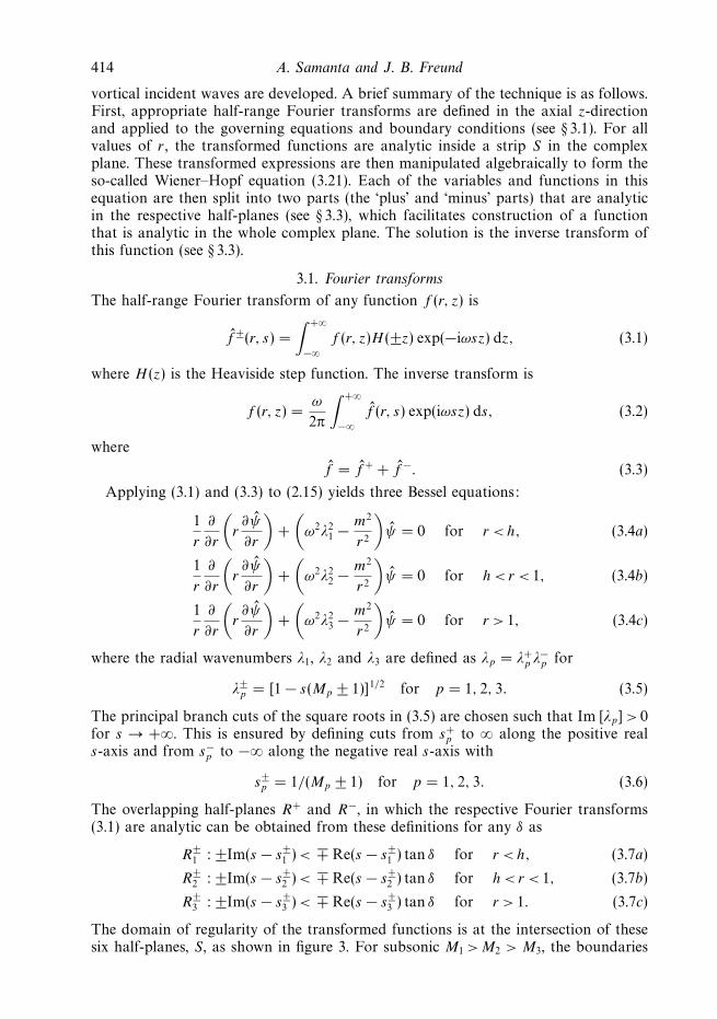
The domain of regularity of the transformed functions is at the intersection of thesesix half-planes, S, as shown in figure 3. For subsonic M1 > M2 > M3, the boundaries


–10 –5 0 5

Γ

10–10

–5

0

5

δ

δ

10

Instability

Acoustic

Branch Branch

zeros/pole

zeros/poles

cutcut

R3–

S

Im(s

)

Re(s)

R1+

Figure 3. The zeros (◦) and poles (×) of the kernel given by (3.22) are shown for δ = π/4.The parameters are M1 = 0.55, M2 = 0.3, M3 = 0.1, h = 0.9, ω = 5, and m = 1. Also note thedefinitions of the R+

1 and R−3 half-planes, the inverse Fourier transform contour Γ and the

shaded strip S.

of S are set by R+1 and R−

3 . An acceptable inverse Fourier transform path lies in S

along Γ defined by arg s = δ.A general solution of (3.4) for p = 1, 2, 3 is

ψ̂(r, s) = Ap(s)Jm(λpωr) + Bp(s)H(1)m (λpωr), (3.8)

where Jm and H(1)m are respectively the order-m Bessel and Hankel functions of the

first kind. Setting B1 = 0 ensures regular behaviour of ψ̂ as r → 0. Similarly, settingA3 = 0 ensures radiation at infinity given that Im [λ3ω] in S is positive, for thedefinitions of the radial wavenumbers and their branch cuts used in the analysis.Thus, the solution of (3.4) is

ψ̂(r, s) =

⎧⎪⎨⎪⎩

A1(s)Jm(λ1ωr) for r <h,

A2(s)Jm(λ2ωr) + B2(s)H(1)m (λ2ωr) for h < r < 1,

B3(s)H(1)m (λ3ωr) for r > 1.

(3.9)

The undetermined constants in (3.9) are found by Fourier transforming theboundary conditions. The transformed vortex sheet displacements, ξ̂+(s) and γ̂ (s),corresponding to the outer and inner shear layers, are defined according to (3.1). Theouter sheet exists only for z > 0, and thus only has the ‘plus’ transformed part of ξ̂ .In addition, for convenience, two other quantities are defined that correspond to thepressure jump across the vortex sheets. These jumps are in the scattered pressures; thetotal pressure is, of course, continuous across the sheets. By the definition of scatteredpressure in (2.18) and (2.20) these jumps are

p̂o(s) =

∫ +∞

−∞

[(−iω+M3

∂

∂z

)ψ(1+, z)−

(−iω+M2

∂

∂z

)ψ(1−, z)

]exp(−iωsz)dz (3.10)


for the outer shear layer (z > 0) and the shroud walls (z < 0) and

p̂i(s) =

∫ +∞

−∞

[(−iω+M2

∂

∂z

)ψ(h+, z)−

(−iω+M1

∂

∂z

)ψ(h−, z)

]exp(−iωsz)dz (3.11)

for the inner shear layer (−∞ <z < ∞). Applying (3.9) to (3.10) and (3.11) yields

p̂o(s) = −iω{

(1 − sM3) B3(s) H(1)m (λ3ω)

− (1 − sM2) [A2(s) Jm(λ2ω) + B2(s) H(1)m (λ2ω)]

}, (3.12)

and

p̂i(s) = −iω{

(1 − sM2) [A2(s) Jm(λ2ωh) + B2(s) H(1)m (λ2ωh)]

− (1 − sM1) A1(s) Jm(λ1ωh)}. (3.13)

Taking a similar approach, applying (3.9) to (2.17) and using (2.16), the Fouriertransform of the kinematic boundary condition on the outer vortex sheet (2.17)becomes

−i(1 − sM2)ξ̂+(s) = λ2{A2(s)J′

m(λ2ω) + B2(s)H(1)′m (λ2ω)}, (3.14a)

−i(1 − sM3)ξ̂+(s) = λ3B3(s)H(1)′

m (λ3ω). (3.14b)

Here primes denote derivative with respect to the argument of the function. The innershear layer displacement given by (2.19) can similarly be transformed to

−i(1 − sM1)γ̂ (s) = λ1{A1(s)J′m(λ1ωh)}, (3.15a)

−i(1 − sM2)γ̂ (s) = λ2{A2(s)J′m(λ2ωh) + B2(s)H(1)′

m (λ2ωh)}. (3.15b)

The Fourier transform of the dynamic boundary condition on the outer vortex sheet(2.18) with application of (3.10) and (2.14) leads to

p̂+o (s) = B+

mnΨmn(1)1 − μ+

mnM2

μ+mn − s

. (3.16)

The corresponding transform of (2.20) using (3.11) reduces to

p̂i(s) = 0, (3.17)

as it must since for the inner shear layer both the total pressures and the scatteredpressures are continuous for our choices of incident waves.

To determine the constants in (3.9), we sequentially combine (3.13), (3.17), (3.15),and (3.14) to arrive at

A1(s) = − i

λ2

(1 − sM2)2

1 − sM1

ξ̂+(s)

Jm(λ1ωh)

H(1)m (λ2ωh) + R(s)Jm(λ2ωh)

H(1)′m (λ2ω) + R(s)J′

m(λ2ω), (3.18a)

A2(s) = − i

λ2

(1 − sM2)ξ̂+(s)R(s)

H(1)′m (λ2ω) + R(s)J′

m(λ2ω), (3.18b)

B2(s) = − i

λ2

(1 − sM2)ξ̂+(s)

H(1)′m (λ2ω) + R(s)J′

m(λ2ω), (3.18c)

B3(s) = − i

λ3

(1 − sM3)ξ̂+(s)

H(1)′m (λ3ω)

, (3.18d)


where we have defined

R(s) =λ(s)Jm(λ1ωh)H(1)′

m (λ2ωh) − H(1)m (λ2ωh)J′

m(λ1ωh)

Jm(λ2ωh)J′m(λ1ωh) − λ(s)Jm(λ1ωh)J′

m(λ2ωh), (3.19)

with

λ(s) =λ2

λ1

(1 − sM1)2

(1 − sM2)2. (3.20)

The one remaining unknown in (3.18) is ξ̂+, the Fourier transform of the outer vortexsheet displacement. To determine ξ̂+ we substitute (3.18b)–(3.18d ) into (3.12) andutilize p̂o = p̂+

o + p̂−o to arrive at

K(s)ξ̂+(s) − p̂+o (s) = p̂−

o (s), (3.21)

where p̂+o is given by (3.16). This manipulation introduces p̂−

o , the pressure jumpacross the shroud wall, as a second unknown. Equation (3.21) is the Wiener–Hopfequation with kernel

K(s) = ω

{(1 − sM2)

2

λ2

[H(1)

m (λ2ω) + R(s)Jm(λ2ω)

H(1)′m (λ2ω) + R(s)J′

m(λ2ω)

]− (1 − sM3)

2

λ3

H(1)m (λ3ω)

H(1)′m (λ3ω)

}. (3.22)

Though not obvious as formulated, the kernel so-obtained is equivalent to the oneobtained by Taylor et al. (1993) in their ‘plane B sub-problem’, which they solvefor acoustic interactions in the low-frequency limit. We use it to obtain scatteringsolutions for finite-wavelength acoustic and vorticity incident waves.

3.2. The kernel

The poles and zeros of the kernel define the characteristics of the problem, the exactlocations of which depend upon the parameters chosen. Since the analysis and thesubsequent contour integrations depend upon the locations of these zeros/poles, itis important to identify their characteristics (e.g. acoustic or instability modes) andlocations. Figure 3 shows the poles and zeros of (3.22) for one set of parameters. Thereare two basic types of zeros and poles. The first correspond to the acoustic shroudmodes and these zeros and poles lie along a curve that asymptotically approachesπ/2 − δ for large |s|. The acoustic poles come from the denominators of (3.22),and most of them come from the first term. Since this first term’s denominatorcorresponds to the characteristic equation of the infinite shroud (see (4.3)), poles fromthis denominator match the acoustic modes of an infinite shroud. From figure 4(b),it is clear that the second-term denominator contributes only two poles for allparameters investigated. This second term of (3.22) can be thought of as a correctionterm that accounts for finite termination of the infinite shroud, as evidenced by M3

appearing only in this term. The poles lying on the real axis for δ → 0 (figure 4a)correspond to propagating waves, whereas the disturbances associated with the restdecay away from the shroud exit. In § 4 and § 6, where we select specific incidentand reflected waves, we focus on these propagating waves. Nevertheless, for a shortdistance between the shroud exit and the nozzle lip upstream of it, some of thedecaying acoustic components of the reflected wave may be important.

The second type of poles and zeros corresponds to the Helmholtz instability modesof the vortex sheets. These zeros and pole sit in the fourth quadrant of the complexplane, as seen in figure 3. The two zeros correspond to modes of the shear layersdownstream of the shroud exit, and the pole corresponds to that of the inner shearlayer upstream of the exit. Unlike the low-frequency case considered by Taylor et al.


–5 0 5 10–10

–10

–5

0

5

Γ

Γ

10

Im(s

)

Re(s) Re(s)

(a) (b)

–2 0 2

–2

0

2

Figure 4. (a) Example locations of the zeros (◦) and poles (×) of K(s) in (3.22) for δ → 0.(b) Enlarged view of (a) which in addition identifies �, the poles arising from the second termin (3.22) (see text). Parameters are same as in figure 3.

(1993), for disturbances considered here with wavelengths comparable to the shrouddiameter or shorter, the zero and the pole for the inner shear layer are close to eachother. This is because of the exponential decay of the disturbances away from thevortex sheet. For moderate wavelengths they only interact weakly with the shroudwalls and the instabilities are nearly the same regardless of their confinement. Thoughweak, this interaction is still important from the perspective of generating sound.

We use a Newton–Raphson iterative scheme to compute these zeros and poles withthe derivatives computed using a scheme by Ridders (1982). The close lying zero–polepairs require good initial estimates.

3.3. General solutions

A multiplicative split of the kernel (3.22) can be carried out as K(s) = K+(s)K−(s),where the two factors K+ and K− are analytic, non-zero and have at most algebraicgrowth in their respective half-planes. However, it is more convenient to factor theinstability zeros sz1

and sz2and the pole sp out of the kernel before splitting it

(e.g. Gabard & Astley 2006). This facilitates the application of the residue theoremin determining the instability part of the scattered solutions (see (3.36), (3.37)).Accordingly, for incident acoustic waves we take

K(s) = K̃+(s)K̃−(s)U (s), (3.23)

where

U (s) =(s − sz1

)(s − sz2

)/(s − sp). (3.24)

For an incident vorticity wave, the inner vortex sheet pole acts as the incident mode,so streamwise wavenumber μ+

mn from (2.14) is μ+mn = sp . Using (3.24) in this case to

compute terms such as K̃−(μ+mn) from (A 1) in the Appendix and (3.23), as needed

later in (3.30), is numerically problematic, as U (μ+mn) becomes singular. It is then best

not to factor out sp as in (3.24). Given the close proximity of sz1and sp it is also

best to leave sz1unfactored. The kernel integration contour C (see Appendix A.1) is

simply deformed around both. Thus for the incident vorticity case

U (s) =(s − sz2

). (3.25)


In both cases, K̃+ and K̃− are split functions of K/U . Substituting (3.23) into (3.21)yields

U (s)K̃+(s)ξ̂+(s) − p̂+o (s)

K̃−(s)=

p̂−o (s)

K̃−(s). (3.26)

The first term on the left-hand side is analytic in R+, whereas the right-hand-sideterm is analytic in R−. Unfortunately, p̂+

o has a pole at s = μ+mn (see (3.16)) so that

the second term is not analytic in R−. This is resolved by the rearrangement

U (s)K̃+(s)ξ̂+(s) − p̂+o (s)

K̃−(μ+mn)

=p̂−

o (s)

K̃−(s)+ p̂+

o (s)

[1

K̃−(s)− 1

K̃−(μ+mn)

]. (3.27)

Since K̃− is analytic in R−, K̃−(μ+mn) is just a finite constant, so the entire left-hand

side is regular in R+. Also, the singularity that p̂+o had in R− is cancelled by the

corresponding zero of the bracketed term on the right. This second term on the right-hand side is thus appropriately analytic in R−. As formulated, (3.27) is regular in S,so by the usual analyticity arguments each side is equal to some common functionthat is analytic in the entire complex s-plane.

By the extended Liouville’s theorem (e.g. Noble 1988), which requires such functionsto be polynomials, we have

U (s)K̃+(s)ξ̂+(s) − p̂+o (s)

K̃−(μ+mn)

=p̂−

o (s)

K̃−(s)+ p̂+

o (s)

[1

K̃−(s)− 1

K̃−(μ+mn)

]

=

N∑k=0

aksk as |s| → ∞. (3.28)

The next step is to use the asymptotic forms of the above expressions to determinethe ak in the sum. All the terms in (3.28) must have the same behaviour for large |s|,so we consider only the first term, which is the easiest to analyse. Asymptotic forms ofcertain sub-components of (3.22) are provided in the Appendix, § A.2. To find K̃+(s)for large |s|, we start by considering K(s). In the strip S, λ3ω has a positive imaginarypart (see the argument made before (3.9)), so for |s| → ∞ the Hankel function ratioinvolving M3 in (3.22) is negative (using (A 3)), and thus K(s) can be approximatedas K(s) ≈ (1 − sM2)

2/λ2 + (1 − sM3)2/λ3. This gives K(s) ∼ s for large |s| in S. From

(3.24) and (3.25) we have U (s) ∼ s as |s| → ∞. Thus K(s)/U (s) ∼ 1 as |s| → ∞, whichgives K̃+(s) = K̃−(s) ∼ 1, with the phase remaining the same, as |s| → ∞. To find the

large-|s| behaviour of ξ̂+(s), we use the Kutta condition (2.21) and the definition of

the Fourier transform (3.1), which gives ψ̂(1, s) ∼ s−5/2. Using this in (3.9) for r > 1indicates that B3(s) ∼ s−5/2, since Im [λ3ω] > 0. Also, since λ3(s) ∼ s as |s| → ∞ by

(3.5), from (3.14b) we conclude that ξ̂+(s) ∼ s−5/2 as |s| → ∞. Thus

U (s)K̃+(s)ξ̂+(s) ∼ s1+0−5/2 ∼ s−3/2 as |s| → ∞. (3.29)

This requires ak = 0, for all k, in (3.28), which upon application of (3.16) yields

ξ̂+(s) = B+mnΨmn(1)

1 − μ+mnM2

(μ+mn − s)K̃−(μ+

mn)K̃+(s)U (s). (3.30)

The same procedure may be repeated using (2.8) to obtain the no-vortex-sheddingsolution. Introducing the complex vortex shedding parameter γ used by Gabard &


–5 0 5 10–10

–10

–5

0

5

10

R+ R+R– R–

R+

R+R–

R–

Im(s

)

(a)

(c) (d )

(b)

–5 0 5 10–10

–10

–5

0

5

10

–5 0 5 10–10

–10

–5

0

ΓΓ

ΓΓ

5

10

Im(s

)

Re(s) Re(s)–5 0 5 10

–10–10

–5

0

5

10

Figure 5. The zeros (◦) and the poles (×) of (3.22) in the complex plane as δ changes fromδ → π/2 to δ → 0. The parameters are the same as in figure 3 with (a) δ = π/2, (b) π/3,(c) π/6 and (d ) π/18. Note how the instability zeros and pole lying in the fourth quadranttend to move from R− to R+ between (c) and (d ) which requires deformation of Γ . Also,the complex conjugates of the instability zeros/pole can be seen in (a), which correspond todecaying convective instability modes and are not included in the analysis.

Astley (2006) and Rienstra (1984) generalizes (3.30) to

ξ̂+(s) = B+mnΨmn(1)

1 − μ+mnM2

(μ+mn − sz2

)K̃−(μ+mn)K̃+(s)U (s)

(s − sz2

μ+mn − s

+ γ

), (3.31)

where 0 < |γ | < 1. The special cases are γ = 1, which reduces to (3.30) and is the fullKutta condition, and γ = 0, the no-vortex-shedding condition.

The physical solutions we seek are for real-valued ω, which corresponds to δ → 0.This rotates the inverse transform contour Γ in figure 5(a), to be parallel to the realaxis (see figure 4a). As a result Γ now extends from −∞ + 0i to ∞ − 0i, crossing thereal s-axis at some intermediate point so that analytic continuity is preserved. Figure 5depicts how the various poles and zeros of the kernel move as δ → 0. The instabilityzeros/pole do not move with this rotation and so Γ must be deformed aroundthem to ensure they remain in R− and analytic continuity is preserved (figure 5d ). Inpractice, however, a simple application of the residue theorem is sufficient to explicitlyidentify the contribution of these instability modes. We must also be aware of themovement of the acoustic poles and zeros and account for their crossing, if any, asΓ is rotated. In a related problem, Munt (1977) carried out an extensive asymptoticand numerical analysis to locate the kernel zeros and poles for a wide range of flowparameters and different δ to conclude that the acoustic zeros/poles do not cross Γ


as δ → 0. Such an analysis is intractable in cases like the present (e.g. Taylor et al.1993). However, we have made careful observations of the movement of acousticzeros/poles as δ varies from π/2, where causality is satisfied, to δ = 0, to choose Γ .Experiments where a pole/zero was purposely placed on the wrong side of Γ yieldeda final solution that clearly violated causality, which also supports our choice of Γ infigure 4(b).

The solution of the scattered acoustic potential field is then found by firstsubstituting (3.30) and (3.18) into (3.9) and then using (3.2) to arrive at

ψa(r, z) =

⎧⎪⎪⎪⎪⎪⎪⎪⎨⎪⎪⎪⎪⎪⎪⎪⎩

ω

2πi

∫Γ

(1 − sM2)2

(1 − sM1)

T1(r, s)ξ̂+(s)

λ2

exp(iωsz) ds for r < h,

ω

2πi

∫Γ

(1 − sM2)T2(r, s)ξ̂+(s)

λ2

exp(iωsz) ds for h< r < 1,

ω

2πi

∫Γ

(1 − sM3)T3(r, s)ξ̂+(s)

λ3

exp(iωsz) ds for r > 1,

(3.32)

where

T1(r, s) =Jm(λ1ωr)

Jm(λ1ωh)

H(1)m (λ2ωh) + R(s)Jm(λ2ωh)

H(1)′m (λ2ω) + R(s)J′

m(λ2ω), (3.33a)

T2(r, s) =H(1)

m (λ2ωr) + R(s)Jm(λ2ωr)

H(1)′m (λ2ω) + R(s)J′

m(λ2ω), (3.33b)

T3(r, s) =H(1)

m (λ3ωr)

H(1)′m (λ3ω)

. (3.33c)

The solution for the scattered pressure is easily found from (3.32) via the linearizedunsteady Bernoulli equation,

p = −(

∂ψ

∂t+ M

∂ψ

∂z

). (3.34)

Hence, the scattered acoustic pressure field has the following general solution:

pa(r, z) =

⎧⎪⎪⎪⎪⎪⎪⎨⎪⎪⎪⎪⎪⎪⎩

ω2

2π

∫Γ

(1 − sM2)2

λ2

T1(r, s) ξ̂+(s) exp(iωsz) ds for r < h,

ω2

2π

∫Γ

(1 − sM2)2

λ2

T2(r, s) ξ̂+(s) exp(iωsz) ds for h < r < 1,

ω2

2π

∫Γ

(1 − sM3)2

λ3

T3(r, s) ξ̂+(s) exp(iωsz) ds for r > 1.

(3.35)

As mentioned above, the instability part of the scattered field is obtained byapplying residue theorem for sz1

and sz2, which appear as simple poles in (3.32)

and (3.35) via the U (s) factor in (3.30). For incident vorticity waves, however,since sz1

was not included in (3.25), the scattered field due to the inner vorticitywave is included in (3.32). The expression for the scattered instability potential is


Cylindrical wall

r

zM1

M2

h

1

Jet

Co-flowIncident wave

Vortex sheet

Figure 6. Schematic of the infinite shroud with co-flow used to obtainthe acoustic incident waves.

then

ψs(r, z) = ω∑

s ′

exp(iωs ′z) lims→s ′

[ξ̂+(s)]

× H (z)

⎧⎪⎪⎪⎨⎪⎪⎪⎩

(1 − s ′M2)2

(1 − s ′M1)lims→s ′[T1(r, s)/λ2] for r < h,

(1 − s ′M2) lims→s ′[T2(r, s)/λ2] for h < r < 1,

(1 − s ′M3) lims→s ′[T3(r, s)/λ3] for r > 1.

(3.36)

Similarly, the scattered instability pressure is

ps(r, z) = iω2∑

s ′

exp(iωs ′z) lims→s ′

[ξ̂+(s)]

× H (z)

⎧⎪⎨⎪⎩

(1 − s ′M2)2 lims→s ′[T1(r, s)/λ2] for r <h,

(1 − s ′M2)2 lims→s ′[T2(r, s)/λ2] for h < r < 1,

(1 − s ′M3)2 lims→s ′[T3(r, s)/λ3] for r > 1,

(3.37)

where

lims→s′si �=s′

[ξ̂+(s)] = B+mnΨmn(1)

(1 − μ+mnM2)(s

′ − sp)

(μ+mn − s ′)K̃−(μ+

mn)K̃+(s ′)(s ′ − si), (3.38)

where s ′ and si are respectively sz1or sz2

or vice versa depending upon which instabilitywave pressure field is sought. The total scattered potential and pressure are then

ψ(r, z) = ψa(r, z) + ψs(r, z) and p(r, z) = pa(r, z) + ps(r, z), (3.39)

with the total field obtained by simply adding the incident field. Though not obviousby visual inspection, it can be confirmed that these solutions degenerate to those ofMunt (1977) and Taylor et al. (1993) in the appropriate limits (Samanta 2008).

4. Incident wavesWe first analyse the acoustic-type incident wave in the following subsection, which

has previously been studied only for m = 0 in the long-wavelength limit for thisconfiguration. We then take up the instability-type case in § 4.2.

4.1. Acoustic-type incident waves

In this case the incident waves are the right-propagating modes in an infinite shroudwith two concentric streams as shown in figure 6. The starting points are theright-moving + components of (2.10), which were expressed in terms of the unknown


mode shape functions Ψmn. The governing differential equations (2.15a, b) are satisfiedby

Ψmn(r) =

⎧⎪⎪⎨⎪⎪⎩

Jm(rαmn), r <h,(1 − μ+

mnM1

1 − μ+mnM2

)Jm(hαmn)

[Jm(rβmn)H(1)′

m (βmn) − H(1)m (rβmn)J′

m(βmn)

Jm(hβmn)H(1)′m (βmn) − H(1)

m (hβmn)J′m(βmn)

], r >h,

(4.1)where for axial wavenumber μ+

mn the radial wavenumbers

αmn = ω

√(1 − μ+

mnM1)2 − μ+mn

2 and βmn = ω

√(1 − μ+

mnM2)2 − μ+mn

2 (4.2)

satisfy the hard wall (2.16) and the dynamic (2.20) boundary conditions. The dispersionrelationship, which is obtained via (2.19), provides the final constraint on α, β and μ:

Λ(z) ≡ z2(1 − zM1)2Jm(hz1)[J

′m(hz2)H

(1)′m (z2) − H(1)′

m (hz2)J′m(z2)]

− z1(1 − zM2)2J′

m(hz1)[Jm(hz2)H(1)′m (z2) − H(1)

m (hz2)J′m(z2)] = 0, (4.3)

with

z1 = ω√

(1 − zM1)2 − z2 and z2 = ω√

(1 − zM2)2 − z2. (4.4)

For any m, the nth real-valued μ+mn roots of (4.3) represents the propagating mode

(m, n). The requirement that the radial wavenumbers α and β in (4.2) be real valuedand positive quantities restricts μ+

mn as

− 1

1 − M2

<μ+mn <

1

1 + M1

. (4.5)

Finally, to be incident on the shroud exit the waves must have non-negative groupvelocity,

dω

dμ+mn

> 0. (4.6)

The amplitude B+mn in (2.14) is taken to be unity for incident acoustic waves.

4.2. Instability-type incident waves

Kelvin–Helmholtz instability incident waves satisfy the same equations and boundaryconditions as the acoustic modes presented in the last section, but specialconsiderations are warranted to cope with their exponential growth. To constructa finite-amplitude incident wave we must consider a finite-length inner vortex sheet.

We assume that the origin of the instability wave is an inner nozzle lip at adistance zo upstream of the shroud exit. This upstream distance is assumed to besufficiently large to decouple the nozzle from the shroud exit. The wavenumber ofthis instability wave matches sp defined in (3.24), which is the pole of the kernel (3.22)corresponding to the inner-sheet instability mode. This pole is a zero of the kernelfor the configuration shown in figure 7. For incident quasi-plane waves as in Tayloret al. (1993), the incident instability wave can be simply obtained from (2.14) sinceΨ01(r) = 1. The more general incident waves sought here require explicit solutions forΨmn(r), which can also be solved using a Wiener–Hopf formulation.

Since a similar problem setup (figure 7) is described in detail by Taylor et al. (1993),and extension to finite wavelengths is as discussed in § 3 of the present paper forthe finite-shroud problem, only a cursory overview is provided here. The governing


Cylindrical wall

Nozzler

z

M2

M1

h

1

Jet

Co-flowIncident wave

Vortex sheet

Figure 7. Schematic of the infinite shroud with an inner nozzle and co-flow used to obtainthe instability incident waves.

equations are the same as (2.1a, b). The wall boundary condition (2.2) is applied to theinner and outer surfaces of the nozzle and the outer, now-infinite, shroud. The usualvortex sheet boundary conditions (2.3) and (2.4), the nozzle-lip Kutta condition (2.7),and the causality requirement complete the problem description. The solution thenfollows the procedure described in § 2.1 and § 3, yielding scattered acoustic potential

ψa(r, z) =

⎧⎪⎪⎨⎪⎪⎩

ω

2πi

∫Γ

(1 − sM1)Y1(r, s)β̂+(s)

λ1

exp(iωsz) ds for r <h,

ω

2πi

∫Γ

(1 − sM2)Y2(r, s)β̂+(s)

λ2

exp(iωsz) ds for h< r < 1.

(4.7)

This is nearly the same as (3.32), but β̂+(s) is the Fourier-transformed vortex sheetdisplacement for this auxiliary problem and

Y1(r, s) =Jm(λ1ωr)

J′m(λ1ωh)

, (4.8a)

Y2(r, s) =Jm(λ2ωr)H(1)′

m (λ2ω) − H(1)m (λ2ωr)J′

m(λ2ω)

J′m(λ2ωh)H(1)′

m (λ2ω) − H(1)′m (λ2ωh)J′

m(λ2ω). (4.8b)

The transformed vortex sheet displacement is given by

β̂+(s) = Ψmn(h)(1 − μ+

mnM1)

(μ+mn − s)K̃−

1 (μ+mn)K̃+

1 (s)(s − so). (4.9)

Here μ+mn is the wavenumber of the acoustic wave incident from inside the nozzle that

is used to seed the instability wave in this auxiliary problem. In (4.9), so is the zerocorresponding to the shear layer instability, which matches the pole sp for the finiteshroud in (3.24), and Ψmn(r) = Jm(αmnr) with αmn being a solution of Λ(z) = J′

m(z) = 0.This incident acoustic mode, which only propagates for ω > (1 − M2

1 )1/2αmn sets alower bound of ω = (1 − M2

1 )1/2αm1 for the vorticity frequency. The kernel K1(s) in(4.9) is

K1(s) = ω

{(1 − sM1)

2

λ1

Jm(λ1ωh)

J′m(λ1ωh)

− (1 − sM2)2

λ2

Jm(λ2ωh)H(1)′m (λ2ω) − H(1)

m (λ2ωh)J′m(λ2ω)

J′m(λ2ωh)H(1)′

m (λ2ω) − H(1)′m (λ2ωh)J′

m(λ2ω)

}. (4.10)


It is clear from (4.9) that so appears as a simple pole in (4.7), so the scattered instabilitypotential is easily obtained simply via its residue,

ψs(r, z) = ω exp(iωsoz) lims→so

[β̂+(s)]

× H (z)

{(1 − soM1) lims→so

[Y1(r, s)/λ1] for r <h,

(1 − soM2) lims→so[Y2(r, s)/λ2] for h< r < 1,

(4.11)

to yield the incident instability wave for the full problem. Comparing (4.11) with(2.14), it is easy to see that

B+mn = ω exp(−iωspzo) lim

s→sp

[β̂+(s)], (4.12)

and the mode shape is

Ψmn(r) = H (z − zo)

{(1 − spM1) lims→sp

[Y1(r, s)/λ1] for r <h,

(1 − spM2) lims→sp[Y2(r, s)/λ2] for h< r < 1,

(4.13)

with μ+mn = so = sp . The factor exp(−iωspzo) appears in (4.12) since the vortex sheet

originates at zo. Unlike in § 3.3 we are not concerned with the scattered acoustic fieldhere and thus the full solution of this auxiliary problem is unnecessary.

5. Near-field solutionsThe numerical methods to accurately evaluate (3.35) are summarized in the

Appendix. In this section, we present the near-field solutions for pressure for incidentacoustic and vorticity waves. These solutions support exponentially growing instabilitywaves, which are of course not physically realizable. However, the utility of themodel depends primarily upon how well the shape and dispersion characteristicsof the instability waves represent the pressure fields associated with the turbulencestructures at the shroud exit. This near-field pressure similarity has recently beenconfirmed by matching the predicted near fields of instability waves with the near-field pressure of turbulence structures in a high-Reynolds-number jet (Suzuki &Colonius 2006). In addition, studies on large coherent structures in turbulent shearflows (e.g. Strange & Crighton 1983; Gaster, Kit & Wygnanski 1985) have shownthat linear theory can accurately predict the local transverse mode shapes and phasecharacteristics of instabilities along with their dispersion relations, even for strongnonlinear disturbances. These aspects have also been discussed in detail by Crighton(1992) in the context of linear models such as the present. Amplitude predictionswould, of course, require additional procedures which are beyond the scope of thecurrent theoretical study and would probably involve large-scale simulations.

5.1. Incident acoustic wave

For an example solution, we choose h = 0.65, M1 = 0.9, M2 = 0.25, M3 = 0.1, andω = 4.5 with the azimuthal mode number m = 1. For these input parameters thereis only one right-propagating acoustic mode (n = 1). Figure 8(a) shows the incidentacoustic wave and figure 8(b) shows the entire near-field acoustic component ofpressure. The reflected waves moving leftward inside the shroud and part of thescattered wave field are shown in figure 8(c). Figures 8(d ) and 8(e) show the instabilitywaves excited on the inner and outer vortex sheets, respectively. The outer vortexsheet is perturbed with shorter wavelengths, as expected for the selected flow Mach


(a) (b)

(c)

4

1.0

0.5

–1.5 –1.0 –0.5 0

3

r

r

2

1

–1 0 1 2 3

(e)

4

3

r

z z

2

1

–1 0 1 2 3

( f )

4

3

2

1

–1 0 1 2 3

4

3

2

1

–1 0 1 2 3

(d )

4

3

2

1

–1 0 1 2 3

Figure 8. Real part of the pressure for the incident acoustic mode (1, 1): (a) the incidentwave; (b) the acoustic part of the pressure field; (c) the scattered and reflected acoustic pressurewaves; (d ) the instability wave of the inner shear layer; (e) the instability wave of the outershear layer; and (f ) the total pressure field. Grey levels indicate pressure between ±0.4 for anincident wave with unit amplitude.

numbers. The vorticity wave on the outer sheet is also of higher amplitude, which canbe seen in figure 8(f ), which shows the complete solution. The outer wave is expectedto be of much higher amplitude since it is seeded at a sharp edge, and thus should bemore receptive than the inner. For example, at z = 2, the outer wave has an amplitude


almost 108 higher than the inner. The instability waves grow exponentially in z butdecay exponentially in the r-direction yielding the wedge shapes for the influence ofthe vorticity waves.

5.2. Incident vorticity wave

For this demonstration, we retain the same flow parameters as in the previoussection for the acoustic wave. Figure 9(a) shows the incident vorticity wave thatoriginates from the assumed inner nozzle lip at zo = −1.5. Figure 9(b) shows thescattered acoustic field generated by the incident instability wave together with the(r > 1, z > 0) portion of this instability wave which, unlike in the preceding subsection,is computed in conjunction with the scattered acoustic field (see the Appendix, § A.1).Most of the energy of the incident vorticity wave transmits, but a portion is scatteredinto acoustic waves that seem to radiate outwards from the shroud edge and reflectback inside of the shroud (figure 9c). Figure 9(d ) shows the pressure associated withthe outer vortex sheet instability and figure 9(e) shows the total pressure field, asuperposition of the components shown in figures 9(b) and 9(d ). The vorticity wavesin z > 0 are of more comparable magnitude in this case. At z = 2 the outer waveamplitude is about 104 higher than the inner.

Figure 10 shows the field generated when there is no propagating reflected mode.The parameters are selected with reference to figure 14(a) so that the data point liesin the ‘no reflection’ zone. The non-propagating reflected waves are seen to decayover a very short upstream distance in figure 10(c). Figure 10(f ) shows the plot ofthe kernel poles and zeros for this case. As expected, there is no pole lying on thereal axis in between the left branch cut and the (Γ ) contour crossover point, whichis where the propagating reflected modes are found. In any such situation a pole isalways present between the branch points s−

1 and s−2 , as can be seen in figure 10(f ),

but it lies on the left branch cut. With changing parameters, this pole can move alongthe real axis. As it leaves the left branch cut it becomes a valid propagating reflectingmode for the system. However, for a given set of parameters, there might be multiplesuch poles with some of them as propagating modes and the rest lying on the cut(e.g. figure 4b).

6. Shroud-exit reflectivityIn this section we consider the acoustic wave reflected by the shroud exit, which

potentially closes a resonance loop as discussed in § 1.1.

6.1. Reflectivity formulation

Reflection coefficients for both acoustic and vortical incident waves can be definedusing the same framework. For each pair of incident and reflected modes we firstconsider the modal decomposition of the pressure field inside the shroud:

p(r, z) =

∞∑m=−∞

∞∑n=1

[A+mnexp(iμ+

mnωz) + A−mnexp(iμ−

mnωz)]Ψmn(r), (6.1)

which is analogous to (2.10) for the velocity potential. Here A±mn are the right- (+)

and left- (−) propagating pressure wave amplitudes. The reflection coefficient for the(m, l) mode reflection of an incident (m, n) mode is defined as

Rmnl =A−

ml

A+mn

. (6.2)


(a) (b)

(c)

4

1.0

0.5

–1.5 –1.0 –0.5 0

3

r

r

2

1

–1 0 1 2 3

(e)

4

3

r

z

zz

2

1

–1 0 1 2 3

4

3

2

1

–1 0 1 2 3

(d )

4

3

2

1

–1 0 1 2 3

Figure 9. Real part of the pressure for the incident instability mode for h = 0.65,M1 = 0.09,M2 = 0.25, M3 = 0.1, ω = 4.5,m = 1: (a) the incident wave; (b) the acoustic part of the pressurefield and inner instability wave superimposed; (c) the scattered and reflected acoustic pressurewaves; (d ) the instability wave of the outer shear layer; and (e) the total pressure field. Greylevels indicate pressure between ±0.4. The seed acoustic wave (see § 4.2) has unity amplitude.

The incident wave amplitude A+mn is straightforward to identify. By applying (3.34)

to (2.14), we can write the pressure field inside the shroud as

pi(r, z) =

{iω(1 − μ+

mnM1)B+mnΨmn(r) exp(iωμ+

mnz) for r <h,

iω(1 − μ+mnM2)B

+mnΨmn(r) exp(iωμ+

mnz) for h< r < 1.(6.3)


(a) (b)

(c)

4

1.0

0.5

–1.5 –1.0 –0.5 0

3

r

r

2

1

–1 0 1 2 3

(e)

4

3

r

z

z z

zz

2

1

–1 –20 1 2 3

( f )

–2

0

0

Im(s

)

Re(s)2

2

Γ

4

3

2

1

–1 0 1 2 3

(d )

4

3

2

1

–1 0 1 2 3

Figure 10. (a–e) Same as figure 9 for M1 = 0.7, M2 = 0.25, M3 = 0.1, h = 0.8, ω = 3.5, andm = 1. (f ) Location of the zeros (◦) and poles (×) of K(s) in (3.22) as δ → 0.

Comparing (6.3) to (6.1) we see that the amplitude of the incident wave is thus

A+mn =

{iωB+

mn(1 − μ+mnM1) for r <h,

iωB+mn(1 − μ+

mnM2) for h< r < 1.(6.4)

For incident acoustic waves we take B+mn = 1, while for incident vorticity waves it

is given by (4.12). Consequently, for incident instability waves A+mn is the pressure

amplitude at the shroud exit.


Computing the pressure amplitude A−ml of the reflected mode is more involved. The

net scattered pressure is the sum of the acoustic and instability parts as given by(3.35) and (3.37), respectively. The contour integral in (3.35) can be evaluated forindividual wave components of the full solution using the residue theorem. Since weseek amplitudes of the modes inside the shroud (r < 1, z < 0), only the poles lyingbelow Γ in the lower-half-plane (R+) are needed. This is because the transformedfields, as defined, are analytic in R− for z < 0. So, the poles corresponding to thewaves inside the shroud (z < 0) must only lie in R+. In order to be non-decaying theymust also lie on the real axis between the left and right branch cuts (see figure 3b).Reflectivities are only well-defined for these propagating reflected modes (m, l), soto compute them the field inside the shroud can be written via the residue theoremas

p(r, z) = −iω2

∞∑l=1

∞∑m=−∞

exp(iωμ−mlz) (1 − μ−

mlM2)2

× lims→μ−

ml

[ξ̂+(s)]

{lims→μ−

ml(T1(r, s)/λ2) for r < h,

lims→μ−ml

(T2(r, s)/λ2) for h < r < 1.(6.5)

The next task is to write both cases of (6.5) in a form similar to (6.1) to identifyA−

ml . The shapes of the reflected modes inside the shroud are the same as the incidentacoustic modes given by (4.1), but for a wavenumber of μ−

ml , and therefore arealready known. To evaluate the limits in (6.5) we start with (3.5), where we can solveλ2

p = (1 − sMp)2 − s2 for s as

s =−Mp ±

√1 −

(1 − M2

p

)λ2

p

1 − M2p

for p = 1, 2. (6.6)

Likewise, from (4.2) it can be shown that

μ−ml =

−M1 −√

1 −(1 − M2

1

)α2

ml

/ω2

1 − M21

=−M2 −

√1 −

(1 − M2

2

)β2

ml

/ω2

1 − M22

. (6.7)

Together, these indicate that as s → μ−ml

λ1 → αml/ω and λ2 → βml/ω. (6.8)

To explicitly evaluate the factors involving T1 in (6.5) for the r < h case we start withits definition (3.33a), substitute R(s) from (3.19) and employ (4.3). Then taking thelimit as s → μ−

ml yields

lims→μ−

ml

T1(r, s) = βml(1 − μ−mlM1)

2Ψml(r)J′m(βmlh)H(1)

m (βmlh) − H(1)′m (βmlh)Jm(βmlh)

Λ′(μ−ml)

, (6.9)

where we have also used (4.1) for r < h and (6.8). Substituting (6.9) in (6.5) yields

p(r, z) = −iω3

∞∑l=1

∞∑m=−∞

exp(iωμ−mlz)(1 − μ−

mlM1)2(1 − μ−

mlM2)2ξ̂+(μ−

ml)

× J′m(βmlh)H(1)

m (βmlh) − H(1)′m (βmlh)Jm(βmlh)

Λ′(μ−ml)

Ψml(r). (6.10)


Comparing this with (6.1) shows that

A−ml = −iω3 (1 − μ−

mlM1)2(1 − μ−

mlM2)2ξ̂+(μ−

ml)

Λ′(μ−ml)

× [J′m(βmlh)H(1)

m (βmlh) − H(1)′m (βmlh)Jm(βmlh)] for r < h. (6.11)

Similarly, for r > h we start by substituting (3.19) into (3.33b). Then we apply thelimit

lims→μ−

ml

[λ(s)

H(1)′m (λ2ωh)

H(1)′m (λ2ω)

Jm(λ1ωh) − H(1)m (λ2ωh)

H(1)′m (λ2ω)

J′m(λ1ωh)

]

= λ(s)J′m(λ2ωh)

J′m(λ2ω)

Jm(λ1ωh) − Jm(λ2ωh)

J′m(λ2ω)

J′m(λ1ωh), (6.12)

which is obtained from Λ(s) → 0 (see (4.3)) as s → μ−ml . Additional algebraic

manipulations lead to

lims→μ−

ml

T2(r, s) = αml

(1 − μ−mlM2)

3

(1 − μ−mlM1)

Ψml(r)

Λ′(μ−ml)

J′m(βml)H

(1)m (βmlh) − H(1)′

m (βml)Jm(βmlh)

Jm(αmlh)

× λ(μ−ml)H

(1)′m (βmlh)Jm(αmlh) − J′

m(αmlh)H(1)m (βmlh)

H(1)′m (βml)

. (6.13)

Substituting (6.13) in (6.5) yields the pressure for the r > h case,

p(r, z) = −iω3

∞∑l=1

∞∑m=−∞

exp(iωμ−mlz)

(1 − μ−mlM1)(1 − μ−

mlM2)3

Λ′(μ−ml)λ(μ−

ml)ξ̂+(μ−

ml)

× J′m(βml)H

(1)m (βmlh) − H(1)′

m (βml)Jm(βmlh)

Jm(αmlh)

× λ(μ−ml)H



H(1)′m (βml)

Ψml(r), (6.14)

which upon comparison with (6.1) gives

A−ml = −iω3 (1 − μ−

mlM1)(1 − μ−mlM2)

3

Λ′(μ−ml)λ(μ−

ml)ξ̂+(μ−

ml)J′m(βml)H

(1)m (βmlh) − H(1)′

m (βml)Jm(βmlh)

Jm(αmlh)

×λ(μ−ml)H



H(1)′m (βml)

for r > h. (6.15)


Finally, substituting (6.4), (6.11) and (6.15) into (6.2) yields the reflective coefficients:

Rmnl =

⎧⎪⎪⎪⎪⎪⎪⎪⎪⎪⎪⎪⎪⎪⎪⎪⎪⎪⎨⎪⎪⎪⎪⎪⎪⎪⎪⎪⎪⎪⎪⎪⎪⎪⎪⎪⎩

∣∣∣∣ω2 (1 − μ−mlM1)

2(1 − μ−mlM2)

2ξ̂+(μ−ml)

B+mn(1 − μ+

mnM1)Λ′(μ−ml)

× [J′m(βmlh)H(1)

m (βmlh) − H(1)′m (βmlh)Jm(βmlh)]

∣∣∣∣ for 0 < r < h,

∣∣∣∣ω2 (1 − μ−mlM1)(1 − μ−

mlM2)3ξ̂+(μ−

ml)

B+mn(1 − μ+

mnM2)Λ′(μ−ml)λ(μ−

ml)

×[λ(μ−

ml)H(1)′m (βmlh)Jm(αmlh) − J′


H(1)′m (βml)

]

×[

J′m(βml)H

(1)m (βmlh) − H(1)′

m (βml)Jm(βmlh)

Jm(αmlh)

]∣∣∣∣ for h < r < 1,

(6.16)

where ξ̂+(μ−ml) is obtained from the final stage of the Wiener–Hopf solution in (3.30).

6.2. Reflectivity results

The computational methods for computing reflectivities are summarized in theAppendix, § A.3. In this section we consider results for specific incident waves.

6.2.1. Incident acoustic wave

One interesting aspect of the reflectivities is that the shroud exit is non-reflecting –completely ‘transparent’ – for certain parameters. Consider for example, thereflectivities plotted in figure 11. For this case, only modes with m � 3 fall intothe frequency range 0 < ω < 5 plotted. For any m there is only one radial modethat is right propagating, so only three incident modes (1, 1), (2, 1) and (3, 1) areconsidered. For each m, only reflected mode (m, l) = (m, 1) propagates, so there areonly three reflection coefficients R111, R211 and R311. These are plotted in figure 11,separately for r < h and h < r < 1. These reflectivities are undefined over finiteranges of frequencies for which there is no propagating reflected wave unlike, forexample, the single-jet reflectivity curves of Munt (1990). In these regions onlydecaying reflected modes are available, for which reflection coefficients are undefined.It is the discontinuity in the mean flow inside the shroud that significantly reducesthe number of propagating modes, leading to these regions for which the shroud exitis effectively transparent. These non-reflecting zones reduce for smaller h as can beseen in figure 12. For undefined Rmnl(ω), either the corresponding incident or reflectedmode is non-propagating, or both. The reflectivities generally decrease with ω, thoughnot always monotonically (figure 11). The higher-order azimuthal modes (larger m)generally have lower reflectivities, as expected. Also the reflectivities here are higherin the core jet than in the co-flow, though this depends on the parameters chosen.This is important for the jet resonance problem discussed in § 1 because it providesan estimate of how much acoustic energy leaks, and therefore must be replenished bycoupling with the jet.

6.2.2. Incident vorticity wave

One of our main concerns is how much of the instability wave energy is reflectedinto acoustic modes. The reflection coefficients of the incident vorticity waves fordifferent m, reflected back into the (1, 1) acoustic mode inside the shroud, are shownin figure 13 for 0 <ω < 5. We denote the incident instability modes as (m, v), where v

stands for vorticity. Conversion of incident vorticity modes into reflected propagating


0 1 2 3ω ω

4 50.2

0.4

0.6

0.8

1.0

1.2

0.2

0.4

0.6

0.8

1.0

1.2(a) (b)

Rm

11

0 1 2 3 4 5

Figure 11. The reflection coefficients, Rmnl for various propagating incident acoustic modes:——, R111; – ·–, R211; – –, R311 for (a) r < h and (b) r >h. Parameters are M1 = 0.9, M2 = 0.25,M3 = 0.1, and h = 0.65.

0 1 2 3ω ω

4 50.2

0.4

0.6

0.8

1.0

1.2

0.2

0.4

0.6

0.8

1.0

1.2(a) (b)

Rm

n1

0 1 2 3 4 5

Figure 12. Same as figure 11 but for M1 = 0.6, M2 = 0.25, M3 = 0.1, and h = 0.9.In addition . . . , R121.

0 1 2 3ω ω

4 5

0.1

0.2

0.3

0.4

0.1

0.2

0.3

0.4

(a) (b)

Rmv1

0 1 2 3 4 5

Figure 13. Same parameters as in figure 11, but for incident instability modes (m, v).


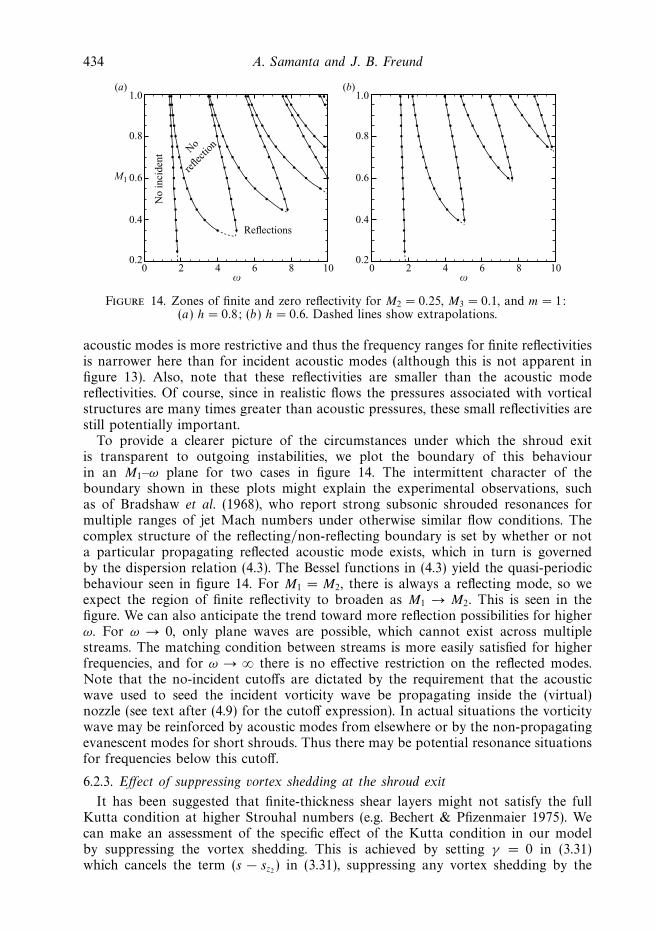
0 2 4ω ω

6 8 100.2

0.4

0.6

0.8

1.0

0.2

0.4

0.6

0.8

1.0(a) (b)

M1

No

reflec

tion

No

inci

dent

Reflections

0 2 4 6 8 10

Figure 14. Zones of finite and zero reflectivity for M2 = 0.25, M3 = 0.1, and m = 1:(a) h = 0.8; (b) h = 0.6. Dashed lines show extrapolations.

acoustic modes is more restrictive and thus the frequency ranges for finite reflectivitiesis narrower here than for incident acoustic modes (although this is not apparent infigure 13). Also, note that these reflectivities are smaller than the acoustic modereflectivities. Of course, since in realistic flows the pressures associated with vorticalstructures are many times greater than acoustic pressures, these small reflectivities arestill potentially important.

To provide a clearer picture of the circumstances under which the shroud exitis transparent to outgoing instabilities, we plot the boundary of this behaviourin an M1–ω plane for two cases in figure 14. The intermittent character of theboundary shown in these plots might explain the experimental observations, suchas of Bradshaw et al. (1968), who report strong subsonic shrouded resonances formultiple ranges of jet Mach numbers under otherwise similar flow conditions. Thecomplex structure of the reflecting/non-reflecting boundary is set by whether or nota particular propagating reflected acoustic mode exists, which in turn is governedby the dispersion relation (4.3). The Bessel functions in (4.3) yield the quasi-periodicbehaviour seen in figure 14. For M1 = M2, there is always a reflecting mode, so weexpect the region of finite reflectivity to broaden as M1 → M2. This is seen in thefigure. We can also anticipate the trend toward more reflection possibilities for higherω. For ω → 0, only plane waves are possible, which cannot exist across multiplestreams. The matching condition between streams is more easily satisfied for higherfrequencies, and for ω → ∞ there is no effective restriction on the reflected modes.Note that the no-incident cutoffs are dictated by the requirement that the acousticwave used to seed the incident vorticity wave be propagating inside the (virtual)nozzle (see text after (4.9) for the cutoff expression). In actual situations the vorticitywave may be reinforced by acoustic modes from elsewhere or by the non-propagatingevanescent modes for short shrouds. Thus there may be potential resonance situationsfor frequencies below this cutoff.

6.2.3. Effect of suppressing vortex shedding at the shroud exit

It has been suggested that finite-thickness shear layers might not satisfy the fullKutta condition at higher Strouhal numbers (e.g. Bechert & Pfizenmaier 1975). Wecan make an assessment of the specific effect of the Kutta condition in our modelby suppressing the vortex shedding. This is achieved by setting γ = 0 in (3.31)which cancels the term (s − sz2

) in (3.31), suppressing any vortex shedding by the


0 1 2 3ω ω

4 50.2

0.4

0.6

0.8

1.0

1.2

0.4

0.3

0.2

0.1

(a) (b)R

mn1

Rmv1

0 1 2 3 4 5

Figure 15. Effect of the Kutta condition on reflectivity for r > h: (a) incident acousticmodes and (b) incident vorticity modes with the full Kutta condition γ = 1 (thick lines) andsuppressed vortex shedding γ = 0 (thin lines). Other parameters are same as in figures 11and 13.

outer vortex sheet. Figure 15 compares the no-vorticity solutions with the full Kuttacondition solutions obtained previously. Suppressing vortex shedding is known toincrease radiation to the far field (Gabard & Astley 2006; Demir & Rienstra 2007).Here it is seen to increase reflectivities. The other interesting aspect of note here is thatfor incident acoustic modes reducing |γ | has more effect on reflectivities for higher ω,unlike acoustic radiation which is affected more at lower frequencies (Rienstra 1983).In contrast, incident vorticity mode reflectivities seem to be more affected at lower ω.

7. ConclusionsThe main result of this study is the reflectivity of vorticity waves back into the

shroud as acoustic modes. These reflectivities are lower than the correspondingreflectivities of outgoing acoustic modes, but the vorticity waves would be expectedto contain many times more energy in a turbulent jet, so these small reflectivitiesare potentially important. The most notable aspect of these reflectivities are thebands in M1–ω coordinates for which there is no reflection. This switch over betweenreflecting and transparent behaviour of the shroud exit might explain the sensitivitiesof observed howling resonances to Mach numbers (Bradshaw et al. 1968). For jetdiameters larger than about half the shroud diameter, these transparent conditionsseem to become prevalent.

The analysis here provides an indication of when a strong feedback loop might existinside the shroud which, however, does not necessarily mean resonance. An obviousextension of this study would be to couple the nozzle of the auxiliary problem of § 4.2with the shroud exit analysis and seek to find resonance conditions. The nozzle,although used to seed the vorticity wave, has not been considered further in theanalysis. The reflected acoustic modes travel upstream and should undergo the modeconversion of acoustic to vortical at the nozzle lip at the given frequency. It wouldalso be of interest to consider extension to supersonic flow conditions for whichresonances are also observed.

Financial support for this work has been provided by AFOSR through grantnumber FA 9550-05-1-0215.


Appendix. Numerical proceduresA.1. Kernel split functions and contour integrals

The kernel (3.22) appears to defy explicit factorization, so K̃+(s) is evaluated usingthe general factorization formula (e.g. Noble 1988):

log K̃+(s) = − 1

2πi

∫C

log[K(σ )/U (σ )]

σ − sdσ, (A 1)

where C is the integration path from −∞ + 0i to ∞ − 0i in S, similar but distinct fromΓ . C must lie above Γ . K̃−(s) is then obtained from (3.23). The factor U (σ ) in (A 1)is from (3.24) and thus removes the instability zeros and pole for the incident acousticcase, so C does not need to be deformed to account for them. For the incidentvorticity case, however, for reasons discussed in § 3.3, U (σ ) is given by (3.25). In thiscase, C must be deformed around both sz1

and sp . The point where C crosses thereal axis has to be carefully chosen to preserve analytic continuity (see the discussionafter (3.30)). Also, a large number of acoustic zeros and poles lie on the real axisnear the origin of the complex plane where the kernel integration is done. This wouldput severe demands upon the adaptive quadrature routines were C to pass near tothem, so C is deformed in the same way as Γ in figure 4(b). The limits for the kernelintegrals are taken such that the contribution of the integrand becomes negligiblebeyond the limits. An adaptive quadrature scheme using the trapezoidal rule has beenused to compute the kernel integrals. It was also confirmed that K̃(s) = K(s)/U (s)in (A 1) does not cross the negative real axis on C, which is a condition that must besatisfied (see Rienstra 2007).

The inverse transform integrals over Γ are only computed for near-field solutions of§ 5. Apart from Γ being similar to C, but lying below, the inversion integrations needto be computed over much smaller limits since the inversion integrand contributionfalls much faster with increasing |s| along Γ . The kernel integrations need to becomputed only once and then the inversion integrals may be computed for any(r, z) pair (see (3.32), (3.35)). It is less computationally expensive here to computethe inversion integrals at a fixed set of points without adaptive refinement and,accordingly, a simple quadrature scheme is used to compute it.

A.2. Kernel approximations

The special functions are computed using standard routines but extra care is neededfor certain ranges of arguments. Computation of (3.22), for example, requires specialconsideration of two factors:

K1 =H(1)

m (λ2ω) + R(s)Jm(λ2ω)

H(1)′m (λ2ω) + R(s)J′

m(λ2ω)and K2 =

H(1)m (λ3ω)

H(1)′m (λ3ω)

. (A 2)

For arguments z with large imaginary part, Bessel functions behave like exp (|Im(z)|),while the Hankel functions behave as exp (iz). The primary requirement is to use scaledfunctions which compensate for these behaviours. However, for very large arguments,when the round-off errors of the denominators of (A 2) become significant, theasymptotic forms for large |λpω|, p = 1, 2, 3,

K1 ≈ i and K2 ≈ 8λ3ω + 4im2 − i

8iλ3ω − 4m2 − 3, (A 3)

are used.


A.3. Reflectivity computations

Computations of reflectivity coefficients using (6.16) are relatively straightforward andless expensive, since as in the § 5 computations no inverse transform is necessary. Thekernel integrals, however, appear in the determination of ξ̂+(μ−

ml) (see (3.30)), where

the split kernels K̂−(μ+mn) and K̂+(μ−

ml) need to be found using the procedures of§ A.1, but only at μ+

mn and μ+ml , respectively. This allows reflectivities to be computed

over ranges of ω as presented in § 6.2 with relatively little computation time.

REFERENCES

Bechert, D. & Pfizenmaier, E. 1975 Optical compensation measurements on the unsteady exitcondition at a nozzle discharge edge. J. Fluid Mech. 71, 123–144.

Bradshaw, P., Flintoff, J. L. & Middleton, D. 1968 Unexplained scale effects in ejector shroud“howling”. J. Sound Vib. 7, 183–190.

Carrier, G. 1956 Sound transmission from a tube with flow. Q. Appl. Maths 13, 457–461.

Crighton, D. G. 1972a Radiation properties of the semi-infinite vortex sheet. Proc. R. Soc. Lond.A 330, 185–198.

Crighton, D. G. 1972b The excess noise fields of subsonic jets. J. Fluid Mech. 56, 683–694.

Crighton, D. G. 1992 The jet edge-tone feedback cycle; linear theory for the operating stages.J. Fluid Mech. 234, 361–391.

Crighton, D. G. & Leppington, F. G. 1974 Radiation properties of the semi-infinite vortex sheet:The initial-value problem. J. Fluid Mech. 64, 393–414.

Crow, S. C. & Champagne, F. H. 1971 Orderly structure in jet turbulence. J. Fluid Mech. 48,547–591.

Demir, A. & Rienstra, S. W. 2007 Sound radiation from a buried nozzle with jet and bypass flow.ICSV14 Paper 449. Cairns.

Gabard, G. & Astley, R. J. 2006 Theoretical model for sound radiation from annular jet pipes:far- and near-field solutions. J. Fluid Mech. 549, 315–341.

Gaster, M., Kit, E. & Wygnanski, I. 1985 Large-scale structures in a forced turbulent mixinglayer. J. Fluid Mech. 150, 23–39.

Heaton, C. J. & Peake, N. 2005 Acoustic scattering in a duct with mean swirling flow. J. FluidMech. 540, 189–220.

Homicz, G. F. & Lordi, J. A. 1975 A note on the radiative directivity patterns of duct acousticmodes. J. Sound Vib. 41, 283–290.

Howe, M. S. 1979 Attenuation of sound in a low Mach number nozzle flow. J. Fluid Mech. 91,209–229.

Howe, M. S. 1987 Self-excited oscillation in jet engine test cells. J. Fluids Struct. 1, 121–148.

Jones, D. S. & Morgan, J. D. 1974 A linear model of a finite amplitude Helmholtz instability. Proc.R. Soc. Lond A 338, 17–41.

Jones, R. R. III & Lazalier, G. R. 1992 The acoustic response of altitude test facility exhaust systemsto axisymmetric and two-dimensional turbine engine exhaust plumes. In DGLR/AIAA 14thAeroacoustics Conference, Eurogress Center, Auchen, Germany , DGLR-Bericht 92-03 , vol. II.

Lee, B. H. K. & Jones, D. J. 1973 Transmission of upstream sound through a subsonic jet. AIAAPaper 73-630.

Levine, H. & Schwinger, J. 1948 On the radiation of sound from an unflanged circular pipe. Phys.Rev. 73, 383–406.

Mani, R. 1973 Refraction of acoustic duct waveguide modes by exhaust jets. Q. Appl. Maths 30,501–520.

Massey, K. C., Ahuja, K. K., Jones, R. R. III & Tam, C. K. W. 1994 Screech tones of supersonicheated free jets. AIAA Paper 93-0141.

Morgan, J. D. 1974 The interaction of sound with a semi-infinite vortex sheet. Q. J. Mech. Appl.Maths 27, 465–487.

Munt, R. M. 1977 The interaction of sound with subsonic jet issuing from a semi-infinite cylindricalpipe. J. Fluid Mech. 83, 609–640.


Munt, R. M. 1990 Acoustic transmission properties of a jet pipe with subsonic jet flow: I. The coldjet reflection coefficient. J. Sound Vib. 142, 413–436.

Noble, B. 1988 Methods based on the Wiener-Hopf technique, 2nd edn. Chelsea.

Orszag, S. A. & Crow, S. C. 1970 Instability of a vortex sheet leaving a semi-infinite plate. Stud.Appl. Maths 49, 167–181.

Pinker, R. A. & Bryce, W. D. 1976 The radiation of plane wave duct noise from a jet exhaust,statically and in flight. AIAA Paper 76-581.

Ridders, C. J. F. 1982 Accurate computation of f ′(x) and f ′(x)f ′′(x). Adv. Engng Softw. 4, 75–76.

Rienstra, S. W. 1983 A small Strouhal number analysis for acoustic wave-jet flow-pipe interaction.J. Sound Vib. 86, 539–556.

Rienstra, S. W. 1984 Acoustic radiation from a semi-infinite annular duct in a uniform subsonicmean flow. J. Sound Vib. 94, 267–288.

Rienstra, S. W. 2007 Acoustic scattering at a hard–soft lining transition in a flow duct. J. EngngMaths 59, 451–475.

Samanta, A. 2008 Finite-wavelength scattering of incident vorticity and acoustic waves at ashrouded-jet exit. PhD thesis, University of Illinois at Urbana-Champaign.

Savkar, S. D. 1975 Radiation of cylindrical duct acoustic modes with flow mismatch. J. Sound Vib.42, 363–386.

Sebourn, C. L. & Shope, F. L. 2005 Research summary on the AEDC ASTF C-2 aeroacousticresonance phenomenon. AIAA Paper 2005-2932.

Strange, P. J. R. & Crighton, D. G. 1983 Spinning modes on axisymmetric jets. Part 1. J. FluidMech. 134, 231–245.

Suzuki, T. & Colonius, T. 2006 Instability waves in a subsonic round jet detected using a near-fieldphased microphone array. J. Fluid Mech. 565, 197–226.

Tam, C. K. W., Ahuja, K. K. & Jones, R. R. III 1994 Screech tones from free and ducted supersonicjets. AIAA J. 32, 917–922.

Taylor, M. V., Crighton, D. G. & Cargill, A. M. 1993 The low frequency aeroacoustics of buriednozzle systems. J. Sound Vib. 163, 493–526.

Veitch, B. & Peake, N. 2007 Models for acoustic propagation through turbofan exhaust flows.AIAA Paper 2007-3543.

Veitch, B. & Peake, N. 2008 Acoustic propagation and scattering in the exhaust flow from coaxialcylinders. J. Fluid Mech. (in press).

finite-wavelength scattering of incident vorticity and...

Documents