fire resistance of materials & structures - analysing the concrete structure

Fire Resistance of Materials & Structures 4th Homework – Concrete structrue

Date of Submission

2016

Submitted by

Seyed Mohammad Sadegh Mousavi

836 154

Submitted to

Prof. R. Felicetti

Prof. P. G. Gambarova

Dr. P. Bamonte

Structural Assessment & Residual Bearing

Capacity, Fire & Blast Safety

Civil Engineering for Risk Mitigation

Politecnico di Milano

[ 4 t h H o m e w o r k - C o n c r e t e S t r u c t u r e ]

of 29

Politecnico di Milano – Lecco Campus


Prof. R. Felicetti & Prof. P. G. Gambarova & Dr. P. Bamonte

Seyed Mohammad Sadegh Mousavi (836154)

Fire Resistance of Materials and Structures Prof. R. Felicetti, Prof. P.G. Gambarova and Dr. P. Bamonte

4th Homework - Concrete structure

The figure below shows the plan of a library room (see Homework 2), whose structural elements are to

be checked (in terms of bearing capacity, R criterion) in fire conditions. The dimensions of the room are

given in centimeters; the height of the room is 3.50 m.

The materials characteristics of the structural elements at room temperature are the following:

Concrete compressive strength: fck = 30 MPa

Yield stress of the reinforcing steel: fyk = 500 MPa

The thermal properties (conductivity, specific heat, and density) of the concrete are given in the Eurocode 2

(EN 1992-1-2); assume the lower bound of thermal conductivity and 0% moisture for F even, upper bound

and 1.5% for F odd (F = 3rd letter of the first name).

The two spans are L1 = 4 - L/100 and L2 = 4 + L/100 (in meters, L = 3rd letter of the last name). The room is

subjected to the following loads:

permanent load: Gk = 7.00 kN/m2

variable load: Qk = 2.00 kN/m2

The beam has a rectangular section, and its structural scheme is shown on the right-end side of the picture.

The center support represents the central column. The total depth of the section is h1 = 24 cm; the net

cover to the bars is 30 mm.

of 29





(a) Design the critical beam sections at room temperature, by determining the reinforcement, and

then evaluate the fire endurance of the beam (with reference to the fire scenario studied in

Homework 2) by means of the 500°C isotherm method. Both the static and the kinematic

approach should be applied, and the differences between the two should be commented.

To ensure the ductility requirements at room temperature, the relative depth of the compression

zone must not be larger than x/d = 0.40.

Optional

Let us assume that the central column is removed: the new section and the corresponding structural scheme

are indicated in the figure below. The total depth h2 becomes 60 cm.

(b) Repeat step (a) for the new section and structural scheme, and comment on the possible

interaction with the boundaries.

L = 21 (U)

𝐿1 = 4 −𝐿

100= 3.79 𝑚

𝐿2 = 4 +𝐿

100= 4.21 𝑚

of 29





The fire used in this case is the parametric fire in EuroCode 1. So concrete strength is 30 Mpa and steel

yield strength is 500 Mpa. On the other hand, thermal properties of the material are based on the EuroCode

2. Consideri other parameters such as thermal conductivity and specific heat, the upper bound and the

condition according to 1.5 % moisture content are considered respectively.

Figure 1 – General Scheme of the Beams

Loads

Permanent: Gk = 7.00 kN/m2

Variable: Qk = 2.00 kN/m2

The design of the beam is carried out based on static and kinematic mechanisms and for each condition

the fire endurance is determined. The temperature evolution within the member is modelled using

ABAQUS software and the decay of the bending moment resistance of the section is calculated based on

a 500 ̊C isotherm method.

Design of the critical beam sections at room temperature

(ULS) – Ultimate Moments Computations

Floor Loads

𝑃𝑈𝐿𝑆 = 𝛾𝐺𝐺𝑘 + 𝛾𝑄𝑄𝑘 = 1.35 × 7 (𝐾𝑁

𝑚2) + 1.5 × 2 (

𝐾𝑁

𝑚2) = 12.45 (

𝐾𝑁

𝑚2)

Contribution (Effective) width: we assume bending continuity between the two bays of the slab, this width

is: 2 ×5

8× 6 = 7.5 𝑚

Figure 2 – Bay width

Internal Forces (ULS)

𝑔𝑈𝐿𝑆 = 12.45 × 7.5 = 93.375 (𝐾𝑁

𝑚)

𝑞𝑈𝐿𝑆 = (1.5 × 2) × 7.5 = 22.5 (𝐾𝑁

𝑚)

of 29





For designing the beam at room temperature, 3 critical combinations were considered:

1- Negative bending moment at the intermediate soppurt.

2- Max positive bending moment in the left span.

3- Max positive bending moment in the right span.

For reach to that aim, 3 different load cases were considere by selecting the load spans with variable loads

as following:

Figure 3 – Bending Moment Diagram Scheme

1st Combination – Negative Bending moment at the intermediate soppurt

Figure 4 – Max loaded at the intermediate soppurt

3 33 31 2

,11 2

93.375 3.79 93.375 4.21188.29 .

8( ) 8 3.79 4.21Ed

wL wLM KN m

L L

,1 11

1

188.29 93.375 3.79 127.262 3.79 2

EdM wL

R KNL

11

127.261.36

93.375

Rx

w

of 29





2nd Combination – Max Loaded on the left side

Figure 5 – Max loaded on the left side

2 21

1 1,2, 1

93.375 1.36127.26 1.36 86.72 .

2 2Ed x

wxM R x KN m

,1 23

2

188.29 93.375 4.21

4.21 2151.83

2Ed

M wLR KN

L

3rd Combination – Max Loaded on the right side

Figure 6 – Max Loaded on the right side

32

151.831.63

93.375

Rx

w

2 22

3 2,3, 2

93.375 1.63151.83 1.63 123.44 .

2 2Ed x

wxM R x KN m

Sections Combinations 𝑴𝑬𝒅(𝑲𝑵. 𝒎)

Support Combination 1 188.29

Left Span Combination 2 86.72

Right Span Combination 3 123.44

Applied Design Moment (at the support)

188.29 .Ed

M KN m

of 29





Materials (Concrete + Steel) used and their properties:

Concrete

The characteristic compressive strength = 𝒇𝒄𝒌 = 𝟑𝟎 𝑴𝑷𝒂 = 30 (𝑁

𝑚𝑚2)

The design value of compressive strength

𝒇𝒄𝒅 = 𝜶 ×𝒇𝒄𝒌

𝜸𝒄= 0.85 ×

30

1.6= 15.94 𝑀𝑃𝑎 = 𝟏𝟓. 𝟗𝟒 (

𝑁

𝑚𝑚2)

- The ultimate strain of concrete eCU=0.0035

- The strength reduction value a= 0.85

- The material factor of safety for concrete gc=1.6

Steel

The characteristic yield strength = 𝒇𝒚𝒌 = 𝟓𝟎𝟎 𝑴𝑷𝒂 = 500 (𝑁

𝑚𝑚2)

The design value of compressive strength

𝒇𝒚𝒅 =𝒇𝒚𝒌

𝜸𝒔=

500

1.15= 437.78 𝑀𝑃𝑎 = 437.78 (

𝑁

𝑚𝑚2)

- The elastic Modulus Es=200000 (𝑁

𝑚𝑚2)

- The ultimate strain of steel eCU=0.01

- The yield strain of steel 𝜺𝒚𝒅 =𝒇𝒚𝒅

𝑬𝒔= 0.00217

- The material factor of safety for steel reinforcement gs=1.15

The cross section geometric

Figure 7 – Cross Section Details

The Design Procedure

1st Assumption of computation of amount of longitudinal reinforcement in Tension & Compression zones

by the following formulas:

'

0.9

0.5

Eds

yd

s s

MA

f d

A A

of 29





Figure 8 – Assumptions of Reinforcements

Ductility Check

Basically the structures show 2 type of failures (Ductile & Brittle), and in case of safety and clear warming

prior to collapse by increased deflection, curvature & cracking, ductile failure should be considered in

design phase and must be preventing the brittle failure.The following figure (Fig. 5) shows 6 failure fields

and each 7 limit lines represents different limit states for the section.

Figure 9 – Failure Fields

The procedure was based on considering the maximum exploitation of the cross section by assuming the

ultimate steel strain (Point A, εs = εsu = 0.01), and the maximum compressive concrete strain (Point B, εc

= εcu = 0.0035) are reached and Piont C shows the yield strain of steel. For deisgning the beam, ductile

behavior is an important criteria that should be respect and so can fall into fields 2 or 3. On the other

hand, in field 2, the bottom reinforcement reaches the ultimate strain & failure is expected to happen in

ductile method. In field 3, concrete does reach ultimate strain, but steel has yielded and it is in the plastic

range. As a result, gradually ductile failure is to be expected.

According to the depth of the compressive zone, ductility requirement: 𝑦𝑛

𝑑= 𝜉 ≤ 0.4

Med (Soppurt)= 188.29

As= 22.91 25.4 10 Φ 18

As'= 11.46 12.7 5 Φ 18

Bars

Med (Left)= 86.72

As= 10.55 12.7 5 Φ 18

As'= 5.28 7.62 3 Φ 18

Bars

Med (Right)= 123.44

As= 15.02 15.24 6 Φ 18

As'= 7.51 10.16 4 Φ 18

Bars

Needed Selected

of 29





Due to this fact that tensile strength of concrete is neglected, resistance of concrete in tension zone is

ignored. Only considered the comprssion force developed in concrete. Depth of compressive zone should

be ≤ 0.4 d.

1st case – Cross section at span

Figure 10 – Cross Section at Span

2nd Case – Cross section at intermediate soppurt

Figure 11 – Cross Section at intermediate soppurt

According of the depth of compression, the position of Neutral Axis will be obtained. And also respecting

the ductility requirement, it maybe concluded at intermediate soppurt works in Field 3 while span secions

work in Field 2.

Failue Field 2 for the 1st case:

𝟎 < 𝝃 ≤ 𝟎. 𝟐𝟓𝟗𝒅

Concrete and also bottom reinforcement reach max strain, thus max exploitation of section resource is

achieved.

εcu = 0.0035, εsu = 0.01, 𝜺𝒚𝒅 =𝒇𝒚𝒅

𝑬𝒔

Factor for the equivalent stress block (β) 𝛃 = (𝟏. 𝟔 × 𝟎. 𝟖�̅�𝒄) × �̅�𝒄

Factor for the position of the concrete force (k) 𝒌 = (𝟎. 𝟑𝟑 + 𝟎. 𝟎𝟕)�̅�𝒄

�̅�𝒄 =𝜺𝒄

𝜺𝒄𝒖

By computation of this, we can know the ductile and brittle behavior, so it is important procedure to

determine the type of failure mechanism.

of 29





Strain Compatibility equations, for calculation of Neutral axis position in field 2:

0 < 𝜉 ≤ 0.259 𝑑

. 0.00350.259

0.0035 0.01cu su cu

nn n cu su

d dy d

y d y

1csu

,

.( )'

1su

s

in field 3:

𝟎. 𝟐𝟓𝟗 𝒅 < 𝝃 ≤ 𝟎. 𝟔𝟓𝟐 𝒅

0.00187

0.00350.652

0.0035ydcu

nn n yd

dy d

y d y

Max strain in conrete is reached at Point B:

εcu = 0.0035, εsu = 0.01, 𝜺𝒚𝒅 =𝒇𝒚𝒅

𝑬𝒔

β = 0.8, k = 0.4

Strain Compatibility equations, for calculation of Neutral axis position:

.(1 )cu s cusd d d

' .( )'

'cu s cu

sd d d

Concrete Cover Coefficient:

'

d

d

Stresses can be obtained used σ – ε constitutive models:

𝛔𝒄 = 𝒇𝒄𝒅 = 𝜶 ×𝒇𝒄𝒌

𝜸𝒄= 0.85 ×

30

1.6= 15.94 𝑀𝑃𝑎 = 15.94 (

𝑁

𝑚𝑚2)

𝛔𝒔 = 𝒇𝒚𝒅 =𝒇𝒚𝒌

𝜸𝒔=

500

1.15= 437.78 𝑀𝑃𝑎 = 437.78 (

𝑁

𝑚𝑚2)

𝛔′𝒔 = 𝐄𝒔 𝛆′𝒔

Concrete & reinforcement forces:

Concrete compression force C = - σcd × β × yn × b

Compression steel force C’ = - σs’ × As‘

Tension steel force T = σs × As

of 29





2 Equilibrium conditions can be imposed:

Force Equlibrium

Rotation Equilibrium

Aim: Finding the value of inside ξ the ranges of each field (2 & 3) that will verify force equlibrium

condirion & checking MEd ≤ MRd

Using Excelsheets for reaching to this aim.

1st Condition – Soppurt (3rd Failure Field)

2nd Condition – Left Span (2nd Failure Field)

3rd Condition – Right Span (2nd Failure Field)

Σ F = C + C’ + T = 0

MRd = σc + β × yn × b × (d – k × yn) + σs’ × As‘× (d – d’)

of 29





Figure 12 – Bending moment & force equlibriums check of the section for different situations

As we can see on the top figure (Fig. 12), the moment equlibriums of different cases were satisfied, but,

with those positions of N.A that we considered the max values with respect to the boundary conditions of

2 fields, the force equlibriums were not satisfied and those values were negative which replies the

compression parts are too much, and so for satisfying the force equlibrium, the positions of N.A should

be changed, reduced and repeating the procedueres. What’s more, according to the force equlibrium is

very sensitive about the changing of position of N.A, the Solver add-in of excel used to find the exact

positions of N.A in different cases, then SF=0, as you can see in the next figure (Fig. 13).

fck= 30 N/mm2 fck= 30 N/mm2 fck= 30 N/mm2

fyk= 500 N/mm2 fyk= 500 N/mm2 fyk= 500 N/mm2

Es= 200000 N/mm2 Es= 200000 N/mm2 Es= 200000 N/mm2

Ecm= 32000 N/mm2 Ecm= 32000 N/mm2 Ecm= 32000 N/mm2

εcu= 0.0035 εcu= 0.0035 εcu= 0.0035

εsu= 0.01 εsu= 0.01 εsu= 0.01

γc= 1.5 γc= 1.5 γc= 1.5

γs= 1.15 γs= 1.15 γs= 1.15

h= 240 mm h= 240 mm h= 240 mm

d'= 30 mm d'= 30 mm d'= 30 mm

d= 210 mm d= 210 mm d= 210 mm

b= 600 mm b= 600 mm b= 600 mm

δ= 0.1429 mm δ= 0.1429 mm δ= 0.1429 mm

As= 2540 mm2 As= 1270 mm2 As= 1524 mm2

As'= 1270 mm2 As'= 762 mm2 As'= 1016 mm2

fcd= 15.94 N/mm2 fcd= 15.94 N/mm2 fcd= 15.94 N/mm2

fyd= 434.78 N/mm2 fyd= 434.78 N/mm2 fyd= 434.78 N/mm2

εyd= 0.0021739 εyd= 0.0021739 εyd= 0.0021739

ξ max(f.3)= 0.652 ξ max(f.2)= 0.259 ξ max(f.2)= 0.259

εs= 0.006329604 εc= 0.003058824 εc= 0.0032316

εs'= 0.0020958 N/mm2 εs'= 0.0011933 N/mm2 εs'= 0.001341 N/mm2

ε_cu= 1.808 ε_cu= 0.874 ε_cu= 0.9233024

σc= 15.94 N/mm2 σc= 15.94 N/mm2 σc= 15.94 N/mm2

σs= 434.78 N/mm2 σs= 434.78 N/mm2 σs= 434.78 N/mm2

σs'= 419.154 σs'= 238.655 σs'= 268.267

k= 0.4 k= 0.35 k= 0.3693210

β= 0.8 β= 0.79 β= 0.7952940

yn= 136.92 mm yn= 54.39 yn= 54.39

MRd= 258.41 KN/m MRd= 110.94 KN/m MRd= 127.62 KN/m

MEd= 188.29 KN/m MEd= 86.720 KN/m MEd= 123.44 KN/m

Σf=0 -475415.972 Σf=0 -39154.03999 Σf=0 -23586.62250

Moment EQ Check

Force EQ Check

SAFE MEd ≤ MRd

3rd Cond - Right Span (Field 2)

Material Properties

Material Factors

Cross Section Geometric

Assumed Bars

SAFE MEd ≤ MRd

Moment EQ Check

Force EQ Check Force EQ Check

1st Cond - Support (Field 3)

SAFE MEd ≤ MRd

2nd Cond - Left Span (Field 2)

Material Properties

Material Factors


Assumed Bars

Material Properties

Material Factors


Assumed Bars

Moment EQ Check

of 29





Figure 13 – The Final Position of N.A & Force Equlibrium Check

The new positions of N.A:

ξ1 (Field 3) = 0.356067244109769

ξ2 (Field 2) = 0.234234241633019

ξ3 (Field 2) = 0.244231128360258

Eventually, all the values of ξ < 0.4 that the ductility of section is satisfied.

Check the minimum reinforcement ratio

According to EN1992-1-1 6.2.2, 𝜌𝑤 should be not less than 𝜌𝑤,𝑚𝑖𝑛

𝝆𝒘,𝒎𝒊𝒏 =𝟎. 𝟎𝟖√𝒇𝒄𝒌

𝒇𝒚𝒌= 0.00087

,Soppurt

25400.02

210 600w

,

,Left

12700.01

210 600w

,

,Right

15240.012

210 600w

So, All the reinforcement ratios satisfied the requirement.

Thermal Analysis

Thermal analysis was done by the ABAQUS with neglecting the reinforcements in the model due this fact

the effects of it are very small and with respect to the volume of the concrete is negligible and also it was

demonstrated that the temperature in the centroid of the bars will not change.

Concrete properties

Density (ρ) - weight per unit mass of the material (kg/m3)

According to the Eurocode 2 Part 1&2 (2004)

𝜌(𝑡) = 𝜌(20 ℃) 𝐹𝑜𝑟 20 ℃ ≤ 𝑡 ≤ 115 ℃

𝜌(𝑡) = 𝜌(20 ℃) ∙ (1 −0.02(𝑡 − 115)

85) 𝐹𝑜𝑟 115 ℃ < 𝑡 ≤ 200 ℃

𝜌(𝑡) = 𝜌(20 ℃) ∙ (0.98 −0.03(𝑡 − 200)

200) 𝐹𝑜𝑟 200 ℃ < 𝑡 ≤ 400 ℃

𝜌(𝑡) = 𝜌(20 ℃) ∙ (0.95 −0.07(𝑡 − 400)

800) 𝐹𝑜𝑟 400 ℃ < 𝑡 ≤ 1200 ℃

The following graph represent the concrete density with respect to the equations for different

temperatures that mentioned in the previous page and plotted in excel code.

ξ max(f.3)= 0.652 ξ max(f.2)= 0.259 ξ max(f.2)= 0.259

ξ (f.3)= 0.3560672441 ξ (f.2)= 0.2342342416 ξ (f.2)= 0.2442311284

Σf=0 0.00000 Σf=0 0.00000 Σf=0 0.00000

Force EQ Check Force EQ Check Force EQ Check

of 29





Figure 14 – Concrete Density graph

Specific Heat (c) - amount of heat required to heat unit mass of the material by one degree (J/kg.K).

According to the Eurocode 2 Part 1&2 (2004)

𝑐𝑝(𝑡) = 900 (𝐽

𝐾𝑔 𝐾⁄ ) 𝐹𝑜𝑟 20 ℃ ≤ 𝑡 ≤ 100 ℃

𝑐𝑝(𝑡) = 900 + (𝑡 − 100) (𝐽

𝐾𝑔 𝐾⁄ ) 𝐹𝑜𝑟 100 ℃ < 𝑡 ≤ 200 ℃

𝑐𝑝(𝑡) = 1000 +𝑡 − 200

2 (

𝐽𝐾𝑔 𝐾⁄ ) 𝐹𝑜𝑟 200 ℃ < 𝑡 ≤ 400 ℃

𝑐𝑝(𝑡) = 1100 (𝐽

𝐾𝑔 𝐾⁄ ) 𝐹𝑜𝑟 400 ℃ < 𝑡 ≤ 1200 ℃

Concrete is assumed with 0% of moisture. Because according to the discussion during the class, if there

is moist inside the concrete the graph of the temperature versus time is different. But in the following

graph the increasing in the trend happened due to vaporization of the water that called latent heat.

2075

2125

2175

2225

2275

2325

2375

2425

20 150 280 410 540 670 800 930 1060 1190

DEN

SITY

(K

G/M

3)

TEMPERATURE (℃)

CONCRETE - DENSITY

of 29





Figure 15 – Concrete Specific Heat graph

Conductivity (λ) - rate of heat transferred per unit thickness of material per unit temperature difference

(W/m.K). EN1992-1-2 proposes lower and upper limit of thermal conductivity. Regarding the maximum

and minimum formulas for thermal conductivity in the Eurocode 2, the average value of these formulas

considered as a reference value for the concrete thermal conductivity in the ABAQUS code.

According to the Eurocode 2 Part 1-2 (2004) – MAX & MIN Conductivity

𝜆𝑐𝑚𝑎𝑥(𝑡) = 2 − 0.2451 (

𝑡

100) + 0.0107 (

𝑡

100)

2

𝜆𝑐𝑚𝑖𝑛(𝑡) = 1.36 − 0.136 (

𝑡

100) + 0.0057 (

𝑡

100)

2

Figure 16 – Concrete Conductivity graph (Average Value)

850

900

950

1000

1050

1100

1150

20 150 280 410 540 670 800 930 1060 1190

SPEC

IFIC

HEA

T (J

/KG

K)

TEMPERATURE (℃)

CONCRETE - SPECIF IC HEAT

0.2

0.6

1.0

1.4

1.8

20 145 270 395 520 645 770 895 1020 1145

CO

ND

UC

TIV

ITY

(W/M

K)

TEMPERATURE (C)

C O N C R E T E - T H E R M A L C O N D U C T I V I T Y ( A V E R A G E V A L U E )

of 29





The procedures of the cross section implementation in the ABAQUS is almost the same as exercise 1 and

we will mentioned the differences in the following. In this case, the Parametric Fire obtained from exercise

2 was used, for the linear temp depending openings.

Figure 17 – Radiation & Convections of the surfaces

Figure 18 – Details of the Radiation & Convections of the Surfaces

of 29





500 °C Isotherm

As you can see in the following table (Fig. 19), the position of 500 °C isotherm was extracted

approximately by defining a vertical path & temperature, was plotted with distance for each 30 min fire

duration. In addtition, the temperature of top & bottom steel reinforcement was found at each 30 minutes

of fire duration, in order to find out the steel properties decay at each step. It worth to mention that the

upper reinforcement had always a temperature less than 130°C. (Fig. 20)

Figure 19 – The temperature distribution among the Cross Section

Figure 20 – Postion of 500°C isotherm for different time & temperatures

Time 30 min 60 min 90 min 120 min 150 min 180 min 210 min 240 min

Distance [m] [°C] [°C] [°C] [°C] [°C] [°C] [°C] [°C]

0 1047.88 1211.54 1255.75 1279.97 1296.15 1303.63 1316.89 1231.19

0.0025 919.742 1127.34 1189.68 1223.69 1246.24 1256.64 1275.15 1206.27

0.005 808 1045.01 1124.11 1167.69 1196.58 1209.87 1233.56 1179.65

0.0075 712.646 966.471 1059.58 1112.14 1147.13 1163.3 1192.14 1151.48

0.01 631.523 893.085 997.161 1057.48 1098.12 1117.02 1150.87 1122.02

0.0125 562.094 825.477 937.696 1004.37 1049.99 1071.35 1109.88 1091.58

0.015 502.173 763.753 881.586 953.332 1003.12 1026.66 1069.42 1060.4

0.0175 450.085 707.608 828.993 904.611 957.875 983.227 1029.74 1028.8

0.02 404.483 656.487 779.986 858.432 914.444 941.319 991.063 997.083

0.0225 364.292 609.916 734.41 814.846 872.985 901.085 953.551 965.462

0.025 328.651 567.414 692.066 773.815 833.549 862.618 917.343 934.191

0.0275 296.885 528.511 652.719 735.248 796.132 825.958 882.499 903.427

0.03 268.442 492.803 616.122 699.016 760.699 791.08 849.076 873.335

0.0325 242.881 459.95 582.032 664.971 727.153 757.959 817.049 844.056

0.035 219.853 429.652 550.234 632.963 695.42 726.498 786.426 815.623

0.0375 199.05 401.641 520.545 602.864 665.38 696.643 757.189 788.118

0.04 180.219 375.709 492.75 574.5 636.935 668.291 729.255 761.584

0.0425 163.297 351.637 466.708 547.76 610.005 641.356 702.595 735.992

0.045 148.196 329.243 442.274 522.529 584.458 615.776 677.146 711.363

0.0475 134.798 308.388 419.296 498.666 560.212 591.446 652.824 687.696

0.05 122.978 288.935 397.674 476.089 537.2 568.282 629.593 664.931

0.0525 112.61 270.755 377.318 454.721 515.321 546.232 607.401 643.055

0.055 103.555 253.743 358.114 434.457 494.491 525.221 586.164 622.055

0.0575 95.6604 237.816 339.964 415.215 474.658 505.166 565.836 601.884

0.06 88.4913 222.894 322.803 396.942 455.767 486.017 546.385 582.488

0.0625 81.9424 208.897 306.571 379.58 437.744 467.734 527.753 563.846

0.065 75.9633 195.756 291.197 363.059 420.528 450.261 509.884 545.941

0.0675 70.5082 183.424 276.618 347.317 404.082 433.539 492.736 528.728

0.07 65.5354 171.889 262.779 332.308 388.374 417.522 476.283 512.165

0.0725 61.0064 161.137 249.638 317.996 373.351 402.183 460.492 496.217

0.075 56.8856 151.143 237.16 304.341 358.969 387.492 445.321 480.87

0.0775 53.1402 141.878 225.304 291.299 345.187 373.405 430.731 466.1

0.08 49.7398 133.312 214.03 278.833 331.975 359.886 416.693 451.875

Concrete temperature

of 29





As a result, the approximate position of 500 °C isotherm and temperatures of the top & bottom

reinforcements are as the following:

Figure 21 – The approcimate position of 500°C isotherm

Figure 22 – The top & Bottom Reinforcements temperatures

Figure 23 – Temp Evolution along the vertical line for different Fire durations

Time 30 min 60 min 90 min 120 min 150 min 180 min 210 min 240 min

x - Distance [cm] 1.5 2.95 3.95 4.75 5.5 5.8 6.5 7.2

574.5 636.935 668.291 729.255 761.584Temp [°C] at Bottom

Reinforcement180.219 375.709 492.75

500°C Isotherm [Approximately]

68.89 81.60 109.09 128.55Temp [°C] at Top

Reinforcement20.04 22.60 32.52 48.87

0

100

200

300

400

500

600

700

800

0 40 80 120 160 200 240

TEM

PER

ATU

RE

[°C

]

TIME [MIN]

Reinforcement Temperature

Top ReinforcementsBottom Reinforcements

0

100

200

300

400

500

600

700

800

900

1000

1100

1200

1300

1400

0 0.03 0.06 0.09 0.12 0.15 0.18 0.21 0.24

Temperature Evolution Through the Vertical Line for Differents Fire Durations

30 min

60 min

90 min

120 min

150 min

180 min

210 min

240 min

500 °C Isotherm

of 29





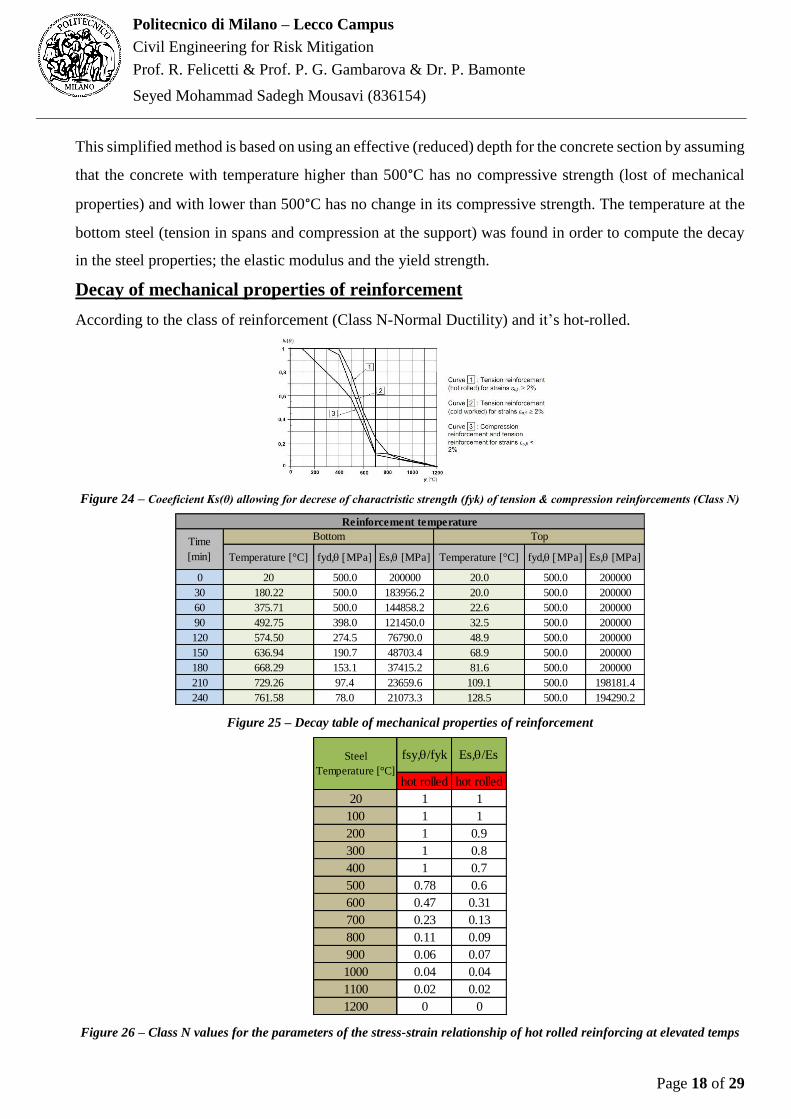
This simplified method is based on using an effective (reduced) depth for the concrete section by assuming

that the concrete with temperature higher than 500°C has no compressive strength (lost of mechanical

properties) and with lower than 500°C has no change in its compressive strength. The temperature at the

bottom steel (tension in spans and compression at the support) was found in order to compute the decay

in the steel properties; the elastic modulus and the yield strength.

Decay of mechanical properties of reinforcement

According to the class of reinforcement (Class N-Normal Ductility) and it’s hot-rolled.

Figure 24 – Coeeficient Ks(θ) allowing for decrese of charactristic strength (fyk) of tension & compression reinforcements (Class N)

Figure 25 – Decay table of mechanical properties of reinforcement

Figure 26 – Class N values for the parameters of the stress-strain relationship of hot rolled reinforcing at elevated temps

Temperature [°C] fyd,q [MPa] Es,q [MPa] Temperature [°C] fyd,q [MPa] Es,q [MPa]

0 20 500.0 200000 20.0 500.0 200000

30 180.22 500.0 183956.2 20.0 500.0 200000

60 375.71 500.0 144858.2 22.6 500.0 200000

90 492.75 398.0 121450.0 32.5 500.0 200000

120 574.50 274.5 76790.0 48.9 500.0 200000

150 636.94 190.7 48703.4 68.9 500.0 200000

180 668.29 153.1 37415.2 81.6 500.0 200000

210 729.26 97.4 23659.6 109.1 500.0 198181.4

240 761.58 78.0 21073.3 128.5 500.0 194290.2

Bottom TopTime

[min]

Reinforcement temperature

hot rolled hot rolled

20 1 1

100 1 1

200 1 0.9

300 1 0.8

400 1 0.7

500 0.78 0.6

600 0.47 0.31

700 0.23 0.13

800 0.11 0.09

900 0.06 0.07

1000 0.04 0.04

1100 0.02 0.02

1200 0 0

fsy,q/fyk Es,q/EsSteel

Temperature [°C]

of 29





Evaluation of the fire endurance of the beam

Bearing capacity of the beam in fire is check by 2 methods:

Static Method

Kinematic Method

With the same concept of the load combinations at room temp, 3 bending moment were computed by

SAP2000 for 3 critical section (Left & Right spans and at the Support)

Sections 𝑴𝑬𝒅(𝑲𝑵. 𝒎)

Support 142.66

Left Span 69.91

Right Span 92.73

Figure 27 – Bending Moments

The Static Method

According to this method, we can compute the resisting bending moment for each section at different time

steps (every 30 minutes) by the same way used for the design at room temperature, but considering the

changes due to the raise in the temperature in the bottom steel properties and in the effective concrete

section. It worth to mention that even if the effective depth is used for the strain compatibility relation and

for the concrete force computation, still the depth used for the deliver arm of the steel reinforcement is

the initial depth. The excel spreadsheet produced and provided in the report computes at each time step,

the location of the neutral axis that satisfies the equilibrium, then computes the resistant moment.

The constant applied bending moments (MEd) are compared with the resistant bending moments (MRd) at

each time step. When the resistant bending moment is less than the applied moment, the failure occurs

according to the static sectional method considered.

Calculations MRd in fire condition at different time step for the section:

of 29





Figure 28 – Resisting bending moment & force equlibrium of Support

Tim

eIn

itialt=

30

min

t= 6

0 m

int=

90

min

t= 1

20

min

t=1

50

min

t=1

80

min

t= 2

10

min

t=2

40

min

fck (N/m

m2)=

3030

3030

3030

3030

30

fyk (N/m

m2)=

500500

500500

500500

500500

500

Es' (N

/mm

2)=200000

200000200000

200000200000

200000200000

200000200000

fcd = α.fck25.5

25.525.5

25.525.5

25.525.5

25.525.5

εcu=0.0035

0.00350.0035

0.00350.0035

0.00350.0035

0.00350.0035

d' (mm

)=30.00

15.000.50

-9.50-17.50

-25.00-28.00

-35.00-42.00

d (mm

)=201

186171.5

161.5153.5

146143

136129

b (mm

)=600

600600

600600

600600

600600

δ (mm

)=0.15

0.080.00

-0.06-0.11

-0.17-0.20

-0.26-0.33

As (m

m2)=

25402540

25402540

25402540

25402540

2540

As' (m

m2)=

12701270

12701270

12701270

12701270

1270

dT=500 [m

m]=

0.0015.00

29.5039.50

47.5055.00

58.0065.00

72.00

d eff=210.00

195.00180.50

170.50162.50

155.00152.00

145.00138.00

T (reinfor.)=

20.00180.22

375.71492.75

574.50636.94

668.29729.26

761.58

fyd,θ=500

500500

398274.50

190.70153.10

97.4078

Es,θ=

200000183956.2

144858.2121450.00

76790.0048703.40

37415.2023659.60

21073.30

ξ =0.3222334305

0.29639874640.3012334264

0.31901259400.4480513227

0.55194727200.5995322262

0.67568819410.7181054793

ξ (Field) = Field 3

Field 3 Field 3

Field 3 Field 3

Field 3 Field 3

Field 3 Field 3

εs' (N/m

m2)=

0.001878850.00254771

0.003466130.00414537

0.004390570.00458582

0.004643080.00483306

0.00508686

σc (N/m

m2)=

25.525.5

25.525.5

25.525.5

25.525.5

25.5

σs (N/m

m2)=

500500

500500

500500

500500

500

σs'=375.77

468.67502.10

503.46337.15

223.34173.72

114.35107.20

k=0.40

0.400.40

0.400.40

0.400.40

0.400.40

β=0.80

0.800.80

0.800.80

0.800.80

0.800.80

yn (mm

)=64.77

55.1351.66

51.5268.78

80.5885.73

91.8992.64

MR

d (K

N.m

)=2

20

.41

21

2.4

12

04

.42

19

8.1

81

79

.28

16

0.7

21

51

.80

13

6.4

61

27

.53

ME

d (K

N.m

)=

Mom

ent E

Q C

heck

SA

FE

ME

d ≤

MR

d

SA

FE

ME

d ≤

MR

d

SA

FE

ME

d ≤

MR

d

SA

FE

ME

d ≤

MR

d

SA

FE

ME

d ≤

MR

d

SA

FE

ME

d ≤

MR

d

SA

FE

ME

d ≤

MR

d

No

t Safe

No

t Safe

Σf=

00

.00

00

00

00

.00

00

00

00

.00

00

00

00

.00

00

00

00

.00

00

00

00

.00

00

00

00

.00

00

00

00

.00

00

00

00

.00

00

00

0

Ele

vate

d T

em

p fo

r the

So

pp

urt (F

ield

3)

14

2.6

6

Force E

Q C

heck

of 29





Figure 29 – Resisting bending moment & force equlibrium of Left Span

Tim

eInitial

t= 30 m

int=

60 min

t= 90 m

int=

120 min

t=150 m

int=

180 min

t= 210 m

int=

240 min

fck (N/m

m2)=

3030

3030

3030

3030

30

fyk (N/m

m2)=

500500

500500

500500

500500

500

ε su0.01

0.010.01

0.010.01

0.010.01

0.010.01

fcd = α.fck25.5

25.525.5

25.525.5

25.525.5

25.525.5

εc=0.002088

0.0021180.002211

0.0020410.001824

0.0016120.001490

0.0012700.001190

εcu=0.0035

0.00350.0035

0.00350.0035

0.00350.0035

0.00350.0035

ε_cu=0.59645

0.605040.63161

0.583140.52101

0.460560.42573

0.362780.33994

d' (mm

)=30

3030

3030

3030

3030

d (mm

)=210

210210

210210

210210

210210

b (mm

)=600

600600

600600

600600

600600

δ (mm

)=0.14286

0.142860.14286

0.142860.14286

0.142860.14286

0.142860.14286

As (m

m2)=

12701270

12701270

12701270

12701270

1270

As' (m

m2)=

762762

762762

762762

762762

762

dT=500 [m

m]=

0.0015.00

29.5039.50

47.5055.00

58.0065.00

72.00

d eff=210.00

195.00180.50

170.50162.50

155.00152.00

145.00138.00

T (reinfor.)=

20.00180.22

375.71492.75

574.50636.94

668.29729.26

761.58

fyd,θ=500

500500

398274.5

190.7153.1

97.478

Es,θ=

200000183956.2

144858.2121450.00

76790.0048703.40

37415.2023659.60

21073.30

ξ =0.1727036512

0.17475732890.1810406031

0.16950308120.1542281813

0.13881855180.1296814707

0.11266700600.1063270059

ξ (Field) = Field 2

Field 2 Field 2

Field 2 Field 2

Field 2 Field 2

Field 2 Field 2

εs' (N/m

m2)=

0.001728190.00182540

0.002109110.00157200

0.00073729-0.00029093

-0.00101600-0.00267959

-0.00343564

σc (N/m

m2)=

25.525.5

25.525.5

25.525.5

25.525.5

25.5

σs (N/m

m2)=

500.0500.0

500.0398.0

274.5190.7

153.197.4

78.0

σs'=345.64

335.79305.52

190.9256.62

-14.17-38.01

-63.40-72.40

k=0.23858

0.242020.25264

0.233260.20840

0.184220.17029

0.145110.13597

β=0.66972

0.675210.69143

0.660980.61645

0.567200.53617

0.475160.45145

yn (mm

)=36.27

36.7038.02

35.6032.39

29.1527.23

23.6622.33

MR

d (KN

.m)=

122.23122.31

122.5098.79

69.8549.82

40.6626.84

21.99

ME

d (KN

.m)=

Mom

ent EQ C

heckSA

FE

ME

d ≤ MR

d SA

FE

ME

d ≤ MR

d SA

FE

ME

d ≤ MR

d SA

FE

ME

d ≤ MR

d N

ot SafeN

ot SafeN

ot SafeN

ot SafeN

ot Safe

Σf=

00.0000000

0.00000000.0000000

0.00000000.0000000

0.00000000.0000000

0.00000000.0000000

Elevated T

emp for the L

eft Span (Field 2)

69.91

Force E

Q C

heck

of 29





Figure 30 – Resisting bending moment & force equlibrium of Right Span

Tim

eIn

itialt=

30

min

t= 6

0 m

int=

90

min

t= 1

20

min

t=1

50

min

t=1

80

min

t= 2

10

min

t=2

40

min

fck (N/m

m2)=

3030

3030

3030

3030

30

fyk (N/m

m2)=

500500

500500

500500

500500

500

ε su0.01

0.010.01

0.010.01

0.010.01

0.010.01

fcd = α

.fck25.5

25.525.5

25.525.5

25.525.5

25.525.5

εc=0.002131

0.0021680.002285

0.0021210.001921

0.0017160.001593

0.0013650.001280

εcu=0.0035

0.00350.0035

0.00350.0035

0.00350.0035

0.00350.0035

ε_cu=

0.608870.61940

0.652920.60602

0.548800.49015

0.455170.39009

0.36570

d' (mm

)=30

3030

3030

3030

3030

d (mm

)=210

210210

210210

210210

210210

b (mm

)=600

600600

600600

600600

600600

δ (mm

)=0.14286

0.142860.14286

0.142860.14286

0.142860.14286

0.142860.14286

As (m

m2)=

15241524

15241524

15241524

15241524

1524

As' (m

m2)=

10161016

10161016

10161016

10161016

1016

dT=

500 [mm

]=0.00

15.0029.50

39.5047.50

55.0058.00

65.0072.00

d eff=210.00

195.00180.50

170.50162.50

155.00152.00

145.00138.00

T (reinfor.)=

20.00180.22

375.71492.75

574.50636.94

668.29729.26

761.58

fyd,θ=500

500500

398274.5

190.7153.1

97.478

Es,θ=

200000183956.2

144858.2121450.00

76790.0048703.40

37415.2023659.60

21073.30

ξ =0.1756687018

0.17816458570.1860146279

0.17498918860.1611312814

0.14643178230.1374180497

0.12012937370.1134713893

ξ (Field) =

Field 2

Field 2

Field 2

Field 2

Field 2

Field 2

Field 2

Field 2

Field 2

εs' (N/m

m2)=

0.001867810.00198173

0.002320110.00183623

0.001134110.00024412

-0.00039581-0.00189194

-0.00258971

σc (N

/mm

2)=25.5

25.525.5

25.525.5

25.525.5

25.525.5

σs (N

/mm

2)=500.0

500.0500.0

398.0274.5

190.7153.1

97.478.0

σs'=

373.56364.55

336.09223.01

87.0911.89

-14.81-44.76

-54.57

k=0.24355

0.247760.26117

0.242410.21952

0.196060.18207

0.156040.14628

β=

0.677610.68411

0.703630.67582

0.637140.59204

0.562530.50241

0.47813

yn (mm

)=36.89

37.4139.06

36.7533.84

30.7528.86

25.2323.83

MR

d (K

N.m

)=1

45

.20

14

5.2

81

45

.49

11

7.1

98

2.7

55

8.9

94

8.1

43

1.7

72

6.0

2

ME

d (K

N.m

)=

Mom

ent E

Q C

heck

SA

FE

ME

d ≤

MR

d

SA

FE

ME

d ≤

MR

d

SA

FE

ME

d ≤

MR

d

SA

FE

ME

d ≤

MR

d

SA

FE

ME

d ≤

MR

d

No

t Safe

No

t Safe

No

t Safe

No

t Safe

Σf=

00

.00

00

00

00

.00

00

00

00

.00

00

00

00

.00

00

00

00

.00

00

00

00

.00

00

00

00

.00

00

00

00

.00

00

00

00

.00

00

00

0

92

.73

Fo

rce EQ

Ch

eck

Ele

vate

d T

em

p fo

r the

Rig

ht S

pan

(Fie

ld 2

)

of 29





According to the last three previous tables ( Fig. 28, 29, 30), we can see the fact that the resistance of the

section at the intermediate soppurt is safe until around 210 min fire duration, however, the other 2 sections

(Left & Right) are safe less than about 120 min & 150 min respectively. As a result of Static method,

beam exposed to fire (Parametric Fire Scenario) is safe until 120 minutes fire duation.

The Kinematic Method

It is based on considering the redistribution of moments due to the exceedance of the resistant moments

at some sections, considering the global collapse for the beam. The number of plastic hinges for collapse

to happen is n+1 plastic hinges have to be formed (n = degree of redundancy of the structure), and in this

case is 1 time redundant and we need two plastic hinges, after which we have global collapse. The main

principle of kinematic approach is that computing all possible collapse mechanism and finds the most

possible one. The load used is the total load (permanent and variable) for the entire beam. Three collapse

configurations (kinematic admission is guaranteed) can be considered.

1st Collapse Mechanism

The postion of plastic hinge during time change will be obtained by the following equation:

1 1u u

u u

M Mx L

M M

69.91 142.663.79 1 1 1.38

142.66 69.91x m

The Ultimate Load:

1 1 12 2u u

fi

M Mq

L x L x L L x

69.91 1 1 142.66 12 2 73.28 /

3.79 1.38 3.79 1.38 3.79 3.79 1.38fiq KN m

Figure 31 – 1st Collapse Mechanism

The compatibility equation:

2.41𝜙2 = 1.38𝜙1 → 𝜙1 = 1.75 𝜙2

The Internal work:

21 12 22 221( ) 2.75iL M M M M

of 29





The External Work:

1 2 2

1 13.79 3.79 1.75 4.57

2 21.38fi fi fie uL q q q

Kinematic Load amplifier:

1 1 2 2

2

2

4.57

2.75i

k

e fi

L

L

M M

q

1 2 1 22

2 4.57 73.28 334.9

2.75 2.75M M M M

2nd Collapse Mechanism

The postion of plastic hinge:

1 1u u

u u

M Mx L

M M

92.73 142.664.21 1 1 1.62

142.66 92.73x m

The Ultimate Load:

1 1 12 2u u

fi

M Mq

L x L x L L x

92.73 1 1 142.66 12 2 70.37 /

4.21 1.62 4.21 1.62 4.21 4.21 1.62fiq KN m

Figure 32 – 2nd Collapse Mechanism

The compatibility equation:

1.62𝜙3 = 2.59𝜙2 → 𝜙3 = 1.6 𝜙2

The Internal work:

3 3 22 2 23 2 2( ) 2.6iL M M M M

of 29





The External Work:

3 2 2

1 14.21 4.21 2.59 5.46

2 2fi fi fie uL q q q

Kinematic Load amplifier:

2 3 22 2

25.46

2.6i

k

e fi

L

L

M M

q

32 3 2

2

2

5.46 70.37 384.21

2.6 2.75M M M M

3rd Collapse Mechanism

Due to amplification factor is rather high and it has very small external work, the failure mechanism for

this part is not considered.

Figure 33 – 3rd Collapse Mechanism

The next table reperesents the values of amplification factors for each mechanisms at different time steps:

Figure 34 – Values of μK

Time M1 = M Left M3 = M Right M2 = M Soppurt μK1 μK2

Initial 122.23 145.20 220.41 1.662 1.613

t= 30 min 122.31 145.28 212.41 1.639 1.593

t= 60 min 122.50 145.49 204.42 1.616 1.573

t= 90 min 98.79 117.19 198.18 1.403 1.355

t= 120 min 69.85 82.75 179.28 1.109 1.059

t=150 min 49.82 58.99 160.72 0.889 0.841

t=180 min 40.66 48.14 151.80 0.787 0.740

t= 210 min 26.84 31.77 136.46 0.628 0.583

t=240 min 21.99 26.02 127.53 0.561 0.518

of 29





According to the Kinematic method, the beam is safe without collapse untill approximately 150 minutes

of fire duration. Moreover, µ K1 is always smaller than µ K2 that means the golbal collapse is governed

by the 2nd mechanism. It replies that the kinematic method alows for longer fire durations with no failure,

and this can be interpreted by the redistribution of moments that happens after the section reaches to its resistant

moment.

Figure 35 – Collapse Mechanisms

Comparision of Static Vs. Kinematic Approaches

There are several differences:

1. Static approach, which is called lower bound approach, the structure will collapse when MRd<Med.

2. Kinematic approach, which is called upper bound approach, the structure will collapse after it

cannot bearing any more load.

3. Due to the kinematic approach take the plastic hinge into cosideartion, the time to collapse for this

approach is longer than static approach.

4. According to the static method, it takes each section seperately. So, the structure will collapse

when the 1st section failed. In contrast, the collapse mechanism takes the beam as a whole for the

kinematic method.

0

0.2

0.4

0.6

0.8

1

1.2

1.4

1.6

1.8

0 30 60 90 120 150 180 210 240

Time [min]

Kinematic Approach

μK1 - 1st Failure Mechanism

μK2 - 2nd Failure Mechanism

of 29





Part b - Design the critical T-sections at room temperature

The conductivity, specific heat, density, fire scenario are all the same as before Abaqus software used to

calculate the temperature along the cross section. The temperature at last step is as follows:

Figure 36 – Temperature in the cross section at around 30 min (1800 sec)



of 29








of 29





I define eight points (from A to H) to represent 8 different kinds of reinforcement respectively. The

reinforcement temperature of all types is in Error! Reference source not found..

Figure 42 – Types & positions of reinforcements

Figure 43 – Temperature of Reinforcements

The location of 500°C Isotherm from the side exposed to fire (bottom) at different time steps:

500°C isothermal line

Time [min] 30 60 90 120 150 180 210 240

Depth [mm] 15 29.5 40 48.8 58.2 67.5 77.5 87.5

Figure 44 –The postion of 500 °C Isotherm

-100

100

300

500

700

900

1100

0 1000 2000 3000 4000 5000 6000 7000 8000 9000 10000 11000

TEM

PER

ATU

RE

[°C

]

TIME [SEC]

Reinforcement temperature

type A

type B

type C

type D

type E

type F

type G

type H

fire resistance of materials & structures - analysing the concrete structure

Education