first airborne water vapor lidar measurements in the

HAL Id: hal-00304219https://hal.archives-ouvertes.fr/hal-00304219

Submitted on 2 Jun 2008

HAL is a multi-disciplinary open accessarchive for the deposit and dissemination of sci-entific research documents, whether they are pub-lished or not. The documents may come fromteaching and research institutions in France orabroad, or from public or private research centers.

L’archive ouverte pluridisciplinaire HAL, estdestinée au dépôt et à la diffusion de documentsscientifiques de niveau recherche, publiés ou non,émanant des établissements d’enseignement et derecherche français ou étrangers, des laboratoirespublics ou privés.

First airborne water vapor lidar measurements in thetropical upper troposphere and mid-latitudes lower

stratosphere: accuracy evaluation and intercomparisonswith other instruments

C. Kiemle, M. Wirth, A. Fix, G. Ehret, U. Schumann, T. Gardiner, C.Schiller, N. Sitnikov, G. Stiller

To cite this version:C. Kiemle, M. Wirth, A. Fix, G. Ehret, U. Schumann, et al.. First airborne water vapor lidar measure-ments in the tropical upper troposphere and mid-latitudes lower stratosphere: accuracy evaluation andintercomparisons with other instruments. Atmospheric Chemistry and Physics Discussions, EuropeanGeosciences Union, 2008, 8 (3), pp.10353-10396. �hal-00304219�

https://hal.archives-ouvertes.fr/hal-00304219

https://hal.archives-ouvertes.fr

ACPD

8, 10353–10396, 2008

Airborne water vapor

lidar profiles in the

TTL

C. Kiemle et al.

Title Page

Abstract Introduction

Conclusions References

Tables Figures

◭ ◮

◭ ◮

Back Close

Full Screen / Esc

Printer-friendly Version

Interactive Discussion

Atmos. Chem. Phys. Discuss., 8, 10353–10396, 2008

www.atmos-chem-phys-discuss.net/8/10353/2008/

© Author(s) 2008. This work is distributed under

the Creative Commons Attribution 3.0 License.

AtmosphericChemistry

and PhysicsDiscussions

First airborne water vapor lidar

measurements in the tropical upper

troposphere and mid-latitudes lower

stratosphere: accuracy evaluation and

intercomparisons with other instruments

C. Kiemle1, M. Wirth

1, A. Fix

1, G. Ehret

1, U. Schumann

1, T. Gardiner

2,

C. Schiller3, N. Sitnikov

4, and G. Stiller

5

1Deutsches Zentrum fur Luft- und Raumfahrt, Institut fur Physik der Atmosphare,

Oberpfaffenhofen, 82234 Wessling, Germany2National Physical Laboratory, Teddington, UK

3Forschungszentrum Julich GmbH, Julich, Germany

4Central Aerological Observatory, Dolgoprudny/Moscow, Russia

5Institut fur Meteorologie und Klimaforschung, Karlsruhe, Germany

Received: 12 March 2008 – Accepted: 7 May 2008 – Published: 2 June 2008

Correspondence to: C. Kiemle ([email protected])

Published by Copernicus Publications on behalf of the European Geosciences Union.

10353

http://www.atmos-chem-phys-discuss.net

http://www.atmos-chem-phys-discuss.net/8/10353/2008/acpd-8-10353-2008-print.pdf

http://www.atmos-chem-phys-discuss.net/8/10353/2008/acpd-8-10353-2008-discussion.html

http://creativecommons.org/licenses/by/3.0/

ACPD

8, 10353–10396, 2008



TTL

C. Kiemle et al.

Title Page



Tables Figures

◭ ◮

◭ ◮

Back Close

Full Screen / Esc



Abstract

In the tropics, deep convection is the major source of uncertainty in water vapor trans-

port to the upper troposphere and into the stratosphere. Although accurate measure-

ments in this region would be of first order importance to better understand the pro-

cesses that govern stratospheric water vapor concentrations and trends in the con-5

text of a changing climate, they are sparse because of instrumental shortcomings and

observational challenges. Therefore, the Falcon research aircraft of the Deutsches

Zentrum fur Luft- und Raumfahrt (DLR) flew a zenith-viewing water vapor differential

absorption lidar (DIAL) during the Tropical Convection, Cirrus and Nitrogen Oxides

Experiment (TROCCINOX) in 2004 and 2005 in Brazil. The measurements were per-10

formed alternatively on three water vapor absorption lines of different strength around

940 nm. These are the first aircraft DIAL measurements in the tropical upper tropo-

sphere and in the mid-latitudes lower stratosphere. A sensitivity analysis reveals that

the DIAL profiles have an accuracy of ∼5% between altitudes of 8 and 16 km. This is

confirmed by intercomparisons with the Fast In-situ Stratospheric Hygrometer (FISH)15

and the Fluorescent Advanced Stratospheric Hygrometer (FLASH) onboard the Rus-

sian M-55 Geophysica research aircraft during five coordinated flights. The average

relative differences between FISH and DIAL amount to –3%±8% and between FLASH

and DIAL to –8%±14%, negative meaning DIAL is more humid. The average distance

between the probed air masses was 129 km. The DIAL is found to have no altitude-20

or latitude-dependent bias. A comparison with the balloon ascent of a laser absorp-

tion spectrometer gives an average difference of 0%±19% at a distance of 75 km. Six

tropical DIAL under-flights of the Michelson Interferometer for Passive Atmospheric

Sounding (MIPAS) on board ENVISAT show a mean difference of –8%±49% at an av-

erage distance of 315 km. While the comparison with MIPAS is somewhat less signifi-25

cant due to poorer comparison conditions, the agreement with the in-situ hygrometers

provides evidence of the excellent quality of FISH, FLASH and DIAL. Most DIAL pro-

files exhibit a smooth exponential decrease of water vapor mixing ratio in the tropical

10354





ACPD

8, 10353–10396, 2008



TTL

C. Kiemle et al.

Title Page



Tables Figures

◭ ◮

◭ ◮

Back Close

Full Screen / Esc



upper troposphere to lower stratosphere transition. The hygropause with a minimum

mixing ratio of ∼2.5µmol/mol is found between 15 and 16 km, 1 to 2 km beneath the

local tropopause. A high-resolution (2 km horizontal, ∼200 m vertical) DIAL cross sec-

tion through the anvil outflow of tropical convection shows that the ambient humidity is

increased by a factor of three across 100 km.5

1 Introduction

Water vapor is a key atmospheric trace gas with important implications for both weather

and climate: stratospheric water vapor plays an important role in the radiation budget of

the troposphere; water vapor in the middle and upper troposphere accounts for a large

part of the atmospheric greenhouse effect and is believed to be an important amplifier10

of climate change (Held and Soden, 2000). Changes in upper-tropospheric water vapor

in response to a warming climate are the subject of significant debate (Trenberth et al.,

2007). For example, indirect effects through changing cirrus or convective clouds could

impact the radiation balance of the upper troposphere (UT) and lower stratosphere

(LS). In the stratosphere the level of scientific understanding of water vapor trends and15

of radiative forcing by water vapor is very low (Forster et al., 2007). Global climate-

chemistry model simulations show a linear relationship between ozone reduction and

stratospheric water vapor increase via the augmentation of the presence of OH radicals

and polar stratospheric clouds (Stenke and Grewe, 2005). The two principal sources

for water in the stratosphere are methane oxidation and transport from the troposphere.20

The latter is difficult to quantify because the particular thermodynamical conditions in

the UT/LS (low temperature, pressure and water vapor; high solar irradiance) lead

to chemical and nucleation processes different from those known elsewhere in the

atmosphere. Laboratory data of surface nucleation and field data on particle properties

are presently too limited to allow any conclusions to be drawn (Peter et al., 2006).25

In the tropics the “tropical tropopause layer” (TTL) couples the Hadley circulation

of the mainly convectively driven tropical troposphere with the much slower Brewer-

10355





ACPD

8, 10353–10396, 2008



TTL

C. Kiemle et al.

Title Page



Tables Figures

◭ ◮

◭ ◮

Back Close

Full Screen / Esc



Dobson circulation of the predominantly radiatively controlled stratosphere. It is com-

monly defined as the layer extending from the level of main convective outflow to the

cold point tropopause. Laterally the TTL is bounded by the subtropical jet streams

which vary seasonally both in their intensity and meridional position. Radiative transfer

models show that in a cloud-free TTL, water vapor is the most important contributor to5

the radiation balance. Together with carbon dioxide and ozone, net radiative heating

dominates above 15 (±0.5) km whereas radiative cooling dominates below this level of

balanced radiation budget (Gettelman et al., 2004). An air parcel is therefore forced

to ascend (descend) above (below) this level that is considered a borderline for UT-LS

exchange. However, the presence of clouds significantly modifies the balance. Corti10

et al. (2005) fed their radiative transfer calculations with climatological and lidar cloud

cover records and concluded that there is “considerable uncertainty concerning the in-

fluence of clouds on the radiative energy budget due to limited information on cloud

vertical structure and optical depth”. This is particularly true for cirrus and subvisible

cirrus. Spaceborne lidar observations could help reduce this uncertainty.15

Although recent trajectory analyses consolidate the common understanding that tro-

pospheric air primarily enters the stratosphere in the tropics (Fueglistaler et al., 2004),

important details of this transport process remain uncertain. Various processes are

supposed to be responsible for troposphere-to-stratosphere transport hydrating the

stratosphere: (1) large scale slow ascent in the TTL with subsequent quasi-isentropic20

transport towards the poles (the Brewer-Dobson circulation). (2) Deep convection over-

shooting the level of neutral buoyancy, especially found over land, over central Africa,

Indonesia and South America (Liu and Zipser, 2005). For example, Chaboureau et

al. (2007) describe the observation and simulation of an extreme event with very high

vertical windspeed that occurred during TROCCINOX in Brazil. (3) Turbulent diffusion25

at the subtropical jet stream borders of the TTL and in the outflow regions of large-

scale convective systems where horizontal and vertical gradients of wind and water

vapor exist (Konopka et al., 2007). The contribution of each of these processes to the

total transport is uncertain. It is furthermore not clear whether other processes such

10356





ACPD

8, 10353–10396, 2008



TTL

C. Kiemle et al.

Title Page



Tables Figures

◭ ◮

◭ ◮

Back Close

Full Screen / Esc



as deep convection or jet streams at mid-latitudes do contribute, too. Dehydration by

freeze-drying at the tropical cold point tropopause limits the humidity in the LS and

generates geometrically and optically thin cirrus. Little is known about the global cover,

the nucleation processes and the characteristics of its particles (Luo et al., 2003; Peter

et al., 2003 and 2006; Karcher, 2004).5

One reason for the lack in understanding is the fact that water vapor measurements

are sparse because of instrumental and observational shortcomings. Instrumental

shortcomings arise from the challenging thermodynamical conditions in the UT/LS. It is

well known that the current radiosonde observational network fails to deliver accurate

water vapor profiles in the UT/LS. But also sophisticated instrumentation on research10

aircraft or balloons is subject to malfunction and requires permanent calibration and

validation efforts. Observational shortcomings aggravate the situation. For example,

Kley et al. (1997) point out that observations can easily suffer a dry bias simply be-

cause most of the useful data stem from convection-free regions. Within deep convec-

tion, aircraft measurements are rare, balloons are destroyed or expelled from the core,15

and satellites cannot see through the anvils. Spaceborne passive remote sensors can

potentially overcome the spatial and temporal limitations of ground or air-based instru-

ments and provide long-term, global data down to the mid-troposphere. However, their

skill to measure humidity in the tropics is severely reduced by the abundance of cirrus

clouds and the coarse resolution in view of the fact that UT water vapor is highly vari-20

able in space and time. This also complicates instrument and model intercomparisons.

It was consequently time to carry out an experiment with a focus on water vapor in

this particular region. The Tropical Convection, Cirrus and Nitrogen Oxides Experiment

(TROCCINOX; www.pa.op.dlr.de/troccinox) in 2004 and 2005 in Brazil had two general

objectives: (1) improve the knowledge on lightning produced nitrogen oxides in tropi-25

cal thunderstorms by quantification of the produced amounts, by comparison to other

major sources and by assessment of their global impact (Schumann and Huntrieser,

2007); (2) improve the knowledge on the occurrence of other trace gases including

water vapor and particles (ice crystals and aerosols) in the UT/LS in connection with

10357





ACPD

8, 10353–10396, 2008



TTL

C. Kiemle et al.

Title Page



Tables Figures

◭ ◮

◭ ◮

Back Close

Full Screen / Esc



tropical deep convection as well as large scale upwelling motions. More specifically,

TROCCINOX attempted to answer the following five questions: (1) what is the impact

of tropical deep convection on the balance and distribution of nitrogen oxides and other

trace gases? (2) How do troposphere-stratosphere exchange processes contribute to

the amount of water vapor entering the stratosphere? (3) What is the effect of tropi-5

cal deep convection on the formation and distribution of aerosol particles? (4) What

are the origins of cirrus clouds in the tropics and how do they affect air composition?

(5) How do tracer correlations across the sub-tropical barrier look like quantitatively

and what does that mean for transport between the tropical and mid-latitudinal strato-

sphere? TROCCINOX involved the use of microphysical, radiation transfer, chemistry,10

transport and climate models, as well as aircraft, balloon and space observations. It

was coordinated with the EU project HIBISCUS which gathered additional observations

from balloons (Pommereau et al., 2007). The present paper is related to the general

objective (2) and the specific question (2).

Airborne lidar is an excellent tool to probe the UT/LS. The mobile platform can quickly15

reach regions of particular interest like the outflow of convective systems. Another

main advantage, especially over ground-based systems is the vertical vicinity to the

regions of interest which provides a considerable advance in terms of accuracy and

spatial resolution. On global average, 99.8% (in the tropics 99.9%) of the total water

vapor column is below 10 km altitude, so that ground-based remote sensing systems20

are nearly “blind” with respect to the UT/LS. The two-dimensional atmospheric cross

sections of aerosol backscatter and water vapor complement and significantly go be-

yond conventional one-dimensional in-situ observations on balloons or aircraft. The

DLR Falcon aircraft has windows in the fuselage bottom and top and is therefore an

ideal platform for nadir and zenith profiling. With the lidar in zenith direction it was25

particularly successful in guiding the Geophysica into regions of interest such as sub-

visible cirrus at the tropical tropopause during a series of EU-sponsored campaigns

dedicated to UT/LS research. Airborne lidar with high accuracy and spatial resolution

can shed light on UT/LS dynamics by using water vapor mixing ratio or background

10358





ACPD

8, 10353–10396, 2008



TTL

C. Kiemle et al.

Title Page



Tables Figures

◭ ◮

◭ ◮

Back Close

Full Screen / Esc



aerosol as air mass tracers (Ehret et al., 1999; Flentje and Kiemle, 2003). In 1999 the

DLR lidar detected horizontally extended, persistent, optically and geometrically very

thin cirrus layers at the tropical tropopause in the Indian Ocean (Thomas et al., 2002;

Peter et al., 2003; Luo et al., 2003). Presently no instrument other than airborne lidar

is capable to detect comparably low optical depths on the order of 10−3

to 10−4

be-5

cause of the aforementioned advantages in combination with the use of very low-noise

self-designed detectors.

Since water vapor DIAL measurements in the UT/LS are novel, quality control is

mandatory. Comparisons with other instruments are the only method for the valida-

tion and calibration of remote sensors that cannot be checked in a laboratory. In the10

lower troposphere the DLR DIAL was successfully validated in the frame of a recent

intercomparison study: the results were found to lie within 5% of the average of all

instruments (Behrendt et al., 2007). In another study tropospheric DIAL profiles ob-

tained during the TROCCINOX transfer flights between Europe and Brazil were com-

pared with ECMWF analyses. An evaluation of the model’s skill to reproduce tropical15

and subtropical water vapor fields gave an average moist bias of 0.6 and 11% for the

model, relative to DIAL data from three transfer flights where the lidar was mounted

nadir-viewing (Flentje et al., 2007). Finally, a recent study compared DLR DIAL profiles

in the UT/LS from transfer flights between Europe and Australia to the SCOUT-O3 cam-

paign (Stratospheric-Climate links with emphasis on the Upper Troposphere and Lower20

Stratosphere) with airborne microwave radiometer observations of stratospheric water

vapor (Muller et al., 2008). They report very good agreement from the mid-latitudes to

the tropics in the thin overlap region between 13 and 16 km altitude. The authors also

find good agreement (3.3%±15% difference) with the Geophysica hygrometers FISH

and FLASH that flew in parallel. More comprehensive UT/LS quality checks are lacking25

for DIAL, however. This is the motivation for the present study whose main purpose is

to demonstrate the performance of airborne water vapor DIAL using carefully selected

intercomparisons with other instruments.

In the next section we describe the water vapor DIAL, assess the instrument’s accu-

10359





ACPD

8, 10353–10396, 2008



TTL

C. Kiemle et al.

Title Page



Tables Figures

◭ ◮

◭ ◮

Back Close

Full Screen / Esc



racy, give an interesting measurement example and explain the comparison method. It

is followed by Sect. 3 that details the results of comparisons of DIAL profiles with a bal-

loon instrument, the Geophysica hygrometers and the MIPAS remote sensor onboard

ENVISAT. The study is rounded off with a discussion of the DIAL profiles.

2 The airborne DLR water vapor DIAL5

2.1 System characteristics

Differential absorption lidar is an appropriate technique for the remote sensing of at-

mospheric trace gases such as water vapor. A DIAL emits short light pulses into the

atmosphere at two distinct wavelengths. The online wavelength is tuned to the center

of a molecular water vapor absorption line. For the UT/LS region suitably strong and10

temperature-insensitive absorption lines are found in the near-infrared around 940 nm.

The offline wavelength is the reference and contains information on the aerosol load

and cloud cover of the probed atmosphere. The combination of both on- and offline

return signals gives a profile of the water vapor molecule number density as func-

tion of the distance from the lidar. The DLR DIAL system transmitter is based on an15

injection-seeded optical parametric oscillator (OPO) pumped by the second harmonic

of a Q-switched, diode-pumped single-mode running Nd:YAG laser with a repetition

rate of 100 Hz. Injection seeding by a single-mode running external cavity diode laser

ensures that the online spectral bandwidth is an order of magnitude narrower than the

width (∼1.5 GHz) of the water vapor absorption line in the UT/LS. The laser is stabilized20

by a computer controlled feedback loop based on a transmission measurement of the

seed laser beam that is coupled into a multi-pass absorption cell filled with water va-

por. The cell also controls the wavelength calibration on a pulse-by-pulse basis and the

quantity of laser energy lying within the spectral bandwidth, the laser’s spectral purity,

that amounts to 99.4% on in-flight average (Poberaj et al., 2002).25

The OPO has an average output power of 1.2 W and is tunable in the spectral region

10360





ACPD

8, 10353–10396, 2008



TTL

C. Kiemle et al.

Title Page



Tables Figures

◭ ◮

◭ ◮

Back Close

Full Screen / Esc



between 920–950 nm. This allows taking advantage of absorption lines of different

strength as a function of water vapor concentration and flight altitude, in order to adapt

to the highly varying concentrations in the UT and to optimize the vertical range of the

measurements. The in-flight switch from one absorption line to the other took only

about one minute including the time needed to find the new line and to stabilize the5

laser. This considerable tunable system advantage was used for the first time during

TROCCINOX. Table 1 lists the three absorption lines used in this study, as well as

the main system parameters. APD detectors with self-designed, low-noise and high-

linearity amplifiers for the 940 nm signals are one of the key components that guarantee

the system’s excellent performance. Additional detectors at 532 nm and 1064 nm do10

polarization-sensitive backscatter measurements for aerosol and cloud particle char-

acterization. On-board quicklooks display two-dimensional aerosol backscatter cross

sections in real-time. This is essential both for direct quality check and for the detection

of interesting atmospheric regions to redirect the flight route or to guide another air-

craft. All data are stored on tape and disks together with important system and aircraft15

parameters. A significant portion of the data evaluation process is devoted to quality

control: profiles with too high noise level or with laser spectral purity lower than 98%

are discarded before averaging.

The effective absorption cross section in the DIAL equation is computed with a spec-

trally highly resolved radiation transfer code (Ehret et al., 1999), with the line parame-20

ters from the HITRAN 2004 database (Rothman et al., 2005), and with pressure and

temperature profiles of the appropriate (tropical or mid-latitudes) standard atmosphere.

The use of a standard profile is uncritical because the pressure and temperature sensi-

tivity of the selected absorption lines is low, as will be shown in the following subsection.

The main reason for using standard atmospheres was the lack of reliable profiles in the25

vicinity of the DIAL measurements. The standard atmosphere also provides the air

density to convert the water vapor molecule number density measured by DIAL into

volume mixing ratio, the common unit in the UT/LS. The typical pressure and temper-

ature variations encountered in this study, addressed in the next section, lead to air

10361





ACPD

8, 10353–10396, 2008



TTL

C. Kiemle et al.

Title Page



Tables Figures

◭ ◮

◭ ◮

Back Close

Full Screen / Esc



density and hence conversion fluctuations of ∼2%. This number includes the pressure

and temperature dependencies of the selected absorption lines. The DIAL radiation

transfer code has a number of additional indispensable tasks: (1) it accounts for the

spectral Doppler broadening of the return signals by molecular scattering known as

the Rayleigh Doppler effect (Ansmann and Bosenberg, 1987). (2) The laser stabilizing5

feedback loop works with the online wavelength slightly shifted off the absorption line

center by ∼250 MHz or 0.0083 cm−1

(Poberaj et al., 2002). The code corrects this shift

that would result in a considerable dry bias of 4% (12%) at 8 (16) km altitude if not

corrected. (3) For the offline measurements the laser is run in an unseeded mode at a

spectral bandwidth (FWHM) of 90 GHz or 3 cm−1

. The code includes the absorption by10

water vapor lines within this span. (4) The code can correct the laser spectral impurity

if the spectral line shape of the online pulse is known. As shown in the next section this

effect is small in the UT/LS.

2.2 Accuracy evaluation

Table 2 gives an overview of the DIAL accuracy in the present study. The HITRAN15

2004 database (Rothman et al., 2005) assigns to all three water vapor absorption lines

of Table 1 an absorption cross section accuracy of 2–5%. This represents a constant

bias for each line that can be reduced as soon as more accurate line parameters be-

come available. Uncertainties in other line parameters like air and self broadening are

comparably small. To evaluate the contribution of individual instrumental and retrieval-20

related effects to the overall DIAL accuracy a sensitivity analysis was undertaken. A

representative UT/LS water vapor profile (from Fig. 3) served as reference. It was close

in space and time with the SF1 balloon ascent discussed in Sect. 3.1 that provided wa-

ter vapor, pressure and temperature profiles. The DIAL radiation transfer code was

repeated with realistic variations of critical DIAL retrieval input parameters, whereby25

only one parameter was varied at the same time. The relative differences between the

reference and variation runs are displayed in Fig. 1 and vertically averaged listed in

Table 2. The correction of the Rayleigh Doppler effect is the most important accuracy

10362





ACPD

8, 10353–10396, 2008



TTL

C. Kiemle et al.

Title Page



Tables Figures

◭ ◮

◭ ◮

Back Close

Full Screen / Esc



aspect. The backscatter ratio, the ratio of total (aerosol plus molecular) to molecular

backscatter coefficients, is the critical input parameter for the Rayleigh Doppler effect

correction and can be determined by lidar inversion of the offline backscatter profiles.

It amounts to 1.5 in the reference profile composed of background aerosol without

clouds, i.e. 33% aerosol contribution to the total scatter at 940 nm, nearly constant be-5

tween 8 and 16 km. In a worst case scenario assuming no aerosol at all (backscatter

ratio=1.0) the bias would amount to 3–5% between 8 and 16 km, increasing with al-

titude. Approximately the same bias with inverse sign would result if instead of using

the true value of 1.5 one would erroneously apply a backscatter ratio of 2.0 for the

correction of the Rayleigh Doppler effect. In case of no correction at all, a bias of 5–9%10

between 8 and 16 km would result in the clear-air situation of this analysis (not shown).

Note that the Rayleigh Doppler effect may generate larger deviations in the vicinity of

aerosol concentration gradients or at the border of clouds, and the correction would

require more sophisticated tools (Ansmann and Bosenberg, 1987). Since the study

focuses on cloud-free profiles this is not relevant here.15

Figure 1 shows that uncertainties in laser spectral purity contribute a bias of 1.0–

1.4%. The reference value of 100% represents pure monochromatic laser radiation.

The variation was run with a spectral purity of 99%. This is a realistic assumption since

the worst case is 98%, profiles with lower spectral purity being discarded as explained

above. The low bias by spectral impurity is due to the fact that the total water vapor20

optical depth at the online wavelength in the UT/LS is only ∼0.3, even when using the

strong absorption line, because of the low water vapor concentrations. Figure 1 has an

interruption at 11.5 km altitude where the measurement switches between the strong

and the medium absorption line of Table 1. The strongest jump occurs in the variation

run of the spectral purity because this bias is measurement-range dependent. We25

see that both absorption lines exhibit very small temperature dependencies. Realistic

variations of the air temperature and pressure were estimated from a comparison of

tropical radiosonde data at 200 hPa (∼12 km) during the campaign and were found to

lie within ±2 K and ±4 hPa. The resulting vertically averaged sensitivities of 0.2% and

10363





ACPD

8, 10353–10396, 2008



TTL

C. Kiemle et al.

Title Page



Tables Figures

◭ ◮

◭ ◮

Back Close

Full Screen / Esc



1.4%, respectively, are due to spectroscopic temperature and pressure dependencies

and due to the conversion from number density to mixing ratio in which the air density

is needed. The temperature sensitivity is small because the effects partially cancel

each other.

In addition to systematic uncertainties the DIAL profiles contain statistical uncertain-5

ties primarily due to detector and background light noise. This uncorrelated noise can

be reduced by appropriate averaging. Since it is to good approximation Gaussian dis-

tributed, averaging over n profiles reduces the noise level by√

n. Therefore the best

strategy in homogeneous situations is to average over as many lidar profiles as pos-

sible. Zenith-pointing DIAL measurements suffer from a rapidly decreasing SNR with10

range or height, because molecular scattering, aerosol, and water vapor concentra-

tions decrease roughly exponentially with height. This effect can be compensated by

altitude-adapted smoothing. In this study, a linear increase with height of the vertical

averaging window size was applied to all water vapor profiles in order to obtain a nearly

constant noise level of approximately 3% on average. Consequently the vertical res-15

olution degrades with height, with typical values of 200 m in the near-range (UT) to

1000 m in the far range (LS). Since the fluctuations of instrument noise, backscatter

ratio, spectral purity, pressure and temperature are basically uncorrelated and random,

it is possible to add them geometrically. The total DIAL accuracy amounts then to

∼5%, plus a constant bias of 2–5% due to the absorption cross section uncertainty20

(cf. Table 2).

2.3 Measurement strategy and example: outflow of convection into the TTL

During TROCCINOX a main objective of the DLR Falcon aircraft with the DIAL on

board was to profile the TTL water vapor and aerosol/cloud structures in the vicinity

of deep convection and in clear sky, in order to learn more about the variability of wa-25

ter vapor in the TTL and the associated UT/LS transport processes. The Falcon was

also equipped with in-situ trace gas analyzers to cover the other TROCCINOX objec-

tives. The common strategy was to fly into and around thunderstorms, to serve as

10364





ACPD

8, 10353–10396, 2008



TTL

C. Kiemle et al.

Title Page



Tables Figures

◭ ◮

◭ ◮

Back Close

Full Screen / Esc



a “pathfinder” for the Geophysica aircraft, to do coordinated measurements with that

aircraft and with balloons, and to underfly ENVISAT for validation experiments. A par-

ticularly interesting case is documented in Fig. 2 where the water vapor anvil outflow

of a convective system into the cloud-free TTL could be measured. During this survey

and ENVISAT comparison flight on the morning of 3 March 2004 (see also Sect. 3.3),5

large-scale NO/NOy enhancement was measured in the region of predicted lightning

NOx outflow, and enhanced volatile condensation nuclei were encountered. The lidar

backscatter at 532 and 1064 nm reveals a persistent layer with low depolarization ra-

tio and high color ratio between 12 and 14.5 km altitude. The depolarization ratio is

the ratio of perpendicular to parallel (same polarization plane as the laser) detected10

signals and allows the discrimination between spherical (no depolarization; e.g. liquid

droplets) and non-spherical particles (e.g. ice crystals). The color ratio is the ratio of

backscatter coefficients at 532 and 1064 nm. It allows a rough size discrimination be-

tween particles that are smaller than the wavelength (Rayleigh regime: color ratio >1)

and larger particles where geometrical optics apply (color ratio ∼1). Consequently the15

lidar measurements suggest the presence of small (<1µm) spherical particles which

corroborates the in-situ results.

Figure 2 shows a distinct ∼200 m thin humid layer that extends ∼40 km out of the

main convective air plume in an altitude of 12.7 km, embedded in the layer with the

small spherical particles. Cirrus clouds with high depolarization and color ratio ∼1,20

i.e. ice crystals larger than 1µm, pertaining to the thunderstorm anvil were detected

by the lidar to the right (northwest) of Fig. 2 during the descent of the aircraft. They

extended vertically between 12 and 14 km altitude and over 150 km in the horizontal.

From these observations we conclude that the outflow was primarily directed horizon-

tally and that the main convective activity was located about 100 km away from the25

outflow region displayed in Fig. 2. The DIAL measurement was made at 23◦S within

tropical air masses, ∼200 km to the northeast of a cold front approaching from south-

west. The altitude of the convective outflow fits the expected range (10–14 km) of a

climatology from Gettelman et al. (2004). Between 12.2 and 13 km we find an en-

10365





ACPD

8, 10353–10396, 2008



TTL

C. Kiemle et al.

Title Page



Tables Figures

◭ ◮

◭ ◮

Back Close

Full Screen / Esc



hancement of the background TTL humidity (∼30µmol/mol) by a factor of two to four

across ∼100 km. Above the outflow between 13 and 13.7 km there is still ∼50% more

humidity than in the left half of Fig. 2. The flight gave the opportunity to sample another

thunderstorm anvil in the same region at similar altitude that did not show an enhance-

ment of water vapor in its outflow region. Many tropical convective cells developed in5

the region in the afternoon of this day, and the Falcon performed a second flight to

probe these with the in-situ instrumentation.

2.4 Comparison method

Intercomparisons during field experiments are an important means of quality control.

Even if the “true” absolute value remains uncertain due to biases inherent to all instru-10

ments taking part in the intercomparison effort, at least an uncertainty range can be

derived from the relative differences between the data. Helpful is the fact that the in-

struments compared here use physically different measurement principles, while DIAL

relies on absorption characteristics of a few individual water vapor lines and is basically

calibration-free. The zenith-viewing DIAL gave vertical profiles between approximately15

200 m above the aircraft up to a maximum of 18 km altitude. The maximum range ba-

sically depends on the selected absorption line, the abundance of water vapor and the

amount of solar background light, whereby night observations are more favorable. Pro-

files from in-situ instruments are obtained during ascents or descents of the platform

they are mounted onto (aircraft or balloon). They are useful as long as the probed20

air mass is horizontally homogeneous within the profiled volume. The clear-air TTL is

driven by slow ascending motion. Stratification dominates and horizontal water vapor

gradients are on much larger spatial scales than vertical gradients. This is not the case

in the vicinity of convective systems, as we can see in Fig. 2. For the intercomparisons

the weather situation and the two-dimensional vertical DIAL cross-sections were an-25

alyzed to determine whether horizontal homogeneity was present or not. The water

vapor variability between the DIAL and the insitu profiles was estimated from the differ-

ences between DIAL profiles over a comparable distance. The fact that in our study no

10366





ACPD

8, 10353–10396, 2008



TTL

C. Kiemle et al.

Title Page



Tables Figures

◭ ◮

◭ ◮

Back Close

Full Screen / Esc



instrument can be considered as an absolute reference has consequences for evalu-

ating the relative differences between the instruments. We follow the neutral approach

by Behrendt et al. (2007) and Flentje et al. (2007) and formulate:

δH2O(h) = 2(qX (h) − qDIAL(h))/(qX (h) + qDIAL(h)), (1)

whereby q(h) is the water vapor volume mixing ratio (in ppmv or µmol/mol) at the height5

h. X stands for any of the instruments compared with DIAL. The mean of the relative

differences δH2O over all heights gives the average bias between instrument X and the

DIAL, and the corresponding standard deviation is a proxy for the accuracy of the com-

parison. It is a measure of scatter due to poor sampling, instrument noise or natural

variability. In the UT, q roughly decreases exponentially with height. Hence relative in-10

stead of absolute differences are more appropriate. Note that the exponential q profile

induces a wet bias when instruments have poor vertical resolution. However, the DIAL

near-range resolution within this critical region is better than 500 m (see Sect. 2.2). In

the far range where the DIAL resolution becomes worse the measurements are close

to the hygropause or within the lower stratosphere where the altitude dependence is no15

longer exponential. Therefore, the DIAL vertical resolution is not expected to produce

a bias.

3 Intercomparisons with other instruments

3.1 Comparisons with a balloon borne laser absorption spectrometer

In the frame of the HIBISCUS experiment a short-duration flight balloon (SF1) was20

launched on 16 February 2004 at 20:24 UT in Bauru, Brazil (Pommereau et al., 2007).

On board was a near-infrared tunable diode laser absorption spectrometer (TDLAS)

from the UK National Physical Laboratory (Gardiner et al., 2005). The instrument uses

an astigmatic Herriott cell to measure absorption over a path length of up to 101 m.

Different versions of the instrument have been used for balloon-borne (van Aalst et25

10367





ACPD

8, 10353–10396, 2008



TTL

C. Kiemle et al.

Title Page



Tables Figures

◭ ◮

◭ ◮

Back Close

Full Screen / Esc



al., 2004) and aircraft-borne (Bradshaw et al., 2002) studies of atmospheric transport

and mixing. Water vapor is detected in direct absorption mode by scanning over three

main absorption lines between 7339.2 and 7341.3 cm−1

(∼1362.4 nm). The lines have

different absorption cross sections to cope with the wide dynamic range required in the

UT/LS. The data analysis was carried out using the HITRAN 2004 parameters (Roth-5

man et al., 2005). The estimated measurement accuracy is 10% and the detection limit

is 0.5µmol/mol (Gardiner et al., 2005). The profile shown in Fig. 3 is from the balloon

ascent up to 11 km. Unfortunately the instrument failed above that altitude.

The meteorological situation at the site of the balloon ascent (22 S, 49 W) was char-

acterized by stable tropical air masses at the southern edge of the Bolivian anticyclone.10

The subtropical jet stream located to the south provided moderate upper level conver-

gence and westerly wind. No upper level clouds or deep convection were observed. To

measure background atmospheric parameters in clean air and do comparisons with the

balloon the DLR Falcon made a coordinated flight. A descent of the aircraft performed

at the same time as the balloon ascent at an average distance of 75 km gave five15

consecutive DIAL profiles between 5 and 16 km altitude using the medium and strong

absorption lines of Table 1. Figure 3 shows good agreement (0.1% ±19%; computed

with Eq. 1) with the TDLAS between 8 and 11 km where the tropospheric variability

was ∼20%. The standard deviation of 19% can mainly be explained by this variabil-

ity that was estimated from the relative differences between DIAL profiles separated20

by an equivalent distance. Below 8 km the tropospheric variability becomes too large

for intercomparisons. Note the excellent vertical overlap between all successive DIAL

profiles of the Falcon descent, in particular at 11 km where the switch between the

medium and the strong line occurred. This corroborates the high DIAL accuracy since

each profile represents an independent measurement. The DIAL vertical resolution25

goes linearly from 100 m in 5 km to 1000 m in 15 km altitude. Unfortunately another

intercomparison attempt (with the HIBISCUS SF3 balloon) failed because trajectory

analyses revealed that strong winds had carried the air mass probed by the balloon too

far away in a direction opposite to the Falcon flight path.

10368





ACPD

8, 10353–10396, 2008



TTL

C. Kiemle et al.

Title Page



Tables Figures

◭ ◮

◭ ◮

Back Close

Full Screen / Esc



3.2 Comparisons with the Geophysica hygrometers

A rigorous selection process to find the best intercomparison cases has to consider

instrument particularities. For example, in-situ hygrometers may suffer from a wet bias

during ascent because of memory effects. Hence for all comparisons with the Geo-

physica hygrometers, only profiles obtained during descents of the aircraft were used.5

Unfortunately most of the Geophysica descents were not collocated with DIAL pro-

files. In addition, opportunities were lost by instrument failures, horizontal water vapor

gradients or cirrus clouds. This decreased nine potential intercomparison cases with

Geophysica descents to five. The aircraft had three in-situ hygrometers on board for

different tasks: while the FLASH instrument had a ventilated inlet that was oriented10

perpendicularly to the flight direction in order to measure the pure gas phase water,

the FISH instrument “looked” into the flight direction and sampled total water using

a heated inlet to evaporate liquid and ice particles. In addition, the Aircraft Conden-

sation Hygrometer (ACH), a dew point mirror instrument, was supposed to provide a

calibration-free water vapor reference for the Lyman-α hygrometers FLASH and FISH.15

However, it delivered reliable data in the stratosphere only after a considerable adjust-

ment time (∼1 h; C. Schiller, personal communication) necessitating a constant flight

level. It was not designed to respond to rapid humidity changes and therefore could

not be used in the present study which is exclusively exploiting Geophysica descents

that were performed within a shorter time frame. Comparisons with DIAL profiles on20

two such occasions revealed an ACH dry bias of 36%±14% between altitudes of 12

and 16 km, clearly indicative of a too long response time.

The Fluorescent Advanced Stratospheric Hygrometer (FLASH; Sitnikov et al., 2007)

applies a method based on the photo-dissociation of the H2O molecule when exposed

to radiation at a wavelength of 121.6 nm (the Lyman- α hydrogen emission) provided25

by a hydrogen discharge lamp. The generated electronically excited OH radical relaxes

to ground state by fluorescence as well as by collision with air molecules. The OH flu-

orescence ranges within 308–316 nm, passes a narrowband interference filter, and is

10369





ACPD

8, 10353–10396, 2008



TTL

C. Kiemle et al.

Title Page



Tables Figures

◭ ◮

◭ ◮

Back Close

Full Screen / Esc



detected with a photomultiplier. The intensity of fluorescent light is directly proportional

to the water vapor mixing ratio under stratospheric conditions. The instrument has to

be calibrated. Long-term stability and calibration tests performed in the laboratory have

demonstrated that the accuracy is <9% under stratospheric conditions. A recent inter-

comparison study in the Arctic stratosphere with the balloon version showed agreement5

within the instrument’s accuracy (Vomel et al., 2007). The Fast In-situ Stratospheric

Hygrometer (FISH) is based on the same photo-fragment fluorescence technique as

FLASH but using a somewhat different design (Zoger et al., 1999). Calibration is per-

formed before each flight with a calibration bench simulating UT/LS mixing ratios and

a frost point hygrometer as reference. The overall accuracy is 6%. The forward-facing10

inlet allows for a sampling of total water, i.e. the sum of gas-phase and condensed H2O

with an enhanced sampling efficiency for particles. The instrument is used on balloon

and aircraft since almost two decades and has been compared to various other in-situ

hygrometers and remote-sensing instruments (e.g. Kley et al., 2000).

Figure 4 shows the results of all five Geophysica-DIAL intercomparisons. The ap-15

parent heterogeneity reflects the high variability between tropical and mid-latitudes.

Table 3 lists all results in detail. The first opportunity for intercomparison was on 18

January 2005 during a test flight in southern Germany where both aircraft followed a

100 km long “race-track” pattern at the same time. In order to obtain a nearly noise-free

profile up to 18 km the DIAL profiles were averaged over 36 minutes (391 km) along that20

pattern. The mean distance between all averaged DIAL profiles and the Geophysica

descent performed along the same track was 32 km, giving the best co-location of the

study. Figure 4a shows that pure stratospheric air with low (±5%) variability was sam-

pled in the vertical range between 11.6 and 18 km, as expected in a stable mid-latitude

winter situation. The variability was estimated from the DIAL data by computing the25

average relative differences (after Eq. 1) between all individual DIAL profiles separated

by 32 km, in order to obtain a proxy for the variability expected at the mean distance to

the Geophysica. The profiles of the relative differences FLASH-DIAL and FISH-DIAL

computed following Eq. (1) oscillate within ±20% and the vertically averaged differ-

10370





ACPD

8, 10353–10396, 2008



TTL

C. Kiemle et al.

Title Page



Tables Figures

◭ ◮

◭ ◮

Back Close

Full Screen / Esc



ences are within ±6% (see Table 3). This is close to the natural variability and to the

accuracy of any of the three instruments and represents an excellent result in very dry

air (3–4µmol/mol mixing ratio).

The second intercomparison opportunity occurred two days later at the end of the

first transfer flight to Brazil shortly before both aircraft landed for a stopover in Spain.5

Both aircraft were co-located, but since the DIAL did not operate during the Falcon de-

scent, the center of the DIAL profiles averaged over 10 min (132 km) was 312 km to the

northeast of the Geophysica descent. Horizontal variability is estimated to ±10% by the

DIAL two-dimensional water vapor measurements across that distance. While again

most of the discrepancies can be explained by this natural variability and good agree-10

ment with FLASH is found, FISH shows higher values below 13 km and above 15.5 km.

The reason is the presence of subvisible cirrus below 13 km and a distinct background

stratospheric aerosol layer above 15.5 km, both visible in the lidar backscatter profiles.

Ice particles increased the total water sampled by FISH, whereas FLASH only mea-

sured the gas phase. The cirrus is embedded in a layer of high relative humidity close15

to the cold point tropopause, as observed by the small separation between the mixing

ratio and the ice saturation profiles in Fig. 4b. During the campaign in Brazil we un-

fortunately found only one Geophysica intercomparison opportunity with limited value,

because this kind of validation was not a priority of the TROCCINOX experiment. On

15 February 2005 the Geophysica made a “dive” in the eastern part of a local research20

flight to obtain vertical profiles in a region where thunderstorms had formed the day

before. It was 101 km away from the center of the DIAL profiles averaged over 18 min

(216 km) and measured at the same time. We find the DIAL values on average ∼18%

more humid than the two Geophysica hygrometers and attribute this to moderate het-

erogeneity of the water vapor field as expected when probing thunderstorms remnants.25

It is likely that the natural variability of 8% deduced from the DIAL 2-d cross section is

underestimated here because the Falcon did not follow the Geophysica into the region

with high variability. The heterogeneity increases considerably below 13.3 km (DIAL

observes more humidity), thus restricting the useful comparison range to ∼2 km in

10371





ACPD

8, 10353–10396, 2008



TTL

C. Kiemle et al.

Title Page



Tables Figures

◭ ◮

◭ ◮

Back Close

Full Screen / Esc



the vertical. The case is nevertheless interesting since it represents the only Falcon-

Geophysica intercomparisons within the TTL.

The last two intercomparison occasions were on the transfer back from Brazil on 27

February 2005 during Geophysica descents before landing. Due to logistical reasons

there was no exact coincidence in space and time. The two-dimensional DIAL cross5

sections show horizontal variability of ±20% and ±24% over the ∼100 km average dis-

tance between the probed air masses. Unfortunately the FISH instrument failed just

before the first descent, so that only FLASH could be compared to DIAL in Fig. 4d.

We find DIAL more humid by 21%, but large scatter in the differences that can be at-

tributed to natural variability below 14 km and to instrument noise dominating above.10

In particular, the FLASH time series oscillates between 2 and 3µmol/mol before and

during the Geophysica descent down to 14 km, which is perceptible as scatter in the

corresponding mixing ratio profile of Fig. 4d. The last intercomparison opportunity is

limited by high DIAL instrument noise that lowers the profile top to 13.2 km. We find

good agreement within ±10% on average with FISH and FLASH, well within the natural15

variability. In conclusion, the first intercomparison (Fig. 4a) is by far the best one due to

both the smallest distance between compared profiles (32 km) and the smallest atmo-

spheric water vapor heterogeneity (5%). This coincides with the best agreement found

between DIAL, FISH and FLASH (±6%). Nevertheless the investigation of subtropical

and tropical profiles is useful to verify the behavior of the DIAL in other climates, even20

if conditions as good as in Fig. 4a were not encountered any more. Figure 5 shows

that there is no significant altitude dependent bias in the overall results. When the dif-

ferences are averaged vertically, best agreement and lowest scatter (–3% ±8%; see

Table 3) is found in the four comparisons with the FISH instrument. Good agreement

(–8%±14%) and moderate scatter is observed for the five comparisons with FLASH.25

These values are well within the instruments’ accuracies. Despite the small number of

cases and the overall average distance of 129 km between the probed air masses we

find satisfying agreement at low standard deviation between DIAL, FISH and FLASH

over a variety of UT/LS situations ranging from the mid-latitudes to the tropics. This

10372





ACPD

8, 10353–10396, 2008



TTL

C. Kiemle et al.

Title Page



Tables Figures

◭ ◮

◭ ◮

Back Close

Full Screen / Esc



corroborates the results of the DIAL sensitivity study in Sect. 2.2 and the excellent

agreement of the best intercomparison opportunity in Fig. 4a.

3.3 Comparisons with MIPAS onboard ENVISAT

The Michelson Interferometer for Passive Atmospheric Sounding (MIPAS) is a high-

resolution limb-viewing Fourier transform spectrometer onboard ESA’s polar sun-5

synchronous orbiting ENVISAT mission. It observes the Earth’s radiance in the mid-

infrared region with a spectral range of 4.15–14.6µm (685–2410 cm−1

) at a spectral

resolution of 0.035 cm−1

and a 3×30 km field of view. It makes 14 orbits per day and col-

lects radiance spectra that contain information on at least 25 atmospheric constituents

including clouds and aerosols, from 68 to 6 km with a vertical sampling of 3 km in the10

lower part (Fischer et al., 2007). MIPAS was operated in its specified high resolution

mode until end of March 2004 when an instrument failure forced the interruption of the

measurements. MIPAS resumed its operation in a reduced spectral resolution mode in

January 2005, now providing radiance profiles with 0.0625 cm−1

spectral resolution at

a vertical sampling of 1.5 km in the UT/LS range, which, in general, leads to a better15

vertical resolution of the retrieved trace gas profiles. Limb emission spectra are highly

influenced by clouds that emit, absorb and scatter radiation over a broad range of wave-

lengths, resulting in inaccurate trace gas concentrations. Therefore, a cloud detection

algorithm has been applied to allow identification of cloud-free profiles according to

Spang et al. (2004) but using a cloud index of 4 which provides higher sensitivity to thin20

clouds. Finally, the radiance spectra (level 1b data) are used to obtain level 2 vertical

profiles for pressure, temperature and numerous trace species including water vapor.

For the comparisons presented here we use version V3O H2O 13 for the 2004 data

(MIPAS high spectral resolution mode) and V4O H2O 202 for the 2005 data (MIPAS

reduced spectral resolution mode) produced by the Institut fur Meteorologie und Kli-25

maforschung, Karlsruhe, Germany. Only data with the “visibility flag” set were used.

The MIPAS profiles are provided on a 1-km vertical grid and have a vertical resolution

of 2 to 4 km. The estimated standard deviation from random error due to measurement

10373





ACPD

8, 10353–10396, 2008



TTL

C. Kiemle et al.

Title Page



Tables Figures

◭ ◮

◭ ◮

Back Close

Full Screen / Esc



noise is about 3% in the UT/LS. The total precision including measurement noise and

all randomly varying parameter errors is 5–25% in the UT/LS, the line-of-sight pointing

uncertainty being the dominating error source (Milz et al., 2005). Systematic errors

are introduced by uncertainties of spectroscopic data (10%). This gives an overall

accuracy of 11–27%.5

Dedicated ENVISAT validation flights were performed with the DLR Falcon during

TROCCINOX in 2004 and 2005. Although the aircraft flight path and timing was

planned accordingly, logistical and meteorological issues occasionally biased these

efforts. A thorough selection of optimum comparison opportunities on the base of me-

teorological analyses and satellite cloud images left over four cloud-free cases and10

two cases where cirrus had formed by the time the DIAL performed its measurements.

Since both the DIAL and the MIPAS profiles have an altitude-dependent vertical res-

olution, comparisons are not straightforward. Rodgers and Connor (2003) were the

first to dig into this problem and recommended comparing only total columns, which

we find not satisfactory. We prefer to show the profiles as they are and argue that15

the vertically averaged differences listed in Table 3 are to first order equivalent to the

differences between total columns. Since the spatial and temporal co-location was not

as good as with the Geophysica profiles, forward or backward trajectories using the

NOAA HYSPLIT online transport model (Draxler and Rolph, 2003) helped to select

the closest MIPAS profiles and to estimate the average distance to the DIAL measure-20

ments. Cases with distances larger than meso-scales (500 km) were rejected. This

reduced the total number of intercomparison opportunities from originally eleven, to

six. Forward trajectories were run when the DIAL flew later than the ENVISAT over-

pass, backward trajectories in the opposite case. The trajectory start point was set to

the place and time of the MIPAS profile under investigation. Trajectories starting at 12,25

14 and 16 km altitude and ending at the time of the DIAL measurements were plotted

onto a map with the DIAL flight track in order to obtain an overview of the flow situation.

This enabled both the altitude-dependent selection of the best coincident DIAL profiles

and the assessment of the spatial separation between the probed air masses.

10374





ACPD

8, 10353–10396, 2008



TTL

C. Kiemle et al.

Title Page



Tables Figures

◭ ◮

◭ ◮

Back Close

Full Screen / Esc



The first good intercomparison opportunity was on 17 February 2004 and is illus-

trated in Fig. 6a. The Falcon performed a north-south flight parallel to the ENVISAT

footprint, at ∼150 km to the east of it and 5–8 h after the overpass. The meteorological

situation in the region was characterized by upper level westerly flow at the southern

edge of the Bolivian anticyclone. Air masses affected by tropical convection in the5

northern part of the flight (dashed and dotted DIAL profiles) contrasted with drier con-

ditions prevailing in the southern part (solid line in Fig. 6a). The contrast also appears

in the radiosonde profiles. The flight’s scientific objective was to penetrate the conver-

gence zone over the Brazilian highland to the north and to measure cirrus clouds and

the flow of nitrogen oxides within this convective region. The westerly flow is observed10

both in the satellite images and the trajectory analyses and the north-south contrast

is well captured by the DIAL. The dotted profile, sampling aged convection outflow,

overlaps with the ice saturation profile from the northern radiosonde. This is consistent

with the lidar observation of widespread anvil cirrus clouds in this region. The MIPAS

observation occurred within a cloud-free radius of ∼100 km in the morning (13:27 UT)15

over the center part of the later Falcon flight. During the 5–8 h that lay between the

satellite observation and the flight the probed air mass moved eastwards. All three

DIAL profiles, extending in total across 835 km, were used for the comparison. The

average air mass distance was 250 km as estimated from forward trajectory analyses.

We find good agreement between MIPAS and DIAL between 10 and 17 km (within 13%20

on vertical average; see Table 3).

A more cloud-free and dry situation was encountered on 27 February 2004 where

upper level winds from the southwest were present at the southern edge of the Bolivian

anticyclone. Both DIAL (09:13–10:05 UT) and MIPAS (13:13 and 13:14 UT) measured

in cloud-free conditions. At the end of the flight the Falcon made a stepwise descent25

that gave the opportunity to probe the middle and upper troposphere down to 4 km

altitude across a length of 310 km. Figure 6b shows the MIPAS intercomparison using

five DIAL profiles, and Fig. 8 the full composite of eight individual profiles between al-

titudes of 4 and 16 km, overlapping nearly perfectly. The backward trajectory analyses

10375





ACPD

8, 10353–10396, 2008



TTL

C. Kiemle et al.

Title Page



Tables Figures

◭ ◮

◭ ◮

Back Close

Full Screen / Esc



revealed that two MIPAS profiles (squares and crosses in Fig. 6b) lay within a 500 km

radius of the DIAL probed air mass. Atmospheric homogeneity was high: the solid

and dotted DIAL profiles of Figure 6b agree well although being ∼250 km apart. The

mean distance between all ten MIPAS-DIAL profile pairs is 340 km. Overall, MIPAS is

on average 38% more humid above 12 km, with better agreement below, resulting in a5

general difference of ∼18%.

On the morning of 3 March 2004 the Falcon performed a survey and ENVISAT val-

idation flight in a region subject to tropical convection. In the range of an upper ridge

axis of the Bolivian anticyclone, tropical air masses spread into the area ahead of an

approaching cold front over Argentina. Instability was sufficient and scattered thunder-10

storms developed during the day. The MIPAS overpass was at 01:09 UT, about 12 h

earlier than the DIAL measurements, already discussed in Sect. 2.3. MIPAS profiled

a region ahead of the front, off the Brazilian coast and free of clouds within a radius

of 400 km. The forward trajectories show that southerly winds between 12 and 16 km

altitude carried this air mass ahead of the front to a region located 400 km to the east15

of the region the solid DIAL profile of Fig. 6c comes from. The two other DIAL pro-

files are sampling fresh convection outflow and hence are found approaching the ice

saturation profiles from three nearby radiosondes. In particular, the dashed line shows

the average profile across Fig. 2. Since these two profiles represent recent convection

outflow that occurred after the MIPAS measurement, they are not used for comparison.20

The natural variability found in the DIAL data across a 400 km north-south flight leg ac-

counts for 10–20% difference. The west-east variability was probably larger due to the

∼200 km distant cold front approaching from the southwest, but additional observations

to support this hypothesis are lacking. This could be the reason for the relatively large

discrepancy where MIPAS is on average 45% drier than the solid DIAL profile. Two25

days later, on 5 March 2004, the DLR Falcon performed a west-east flight at around

18:00 UT in entirely cloud-free conditions with weak westerly flow at upper levels, again

at the southern edge of the Bolivian anticyclone. The probed air masses were stable

and not affected by convection. The MIPAS profile at 01:47 UT, 16 h earlier, was also

10376





ACPD

8, 10353–10396, 2008



TTL

C. Kiemle et al.

Title Page



Tables Figures

◭ ◮

◭ ◮

Back Close

Full Screen / Esc



cloud free. Weak flow above 14 km altitude led to an average intercomparison distance

of 450 km as estimated by forward trajectory analyses. Figure 6d displays two DIAL

profiles with excellent overlap at 12 km altitude, and one MIPAS profile above 14 km.

Despite the relatively large temporal and spatial distance, fair agreement (MIPAS 25%

more humid) is found with the upper-level DIAL profile (solid) over a small (2 km) verti-5

cal overlap range.

During the TROCCINOX campaign in 2005, two clear-sky intercomparison opportu-

nities with much better temporal overlap than in 2004 were identified. On 14 February,

two MIPAS profiles at ∼13:18 UT were well co-located in time and space with four fully

overlapping DIAL profiles between 13:30 and 14:30 UT (Fig. 6e). The latter were mea-10

sured across ∼400 km during a north-south flight, and the average intercomparison

distance was 300 km. Although the DIAL data suggest homogeneity, we find MIPAS

drier below 13 km and above 15 km, leading to an average difference of ∼28%. On the

next day the best agreement in time and space was achieved, the DIAL measurements

between 11:50 and 12:35 UT being on average 150 km to the northwest of the MIPAS15

profile measured at 12:48 UT. Again, the perfect match between both DIAL profiles

(solid and dotted) suggests atmospheric homogeneity, but in this case both DIAL pro-

files were co-located. However, homogeneity across the 150 km distance between the

DIAL and the MIPAS profile locations was worse. This is discussed in Sect. 3.2 where

the dotted DIAL profile of Fig. 6f was judged against the Geophysica hygrometers. The20

comparison of Figs. 4c and 6f reveals that the MIPAS profile fits better with the FISH

and FLASH instruments. This is not surprising given the fact that the Geophysica de-

scent at 12:20 UT was perfectly co-located with the MIPAS profile. In this part of the

flight, a region where thunderstorms had formed the day before, the Falcon unfortu-

nately did not follow the Geophysica. This explains the heterogeneity and the large25

difference of –82% found between the DIAL and MIPAS profiles. This last example

highlights the general intercomparison difficulty: despite the best co-location with MI-

PAS, water vapor variability, difficult to quantify, led to the largest deviations of the study.

The recommendation that can also be drawn from the Geophysica comparisons is to

10377





ACPD

8, 10353–10396, 2008



TTL

C. Kiemle et al.

Title Page



Tables Figures

◭ ◮

◭ ◮

Back Close

Full Screen / Esc



imperatively organize future intercomparisons in more homogeneous situations with

better co-location.

Figure 7 gives an overview of the intercomparisons with MIPAS by displaying all

relative differences between individual profile pairs. The scatter can be attributed to at-

mospheric heterogeneity and to the relatively large average distances between probed5

air masses, mainly due to the large time difference between the measurements (six

hours on average). Table 3 shows that the average distances are about 2.5 times

larger and the standard deviations of the differences roughly 3 times larger than in the

comparisons with the Geophysica hygrometers. All vertically averaged relative differ-

ences between MIPAS and DIAL amount to –8.3%±48.5%. Above 12 km the value10

improves to –3.2%±48.8% and no significant altitude dependent bias is found. Despite

the large scatter and standard deviations, the good average agreement of these com-

parison experiments seems to indicate that MIPAS is capable of measuring well the

water vapor mixing ratio in the tropical UT/LS, in particular above 12 km altitude.

4 Discussion of the DIAL profiles15

The intercomparisons of the previous section, particularly the case of Fig. 4a in which

the comparison conditions and the resulting agreement are excellent, give confidence

into the DIAL results and corroborate the findings of the DIAL sensitivity study in

Sect. 2.2. The measurements are obviously very valuable to characterize the water va-

por distribution both in the vicinity of deep convection and in clear sky, in order to gain20

more insight into the variability of water vapor in the TTL and the associated UT/LS

transport processes. The vertical cross section of convective outflow in Fig. 2 is an

outstanding example of the capability of airborne DIAL to sample interesting, complex

situations with high accuracy and spatial resolution. Figure 8 gives an overview of all

35 DIAL profiles used in this paper. The profiles, obtained using the weak, medium and25

strong absorption lines of Table 1, cover an altitude region from 4 to 18 km and water

vapor mixing ratios from 2.5 to 4000µmol/mol, i.e. spanning more that three orders of

10378





ACPD

8, 10353–10396, 2008



TTL

C. Kiemle et al.

Title Page



Tables Figures

◭ ◮

◭ ◮

Back Close

Full Screen / Esc



magnitude. While the extra-tropical northern-hemispheric profiles (35–48 N) between

11 and 15 km clearly cluster on the dry side, the tropical profiles scatter across a large

range up to the ice saturation values in cases where the DIAL measured in between

cirrus clouds and in convective outflow, particularly on 3 March 2004. The largest hu-

midity scatter is observed between 11 and 15 km altitude where the mixing ratios are5

seen to vary by a factor of 10–20, not counting the extra-tropical profiles. This repre-

sents obviously the level of main convective outflow observed during the flights, leading

to large variability as seen in Fig. 2. The altitude range fits well the climatology (10–

14 km) by Gettelman et al. (2004) and represents the lower TTL bound. Above 14 km

altitude the scatter between profiles decreases significantly. Below 10 km, tropospheric10

air is clearly characterized by high humidity and variability.

Above 16 km altitude the five DIAL profiles covering latitudes between 22 S and 48 N

have clearly stratospheric character: they are nearly vertically constant and range be-

tween 3–6µmol/mol. The profile in 48 N exhibits intermediate stratospheric values of

∼4µmol/mol. The driest air (∼2.5µmol/mol) is found in the tropics between 15 and15

16 km. This hygropause altitude is about 1–2 km lower than the cold point tropopause

located on average at 17 km, identified in Fig. 8 by the altitude of the minimum ice sat-

uration mixing ratios derived from the radiosonde temperature profiles. Notice finally

that in the TTL between 11 and 16 km most profiles are quasi straight lines. Instead

of a distinct air mass boundary, as is the extra-tropical tropopause, we observe here20

a smooth, exponentially-shaped transition of the water vapor mixing ratio from tropo-

spheric to stratospheric values. This confirms the existence of a transition layer, the

tropical tropopause layer (TTL), underneath the cold point tropopause.

5 Conclusions

The first airborne water vapor differential absorption lidar measurements in the trop-25

ical upper troposphere and the mid-latitudes lower stratosphere are characterized by

high accuracy (∼5%) and spatial resolution (2 km horizontal, 0.2 to 1 km vertical res-

10379





ACPD

8, 10353–10396, 2008



TTL

C. Kiemle et al.

Title Page



Tables Figures

◭ ◮

◭ ◮

Back Close

Full Screen / Esc



olution). Intercomparisons with Lyman-alpha in-situ hygrometers at exact co-location

show excellent agreement (<6% relative differences on average) in the mid-latitudes’

lower stratosphere between 11.6 and 18 km altitude, well within the instruments’ accu-

racies. An extension of the intercomparisons to five cases in the subtropics and the

tropics gives an overall good agreement (<9%) between 8.3 and 17.5 km altitude, even5

if these are not exactly co-located and subject to atmospheric water vapor fluctuations.

The DIAL has no significant altitude- or latitude-dependent bias. Comparisons with the

MIPAS instrument on ENVISAT give good agreement (MIPAS on average 8% drier than

DIAL) at however lower statistical significance due to poorer comparison conditions, es-

pecially larger distances between the probed air masses. Research flights of the DLR10

Falcon and the Russian M-55 Geophysica during the TROCCINOX campaigns in 2004

and 2005, and the corresponding coordinated transfer flights between Germany and

Brazil provided the data base for this study. The results demonstrate the potential of

DIAL to provide accurate water vapor profiles in the UT/LS region. The purpose is to

gain more insight into the TTL processes responsible for the transport of water vapor15

into the stratosphere.

The two-dimensional atmospheric cross sections of aerosol backscatter and water

vapor mixing ratio complement and significantly go beyond one-dimensional in-situ ob-

servations on balloons or aircraft. This is impressively shown by a DIAL measurement

example in which the anvil outflow of a convective system was observed with high spa-20

tial resolution. It augmented the ambient TTL humidity by a factor of two to four. The

overview of all 35 DIAL profiles between 48 N and 22 S used in the present study re-

veals that the TTL was located between 11 and 16 km. The individual profiles show

large scatter by reason of the measurement strategy that consisted in probing either the

clear-air background or convective outflow events. Most profiles have a smooth expo-25

nential transition from tropospheric to stratospheric humidity, characteristic for the TTL.

The tropical hygropause had a minimum mixing ratio of ∼2.5µmol/mol and lay between

15 and 16 km altitude which was 1 to 2 km lower than the local cold point tropopause

observed by radiosondes. Future work will be dedicated to the exploitation of addi-

10380





ACPD

8, 10353–10396, 2008



TTL

C. Kiemle et al.

Title Page



Tables Figures

◭ ◮

◭ ◮

Back Close

Full Screen / Esc



tional water vapor profiles gained during the SCOUT-O3 campaign in 2005 in Darwin,

Australia. About 90% cloud cover by optically thin cirrus was encountered there. This

will require a separate investigation on the accuracy of the DIAL measurements within

cirrus.

Acknowledgements. This work has been partially funded by the European Commission within5

TROCCINOX (contract EVK2-CT-2001-00122). Without the support by the Brazilian Instituto

de Pesquisas Meteorologicas (IPMET) of the Universidade Estadual Paulista (UNESP) the

measurements would not have been possible. The authors gratefully acknowledge the DLR

flight facility and the NOAA Air Resources Laboratory for the provision of the HYSPLIT transport

model used in this publication.10

References

Ansmann, A. and Bosenberg, J.: Correction scheme for spectral broadening by Rayleigh scat-

tering in differential absorption lidar measurements of water vapor in the troposphere, Appl.

Opt., 26, 3026–3032, 1987.

Behrendt, A., Wulfmeyer, V., Di Girolamo, P., Kiemle, C., Bauer, H.-S., Schaberl, T., Summa, D.,15

Whiteman, D. N., Demoz, B. B., Browell, E. V., Ismail, S., Ferrare, R., Kooi, S., Ehret G., and

Wang, J.: Intercomparison of Water Vapor Data Measured with Lidar during IHOP 2002. Part

I: Airborne to Ground-Based Lidar Systems and Comparisons with Chilled-Mirror Hygrometer

Radiosondes, J. Atmos. Ocean. Technol., 24, 3–21, 2007.

Bradshaw, N. G., Vaughan, G., Busen, R., Garcelon, S., Jones, R. L., Gardiner, T., and Hacker,20

J.: Tracer filamentation generated by small scale Rossby wave breaking in the lower strato-

sphere, J. Geophys. Res., 107, 4689, 2002.

Chaboureau, J. B., Cammas, J. B., Duron, J., Mascart, P. J., Sitnikov, N. M., and Voessing,

H. J.: A numerical study of tropical cross-tropopause transport by convective overshoots,

Atmos. Chem. Phys., 7, 1731–1740, 2007,25

http://www.atmos-chem-phys.net/7/1731/2007/.

Corti, T., Luo, B. P., Peter, T., Vomel, H., and Fu, Q.: Mean radiative energy balance and

vertical mass fluxes in the equatorial upper troposphere and lower stratosphere, Geophys.

Res. Lett., 32, L06802, doi:10.1029/2004GL021889, 2005.

10381





http://www.atmos-chem-phys.net/7/1731/2007/

ACPD

8, 10353–10396, 2008



TTL

C. Kiemle et al.

Title Page



Tables Figures

◭ ◮

◭ ◮

Back Close

Full Screen / Esc



Draxler, R. R. and Rolph, G.D.: HYSPLIT (Hybrid Single-Particle Lagrangian Integrated Trajec-

tory) Model access via NOAA ARL READY Website (www.arl.noaa.gov/ready/hysplit4.html),

NOAA Air Resources Lab, Silver Spring, MD, 2003.

Ehret, G., Hoinka, K. P., Stein, J., Fix, A., Kiemle C., and Poberaj, G.: Low stratospheric water

vapor measured by an airborne DIAL, J. Geophys. Res., 104(D24), 31 351–31 359, 1999.5

Fischer, H., Birk, M., Blom, C., Carli, B., Carlotti, M., von Clarmann, T., Delbouille, L., Dudhia,

A., Ehhalt, D., Endemann, M., Flaud, J. M., Gessner, R., Kleinert, A., Koopman, R., Langen,

J., Lopez-Puertas, M., Mosner, P., Nett, H., Oelhaf, H., Perron, G., Remedios, J., Ridolfi,

M., Stiller, G., and Zander, R.: MIPAS: an instrument for atmospheric and climate research,

Atmos. Chem. Phys., 8, 2151–2188, 2008,10


Flentje, H. and Kiemle, C.: Erosion and mixing of filaments in the arctic lower strato-

sphere revealed by airborne lidar measurements. J. Geophys. Res., 108(D8), 4232,

doi:10.1029/2002JD002168, 2003.

Flentje, H., Dornbrack, A., Fix, A., Ehret, G., and Holm, E.: Evaluation of ECMWF water vapour15

fields by airborne differential absorption lidar measurements: a case study between Brazil

and Europe, Atmos. Chem. Phys., 7, 5033–5042, 2007,


Forster, P., Ramaswamy, V., Artaxo, P., Berntsen, T., Betts, R., Fahey, D.W., Haywood, J., Lean,

J., Lowe, D.C., Myhre, G., Nganga, J., Prinn, R., Raga, G., Schulz M., and Van Dorland, R.:20

Changes in Atmospheric Constituents and in Radiative Forcing. In: Climate Change 2007:

The Physical Science Basis. Contribution of Working Group I to the Fourth Assessment

Report of the Intergovernmental Panel on Climate Change , edited by: Solomon, S., Qin, D.,

Manning, M., Chen, Z., Marquis, M., Averyt, K. B., Tignor, M., and Miller, H.L., Cambridge

University Press, Cambridge, United Kingdom and New York, NY, USA, 2007.25

Fueglistaler, S., Wernli, H., and Peter, T.: Tropical troposphere-to-stratosphere

transport inferred from trajectory calculations, J. Geophys. Res., 109, D03108,

doi:10.1029/2003JD004069, 2004.

Gardiner, T., Swann, N., Leggett, G., Woolley, A., Goody, B., and Woods, P.: Trace Water

Vapour Measurements and Calibration. Proc. of the Water Vapour in the Upper Troposphere30

and Lower Stratosphere Workshop, Lancaster University, England, July 2005.

Gettelman, A., de Forster, P. M., Fujiwara, M., Fu, Q., Vomel, H., Gohar, L. K., Johanson, C.,and

Ammerman, M.: Radiation balance of the tropical tropopause layer. J. Geophys. Res., 109,

10382







ACPD

8, 10353–10396, 2008



TTL

C. Kiemle et al.

Title Page



Tables Figures

◭ ◮

◭ ◮

Back Close

Full Screen / Esc



D07103, doi:10.1029/2003JD004190, 2004.

Held, I. M., and Soden, B. J.: Water vapor feedback and global warming, Annu. Rev. Energy

Environ., 25, 441–475, 2000.

Karcher, B.: Cirrus clouds in the tropical tropopause layer: Role of heterogeneous ice nuclei,

Geophys. Res. Lett., 31, L12101, doi:10.1029/2004GL019774, 2004.5

Kley, D., Smit, H. G. J., Vomel, H., Grassl, H., Ramanathan, V., Crutzen, P. J., Williams, S.,

Meywerk, J., and Oltmans, S.J.: Tropospheric water-vapour and ozone cross-sections in a

zonal plane over the central equatorial Pacific Ocean, Q. J. R. Meteorol. Soc., 123, 2009–

2040, 1997.

Kley, D., Russell III, J., Phillips C., Gettelman, A., Harries, J., Mote, P., Oltmans, S., Remsberg,10

E., Rosenlof, K., and Schiller, C.: SPARC Assessment of Water Vapour in the Stratosphere

and Upper Troposphere, WCRP-113, WMO/TD No. 1043, SPARC Report No. 2, 2000.

Konopka, P., Gunther, G., Muller, R., dos Santos, F. H. S., Schiller, C., Ravegnani, F., Ulanovsky,

A., Schlager, H., Volk, C. M., Viciani, S., Pan, L. L., McKenna, D. S., and Riese M.: Contribu-

tion of mixing to upward transport across the tropical tropopause layer, Atmos. Chem. Phys.,15

7, 3285–3308, 2007,


Liu, C. and Zipser, E. J.: Global distribution of convection penetrating the tropical tropopause,

J. Geophys. Res., 110, D23104, doi:10.1029/2005JD006063, 2005.

Luo, B. P., Peter, T., Wernli, H., Fueglistaler, S., Wirth, M., Kiemle, C., Flentje, H., et al.: Ultrathin20

Tropical Tropopause Clouds (UTTCs): II. Stabilization Mechanisms. Atmospheric Chemistry

and Physics, 3, pp. 1093–1100, 2003.

Milz, M., von Clarmann, T., Fischer, H., Glatthor, N., Grabowski, U., Hopfner, M., Kellmann,

S., Kiefer, M., Linden, A., Mengistu Tsidu, G., Steck, T., Stiller, G. P., Funke, B., and Lopez-

Puertas, M.: Water vapour distributions measured with the Michelson Interferometer for Pas-25

sive Atmospheric Sounding on board Envisat (MIPAS/Envisat), J. Geophys. Res., 110(D24),

D24307, doi:10.1029/2005JD005973, 2005.

Muller, S. C., Kampfer, N., Feist, D. G., Haefele, A., Milz, M., Sitnikov, N., Schiller, C., Kiemle,

C., and Urban, J.: Validation of stratospheric water vapour measurements from the airborne

microwave radiometer AMSOS, Atmos. Chem. Phys. Discuss., 8, 1635–1671, 2008,30

http://www.atmos-chem-phys-discuss.net/8/1635/2008/.

Peter, T., Luo, B. P., Wernli, H., Wirth, M., Kiemle, C., Flentje, H., et al.: Ultrathin Tropical

Tropopause Clouds (UTTCs): I. Cloud Morphology and Occurrence, Atmos. Chem. Phys., 3,

10383






http://www.atmos-chem-phys-discuss.net/8/1635/2008/

ACPD

8, 10353–10396, 2008



TTL

C. Kiemle et al.

Title Page



Tables Figures

◭ ◮

◭ ◮

Back Close

Full Screen / Esc



1083–1091, 2003,


Peter, T., Marcolli, C., Spichtinger, P., Corti, T., Baker, M. B., and Koop T.: When Dry Air Is Too

Humid, Science, 314, 1399–1402, 2006.

Poberaj, G., Fix, A., Assion, A., Wirth, M., Kiemle, C., and Ehret, G.: Airborne All-Solid-5

State DIAL for Water Vapour Measurements in the Tropopause Region: System Description

and Assessment of Accuracy, Appl. Phys. B, 75, 165–172, doi:10.1007/s00340-002-0965-x,

165-172, 2002.

Pommereau, J.-P., Garnier, A., Held, G., Gomes, A.-M., Goutail, F., Durry, G., Borchi, F.,

Hauchecorne, A., Montoux, N., Cocquerez, P., Letrenne, G., Vial, F., Hertzog, A., Legras,10

B., Pisso, I., Pyle, J.A., Harris, N.R.P., Jones, R.L., Robinson, A., Hansford, G., Eden, L.,

Gardiner, T., Swann, N., Knudsen, B., Larsen, N., Nielsen, J., Christensen, T., Cairo, F.,

Pirre, M., Marecal, V., Huret, N., Riviere, E., Coe, H., Grosvenor, D., Edvarsen, K., Di Don-

francesco, G., Ricaud, P., Berthelier, J.-J., Godefroy, M., Seran, E., Longo, K., and Freitas,

S.: An overview of the HIBISCUS campaign, Atmos. Chem. Phys. Discuss., 7, 2389–2475,15

2007,

http://www.atmos-chem-phys-discuss.net/7/2389/2007/.

Rodgers, C. D. and Connor, B.J.: Intercomparison of remote sounding instruments, J. Geophys.

Res., 108(D3), 4116, doi:10.1029/2002JD002299, 2003.

Rothman, L. S., Jacquemart, D., Barbe, A., Benner, D. C., Birk, M., Brown, L. R., Carleer, M. R.,20

Chackerian, C., Chance, K., Coudert, L. H., Dana, V., Devi, V. M., Flaud, J.-M., Gamache,

R. R., Goldman, A., Hartmann, J.-M., Jucks, K.W., Maki, A.G., Mandin, J.-Y., Massie, S.T.,

Orphal, J., Perrin, A., Rinsland, C.P., Smith, M.A.H., Tennyson, J., Tolchenov, R. N., Toth, R.

A., Vander Auwera, J., Varanasi, P., and Wagner, G.: The HITRAN 2004 molecular spectro-

scopic database. Journal of Quantitative Spectroscopy & Radiative Transfer, 96, 139–204,25

2005.

Schumann, U. and Huntrieser, H.: The global lightning-induced nitrogen oxides source, Atmos.

Chem. Phys., 7, 3823–3907, 2007,


Sitnikov, N. M., Yushkov, V.A., Afchine, A.A., Korshunov, L.I., Astakhov, V.I., Ulanovskii, A.E.,30

Kraemer, M., Mangold, A., Schiller, C., and Ravegnani, F.: The FLASH instrument for water

vapor measurements on board the high-altitude airplane. Russian Journal on Instruments

and Experimental Techniques, 50,1, 113–121, 2007.

10384






http://www.atmos-chem-phys-discuss.net/7/2389/2007/


ACPD

8, 10353–10396, 2008



TTL

C. Kiemle et al.

Title Page



Tables Figures

◭ ◮

◭ ◮

Back Close

Full Screen / Esc



Spang, R., Remedios, J. J., and Barkley, M. P.: Colour indices for the detection and differen-

tiation of cloud types in infra-red limb emission spectra. Adv. Space Res., 3, 1041–1047,

doi10.1016/S0273-1177(03)00585-4, 2004.

Stenke, A. and Grewe, V.: Simulation of stratospheric water vapor trends: impact on strato-

spheric ozone chemistry, Atmos. Chem. Phys., 5, 1257–1272, 2005,5


Thomas, A., Borrmann, S., Kiemle, C., Cairo, F., Volk, M., Beuermann, J., Lepuchov, B., San-

tacesaria, V., Matthey, R., Rudakov, V., Yushkov, V., MacKenzie, R., Stefanutti, L.: In situ

measurements of background aerosol and subvisible cirrus in the tropical tropopause re-

gion, J. Geophys. Res., 107(D24), 4763, doi:10.1029/2001JD001385, 2002.10

Trenberth, K. E., Jones, P.D., Ambenje, P., Bojariu, R., Easterling, D., Klein, A., Tank, Parker,

D., Rahimzadeh, F., Renwick, J. A., Rusticucci, M., Soden, B., and Zhai P.: Observations:

Surface and Atmospheric Climate Change, in: Climate Change 2007: The Physical Science

Basis. Contribution of Working Group I to the Fourth Assessment Report of the Intergovern-

mental Panel on Climate Change, edited by: Solomon, S., Qin, D., Manning, M., Chen, Z.,15

Marquis, M., Averyt, K. B., Tignor, M., and Miller, H.L., Cambridge University Press, Cam-

bridge, United Kingdom and New York, NY, USA, 2007.

van Aalst, M. K., van den Broek, M. M. P., Bregman, A., Bruhl, C., Steil, B., Toon, G. C.,

Garcelon, S., Hansford, G. M., Jones, R. L., Gardiner, T. D., Roelofs, G. J., Lelieveld, J., and

Crutzen, P. J.: Trace gas transport in the 1999/2000 Arctic winter: comparison of nudged20

GCM runs with observations, Atmos. Chem. Phys., 4, 81–93, 2004,


Vomel, H., Yushkov, V., Khaykin, S., Korshunov, L., Kyro, E., and Kivi, R.: Intercomparisons of

Stratospheric Water Vapor Sensors: FLASH-B and NOAA/CMDL Frost-Point Hygrometer, J.

Atmos. Ocean. Technol., 24, 941–952, 2007.25

Zoger, M., Afchine, A., Eicke, N., Gerhards, M.-T. E., Klein, D., McKenna, S., Morschel, U.,

Schmidt, U., Tan, V., Tuitjer, F., Woyke, T., and Schiller, C.: Fast in situ stratospheric hygrom-

eters: A new family of balloonborne and airborne Lyman-alpha photofragment fluorescence

hygrometers, J. Geophys. Res., 104, 1807–1816, 1999.

30

10385







ACPD

8, 10353–10396, 2008



TTL

C. Kiemle et al.

Title Page



Tables Figures

◭ ◮

◭ ◮

Back Close

Full Screen / Esc



Table 1. DLR water vapor differential absorption lidar (DIAL) system characteristics.

DIAL System Parameters

Transmitter type OPOa

Pulse energy (mJ) 12

Pulse repetition rate (Hz) 100

Bandwidth on-/offline (GHz) 0.14/90b

Spectral purity >99%b

Strong absorption line (nm) 935.6846

Medium absorption line (nm) 935.6083

Weak absorption line (nm) 935.5612

Telescope diameter (cm) 35

Detector type APDc

Data sampling rate (MHz) 10

A-D converter depth (bit) 14

Horizontal resolution (m)d

5

Vertical resolution (m)d

15

Relative accuracy (%)e

5.1

aOptical parametric oscillator.

bPoberaj et al., 2002.

cAvalanche photo diode.

dResolution of the unprocessed raw data.

eTotal from Table 2 for measurements between 8 and 16 km altitude.

10386





ACPD

8, 10353–10396, 2008



TTL

C. Kiemle et al.

Title Page



Tables Figures

◭ ◮

◭ ◮

Back Close

Full Screen / Esc



Table 2. DIAL accuracy in the UT/LS. Data from Fig. 1 averaged between 8 and 16 km altitude.

Parameter Reference Variation Accuracy

Water vapor absorption cross section HITRAN 2004a

– 2-5%a

Rayleigh-Doppler effect BSR=1.5b

BSR=1.0c

3.7%

Laser spectral purity 100% 99% 1.2%

Atm. pressure variation balloon 4 hPad

1.4%

Atm. temper. variation profile 2 Kd

0.2%

Instrument noise 3%

Total accuracy (RMS) 5.1%e

aRothman et al., 2005. The more recent HITRAN 2006 release is very similar regarding the

lines used here.b

Ratio of total (aerosol plus molecular) to molecular backscatter coefficients.c

No aerosol.d

Constant offset with altitude assumed.e

Without absorption cross section accuracy.

10387





ACPD

8, 10353–10396, 2008



TTL

C. Kiemle et al.

Title Page



Tables Figures

◭ ◮

◭ ◮

Back Close

Full Screen / Esc



Table 3. Results of intercomparisons between the water vapor DIAL and vertical profiles from

balloon, aircraft and satellite instruments. Relative differences computed after Eq. (1). Positive

differences mean DIAL drier.

DateDIAL position

Meas. lengtha

Altitude rangea

Average vert. res.a

Average distanceb

Mean of relative differences see Fig

between DIAL andTime Lat. Lon.

(UT) (deg) (deg) (km) (km) (km) (km)

HIBISCUS balloon SF1 TDLAS

16 Feb. 2004 21:12 21.7 S 49.1 W 19 8.3-11.1 0.3 75 0.1%±19% 3

Geophysica aircraft FLASH FISH

18 Jan. 2005 13:10 48.4 N 10.5 E 391 11.6–18.0 0.8 32 5.6% –4.0% 4a

20 Jan. 2005 12:15 40.2 N 2.3 W 132 12.5–17.5 0.9 312 –11.8% –0.2%c

4b

15 Feb. 2005 12:16 19.1 S 41.6 W 216 13.3–15.5 0.6 101 –22.9% –12.2% 4c

27 Feb. 2005 12:20 14.7 N 23.1 W 74 12.2–15.2 0.7 89 –21.4% – 4d

27 Feb. 2005 17:11 35.5 N 9.1 W 287 11.3–13.2 0.4 110 –9.8% 6.3% 4e

ENVISAT MIPAS

17 Feb. 2004 21:00 15-20 S 48.3 W 835 10.0–17.0 0.5 250 –12.6% 6a

27 Feb. 2004 09:40 22.2 S 50–53 W 310 10.0–16.0 0.4 340 18.4% 6b

3 March 2004 12:30 19–24 S 44 W 510 13.0–17.0 0.5 400 –44.6% 6c

5 March 2004 18:00 21.5 S 48–51 W 360 14.0–16.0 0.7 450 24.5% 6d

14 Feb. 2005 14:00 17-19 S 47.5 W 360 11.0–16.0 0.4 300 –27.6% 6e

15 Feb. 2005 12:00 19.5 S 40–44 W 430 12.0-16.0 0.4 150 –82.0% 6f

Total averagesd

Geophysica aircraft 12.2–15.9 0.7 129 –8.3% ±14.0% –3.1% ±7.7% 5

Total averagesd

ENVISAT-MIPAS 11.7–16.3 0.5 315 –8.3%±48.5% 7

aFor the DIAL measurements.

bApproximate distance between sampled air masses from trajectory analyses.

cBetween 13 and 15.5 km altitude.

dAverages and standard deviations using all appropriate DIAL profiles. Weighting is propor-

tional to altitude range.

10388





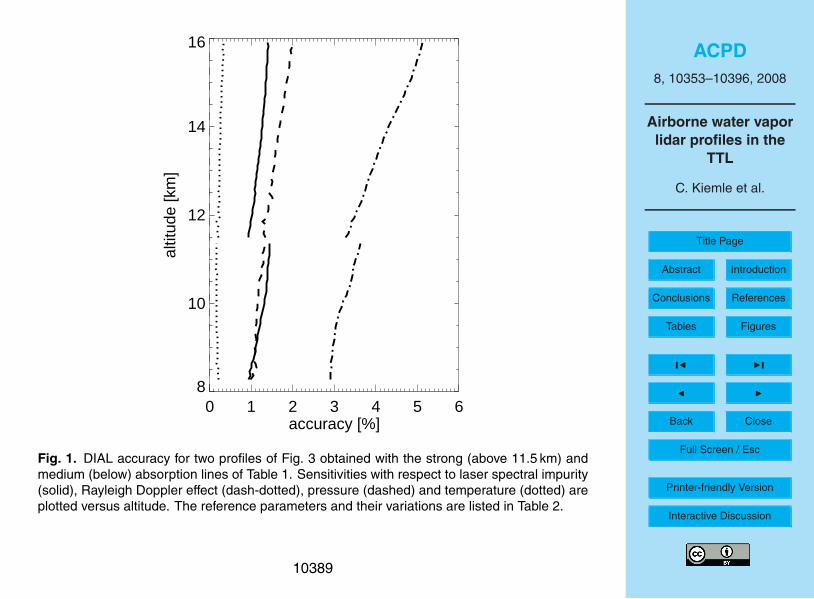
ACPD

8, 10353–10396, 2008



TTL

C. Kiemle et al.

Title Page



Tables Figures

◭ ◮

◭ ◮

Back Close

Full Screen / Esc



0 1 2 3 4 5 6accuracy [%]

8

10

12

14

16

altit

ude

[km

]

Fig. 1. DIAL accuracy for two profiles of Fig. 3 obtained with the strong (above 11.5 km) and

medium (below) absorption lines of Table 1. Sensitivities with respect to laser spectral impurity

(solid), Rayleigh Doppler effect (dash-dotted), pressure (dashed) and temperature (dotted) are

plotted versus altitude. The reference parameters and their variations are listed in Table 2.

10389





ACPD

8, 10353–10396, 2008



TTL

C. Kiemle et al.

Title Page



Tables Figures

◭ ◮

◭ ◮

Back Close

Full Screen / Esc



Fig. 2. Vertical cut of DIAL water vapor volume mixing ratio through the anvil outflow of a

deep convective system into the clear-sky TTL on 3 March 2004 at 13:06 UTC. The horizontal

resolution is 2 km, the vertical 100 m (300 m) at the bottom (top). The thunderstorm was located

∼100 km to the right.

10390





ACPD

8, 10353–10396, 2008



TTL

C. Kiemle et al.

Title Page



Tables Figures

◭ ◮

◭ ◮

Back Close

Full Screen / Esc



1 10 100 1000mixing ratio [µmol/mol]

4

6

8

10

12

14

16al

titud

e [k

m]

-40 -20 0 20 40mixing ratio difference [%]

4

6

8

10

12

14

16

altit

ude

[km

]

Fig. 3. Comparison between DIAL profiles (solid) and the TDLAS (tunable diode laser; red

dotted) hygrometer onboard the HIBISCUS SF1 balloon during its ascent on 16 February 2004

at 21 UTC. Water vapor volume mixing ratio (left) and relative differences (right) computed after

Eq. (1). Between 8 and 11 km altitude the horizontal water vapor variability (yellow box) is esti-

mated to ±20% from the DIAL data. Larger tropospheric variability below 8 km altitude and the

failure of the TDLAS above 11 km limit the useful comparison range. Note the excellent overlap

between individual subsequent DIAL profiles, confirming the high instrument’s accuracy.

10391





ACPD

8, 10353–10396, 2008



TTL

C. Kiemle et al.

Title Page



Tables Figures

◭ ◮

◭ ◮

Back Close

Full Screen / Esc



1 10 100mixing ratio [µmol/mol]

10

12

14

16

18

altit

ude

[km

]

-60 -40 -20 0 20 40 60mixing ratio difference [%]

10

12

14

16

18

altit

ude

[km

]

a

18.1.05


10

12

14

16

18

altit

ude

[km

]


10

12

14

16

18

altit

ude

[km

]

b

20.1.05


10

12

14

16

18

altit

ude

[km

]


10

12

14

16

18

altit

ude

[km

]

c

15.2.05


10

12

14

16

18

altit

ude

[km

]


10

12

14

16

18

altit

ude

[km

]

d

27.2.05


10

12

14

16

18

altit

ude

[km

]


10

12

14

16

18

altit

ude

[km

]

e

27.2.05

Fig. 4. Comparison between DIAL (black), FISH (blue) and FLASH (red) profiles from Geophysica descents. Left:Water vapor volume mixing ratio and ice saturation from Geophysica temperature measurements with ±1 K uncertaintyrange for DIAL profile altitudes (light blue). Right: differences between DIAL and FISH (FLASH) in blue (red) computedafter Eq. (1). Yellow boxes: water vapor variability estimated to ±5% (a), ±10% (b), ±8% (c), ±20% (d) and ±24% (e)from the DIAL.

10392





ACPD

8, 10353–10396, 2008



TTL

C. Kiemle et al.

Title Page



Tables Figures

◭ ◮

◭ ◮

Back Close

Full Screen / Esc




11

12

13

14

15

16

17

18

altit

ude

[km

]

Fig. 5. Overview of all relative differences from Fig. 4 between DIAL and FISH (FLASH) in

blue (red); overall averages solid. The average profiles have discontinuities at altitudes where

individual profiles stop. Above 15.5 (17.3) km altitude the average difference with FISH (FLASH)

is from Fig. 4a only. Positive difference means DIAL drier. There is no significant altitude-

dependent bias.

10393





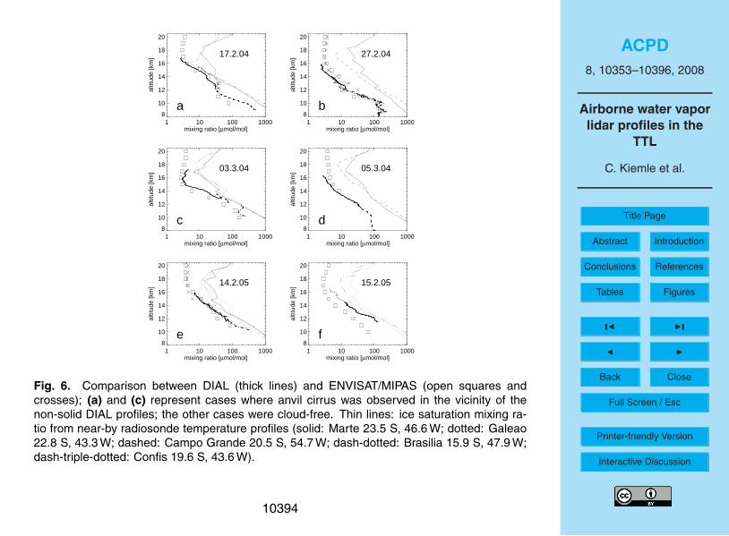
ACPD

8, 10353–10396, 2008



TTL

C. Kiemle et al.

Title Page



Tables Figures

◭ ◮

◭ ◮

Back Close

Full Screen / Esc




8

10

12

14

16

18

20

altit

ude

[km

]

a

17.2.04


8

10

12

14

16

18

20

altit

ude

[km

]

b

27.2.04


8

10

12

14

16

18

20al

titud

e [k

m]

c

03.3.04


8

10

12

14

16

18

20

altit

ude

[km

]

d

05.3.04


8

10

12

14

16

18

20

altit

ude

[km

]

e

14.2.05


8

10

12

14

16

18

20

altit

ude

[km

]

f

15.2.05

Fig. 6. Comparison between DIAL (thick lines) and ENVISAT/MIPAS (open squares and

crosses); (a) and (c) represent cases where anvil cirrus was observed in the vicinity of the

non-solid DIAL profiles; the other cases were cloud-free. Thin lines: ice saturation mixing ra-

tio from near-by radiosonde temperature profiles (solid: Marte 23.5 S, 46.6 W; dotted: Galeao

22.8 S, 43.3 W; dashed: Campo Grande 20.5 S, 54.7 W; dash-dotted: Brasilia 15.9 S, 47.9 W;

dash-triple-dotted: Confis 19.6 S, 43.6 W).

10394





ACPD

8, 10353–10396, 2008



TTL

C. Kiemle et al.

Title Page



Tables Figures

◭ ◮

◭ ◮

Back Close

Full Screen / Esc



-150 -100 -50 0 50 100mixing ratio difference [%]

10

12

14

16

altit

ude

[km

]

17.2.04

27.2.04

03.3.04

05.3.04

14.2.05

15.2.05

Fig. 7. Overview of relative differences between DIAL and ENVISAT/MIPAS from Fig. 6. The

overall mean (black line) and standard deviation is –8.3%±48.5%, above 12 km –3.2%±48.8%.

Negative difference means DIAL more humid.

10395





ACPD

8, 10353–10396, 2008



TTL

C. Kiemle et al.

Title Page



Tables Figures

◭ ◮

◭ ◮

Back Close

Full Screen / Esc



1 10 100 1000 10000mixing ratio [µmol/mol]

4

6

8

10

12

14

16

18

altit

ude

[km

]

48 N 18.1.0540 N 20.1.0535 N 27.2.0515 N 27.2.05

18 S 17.2.0418 S 03.3.0418 S 14.2.0520 S 15.2.0522 S 16.2.0422 S 27.2.0422 S 03.3.0422 S 05.3.04

Fig. 8. Overview of all 35 DIAL water vapor profiles used in the study (thick lines). Thin lines: ice

saturation mixing ratio from near-by radiosonde temperatures. Tropical standard atmosphere

mixing ratio (ice saturation) as thin solid (dashed) black line for comparison. Within 11 and

16 km a relatively smooth exponential transition from tropospheric to stratospheric humidity is

observed. The hygropause with a minimum mixing ratio of ∼2.5µmol/mol is located between

15 and 16 km altitude, the cold point tropopause from the radiosonde temperatures at around

17 km.

10396





first airborne water vapor lidar measurements in the

Documents