first principles description of response functions in low...
TRANSCRIPT

First principles description of response
functions in low dimensional systems
Doctoral thesis submitted by
Daniele Varsano
for the degree of
Doctor of Physics
March 2006


Contents
Preliminaries v
I Basic concepts 1
1 Basic foundation of DFT 71.1 Approximation to the Exchange and Correlation Functionals . . . . . 101.2 Some problems and pathologies of present xc functionals . . . . . . . 13
1.2.1 The Band Gap problem . . . . . . . . . . . . . . . . . . . . . 131.2.2 The xc Electric Field . . . . . . . . . . . . . . . . . . . . . . . 14
2 Time-dependent DFT (TDDFT) 172.1 Basic theorems . . . . . . . . . . . . . . . . . . . . . . . . . . . . . . 172.2 Excitation energies in TDDFT . . . . . . . . . . . . . . . . . . . . . . 19
2.2.1 Matrix eigenvalue method . . . . . . . . . . . . . . . . . . . . 212.2.2 Full solution in real time of the TDDFT Kohn-Sham equations 24
2.3 Dielectric Function . . . . . . . . . . . . . . . . . . . . . . . . . . . . 25
3 Many Body Perturbation Theory 293.1 Quasiparticle formulation . . . . . . . . . . . . . . . . . . . . . . . . . 293.2 Hedin’s Equations . . . . . . . . . . . . . . . . . . . . . . . . . . . . . 343.3 The GW approximation . . . . . . . . . . . . . . . . . . . . . . . . . 353.4 Two particle effects . . . . . . . . . . . . . . . . . . . . . . . . . . . . 373.5 Combining MBPT and TDDFT . . . . . . . . . . . . . . . . . . . . . 43
II Numerical and technical developments 47
4 Numerical implementations 494.1 Real Space - Real Time representation: the OCTOPUS project . . . . . 51
4.1.1 The Grid . . . . . . . . . . . . . . . . . . . . . . . . . . . . . 514.1.2 The Time Evolution . . . . . . . . . . . . . . . . . . . . . . . 52
4.2 Plane waves . . . . . . . . . . . . . . . . . . . . . . . . . . . . . . . . 534.3 Technical details and implementations in the code SELF . . . . . . . . 55
5 An exact Coulomb cutoff technique for supercell calculations 615.1 The 3D-periodic case . . . . . . . . . . . . . . . . . . . . . . . . . . . 635.2 System with reduced periodicity . . . . . . . . . . . . . . . . . . . . . 645.3 Cancellation of singularities . . . . . . . . . . . . . . . . . . . . . . . 69

iv
5.4 Results . . . . . . . . . . . . . . . . . . . . . . . . . . . . . . . . . . . 735.4.1 Ground state calculations . . . . . . . . . . . . . . . . . . . . 745.4.2 Static polarizability . . . . . . . . . . . . . . . . . . . . . . . . 765.4.3 Quasiparticles in the GW approximation . . . . . . . . . . . . 805.4.4 Exciton binding energy: Bethe-Salpeter equation . . . . . . . 825.4.5 Comparison between real-space and plane wave codes . . . . . 85
III Applications 89
6 Optical spectroscopy of biological chromophores 916.1 Excited states of DNA bases and their assemblies . . . . . . . . . . . 92
6.1.1 Computational Framework . . . . . . . . . . . . . . . . . . . . 956.1.2 Isolated gas-phase nucleobases . . . . . . . . . . . . . . . . . . 986.1.3 Watson-Crick pairs GCH and ATH . . . . . . . . . . . . . . . . 1086.1.4 Stacked GCs and d(GC) structures . . . . . . . . . . . . . . . 112
6.2 The Green Fluorescent Protein . . . . . . . . . . . . . . . . . . . . . 1186.2.1 Computational Framework . . . . . . . . . . . . . . . . . . . . 1206.2.2 Results . . . . . . . . . . . . . . . . . . . . . . . . . . . . . . . 123
7 Optical absorption of quasi 1D systems 1297.1 Description of the systems . . . . . . . . . . . . . . . . . . . . . . . . 1327.2 One Monomer spectra . . . . . . . . . . . . . . . . . . . . . . . . . . 1337.3 Optical properties of finite chains . . . . . . . . . . . . . . . . . . . . 1367.4 Infinite chains . . . . . . . . . . . . . . . . . . . . . . . . . . . . . . . 146
7.4.1 Trans-Polyacetylene . . . . . . . . . . . . . . . . . . . . . . . . 1467.4.2 Hydrogen chain . . . . . . . . . . . . . . . . . . . . . . . . . . 150
7.5 Conclusion . . . . . . . . . . . . . . . . . . . . . . . . . . . . . . . . . 157
8 Photo-electron spectroscopy in TDDFT framework 1598.1 One-electron spectroscopy . . . . . . . . . . . . . . . . . . . . . . . . 161
8.1.1 Mask-function approach . . . . . . . . . . . . . . . . . . . . . 1638.2 Many-body photo-electron spectroscopy . . . . . . . . . . . . . . . . . 165
8.2.1 Density-matrix approach . . . . . . . . . . . . . . . . . . . . . 1668.2.2 Population analysis . . . . . . . . . . . . . . . . . . . . . . . . 168
8.3 Results . . . . . . . . . . . . . . . . . . . . . . . . . . . . . . . . . . . 171
9 Two photon-photoemission spectra of Cu metal surfaces 1799.1 Introduction . . . . . . . . . . . . . . . . . . . . . . . . . . . . . . . . 1799.2 Description of the model for CU(100) and CU(111) surfaces . . . . . 1829.3 Energy-resolved spectra . . . . . . . . . . . . . . . . . . . . . . . . . 1869.4 Time-resolved spectra . . . . . . . . . . . . . . . . . . . . . . . . . . . 188
A Publications 191
Acknowledgments 193
Preliminaries
In the last decades a big effort in both technological and fundamental research has
been devoted to what is generically called “nanotechnology”. Even if this is a generic
term it can be defined as the understanding and control of matter at the nanometer
scale, i.e. the scale of single atoms and small molecules and biology. This has
important implications to many fields of research from chemistry to materials science
passing by biophysics. In this regime classical physics is not valid anymore and the
principles of quantum mechanics have to be applied. Unique phenomena occurring
at this scale could enable novel applications [Nalwa 05]. Insight into the nature of
microscopic matter has been possible thanks to an increasing and rapid development
of optical, electronic and time-resolved spectroscopic techniques that allow more and
more precise and detailed measurements and control of the ”nanoworld”. In step
with such progress in the field of experimental physics, there has been a big effort
by the scientific community to achieve a more detailed theoretical description of the
properties of materials at the nanoscale.
Thanks to the recent theoretical developments and the increases in computa-
tional power, numerical calculations of real systems have also been made possible.
In particular, ab-initio methods are nowadays indispensable for a through under-
standing of properties and phenomena in low-dimensional structures. Among these,
Density Functional Theory (DFT) occupies a dominant place. By replacing the
interacting many-electron problem with an effective single-particle problem, DFT
allows the density to be computed faster, so it can be used to calculate ground
state properties of large systems: remarkable results have been achieved for ground
state properties of a huge number of systems ranging from atoms and molecules
to solids and surfaces. However, insight into the microscopic nature of matter can
only be gained through the interaction of external probes with matter, i.e, through
the understanding of excitations (as probed by infrared, Raman, electron and op-
tical spectroscopies for instance) and hence the theoretical prediction of response
properties is of fundamental interest. The development of ab-initio techniques that
are capable of predicting excited-state quantities, as reliably as, DFT does for the
ground state, is a real challenge. In recent years Time Dependent Density Func-
tional Theory (TDDFT) has emerged as a valuable tool for extracting electronic
v

vi
excited state energies by applying the same philosophy of DFT to time-dependent
problems. Its basic variable is the one body density that is obtained from the so-
lution of a fictitious system of non-interacting electrons that evolves in an effective
potential vs(r, t) containing all the many-body effects in its exchange and correlation
part. As in the ground state case, it has the big advantage of computational speed
with respect to other methods that rely on wave-functions and on the many-body
Schrodinger equation. TDDFT can be viewed as an exact alternative reformulation
of time-dependent quantum mechanics, nevertheless it has its own drawbacks and
cannot be applied with success in all situations. The failures of the theory have
to be attributed to the needed approximation of the unknown effective potential
vs(r, t). In any case TDDFT offers a suitable compromise between accuracy and
computational efficiency, permitting the description of quite large systems (∼ 500
atoms). This feature makes the TDDFT as a suitable tool for the study of so-
phisticated systems, including phenomena of biological interest. One of the goal
of modern biology is the understanding of biological phenomena at the molecular
level, which involves the study of the structure of biomolecules and their functions,
as well as excited states and interaction between the biomolecules and the electro-
magnetic field. Biological systems are particularly challenging for ab-initio quantum
mechanical methods, nevertheless first principles calculations can be used to attack
problems of great current biological interest, that cannot be solved by different ap-
proach, and can provide results for comparison with a variety of spectroscopic data.
The application of ab-initio techniques for these classes of complex systems was
considered as “utopian” until a few years ago, due to the extremely high degree of
complexity. Moreover the TDDFT is perfectly general and can be applied to any
time-dependent problem, including the non-perturbative regime, and the description
of non linear-phenomena.
The challenge of describing nano and bio structures of potential technological
applications imply developments of two sorts: firstly, the proper treatments of many-
body effects in simplified, although in principle exact theories (density functional
based), secondly the the development of new algorithms and technique, as numerical
implementations to speed up the calculations. The present work address both topics,
within TDDFT, to describe the response properties of low dimensional structures
to external perturbations, in particular the optical properties of low dimensional
systems, including biomolecules. The latter would be the focus of a large part of
the research done in this thesis. Armed with this theoretical tool we have studied
two biological systems of great relevance. First of all we have investigated the

vii
optical properties of DNA bases and base pairs, analyzing in detail the impact of
the hydrogen bonding and π stacking in the absorption spectra for both Watson-
Crick base pairs and Watson-Crick stacked assemblies. Insight into the excited states
of DNA turns to be important not only for understanding crucial phenomena such
as radiation-induced DNA damage, but also because of the growing interest in this
molecule for various applications in nanotechnology. Secondly, we have successfully
employed the method for the description of the linear response of the chromophore of
the Green Fluorescent Protein, a molecule whose characteristics of fluorescence and
inertness are extensively used in molecular biology as a marker of gene expression.
Of course the specific exchange correlation approximations used in TDDFT, like all
physical theories, does not work for all systems and situations. For instance, it is
known to fail in the description of optical properties of long, conjugated molecular
chains A similar problem is encountered in the calculation of excitations of non-
metallic solids when treated with standard functionals As mentioned before, the
origin of this failure has to be attributed to the choice of the exchange and correlation
part of the effective potential, and the problem is related to a non local dependence
of the xc potential. In order to get insight in this problematic we have studied
this class of systems (conjugated linear molecular chains) firstly using Many Body
Perturbation Theory (MBPT) and secondly within TDDFT framework, using a
new non-local and energy-dependent exchange and correlation potential extracted
from the MBPT. Absorption spectra in MBPT has been calculated by means of the
Bethe-Salpeter (BS) equation. The BS equation takes into account the electron-hole
interaction, which cannot be omitted from a description of neutral excitations (e.g.
optical and energy loss spectra), especially for semiconductors and insulators. In
the last few years the BS equation has be proved to give remarkably good results
for the absorption of a large variety of systems: insulators, semiconductors, atoms,
clusters, surfaces and polymers. The absorption spectra calculated by BS equation
have been then compared with TDDFT calculations. The obtained results obtained
with new functional turn to be of the same precision as the BS, removing the huge
error committed by local and gradient-corrected functionals. A lot of work has
been done in the last years in order to marry MBPT and TDDFT, this studies
have been successful and provide a consistent scheme to include many body effects
into TDDFT for solids. The question of validity of this scheme for low dimensional
structures, including polymers, nanotubes, biomolecules and nanostructures is still
under debate. This thesis shows how all those systems can described on the same
footing, providing a consistent theoretical framework to deal with the interaction of
viii
matter with external probe. Of course this is not the final answer as correlations have
been introduced at a very simplified level, the next quest would be to add correlation
at higher orders that are, of course, relevant for many materials. We hope the present
thesis contributes a step forward to achieve this goal. The studied systems are trans-
polyacetylene and a molecular hydrogen chain. Trans-polyacetylene is a very well
studied conjugated polymer, and is used in a wide range of applications, such as
light emitting diodes, photo-diodes and photo-voltaic cells. The molecular hydrogen
chain is a model system that can be used to explain different features of real systems
by varying the bond length alternation of the chain.
Finally, in the last part of this work, we have studied systems in intense laser
fields with electric field strengths that are comparable to the attractive Coulomb field
of the nuclei. In this situation the time-dependent field cannot be treated perturba-
tively; while to solve the time-dependent Schrodinger equation for the evolution of
two interacting electrons is barely tractable with present-day computer technology.
For such systems TDDFT offers a practical alternative and is able to describe non-
linear phenomena like high-harmonic generation, or multi-photon ionization. In this
context we have developed a feasible computational procedure to calculate, within
TDDFT, the photo-electron spectrum (PES) of atoms and clusters when excited by
short laser pulses. The computational procedure relies on a geometrical approach
and provides a description of both energy and angle resolved photo-electron spectra.
In order to validate the method we have applied this scheme to a 1D two-electron sys-
tem and described a energy-resolved and time-resolved two-photon photo-emission
experiment on copper surfaces using a 1D model potential.
This dissertation is divided into three parts, and is organized as follows. In the
first part, we describe the basic concepts and theories used. In chapter (1) we out-
line the basic foundation of DFT, while chapter (2) is dedicated to the extension
of the theory to time dependent problems (TDDFT) with a particular attention in
describing the methods that enable the calculation of excited states. In chapter (3)
we give a short introduction to the key concepts of Many Body Perturbation The-
ory, and the last part of this chapter is focused on the combination of TDDFT and
MBPT to describe the new kernel to be used later in chapter (7). The second part of
the thesis aims to provide the numerical details and the practical implementations
of the theories described in the first part, (this is described in chapter (4)), while in
chapter (5) we illustrate a newly developed Coulomb cutoff technique that permits
to treat systems that are periodic in less than three dimensions with supercell tech-

ix
niques. This method has been extensively used in the work discussed in chapter (7).
The third part of the thesis collects the results of the studied systems: chapter (6)
is dedicated to the optical spectroscopy of biological chromophores: the DNA bases
and base pairs and the chromophore of the Green Fluorescent Protein. The optical
absorption of linear chains and infinite polymers studied with MBPT and TDDFT
with the new kernel is discussed in chapter (7). Chapter (8) and (9) are devoted to
photo-electron spectroscopy: in chapter (8) we describe our new approach to obtain
the photo-electron spectrum within TDDFT, based on geometrical considerations
and we apply such method to a model two-electron 1D atom, while in chapter (9) we
apply the same scheme to obtain energy- and time- resolved photoemission spectra
of image states in Cu(100) and Cu(111) surfaces.

x

Part I
Basic concepts
1

3
The great step made forward by Density Functional Theory (DFT) is to furnish
a theoretical basis to a general problem of the Quantum Mechanics: by substituting
the many body wave function of an electron system Ψ(r1, ..., rN) (defined in a 3N
dimensional space) with the electron density of the system (a three dimensional
function) as basic variable:
n(r) = N
∫
dr2..drN |Ψ(r, r2, ..rN)|2 (1)
One of the earliest attempt to solve a many body electron problem is due to Hartree
[Hartree 28], who approximated the wave function Ψ as a product of single particle
wave functions ψ(ri). Each single particle orbital satisfies a one-electron Schrodinger
equation with a local potential arising from the average field of all other electrons.
Clearly Hartree’s solution ignores Fermi statistics and produces a fully uncorrelated
solution. Slater and Fock [Slater 30, Fock 30] included fermion statistics, writing
the wave function Ψ as a single Slater determinant, which leads to the Hartree Fock
approximation with a non-local exchange term in the single particle Schrodinger
equation. In such approximation electrons of the same spin are correlated, but cor-
relation between electron of different spin is totally neglected. Along this direction,
where the many body wave function is the basic variable, there exists a number of
methods of increasing complexity. An example of them is the configuration inter-
action method (CI) where the ground state wave function is a linear combination
of a given number of Slater determinant that minimizes the energy. This method
leads in principle to the exact many-particle wave-function, but the number of nec-
essary configurations increases drastically with the number of electrons, and the
application of such method to large system is prohibitive. A completely different
approach was taken by Thomas and Fermi [Thomas 27, Fermi 28], who earlier on
proposed a scheme based on the density of the electron system. They assumed that
the motions of the electrons are uncorrelated, and that the kinetic energy of a sys-
tem of density n can be described with a local functional of the density obtained
from the kinetic energy of free electrons. Although the Thomas Fermi approxima-
tion has only limited success in treating real materials, it is the basis of the density
functional formalism. Sharp and Horton [Sharp 53] look to the best local potential
that reproduces the non-local Hartree-Fock scheme. This OEP (Optimized Effec-
tive Potential) scheme is nowadays widely used in the DFT community to handle
orbital-dependent functional, that we will briefly describe later, and it can be con-
sidered a firsts step toward the concept of Kohn-Sham orbitals in DFT developed
later on in 1965. However, the theoretical foundation that permits this substitu-

4
tion was established only in the 1964, by Hohenberg and Kohn [Hohenberg 64] who
demonstrated that the ground state density of a non degenerate system of interacting
electrons determines implicitly all the properties derivable from the Hamiltonian of
the system. 1 This is the theoretical basis of the Density Functional Theory (DFT).
In a following paper [Kohn 65] Kohn and Sham furnished a practical scheme based
on the Hohenberg and Kohn (HK) theorem that permits to solve the many body
equation through an auxiliary fictitious non-interacting system that obeys a set of
single particle equations, the so-called Kohn-Sham equations (KS).
Currently the DFT and in particular the KS scheme is the most widely used
method in electronic structure calculation in the condensed matter physics com-
munity. In this chapter we will briefly remind the theoretical foundation of the
(DFT) and its time dependent extension: the Time Dependent Density Functional
Theory (TDDFT) which are the methods used in most all the works exposed in
this thesis. We will not enter here in the mathematical details of the theories, but
we will limit to expose the basic principles and explain the main equations that
have been extensively used in this thesis, and we refer the reader to the following
reviews and books for further details and deeper discussion. For the DFT we re-
fer to Refs [Dreizler 90, Kohn 99, Lundqvist 83, Seminario 96], and for TDDFT to
Refs:[Gross 96, Fiolhais 03, Marques 04, Jamorsky 96, van Leeuwen 01, Burke 02].
A recent summary of the TDDFT theory with applications and discussion of all limi-
tations and benefits can be found in[Marques 06]. In the first two chapters we will re-
vise the fundamental theorems that constitutes respectively the basis of the DFT and
TDDFT describing also the main approximations used in the practical applications,
and in the third section we will describe different schemes that we have employed to
calculate excitations energies in TDDFT. With respect the DFT we will follow the
derivation of Levy [Levy 79] that it is more general than the original derivation of
Hohenberg and Kohn and includes also degenerate ground states. In this chapter we
ignore the spin of the electrons, except for considering their fermionic character, and
the basic variable will be the spin-less density. For an extension of the theory to the
spin-dependent case (useful when treating spin-dependent external-potential or rel-
ativistic corrections) we refer to Ref.[Fiolhais 03, von Barth 72]. There exists other
extension of the theory as the multicomponent DFT [Kreibich 01] developed to treat
both electrons and nuclei quantum mechanically on the same footing and the DFT
for superconductors to [Luders 05, Marques 05]. Note that also there exists func-
1 The Nobel Prize in Chemistry 1998 was awarded to Walter Kohn for his development of the
Density Functional Theory.

5
tional theories based on the current as basic variable (Current DFT). Those are not
treated in the present work, therefore we refer the reader to [Vignale 87, Vignale 88]
for details. We use atomic units (e2 = ~ = m = 1) unless otherwise stated.

6

1 Basic foundation of DFT
Let us consider a set of systems of N electrons subject to an external potential ν(r).
The Hamiltonian is:
H(r1, r2, ..., rN) =
N∑
i=1
(
− 1
2∇2
ri+ ν(ri)
)
+1
2
N∑
i6=jv(ri, rj) (1.1)
The Hamiltonian can be cast in the form: H = T + Vee+ Vext, where T is the kinetic
energy operator,Vee is the electron-electron interaction and Vext =∑
i ν(i) is the
external potential. We start by defining the set of N-representable densities NN .
This is the set of the densities n(r) that can be obtained from some antisymmetric
wave function of N electrons. Next we define the set of ν-representable densities Nν:
the set of densities n(r) which are ground-state of any N electron system for some
external potential ν. Now we define the Levy-Lieb functional F [Levy 79] as:
F [n] = minΨ→n
〈Ψ|T + Vee|Ψ〉, n ∈ NN (1.2)
here the minimum is taken over all the antisymmetric N-electrons wave function
that yield the interacting density n. The functional F is universal and well defined
[Lieb 82]. Let’s denote by Ψmin[n] the wave-function that minimizes the functional
for the interacting system for a given density. Now we define a new energy functional
with respect to the external potential:
Eν[n] = F [n] + Eext[n] = F [n] +
∫
drn(r)ν(r) (1.3)
where Eν[n] is the expectation value of the Hamiltonian evaluated with the state
Ψmin[n]:
Eν[n] = 〈Ψmin[n]|H|Ψmin[n]〉 (1.4)
This implies by construction that the energy functional Eν [n] is an upper bound for
the ground state energy, and present a global minimum at exactly the ground state
density.:
Eν[n] ≥ EGS, ∀n ∈ Nν (1.5a)
Eν [nGS] = EGS (1.5b)
7

8 Chapter 1. Basic foundation of DFT
To obtain the ground state density we need to minimize Eν [n] with respect to
the density imposing the normalization constrain∫
drn(r) = N with a Lagrange
multiplier µ:∂F
∂n(r)+ ν(r) = µ (1.6)
where µ coincides with the chemical potential. If we rewrite the expression (1.6) for
the ground state density:
ν(r) = µ− ∂F
∂n(r)[nGS] (1.7)
we learn that the external potential is univocally determined by the ground state
density. So if we know the external potential, we know the full Hamiltonian, and
this implies in principle the knowledge of all the properties of the system. From
those statements we can conclude that the ground state density is enough to extract,
in principle, all physical quantities of a fermionic system.
Anyway this does not provide any practical scheme to obtain the ground state
density nGS. To achieve this purpose Kohn and Sham introduce an auxiliary system
of non-interacting electrons having the same density as the interacting one. We
denote this system with the letter S. This system is subject to an external potential
νS. The functional F[n] for this fictitious system reduces to:
FS[n] = TS[n] = minΨ→n
〈Ψ|T |Ψ〉, n ∈ NN (1.8)
In analogy to Eq. (1.6) for the non-interacting system S we have:
∂TS∂n(r)
+ νS(r) = µ (1.9)
By comparing Eq(1.6) and Eq(1.9) we get a formal expression for νS[n]:
νS[n] = ν(r) +∂F
∂n(r)− ∂TS∂n(r)
(1.10)
This implies that the solution of the non-interacting system is the same of the in-
teracting one. In this way we get the interacting density, because we know how to
calculate the ground state density of a non-interacting system via its representa-
tion in Slater determinant (Kohn-Sham orbitals) and the solutions of the associated
single particle equations (Kohn-Sham Equations). In order to make explicit these
equations we start by defining the exchange-correlation energy and its functional
derivative (the xc potential vxc) as:
Exc[n] =F [n] − TS[n] − U [n] (1.11)
vxc[n](r) =∂Exc∂n(r)
(1.12)
9
Here U[n] indicates the classical Hartree electrostatic energy functional:
U [n] =1
2
∫
drn(r)u[n](r), (1.13)
and its functional derivative provides the Hartree potential vH(r)
vH [n](r) =δU
δn(r)=
∫
dr′n(r′)
|r − r′| . (1.14)
Then now we have a close expression for the effective potential νS[n] of the non-
interacting system:
νS[n](r) = ν(r) + vH [n](r) + vxc[n](r) (1.15)
This potential is called Kohn-Sham potential vKS.The corresponding Kohn-Sham
Hamiltonian will be hKS = t + vKS[n], where t is the one-particle kinetic operator
[−∇2
2]. In summary the ground state density of the system can be calculated solving
self consistently the following set of Kohn-Sham equations:
hKS[n]|ψj〉 =εj|ψj〉 (1.16a)
hKS[n] = −1
2∇2 + ν(r) +
∫
dr′n(r′)
|r − r′| + vxc[n](r) (1.16b)
n(r) =∑
j
θ(µ− εj)ψ∗j (r)ψj(r) (1.16c)
∫
drn(r) = N (1.16d)
where ψj, are the one particle wave function that are solution of the non-interacting
problem Eq. (1.16a). The Fermi level µ of Eq. (1.9) is determined by the fulfillment
of Eq. (1.16d). Thus, the ground state total energy EGS of the interacting system
is given by:
EGS =∑
j
θ(µ− εj)εj − U [n] −∫
drn(r)vxc[n](r) + Exc[n] (1.17)
In principle the solution of the Kohn-Sham equation with the exact exchange-
correlation potential, would give single particle eigenstates which density equals
the exact density of the interacting system. Clearly the exact xc-potential, which
includes all non-trivial many body effects, it is unknown and has to be approximated.
The Exc[n] term, even if it is a small part of the total energy for typical chemical
system, it is of the order of magnitude of the atomization energy, the relevant mag-
nitude in Chemistry, so good approximations are required. We will show later how
Many-body perturbation theory can be used to improve available xc-functionals for
electronic properties.
10 Chapter 1. Basic foundation of DFT
1.1 Approximation to the Exchange and Correla-
tion Functionals
The research on the optimal exchange-correlation potential has been a flourishing
field of research in the last decades, and very good xc-functionals are now available1.
One of the most widely used and simplest approximation, is the Local Density
Approximation (LDA). In this thesis this has been the most used approximation for
our ground state calculation. However when needed we compare with more precise
schemes as GGA’s. Introducing the exchange-correlation energy density εxc([n]; r),
we can write the xc Energy as:
Exc[n] =
∫
drn(r)εxc([n]; r). (1.18)
the LDA assumes that the system locally appears as an homogeneous electron gas
of the same density as the inhomogeneous system:
ELDAxc [n] =
∫
drn(r)εHEGxc (n)(r) (1.19)
εHEGxc ([n]; r) is split in its bare exchange part and correlation part. While the ex-
change part is an analytic function of n [Fetter 81].
εHEGx (n(r)) = −3
4
[3n
π
]1/3
(1.20)
the correlation part can be approximated using Many Body perturbation theory
[Hedin 71], or obtained from Quantum Montecarlo methods [Ceperley 80]. The
results from Quantum Montecarlo calculation has been parametrized by, e.g. Perdew
and Zunger [Perdew 81] and also allow the treatment of spin polarized system (local
spin density approximation LSD). In this thesis, however, we have considered only
the case if spin compensated systems. The correlation part is given by:
εHEGc (n(r)) = γ/(1 + β1
√
(rs) + β2rs), rs ≥ 1 (1.21)
where rs is defined by:1
n(r)=
4
3πr3
s (1.22)
and γ = −0.14230, β1 = 1.05290 , β2 = 0.3334. The LDA approximation should
be a good approximation for systems with slow varying density. Anyway LDA has
1 For example see: J. P.Perdew and S. Kurth in Chap.1 of [Fiolhais 03]
1.1 Approximation to the Exchange and Correlation Functionals 11
been applied successfully for a big amount of systems , and its success rely to error
cancellations [Dreizler 90, Jones 89], and from the fact that important sum rules are
exactly satisfied in LDA. Nevertheless we have to mention several shortcomings of
the LDA among that:
• The LDA does not work for system where the density has strong spatial vari-
ations or for weakly interacting system as Van der Waals bonded molecules.
It usually overestimates correlation and underestimates exchange.
• The exchange part of the functional does not cancel the self-energy part of the
Hartree term with the consequence of a wrong asymptotic behavior of the xc
potential for finite systems. Such shortcomings leads to wrong estimation of
ionization potentials of atoms and molecules, Rydberg states are not present
in LDA and negative ions usually does not bind
Another class of functionals that we also used in this thesis is the so-called General-
ized Gradient Approximated (GGA) functionals [Becke 88, Lee 88, Perdew 96]. For
these functionals the exchange-correlation energy is written as:
EGGAxc [n] =
∫
drn(r)εGGAxc (n(r),∇n(r)) (1.23)
εGGAxc is some analytic function of the density and the gradient of the density with
some free parameters, that are either fitted to experiments or obtained from sum
rules. The GGA functionals solve some of the problems present in LDA, in gen-
eral atomic and molecular total energies are improved, and are extensively used in
quantum chemistry calculations. Recently another family of functionals has been
introduced that generalize the GGA approximation, called Meta-GGA functionals
[Perdew 99], where εMGGAxc is now a functional not only of the density and its gra-
dient , but also of the kinetic energy density 2. Such extra-dependence permits to
have more flexibility and more precise approximations to the exact xc functional
have been obtained. Anyway neither the GGA nor the MGGA approximations
solve the self-interaction problem. We finish this section mentioning another class
of xc-potential that we have also used in this thesis, the so-called Optimize Effective
Potential (OEP)3. This family of potential is formed by functionals that have an
explicitly dependence on the Kohn-Sham orbitals thus are only implicitly functional
2 Due to the dependence on the kinetic energy density, the MGGA, are orbital functionals.3 For a review on this generation of functional see i.e.: E.Engel in Chap.2 of [Fiolhais 03]

12 Chapter 1. Basic foundation of DFT
of the density. Thus, the OEP scheme looks for the local potential that minimize
the energy functional with respect to the density.
EOEPxc = EOEP
xc [ψ1(r)...ψN(r)] (1.24)
The xc potential is then calculated via Eq. (1.12) using the chain rules for functional
derivatives:
vOEPxc [n](r) =δEOEP
xc
δn(r)=
N∑
i=1
∫
dr′dr′′[δEOEP
xc
δψi(r′)
δψi(r′)
δvks(r′′)+ c.c
]δvks(r′′)
δn(r)(1.25)
Here the term δEOEPxc
δψi(r′)is obtained from the expression of EOEP
xc [ψ1(r)...ψN(r)], the
second derivatives δψi(r′)δvks(r′′)
can be calculated using first order perturbation theory
and finally δvks(r′′)δn(r)
is the inverse of the Kohn-Sham response function as we will see
in section (2.2). Equation (1.25) can be recast in an integral equation for vOEPxc . An
example of these orbitals functionals is the exact exchange (EXX) potential that is
derived applying the OEP-scheme to the exact expression for the exchange energy:
EEXXx = −1
2
∑
σ
N∑
i,j=1
∫
drdr′ψ∗jσ(r)ψ
∗iσ(r
′)ψiσ(r)ψjσ(r′)
|r− r′| (1.26)
Note that the EEXXx functional cancels the self-interaction part of the Hartree energy
and the exact exchange potential has the correct asymptotic behavior. Anyway,
the solution of the equations to get such xc potentials turns to be numerically
demanding, and approximations has been proposed to simplify the problem. In the
present work, (see section (7.4)), we have considered KS wave functions and energies,
by solving the OEP equation for the EEXXx within the Krieg-Li-Iafrate[Krieger 92]
(KLI) approximation:
vKLIx =1
2n(r)
∑
j
[
ψ∗j (r)
δEEXXx
δψ∗j (r)
+ c.c]
+ |ψj(r)|2∆vKLIj
(1.27a)
∆vKLIj =
∫
dr
θ(εj − µ)|ψj(r)|2vKLIx (r) − ψ∗j (r)
δEEXXx
δψ∗j (r)
+ c.c (1.27b)
The vKLIx then can be solved both by transforming the integral equations (1.27) in a
set of linear equations [Krieger 90] or one can iterate Eq. (1.27) until self-consistency.
It turn out that for most of the system studied the KLI approximation is very close
to the exact OEP solution [Fiolhais 03].
1.2 Some problems and pathologies of present xc functionals 13
1.2 Some problems and pathologies of present xc
functionals
1.2.1 The Band Gap problem
Before concluding this short description of the main feature of the DFT it is impor-
tant to emphasize that the KS eigenvalues obtained from Eq. 1.16a does not have
a physical meaning, except the highest occupied eigenvalues ε(N)N
4 which equals the
ionization potential of the system [Levy 84, Almbladh 85]. Even if the relative values
of the occupied KS eigenvalues are in rather good agreement with the experiment for
semiconductor and insulators, the band gaps are underestimated by about 50% up to
100%[Hybertsen 85, Hybertsen 86, Godby 86, Godby 87a, Godby 87b, Godby 88].
The exact band gap for an N electron system is defined by:
Egap = E(N+1) − E(N) −(
E(N) − E(N−1))
= ε(N+1)N+1 − ε
(N)N (1.28)
i.e the difference between the electron affinity and the ionization potential. For the
fictitious Kohn-Sham system we have:
EKSgap = ε
(N)N+1 − ε
(N)N (1.29)
From Eq. (1.28) and Eq. (1.29) we have:
Egap = EKSgap + ∆xc (1.30)
We may see that the quantity ∆xc is the difference between the energies of the (N+1)-
th orbitals of the KS systems that correspond to the neutral and ionized electron
system. The addition of an extra electron only induces an infinitesimal change of
the density, so a discontinuity of order one have to be assigned to a discontinuity in
the xc-potential, which is not necessarily analytic in N, in contrast to the Hartree
potential:
∆xc = V (N+1)xc (r) − V (N)
xc (r) (1.31)
There is evidence [Godby 88] that the xc discontinuity ∆xc, rather than the local
density approximation, is the main cause of the big discrepancy between the ex-
perimental values and the one found in DFT-LDA for typical semiconductors and
insulators. Thus we can say that the band gap problem is not an intrinsic feature
4 Here with ε(N)N we indicate the N-th eigenvalue of an (N)-electron system.

14 Chapter 1. Basic foundation of DFT
of the DFT nor of the LDA but of the Kohn-Sham scheme. In section (3.3) we will
see how realistic energies of adding/removing electron to/from the system can be
calculated within the quasiparticle formalism.
1.2.2 The xc Electric Field
Another important pathology of the exchange correlation potential vxc(r) is the so-
called exchange-correlation electric field [Godby 90, Godby 94, Gonze 95, Gonze 97a,
Gonze 97b, Ghosez 97]. If we consider an insulating solid subjected to an external
uniform electric field, the electrons in response of the electric field will generates
in each unit cell en electric dipole moment. The effect of the response of the elec-
tron will be a macroscopic polarization, and consequently a depolarizing electric
field that counteracts the external potential. If now we switch to the Kohn-Sham
system, Gonze et al. [Gonze 95] showed that the applied perturbing potential it is
not a unique functional of the periodic density, but it depends also on the change
in the macroscopic polarization, that is, on the electronic density at the surface of
the crystal. Moreover, the dependence of the exchange-correlation energy on po-
larization induces an exchange-correlation electric field. This situation is drawn in
Fig.(1.1). In the upper part is sketched the density charge and the KS potential of
an unpolarized insulator. When the electric field is applied (central and bottom part
of the figure) , the insulator is polarized and we see in the figure that two different
Kohn-Sham potential, one with zero net long range behavior (bottom part) and one
with a part that vary linearly in space (central panel), that reproduce the same bulk
density. The two potentials correspond to two different values of the macroscopic
polarizabilities. In particular it exists a family of potentials with different net long
range part, that gives the same bulk density and produce a different macroscopic
polarization. In order to reproduce the correct macroscopic polarization the ex-
change correlation potentials must have a particular non zero long range part. This
part of the exchange correlation potential it is the exchange-correlation electric field.
Therefore it is clear that the vxc(r) cannot be a functional of the density alone in the
unit cell, the electronic density is the same from a unit cell to the other, while the
potential rise linearly. Such feature of the exact exchange correlation potential it is
called spatial ultra non locality. It can be easily understood that the exchange corre-
lation electric field is totally absent in both LDA and GGA approximation, but it is
present in more non-local functionals like the EXX [van Gisbergen 99, Gritsenko 01].
For finite systems this ultra-nonlocality appears as an internal xc-field. This field is
1.2 Some problems and pathologies of present xc functionals 15
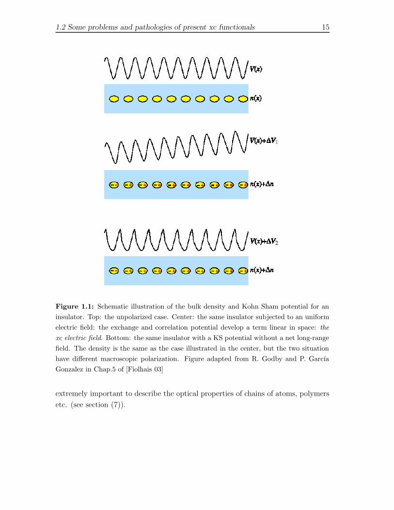
Figure 1.1: Schematic illustration of the bulk density and Kohn Sham potential for an
insulator. Top: the unpolarized case. Center: the same insulator subjected to an uniform
electric field: the exchange and correlation potential develop a term linear in space: the
xc electric field. Bottom: the same insulator with a KS potential without a net long-range
field. The density is the same as the case illustrated in the center, but the two situation
have different macroscopic polarization. Figure adapted from R. Godby and P. Garcıa
Gonzalez in Chap.5 of [Fiolhais 03]
extremely important to describe the optical properties of chains of atoms, polymers
etc. (see section (7)).

16 Chapter 1. Basic foundation of DFT
2 Time-dependent DFT (TDDFT)
2.1 Basic theorems
Time Dependent Density Functional Theory (TDDFT) is the extension of the DFT
to time dependent phenomena1. It permits calculation of excited states, but its
potentiality goes further because essentially it is at all effects an exact reformulation
of the time dependent Schrodinger equation and can be applied to describe in general
time-dependent phenomena beyond equilibrium. TDDFT is based on the Runge-
Gross theorem [Runge 84] that states:
• given a system of electrons prepared in a given initial sate |Φ(t0)〉, there is
a biunivocal correspondence between the external time-dependent potential
vext(r, t) and the time-dependent electron density n(r, t).
This is a generalization to time-dependent potentials and density, of the ordinary
DFT one-to-one correspondence:
n(r, t) ↔ v(r, t), (2.1)
Note that in this case:
• Two potentials are considered equivalent if they differ by any purely time-
dependent function.
• There is a dependence on the initial quantum state of the system.
• Contrary to intuition, the v-representability problem (the problem of the ex-
istence of a potential that produces a given density) is milder in the time-
dependent case than in the stationary case, and has been solved by van
Leeuwen [van Leeuwen 99] under a very broad assumptions for the initial state
of the system: moreover it gave an implicit form of constructing the vxc(r, t).
1 For a general overview see [Marques 06]
17
18 Chapter 2. Time-dependent DFT (TDDFT)
By virtue of the Runge Gross theorem, as in the static case, a fictitious Kohn-
Sham scheme can be introduced by considering a system of non-interacting electrons
subject to an external potential vKS(r, t) that reproduces the exact time dependent
density n(r, t) of the interacting system. The time-dependent density is obtained
propagating a set of a Schrodinger like equations, the time-dependent Kohn-Sham
equations (TDKS) where all the many-body effects are included through a time-
dependent exchange-correlation potential. This potential is unknown, and has to
be approximated in any practical application of the theory. The TDKS equations
looks like:
i∂
∂tϕi(r, t) =
[
− ∇2
2+ vKS[n](r, t)
]
ϕi(r, t) (2.2)
The density of the interacting system can be obtained from the time-dependent
Kohn-Sham orbitals:
n(r, t) =occ∑
i
|ϕi(r, t)|2. (2.3)
The Kohn-Sham potential is conventionally separated in the following way:
vks(r, t) = vext(r, t) + vH(r, t) + vxc(r, t) (2.4)
The first term is the external potential, the second term (Hartree potential) accounts
for the classical electrostatic interactions between electrons:
vH(r, t) =
∫
drn(r′, t)
|r− r′| (2.5)
The last term, the xc potential, includes all the non-trivial many body effects. In the
static case (DFT) the xc potentials is derived as a functional derivatives of the xc
energy Eq. (1.12), and it is not straightforward to extend such derivation in the time-
dependent case due to a problem of causality [Gross 95, Gross 96]. This problem has
been solved by Van Leeuwen [van Leeuwen 98], introducing a new action functional
A in the Keldish formalism. The time-dependent xc potential can be then written
as the functional derivative of the xc part of this action A.
vxc[n](r, t) =∂Axc
∂n(r, τ)
∣
∣
∣
n(r,t)(2.6)
where τ stands for the Keldish pseudo-time.
In any case the exact expression of vxc as a functional of the density is unknown and
the quality of any calculation will depend on the quality of the approximation of this
term. It is important to note that this is the only fundamental approximation in

2.2 Excitation energies in TDDFT 19
TDDFT. Before concluding this section we define the so-called exchange-correlation
kernel fxc:
fxc(r, r′, ω) =
δvxc[n(r, ω)]
δn(r′, ω)
∣
∣
∣
∣
∣
δvext=0
(2.7)
whose importance will be clear in the next session. In contrast with the ground state
DFT where very good xc potential exists, approximations to vxc(r, t) are still in their
infancy. Anyway the simplest approximations to the xc functional in TDDFT is the
adiabatic approximation, which use existing xc functionals for the ground state in
the time-dependent case. It consists in evaluating the ground state functional at
each time with the density n(r, t):
vadiabaticxc (r, t) = vxc[n](r)|n=n(t) (2.8)
where we have indicate with vxc an approximation to the ground state density xc
functional. Such time-dependent functional is of course local in time, ant this turns
to be a quite drastic approximation, and we expect to work only in the case where
the temporal dependence is small. In the case of the LDA , we obtain the so-called
Adiabatic Local Density Approximations (ALDA), that is one of the most widely
used functional that reads:
vALDAxc (r, t) = vHEGxc (n)|n=n(r,t) (2.9)
Of course the ALDA retains all the problems present in the LDA as for example the
wrong asymptotic behavior. In the ALDA, the fxc kernel is a contact function both
in time and space:
fALDAxc (r, t, r′, t′) = δ(t− t′)δ(r − r′)dvLDAxc (n)
dn
∣
∣
∣
n=n(r,t)(2.10)
Despite these problems, ALDA yields remarkably good results for finite systems
and has been used in some works discussed in this thesis. Of course there exist case
where such approximation dramatically fails and it is necessary to resort to much
more complicate functionals as in chapter (7). In particular the ALDA misses the
important 1/q2 divergence that controls the optical absorption of extended systems
with gap.
2.2 Excitation energies in TDDFT
In order to determine observable properties such as dynamical polarizability, ab-
sorption spectra and excitations energies, the fundamental quantity is the linear i
20 Chapter 2. Time-dependent DFT (TDDFT)
response of the electronic system, i.e. the response of the system when perturbed by
a weak time-dependent external electric potential δw(r, t). This perturbation will
induces a time-dependent perturbation of the density δn(r, t), that can be related
to the perturbing potential by:
δn(r, ω) =
∫
dr′χ(r, r′, ω)δw(r′, ω). (2.11)
where the function χ(r, r′, ω) 2 is the so called density-density response function.
The linear response of a molecule can be described via the dynamical polarizability
tensor i.e.:
δµi(ω) =∑
j
αij(ω)Ej(ω) (2.12)
where δµi(ω) =∫
drxiδn(r, ω) is the induced dipole in the i direction and Ej(ω) is
the external applied field. Assuming a dipolar perturbation, i.e. δv(r, ω) = −E(ω)·rthe polarizability tensor can be related to the response function by:
αij(ω) = −∫ ∫
drdr′xiχ(r, r′, ω)xj (2.13)
The imaginary part of the polarizability is then related to the photo-absorption cross
section σ(ω), the relevant magnitude measured in experiment, by:
σ(ω) =4πω
c
1
3=[Trα(ω)]. (2.14)
Now we illustrate how TDDFT allows to calculate the excited state energies of a
many body system, starting from the knowledge of the ground state of the system,
obtained for instance from a self-consistent DFT approach. The induced density of
Eq. (2.11) must be the same in the interacting and in the Kohn-Sham system, so
we can write the induced density δn(r, ω) as:
δn(r, ω) =
∫
dr′χKS(r, r′, ω)δvKS(r
′, ω). (2.15)
where δvKS includes the external potential and the induced Hartree potential and
the exchange and correlation potential. Such potential expressed in terms of the xc
kernel fxc (the functional derivative of the xc potential Eq. (2.7)) reads:
δvKS(r, ω) = δw(r, ω) +
∫
dr′δn(r′, ω)
|r − r′| +
∫
dr′fxc(r, r′, ω)δn(r′). (2.16)
2 For a time independent Hamiltonian the polarizability depend only on the time-differences and
a Fourier Transform in energy space can be easily performed

2.2 Excitation energies in TDDFT 21
The Kohn-Sham response function χKS(r, r′, ω) is the response function of a ficti-
tious non-interacting system, thus applying first order perturbation theory to KS
equations (1.16a), it can be expressed in terms of the ground state Kohn-Sham
eigenvalues εi and eigenfunctions ψi:
χKS(r, r′, ω) =
∑
ij
(fi − fj)ψi(r)ψ
∗j (r)ψj(r
′)ψ∗i (r
′)
ω − ωij + iη(2.17)
where ωij = (εi − εj) and fi is the occupation number of the Kohn-Sham orbitals.
Combining Eqs (2.11) and (2.15) we arrive at the Dyson equation for the interacting
response function:
χ(r, r′, ω) = χKS(r, r′, ω)+
∫
dr1r2χKS(r, r1, ω)[ 1
|r1 − r2|+fxc(r1, r2, ω)
]
χ(r2, r′, ω),
(2.18)
The solution of Eq. (2.18) provides in line of principle the exact full interacting
density response function: the poles of χ are the excitation energies of the system
as we will see below, so this equation allows to determine the exact excitation en-
ergies of the system once the Kohn-Sham χKS and the xc kernel fxc are known.
Here we note that with the approximation fxc = 0 we obtain the so called random
phase approximation (RPA) of the response function. In any case, a full solution
of Eq. (2.18) turns to be a difficult task from numerical point of view. Besides
the computational effort requires to solve the integral equation, it requires the non
interacting response function Eq. (2.17) that involve summations of both occupied
and unoccupied states, and such summations are sometimes slowly convergent, and
inclusion of a big amount of unoccupied states is required. In the following subsec-
tions we will describe the main ideas of the two different approaches to calculate
excitation energies that have been extensively used in the works reported in this
thesis: first we will present the matrix eigenvalue method that resort to the Linear
Response Theory, next we describe a method based in the full solution of the time
dependent Kohn-Sham equations Eq. (2.2).
2.2.1 Matrix eigenvalue method
A way to circumvent the difficulty of solving Eq. (2.18) for systems with discrete
spectrum such as molecules, starts by writing the Lehmann representation of the
interacting density response function:
χ(r, r′, ω) = limη→0+
∑
m
[〈0|n(r)|m〉〈m|n(r′)|0〉ω − (Em − E0) + iη
− 〈0|n(r)|m〉〈m|n(r′)|0〉ω + (Em − E0) + iη
]
(2.19)

22 Chapter 2. Time-dependent DFT (TDDFT)
where |m〉 and Em are the many body eigenstates and energies of the interacting
system and with |0〉 we have indicated the ground state. We see from Eq. (2.19)
that the density response function presents poles at the excitation energies of the
system ω = Ωm = Em − E0. This implies from Eq. (2.11) that also the induced
density has poles at the excitation energies Ωm because the external potential does
not have any special pole structure in function of ω. Looking at Eq. (2.17) we see
that the non-interacting Kohn-Sham response function has poles at the Kohn-Sham
eigenvalues differences ωij = εi− εj. From this consideration, rearranging Eq. (2.15)
and (2.16), one can derive the following eigenvalue equation [Petersilka 96]:
∫
dr′Ξ(r, r′, ω)ξ(r′, ω) = λ(ω)ξ(r, ω) (2.20)
where the kernel Ξ is defined as:
Ξ(r, r′, ω) = δ(r − r′) −∫
dsχKS(r, s, ω)[ 1
|s − r′| + fxc(s, r′, ω)
]
. (2.21)
Note that λ(ω) → 1 when ω coincide with the excitation energy Ω. Next, it is
possible to transform this eigenvalues equation, to another one whose eigenvalues
are true excitation energies [Jamorsky 96]. Expanding ξ(r, ω) in a basis set made of
products of occupied and unoccupied states we find the following matrix equation:
Θ(Ω) ~FI = Ω2 ~FI (2.22)
where the operator Θ(Ω) is given by:
Θijσ,klτ(Ω) = δσ,τ δi,kδj,lω2klτ + 2
√
(fiσ − fjσ)ωijσKijσ,klτ(Ω)√
(fkτ − flτ )ωklτ (2.23)
here the indexes (i, j) and (k, l) run over single particle orbitals, (σ, τ) are spin
indexes, and ωijσ = εjσ − εiσ. Note that here we have introduced the spin variables
in oder to treat also triplet excitations as will be discussed in chapter (7). The
Kernel Kijσ,klτ is given by:
Kijσ,klτ(Ω) =
∫
d3r
∫
d3r′ψ∗iσ(r)ψjσ(r)
[ 1
|r − r′| + fxc,στ (r, r′,Ω)
]
ψkτ (r′)ψ∗
lτ (r′)
(2.24)
Eq. (2.22) gives the exact position of the excitation energies Ω, and the corresponding
oscillator strengths are obtained from the eigenvectors of the operator Θ. It is
important to stress that the quality of the excitation energies will depend from the
truncation of the expansion, the used approximation for the unknown kernel fxc and

2.2 Excitation energies in TDDFT 23
for the exchange-correlation potential used for the calculation of the ground state
Kohn-Sham orbitals. The solution of Eq. (2.22) turns out to be computationally
really cumbersome, and it is possible to reduce such complexity paying the price of
loosing accuracy [Petersilka 96]. Assuming that the true excitation does not differ to
much from a single particle excitation it is possible to perform a Laurent expansion
of χKS around one particle energy difference between the Kohn-Sham eigenvalues
ωj0k0 = εk0 − εj0 :
χKS(r, r′, ω) = lim
η→0
ψj0(r)ψ∗j0(r
′)ψk0(r′)ψ∗
k0(r)
ω − ωj0k0 + iη+ higher orders. (2.25)
Neglecting the higher orders terms such approximation leads to the so-called Single
Pole Approximation (SPA):
Ω ' ωj0k0 +K(ωj0k0) (2.26)
where the term K for the singlet excitation 3 is given by:
K(ωj0k0) = 2<∫
dr
∫
r′ψj0(r)ψ∗j0
(r′)ψk0(r′)ψ∗
k0(r)[ 1
|r− r′| + fxc(r, r′, ωj0k0
)]
(2.27)
Here the term K can be viewed as a correction factor to the Kohn-Sham excitation
energies. Such approximation (SPA) although it is not precise as the full solution
of Eq. (2.22) provides a fast way to calculate excitation energies and turns to be a
very good approximation for many system as discussed in Refs.[Gonze 99, Appel 03].
From these considerations we can conclude that the crucial approximation for the
calculation of excited states in TDDFT is the choice of the static xc potential used
to calculate the Kohn-Sham eigenfunctions and eigenvalues. Moreover an important
feature of the calculation of excited states using the matrix eigenvalue method is
that it is possible to give a qualitative assignment of the character of the excited
state ΨI . Such assignment it is not possible solving directly the time dependent
Kohn-Sham equations, because as we will see in the next section, such method is
based on the time dependent density and no information on the wave functions is
available. If we first expand the excited state ΨI in single excited configurations as:
ΨI =
fiσ−fjσ>0∑
ijσ
cIijσa†jσaiσΦ + ..., (2.28)
3 Here we are considering a spin-unpolarized system. The extension to spin polarized systems
is straightforward, even if more complicated and the mixing of spin channel comes from the
exchange correlation kernel fxc,στ
24 Chapter 2. Time-dependent DFT (TDDFT)
assuming that the ground state wave function Ψ0 is a single determinant of Kohn
Sham orbitals and that matrix elements:
xijσ =
∫
ψiσ(r)xψjσ(r), (2.29)
are linearly independent, it is possible to calculate the coefficients of the expansion
in Eq. (2.28) by:
cIijσ =
√
εjσ − εiσΩI
F Iijσ. (2.30)
This expression, gives a weight of each single particle excitations that contribute to
a given excited state ΨI , and turn to be useful in order to assign a character to the
excitations, even if qualitative.
2.2.2 Full solution in real time of the TDDFT Kohn-Sham
equations
In order to calculate the linear and non-linear response functions of finite systems,
a very efficient method consists in the direct solution of the time dependent Kohn-
Sham equations Eq. (2.2). Such method was originally proposed to solve time
dependent Hartree Fock equations for studying nuclear reactions by Flocard and
coworkers [Flocard 78] and later has been used with success for TDDFT calculations
of photo-absorption for clusters [Yabana 96, Yabana 97, Yabana 99a, Yabana 99b,
Marques 01, Castro 02, Martinez 04] and biomolecules [Marques 03b, Varsano 05,
Tsolakidis 05]. Moreover this methods has been applied to study laser induced frag-
mentation problems and high harmonic generation [Castro 04b]. The starting point
for the solution of the time dependent problem is the initial state of the electronic
system: the Kohn-Sham ground state. Then we apply the external time-dependent
field and propagate the time-dependent KS equations following an unitary scheme
[Marques 03a, Castro 04c]. Then, in the particular case one is interested in obtain-
ing the linear optical absorption the system is instantaneously perturbed applying
a small electric field: δvext(r, t) = −k0xνδ(t) where xν = x, y, z. In this way all fre-
quencies of the system are excited with equal weight, and it is equivalent to give a
small momentum k0 to the electrons, so at the time 0+ the perturbed wave functions
are:
ψi(r, t = 0+) = eik0xνψi(r, 0) (2.31)

2.3 Dielectric Function 25
Where ψi(r, 0) is the ground state of the system. Next, the orbitals are propagated
in time:
ψi(r, t+ δt) = T exp
− i
t+δt∫
t
dthKS(t)
ψi(r, t) (2.32)
The absorption spectrum then can be calculated by Eqs.(2.13 and 2.14). Noticing
that the perturbation (a delta-function in real time) is a constant function in the
frequency domain, we can evaluate the polarizability as:
ανν(ω) = − 1
k0
∫
drxνδn(r, ω). (2.33)
In this expression δn(r, ω) is the Fourier transform of n(r, t) − n(r, 0) where n(r, 0)
is the ground-state density of the system. Of course according with Eq. (2.14) it is
necessary to calculate the polarizability for each spatial direction. With this time-
evolution scheme it is also possible to calculate circular dichroism for chiroptical
molecules, which is a very powerful tool used for characterization of biomolecules.
In order to do that the main quantity that has to be calculated is the rotatory
power strength function R(ω) = Rx(ω)+Ry(ω)+Rz(ω) that is obtained by Fourier
transform of the time evolution of the angular momentum operator:
Lν(t) =
occ∑
i
〈ψi| − i(r ×∇)ν|ψi〉. (2.34)
A great advantage of the time dependent scheme, as mentioned above, is that it
is not necessary an explicit calculation of unoccupied states, moreover it can be
extended to study non linear phenomena and it is also possible to perform nuclear
dynamics, eventually driven by high intensity laser fields [Castro 04b] to study laser
induced ionization and fragmentation problems.
2.3 Dielectric Function
We end this chapter giving the definition for extended systems of the dielectric
matrix and the screened coulomb potential that are key ingredient for the quasi-
particle and excitonic calculations that will be described in the next chapter. Here
we will give a description of these key-quantities starting from a density functional
approach, because it has been the starting point of all calculations performed in this
thesis. As described above, the response of the charge distribution of an electronic

26 Chapter 2. Time-dependent DFT (TDDFT)
system to an external perturbation δw(r, t) , is described in linear response theory,
by the full polarization function, χ(r, r′, ω), see Eq. (2.11). We have also defined
in Eq. (2.15) the polarization of an independent system (χKS)that link a change in
the electron density to a change in the total effective potential, that in the next we
indicate with χ0(r, r′, ω):
δn(r, ω) =
∫
dr′χ0(r, r′, ω)Vtot(r′, ω). (2.35)
In DFT framework, the independent particle polarization is accessible from the KS
eigenvalues and eigenfunction by Eq. (2.17) and the interacting and non-interacting
polarization functions, are connected by Dyson-like equation Eq. (2.18), that written
in matrix formalism reads:
χ =[
1 − χ0(v + fxc)]−1
χ0 (2.36)
In connection with classical electrodynamics we define the inverse dielectric function
as a measure of the screening in the system through the ratio between the total and
applied potentials:
ε−1(r, r′, ω) =δVtot(r, ω)
δw(r′, ω)(2.37)
In order to relate the dielectric function to the microscopic polarizability we consider
now a test particle as a probe. The induced charge create a screening and the probe
will be only affected by the electrostatic Hartree variation in Eq. (2.16), i.e.:
δVtot(r, ω) = δw(r, ω) +
∫
dr′δn(r′, ω)v(r, r′), (2.38)
where with v(r, r′) we have indicated the coulomb potential. Now we can easily
relate the dielectric matrix to the polarizability by:
ε−1(r, r′, ω) = δ(r − r′) +
∫
dr′v(r, r′)χ(r, r′, ω) (2.39)
Once introduced the inverse dielectric matrix ε−1(r, r′), it is useful to define the
dynamically screened Coulomb interaction W :
W (r, r′, ω) =
∫
dr1v(r, r1)ε−1(r1, r
′, ω) (2.40)
The interaction function W, take into account the screening and, as we will see
later, is a key quantity for quasiparticle and excitonic calculations. Now we can
introduce the so called Random Phase Approximation (RPA), that is obtained by
2.3 Dielectric Function 27
setting the exchange correlation contribution to χ equal to zero in Eq. (2.36). So in
this approximation the dielectric function is obtained by:
ε−1RPA =1 + v(1 − χ0v)−1χ0 (2.41a)
εRPA =1 − vχ0 (2.41b)
The Random Phase Approximation is widely used and we have made extensive use of
it for the calculation of the screened potential. The dielectric function ε−1(r, r′, ω), is
a microscopic quantity and in order to relates it to measurable quantities, spatial av-
erages have to be performed. In the case of solids, following Refs.[Adler 62, Wiser 63]
the macroscopic dielectric function is related to the inverse of the microscopic di-
electric matrix by:
εM(ω) = limq→0
1
ε−1G,G′(q, ω)
∣
∣
∣
G=G′=0(2.42)
where we have expressed the microscopic dielectric in momentum space, which is
related to real space by a Fourier transform:
ε−1(r, r′, ω) =1
(2π)3
∫
Bz
dq∑
G,G′
ei(q+G)·rε−1G,G′(q, ω)e−i(q+G)·r (2.43)
where q lies in the first Brillouin zone and G are reciprocal lattice vectors. Here we
note that Eq. (2.42) requires an inversion of the microscopic dielectric matrix and in
general differs from limq→0 ε0,0(q, ω). The discrepancy between these two quantity
is called Local Field Effect. The local field effects take into account microscopic
fluctuations induced at atomic scale that arise for the inhomogeneity of the system.
The macroscopic dielectric function is then linked to the measurable absorption
spectra (ABS) and electron energy loss spectra (EELS) by [Grosso 00]:
ABS ≡ =[εM ] (2.44a)
EELS ≡ −=[1
εM] (2.44b)
Note that for finite system we have that absorption spectra is proportional to the
dynamical polarizability as seen in Eq. (2.14) and imaginary part of the dielectric
function and the loss function coincide [Sottile 05].

28 Chapter 2. Time-dependent DFT (TDDFT)
3 Many Body Perturbation
Theory
The KS-DFT scheme, as presented in the previous chapter, provides very good
results for the ground state properties of a huge class of system, but it has also
drawbacks: as seen in section (1.2.1), the eigenvalues obtained from the solution of
the KS equations, except for the highest occupied, does not have a physical mean-
ings, and when used to calculate gaps of semiconductor or insulator the results are
extremely poor, the gaps are underestimated and the quality of the band structures
depends strongly on the studied material. In order to obtain physical meaningful
gaps we have to go beyond the the DFT scheme and to resort to the quasipar-
ticle (QP) concepts. The quasiparticle energies are given by the energy needed
to add (remove) an electron to the system and are experimentally accessible from
direct or inverse photo-emission experiments. In this chapter we will briefly de-
scribe this concepts by the Many Body Perturbation Theory (MBPT), introducing
the Green Function formalism, the Self Energy concept and the GW approximation,
and we remind the reader to the following books and article of many particle physics
[Fetter 81, Hedin 69, Gross 91] for a deeper discussions. Then in section (3.4) we
will see how to include the electron-hole attraction effects in the macroscopic dielec-
tric function going beyond the GW approximation. Last, in section (3.5) we will
combine the MBPT with the TDDFT for obtaining an exchange-correlation kernel
that includes both the quasiparticle energies and the electron-hole attraction effects
that has been extensively used chapter (7).
3.1 Quasiparticle formulation
In section (1) we have seen that in the Kohn-Sham scheme the response of a system
of interacting electrons to an external potential is mapped into a system of non-
interacting electrons responding to an effective potential (KS potential). In Many
Body Perturbation Theory we start from the idea that an electron in an interacting
29
30 Chapter 3. Many Body Perturbation Theory
system perturbs the particles in its proximity and can be tough as a particle moving
through the system, surrounded by a cloud of other particles that are being pushed
out of the way or dragged along by its motions, so that the entire entity moves
like a weekly interacting particle. The entity particle plus screening cloud is called
quasiparticle. So, similarly as the Kohn-Sham scheme, the interacting “bare” particle
problems can be described via weakly interacting quasiparticles as they interact
via a screened potential rather than the bare coulomb potential. The advantage
of such description permits to perform a perturbative expansion with respect the
quasiparticle interaction. Note that the quasiparticles states are not eigenstates of
the N-body Hamiltonian and therefore they have a finite lifetime.
One particle Green’s function
The quantity that describe the propagation of one particle through the system is the
one particle Green’s function. It contains the information on energy and lifetimes
of the quasiparticle, and also on the ground state energy of the system and the
momentum distribution. The one particle Green’s function is defined as:
G(x1, t1,x2, t2) = −i〈ΨN |T [ψH(x1, t1)ψ†H(x2, t2)]|ΨN〉, (3.1)
Here we use the abbreviation x = (x, t) = (r, σ, t). ΨN is the Heisenberg ground
state vector of the interacting N-electron system satisfying the Schrodinger equation
H|ΨN〉 = E|ΨN〉, ψH and ψ†H are respectively the annihilation and creation field
operator and T is the Wick time ordering operator. Explicitly:
ψH(x, t) =eiHtψ(x)e−iHt (3.2a)
ψ†H(x, t) =e−iHtψ†(x)eiHt (3.2b)
and the field operator satisfy the anti-commutation relation:
ψH(x), ψ†H(x′)
=δ(x− x′) (3.3a)
ψH(x), ψH(x′)
=
ψ†H(x), ψ†
H(x′)
= 0 (3.3b)
and:
T [ψH(x1, t1)ψ†H(x2, t2)] =
ψH(x1, t1)ψ†H(x2, t2) if t1 > t2
−ψH(x2, t2)ψ†H(x1, t1) if t1 < t2
(3.4)

3.1 Quasiparticle formulation 31
The Hamiltonian H = T + W + V of Eq. (1.1) in the second quantization formalism
now reads:
T =
∫
dxψ†H(x)
[
− 1
2∇2
r
]
ψH(x) (3.5a)
W =
∫
dxψ†H(x)w(x)ψH(x) (3.5b)
V =1
2
∫
dxdx′ψ†H(x)ψ†
H(x′)v(r, r′)ψH(x′)ψH(x) (3.5c)
From this definition we can see that the Green function G(x1, x2) describes the
probability amplitude for the propagation of an electron (hole) from position r2 at
t2 to r1 at time t1 for t1 > t2 (t1 < t2). If now we introduce the complete set of the
eigenstates of the Hamiltonian H, for the (N+1) and (N-1) particle systems and we
perform a Fourier transform in energy space we obtain:
G(x1,x2;ω) =∑
s
fs(x1)f∗s (x2)
ω − εs + iηsgn(εs − µ)(3.6)
where µ is the chemical potential,
εs =
E(N+1)s − E
(N)N for εs ≥ µ
E(N)N − E
(N−1)s for εs < µ
(3.7)
where for the total energies we have used the notation of section (1.2.1) and with
the subscript s we indicate the quantum label of the states of the N+1 (N-1) system.
The amplitudes fs(x) are defined as:
fs(x) =
〈ΨN |ψ(x)|ΨN+1,s〉 for εs ≥ µ
〈ΨN−1,s|ψ(x)|ΨN〉 for εs < µ(3.8)
We see from the expression (3.6) that the Green function has the poles at the electron
addition (removal) energies and describes quasiparticle excitations. By taking the
imaginary part of Eq. (3.6) we have the so-called spectral function:
A(x1,x2;ω) =1
π|=G(x1,x2;ω)| =
∑
s
fs(x1)f∗s (x2)δ(ω − εs) (3.9)
A(x1,x2;ω) is a superposition of delta functions with weights given by the ampli-
tudes fs(x) centered at each of the one particle excitation energies εs. In the cases
where an appreciable fraction of the weight spectral function A(x1,x2;ω) goes into
32 Chapter 3. Many Body Perturbation Theory
µεniεqpεsat
A(ω
) interacting
non interacting
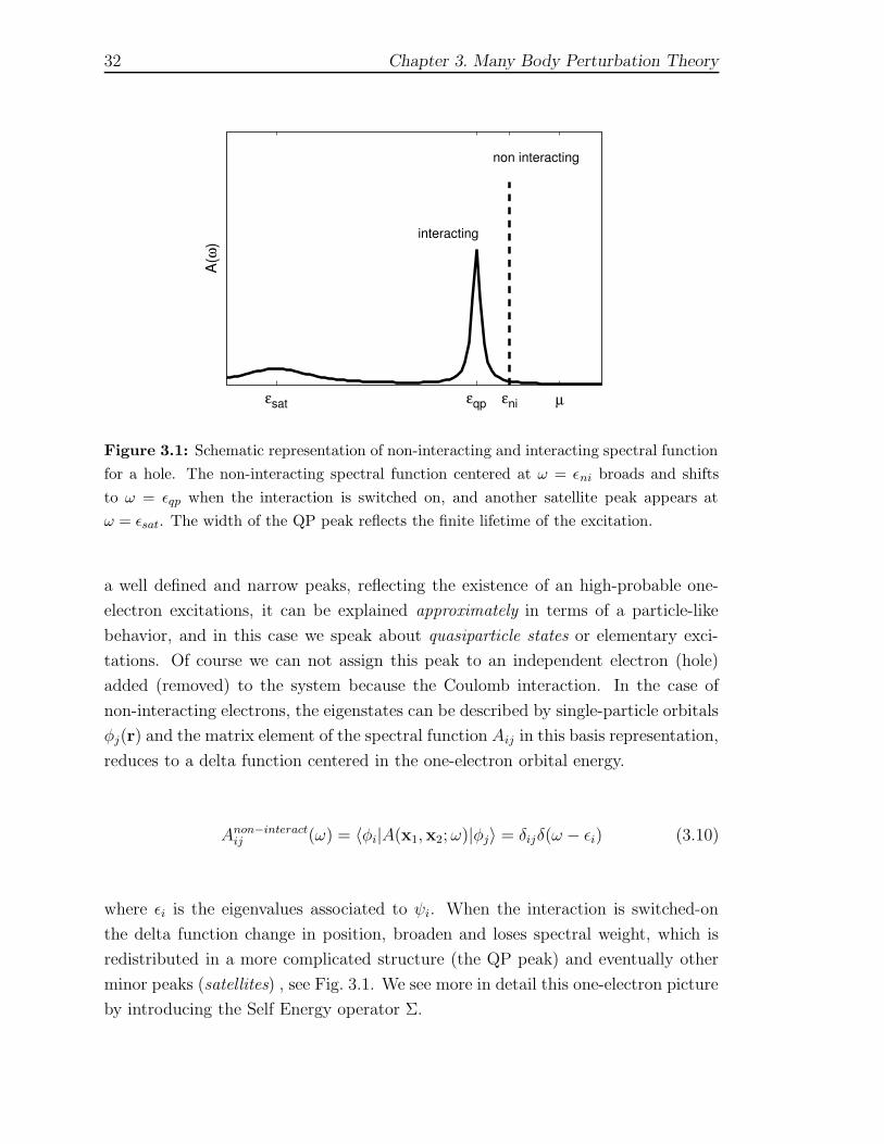
Figure 3.1: Schematic representation of non-interacting and interacting spectral function
for a hole. The non-interacting spectral function centered at ω = εni broads and shifts
to ω = εqp when the interaction is switched on, and another satellite peak appears at
ω = εsat. The width of the QP peak reflects the finite lifetime of the excitation.
a well defined and narrow peaks, reflecting the existence of an high-probable one-
electron excitations, it can be explained approximately in terms of a particle-like
behavior, and in this case we speak about quasiparticle states or elementary exci-
tations. Of course we can not assign this peak to an independent electron (hole)
added (removed) to the system because the Coulomb interaction. In the case of
non-interacting electrons, the eigenstates can be described by single-particle orbitals
φj(r) and the matrix element of the spectral function Aij in this basis representation,
reduces to a delta function centered in the one-electron orbital energy.
Anon−interactij (ω) = 〈φi|A(x1,x2;ω)|φj〉 = δijδ(ω − εi) (3.10)
where εi is the eigenvalues associated to ψi. When the interaction is switched-on
the delta function change in position, broaden and loses spectral weight, which is
redistributed in a more complicated structure (the QP peak) and eventually other
minor peaks (satellites) , see Fig. 3.1. We see more in detail this one-electron picture
by introducing the Self Energy operator Σ.

3.1 Quasiparticle formulation 33
The Self-Energy Σ
An implicit definition of Σ can be given from the equation of motion of the one
particle Green’s function which involves the two-particle Green’s function [Hedin 69].
The self-energy allows to close formally the hierarchy of equations of motion of higher
order Green functions. We introduce the Self Energy through the Dyson equation:
G(x1, x2) = GH(x1, x2) +
∫
dx3dx4GH(x1, x3)Σ(x3, x4)G(x4, x2) (3.11)
where GH is the Hartree Green function of the non-interacting system, solution of
the equation:[
ω − h0(x1)]
GH(x1,x2;ω) = δ(x1 − x2) (3.12)
here h0(x) is the one-electron Hamiltonian: h0(x) = −∇2r/2+w(x)+VH(x) under the
total average potential (external potential plus classical Hartree potential). From
Eqs (3.11) and (3.12) it is clear that the operator Σ contain all the exchange and
correlation many body effects:
[
ω − h0(x1)]
G(x1,x2;ω) = δ(x1 − x2) +
∫
dxΣ(x1,x;ω)G(x,x2;ω) (3.13)
The complicate many-body character of the Green-s function G arise from the En-
ergy dependence in Eq. (3.13). Expressing the Green function in a base of energy
dependent wave functions φi(x, ω), that form an orthonormal and complete set for
each ω as:
G(x1,x2) =∑
i
φi(x1, ω)φ∗i (x2, ω)
ω − Ei(ω)(3.14)
provided that the complex wave-functions φi(x, ω) and energies Ei(ω) are solution
of the equation:
h0(x)φi(x, ω) +
∫
dx′Σ(x,x′;ω)φi(x′, ω) = Ei(ω)φi(x, ω) (3.15)
Because Σ is a non-hermitian operator the energies Ei(ω) are in general complex
and the imaginary part gives the lifetime of the excitation. If the energy spectrum
presents sharp peaks as illustrated in the previous paragraph Ei(ω) ' EQPi we arrive
at the quasiparticle equation:
h0(x)φQPi (x) +
∫
dx′Σ(x,x′;EQPi )φQPi (x′) = EQP
i φQPi (x) (3.16)
We can see from this equation that the qp-equation has a resemblance to the KS
equation (1.16a) where the non local and energy dependent Self Energy Σ plays
34 Chapter 3. Many Body Perturbation Theory
the role of the exchange and correlation potential vxc, but while the xc potential
is part of the potential of the fictitious non interacting system, Σ may be tough as
the potential felt by an added (removed) electron to (from) the interacting system.
From the solution Eq. (3.16) , expanding Σi(ω) = 〈φQPi |Σ(ω)|φQPi around the value
ω = EQP we can calculate the Green function and the spectral function (3.9) as:
Gi(ω) = 〈φQPi |G(ω)|φQPi 〉 ' Zi
ω −(
<(EQPi ) − i=(EQP
i )) (3.17)
where Zi is the so-called renormalization factor defined as:
Z−1i = 1 − ∂Σi(ω)
∂ω
∣
∣
∣
ω=EQPi
(3.18)
and gives the portion of the spectral weight under the quasiparticle peak. We see
that if =(EQPi ) is small the spectral function will present a well defined peak centered
around <(EQPi ).
3.2 Hedin’s Equations
Until now we have seen how it is possible to calculate energy and lifetimes of quasi-
particle excitation solving Eq. (3.16). Of course before that we have to know how
is made the operator Σ, that have of course be approximated. The Many Body
Perturbation Theory gives us a practical scheme in order to solve such task. As
perturbation we will not consider the bare coulomb potential, V , but results more
natural to consider the screened coulomb potential W introduced in Eq. (2.40) that
has reduced strength with respect the bare potential, and we will write the Self En-
ergy as a perturbation series in terms of W . A systematic way to construct exactly
Σ was proposed by Hedin [Hedin 65, Hedin 69] and consists of a set of five Dyson
like equations:
P (12) = − i
∫
d(34)G(13)G(41+)Γ(34, 2) (3.19a)
W (12) =V (12) +
∫
d(34)W (13)P (34)V (4, 2) (3.19b)
Σ(12) =i
∫
d(34)G(14)W (1+3)Γ(42, 3) (3.19c)
G(12) =G0(12) +
∫
d(34)G0(13)Σ(34)G(42) (3.19d)
Γ(12, 3) =δ(12)δ(13) +
∫
d(4567)∂Σ(12)
∂G(45)G(46)G(75)Γ(67, 3) (3.19e)

3.3 The GW approximation 35
where we used the notation 1 ≡ (x1, t1). Above P is the irreducible polarization
function, Γ is the so called vertex function and G0 coincide with the Hartree Green
function (see Eq. (3.11)) Note here that the irreducible polarization function P
, represents the variation of the induced density with respect to a variation of a
classical total potential (external plus Hartree) and differs from the polarization
function defined in section (2.3) 1 and it is related to the dielectric function by 2:
ε(12) = δ(12) −∫
d(3)V (13)P (32) (3.20)
We can here recognize that if we consider Σ = 0 in Eq. (3.19e), we get P 0(12) =
−iG0(12)G0(21+), in this case P 0 and χ0 coincide and Eq. (3.20) is the RPA dielec-
tric function of Eq. (2.41b).
3.3 The GW approximation
A method to solve this set of equation was proposed by Hedin, by starting the
iterative solution starting Σ = 0 (Hartree approximation). This approximations
yields to Γ(12, 3) = δ(12)δ(13). The others expressions of Eq. (3.19) becomes in
first iteration:
P 0(12) = − iG0(12)G0(21+) (3.21a)
W 0(12) =V (12) +
∫
d(34)W 0(13)P 0(34)V (4, 2) (3.21b)
Σ(12) =iG0(12)W 0(1+2) (3.21c)
The GW approximation 3 consists in stopping at the first step of the iteration, so
in neglecting the vertex function and calculating the Σ by Eq. (3.21) and then solve
the quasiparticle equation (3.16). Substantially from Eq. (3.21) we can recognize
that G0 is just the Hartree Green’s function, the polarizability P 0 is the independent
particle polarization and gives the Adler Wiser polarization function, W 0 is the RPA
1 In Eq. (2.11) we have defined the reducible response, i.e. the variation of the induced density
with respect the variation of the external field.2 Note that Eq. (3.19b) can be written as: W = ε−1V linking the screened Coulomb to the bare
Coulomb.3 Here we describe the non self-consistent GW approximation, that is the approach we have
adopted in this thesis. For a general overview on the GW approximation see:[Aryasetiawan 98,
Aulbur 00a]
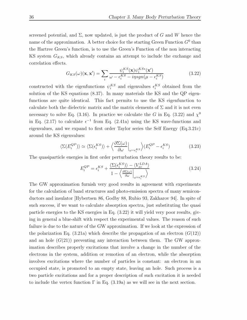
36 Chapter 3. Many Body Perturbation Theory
screened potential, and Σ, now updated, is just the product of G and W hence the
name of the approximation. A better choice for the starting Green Function G0 than
the Hartree Green’s function, is to use the Green’s Function of the non interacting
KS system GKS, which already contains an attempt to include the exchange and
correlation effects.
GKS(ω)(x,x′) =∑
i
ψKSi (x)ψKS∗i (x′)
ω − εKSi − iηsgn(µ− εKSi )(3.22)
constructed with the eigenfunctions ψKSi and eigenvalues εKSi obtained from the
solution of the KS equations (8.37). In many materials the KS and the QP eigen-
functions are quite identical. This fact permits to use the KS eigenfunction to
calculate both the dielectric matrix and the matrix elements of Σ and it is not even
necessary to solve Eq. (3.16). In practice we calculate the G in Eq. (3.22) and χ0
in Eq. (2.17) to calculate ε−1 from Eq. (2.41a) using the KS wave-functions and
eigenvalues, and we expand to first order Taylor series the Self Energy (Eq.3.21c)
around the KS eigenvalues:
〈Σ(EQPi )〉 ' 〈Σ(εKSi )〉 +
⟨∂Σ(ω)
∂ω
∣
∣
∣
ω=εKSi
⟩
(EQPi − εKSi ) (3.23)
The quasiparticle energies in first order perturbation theory results to be:
EQPi = εKSi +
〈Σ(εKSi )〉 − 〈V LDAxc 〉
1 −⟨
∂Σ(ω)∂ω
∣
∣
∣
ω=εKSi
⟩ (3.24)
The GW approximation furnish very good results in agreement with experiments
for the calculation of band structures and photo-emission spectra of many semicon-
ductors and insulator [Hybertsen 86, Godby 88, Rubio 93, Zakharov 94]. In spite of
such success, if we want to calculate absorption spectra, just substituting the quasi
particle energies to the KS energies in Eq. (3.22) it will yield very poor results, giv-
ing in general a blue-shift with respect the experimental values. The reason of such
failure is due to the nature of the GW approximation. If we look at the expression of
the polarization Eq. (3.21a) which describe the propagation of an electron (G(12))
and an hole (G(21)) preventing any interaction between them. The GW approx-
imation describes properly excitations that involve a change in the number of the
electrons in the system, addition or remotion of an electron, while the absorption
involves excitations where the number of particles is constant: an electron in an
occupied state, is promoted to an empty state, leaving an hole. Such process is a
two particle excitations and for a proper description of such excitation it is needed
to include the vertex function Γ in Eq. (3.19a) as we will see in the next section.
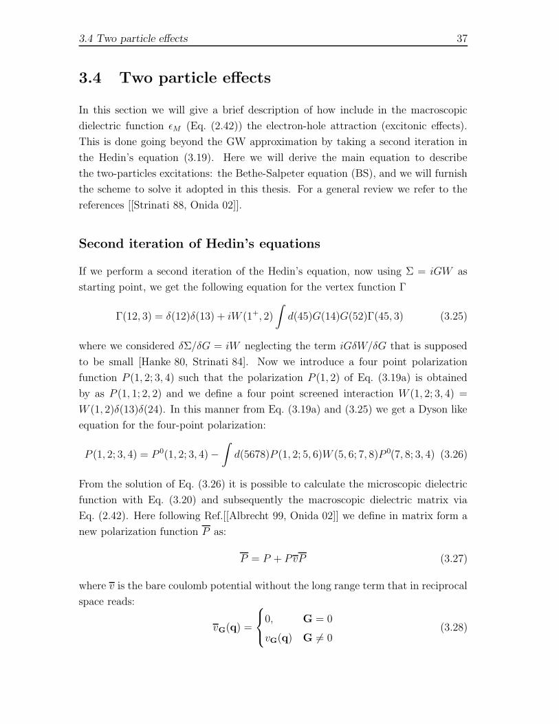
3.4 Two particle effects 37
3.4 Two particle effects
In this section we will give a brief description of how include in the macroscopic
dielectric function εM (Eq. (2.42)) the electron-hole attraction (excitonic effects).
This is done going beyond the GW approximation by taking a second iteration in
the Hedin’s equation (3.19). Here we will derive the main equation to describe
the two-particles excitations: the Bethe-Salpeter equation (BS), and we will furnish
the scheme to solve it adopted in this thesis. For a general review we refer to the
references [[Strinati 88, Onida 02]].
Second iteration of Hedin’s equations
If we perform a second iteration of the Hedin’s equation, now using Σ = iGW as
starting point, we get the following equation for the vertex function Γ
Γ(12, 3) = δ(12)δ(13) + iW (1+, 2)
∫
d(45)G(14)G(52)Γ(45, 3) (3.25)
where we considered δΣ/δG = iW neglecting the term iGδW/δG that is supposed
to be small [Hanke 80, Strinati 84]. Now we introduce a four point polarization
function P (1, 2; 3, 4) such that the polarization P (1, 2) of Eq. (3.19a) is obtained
by as P (1, 1; 2, 2) and we define a four point screened interaction W (1, 2; 3, 4) =
W (1, 2)δ(13)δ(24). In this manner from Eq. (3.19a) and (3.25) we get a Dyson like
equation for the four-point polarization:
P (1, 2; 3, 4) = P 0(1, 2; 3, 4)−∫
d(5678)P (1, 2; 5, 6)W (5, 6; 7, 8)P 0(7, 8; 3, 4) (3.26)
From the solution of Eq. (3.26) it is possible to calculate the microscopic dielectric
function with Eq. (3.20) and subsequently the macroscopic dielectric matrix via
Eq. (2.42). Here following Ref.[[Albrecht 99, Onida 02]] we define in matrix form a
new polarization function P as:
P = P + PvP (3.27)
where v is the bare coulomb potential without the long range term that in reciprocal
space reads:
vG(q) =
0, G = 0
vG(q) G 6= 0(3.28)

38 Chapter 3. Many Body Perturbation Theory
It can be demonstrated [Albrecht 99] that this new polarization function P is related
to the macroscopic dielectric function by:
εM(ω) = 1 − limq→0
[v0(q)P 00(q, ω)] (3.29)
or equivalently:
εM(ω) = 1 − limq→0
[
v0(q)
∫
drdr′e−iq·(r−r′)P (r, r, r′, r′;ω)]
(3.30)
Inserting Eq. (3.26) in Eq. (3.27) we obtain the so-called Bethe Salpeter Equation
(BS) that in matrix form reads::
P = P 0 + P 0KP (3.31)
The Kernel K of the BS equation:
K(1, 2; 3, 4) = −iδ(1, 2)δ(3, 4)v(1, 3) + iδ(1, 3)δ(2, 4)W (1, 2) (3.32)
is composed of two terms: The first one is called the exchange term, while the second
one, that is the variation of the Self energy with respect the single particle Green’s
function is called direct-term. In the GW approximation it is the screened coulomb
potential. We note here that if we replace the screened coulomb potential by the
bare coulomb potential, the BS equation reduces to the time dependent Hartree
Fock equation.
Effective two particle equation
In the last section we have shown how to include the electron-hole attraction in the
macroscopic dielectric function, introducing a four point polarizability that could
be calculated solving the Dyson-like equation Eq. (3.31) through an inversion. This
is a very cumbersome procedure, so here, we show how to reduce the calculation
of the 4-point polarization function to an effective eigenvalue problem to be solved
by diagonalization. The main idea is to use a basis of KS Bloch function pairs
φn1(r)φn2(r) and use the spectral representation for the inversion. First of all we
consider the propagation and the interaction of the two particle simultaneous and
instantaneous. In this way we reduce the four time coordinate to just one. In the
next we will use the notation x1 → r1, σ1, so the time coordinate it is not included
anymore in the index, and performing a Fourier Transform in energy space we will
3.4 Two particle effects 39
have P (1, 2; 3, 4) → P (x1,x2;x3,x4|ω). The change of basis in transition space is
performed by the relation:
P (n1,n2)(n3,n4) =
∫
dx1dx2dx3dx4P (x1,x2;x3,x4)φn1(x1)φ∗n2
(x2)φ∗n3
(x3)φn4(x4)
(3.33)
In the transition space the non-interacting polarizability reads:
P 0(n1,n2)(n3,n4)
=(fn2 − fn1)δn1,n3δn2,n4
εn2 − εn1 − ω − iη(3.34)
where with fn we have indicate the occupation number and η is a positive infinites-
imal. Now we define the excitonic Hamiltonian as:
Hexc(n1,n2)(n3,n4) = (εn2 − εn1)δn1,n3δn2,n4 + i(fn2 − fn1)K(n1,n2)(n3 ,n4) (3.35)
from Eq. (3.31) can be shown that the polarizability P can be expressed as:
P (n1,n2)(n3,n4) =[
Hexc − Iω]−1
(n1,n2)(n3 ,n4)(fn4 − fn3) (3.36)
where I is the identity matrix I = δn1,n3δn2,n4. In order to solve the inversion we use
the spectral representation, namely:
[
Hexc − Iω]−1
=∑
λ,λ′
|λ〉S−1λ,λ′〈λ′|
Eλ − ω(3.37)
where with |λ〉 and Eλ we have indicated the eigenvalues and eigenvector of H exc:
Hexc|λ〉 = Eλ|λ〉 (3.38)
and Sλ,λ′ is the overlap matrix:
Sλ,λ′ = 〈λ′|λ〉 (3.39)
Note that Eq. (3.37) holds for a general non Hermitian matrix. Explicitly we have
defined an effective two-particle Schrodinger equation:
Hexc(n1,n2)(n3,n4)
A(n3,n4)λ = EλA
(n1,n2)λ (3.40)
that can be solved by diagonalization. This equation couples the different two
particle configurations and the coefficients A(n1,n2)λ of the state |λ〉 permits to identify
the character of each excitation. The exciton amplitude is given by:
Ψλ(x1,x2) =∑
n1,n2
A(n1,n2)λ φ∗
n1(x1)φn2(x2) (3.41)
40 Chapter 3. Many Body Perturbation Theory
Moreover from the eigenvectors and eigenvalues of Eq. (3.40) we can calculate from
Eqs.(3.29),(3.36), (3.37) the macroscopic dielectric matrix by:
εM (ω) = 1 − limq→0
v0(q)∑
λ,λ′
[
∑
n1,n2
〈n1|e−iq·r|n2〉A
(n1,n2)λ
Eλ − ω − iη×
× S−1λ,λ′
∑
n3,n4
〈n3|eiq·r|n4〉A∗(n3,n4)λ (fn4 − fn3)
]
(3.42)
Structure of the Excitonic Hamiltonian
In this section we examine the structure of the excitonic Hamiltonian Eq. (3.35)
more in detail. We indicate with the letter v and c respectively the occupied and
empty states and we omit the index k associated to the vertical transition vk → ck
that have to be considered when solids are studied. Eq. (3.35) has the following
structure:
Hexc =
v′c′ c′v′ v′v′ c′c′vc Hexc,res
(vc)(v′c′) K(vc)(c′v′) K(vc)(v′ v′ K(vc)(c′ c′
cv −[K(vc)(c′v′)]∗ −[Hexc,res
(vc)(v′c′)]∗ −K(cv)(v′ v′) −K(cv)(c′ c)′
vv 0 0 (εv − εv)δv,v′δv,v′ 0
cc 0 0 0 (εc − εc)δc,c′δc,c′
From Eq. (3.36) it can be shown that not all the terms contribute to the macroscopic
dielectric function, and the relevant part of the excitonic Hamiltonian reduces to only
the terms between occupied and unoccupied pairs:
Hexc =
Hexc,res(v,c)(v′ ,c′) Kcoupl
(v,c)(c′,v′)
−[Kcoupl(v,c)(c′ ,v′)]
∗ −[Hexc,res(v,c)(v′ ,c′)]
∗
(3.43)
The two diagonal blocks involves only positive and negative frequency transitions
and are called respectively resonant and anti-resonant parts, while the off-diagonal
block mix positive and negative transition and we call them coupling part. From
Eq. (3.35) and Eq. (3.32) we can write the different terms of the Hamiltonian ex-
plicitly. We split the resonant part in three terms:
Hexc,res(v,c)(v′ ,c′) = Hdia
(v,c)(v′ ,c′) +Kx(v,c)(v′ ,c′) +Kd
(v,c)(v′ ,c′) (3.44)

3.4 Two particle effects 41
hv hv hv
v vv
c c
c
ωcv
ωω
cv
cv
W
GW BSE
excEb
Independent particles
Figure 3.2: Schematic representation of the excitations and interactions for an absorption
process: Left panel DFT independent particles levels. Central panel: GW band structure,
the gap is well estimated, but the absorption spectrum is blue-shifted. Right panel: BS:
electron-hole attraction included and formation of a bound exciton.
that have the forms:
Hdia(v,c)(v′ ,c′) = (εc − εv)δvv′δcc′ (3.45a)
Kx(v,c)(v′ ,c′) =
∫
dx
∫
dx′φ∗c(x)φv(x)
1
|r− r′|φc′(x′)φ∗
v′(x′) (3.45b)
Kd(v,c)(v′ ,c′) = −
∫
dx
∫
dx′φ∗c(x)φc′(x)
∫
dr1ε−1(r, r1)
1
|r1 − r′|φv(x′)φ∗
v′(x′)
(3.45c)
In the diagonal term the independent-particle energies ε are the quasiparticle en-
ergies from a GW calculation. In the direct term Kd the dynamical effects in
the screening are neglected, and the static dielectric matrix is calculated in RPA
framework Eq. (2.41a). With Kx we have indicated the so-called exchange term. 4
Similarly the coupling term can be split as:
Kcoupl(v,c)(c′,v′) = Kx
(v,c)(c′,v′) +Kd(v,c)(c′,v′) (3.46)
Looking at the structure of each term results that the resonant part itself is an Her-
mitian matrix: (Hexc,res)∗ = (Hexc,res)T , while the coupling part alone is symmetric:
4 In section (5.4.5) we will derive a similar expression of the Hamiltonian, for the TDDFT, anyway
the two equation have a different structure due to the change in the indexes vc′ → c′v in
the direct term.

42 Chapter 3. Many Body Perturbation Theory
Kcoupl = (Kcoupl)T . Until now we do not have included the spin structure of the of
the BS. Under the assumption that the spin-orbit interaction is negligible compared
with the electron-hole interaction, we can classify the single-particle states as spin-up
and spin-down states. Within this assumption the electron-hole pair space until now
indicated as vc consists of four subspace:v ↑ c ↑,v ↑ c ↓,v ↓ c ↑,v ↓ c ↓. If
now we look at the excitonic Hamiltonian in this subspace we obtain from Eq. (3.45)
for the resonant part:
Hexcres =
v′ ↑ c′ ↑ v′ ↑ c′ ↓ v′ ↓ c′ ↑ v′ ↓ c′ ↓v ↑ c ↑ Hdia +Kd +Kx 0 0 Kx
v ↑ c ↓ 0 Hdia +Kd 0 0
v ↓ c ↑ 0 0 Hdia +Kd 0
v ↓ c ↓ Kx 0 0 Hdia +Kd +Kx
So in the assumption of weak spin-orbit interaction this Hamiltonian can be decou-
pled into spin-singlet solutions and spin-triplet solutions, and the BS can be solved
separately:
Singlet 1√2(v ↑ c ↑ −v ↓ c ↓) Hexc = Hdia +Kd + 2Kx
Triplet
v ↑ c ↑v ↓ c ↓1√2(v ↑ c ↑ +v ↓ c ↓)
Hexc = Hdia +Kd
(3.47)
In the same manner we obtain for the coupling part:
Kcoupl,singlet(v,c)(c′,v′) =Kd
(v,c)(c′,v′) + 2Kx(v,c)(c′,v′)
Kcoupl,triplet(v,c)(c′ ,v′) =Kd
(v,c)(c′,v′)
Of course in the cases where the spin-orbit coupling cannot be neglected the clas-
sification of the single state in spin-up spin-down states is not valid anymore. The
singlet and triplet configurations are mixed and the full spin structure have to be
included in the Bethe-Salpeter Hamiltonian, but it is not the case for the systems
treated in this thesis. We see that the exchange term Kx that involve the bare
Coulomb potential Eq. (3.32) controls the splitting between spin-singlet and spin-
triplet excitations. The direct term Kd involve the screened Coulomb interaction
W produces the attractive electron-hole interaction and is the responsible for the
formation of bound electron-hole states, called excitons. In Fig(3.2) are sketched the
energy levels and interactions passing from the DFT calculation to the BS solutions
through the GW approximations for the quasiparticle energies.
3.5 Combining MBPT and TDDFT 43
3.5 Combining MBPT and TDDFT
The solution of the Bethe Salpeter equation described above reproduces very well
the experimental spectra of semiconductor and insulator. However looking at the
excitonic matrix we see that the dimension of the matrix increases with the number
of the valence and conduction band, and the k sampling needed to sample the
Brillouin zone in the case of solids. Moreover we have seen that the BS polarization
is a four-point function at difference of the TDDFT polarization that is a two-point
function. Anyway has said before the TDDFT , at least in the ALDA approximation
works very well for finite systems while fails to reproduce excitonic properties of
infinite systems. From this consideration it is clear that will be desirable to have a
TDDFT kernel fxc that mimics the results of the BS. In this section we see how to
construct a TDDFT kernel. Here we follow the derivation done in Ref. [Marini 03].
The sought fxc is obtained by imposing TDDFT to reproduce the perturbative
expansion of the BS in terms of the screened Coulomb interaction at any order. We
start by the TDDFT equation for the irreducible response function P TDDFTG,G′ (q, ω)
in reciprocal space 5:
P TDDFT (q, ω) = P 0(q, ω) + P 0(q, ω)fxc(q, ω)P TDDFT (q, ω) (3.48)
In this equation P 0(q, ω) is the Kohn-Sham response function, i.e. the Fourier
transform of Eq. (2.17), and all the quantities are two-point matrices in reciprocal
space and the indexes G,G′ have been omitted. The reducible response func-
tion is related to the dielectric function via Eq. (3.20). Now we make the con-
nection with the MBPT first approximating the P 0 function with the independent
quasiparticle response function, i.e substituting the KS energies in Eq. (2.17) with
the QP energies calculated in GW framework. Next we make the hypothesis that
there exist a TDDFT kernel fxc that reproduce the BS results [Adragna 03] i.e.:
P TDDFTG,G′ (q, ω) = PBS(q, ω). PBS(q, ω) is the reducible response function of the BS
that in reciprocal space reads:
PBSG,G′(q, ω) =
2
Ω
∑
K1K2
Φ∗K1
(q,G1)PBSK1,K2
(q, ω)Φ∗K2
(q,G2) (3.49)
where Ω is the system’s volume and we have introduced the index K = (c, v,k)
to describe the electron-hole space. The oscillator ΦK are given by ΦK(q,G) =
5 The transformation to reciprocal space is made analogously to Eq. (2.43). Note that in Eq. (2.18)
we have written the TDDFT equation for the reducible response function in real space
44 Chapter 3. Many Body Perturbation Theory
〈ck|ei(q+G)·r|vk− q〉. PK1,K2(q, ω) is solution of Eq. (3.26) in transition space, that
reads:
PBSK1,K2
(q, ω) = P 0K1,K2
(q, ω) − P 0K1,K3
(q, ω)WK3,K4(q)PBSK4,K2
(q, ω) (3.50)
where P 0K1,K2
is given by Eq. (3.34) and
WK1,K2(q) = 〈c1k1, v2k2 − q|W (r1r2)|c2k2, v1k1q〉 (3.51)
Note that here we have reduced to the resonant part of P . Writing P TDDFT (q, ω) =
P 0(q, ω) + δP (q, ω) Eq. (3.48) is transformed in an equation for fxc(q, ω):
fxc(q, ω) = [P 0(q, ω)]−1δP (q, ω)[P 0(q, ω)]−1 − [P 0(q, ω)]−1δP (q, ω)fxc(q, ω)
(3.52)
Now, expanding δP (q, ω) in terms ofW as δP (q, ω) =∑
n δP(n)(q, ω) from Eq. (3.52)
it is possible to write an iterative form for the nth oder contribution f(n)xc (q, ω) to
fxc(q, ω) , i.e. fxc(q, ω) =∑
n f(n)xc (q, ω), when all the terms of lower order of the
BS are known:
f (n)xc (q, ω) = [P 0(q, ω)]−1
[
δP (n)(q, ω)[P 0(q, ω)]−1 −n−1∑
0
δP (m)(q, ω)f (n−m)xc (q, ω)
]
(3.53)
The first order of such expansion is simply given by:
f (1)xc (q, ω) = [P 0(q, ω)]−1δP (1)(q, ω)[P 0(q, ω)]−1 (3.54)
where:
δP(1)G1,G2
(q, ω) =∑
K1K2K3K4
Φ∗K1
(q,G1)P0K1,K3
(q, ω)WK3,K4(q)P 0K4,K2
(q, ω)ΦK2(q,G2)
(3.55)
and this is the kernel we have used in chapter 7. Such kernel turns to be non-local in
space and frequency dependent. The advantage of the present formalism is that can
be consistently improved by going to higher orders. It also allows the calculation of
vertex functions and their impact on the lifetimes [Marini 04]. The same formula
(3.54) has been independently derived following a different approach by other group
[Sottile 03]. It has been proved that such kernel works very well for the calculation
of absorption spectra for different systems as LiF, Si02 and diamond [Marini 03], Si,
SiC and Ar [Sottile 03] and Si and GaAs [Adragna 03]. In this works it is also showed
the importance of the non-locality and of the frequency dependence of this kernel

3.5 Combining MBPT and TDDFT 45
in the various cases, that turns to be crucial in presence of bound excitons. Note
that even if Eq. (3.50) is defined with time-ordered Green function, it is possible to
define the corresponding causal polarization function. In Ref [Marini 03] the EELS
spectrum (that requires causal polarization function) of LiF has been calculated
with success, even if a second order in fxc is needed to have a perfect agreement
with the BS result. Until now this TDDFT kernel has been used for bulk systems,
and surfaces [Pulci 06], in chapter (7) we will show the performances of such kernel
for quasi 1D infinite systems and finite systems. The details of the implementation
of this kernel will be described later in section (4.3)

46 Chapter 3. Many Body Perturbation Theory

Part II
Numerical and technical
developments
47

4 Numerical implementations
In this section of the thesis we briefly summarize the main features of the implemen-
tation of the theory exposed in the first part. In this chapter we provide some details
on the codes used to obtain the results exposed in the application part. We focus
on the basic points and illustrate the main contributions of the present work. In
particular, in the following chapter we describe a new technique that we have devel-
oped that permits to handle systems with reduced arbitrary periodicity in supercell
techniques. The starting point of our calculations for both in TDDFT and MBPT is
the ground state of the system. The ground state in all cases have been calculated in
DFT framework either using LDA, GGA or KLI approximations for exchange and
correlation effects. Here we stress that it is a first principle method, so no models
are applied to approximate the Kohn-Sham Hamiltonian (1.16). The only required
approximation are in the choice of the exchange-correlation functional vxc, cfr. sec-
tion (1.1), and the pseudo-potential method. The latter consists in considering ex-
plicitly in the calculation only the chemically active valence electrons. The influence
of the core electrons, that are localized close to the nuclei and do not participate in
the chemical bonds, is taken into account by an effective ”pseudo potential”, which
reproduces the same eigenvalue and scattering properties of the atom. We work with
norm-conserving pseudopotentials, obtained following the prescription of Troullier
and Martins [Troullier 91] 1. As seen in section (1) the Kohn-Sham equation are
a set of non-linear coupled equations that must be solved self-consistently because
the KS Hamiltonian hKS[n] depends on the density that is the sought solution. The
ground state of the Kohn Sham N-electron system, will be a Slater determinant solu-
tion of Eq. (1.16a) with lower energy (the density will be calculated by Eq. (1.16d)).
A general flow chart of the self-consistent Kohn Sham cycle (SCF) is depicted in
Fig. 4.1. The starting point is a general approximation of the solution n0, φ0i .
With this choice of the density (that could be random) the Kohn-Sham Hamil-
tonian is constructed and then diagonalized using a conjugated gradients method
[Payne 92]. From the output wave-functions, a new density is constructed and the
1 they can be generated at the OCTOPUS web page: www.tddft.org/programs/octopus.
49
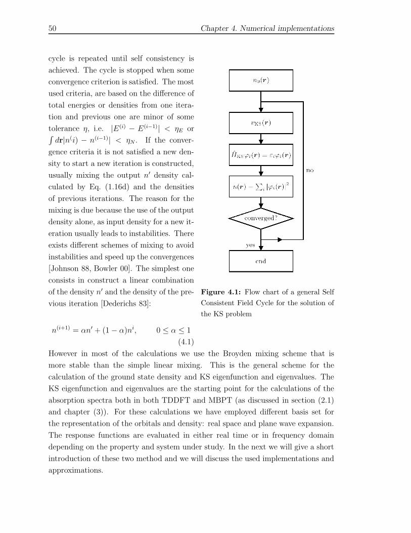
50 Chapter 4. Numerical implementations
Figure 4.1: Flow chart of a general Self
Consistent Field Cycle for the solution of
the KS problem
cycle is repeated until self consistency is
achieved. The cycle is stopped when some
convergence criterion is satisfied. The most
used criteria, are based on the difference of
total energies or densities from one itera-
tion and previous one are minor of some
tolerance η, i.e. |E(i) − E(i−1)| < ηE or∫
dr|n(i) − n(i−1)| < ηN . If the conver-
gence criteria it is not satisfied a new den-
sity to start a new iteration is constructed,
usually mixing the output n′ density cal-
culated by Eq. (1.16d) and the densities
of previous iterations. The reason for the
mixing is due because the use of the output
density alone, as input density for a new it-
eration usually leads to instabilities. There
exists different schemes of mixing to avoid
instabilities and speed up the convergences
[Johnson 88, Bowler 00]. The simplest one
consists in construct a linear combination
of the density n′ and the density of the pre-
vious iteration [Dederichs 83]:
n(i+1) = αn′ + (1 − α)ni, 0 ≤ α ≤ 1
(4.1)
However in most of the calculations we use the Broyden mixing scheme that is
more stable than the simple linear mixing. This is the general scheme for the
calculation of the ground state density and KS eigenfunction and eigenvalues. The
KS eigenfunction and eigenvalues are the starting point for the calculations of the
absorption spectra both in both TDDFT and MBPT (as discussed in section (2.1)
and chapter (3)). For these calculations we have employed different basis set for
the representation of the orbitals and density: real space and plane wave expansion.
The response functions are evaluated in either real time or in frequency domain
depending on the property and system under study. In the next we will give a short
introduction of these two method and we will discuss the used implementations and
approximations.

4.1 Real Space - Real Time representation: the OCTOPUS project 51
4.1 Real Space - Real Time representation: the
OCTOPUS project
The results reported in sections (6.1) and (6.2) on the optical properties of biolog-
ical systems have been carried out by means of TDDFT, where the excited states
have been calculated by direct evolution of the Time Dependent Kohn-Sham Equa-
tion as explained in section (2.2.2). For these calculations we have used the code
OCTOPUS. Here we examine some details of the implementation for such calculations
and we refer the reader to the paper[Marques 03a], to the Phd thesis of Alberto
Castro [Castro 04a]2 and to the code’s web site3 for a complete description of the
potentiality of this code, as well as for a tutorial and works done with this scheme.
4.1.1 The Grid
In a real space representation, a function φ is represented by its values set φj = φ(rj),
where rj is a set of points in a given simulation box. We have used an uniform
mesh, i.e. the points are equally spaced. The choice of having an uniform grid it
is not the most performing discretization, but it turns to be simple and intuitive.
However the present implementation allows for adaptive grids that are important
for some application where very different localization regions are present in the
simulation box. The simulation region can have different shapes, as sphere, cylinder
or parallelepiped. For our calculations we tested different shapes and finally we have
choose a grid made of overlapping spheres centered around the nuclei with a radius of
4 A, in this way we get a compromise between computational efficiency and precision
in the calculation. The radius of the sphere have to be carefully checked because
the wave-functions turns to be sensitive to the boundaries. A great advantage to
work with real space grid, besides easiness for parallelization in domains, is that
the potential operator is diagonal. To calculate the kinetic term, the Laplacian is
discretized and one needs the value of the wave function in the neighboring points:
∇2φ(ri) ≈∑
j∈Ki
cjφ(rj) (4.2)
where Ki is a set of neighboring point around ri and cj are real numbers defined
to approximate the Laplacian [Fornberg 94]. The lowest order rule to evaluate the
2 avalaible at http://dipc.ehu.es/arubio/docs/pdfs/a castro thesis.pdf3 http://www.tddft.org/programs/octopus
52 Chapter 4. Numerical implementations
Laplacian operator is in one dimension the three point rule that reads:
d2
dr2φ(r)
∣
∣
∣
ri' 1
4[φ(ri−1) − φ(ri) + φ(ri+1)] (4.3)
In our calculations we have used a higher order 9-point rule that allows to use a
larger mesh spacing4. An important detail is the evaluation of the Hartree term
Eq. (1.14). This term it is not efficiently evaluated performing a direct integration,
and it is obtained solving the Poisson equation:
∇2vH(r) = −4πn(r) (4.4)
This equation is solved in reciprocal space by performing a Fast Fourier Transform.
A particular attention have to be paid to completely cancel the spurious cell-cell
interaction when Eq. (4.4) is treated in Fourier space (see next chapter). This prob-
lem is solved imposing a cutoff to the Coulomb potential, and will be extensively
discussed in the next chapter. The parameters that controls the accuracy of the
calculation are the mesh spacing h and the kinetic energy discretization order. Un-
fortunately we have to mention that the real space implementation as such is not
variational, i.e. we can find a total energy lower than the true energy and reducing
the grid spacing the total energy can increase. Anyway for practical implementation
this is not a problem as the convergence with respect h can be easily checked.
4.1.2 The Time Evolution
In order to calculate the absorption spectra as described in section (2.2.2) the time
dependent Kohn-Sham equations (2.2) has to be solved. To propagate the electronic
wave-function in real time, we use a scheme designed to enforce time-reversal sym-
metry as implemented in OCTOPUS, i.e. we assume that the wave-function forward
propagated from, t to t+ ∆t/2 must be equal to the function backward propagated
from t + ∆t to t+ ∆t/2, i.e.:
e−iH(t)∆t2 φ(t) = eiH(t+∆t)∆t
2 φ(t+ ∆t) (4.5)
Such assumption yields:
φ(t+ ∆t) = e−iH(t+∆t)∆t2 e−iH(t)∆t
2 φ(t) (4.6)
4 For a general routine to generate the discretization of the kinetic energy operator see the
tutorial page of the OCTOPUS code http://www.tddft.org/programs/octopus and ref.[Beck 00,
Marques 03a]
4.2 Plane waves 53
We start by estimating φ(t + ∆t) ∼ e−iH(t)∆tφ(t) by expanding the exponential to
fourth order in ∆t.
e−iH∆t '4∑
n=0
(−i∆t)nn!
Hn (4.7)
Then this estimation is used to obtain an approximation for H(t+∆t), and finally the
expression(4.6) is computed again expanding the exponential to the fourth order.
We used a uniform grid-spacing of 0.23 A and a time-step of 0.0025 ~/eV. These
parameters ensure the stability of the time-dependent propagation and yield spectra
(Eq. 2.14) with a resolution better than 0.1 eV.
4.2 Plane waves
To calculate electronic properties of solids, a plane-wave expansion of the Kohn-
Sham wave functions turns to be very useful, because the periodicity of the system
is automatically taken into account working only with primitive cells to calculate
bulk properties. In such representation a Bloch wave function in periodic boundary
conditions is given by:
φnk(r) =1√Ωeik·r
∑
G
cnk(G)eiG·r = eik·runk(r). (4.8)
where unk(r) is a periodic function. The system is represented in a supercell of
volume Ω, the atoms are placed inside the supercell and translated according to
the symmetries properties of the system by the lattice vector Ri. The vectors k lie
within the first Brillouin zone (BZ) and G are the reciprocal lattice vectors. Other
great advantages of using the plane-wave expansion are:
• The translational symmetry of the potentials involved in the calculation is nat-
urally accounted in reciprocal space, and most expressions of the Hamiltonian
(1.16b) are analytic. The Kohn-Sham equation (1.16a) in this basis set reads:
∑
G′
hG,G′(k)cnk(G′) = εnkcnk(G), (4.9)
where the Hamiltonian matrix elements are:
hG,G′(k) =1
2|k+G|2δG,G′ +ν(k+G,k+G′)+vH [n](G−G′)+vxc[n](G−G′).
(4.10)
54 Chapter 4. Numerical implementations
In this representation the kinetic term is diagonal, and the Hartree term is
easily obtained as:
vH [n](G) = 4πn(G)
G2(4.11)
Note that the external potential depends on both G and G′ when non-local
norm-conserving pseudopotentials are used.
• There exists very efficient algorithms like FFTW[Frigo 98] that allow us to
calculate the Fourier transform very efficiently. Moreover there exists very
efficient pre-conditioning algorithms to speed up the SCF convergence.
• the expansion in plane waves is exact, since they form a complete set, and it is
only limited in practice by one parameter, namely, the maximum value of the
momentum, that determines the size of the chosen set. The usual criterion to
truncate the expansion is given by the convergence of the total energy. This
convergence can be achieved increasing the cutoff energy Ecutoff :
1
2|k + G|2 ≤ Ecutoff (4.12)
The number of plane wave involved in the calculation NPW scales as NPW ∝Ω(Ecutoff )
32 .
Although localized basis set are smaller for systems where localized electronic wave
functions are involved in the chemical binding, for instance for atoms, molecules
and clusters, plane-wave can be also be used in the supercell approach [Cohen 82,
Cohen 94, Pickett 89, Payne 92]. In the supercell approximation the physical system
is treated as a fully 3D periodic system, but a new unit cell (the supercell) is built
in such a way that some extra empty space separates the periodic replica along
the directions in which the system is to be considered as finite. This method make
possible to retain all the advantages of plane wave expansion mentioned above.
However, for finite system, a large number of plane waves is needed because the
density in concentrated in a small part of the total volume of the supercell. Moreover
the valence wave-functions of the atoms oscillates strongly in the neighbor of the
atomic core, due to the orthogonalization to the inner electronic wave function. For
this reason the use of pseudopotentials, apart the advantage to manage less electrons,
has the further advantage to reduce the energy cutoff. Yet the use of a supercell
to simulate objects that are not infinite and periodic in all the directions, leads to
artifacts, even if a very large portion of vacuum is interposed between the replica of

4.3 Technical details and implementations in the code SELF 55
the system in the non-periodic dimensions. In fact, the straightforward application
of the supercell method generates in any case fake images of the original system,
that can mutually interact in several ways, affecting the results of the simulation.
This problem is inherent not only to application of plane waves in supercell schemes,
but also to other methods where supercell approach is underlying the solution of
the many-body electronic problem as quantum-Montecarlo. In order to solve this
problem we have developed a cutoff Coulomb potential. The description and the
performance of such modified potential is the topic of the next chapter, as well as the
convergence problems with respect the empty space needed in the supercell approach
for the optical and electronic properties of non 3D systems. In the work exposed
in chapter (7), where we have studied optical properties of finite and infinite chains
of atoms, we have chosen to work in the supercell approach, and the new cutoff
potential has been used in all the calculations. The ground state KS wave-functions
and eigenvalues have been calculated using the plane-wave code ABINIT [Gonze 05]5.
For the optical properties both in TDDFT and MBPT framework we have used the
code SELF6. This is also a plane wave code, developed in our group, and all the
quantities are expressed in reciprocal space, details on how the main quantities have
been calculated with this code will be given in the next section.
4.3 Technical details and implementations in the
code SELF
The GW calculation
As discussed in section (3.3) in the GW approximation, the non-local energy-dependent
electronic self-energy Σ plays a role similar to that of the exchange-correlation po-
tential of DFT. Σ is approximated by the convolution of the one electron Green’s
function and the dynamically screened Coulomb interaction W Eq. (3.21c). The
quasiparticle energies have been calculated at the first order of perturbation theory
in Σ−Vxc.[Hybertsen 85, Godby 88] as in Eq. (3.24). We first divide the Self-energy
in an exchange Σx and a correlation Σc parts
〈φDFTj |Σ|φDFTi 〉 = 〈φDFTj |Σx|φDFTi 〉 + 〈φDFTj |Σc|φDFTi 〉. (4.13)
5 http://www.abinit.org6 http://people.roma2.infn.it/∼marini/self
56 Chapter 4. Numerical implementations
where :
Σx(r, r′) =iv(r, r′)G0(r, r′, t+ 0−) (4.14a)
Σc(r, r′, t) =iW (r, r′, t)G0(r, r′, t) (4.14b)
Here v is the bare coulomb potential and W it is not the full screening but only its
frequency dependent part:
W (r, r′, t) =
∫
dr1v(r, r1)ε−1(r′, r1, t) (4.15)
and ε−1(r, r′, t) =∫
dr1v(r, r1)χ(r, r′, t) and χ is given by Eq. (5.30). We get the
following representation for the Self energy in a plane-waves basis set:
〈nk|Σx(r1, r2)|n′k′〉 = −∑
n1
∫
Bz
d3q
(2π)3
∑
G
v(q + G)×
× ρnn1(q,G)ρ?n′n1(q,G)fn1k1
(4.16)
and
〈nk|Σc(r1, r2, ω)|n′k′〉 =1
2
∑
n1
∫
Bz
d3q
(2π)3
∑
GG′
v(q + G′)
× ρnn1(q,G)ρ?n′n1(q,G′)
∫
dω′
2πε−1GG′(q, ω
′)
×[ fn1(k−q)
ω − ω′ − εLDAn1(k−q) − iδ+
1 − fn1(k−q)
ω − ω′ − εLDAn1(k−q) + iδ
]
(4.17)
where ρnn1(q + G) = 〈nk|ei(q+G)·r1|n1k1〉. The integral in the frequency domain in
Eq. (4.17) has been analytically solved considering the dielectric matrix in the plas-
mon pole model [Godby 89]. This approximation to the inverse dielectric matrix is
based on the observation that in realistic calculations of response function Imε−1(ω)
is a peaked function in ω. Such defined peaks corresponds to plasmon excitations
of the system. With this in mind we can approximate the energy dependence of the
imaginary part of each element of ε−1 with a narrow Lorentzian peak. Using the
Kramers-Kroning relation the inverse dielectric matrix in reciprocal space is given
by:
ε−1G,G′(ω) = δG,G′ + ΩG,G′/(ω
2 − ω2G,G′) (4.18)
Note that here the energy ω is a complex variable. The position ωG,G′ and the
strength ΩG,G′ of the poles are obtained fitting a full calculation along the imagi-
nary energy axis. So a full calculation for only two frequencies (ω = 0 and ω = iE0)
4.3 Technical details and implementations in the code SELF 57
is needed in order to find the the poles and residuum for each component. We have
tested the validity of this approximation performing calculation of the gap either in
the case of an infinite polymer of polyacetylene or isolate molecule of C2H4 (a single
monomer of polyacetylene) calculating the Σc with a direct integration in the fre-
quency domain. Such calculations turns to be very cumbersome and the differences
with the results of the gap energy obtained with the plasmon-pole approximation
have been less then 5%. Thus, we have decided to use the plasmon-pole approxima-
tion for all the calculations presented in chapters (5) and (7).
The Bethe Salpeter equation
We have described in section (3.4) the structure of the Excitonic Hamiltonian, and
the different terms of each element of the excitonic matrix have been illustrated
in Eqs.(3.44,3.45,3.46). The basis set to describe the exciton state is composed by
product states of the occupied and unoccupied LDA single particle states and the
coupled electron-hole excited states Eq. (3.41), taking only the resonant term now
can be written in terms of electron and hole coordinates as:
ΨS(rh, re) =∑
v,c,k
A(vck)S φ∗
vk(rh)φck(re) (4.19)
where e stands for electron and h for hole. With these assumption, when only
the resonant part of the Hamiltonian is taken into account Eq. (3.40) reads:
(εQPck − εQPvk )AvckS +∑
vck,v′c′k′
Kvck,v′c′k′Av′c′k′
S = ESAvckS (4.20)
ES is the excitation energy of the state ΨS and K the interaction kernel that in-
cludes an unscreened exchange repulsive term 2KExch and a screened electron-hole
interaction Kdir (direct term). The factor two that multiplies the exchange part
enters for considering spin singlet excitations. In plane wave basis such terms for
the resonant part read:
2KExch,res
( vckv′c′k′)
=2
Ω
∑
G6=0
v(G)〈ck|eiG·r|vk〉〈v′k′|e−iG′·r|c′k′〉 (4.21)
Kdir,res
( vckv′c′k′)
=1
Ω
∑
G,G′
v(q + G)ε−1GG′(q)〈ck|ei(q+G)·r|c′k′〉×
× 〈v′k′|e−i(q+G′)·r|vk〉δq.k−k′
(4.22)
58 Chapter 4. Numerical implementations
The screened potential has been treated in static RPA approximation (dynamical
effects in the screening have been neglected as it is usually done in present Bethe-
Salpeter calculations[Onida 02, Albrecht 98, Benedict 98, Rohlfing 98, Rohlfing 00]).
For bulk systems the off-diagonal blocks, of the excitonic matrix (3.43), the so-called
coupling terms Eq. (3.46) are found to be small and have nearly no effect on the ex-
citation energies [Albrecht 98, Rohlfing 98]. However, as we will see in chapter (7),
for finite systems they can play a role. For this reason we have implemented the
coupling terms in the code SELF. The unscreened exchange term is from Eq. (3.46):
2KExch,cpl
( vckc′v′k′)
=2
Ω
∑
G6=0
v(G)〈ck|eiG·r|vk〉〈c′k′|e−iG′·r|v′k′〉 (4.23)
and the direct screened coulomb term:
Kdir,cpl
( vckc′v′k′)
=1
Ω
∑
G,G′
v(q + G)ε−1GG′(q)〈ck|ei(q+G)·r|v′k′〉×
× 〈c′k′|e−i(q+G′)·r|vk〉δq.k−k′
(4.24)
Note that when the coupling terms are taken into account, the dimension of excitonic
matrix to diagonalize is four times bigger than the only-resonant case, with the
additional complication that the matrix is no more Hermitian.
The fxc kernel from the Bethe Salpeter equation
In section (3.5) we have derived an expression for a non-local and energy dependent
kernel imposing that TDDFT reproduce the perturbative expansion of the BS equa-
tion in terms of the screened coulomb potential. At first order the expression of fxc
is given in Eq. (3.54). A direct application of this expression leads to spurious oscil-
lations, and in many case it give rise to non-physical regions of negative absorption.
The reason of such oscillations is imputable to the diagonal part of the kernel of the
BS equation (Eq. 3.51). The diagonal part of the BS equation:
∆(q)K = WK,K(q) (4.25)
is responsible for the shifting of the spectra, and can be shown [Marini 03] that
it appears in fxc through a series expansion in ∆(q)K . Of course, a perturbative
treatment is meaningful only if ∆(q)K is small. This is not the case for the systems
that we have treated in chapter (7), where it is of the order of 1 eV. To overcome this
4.3 Technical details and implementations in the code SELF 59
issue we include the diagonal part of the kernel of the BS equation in the independent
quasiparticle response function P 0(q, ω), and the fxc will take into account all the
off-diagonal contribution. Explicitly we can rewrite the equation (3.50) as:
PBSK1,K2
(q, ω) = P 0K1,K2
(q, ω + ∆)− P 0K1,K3
(q, ω + ∆)WK3,K4(q)PBSK4,K2
(q, ω) (4.26)
where now
WK1,K2 =
0 K1 = K2
WK1,K2 otherwise(4.27)
and the corresponding expression for the f(1)xc will be now given by:
f (1)xc (q, ω) = [P 0(q, ω + ∆)]−1δP (1)(q, ω)[P 0(q, ω + ∆)]−1 (4.28)
where in the expression of δP (1) (Eq. (3.55)) the diagonal part of W has been
removed. With this trick the TDDFT calculations of the absorption spectra are
numerically stable. Moreover we have applied a fast procedure to calculate the kernel
at first order as indicated in Ref. [Marini 03]. Looking ad the analytic properties of
δP (1) Eq. (3.55), the contribution of degenerate non-interacting electron-hole states
in Eq. (3.34) are singled out and the expression for fxc reads:
f (1)xc (q, ω) =
2
Ω[P 0(q, ω + ∆)]−1
∑
K
[ R(q)K + R
(q)†
K
ω + ∆(q)K − E
(q)K + iη
+
Q(q)K
(ω + ∆(q)K − E
(q)K + iη)2
]
[P 0(q, ω + ∆)]−1
(4.29)
Here the sum runs over the independent electron-hole states and the residuum are
given by:
[R(q)K ]G1,G2 =
∑
K′,E(q)
K′ 6=E(q)
K′
Φ∗K(q,G1)WK,K′(q)ΦK′(q,G2)
E(q)K − E
′(q)K
for non degenerate states
[Q(q)K ]G1,G2 =
∑
K′,E(q)
K′ =E(q)
K′
Φ∗K(q,G1)WK,K′(q)ΦK′(q,G2) for degenerate states
(4.30)
Eq. (4.29) turns to be much faster to calculate than Eq. (3.55): it has the form
of a non-interacting polarization function with modified residuals that are evalu-
ated only once by a two matrix-vector multiplication. Looking at the expression

60 Chapter 4. Numerical implementations
(4.28) to obtain the many-body based fxc we can see that another complication
arise. Until now we have implicitly assumed that P 0 is an invertible matrix. Mearns
and Kohn [Mearns 87] showed that when the energy range taken into account is
above the first resonance, as in the case of the absorption spectra, non trivial van-
ishing eigenvalue occurs, and the inversion leads to numerical problems. We have
overcome this problem using the Singular Value Decomposition (SVD) [Press 92],
finding a window for the threshold that give stable solution for the spectra shown
in chapter (7).

5 An exact Coulomb cutoff
technique for supercell
calculations†
In section (4.2) we have described the main advantages of the use of plane-wave basis
set in the calculation of electronic and optical properties of infinite crystal solids.
However, mainly in the last decade, increasing interest has been developed in systems
at the nano-scale, like tubes, wires, quantum-dots, biomolecules, etc., whose phys-
ical dimensionality is, for all practical purposes, less than three[Nalwa 05]. These
systems are still 3-dimensional (3D), but their quantum properties are those of a
confined system in one or more directions, and those of a periodic extended sys-
tem in the remaining directions. Other classes of systems with the same kind of
reduced periodicity are the classes of the polymers, and of the solids with defects.
Throughout this chapter we call nD-periodic a 3D object, that can be considered
infinite and periodic in n dimensions, being finite in the remaining 3 − n dimen-
sions. . It is well known that the response function of an overall neutral solid of
molecules is not equal, in general, to the response of the isolated molecule, and con-
verges very slowly to it, when the amount of vacuum in the supercell is progressively
increased.[Onida 02, Sottile 05] For instance, the presence of higher order multipoles
can make undesired images interact via the long range part of the Coulomb poten-
tial. In the dynamic regime, multipoles are always generated by the oscillations of
the charge density even in systems whose unit cell does not carry any multipole in
its ground state. This is the case, for example, when we investigate the response
of a system in presence of an external oscillating electric field. Things go worse
when the unit cell carries a net charge, since the total charge of the infinite system
represented by the supercell is actually infinite, while the charges at the surfaces of
† This section is largely an adaptation of the article: C.A. Rozzi, D. Varsano, A. Marini, A.
Rubio and E.K.U. Gross: An exact Coulomb cutoff technique for supercell calculations
accepted in Phys. Rev. B (2006). As such, the reported work includes collaboration of the rest
of the authors of the article. The paper can be download from cond-mat 0601031
61
62 Chapter 5. An exact Coulomb cutoff technique for supercell calculations
a finite, though very large, system always generate a finite polarization field. This
situation is usually normalized in the calculation by the introduction of a suitable
compensative positive background charge. Another common situation in which the
electrostatics is known to modify the ground state properties of the system occurs
when a layered system is studied, and an infinite array of planes is considered instead
of a single slab, being in fact equivalent to an effective chain of capacitors[Wood 04].
These issues become particularly evident in all the approaches that imply the cal-
culation of non-local operators or response functions, because, in these cases, two
supercells may effectively interact even if their charge densities do not overlap at
all. This is the case, for example, of the many-body perturbation theory calcula-
tions (MBPT), and, in particular, of the self-energy calculations at the GW level.
However we are usually still interested in the dispersion relations of the elementary
excitations of the system along its periodic directions, and those are ideally dealt
with using a plane waves approach. Therefore, the ideal path to keep the advantages
of the supercell formulation in plane waves on the use of FFT to solve the Poisson
equation, even in real space implementation, and to gain a description of systems
with reduced periodicity free of spurious effects is to develop a technique to cut the
Coulomb interaction off out of a desired region. FFT turns to be very fast and this
approach is worth compared to other multipole expansion that allow to treat the
proper boundary conditions for the Poisson equation in real space without resorting
to supercell approach. This problem is not new and has been addressed now for
a very long time and in different fields and several different approaches have been
proposed in the past to solve it. The aim of the present work is to focus on the
widely used supercell schemes to show how the image interaction influences both
the electronic ground state properties and the dynamical screening in the excited
state of 0D-, 1D-, 2D-periodic systems, and to propose an exact method to avoid
the undesired interaction of the replicas in the non-periodic directions. The chapter
is organized as follows: in section (5.1) we review more in detail the problem of the
solution of the Poisson equation in the plane wave method for solids, in section (5.2)
the new method is outlined, in section (5.3) the treatment of the singularities is ex-
plained, in section (5.4) some applications of the proposed technique are discussed.

5.1 The 3D-periodic case 63
5.1 The 3D-periodic case
The main problem of electrostatics we are facing here can be reduced to the problem
of finding solutions to the Poisson equation for a given charge distribution n(r), and
given boundary conditions
∇2V (r) = −4πn(r). (5.1)
In a finite system the potential is usually required to be zero at infinity. In a
periodic system this condition is meaningless, since the system itself extends to
infinity. Nevertheless the general solution of Eq. (5.1) in both cases is known in the
form of the convolution
V (r) =
∫∫∫
space
n(r′)
|r − r′|d3r′, (5.2)
that it is referred from now on as the Hartree potential. It might seem that the
most immediate way to build the solution potential for a given charge distribution
is to compute the integral in real space, but problems immediately arise for infinite
systems. In fact, the density can be reduced to an infinite sum over delta charge dis-
tributions qδ(r−r′), and the integral in Eq. (5.2) becomes an infinite sum as well, but
this sum is in general only conditionally, and not absolutely convergent.[Makov 95]
V (r) =∑
n
q
|r − Ln|, (5.3)
This sum gives a potential that is determined up to a constant for a neutral cell with
zero dipole moment, while the corresponding sum for the electric field is absolutely
convergent. A neutral cell with a non null dipole moment, on the opposite, gives
a divergent potential, and an electric field that is determined up to an unknown
constant electric field (the sum for the electric field is conditionally convergent in this
case). Even if, in principle, the surface terms have to be always taken into account,
in practice they are only relevant when we want to calculate energy differences
between states with different total charge. These terms can be neglected in the
case of a neutral cell whose lowest nonzero multipole is quadrupole[DeLeeuw 80].
As in the present work we are interested in macroscopic properties of the periodic
system, those surface effects are never considered in the discussion that follows.
However this sample-shape effects play an important role for the analysis of different
spectroscopies as , for example, infrared and nuclear-magnetic resonance. A major
source of computational problems is the fact that the sum in Eq. (5.3) is very
slowly converging when it is summed in real space, and this fact has historically

64 Chapter 5. An exact Coulomb cutoff technique for supercell calculations
motivated the need for reciprocal space methods to calculate it. It was Ewald who
first discovered that, by means of an integral transform, the sum can be split in two
terms, and that if one is summed in real, while the other in reciprocal space, both of
them are rapidly converging.[Ewald 21] The point of splitting is determined by an
arbitrary parameter. Let us now focus on methods of calculating the sum in Eq. (5.3)
purely based on the reciprocal space. If we consider a periodic distribution of charges
with density n(r) such that n(r) = n(r + Ln), with Ln = nxLx, nyLy, nzLz, and
nx, ny, nz ∈ Z, it turns out that the reciprocal space expression for a potential like
V (r) =
∫∫∫
space
n(r′)v(|r − r′|)d3r′, (5.4)
in a 3D-periodic system, can be written as
V (Gn) = n(Gn)v(Gn), (5.5)
where we have used the convolution theorem to transform the real space convolution
of the density and the Coulomb potential into the product of their reciprocal space
counterparts. Here Gn = nxGx, nyGy, nzGz are the multiples of the primitive
reciprocal space vectors 2πLn
, and v(Gn) is the Fourier transform of the long range
interaction v(r), evaluated at the point Gn. For the Coulomb potential it is
v(Gn) =4π
G2n
. (5.6)
Fourier transforming expression (5.5) back into real space we have, for a unit cell of
volume Ω,
V (r) =4π
Ω
∑
n6=0
n(Gn)
G2n
exp(iGn · r). (5.7)
At the singular point Gx = Gy = Gz = 0 the potential V is undefined, but, since
the value at G = 0 corresponds to the average value of V in real space, it can be
chosen to be any number, corresponding to the arbitrariness in the choice of the
static gauge (a constant) for the potential. Observe that the same expression can
be adopted in the case of a charged unit cell, but this time, the arbitrary choice of
v(G) in G = 0 corresponds to the use of a uniform background neutralizing charge.
5.2 System with reduced periodicity
It has been shown[Spohr 94] that the slab capacitance effect mentioned in the in-
troduction actually is a problem that cannot be solved by just adding more vac-
5.2 System with reduced periodicity 65
uum to the supercell. This has initially led to the development of corrections
to Ewald’s original method[Yeh 99], and then to rigorous extensions in 2D and
1D.[Martyna 99, Brodka 03] The basic idea is to restrict the sum in reciprocal space
to the reciprocal vectors that actually correspond to the periodic directions of the
system. These approach are in general of order O(N 2)[Heyes 77, Grzybowski 00],
but they have been recently refined to order O(N lnN).[Minary 02, Minary 04]
Another class of techniques, developed so far for finite systems, is based on the
expansion of the interaction into a series of multipoles (fast multipole method)
[Greengard 88, Castro 03, Kudin 04]. With this technique it is possible to evaluate
effective boundary conditions for the Poisson’s equations at the cell’s boundary, so
that the use of a supercell is not required at all, making it computationally very
efficient for finite[Greengard 88, Castro 03] and extended systems[Kudin 04]. Dif-
ferently from what happens for the Ewald sum, the method that we propose to
evaluate the sum n Eq. (5.3), entirely relies on the Fourier space and amounts to
screening the unit cell from the undesired effect of (some of) its periodic images.
The basic expression is Eq. (5.5), whose accuracy is only limited by the maximum
value GN of the reciprocal space vectors in the sum. Since there is no splitting
between real and reciprocal space, no convergence parameters are required. Our
goal is to transform the 3D-periodic Fourier representation of the Hartree potential
of Eq. (5.5) into the modified one
V (Gn) = n(Gn)v(Gn) (5.8)
such that all the interactions among the undesired periodic replica of the system
disappear. The present method is a generalization of the method proposed by Jarvis
et al.[Jarvis 97] for the case of a finite system. In order to build this representation,
we want to:
i. define a screening region D around each charge in the system, out of which
there is no Coulomb interaction
ii. calculate the Fourier transform of the desired effective interaction v(r) that
equals the Coulomb potential in D, and is 0 outside D:
V (r) =
1r
if r ∈ D0 if r /∈ D
. (5.9)
iii. Finally we must modify the density n(r) in such a way that the effective
density is still 3D-periodic, so that the convolution theorem can be still applied,

66 Chapter 5. An exact Coulomb cutoff technique for supercell calculations
but densities belonging to undesired images are not close enough to interact
through v(r).
The choice of the region D for step i) is suggested by symmetry considerations, and
it is a sphere (or radius R) for finite systems, an infinite cylinder (of radius R) for
1D-periodic systems, and an infinite slab (of thickness 2R) for 2D-periodic systems.
Step ii) means that we have to calculate the modified Fourier integral
V (G) =
∫∫∫
space
v(r)e−iG·rd3r =
∫∫∫
D
v(r)e−iG·rd3r. (5.10)
Still we have to avoid that two neighboring images interact by taking them far away
enough from each other. Then step iii) means that we have to build a suitable
supercell, and re-define the density in it. Let us examine first step ii), i.e. the cutoff
Coulomb interaction in reciprocal space. We know the expression of the potential
when it is cutoff in a sphere.[Jarvis 97] It is
v0D(G) =4π
G2
[
1 − cos(GR)]
. (5.11)
The limit R → ∞ converges in a oscillatory form to the bare Coulomb term in the
sense of a distribution, while, since limG→0 = 2πR2, there is no particular difficulty in
the origin. This scheme has been successfully used in many applications[Makov 95,
Jarvis 97, Castro 03, Marques 03a, Onida 95]. The 1D-periodic case applies to sys-
tems with infinite extent in the x direction, and finite in the y and z directions.
The effective Coulomb interaction is then defined in real space to be 0 out of a
cylinder of radius R having its axis parallel to the x direction. By performing the
Fourier transformation we get the following exact expression for the cutoff coulomb
potential in cylindrical coordinates:[I.S. Gradshteyn 80]
v1D(Gx, G⊥) =4π
G2
[
1 +G⊥RJ1(G⊥R)K0(|Gx|R) − |Gx|RJ0(G⊥R)K1(|Gx|R)
]
,
(5.12)
where J and K are the ordinary and modified cylindrical Bessel functions, and G⊥ =√
G2y +G2
z. It is easy to realize that, since the K functions damp the oscillations of
the J functions very quickly, for all practical purposes this cutoff function only acts
on the very first smaller values of G, while the unscreened 4πG2 behavior is almost
unchanged for the larger values. Unfortunately, while the Jn(ξ) functions have a
constant value for ξ = 0, and the whole cutoff is well defined for G⊥ = 0, the K0(ξ)
5.2 System with reduced periodicity 67
function diverges logarithmically for ξ → 0. Since, on the other hand, K1(ξ) ≈ ξ−1
for small ξ,
V 1D(Gx, G⊥) ∼ − log(GxR) for G⊥ > 0, Gx → 0+. (5.13)
This means that the limit limG→0+ v(G) does not exist for this cutoff function, and
the whole Gx = 0 plane is ill-defined. We will come back to the treatment of the
singularities in the next section. We notice that this logarithmic divergence is the
common dependence one would get for the electrostatic potential of a uniformed
charged 1D wire[Jackson 75], it is expected that bringing charge neutrality in place
would cancel this divergence (see below). The 2D-periodic case, with finite extent in
the z direction, is calculated in a similar manner. The effective Coulomb interaction
is defined in real space to be 0 out of a slab of thickness 2R symmetric with respect
to the xy plane. In Cartesian coordinates we get
v2D(G‖, Gz) =4π
G2
[
1 + e−G‖R|Gz|G‖
sin(|Gz|R) − e−G‖R cos(|Gz|R)
]
, (5.14)
where G‖ =√
G2x +G2
y. In the limit R → ∞ the unscreened potential 4πG2 is recov-
ered. Similarly to the case of 1D, the limit G → 0 does not exist, since for Gz = 0,
the cutoff has a finite value, while it diverges in the limit G‖ → 0
V 2D(G‖, Gz) ∼1
G2‖
for G‖ > 0, Gz → 0+. (5.15)
So far we haven’t committed to a precise value of the cutoff length R. This value has
to be chosen, for each dimensionality, in such a way that it avoids the interaction
of any two neighbor images of the unit cell in the non-periodic dimension. In order
to fix the values of R we must choose the size of the supercell. This leads us to
the step 3) of our procedure. We recall that even once the long range interaction is
cutoff out of some region around each component of the system, this is not sufficient
yet to avoid the interaction among undesired images. The charge density has to
be modified, or, equivalently, the supercell has to be built in such a way that two
neighboring densities along every non periodic direction do not interact via the
cutoff interaction. It is easy to see how this could happen in the simple case of a
2D square cell of length L: if both r and r′ belongs to the cell, then r, r′ ≤ L, and
|r − r′| ≤√
2L (see the schematic drawing in Fig. 5.1). If a supercell is built that
is smaller than (1 +√
2)L, there could be residual interaction, and the cutoff would
no longer lead to the exact removal of the undesired interactions. Let us call A0 the

68 Chapter 5. An exact Coulomb cutoff technique for supercell calculations
!!!!!!!!!!!!!!!!!!!!!!!!!!!!!!!!!!!!!!!!!!!!!!!!!!!!!!""""""""""""""""""""""""""""""""""""""""""""""""""""""
#############################################$$$$$$$$$$$$$$$$$$$$$$$$$$$$$$$$$$$$$$$$$$$$$
%%%%%%%%%%%%%%%%%%%%%%%%%%%%%%%%%%%%%%%%%%%%%%%%%%%%%%&&&&&&&&&&&&&&&&&&&&&&&&&&&&&&&&&&&&&&&&&&&&&
''''''''''''''''''''''''''''''''''''''''''''''''''''''(((((((((((((((((((((((((((((((((((((((((((((
))))))))))))))))))))))))))))))))))))))))))))))))))))))******************************************************
(1 +√
(2))L
L
Figure 5.1: Schematic description for the supercell construction in a 2D system. The
upper scheme corresponds to the 2D-periodic case (i.e.a 2D crystal). The middle sketch
corresponds to a 0D-periodic system, and the bottom one to a 1D-periodic. In the 0D-
periodic case the system in different cells do not interact while in the 1D-periodic the chains
do not interact, but within each chain the interaction of all of its elements is permitted..
unit cell of the system we are working on, and A = Ai, i = −∞, · · · ,∞ the set
of all the cells in the system. If the system is nD-periodic this set only includes the
periodic images of A0 in the n periodic directions. Let us call B the set of all the
non-physical images of the system, i.e. those in the non-periodic directions. Then
A∪B = R3. Obviously, if the system is 3D-periodic A = R
3, and B ≡ ∅. In general
we want to allow the interaction of the electrons in A0 with the electrons in all the
cells Ai ∈ A, but not with those Bi ∈ B. To obtain this we define the supercell

5.3 Cancellation of singularities 69
C0 ⊇ A0 such that, ∀i
if r ∈ A0, and r′ ∈ Ai then |r − r′| ∈ C0
if r ∈ A0, and r′ ∈ Bi then |r − r′| /∈ C0
(5.16)
(see Fig. 5.1 for a simplified 2D sketch). The new density n(r) is such that
if r ∈ A0 then n(r) = n(r),
if r ∈ C0, and r /∈ A0 then n(r) = 0.(5.17)
The size of the super-cell in the non-periodic directions depends on the periodic
dimensionality of the system. In order to completely avoid any interaction, even in
the case the density of the system is not zero at the cell border, it has to be
LC = (1 +√
3)LA for finite
LC = (1 +√
2)LA for 1D-periodic
LC = 2LA for 2D-periodic
(5.18)
Actually, since the required super-cell is quite large, a compromise between speed
and accuracy can be achieved in the computation, using parallelepiped super-cell
with LC = 2LA for all the cases. This approximation rests on the fact that, usually,
the charge density is contained in a region smaller than the cell in the non-periodic
directions, so that the spurious interactions are, in fact, avoided, even with a smaller
cell. Therefore, on the basis of this approximation, we can choose the value of the
cutoff length R always as half the smallest primitive vector in the non-periodic
dimension.
5.3 Cancellation of singularities
The main point in the procedure of eliminating the divergences in all the cases of
interest is to observe that our final goal is usually not to obtain the expression
of the Hartree potential alone, because all the physical quantities depend on the
total potential, i.e. on the sum of the electronic and the ionic potential. When
this sum is considered we can exploit the fact that each potential is defined up to
an arbitrary additive constant, and choose the constants consistently for the two
potentials. Since we know in advance that the sum must be finite, we can include
into this constants all the infinities, provided we find a method to separate them
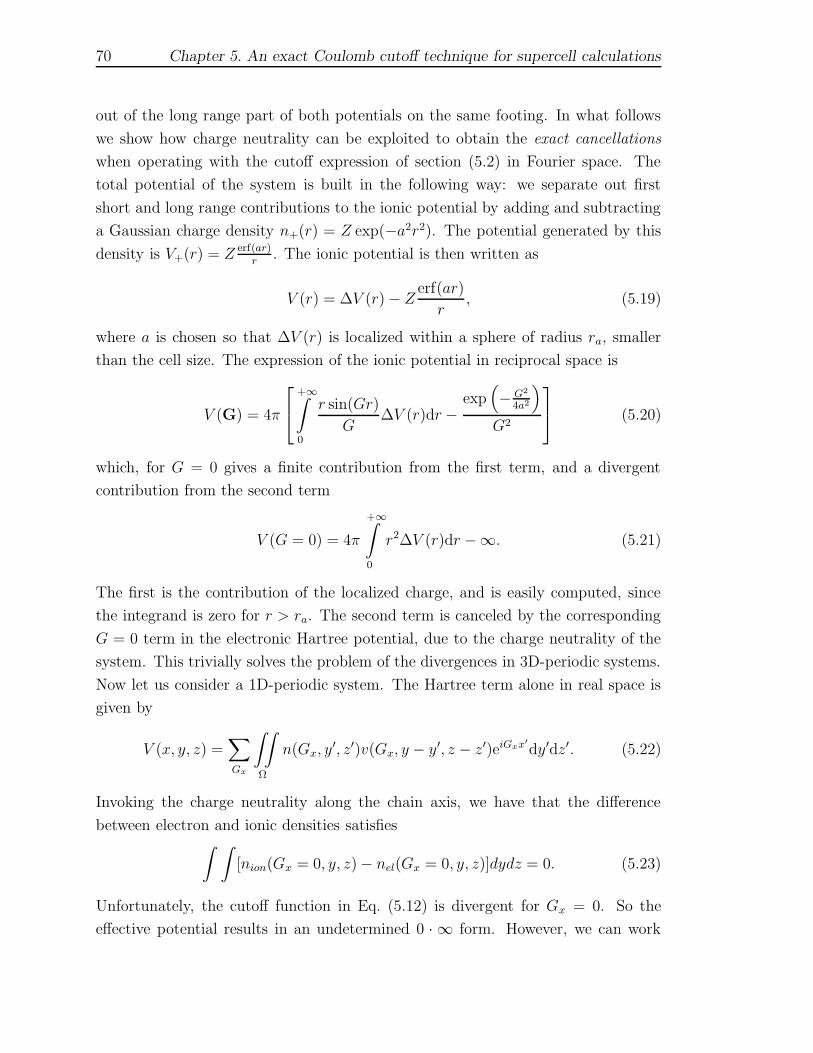
70 Chapter 5. An exact Coulomb cutoff technique for supercell calculations
out of the long range part of both potentials on the same footing. In what follows
we show how charge neutrality can be exploited to obtain the exact cancellations
when operating with the cutoff expression of section (5.2) in Fourier space. The
total potential of the system is built in the following way: we separate out first
short and long range contributions to the ionic potential by adding and subtracting
a Gaussian charge density n+(r) = Z exp(−a2r2). The potential generated by this
density is V+(r) = Z erf(ar)r
. The ionic potential is then written as
V (r) = ∆V (r) − Zerf(ar)
r, (5.19)
where a is chosen so that ∆V (r) is localized within a sphere of radius ra, smaller
than the cell size. The expression of the ionic potential in reciprocal space is
V (G) = 4π
+∞∫
0
r sin(Gr)
G∆V (r)dr −
exp(
− G2
4a2
)
G2
(5.20)
which, for G = 0 gives a finite contribution from the first term, and a divergent
contribution from the second term
V (G = 0) = 4π
+∞∫
0
r2∆V (r)dr −∞. (5.21)
The first is the contribution of the localized charge, and is easily computed, since
the integrand is zero for r > ra. The second term is canceled by the corresponding
G = 0 term in the electronic Hartree potential, due to the charge neutrality of the
system. This trivially solves the problem of the divergences in 3D-periodic systems.
Now let us consider a 1D-periodic system. The Hartree term alone in real space is
given by
V (x, y, z) =∑
Gx
∫∫
Ω
n(Gx, y′, z′)v(Gx, y − y′, z − z′)eiGxx′dy′dz′. (5.22)
Invoking the charge neutrality along the chain axis, we have that the difference
between electron and ionic densities satisfies∫ ∫
[nion(Gx = 0, y, z) − nel(Gx = 0, y, z)]dydz = 0. (5.23)
Unfortunately, the cutoff function in Eq. (5.12) is divergent for Gx = 0. So the
effective potential results in an undetermined 0 · ∞ form. However, we can work

5.3 Cancellation of singularities 71
out an analytical expression for it based on conditional convergence of the coulomb
potential in periodic system, by defining a finite cylindrical cutoff and then make
the limit of the size of the cylinder to infinity. In this way, as first step, we get a
new cutoff interaction in a finite cylinder of radius R, and length h, assuming that h
is much larger than the cell size in the periodic direction. In this case the modified
finite cutoff potential includes a term:
V 1D(Gx = 0, r) ∝ log(h +
√h2 + r2
r
)
(5.24)
which, in turn gives, for the particular plane Gx = 0,
v1D(Gx = 0, G⊥) ≈ −4π
R∫
0
rJ0(G⊥r) log(r)dr + 4πR log(2h)J1(G⊥R)
G⊥. (5.25)
The effective potential is now split into two terms, but only the second one depends
on h. The second step is achieved by going to the limit h → +∞, to obtain the
exact infinite cutoff. By calculating this limit, we notice that only the second term
in Eq. (5.25) diverges. This term is the one that can be dropped due to charge
neutrality (in fact it has the same form for the ionic and electronic charge densi-
ties). Thus, for the cancellation to be effective in a practical implementation we
have to treat on the same way both the ionic and Hartree Coulomb contributions.
Of course the first term has always to be taken into account, affecting both the long
and the short range part of the cutoff potentials. Following this procedure, we are
able to get a considerable computational advantage, compared to the method orig-
inally proposed by Spataru et al [Spataru 04a], since our cutoff is just an analytical
function of the reciprocal space coordinates, and the evaluation of an integral for
every value of Gx, G⊥ is not needed. The cutoff proposed in Ref.[Spataru 04a] is
actually a particular case of our cutoff, obtained by using the finite cylinder for all
the components of the G vectors: in this case the quadrature in Eq. (5.25) has to
be evaluated for each Gx,Gy and Gz, and a convergence study in h is mandatory.
In the 1D-periodic case, the G = 0 value is now well defined, and it turns out to be
limG⊥→0 v(Gx, G⊥)
v1D(Gx = 0, G⊥ = 0) = −πR2(2 log(R) − 1). (5.26)
The analogous result for the 2D-periodic cutoff is obtained by imposing finite cutoff
sizes hx = αhy = h (much larger than the cell size), in the periodic directions x and
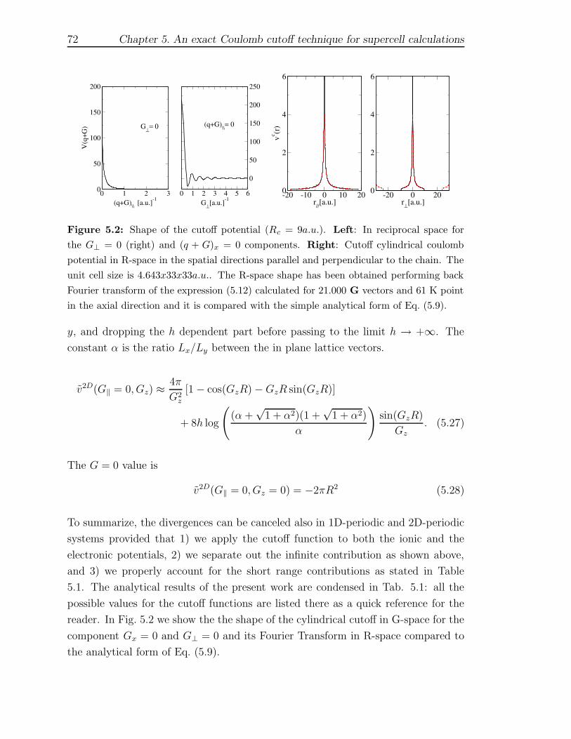
72 Chapter 5. An exact Coulomb cutoff technique for supercell calculations
0 1 2 3(q+G)\\ [a.u.]-1
0
50
100
150
200V
(q+G
)
0 1 2 3 4 5 6G⊥[a.u.]-1
0
50
100
150
200
250
G⊥= 0 (q+G)\\= 0
-20 -10 0 10 20r//[a.u.]
0
2
4
6
vc (r)
-20 0 20r⊥[a.u.]
0
2
4
6
Figure 5.2: Shape of the cutoff potential (Rc = 9a.u.). Left: In reciprocal space for
the G⊥ = 0 (right) and (q + G)x = 0 components. Right: Cutoff cylindrical coulomb
potential in R-space in the spatial directions parallel and perpendicular to the chain. The
unit cell size is 4.643x33x33a.u.. The R-space shape has been obtained performing back
Fourier transform of the expression (5.12) calculated for 21.000 G vectors and 61 K point
in the axial direction and it is compared with the simple analytical form of Eq. (5.9).
y, and dropping the h dependent part before passing to the limit h → +∞. The
constant α is the ratio Lx/Ly between the in plane lattice vectors.
v2D(G‖ = 0, Gz) ≈4π
G2z
[1 − cos(GzR) −GzR sin(GzR)]
+ 8h log
(
(α +√
1 + α2)(1 +√
1 + α2)
α
)
sin(GzR)
Gz. (5.27)
The G = 0 value is
v2D(G‖ = 0, Gz = 0) = −2πR2 (5.28)
To summarize, the divergences can be canceled also in 1D-periodic and 2D-periodic
systems provided that 1) we apply the cutoff function to both the ionic and the
electronic potentials, 2) we separate out the infinite contribution as shown above,
and 3) we properly account for the short range contributions as stated in Table
5.1. The analytical results of the present work are condensed in Tab. 5.1: all the
possible values for the cutoff functions are listed there as a quick reference for the
reader. In Fig. 5.2 we show the the shape of the cylindrical cutoff in G-space for the
component Gx = 0 and G⊥ = 0 and its Fourier Transform in R-space compared to
the analytical form of Eq. (5.9).
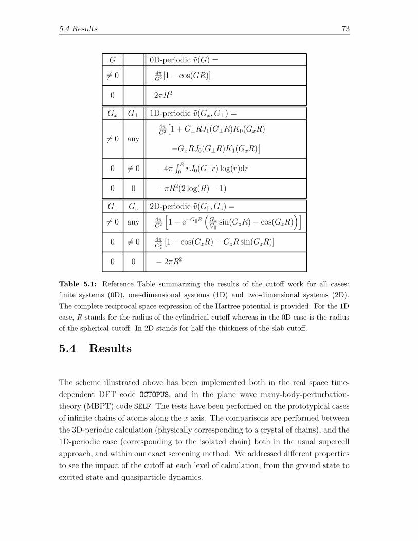
5.4 Results 73
G 0D-periodic v(G) =
6= 0 4πG2 [1 − cos(GR)]
0 2πR2
Gx G⊥ 1D-periodic v(Gx, G⊥) =
6= 0 any
4πG2
[
1 +G⊥RJ1(G⊥R)K0(GxR)
−GxRJ0(G⊥R)K1(GxR)]
0 6= 0 − 4π∫ R
0rJ0(G⊥r) log(r)dr
0 0 − πR2(2 log(R) − 1)
G‖ Gz 2D-periodic v(G‖, Gz) =
6= 0 any 4πG2
[
1 + e−G‖R(
Gz
G‖sin(GzR) − cos(GzR)
)]
0 6= 0 4πG2
z[1 − cos(GzR) −GzR sin(GzR)]
0 0 − 2πR2
Table 5.1: Reference Table summarizing the results of the cutoff work for all cases:
finite systems (0D), one-dimensional systems (1D) and two-dimensional systems (2D).
The complete reciprocal space expression of the Hartree potential is provided. For the 1D
case, R stands for the radius of the cylindrical cutoff whereas in the 0D case is the radius
of the spherical cutoff. In 2D stands for half the thickness of the slab cutoff.
5.4 Results
The scheme illustrated above has been implemented both in the real space time-
dependent DFT code OCTOPUS, and in the plane wave many-body-perturbation-
theory (MBPT) code SELF. The tests have been performed on the prototypical cases
of infinite chains of atoms along the x axis. The comparisons are performed between
the 3D-periodic calculation (physically corresponding to a crystal of chains), and the
1D-periodic case (corresponding to the isolated chain) both in the usual supercell
approach, and within our exact screening method. We addressed different properties
to see the impact of the cutoff at each level of calculation, from the ground state to
excited state and quasiparticle dynamics.

74 Chapter 5. An exact Coulomb cutoff technique for supercell calculations
5.4.1 Ground state calculations
All the ground state calculations have been done with the real-space implementation
of DFT in the OCTOPUS code. We have used non-local norm-conserving pseudopo-
tentials [Troullier 91] to describe the electron-ion interaction and the local-density
approximation (LDA)[Perdew 81] to describe exchange-correlation effects. The par-
ticular choice of exchange-correlation or ionic-pseudopotential does not matter here
as we want to assert the impact of the Coulomb cutoff and this is independent of
those quantities. Moreover, we have used a grid of 0.38 a.u. for Si and Na. In
this case the footprint of the interaction of neighboring chains in the y and z direc-
tion is the dispersion of the bands in the corresponding direction of the Brillouin
zone. However it is known that, if the supercell is large enough, the bands along
the Γ −X direction are unchanged. This is in apparent contradiction with the fact
that the radial ionic potential for a wire (that asymptotically goes like ln(r) as a
function of the distance r from the axis of the wire) is completely different from the
crystal potential. The answer to this contradiction is clear if we perform a cutoff
calculation. In fact the overall effect on the occupied states turns out to be canceled
by the Hartree potential, i.e. by the electron screening of the ionic potential, but
two different scenarios are visible as soon as the proper cutoff is used. In the top
panel of Fig. 5.3 it is shown the ionic potential, the Hartree potential, and their
sum for a Si atom in a parallelepiped supercell with side lengths of 2.5, 11, and
11 a.u. respectively in the x, y and z directions.No cutoff is used here. The ionic
potential is roughly behaving like 1r
in the area not too close to the nucleus (where
the pseudopotential takes over). The total potential, on the other hand, falls off
rapidly to an almost constant value at around 4 a.u. from the nuclear position, by
effect of the electron screening. The bottom panel of Fig. 5.3 shows the results when
the cutoff is applied (the radius of the cylinder is R = 5.5 a.u. such that there is
zero interaction between cells). The ionic potential now behaves like it is expected
for a potential of a chain, i.e. diverges logarithmically, and is clearly different from
the latter case. Nevertheless the sum of the ionic and Hartree potential is basically
the same as for the 3D-periodic system. In the static case the two band structure
are then expected, and are found to be the same, confirming that, as far as static
calculation are performed, the supercell approximation is good, provided that the
supercell is large enough (see left part of Fig. 5.4). In static calculations, then,
the use of our cutoff only has the effect of allowing us to eventually use a smaller
supercell, what provides clear computational savings. In the case of the Si-chain a
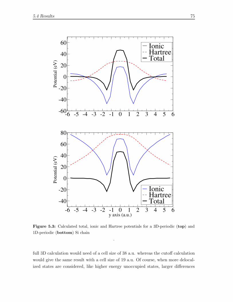
5.4 Results 75
-6 -5 -4 -3 -2 -1 0 1 2 3 4 5 6y axis (a.u.)
-60
-40
-20
0
20
40
60
Pote
ntia
l (eV
)IonicHartreeTotal
-6 -5 -4 -3 -2 -1 0 1 2 3 4 5 6y axis (a.u.)
-40
-20
0
20
40
60
80
Pote
ntia
l (eV
)
IonicHartreeTotal
Figure 5.3: Calculated total, ionic and Hartree potentials for a 3D-periodic (top) and
1D-periodic (bottom) Si chain
.
full 3D calculation would need of a cell size of 38 a.u. whereas the cutoff calculation
would give the same result with a cell size of 19 a.u. Of course, when more delocal-
ized states are considered, like higher energy unoccupied states, larger differences

76 Chapter 5. An exact Coulomb cutoff technique for supercell calculations
0 0.1 0.2 0.3 0.4 0.5qx/Gx
-15
-10
-5
0
5E-
E F (eV
)
0 0.1 0.2 0.3 0.4 0.5qx/Gx
-1
0
1
2
3
4
5
E-E F (e
V)
Figure 5.4: Left: Band structure of Si linear chain in a supercell size of 4.9x19x19 a.u.
Right: Effect of the cutoff in the band structure of a Na linear chain in a supercell size of
7.5×19×19 a.u. The bands obtained with an ordinary supercell calculation with no cutoff
(red dashed line) are compared to the bands obtained applying the 1D cylindrical cutoff
(black solid line). As it is explained in the text, only the unoccupied levels are affected by
the cutoff.
are observed with respect to the supercell calculation. In Fig. 5.4 a Na chain with
lattice constant 7.5 a.u. is considered in a cell of 7.5x19x19 a.u., and the effect of the
effect of the cutoff on the occupied and unoccupied states is shown. As expected,
the occupied states are not affected by the use of the cutoff, since the density of
the system within the cutoff radius is unchanged, and the corresponding band is the
same as it is found for an ordinary 3D supercell calculation with the same supercell
size. However there is a clear effect on the bands corresponding to the unoccupied
states, and the effect is larger the higher is the energy of the states. In fact the high
energy sates, and the states in the continuum are more delocalized, and therefore
the effect of the boundary conditions is more sensible about them.
5.4.2 Static polarizability
After the successful analysis of the ground state properties with the cutoff scheme,
we have applied the modified Coulomb potential to calculate the static polarizability
of an infinite chain in the Random Phase Approximation (RPA). As a test case we
have considered a chain made of hydrogen atoms, two atoms per cell at a distance
of 2 a.u. The lattice parameter was 4.5 a.u. For this system we have also calculated
excited state properties in many-body perturbation theory, in particular the quasi-
particle gap in Hedin’s GW approximation (section (3.3)) and the optical absorption
spectra in the Bethe-Salpeter framework (section (3.4)) (see subsections below). All

5.4 Results 77
these calculations have been performed in the code SELF. The polarizability for the
monomer in the RPA approximation including local field effects is defined as
α = − limq→0
1
q2χ00(q)
Ω
4π. (5.29)
where χGG′(q) is the interacting polarization function that is solution of the Dyson
like equation:
χGG′(q) = χ0GG′(q) +
∑
G′′
χ0GG′′(q)v(q + G′′)χG′′G′(q). (5.30)
and χ0 is the non interacting polarization function obtained by the Adler Wiser
expression Eq. (2.17) calculated for ω = 0 that now in reciprocal space reads:
χ0GG′(q, ω) = 2
∑
i,j
(fi − fj)〈j|e−i(q+G)·r|i〉〈i|ei(q+G)·r|j〉
ω − ωij + iη. (5.31)
v(q+G) are the Fourier components of the Coulomb interaction. The RPA polariz-
ability, Eq. (5.30, is equivalent to Eq. (2.18) formulated in G-space, once fxc is set
to 0. Equation (5.29) is nothing else that Eq. (2.13) in Fourier space. In the top
panel of Fig. 5.5 we compare the values of the calculated polarizability α for differ-
ent supercell sizes. α is calculated both using the bare Coulomb v(q + G) = 4π|q+G|2
and the modified cutoff potential of Eq. (5.12) (the radius of the cutoff is always
set to half the inter-chain distance). The lattice constant along the chain axis
is kept fixed. Using the cutoff the static polarizability already converges to the
asymptotic value with an inter-chain distance of 25 a.u., while without the cutoff
the convergence is much slower, and the exact value is approximated to the same
accuracy for much larger cell sizes (beyond the calculations shown in the top of
Fig. 5.5). We must stress that the treatment of the divergences in this case is
different with respect to the case of the Hartree and ionic potential cancellation
for ground-state calculations (i.e. charge neutrality). In fact, while in the calcula-
tion for the Hartree and ionic potential the diverging terms are simply dropped by
virtue of the neutralizing positive background, here we are treating only the elec-
tronic part and the h-dependence in Eq. (5.25) can be removed only for the head
component by virtue of the vanishing limit limq→0χ000(q) = 0, while for the other
Gx = 0 components we have to resort to the expression of the finite cylindrical
cutoff as in Eq. (5.25). A finite version of the 1D cutoff has been recently applied
to nanotube calculations.[Spataru 04b, Spataru 04a] This cutoff was obtained by
numerically truncating the Coulomb interaction along the axis of the nanotube, in
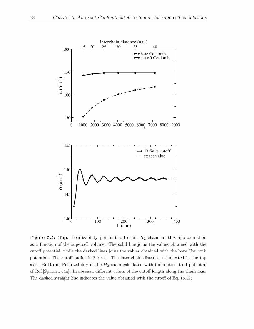
78 Chapter 5. An exact Coulomb cutoff technique for supercell calculations
0 1000 2000 3000 4000 5000 6000 7000 8000 9000supercell volume (a.u.3)
50
100
150
200
α (a
.u.3 )
15 20 25 30 35 40Interchain distance (a.u.)
bare Coulombcut off Coulomb
0 100 200 300 400h (a.u.)
140
145
150
155
α (a
.u.3 )
1D finite cutoffexact value
Figure 5.5: Top: Polarizability per unit cell of an H2 chain in RPA approximation
as a function of the supercell volume. The solid line joins the values obtained with the
cutoff potential, while the dashed lines joins the values obtained with the bare Coulomb
potential. The cutoff radius is 8.0 a.u. The inter-chain distance is indicated in the top
axis. Bottom: Polarizability of the H2 chain calculated with the finite cut off potential
of Ref.[Spataru 04a]. In abscissa different values of the cutoff length along the chain axis.
The dashed straight line indicates the value obtained with the cutoff of Eq. (5.12)
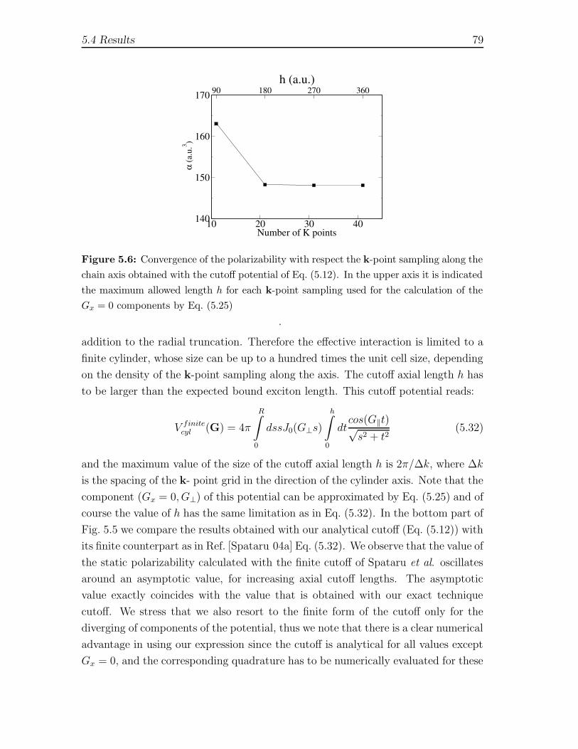
5.4 Results 79
10 20 30 40Number of K points
140
150
160
170
α (a
.u.3 )
90 180 270 360h (a.u.)
Figure 5.6: Convergence of the polarizability with respect the k-point sampling along the
chain axis obtained with the cutoff potential of Eq. (5.12). In the upper axis it is indicated
the maximum allowed length h for each k-point sampling used for the calculation of the
Gx = 0 components by Eq. (5.25)
.
addition to the radial truncation. Therefore the effective interaction is limited to a
finite cylinder, whose size can be up to a hundred times the unit cell size, depending
on the density of the k-point sampling along the axis. The cutoff axial length h has
to be larger than the expected bound exciton length. This cutoff potential reads:
V finitecyl (G) = 4π
R∫
0
dssJ0(G⊥s)
h∫
0
dtcos(G‖t)√s2 + t2
(5.32)
and the maximum value of the size of the cutoff axial length h is 2π/∆k, where ∆k
is the spacing of the k- point grid in the direction of the cylinder axis. Note that the
component (Gx = 0, G⊥) of this potential can be approximated by Eq. (5.25) and of
course the value of h has the same limitation as in Eq. (5.32). In the bottom part of
Fig. 5.5 we compare the results obtained with our analytical cutoff (Eq. (5.12)) with
its finite counterpart as in Ref. [Spataru 04a] Eq. (5.32). We observe that the value of
the static polarizability calculated with the finite cutoff of Spataru et al. oscillates
around an asymptotic value, for increasing axial cutoff lengths. The asymptotic
value exactly coincides with the value that is obtained with our exact technique
cutoff. We stress that we also resort to the finite form of the cutoff only for the
diverging of components of the potential, thus we note that there is a clear numerical
advantage in using our expression since the cutoff is analytical for all values except
Gx = 0, and the corresponding quadrature has to be numerically evaluated for these

80 Chapter 5. An exact Coulomb cutoff technique for supercell calculations
point only. In Fig. 5.6 is shown the convergences of the polarizability obtained with
our cutoff with respect to the k-points sampling. The sampling is unidimensional
along the axial direction. Using 20 k-points the calculation is already converged. In
the upper axis it is also indicated the corresponding maximum allowed value of the
finite cutoff length in the axial direction that has been used to calculate the Gx = 0
component. Finite size effects turn to be relevant also for many-body perturbation
theory calculations. For the same test system (linear H2-chain) we look in the next
two subsections to the performance of our cutoff potential for the calculation of the
quasiparticle energies in GW approximation and in the absorption spectra in the
Bethe-Salpeter framework.
5.4.3 Quasiparticles in the GW approximation
Here we show the effect of the modified cutoff potential on the calculation of the
quasiparticles energies in GW approximation for the same system studied in sec-
tion (5.4.2). We first calculate the ground state electronic properties using the DFT
code ABINIT. These calculation are performed in LDA [Perdew 81] and pseudopo-
tentials [Troullier 91] approximations. An energy cutoff of 30 Hartree has been used
to get converged results. The LDA eigenvalues and eigenfunctions are then used to
construct the RPA screened Coulomb interaction W Eq. (2.40), and the GW Self
Energy as described in Eq. (3.24). In order to eliminate the spurious interaction
between different supercells, leaving the bare Coulomb interaction unchanged along
the chain direction, we just introduce the expression of Eq. (5.12) in the construc-
tion of Σx Eq. (4.16) and Σc Eq. (4.17). The integral in the frequency domain of
Eq. (4.17) has been performed analytically using the plasmon pole approximation,
so the cutoff potential has been used also in the calculation of ε−1GG′ for the the two
frequencies needed to fit the expression of Eq. (4.18). As we did for the calculation
of the static polarizability, the divergences appearing in the components (Gx = 0)
cannot be fully removed and for such components we resort to the finite version of
the cutoff potential Eq. (5.25). In the top panel of Fig. 5.7 the convergence of the
quasiparticle gap at the X point is calculated for different supercell sizes in the GW
approximation. A cutoff radius of 8.0 a.u. has been used. When the cutoff potential
is used, 60 k-points along the axis direction has been necessary to get converged
results. In the bottom panel of Fig. 5.7 we show the behavior of the quasiparticle
gap in function of the cutoff radius We can observe that for Rc > 6a.u. a plateau
is reached and for Rc > 12a.u. small oscillation appears due to interaction between
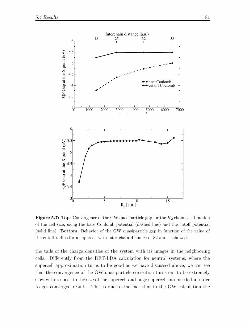
5.4 Results 81
0 1000 2000 3000 4000 5000 6000 7000supercell volume (a.u.3)
3
3.5
4
4.5
5
5.5
6
QP
Gap
at t
he X
poi
nt (e
V)
18 25 32 38Interchain distance (a.u.)
bare Coulombcut off Coulomb
0 5 10 15Rc [a.u.]
3
3.5
4
4.5
5
5.5
6
QP
Gap
at t
he X
poi
nt (e
V)
Figure 5.7: Top: Convergence of the GW quasiparticle gap for the H2 chain as a function
of the cell size, using the bare Coulomb potential (dashed line) and the cutoff potential
(solid line). Bottom: Behavior of the GW quasiparticle gap in function of the value of
the cutoff radius for a supercell with inter-chain distance of 32 a.u. is showed.
the tails of the charge densities of the system with its images in the neighboring
cells. Differently from the DFT-LDA calculation for neutral systems, where the
supercell approximation turns to be good as we have discussed above, we can see
that the convergence of the GW quasiparticle correction turns out to be extremely
slow with respect to the size of the supercell and huge supercells are needed in order
to get converged results. This is due to the fact that in the GW calculation the

82 Chapter 5. An exact Coulomb cutoff technique for supercell calculations
addition of an electron (or a hole) in the system induces charge oscillation in the
periodic images. It is important to note that the slow convergence is caused by the
correlation part of the Self-energy (Eq. (4.17)), while the exchange part is rapidly
convergent with respect to the cell size. The use of the cutoff Coulomb potential
really improves drastically the convergence as it is evident from Fig. 5.7. Notice
that still at 38 a.u. inter-chain distance the GW gap is underestimated by about
0.5 eV. A similar trend (but with smaller variations) has been found by Onida et
al. [Onida 95], for a finite system (Sodium Tetramer) using the cutoff potential of
Eq. (5.11). Clearly there is a strong dimensionality dependence of the Self-energy
correction. The non-monotonic behavior versus dimensionality of the self-energy
correction has also been point out in ref. [Delerue 03] where the gap-correction was
shown to have a strong component of the surface polarization.
5.4.4 Exciton binding energy: Bethe-Salpeter equation
Starting from the quasiparticle energies we have calculated the optical absorp-
tion spectra including electron-hole interactions solving the Bethe-Salpeter equation
(3.40). For the discussion below we consider only singlet states and only the res-
onant part of Hexc (3.44). The approximation of neglecting the coupling part of
the Excitonic Hamiltonian is well justified as we will see in the next chapter. The
quasiparticle energies entering in the diagonal part of the Hamiltonian (Eq.3.44) are
obtained applying a scissor operator to the LDA energies, because in the studied
test case the main difference between the Quasiparticle and LDA band structure
consists of a rigid energy shift of energy bands. From the solution of the BS equa-
tion (Eq.4.20) it is possible to calculate the macroscopic dielectric function from
Eq. (3.42), that when only resonant part is considered the imaginary part reduces
to:
ε2(ω) = 2 limq→0
1
q2
∑
S
Im
∣
∣
∣
∑
vckAvckS 〈vk − q|e−iq·r|ck〉
∣
∣
∣
2
ES − ω − iη, (5.33)
where the summation runs over all the vertical excitations from the ground state
to excited state ΨS, ES is the corresponding excitation energy and η is a positive
infinitesimal. As in the case of GW calculation, in order to isolate the chain, we
substitute the cutoff potential of Eq. (5.12) both in the exchange term Eq. (4.21)
and in the direct term of the BS equation Eq. (4.22), as well as for the RPA dielectric
matrix present in Eq. (4.22). In the top panel of Fig. 5.8 we show the calculated

5.4 Results 83
2 3 4 5 6 7Energy (eV)
0
500
1000
1500
2000
2500
3000
Im ε
MΩ
/4π
interchain 15 a.u.interchain 20 a.u.interchain 25 a.u.interchain 30 a.u.with cylindrical cutoffnon interacting system
0 1000 2000 3000 4000 5000 6000 7000supercell volume (a.u.3)
1
1.2
1.4
1.6
1.8
2
Bind
ing
Ener
gy (e
V)
15 20 25 30 35 38Interchain distance [a.u.]
bare Coulombcut off Coulomb
Figure 5.8: Top: Photo absorption cross section for different supercell volumes. In the
legend the inter-chain distances corresponding to each volume are indicated. The intensity
have been normalized to the volume of the supercell. The non-interacting absorption
spectra and the spectra obtained with the cutoff potential are also included. Bottom:
exciton binding energy vs supercell volume calculated using the cut off potential (solid
line), and the bare Coulomb potential (dashed line).

84 Chapter 5. An exact Coulomb cutoff technique for supercell calculations
0.5 0.55 0.6 0.65 0.7 0.75 0.8 0.85 0.9 0.95 1
0 0.1 0.2 0.3 0.4 0.5 0 0.1
0.2 0.3
0.4 0.5
0.5 0.6 0.7 0.8 0.9
1
ε00-1
qx/Gx
qy/Gy
ε00-1
0.88
0.9
0.92
0.94
0.96
0.98
1
0 0.1 0.2 0.3 0.4 0.5 0 0.1
0.2 0.3
0.4 0.5
0.5 0.6 0.7 0.8 0.9
1
ε00-1
qx/Gx
qy/Gy
ε00-1
Figure 5.9: Values of ε−100 (qx, qy) in the qz = 0 plane for the H2 chain with an inter-chain
distance of 25 a.u., using the bare Coulomb (top) and the cutoff potential (bottom). The
axis of the chain is along the x direction
spectra for different cell sizes together with the non-interacting spectrum, and the
spectrum obtained using the cutoff Coulomb potential for an inter-chain distance
larger than 20 a.u. and cylindrical cutoff radius of 8 a.u.. The scissor operator
applied in this calculation is the same for all the volumes and correspond to the
converged GW gap. As it is known, the electron-hole interaction modifies both
the shape and the energy of the main absorption peak. The present results clearly
illustrate that the spectrum calculated without the cutoff slowly converges toward
5.4 Results 85
the exact result. This is highlighted in the bottom panel of Fig. 5.8 where we show
the dependency of the exciton binding energy on the supercell volume, the binding
energy being defined as the energy difference between the excitonic peak and the
optical gap. We observe that the effect of the inter-chain interaction consists in
reducing the binding energy with respect to its value in the isolated system. This
value is slowly approached as the inter-chain distance increases, while, once the cutoff
is applied to the Coulomb potential, the limit is reached as soon as the densities of
the system and its periodical images do not interact. If we consider the convergence
of the quasiparticle gap and of the binding energy with respect to the cell volume we
notice that, if a cutoff is not used, the position of the absorption peak is controlled
by the convergence of the BS solution, which, in turn, depends on the (slower)
convergence of the GW energies. It is clear from Fig. 5.7 that the use of the cutoff
allows us to considerably speed up this bottleneck. The use of our cutoff also has
an important effect on the Brillouin zone sampling. In Fig. 5.9 we show the value of
ε−100 (qx, qy) in the qz = 0 plane for a supercell corresponding to an inter-chain distance
of 25 a.u. When the cutoff potential is used (bottom panel) the screening is smaller,
compared to the case of the bare potential (top panel). Looking at the direction
perpendicular to the chain (the chain axis is along the x direction) we see that the
dielectric matrix is approximately constant, and this fact allows us to sample the
Brillouin zone only in the direction of the chain axis. For both the GW and Bethe-
Salpeter calculations a three dimensional sampling of the Brillouin zone is needed
to get converged results when no cutoff is used, while a simple one-dimensional
sampling can be adopted when the interaction is cutoff.
5.4.5 Comparison between real-space and plane wave codes
We end this section by showing a calculation of the photo-absorption spectra of
one monomer of polyacetylene, a finite system performed as a test for the two
code employed in this thesis. The absorption spectra is calculated in TDDFT with
the ALDA approximation. One calculation is made in real space and real time as
described in section (4.1) using the code OCTOPUS, and the polarizability is given
by Eq. (2.13). The other one in the supercell approach. In reciprocal space the
same quantity is given by Eq. (5.29), and the polarization function in the ALDA
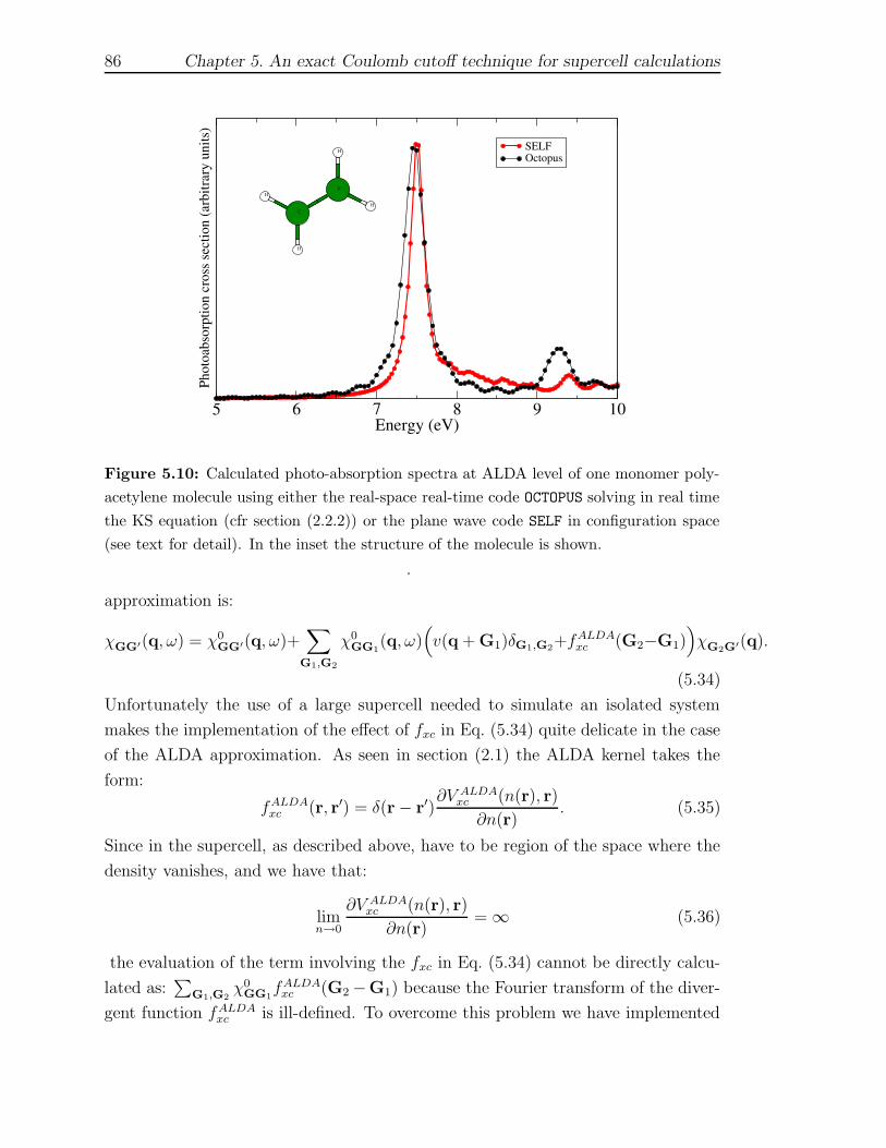
86 Chapter 5. An exact Coulomb cutoff technique for supercell calculations
5 6 7 8 9 10Energy (eV)
Phot
oabs
orpt
ion
cros
s sec
tion
(arb
itrar
y un
its)
SELFOctopus
C
CH
H
H
H
Figure 5.10: Calculated photo-absorption spectra at ALDA level of one monomer poly-
acetylene molecule using either the real-space real-time code OCTOPUS solving in real time
the KS equation (cfr section (2.2.2)) or the plane wave code SELF in configuration space
(see text for detail). In the inset the structure of the molecule is shown.
.
approximation is:
χGG′(q, ω) = χ0GG′(q, ω)+
∑
G1,G2
χ0GG1
(q, ω)(
v(q + G1)δG1,G2+fALDAxc (G2−G1)
)
χG2G′(q).
(5.34)
Unfortunately the use of a large supercell needed to simulate an isolated system
makes the implementation of the effect of fxc in Eq. (5.34) quite delicate in the case
of the ALDA approximation. As seen in section (2.1) the ALDA kernel takes the
form:
fALDAxc (r, r′) = δ(r − r′)∂V ALDA
xc (n(r), r)
∂n(r). (5.35)
Since in the supercell, as described above, have to be region of the space where the
density vanishes, and we have that:
limn→0
∂V ALDAxc (n(r), r)
∂n(r)= ∞ (5.36)
the evaluation of the term involving the fxc in Eq. (5.34) cannot be directly calcu-
lated as:∑
G1,G2χ0
GG1fALDAxc (G2 −G1) because the Fourier transform of the diver-
gent function fALDAxc is ill-defined. To overcome this problem we have implemented
5.4 Results 87
in the code SELF the solution of the TDDFT equation in ALDA approximation in the
configuration space. Similarly to the BS equation where we have written the polar-
izability in the form of Eq. (3.36) we can write the polarizability χ in configuration
space as:
χ(n1,n2)(n3,n4) =[
HALDA − Iω]−1
(n1,n2)(n3,n4)(fn4 − fn3) (5.37)
and calculate the polarizability χ by diagonalizing the ALDA Hamiltonian. Follow-
ing the same steps as we have arrived at Eq. (3.44) for the resonant part of the
excitonic Hamiltonian, now we have for the ALDA Hamiltonian:
HALDA,res(v,c)(v′ ,c′) = Hdia
(v,c)(v′ ,c′) + 2Kx(v,c)(v′ ,c′) +KALDA
(v,c)(v′ ,c′) (5.38)
where Hdia(v,c)(v′ ,c′) and Kx
(v,c)(v′ ,c′) are respectively given by Eq. (3.45a) and Eq. (4.21)
in reciprocal space, while KALDA(v,c)(v′ ,c′) is given by:
KALDA(v,c)(v′ ,c′) = 2
∫ ∫
drdr′φ∗c(r)φv(r)f
ALDAxc (r, r′)φc′(r
′)φ∗v′(r
′) (5.39)
where we have omitted the label k because for a finite system we have considered
only the Γ point. The coupling part of the Hamiltonian is written analogously to
Eq. (3.46) inverting the indexes v′, c′ → c′, v′. The term KALDA(v,c)(v′ ,c′) is evaluated
in real space, performing the Fast Fourier Transform in order to obtain the KS wave-
functions φi(r). It is important to note here that at difference of the BS equation, in
TDDFT the diagonal and the off-diagonal blocks are of the same order of magnitude,
and the off-diagonal blocks cannot be neglected. The obtained results are shown in
Fig. 5.10, together with the atomic structure of the simulated molecule. The real
space calculation has be done in a spherical simulation box of 13.5 a.u. radius and
a spacing of 0.4 a.u.. The total time of the simulation was 15 fs with a time step
of 0.001 fs. For the plane waves calculation we adopted a cubic supercell with side
of 30 a.u. and a spherical cut coulomb potential Eq. (5.11) with a cutoff radius of
12a.u. The ALDA Hamiltonian Eq. (5.38) was constructed including conduction-
valence pairs up to 27 eV (240 bands) and in the exchange part have been included
10000 plane waves (G2/2=10 Ry), in order to get converged results. We found a
good agreement between the two calculations, in particular for the first and more
relevant peak.

88 Chapter 5. An exact Coulomb cutoff technique for supercell calculations

Part III
Applications
89

6 Optical spectroscopy of
biological chromophores
Over the last years TDDFT has emerged as a very successful framework to describe
the optical spectra of small nanostructured materials, thanks to its simplicity and
moderate computational cost. It has been shown to work very well for the de-
scription of electronic excitations of a large set of molecular systems[Furche 05]:
first and second row elements as well as noble and early transition metal sys-
tems. Another major area of application is clusters, covalent and metallic, includ-
ing Met-Cars [Martinez 04]. Only recently the TDDFT has started to be used
for studying the optical response of some biomolecules and photo-biology prob-
lems e.g. chlorophylls[Sundholm 00, Sundholm 03], flavins[Neiss 03], nucleic acid
bases[Tsolakidis 05, Shukla 04], and protonated Schiff base of retinal[Tachikawa 04].
Therefore, we think it is a promising tool for the description of excited-state bio-
logical processes. It is still perhaps too soon to discuss the general level of accu-
racy of TDDFT when applied to biomolecules, especially when dealing with van
der Waals complexes [von Lilienfeld 04] and charge-transfer excitations[Dreuw 03].
Furthermore, as the field is quite recent, we can still expect rapid methodological de-
velopments, in particular the derivation of better exchange-correlation functionals.
However, the existing results are very promising, and pave the way for a broader
application of TDDFT in Biochemistry. Besides the spectacular advances in the
characterization of structural and dynamical properties of complex biomolecules by
a combination of quantum-mechanical and classical-molecular mechanics methods
(QM/MM)[Brunger 88, Laio 02], the theoretical description of the interaction of
these molecules with external time-dependent fields is very much in its infancy. In
particular, processes related to vision and photosynthesis rely on a subtle interplay
between optical absorption in the photo-active center and its decaying mechanism
through the coupling to the internal vibrational modes of the molecule, including
isomerization processes as well as coupling to the environment (hosting protein and
solvent). In this chapter we apply the TDDFT, in its real time real space implemen-
tation as described in section (2.2.2) to study optical properties for two paradigmatic
91
92 Chapter 6. Optical spectroscopy of biological chromophores
systems of broad biological interest. In section (6.1) we discuss the excited states
properties of DNA bases and some assemblies of bases in different configurations.
In this work in particular we have studied paired bases in Watson Crick and in
stacked configurations and a tetramer constituted of two paired bases. This study
has permitted to analyze the impact of the different types of interaction (hydrogen
bonding and π-stacking) in the absorption spectra of such systems. The study of
such big systems has been feasible with the real-time real-space implementation of
the TDDFT, otherwise too much computationally demanding for the traditional
methods of quantum chemistry. Next, in section (6.2) we will discuss the absorp-
tion spectra of the green fluorescent protein (GFP), that we have studied within a
quantum-mechanical molecular mechanics (QM/MM) and TDDFT approach. The
calculations turns to be in an excellent agreement with the experiments and have
permitted to relate the shape of the absorption spectra with the presence of two
different form, protonated and deprotonated, of the chromophore.
6.1 Excited states of DNA bases and their assem-
blies†
Optical absorption spectroscopy is especially important for DNA and DNA-based
compounds. These techniques were extensively applied in the last decades to these
systems to characterize their structural and dynamical properties [Ruzsicska 95,
Hernandez 04a, Daniels 76]. Traditionally, DNA molecules have always retained
a special place in scientific investigation, for biological/medical issues. Moreover
in the last years, DNA is also attracting interest for several potential applica-
tions in the field of nanotechnology, due to its stability (in solution), to its one-
dimensional character, and to the regular π-stacking, along with the unique proper-
ties of self-assembling and recognition [Porath 04, Endres 04, Nalwa 05, Coehn 05,
Di Felice 02]. In relation to nanotechnology, the determination and interpretation
of the electronic properties of nucleobases and of DNA helical arrangements are
an extremely valuable foreword, and notable multidisciplinary efforts are currently
devoted to such goals: we refer the reader to recent reviews about electronic struc-
† This section is largely an adaptation of the article: D. Varsano, R. Di Felice, M.A.L Marques
and A. Rubio: Excited states of DNA bases and their assemblies accepted in J. Phys.
Chem. B (2006). As such, the reported work includes collaboration of the rest of the authors
of the article. This paper can be downloaded from cond-mat/0603086

6.1 Excited states of DNA bases and their assemblies 93
ture calculations and possible charge motion behaviors [Porath 04, Di Felice 05].
Furthermore, the knowledge of the electronic properties, excited state lifetimes,
and ultra-violet (UV) absorption spectrum is of paramount important for our un-
derstanding, e.g., of the crucial phenomena of UV radiation-induced DNA dam-
age [Kraemer 97, Odom 01, Hernandez 05]. From this brief preamble, it is clear
that the full characterization of the optical properties of such DNA complexes is
of great interest. In order to relate the optical properties of the nucleic acids
to their structure, spatial conformation, and type of intra-molecular interactions,
a valuable preliminary step is to gain insight into the excited-state properties of
their building blocks, namely the monomeric bases, and to understand the role of
hydrogen-bonding and stacking when these monomeric units form complex assem-
blies. In their natural environment, the DNA bases are paired via hydrogen-bonds
in the so called Watson-Crick scheme [Watson 53], and are covalently bonded to
the sugar-phosphate backbone. The hydrogen-bonded base pairs interact with each
other in the typical helical arrangement by inter-plane van der Waals forces [Hall 96]
,mediated by the solvent and counter-ions. To disentangle how the different inter-
actions control the DNA dynamics upon light absorption, it is important to infer
how the isolated nucleic acid spectra is modified by their mutual interaction in the
different spatial conformations of DNA-assemblies. This is the goal of the work pre-
sented in this section: To provide a systematic study of the stacking and H-bonding
interaction effects in the optical spectra of molecular complexes formed with iso-
lated DNA-bases. As mentioned in the introduction of this chapter we undertake
this task by means of time-dependent-density functional (TDDFT) calculations.
The present study should be considered as a first step toward the understanding
and control of the excited state properties of real DNA based systems, including
solvation and environment effects to a later stage. Before studying very complex
biological-based DNA complexes it is mandatory to test the performance and pre-
dictive power of TDDFT for DNA-based systems. One of the aims of the present
work is to provide first-principles calculations of simple DNA-based systems that
can be used as reference for future developments and studies. This reference set in-
cludes the isolated DNA bases, hydrogen bonded Watson-Crick pairs, stacked bases
pairs, and a GC stacked dimer. For the isolated DNA bases there are plenty of
experimental and theoretical results concerning their optical response. We do not
carry out a full systematic analysis of all the published data for the isolated DNA-
bases, but only those more pertaining to our investigation. The wide variety of
computational tools applied to nucleobases ranges from single excitation configu-

94 Chapter 6. Optical spectroscopy of biological chromophores
ration interaction (CIS), to complete active space 2nd-order perturbation theory
(CASPT2), and includes other approaches such as multireference perturbation con-
figuration interaction (CIPSI). A review of the performance of such methods on
the nucleobases is reviewed in Ref. [Hernandez 04a], as well as relevant experimen-
tal data can be found in Refs. [Fulscher 97, Fulscher 95, Lorentzon 95]. Despite
the large number of works on the excited states of isolated DNA bases, there are
limited number of studies on base pairs and base assemblies due to their complex-
ity. Shukla and Leszczynski studied adenine-uracil [Shukla 02a], adenine-thymine
(AT) and guanine-cytosine (GC) in the Watson-Crick configuration [Shukla 02b]
at CIS the level; Sobolewski and Domcke [Sobolewski 04] studied the low lying en-
ergy part of the spectrum of GC base pairs with the more sophisticated CASPT2
technique; and Wesolowski [Wesoloswki 04] used an embedding method to study
the lowest excited state of the GC and AT pairs. Very recently, Tsolakidis and
Kaxiras [Tsolakidis 05] computed the whole absorption spectra of the GC and AT
pairs in different tautomeric forms of the nucleic acid bases in TDDFT frame-
work. Moreover, very few studies exist on the excited state properties of bases
in a stacked configuration: Jean and Hall studied fluorescent properties of dimers
of 2-aminopurine stacked with DNA bases [Jean 01] in different forms and stacked
trimers containing 2-aminopurine [Jean 02], showing the relevance of the stacked
geometries in the excited state properties and in the character of the excited state
transitions. To the best of our knowledge, the present results are the first ab-initio
calculations dealing with stacked natural bases. Still we remark that the present
results are for free standing nucleoacid-complexes, i.e., not including solvation ef-
fects. These effects are known to be more important for nπ∗ than π− π∗ type tran-
sitions [Mennucci 01, Mishra 00, Shukla 00, Fulscher 97, Shukla 02a, Shukla 02b].
This section is organized as follows: In section (6.1.1) we provide the details used
to get the structures and to compute the optical properties. In section (6.1.2) we
present our results for the isolated gas-phase nucleobases, i.e., guanine, cytosine,
adenine, thymine, and uracil, (G, C, A, T, and U, respectively) and compare with
the experiments and previous calculations existing in literature. In order to under-
stand the role of hydrogen-bonding in shifting and modifying the spectral features,
we show, in section (6.1.3), results for H-bonded Watson-Crick GC and AT base
pairs (labeled GCH and ATH, respectively). In section (6.1.4) we present results
for a GC stacked dimer (la belled GCS) that mimics the arrangement between C
and G in two consecutive planes in the real DNA double helix. We also discuss
the relative roles of π-stacking and hydrogen bonding in the optical absorption of
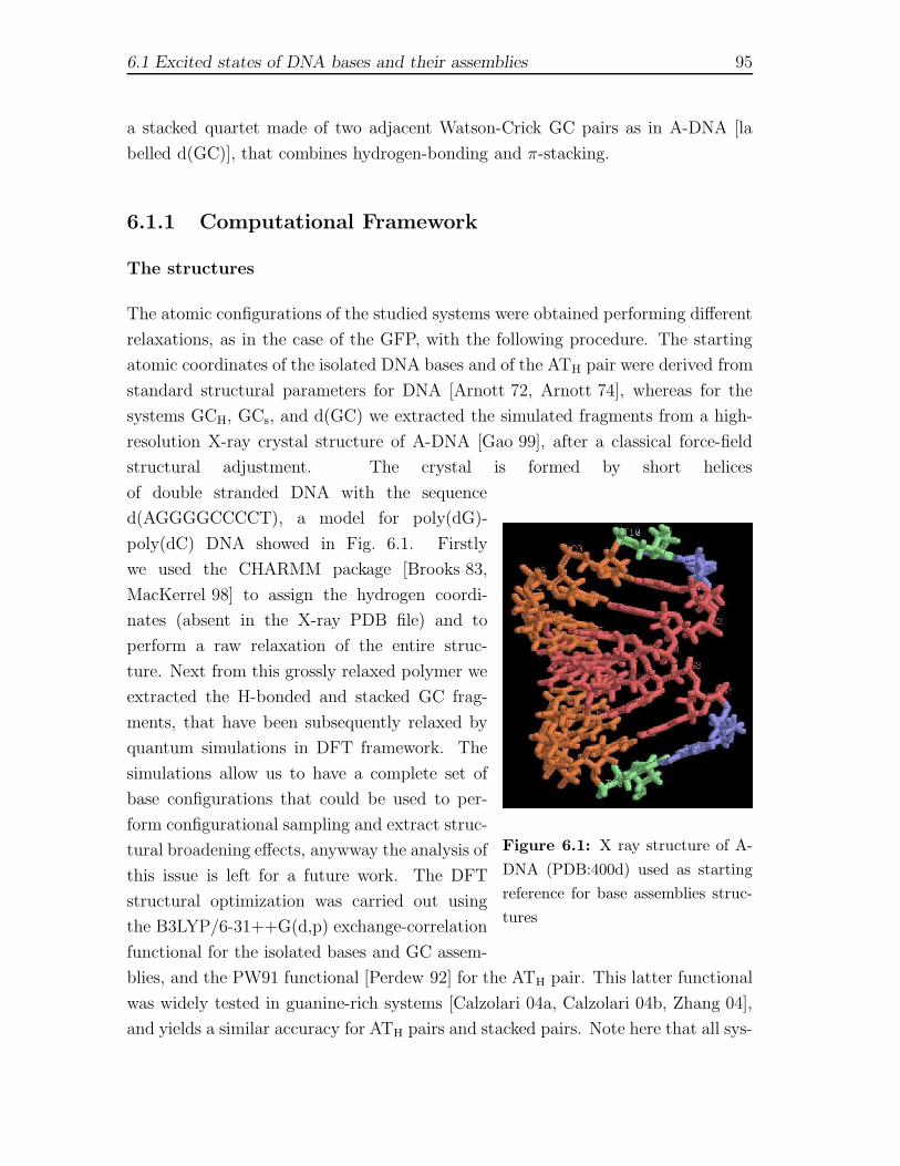
6.1 Excited states of DNA bases and their assemblies 95
a stacked quartet made of two adjacent Watson-Crick GC pairs as in A-DNA [la
belled d(GC)], that combines hydrogen-bonding and π-stacking.
6.1.1 Computational Framework
The structures
The atomic configurations of the studied systems were obtained performing different
relaxations, as in the case of the GFP, with the following procedure. The starting
atomic coordinates of the isolated DNA bases and of the ATH pair were derived from
standard structural parameters for DNA [Arnott 72, Arnott 74], whereas for the
systems GCH, GCs, and d(GC) we extracted the simulated fragments from a high-
resolution X-ray crystal structure of A-DNA [Gao 99], after a classical force-field
structural adjustment. The crystal is formed by short helices
Figure 6.1: X ray structure of A-
DNA (PDB:400d) used as starting
reference for base assemblies struc-
tures
of double stranded DNA with the sequence
d(AGGGGCCCCT), a model for poly(dG)-
poly(dC) DNA showed in Fig. 6.1. Firstly
we used the CHARMM package [Brooks 83,
MacKerrel 98] to assign the hydrogen coordi-
nates (absent in the X-ray PDB file) and to
perform a raw relaxation of the entire struc-
ture. Next from this grossly relaxed polymer we
extracted the H-bonded and stacked GC frag-
ments, that have been subsequently relaxed by
quantum simulations in DFT framework. The
simulations allow us to have a complete set of
base configurations that could be used to per-
form configurational sampling and extract struc-
tural broadening effects, anywway the analysis of
this issue is left for a future work. The DFT
structural optimization was carried out using
the B3LYP/6-31++G(d,p) exchange-correlation
functional for the isolated bases and GC assem-
blies, and the PW91 functional [Perdew 92] for the ATH pair. This latter functional
was widely tested in guanine-rich systems [Calzolari 04a, Calzolari 04b, Zhang 04],
and yields a similar accuracy for ATH pairs and stacked pairs. Note here that all sys-

96 Chapter 6. Optical spectroscopy of biological chromophores
tems studied in the present work correspond to bases in the gas phase and the effect
of a solvent may be crucial when comparing the computational results with experi-
mental data [Mennucci 01, Mishra 00]. Furthermore, the sugar-phosphate backbone
was neglected. This restriction should not be relevant in the energy range we are in-
terested in (3–7.5 eV), as the sugar and the phosphate contribution to the absorption
spectra only starts to be important above 7.0 eV.
The spectra
The optical absorption spectra of DNA bases and base pairs were computed at
TDDFT level with the code OCTOPUS [Marques 03a]. The method has been de-
scribed before in section (2.2.2) and the numerical implementation in section (4.1).
For the exchange-correlation potential vxc we employed the local density approxi-
mation (LDA) with the Perdew-Zunger parametrization [Perdew 81]. In the case
of the isolated guanine base, we also performed the time propagation with the
generalized gradient approximation (GGA) PW91 [Perdew 96] vxc functional. As
expected [Marques 01], no substantial differences were detected between the two
parameterizations. Therefore, the rest of the calculation has been performed with
the LDA functional that is numerically the most stable. Anyway it is important
here to note that in spite of the equivalence encountered in the photo-absorption
cross-section of gas-phase guanine by using these two functionals, which is suffi-
cient for our purposes to justify the LDA option, one has to be extremely careful
in general in the choice of vxc. For instance, it was shown that for processes that
involve charge transfer mechanisms, like fluorescence in base pairs, it is important
to have the correct asymptotic behavior of the exchange-correlation functional (See,
e.g. [Grimee 03]). Concerning technical details: We used a real-space grid made of
overlapping spheres centered around each nucleus with a radius of 4 A. All quanti-
ties were discretized in a uniform grid with spacing 0.23 A. The time-step for the
time evolution was 0.0066 fs (which ensures stability in the time-dependent propa-
gation of the KS wave functions) and the total propagation time was at least 20 fs.
Such simulation parameters ensure well converged absorption spectra up to about
8 eV. The energy resolution, dictated by the total simulation length by ∆E ∼ h/T ,
is better than 30meV. This set the lower limit for the linewidth of the calculated
spectra, any additional broadening is intrinsic to the system. The electron-ion in-
teraction (both in the time-dependent and time-independent DFT calculations) was
modeled by norm-conserving pseudopotentials [Troullier 91]. To compare with ex-

6.1 Excited states of DNA bases and their assemblies 97
0
0.02
0.04
0.06
0.08
0.1
4 5 6 7
S (1
/eV)
Energy (eV)
nπ* 97%
nπ* 17%πσ* 80%
πσ* 99%
πσ* 70%
πσ* 90%πσ* 30%nπ* 64%time
frequency
Figure 6.2: Dipole strength function of Cytosine along the axis perpendicular to the base
plane, calculated through the real-time propagation (blue solid curve) and in the frequency
domain [Casida 95] (green dashed curve). An artificial broadening of 0.15 eV was adopted
as an eye help to compare both time and frequency domain spectra. Note that we can
distinguish the nπ∗ character in an indisputable way only for the lowest energy peak.
At higher energy the nπ∗ character is less pure, due to the mixing of a large number of
transitions. This fact is illustrated here for cytosine, but observed for all the investigated
nucleobases.
periments where the molecules are not aligned with respect to the applied field, we
need to average the response along the three Cartesian axis [cf. Eq. (2.14)]. This
result can be directly compared to other available data and used to discriminate
among different nucleoacid conformations. However, the analysis can be taken even
further: in the case of planar molecules (isolated bases, GCH, ATH) one can eas-
ily distinguish between in-plane and out-of-plane transitions. While the former are
prevalently ππ∗ and have large oscillator strengths, the latter are much weaker (by
one or two orders of magnitude) and are usually hidden under the stronger signals.
In order to unveil the character of the weak transitions, the time-domain analysis
is not sufficient: Thus, we also performed linear response calculations in the fre-
quency domain [Casida 95], as described in section (2.2.1) for all planar structures
(isolated bases, GCH, and ATH pairs). In this formalism, several pairs of occu-
pied/unoccupied orbitals participate in each excitation with different weights: it is
then possible to qualitatively assign to each excitation the predominant character
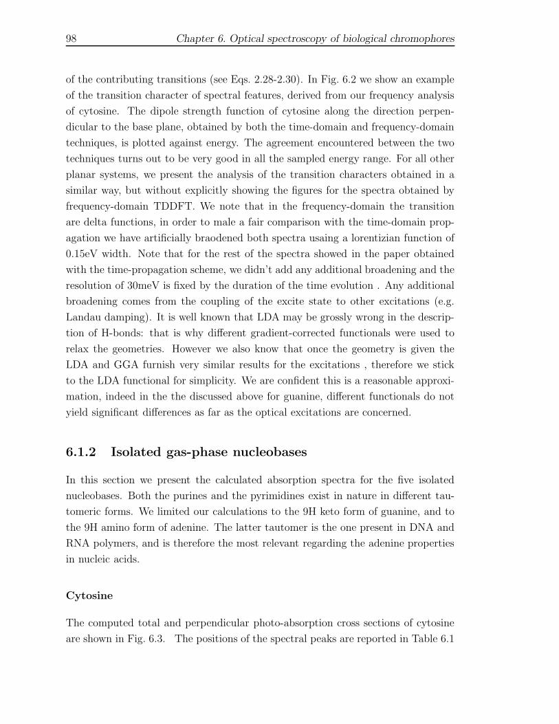
98 Chapter 6. Optical spectroscopy of biological chromophores
of the contributing transitions (see Eqs. 2.28-2.30). In Fig. 6.2 we show an example
of the transition character of spectral features, derived from our frequency analysis
of cytosine. The dipole strength function of cytosine along the direction perpen-
dicular to the base plane, obtained by both the time-domain and frequency-domain
techniques, is plotted against energy. The agreement encountered between the two
techniques turns out to be very good in all the sampled energy range. For all other
planar systems, we present the analysis of the transition characters obtained in a
similar way, but without explicitly showing the figures for the spectra obtained by
frequency-domain TDDFT. We note that in the frequency-domain the transition
are delta functions, in order to male a fair comparison with the time-domain prop-
agation we have artificially braodened both spectra usaing a lorentizian function of
0.15eV width. Note that for the rest of the spectra showed in the paper obtained
with the time-propagation scheme, we didn’t add any additional broadening and the
resolution of 30meV is fixed by the duration of the time evolution . Any additional
broadening comes from the coupling of the excite state to other excitations (e.g.
Landau damping). It is well known that LDA may be grossly wrong in the descrip-
tion of H-bonds: that is why different gradient-corrected functionals were used to
relax the geometries. However we also know that once the geometry is given the
LDA and GGA furnish very similar results for the excitations , therefore we stick
to the LDA functional for simplicity. We are confident this is a reasonable approxi-
mation, indeed in the the discussed above for guanine, different functionals do not
yield significant differences as far as the optical excitations are concerned.
6.1.2 Isolated gas-phase nucleobases
In this section we present the calculated absorption spectra for the five isolated
nucleobases. Both the purines and the pyrimidines exist in nature in different tau-
tomeric forms. We limited our calculations to the 9H keto form of guanine, and to
the 9H amino form of adenine. The latter tautomer is the one present in DNA and
RNA polymers, and is therefore the most relevant regarding the adenine properties
in nucleic acids.
Cytosine
The computed total and perpendicular photo-absorption cross sections of cytosine
are shown in Fig. 6.3. The positions of the spectral peaks are reported in Table 6.1
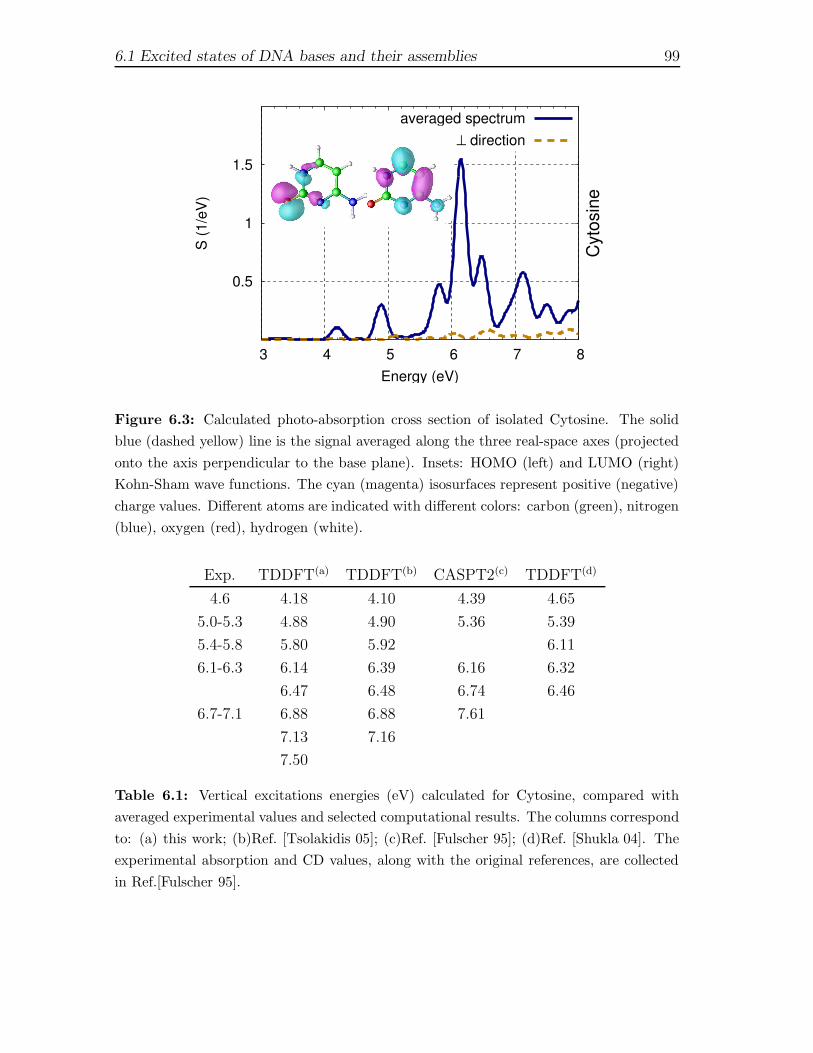
6.1 Excited states of DNA bases and their assemblies 99
1.5
1
0.5
3 4 5 6 7 8
S (1
/eV)
Cyto
sine
Energy (eV)
averaged spectrum⊥ direction
Figure 6.3: Calculated photo-absorption cross section of isolated Cytosine. The solid
blue (dashed yellow) line is the signal averaged along the three real-space axes (projected
onto the axis perpendicular to the base plane). Insets: HOMO (left) and LUMO (right)
Kohn-Sham wave functions. The cyan (magenta) isosurfaces represent positive (negative)
charge values. Different atoms are indicated with different colors: carbon (green), nitrogen
(blue), oxygen (red), hydrogen (white).
Exp. TDDFT(a) TDDFT(b) CASPT2(c) TDDFT(d)
4.6 4.18 4.10 4.39 4.65
5.0-5.3 4.88 4.90 5.36 5.39
5.4-5.8 5.80 5.92 6.11
6.1-6.3 6.14 6.39 6.16 6.32
6.47 6.48 6.74 6.46
6.7-7.1 6.88 6.88 7.61
7.13 7.16
7.50
Table 6.1: Vertical excitations energies (eV) calculated for Cytosine, compared with
averaged experimental values and selected computational results. The columns correspond
to: (a) this work; (b)Ref. [Tsolakidis 05]; (c)Ref. [Fulscher 95]; (d)Ref. [Shukla 04]. The
experimental absorption and CD values, along with the original references, are collected
in Ref.[Fulscher 95].
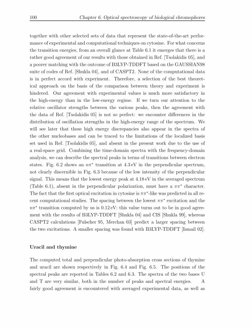
100 Chapter 6. Optical spectroscopy of biological chromophores
together with other selected sets of data that represent the state-of-the-art perfor-
mance of experimental and computational techniques on cytosine. For what concerns
the transition energies, from an overall glance at Table 6.1 it emerges that there is a
rather good agreement of our results with those obtained in Ref. [Tsolakidis 05], and
a poorer matching with the outcome of B3LYP-TDDFT based on the GAUSSIAN98
suite of codes of Ref. [Shukla 04], and of CASPT2. None of the computational data
is in perfect accord with experiment. Therefore, a selection of the best theoret-
ical approach on the basis of the comparison between theory and experiment is
hindered. Our agreement with experimental values is much more satisfactory in
the high-energy than in the low-energy regime. If we turn our attention to the
relative oscillator strengths between the various peaks, then the agreement with
the data of Ref. [Tsolakidis 05] is not so perfect: we encounter differences in the
distribution of oscillation strengths in the high-energy range of the spectrum. We
will see later that these high energy discrepancies also appear in the spectra of
the other nucleobases and can be traced to the limitations of the localized basis
set used in Ref. [Tsolakidis 05], and absent in the present work due to the use of
a real-space grid. Combining the time-domain spectra with the frequency-domain
analysis, we can describe the spectral peaks in terms of transitions between electron
states. Fig. 6.2 shows an nπ∗ transition at 4.3 eV in the perpendicular spectrum,
not clearly discernible in Fig. 6.3 because of the low intensity of the perpendicular
signal. This means that the lowest energy peak at 4.18 eV in the averaged spectrum
(Table 6.1), absent in the perpendicular polarization, must have a ππ∗ character.
The fact that the first optical excitation in cytosine is ππ∗-like was predicted in all re-
cent computational studies. The spacing between the lowest ππ∗ excitation and the
nπ∗ transition computed by us is 0.12 eV: this value turns out to be in good agree-
ment with the results of B3LYP-TDDFT [Shukla 04] and CIS [Shukla 99], whereas
CASPT2 calculations [Fulscher 95, Merchan 03] predict a larger spacing between
the two excitations. A smaller spacing was found with B3LYP-TDDFT [Ismail 02].
Uracil and thymine
The computed total and perpendicular photo-absorption cross sections of thymine
and uracil are shown respectively in Fig. 6.4 and Fig. 6.5. The positions of the
spectral peaks are reported in Tables 6.2 and 6.3. The spectra of the two bases U
and T are very similar, both in the number of peaks and spectral energies. A
fairly good agreement is encountered with averaged experimental data, as well as

6.1 Excited states of DNA bases and their assemblies 101
1.5
1
0.5
3 4 5 6 7 8
S (1
/eV)
Thym
ine
Energy (eV)
averaged spectrum⊥ direction
Figure 6.4: Calculated photo-absorption cross section of isolated Thymine. The solid
blue (dashed yellow) line is the signal averaged along the three real-space axes (projected
onto the axis perpendicular to the base plane). Insets: HOMO (left) and LUMO (right)
Kohn-Sham wave functions. The cyan (magenta) isosurfaces represent positive (negative)
charge values. Different atoms are indicated with different colors: carbon (green), nitrogen
(blue), oxygen (red), hydrogen (white).
Exp. TDDFT(a) TDDFT(b) CASPT2(c) TDDFT(d)
4.5-4.7 4.54 4.45 4.39(nπ∗) 4.69
5.0-5.1 5.30 5.24 4.88 4.96
5.8-6.0 5.74 5.68 5.88 5.95
6.3-6.6 6.36 6.38 6.10 6.19
6.51 6.50
7.0 6.88 6.86 7.13 6.86
7.07
7.21 7.28
7.59 7.52
Table 6.2: Vertical excitations energies (eV) calculated for Thymine, compared with
average experimental values and selected calculations. The columns correspond to:
(a) this work; (b) Ref. [Tsolakidis 05]; (c) Ref. [Lorentzon 95]; (d) Ref [Shukla 04].
The experimental absorption and CD values, along with the original references, are col-
lected in Ref.[Lorentzon 95], except the second experimental band that is taken from
Refs.[Miles 67, Sprecher 77].
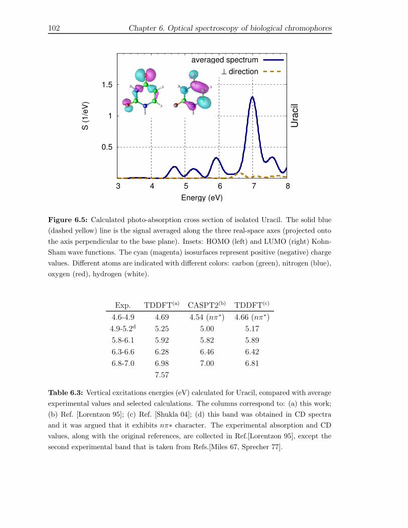
102 Chapter 6. Optical spectroscopy of biological chromophores
1.5
1
0.5
3 4 5 6 7 8
S (1
/eV)
Urac
il
Energy (eV)
averaged spectrum⊥ direction
Figure 6.5: Calculated photo-absorption cross section of isolated Uracil. The solid blue
(dashed yellow) line is the signal averaged along the three real-space axes (projected onto
the axis perpendicular to the base plane). Insets: HOMO (left) and LUMO (right) Kohn-
Sham wave functions. The cyan (magenta) isosurfaces represent positive (negative) charge
values. Different atoms are indicated with different colors: carbon (green), nitrogen (blue),
oxygen (red), hydrogen (white).
Exp. TDDFT(a) CASPT2(b) TDDFT(c)
4.6-4.9 4.69 4.54 (nπ∗) 4.66 (nπ∗)
4.9-5.2d 5.25 5.00 5.17
5.8-6.1 5.92 5.82 5.89
6.3-6.6 6.28 6.46 6.42
6.8-7.0 6.98 7.00 6.81
7.57
Table 6.3: Vertical excitations energies (eV) calculated for Uracil, compared with average
experimental values and selected calculations. The columns correspond to: (a) this work;
(b) Ref. [Lorentzon 95]; (c) Ref. [Shukla 04]; (d) this band was obtained in CD spectra
and it was argued that it exhibits nπ∗ character. The experimental absorption and CD
values, along with the original references, are collected in Ref.[Lorentzon 95], except the
second experimental band that is taken from Refs.[Miles 67, Sprecher 77].
6.1 Excited states of DNA bases and their assemblies 103
with TDDFT [Tsolakidis 05, Shukla 04] and CASPT2 [Lorentzon 95] computational
data. All previous calculations, either in the TDDFT framework or with quantum
chemistry methods, predict the lowest transition to have an nπ∗ character in vacuo.
We agree with this assignment for uracil (the perpendicular signal is not visible at
4.69 eV in Fig. 6.5 due to the weak intensity). In the case of thymine, we do not find
any appreciable signal perpendicular to the base plane contributing to the peak at
4.54 eV. However, this is consistent with TDDFT calculations of Ref. [Shukla 04] and
CASPT2 of Ref. [Lorentzon 95], as they indeed report nπ∗ transitions with extremely
small oscillation strengths (1e-4–1e-6), unresolved by us. The character of the band
at 4.9–5.2 eV for uracil and at 5.0–5.1 eV for thymine is not yet clear: the absorption
spectra of uracil compounds [Clark 65] and circular dichroism experiments [Miles 67]
indicate that it is due to a ππ∗ transition. However, such ππ∗ character has not
been confirmed by magnetic circular dichroism [Voelter 68] and polarized absorption
spectra experiments [Stewart 63, Stewart 64, Fucaloro 71, Eaton 70]. Lorentzon and
coworkers [Lorentzon 95], by performing calculations at the CASPT2 level, suggest
that this band has nπ∗ origin: they arrived at this conclusion by correcting their
computed values with a 0.5 eV blue-shift due to the solvent. A similar conclusion
was reported for uracil by Shukla and coworkers [Shukla 00], who performed CIS
calculations taking the solvent into account with a polarizable continuum model.
However, more recently, Shukla and Leszczynski [Shukla 04] using B3LYP-TDDFT
reported only a ππ∗ transition at 5.17 eV for uracil and at 4.96 for thymine in the
energy range under consideration. In our work, we do not detect any absorption in
the direction perpendicular to the base-plane in this energy range, whereas peaks at
5.24 eV for T and at 5.25 eV for U are found, with considerable oscillator strength
induced by light polarized in the plane of the molecule. Therefore, our results
indicate that the second band is most likely to have a ππ∗ character.
Adenine
The computed total and perpendicular photo-absorption cross sections of 9H-adenine
are shown in Fig. 6.6. The positions of the spectral peaks are summarized in Ta-
ble 6.4 and compared with other available theoretical and experimental data. An
excellent agreement with other LDA-TDDFT computed values [Tsolakidis 05] is ob-
served, regarding both the peak energies and the relative oscillation strengths. Slight
discrepancies occur only in the high energy range, as these are most likely due to
differences in the technical details adopted in the calculations (e.g., the basis sets).

104 Chapter 6. Optical spectroscopy of biological chromophores
1.5
1
0.5
3 4 5 6 7 8
S (1
/eV)
Aden
ine
Energy (eV)
averaged spectrum⊥ direction
Figure 6.6: Calculated photo-absorption cross section of isolated Adenine. The solid
blue (dashed yellow) line is the signal averaged along the three real-space axes (projected
onto the axis perpendicular to the base plane). Insets: HOMO (left) and LUMO (right)
Kohn-Sham wave functions. The cyan (magenta) isosurfaces represent positive (negative)
charge values. Different atoms are indicated with different colors: carbon (green), nitrogen
(blue), oxygen (red), hydrogen (white).
Looking at the spectrum in the direction perpendicular to the base plane, we can
distinguish four prevalently nπ∗ transitions in the energy range 4.10–4.79 eV, that
are hidden in Fig. 6.6 because of their tiny oscillator strengths. We find that the
lowest excitation has mainly nπ∗ character and is very close in energy to the first ππ∗
transition (forming the peak at 4.51 eV). This result is in agreement with resonant
two-photon ionization and laser induced fluorescence spectroscopy of jet cooled ade-
nine [Kim 00], provided that the adiabatic transition energies follow the same trends
as the calculated vertical ones. Our findings also agree qualitatively with frequency-
domain B3LYP-TDDFT [Shukla 04] and CIPSI [Mennucci 01, Sobolewski 02] cal-
culations, whereas CASPT2 [Fulscher 97] and CIS [Holmen 97, Broo 98, Mishra 00]
yield the reverse order. Given the small energy difference between the two transi-
tions we can conclude that the overall qualitative agreement is satisfactory. Pro-
ceeding to higher energies, we find the second ππ∗ peak 0.37 eV after the first
one. Experiments indicate [Holmen 97, Callis 64, Clark 95] that the low energy
portion of the adenine photo-absorption spectrum consists of two closely spaced
6.1 Excited states of DNA bases and their assemblies 105
Exp. TDDFT (a) TDDFT(b) CASPT2(c) TDDFT(d)
4.59 4.51 4.51 5.13 4.94
4.8-4.9 4.88 4.95 5.20 5.21
5.38 5.49 5.58
5.7-6.1 5.72 5.79 6.24 5.93
6.26 6.19 6.28 6.72 6.12
6.49 6.63 6.16
6.81 6.76 6.92 6.99
7.09 7.47
7.73 7.39 7.81 7.57
Table 6.4: Vertical excitations energies (eV) calculated for Adenine, compared with av-
eraged experimental values and selected calculations. The columns correspond to: (a) this
work; (b) Ref. [Tsolakidis 05]; (c) Ref. [Fulscher 97]; (d) Ref. [Shukla 04]. The exper-
imental absorption and CD values, along with the original references, are collected in
Ref.[Fulscher 97].
ππ∗ transitions. Holmen and coworkers showed by linear dichroism that those two
peaks are separated by 0.26 eV. This value is in reasonable agreement with our re-
sults and with other TDDFT calculations [Mennucci 01, Tsolakidis 05], while other
computational results obtained with different techniques predict a closer energy
spacing. On the other hand, measured spectra indicate that the lowest energy
transition has a smaller oscillator strength than the subsequent one: such an ev-
idence is consistent with the CASPT2 and CIPSI results, whereas TDDFT simu-
lations [Tsolakidis 05] yield an inverse ordering of oscillator strengths in the first
two peaks (see Fig. 6.6). Concerning other nπ∗ transitions, there is experimental
evidence by circular [Sprecher 77, Brunner 75] and linear [Holmen 97] dichroism of
a signal around 5.4 eV. Our calculation is also able to reveal a signal in this range.
However, the agreement with the experiment for the nπ∗ transitions should be con-
sidered with caution, because of their high sensibility to the effect of the solvent
(neglected in our calculations) and exchange-correlation functional.
Guanine
To conclude the presentation of the results for the isolated DNA bases, we show in
Fig. 6.7 the computed total and perpendicular photo-absorption cross sections of
9H-guanine. The positions of the spectral peaks are summarized in Table 6.5 and
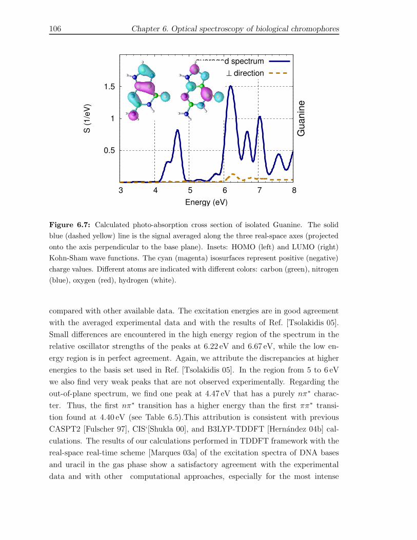
106 Chapter 6. Optical spectroscopy of biological chromophores
1.5
1
0.5
3 4 5 6 7 8
S (1
/eV)
Gua
nine
Energy (eV)
averaged spectrum⊥ direction
Figure 6.7: Calculated photo-absorption cross section of isolated Guanine. The solid
blue (dashed yellow) line is the signal averaged along the three real-space axes (projected
onto the axis perpendicular to the base plane). Insets: HOMO (left) and LUMO (right)
Kohn-Sham wave functions. The cyan (magenta) isosurfaces represent positive (negative)
charge values. Different atoms are indicated with different colors: carbon (green), nitrogen
(blue), oxygen (red), hydrogen (white).
compared with other available data. The excitation energies are in good agreement
with the averaged experimental data and with the results of Ref. [Tsolakidis 05].
Small differences are encountered in the high energy region of the spectrum in the
relative oscillator strengths of the peaks at 6.22 eV and 6.67 eV, while the low en-
ergy region is in perfect agreement. Again, we attribute the discrepancies at higher
energies to the basis set used in Ref. [Tsolakidis 05]. In the region from 5 to 6 eV
we also find very weak peaks that are not observed experimentally. Regarding the
out-of-plane spectrum, we find one peak at 4.47 eV that has a purely nπ∗ charac-
ter. Thus, the first nπ∗ transition has a higher energy than the first ππ∗ transi-
tion found at 4.40 eV (see Table 6.5).This attribution is consistent with previous
CASPT2 [Fulscher 97], CIS‘[Shukla 00], and B3LYP-TDDFT [Hernandez 04b] cal-
culations. The results of our calculations performed in TDDFT framework with the
real-space real-time scheme [Marques 03a] of the excitation spectra of DNA bases
and uracil in the gas phase show a satisfactory agreement with the experimental
data and with other computational approaches, especially for the most intense

6.1 Excited states of DNA bases and their assemblies 107
Exp. TDDFT a TDDFTb CASPT2c TDDFTd
4.4-4.5 4.40 4.46 4.76 4.85
4.9-5.0 4.66 4.71 5.09 5.11
5.01 5.04
5.28
5.7-5.8 5.76 5.64 5.96 5.59
6.1-6.3 6.22 6.23 6.55 5.83
6.6-6.7 6.67 6.53 6.65
6.66
6.82 6.77
7.04 6.93
7.58 7.26
Table 6.5: Vertical excitations energies (eV) calculated for Guanine, compared with av-
eraged experimental values and selected calculations. The columns correspond to: (a) this
work; (b) Ref. [Tsolakidis 05]; (c) Ref. [Fulscher 97]; (d) Ref. [Shukla 04]. The exper-
imental absorption and CD values, along with the original references, are collected in
Ref.[Fulscher 97].
peak above 6 eV. In particular, good agreement is found with recent LDA-TDDFT
calculations using a localized-basis set [Tsolakidis 05]. Minor differences are found
regarding the distribution of the oscillator strengths in the high energy range of
the spectra. Such discrepancies can be ascribed to the different basis sets used
in the calculations: a uniform grid in real space in this work, and a set of local-
ized atomic orbitals in Ref. [Tsolakidis 05]. Regarding the more problematic nπ∗
transitions, we found that the weak perpendicular signal is sometimes hidden be-
low the in-plane signal. In the cases where the nπ∗ transitions can be detected,
we found the correct relative ordering between nπ∗ and ππ∗ peaks, as compared
with other TDDFT calculations performed in the frequency domain. Another in-
teresting trend is the relative ordering among different nucleobases for what con-
cerns the first ππ∗ transition. For this feature, supersonic jet experiments report
C < G < A [Kim 00, Mons 02, Nir 02]. We indeed find that ordering in our first-
principles calculations, i.e. the first excitation at 4.18 eV for cytosine, 4.40 eV for
guanine and at 4.52 eV for adenine. Last, we note that our calculations give the
expected characters of the Kohn-Sham orbitals of the different bases (see insets
in Figs. 6.3-6.7): the LUMO has π character for all the nucleobases, whereas the
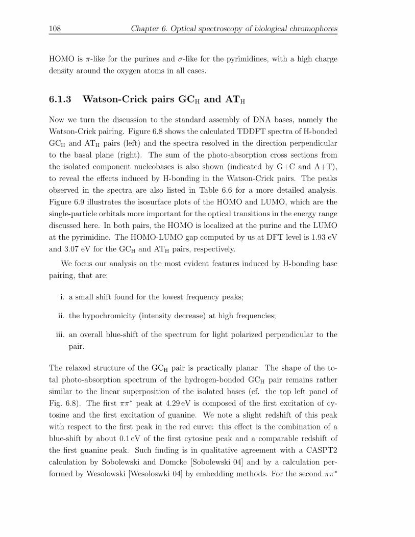
108 Chapter 6. Optical spectroscopy of biological chromophores
HOMO is π-like for the purines and σ-like for the pyrimidines, with a high charge
density around the oxygen atoms in all cases.
6.1.3 Watson-Crick pairs GCH and ATH
Now we turn the discussion to the standard assembly of DNA bases, namely the
Watson-Crick pairing. Figure 6.8 shows the calculated TDDFT spectra of H-bonded
GCH and ATH pairs (left) and the spectra resolved in the direction perpendicular
to the basal plane (right). The sum of the photo-absorption cross sections from
the isolated component nucleobases is also shown (indicated by G+C and A+T),
to reveal the effects induced by H-bonding in the Watson-Crick pairs. The peaks
observed in the spectra are also listed in Table 6.6 for a more detailed analysis.
Figure 6.9 illustrates the isosurface plots of the HOMO and LUMO, which are the
single-particle orbitals more important for the optical transitions in the energy range
discussed here. In both pairs, the HOMO is localized at the purine and the LUMO
at the pyrimidine. The HOMO-LUMO gap computed by us at DFT level is 1.93 eV
and 3.07 eV for the GCH and ATH pairs, respectively.
We focus our analysis on the most evident features induced by H-bonding base
pairing, that are:
i. a small shift found for the lowest frequency peaks;
ii. the hypochromicity (intensity decrease) at high frequencies;
iii. an overall blue-shift of the spectrum for light polarized perpendicular to the
pair.
The relaxed structure of the GCH pair is practically planar. The shape of the to-
tal photo-absorption spectrum of the hydrogen-bonded GCH pair remains rather
similar to the linear superposition of the isolated bases (cf. the top left panel of
Fig. 6.8). The first ππ∗ peak at 4.29 eV is composed of the first excitation of cy-
tosine and the first excitation of guanine. We note a slight redshift of this peak
with respect to the first peak in the red curve: this effect is the combination of a
blue-shift by about 0.1 eV of the first cytosine peak and a comparable redshift of
the first guanine peak. Such finding is in qualitative agreement with a CASPT2
calculation by Sobolewski and Domcke [Sobolewski 04] and by a calculation per-
formed by Wesolowski [Wesoloswki 04] by embedding methods. For the second ππ∗
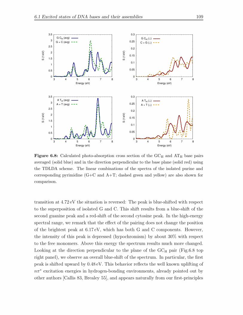
6.1 Excited states of DNA bases and their assemblies 109
0
0.5
1
1.5
2
2.5
3
3.5
3 4 5 6 7 8
S (1
/eV)
Energy (eV)
G CH (avg)G + C (avg)
0
0.05
0.1
0.15
0.2
0.25
0.3
3 4 5 6 7 8
S (1
/eV)
Energy (eV)
G CH (⊥)C + G (⊥)
0
0.5
1
1.5
2
2.5
3
3.5
3 4 5 6 7 8
S (1
/eV)
Energy (eV)
A TH (avg)A + T (avg)
0
0.05
0.1
0.15
0.2
0.25
0.3
3 4 5 6 7 8
S (1
/eV)
Energy (eV)
A TH (⊥)A + T (⊥)
Figure 6.8: Calculated photo-absorption cross section of the GCH and ATH base pairs
averaged (solid blue) and in the direction perpendicular to the base plane (solid red) using
the TDLDA scheme. The linear combinations of the spectra of the isolated purine and
corresponding pyrimidine (G+C and A+T; dashed green and yellow) are also shown for
comparison.
transition at 4.72 eV the situation is reversed: The peak is blue-shifted with respect
to the superposition of isolated G and C. This shift results from a blue-shift of the
second guanine peak and a red-shift of the second cytosine peak. In the high-energy
spectral range, we remark that the effect of the pairing does not change the position
of the brightest peak at 6.17 eV, which has both G and C components. However,
the intensity of this peak is depressed (hypochromism) by about 30% with respect
to the free monomers. Above this energy the spectrum results much more changed.
Looking at the direction perpendicular to the plane of the GCH pair (Fig.6.8 top
right panel), we observe an overall blue-shift of the spectrum. In particular, the first
peak is shifted upward by 0.48 eV. This behavior reflects the well known uplifting of
nπ∗ excitation energies in hydrogen-bonding environments, already pointed out by
other authors [Callis 83, Brealey 55], and appears naturally from our first-principles
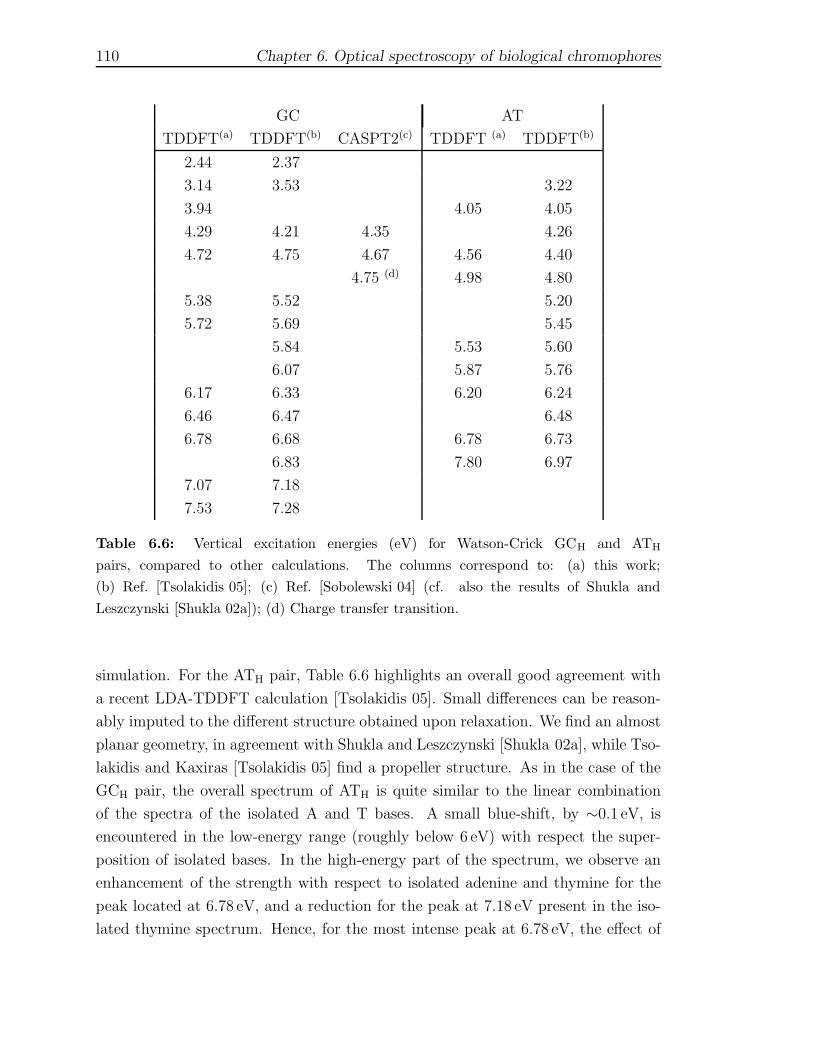
110 Chapter 6. Optical spectroscopy of biological chromophores
GC AT
TDDFT(a) TDDFT(b) CASPT2(c) TDDFT (a) TDDFT(b)
2.44 2.37
3.14 3.53 3.22
3.94 4.05 4.05
4.29 4.21 4.35 4.26
4.72 4.75 4.67 4.56 4.40
4.75 (d) 4.98 4.80
5.38 5.52 5.20
5.72 5.69 5.45
5.84 5.53 5.60
6.07 5.87 5.76
6.17 6.33 6.20 6.24
6.46 6.47 6.48
6.78 6.68 6.78 6.73
6.83 7.80 6.97
7.07 7.18
7.53 7.28
Table 6.6: Vertical excitation energies (eV) for Watson-Crick GCH and ATH
pairs, compared to other calculations. The columns correspond to: (a) this work;
(b) Ref. [Tsolakidis 05]; (c) Ref. [Sobolewski 04] (cf. also the results of Shukla and
Leszczynski [Shukla 02a]); (d) Charge transfer transition.
simulation. For the ATH pair, Table 6.6 highlights an overall good agreement with
a recent LDA-TDDFT calculation [Tsolakidis 05]. Small differences can be reason-
ably imputed to the different structure obtained upon relaxation. We find an almost
planar geometry, in agreement with Shukla and Leszczynski [Shukla 02a], while Tso-
lakidis and Kaxiras [Tsolakidis 05] find a propeller structure. As in the case of the
GCH pair, the overall spectrum of ATH is quite similar to the linear combination
of the spectra of the isolated A and T bases. A small blue-shift, by ∼0.1 eV, is
encountered in the low-energy range (roughly below 6 eV) with respect the super-
position of isolated bases. In the high-energy part of the spectrum, we observe an
enhancement of the strength with respect to isolated adenine and thymine for the
peak located at 6.78 eV, and a reduction for the peak at 7.18 eV present in the iso-
lated thymine spectrum. Hence, for the most intense peak at 6.78 eV, the effect of
6.1 Excited states of DNA bases and their assemblies 111
HOMO LUMO
+-,/. 02143
576/8 92:<;
Figure 6.9: HOMO and LUMO Kohn-Sham wave functions of the GCH (top) and ATH
(bottom) pairs. The cyan (magenta) isosurfaces represent positive (negative) charge val-
ues. Different atoms are indicated with different colors: carbon (green), nitrogen (blue),
oxygen (red), hydrogen (white).
H-bonding is contrary to the hypochromicity described above for the GCH pair. In
the out-of-plane spectrum (bottom right panel of Fig. 6.8), as for the GCH pair,
we observe that the effect of hydrogen bonding is an overall blue-shift. In particu-
lar, the first peak (that has an nπ∗ character) is shifted by 0.4 eV; the second and
fourth peaks are upward shifted by 0.2 eV and 0.3 eV respectively; the energy of the
third peak is practicallyunchanged. In addition to the above features that originate
from the individual base that eneter each pair, new features appear in the spectra
because the purine and the pyramidine coexist in the Watson-Crick arrangement.
This coexistence changes the nature of the frontier orbitals: The HOMO is purine-
localized, the LUMO is pyrimidine-localized, and the value of the HOMO-LUMO
gap is smaller than in the isolated bases. Consequently, peaks at lower energies
emerge in the spectra: they are reported in Table VI, but the corresponding energy
range is not shown in the figures, because the tiny oscillator strengths make them
undiscernible from the more intense peaks. We also note that the extremely small
intensity makes the quantitative assignment of these features less reliable than the
others already discussed. In the case of GCH, we find excitation energies at 2.44
eV, 3.14 eV and 3.94 eV, with oscillator strengths of 0.001, 0.008 and 0.003. These

112 Chapter 6. Optical spectroscopy of biological chromophores
oscillator strengths are two orders of magnitude smaller than the peak at 4.29 eV
shown in the upper panel of Fig. 6.8. For the ATH pair, the lowest energy peak
at 4.05 eV has an oscillator strength of 0.048. This transition has a small com-
ponent also in the absorption for light polarized perpendicular to the base plane
(see bottom right panel in Fig. 6.8). Its origin can be likely ascribed to charge
transfer states, that have received particular attention from both experimental and
theoretical viewpoints [Jortner 98]. However, we warn the reader that the identifi-
cation of charge transfer transitions is to be taken with care at the current level of
TDDFT when a local or gradient-corrected exchange-correlation functional is used
[Dreuw 03, Dreuw 04, Gritsenko 04].
6.1.4 Stacked GCs and d(GC) structures
With the results reported in the previous section for the GCH pair, we can un-
derstand what happens in the optical absorption when a guanine and a cytosine
dimerize through hydrogen bonding. Here, the GCs system is selected to check
which effects arise when the same two bases dimerize in a different form, namely
by stacking. Fig. 6.10 reports the averaged and direction-resolved spectra of the
stacked GCs dimer. The comparison between Figs. 6.10 and 6.8 aims at disclosing
the relative role of hydrogen-bonding and π-stacking in the optical response of nu-
cleobase complexes. We also plot in Fig. 6.10 the linear combination of the spectra
of the isolated constituent bases. Fig. 6.11 (top) illustrates the Kohn-Sham highest
occupied and lowest unoccupied orbitals of the system. It is important to note that
both the HOMO and the LUMO have charge density distributed around both the
purine and the pyrimidine, at odds with the H-bonded GCH pair (compare Fig. 6.9,
top) where the HOMO is centered at the purine and the LUMO at the pyrimidine.
As in the case of hydrogen-bonding, the shape of the spectrum it is not strongly
altered, but important differences are encountered in the oscillator strengths. Look-
ing at the first peaks at low energy, we see that the excitations due to the cytosine
moieties are slightly blue-shifted (as for the GCH pair), while the guanine excitations
appear not be affected. The resulting spectrum below 5 eV is made of two equally
intense closely spaced peaks at 4.45 eV and 4.68 eV, whereas in the H-bonded GCH
structure we observed two well separated peaks spaced by 0.4 eV and with different
intensities. Hypochromicity is also observed in this low-energy range, whereas for
the GCH pair hypochromicity occurs only in the high-energy range. In the range be-
tween 5 and 6 eV, we find an intensity enhancement of the weak peak at 5.31 eV and
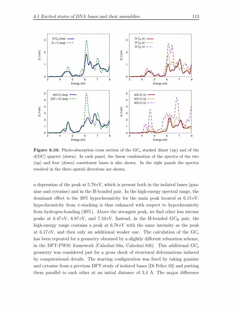
6.1 Excited states of DNA bases and their assemblies 113
0
1
2
3
3 4 5 6 7 8
S (1
/eV)
Energy (eV)
G CS (avg)G + C (avg)
0
1
2
3
3 4 5 6 7 8
S (1
/eV)
Energy (eV)
G CS (x)G CS (y)G CS (z)
0
1
2
3
4
5
6
3 4 5 6 7 8
S (1
/eV)
Energy (eV)
d(G C) (avg)2(G + C) (avg)
0
1
2
3
4
5
6
3 4 5 6 7 8
S (1
/eV)
Energy (eV)
d(G C) (x)d(G C) (y)d(G C) (z)
Figure 6.10: Photo-absorption cross section of the GCs stacked dimer (up) and of the
d(GC) quartet (down). In each panel, the linear combination of the spectra of the two
(up) and four (down) constituent bases is also shown. In the right panels the spectra
resolved in the three spatial directions are shown.
a depression of the peak at 5.78 eV, which is present both in the isolated bases (gua-
nine and cytosine) and in the H-bonded pair. In the high-energy spectral range, the
dominant effect is the 39% hypochromicity for the main peak located at 6.15 eV:
hypochromicity from π-stacking is thus enhanced with respect to hypochromicity
from hydrogen-bonding (30%). Above the strongest peak, we find other less intense
peaks at 6.47 eV, 6.87 eV, and 7.10 eV. Instead, in the H-bonded GCH pair, the
high-energy range contains a peak at 6.78 eV with the same intensity as the peak
at 6.17 eV, and then only an additional weaker one. The calculation of the GCs
has been repeated for a geometry obtained by a slightly different relaxation scheme,
in the DFT-PW91 framework [Calzolari 04a, Calzolari 04b]. This additional GCs
geometry was considered just for a gross check of structural deformations induced
by computational details. The starting configuration was fixed by taking guanine
and cytosine from a previous DFT study of isolated bases [Di Felice 02] and putting
them parallel to each other at an initial distance of 3.4 A. The major difference

114 Chapter 6. Optical spectroscopy of biological chromophores
HOMO LUMO
=?>A@
BDCFE
GIHKJ
GIHKJ
LNMAO
LNMAO
Figure 6.11: Isosurface plots of the HOMO and LUMO Kohn-Sham wave functions of
the GCs π-stacked dimer (top) and of the d(GC) π-stacked quartet (bottom). The cyan
(magenta) isosurfaces represent positive (negative) charge values. Different atoms are
indicated with different colors: carbon (green), nitrogen (blue), oxygen (red), hydrogen
(white).
PDB 400d+CHARMM+B3LYP Ref. [Di Felice 02] + PW91
Figure 6.12: Two different conformations obtained for the π-staked GCs pair obtained
by different structural relaxation schemes.
between the two GCs structures (Fig. 6.12) is the tilt angle, which is smaller in the
PW91 relaxation. The two spectra are quite similar in both shape and intensity:
minor differences are observed only in the the first peak, that is shifted upward by
0.15 eV in the structure shown in the right panel of Fig. 6.12. The combined effects

6.1 Excited states of DNA bases and their assemblies 115
of stacking and H-bonding on the absorption spectra are simultaneously present in
Fig. 6.10 (lower panel), that corresponds to two stacked GCH pairs with the G’s on
the same strand of the parent polymer [Gao 99]. The shape of the spectrum appears
very similar to that of a single GCH pair (Fig. 6.8, top left), but the intensity of
all peaks is reduced. Such decrease is a typical qualitative effect of the stacking ar-
rangement, although the molecular details fix the quantitative aspects (we described
the stacking between guanine and cytosine above, whereas we are now focusing on
the stacking between two guanines). In fact, in the low-energy range we find again
very slight shifts for the first two peaks, downward for the first and upward for the
second, as in Fig. 6.8 (top left). However, the intensity of the second peak is equal
to that obtained from the G+C combination, whereas in the single GCH pair it
was higher. This is due to a depression of the second peak (guanine) induced by
stacking. In the high-energy range, the hypochromicity due to both the π-stacking
and the H-bonding couplings is confirmed. For the main peak located at 6.25 eV
we find an intensity reduction by 62% with respect to the free monomers. The two
kinds of base couplings seem to act separately and independently, in the sense that
one does not affect the other: such separation was already reported concerning the
electronic structure [Di Felice 02]. Summarizing this section, we have shown that
stacked and H-bonded GC pairs present slight differences in the absorption spectra,
both in the low-energy and high-energy ranges. Hypochromicity has been found in
both configurations and results to be largest for the stacked pairs. Hypochromicity
is very useful because this intensity change can be used to follow the melting of the
secondary structure of nucleic acids when varying the temperature or environmental
parameters.
Conclusion
In conlcusion we presented a complete study of the optical absorption spectra of the
five isolated gas-phase nucleobases and their assemblies: simple Watson-Crick pairs,
simple π-stacking of two bases and more complex π-stacks Watson-Crick GC pairs.
These calculations of isolated simple nucleobase-assemblies are a remarkable play-
ground to prove the reliability of TDDFT for DNA-based materials. Remarkably, for
the first time the optical properties were computed by an ab-initio method for a he-
lical conformation of two stacked GC pairs, where H-bonding and π-stacking effects
are active simultaneously and can be distinguished. The results can be summarized
as follows.

116 Chapter 6. Optical spectroscopy of biological chromophores
i. For the isolated bases we get spectra in good agreement with previous theo-
retical works and (qualitatively) with experiments.
ii. We reproduce the proper ordering of the ππ∗ excitations, namely that the
excitation energy increases in going from C to G to A.
iii. The LUMO state has always a π-like character whereas the HOMO is π-like
for the purines and σ-like for the pyrimidines.
iv. As concerns the base assemblies (Watson-Crick H-bond pairs and stacked con-
figuration), we obtain that the shape of the spectrum is not much altered by
the π-stacking or H-bond interactions. However, we always get hypochromic-
ity in the high energy range of the spectrum. This hypochromicity is enhanced
in the π-stacked case with respect the the H-bonded case.
v. For light polarized perpendicular to the bases we get a blue-shift of the spectra
compared to the spectra of the isolated bases.
vi. In the stacked case, the HOMO and LUMO states are distributed both on
the purine and pyrimidine bases, whereas in the H-bonded configuration the
HOMO is in the purine and the LUMO in the pyrimidine (charge transfer-type
excitation).
vii. When combining both H-bonding and π-stacking, the two effects add indepen-
dently, and the hypochromicity in the UV is enhanced.
Anyway it is important to note that all our calculations are in the gas phase,
which means that solvent and environment effects are not taken into account.
This hinders a direct comparison with experimental data, as most of the avail-
able results correspond to nucleobases-assemblies in solution. However, several
experimental and theoretical studies (including simplified models of the solvent)
showed that the ππ∗ transitions are only slightly affected by the presence of the
solvent [Mennucci 01, Mishra 00, Shukla 02a]: precisely , they are insensitive to
the polarity of the solvent, but may undergo red-shifts. On the contrary the
“dark” nπ∗ transitions turn out to be significanlty sensible to the polarity of the
solvent [Mennucci 01, Mishra 00, Shukla 00, Fulscher 97, Shukla 02a, Shukla 02b].
As shown in Figs. 6.3-6.7, the absorption spectra of the DNA-bases is extremely
anisotropic, due to their quasi-planar structure. Consequently, nearly all the os-
cillator strength is concentrated on the ππ∗ transition (orders of magnitude more

6.1 Excited states of DNA bases and their assemblies 117
intense than the nπ∗ transitions). Those transitions are excited only for light po-
larized in the base plane. Therefore, the present results can be used to discriminate
(albeit qualitatively) which features are mostly limited to the gas phase (those polar-
ized out-of-plane) and which ones can be considered intrinsic to the DNA-complex.
Furthermore, the role of charge-transfer states observed for instance in the ATH
spectrum needs of be analyzed more in detail in order to understand their impact
in the excited state dynamics of DNA-based complexes (note that those states are
very likely to be dark, or with very low oscillator strength for light-induced elec-
tronic excitations). Besides the optical absorption results presented in this work,
there is another optical technique that is widely used for the characterization of
chiral biomolecules – circular dichroism. The technique used in the present work
allows for a straightforward calculation of the rotatory power or circular dichroism
spectra keeping the simplicity of the time-propagation scheme, i.e, without the need
for empty states (see section (2.2.2) Eq.(2.34) and Ref. [Yabana 99b] for the details).
The implementation and computation of circular dichroism spectra by TDDFT could
in principle allow the identification of helical fingerprint in the optical characteris-
tics, and more direct interpretation of standard post-synthesis experimental data.
Work along this line is presently being done. 1
1 D. Varsano, R. Di Felice, M. A. L. Marques and A. Rubio Unpublished
118 Chapter 6. Optical spectroscopy of biological chromophores
6.2 The Green Fluorescent Protein (GFP)†
The Green Fluorescent Protein (GFP) is a paradigmatic case of biological system
where a biological process rely on the interplay between optical absorption of its
photo-active center and its coupling to internal vibrational modes and to the en-
vironment (hosting protein). GFP is a protein produced by a jellyfish Aequorea
that lives in the North Pacific. Its peculiarity is that it is a bio-luminescent pro-
tein that absorb ultraviolet light and emits in the lower green portion of the visible
spectrum. This molecule has become a unique tool in molecular biology due to
its fluorescence and inertness when attached to other proteins[Sullivan 99] and has
become a well established tool as a marker of gene expression and protein target-
ing in intact cells organism. GFP consists of 238 amino acids folded in a β-sheet
barrel conformation. The barrel is a quasi perfect cylinder of 42 A of height and
24 A of diameter. In the interior of the β barrel there is the central helix and the
chromophore. In Fig. 6.13 the secondary structure of the GFP (left panel) and
the atomic structure of the chromophore (left panel) The chromophore is formed by
Ser65, Tyr66 and Gly67. Ser65 is chemically modified, (its carbonyl carbon is linked
to the nitrogen of Gly67 and the carbonyl oxygen is eliminated) such that the chro-
mophore consists of two consecutive rings, the phenol-type ring of Tyr66 and a five
membered heterocyle (imidazoline) formed by the backbone of Tyr66, the carbonyl
carbon of Ser65 and the nitrogen of the backbone of Gly67. The tyroxyl hydroxyl
group is part of a complex hydrogen bond network that depending on the environ-
ment favors its protonated (neutral) or deprotonated (anionic) form. The optical
absorption spectrum of the wild type (wt)-GFP, measured at 1.6K, shows two main
resonances at 2.63 and 3.05 eV[Creemers 99, Creemers 00] that are attributed to
the two thermodynamically stable protonation states of the chromophore (negative
and neutral configurations, respectively). The equilibrium between those two states
can be controlled by external factors such as pH and by mutations that affect the
chromophore environment[Creemers 99, Creemers 00, Brejc 97, Haupts 98]. Nowa-
days there is an ample set of GFP-mutants with absorption and emission bands
ranging from the violet to the red part of the spectrum. Excitation at either fre-
† This section is largely an adaptation of the article: M.A.L. Marques, X. Lopez, D. Varsano,
A. Castro and A. Rubio: Time dependent density-functional approach for biological
chromophore: the case of the green fluorescent protein. Phys. Rev. Lett. 90 258101
(2003). As such, the reported work includes collaboration of the rest of the authors of the
article.
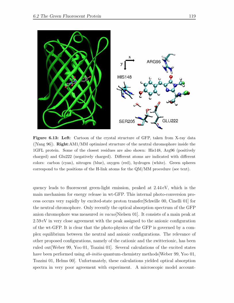
6.2 The Green Fluorescent Protein 119
Figure 6.13: Left: Cartoon of the crystal structure of GFP, taken from X-ray data
([Yang 96]). Right:AM1/MM optimized structure of the neutral chromophore inside the
1GFL protein. Some of the closest residues are also shown: His148, Arg96 (positively
charged) and Glu222 (negatively charged). Different atoms are indicated with different
colors: carbon (cyan), nitrogen (blue), oxygen (red), hydrogen (white). Green spheres
correspond to the positions of the H-link atoms for the QM/MM procedure (see text).
quency leads to fluorescent green-light emission, peaked at 2.44 eV, which is the
main mechanism for energy release in wt-GFP. This internal photo-conversion pro-
cess occurs very rapidly by excited-state proton transfer[Schwille 00, Cinelli 01] for
the neutral chromophore. Only recently the optical absorption spectrum of the GFP
anion chromophore was measured in vacuo[Nielsen 01]. It consists of a main peak at
2.59 eV in very close agreement with the peak assigned to the anionic configuration
of the wt-GFP. It is clear that the photo-physics of the GFP is governed by a com-
plex equilibrium between the neutral and anionic configurations. The relevance of
other proposed configurations, namely of the cationic and the zwitterionic, has been
ruled out[Weber 99, Yoo 01, Tozzini 01]. Several calculations of the excited states
have been performed using ab-initio quantum-chemistry methods[Weber 99, Yoo 01,
Tozzini 01, Helms 00]. Unfortunately, these calculations yielded optical absorption
spectra in very poor agreement with experiment. A microscopic model account-

120 Chapter 6. Optical spectroscopy of biological chromophores
ing for the optical properties of the GFP chromophore including its blinking and
photo-bleaching dynamics is still missing[Schwille 00, Cinelli 01]. In the present
work we prove that a combination of a quantum-mechanics/molecular mechanics
method (QM/MM) to obtain the structural properties and time-dependent density
functional theory (TDDFT) to treat the electronic excitations provides a very good
description of the optical properties of the GFP in vacuo. In the following section we
shortly describe the the QM/MM method used to obtain the structure of the chro-
mophore and we give the technical details of the calculation, while in section (6.2.2)
we give the obtained results.
6.2.1 Computational Framework
Biological systems, such as proteins, nucleic acids etc. are constituted for a big num-
ber of atoms, so that turns to be computationally impossible to perform a complete
quantum mechanical description with the methods described above. Nevertheless,
in many situations only a small part of the whole system, the chromophore, is the re-
sponsible of the UV optical absorption of the system, so we can resort to the TDDFT
limiting the calculation to the subsystem of interest. Anyway, as mentioned before,
the starting point for a TDDFT calculation is the ground state wave function usually
calculated via standard DFT schemes that of course requires the knowledge of the
structure of the system. So, even if we are interested in only a small portion of the
system, in order to have a correct description of its structure, turns to be important
to consider all the whole system because the interaction between the chromophore
and the near atoms could play an important role in its structural properties. To
take into account such interactions a viable method is the hybrid technique called
QM/MM (Quantum Mechanics Molecular Mechanics)[Brunger 88, Laio 02]. Such
method is an approximate technique that permit to treat the reacting center of
a big molecule with Quantum mechanical method, whereas the remaining part is
treated in classical way via empirical potential (See left part of Fig.(6.14)). In the
QM/MM framework the Hamiltonian of the system is given by the sum of the terms
representing the QM region, the MM region and the interaction between them:
Heff = HQM/QM + HMM/MM + HQM/MM (6.1)
HQM/QM is the Hamiltonian describing the nuclei and electrons in the quantum
region, such term can be solved using different quantum methods as DFT, Hartree
Fock or semi-empirical methods.

6.2 The Green Fluorescent Protein 121
Active site
Protein environment
QM
MM
M
M
M2
3 Q
1
Q2
Q
3
H1
Figure 6.14: Left: Scheme of the division of the system in the QM/MM framework.
Right: Schematic picture of the border between the classical and quantum part of the
system.
HMM/MM is a molecular mechanics Hamiltonian, the atoms are treated classically
and it depends only on the atoms position. The entire region is treated with force
fields. The force fields describe either the interaction among bonded atoms depend-
ing on the stretching, bending and the torsion of the bond, either the electrostatic
and Van der Waals interaction among the non-bonded atoms.
HQM/MM describes the interaction between the classical and quantum regions and
can be decomposed as:
HQM/MM = HelecQM/MM + HvdW
QM/MM + HbondedQM/MM (6.2)
The first term take into account the electrostatic interaction between the electrons
and nuclei of the quantum region with the classical part, in this treatment the atoms
of the classical part are treated as external point charges. The second term describe
the Van Der Waals interaction between the QM atoms and MM atoms and finally
the third term represent the interaction at the border. This term is introduced
when the border is inside a molecule and contains the classical field terms of the
MM atoms bonded to QM atoms. In many situation the border pass through a
covalent bond. There exist different technique to model such bond when it is a
single bond [Reuter 00], while to treat multiple bonds turns to be problematic due
to their sensibility to polarizability effects. In this work we have used the method
called link-atom. In this method each time that the border pass through a bond the
QM and MM part are connected via an hydrogen atom (see right part of Fig.6.14).
The ’artificial’ hydrogen atom is included in the quantum region, but does not
interact in electrostatic way with the classical region, furthermore this H-atom is
forced to be aligned in the direction of the bond of the border during the relaxation
of the system.

122 Chapter 6. Optical spectroscopy of biological chromophores
The structures
The GFP structures were prepared according to the following protocol. The X-
ray structure (1.9 A resolution) of the GFP from Ref.[Yang 96] (PDB code: 1GFL)
illustrated in the left panel of Fig 6.13 was taken as the reference structure. In
the X-ray structure, several water positions were identified. In the preparation of
the structures, we only kept the water molecules that lied within 6 A of the chro-
mophore. All other crystallographic water molecules were deleted. The position of
the hydrogens were initially obtained using the HBUILD command[Brunger 88] of
CHARMM[Brooks 83, MacKerrel 98]. In order to relax the geometry of the sys-
tem 3 consecutive optimizations were carried out. An initial optimization was per-
formed with all backbone and chromophore atoms fixed at their crystallographic
positions. Non-bonded interactions were treated using a spherical cutoff of 12 A
with an atom-based potential shift method for the van der Waals terms and the
force-shift method for the electrostatic terms. The system was minimized using
the steepest descent and adaptive basis Newton-Raphson minimization algorithms
[Brooks 83, MacKerrel 98]. In a second step we allowed relaxation only of the co-
ordinates of the chromophore. As the GFP chromophore (specially the imidazoline
heterocycle) does not correspond to the typical structure adopted by serine, tyrosine
or glycine, there is a lack of specific force field parameters. Therefore, we performed
this step within a QM/MM hybrid method[Field 90], using the AM1 semi-empirical
Hamiltonian[Dewar 95] to describe the quantum subsystem. The QM region was de-
fined by three amino-acids, Ser65, Tyr66 and Gly67, and the frontier between QM
and MM regions was treated within the H-link approximation. In this approach a
H atom is included whenever the frontier between the QM and MM regions passes
through a chemical bond. This H-link atom is forced during the minimization to be
aligned with the frontier bond, and does not interact with the MM atoms. In order
to avoid the QM/MM frontier to be in the C(O)-N peptide bond the carbonyl group
of Gly67 was removed from the QM subsystem and the carbonyl group of i Phe64
was included. In this way, the two H-link atoms cut through C-C bonds. Finally,
from this geometry we performed a full relaxation allowing the chromophore and
every protein atom within 10 A of the chromophore to relax. The final structure
of the chromophore with the most important neighbors residues is depicted in the
right panel of Fig. 6.13. We checked the minimization, by computing the forces
on the final geometry using a DFT scheme for the quantum part of the QM/MM
Hamiltonian[Marques 03a]. The anionic form of the chromophore was prepared
6.2 The Green Fluorescent Protein 123
from deprotonation of the Tyr66 and protonation of Glu222. The proton transfer
is mediated through a water molecule and Ser205. The water molecule, depicted
in Fig. 6.13 (right panel), receives a proton from Tyr66 and donates a proton to
Ser205, which in turn donates its original proton to Glu222. As a result, Glu222 is
neutralized. The role of the protein backbone is important for the structural relax-
ation of the anionic form. The main structural difference to the neutral form is the
relative orientation of the Tyr66-ring with respect to the imidazoline heterocycle:
In the neutral form the two ring planes are found to be slightly displaced from pla-
narity, the Cα-Cβ-Cγ-Cδ dihedral being -10.9o. In the anionic form the co-planarity
of the two rings is enhanced, through the reduction of the Cα-Cβ-Cγ-Cδ dihedral to
-1.8o. Concerning bond distances, the largest change upon deprotonation of Tyr66
corresponds to the shrinking of the C-O(H) bond distance from 1.38 A in the neu-
tral form to 1.28 A in the anionic form. From these relaxed structures, we extracted
the quantum-mechanical subsystems, that we subsequently used for out TDDFT
calculations.
The absorption spectra
The absorption spectra of the chromophore has been calculated in the same frame-
work of the DNA basis described in the previous section. The electron-ion interaction
is described through norm-conserving pseudo-potentials[Troullier 91, Kleiman 82],
and exchange-correlation effects we treated within the local-density approximation
[Ceperley 80]. We stress that in the present study the specific form of the exchange-
correlation functional should not introduce major modifications[Marques 01]. This
is, however, untrue for studies of charge-transfer processes and isomerization mech-
anisms.
6.2.2 Results
The computed spectra of the neutral and anionic conformations of the GFP chro-
mophore are given in Fig. 6.15, together with the experimental spectrum of the
wt-GFP. The spectra are averaged over the three spatial directions. Light polar-
ized along the “x”-direction is responsible for the lowest optical transition (see the
inset of Fig. 6.15), and corresponds to a π-π∗ transition between the HOMO and
LUMO orbitals of both neutral and anionic forms. The molecule is nearly trans-
parent to visible light polarized along the other two orthogonal directions. GFP

124 Chapter 6. Optical spectroscopy of biological chromophores
turns out to be a rather anisotropic molecule in the visible, property that can be
used to enhance the photo-dynamical processes in well oriented GFP samples for
opto-electronic devices. The differences between the LUMO and HOMO eigenvalues,
sometimes taken as a estimate for the HOMO-LUMO excitation energy, are respec-
tively 2.19 and 1.61 eV, for the neutral and anionic structures. It is common practice
to use these values as estimations of the physical excitations. This leads, in the case
of the GFP, to a very bad agreement with experiment. However, in TDDFT the
difference of one-particle eigenvalues is renormalized by the Coulomb and exchange-
correlation terms[Fiolhais 03, Onida 02]. Once these effects are included, the main
excitation peaks for the neutral and anionic forms move to 3.01 and 2.67 eV respec-
tively. These values are now in really good agreement with the measured excitation
energies, located at 3.05 and 2.63[Creemers 99, Creemers 00]. The π-π∗ excitations
are no longer pure HOMO-LUMO transitions and include contributions from virtual
particle-hole excitations involving several occupied and unoccupied states. Some of
the most relevant states are depicted in Fig. 6.16. The oscillator strength of the π-π∗
transition is larger in the anionic than in the neutral GFP. It is, however, possible to
obtain a quantitative description of the spectra of the wt-GFP by assuming a ∼ 4:1
ratio for the concentration of the neutral/anionic forms. This ratio is very close to
the estimated experimental ratio of 80% neutral and 20% anionic[Sullivan 99]. The
measured peaks can be clearly assigned to either the neutral or anionic forms of
the GFP. The suggested three-state model of the wt-GFP photo-physics contains
the two thermodynamically stable neutral and anionic configurations, and an un-
stable intermediate state that apparently corresponds to the anionic chromophore
in a non-equilibrium protein environment[Brejc 97]. Other intermediate state relax-
ation processes through cis-trans isomerization and a new protonated zwitterionic
form have also been proposed[Weber 99]. Our calculations give further support to
the predominance of the neutral and anionic forms in wt-GFP in agreement with
the analysis of the infrared spectra[Yoo 01, Tozzini 01]. This sustains the proposed
proton shuttle mechanism between the protonated and de-protonated forms of the
chromophore, through the corresponding charged states of the Glu222 residue where
the proton-shuttle ends. Furthermore, the structural differences between the two an-
ionic structures is very small, and changes the main absorption peak by ∼0.1 eV,
which is of the same order as the precision of our calculations. The cationic confor-
mation is derived from the neutral form by protonation on the imidazoline nitrogen
that is formally double bonded to a carbon in the neutral state. Its spectrum con-
sist of a major peak at 2.8 eV in relative agreement with the measured value for

6.2 The Green Fluorescent Protein 125
2 3 4 5Energy (eV)
σ (a
rb. u
nits)
2 3 4 5
xyz
Figure 6.15: The computed photo-absorption cross-section, σ, compared to the experi-
mental measurement. The dashed line corresponds to the neutral chromophore, the dot-
ted line to the anionic, whereas the green and blue curves are the experimental results
of Ref. [Nielsen 01] and Ref. [Creemers 99, Creemers 00] respectively. For comparative
purposes, we divided the anionic results by 4 with respect to the neutral results. In-
set: decomposition of the computed spectra of the neutral species in the three directions,
showing the inherent anisotropy of the GFP molecule.
a model chromophore in aqueous solution, 3.15 eV[Bell 00]. This predictive power
can prompt the use of TDDFT combined with time-resolved optical spectroscopy
to map the concentration of the different GFP forms in solution upon excitation,
and extract information on the isomerization paths and lifetimes of the initial and
transition states. The fact that the computed absorption spectra of the isolated
chromophore is in close agreement with the measured spectra points to an efficient
electrostatic shielding of the chromophore by the rigid β-barrel. This justifies the
comparison between in vacuo and in vivo spectra[Nielsen 01]. In spite of the rigid-
ity of the β-barrel, there is a change in the neutral/anionic concentration ratio with
temperature, glycerol content of the solution, and external pH[Sullivan 99]. This
fact can be understood by considering that the Tyr66 hydroxyl points toward the
protein surface and it is H-bonded to a water molecule, are therefore sensitive to bulk
proton concentrations. In particular the raise of the anionic population as the pH is
increased can be understood in terms of the protonation of Glu222 residue. In fact,
replacing the Ser65 by several mutants can lead to the suppression of the anionic
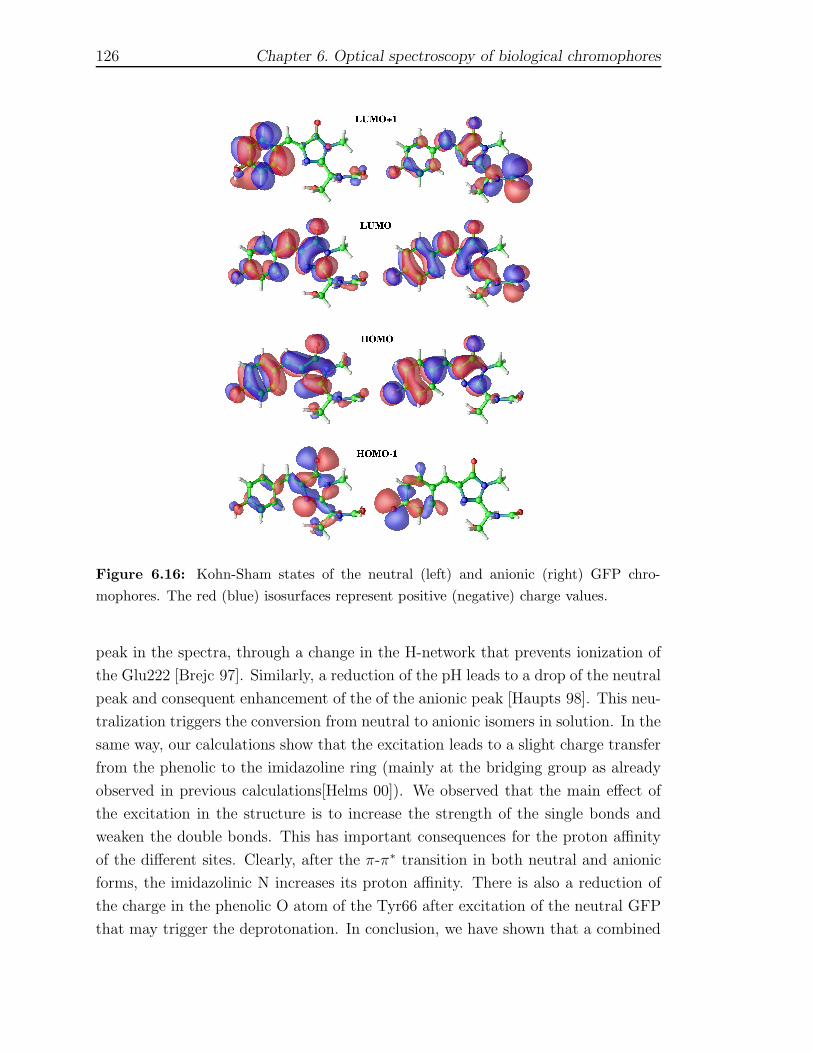
126 Chapter 6. Optical spectroscopy of biological chromophores
Figure 6.16: Kohn-Sham states of the neutral (left) and anionic (right) GFP chro-
mophores. The red (blue) isosurfaces represent positive (negative) charge values.
peak in the spectra, through a change in the H-network that prevents ionization of
the Glu222 [Brejc 97]. Similarly, a reduction of the pH leads to a drop of the neutral
peak and consequent enhancement of the of the anionic peak [Haupts 98]. This neu-
tralization triggers the conversion from neutral to anionic isomers in solution. In the
same way, our calculations show that the excitation leads to a slight charge transfer
from the phenolic to the imidazoline ring (mainly at the bridging group as already
observed in previous calculations[Helms 00]). We observed that the main effect of
the excitation in the structure is to increase the strength of the single bonds and
weaken the double bonds. This has important consequences for the proton affinity
of the different sites. Clearly, after the π-π∗ transition in both neutral and anionic
forms, the imidazolinic N increases its proton affinity. There is also a reduction of
the charge in the phenolic O atom of the Tyr66 after excitation of the neutral GFP
that may trigger the deprotonation. In conclusion, we have shown that a combined

6.2 The Green Fluorescent Protein 127
QM/MM and TDDFT approach is able to reproduce the optical response of the
GFP 1. This is a major step toward the first-principles description of excited-state
dynamic of important biological photo-receptors. Transient and time-resolved opti-
cal spectroscopy could be studied. However, in spite of the good agreement, some
questions remain open. For example, how does the excitation in the GFP trigger the
proton shuttle mechanism and what is the time-scale for this process? To answer
these questions we have to go beyond the present work where only the QM sub-
system was considered to obtain the optical response. The proton-transfer involves
structural modifications of the environment that have to be properly described by
a modified QM/MM approach. For this, the standard QM/MM methods[Laio 02]
have to be generalized to cope with excited state dynamics, and eventually to include
the possibility of charge transfer between the QM to the MM parts.
1 Similar good agreement has been obtained for other mutants of the GFP chromophore, in
particular the blue fluorescent protein [Lopez 05]

128 Chapter 6. Optical spectroscopy of biological chromophores
7 Optical absorption of quasi 1D
systems †
The application showed in the previous chapters have shown that TDDFT is a fast
and reliable tool for the description of excited states for different class of finite sys-
tems. In particular we have seen in sections (6.1 and 6.2) the good performance of
the method for the studied biological systems, and in general as asserted above it
has be shown to give results in quite good agreement for a variety of nanostructured
materials[Furche 05]. Moreover we will show in chapter 8 how TDDFT can be used
as a tool for the study of systems under the influence of strong laser fields, in partic-
ular for the study of photo-electron spectroscopy problems. In this chapter, on the
other hand, we concentrate on a paradigmatic case in which TDDFT, when applied
with standard exchange-correlation functionals (ALDA or AGGA), fails dramati-
cally. The optical absorption of long quasi one-dimensional molecular chains, calcu-
lated with local density approximation or gradient corrected functionals, gives wrong
results and the static axial polarizability and hyper-polarizability of long chains are
overestimated by orders of magnitudes when compared with experiments and cal-
culation of quantum chemistry as configuration interaction methods. As stated
in section (2.1), TDDFT is an exact reformulation of the many body Schrodinger
equation, so the failure of the theory, for this class of systems, has to be attributed
to the approximation made in practical applications: i.e. the exchange-correlation
(xc) potential used for the ground state calculation, and the time-dependent xc-
potential/kernel used for the excited state calculation. This failure is related to the
so-called ultra non-locality problem, discussed in section (1.2.2), i.e. to the strong
non-local dependence of the exchange-correlation potential when an electric field is
applied [van Gisbergen 99, Gritsenko 01]. The reason of the failure of the ALDA is
indeed its spatial locality in the xc kernel. Since the LDA depends explicitely on
† This section is largely an adaptation of the article: D. Varsano, A. Marini and A. Rubio:
Excitonic properties of quasi 1D systems: from finite chains to infinite polymers to
be published. As such, the reported work includes collaboration of the rest of the authors of the
article.
129

130 Chapter 7. Optical absorption of quasi 1D systems
Figure 7.1: Left:Axial polarizability per oligomer of polyacetylene calculated in ALDA
and VK [van Faassen 02], Hartree Fock [Kirtman 95] and MP2 [Toto 95] approximations.
Right: The same quantities calculated for H2 hydrogen, compared with coupled Hartree
Fock, MP4 and coupled cluster CCSD(T) [Champagne 95a] methods. Figures adapted
from Ref.[van Faassen 02].
the density, the ALDA kernel at the center of the molecule will be insensitive to the
variation of the density at the end-side of the chain induced by the electric field,
while for the exact exchange correlation potential this end side charge contributes
to the counteracting electric field described in section (1.2.2) that increase linearly
along all the chain. In Fig. 7.1, adapted from Ref.[van Faassen 02] it is illustrated
how wrong the LDA behaves for the axial static polarizability of two systems, the
polyacetylene and an H2n chain, as a function of the polymer length. We observe
that the error of the ALDA increase with the length of the polymer when compared
with accurate MP2 calculation, for polyacetylene and MP4 calculation for the hy-
drogen chain. A way to take into account the macroscopic polarization is by using
information coming from the induced current density rather than the density, as in
principle it is easy to mimic those effects with local functional of the current whereas
they should be extremely non local for functionals of the density. M. van Faassen et
al.[van Faassen 02] studied the axial polarizability of different polymers solving the
response equations within the Time Dependent Current Density Functional Theory
(TDCDFT), using a current-response kernel proposed by Vignale and Kohn (VK-
kernel) [Vignale 96]. These results, are shown in Fig.7.1, labeled as VK. We see
that this approach gives very good results for the polyacetylene , and in general for
131
π-conjugated systems[van Faassen 03]. However in the right panel of the figure we
observe that in the case of the H2n chain, where the dominant contribution of the
induced current comes from the polarized σ bonds, this method gives only a small
improvement with respect the ALDA result. A correct behavior of the xc electric
field and consequently a correct behavior of the static polarizability is given by or-
bital dependence functionals, in particular the simlpe one based on a exact exchange
treatment. 1 Sanchez et al. [Sanchez 03] obtained very good results for polyethi-
lene, polythiophene and the hydrogen chains. In order to get the correct behavior
of the polarizability one has to solve the cumbersome OEP equation (1.25), because
approximation to this equation as the KLI [Krieger 92] and the CEDA [Gruning 02]
partially correct the local density (LDA) and gradient corrected (GGA) approxima-
tions, but polarizabilities are still significantly larger than Hartree Fock and EXX
[Kummel 04, Gruning 02]. However we mention that for infinite systems, empirical
cutoffs are introduced to construct the fxc in exact exchange [Kim 02a, Kim 02b],
that somehow account for the screening of the electron-hole interaction. Therefore
it is important to address the issue of including screening consistenly. This is the
goal of the present chapter. We study these two system, the polyacetylene as proto-
type of a π-conjugated system and the model H2n chain in the TDDFT framework
using the new developed frequency-dependent non-local fxc kernel described in sec-
tion (3.5). We look at the optical properties of finite chains in function of the length
in both MBPT and TDDFT with this new kernel. We also address the limit of
infinite chains. In practise all these systems are studied using a plane wave basis set
with the supercell approximation with the truncated Coulomb potential described
in chapter 5. In particular to avoid spurious cel-cell interactions we cut the coulomb
potential outside a sphere Eq. (5.11) for the single monomers calculation, outside a
finite cylinder Eq. (5.32) for the finite chain systems and outside an infinite cylinder
Eq. (5.12) for the infinite polymers. This chapter is organized as follows: In sec-
tion (7.1) we will describe the studied systems, i.e. the trans-polyacetylene polymer
and the chain of H2 molecules. In section (7.2) we will analyse the performance
of the new kernel described in section (3.5) when applied to a finite system. The
optical properties of the finite chains in function of the length of the system are
discussed in section (7.3), and finally section (7.4) reports the results obtained for
the 1D periodic systems, i.e. the infinite polymers.
1 The good performance of this scheme is also exhibited by a HF calculation. This is not true for
polyacetylene where correlation is also important.
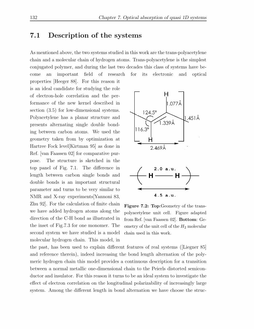
132 Chapter 7. Optical absorption of quasi 1D systems
7.1 Description of the systems
As mentioned above, the two systems studied in this work are the trans-polyacetylene
chain and a molecular chain of hydrogen atoms. Trans-polyacetylene is the simplest
conjugated polymer, and during the last two decades this class of systems have be-
come an important field of research for its electronic and optical
H H2.0 a.u.
4.5 a.u.
Figure 7.2: Top:Geometry of the trans-
polyacetylene unit cell. Figure adapted
from Ref. [van Faassen 02]. Bottom: Ge-
ometry of the unit cell of the H2 molecular
chain used in this work.
properties [Heeger 88]. For this reason it
is an ideal candidate for studying the role
of electron-hole correlation and the per-
formance of the new kernel described in
section (3.5) for low-dimensional systems.
Polyacetylene has a planar structure and
presents alternating single double bond-
ing between carbon atoms. We used the
geometry taken from by optimization at
Hartree Fock level[Kirtman 95] as done in
Ref. [van Faassen 02] for comparative pur-
pose. The structure is sketched in the
top panel of Fig. 7.1. The difference in
length between carbon single bonds and
double bonds is an important structural
parameter and turns to be very similar to
NMR and X-ray experiments[Yannoni 83,
Zhu 92]. For the calculation of finite chain
we have added hydrogen atoms along the
direction of the C-H bond as illustrated in
the inset of Fig.7.3 for one monomer. The
second system we have studied is a model
molecular hydrogen chain. This model, in
the past, has been used to explain different features of real systems ([Liegner 85]
and reference therein), indeed increasing the bond length alternation of the poly-
meric hydrogen chain this model provides a continuous description for a transition
between a normal metallic one-dimensional chain to the Peierls distorted semicon-
ductor and insulator. For this reason it turns to be an ideal system to investigate the
effect of electron correlation on the longitudinal polarizability of increasingly large
system. Among the different length in bond alternation we have choose the struc-

7.2 One Monomer spectra 133
ture sketched in the bottom panel of Fig. 7.1. The hydrogen atoms have an intra-
molecular distance of 2 a.u. and the inter-molecular distance between H2 molecules
is 2.5 a.u.. Sanchez et al. [Sanchez 03] showed that this is the geometry where the
LDA polarizability has the maximum error with respect the Hartree Fock calcu-
lation for two interacting H2 molecules 2 , so it constitutes a stringent test case
for the new f(1)xc introduced in section (3.5). In all the calculation the position
of the atoms are kept fixed. The ground state wave functions and eigen-energies
of all the studied systems have been performed with the plane wave ABINIT code
in DFT framework using the LDA approximation in the Teter Pade parametriza-
tion [Goedecker 96], if not differently specified. The electron-ion interaction has
been considered via Troulliers-Martin pseudopotentials [Troullier 91]. The optical
properties have been calculated with the code SELF as described in section (4.3).
The longitudinal polarizability per monomer of this model with different bond al-
ternation has been studied with different techniques and approximations as coupled
and unrestricted Hartree Fock , Møller Plesset [Champagne 95a, Champagne 95b],
DFT [van Faassen 02, Sanchez 03, Kummel 04, Baer 05], and quantum Monte-
carlo [Umari 05].
7.2 One Monomer spectra
The first systems we have considered are single oligomers of the atomic chains: an
isolate monomer of polyacetylene and an H2 molecule (look insets in Fig 7.3). For
these small systems we have compared the TDDFT results when the new non-local
and energy dependent kernel described in section (3.5) is used, with the absorption
spectra obtained solving the BS equation of MBPT. The results in different approx-
imations are shown in Fig. 7.3. For both molecules we have used a cubic supercell
of side length of 25 a.u. for H2 and 33 a.u. for the polyacetylene monomer. To
avoid the spurious interaction of the supercell images we have used a cutoff coulomb
potential of spherical shape Eq. (5.11). The first step for both BS and TDDFT
calculation is the evaluation of the quasiparticle energies that has been calculated
2 This paper they attributes the failure of the LDA to the self-interaction error: for small inter-
molecular distances, as a covalent bond, the system does not have fractional number of electrons,
therefore the error is small, when the inter-molecular distance increase the applied electric field
produces charge transfer and the error increases, then for larger inter-molecular distances the
system approach two independent H2 molecules, the charge transfer decreases and consequently
the LDA error.
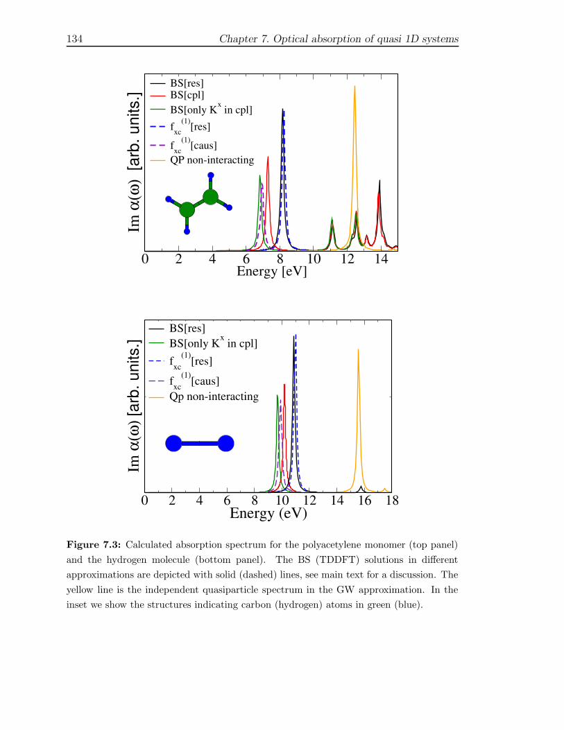
134 Chapter 7. Optical absorption of quasi 1D systems
0 2 4 6 8 10 12 14Energy [eV]
Im α
(ω)
[arb
. uni
ts.]
BS[res]BS[cpl]BS[only Kx in cpl]fxc
(1)[res]fxc
(1)[caus]QP non-interacting
0 2 4 6 8 10 12 14 16 18Energy (eV)
Im α
(ω) [
arb.
uni
ts.]
BS[res]BS[only Kx in cpl]fxc
(1)[res]fxc
(1)[caus]Qp non-interacting
Figure 7.3: Calculated absorption spectrum for the polyacetylene monomer (top panel)
and the hydrogen molecule (bottom panel). The BS (TDDFT) solutions in different
approximations are depicted with solid (dashed) lines, see main text for a discussion. The
yellow line is the independent quasiparticle spectrum in the GW approximation. In the
inset we show the structures indicating carbon (hydrogen) atoms in green (blue).
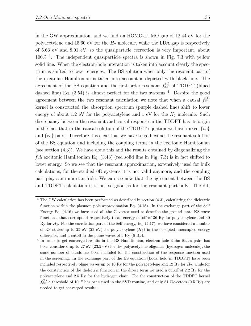
7.2 One Monomer spectra 135
in the GW approximation, and we find an HOMO-LUMO gap of 12.44 eV for the
polyacetylene and 15.60 eV for the H2 molecule, while the LDA gap is respectively
of 5.63 eV and 8.01 eV, so the quasiparticle correction is very important, about
100% 3. The independent quasiparticle spectra is shown in Fig. 7.3 with yellow
solid line. When the electron-hole interaction is taken into account clearly the spec-
trum is shifted to lower energies. The BS solution when only the resonant part of
the excitonic Hamiltonian is taken into account is depicted with black line. The
agreement of the BS equation and the first order resonant f(1)xc of TDDFT (blued
dashed line) Eq. (3.54) is almost perfect for the two systems 4. Despite the good
agreement between the two resonant calculation we note that when a causal f(1)xc
kernel is constructed the absorption spectrum (purple dashed line) shift to lower
energy of about 1.2 eV for the polyacetylene and 1 eV for the H2 molecule. Such
discrepancy between the resonant and causal response in the TDDFT has its origin
in the fact that in the causal solution of the TDDFT equation we have mixed vcand cv pairs. Therefore it is clear that we have to go beyond the resonant solution
of the BS equation and including the coupling terms in the excitonic Hamiltonian
(see section (4.3)). We have done this and the results obtained by diagonalizing the
full excitonic Hamiltonian Eq. (3.43) (red solid line in Fig. 7.3) is in fact shifted to
lower energy. So we see that the resonant approximation, extensively used for bulk
calculations, for the studied 0D systems it is not valid anymore, and the coupling
part plays an important role. We can see now that the agreement between the BS
and TDDFT calculation it is not so good as for the resonant part only. The dif-
3 The GW calculation has been performed as described in section (4.3), calculating the dielectric
function within the plasmon pole approximation Eq. (4.18). In the exchange part of the Self
Energy Eq. (4.16) we have used all the G vector used to describe the ground state KS wave
functions, that correspond respectively to an energy cutoff of 36 Ry for polyacetylene and 40
Ry for H2. For the correlation part of the Self-energy, Eq. (4.17), we have considered a number
of KS states up to 25 eV (23 eV) for polyacetylene (H2) in the occupied-unoccupied energy
difference, and a cutoff in the plane waves of 5 Ry (6 Ry).4 In order to get converged results in the BS Hamiltonian, electron-hole Kohn Sham pairs has
been considered up to 27 eV (23.5 eV) for the polyacetylene oligomer (hydrogen molecule), the
same number of bands has been included for the construction of the response function used
in the screening. In the exchange part of the BS equation (Local field in TDDFT) have been
included respectively plane waves up to 10 Ry for the polyacetylene and 12 Ry for H2, while for
the construction of the dielectric function in the direct term we used a cutoff of 2.2 Ry for the
polyacetylene and 2.5 Ry for the hydrogen chain. For the construction of the TDDFT kernel
f(1)xc a threshold of 10−9 has been used in the SVD routine, and only 81 G-vectors (0.5 Ry) are
needed to get converged results.
136 Chapter 7. Optical absorption of quasi 1D systems
ference between the two absorption spectra is due to the contribution of the direct
term in the coupling part. This can be seen from the fact that the f(1)xc kernel is
constructed starting from the only resonant part of the kernel of the BS equation,
and while the exchange part of the coupling is recovered in the TDDFT equation
when causal response function are considered, including the local field effects, the
direct part in the coupling is neglected. This is shown in the spectra plotted in green
in Figure 7.3 labeled [only Kx in cpl] where we have diagonalized the BS equation
including the resonant part of Eq. (3.44), and only the exchange part in the coupling
Eq. (3.46). In this case agreement is restored. Anyway, fortunately the contributions
that are included in the f(1)xc (the direct term in the coupling part) plays a minor
role. The overall difference between the full BS equation and the TDDFT causal
calculation is about 0.2 eV. For the sake of clarity we have not reproduced in the
top of Fig. 7.3 the ALDA spectrum, showed before in Fig. 5.10, but as expected for
finite systems, in the case of just one isolate molecule, also the ALDA reproduce
well the absorption spectrum (compared to the BS result). In conclusion, we have
shown that TDDFT with a first order f(1)xc , that were previously tested for bulk and
surface systems [Marini 03, Sottile 03, Pulci 06] , reproduces fairly well the optical
properties of isolated 0D systems. Minor discrepancies are found due to the ab-
sence of the contribution coming from the direct term in the coupling part of the BS
Hamiltonian in the kernel, that in some cases can play a role. Anyway, as we will see
in the next section, the contribution of the coupling part in the absorption spectrum
get smaller as the length of the polymeric chain is increased, and consequently the
discrepancies observed here tends to disappear in the long chain limit, where the
ALDA fails for the reason illustrated in the introduction.
7.3 Optical properties of finite chains
In the last section we have seen the performance of the new kernel f(1)xc at first order
when applied for studying small isolated molecules and we have found satisfactory
results when compared with the ALDA calculation and Bethe Salpeter calculation.
Now in this section we study the optical properties of the trans-polyacetylene poly-
mer and the H2n chain in function of the length of the chain5. As stated in the
5 For all these calculation, apart for the single monomer where we have used cubic supercells, we
have used parallelepiped supercells with sides of 25a.u. in the directions orthogonal to the chain
axis for the hydrogen and 30a.u. for the polyacetylene. In order to avoid spurious interactionsbetween cells we have used the cutoff coulomb interaction described in chapter (5) with a cylin-
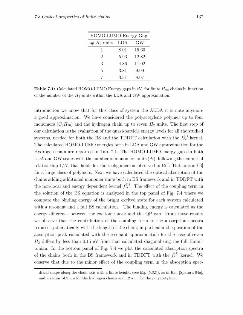
7.3 Optical properties of finite chains 137
HOMO-LUMO Energy Gap
# H2 units LDA GW
1 8.01 15.60
2 5.93 12.82
3 4.86 11.02
5 3.81 9.09
7 3.31 8.07
Table 7.1: Calculated HOMO-LUMO Energy gaps in eV, for finite H2n chains in function
of the number of the H2 units within the LDA and GW approximation.
introduction we know that for this class of system the ALDA it is note anymore
a good approximation. We have considered the polyacetylene polymer up to four
monomers (C8H16) and the hydrogen chain up to seven H2 units. The first step of
our calculation is the evaluation of the quasi-particle energy levels for all the studied
systems, needed for both the BS and the TDDFT calculation with the f(1)xc kernel.
The calculated HOMO-LUMO energies both in LDA and GW approximation for the
Hydrogen chain are reported in Tab. 7.1. The HOMO-LUMO energy gaps in both
LDA and GW scales with the number of monomers units (N), following the empirical
relationship 1/N , that holds for short oligomers as observed in Ref. [Hutchinson 03]
for a large class of polymers. Next we have calculated the optical absorption of the
chains adding additional monomer units both in BS framework and in TDDFT with
the non-local and energy dependent kernel f(1)xc . The effect of the coupling term in
the solution of the BS equation is analyzed in the top panel of Fig. 7.4 where we
compare the binding energy of the bright excited state for each system calculated
with a resonant and a full BS calculation. The binding energy is calculated as the
energy difference between the excitonic peak and the QP gap. From those results
we observe that the contribution of the coupling term to the absorption spectra
reduces systematically with the length of the chain, in particular the position of the
absorption peak calculated with the resonant approximation for the case of seven
H2 differs by less than 0.15 eV from that calculated diagonalizing the full Hamil-
tonian. In the bottom panel of Fig. 7.4 we plot the calculated absorption spectra
of the chains both in the BS framework and in TDDFT with the f(1)xc kernel. We
observe that due to the minor effect of the coupling term in the absorption spec-
drical shape along the chain axis with a finite height, (see Eq. (5.32)), as in Ref. [Spataru 04a],
and a radius of 9 a.u for the hydrogen chains and 12 a.u. for the polyacetylene.
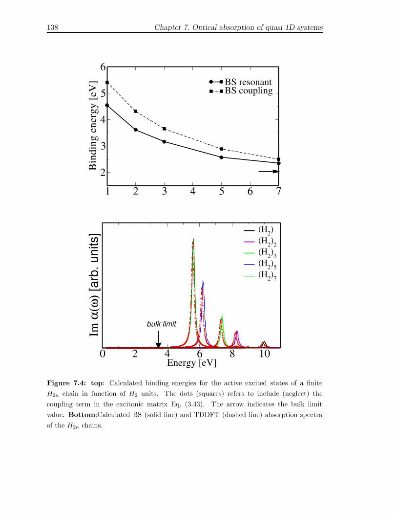
138 Chapter 7. Optical absorption of quasi 1D systems
1 2 3 4 5 6 7Number of H2 units
2
3
4
5
6
Bind
ing
ener
gy [e
V] BS resonant
BS coupling
0 2 4 6 8 10Energy [eV]
Im α
(ω) [
arb.
uni
ts] (H2)
(H2)2(H2)3(H2)5(H2)7
bulk limit
Figure 7.4: top: Calculated binding energies for the active excited states of a finite
H2n chain in function of H2 units. The dots (squares) refers to include (neglect) the
coupling term in the excitonic matrix Eq. (3.43). The arrow indicates the bulk limit
value. Bottom:Calculated BS (solid line) and TDDFT (dashed line) absorption spectra
of the H2n chains.

7.3 Optical properties of finite chains 139
1 2 3 4 5 6 7Number of monomers
0
2
4
6
8
10
12
Ener
gy [e
V]
Bulk limit
Figure 7.5: Excitation energies for the singlet and triplet excited states of the chains.
With bullets (triangles) we indicate the singlet (triplet) excitations. In red (blue) are
indicated the singlet (triplet) excitations with oscillator strength different from zero. w
trum, the agreement between the two calculation improves with chain length, and for
the larger chains studied here the results obtained with the two methods are quite
indistinguishable. In Figure. 7.5 are plotted the whole excitation energies of the
optically active singlet states (bullets) in function of the number of monomers units
up to 13 eV, together with the triplet excited states obtained by diagonalization of
HOMO-LUMO Energy Gap
# monomer units LDA GW
1 5.63 12.44
2 3.94 9.55
3 3.11 7.94
4 2.44 6.84
Table 7.2: Calculated HOMO-LUMO Energy gaps in
eV, for finite trans-polyacetylene chains in function of
(C2H4) units within the LDA and GW approximation.
Eq. (3.47) (triangles). The
bright excitations are indicated
with colored symbols , while
in black we indicate the ex-
citations with zero or very
small oscillator strength. The
same study has been made for
the polyacetylene chain up to
four monomer. The calculated
LDA and GW HOMO-LUMO
gap energies are reported in
Tab. 7.2, and the 1/N behavior
encountered for the H2n chain
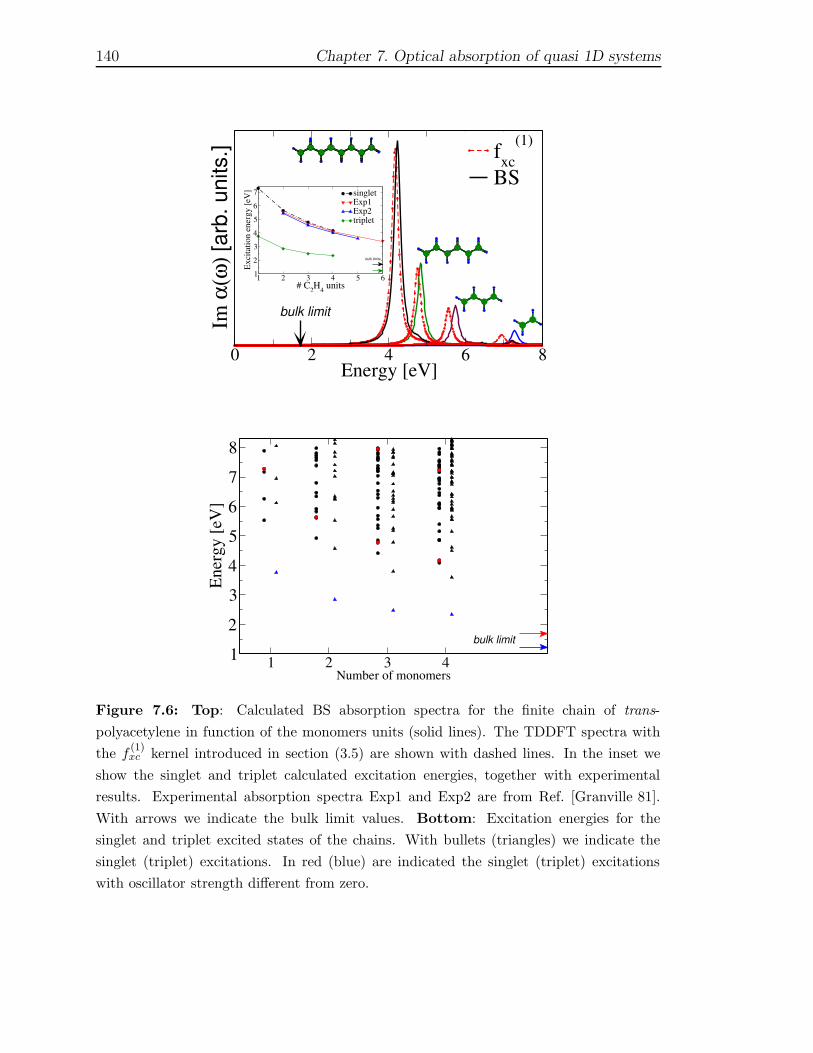
140 Chapter 7. Optical absorption of quasi 1D systems
0 2 4 6 8Energy [eV]
Im α
(ω) [
arb.
uni
ts.] fxc
(1)
BS
bulk limit
1 2 3 4 5 6# C2H4 units
1
2
3
4
5
6
7
Exci
tatio
n en
ergy
[eV
] singletExp1Exp2triplet
bulk limits
1 2 3 4Number of monomers
12345678
Ener
gy [e
V]
bulk limit
Figure 7.6: Top: Calculated BS absorption spectra for the finite chain of trans-
polyacetylene in function of the monomers units (solid lines). The TDDFT spectra with
the f(1)xc kernel introduced in section (3.5) are shown with dashed lines. In the inset we
show the singlet and triplet calculated excitation energies, together with experimental
results. Experimental absorption spectra Exp1 and Exp2 are from Ref. [Granville 81].
With arrows we indicate the bulk limit values. Bottom: Excitation energies for the
singlet and triplet excited states of the chains. With bullets (triangles) we indicate the
singlet (triplet) excitations. In red (blue) are indicated the singlet (triplet) excitations
with oscillator strength different from zero.
7.3 Optical properties of finite chains 141
is also obtained for the polyacetylene chain. The calculated absorption spectra are
plotted in Fig. 7.6. The agreement between the BS and TDDFT calculations is
worse than in the case of the hydrogen chains for the single oligomer and for the
two monomers chain, but as in the case of the hydrogen chain we found that the
agreement improves for larger chains, when the coupling contribution to the spectra
can be neglected. For the three and four units chain we found a quite perfect agree-
ment between the BS calculation and the TDDFT calculation. In the inset of the
same figure we plot the singlet and triplet excitation energies. The singlet excita-
tion are compared with two experiments taken from Ref. [Granville 81]. These two
experimental data, labeled [exp1] and [exp2] corresponds to absorption experiments
at two different temperatures, 293 K and 77 K respectively. We find a very good
agreement between calculated and experimental excitation energies, even if care has
to be taken in the comparison because our calculations are performed on idealized
structures with a fixed alternating bonding independent on the chain length. The
whole set of excitation energies for both singlet and triplet states up to 8.3 eV is
plotted in the bottom part of Fig.7.6. We see that, at difference of the hydrogen
chain, the first bright state lies above dark states. As we will see later this is not
the case for the infinite polymer where the first excitation is bright. From our calcu-
lations we can observe that the energy difference between the “bright” and “dark”
states reduces adding monomers, and in the bigger chain (four monomer) the bright
and the dark states have quite the same energies, but the crossover take place for
chains longer than the ones we have studied until now.
In conclusion the new first order kernel works very well also for describing the
absorption spectra of finite systems, giving an overall agreement with the BS calcu-
lations. Minor differences are encountered for the smaller systems we have studied.
These differences can be ascribed to the effect of the direct term of the coupling
part of the BS equation that is not included in the construction of the kernel.
Next we have calculated in TDDFT the statical axial polarizability for these
finite systems both in ALDA and with the new kernel. The axial polarizability is
obtained from Eq. (5.29) The results are shown in Fig. 7.7 and 7.8, where the axial
polarizability for monomer is plotted in function of the monomer units, and they
are compared with previous Hartree Fock and Vignale Kohn calculations present in
the literature (see caption). For both systems we find that the f(1)xc kernel, due to its
non-locality gives a huge correction to the ALDA, bringing the results close to the
more accurate quantum chemistry calculation. Concerning the polyacetylene chain
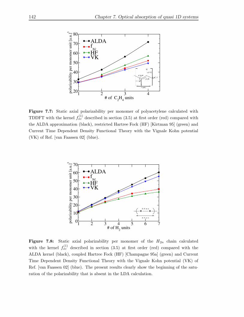
142 Chapter 7. Optical absorption of quasi 1D systems
1 2 3 4# of C2H4 units
20
30
40
50
60
70
80
pola
rizab
ility
per
mon
omer
uni
t [a.
u.]3
ALDAfxcHFVK
Figure 7.7: Static axial polarizability per monomer of polyacetylene calculated with
TDDFT with the kernel f(1)xc described in section (3.5) at first order (red) compared with
the ALDA approximation (black), restricted Hartree Fock (HF) [Kirtman 95] (green) and
Current Time Dependent Density Functional Theory with the Vignale Kohn potential
(VK) of Ref. [van Faassen 02] (blue).
1 2 3 4 5 6 7# of H2 units
0
10
20
30
40
50
60
70
pola
rizab
ility
per
mon
omer
uni
t [a.
u.]3
ALDAfxcHFVK
H H2.0 a.u.
4.5 a.u.
Figure 7.8: Static axial polarizability per monomer of the H2n chain calculated
with the kernel f(1)xc described in section (3.5) at first order (red) compared with the
ALDA kernel (black), coupled Hartree Fock (HF) [Champagne 95a] (green) and Current
Time Dependent Density Functional Theory with the Vignale Kohn potential (VK) of
Ref. [van Faassen 02] (blue). The present results clearly show the beginning of the satu-
ration of the polarizability that is absent in the LDA calculation.
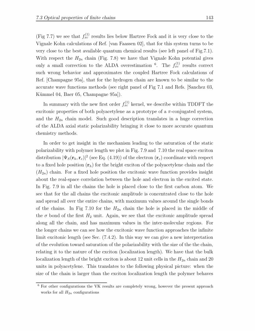
7.3 Optical properties of finite chains 143
(Fig 7.7) we see that f(1)xc results lies below Hartree Fock and it is very close to the
Vignale Kohn calculations of Ref. [van Faassen 02], that for this system turns to be
very close to the best available quantum chemical results (see left panel of Fig.7.1).
With respect the H2n chain (Fig. 7.8) we have that Vignale Kohn potential gives
only a small correction to the ALDA overestimation 6. The f(1)xc results correct
such wrong behavior and approximates the coupled Hartree Fock calculations of
Ref. [Champagne 95a], that for the hydrogen chain are known to be similar to the
accurate wave functions methods (see right panel of Fig 7.1 and Refs. [Sanchez 03,
Kummel 04, Baer 05, Champagne 95a]).
In summary with the new first order f(1)xc kernel, we describe within TDDFT the
excitonic properties of both polyacetylene as a prototype of a π-conjugated system,
and the H2n chain model. Such good description translates in a huge correction
of the ALDA axial static polarizability bringing it close to more accurate quantum
chemistry methods.
In order to get insight in the mechanism leading to the saturation of the static
polarizability with polymer length we plot in Fig. 7.9 and 7.10 the real space exciton
distribution |ΨS(rh, re)|2 (see Eq. (4.19)) of the electron (re) coordinate with respect
to a fixed hole position (rh) for the bright exciton of the polyacetylene chain and the
(H2n) chain. For a fixed hole position the excitonic wave function provides insight
about the real-space correlation between the hole and electron in the excited state.
In Fig. 7.9 in all the chains the hole is placed close to the first carbon atom. We
see that for the all chains the excitonic amplitude is concentrated close to the hole
and spread all over the entire chains, with maximum values around the single bonds
of the chains. In Fig 7.10 for the H2n chain the hole is placed in the middle of
the σ bond of the first H2 unit. Again, we see that the excitonic amplitude spread
along all the chain, and has maximum values in the inter-molecular regions. For
the longer chains we can see how the excitonic wave function approaches the infinite
limit excitonic length (see Sec. (7.4.2). In this way we can give a new interpretation
of the evolution toward saturation of the polarizability with the size of the the chain,
relating it to the nature of the exciton (localization length). We have that the bulk
localization length of the bright exciton is about 12 unit cells in the H2n chain and 20
units in polyacetylene. This translates to the following physical picture: when the
size of the chain is larger than the exciton localization length the polymer behaves
6 For other configurations the VK results are completely wrong, however the present approach
works for all H2n configurations
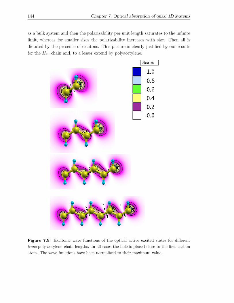
144 Chapter 7. Optical absorption of quasi 1D systems
as a bulk system and then the polarizability per unit length saturates to the infinite
limit, whereas for smaller sizes the polarizability increases with size. Then all is
dictated by the presence of excitons. This picture is clearly justified by our results
for the H2n chain and, to a lesser extend by polyacetylene.
Figure 7.9: Excitonic wave functions of the optical active excited states for different
trans-polyacetylene chain lengths. In all cases the hole is placed close to the first carbon
atom. The wave functions have been normalized to their maximum value.

7.3 Optical properties of finite chains 145
Figure 7.10: Excitonic wave functions of the optical active excited states for different
H2n chain lengths up to n=7. In all cases the hole is placed in the middle of the bond of
the first H2 units. The wave functions have been normalized to their maximum value.
146 Chapter 7. Optical absorption of quasi 1D systems
7.4 Infinite chains
In this section we look at more in detail to the periodic, infinite, chain both for H2n
and polyacetylene.
7.4.1 Trans-Polyacetylene
The structure of the polyacetylene polymer has just been sketched in Fig. 7.1, to-
gether with the lattice constant in the direction of the polymer axis. The calculated
LDA band gap is of 0.78 eV, whereas the GW calculation opens it to 2.13 eV 7. The
band structure along the Γ −X direction both in LDA and GW approximations is
showed in Fig. 7.11, adjusted by placing the Fermi energy at 0 eV. The LDA and
GW band structures exhibit similar dispersion, being the main difference the open-
ing of the bans gap (scissor operator). We note that as showed in chapter (5) for
the H2n chain, the modified cutoff potential speeds up the convergence of the band
gap energy with respect to the empty space in the supercell, that is very slow when
the bare coulomb potential is used (see top panel of Fig. 7.11). When the cutoff
potential is used, we see that a side of 33 a.u. in the directions orthogonal to the
chain axis is enough to get a converged band gap value. To obtain a converged GW
band structure we have used a one-dimensional grid of 61 k points in the direction
of the polymer axis. To calculate the screening we introduce bands up to 35 eV
in the electron-hole KS states and a plane wave cutoff of 12 Ry. The converged
value of the fundamental direct gap at the X point (2.13 eV), it is very closed to the
value reported in Ref. [Rohlfing 99] (2.1 eV) calculated with a localized base code,
so without any problem of spurious images interactions. The absorption spectra
calculated in the BS framework and in TDDFT with the f(1)xc kernel are plotted in
Fig. 7.12. In the same figure we also plot a TDDFT spectrum calculated with the
ALDA and the independent quasi particle spectrum, i.e. the spectrum neglecting
the electron-hole interaction. Those spectra were calculated considering light with
electric field polarization vector parallel to the chain. First we note that in the case
of the infinite polymer the coupling term in the excitonic Hamiltonian has no effect
in the optical absorption spectrum, so here the resonant approximation for the BS
equation is totally justified. Next we see that for this system the agreement of the
7 The ground state LDA eigenfunctions and eigenvalues have been obtained using a plane wave
energy cutoff of 36 Ry., we have truncated the coulomb potential using the method described
in chapter 5, using a supercell of size 4.643x33x33 a.u. and a cutoff radius of 12 a.u..

7.4 Infinite chains 147
2000 4000 6000 8000 10000Supercell Volume [a.u.]3
1.5
2
2.5
Qua
sipar
ticle
ene
rgy
gap
[eV
] 23 33 38 41 44Interchain distance [a.u.]
Bare coulomb Modified coulomb potential
Γ X-20
-16
-12
-8
-4
0
4
8
Ener
gy (e
V)
LDA
Γ X-20
-16
-12
-8
-4
0
4
8
Ener
gy (e
V)
GW
Figure 7.11: Top: Calculated band gap at X point of trans polyacetylene in GW ap-
proximation for different supercell size with bare coulomb and modified coulomb potential
described in chapter 5. Calculated band structures of trans polyacetylene along the chain
axis in LDA approximation (middle panel) and GW approximation (bottom panel). In
both cases, the zero corresponds to the Fermi level.

148 Chapter 7. Optical absorption of quasi 1D systems
0 1 2 3 4Energy [eV]
Im α
(ω) [
arb.
uni
ts.]
BSQP fxc
(1)
ALDA
1.7 eVexp. peak
Figure 7.12: Calculated absorption spectrum for the polyacetylene polymer in BS frame-
work and in TDDFT with the f(1)xc kernel, compared with the ALDA calculation and the
non interacting quasi-particle spectrum.
TDDFT calculation with the kernel f(1)xc (blue line) is practically indistinguishable
from the Bethe Salpeter calculation (black line) and presents a single sharp peak
placed at 1.69 eV. Above 2 eV the system is nearly transparent. Such result is in
good agreement with the measured spectrum which has maximum absorption at 1.7
eV [Leising 88] and with the previous BS result of Ref. [Rohlfing 99]. Clearly we see
that the ALDA spectrum totally fails in the description of the optical absorption
of this quasi 1-dimensional system as it does for other insulators (bulk or surfaces).
Beyond the bright exciton at 1.69 eV that we now indicate with Sb, another bound
exciton is found at 1.86 eV with piratically zero oscillator strength that we indicate
with Sd. Both excitons arise mainly from π → π∗ transitions, the spectrum results
to be converged including only few bands in the excitonic matrix (we used two va-
lence bands and two conduction bands), and only electron-hole states close to the
X point contribute to the formation of the excitons, as just previously observed in
Ref. [Rohlfing 99] 8. With respect the triplet excitations, that cannot be excited by
8 Here we stress that, as previously stated in chapter( 5), the one dimensional sampling of the
Brillouin zone is allowed thanks to the use of the cutoff coulomb potential, whereas for calcu-
lations with the bare coulomb potential a three dimensional sampling is needed in order to get
converged results. The plane wave cutoff for the exchange and direct terms of the excitonic

7.4 Infinite chains 149
Trans Polyacetylene This work [Rohlfing 99] [Rohlfing 04] [Puschnig 03]
Singlet Sb 0.44 0.4 0.5 0.6
Sd 0.27 0.3 0.38
Triplet T1 0.91 1.2 0.99 1.3
T2 0.31 0.4 0.43
Table 7.3: Calculated binding energies in eV of the singlet and triplet excited states of
the trans-polyacetylene, compared with the results of previous Bethe Salpeter calculations
with different implementations.
PRQTS UWVYX[Z Z \]X^V_S U `[aPRQTS UWVYX[Z Z \bU cTX^V_S U `da
e[f gihkj lklnmpo qe[f gihkj rYsWmpo q
-80 -60 -40 -20 0 20 40 60 80Distance from the hole [A]
Elec
tron
distr
ibut
ion
-30 -20 -10 0 10 20 30Distance form the hole in [C2H2] units
Optically active
Optically inactive
Figure 7.13: Electron-hole wave functions of the “bright” (1.69 eV) and “dark” (1.93
eV) excitons of the polyacetylene, showing the distribution of the electron relative to the
hole fixed at 0A. In the top part the excitonic wave function is plotted in the plane where
the polymer lie, while in the bottom panel it is averaged in a plane perpendicular to the
chain: ΨS(xe, r0h) =
∫
dr⊥e ΨS(re, r0h). With an arrow we have indicated the position of the
hole.
Hamiltonian is respectively of 6.8 Ry and 5.8 Ry.
150 Chapter 7. Optical absorption of quasi 1D systems
light, we again found two bound excitons, placed at 1.22 eV and 1.82 eV. The bind-
ing energies of the singlet and triplet bound excitons found in the present calculation
are summarized in Tab. 7.3, together with others Bethe Salpeter calculations. The
electron-hole wave functions in real space of the two singlet bound excitons states
are depicted in Fig. 7.13. The hole is fixed in an arbitrary position on the polymer
chain and is placed in the center of the panels. We see that the first optically active
exciton is very extended in space, having a size of about 50A, and spreading about
20 unit cells. The second optically inactive excitons is even more extended. The
polarizability per monomer unit has been calculated in the same way we did for the
finite chains, i.e. in reciprocal space for the new kernel and in configuration space
for the ALDA. The polarizability values are 971.2 a.u. in ALDA approximation and
537.19 a.u. with the f(1)xc kernel. Thus, we obtain a huge reduction of the polariz-
ability when the new kernel is used with respect the ALDA value in agreement with
the trends found for finite systems.
7.4.2 Hydrogen chain
The same study made for the polyacetylene has been performed for the infinite
(H2n) chain. The structure of the chain has been described in the introduction of
this chapter. We have used a supercell of size 4.5×25×25 a.u., and a cutoff radius of
8 a.u. for the cylindrical cutoff coulomb potential. The ground state wave functions
have been obtained with a plane wave energy cutoff of 40 Ry. The quasiparticle
band structure along the Γ-X direction in the GW approximation is presented in
Fig. 7.14 together with the result. The calculated LDA gap at the X point of the
one-dimensional Brillouin zone is 2.28 eV, whereas the GW calculation yield a band
gap of 5.49 eV. In order to obtain converged quasiparticle energies we have adopted
a one dimensional sampling of the Brillouin zone using 61 k points. The exchange
part of the self energy, Eq. (4.16), has been calculated using the same plane wave
cutoff used in the computation of the wave functions, while for the correlation part,
Eq. (4.17) we have used bands up to 25 eV and a plane wave cutoff of 8 Ry. As in the
case of the polyacetylene the LDA and GW band structures are qualitatively similar,
and the main change is the gap opening that in the GW is nearly twice the LDA
one. Thanks to this we can take in account the GW correction trough a scissor
operator for the BS calculation and for building f(1)xc in TDDFT. The calculated
absorption spectra in different approximation is showed in Fig. 7.15. As in the
case of the trans-polyacetylene polymer we observe that the coupling terms can

7.4 Infinite chains 151
Γ X
-5
0
5
10
15
Ener
gy (e
V)
LDA
Γ X
-5
0
5
10
15
20
Ener
gy (e
V)
GW
Figure 7.14: Calculated band structure of the H2n chain in the Γ−X direction in LDA
(top panel) and GW approximation (bottom panel). In both figure the zero of energy is
placed at the Fermi level.
be neglected in the excitonic Hamiltonian and we can consider only the resonant
part. The BS spectrum is showed with a black solid line. When compared with
the non-interacting quasiparticle spectra (green line) we observe that the hydrogen
chain presents a bound exciton having a large binding energy of 2.03 eV. With
respect the TDDFT calculation we see that the f(1)xc reproduces perfectly the BS
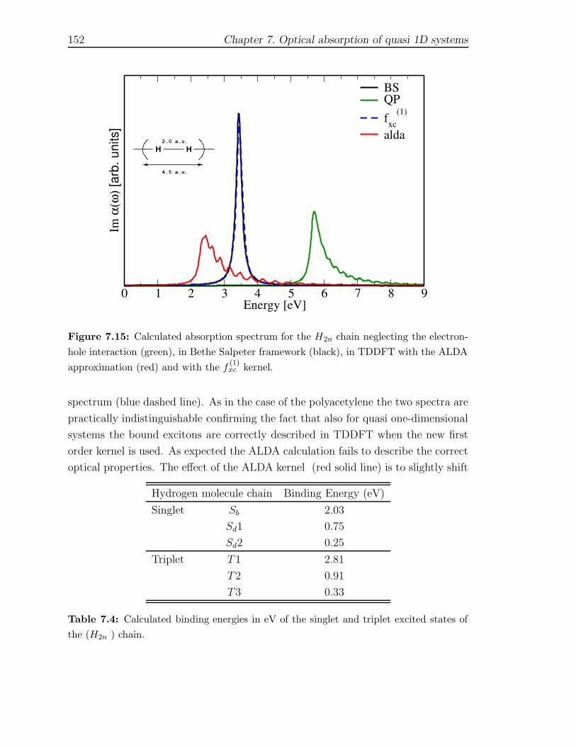
152 Chapter 7. Optical absorption of quasi 1D systems
0 1 2 3 4 5 6 7 8 9Energy [eV]
Im α
(ω) [
arb.
uni
ts]
BSQP fxc
(1)
aldaH H2.0 a.u.
4.5 a.u.
Figure 7.15: Calculated absorption spectrum for the H2n chain neglecting the electron-
hole interaction (green), in Bethe Salpeter framework (black), in TDDFT with the ALDA
approximation (red) and with the f(1)xc kernel.
spectrum (blue dashed line). As in the case of the polyacetylene the two spectra are
practically indistinguishable confirming the fact that also for quasi one-dimensional
systems the bound excitons are correctly described in TDDFT when the new first
order kernel is used. As expected the ALDA calculation fails to describe the correct
optical properties. The effect of the ALDA kernel (red solid line) is to slightly shift
Hydrogen molecule chain Binding Energy (eV)
Singlet Sb 2.03
Sd1 0.75
Sd2 0.25
Triplet T1 2.81
T2 0.91
T3 0.33
Table 7.4: Calculated binding energies in eV of the singlet and triplet excited states of
the (H2n ) chain.

7.4 Infinite chains 153
00
0.02
0.04-20 -10 0 10 20 30-30
Distance from the hole [H2] units
0
0.01
0.02
Elec
tron
distr
ibut
ion
-80 -60 -40 -20 0 20 40 60 80Distance from the Hole [A]
0
0.01
Active 3.45 eV
Inactive 4.73 eV
Inactive 5.23 eV
Figure 7.16: Excitonic wave functions of the bound excitons of the H2n chain along the
chain axis averaged in a plane perpendicular to the polymer. The hole in fixed in the
center of the panel and it is placed in the middle of the H2 bond.
the non interacting Kohn-Sham spectra at higher energies. In Fig. 7.15 the non
interacting Kohn-Sham absorption spectra it is not depicted for reason of clarity,
but it is essentially the non interacting QP spectra (green slide line) shifted by 3.21
eV (the scissor operator) to lower energies. Above the bright excitons placed at
3.46 eV we find other two ’dark’ excited states (at 4.74 eV and 5.24 eV) below the
quasiparticle gap placed. The binding energies of the bright and darks excitons are
summarized in Table. 7.4 together with the corresponding triplet excited states. The
triplet excitations binding energies are larger since the repulsive exchange interaction
between the electron and hole is absent for spin-triplet excitations. The electron-hole
wave functions for the singlet excited states are showed in Fig. 7.16. In the three
plots the hole is fixed in 0 and it is in the middle of the H2 bond. We can see that the
electron distribution with respect the hole position is more localized than in the case
of the polyacetylene, extending over about 40 A(20 oligomer units). The excitonic
wave functions of the higher lying “dark states” are more extended in space. The
calculated axial polarizability in TDDFT with the ALDA and the f(1)xc kernel are

154 Chapter 7. Optical absorption of quasi 1D systems
respectively 160.9 a.u. and 120.6 a.u.. Berger et al. [Berger 05] found 162.28 a.u.
in ALDA approximation and 131.28 a.u. with the Vignale Kohn functional. We
see that the non local kernel partially correct the overestimation of the ALDA and
gives a better results than the Vignale-Kohn functional even if the calculated value
it is still consistently bigger than the Quantum Monte Carlo calculation which is
53.4 ± 1.1a.u..
Role of the ground state wave functions
Until now we have shown how the ALDA fails in the calculation of optical proper-
ties of linear chains and how a better description can be achieved either resorting
to the Many Body Perturbation Theory via the Bethe-Salpeter equation or using
more elaborated non-local kernels that mimics the MBPT results. As described in
the introduction, the solution of the BS equation requires as starting ingredient, the
ground state wave functions for both occupied and unoccupied states that until now
have been calculated within Density Functional Theory in the LDA approximation.
In this section we want to quantify the role of the initial wave functions in the
calculation of the Bethe-Salpeter absorption spectra 9. We have repeated the calcu-
lation of the absorption spectra in BS framework showed in Fig. 7.15 but instead of
using LDA ground state wave-functions we have used exact exchange ground state
wave function in the KLI approximation as described in section (1.27). The DFT
band gap calculated with these wave functions is 3.0 eV and we have skipped the
calculation of the quasi-particle band structure and we adjusted the scissor oper-
ator for the KLI calculation in order to have the same quasiparticle band gap of
the LDA+GW calculation. In Fig. 7.17 we compare the obtained interacting and
non-interacting spectra with the previous calculation made with the LDA wave-
functions. The two non-interacting quasiparticle spectra have the same onset by
construction. When the electron-hole interaction is considered we see that the use
of the KLI wave functions give rise to a bound exciton with a larger binding energy
than the LDA+BSE calculation. We have also performed using both LDA and KLI
ground state wave-functions a calculation considering the exchange part only in the
excitonic Hamiltonian, that is equivalent to the RPA approximation. No differences
have been observed between the two calculations, so the observed difference has to
be addressed to the direct term, thus the quality of the ground state wave-functions
9 Here we do not investigate the impact on the quasi particle energies in the GW approximation,
that will require a deeper study and we refer for instance to Ref. [Aulbur 00b].
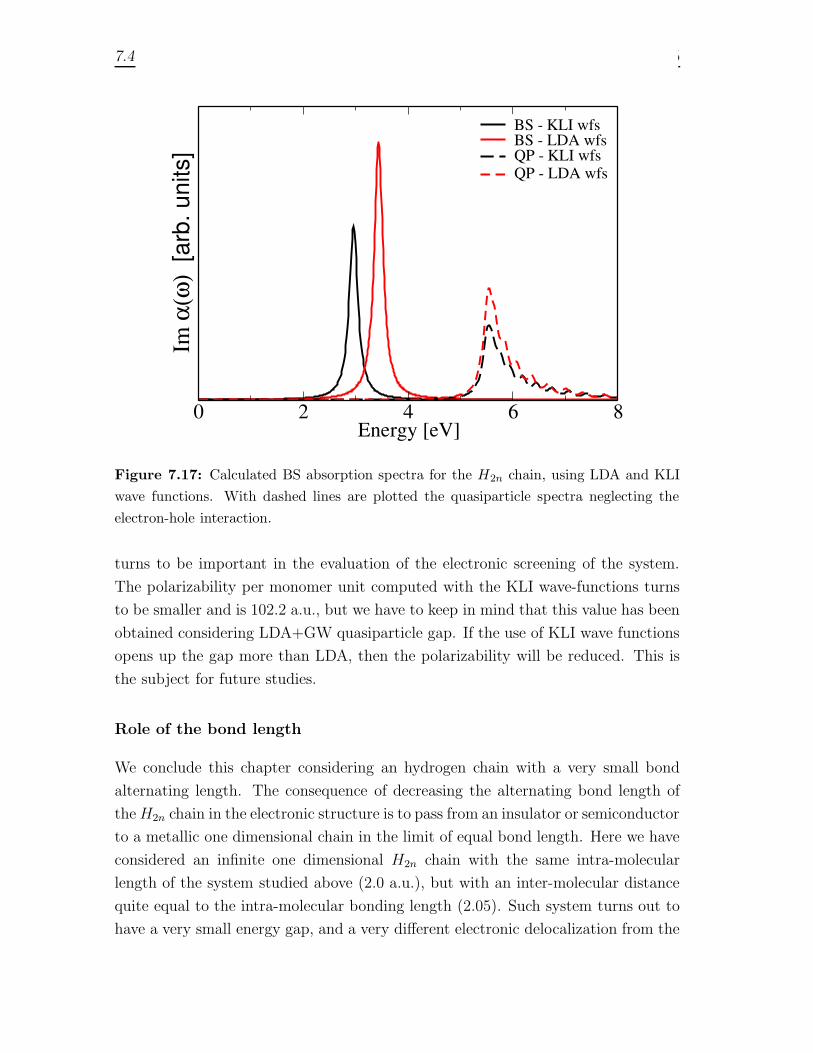
7.4 Infinite chains 155
0 2 4 6 8Energy [eV]
Im α
(ω)
[arb
. uni
ts]
BS - KLI wfsBS - LDA wfsQP - KLI wfs QP - LDA wfs
Figure 7.17: Calculated BS absorption spectra for the H2n chain, using LDA and KLI
wave functions. With dashed lines are plotted the quasiparticle spectra neglecting the
electron-hole interaction.
turns to be important in the evaluation of the electronic screening of the system.
The polarizability per monomer unit computed with the KLI wave-functions turns
to be smaller and is 102.2 a.u., but we have to keep in mind that this value has been
obtained considering LDA+GW quasiparticle gap. If the use of KLI wave functions
opens up the gap more than LDA, then the polarizability will be reduced. This is
the subject for future studies.
Role of the bond length
We conclude this chapter considering an hydrogen chain with a very small bond
alternating length. The consequence of decreasing the alternating bond length of
theH2n chain in the electronic structure is to pass from an insulator or semiconductor
to a metallic one dimensional chain in the limit of equal bond length. Here we have
considered an infinite one dimensional H2n chain with the same intra-molecular
length of the system studied above (2.0 a.u.), but with an inter-molecular distance
quite equal to the intra-molecular bonding length (2.05). Such system turns out to
have a very small energy gap, and a very different electronic delocalization from the
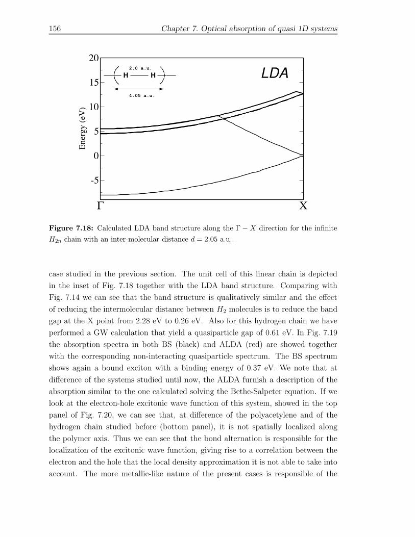
156 Chapter 7. Optical absorption of quasi 1D systems
Γ X
-5
0
5
10
15
20
Ener
gy (e
V)
LDAH H2.0 a.u.
4.05 a.u.
Figure 7.18: Calculated LDA band structure along the Γ − X direction for the infinite
H2n chain with an inter-molecular distance d = 2.05 a.u..
case studied in the previous section. The unit cell of this linear chain is depicted
in the inset of Fig. 7.18 together with the LDA band structure. Comparing with
Fig. 7.14 we can see that the band structure is qualitatively similar and the effect
of reducing the intermolecular distance between H2 molecules is to reduce the band
gap at the X point from 2.28 eV to 0.26 eV. Also for this hydrogen chain we have
performed a GW calculation that yield a quasiparticle gap of 0.61 eV. In Fig. 7.19
the absorption spectra in both BS (black) and ALDA (red) are showed together
with the corresponding non-interacting quasiparticle spectrum. The BS spectrum
shows again a bound exciton with a binding energy of 0.37 eV. We note that at
difference of the systems studied until now, the ALDA furnish a description of the
absorption similar to the one calculated solving the Bethe-Salpeter equation. If we
look at the electron-hole excitonic wave function of this system, showed in the top
panel of Fig. 7.20, we can see that, at difference of the polyacetylene and of the
hydrogen chain studied before (bottom panel), it is not spatially localized along
the polymer axis. Thus we can see that the bond alternation is responsible for the
localization of the excitonic wave function, giving rise to a correlation between the
electron and the hole that the local density approximation it is not able to take into
account. The more metallic-like nature of the present cases is responsible of the
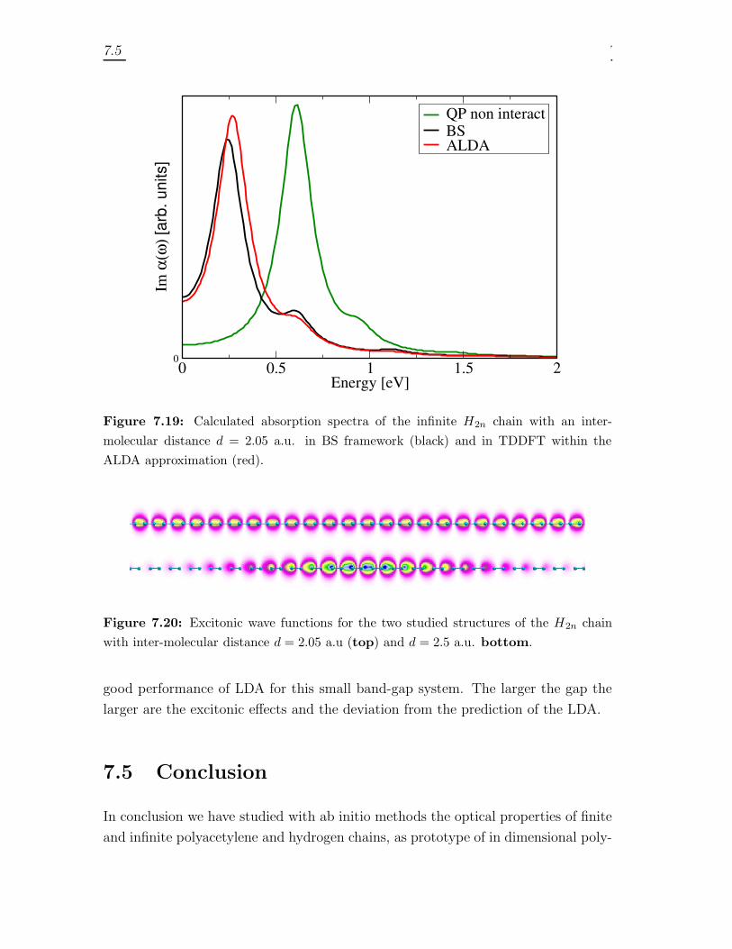
7.5 Conclusion 157
0 0.5 1 1.5 2Energy [eV]
0
Im α
(ω) [
arb.
uni
ts]
QP non interactBSALDA
Figure 7.19: Calculated absorption spectra of the infinite H2n chain with an inter-
molecular distance d = 2.05 a.u. in BS framework (black) and in TDDFT within the
ALDA approximation (red).
Figure 7.20: Excitonic wave functions for the two studied structures of the H2n chain
with inter-molecular distance d = 2.05 a.u (top) and d = 2.5 a.u. bottom.
good performance of LDA for this small band-gap system. The larger the gap the
larger are the excitonic effects and the deviation from the prediction of the LDA.
7.5 Conclusion
In conclusion we have studied with ab initio methods the optical properties of finite
and infinite polyacetylene and hydrogen chains, as prototype of in dimensional poly-

158 Chapter 7. Optical absorption of quasi 1D systems
mers. For these class of systems it is known that the TDDFT when used with the
local and gradient corrected density functionals, does not give an adequate descrip-
tion. We have performed calculations in many body perturbation theory including
electron-hole interactions and in TDDFT using a new non-local and energy depen-
dent kernel. We have showed that this new kernel that until now had been tested
on bulk system and surfaces gives very good results also for finite and quasi one
dimensional systems when compared to the Bethe Salpeter results. Minor discrep-
ancies encountered for small systems can be associated to the effect of the direct
term on the coupling part of the excitonic Hamiltonian (usually neglected for bulk
calculations) that it is not taken into account in the construction of the kernel. The
great overestimation of the ALDA in the calculation of the polarizability for isolated
monomer units is partially corrected when the new kernel is used and we argue that
the the polarizability of finite chains approach the infinite limit when the length of
the chain reach the characteristic length of the size of the exciton of the infinite
chain. Such localization of the electron-hole wave function is due to the bond alter-
nation of the polymer and dictates the saturation of the static polarizability with
polymer length.
8 Photo-electron spectroscopy in
TDDFT framework †
Photo-electron spectroscopy (PES) is a widely used technique to analyze the elec-
tronic structure of complex systems 1 The advent of high intense ultra-short laser
sources have extended the range of applicability of this technique to a vast variety
of non-linear phenomena like high harmonic generation, above threshold ionization
(ATI), bond softening and vibrational population trapping [Brabec 00, Protopapas 97,
Eberly 91]. Furthermore, it has turned femtosecond time-resolved pump-probe PES
as a powerful technique for the characterization of the excite-stated dynamics is
nanostructures and biological systems [Zewail 94, Schattke 03]. n this chapter we
will concentrate on the ATI spectrum [Agostini 79]. It consists in the ionization
of atoms, due by the absorption of a number of photons larger than the needed to
overcome the ionization threshold. Clearly a high intensity laser is needed and in
consequence it is intrinsically a non linear process. The quantity that is measured
in the experiment is the energy of the ejected photoelectrons and the spectrum
typically presents a number of peaks separated by the photon energy. In general,
laser-atom-electron interaction is difficult to treat and approximations are usually
done, as treating the fields classically in the dipolar coupling. Those approxima-
tions are quite good in the strong-field regime that is relevant for those experi-
ments (short-laser pulses with high peak intensities). In this context it is clear
that we need a theory that goes beyond the standard Fermi-Golden rule used to
describe theoretically PES: photon-field matrix elements between the occupied ini-
tial state and the excited outgoing-wave state. This approach is justified only for
low intensity and long laser pulses. For high intensity laser pulses (intensity above
1013Wcm−2) perturbative treatments are no longer suitable because the laser field
† This section is largely an adaptation of the article: D. Varsano, M.A.L Marques, H. Appel,
E.K.U. Gross and A. Rubio: Photo-electron spectroscopy: a TDDFT approach Un-
published. As such, the reported work includes collaboration of the rest of the authors of the
article.1 For recent theoretical and experimental reviews see the following Refs. [Schattke 03, Petek 00,
Almbladh 83, Onida 02] and references therein.
159
160 Chapter 8. Photo-electron spectroscopy in TDDFT framework
becomes comparable with the Coulomb binding field and non-linear effects arise 2.
A fully many-body description of PES is prohibited, except for the cases of few (one
or two) electron systems [Grobe 93, Lein 01, Bandrau 03, Faisal 87] and specific
core level excitations [Schattke 03, Almbladh 83]. Therefore, it will be desirable to
have a PES theory based on Density Functional Theory (DFT) where the complex
many body problem is mapped onto a fictitious single electron system. This is the
purpose of the work presented in this chapter: to circumvent the PES many-body
problem by describing photo-electron emission process within a time-dependent-
density-functional (TDDFT) based geometrical-scheme that address directly the
photo-electron current without resorting to linear response. Other works have been
published addressing single and multiple ionization processes within TDDFT, as for
example Refs. [Maitra 01, Pohl 00, Ullrich 00, V.Veniard 03].
Time-dependent density functional theory (TDDFT), as exposed in the previous
chapter, maps the whole many body problem into the time dependence of the density
from which all physical properties can be obtained. The method is in principle ex-
act, however approximations have to be made for the unknown exchange-correlation
functional as well as for the specific density-functional that provides the physical
quantity we are looking for, in particular even if we know how to formally extract
optical absorption and emission spectra from the time-evolution of the dipole mo-
ment as shown in section (2.2.2), we do not know how to express formally the photo-
electron current in terms only of the time-dependent density. Although it would be
desirable to determine the form of the unknown functional of the density describing
the PES, the purpose of this work is to derive a feasible and working scheme to com-
pute the PES of an interacting electron system in terms of the time-dependent single
electron Kohn-Sham orbitals. For independent electrons the derived formula is ex-
act and for interacting electrons we provide formal justification of the equation for
PES based on the propagation of the many-body density matrix. The idea behind
the present work is to follow the TDDFT Kohn-Sham states under the influence of
the external time-dependent laser field. We have implemented this formalism and
performed the calculations solving the TDDFT Kohn-Sham equations in real time
and real-space. The motivation to work with a grid comes from the flexibility in
describing systems that undergo rearrangements and/or bound-to-continuum tran-
sitions and their adaptation to the present fast time-evolution algorithms. Exchange
2 The electric field that an electron feels in a hydrogen atom, at the distance of one Bohr from
the nucleus is E = e/(4πε0a20 = 5.1× 10⁹V/m. The laser intensity that corresponds to this field
is given by I = ε0cE2/2 = 3.51× 10¹⁶W/cm2.

8.1 One-electron spectroscopy 161
correlation effects will be described using optimized-effective-potentials (TDOEP).
This chapter is organized as follows: in section (8.1) we will describe our approach
to calculate the PES in a single-electron picture. In section (8.2 we will give the
justification of our approach for a many body problem and finally in section (8.3)
we will show the results obtained for a one-dimensional Helium atom model.
8.1 One-electron spectroscopy
Before discussing the main results of the present work, it is important to summarize
how the PES can be exactly calculated for a one-electron system once it is perturbed
by an external laser-pulse. A lot of work has been done in the past to handle this
problem and we refer the reader to references [Brabec 00, Protopapas 97, Faisal 87]
for more details.
The most direct and intuitive way to access the PES is to resort to a wave function
projection scheme in which all bound-state components of the wave function are
projected out; the remaining part gives access to the total electron emission. This
approach relies on the fact that during the laser pulse none of the electrons reach the
detector, all electron current is measured once the laser is turn-off. By monitoring
the time evolution of that projected wave-function we can extract the energy resolved
PES by performing a Fourier transform from time to energy. Another equivalent
approach starts from the the exact many body wave function |ψ〉 after the the laser
field has been turn-off. The PES will be given just by the following projection of
the time-dependent wave-function:
P (E) = |〈Φ(E)|ψ〉|2 = 〈ψ|D(E)|ψ〉 (8.1)
where Φ(E) denotes the wave function of an outgoing (unbound) electron of energy
E of the laser free Hamiltonian, and D(E) is the corresponding projector operator
to this continuum of states. Although no time-propagation has to be performed
once the laser-field is switched-off, to use this formula we encounter two practical
problems: i) we need to know beforehand all the states with positive energy , ii) the
final wave-function extends over a large region of space and therefor large simulation
boxes will be required to describe it properly, complicating the numerical calculation.
These difficulties can nevertheless be overcome for spherical systems using the so-
called window operator approximation to D(E) [Schafer 91]:
D(E) =Γ2n
(H0 − E)2n + Γ2n(8.2)

162 Chapter 8. Photo-electron spectroscopy in TDDFT framework
where Γ and n are parameters controlling the broadening of the spectrum, and H0 is
the ground state Hamiltonian of the system (the resolution of the spectrum is 2Γ).
It was found that n = 2 provides a good description of the spectrum [Schafer 91].
To extend such a procedure for a many electrons system is not at all trivial even if
we can formally define as in Eq. (8.2) a projector operator for a many body system:
D(E) =∑
i
|Φ(E)ΨN−1i 〉〈Φ(E)ΨN−1
i | (8.3)
where |Φ(E)ΨN−1i 〉 is the tensorial product between the ket of the bounded (many-
body) states of the N−1 electron system ΨN−1i and the ionized electron with positive
energy E. Anyway such procedure is very cumbersome and really unpractical to
compute for a general many-electron system, as nanostructures or biomolecules.
Inclusion of exchange-correlation effects for a many-electron interacting-system
can be achieved within TDDFT where we keep the simplicity of working with a set
of time-dependent fictitious single-particle Kohn-Sham orbitals. In spite of having
transferred all the many-body problem into an unknown exchange-correlation func-
tional, the lack of a density-functional that provides the electron emission probability
is, in principle, a major limitation to directly access the PES from the time-evolution
of the density. Therefore, we have to devise a practical scheme that will allow the
extraction of PES from the time-evolution of the Kohn-Sham wave-functions.
Within the standard adiabatic approximation to TDDFT there has been few
attempts to describe PES and multiple ionization processes [Maitra 01, Pohl 00,
Ullrich 00]. All those calculations use the geometrical concept of analyzing box
(depicted in the upper part of Fig. 8.1) to separate the bound and continuum
parts of the many-body wave functions. Then the emission probability is corre-
lated to the change in the number of bound electrons in time (as done for exam-
ple in refs. [Maitra 01, Ullrich 00]). An alternative and very simple scheme was
proposed in ref. [Pohl 00]. The idea is to record the single-electron (Kohn-Sham)
wave-function over time at a point rbc far from the physical system. By Fourier
transforming the time-dependent orbitals into the energy domain: ψi(rbc, E) the
probability of detecting one electron with energy E is given by:
P (E) =∑
i
|ψi(rbc, E)|2 . (8.4)
This method is certainly very easy to implement, nevertheless suffers from some
drawbacks: the weights of the peaks depends on the measuring point rbc, it is
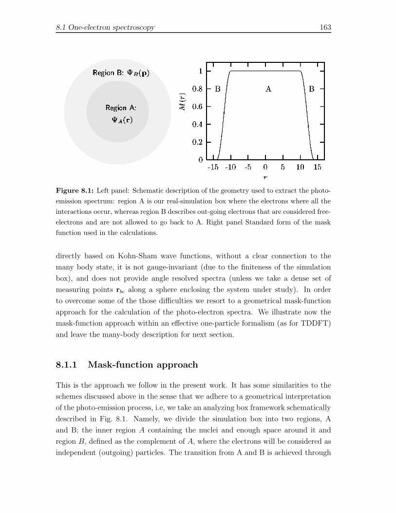
8.1 One-electron spectroscopy 163
Figure 8.1: Left panel: Schematic description of the geometry used to extract the photo-
emission spectrum: region A is our real-simulation box where the electrons where all the
interactions occur, whereas region B describes out-going electrons that are considered free-
electrons and are not allowed to go back to A. Right panel Standard form of the mask
function used in the calculations.
directly based on Kohn-Sham wave functions, without a clear connection to the
many body state, it is not gauge-invariant (due to the finiteness of the simulation
box), and does not provide angle resolved spectra (unless we take a dense set of
measuring points rbc along a sphere enclosing the system under study). In order
to overcome some of the those difficulties we resort to a geometrical mask-function
approach for the calculation of the photo-electron spectra. We illustrate now the
mask-function approach within an effective one-particle formalism (as for TDDFT)
and leave the many-body description for next section.
8.1.1 Mask-function approach
This is the approach we follow in the present work. It has some similarities to the
schemes discussed above in the sense that we adhere to a geometrical interpretation
of the photo-emission process, i.e, we take an analyzing box framework schematically
described in Fig. 8.1. Namely, we divide the simulation box into two regions, A
and B; the inner region A containing the nuclei and enough space around it and
region B, defined as the complement of A, where the electrons will be considered as
independent (outgoing) particles. The transition from A and B is achieved through

164 Chapter 8. Photo-electron spectroscopy in TDDFT framework
a smooth mask function M(r) which is defined to be 1 deep in the interior of A and 0
outside (see Fig. 8.1(right panel)). The advantage of using such approach is that we
can store the wave-function in a spatial mesh inside A, while in B the free-electrons
can be trivially treated in momentum space. The time evolution is performed in
the velocity gauge in order to avoid numerical instabilities at the boundary of the
analyzing box. During time evolution part of the density contained in A will go to
region B, and from that moment on it will be assumed to be ionized. This is taken
into account at each iteration using a smooth mask function M(r) that acts directly
to the time-dependent wave-function. The evolution scheme is the following:
ψAi (r, t+ ∆t) = M(r)e−iH∆tψAi (r, t)
ψBi (p, t+ ∆t) = e−i(p−A(t))2
2∆tψBi (p, t) + ψAi (p, t + ∆t) (8.5)
where H is the single-particle Hamiltonian, A(t) is the vector potential associated
to the electric field of the laser pulse,and ψAi (p, t + ∆t) is the Fourier transform of
the part of the wave function ψAi that have left the region A in the time step ∆t i.e:
ψAi (p, t + ∆t) =
∫
dr(1 −M(r))e−iH∆tψAi (r, t)eip·r (8.6)
The evolution is performed until no appreciable density leaves region A. In this
scheme there is no constrain about when the electron is emitted, either during or
after the laser pulse has been applied, however the simulation box A has to be large
enough in order to minimize the error stemming from neglecting the possibility that
electrons in region B come back into region A. This size would clearly depend on
the laser parameters: intensity, frequency and pulse shape.
As the electrons in region B of the simulation box are considered free it is tempt-
ing to identify these as photo-electrons, and then write momentum-resolved photo-
electron spectra as:
P (p) =∑
i
|ψBi (p, t→ ∞)|2 (8.7)
the total kinetic-energy PES is obtained integrating over angles Eq. (8.7):
P (Ep = p2/2) =
∫
dΩp
∑
i
|ψBi (p, t→ ∞)|2 , (8.8)
similarly, the angle-resolved spectra comes straightforwardly through a partial inte-
gration with respect to the absolute momentum transfer p:
P (θp, φp) =
∫
dp∑
i
|ψBi (p, t→ ∞)|2 , (8.9)

8.2 Many-body photo-electron spectroscopy 165
where the momentum angular coordinates θp, φp are held fixed in a given reference
frame. For non-interacting electrons, the calculation of PES using Eqs.(8.7-8.9) is
formally correct as the only real approximation is neglecting the recoiling of electrons
that reach region B while the laser is on, however this can be easily control by
changing the size of A. However, in this case also the much simpler approach or
Ref. [Pohl 00] described in Eq. (8.4) will provide an exact description of the total
photo-electron current. On the other hand, for an interacting many-body system
it would be desirable to provide some formal justification of Eq. (8.7) besides the
heuristic approach described here. This is done in the following section where we
establish a link between the photo-electron current and the time evolution of the
interacting many-body density-matrix.
8.2 Many-body photo-electron spectroscopy
As for one-electron system, the knowledge of the time evolution of the many-body
wave function contain the relevant information to compute the PES. The most direct
approach would be to project out all bound-state components and the remaining is
the desired integrated photo-electron spectra. Of course, this scheme is not practical
for many-electron systems as we need not only the full-time-dependent wave function
but also the complete knowledge of the whole bound-state spectra (see Eqs.8.3).
Still, it is illustrative to show how we could get around the problem of the bound
states by using once more the geometrical approach of Fig. 8.1 discussed in the
previous section. Let us illustrate the scheme for the case of two-electron system
perturbed by a short-laser-pulse. The mask function should be applied only to one
of the two spatial coordinates for the wave-function, as integrating over the other
coordinate will provide the emission probability, or more precisely, the probability of
having one electron in region B. In practice, we evolve in time the wave-function in
region A with the full two-electron Hamiltonian H, mask the second coordinate and
Fourier transform to momentum space the part of the wave-function (ψAi ) leaving
region A:
ψA(r1, r2, t+ ∆t) = (1 −M(r2))e−iH∆tψA(r1, r2, t)
ψA(r1,p, t+ ∆t) =
∫
dr2ψA(r1, r2, t+ ∆t)eip·r2
ψB(r1,p, t+ ∆t) = e(−iH1+ 12(p2−A(t))2)∆tψB(r1,p, t)
+ψA(r1,p, t+ ∆t) (8.10)

166 Chapter 8. Photo-electron spectroscopy in TDDFT framework
where now the Hamiltonian that controls the time-evolution does not have the
electron-electron repulsion term and the propagation of coordinate 2 is assumed
to be the one corresponding to a free-particle whereas coordinate 1 evolves with
the remaining H1 part of the full-Hamiltonian H = H1 + H2 + V (1, 2). Now the
photo-electron spectra reads:
P (p) = limt→∞
∫
dr1|ψB(r1,p, t)|2 . (8.11)
Therefore we only need to accumulate in time the wave-function in region B. Of
course Eq. (8.11) reduces to Eq. (8.7) in the case of independent electrons. Still this
approach for general interacting electron systems is computationally unpractical and
one would like to use Eq. (8.7) for PES calculations. In the next two sections we
will try to provide a formal justification for this approach by looking at the time-
evolution of the Wigner transform of the one-body density matrix and by performing
a simple population analysis, i.e. looking how many electrons leave the arbitrary
simulation box.
8.2.1 Density-matrix approach
The one-body density matrix of the system of N particles is defined as:
n(r, r′) =
∫
d(r2...rN)Ψ(r, r2, ..., rN)Ψ?(r′, r2, ..., rN) , (8.12)
where Ψ denotes the full many-body wave-function. This expression is simplified
if one works with independent particles; in this case Ψ is a Slater determinant and
Eq. (8.12) reduces to: n(r, r′) =∑occ
i ψi(r)ψ?i (r
′), with ψ the one-body orbitals
that in the case of DFT, they correspond to the Kohn-Sham eigenfunctions. It is
important to note that the Kohn-Sham density matrix is not equal to the full many-
body density matrix even if their diagonals (i.e. the density) are equal. This can
be seen from the fact that the Kohn-Sham is idempotent whereas the exact one is
not. The probability of finding a N-electron system in one of its possible (positive)
charge states, related to electron emission, can be formally written [Ullrich 00], but
simplifications are due to have a formulation in terms of KS single particle orbitals.
In order to make connection with a classical description of photo-electron emission,
it is convenient to extend the classical concept of phase-space distribution to the
quantum regime. A common approximation for a quantum phase-space distribution
function comes from the the Wigner transform of the density matrix with respect

8.2 Many-body photo-electron spectroscopy 167
the center of mass coordinate R = (r+r′)/2. This Wigner transformation is defined
as [Baym 62]
w(R,p) =
∫
dseip·sn(R + s/2,R− s/2), (8.13)
where s = r − r′ is the relative position. This function it is normalized and its
integral over the whole space (momentum) give the probability density to finding
an electron with momentum p (position R):
∫
d3p
(2π)3w(R,p) =
∫
d3p
(2π)3
∫
d3seip·sn(R + s/2,R− s/2)
=n(R,R) = n(R) (8.14)
∫
d3Rw(R,p) =
∫
d3R
∫
d3seip·sn(R + s/2,R − s/2)
=
∫
d3(r2...rN)|Ψ(p, r2...rN)|2 = n(p). (8.15)
Note that uncertainty principle prevents the knowledge of r and p simultaneously,
therefore w(R,p) cannot be a proper joint distribution function. Assuming now that
the Wigner function in Eq. (8.13) is a good approximation for the joint-distribution
function, we can use the geometrical procedure discussed in previous section and
monitor in region B of Fig. 8.1 the time-evolution of the joint-distribution function
for the system of interest. In this case we can resort to the classical definition of
photo-electron spectra (PES) based on the knowledge of the phase-space distribution
function:
P (E = p2/2) =
∫
B
dRw(R,p) (8.16)
In this Eq. (8.16) the function w(R,p) should be evaluated a long time after the
laser has been turn off in order to have all the ionized density contained in region
B.
At this point we should make contact with an effective single-particle theory as
TDDFT and derive the equivalent equation of Eq. (8.16) for Kohn-Sham orbitals.
It is clear from our previous discussion that the stationary one-body Kohn-Sham
density matrix is given by
nKS(r, r′) =
occ.∑
i=1
ψi(r)ψ?i (r
′) (8.17)
168 Chapter 8. Photo-electron spectroscopy in TDDFT framework
The density matrix (8.17) can be written in the following way:
nKS(r, r′) =
∑
i
[
ψAi (r)ψA?i (r′) + ψAi (r)ψB?i (r′)
+ψBi (r)ψA?i (r′) + ψBi (r)ψB?i (r′)
]
(8.18)
We can see that first term, containing the product of the wave function in region A,
does not contribute to the integral of Eq. (8.16). We expect that the contribution
of the next two terms that correspond to overlaps of a localized wave function with
an unlocalized is negligible, so Eq. (8.16) reads:
P (E) '∫
B
dR
∫
dseip·s∑
i
ψBi (R + s/2)ψB?i (R− s/2) (8.19)
As the probability of finding an ionized electron in the region A is small we can
extend the integration over B to the whole space and after some algebra we obtain:
P (E) '∑
i
|ψBi (p)|2 . (8.20)
We have found the same Eq. (8.7) as the wave-functions appearing in Eq. (8.20)
correspond to the evaluation of the Wigner function long after the pulse has been
switch off (t→ ∞).
8.2.2 Population analysis
We have already derived Eq. (8.20) following two different paths. Here we add
another one by looking at the time evolution of the number of electron leaving a
region delimited by a surface S (where the molecule is situated):
NS(t1) = 1 −∫
ΩS
drn(r, t1) = −t1∫
t0
dt
∫
ΩS
drn(r, t), (8.21)
where with ΩS we have indicated the volume contained in the surface S, and t0 is
a time before the laser is switched on and the total charge density of the system
is still inside the surface S. Using the continuity equation the number of electrons
leaving S is given by:
NS(t1) = −t1∫
t0
dt
∫
ΩS
dr∇ · j(r, t) (8.22)
8.2 Many-body photo-electron spectroscopy 169
Using the relation that connect the current j to the Wigner function defined in
Eq. (8.13):
j(r, t) =
∫
dp
(2π)3pw(r,p, t) (8.23)
we can express the NS as
NS(r1) =
∫
dp
(2π)3
t1∫
t0
dt
∫
ΩS
dr∇ · pw(r,p, t)
≡∫
dp
(2π)3P (p) . (8.24)
We can analyse the quantity inside the square bracket in Eq. (8.24) as the desired
photo-electron spectrum. This can be make more clear by using Gauss theorem to
convert the volume integral in Eq. (8.24) into a surface integral; thus the photo-
electron spectrum reads
P (p) =
t1∫
t0
dt
∫
S
dApw(r,p, t) . (8.25)
So, we are measuring the current passing through a surface S far away from the sys-
tem, that is a very intuitive image of an ionization process. Until now all derivation
has been general, now in order to get a manageable expression we approximate the
Wigner function by its Kohn-Sham counterpart (as in the previous section). After
inserting the Fourier transforms of the Kohn-Sham wave functions we get:
w(r,p, t) =∑
i
∫
dk
(2π)3e−2i(k−p)·rψBi (k, t)ψB?i (2p − k, t). (8.26)
Using the fact that after the laser is switched-off the electrons outside S (region B
in Fig. 8.1) propagate in time as free particles:
ψBi (k, t) = e−ik2
2(t−t0)ψB
i (k,t0) (8.27)
gathering Eqs.(8.24),(8.26),(8.27) we obtain:
P (p) =∑
i
t1∫
t0
dt
∫
ΩS
dr
∫
dk
(2π)3[−2i(k−p)] · pe−i
(
k2
2− (2p−k)2
2
)
t×
× e−2i(k−p)·rψBi (k)ψB?i (2p − k) (8.28)
170 Chapter 8. Photo-electron spectroscopy in TDDFT framework
where we have put t0 = 0 for sake of simplicity. Now we can perform analytically
the integration over time in the limit t1 → ∞ and then take the limit of the radius
of the sphere RS → ∞. 3 Taking into account the result:
∞∫
0
dte−iεt =i
ε(8.29)
we obtain:
P (p) =∑
i
∫
ΩS
dr
∫
dk
(2π)32(k − p)] · p e−2i(k−p)·r
k2
2− (2p−k)2
2
ψBi (k)ψB?i (2p − k) (8.30)
If we now perform the limRS → ∞, and integrate r over all space, we get:
P (p) =∑
i
∫
dk
(2π)32(k − p)] · p δ(k − p)
k2
2− (2p−k)2
2
ψBi (k)ψB?i (2p − k)
=∑
i
|ψBi (p)|2. (8.31)
and Eq. (8.7) is once more obtained.
3 we note here that if we first take the limit RS → ∞ , and perform the space integral, we will
get zero as one would expect.
8.3 Results 171
8.3 Results
To illustrate how the many-body based procedures work we look a simple one-
dimension two-electrons atom model. It is described by a nucleus of positive charge
fixed at the origin at z = 0 and two electron whose spatial coordinates are indicated
by z1 and z2. Its bare Hamiltonian is:
H0 =1
2p2
1 +1
2p2
2 + V (z1) + V (z2) + V (z1 − z2) (8.32)
Both the attractive electron-ion and the repulsive electron-electron interaction is
modeled by the so-called soft Coulomb potential[Grobe 93].
V (z) = − 1√z2 + 1
(8.33)
The potential (8.33) is a realistic model for ionization studies: it has the correct
coulombic asymptotic behavior and is a way to allowing in 1D for the possibility
that the electrons pass by the nucleus and by each other without probing a Coulomb
singularity. The total potential V (z1, z2) (electron-ions and electron-electron inter-
action) is plotted in Fig. 8.2. We see that the potential is symmetric with respect the
z1 = z2 and z1 = −z2 diagonals and the ”hill” along z1 = z2 indicates that it is not
energetically favorable to find both electrons on the same side of the nucleus. Now
we apply a laser pulse, the time-dependent velocity-gauge Schrodinger equation, in
atomic units, for the two electron wave function Ψ(z1, z2, t) is:
i∂Ψ
∂t(z1, z2, t) =
[
2∑
i=1
(
(
pi − A(t))2
2− 2√
z2i + 1
)
++1
√
(z1 − z2)2 + 1
]
Ψ(z1, z2, t)
(8.34)
where zi are the electrons coordinates, pi are the canonical electron momenta and
A(t) = −∫ t
0ε(t′)dt′ is the vector potential associated to the electric field of the
laser pulse ε(t) = ε0f(t, Tpulse)sin(ωt) with amplitude ε0 and frequency ω. With
f(t, Tpulse) we have indicated an envelope function.
For the Kohn-Sham solution of the problem we use an exact exchange functional
vx(z, t), namely a time-dependent optimized-effective-potential Eq. (1.26) that for
two-electrons is half of the Hartree potential:
vH(z, t) =
∫
n(z′, t)√
(z − z′)2 + 1dz′ (8.35)
vx(z, t) = −1
2vH(z, t) (8.36)

172 Chapter 8. Photo-electron spectroscopy in TDDFT framework
-1.5
-1
-0.5
0
0.5
1
-40-20
0 20
40
-40-20
0 20
40
0
tvuxwzy|z~it wzyz~i
t u t A
Figure 8.2: The total potential V (z1, z2) as a function of the two one-dimensional electron
coordinates z1 and z2.
i.e. the Kohn-Sham Hamiltonian is
HKS =(p− A(t))2
2− 2√
z2 + 1+ vH(z, t) + vx(z, t) . (8.37)
For this simple case we can perform the time evolution of this one-dimensional soft-
core He atom exact Eq(8.34), and within the TDOEP approximation Eq(8.37). The
time-evolution of the wave function has been performed following the split-operator
method [Feit 82]: the unitary evolution operator U(t − t0) = exp[−iH(t − t0)], for
a small increment time-step can be decomposed in three steps as:
U(∆t) = e−i(T+V )∆t = e−iT∆t2 e−iV∆te−iT
∆t2 +O(∆3) (8.38)
The action of the kinetic energy operator is easily performed in Fourier space 4.
The ground state wave function Φg(z1, z2) is computed evolving always according
to Eq. (8.38) the Schrodinger equation (8.34) replacing the time-step ∆t by an
imaginary time-step −i∆τ . In this way any arbitrary initial seed function relaxes
to the ground state wave function after a sufficient amount of imaginary time.
4 If we write the action of the electromagnetic field in velocity gauge as in Eqs (8.34 and 8.37),
the term exp[−i (p−A(t))2
2 ] is treated in Fourier space.

8.3 Results 173
0.1 0.01 0.001
0.0001 1e-05 1e-06 1e-07 1e-08 1e-09 1e-10
-10 -5 0 5 10
-10
-5
0
5
10
0.1 0.01 0.001
0.0001 1e-05 1e-06 1e-07 1e-08 1e-09 1e-10
-10 -5 0 5 10
-10
-5
0
5
10
0.1 0.01
0.001 0.0001 1e-05 1e-06 1e-07 1e-08 1e-09 1e-10
-100 -50 0 50 100
-100
-50
0
50
100
0.1 0.01
0.001 0.0001 1e-05 1e-06 1e-07 1e-08 1e-09 1e-10
-100 -50 0 50 100
-100
-50
0
50
100
0.1 0.01 0.001 0.0001 1e-05 1e-06 1e-07 1e-08 1e-09 1e-10
-100 -50 0 50 100
-100
-50
0
50
100
0.1 0.01 0.001 0.0001 1e-05 1e-06 1e-07 1e-08 1e-09 1e-10
-100 -50 0 50 100
-100
-50
0
50
100
Figure 8.3: Snapshots of the probability density for He soft core. The two axis represents
the coordinates of the two electrons. Exact (left panel) and TDOEP (right panel). Upper
panel: ground state. Middle panel, the laser pulse in turned on (after 5 optical cycle).
Bottom panel: End of the pulse (40 optical cycles).
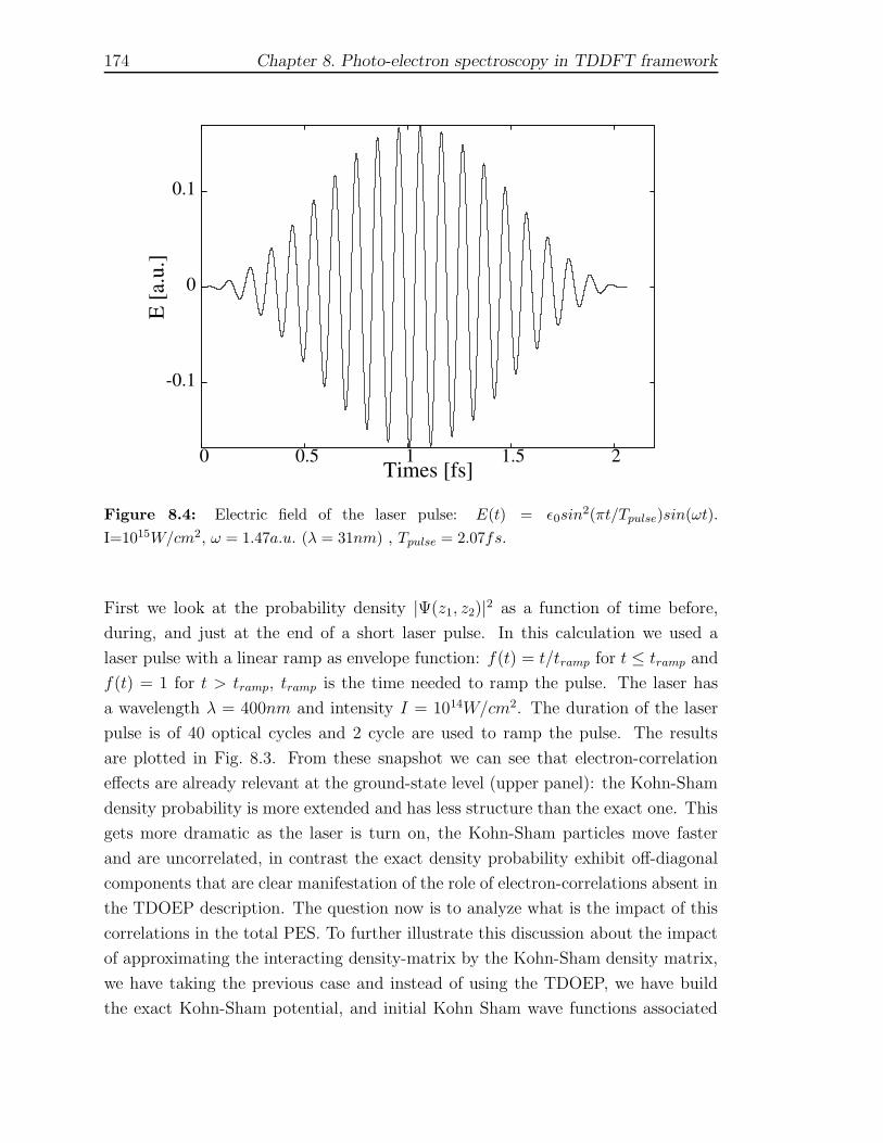
174 Chapter 8. Photo-electron spectroscopy in TDDFT framework
-0.1
0
0.1
0 0.5 1 1.5 2
E [a
.u.]
Times [fs]
Figure 8.4: Electric field of the laser pulse: E(t) = ε0sin2(πt/Tpulse)sin(ωt).
I=1015W/cm2, ω = 1.47a.u. (λ = 31nm) , Tpulse = 2.07fs.
First we look at the probability density |Ψ(z1, z2)|2 as a function of time before,
during, and just at the end of a short laser pulse. In this calculation we used a
laser pulse with a linear ramp as envelope function: f(t) = t/tramp for t ≤ tramp and
f(t) = 1 for t > tramp, tramp is the time needed to ramp the pulse. The laser has
a wavelength λ = 400nm and intensity I = 1014W/cm2. The duration of the laser
pulse is of 40 optical cycles and 2 cycle are used to ramp the pulse. The results
are plotted in Fig. 8.3. From these snapshot we can see that electron-correlation
effects are already relevant at the ground-state level (upper panel): the Kohn-Sham
density probability is more extended and has less structure than the exact one. This
gets more dramatic as the laser is turn on, the Kohn-Sham particles move faster
and are uncorrelated, in contrast the exact density probability exhibit off-diagonal
components that are clear manifestation of the role of electron-correlations absent in
the TDOEP description. The question now is to analyze what is the impact of this
correlations in the total PES. To further illustrate this discussion about the impact
of approximating the interacting density-matrix by the Kohn-Sham density matrix,
we have taking the previous case and instead of using the TDOEP, we have build
the exact Kohn-Sham potential, and initial Kohn Sham wave functions associated

8.3 Results 175
Figure 8.5: Difference in absolute value between the one-body density matrix of the
many body system and the Kohn-Sham system Eq. (8.17) at initial time (on the left) and
after the interaction of the system (on the right) with a laser pulse of 20 cycles at intensity
I = 1015W/cm2 and ω = 1.47a.u. (λ = 31nm). in a square of 16 a.u. around the origin
Fig. 8.4.
to the initial many-body density: ψks =√
ngs/2. In this case we have used a laser
pulse of 20 cycles with a wavelength λ = 31nm and intensity I = 1015W/cm2.
The envelope function is of the form: f(t) = sin2(πt/Tpulse). The laser pulse is
showed in Fig. 8.4. Then we propagate the Kohn-Sham system with a TDOEP only
exchange potential. In Fig. 8.5 we show the difference in absolute value between
the one-body density matrix of the many body system and the Kohn-Sham system
(Eq. (8.17)) before and after the interaction with the laser field. We can see that at
initial time (left part of the figure) the diagonal (i.e. the density) turn out to be the
same by construction of the Kohn-Sham system, while after the laser interaction
differs due to the lack of a correlation term in the Kohn-Sham Hamiltonian. If
one does the same analysis done with the density-matrix in section 8.2.1 but now
for a two-electron process, namely two-electron spectroscopy, we would end up in
P (p1,p2) =∑
i |ψBi (p1)|2∑
j |ψBj (p2)|2−∑
ij ψBi (p1)ψ
B∗i (p2)ψ
Bj (p2)ψ
B∗j (p1) for the
case of only two electrons it reduces to P (p1,p2) = |ψB(p1)|2|ψB(p2)|2 which is just
the product of the probability of emitting one particle. Therefore no correlation
in the two-electron process is accounted for. This deficiency should be traced back
to the fact that we approximated the interacting density matrix by its Kohn-Sham
form.
Now we can address how relevant the differences are when the PES is calculated
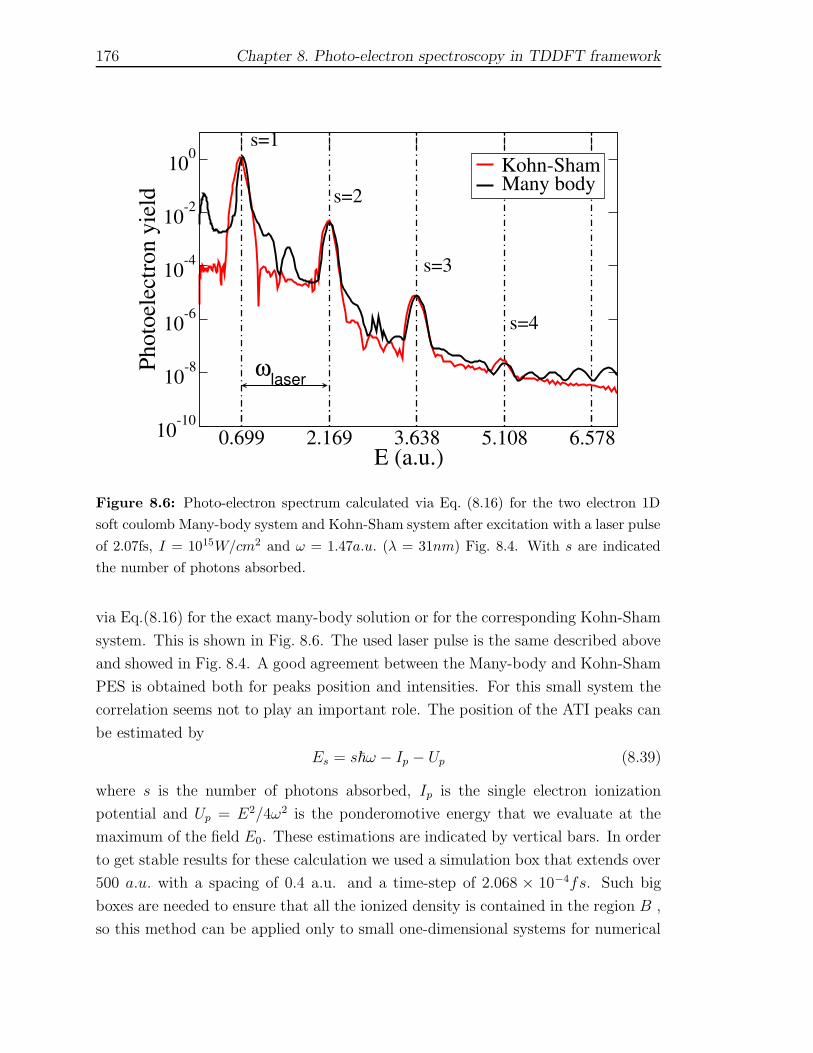
176 Chapter 8. Photo-electron spectroscopy in TDDFT framework
0.699 2.169 3.638 5.108 6.578E (a.u.)
10-10
10-8
10-6
10-4
10-2
100Ph
otoe
lect
ron
yiel
dKohn-ShamMany body
ωlaser
s=1
s=2
s=3
s=4
Figure 8.6: Photo-electron spectrum calculated via Eq. (8.16) for the two electron 1D
soft coulomb Many-body system and Kohn-Sham system after excitation with a laser pulse
of 2.07fs, I = 1015W/cm2 and ω = 1.47a.u. (λ = 31nm) Fig. 8.4. With s are indicated
the number of photons absorbed.
via Eq.(8.16) for the exact many-body solution or for the corresponding Kohn-Sham
system. This is shown in Fig. 8.6. The used laser pulse is the same described above
and showed in Fig. 8.4. A good agreement between the Many-body and Kohn-Sham
PES is obtained both for peaks position and intensities. For this small system the
correlation seems not to play an important role. The position of the ATI peaks can
be estimated by
Es = s~ω − Ip − Up (8.39)
where s is the number of photons absorbed, Ip is the single electron ionization
potential and Up = E2/4ω2 is the ponderomotive energy that we evaluate at the
maximum of the field E0. These estimations are indicated by vertical bars. In order
to get stable results for these calculation we used a simulation box that extends over
500 a.u. with a spacing of 0.4 a.u. and a time-step of 2.068 × 10⁻⁴fs. Such big
boxes are needed to ensure that all the ionized density is contained in the region B ,
so this method can be applied only to small one-dimensional systems for numerical
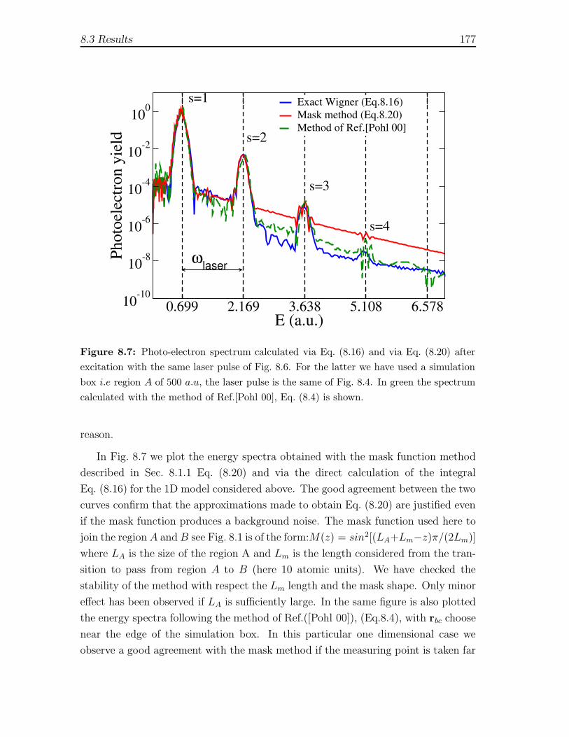
8.3 Results 177
0.699 2.169 3.638 5.108 6.578E (a.u.)
10-10
10-8
10-6
10-4
10-2
100Ph
otoe
lect
ron
yiel
dExact Wigner (Eq.8.16)Mask method (Eq.8.20)Method of Ref.[Pohl 00]
ωlaser
s=1
s=2
s=3
s=4
Figure 8.7: Photo-electron spectrum calculated via Eq. (8.16) and via Eq. (8.20) after
excitation with the same laser pulse of Fig. 8.6. For the latter we have used a simulation
box i.e region A of 500 a.u, the laser pulse is the same of Fig. 8.4. In green the spectrum
calculated with the method of Ref.[Pohl 00], Eq. (8.4) is shown.
reason.
In Fig. 8.7 we plot the energy spectra obtained with the mask function method
described in Sec. 8.1.1 Eq. (8.20) and via the direct calculation of the integral
Eq. (8.16) for the 1D model considered above. The good agreement between the two
curves confirm that the approximations made to obtain Eq. (8.20) are justified even
if the mask function produces a background noise. The mask function used here to
join the region A andB see Fig. 8.1 is of the form:M(z) = sin2[(LA+Lm−z)π/(2Lm)]
where LA is the size of the region A and Lm is the length considered from the tran-
sition to pass from region A to B (here 10 atomic units). We have checked the
stability of the method with respect the Lm length and the mask shape. Only minor
effect has been observed if LA is sufficiently large. In the same figure is also plotted
the energy spectra following the method of Ref.([Pohl 00]), (Eq.8.4), with rbc choose
near the edge of the simulation box. In this particular one dimensional case we
observe a good agreement with the mask method if the measuring point is taken far
178 Chapter 8. Photo-electron spectroscopy in TDDFT framework
off enough the interaction zone.
In conclusion we have presented a non-perturbative approach for the calcula-
tion of the photo-electron spectra that allows to extract integrated above-threshold-
ionization spectra of molecular structures. Within the geometrical concept of the
mask-operator convergent ATI spectra is obtained. Femtosecond time resolved
pump-probe experiments can be modeled withing the present scheme with a very
low computational cost compared with full many-body-based schemes as we will
show in the next chapter. Of course, the lack of good exchange-correlation func-
tionals for strong-non-linear phenomena is a major drawback. This is clearly seen
when trying to describe the non-sequential double ionization yield of He and Ne,
where the experimental results are several orders of magnitude larger than TDDFT
calculations using standard functionals [Petersilka 99, Lappas 98, Bauer 01].
9 Two photon-photoemission
spectra of Cu metal surfaces†
9.1 Introduction
In this chapter we apply the methodology described in the previous chapter for
the calculation of photo-electron-spectroscopy to study Two-Photon Photo-emission
(TPPE) [Giesen 85, Haight 95, Fauster 95] spectra and Time-Resolved Two-Photon
Photo-emission (TR-TPPE) [Schoenlein 88, Schoenlein 90]. In TPPE, intense laser
radiation is used to populate an unoccupied state with the first photon (pump) and
subsequently such electron in the intermediate state is ejected by the second pho-
ton (probe). In TR-TPPE, the probe pulse which ionize the intermediated state
is delayed with respect the pump pulse which populates it, thus providing a direct
measurement of the intermediate state lifetime. Here we want to study the TPPE
and TR-TPPE for two metal surfaces: Cu(100) and Cu(111). The presence of a
metal surface creates electron states that do not exist in the bulk metal. These
states can be classified into two groups, according to their charge density local-
ization with respect the surface atomic layer: crystal-induced and image-potential
induced surface states. The former are localized mainly at the surface atomic layer
[Tamm 32, Shockley 39], while the latter lie mainly in the vacuum region of a metal
surfaces with a band gap near the vacuum level. The symmetry breaking on the
surface is responsible for the so-called crystal-induced surface states, whereas image
states are caused by the long-range tail of the image potential induced at the sur-
face. An electron situated at a distance z from the metal surface experiments an
attractive force, F (z) = −e2/(2z)2, equivalent to that produced by its image charge
situated at distance z inside the metal. For large z, the potential generated by this
surface induced charge approaches the classical image potential, V (z) = −e2/4z.
† This section is largely an adaptation of the article: D. Varsano, M.A.L Marques and A. Rubio:
Time and energy-resolved two photon-photoemission of the Cu(100) and Cu(111)
metal surfaces. Computational Material Science 30, 110 (2004). As such, the reported work
includes collaboration of the rest of the authors of the article.
179

180 Chapter 9. Two photon-photoemission spectra of Cu metal surfaces
-20 0 20 40 60 80 100z (atomic units)
-4
-2
2En
ergy
(eV
)
Elower
EF
Energy gap
p=1p=2 p=3
Image potentialhωa
hωbEvac
unoccupied states
surface state (resonance)
0.080.180.57
3.73
---
-
Figure 9.1: Schematic picture of a TPPE experiment for a typical metallic surface with a
surface band gap close to the Fermi level. The energy ~ωa (red) corresponds to the pump
photon and ~ωb (green) to the probe photon in TPPE. On the right side we show the tail
of the image potential, the densities of the surface state and first three image potential
states of Cu(100) (blue) calculated with the model potential of Ref.[Chulkov 99b], and
their corresponding binding energies. By EF , Elower and Evac we denote respectively the
Fermi energy, the lower edge of the energy gap and the vacuum energy.
This expression corresponds to assuming an infinite repulsive barrier at the surface.
In the more general case we have
V (z) = − e2
4(z − zim)
ε− 1
ε+ 1(9.1)
where zim is the position of the image plane (that depends on the electronic and
structural properties of the surface), and ε is the static dielectric constant of the
surface. When the metal has a surface band gap near the vacuum level, the electrons
below the vacuum level are trapped between the well of the image potential and the
surface barrier. These quantized states correspond to image potential states, and
are spatially localized in the region in front of the surface (see Fig. 9.1). Metal
image states typically have a large spatial extension, but barely penetrate the bulk
metal. They form a Rydberg-like series with energies, Ep, approximately given
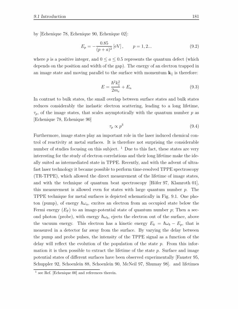
9.1 Introduction 181
by [Echenique 78, Echenique 90, Echenique 02]:
Ep = − 0.85
(p + a)2[eV] , p = 1, 2... (9.2)
where p is a positive integer, and 0 ≤ a ≤ 0.5 represents the quantum defect (which
depends on the position and width of the gap). The energy of an electron trapped in
an image state and moving parallel to the surface with momentum k‖ is therefore:
E =~
2k2‖
2me
+ En (9.3)
In contrast to bulk states, the small overlap between surface states and bulk states
reduces considerably the inelastic electron scattering, leading to a long lifetime,
τp, of the image states, that scales asymptotically with the quantum number p as
[Echenique 78, Echenique 90]
τp ∝ p3 (9.4)
Furthermore, image states play an important role in the laser induced chemical con-
trol of reactivity at metal surfaces. It is therefore not surprising the considerable
number of studies focusing on this subject. 1 Due to this fact, these states are very
interesting for the study of electron correlations and their long lifetime make the ide-
ally suited as intermediated state in TPPE. Recently, and with the advent of ultra-
fast laser technology it became possible to perform time-resolved TPPE spectroscopy
(TR-TPPE), which allowed the direct measurement of the lifetime of image states,
and with the technique of quantum beat spectroscopy [Hofer 97, Klamroth 01],
this measurement is allowed even for states with large quantum number p. The
TPPE technique for metal surfaces is depicted schematically in Fig. 9.1. One pho-
ton (pump), of energy ~ωa, excites an electron from an occupied state below the
Fermi energy (EF) to an image-potential state of quantum number p; Then a sec-
ond photon (probe), with energy ~ωb, ejects the electron out of the surface, above
the vacuum energy. This electron has a kinetic energy Ek = ~ωb − Ep, that is
measured in a detector far away from the surface. By varying the delay between
the pump and probe pulses, the intensity of the TPPE signal as a function of the
delay will reflect the evolution of the population of the state p. From this infor-
mation it is then possible to extract the lifetime of the state p. Surface and image
potential states of different surfaces have been observed experimentally [Fauster 95,
Schuppler 92, Schoenlein 88, Schoenlein 90, McNeil 97, Shumay 98]. and lifetimes
1 see Ref. [Echenique 00] and references therein.

182 Chapter 9. Two photon-photoemission spectra of Cu metal surfaces
of image states for different metal surfaces have been calculated in the framework of
the self-energy formalism in the GW approximation [de Andres 87, de Andres 89,
Osma 99b, Sarria 99, Chulkov 98, Chulkov 97, Echenique 00]. The results obtained
happen to be in rather good agreement with experiments. For example, the calcu-
lated [Echenique 00] lifetime of the first three image potential states of the Cu(100)
surface are τ theor1 = 30 fs, τ theor
2 = 132 fs, and τ theor3 = 367 fs, while the experimental
values [Hofer 97] are τ exp1 = 40±6 fs, τ exp2 = 110±10 fs, and τ exp3 = 300±15 fs, while
for the first image state of Cu(111) surface the theoretical lifetime is τ theor1 = 17.5 fs
and the experimental [McNeil 97] is τ exp1 = 15 ± 5 fs.
In the following sections we will describe the calculations made on energy-
resolved TPPE spectra of Cu(100) and Cu(111) surfaces. The theoretical approach
is based on the propagation of an electron wave-packet as described in the previ-
ous chapter and the mask function method is used to calculate the photo-emission
spectra. We have used a one-dimensional model potential [Chulkov 99b] simulating
the Copper surfaces. The finite electronic lifetimes of the image potential states are
taken into account by an empirical self-energy term. The details of calculation will
be described in the next section. In this approach the potential is fixed during the
whole simulations, i.e., the change of the electronic screening during the excitation
is not taken into account. This change could be important for short laser excitations
as done in TR-TPPE. In order to assert the relevance of this approximation we will
show performed time-dependent simulations of the Copper surface, but including
the change of the Hartree potential due to the electronic excitations.
9.2 Description of the model for CU(100) and
CU(111) surfaces
To model the Copper surface we used a one-dimensional slab of 48 Copper layers,
surrounded by 290 a.u. of vacuum on each side. The large portion of vacuum is nec-
essary in order to describe the four first image potential wave functions (see Fig. 9.1).
The bulk and image potentials are modeled by the one-dimensional potential model
of Ref. [Chulkov 99b]. This model potential reproduces the key properties of image
states and the position and energy width of the gap, and also the binding ener-
gies of the Shockley surface state and the p = 1 image state are chosen as fitting

9.2 Description of the model for CU(100) and CU(111) surfaces 183
parameters. This potential has the following form:
V (z) =
A10 + A1 cos 2πzas, z < D
2,
A20 + A2 cos [β(z − D2)], D
2< z < z1,
A3 exp[−α(z − z1)], z1 < z < zim,
− 14(z−zim)
[1 − e−λ(z−zim)], zim < z,
(9.5)
where the z axis is taken to be perpendicular to the surface, D is the width of the
system, as is the interlayer spacing and zim is the position of the image plane. The
origin is placed at z = 0. This model potential has 10 parameters, A10, A1, A20, A2,
A3, α, β, z1, λ and zim, but only four of them are independent. A10, A1, A2 and
β are chosen as adjustable parameters, and the other six parameters are obtained
from the continuity conditions of the potential and its first derivative everywhere in
space. A1 and A10 reproduce the width and position of the energy gap, respectively.
A2 and β are chosen to reproduce experimental or first-principles binding energies
of the p = 0 or Shockley surface state and the p = 1 image state at the Γ point. In
this model the number of bulk states is discrete for each value of q‖, and is related
to the number of layers in the simulation. We do not believe that this is a major
limitation, essentially because all the relevant physics occurs close to EF, while the
remaining states mainly act as a polarizable background. The electrons are allowed
to move and interact only in the z-direction, perpendicular to the surface, and we
assume a parabolic dispersion in the parallel direction. Within this approximation,
the Hamiltonian describing such system can be written as:
H0 = − d2
dz2+ vmodel . (9.6)
This operator is discretized in real-space using a grid-spacing of 0.2 a.u, which is
sufficiently small to allow for a proper description of the relevant electronic states.
The model potential together with the calculated first eigenstates of (9.6) is plotted
in Fig. 9.2 for the Cu(100) and Cu(111) surfaces. At t = 0 we assume the system to
be in the ground-state of the Hamiltonian (9.6). We then propagate this state with
the new Hamiltonian:
H(t) = H0 + vlaser(z, t) + Σ(z) , (9.7)
where vlaser(z, t) describes a laser polarized in the z direction that reads, in the
length gauge, vlaser(z, t) = zE(t). The electric field is composed of a pump and a

184 Chapter 9. Two photon-photoemission spectra of Cu metal surfaces
Figure 9.2: Model potentials for the Cu(111) and Cu(100) surfaces. In red the first
surface states are plotted. Figure adapted from Ref.[Osma 99a].
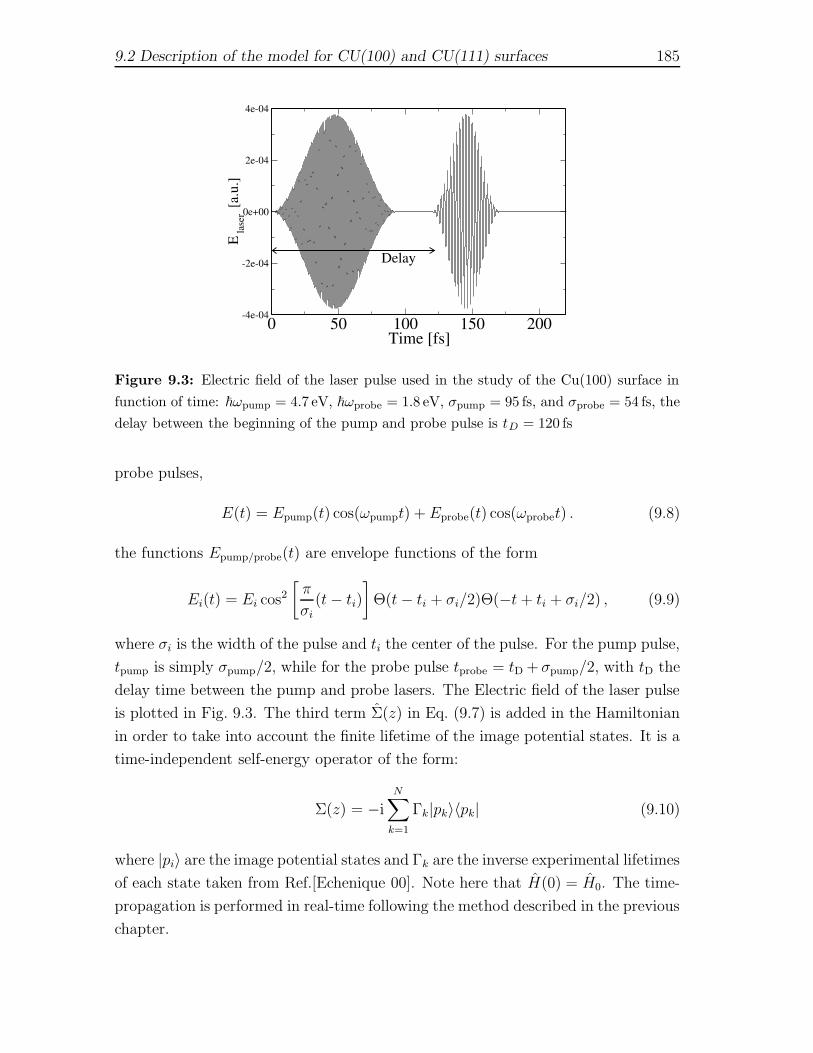
9.2 Description of the model for CU(100) and CU(111) surfaces 185
0 50 100 150 200Time [fs]
-4e-04
-2e-04
0e+00
2e-04
4e-04
E lase
r [a.u
.]
Delay
Figure 9.3: Electric field of the laser pulse used in the study of the Cu(100) surface in
function of time: ~ωpump = 4.7 eV, ~ωprobe = 1.8 eV, σpump = 95 fs, and σprobe = 54 fs, the
delay between the beginning of the pump and probe pulse is tD = 120 fs
probe pulses,
E(t) = Epump(t) cos(ωpumpt) + Eprobe(t) cos(ωprobet) . (9.8)
the functions Epump/probe(t) are envelope functions of the form
Ei(t) = Ei cos2
[
π
σi(t− ti)
]
Θ(t− ti + σi/2)Θ(−t + ti + σi/2) , (9.9)
where σi is the width of the pulse and ti the center of the pulse. For the pump pulse,
tpump is simply σpump/2, while for the probe pulse tprobe = tD + σpump/2, with tD the
delay time between the pump and probe lasers. The Electric field of the laser pulse
is plotted in Fig. 9.3. The third term Σ(z) in Eq. (9.7) is added in the Hamiltonian
in order to take into account the finite lifetime of the image potential states. It is a
time-independent self-energy operator of the form:
Σ(z) = −iN∑
k=1
Γk|pk〉〈pk| (9.10)
where |pi〉 are the image potential states and Γk are the inverse experimental lifetimes
of each state taken from Ref.[Echenique 00]. Note here that H(0) = H0. The time-
propagation is performed in real-time following the method described in the previous
chapter.

186 Chapter 9. Two photon-photoemission spectra of Cu metal surfaces
-400 -200 0 200 400z (a.u.)
0
0.2
0.4
0.6
0.8
1
Mas
k fu
nctio
n
0
0.01
0.02
0.03
0.04
0.05
Den
sity
n1(z)
n2(z)
n3(z)
REGION A
REG
ION
B
REG
ION
B
Figure 9.4: Typical shape of the mask function, M , used for dividing the space in two
regions (see text for details). For illustrative purposes we also plot the densities of the
first three image states of Cu(100).
9.3 Energy-resolved spectra
The energy-resolved photo-electron spectra is obtained following the mask method
technique described in the previous chapter. As explained before we divide the
simulation box in two regions. The region, A, containing the slab and the region
where the first image potential states lie, and another, B, defined as the complement
of A . In region B the electrons are considered free outgoing particles, and are treated
in momentum space. The separation between the two regions is achieved through
a smooth masking function, M , defined as one in the interior of region A and zero
outside (see Fig. 9.4). The method, described in section (8.1.1) consists in evolving
the wave-packet in the region A with the Hamiltonian (9.7), and mask the orbitals at
each time-step. The electrons that “leave” region A are then treated as free-particles
and accumulated in momentum space. Looking at Eq. (8.20) the Energy-resolved
photo-electron spectrum is identified as:
P (√
2mE) =
N∑
k=1
|ψBk (p, t→ ∞)|2 (9.11)
where N is the total number of electrons. In Fig. 9.5 we depict the energy resolved
spectra of a Cu(100) and a Cu(111) surfaces for both zero and finite pump-probe
delay. For the (100) surface, the binding energies of the first image potential states

9.3 Energy-resolved spectra 187
0.5 1 1.5 2 2.5 30
0.5 1 1.5 2 2.5 3Kinetic energy (eV)
0
2PPE
Inte
nsity
(arb
itrar
y un
its)
delay 150fs
delay 0fs
n=1
n=1
n>1
n>1<
<
0.5 1 1.5 2 2.5 30
0.5 1 1.5 2 2.5 3Kinetic energy (eV)
0
2PPE
Inte
nsity
(arb
itrar
y un
its)
delay 55fs
delay 0fs
n=1
n=1
n > 1
n > 1b
2
Figure 9.5: Photo-electron energy resolved spectra of a Cu(100) (left panel) and a
Cu(111) (right panel) surfaces for both zero and finite pump-probe delay.
are -0.57, -0.18, and -0.08 eV (see Fig. 9.1), while for the (111) surface the first states
are at -0.82, -0.22 and -0.009 eV. Note that the second and third image states of the
Cu(111) surface are resonances. Furthermore, the laser parameters used in these
calculations were, for the (100) surface, ~ωpump = 4.7 eV, ~ωprobe = 1.8 eV, σpump =
95 fs, and σprobe = 54 fs, and for the (111) surface, ~ωpump = 5.1 eV, ~ωprobe = 1.8 eV,
σpump = 87 fs, and σprobe = 50 fs. From these results we observe that the peaks
corresponding to the first image potential state are obtained at the correct energy
position. The signal due to the image states of higher quantum number cannot be
distinguished due to the small difference in energy that cannot be resolved with our
grid resolution. We also note that, for zero delay, the broadening of the peak relative
to the first image potential state is larger in the case of the Cu(100) surface than
in the Cu(111). This is due to the fact that in the former case, the probe pulse
can ’pump’ low lying energy electrons from the bulk into energy levels near the gap
which can be then ejected from the surface by the pump pulse. As the Cu(111)
surface has a different electronic structure, such situation does not occur. Note that
Cu(100) shows an intrinsic surface state resonance, while Cu(111) has a surface state

188 Chapter 9. Two photon-photoemission spectra of Cu metal surfaces
0 100 200 300 400 500Time (fs)
0
0.5
1Po
pula
tion
n=1n=2
n=3
Cu(100)ω=4.7eVσ1=85fs
Figure 9.6: Left: Population of the image states p = 1, 2, and 3 as function of time. The
values of Γi=1,2,3 appearing in Eq. (9.10) were taken from Ref. [Echenique 00], and the
maximum of each curve was normalized to one. Right: 2PPE intensity for the p = 1, 2,
and 3 image states of Cu(100) as function of the pump-probe delay. Reproduced from
Ref.[Hofer 97].
below the Fermi level. In the last case, the dominant transition happens between the
occupied surface state and the first image potential state. This can be rationalized
in terms of the larger spacial overlap between surface and image states as compared
to bulk states.
9.4 Time-resolved spectra
The typical energy width of the laser pulses used in TR-2PPE varies between about
10 and 30meV. With this energy resolution it is possible to excite separately each
one of the first three image potential states of Cu(100). By following the TR-
2PPE intensity in function of the pump-probe delay it is then possible to follow the
evolution of the population of these states. In Fig. 9.6 we present calculations of
the populations of the first three image states of Cu(100). The curves were obtained
by propagating the system with the Hamiltonian (9.7) and projecting out the time
dependent wave-function onto the considered image potential states:
Popi(t) = |〈ψimagi |Φ(t)〉|2 (9.12)
For comparison we also show the experimental data from Ref. [Hofer 97]. Clearly,
there is a good qualitative agreement between the theoretical and experimental
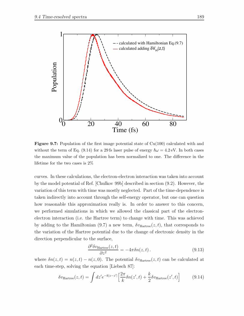
9.4 Time-resolved spectra 189
0 20 40 60 80Time (fs)
0
1
Popu
latio
ncalculated with Hamiltonian Eq.(9.7)calculated adding δVH(z,t)
Figure 9.7: Population of the first image potential state of Cu(100) calculated with and
without the term of Eq. (9.14) for a 29 fs laser pulse of energy ~ω = 4.2 eV. In both cases
the maximum value of the population has been normalized to one. The difference in the
lifetime for the two cases is 2%
curves. In these calculations, the electron-electron interaction was taken into account
by the model potential of Ref. [Chulkov 99b] described in section (9.2). However, the
variation of this term with time was mostly neglected. Part of the time-dependence is
taken indirectly into account through the self-energy operator, but one can question
how reasonable this approximation really is. In order to answer to this concern,
we performed simulations in which we allowed the classical part of the electron-
electron interaction (i.e. the Hartree term) to change with time. This was achieved
by adding to the Hamiltonian (9.7) a new term, δvHartree(z, t), that corresponds to
the variation of the Hartree potential due to the change of electronic density in the
direction perpendicular to the surface,
∂2δvHartree(z, t)
∂z2= −4πδn(z, t) . (9.13)
where δn(z, t) = n(z, t) − n(z, 0). The potential δvHartree(z, t) can be calculated at
each time-step, solving the equation [Liebsch 87]:
δvHartree(z, t) =
∫
dz′e−k|z−z′|[2π
kδn(z′, t) +
k
2δvHartree(z
′, t)]
(9.14)
190 Chapter 9. Two photon-photoemission spectra of Cu metal surfaces
Note that Eq. (9.14) implies Eq. (9.13) regardless of the values of k. Exchange and
correlation effects were treated as before, i.e. through the self-energy term (9.10)
used to simulate the lifetime of the states. The evolution of the population of the
first image state with and without this term is shown in Fig. 9.7. We observe only
a minor shift of the peak to lower times from 24fs to 21.3fs and the lifetime is
reduced by around 2% when the term of Eq. (9.13) is included. This result validates
previous studies that have neglected this effect [Osma 99b, Sarria 99, Chulkov 98,
Chulkov 99a].
In conclusion we have performed dynamical simulations in order to calculate
energy-resolved photo-emission spectra of the Cu(100) and Cu(111) metal surfaces.
We see that the methodology described in chapter (8) gives reliable results for PES.
Using the same technique we also obtained time-resolved photo-emission spectra
for individual excitations of the first three image potential states of Cu(100). This
technique is quite general, and can be used to gain insight on the dynamics of image
states with large quantum number and when more than one eigenstate is excited
coherently (the situation in quantum beat spectroscopy). Furthermore, we have
studied the influence of the variation of the Hartree potential during the excitation.
This effects turn out to be small (around 2%).
A Publications
During the Phd period
• M.A.L. Marques, X. Lopez, D.Varsano, A. Castro and A. Rubio, Time Depen-
dent Density Functional approach to biological chromophore: The case of the
Green Fluorescent Protein Phys. Rev. Lett. 90, 258101 (2003).
• D. Varsano, M.A.L. Marques and A. Rubio, Time and Energy resolved two
photon photoemission of the Cu(100) and Cu(111) metal surfaces Computa-
tional Material Science 30, 110 (2004).
• A. Castro, M.A.L Marques, X. Lopez, D. Varsano and A. Rubio Excited states
properties of nanostructures and biomolecules through time dependent density
functional theory, Proceedings of the 3rd International Conference Computa-
tional Modeling and Simulation of Materials & Special Symposium ”Modeling
and Simulating Materials Nanoworld”, Acireale, Italy, 2004
• R. Di Felice, A. Calzolari, D. Varsano and A. Rubio, Electronic structure
calculations for nanomolecular systems in ”Introducing Molecular Electronics”,
Lecture Notes in Physics Vol.(680), Page.(77-116), (Springer, Berlin, 2005)
• D. Varsano, R. Di Felice, M.A.L. Marques and A. Rubio A TDDFT study
of the excited states of DNA bases and their assemblies Journal of Physical
Chemistry B 110, 7129 (2006)
• C.A. Rozzi, D. Varsano, A. Marini, A. Rubio and E.K.U. Gross An exact
Coulomb cutoff technique for supercell calculations accepted in Physical Review
B (2006)
In Preparation
• D. Varsano, A. Marini and A. Rubio Excitonic properties of quasi-1d systems:
from finite chains to infinite polymers
191

192 Chapter A. Publications
• D. Varsano, A. Marini and A. Rubio Optical spectra and EELS of atomic
chains.
• D. Varsano, M.A.L. Marques, H. Appel, A.Rubio and E.K.U Gross Photo-
electron spectroscopy: a TDDFT approach
• M. Gruening, A. Marini, D. Varsano, L. Wirtz, P. Garcia Gonzalez and A.
Rubio Combining MBPT and TDDFT for static and dynamic properties of
nanosctructures and solids
• D. Varsano, R. Di Felice, M.A.L. Marques and A. Rubio Circular dichroism
within TDDFT of DNA bases and base pairs
Previous publications
• D. Varsano, S. Moroni, G. Senatore, Spin-polarization transition in the two-
dimensional electron gas Europhysics Letters 53 348 (2001)
• G. Senatore, S. Moroni, D. Varsano Spin effects in the 2D electron gas, Solid
State Communications 119, 333 (2001)
• G. Senatore, S. Moroni, D. Varsano, Spontaneous magnetization of the 2D
electron gas, Computer Physics Communications 142, 406 (2001)

Acknowledgments
El Donostia International Physics Center me ha acogido con la mayor simpatıa y
quiero expresar a todos mi reconocimiento, en particular al director Pedro Miguel
Echenique, no solamente por las discusiones cientificas que hemos tenido durante
mi primer ano de doctorado, sino tambien por la sensibilidad que ha sabido de-
mostrarme durante toda mi permanencia en el DIPC.
Quiero agradecer a mi director de tesis Angel Rubio, por todo lo que me ha ensenado
y por haberme hecho de guıa en este trabajo durante cuatro anos. Este trabajo
no hubiera sido posible sin sus consejos. Together with Angel I want to thank
all the group for the discussions and the time spent together: Alberto, Ludger,
Miguel, Myrta, Andrea and Francesco. Quiero agradecer a Pablo Garcıa-Gonzalez
por haberme animado en el trabajo cada vez hemos coincidido, en Donostia y en las
conferencias, y ademas por haberme corregido el castellano la unica (y ultima) vez
que he intentado escribir algo en este idioma.
I would like to thank all those who I have collaborated with: the group of Elisa Moli-
nari at the Univeristy of Modena that have been very nice with me each time I spent
time there. In particular I’m indebted to Rosa Di Felice not only for examining the
thesis but also for several discussion and suggestion during our collaboration. The
group of Rodolfo Del Sole of the University of Rome “Tor Vergata” for their hospi-
tality during the last period of my work, and in particular to Andrea Marini, former
member of Angel’s group, for discussing, collaborating and mainly teach me a lot
about physics and coding, and also to Olivia Pulci for carefully reading this work.
The group of Hardy Gross for inviting me in Wuerzburg at the very beginning of
the thesis, and it has been a pleasure to work and discuss with Carlo Andrea Rozzi
and Heiko Appel. Y quiero agradecer mucho a los quımicos Xabier Lopez y Eider
Sansebastian por su disponibilidad y por los calculos de estructuras de moleculas
biologicas.
Los anos pasados aqui en Donostia no hubieran sido los mismos sin los companeros
de despacho y verdaderos amigos: Aitor, Aran, Asier eta Maider, eskerrik asko lagu-
nak. No podrıa no agradecer a Miguel y Daniele, entre muchas otras cosas, por sus
hospidalidad en estos ultimos dıas en Donosti en que me encuentro escribiendo estas
lıneas. Agradezco mucho a Txomin, Belen y Tomas siempre disponibles a resolver
193

194 Chapter A. Publications
cualquier problema.
This work would have not been possible without the financial support from the net-
work of the European Community: Nanoquanta, Comelcan and DNA-Nanowires.
Per finire ringrazio sinceramente Stef, per avermi sopportato e ospitato in piu occa-
sioni durante l’ultimo periodo di questo lavoro.
Ai miei genitori devo tutta la mia gratitudine e affetto per l’aiuto e l’incorraggiamento
ricevuto in questi anni nonostante la distanza.
Daniele
March 2006

Bibliography
[Adler 62] S. L. Adler. Phys. Rev, 126, 413, 1962.
[Adragna 03] G. Adragna, R. Del Sole and A. Marini. Phys. Rev. B , 68,
165108, 2003.
[Agostini 79] P. Agostini, F. Fabre, G. Mainfray, G. Petite and N.K. Rah-
man. Phys. Rev. Lett. , 42, 1127, 1979.
[Albrecht 98] S. Albrecht, L. Reining, R. Del Sole and G.Onida. Phys. Rev.
Lett. , 80, 4510, 1998.
[Albrecht 99] S. Albrecht. PhD thesis, Ecole Polytechnique, 1999.
[Almbladh 83] C. O. Almbladh and L. Hedin. Handbook on synchrotron ra-
diation, volume 1, . North-Holland, New York, 1983.
[Almbladh 85] C. O. Almbladh and U. Von Barth. Phys. Rev. B , 31, 3231,
1985.
[Appel 03] H. Appel, E. K. U. Gross and K.Burke. Phys. Rev. Lett. , 90,
43005, 2003.
[Arnott 72] S. Arnott and D. W. L. Hukins. Biochem. Biophys. Res. Com-
mun., 47, 1504, 1972.
[Arnott 74] S. Arnott and E. Selsing. J. Mol. Biol, 88, 509, 1974.
[Aryasetiawan 98] F. Aryasetiawan and O. Gunnarson. Rep. Prog. Phys., 61, 237,
1998.
[Aulbur 00a] W. G. Aulbur, L. Jonsson and J. W. Wilkins. Solid state phys.,
volume 54, . Academic, Orlando, 2000.
[Aulbur 00b] W. G. Aulbur, M. Stadele and A. Gorling. Phys. Rev. B , 62,
7121, 2000.
[Baer 05] R. Baer and D. Neuhauser. Phys. Rev. Lett. , 94, 43002, 2005.
195
196 Bibliography
[Bandrau 03] D. Bandrau and I. Kawata S. Chelkowski. Phys. Rev. A, 67,
013407, 2003.
[Bauer 01] D. Bauer and F. Ceccherini. Optic Express, 8, 377, 2001.
[Baym 62] G. Baym and L. Cadanoff. Quantum statistical mechanics.
W.A.Benjamin Inc, New York, 1962.
[Beck 00] T. L. Beck. Rev. Mod. Phys. , 72, 1041, 2000.
[Becke 88] A. D. Becke. Phys. Rev. A , 38, 3090, 1988.
[Bell 00] A. Bell, X. He, R. M. Wachter and P. J. Tonge. Biochemistry,
39, 4423, 2000.
[Benedict 98] L. X. Benedict, E.L. Shirley and R.B. Bohn. Phys. Rev. Lett.
, 80, 4514, 1998.
[Berger 05] J. A. Berger, P. L. de Boeij and R. van Leeuwen. J. Chem.
Phys., 123, 174910, 2005.
[Bowler 00] D. R. Bowler and M. J. Gillan. Chem. Phys. Lett., 325, 473,
2000.
[Brabec 00] T. Brabec and F. Krausz. Rev. Mod. Phys. , 72, 545, 2000.
[Brealey 55] G. Brealey and M. Kasha. J. Am. Chem. Soc., 77, 4462, 1955.
[Brejc 97] K. Brejc, T.K. Sixma, P.A. Kitts, S.R. Kain, R.Y. Tsien,
M. Ormo and S.J. Remington. Proc. Natl. Acad. Sci. U.S.A.,
94, 2306, 1997.
[Brodka 03] A. Brodka. Mol. Phys., B 61, 3177, 2003.
[Broo 98] A. Broo. J. Phys. Chem. A, 102, 526, 1998.
[Brooks 83] B. R. Brooks et al. J. Comput. Chem., 2, 148, 1983.
[Brunger 88] A. T. Brunger and M. Karplus. Proteins, 4, 148, 1988.
[Brunner 75] W. C. Brunner and M. F. Maestre. Biopolymers, 14, 555, 1975.

Bibliography 197
[Burke 02] K. Burke, M.Petersilka and E. K. U. Gross. Recent advances in
densuty functional methods, 67. World Scientific, Singapore,
2002.
[Callis 64] P. R. Callis, E. J. Rosa and W. T. Simpson. J. Am. Chem.
Soc., 86, 2292, 1964.
[Callis 83] P. R. Callis. Annu. Rev. Phys. Chem., 37, 691, 1983.
[Calzolari 04a] A. Calzolari, R. Di Felice, E. Molinari and A. Garbesi. J. Phys.
Chem. B, 108, 2509, 2004.
[Calzolari 04b] A. Calzolari, R. Di Felice, E. Molinari and A. Garbesi. J. Phys.
Chem. B, 108, 13058, 2004.
[Casida 95] E. Casida. Recent advances in density functionals methods,
volume 1, . World Scientific, Singapore, 1995.
[Castro 02] A. Castro, M. A. L. Marques, J. A. Alonso, G.F. bertsch,
K. Yabana and A. Rubio. J. Chem. Phys., 116, 1930, 2002.
[Castro 03] A. Castro, A. Rubio and M.J. Stott. Can. J. Phys., 81, 1,
2003.
[Castro 04a] A. Castro. PhD thesis, Universidad de Valladolid, 2004.
[Castro 04b] A. Castro, M. A. L. Marques, J. A. Alonso, G. F. Bertsch and
A. Rubio. European Journal of Physics D, 28, 211, 2004.
[Castro 04c] A. Castro, M. A. L. Marques and A. Rubio. J. Chem. Phys.,
121, 3425, 2004.
[Ceperley 80] D.M. Ceperley and B.J. Alder. Phys. Rev. Lett., 45, 566, 1980.
[Champagne 95a] B. Champagne, D. H. Mosley, M. Vracko and J. M. Andre.
Phys. Rev. A , 52, 1039, 1995.
[Champagne 95b] B. Champagne, D. H. Mosley, M. Vracko and J. M. Andre.
Phys. Rev. A , 52, 178, 1995.
[Chulkov 97] E. V. Chulkov, V.M. Silkin and P.M. Echenique. Surf. Sci. ,
391, L1217, 1997.

198 Bibliography
[Chulkov 98] E. V. Chulkov, I. Sarria, V.M. Silkin, J.M. Pitarke and P.M.
Echenique. Phys. Rev. Lett. , 80, 4947, 1998.
[Chulkov 99a] E. V. Chulkov, J. Osma, I. Sarria, V. M. Silkin and J. M.
Pitarke. Surf. Sci. , 433, 882, 1999.
[Chulkov 99b] E. V. Chulkov, V.M. Silkin and P.M. Echenique. Surf. Sci. ,
330, 437, 1999.
[Cinelli 01] R. A. Cinelli, V. Tozzini, V. Pellegrini, F. Beltram, G. Cerullo,
M. Zavelani-Rossi, S. De Silvestri, M. Tyagi and M. Giacca.
Phys. Rev. Lett. , 86, 3439, 2001.
[Clark 65] L. B. Clark and I. Tinoco. J. Am. Chem. Soc., 87, 11, 1965.
[Clark 95] L. B Clark. J. Phys. Chem., 99, 4466, 1995.
[Coehn 05] H. Coehn, C. Nogues, R. Naaman and D. Porath. Proc. Natl.
Acad. Sci. U.S.A., 102, 11589, 2005.
[Cohen 82] M. L Cohen. Phys. Scri., 1, 5, 1982.
[Cohen 94] M. L Cohen. Solid Stat. Comm., 92, 45, 1994.
[Creemers 99] T. M. H. Creemers, A.J. Lock, v. Subramaniam, T.M. Jovin
and S. Volker. Nat. Struc. Biol, 6, 557, 1999.
[Creemers 00] T. M. H. Creemers, A.J. Lock, v. Subramaniam, T.M. Jovin
and S. Volker. Proc. Natl. Acad. Sci. U.S.A., 97, 2974, 2000.
[Daniels 76] M. Daniels. Photochemistry and photobiology of nucleic acids,
volume 1, , 23. Academic Press, New York, 1976.
[de Andres 87] P.L. de Andres, P.M. Echenique and F. Flores. Phys. Rev. B ,
35, 4529, 1987.
[de Andres 89] P.L. de Andres, P.M. Echenique and F. Flores. Phys. Rev. B ,
39, 10356, 1989.
[Dederichs 83] P. H. Dederichs and R. Zeller. Phys. Rev. B , 28, 5462, 1983.
[DeLeeuw 80] S. W. DeLeeuw, J. W. Perram and E. R. Smith. Proc. R. Soc.
Lond., A 373, 27, 1980.
Bibliography 199
[Delerue 03] C. Delerue, M. Lannoo and G.Allan. Phys. Rev. Lett. , 90,
076803, 2003.
[Dewar 95] M. J. S. Dewar, E. Zoebisch, E.F. Healy and J.J.P. Stewart. J.
Am. Chem. Soc., 107, 3902, 1995.
[Di Felice 02] R. Di Felice, A. Calzolari, E. Molinari and A. Garbesi. Phys.
Rev. B , 65, 045104, 2002.
[Di Felice 05] R. Di Felice and A.Calzolari. Modern methods for theoretical
physical chemestry of biopolymers. Elsevier, 2005.
[Dreizler 90] R. M. Dreizler and E. K. U. Gross. Density functional theory,
an approach to the quantum many body problem. Springer
Verlag, Berlin, 1990.
[Dreuw 03] A. Dreuw, J. L. Weisman and M. Head-Gordon. J. Chem.
Phys., 119, 2943, 2003.
[Dreuw 04] A. Dreuw, J. L. Weisman and M. Head-Gordon. J. Am. Chem.
Soc., 126, 4007, 2004.
[Eaton 70] W. A. Eaton and T. P. Lewis. J. Chem. Phys., 53, 2164, 1970.
[Eberly 91] J. H. Eberly, J. Javanainen and K. Rzazewsky. Phys. Rep, 204,
331, 1991.
[Echenique 78] P. M. Echenique and J.B. Pendry. J. Phys. C, 11, 2065, 1978.
[Echenique 90] P. M. Echenique and J.B. Pendry. Prog. Surf. Sci., 32, 111,
1990.
[Echenique 00] P. M. Echenique, J.M. Pitarke, E.V. Chulkov and A. Rubio.
Chem. Phys., 251, 1, 2000.
[Echenique 02] P. M. Echenique, J.M. Pitarke, E.V. Chulkov and V.M. Silkin.
J. Elect. Spect., 126, 165, 2002.
[Endres 04] R. G. Endres, D.L. Cox and R.R.P. Singh. Rev. Mod. Phys. ,
76, 195, 2004.
[Ewald 21] P. P. Ewald. Ann. Phys., 64, 253, 1921.

200 Bibliography
[Faisal 87] F.H.M. Faisal. Theory of multiphoton processes. Plenum, New
York, 1987.
[Fauster 95] Th. Fauster and W. Steinmann. Photonic probes of surfaces,
volume 2, . Elsevier, Amsterdam, 1995.
[Feit 82] M. D. Feit, J. A. Fleck and A. Steiger. J. Comput. Phys., 47,
412, 1982.
[Fermi 28] E. Fermi. Z. Phys, 48, 73, 1928.
[Fetter 81] L. Fetter and J. D.Walecka. Quantum theory of many-body
systems. McGraw Hill, New York, 1981.
[Field 90] M. J. Field, P. A. Bash and M. Karplus. J. Comp. Chem., 11,
700, 1990.
[Fiolhais 03] C. Fiolhais, F. Nogueira and M. A. L. Marques, editors. A
primer in density functional theory. Springer, Berlin, 2003.
[Flocard 78] H. Flocard, S. E. Koonin and M. S. Weiss. Physical Review C,
17, 1682, 1978.
[Fock 30] V. Fock. Z. Phys, 61, 126, 1930.
[Fornberg 94] B. Fornberg and D. M. Sloan. Acta numerica 1994, 203–267.
Cambridge University Press, Cambridge, 1994.
[Frigo 98] M. Frigo and S.G Johnson. Proc. IEEE Int. Conf. Acoust.
Speech, Signal Processing, ICASSP’98, 3, 1381, 1998.
[Fucaloro 71] A. F. Fucaloro and L. S. Forster. J. Am. Chem. Soc., 93, 6443,
1971.
[Fulscher 95] M. P. Fulscher and B. Roos. J. Am. Chem. Soc., 117, 2089,
1995.
[Fulscher 97] M. P. Fulscher, L. Serrano-Andres and B. Roos. J. Am. Chem.
Soc., 119, 6168, 1997.
[Furche 05] F. Furche and K. Burke. Ann. Rev. Comp. Chem., 1, 19, 2005.

Bibliography 201
[Gao 99] Y. G Gao, H. Robinson and A. H. Wang. Eur. J. Biochem.,
261, 413, 1999.
[Ghosez 97] P. Ghosez, X. Gonze and R. W. Godby. Phys. Rev. B , 56,
12811, 1997.
[Giesen 85] K. Giesen, F. Hage, F.J. Himpsel, H.J. Riess and W. Stein-
mann. Phys. Rev. Lett. , 55, 300, 1985.
[Godby 86] R. W. Godby, M. Schluter and L.J. Sham. Phys. Rev. Lett. ,
56, 2415, 1986.
[Godby 87a] R. W. Godby, M. Schluter and L.J. Sham. Phys. Rev. B , 36,
3497, 1987.
[Godby 87b] R. W. Godby, M. Schluter and L.J. Sham. Phys. Rev. B , 35,
4170, 1987.
[Godby 88] R. W. Godby, M. Schluter and L.J. Sham. Phys. Rev. B , 37,
10159, 1988.
[Godby 89] R. W. Godby and R. J. Needs. Phys. Rev. Lett. , 62, 1169,
1989.
[Godby 90] R. W. Godby, L.J. Sham and M. Schluter. Phys. Rev. Lett. ,
65, 2083, 1990.
[Godby 94] R. W. Godby and L.J. Sham. Phys. Rev. B , 49, 1849, 1994.
[Goedecker 96] S. Goedecker, M. Teter and J. Huetter. Phys. Rev. B , 54,
1703, 1996.
[Gonze 95] X. Gonze, P. Ghosez and R. W. Godby. Phys. Rev. Lett. , 74,
4035, 1995.
[Gonze 97a] X. Gonze, P. Ghosez and R. W. Godby. Phys. Rev. Lett. , 78,
294, 1997.
[Gonze 97b] X. Gonze, P. Ghosez and R. W. Godby. Phys. Rev. Lett. , 78,
2029, 1997.
[Gonze 99] X. Gonze and M. Scheffler. Phys. Rev. Lett. , 82, 4416, 1999.
202 Bibliography
[Gonze 05] X. Gonze, G. M. Rignanese, M. Versraete et al. Zeit. Kristal-
logr., 220, 558, 2005.
[Granville 81] M. F. Granville, B. E. Kohler and J. Bannon Snow. J. Chem.
Phys., 75, 3765, 1981.
[Greengard 88] L. Greengard. The rapid evaluation of potential fields in par-
ticle system. MIT press, Cambridge, 1988.
[Grimee 03] S. Grimee and M. Parac. ChemPhysChem, 4, 292, 2003.
[Gritsenko 01] O. V. Gritsenko and E. J. Baerends. Phys. Rev. A , 64, 42506,
2001.
[Gritsenko 04] O. V. Gritsenko and E. J. Baerends. J. Chem. Phys., 121, 655,
2004.
[Grobe 93] R. Grobe and J. H. Eberly. Phys. Rev. A, 48, 4664, 1993.
[Gross 91] E. K. U. Gross, E. Runge and O. Heinonen. Many-particle
theory. Adam-Hilger, Bristol, 1991.
[Gross 95] E. K. U. Gross, C.A. Ullrich and U.J. Gossman. Density func-
tional theory, volume 337, . NATO ASI Ser. B Plenum Press,
New York, 1995.
[Gross 96] E. K. U. Gross, J. F. Dobson and M. Petersilka. Density func-
tional theory ii, topics in current chemistry. Springer Verlag,
Berlin, 1996.
[Grosso 00] G. Grosso and G. Pastori Parravicini. Solid state physics. Aca-
demic Press, San Diego, 2000.
[Gruning 02] M. Gruning, O. Gritsenko and E. Baerends. J. Chem. Phys.,
116, 6435, 2002.
[Grzybowski 00] A. Grzybowski, E. Gwozdz and A. Brodka. Phys. Rev. B , 61,
6706, 2000.
[Haight 95] R. Haight. Surf. Sci. Rep., 8, 275, 1995.
[Hall 96] D. B. Hall, R. E. Holmlin and J. K. Barton. Nature, 3841, 731,
1996.
Bibliography 203
[Hanke 80] W. Hanke and L. J. Sham. Phys. Rev. B , 21, 4656, 1980.
[Hartree 28] D. R. Hartree. Proc. Cambridge Philos. Soc., 24, 89, 1928.
[Haupts 98] U. Haupts, S. Maiti, P. Schwille and W.W. Webb. Proc. Natl.
Acad. Sci. U.S.A., 95, 13573, 1998.
[Hedin 65] L. Hedin. Phys. Rev, 139, 796, 1965.
[Hedin 69] L. Hedin and S. Lundqvist. Solid State Phys., 23, 1, 1969.
[Hedin 71] L. Hedin and B. I. Lundqviust. J. Phys. C, 4, 2064, 1971.
[Heeger 88] A. J. Heeger, S. Kivelson, J. R. Schrieffer and W. P. Su. Rev.
Mod. Phys. , 60, 781, 1988.
[Helms 00] V. Helms, C. Winstead and P. W. Langhoff. J. Mol. Struc.
(Thoechem, 506, 179, 2000.
[Hernandez 04a] C. E. Crespo Hernandez, B. Cohen, P. M. Hare and B. Kohler.
Chem. Rev., 104, 1977, 2004.
[Hernandez 04b] C. E. Crespo Hernandez, C. Marai and B. Kohler. unpublished,
2004.
[Hernandez 05] C. E. Crespo Hernandez, B. Kohler and B. Cohen. Nature,
436, 1141, 2005.
[Heyes 77] D.M. Heyes, M. Barber and J.H.R. Clarke. J. Chem. Soc.
Faraday Trans II, 73, 1485, 1977.
[Hofer 97] U. Hofer, I.L. Shumay, Ch. Reuß, U. Thomann, W. Wallauer
and Th. Fauster. Science, 277, 1480, 1997.
[Hohenberg 64] P. Hohenberg and W. Kohn. Phys. Rev., 136, B864, 1964.
[Holmen 97] A. Holmen, A. Broo, B. Albinsson and B. Norden. J. Am.
Chem. Soc., 119, 12240, 1997.
[Hutchinson 03] G. R. Hutchinson, Y. Zhao, B. Delley, A. J. Freeman, M. A.
Ratner and T. J.Marks. Phys. Rev. B , 68, 35204, 2003.

204 Bibliography
[Hybertsen 85] M. S. Hybertsen and S. G. Louie. Phys. Rev. Lett. , 55, 1418,
1985.
[Hybertsen 86] M. S. Hybertsen and S. G. Louie. Phys. Rev. B , 34, 5390,
1986.
[Hybertsen 88] M. S. Hybertsen and S. G. Louie. Phys. Rev. B , 37, 10159,
1988.
[I.S. Gradshteyn 80] M. Rhysik I.S. Gradshteyn. Tables of integrals, series and prod-
ucts. Academic, New York, 1980.
[Ismail 02] N. Ismail, L. Blancafort, M. Olivucci, B. Kohler and M. A.
Robb. J. Am. Chem. Soc., 87, 6818, 2002.
[Jackson 75] J. D. Jackson. Classical electrodynamics. Wiley and Sons, New
York, 1975.
[Jamorsky 96] C. Jamorsky, M. E. Casida and D. R. Salahub. J. Chem. Phys.,
104, 5134, 1996.
[Jarvis 97] M. R. Jarvis, I. D. White, R. W. Godby and M. C. Payne.
Phys. Rev. B , 56, 14072, 1997.
[Jean 01] J. M. Jean and K. B Hall. Proc. Natl. Acad. Sci. U.S.A., 98,
37, 2001.
[Jean 02] J. M. Jean and K. B Hall. Biochemistry, 41, 13152, 2002.
[Johnson 88] D. D. Johnson. Phys. Rev. B , 38, 12807, 1988.
[Jones 89] R. O. Jones and O. Gunnarson. Rev. Mod. Phys. , 61, 689,
1989.
[Jortner 98] J. Jortner, M. Bixon, T. Lagenbacher and M. E. Michel-
Bayerle. Proc. Natl. Acad. Sci. U.S.A., 95, 12759, 1998.
[Kim 00] N. J. Kim, G. Jeong, Y. S. Kim, J. Sung, S. K. Kim and
Y. Park. J. Chem. Phys., 113, 10051, 2000.
[Kim 02a] Y. H. Kim and A. Gorling. Phys. Rev. Lett. , 89, 96402, 2002.
[Kim 02b] Y. H. Kim and A. Gorling. Phys. Rev. B , 66, 35114, 2002.
Bibliography 205
[Kirtman 95] B. Kirtman, J. L. Toto, K. A. Robins and M. Hasan. J. Chem.
Phys., 102, 5350, 1995.
[Klamroth 01] T. Klamroth, P. Saalfrank and U. Hofer. Phys. Rev. B , 64,
035420, 2001.
[Kleiman 82] L. Kleiman and D. M. Bylander. Phys. Rev. Lett. , 48, 1425,
1982.
[Kohn 65] W. Kohn and L.J. Sham. Phys. Rev., 140, A1133, 1965.
[Kohn 99] W. Kohn. Rev. Mod. Phys. , 71, 1253, 1999.
[Kraemer 97] K. H. Kraemer. Proc. Natl. Acad. Sci. U.S.A., 94, 11, 1997.
[Kreibich 01] T. Kreibich and E. K .U Gross. Phys. Rev. Lett. , 86, 2984,
2001.
[Krieger 90] J. B. Krieger, Y.Li and G. J. Iafrate. Phys. Letters A, 146,
256, 1990.
[Krieger 92] J. B. Krieger, Y.Li and G. J. Iafrate. Physical Review A, 45,
101, 1992.
[Kudin 04] K. N. Kudin and G. E Scuseria. J. Chem. Phys., 121, 2886,
2004.
[Kummel 04] S. Kummel, L. Kronik and J. P. Perdew. Phys. Rev. Lett. ,
93, 213002, 2004.
[Laio 02] A. Laio, J. VandeVondele and U. Rothlisberger. J. Chem.
Phys., 116, 6941, 2002.
[Lappas 98] D.G. Lappas and R. van Leeuwen. Journal of Physics B, 31,
L245, 1998.
[Lee 88] C. Lee, W. Yang and R. G. Parr. Phys. Rev. B , 37, 785, 1988.
[Lein 01] M. Lein, E. K. U. Gross and V. Engel. Phys. Rev. A, 64,
023406, 2001.
[Leising 88] G. Leising. Phys. Rev. B , 38, 10313, 1988.

206 Bibliography
[Levy 79] M. Levy. Proc. Natl. Acad. Sci. U.S.A., 76, 6062, 1979.
[Levy 84] M. Levy, J.P. Perdew and V. Sahni. Phys. Rev. A , 30, 2745,
1984.
[Lieb 82] E. H. Lieb. Int. J. Quantum Chem., 24, 243, 1982.
[Liebsch 87] A. Liebsch. Phys. Rev. B , 36, 7378, 1987.
[Liegner 85] C. M. Liegner. J. Phys C, 18, 6011, 1985.
[Lopez 05] X. Lopez, M. A. L. Marques, A. Castro and A. Rubio. J. Am.
Chem. Soc., 127, 12329, 2005.
[Lorentzon 95] J. Lorentzon, M. P. Fulscher and B. Roos. J. Am. Chem. Soc.,
117, 9265, 1995.
[Luders 05] M. Luders, M. A. L Marques, N. N Lathiotajis, A. Floris,
G. Profeta, L. Fast, A. Continenza, S. Massidda and E. K .U
Gross. Phys. Rev. B , 72, 24545, 2005.
[Lundqvist 83] S. Lundqvist and N.H. March, editors. Theory of the inhomo-
geneous electron gas. Plenuim Press, New York, 1983.
[MacKerrel 98] A. D. MacKerrel et al. J. Phys. Chem. B, 102, 3586, 1998.
[Maitra 01] N. T. Maitra, K. Burke, H. Appel, E.K.U. Gross and R. van
Leeuwen. Reviews of modern quantum chemistry. World Sci-
entific, New Jersey, 2001.
[Makov 95] G. Makov and M. C. Payne. Phys. Rev. B , 51, 4014, 1995.
[Marini 03] A. Marini, R. Del Sole and A. Rubio. Phys. Rev. Lett. , 91,
2564021, 2003.
[Marini 04] A. Marini and A. Rubio. Phys. Rev. B (Rap. Comm.), 70,
81103, 2004.
[Marques 01] M. A. L. Marques, A. Castro and A. Rubio. J. Chem Phys.,
115, 3006, 2001.
[Marques 03a] M. A. L. Marques, A. Castro, G. F. Bertsch and A. Rubio.
Computer Phys. Commun., 151, 60, 2003.

Bibliography 207
[Marques 03b] M. A. L. Marques, X. Lopez, D.Varsano, A. Castro and A. Ru-
bio. Phys. Rev. Lett. , 90, 258101, 2003.
[Marques 04] M. A. L Marques and E. K. U. Gross. Annu. Rev. Phys. Chem.,
5, 427, 2004.
[Marques 05] M. A. L Marques, M. Luders, N. N Lathiotajis, G. Profeta,
A. Floris, L. Fast, A. Continenza, E. K .U Gross and S. Mas-
sidda. Phys. Rev. B , 72, 24546, 2005.
[Marques 06] M.A.L. Marques, K. Burke, E.K.U. Gross, F. Nogueira, A. Ru-
bio and C. Ullrich, editors. Time dependent density functional
theory: Prospect and apllications. Springer Lecture Notes,
2006.
[Martinez 04] I. Martinez, A. Castro, A. Rubio, J. M. Poblet and J. A.
Alonso. Chemical Physics Letters, 398, 292, 2004.
[Martyna 99] G. J. Martyna and M. E. Tuckerman. J. Chem. Phys., 110,
2810, 1999.
[McNeil 97] J.D. McNeil, R.L. Lingle Jr., N.H. Ge, C.M. Wong and
C.B. Harris R.E. Jordan. Phys. Rev. Lett. , 79, 4645, 1997.
[Mearns 87] D. Mearns and W. Kohn. Phys. Rev. A , 35, 4796, 1987.
[Mennucci 01] B. Mennucci, A. Tonniolo and J. Tommasi. J. Phys. Chem. A,
105, 4749, 2001.
[Merchan 03] M. Merchan and L. Serrano-Andres. J. Am. Chem. Soc., 125,
8108, 2003.
[Miles 67] D. W. Miles, R. K. Robins and K. Eyring. Proc. Natl. Acad.
Sci. U.S.A., 57, 1139, 1967.
[Minary 02] P. Minary, M.E. Tuckerman, K.A. Pihakari and G.J. Martyna.
J. Chem. Phys., 116, 5351, 2002.
[Minary 04] P. Minary, J.A. Morrone, D.A. Yarne, M.E. Tuckerman and
G.J. martina. J. Chem. Phys., 121, 11949, 2004.

208 Bibliography
[Mishra 00] S. K. Mishra, M. K. Shukla and P. C. Mishra. Spectrochim.
Acta Part A, 56, 1355, 2000.
[Mons 02] M. Mons, I. Dimicoli, F.Piuzzi, B. Tardivel and M. Elhanine.
J. Phys. Chem. A, 106, 5088, 2002.
[Nalwa 05] H. S. Nalwa, editor. Encyclopedia of nanoscience and nan-
otechnology and hndbook of nanostructured biomaterials and
their application in nanotechnology. APS, 2005.
[Neiss 03] C. Neiss, P. Saalfrank, M. Parac and S. Grimme. J. Phys.
Chem. A, 107, 140, 2003.
[Nielsen 01] S. B. Nielsen, A. Lapierre, J.U. Andersen, U.V. Pedersen,
S. Tomita and L.H. Andersen. Phys. Rev. Lett. , 87, 228102,
2001.
[Nir 02] E. Nir et al. Chem. Phys. Lett., 59, 355, 2002.
[Odom 01] D. T. Odom and J. K. Barton. Biochemistry, 40, 8727, 2001.
[Onida 95] G. Onida, L. Reining, R. W. Godby, R. Del Sole and W. An-
dreoni. Phys. Rev. Lett. , 75, 818, 1995.
[Onida 02] G. Onida, L. Reining and A. Rubio. Rev. Mod. Phys. , 74,
601, 2002.
[Osma 99a] J. Osma. PhD thesis, Universidad del Paıs Vasco, 1999.
[Osma 99b] J. Osma, I. Sarria, E.V. Chulkov, J.M. Pitarke and P.M.
Echenique. Phys. Rev. B , 59, 10591, 1999.
[Payne 92] M. C. Payne, M. P. Teter, D. C. Allan, T. A. Arias and J. D.
Joannopoulo. Rev. Mod. Phys. , 64, 1045, 1992.
[Perdew 81] J. Perdew and A. Zunger. Phys. Rev. B, 23, 5048, 1981.
[Perdew 92] J. P. Perdew and Y. Wang. Phys. Rev. B , 45, 13244, 1992.
[Perdew 96] J. P. Perdew, K. Burke and M. Ernzerhof. Phys. Rev. Lett. ,
77, 3865, 1996.
Bibliography 209
[Perdew 99] J. P. Perdew, S. Kurth, A. Zupan and P. Blaha. Phys. Rev.
Lett. , 82, 2544, 1999.
[Petek 00] H. Petek, editor. Chem. phys. special issues: Electgron dy-
namics in metals, volume 251, . 2000.
[Petersilka 96] M. Petersilka, U. G. Gossmann and E. K. U. Gross. Phys. Rev.
Lett. , 76, 1212, 1996.
[Petersilka 99] M. Petersilka and E.K.U. Gross. Laser Physics, 9, 105, 1999.
[Pickett 89] W. E. Pickett. Comput. Phys. Rep., 9, 115, 1989.
[Pohl 00] A. Pohl, P. G. Reinhard and E. Suraud. Phys. Rev. Lett. , 84,
5090, 2000.
[Porath 04] D. Porath, G. Cuniberti and R. Di Felice. Topics in current
chemistry, volume 237, , 183. Springer Verlag, Heidelberg,
Germany, 2004.
[Press 92] W. H. Press et al. Numerical recipies, Chap. 2. Cambridge
University Press, Cambridge, 1992.
[Protopapas 97] M. Protopapas, C. H. Keitel and P. L. Knight. Rep. Prog.
Phys., 60, 389, 1997.
[Pulci 06] O. Pulci et al. 2006. to be published.
[Puschnig 03] P. Puschnig and C. Ambrosch Draxl. Synthetic Metals, 135
and 136, 415, 2003.
[Reuter 00] N. Reuter, A. Dejaegere, B. Maigret and M. Karplus. J. Phys.
Chem. A, 104, 1720, 2000.
[Rohlfing 98] M. Rohlfing and S. J Louie. Phys. Rev. Lett. , 81, 2312, 1998.
[Rohlfing 99] M. Rohlfing and S. J Louie. Phys. Rev. Lett. , 82, 1959, 1999.
[Rohlfing 00] M. Rohlfing and S. J Louie. Phys. Rev. B , 62, 4927, 2000.
[Rohlfing 04] M. Rohlfing and S. J Louie. Phys. Rev. B , 70, 193204, 2004.
210 Bibliography
[Rubio 93] A. Rubio, J.L. Corkill, M. L. Cohen, E. Shirley and S. Luoie.
Phys. Rev. B , 48, 11810, 1993.
[Runge 84] E. Runge and E. K. U. Gross. Phys. Rev. Lett. , 52, 997, 1984.
[Ruzsicska 95] B. P. Ruzsicska and D. G. E. Lemaire. Crc handbook of pho-
tochemistry and photobiology, 1289. CRC Press, Boca Raton,
Fl, 1995.
[Sanchez 03] P. Mori Sanchez and Q. Wu adn W. Yang. J. Chem. Phys.,
119, 11001, 2003.
[Sarria 99] I. Sarria, J. Osma, E.V. Chulkov, J.M. Pitarke and P.M.
Echenique. Phys. Rev. B , 60, 11795, 1999.
[Schafer 91] K. J. Schafer and K. C. Kulander. Phys. Rev. A, 42, 5794,
1991.
[Schattke 03] W. Schattke and M. A. Van Hove, editors. Solid-state photoe-
mission and related methods: Theory and experiment. Wiley-
VCH, Berlin, 2003.
[Schoenlein 88] R.W. Schoenlein, J.G. Fujimoto, G.L. Eesley and T.W. Cape-
hart. Phys. Rev. Lett. , 61, 2596, 1988.
[Schoenlein 90] R.W. Schoenlein, J.G. Fujimoto, G.L. Eesley and T.W. Cape-
hart. Phys. Rev. B , 41, 5436, 1990.
[Schuppler 92] S. Schuppler, N. Fischer, Th. Fauster and W. Steinmann. Phys.
Rev. B , 46, 13539, 1992.
[Schwille 00] P. Schwille, S. Kummer, A. A. Heikal, W.E. Moerner and W.W
Webb. Proc. Natl. Acad. Sci. U.S.A., 97, 151, 2000.
[Seminario 96] J. M. Seminario, editor. Recent developments and applications
of modern density functional theory. Elsevier, Amsterdam,
1996.
[Sharp 53] R. T. Sharp and G.!K. Horton. Phys. Rev., 90, 317, 1953.
[Shockley 39] W. Shockley. Phys. Rev., 56, 317, 1939.

Bibliography 211
[Shukla 99] M. K. Shukla and S. K. Mishra. Chem. Phys., 240, 319, 1999.
[Shukla 00] M. K. Shukla, S. K. Mishra, A. Kumar and P. C. Mishra. J.
Comput. Chem., 21, 826, 2000.
[Shukla 02a] M. K. Shukla and J. Leszczynski. J. Phys. Chem. A, 106, 4709,
2002.
[Shukla 02b] M. K. Shukla and J. Leszczynski. J. Phys. Chem. A, 106,
11338, 2002.
[Shukla 04] M. K. Shukla and J. Leszczynski. J. Comput. Chem., 25, 768,
2004.
[Shumay 98] I.L. Shumay, U. Hofer, Ch. Reuß, U. Thomann, W. Wallauer
and Th. Fauster. Phys. Rev. B , 58, 13974, 1998.
[Slater 30] J. C. Slater. Physical Review, 35, 210, 1930.
[Sobolewski 02] A. Sobolewski and W. Domcke. Eur. Phys. J. D, 20, 369, 2002.
[Sobolewski 04] A. Sobolewski and W. Domcke. Phys. Chem. Chem. Phys., 6,
2763, 2004.
[Sottile 03] F. Sottile, V. Olevano and L. Reining. Phys. Rev. Lett. , 91,
56402, 2003.
[Sottile 05] F. Sottile, F. Bruneval, A. G. Marinopoulos, L. Dash, S. Botti,
V. Olevano, N. Vast, A. Rubio and L. Reining. Int. J. Quantum
Chem., 112, 684, 2005.
[Spataru 04a] C. Spataru, S. Ismail-Beigi, L.X. Benedict and S.G. Louie. Ap-
plied Phyisics A, 78, 1129, 2004.
[Spataru 04b] C. Spataru, S. Ismail-Beigi, L.X. Benedict and S.G. Louie.
Phys. Rev. Lett. , 92, 077402, 2004.
[Spohr 94] E. Spohr. J. Chem. Phys., 107, 6342, 1994.
[Sprecher 77] C. A. Sprecher and W. C. Johnson Jr. Biopolymers, 16, 2243,
1977.
[Stewart 63] R. F. Stewart and N. Davidson. J. Chem. Phys., 39, 255, 1963.

212 Bibliography
[Stewart 64] R. F. Stewart and N. Davidson. Biopolymers, 1, 465, 1964.
[Strinati 84] G. Strinati. Phys. Rev. B , 29, 5718, 1984.
[Strinati 88] G. Strinati. Rivista del Nuovo Cimento, 11, 1, 1988.
[Sullivan 99] K. F. Sullivan and S. A. Kay. Green fluorescent protein. Aca-
demic Press, San Diego, 1999.
[Sundholm 00] D. Sundholm. Phys. Chem. Chem. Phys., 2, 2275, 2000.
[Sundholm 03] D. Sundholm. Phys. Chem. Chem. Phys., 5, 4265, 2003.
[Tachikawa 04] H. Tachikawa and T. Iyama. J. Photochem. Photobiol. B, 76,
55, 2004.
[Tamm 32] I.E. Tamm. Z. Phys., 76, 849, 1932.
[Thomas 27] L. H. Thomas. Proc. Cambridge Philos. Soc., 23, 542, 1927.
[Toto 95] T. T. Toto, J. L. Toto, C. P. de Melo, M. Hasan and B. Kirt-
man. Chem. Phys. Lett., 244, 59, 1995.
[Tozzini 01] V. Tozzini and R. Nifosı. J. Phys. Chem. B, 105, 5797, 2001.
[Troullier 91] N. Troullier and J. L. Martins. Phys. Rev. B , 43, 1993, 1991.
[Tsolakidis 05] A. Tsolakidis and E. Kaxiras. J. Phys. Chem. A, 109, 2373,
2005.
[Ullrich 00] C. A. Ullrich. J. Mol. Struc. (Theochem), 501, 315, 2000.
[Umari 05] P. Umari, A. J. Willamson, G. Galli and N. Mazzari. Phys.
Rev. Lett. , 95, 207602, 2005.
[van Faassen 02] M. van Faassen, P. L. de Boeij, R. van Leeuwen, J. A. Berger
and J. G. Snijders. Phys. Rev. Lett. , 88, 186401, 2002.
[van Faassen 03] M. van Faassen, P. L. de Boeij, R. van Leeuwen, J. A. Berger
and J. G. Snijders. J. Chem. Phys., 108, 1044, 2003.
[van Gisbergen 99] S. J. A. van Gisbergen, P. R. T Schipper, O. V. Gritsenko,
E. J. Baerends, J. G Snijders, B. Champagne and B. Kirtman.
Phys. Rev. Lett. , 83, 694, 1999.
Bibliography 213
[van Leeuwen 98] R. van Leeuwen. Phys. Rev. Lett. , 80, 1280, 1998.
[van Leeuwen 99] R. van Leeuwen. Phys. Rev. Lett. , 82, 3863, 1999.
[van Leeuwen 01] R. van Leeuwen. Int. J. Mod. Phys. B, 15, 1969, 2001.
[Varsano 05] D. Varsano, R. Di Felice, M. A. L. Marques and A. Rubio.
submitted to J. Phys. Chem. A, xxx, xxx, 2005.
[Vignale 87] G. Vignale and M. Rasolt. Phys. Rev. Lett. , 59, 2360, 1987.
[Vignale 88] G. Vignale and M. Rasolt. Phys. Rev. B , 37, 10685, 1988.
[Vignale 96] G. Vignale and W. Kohn. Phys. Rev. Lett. , 77, 2037, 1996.
[Voelter 68] W. Voelter, R. Records, E. Bunnenberg and C. Djerassi. J.
Am. Chem. Soc., 90, 6163, 1968.
[von Barth 72] U. von Barth and L. Hedin. J. Phys. C: Solid State Phys., 5,
1629, 1972.
[von Lilienfeld 04] O. A. von Lilienfeld, I. Tavernelli, U. Rothlisberger and D. Se-
bastiani. Phys. Rev. Lett. , 93, 153004, 2004.
[V.Veniard 03] V.Veniard, R. Taieb and A. Maquet. Laser Physics, 13, 465,
2003.
[Watson 53] J. H. Watson and F. H. Crick. Nature, 171, 737, 1953.
[Weber 99] W. Weber, V. Helms, J.A. McCammon and P.W. Langhoff.
Proc. Natl. Acad. Sci. U.S.A., 96, 6177, 1999.
[Wesoloswki 04] T. Wesoloswki. J. Am. Chem. Soc., 126, 11444, 2004.
[Wiser 63] N. Wiser. Phys. Rev, 129, 62, 1963.
[Wood 04] B. Wood, W.M.C. Foulkes, M.D. Towler and N.D. Drummond.
J. Phys Condens. Matter, 16, 891, 2004.
[Yabana 96] K. Yabana and G. F. Bertsch. Phys. Rev. B, 54, 4484, 1996.
[Yabana 97] K. Yabana and G. F. Bertsch. Z. Phys. D, 42, 219, 1997.
[Yabana 99a] K. Yabana and G. F. Bertsch. Phys. Rev. A, 60, 3809, 1999.
214 Bibliography
[Yabana 99b] K. Yabana and G. F. Bertsch. Int. J. Quantum Chem., 75, 55,
1999.
[Yang 96] F. Yang, L. H. Moss and G. N. Phillips Jr. Nature Biotech.,
14, 1246, 1996.
[Yannoni 83] C. S. Yannoni and T. C Clark. Phys. Rev. Lett. , 51, 1191,
1983.
[Yeh 99] I. Yeh and M. Berkowitz. J. Chem. Phys., 111, 3155, 1999.
[Yoo 01] H. Y. Yoo, J.A. Boatz, V. Helms, J.A. McCammon and P.W.
Langhoff. J. Phys. Chem. B, 105, 2850, 2001.
[Zakharov 94] O. Zakharov, A. Rubio, X. Blase, M. L. Cohen and S. Luoie.
Phys. Rev. B , 50, 10780, 1994.
[Zewail 94] A. Zewail. Femtochemistry, volume 1,2, , Chap. 8, 607. World
Scientific, New Jersey, 1994.
[Zhang 04] H. Zhang and R. Di Felice. unpublished, 2004.
[Zhu 92] Q. Zhu, J. Fischer, R. Zusok and S. Roth. Solid State Comm.,
83, 179, 1992.