fiscal policy and the economic growth: a comparison
TRANSCRIPT
107
FISCAL POLICY AND THE ECONOMIC GROWTH: A
COMPARISON BETWEEN SRI LANKA AND INDIA
Manori Guruge1, Achinthya Koswatta2, and Suranga Silva3
Abstract During the past decades, both India and Sri Lanka faced different
public policy circumstances, a relatively short period of time, which
resulted in a significant impact on the economic growth of both
countries. This paper comparatively reviews the theoretical and empirical evidence on the effect of fiscal policy variables and
government expenditure programs which focused on economic
growth in India and Sri Lanka. The Estimated results confirm that in the long run using the Engel Granger Cointegration Test Total
Government Spending will improve the GDP by 1% in Sri Lanka
while Indian economy will improve by 59%. The total tax revenue will increase the GDP by 51% in Sri Lanka while in India, it will be
57%. In the short run there is no significant impact of fiscal policy
variables on economic growth in Sri Lanka but Indian economy
grows with the expansionary fiscal policy which was tested by the Error Correction Mechanism. According to obtained results, the
Impulse Response Function strives when an external shock affects
the total government spending level and the Sri Lankan economy does not adequately respond to such instances but Indian economy
is strong enough to handle the external shocks which affect the
country’s spending level.
Keywords: Fiscal Policy, Recurrent Expenditure, Capital
Expenditure, Direct Taxes, Indirect Taxes, Expansionary Policy
1. Introduction
Sri Lanka and India are two substantial economies linked geographically
together, which are recognized as the leading economies in the South Asian
region. The entire fiscal system of India includes the economic instruments
consisting of taxes, spending, foreign and domestic loans, and transfers. The
trend during the past few decades is that in Indian economy, the fiscal policy
receives a significant importance towards the development activities of India.
India’s fiscal policy objectives include mobilizing adequate resources for
1Department of Social Studies, The Open University of Sri Lanka. 2Department of Economics, University of Colombo. 3Corresponding Author, Department of Economics, University of Colombo. E-mail: [email protected], [email protected]
108
financing various programs and projects, to raise the savings and investment
for increasing the rate of capital formation, to promote necessary
development, etc. Therefore, Indian economy has articulated its fiscal policy
incorporating the revenue, expenditure and public debt mechanisms in an
inclusive manner. Sri Lankan economy has been overwhelmed with several
challenges over the years. With regard to the fiscal policy in Sri Lanka,
scholars have identified some of these challenges as: misappropriation of
public funds, corruption and ineffective economic policies, lack of
integration of macroeconomic plans and the absence of harmonization and
coordination of fiscal policies, and inappropriate and ineffective policies.
This study attempted to investigate the impact of fiscal policy changes
on economic growth in India and Sri Lanka separately and finally it
attempted to compare the effectiveness of fiscal policy towards an
accelerated economic boom. For this purpose, the study employed fiscal
variables of both countries, including taxation, expenditure and debt levels of
both countries and also its impact on Gross Domestic Product (GDP) for the
period, 1990 to 2018.
2. Research Question and Hypotheses
The main research question in this study is:
“Is there any significant impact of Fiscal Policy variables on Economic
Growth in Sri Lanka and India during the period from 1990 to 2018?”
The main hypotheses of this study are:
H0: There is no relationship between fiscal policy variables and economic
growth in Sri Lanka and India during the study period.
H1: Fiscal Policy variables promote economic growth effectively.
3. Research Objectives
3.1 Main Objective
The main objective of this study is to examine the impact of fiscal policy
changes on economic growth of Sri Lanka and India.
3.2 Specific Objectives
The specific objectives of this study can be identified as:
a) To understand the behavior of the expenditure and taxation policy
instruments in Sri Lanka and India;
b) To measure the effectiveness of fiscal policy changes on economic
growth and to compare Sri Lankan economy with Indian economy;
and
c) To suggest some policy implications for implementing effective
strategies for deficit reduction.
109
4. Literature Review
4.1 Empirical Studies from Sri Lanka
Amirthalingam (2013) has explained in his study titled “Importance and
Issues of Taxation in Sri Lanka” that there are quite a few ways to finance
the budget deficit in Sri Lanka and among those methods the tax revenue
will be the best source which may consider the adverse repercussions of
alternative sources such as money creation and debt. He further explained
increasing share of tax revenue in GDP is an instrumental objective of
economic development policy and Sri Lanka was not successful in raising
adequate tax revenue to meet its public expenditure on general public
services, social services, economic services, etc. In his paper, he has
emphasized the need of enhancing tax revenue while analyzing the adverse
repercussion of alternative deficit financing methods such as money creation
and debt. He used secondary data published by the Central Bank of Sri
Lanka, the Department of Inland Revenue, and the World Bank and
illustrates its finding using graphs and tables. His suggestions included,
reducing its dependency on money creation and debt, the country should take
several measures including broadening the tax base, simplifying the tax rates,
reducing the number of taxes, facilitating voluntary compliance, avoiding
politically motivated tax amnesties and tax concessions, and avoiding
political interferences and influences on tax administration to enhance tax
revenue.
Dilrukshini (2009) conducted her study on “Public Expenditure and
Economic Growth in Sri Lanka: Cointegration Analysis and Causality
Testing” and her purpose of the study is to analyze the relationship between
public expenditure and economic growth in Sri Lanka during 1952-2002.
Her study tested the validity of Wagner's Law that there is a long-run
tendency for public expenditure to grow relative to national income. This
implies that public expenditure can be treated as an endogenous factor, not a
cause of growth in national income. Further, she explains, Keynesian
hypothesis treats public expenditure as an exogenous factor. According to
Dilrukshini, in former approach, the causality runs from national income to
the public expenditure while in the latter approach causality runs from public
expenditure to national income. Finally, she found no empirical support
either for the Wagner's Law or the Keynesian hypothesis, in the case of Sri
Lanka.
4.2 Empirical Studies from India
Najaf (2016) conducted his study on “Impact of Fiscal Policy Shocks on the
Indian Economy.” The main objective of his study is to analyse the impact of
fiscal policy on the economy of India. For this purpose, he has taken the data
110
from 1981 to 2010 and applied the Johansen co integration test, error
correction model and variance decomposition model. His results are showing
that there is long run association between GDP and other variables. He has
attempted to identify the fiscal policy impact on monetary policy and other
macroeconomic variables. He has identified the long run phenomena of the
fiscal policy on the growth of the economy.
Yadav, Upadhyay, and Sharma (2010) in their paper titled “Impact of
Fiscal Policy Shocks on the Indian Economy” analyzed the impact of fiscal
shocks on the Indian economy using structural vector autoregression (SVAR)
methodology. They used quarterly data for the period 1997Q1 to 2009Q2.
Authors used two different identification schemes to assess the effects of
shocks to government spending and tax revenues on output. Accordingly, the
recursive scheme is based on the Cholesky decomposition and the second
identification scheme Blanchard and Perrotti (1999) technique of using
information on tax system to identify the SVAR model.
They found that the impulse responses obtained from both
identification schemes behave in a similar manner, but the value of
multipliers differs. In addition to that they identified that the shock to tax
variable has a bigger impact on GDP than the government spending shock.
Furthermore, they found in the extended four variable VAR model, the
effects of fiscal shocks on private consumption were been assessed using the
recursive identification scheme. Their findings indicate that the tax variable
has larger impact on private consumption as compared to the government
spending variable. They further explained that the short run the impact of
expansionary fiscal shocks follow Keynesian tradition but the long run
response is mixed.
4.3 Empirical Studies from the Globe
Hanusch, Chakraborty, and Khurana (2017), conducted their study on
“Fiscal Policy, Economic Growth and Innovation: An Empirical Analysis of
G20 Countries” and analyzed the effectiveness of public expenditures on
economic growth within the analytical framework of comprehensive Neo-
Schumpeterian economics. The authors used a fixed-effects model for G20
countries, and investigated the links between the specific categories of public
expenditures and economic growth, apprehended in human capital formation,
defense, infrastructure development, and technological innovation. They
have found that the impact of innovation-related spending on economic
growth is much higher than that of the other macro variables.
Rudolf (2015) led their study on “The Impact of Fiscal Policy on
Economic Growth Depending on Institutional Conditions” and found the
impact of fiscal policy on economic growth depending on the institutional
conditions in the OECD countries over the time period 2000-2012. Their

111
analysis is based on the methods and tests of panel regression. From the
analysis results they found that in the case of government spending there is
(1) positive impact on economic growth in the countries with lower fiscal
transparency; (2) negative impact in countries with higher fiscal
transparency. Authors state that in less developed countries there is higher
proportion of pro-growth spending within total government spending.
Andrei (2015) steered his study on “the fiscal consolidation
consequences on economic growth in Romania” and found that in the
context of the economic and financial crisis the modification of the fiscal
policy coordinates they have seen either as a way to alleviate the impact of
the crisis on the economic growth or as a necessity in order to reinsure fiscal
sustainability. In both cases a correct estimation of the fiscal multipliers is
crucial. His paper estimates the level of the fiscal multipliers for Romania in
order to assess the impact on the economic growth generated by the fiscal
consolidation process initiated in 2010. The results show that the levels of
the fiscal multipliers are relatively low.
5 Methodology
To empirically analyze the impact of fiscal policy on economic growth in
both India and Sri Lanka, the Engel Granger cointegration test specification
was used to show the long-run relationships and dynamic interactions
between public spending and revenue on economic growth. Specifically, to
analyze the short run relationship, the Error Correction Mechanism (ECM)
was employed. The Granger causality test was employed to test the direction
of the causal effects. Finally, the study strived to test the response of external
shocks due to the policy changes in Indian economy and Sri Lankan
economy using the Impulse Response Function. In this study, annual data,
spanning a period of thirty years, from 1988-2018 were obtained from
various reports of the Central Bank of Sri Lanka, World Bank Data, Special
Statistical Bulletin and IMF publications.
5.1 Data and Variables
To measure the economic growth, Gross Domestic Product (GDP) of both
countries have been used. As the dependent variables taxation (T),
Government Spending (G), Debt for India and Sri Lanka for the period 1990
to 2018 were used.
5.2 Analytical Tools
To understand the behavior of the variables graphical methods and summary
statistics were used. To test for stationary of a series several procedures were
developed. The most popular ones are Augmented Dickey Fuller (ADF) test.
Then, Engel Granger co-integration test was employed to understand the

112
long run relationship. The Engel Granger co integration test was employed to
understand the long run relationship. For the short run co-integrating
relationship, the Error Correction Model was used.
In the short run, there may be disequilibrium. The Granger causation
examines the causal relations among the variables employed in study used in
the regression equation. Impulse Response Function was used to measure the
trade balance behavior due to the external shocks. This represents the
reactions of the variables to shocks hitting the system and this test was tested
to identify the GDP behavior due to the external shocks to fiscal policy
variables in Sri Lanka and India.
5.3 The Model
This study attempted to develop a similar model applied by Sylvia (2015) for
Nigeria, that the economic growth (Real GDP) is a function of real value of
taxation and real value of Government Expenditure for the time period 1990
-2018. A log-linear specification of the Sri Lankan model can be stated as
follows:
GDPSL = f( TexpSL, TtaxSL, TdebtSL)
lnGDPSL= β0 + β1lnTexpSL + β4 lnTtax SL+β6 lnTdebtSL (1)
Where,
lnGDPSL, implies logarithm of Gross Domestic Product of Sri Lanka
lnTexpSL, implies the logarithm of real total expenditure of Sri Lanka
lnTtaxSL, implies the logarithm of real total tax of Sri Lanka
lnTdebtSL, implies the logarithm of debt of Sri Lanka
Specifically a similar model was developed to identify the fiscal
policy changes on economic growth in India which could be presented as
follows:
GDPIND = f( TexpIND, TtaxIND, TdebtIND)
lnGDPIND= β0 + β1lnTexpIND + β4 lnTtax IND+β6 lnTdebtIND (2)
Where,
lnGDPIND, implies logarithm of Gross Domestic Product of I
lnTexpIND, implies the logarithm of real total expenditure of Sri Lanka
lnTtaxIND, implies the logarithm of real total tax of Sri Lanka
lnTdebtIND, implies the logarithm of debt of Sri Lanka
6 Results and Discussion
This study endeavored to highlight the major moves in the economic policies
in the face of the changing economic growth in Sri Lanka and India, which
leads to a policy analysis and a comparison between two countries towards
an effective fiscal policy recommendation.
113
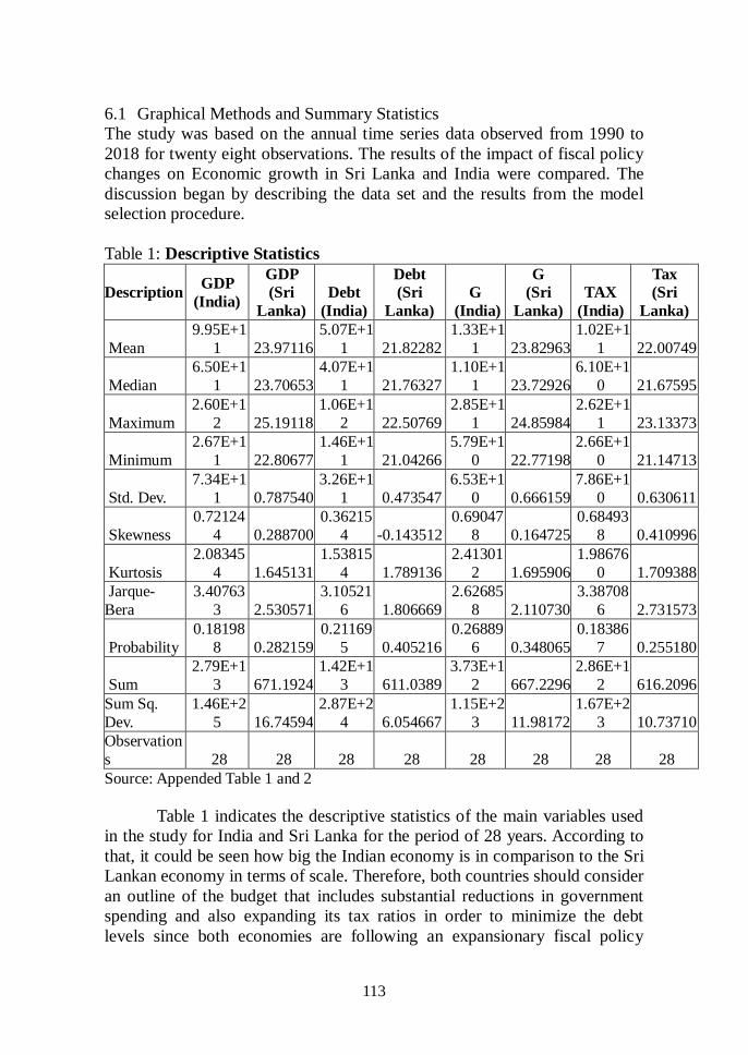
6.1 Graphical Methods and Summary Statistics
The study was based on the annual time series data observed from 1990 to
2018 for twenty eight observations. The results of the impact of fiscal policy
changes on Economic growth in Sri Lanka and India were compared. The
discussion began by describing the data set and the results from the model
selection procedure.
Table 1: Descriptive Statistics
Description GDP
(India)
GDP
(Sri
Lanka)
Debt
(India)
Debt
(Sri
Lanka)
G
(India)
G
(Sri
Lanka)
TAX
(India)
Tax
(Sri
Lanka)
Mean
9.95E+1
1 23.97116
5.07E+1
1 21.82282
1.33E+1
1 23.82963
1.02E+1
1 22.00749
Median
6.50E+1
1 23.70653
4.07E+1
1 21.76327
1.10E+1
1 23.72926
6.10E+1
0 21.67595
Maximum
2.60E+1
2 25.19118
1.06E+1
2 22.50769
2.85E+1
1 24.85984
2.62E+1
1 23.13373
Minimum
2.67E+1
1 22.80677
1.46E+1
1 21.04266
5.79E+1
0 22.77198
2.66E+1
0 21.14713
Std. Dev.
7.34E+1
1 0.787540
3.26E+1
1 0.473547
6.53E+1
0 0.666159
7.86E+1
0 0.630611
Skewness
0.72124
4 0.288700
0.36215
4 -0.143512
0.69047
8 0.164725
0.68493
8 0.410996
Kurtosis
2.08345
4 1.645131
1.53815
4 1.789136
2.41301
2 1.695906
1.98676
0 1.709388
Jarque-
Bera
3.40763
3 2.530571
3.10521
6 1.806669
2.62685
8 2.110730
3.38708
6 2.731573
Probability
0.18198
8 0.282159
0.21169
5 0.405216
0.26889
6 0.348065
0.18386
7 0.255180
Sum
2.79E+1
3 671.1924
1.42E+1
3 611.0389
3.73E+1
2 667.2296
2.86E+1
2 616.2096
Sum Sq.
Dev.
1.46E+2
5 16.74594
2.87E+2
4 6.054667
1.15E+2
3 11.98172
1.67E+2
3 10.73710
Observation
s 28 28 28 28 28 28 28 28
Source: Appended Table 1 and 2
Table 1 indicates the descriptive statistics of the main variables used
in the study for India and Sri Lanka for the period of 28 years. According to
that, it could be seen how big the Indian economy is in comparison to the Sri
Lankan economy in terms of scale. Therefore, both countries should consider
an outline of the budget that includes substantial reductions in government
spending and also expanding its tax ratios in order to minimize the debt
levels since both economies are following an expansionary fiscal policy
114
regime. The government should grow GDP and reduce deficits that are run
every year and try to balance the debt portfolio. In order to simplify these
relationships to identify the composite relationship we have used the other
significant econometric tools as discussed below.
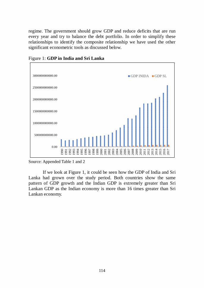
Figure 1: GDP in India and Sri Lanka
0.00
500000000000.00
1000000000000.00
1500000000000.00
2000000000000.00
2500000000000.00
3000000000000.00
199
0
199
1
199
2
199
3
199
4
199
5
199
6
199
7
199
8
199
9
200
0
200
1
200
2
200
3
200
4
200
5
200
6
200
7
200
8
200
9
201
0
201
1
201
2
201
3
201
4
201
5
201
6
201
7
GDP INIDA GDP SL
Source: Appended Table 1 and 2
If we look at Figure 1, it could be seen how the GDP of India and Sri
Lanka had grown over the study period. Both countries show the same
pattern of GDP growth and the Indian GDP is extremely greater than Sri
Lankan GDP as the Indian economy is more than 16 times greater than Sri
Lankan economy.

115
Figure 2: Taxation, Expenditure, and Debt (a) Sri Lanka (b) India
Source: Appended Table 1 and 2
-70000000000.00
-60000000000.00
-50000000000.00
-40000000000.00
-30000000000.00
-20000000000.00
-10000000000.00
0.00
10000000000.00
20000000000.00
1985 1990 1995 2000 2005 2010 2015 2020
EXP TAX Debt
a. Sri Lanka
b. India

116
According to Figure 2, both countries recorded the same pattern of
expansionary expenditure policy with higher debt levels. Since this budget
deficit is widening continuously, the debt level is worsening as a chronic
epidemic during the period.
6.2 Unit Root Test Results
In order to model the variable in a manner that captures the inherent
characteristics of its time series, this study used the Akaike Information
Criterion (AIC) to determine the lag structure of the series.
Once the maximum length of the lag is selected, Augmented Dickey-
Fuller test was performed on each variable at level form and the results are
shown in Table 2.
Table 2: Unit Root Test Results
Variable
First difference
Data (Sri Lanka)
First Difference Data (India)
ADF Test Statistic
Intercept and Trend Intercept and Trend
Gross Domestic
Product
-3.565 (0.031) [-3.622] -5.411 (0.000) [-3.595]
Debt -3.927 (0.025) [-3.622] -6.589 (0.000) [-3.592]
Tax Revenue -4.285 (0.011) [-3.595] -5.285 (0.000) [-3.233]
Source: Appended Table 1 and 2
ADF unit root test with Mackinnon one-side p-values done for level
data established the fact that all the level data in the variables used in this
modal were non-stationary at 5% significant level and in with intercept and
trend included in the equation. Therefore, developing a model based on non-
stationary data series is not desirable. Hence, to make the research modal
validated, the stationary could be tested in the first difference level and by
performing a Engal – Granger co-integrating test it could be made sure that
this research modal is valid as a result of the variables become stationary in
first difference and the said variables co-integrated in long run making a long
run relationship between the variables. The table shows the ADF results
when the test was performed on 1st difference on each variable. ADF Unit
root test of 1st difference data has been used to reject the null hypothesis and
accept the alternative hypothesis. This made sure that all the variables
concerned were stationary at difference level and their level of integration is
I(1). If the variables were not stationary at level form, but stationary at first
difference, then a valid long run relationship modal could be developed on
level data provided that the series were co-integrated in the long run.
117
Engle and Granger (1987) established that “if each element of a
vector of time series Xt is stationary only after differencing, but a linear
combination Xt needs not be differenced, the time series Xt have been
defined to be co-integrated of order with co-integration vector .
Interpreting Xt = 0 as a long run equilibrium, co-integration implies that
equilibrium holds except for a stationary, finite variance disturbance even
though the series themselves are non-stationary and have finite variance.” To
test the co-integration, the Engle- Granger test on residual of the model
should be run using level data. The long run relationship of the study for Sri
Lanka is:
lnGDPsl= β0 + lnTexp+ β2 lnTexp+ β3 lnTdebt + Ut
Applied model is
lnGDPsl= β0 + lnTexp+ β2 lnTexp+ β3 lnTdebt
U = error term.
The long run relationship of the study for India is:
lnGDPI= β0 + lnTexp+ β2 lnTexp+ β3 lnTdebt + Ut
Applied model is:
lnGDPI= β0 + lnTexp+ β2 lnTexp+ β3 lnTdebt
GDP= Gross domestic production in India
Texp= Government Expenditure
Tdebt = Total debt
U is the residual of the modal and it is called as error correction term and to
test the co-integrating property of the residual using Engle- Granger test was
conducted. In Engle- Granger test hypothesis was:
H0: Residual series has a unit root
H1: Residual series does not have a unit root.
The R2 is 0.9962 and the Durbin-Watson statistic is 1.2638. Since R2<DW
Statistic, the series is not spurious and suitable for regression. Also,
calculating residual of this regression estimate was stationary at level form,
the model was suitable for regression and to obtain log run relationship
(Engle and Granger, 1987).
Since p-value for ADF was less than 0.05 (0.0329), it also supported
to decide that the null hypothesis of the residual series had a unit root that
can be rejected and accept the alternative hypothesis that the residual series
had no unit root. The variables used in the model was non-stationary at
level, but stationary at first difference. Then the residual series of the model
was stationary at level. Therefore, the model co-integrated and could be
considered as long run model.
118
The R2 is 0.9960 and the Durbin-Watson statistic was 1.0920. Since
R2<DW Statistic, the series was not spurious and suitable for regression.
Also, calculating residual of this regression estimate was stationary at level
form, the model was suitable for regression and to obtain log run relationship
(Engle and Granger, 1987). Since p value for ADF was less than 0.05
(0.0329), it also supported to decide that the null hypothesis of the residual
series had a unit root could be rejected and accept the alternative hypothesis
that the residual series had no unit root. The variables used in the model was
non-stationary at level, but stationary at first difference. Then the residual
series of the model was stationary at level. Therefore, the model co-
integrated and could be considered as long run model.
6.3 Long Run Relationship
Engel Grager Cointegration between the levels variables, estimated through
the OLS method for Sri Lanka as follows:
lnGDP= β0 + lnTexp+ β2 lnTexp+ β3 lnTdebt
lnGDPSL= -4.075993+ 0.01lnTexp+0.51lnTtax-0.68lnTdebt (3)
According to equation 3, estimated results confirms that in the long
run following relationships exist:
a) 100% increase in Total Government Spending will improve the GDP
only by 1% in the long run in Sri Lanka during the study period.
b) 100% increase in Total tax revenue will improve the GDP by 51% in
the long run in Sri Lanka during the study period.
c) 100% increase in Total debt will reduce the GDP by 68% in the long
run in Sri Lanka during the study period.
Engel Grager Cointegration between the levels variables, estimated through
the OLS method for India as follows:
lnGDP= β0 + lnTexp+ β2 lnTexp+ β3 lnTdebt
lnGDPIND= -2.713388+ 0.59lnTexp+0.57lnTtax-0.01lnTdebt (4)
According to equation 4, estimated results confirmed that in the long
run following relationships exist:
a) 100% increase in Total Government Spending will improve the GDP
by 59% in the long run in India during the study period.
b) 100% increase in Total tax revenue will improve the GDP by 57% in
the long run in India during the study period.
c) The impact of debt on economic growth in India is not significant as
the probability value is (0.8301).
119
Therefore, according to the results, the main conclusion is that India’s
expenditure policy directly enhances countries economic growth (59%)
while Sri Lanka’s expenditure policy enhances growth only by less than 1%.
Therefore, Sri Lanka also follows the investment oriented expenditure policy
by increasing capital expenditure and reducing high scale of recurrent
expenditure.
6.4 Short Run Relationship
In order to test for causality between the series GDP and fiscal policy tools
through the ECM, it is necessary to verify if the two series are cointegrated.
The following function represents Sri Lanka’s short run relationship:
∆lnGDP= β0 + ∆lnTexp+ ∆β2 lnTtax+ ∆β3 lnTdebt
∆lnGDPSL= 0.009626 + 0.01lnTexp+0.32lnTtax-0.73lnTdebt (5)
As shown in equation 5, estimated results confirms that in the short
run following relationships are existing:
a) 100% increase in Total Government Spending will improve the GDP
by 1% in the short run which is not significant in Sri Lanka.
b) 100% increase in Total tax revenue will increase the GDP by 32% in
the short run during the study period in Sri Lanka.
c) 100% increase in Total debt will reduce the GDP by73% in the short
run during the study period in Sri Lanka.
∆lnGDPIND = 0.004204+ 0.6 lnTexp+0.59lnTta+-0.01lnTdebt (6)
As shown in equation 6, estimated results confirmed that in the short
run following relationships are existing:
a) 100% increase in Total Government Spending will improve the
GDP by 60% in the short run in India.
b) 100% increase in Total tax revenue will increase the GDP by 59%
in the short run during the study period in India.
c) 100% increase in Total debt will improve the GDP by 1% in the
short run during the study period in India.
According to the estimated results for the short run relationship,
India’s fiscal policy is very effective in enhancing economic growth while
Sri Lanka’s fiscal policy does not make any significant impact in the short
run except the taxation. Therefore, Sri Lanka should get her way out of
prevailing ad hoc fiscal policies.
120
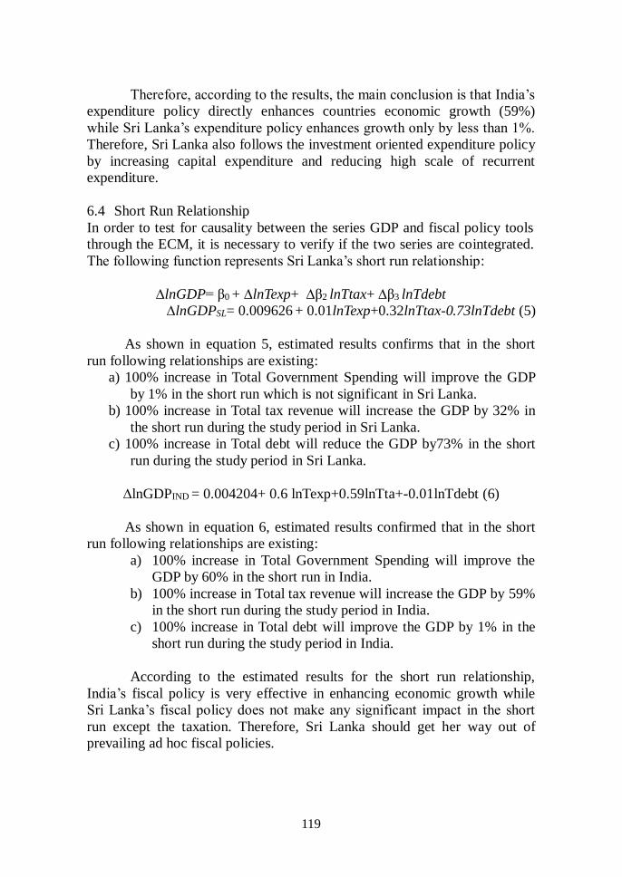
6.5 Causal Relationship
The above analysis suggests that there exists a long-run relationship between
government revenue and expenditure in both countries. But, in the direction
of determining which variable causes the other, Granger causality test was
used. The Granger causality test results are presented in Table 3 for Sri
Lanka.
Table 3: Granger Causality Test Results for Sri Lanka Null Hypothesis: Obs F-Statistic Prob.
LNGGFCE does not Granger Cause LNGDP 26 0.48059 0.6251
LNGDP does not Granger Cause LNGGFCE 1.73462 0.2008 LNTAX does not Granger Cause LNGDP 26 0.05286 0.9486
LNGDP does not Granger Cause LNTAX 1.01868 0.3782 LNDEBT does not Granger Cause LNGGFCE 26 2.92881 0.0755
LNGGFCE does not Granger Cause LNDEBT 1.05839 0.3648 Source: Appended Table 1 and 2
According to Table 3, the estimated results for bi-directional causality
for the fiscal policy instruments on economic growth in Sri Lanka recorded a
significant relationship for all the variables.
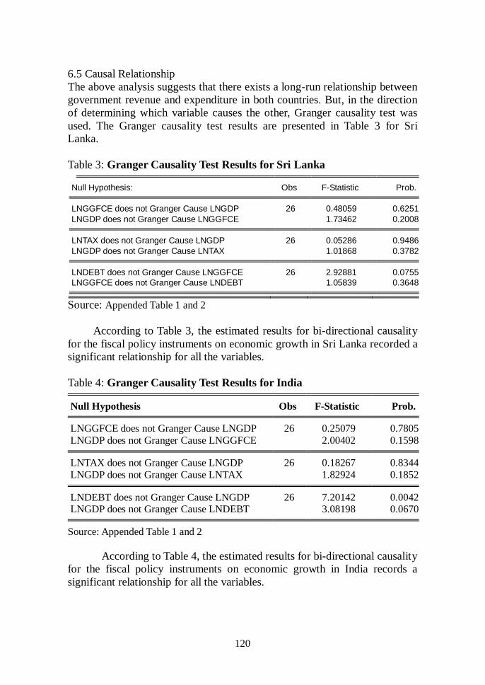
Table 4: Granger Causality Test Results for India
Null Hypothesis Obs F-Statistic Prob. LNGGFCE does not Granger Cause LNGDP 26 0.25079 0.7805
LNGDP does not Granger Cause LNGGFCE 2.00402 0.1598 LNTAX does not Granger Cause LNGDP 26 0.18267 0.8344
LNGDP does not Granger Cause LNTAX 1.82924 0.1852
LNDEBT does not Granger Cause LNGDP 26 7.20142 0.0042
LNGDP does not Granger Cause LNDEBT 3.08198 0.0670
Source: Appended Table 1 and 2
According to Table 4, the estimated results for bi-directional causality
for the fiscal policy instruments on economic growth in India records a
significant relationship for all the variables.

121
6.5 Impact of External Shocks (Impulse Response Function Results)
Figure 3: Response of GDP due to the Shocks to the Government
Spending in Sri Lanka
Source: Appended Table 1 and 2
When there is a shock to the government spending, that will not
generate any significant effect on the GDP during the first five years and
then the shock will improve the GDP gradually in Sri Lanka.
Figure 4: Response of GDP due to the Shocks to the Government
Spending in India
Source: Appended Table 1 and 2
When there is a shock to the Government Spending in India, that will
positively affect the GDP and the GDP will improve sharply during the first
three years because of the external shock. Then the impact will decay slowly.

122
According to the results obtained from the Impulse Response Function, it
can be concluded that, the Indian economy is comparatively strong enough to
handle external shocks with compared to Sri Lankan economy.
7. Conclusion
Overall, the theoretical framework discussed in this study was premised on
the endogenous growth theory which analyses the nature of the relationship
between fiscal policy variables and economic growth in the economies of Sri
Lanka and India. With this, the relationship between output in the economies
and the other variables to be used for this study are specified were tested.
Estimated results confirm that in the long run following relationships exist;
100% increase in Total Government Spending will improve the GDP by 1%
in Sri Lanka while Indian economy improves by 59%. Total tax revenue will
increase the GDP by 51% while India’s 57%. In the short run, there is no
significant impact of fiscal policy variables on economic growth in Sri Lanka
but Indian economy grows with the expansionary fiscal policy in the short
run. According to the Impulse Response Function results, when an external
shock affects the total government spending level, Sri Lankan economy does
not adequately respond but Indian economy is strong enough to handle the
external shocks which affect the country’s spending level.
8. Policy Recommendations
There is overwhelming evidence that government spending is not effective in
Sri Lanka compared to Indian economy and that Sri Lanka’s economy could
grow much faster if the burden of government was reduced. Taxes on goods
and services and deficits are both harmful, but the real problem is that
government is taking money from the private sector and spending it in ways
that are often counterproductive in Sri Lankan context. Fiscal policy should
focus on reducing the level of government spending on nonproductive
purposes as Indian economy does, with particular emphasis on those
programs that yield the lowest benefits or impose the highest costs.
Therefore, shrinking the size of recurrent expenditures and enhancing capital
expenditure should be a major goal for policymakers in Sri Lanka. If this is
considered, the Sri Lankan economy certainly would perform better, and this
would boost prosperity and make Sri Lanka more competitive. India also
should continue this towards the “East Asian Model” of economic growth.
References
Amirthalingam, K. (2013). Importance and Issues in Taxation in Sri Lanka.
Colombo Business Journal, Vol. 4, No. 1, Colombo.
Andrei, B. (2015). The Fiscal Consolidation Consequences on Economic
Grwoth in Romania. Journal of Economic Forecasting.
123
Central Bank of Sri Lanka, Annual Reports, Various Years.
Dilrukshini, W. A. (2009). Public Expenditure and Economic Growth in Sri
Lanka. Staff Studies, 32(1), 32. doi:10.2156/ss.v47i1.3210.
Hanusch, H., Chakraborty, L. S., and Khurana, S. (2017). Fiscal Policy,
Economic Growth and Innovation: An Empirical Analysis of G20
Countries. Levy Economics Institute of Brad College. Working paper
no. 883
Yadav, S., Upadhyaya, V., and Sharma, S. (2010). Impact of Fiscal Policy
Shocks on the Indian Economy. The Journal of Applied Economic
Research (SAGE).213 -248
Sylvia, A. (2015). Fiscal Policy and Economic Growth in Nigeria. Sage
Open. 113-124

124
Appendices
Table 1: Variables in India
INDIA
GDP GGFCE TAX DEBT
1990 316697337894.51 57986433014.44 32899428571.43 167181142857.14
1991 266502281094.12 57889097922.40 29647007042.25 145773327464.79
1992 284363884080.10 59887311516.47 32850792253.52 166447623239.44
1993 275570363431.90 63441938514.13 26570007107.32 161127221037.67
1994 322909902308.89 64319850480.66 29402357438.67 162349792927.68
1995 355475984177.45 69339244204.33 34258392362.18 176332306744.69
1996 387656017798.60 72556990656.15 36250563063.06 179548423423.42
1997 410320300470.28 80721445535.65 38289053905.39 214052255225.52
1998 415730874171.13 90563350637.71 34790466973.14 215776917493.35
1999 452699998386.91 101228493960.20 39831168831.17 236788265306.12
2000 462146799337.70 102621260010.58 41894888888.89 261561777777.78
2001 478965491060.77 105036246931.59 39605970781.28 289309337285.62
2002 508068952065.90 104841668586.11 44480872069.11 320690867955.57
2003 599592902016.35 107751924990.15 54580686695.28 372677253218.88
2004 699688852930.28 112035851169.62 67349381625.44 440463780918.73
2005 808901077222.84 121987100238.73 83197455123.84 513552601681.44
2006 920316529729.75 126592187775.17 104782473998.67 561761009072.80
2007 1201111768410.27 138708510596.13 143967718446.60 683643203883.50
2008 1186952757636.11 153100199205.08 139437456807.19 727753973738.77
2009 1323940295874.06 174350535549.63 129248137417.22 728031870860.93
2010 1656617073124.71 184413340746.95 173728806133.63 862819277108.43
2011 1823049927772.05 197063742482.04 160521754829.39 813170247337.06
2012 1827637859136.23 198261940845.90 188558180227.47 881790026246.72
2013 1856722121394.42 199393834825.95 196419262555.63 898250158931.98
2014 2039127446299.30 214519083464.87 234608008075.37 1010001682368.78
2015 2102390808997.09 229001374041.58 217944003593.35 950247042970.51
2016 2274229710530.03 256841425530.38 241148454827.74 997475972201.69
2017 2597491162897.67 284936364638.75 262279334770.56 1063222513089.01
125
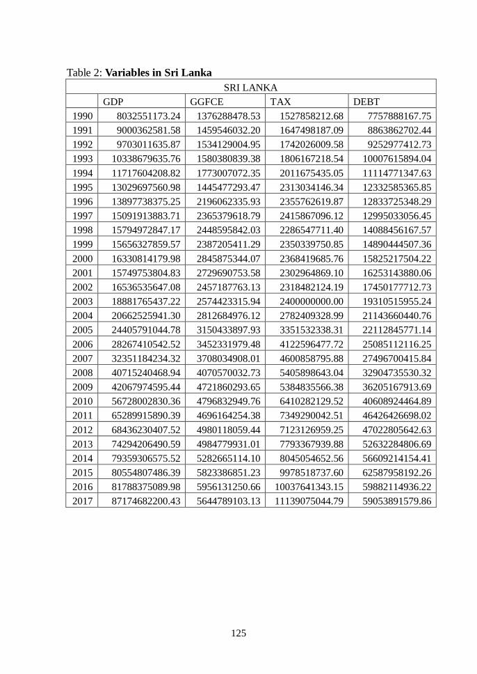
Table 2: Variables in Sri Lanka
SRI LANKA
GDP GGFCE TAX DEBT
1990 8032551173.24 1376288478.53 1527858212.68 7757888167.75
1991 9000362581.58 1459546032.20 1647498187.09 8863862702.44
1992 9703011635.87 1534129004.95 1742026009.58 9252977412.73
1993 10338679635.76 1580380839.38 1806167218.54 10007615894.04
1994 11717604208.82 1773007072.35 2011675435.05 11114771347.63
1995 13029697560.98 1445477293.47 2313034146.34 12332585365.85
1996 13897738375.25 2196062335.93 2355762619.87 12833725348.29
1997 15091913883.71 2365379618.79 2415867096.12 12995033056.45
1998 15794972847.17 2448595842.03 2286547711.40 14088456167.57
1999 15656327859.57 2387205411.29 2350339750.85 14890444507.36
2000 16330814179.98 2845875344.07 2368419685.76 15825217504.22
2001 15749753804.83 2729690753.58 2302964869.10 16253143880.06
2002 16536535647.08 2457187763.13 2318482124.19 17450177712.73
2003 18881765437.22 2574423315.94 2400000000.00 19310515955.24
2004 20662525941.30 2812684976.12 2782409328.99 21143660440.76
2005 24405791044.78 3150433897.93 3351532338.31 22112845771.14
2006 28267410542.52 3452331979.48 4122596477.72 25085112116.25
2007 32351184234.32 3708034908.01 4600858795.88 27496700415.84
2008 40715240468.94 4070570032.73 5405898643.04 32904735530.32
2009 42067974595.44 4721860293.65 5384835566.38 36205167913.69
2010 56728002830.36 4796832949.76 6410282129.52 40608924464.89
2011 65289915890.39 4696164254.38 7349290042.51 46426426698.02
2012 68436230407.52 4980118059.44 7123126959.25 47022805642.63
2013 74294206490.59 4984779931.01 7793367939.88 52632284806.69
2014 79359306575.52 5282665114.10 8045054652.56 56609214154.41
2015 80554807486.39 5823386851.23 9978518737.60 62587958192.26
2016 81788375089.98 5956131250.66 10037641343.15 59882114936.22
2017 87174682200.43 5644789103.13 11139075044.79 59053891579.86