flash calcination of limestone in a bench-scale sorbent

FLASH CALCINATION OF LIMESTONE IN A BENCH-SCALE SORBENT ACTIVATION

PROCESS (SAP) UNIT

BY

IVAN SUGIYONO

THESIS

Submitted in partial fulfillment of the requirements

for the degree of Master of Science in Environmental Engineering in Civil Engineering

in the Graduate College of the

University of Illinois at Urbana-Champaign, 2012

Urbana, Illinois

Adviser:

Dr. Massoud Rostam-Abadi

Professor Mark J. Rood

ii

ABSTRACT

Coal-fired power plants produce 40 % of the total electricity in the United States. The

flue gas generated from burning coal contains air pollutants including sulfur oxides (SOx),

hydrochloric acid (HCl) and elemental and ionic mercury (Hgo and Hg2+). A process option to

remove these pollutants from the flue gas is by injection of sorbents downstream of a boiler and

up-stream of a particulate control device. Activated carbon (AC) is a suitable sorbent to capture

vapor-phase mercury and calcium-based sorbents such as quicklime (CaO) and hydrated lime

(Ca(OH)2) are suitable sorbents to capture SOx and HCl. This research addresses producing

quicklime by a novel process to remove SOx and HCl from flue gas streams. Quicklime is

commercially prepared by thermal decomposition of limestone (CaCO3) in a rotary kiln. The

surface area of commercial quicklime, a key parameter of reactivity, is typically < 2 m2/g.

Therefore, increasing the surface area of quicklime in a cost-effective process would enhance its

effectiveness as a sorbent for control of combustion-generated air pollutants.

Illinois State Geological Survey (ISGS), a division of the Prairie Research Institute at the

University of Illinois at Urbana Champaign (UIUC), and Electric Power Research Institute

(EPRI), Palo Alto, CA, have developed a patent-pending Sorbent Activation Process (SAP)

technology for on-site production and direct injection of quicklime into flue gas generated by

coal fired power plants (US Patent Application 20,110,223,088). This process is an extension of

a similar patented process for on-site production of activated carbon (AC) to remove vapor-phase

mercury emissions in the flue gas (US Patents 6, 451, 094 and 6,558,454). SAP utilizes an

entrained-flow reactor in which sorbent (AC or quicklime) particles are subjected to a < 5 second

residence time during their production. On-site production of quicklime could help lower the

production cost of quicklime sorbent for dry sorbent injection (DSI) applications.

In this research, a bench-scale SAP unit (2 kg/hr limestone feed rate) was used to prepare

quicklime from two limestone samples. The impacts of particle size, surface morphologies of

limestone, and operating parameters of SAP including temperature profile, and residence time on

the product quicklime were investigated. SAP experiments were designed to provide engineering

data and guidelines for operating a pilot-scale (20 kg/hr limestone feed rate) and designing a full-

scale SAP units (135 kg/hr limestone feed rate) currently being tested at a coal-fired power plant

in the United States. Additionally, kinetic information about calcination of the two limestone

iii

samples was obtained from the analysis of non-isothermal decomposition measured by

thermogravimetric analysis (TGA) method. Furthermore, the kinetic information was used to

predict limestone calcination in SAP.

Lime sorbents prepared in SAP contained between 20 and 80 wt % calcium oxide

(balance calcium carbonate) and had surface areas ranging between 5 and 12 m2/g depending on

operation conditions employed. Non-isothermal TGA experiments were analyzed by several data

analysis approaches including Coats-Redfern, Criado linearization and DTG-curve fitting

method using DTG-SIM software to obtain the kinetic parameters (activation energy, frequency

factor, and reaction order) for thermal decomposition (calcination) of the two limestone samples.

The values of the kinetic parameters were in good agreement with those previously reported in

the literature. The kinetic models predicted the experimental TGA calcination in N2 with less

than 10% deviation. However, only the Coats-Redfern-based kinetic model predicted the TGA

calcinations in CO2 data with less than 10 % deviation. The kinetic parameters were used to

predict limestone conversions in an ideal flash calciner and in SAP. Ideal flash calciner assumed

isothermal condition throughout the reactor while the later one used the actual temperature

profiles in SAP to predict limestone conversion at different CO2 partial pressures. The impact of

mass and heat transfer limitation, lime sintering phenomenon, and particle size distribution of

limestone/lime were not included in the model. The experimental limestone conversions were

higher than those predicted by the models.

Based on the results from SAP experiments and model predictions, it was concluded that

the actual temperature of limestone particle was likely much higher than the gas temperature

measured in SAP. Future work should include: 1) installation of additional thermocouples to

continuously monitor both axial and radial temperature profiles in the SAP, 2) an understanding

of the flow pattern and hydrodynamic inside the SAP to better estimate gas-gas and gas-solid

mixing, 3) testing several size-graded limestone samples to evaluate the impact of particle size

on limestone calcination, 4) calibrating the propane and combustion air flow rates to obtain more

accurate readings, 5) quantify the extent of particle deposition in SAP, 6) measure gas phase

concentrations of CO, CO2, O2, NOx, and hydrocarbons (HCs), and verify those measured

values, and 7) incorporate mass and heat transports effects in the model to better predict

calcination performance of limestone in bench-, pilot-, and full-scale SAPs.

iv

To my parents, brother and friends whose support and prayers are simply never-ending.

v

ACKNOWLEDGEMENTS

I thank my advisors Dr. Massoud Rostam-Abadi and Dr. Mark J. Rood for providing

guidance and support throughout my graduate study. All of the technical discussion and casual

interaction with them have honed my technical and social skills. Their life-time advices will

always be invaluable for my future endeavors.

I am truly privileged to be part of two amazing research groups, Advanced Energy

Technology Initiative (AETI) and Air Quality Engineering and Sciences (AQES). Special thanks

are reserved for Dr. Yonqi Lu, Dr. Seyed A. Dastgheib, Dr. Hong Lu, and David Ruhter whose

opinions, recommendations, and helps have always been significant for my research. I am also

grateful to all AQES research group members for providing friendship and insight. Their

presence in the past two years has made my journey very enjoyable. Last but not least, I would

like to thank my God, parents, brother, and friends for their never-ending encouragement,

support, and faith on me which always keep me motivated and confident.

Characterization work, including SEM and some of the TGA, was performed at the

Frederick Seitz Material Research Laboratory Central Facilities, University of Illinois, which are

partially supported by the U.S. Department of Energy under grants DE-FG02-07ER46453 and

DE-FG02-07ER46471.

This work is supported by grants from Electric Power Research Institute (EPRI C6220,

C5150), University of Illinois at Urbana Champaign (D7355, D7155), and Illinois Clean Coal

Institute (ICCI-A2322).

vi

TABLE OF CONTENTS

LIST OF TABLES ....................................................................................................................... viii

LIST OF FIGURES ........................................................................................................................ x

1 INTRODUCTION ................................................................................................................... 1

1.1 Background ...................................................................................................................... 1

1.2 Limestone Decomposition ................................................................................................ 2

1.2.1 General Limestone Calcination ................................................................................. 2

1.2.2 Mass and Heat Transport Processes in Limestone Decomposition .......................... 2

1.2.3 Difficulties in Postulating a Unified Limestone Calcination Model ........................ 5

1.3 Lime Production Methods ................................................................................................ 7

1.3.1 Slow Heating Calcination ......................................................................................... 7

1.3.2 Flash Calcination ...................................................................................................... 8

1.4 Environmental Applications of Calcium-Based Sorbents ................................................ 8

1.4.1 Gaseous Pollutants Removal ..................................................................................... 8

1.4.2 Impact of SO3 on Mercury Removal in Activated Carbon Injection (ACI) Processes 12

1.5 Benefits of SAP Sorbents to Pollutants Control Technique Utilizing DSI .................... 16

1.6 Objectives and Contributions of This Research ............................................................. 17

2 MATERIAL AND METHODS............................................................................................. 18

2.1 Experimental .................................................................................................................. 18

2.1.1 Sample Preparation ................................................................................................. 18

2.1.2 Material Characterizations ...................................................................................... 19

2.1.3 Calcination in Bench-Scale SAP ............................................................................ 23

2.2 Kinetics of Thermal Decomposition of Limestone ........................................................ 33

vii

2.2.1 Non-Isothermal TGA Calcination ........................................................................... 33

2.2.2 Determination of Kinetic Parameters ...................................................................... 38

2.2.3 Quantification of Deviation between Predicted and Experimental Data ................ 41

3 RESULTS AND DISCUSSIONS ......................................................................................... 42

3.1 Bench-Scale SAP Experiment ........................................................................................ 42

3.2 Characterization of Limestone and Lime Products ........................................................ 55

3.2.1 Particle Size ............................................................................................................ 55

3.2.2 Surface Morphologies ............................................................................................. 58

3.3 Calcination Kinetics ....................................................................................................... 60

3.3.1 Temperature Profile in a 80 µm Limestone Particle in SAP .................................. 60

3.3.2 TGA Calcination in N2............................................................................................ 62

3.3.3 TGA Calcination in CO2 ......................................................................................... 81

3.4 Predicting Extent of Calcination in a Flash Calciner ..................................................... 98

3.5 Predicting Extent of Calcination in SAP ...................................................................... 107

4 SUMMARY, CONCLUSIONS AND FUTURE WORK ................................................... 119

Appendix A ................................................................................................................................. 122

REFERENCES ........................................................................................................................... 126

viii

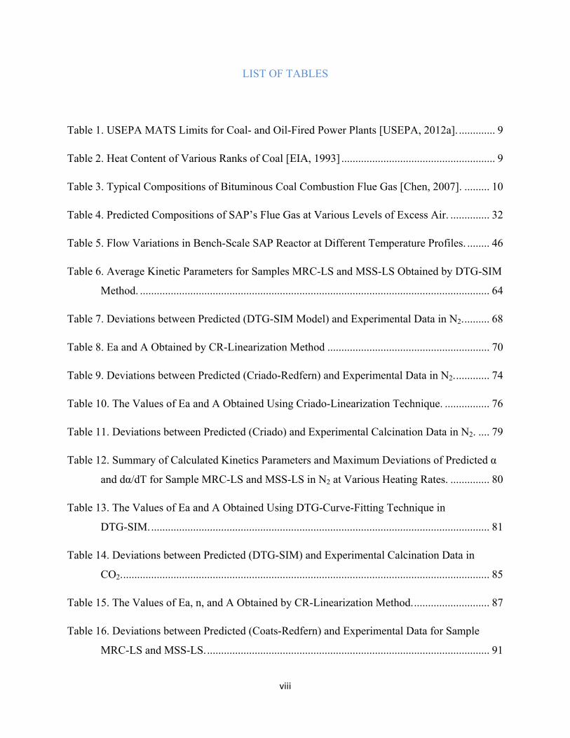
LIST OF TABLES

Table 1. USEPA MATS Limits for Coal- and Oil-Fired Power Plants [USEPA, 2012a]. ............. 9

Table 2. Heat Content of Various Ranks of Coal [EIA, 1993] ....................................................... 9

Table 3. Typical Compositions of Bituminous Coal Combustion Flue Gas [Chen, 2007]. ......... 10

Table 4. Predicted Compositions of SAP’s Flue Gas at Various Levels of Excess Air. .............. 32

Table 5. Flow Variations in Bench-Scale SAP Reactor at Different Temperature Profiles. ........ 46

Table 6. Average Kinetic Parameters for Samples MRC-LS and MSS-LS Obtained by DTG-SIM

Method. ............................................................................................................................. 64

Table 7. Deviations between Predicted (DTG-SIM Model) and Experimental Data in N2. ......... 68

Table 8. Ea and A Obtained by CR-Linearization Method .......................................................... 70

Table 9. Deviations between Predicted (Criado-Redfern) and Experimental Data in N2. ............ 74

Table 10. The Values of Ea and A Obtained Using Criado-Linearization Technique. ................ 76

Table 11. Deviations between Predicted (Criado) and Experimental Calcination Data in N2. .... 79

Table 12. Summary of Calculated Kinetics Parameters and Maximum Deviations of Predicted α

and dα/dT for Sample MRC-LS and MSS-LS in N2 at Various Heating Rates. .............. 80

Table 13. The Values of Ea and A Obtained Using DTG-Curve-Fitting Technique in

DTG-SIM. ......................................................................................................................... 81

Table 14. Deviations between Predicted (DTG-SIM) and Experimental Calcination Data in

CO2. ................................................................................................................................... 85

Table 15. The Values of Ea, n, and A Obtained by CR-Linearization Method. ........................... 87

Table 16. Deviations between Predicted (Coats-Redfern) and Experimental Data for Sample

MRC-LS and MSS-LS. ..................................................................................................... 91

ix

Table 17. The Values of Ea and A Obtained by Criado-Linearization Method ........................... 93

Table 18. Deviations between the Predicted (Criado) and Experimental Data in CO2. ............... 97


and dα/dT for Sample MRC-LS and MSS-LS in CO2 at Various Heating Rates. ............ 97

x

LIST OF FIGURES

Figure 1. Temperature and Partial Pressure of CO2 Profiles during the Five Sub-Processed of

Limestone Calcination [Cheng, 2006]. ............................................................................... 4

Figure 2. Equilibrium Curve of Limestone Decomposition [Baker, 1962]. ................................... 4

Figure 3. SEM Images of Lime at Various Sintering Levels [Oates, 1998]. .................................. 7

Figure 4. Neck-Growth Mechanism between Two Lime Grains [German and Munir, 1976]. ...... 7

Figure 5. Schematic Diagram of ACI Process in Coal-Fired Power Plants. ................................. 13

Figure 6. Impact of Surface Area of SAP-Derived AC on Hg-Removal Efficiencies Normalized

to the Commercial PAC (Darco-Hg) [Rostam-Abadi, et al., 2009]. ................................. 14

Figure 7. SAP-Enhanced ACI Schematic Diagram. ..................................................................... 14

Figure 8. Impact of SO3 on Mercury Removal Efficiency by ACI [Feeley, et al., 2009]. ........... 15

Figure 9. Schematic Diagram of On-Site Co-Production of AC and Lime by SAP at Power

Plant. ................................................................................................................................. 15

Figure 10. Limestone Utilization in DSI without SAP. ................................................................ 16

Figure 11. Limestone Utilization in DSI with SAP. ..................................................................... 16

Figure 12. Research Flow Diagram. ............................................................................................. 18

Figure 13. HORIBA's LA-300 Laser Diffraction Particle Size Distribution Analyzer. ............... 20

Figure 14. Monosorb B.E.T. Surface Area Analyzer. .................................................................. 21

Figure 15. Hitachi S-4700 SEM.................................................................................................... 21

Figure 16. Emitech 575 Sputter Coater. ........................................................................................ 22

Figure 17. Schematic Diagram of Thermo Scientific Versatherm TGA (Thermo Scientific,

2011). ................................................................................................................................ 22

xi

Figure 18. Front View of the Bench-Scale SAP Reactor. ............................................................. 24

Figure 19. Propane and Air Supply Lines into the Bench-Scale SAP Reactor. ............................ 24

Figure 20. Sample Collection Unit at the Exit of the Bench-Scale SAP. ..................................... 25

Figure 21: AccuRate Dry Material Feeder 300. ............................................................................ 26

Figure 22: Limestone Feed Line Set-Up Designs. A) Initial Design. B) Modified Design. ........ 26

Figure 23. Calibration Curve of Limestone Feed Rate. ................................................................ 27

Figure 24. Calibration Curve of Feeder’s Nitrogen Flow Rate. ................................................... 27

Figure 25. Calibration Curve of Propane Flow Rate. ................................................................... 28

Figure 26. Calibration Curve of Combustion Air Flow Rate. ...................................................... 28

Figure 27. Schematic of Design of Cyclone. ................................................................................ 29

Figure 28. Ferret 16 GasLink II Emission Analyzer. .................................................................... 30

Figure 29. Three Different Segments of SAP. .............................................................................. 33

Figure 30. Impacts of Kinetic Parameters on TG (Equation 26) and DTG (Equation 27)

Models............................................................................................................................... 40

Figure 31. DTG-SIM’s Algorithm to Determine the Best Kinetic Parameters [Yang, et al.,

2001]. ................................................................................................................................ 40

Figure 32. Combustion Efficiency, CO and HCs Concentrations in the Flue Gas at Different O2

Concentrations in the Flue Gas [Biarnes, 2012]. .............................................................. 43

Figure 33. Equilibrium Composition and Temperature of Adiabatic Combustion of kerosene

CH1.8 at Different Equivalent Ratios [Flagan and Seinfeld, 1988]. .................................. 43

Figure 34. Comparisons between Predicted Equilibrium Concentrations and Measured

Concentrations of CO and HCs at Different ϕs. ............................................................... 44

xii

Figure 35. Comparisons between Predicted Equilibrium Concentrations of CO and Measured

Concentrations of CO and HCs at Different ϕs. ............................................................... 45

Figure 36. Comparisons of Terminal Settling Velocity of a Limestone Particle with 60 µm

Particle Size and Gas Velocity at Different Temperatures. .............................................. 48

Figure 37. Extent of Particle Settling at Different Temperature Profiles in SAP. ........................ 48

Figure 38. Temperature Profiles in Bench-Scale SAP at Various Operating Conditions. ........... 49

Figure 39. EC of Lime Sorbents Produced from MSS-LS (Blue) and MRC-LS (Orange) at

Different T1. ...................................................................................................................... 50

Figure 40. Predicted Adiabatic Propane Flame Temperature at Different ϕs. .............................. 51

Figure 41. Total Surface Area of Lime Produced from MSS-LS (Blue) and MRC-LS (Orange).53

Figure 42. Carbonate-Free Surface Area of Carbonate-Free Limes Produced from MSS-LS (Blue

Symbols) and MRC-LS (Orange Symbols). ..................................................................... 54

Figure 43. (a) Extent of Calcination and (b) Surface Area of lime produced from Z7

Limestone. ......................................................................................................................... 55

Figure 44. Particle Size Distribution of Sample MSS-LS before Injection to SAP. .................... 56

Figure 45. Particle Size Distribution of Sample MRC-LS before Injection to SAP. .................... 56

Figure 46. Particle Size Distribution of Sample MRC-LS Calcined in the SAP at 825 K. .......... 57

Figure 47. Particle Size Distribution of Sample MRC-LS Calcined in the SAP at 950 K. .......... 57

Figure 48. Particle Size Distribution of Sample MRC-LS Calcined in the SAP at 1,050 K. ....... 57

Figure 49. Particle Size Distribution of Sample MRC-LS Calcined in the SAP at 1,120 K. ....... 58

Figure 50. SEM Images of a) Raw MSS-LS and b) Raw MRC-LS. ............................................ 59

Figure 51. SEM Images of Lime Product from Calcination of a) Sample MSS-LS and b) Sample

MRC-LS at 1,180 K in the SAP. ...................................................................................... 59

xiii

Figure 52. SEM Images of Limes Produced from Calcination of Sample MRC-LS a) SAP at

1,550 K, b) Batch Reactor at 1,273 K in N2. .................................................................... 59

Figure 53. Heisler Chart for Determining the Center Temperature of a Sphere with Radius of

ro. ....................................................................................................................................... 61

Figure 54. Heat up rate of a 80 µm Limestone Particle at Different Gas Temperatures in an

Entrained-Flow Reactor. ................................................................................................... 61

Figure 55. TG and DTG Data from Calcination of Sample MRC-LS in N2. ............................... 63

Figure 56. TG and DTG Data from Calcination of Sample MSS-LS in N2. ................................ 64

Figure 57. Comparison of Predicted (DTG-SIM) and Experimental α and dα/dT of Sample

MRC-LS at 10 K/min in N2. ............................................................................................. 65


MRC-LS at 5 K/min in N2. ............................................................................................... 66


MRC-LS at 2 K/min in N2. ............................................................................................... 66

Figure 60. Comparison of Predicted (DTG-SIM) and Experimental α and dα/dT of Sample MSS-

LS at 10 K/min in N2. ....................................................................................................... 67


LS at 5 K/min in N2. ......................................................................................................... 67


LS at 2 K/min in N2. ......................................................................................................... 68

Figure 63. CR-Linearized Plot (Equation 31) for MRC-LS Calcination at 2, 5, and 10 K/min in

N2. ..................................................................................................................................... 69

Figure 64. CR-Linearized Plot (Equation 31) for MSS-LS Calcination at 2, 5, and 10 K/min in

N2. ..................................................................................................................................... 70

xiv

Figure 65. Comparison of Predicted (CR-Based) and Experimental α and dα/dT of Sample MRC-

LS at 10 K/min in N2. ....................................................................................................... 71


LS at 5 K/min in N2. ......................................................................................................... 71


LS at 2 K/min in N2. ......................................................................................................... 72

Figure 68. Comparison of Predicted (CR-Based) and Experimental α and dα/dT of Sample MSS-

LS at 10 K/min in N2. ....................................................................................................... 72


LS at 5 K/min in N2. ......................................................................................................... 73


LS at 2 K/min in N2. ......................................................................................................... 73

Figure 71. Criado-Linearized Plot (Equation 37) for Sample MRC-LS Calcined at 2, 5, and 10

K/min in N2. ...................................................................................................................... 75

Figure 72. Criado-Linearized Plot (Equation 37) for Sample MSS-LS Calcined at 2, 5, and 10

K/min in N2. ...................................................................................................................... 75

Figure 73. Comparison of Predicted (Criado) and Experimental α and dα/dT of Sample MRC-LS

Calcined at 10 K/min in N2. .............................................................................................. 76


Calcined at 5 K/min in N2. ................................................................................................ 77



Figure 76. Comparison of Predicted (Criado) and Experimental α and dα/dT of Sample MSS-LS

Calcined at 10 K/min in N2. .............................................................................................. 78



xv




MRC-LS at 5 K/min in 10 kPa PCO2. ................................................................................ 82






LS at 5 K/min in 10 kPa PCO2. .......................................................................................... 83





Figure 85. CR-Linearized Plot (Equation 31) for MRC-LS Calcination at 5 K/min and Various

CO2 Concentrations. .......................................................................................................... 86



Figure 87. Comparison of Predicted (CR) and Experimental α and dα/dT of Sample MRC-LS at

5 K/min in 10 kPa CO2. .................................................................................................... 88


5 K/min in 25 kPa CO2. .................................................................................................... 89


5 K/min in 50 kPa CO2. .................................................................................................... 89

xvi

Figure 90. Comparison of Predicted (CR) and Experimental α and dα/dT of Sample MSS-LS at 5

K/min in 10 kPa CO2. ....................................................................................................... 90


K/min in 25 kPa CO2. ....................................................................................................... 90


K/min in 50 kPa CO2. ....................................................................................................... 91

Figure 93. Criado-Linearized Plot (Equation 37) for MRC-LS Calcination at 5 K/min and

Various CO2 Concentrations. ............................................................................................ 92

Figure 94. Criado-Linearized Plot (Equation 37) for MSS-LS Calcination at 5 K/min and Various



at 5 K/min in 10 kPa CO2. ................................................................................................ 94


at 5 K/min in 25 kPa CO2. ................................................................................................ 94


at 5 K/min in 50 kPa CO2. ................................................................................................ 95


at 5 K/min in 10 kPa CO2. ................................................................................................ 95


at 5 K/min in 25 kPa CO2. ................................................................................................ 96

Figure 100. Comparison of Predicted (Criado) and Experimental α and dα/dT of Sample MSS-

LS at 5 K/min in 50 kPa CO2. ........................................................................................... 96

Figure 101. EC of Sample MRC-LS at 825 K. ........................................................................... 100

Figure 102. EC of Sample MRC-LS at 950 K. ........................................................................... 100

Figure 103. EC of Sample MRC-LS at 1,050 K. ........................................................................ 101

xvii





Figure 108. EC of Sample MSS-LS at 825 K. ............................................................................ 103

Figure 109. EC of Sample MSS-LS at 950 K. ............................................................................ 104

Figure 110. EC of Sample MSS-LS at 1,050 K. ......................................................................... 104





Figure 115. Temperature Profile across SAP at Different Residence Times. ............................ 109

Figure 116. EC Prediction for Sample MRC-LS by NONISO T Model at T1 = 825 K. ............ 109

Figure 117. EC Prediction for Sample MRC-LS by NONISO T Model at T1 = 950 K. ............ 110

Figure 118. EC Prediction for Sample MRC-LS by NONISO T Model at T1 = 1,050 K. ......... 110





Figure 123. EC Prediction for Sample MSS-LS by NONISO T Model at T1 = 825 K. ............. 113

Figure 124. EC Prediction for Sample MSS-LS by NONISO T Model at T1 = 950 K. ............. 113

xviii

Figure 125. EC Prediction for Sample MSS-LS by NONISO T Model at T1 = 1,050 K. .......... 114





Figure 130. Comparisons of Experimental and Modeled EC in SAP for Sample MRC-LS. ..... 117

Figure 131. Comparisons of Experimental and Modeled EC in SAP for Sample MSS-LS. ...... 118

1

1 INTRODUCTION

1.1 Background

Limestone (calcium carbonate, CaCO3) is an abundant natural resource and a low-cost

material (US$ 10 – 20/ metric ton) for producing limes [Smith, 2001]. When heated, limestone

will decompose and release its CO2 content and this process is known as limestone calcination.

The product of limestone calcination is mainly quicklime (CaO). However, depending on the

relative humidity (RH) and temperature of the calcination gas the produced CaO can react with

H2O and form hydrated lime (Ca(OH)2),. Both quicklime and hydrated lime are effective

sorbents for capturing gaseous pollutants, such as sulfur oxides (SOx including SO2 and SO3) and

hydrochloric acid (HCl), in coal combustion flue gases [Morris, 2011]. SOx are the precursors for

acid rain, which can acidify lakes and streams, accelerate the decay of building materials and

paints, and jeopardize public health [Likens, 2010]. HCl is acidic and corrosive. Surface area of

quicklime and hydrated lime impacts its reactivity with sulfur oxides and hydrochloric acid gases

[Borgwardt, 1985]. This study focused on producing high-surface-area quicklime as a product of

limestone calcination using a novel process concept.

Commercial quicklime is conventionally produced in a rotary kiln where limestone

particles (1 – 5 cm particle size) are heated for several hours at above 1,173 K [British Lime

Association, 2011]. Otherwise noted, the size of any particle in this thesis always refers to the

widest straight edge-to-edge distance in a particle. Exposing quicklime to high temperature in the

kiln for a long residence time results in surface area < 2 m2/g due to sintering of reactive sites

[Oates, 1998]. Increasing the surface area and porosity and decreasing the particle size of lime

increases its chemical reactivity with SO2 [Borgwardt and Harvey, 1972] and HCl [Yan, et al.,

2003]. An alternative method, flash calcination process, uses an entrained-flow reactor

(residence time in seconds) to decompose pulverized limestone particles (< 100 µm particle size)

limes that have higher surface area (up to 60 m2/g) and porosity (void fraction of 0.5) than those

prepared in conventional kilns [Silcox, et al., 1989].

Researchers at the Illinois State Geological Survey (ISGS), a division of Prairie Research

Institute at the University of Illinois at Urbana Champaign (UIUC), and Electric Power Research

Institute (EPRI) have developed a Sorbent Activation Process (SAP) for on-site production of

2

activated carbon (AC) for mercury emission control from coal combustion flue gases (US

Patents 6,451,094 and 6,558,454). A full-scale demonstration of this technology was recently

completed at a utility site in Illinois. SAP technology consists of a proprietary entrained-flow

reactor. SAP has also been proposed for on-site production of quicklime (US Patent

20,110,223,088) to capture SOx and HCl in coal combustion flue gases. Successful development

of on-site sorbent production with SAP could potentially reduce the cost of gaseous pollutant

emissions controls at coal power plants. In this study, a bench-scale SAP unit, designed and

fabricated in 1995 and now located at the Applied Research Laboratory (ARL) of ISGS, was

used to evaluate the impacts of operating conditions of SAP on physical and chemical properties

of quicklime produced from two limestone samples. The bench-scale SAP unit has a capacity of

2 kg/hr limestone feed rate. Furthermore, non-isothermal thermogravimetric analysis (TGA)

experiments were performed to determine the kinetics of calcination of limestone samples in N2

and CO2. TGA-derived reaction rates were employed to develop models to predict extent of

calcination (EC) or conversion (α) of limestone in SAP.

1.2 Limestone Decomposition

1.2.1 General Limestone Calcination

Calcium carbonate, or limestone, thermally decomposes, or calcines, to calcium oxide by

releasing carbon dioxide (Equation 1). The calcination reaction is reversible and endothermic

(4.6 MJ heat required/kg of quicklime produced) [Oates, 1996]. Some limestone may contain

minor amounts of calcium hydroxide which also decomposes to quicklime during the calcination

reaction (Equation 2). In this study, limestone decomposition, or calcination, always refers to the

decomposition of calcium carbonate to quicklime (Equation 1).

Equation 1 CaCO3 (s) ↔ CaO (s) + CO2 (g) ; Keq = PCO2

Equation 2 Ca(OH)2 (s) ↔ CaO (s) + H2O (g) ; Keq = PH2O

1.2.2 Mass and Heat Transport Processes in Limestone Decomposition

Limestone decomposition is a gas-solid reaction in which the solid is the reactant. The

reaction involves mass- and heat-transfer processes between a solid limestone particle and the

3

calcination gas. The sequence of steps to convert limestone to quicklime includes five sub-

processes as shown in Figure 1:

1. Transport of heat from the bulk gas at temperature TA by radiation and convection to the

solid surface (at radius, rs) at temperature Ts (symbolized by α).

2. Transport of heat by conduction into the limestone particle to the reaction front (at radius

of rF) at temperature TF through a porous layer of lime (symbolized by λ).

3. Dissociation reaction of CaCO3 to CaO and CO2 at the reaction interface (symbolized

with k). The difference between the equilibrium partial pressure of CO2, P*

CO2, (Figure

2), and the partial pressure of CO2 at the reaction interface, PF, is the driving force of

limestone calcination reaction (Equation 1). The enthalpy of the calcination reaction is

considered much larger than the internal energy; hence, the heat transport into limestone

particle is negligible and the core temperature, TM, is only slightly lower than TS [Cheng,

2006]. PF is higher than the partial pressure of CO2 at the gas-solid interface, PS, and in

the bulk gas, PA, because CO2 is generated in-situ during the calcination reaction.

4. Transport of generated CO2 at the reaction interface through the porous lime layer to the

outer surface of the particle (symbolized with Dp,eff) to maintain the continuity of

calcination reaction at the reaction interface.

5. Transport of CO2 by a convection transport from the outer surface of the particle to the

bulk gas with a partial pressure of CO2 of PA (symbolized by β) [Cheng, 2006].

4

Figure 1. Temperature and Partial Pressure of CO2 Profiles during the Five Sub-Processed of

Limestone Calcination [Cheng, 2006].

Figure 2. Equilibrium Curve of Limestone Decomposition [Baker, 1962].

A shrinking core reaction model has been widely employed to describe thermal

decomposition of a limestone particle [Ingraham and Marier, 1963; Beruto and Searcy, 1974;

Elder and Reddy, 1986; Zhong and Bjerle, 1993; Fonseca, et al., 1998; Eversen, et al., 2006].

This reaction model describes conversion of a nonporous limestone solid particle in which the

0

20

40

60

80

100

120

800 850 900 950 1000 1050 1100 1150 1200

PC

O2

(kP

a)

Temperature (K)

5

reaction occurs at the outer surface and progresses into the interior of the limestone. With the

progress of the calcination reaction, a layer of porous lime product is developed around the

unreacted core of limestone.

1.2.3 Difficulties in Postulating a Unified Limestone Calcination Model

Modeling limestone calcination is a complex process. This complication is caused by

uncertainties in identifying the rate limiting steps amongst the aforementioned five sub-

processes, unique micro-structures and crystallography in different types of limestone, and

changes in structures of the surface layers of lime by sintering [Oates, 1998].

1.2.3.1 Rate Limiting Step of Limestone Calcination

Satterfield and Feakes (1959) reported three different rate controlling steps of limestone

calcination which included steps 1, 3, and 4 described in section 1.2.2. Hyatt, et al. obtained

calcination data using a TGA method and developed a calcination model based on chemical

kinetics limitation (step 3) [Hyatt, et al., 1958]. Beruto and Searcy observed a constant rate of

reaction until 80% of a 1 mm outer slice of a limestone particle had decomposed [Beruto and

Searcy, 1974]. Beyond this conversion, the rate decreased because a 30-µm-thick metastable

CaO layer separating the unreacted CaCO3 and the stable-oriented CaO layer was formed. Ohme

et al. reported that below 1,273 K, limestone decomposition in an entrained-flow reactor was

kinetically limited. Borgwardt used an entrained-flow reactor and reported that for particle

diameter < 90 µm, limestone decomposition was kinetically controlled except during the final

stages of decomposition where the diffusion of CO2 through the product layer also became rate

limiting [Borgwardt, 1985]. Khinast, et al. utilized a one-dimensional mathematical particle

model that included mass transfer and diffusion in lime and limestone pore structures, diffusion

through the lime product layer, heat transfer and heat conduction in the particle, reaction at the

CaO/CaCO3 interface and evolution of the pore structure in the particle during the calcination

reaction [Khinast, et al., 1995]. They reported that heat transfer and product layer diffusion are of

minor importance compared to the chemical reaction and particle diffusion resistance. On the

other hand, both Hills and Campbell, et al. reported that heat transfer and product layer diffusion

were the rate limiting steps [Hills, 1968; Campbell, et al., 1970]. Ingraham and Marier as well as

Thompson found that only mass transfer through the product layer was the rate-limiting step

6

[Ingraham and Marier, 1963; Thompson, 1979]. As a conclusion, there is not a general

agreement about the mechanism of limestone calcination in part because porosity, grain size,

particle size, and chemical composition of limestone and calcination process conditions impact

the mechanism. [Borgwardt, 1989a and b; Oates, 1998].

1.2.3.2 Sintering Phenomena in Limestone Calcination

Sintering of lime occurs because freshly generated grains grow in size and coalesce upon

exposure to temperatures > 1,000 K. A direct impact of sintering is lowering the surface area and

thus chemical reactivity of lime. Scanning Electron Microscopy (SEM) images of lime at

different sintering levels (Figure 3) reveal higher sintering levels in denser quicklime [Oates,

1998]. The mechanism of sintering involves transfer of lime grains during neck growth and grain

fusion [Borgwardt, 1989a]. Figure 4 illustrates the neck-growth in sintering phenomena between

two lime grains [German and Munir, 1976]. Keener and Kuang (1992) reported that sintering

rate of lime was accelerated with increasing calcination temperature. Rapid surface area and

logarithmic porosity decreases were consequences of sintering during the calcination reaction

[Borgwardt, 1989a]. Borgwardt prepared a 104 m2/g calcium oxide by calcining a 25 mg of high-

purity limestone in 6 L/min N2 flow using a differential reactor at 973 K for < 90 seconds

[Borgwardt, 1989a]. He concluded that: 1) increasing particle size of limestone decreased the

rate of sintering; however, the rate of sintering was independent of particle diameter between 2 –

20 µm, and 2) CO2 and water vapors in calcination gas tended to promote sintering [Borgwardt,

1989b]. Boynton reported that the presence of high levels of sodium in limestone reduced

sintering of quicklime while finely dispersed silica, alumina and iron oxide increased sintering

[Boynton, 1980].

7

Figure 3. SEM Images of Lime at Various Sintering Levels [Oates, 1998].

Figure 4. Neck-Growth Mechanism between Two Lime Grains [German and Munir, 1976].

1.3 Lime Production Methods

Nowadays quicklime can be produced by either slow heating in a rotary kiln or fast

heating in an entrained-flow reactor known as flash calcination [Oates, 1998].

1.3.1 Slow Heating Calcination

In commercial practice, the calcination process uses a direct-fired rotary kiln that uses

coal or natural gas as its fuel. The particle size of the feed limestone is ≤ 10 cm and has a specific

surface area of ≤ 1 m2/g. The calcination temperature is generally above 1,173 K and the

calcination time ranges between 2 and 4 hours. Quicklime produced commercially under such

conditions have a low surface area (< 2 m2/g) [Oates, 1998].

8

The time-temperature history during calcination reactions greatly impacts the conversion

of the raw limestone to quicklime and the surface area of the formed quicklime. Partial pressure

of CO2 in the calcination gas determines the decomposition temperature of limestone and the rate

at which the calcination reaction proceeds. The high calcination temperature and the long

residence time in the kiln are the main reasons for the low surface area of the lime products.

These factors contribute to grain growth by sintering, whereby the individual lime grains in a

particle adhere to each other resulting in grain growth and a lower surface area per mass of

particle [Oates, 1998].

1.3.2 Flash Calcination

In a flash calcination process, pulverized limestone particles (< 100 μm) are rapidly

calcined in an entrained-flow reactor operating at temperature between 823 and 1,023 K and < 3

second residence time [Dinsdale, et al., 2011]. Grain growth by sintering and, therefore, surface

area deactivation are much less pronounced when pulverized limestone is calcined under rapid

heating and short residence time process conditions. For example, the specific surface area of

CaO formed by calcination of limestone or dolomite with particle size between 10 and 90 μm

particles at 1,123 to 1,348 K and < 1-second residence time ranged between 50 and 63 m2/g

[Borgwardt, 1985]. Flash calcined limes had little internal porosity, smaller grain size and plate-

like grain shape [Zhong and Bjerle, 1993], while limes produced by slow heating and flash

calcination processes displayed non-uniform grains which were jointed together by necks to form

a continuous porous matrix [Milne, et al., 1990].

1.4 Environmental Applications of Calcium-Based Sorbents

1.4.1 Gaseous Pollutants Removal

Utility industry is among the top emitters of gaseous pollutants such as Hg, SOx, and HCl

to the atmosphere. On December 16, 2011, the United States Environmental Protection Agency

(USEPA) announced the latest Mercury and Air Toxins Standards (MATS), Table 1, for new and

existing coal- and oil-fired electric utility steam generating units (EGUs) [USEPA, 2012a]. The

MATS rule will be implemented by 2014. Some coal-fired power plants utilize wet limestone

scrubbing for SOx control. The removal efficiency of SOx by wet absorption technique range

between 90 and 98% [Schenelle and Brown, 2002]; however, this technique is relatively

9

expensive (US$200 – 500/metric ton pollutant for a power plant with > 400-MW capacity and

US$500 – 5,000/metric ton pollutant for a power plant with < 400-MW) and not suitable for

smaller and older coal power plants [USEPA, 2012b]. Dry Sorbent Injection (DSI) processes are

considered as an alternative option for some power plants to remove SOx and HCl in the flue gas

due to their lower capital and overall emissions control costs than a wet scrubbing system [EPA-

452/F-03-034, 2012b]. In DSI processes, a sorbent such as lime, or hydrated lime, or Trona, or

sodium bicarbonate is injected into the flue gas upstream of a particulate control device (PCD).

Targeted gaseous pollutants are adsorbed onto the sorbent through chemical bonds. The spent

sorbent is collected in the PCD and disposed of along with coal ash in an environmentally

acceptable manner.

Table 1. USEPA MATS Limits for Coal- and Oil-Fired Power Plants [USEPA, 2012a].

Component Generation Rate (g/MWh)

Hg 0.006 – 0.05

SO2 680

HCl 9

1.4.1.1 Coal-Fired Power Plants

40% of the total electricity production in the U.S. is supplied by coal-fired power plants

[USEPA, 2012a]. Coal combustion is an exothermic reaction and the amount of heat generated

from it varies depending on the rank of coal burned (Table 2) [EIA, 1993]. Coal combustion

produces CO2 and water (main reaction products), various pollutants such as nitrogen oxides

(NOx), SO2, SO3, HCl (in ppmv concentrations) and various trace metal species such as mercury

and selenium, in ionic and elemental forms (in ppbv concentrations). Table 3 shows the typical

composition of a bituminous coal combustion flue gas.

Table 2. Heat Content of Various Ranks of Coal [EIA, 1993]

Rank of Coal Heat Content (MJ/kg)

Bituminous 21 – 27

Sub-bituminous 16 – 21

Lignite < 16

10

Table 3. Typical Compositions of Bituminous Coal Combustion Flue Gas [Chen, 2007].

Component Amount

N2 (mol %) 76 – 77

O2 (mol %) 4.4

H2O (mol %) 6.2

CO2 (mol %) 12.5 – 12.8

SO2 (ppmv) 1500

CO (ppmv) 50

NOx (ppmv) 420

HCl (ppmv) 3

Hg (µg/m3) 5 – 10

1.4.1.2 Control of Gaseous Pollutants by Quicklime

Chemical reactions of quicklime with SOx and HCl are as described below.

Equation 3 CaO (s) + SO2 (g) + 0.5 O2 (g) → CaSO4 (s)

Equation 4 CaO (s) + SO3 (g) → CaSO4 (s)

Equation 5 CaO (s) + 2 HCl (g) ↔ CaCl2 (s) + H2O (g)

1.4.1.2.1 Sulfur Oxides Reactions with Calcium-Based Sorbent

Studies of sulfur oxides reaction with calcium-based sorbents were conducted extensively

in 1970s and 1980s. Borgwardt used a differential reactor to measure the rate of SO2 reaction

(Equation 3) with calcium oxide particles < 500 µm in diameter [Borgwardt, 1970]. He found

that the reaction rate is first order with respect to SO2 concentration. Borgwardt and Harvey

showed that the reaction is chemically controlled up to 1,253 K, and < 50% calcium conversion

(conversion of CaO to CaSO4) was obtained when pores in the < 100 µm CaO particles were >

0.1 µm. At conversions > 50%, the pores became completely filled with CaSO4 and the rate-

limiting mechanism shifted from chemical reaction to solid diffusion [Borgwardt and Harvey,

1972]. The concentration of oxygen also affected the structure of the product layer, CaSO4

[Allen and Hayhurst, 1996; Dennis and Hayhurst, 1990]. They claimed that increasing

11

concentration of oxygen when the temperature was > 923 K produced a large number of cracks

in the sorbent which helped the diffusion of CO2 through the product layer; thus increasing

conversion of CaO to CaSO4.

At temperatures below 800 K, carbonation and hydration of CaO impact the rate of

sulfation reaction. Hartman and Trnka (1993), Klingspor, et al. (1983), and Liu and Shih (2008)

investigated the reactions of different Ca-based sorbents with SO2 at temperatures below 775 K.

Relative humidity of the reaction gas was determined to be a key parameter for SO2 reaction with

CaO. At least 20 % RH was required to obtain > 50 % SO2 removal [Klingspor et al., 1983].

Increasing RH from 20 to 70 % improved SO2 removal by 4 times at 340 K [Khinast, 1995 and

Irabien, et al., 1992]. Carbonation reaction in a 10 – 40 % by volume CO2 gas did not interfere

with the sulfation of CaO when the concentration of SO2 was > 2,000 ppmv [Rochelle, et al.,

1990]. This conclusion was also confirmed by Harman and Trnka [Harman and Trnka, 1993].

The presence of NOx, O2 and CO2 in the flue gas doubled the rate of sulfation of calcium oxide

to CaSO4 at 330 K [Liu and Shih, 2008].

Kocaefe, et al. investigated the sulfation rate of a reagent-grade CaO with SO2 and SO3

using a TGA and showed that below 600 K, CaO only reacted with SO3 [Kocaefe, et al., 1985].

Benson et al. confirmed this conclusion by showing that SO2 did not react at an appreciable rate

with Ca(OH)2 between 422 and 450 K; however, SO3 reacted efficiently with Ca(OH)2 [Benson,

et al., 1998. The reaction rate of CaO with SO3 was faster than SO2 at all temperatures at

comparable concentrations of SO2 and SO3 [Kocaefe, et al., 1985]. It was shown that the initial

reaction rate was first order with respect to SO3 concentration. Thibault, et al. studied the kinetics

of SO3 reaction with calcium oxide samples in a fixed bed reactor and concluded that for < 170

µm CaO particles, the reaction rate was independent of particle size because the diffusional

resistance associated with individual grains was dominant [Thibault, et al., 1982].

1.4.1.2.2 HCl Reaction with Calcium-Based Sorbents

Reactions of HCl with calcium-based sorbents are similar to those of the sulfur oxides

described in section 1.4.1.2.1. The rate of reaction of CaO with HCl is first order with respect to

the concentration of HCl under a reaction controlled region [Yan, et al., 1993]. The HCl reaction

with CaO was more favorable than SO2 at 923 K [Daoudi and Walters, 1991]. Above this

12

temperature, the HCl reaction rate remained unchanged. Similar to SO2 and SO3 reactions with

basic oxides, HCl reaction with CaO was kinetically controlled at conversions < 10 % and > 10

%, it was controlled by reaction kinetics and product layer diffusion [Fonseca, et al., 2003]. To

achieve conversions > 98 %, the presence of moisture was required and in the absence of

moisture, only 5 % conversion was achieved [Fonseca, et al., 1998].

1.4.2 Impact of SO3 on Mercury Removal in Activated Carbon Injection (ACI) Processes

1.4.2.1 Mercury Regulation

Mercury is a bio-accumulative toxin which can cause deformities on fetus, impair

nervous system and lead to lethality at high concentrations [USEPA, 2012c]. Coal-fired power

plants are the largest source of mercury emission in the U.S. (45 metric ton/year), generating 45

% of the U.S. total emissions [USEPA, 2012a]. To date, 19 states, including Illinois, require

mercury reduction standards for coal- and oil-fired power plants. In December 2011, USEPA

finalized MATS rule which limit the toxic pollutants from coal-power plant including mercury.

When implemented, coal fired power plants are required to practice the MACT standards and

meet 0.006-0.05 g/MWh mercury emission by 2014 [USEPA, 2012a].

1.4.2.2 Mercury Removal from Combustion Gases with Activated Carbon Injection

Activated carbon injection (ACI) process is emerging as an affective low cost technology

for removal of vapor-phase mercury from coal combustion flue gases [Hoffmann and Ratafia-

Brown, 2003 and Zhuang, 2011]. In ACI, powdered activated carbon (PAC) is injected into the

flue gas ductwork of a coal-fired power plant, downstream of boiler and up-stream of PCD such

as a baghouse or an electrostatic precipitator (ESP). PAC adsorbs the vapor-phase mercury in

the flue gas and is collected with the fly ash in the PCD. Depending on the type of coal burned

and PCD installed on the plant, ACI can reduce mercury emissions by > 90 % [Hoffmann and

Ratafia-Brown, 2003]. The schematic diagram of the ACI process in coal-fired power plants is

shown in Figure 5.

13

Figure 5. Schematic Diagram of ACI Process in Coal-Fired Power Plants.

1.4.2.3 Sorbent Activation Process (SAP)

SAP is a technology for on-site production of PAC at power plants using the same coal

burned for electricity generation. This technology was developed by ISGS and EPRI and is

currently being demonstrated at full-scale (US Patents 6, 451, 094 and 6,558,454). PAC

produced in bench, pilot, and full-scale SAP units from different types of coal had comparable

mercury-removal performances to the commercial Darco-Hg activated carbon (manufactured by

Norit Americas) as shown in Figure 6 [Rostam-Abadi, et al., 2009].

In SAP, pulverized coal is injected into an entrained-flow reactor in which coal

devolatilization and coal char activation reactions occur in < 3 seconds. The heat of reactions in

SAP is provided by burning the volatile matters released during the initial devolatilization stage

of the coal, or by burning an auxiliary fuel (propane). PAC produced in SAP is directly injected

in to the flue gas duct upstream of an existing ESP or a baghouse. Figure 7 shows the schematic

diagram of the implementation of SAP technology in an ACI process in coal-fired power plants.

EPRI has estimated that SAP technology would reduce the cost of ACI for mercury control by at

least 50 % [EPRI, 2010].

14

Figure 6. Impact of Surface Area of SAP-Derived AC on Hg-Removal Efficiencies Normalized

to the Commercial PAC (Darco-Hg) [Rostam-Abadi, et al., 2009].

Figure 7. SAP-Enhanced ACI Schematic Diagram.

1.4.2.4 Impact of SO3 on Hg Removal by AC

Mechanisms of mercury adsorption onto AC are very complex. Contributing parameters

include pore-size distribution, carbon surface chemistry, flue gas constituents (HCl, SOx, NOx),

temperature, and concentrations of mercury species (elemental or oxidized) in the flue gas

[Zhuang, 2011; Hsi, et al., 2001]. Results from pilot-scale and full-scale ACI tests have shown

total mercury removal up to 95 % for low-sulfur flue gas [Lee, 2003, 2004]. However, the

presence of SO3 in the flue gas, even at concentration as low as 10 part per million (ppmv),

0

100

200

300

400

0% 20% 40% 60% 80% 100%

Relative Hg adsorption capacity, [(g Hg/g sorb.) / (g Hg/g FGD-AC )]

BE

T, m

2/g-

Sam

ple

PRB lignite Illinois

Relative Hg Adsorption Capacity, [(g Hg/g sample) / (g Hg/g Darco-Hg)]

15

significantly reduce the ACI’s Hg removal because SO3 and Hg compete to bind onto AC sites,

Figure 8 [Feeley, et al., 2009].

Figure 8. Impact of SO3 on Mercury Removal Efficiency by ACI [Feeley, et al., 2009].

To enhance mercury removal in a high-sulfur flue gas, either a carbon that inhibits SO3

adsorption should be used or SO3 in the flue gas should to be removed. Injection of quicklime or

hydrated lime into flue gas is one option to remove SO3. SAP is being considered for co-

production of AC and quicklime for control of mercury emissions from high-sulfur flue gas (US

Patent 20,110,223,088). Figure 9 shows the implementation of SAP technology in a DSI process

for on-site co-production of AC and quicklime at coal-fired power plants.

Figure 9. Schematic Diagram of On-Site Co-Production of AC and Lime by SAP at Power Plant.

0

20

40

60

80

100

0 50 100 150

Mer

cury

Rem

oval

(%

)

ACI Concentration (mg/m3)

Labadie (DARCOHg-LH/Hot-side/NoSO3)Labadie (DARCOHg-LH/Hot-side/10.3ppm SO3)Labadie (DARCOHg-LH/No SO3)

Labadie (DARCOHg-LH/10.3 ppmSO3)

Darco Hg-LH/Hot-Side/No SO3

Darco Hg-LH/Hot-Side/10.3 ppmv SO3

Darco Hg-LH/No SO3

Darco Hg-LH/10.3 ppmv SO3

16

1.5 Benefits of SAP Sorbents to Pollutants Control Technique Utilizing DSI

Lime production in SAP is a flash calcination process because pulverized limestone

particles (< 100 µm) are exposed to a hot flue gas in a few seconds (< 5 seconds). Figure 10 and

Figure 11 show the step-by-step processes of limestone utilization in DSI application without

and with SAP. On-site production of lime via SAP clearly simplifies the DSI process at a utility

site. It shortens the production time of the sorbent and also increases the availability of the

sorbent at the plant. Storing a reactive sorbent and maintaining its reactivity can be costly. Thus,

DSI-SAP technique can reduce the storage cost by stocking limestone instead of lime sorbent. A

large amount of limestone fine (particle size < 45 µm) is often produced during grinding and

sieving operations at limestone and lime companies. It is commonly disposed of in quarries

because commercial demand for limestone fine is not large; hence it can be purchased at a lower

cost than size-graded limestone and used as a feedstock in SAP, further reducing the cost of

producing quicklime. Lime sorbent produced in SAP has a high surface area (between 5 to 12

m2/g) and fresh active sites to enhance its reactivity. Hence, DSI-SAP represents an innovative

approach to reduce emission control costs in coal-fired power plants.

Figure 10. Limestone Utilization in DSI without SAP.

Figure 11. Limestone Utilization in DSI with SAP.

17

1.6 Objectives and Contributions of This Research

The main objective of this research is to study the feasibility of producing quicklime for

DSI application using a bench-scale SAP and to determine the impacts of SAP’s operating

conditions such as temperature profile, residence time, and gaseous composition on the

percentage of CaCO3 decomposed to CaO and surface area of product quicklime. The second

objective is to investigate the kinetics of limestone calcination using non-isothermal TGA

technique and to develop models to predict thermal decomposition of limestone in SAP.

Achieving these engineering objectives is very important to help provide design data for scale up

of SAP and predict limestone calcination behavior in pilot-scale and full-scale SAP studies.

18

2 MATERIAL AND METHODS

2.1 Experimental

Experimental work performed in this research included limestone calcination tests to

determine the impact of operating conditions of bench-scale SAP on the physical and chemical

properties of lime products, characterization of limestone samples and product limes produced in

the SAP, non-isothermal TGA calcination experiments to determine kinetic parameters of

thermal decomposition of limestone samples, and developing reaction models to predict

limestone calcination in SAP. Research flow diagram of this study is described in Figure 12.

Figure 12. Research Flow Diagram.

2.1.1 Sample Preparation

Two limestone samples were tested. Sample MSS-LS was obtained from Mississippi

Lime Company and sample MRC-LS was obtained from Mercury Research Center (MRC) at

19

Gulf Utility in Pensacola, Florida. The latter sample was used in several pilot-scale SAP tests at

MRC. Two 10 kg buckets of each pulverized limestone were shipped to ISGS. As-received

pulverized limestone samples were dried overnight at 333 K at atmospheric pressure. Each 10 kg

limestone bucket was riffled into four 2.5 kg to obtain uniform and representative samples for

characterization and calcination experiments. These 2.5 kg portions of limestone were stored in

closed plastic buckets at ambient air temperature and pressure.

2.1.2 Material Characterizations

Material characterizations included analysis of particle size distribution, surface area,

surface morphology, and CaO content or EC or conversion of a sample using TGA.

2.1.2.1 Particle Size Distribution

As previously mentioned, the term “particle size” used here refers to the widest straight

edge-to-edge distance in a solid limestone particle. Particle size analysis was performed using a

HORIBA's LA-300 Laser Diffraction Particle Size Distribution Analyzer (Figure 13). The LA-

300 uses Mie Scattering Theory (laser diffraction) to measure particle size in the range of 0.1 -

600 µm. A 650 nm solid-state, diode laser is focused by an automatic alignment system through

the measurement cell. Light is scattered by sample particles to a 42-element detector system

including high-angle and backscatter detectors, for a full angular light intensity distribution

[HORIBA, 2011]. The highly-refined optical design and algorithm provides measurements in 20-

second intervals with high accuracy. In a typical test, 10 mg of a sample was added to the liquid

dispersing medium. The recommended dispersing medium for the limestone/lime samples is

isopropyl alcohol (IPA). In this study, each limestone particle size distribution analysis was

performed twice and the results were consistent and reproducible.

20

Figure 13. HORIBA's LA-300 Laser Diffraction Particle Size Distribution Analyzer.

2.1.2.2 Surface Area Measurement

Surface areas of samples were measured using a Quantachrome Monosorb B.E.T. Surface

Area Analyzer, Figure 14. This instrument uses a rapid dynamic nitrogen flow method and

provides a single-point B.E.T surface area at a relative pressure P/Po = 0.30. The reproducibility

of measurement in this equipment is > 0.5 % [Quantachrome, 2011]. This instrument operates at

atmospheric pressure and uses 70 cc/min of N2/He (70 / 30 %) flow rate, as specified by the

manufacturer. In a typical test, the glass sample cell was filled with < 0.5 g of sample. The

sample in the cell was then degassed using a heating mantel at 400 K for 20 minutes to remove

moisture and other trapped gases in the sample prior to the N2 adsorption/desorption experiment.

After degassing, the cell was placed into the adsorption port for surface area measurement. Two

containers filled with liquid N2 were used as cold traps to ensure a rapid dynamic flow of the N2

gas in the system. N2 was chosen as the adsorbed gas because it is inert and would not react with

the sample. During the adsorption process, sample cell was submerged into the liquid N2 to

increase the adsorption rate. The adsorbed N2 was desorbed when the cell was taken out of the

liquid N2 bath which also increased the sample’s temperature. A built-in detector measured the

volume of N2 gas adsorbed/desorbed, translated the data into the total surface area data, and

displayed it on the measurement display screen. Specific surface area of sample (m2/g) was

calculated by dividing this number by the mass of the sample.

21

Figure 14. Monosorb B.E.T. Surface Area Analyzer.

2.1.2.3 Surface Morphology Analysis

Surface morphology analysis was performed using a Hitachi S-4700 Scanning Electron

Microscope (SEM) at UIUC’s Center for Microanalysis of Materials, Figure 15. In a typical test,

the sample was loaded on a piece of carbon tape located at the top of an aluminum sample

holder. The lime/limestone sample was gold-coated using an Emitech 575 Sputter Coater, Figure

16, to eliminate any electron discharges that could reduce the resolution of the sample’s image.

The sample was analyzed at < 1 Pa with an accelerating voltage of 15kV.

Figure 15. Hitachi S-4700 SEM.

Sample Cell

Liquid N2

Heat Jacket

Degassing Port Adsorption Port

Measurement Display

22

Figure 16. Emitech 575 Sputter Coater.

2.1.2.4 Non-Isothermal TGA Calcination

Calcination profiles of samples were measured using a Thermo Scientific Versatherm

TGA, Figure 17. The data were used to calculate the concentrations of limestone and quicklime

lime in SAP products. In a non-isothermal TGA test, a sample is heated at a linear heating rate

from ambient to a pre-determined temperature in a flowing purge gas. During the experiment, the

weight of the sample and the temperature of the gas phase in the vicinity of the sample pan are

continuously measured. Versatherm’s mass-temperature analysis software simultaneously

generates thermogravimetric-differential thermal analysis (DTGA), which corresponds to the rate

of weight change at a given reaction temperature. In each calcination test, N2 at a total flow rate

of 100 mL/min purged the TGA tube where the sample pan was located.

Figure 17. Schematic Diagram of Thermo Scientific Versatherm TGA (Thermo Scientific, 2011).

23

There are three possible stages in a non-isothermal TGA calcination experiment. The first

stage comprises of water/moisture release from the sample indicated by weight changes < 473 K.

Second stage consists of dehydration of any Ca(OH)2 present in the sample indicated by weight

change between 673 and 823 K. The last stage represents decomposition of calcium carbonate

indicated by weight change above 825 K. In this study EC, defined as the mass conversion of

CaCO3 to CaO or simply the percentage of CaO present in a sample, or conversion, was

determined by the amounts of weight changes measured during the third stage of non-isothermal

TGA experiment of a sample. Equation 6 was used to calculate EC of a sample. The numerator

in Equation 6 represents the actual % wt. loss of the analyzed sample, while the denominator

indicates the theoretical % wt. loss (44 %) for decomposition of a pure CaCO3.

Equation 6 %% % ,

% %

2.1.3 Calcination in Bench-Scale SAP

SAP experiments were performed by injecting as-received pulverized limestone samples

at different temperatures. Product samples were collected on regular time intervals for

characterization studies.

2.1.3.1 Bench-Scale SAP

The bench-scale SAP is essentially a L-shaped entrained-flow reactor with 13.4 cm inside

diameter, 94 cm outside diameter, and 410 cm total length. It has several ports for injecting

either coal or limestone into the reactor or measuring gas-phase temperature at various locations

in the SAP, Figure 18. The green arrows indicate the direction of gas and particle flow, starting

from the injection port to the SAP’s gas exhaust and sampling port. A Krom Schroder BIC-65

burner, a pre-mix burner with the maximum capacity of 70 kW is located 55 cm upstream of the

injection port and used to burn propane as the main heat source in this unit.

24

Figure 18. Front View of the Bench-Scale SAP Reactor.

High-pressure propane cylinders, supplied by S.J Smith (Champaign, IL), and

compressed air available at ARL were used as fuel and air sources in this research. Both gases

entered the reactor from the front end of the SAP (Figure 19). Pressure regulators controlled the

pressure in the propane line at 30 psig or 207 kPa and the air line at 90 psig or 621 kPa to prevent

over-pressurizing the line and tubing connections. Three desiccators were used to remove

moisture from the air line before entering the burner. A U-tube connected the propane and air

lines to monitor the air to propane flow ratio. This ratio is transmitted as a signal to the SAP’s

control unit. SAP would not ignite if this ratio was not monitored appropriately. A CO alarm

manufactured by Kidde was installed immediately outside of the SAP to alert when the

concentration of CO in the room exceeded 50 ppmv as shown in Figure 19 [Kidde, 2012].

Figure 19. Propane and Air Supply Lines into the Bench-Scale SAP Reactor.

25

Type-K thermocouples were installed at T1 = 112 cm, T2 = 237 cm T3 = 252 cm locations

downstream of the burner to continuously monitor temperatures along the reactor path (Figure

18). A hand-held digital thermocouple [Fluke, 2012] was placed at the exit of the SAP to read

the exhaust temperature (Te). Signals from T1, T2, and T3 thermocouples were monitored by a

control unit. If any of the thermocouples at these locations read above 1,750 K, the SAP

automatically shut off for safety. There was no thermocouple at the injection port. Therefore, in

separate experiments, the hand-held digital thermocouple was used to measure the temperature at

the injection port at different SAP operating conditions. On average, the temperature measured at

the injection port was 10 % higher than the temperature at location T1. T1 location is about 35 cm

downstream of the injection port. An involute cyclone, described in section 2.1.3.4, equipped

with a gas analyzer probe was used to collect the solid products at the exit of the SAP Figure 20.

The flue gas exited SAP through a main flue gas exit (Figure 20) to a hood.

Figure 20. Sample Collection Unit at the Exit of the Bench-Scale SAP.

2.1.3.2 Limestone Feeder

An AccuRate Dry Material Feeder 300, shown in Figure 21, was used to feed limestone

into SAP [AccuRate, 2012]. During several initial shakedown SAP tests, the limestone feed line

gradually became clogged with fine limestone particles in < 3 minutes. This issue disturbed the

limestone feed rate into the SAP and resulted in aborting a test. The feed line set-up used a

polyvinyl chloride (PVC) T-tube extended with a 25 cm plastic hose as shown in the Figure 22A.

The main reason for clogging was because some of the hot and humid flue gas inside SAP

entered the feed line and caused agglomerated limestone particles at several locations around the

auger and causing the auger to halt. A revised design (Figure 22B) of the feeder tube

26

significantly reduced the clogging and overcame the plugging problem. In the new design, a N2

flow was introduced in the limestone feed line to prevent the SAP flue gas entering the feed line.

Figure 21: AccuRate Dry Material Feeder 300.

Figure 22: Limestone Feed Line Set-Up Designs. A) Initial Design. B) Modified Design.

2.1.3.3 Calibration Curves (Feeder, Air, Propane, and Nitrogen)

Limestone feed rate, propane, combustion air, and nitrogen flow rates were calibrated to

assure desired SAP operating conditions were achieved and mass and energy balances were

accurately conducted. Calibration of limestone mass feed rate was performed by measuring the

weight of limestone collected in a bucket in 15 minute periods. The calibration curve of the

feeder is shown in Figure 23. In this research, SAP tests were performed at a limestone feed rate

of 1 kg/hr, corresponding to the AccuRate’s feed rate dial 60. Calibration curve for the feeder’s

nitrogen flow rate was obtained using a Bios DryCal ® ML-500 Primary Gas Flow Calibrator

A B

27

(Figure 24). A nitrogen flow rate of 44 L/min was used in all experiments. Xcell Inc, Pekin, IL,

the company who manufactured SAP, provided the calibration curves for propane and

combustion air flow rates, Figure 25 and Figure 26. These calibration curves provide correlations

between pressure drops measured across each line (kPa) and flow rate (L/min).

Figure 23. Calibration Curve of Limestone Feed Rate.

Figure 24. Calibration Curve of Feeder’s Nitrogen Flow Rate.

y = 0.0521x - 2.0608R² = 0.9935

0

0.5

1

1.5

2

2.5

40 50 60 70 80 90Act

ual

Lim

esto

ne

Fee

d R

ate

(kg/

hr)

Feed Rate Dial

y = 0.002x2 + 0.1843x - 0.1678R² = 0.9983

0

2

4

6

8

10

0 10 20 30 40

Act

ual

Car

rier

N2

Flo

w R

ate

(L/m

in)

Position of the Lower Ball

28

Figure 25. Calibration Curve of Propane Flow Rate.

Figure 26. Calibration Curve of Combustion Air Flow Rate.

2.1.3.4 Product Sampling with an Involute Cyclone

Quicklime product particles exiting the SAP were collected using an involute cyclone

with an inlet perpendicular to the gas flow direction. An involute cyclone with standard

proportions was designed and custom fabricated at Silver Machine Shop, Urbana, IL, from a 16-

gauge-rolled-steel material according to the design specifications shown in Figure 27 [Wark, et

al., 1998]. The cyclone was designed to collect 90 % of 10 µm particles consisting of 75 % CaO

and 25 % CaCO3 exiting the SAP at an outlet temperature between 656 and 1,087 K. The

cyclone has a rectangular aerosol inlet with an inner wall tangential to the cylinder. The inlet

bends gradually within the cylinder over the 180o involute.

y = 39.46x0.491

R² = 1

0

10

20

30

40

50

60

70

0 0.5 1 1.5 2 2.5 3

Act

ual

Pro

pan

e F

low

(L

/m)

Pressure Drop (kPa)

y = 506.29x0.4836

R² = 1

0100200300400500600700800900

0 0.5 1 1.5 2 2.5 3

Act

ual

Com

bu

stio

n A

ir F

low

(L

/m)

Pressure Drop (kPa)

29

Figure 27. Schematic of Design of Cyclone.

2.1.3.5 Flue Gas Composition Measurement

Because limestone calcination is a reversible reaction, the EC is directly affected by the

CO2 partial pressure in the calcination gas. CO2 and moisture slow down the rate of calcination

and promote the rate of sintering of lime grains. Both of these phenomena lower the development

of surface area during calcination [Borgwardt, 1989b]. Therefore, measuring the concentration of

CO2 in the calcination gas can help explain the surface area development and EC of the SAP

product. Measuring the flue gas composition also helps obtain consistent fuel-lean conditions

(complete propane combustion) in SAP experiments.

In this study, the composition of SAP flue gas was monitored using a Ferret 16 GasLink

II gas analyzer, Figure 28. According to the specifications provided by the manufacturer, this

instrument measures the concentrations of CO (0 – 15.00 % vol.), CO2 (0 – 20 % vol.), O2 (0 –

25 %), NOx (0 – 5,000 ppmv), and total hydrocarbons (HCs) (0 – 15,000 ppmv). The detection

limits for CO, CO2, O2, NOx, and HCs are 100 ppmv, 1,000 ppmv, 1,000 ppmv, 1 ppmv, and 1

30

ppmv [GXT, Inc, 2012]. The probe of the gas analyzer was inserted either at the outlet of the

SAP where the flue gas exited or at the outlet of the cyclone. A built-in vacuum pump drew SAP

flue gas into a water trap before entering the detector. The water trap consisted of a glass bottle

to condense any water vapor in the flue gas followed by several desiccants. The partial pressure

of water in SAP flue gas was estimated by calculating the amount of water produced by burning

the known volume of propane gas.

Figure 28. Ferret 16 GasLink II Emission Analyzer.

2.1.3.6 Terminal Settling Velocity of Spherical Limestone Particles

Terminal settling velocities of the limestone particles were calculated to determine the

minimum flue gas velocity required to prevent limestone / lime particles from settling in SAP.

When the flue gas velocity is higher than the terminal settling velocity, particles could be

entrained and transported in the gas flow because the drag and buoyancy forces are higher than

the gravitational force which prevents particle from settling. However, this velocity does not

solely determine the fate of particle settlement in SAP. Residence time of particles and the flow

restrictions around the two 90-degree elbows of SAP also impact particle settling.

The terminal settling velocity was calculated by using iterations method. Initially, a

random yet reasonable settling velocity was assumed and Reynolds number (Re) of the particle

at this assumed velocity was calculated using Equation 7, where F and µ are the density (kg/m3)

and viscosity (kg m-1 s-1) of the gas, U (m/s) is the terminal velocity, and L (m) is the particle

size of the injected limestone. Drag coefficient (CD) was then determined using Equation 8

31

[Morrison, 2010], and a calculated settling velocity was determined by Equation 9 , where g

(m/s2) is the gravitational acceleration and S (kg/m3) is the particle density of limestone.

Iterations were performed until the assumed and the calculated settling velocities agreed to

within 1 % deviation. The densities and viscosities of the flue gas in the SAP were determined

using CHEMCAD 6.4 software (ChemstationsTM). Particle size distribution analysis of as-

received limestone samples (provided in Section 3.2.1) revealed that the largest particle in the

sample was 80 µm and majority of these samples was < 40 µm (> 95 wt % for MRC-LS and >

98 wt % for MSS-LS). Therefore, settling velocity calculations were made for a limestone

particle with diameter of 40 µm. The density of limestone used in this calculation was 2,700

kg/m3 higher than the density information (961 kg/m3) provided by Mississippi Lime, the

supplier of MS-LS sample [Oates, 1998]. A larger and denser particle will have a higher terminal

settling velocity.

Equation 7 . .

Equation 8 for Re < 2

for Re > 2 .

.

. .

,

.

,

Equation 9

2.1.3.7 Recarbonation in SAP

Recarbonation of quicklime (Equation 10) occurs when the partial pressure of CO2 in the

calcinations gas is larger than the equilibrium CO2 pressure (PCO2 > Keq, Figure 2) at a given

reaction temperature. The rate of decomposition and recarbonation; thus, EC in SAP are

influenced by the reaction temperature and partial pressure of CO2 in the calcination gas.

Therefore, knowing the temperature profiles and partial pressure of CO2 inside the SAP will help

determine calcination and recarbonation zones. Table 4 shows the calculated compositions of the

propane combustion flue gas at different levels of excess air by assuming ideal conditions

32

including perfect gas mixing, complete combustion (no CO and HCs in the flue gas) and

excluding NOx formation (no NOx in the flue gas).

Equation 10 CO2 (g) + CaO (s) ↔ CaCO3 (s)

Table 4. Predicted Compositions of SAP’s Flue Gas at Various Levels of Excess Air.

Excess Air

(%)

CO

(ppmv)

CO2

(%)

O2

(%)

HCs

(ppmv)

NOx

(ppmv)

50 0 7.59 6.33 0 0

28 0 8.82 4.12 0 0

20 0 9.38 3.13 0 0

14 0 9.84 2.30 0 0

0 0 11.11 0.00 0 0

These calculations were made to estimate partial pressure of CO2 in the combustion gas

in SAP. Realistically, NOx is also formed during the combustion of propane in air. NOx and CO

formations were neglected because their concentrations are smaller (in ppmv) than the

concentration of CO2 and do not affect the recarbonation reaction of CaO in SAP. Comparisons

between more realistic predicted and measured concentrations of NOx, CO and HCs when

burning propane in air are discussed in section 3.1.

2.1.3.8 Gas Velocity and Particle Residence time in SAP

Gas velocity and particle residence time are equally important parameters to calculate the

EC of limestone in SAP. In the bench-scale SAP, they are indirectly controlled by adjusting the

temperature at T1 location. Gas velocity (ugas) in SAP was calculated using Equation 11, where Q

and A represent the volumetric flow rate of flue gas (m3/s) and cross sectional area of SAP’s

inner tube (0.018 m2). The total Q generated by burning propane with house air (21% O2 and 79

% N2) was calculated by assuming complete combustion of propane (no CO formation), non-

33

reactive N2 (no NOx formation), and ideal gas conditions (Equation 12), where ṅ is the total

molar flow rate of air (mol/s). Calculation of Q was challenging because the flue gas temperature

varied at different locations of SAP. To simplify the calculation, average temperatures (Tav1, Tav2,

and Tav3) at three segments (L1, L2, L3) of SAP were calculated using Equation 13(Figure 29).

Total residence time was calculated using Equation 14, where ugas was obtained by dividing the

Q with the cross sectional area of the SAP’s inner tube (00182 m).

Equation 11

Equation 12 ṅ

Equation 13

Equation 14

Figure 29. Three Different Segments of SAP.

2.2 Kinetics of Thermal Decomposition of Limestone

2.2.1 Non-Isothermal TGA Calcination

The kinetics of thermal decomposition of limestone was determined using non-isothermal

TGA data. Kinetic information of a gas-solid reaction can be evaluated either by an isothermal

T1T2

T3

Tav1

Tav2

Tav3

L1 = 1.62m

L2 = 0.3m

L3 = 2.18m

Te

34

method or by a non-isothermal TGA technique. In the isothermal technique, conversion-time

data are measured at several temperatures. The rate data are interpreted by employing

conventional kinetic models (e.g., reversible or irreversible reaction, first or second or n order

mechanism) to determine the kinetic parameters (order of the reaction (n), activation energy

(Ea), and frequency factor (A)). In the non-isothermal technique, the sample is heated at several

linear heating rates in an inert or reactive gas and the weights of the sample (TG) at different

reaction temperatures are measured. The weight loss data is numerically differentiated to obtain

the rate of weight loss (DTG). The rate data are interpreted by various non-isothermal reaction

analysis methods to obtain the kinetic parameters. The non-isothermal technique has several

advantages over the isothermal method when determining kinetic information of thermal

decomposition of limestone. They include:

a. A wide range of temperature can be covered with a single experiment; thus enabling a

rapid calculation of kinetic parameters [Everson, 2006].

b. Reaction data are collected from the onset to the determination of the calcination

reaction.

c. The reliability and accuracy of the kinetic model can be evaluated at various heating

rates.

In this study, mass and heat transfer limitations during the thermal decomposition of

limestone in TGA experiments were not considered. In this research: (i) a small sample mass

(<15 mg), (ii) a sufficiently high total purge gas flow rate (100 mL/min), (iii) small limestone

particles (particle size < 90 µm) and, (iv) multiple linear heating rates (2, 5, 10 K/min) were used

to minimize the impact of mass and heat transfer resistances and heating rate on kinetic

parameters [Chan, et al., 1970].

2.2.1.1 Kinetic Analysis of Non-isothermal TGA Data

Thermal decomposition of limestone was assumed to follow a power law kinetic model.

When calcination is performed in the presence of CO2, the recarbonation of lime also occurs

(Equation 1). Equation 15 describes the kinetics of this reversible reaction.

Equation 15

35

Where XCaCO3 is the fraction of CaCO3 remaining in the sample (Equation 16) at reaction time t,

S is the area at reaction interface (Figure 1); aCaCO3 and aCaO are the activities of CaCO3 and CaO;

k1, and k-1 are forward and reverse reaction rate constants (min-1); t is reaction time (minute),

PCO2 is the partial pressure of CO2 in the calcination gas (kPa). XCaCO3 is defined by Equation

16 where Mi and Mf are the initial sample mass and final mass at the termination of reaction, M

is the mass remaining at reaction time t; and α is the mass conversion.

Equation 16

The pressure attributed by solid CaO and CaCO3 is very small and negligible compared to

the pressure of CO2 gas; hence, activities of solid compounds are assumed unity (aCaCO3 and aCaO

= 1). By substituting k1/k-1 = Keq = PCO2* in Equation 15 and rearranging it, Equation 17 is

obtained [Criado, et al., 1995].

Equation 17 for PCO2 ≤ PCO2

*

∗

In limestone calcination, the reaction interface is not well defined and thus the area of reaction

interface is neither easily identified nor can be measured. Consequently, it can be assumed that

the interface area, S, in Equation 17 is proportional to the mass fraction of CaCO3 remaining,

XCaCO3, at reaction time t [Campbell, 1978]. This proportionality is a variable and is expressed as

Xn in Equation 18 where n is the reaction order with respect to X. For simplification, k1 is

rewritten as k. Substituting Equation 16 into Equation 18 would result in Equation 19.


*

∗


*

∗

In a CO2-free environment (PCO2 = 0), the calcination reaction involves only the forward

reaction of Equation 1, and Equation 15 reduces to Equation 20.

36


*

In a non-isothermal calcination condition, Equation 20 can be described as Equation 21,

where β = dT/dt is the constant linear heating rate (K/min). Equation 20 describes thermal

decomposition reaction of limestone in absence of mass and heat transfer limitations.

Equation 21

The reaction rate constant (k) in Equation 21 is commonly described by the Arrhenius

expression, Equation 22, where A is the frequency factor (min-1), Ea is the activation energy

(kJ/mol), T is the reaction temperature (K) and R is the gas constant (8.3136 J mol-1 K-1). Ea, A,

and n are generally referred to as triplet kinetic parameters and their values are determined from

the experimental reaction rate data. By substituting Equation 22 in Equation 21, Equation 23 is

obtained.

Equation 22 .

Equation 23 . .

Equation 23 is rearranged and integrated with boundary conditions α = 0 at T = To and α

= α at T = T to obtain Equation 24. To is the ambient temperature at the beginning of a TGA

experiment and in most cases, it is assumed that the reaction rate is slow at this temperature and,

therefore, it can be eliminated (To = 0). The right-hand side of Equation 24 does not have an

exact analytical solution. Equation 25 is an approximate solution of this equation [Campbell,

1978]. Equation 26 and Equation 27 represent the integral and differential forms of Equation 23

and can be used to determine the kinetic parameters of irreversible calcium carbonate

decomposition in a CO2-free environment using non-isothermal TGA data [Campbell, 1978].

Equation 24 . .

Equation 25 ≅ .

37

Equation 26 . .

Equation 27 . . . .

When the calcination is performed in a mixture of N2 and CO2 (PCO2 = constant), the

thermal decomposition reaction of limestone is reversible (Equation 15). The equilibrium

pressure of CO2, PCO2* in Equation 21 is replaced by a temperature-dependent expression

presented in Equation 28, where B (kPa) and F (kJ/mol) are constants [Campbell, 1978]. In this

study, values of B = 1.87 E+9 kPa and F = 163,760 J/mol were used [Criado, 1995]. Equation 29

and Equation 30 represent general mathematical expressions describing the thermal

decomposition of CaCO3 in a CO2 gas environment.

Equation 28 ∗

Equation 29 . .

Equation 30 . .

∗ . . .

Equation 30 predicts that the rate of limestone decomposition decreases with increasing

the CO2 partial pressure in the calcination gas at a given reaction temperature. Physically, this

can be interpreted as an increase in CO2 diffusion resistance between the reaction front and the

bulk gas. Limestone is thermally decomposed only when the local CO2 concentration is less than

the equilibrium CO2 partial pressure at a given reaction temperature. Therefore, a higher

activation energy and a lower frequency factor are expected when calcination occurs in CO2.

38

2.2.2 Determination of Kinetic Parameters

Several non-isothermal TGA kinetic analysis methods including Coats-Redfern (CR),

Criado-Linearization, and DTG-curve fitting were employed to determine the kinetic parameters

for thermal decomposition of limestone samples.

2.2.2.1 Coats-Redfern Linearization Technique

Coats-Redfern method employs Equation 31 and Equation 32 to determine the kinetic

parameters. These two equations are obtained by integrating Equation 23 for n = 1 or n ≠ 1 and

rearranging the equations into their linear forms. In the Coats-Redfern method, a reaction order is

initially assumed and the experimental data are plotted according to the dictate of either Equation

31 or Equation 32. Iteration of the value of n is performed until the highest correlation

coefficient (R2) of the plot is obtained. A log-log plot of the left hand side of either Equation 31

or Equation 32 against 1/T in the major decomposition stage of limestone (in this study the range

was between 10 % and 75 %) is then prepared. The value of (1- 2RT/Ea) in Equation 31 and

Equation 32 is relatively constant in most temperature ranges and is substituted by an average

temperature representing the temperature range where data are being analyzed.

Equation 31 for n≠1

Equation 32 for n=1

From the slope and intercept of these plots, Equation 33 and Equation 34, activation

energy and frequency factor are calculated based on Equation 35 and Equation 36.

Equation 33

Equation 34

Equation 35

Equation 36

39

One disadvantage of Coats-Redfern method is that it does not utilize rate of weight loss

(DTG) data, which is more sensitive kinetic data than TG data, in the data analysis. In addition,

when the calcination is performed in CO2, kinetic parameters calculated by this method

incorporate the CO2 partial pressure effect. Therefore, they represent the apparent kinetic

parameters.

2.2.2.2 Criado Linearization Method

Criado linearization method is selected to verify the kinetic parameters obtained by the

Coats-Redfern method. It is relatively similar to CR Linearization method. Equation 21 is

rearranged and natural logarithms are applied on both sides of the equation to obtain Equation

37. Iteration of the value of n is performed until the highest R2 value is obtained. The main

advantage of Criado-Linearization method is that it utilizes both DTG and TG data in

determining the kinetic parameters. In addition, kinetic parameters of limestone decomposition

in CO2 can be investigated by including the (1- PCO2/ PCO2

*), the recarbonation reaction-term.

Therefore, theoretically, intrinsic kinetic parameters of limestone decomposition in CO2 can be

obtained.

Equation 37

∗

2.2.2.3 DTG Curve Fitting Method

DTG curve fitting method involves iterating triplet kinetic parameters to minimize the

deviations between predicted and experimental results. Rate data described in Equation 27 are

generated by assuming a combination of triplet kinetic parameters. The kinetic parameters that

minimize deviations (ε) between the predicted and experimental data in Equation 38 are selected.

The iteration process is performed using DTG-SIM software developed at Pyrovac Institute,

Toronto, Canada [Yang, et al., 2001]. DTG curve fitting is considered a better method than TG

curve-fitting method because DTG data are more parameter-sensitive than TG data. As shown in

Figure 30, small changes in kinetic parameters can impact the DTG data but not the TG data.

The algorithm of DTG-SIM is presented in Figure 31.

40

Equation 38

Figure 30. Impacts of Kinetic Parameters on TG (Equation 26) and DTG (Equation 27) Models.

Figure 31. DTG-SIM’s Algorithm to Determine the Best Kinetic Parameters [Yang, et al., 2001].

0

0.002

0.004

0.006

0.008

0.01

0.012

0

0.2

0.4

0.6

0.8

1

1.2

800 850 900 950 1000 1050 1100

dα

/ dtT

(K

-1)

α

T (K)

Blue: n=0.55, Ea=196 kJ/mol, A=1.9 E+9 min-1

Red: n=0.55, Ea=180 kJ/mol, A=2.5 E+8 min-1

41

DTG curve fitting has not been used widely because the kinetic parameters obtained with

this method are merely curve fitting and may not have meaningful physical interpretation. DTG

curve fitting is; however, an adequate and quick technique to predict kinetic parameters that are

applicable to this research.

2.2.3 Quantification of Deviation between Predicted and Experimental Data

Equation 39 was used to quantify the deviation between the predicted and the

experimental data [Cooper and Alley, 2002], where N is the number of comparable sets of data

points used for deviation analysis. In this study, N represents the number of data points collected

between EC of 0.15 and 0.75 at each TGA heating rate. The EC range was selected based on

values measured in SAP experiments. This deviation represents the inaccuracy of the model

predicting the experimental data.

Equation 39 %Deviation ∑

100%

42

3 RESULTS AND DISCUSSIONS

3.1 Bench-Scale SAP Experiment

Limestone feed rate and carrier nitrogen flow rate, used to feed the limestone particles

from AccuRate feeder into the SAP’s injection port, were controlled and adjusted, if necessary,

during an experiment to minimize fluctuations in the temperature profile inside SAP. The

temperature profile and resident time in SAP were controlled by adjusting the propane and air

flow rates. SAP was heated to a desired calcination temperature by burning predetermined flows

of propane and air. Propane and combustion air flow rates were adjusted to achieve and maintain

a desired calcination temperature profile and residence time. Pulverized limestone was fed into

SAP through the injecting port at various SAP conditions corresponding to the following

temperatures at location T1: 825, 950, 1,050, 1,120, 1,180, 1,250, and 1,350 K. Temperature at

the injection location was typically 10 % higher than at T1 location which was a distance of 35

cm downstream of the injection port.

The term “equivalence ratio” or ϕ defined by Equation 40 is often used to describe

whether the combustion is performed in stoichiometric (ϕ = 1), or fuel-lean (ϕ < 1), or fuel-rich

condition (ϕ > 1). It is desired to operate SAP at a fuel-lean condition to completely burn the

propane gas; thus, minimize the formation of CO and HCs in the flue gas (Figure 32). For

example, in combustion of kerosene (CH 1.8), formation of NOx decreases at ϕ < 0.75, or excess

air > 33 % (Figure 33). However, the amount of excess air has to be carefully controlled to

maintain the efficiency of the combustion (Figure 32). According to the measured flow rates of

propane and combustion air, propane combustion in SAP occurred in fuel-lean conditions at T1 <

1,250 K and in fuel-rich conditions at T1 ≥ 1,250 K.

Equation 40:

43

Figure 32. Combustion Efficiency, CO and HCs Concentrations in the Flue Gas at Different O2

Concentrations in the Flue Gas [Biarnes, 2012].

Figure 33. Equilibrium Composition and Temperature of Adiabatic Combustion of kerosene

CH1.8 at Different Equivalent Ratios [Flagan and Seinfeld, 1988].

The equilibrium concentrations of NO at different ϕs were calculated at different

adiabatic propane flame temperatures and ϕs. By visual observation, the length of the propane

flame in SAP was estimated to be 40 cm (the length of combustion chamber where the SAP’s

burner and flame are located). SAP was assumed to be an adiabatic system. As mentioned

before,CHEMCAD 6.4, chemical process simulation software, was employed to predict the total

44

equilibrium concentrations of NOx in SAP flue gas at various ϕs. Figure 34 shows the predicted

equilibrium concentrations and the measured concentration of NOx. The gas analyzer was

calibrated by the manufacturer prior to its use in this study. Hence, the measured concentrations

should be reliable. The measured concentrations were smaller than the calculated equilibrium

concentrations at ϕ between 0.6 and 1.3.

Figure 34. Comparisons between Predicted Equilibrium Concentrations and Measured

Concentrations of NOx in SAP Flue Gas at Different ϕs.

The equilibrium and measured concentrations of CO at various ϕs are presented in Figure

35. The measured concentrations of HCs in the SAP flue gas are also presented in Figure 35. CO

was not detected in the flue gas by the gas analyzer used in this study at ϕ < 1. The measured

concentrations of CO were lower than the equilibrium concentration of CO at ϕ between 0.6 and

1.3. HCs were not detected in the flue gas by the gas analyzer used in this study even at ϕ > 1.

CHEMCAD could not be used to model the concentration of HCs because of the complexity of

HC radical formation during the combustion process.

The measured concentrations of NOx and CO were lower than their predicted equilibrium

concentrations at ϕ between 0.6 and 1.3. These observations suggest that: 1) SAP is not an

1

10

100

1000

10000

0.6 0.7 0.8 0.9 1 1.1 1.2 1.3

Con

cen

trat

ion

(pp

mv)

ϕ

EquilibriumConcentrationof NOx

MeasuredConcentrationof NOx

45

adiabatic system, 2) gas mixing in SAP is not ideal, and 3) the measured concentration values are

not realistically characterizing the actual values in the SAP.

Figure 35. Comparisons between Predicted Equilibrium Concentrations of CO and Measured

Concentrations of CO and HCs at Different ϕs.

Based on the flow rates of propane and combustion air, the average and standard

deviation of ϕ was calculated to be 0.876 ± 0.157 for all SAP tests, corresponding to an average

excess air of 14 % (Equation 42). On the other hand, the average concentration of CO2 in the flue

gas detected by the gas analyzer in SAP tests was 8.8 % which corresponded to 28 % excess air

(Equation 43) according to Table 4. CO2 concentration was used to determine the average excess

air instead of O2 concentration because it was considered to be more accurate parameter since air

leaks in the gas sampling line could have impacted O2 measurements. This discrepancy might be

due to the fluctuations or inaccuracy in measuring air and propane flow rates. The complete

propane combustion did not very likely to occur because at fuel-rich condition (ϕ = 1.05 and

1.25), 11 and 1.2 % O2 were detected in the SAP flue gas.

Equation 41: C3H8 (g) + 5 (O2 (g) + 3.76 N2 (g)) → 3 CO2 (g) + 4 H2O (g) + 18.8 N2 (g)

Equation 42: C3H8 (g) + 5.7 (O2 (g) + 3.76 N2 (g)) → 3 CO2 (g) + 4 H2O (g) + 0.7 O2 (g) + 21.4 N2 (g)

Equation 43: C3H8 (g) + 6.4 (O2 (g) + 3.76 N2 (g)) → 3 CO2 (g) + 4 H2O (g) + 0.7 O2 (g) + 24 N2 (g)

1

10

100

1000

10000

100000

1000000

0.6 0.8 1 1.2 1.4 1.6

Con

cen

trat

ion

(p

pm

v)

ϕ

EquilibriumConcentration ofCO

MeasuredConcentration ofCO

MeasuredConcentration ofHCs

46

Gas-phase residence time and limestone particle terminal settling velocity were

calculated based on the flow rates of gaseous products from complete combustion of propane to

CO2 and H2O. Table 5 includes the properties of the flue gas and residence times based on 14 %

excess air as determined by the propane and combustion air flow rates. The gas phase residence

times when propane was combusted with 28 % excess air as determined by the concentration of

CO2 in the propane combustion flue gas, were calculated by assuming constant propane flow rate

and temperature profile and found to be 10 % shorter than the values in Table 5.

Velocities of the combustion gas and Reynolds numbers, calculated using Equation 12

and Equation 7 at T1 for different SAP conditions tested, are also provided in Table 5. The flow

is considered laminar when the Re is below 2,300; transitional if it is between 2,300 and 4,000;

and turbulent if it is above 4,000 [Cooper and Alley, 2002]. The flow in SAP was laminar when

T1 was above 1,050 K. Limestone/lime particle residence time in SAP was calculated using

Equation 14 and ranged between 2 and 5 seconds depending on the operating conditions of SAP.

Typically a shorter residence time was resulted when the SAP was operated at a higher

temperature.

Table 5. Flow Variations in Bench-Scale SAP Reactor at Different Temperature Profiles.

T1

(K)

ugas

(m/s)

Viscosity

(kg m-1 s-1)

Density

(kg/m3)

Reynolds

Number

Residence

Time (s) Type of

Flow

840 1.41 3.69E-05 0.412 2,399 4.86 Transitional

950 1.74 4.00E-05 0.364 2,413 4.01 Transitional

1,050 1.89 4.32E-05 0.329 2,194 3.73 Laminar

1,120 1.67 4.46E-05 0.313 1,786 3.57 Laminar

1,180 2.02 4.62E-05 0.294 1,959 3.27 Laminar

1,250 2.24 4.81E-05 0.275 1,952 3.04 Laminar

1,350 2.44 5.01E-05 0.257 1,908 2.60 Laminar

47

Terminal settling velocity of a 40 µm limestone particle at different T1 was calculated

and compared to the gas velocity during all SAP tests (Figure 36). This terminal settling velocity

was calculated based on the gas composition obtained when burning propane with 14 % excess

of air. According to the particle size distribution data shown in the next section, only < 5 % of

sample MSS-LS and < 2 % of sample MRC-LS are > 40 µm. The gas velocity in SAP (1 – 3

m/s) was always an order magnitude higher than the terminal settling velocity (0.1 – 0.4 m/s) of

40 µm limestone particle in all SAP tests. However, experimental observations revealed that

some limestone/lime particles settled in some SAP tests. The amount of particles settled during

SAP tests could not be quantified experimentally.

Theoretical calculations were made to quantify the extent of particle settling in SAP. An

estimate of particle settling was obtained by assuming the 3 sections of SAP (the 1st 1.5 m

horizontal section from injection location to the 1st 90o elbow, the 1 m vertical section between

the 1st and 2nd 90o elbows, the 2nd 2.71 m horizontal section from the 2nd 90o elbow to the

sampling location) as 3 equal-cross-sectional-area laminar gravitational settling chambers (height

and width of 15.24) in series (Figure 29). Calculations were made for particle size of 10, 20, 30,

and 40 µm and SAP’s T1 temperature between 800 and 1,300 K (Figure 34). In most SAP tests,

the gas flow was laminar.

Theoretically, limestone particles ≥ 40 µm would settle in SAP. Furthermore, for particle

< 40 µm, the extent of particle settling decreased with increasing SAP’s T1 temperature. As will

be discussed in Section 3.2.1, particle size distributions of the feed limestone and lime products

collected in the SAP’s cyclone were comparable by author’s visual observation, suggesting that:

1) particles collected in cyclone for EC analysis were representative of the injected limestone

particles, and 2) the theoretical calculations of particle settling in a gravitational chamber

overestimated the extent of particle settling. Future work is required to more accurately quantify

the extent of particle settling in SAP.

48

Figure 36. Comparisons of Terminal Settling Velocity of a Limestone Particle with 60 µm

Particle Size and Gas Velocity at Different Temperatures.

Figure 37. Extent of Particle Settling at Different Temperature Profiles in SAP.

Temperature and partial pressure of CO2 in the calcination gas impact the rate and EC of

limestone and recarbonation of lime. Temperature profile in SAP will help determine calcination

and recarbonation zones. As was mentioned earlier, the average partial pressure of CO2 in the

0

0.6

1.2

1.8

2.4

3

0.00

0.04

0.08

0.12

0.16

0.20

800 900 1000 1100 1200 1300 1400

Gas

Vel

ocit

y (m

/s)

Ter

min

al S

ettl

ing

Vel

ocit

y (m

/s)

T1 (K)

Terminal Settling Velocity

Gas Velocity

10

20

30

40

50

60

70

80

90

100

800 900 1000 1100 1200 1300

Dep

osit

ion

(%

)

T1 (K)

10 micro meters

20 micro meters

30 micro meters

40 micro meters

10 µm

20 µm

30 µm

40 µm

49

SAP gas was calculated to be 10 kPa (at 14 % excess of air). According to the equilibrium curve

of limestone calcination (Figure 2), when CO2 pressure is 10 kPa, the calcination reaction will

take place at above 1,025 K. Figure 38 shows temperature profiles at different locations in SAP.

A higher temperature profile could be achieved either by burning more propane at constant air

flow rate (in fuel-lean combustion case) or decreasing the amount of excess air at constant

propane flow rate (in fuel-rich combustion case). As previously mentioned, the temperature at

the injection port was only measured occasionally using portable thermocouple. Typically, it was

10% higher than the temperature at T1 location. The intersections of the horizontal red line with

the temperature profile plots in Figure 38 mark the locations (or particle residence time) in SAP

during which calcination of CaCO3 and recarbonation of CaO occured. The calcination reaction

thermodynamically could only occured at SAP conditions above the red line while at conditions

below the red line, the recarbonation reaction occured.

Figure 38. Temperature Profiles in Bench-Scale SAP at Various Operating Conditions.

Lime products were collected using the involute cyclone at the exit of SAP. The particle

collection efficiency of this particle collection system could not be experimentally determined.

The inlet gas flow into the cyclone was perpendicular to the direction of the exit gas flow.

Increasing temperature drop as going downstream of SAP caused the temperature at the outlet of

SAP to be higher than the temperature at the cyclone. Hence the sampling velocity was higher

than the SAP gas velocity which makes the sampling was not isokinetic. In this case,

400

600

800

1000

1200

1400

1600

0 1 2 3 4 5 6

Tem

per

atu

re (

K)

Distance from Injection Port (m)

T1=825K

T1=950K

T1=1050K

T1=1120K

T1=1180K

T1=1250K

T1=1350K

Calcination

Recarbonation

SAP Main Exit

T3T2

T1

Tinj

50

theoretically, a larger weight fraction of heavier particles than the lighter particles would be

collected in the cyclone [SIGRIST, 2012].

Lime samples collected in the cyclone were tested with the TGA to measure the EC of a

sample. The EC was correlated with temperatures at T1 location at each SAP test conditions

(Figure 39). The value of T1 was used mainly because the temperature at this location was

monitored continuously during SAP experiments and was more stable than the temperature at the

limestone injection port. Figure 39 reveals that limestone calcination occurred at test conditions

T1 = 825 and 950 K. These temperatures are lower than the equilibrium temperatures for thermal

decomposition of limestone at 10 kPa CO2 (Figure 2). This observation indicates that either

limestone particles were exposed to a higher temperature than measured at the injection port, due

to the heat radiation effect from the propane flame or the inner walls of SAP, or the possibility

that CO2 concentration inside SAP was non uniform and in some locations below 10 kPa due to

non-ideal gas-gas and gas-solid mixing.

Figure 39. EC of Lime Sorbents Produced from MSS-LS (Blue) and MRC-LS (Orange) at

Different T1.

Adiabatic flame temperatures of propane combustion at various levels of excess air were

also predicted using CHEMCAD 6.4 software and manual calculation and the results are

10

15

20

25

30

35

40

45

50

55

60

65

70

75

80

800 900 1000 1100 1200 1300 1400

Ext

ent

of C

alci

nat

ion

(%

)

T1 (K)

51

presented in Figure 40. The blue triangles represent the predicted adiabatic propane flame

temperatures based on the assumptions of complete propane combustion and ideal gas mixing

with no CO, NOx, or HCs formation. The red squares represent the predicted adiabatic flame

temperatures by considering CO and NOx formations using CHEMCAD 6.4. The calculated

temperatures using CHEMCAD are more representative of adiabatic flame temperatures in SAP

due to the consideration of CO and NOx generated during the propane combustion. Adiabatic

flame temperatures increased from 1,500 to 2,275 K with increasing ϕ increased between 0.5 and

1. When ϕ > 1, they decreased from 2,275 to 1,900 K as ϕ increased from 1 to 1.7. The average

and standard deviation ϕ in all SAP tests were 0.876 ± 0.157 corresponding to adiabatic flame

temperatures between 1,825 and 2,225 K at ϕ between 0.62 and 1.03. The temperatures at the

injection port in all SAP tests were between 860 and 1,540 K. Hence, the temperature difference

between the two locations (the combustion chamber where the flame was located and the

injection port) could have created a thermal radiation effect, causing the injected limestone

particles to have higher temperatures than the measured gas temperatures (Tinj, T1, T2, T3, and

Texh). A computational flow dynamic (CFD) simulation modeling will be necessary to gain more

insight on gas-solid flow patterns and temperature fields in SAP to better address this

phenomenon.

Figure 40. Predicted Adiabatic Propane Flame Temperature at Different ϕs.

1400

1600

1800

2000

2200

2400

2600

0.4 0.9 1.4 1.9

Ad

iab

atic

Fla

me

Tem

per

atu

re (

K)

ϕ

Without COand NOxFormation

With CO andNOxFormation

52

As shown in Figure 39, the temperature profile in SAP impacted the EC. Each data point

in Figure 39 represents at least the average value of three SAP tests with the error bar showing

the range of the measured values. The variability in the EC is below 25 %. The EC increased

from 20 to 75 % with increasing T1 temperature between 540 and 1,350 K. Theoretically, a

higher calcination temperature and a longer residence time should result in a higher EC.

However, higher ECs were obtained at higher T1 even though at T1 < 1,250 K (fuel-lean

combustion), the gas residence time decreased with increasing T1 while at T1 > 1,250 K (fuel-rich

combustion) the gas residence time increased with increasing T1. Hence, it can be concluded that

temperature had a stronger impact than residence time on EC. The temperature profile and

particle residence time in SAP could not be controlled independently because obtaining a desired

temperature profile was only possible by adjusting the propane and combustion air flow rates. As

was previously noted, a shift to a higher temperature profile was obtained either by burning more

propane, which consequently increased the gas-phase velocity and reduced particle residence

time (fuel-rich combustion), or by reducing the amount of excess air (fuel-lean combustion)

which resulted in increasing the gas residence time.

The variability in the EC generally decreased at higher T1. According to the data of

Figure 39, lime samples prepared from MSS-LS and MRC-LS at T1 of 825, 950, and 1,050 K

have standard deviations between 19 and 25% compared to an average standard deviation of 7-

8% for the remaining samples. This variability could be explained by the manner in which SAP

tests were performed. A calcination test involved: 1) heating the SAP initially to the lowest T1

test conditions, 2) performing the calcination test at this temperature, 3) increasing the T1 to the

next set point, and 4) performing another calcination test. This procedure was repeated until the

calcination test was performed at the highest T1 test conditions. The variability in the EC

observed at the lower T1s suggests that the SAP system had not reached thermal equilibrium

when these tests were performed; thus, causing fluctuations in the temperature profile. The

temperature profile became more stable as SAP was heated for a longer period of time to a

higher T1.

The surface area of the lime produced from sample MSS-LS increased from 3 to 6 m2/g

with increasing T1 between 840 and 1,200 K and decreased to 4 m2/g at 1,277 K (Figure 41, blue

symbols). A similar trend in surface area development was observed for sample MRC-LS;

53

however, the surface area of this lime was two times higher than the one developed from the

calcination of sample MSS-LS (Figure 41, orange symbols). Results presented in Figure 41

indicate that both the calcination temperature and properties of limestone influenced the surface

area development in quicklime with the former parameter having a stronger impact.

It is likely that the observed decrease in the surface area at T1 above 1,200 K cannot be

attributed to insufficient residence time of calcination because as was shown in Figure 39, the EC

increased with increasing T1. It is likely; however, that sintering phenomenon occurred during

limestone calcination above 1,200 K and the rate of sintering of lime exceeded the rate of surface

area development. This conclusion is in agreement with Borgwardt’s experimental results which

indicate that the rate of sintering of CaO becomes significant above 1,013 K [Borgwardt, 1989b].

Surface area of quicklime derived from both limestone samples at T1 above 1,250 K were

between 25 to 33 % lower than the maximum surface areas.

Figure 41. Total Surface Area of Lime Produced from MSS-LS (Blue) and MRC-LS (Orange).

Commercial lime samples (Standard Quicklime and Pulverized Quicklime) were obtained

from Mississippi Lime Company. The ECs and surface areas of these samples were tested and

found to be > 95 %, if not 100 %, and < 2.74 m2/g. Hence, the surface area of these quicklime

samples represents the surface area of only the CaO. Therefore, to equally compare the SAP

0

1

2

3

4

5

6

7

8

9

10

11

12

13

800 900 1000 1100 1200 1300 1400

Tot

al S

urf

ace

Are

a (m

2 /g)

T1 (K)

54

quicklime to these commercial quicklime samples, the surface area of the SAP quicklime was

reported on the basis of its calcium oxide content. The surface area of carbonate-free SAP limes

were calculated using Equation 44 and are shown in Figure 42. The average surface area of a

carbonate-free lime generated from calcination of sample MSS-LS was between 5 and 17 m2/g

and that of sample MLC-LS was between 5 and 37 m2/g (Figure 42).

Equation 44:

Figure 41 shows that the highest total surface area was obtained for the products of both

limestone samples when T1 was between 1,100 and 1,200 K, while the highest carbonate-free

CaO surface area was obtained at lower temperature profiles when T1 ranged between 800 and

1,000 K. According to Powel and Searcy, CaO formed at temperatures below and above 1,000 K

exhibited different surface areas and morphologies [Powell and Searcy, 1982].

Figure 42. Carbonate-Free Surface Area of Carbonate-Free Limes Produced from MSS-LS (Blue

Symbols) and MRC-LS (Orange Symbols).

Data presented in Figure 39 to Figure 42 should be interpreted with caution because the

hydrodynamics of the flow, gas-gas and gas-solid mixing, particle agglomeration, gas-phase

temperature distribution, lime grain sintering, and particle settling in SAP were neither

0

5

10

15

20

25

30

35

40

800 900 1000 1100 1200 1300 1400

Car

bon

ate-

Fre

Su

rfac

e A

rea

(m2 /

g)

T1 (K)

55

considered nor quantified to assess their impacts on the EC of limestone and surface area

development in lime. Future work with the SAP should address these issues.

3.2 Characterization of Limestone and Lime Products

3.2.1 Particle Size

As previously mentioned, particle size of limestone impacts the calcination performance.

A smaller particle tends to produce a larger surface area and a higher EC, but also experiences

more sintering [Borgwardt, 1985]. Results from a series of SAP screening experiments with Z7

limestone (properties not listed here) obtained from Chemical Lime Company in St. Genevieve,

MO, showed that the EC and surface area of the product lime were not affected by the limestone

particle size between 9 and 42 µm (Figure 43).

Figure 43. (a) Extent of Calcination and (b) Surface Area of lime produced from Z7 Limestone.

Figure 44 and Figure 45 represent the particle size distributions of sample MSS-LS and

sample MRC-LS. The particle size distributions are bimodal with a minor peak at 0.8 µm, a

major peak at 15 µm, and comparable particle size distributions between 0.3 and 80 µm size

ranges. > 95 wt % of sample MSS-LS and > 98 wt % of sample MRC-LS were < 40 µm. Figure

46 to Figure 49 show the particle size distributions of the lime products produced at different T1

conditions from sample MRC-LS. They are nearly comparable to those of the feed limestone.

According to the particle size distribution data, the minor peak observed for the limestone at 0.8

µm was replaced with a minor peak at 0.3 µm and the peak at 15 µm was shifted to 10-12 µm. In

addition, particles between 1 and 3µm in the raw limestone samples were shifted to smaller sizes

in the lime products, partially because limestone particles were subjected to some degree of

T1 (K) T1 (K)

56

grinding during feeding into the SAP. Moreover, it is possible that flash release of CO2 from

limestone particle during the calcination created void spaces in particles which made them more

vulnerable to fragmentation when they collided with other particles or the interior wall of SAP.

Figure 44. Particle Size Distribution of Sample MSS-LS before Injection to SAP.

Figure 45. Particle Size Distribution of Sample MRC-LS before Injection to SAP.

57

Figure 46. Particle Size Distribution of Sample MRC-LS Calcined in the SAP at 825 K.

Figure 47. Particle Size Distribution of Sample MRC-LS Calcined in the SAP at 950 K.

Figure 48. Particle Size Distribution of Sample MRC-LS Calcined in the SAP at 1,050 K.

58

Figure 49. Particle Size Distribution of Sample MRC-LS Calcined in the SAP at 1,120 K.

3.2.2 Surface Morphologies

As previously mentioned, calcination conditions including temperature, residence time,

and gas environment significantly impact the surface morphology of lime [Borgwardt, 1989a,

1989b, Oates, 1998, and Silcox, et al., 1989]. SEM images were obtained for samples MRC-LS

and MSS-LS (Figure 50) and their corresponding lime products calcined at 1,180 K in SAP

(Figure 51), at 1,550 K in SAP (Figure 52a) and at 1,273 K for 12 hours using N2 in an electric

furnace (Figure 52b). The morphologies of limestone and quicklime shown in Figure 50 to

Figure 52 are visually similar to those reported in the literature (Yu, et al., 2010; Singh and

Singh, 2007). In Figure 50, sample MRC-LS appears to have a rougher surface than sample

MSS-LS. Lime products produced from sample MRC-LS were more porous and sparser than

those prepared from sample MSS-LS (Figure 51). Lime produced after 2 hours calcination in N2

in the electric furnace at 1,273 K was less porous and had a smoother surface than the lime

produced in the SAP at T1 = 1,550 K, PCO2 = 10 kPa and residence time of < 5 seconds (Figure

52). The lime prepared in the electric furnace was more sintered and its surface area (1.91 m2/g)

was smaller than the lime prepared in SAP (4.15 m2/g).

59

Figure 50. SEM Images of a) Raw MSS-LS and b) Raw MRC-LS.

Figure 51. SEM Images of Lime Product from Calcination of a) Sample MSS-LS and b) Sample

MRC-LS at 1,180 K in the SAP.

Figure 52. SEM Images of Limes Produced from Calcination of Sample MRC-LS a) SAP at

1,550 K, b) Batch Reactor at 1,273 K in N2.

60

3.3 Calcination Kinetics

The kinetics of limestone decomposition is needed to describe the rate and EC during

limestone calcination. The intrinsic kinetics data can be combined with a transport modeling to

predict the calcination performance of a limestone particle in a rotary kiln under slow heating

conditions or in an entrained-flow reactor under fast (flash) calcination conditions. In this work,

calcination kinetics were determined by analyzing the thermal decomposition data of the two

limestone samples obtained under linear heating rates in N2 and CO2 using a TGA. As

previously mentioned the importance of mass and heat transfer limitations on the calcination

reaction is greatly influenced by particle size of the limestone [Khinast, et al., 1996; Hu and

Scaroni, 1996; Fuertes, et al., 1993]. For limestone particles < 90 µm particles, the size range

used in this work, mass and heat transfer limitations have been shown to have little impact on

the calcination reaction [Beruto and Searcy, 1974; Borgwardt, 1985]. As will be described in the

next section, heat transfer calculations showed that under SAP experimental conditions, heat

transfer limitations in limestone particles were negligible.

3.3.1 Temperature Profile in a 80 µm Limestone Particle in SAP

General plots describing the solutions to unsteady-state heat transfer for a solid spherical

particle submerged in a large body of a fluid are presented in Figure 53 by the Heisler Chart

[Heisler, 1947 and Geankoplis, 2003]. Figure 53 was used to create temperature gradient profiles

in the limestone particle in SAP at different T1 temperatures. θo* is a temperature-dependent

unitless parameter. Fo represents a time-dependent unitless parameter. The calculations were

made by assuming that complete propane combustion with 14 % excess of air and are presented

in Figure 54.

According to Figure 54, it can be concluded that heat transfer from the SAP gas to the

center of a 80 µm limestone particle is very rapid. In fact, the temperature at the center of

limestone particle reaches the gas temperature after only 0.1 second at gas temperatures above

825 K. Therefore, it was concluded that heat transfer is not a rate limiting step during the thermal

decomposition of limestone in a dilute-phase flash calcination reactor such as the SAP.

Calcination kinetics, calcination residence time, and mass transfer limitations (internal and

external diffusional resistances and internal pore plugging) have potentially more impacts on the

61

EC in flash calcination. In addition, a non-uniform CO2 concentration in the calcination reactor

also affects the calcination and recarbonation kinetics of limestone. Mass transfer limitations;

however, were not considered in interpreting the calcination kinetic data reported in this work.

Figure 53. Heisler Chart for Determining the Center Temperature of a Sphere with Radius of ro.

Figure 54. Heat up rate of a 80 µm Limestone Particle at Different Gas Temperatures in an

Entrained-Flow Reactor.

200

400

600

800

1000

1200

1400

0 0.05 0.1 0.15 0.2

Tem

per

atu

re a

t th

e C

ente

r of

P

arti

cle

(K)

Time (s)

T1 = 825 K

T1 = 950 K

T1 = 1050 K

T1 = 1120 K

T1 = 1180 K

T1 = 1250 K

T1 = 1350 K

62

3.3.2 TGA Calcination in N2

In TGA calcination experiments in N2, recarbonation reaction of lime was assumed to be

negligible because a small mass (< 25 mg) of limestone sample and a high flow of N2 gas purge

(100 mL/min) were used to sweep away the released CO2 from the vicinity of the sample. For

decomposition of 50 mg limestone in N2 (100 ml/min) at a linear heating rate of 10 K/min, the

amount and the rate of CO2 released from the sample in a major decomposition region (between

950 and 1,050 K or 10 minutes reaction time) are 0.0005 moles and 0.00005 moles/min.

Therefore, the average concentration of CO2 in the vicinity of the sample pan during the thermal

decomposition reaction of limestone is 1 mol %, or 0.01 atm, or 1 kPa. According to the

chemical equilibrium, at PCO2 of 1 kPa, limestone decomposes at 825 K (Figure 2). Therefore,

TGA calcination data generated in N2 describes only the thermal decomposition of CaCO3 to

CaO.

In TGA experiments, limestone samples MRC-LS and MSS-LS (< 25 mg) were heated in

100 mL/min N2 at linear heating rates of 2, 5, and 10 K/min to 1,273 K (Figure 55 and Figure 56,

respectively). The solid and dotted lines in Figure 55 and Figure 56 present the TG or weight

change and DTG or rate of weigh change data for the limestone samples. Under these test

conditions, the thermal decomposition reaction of limestone begins at 873 K and terminates at

1,073 K. The rate of weight loss, corresponding to the thermal decomposition of calcium

carbonate to calcium oxide, increases as temperature increases and reaches a maximum at 973 K.

At temperatures above the maximum rate, the rate of weight loss decreases as lesser amounts of

calcium carbonate remain in the sample. Eventually the rate becomes zero as all of the calcium

carbonate in the sample decomposes to calcium oxide. Theoretically, for a pure limestone (100

% calcium carbonate), a complete conversion of calcium carbonate to calcium oxide should yield

44 % weight loss. The weight changes profiles in Figure 55 and Figure 56 are less than 44 % due

to the presences of impurities such as silicon oxide (Si2O3), aluminum oxide (Al2O3), and other

minerals in the sample. Weight changes attributed to the decomposition of these impurities

typically take place at temperatures higher than 1,273 K [Adolfsson, et al., 1999].

As shown in Figure 55 and Figure 56, TG and DTG curves of calcination shifted to lower

temperatures at slower heating rates. One advantage of measuring the kinetics at a slower heating

rate is to minimize the difference between the temperature of sample particles and the

63

temperature in the gas phase in the vicinity of the sample, where the TGA thermocouple is

located. In addition, CO2 is released at a slower rate during the thermal decomposition of CaCO3

and rapidly is mixed with the purge gas, preventing local CO2 accumulation around limestone

particles. Therefore, a slow heating rate is more favorable to a fast heating rate from

thermodynamics and mass and heat transfer considerations.

The shape of the TG and DTG profiles of sample MRC-LS at 2, 5 and 10 K/min were

similar. At a heating rate of 2 K/min, sample MRC-LS began to decompose at 775 K, the rate of

the decomposition reached a maximum at 975 K, and the reaction was completed at 1,000 K.

However, the profiles shifted by 50 K at 5 K/min and 100 K at 10 K/min to higher

decomposition temperatures. The TG and DTG profiles of sample MSS-LS were similar to those

observed for sample MRC-LS at the tested heating rates; however, the onset, the maximum rate,

and the termination temperatures were 50 K lower that those observed for sample MRC-LS at

each heating rate. Hence, it can be conclude that sample MRC-LS is thermally less reactive than

sample MSS-LS.

Figure 55. TG and DTG Data from Calcination of Sample MRC-LS in N2.

-5

-4

-3

-2

-1

0

55

60

65

70

75

80

85

90

95

100

750 800 850 900 950 1000 1050 1100 1150

dW

/ d

t (%

/min

-1)

W%

(%

)

Temperature (K)

10 K/min5 K/min2 K/min

64

Figure 56. TG and DTG Data from Calcination of Sample MSS-LS in N2.

3.3.2.1 Kinetics Analysis of Calcination by DTG-Curve-Fitting Method

The calculated average values of kinetics parameters are listed in Table 6.The predicted

kinetic parameters at 2, 5 K/min, and 10 K/min heating rates were comparable (< 5 % deviation).

The values of Ea, n, and A are also comparable with those reported in the literature for several

different limestone samples (Ar and Dogu, 2001).

Table 6. Average Kinetic Parameters for Samples MRC-LS and MSS-LS Obtained by DTG-SIM

Method.

Description Ea (kJ/mol) A (min-1) n

MRC-LS 196.5 1.9E+9 0.55

MSS-LS 176 2.64E+8 0.6

The calculated kinetic parameters were included in Equation 26 and Equation 27 to

generate predicted conversion (α) and the rate of conversion (dα/dT) data. A comparison

between the predicted and experimental data for sample MRC-LS (Figure 57 to Figure 59) and

for sample MSS-LS (Figure 60 to Figure 62) show good agreements between the experimental

and predicted α and dα/dT at each heating rate and conversion levels between 15 and 75 %. This

-5

-4

-3

-2

-1

0

55

60

65

70

75

80

85

90

95

100

750 800 850 900 950 1000 1050 1100 1150

dW

/ d

t (%

/min

-1)

W%

(%

)

Temperature (K)

10 K/min5 K/min2 K/min

65

conversion range presents the range of the EC obtained in the SAP. The deviations between the

experimental and predicted α and dα/dT data were quantified using Equation 39 and are

summarized in Table 7. They are less than 10 % in the temperature and the conversion ranges

selected. It should be noted that this kinetic model describes the calcination reaction of the

limestone in an inert atmosphere and does not include the contribution of the recarbonation

reaction of lime. The kinetic model should be used with some caution to predict calcination data

outside the range of the experimental data employed in the kinetic analysis.


MRC-LS at 10 K/min in N2.

0

0.002

0.004

0.006

0.008

0.01

0.012

0

0.1

0.2

0.3

0.4

0.5

0.6

0.7

0.8

0.9

1

750 850 950 1050

dα

/ dT

(m

in-1

)

α

Temperature (K)

Experimental

Model

66





0

0.002

0.004

0.006

0.008

0.01

0.012

0.014

0

0.1

0.2

0.3

0.4

0.5

0.6

0.7

0.8

0.9

1

750 850 950 1050

dα

/ dT

(m

in-1

)

α

Temperature (K)

ExperimentalModel

0

0.002

0.004

0.006

0.008

0.01

0.012

0.014

0.016

0

0.1

0.2

0.3

0.4

0.5

0.6

0.7

0.8

0.9

1

750 850 950 1050

dα

/ dT

(m

in-1

)

α

Temperature (K)

ExperimentalModel

67


LS at 10 K/min in N2.



0

0.002

0.004

0.006

0.008

0.01

0.012

0

0.1

0.2

0.3

0.4

0.5

0.6

0.7

0.8

0.9

1

750 850 950 1050

dα

/ dT

(m

in-1

)

α

Temperature (K)

ExperimentalModel

0

0.002

0.004

0.006

0.008

0.01

0.012

0.014

0

0.1

0.2

0.3

0.4

0.5

0.6

0.7

0.8

0.9

1

750 850 950 1050

dα

/ dT

(m

in-1

)

α

Temperature (K)

ExperimentalModel

68



Table 7. Deviations between Predicted (DTG-SIM Model) and Experimental Data in N2.

Heating Rate

(K/min)

MRC-LS MSS-LS

Deviation of

α (%)

Deviation of

dα/dT (%)

Deviation of

α (%)

Deviation of

dα/dT (%)

10 9.63 6.91 2.34 4.30

5 6.94 4.62 1.81 5.78

2 3.38 3.71 4.55 5.62

3.3.2.2 Coats-Redfern-Linearization-Based Method

Experimental TGA calcination data in Figure 55 for sample MRC-LS and in Figure 56

for sample MSS-LS were plotted according to the dictate of Equation 31 for n ≠ 1 and Equation

32 for n = 1. When n = 1, the R2 obtained when data were plotted according to Equation 32 was

< 0.1. Thus, calcination of limestone in N2 atmosphere could not be described by a 1st order

0

0.002

0.004

0.006

0.008

0.01

0.012

0.014

0.016

0

0.1

0.2

0.3

0.4

0.5

0.6

0.7

0.8

0.9

1

750 850 950 1050

dα

/ dT

(m

in-1

)

α

Temperature (K)

ExperimentalModel

69

reaction. The value of n in Equation 31 was varied to obtain the highest R2 based on assumed n

values. The highest R2 values were obtained using CR-Linearized method when n = 0.6 as shown

in Figure 63 and Figure 64. Activation energy and frequency factor were calculated using

Equation 35 and Equation 36 from the slopes and intercepts of these plots and are summarized in

Table 8. The deviations between the kinetic parameters obtained using CR-Linearization

technique at each heating rate were higher than those obtained using the DTG-SIM method.

Hence, the predicted α and dα/dT values based on the average kinetic parameters did not fit the

experimental data well based on the author’s visual inspection and personal interpretation.

Figure 63. CR-Linearized Plot (Equation 31) for MRC-LS Calcination at 2, 5, and 10 K/min in

N2.

R² = 0.9999

R² = 0.9997

R² = 0.9998

-16

-15.5

-15

-14.5

-14

-13.5

0.95 1 1.05 1.1 1.15

Ln

[ ((

1-α

)1-n

-1)

* (

n-1

)-1

* T

2]

T-1 (K-1)

MRC-LS-10K/min

MRC-LS-5K/min

MRC-LS-2K/min

70

Figure 64. CR-Linearized Plot (Equation 31) for MSS-LS Calcination at 2, 5, and 10 K/min in

N2.

Table 8. Ea and A Obtained by CR-Linearization Method

Heating Rate

(K/min)

MRC-LS MSS-LS

Ea A n Ea A n

kJ/mol min-1 kJ/mol min-1

10 179 2.52 E+08 0.6 169 1.14E+08 0.6

5 178 1.94 E+08 0.6 171 1.59E+08 0.6

2 182 2.82 E+08 0.6 191 2.78E+08 0.6

Conversion and rate of conversion data predicted by Equation 26 and Equation 27 based

on the parameters listed in Table 8 were compared to the experimental data of sample MRC-LS

(Figure 65 to Figure 67) and sample MSS-LS (Figure 68 to Figure 70). The deviations between

the predicted and the experimental data, calculated using Equation 39 and summarized in Table

9, were less than 7 % in the range of interest (conversions between 10 and 75 %). However, the

model could not accurately predict the maximum rate of conversion (10 % deviation) of the

limestone samples.

R² = 0.9997

R² = 0.9997

R² = 0.9992

-16

-15.5

-15

-14.5

-14

-13.5

0.95 1 1.05 1.1 1.15 1.2

Ln

[ ((

1-α

)1-n

-1)

* (

n-1

)-1

* T

2]

T-1 (K-1)

MSS-LS-10K/min

MSS-LS-5K/min

MSS-LS-2K/min

71





0

0.002

0.004

0.006

0.008

0.01

0.012

0

0.1

0.2

0.3

0.4

0.5

0.6

0.7

0.8

0.9

1

750 850 950 1050

dα

/ dT

(m

in-1

)

α

Temperature (K)

ExperimentalModel

0

0.002

0.004

0.006

0.008

0.01

0.012

0.014

0

0.1

0.2

0.3

0.4

0.5

0.6

0.7

0.8

0.9

1

750 850 950 1050

dα

/ dT

(m

in-1

)

α

Temperature (K)

ExperimentalModel

72





0

0.002

0.004

0.006

0.008

0.01

0.012

0.014

0.016

0

0.1

0.2

0.3

0.4

0.5

0.6

0.7

0.8

0.9

1

750 850 950 1050

dα

/ dT

(m

in-1

)

α

Temperature (K)

ExperimentalModel

0

0.002

0.004

0.006

0.008

0.01

0.012

0

0.1

0.2

0.3

0.4

0.5

0.6

0.7

0.8

0.9

1

750 850 950 1050

dα

/ dT

(m

in-1

)

α

Temperature (K)

ExperimentalModel

73





0

0.002

0.004

0.006

0.008

0.01

0.012

0.014

0

0.1

0.2

0.3

0.4

0.5

0.6

0.7

0.8

0.9

1

750 850 950 1050

dα

/ dT

(m

in-1

)

α

Temperature (K)

Experimental

Model

0

0.002

0.004

0.006

0.008

0.01

0.012

0.014

0.016

0

0.1

0.2

0.3

0.4

0.5

0.6

0.7

0.8

0.9

1

750 850 950 1050

dα

/ dT

(m

in-1

)

α

Temperature (K)

ExperimentalModel

74

Table 9. Deviations between Predicted (Criado-Redfern) and Experimental Data in N2.

Heating Rate

(K/min)

MRC-LS MSS-LS

Deviation of

α (%)

Deviation of

dα/dT (%)

Deviation of

α (%)

Deviation of

dα/dT (%)

10 6.20 4.82 6.25 5.64

5 5.00 5.88 6.03 4.67

2 4.48 5.63 5.80 6.74

3.3.2.3 Criado-Linearization Method

Figure 71 and Figure 72 represent the dictate of Equation 37 on the experimental TGA

data of sample MRC-LS (Figure 55) and sample MSS-LS (Figure 56). The value of n in

Equation 37 was varied to obtain the highest R2 for each linearized plot. The highest R2 was

obtained for each plot when n = 0.6. Activation energy and frequency factor were calculated

using Equation 35 and Equation 36 and they are summarized in Table 10.

75

Figure 71. Criado-Linearized Plot (Equation 37) for Sample MRC-LS Calcined at 2, 5, and 10

K/min in N2.

Figure 72. Criado-Linearized Plot (Equation 37) for Sample MSS-LS Calcined at 2, 5, and 10

K/min in N2.

R² = 0.9946

R² = 0.9953

R² = 0.9966

-5

-4.5

-4

-3.5

-3

-2.5

-2

-1.5

0.95 1 1.05 1.1 1.15

Ln

[ (1

-α

)-n*dα

/dt

* (1

-PC

O2/

PC

O2*

)-1]

T-1 (K-1)

MRC-LS-10K/min

MRC-LS-5K/min

MRC-LS-2K/min

R² = 0.9976

R² = 0.9953

R² = 0.9986

-5

-4.5

-4

-3.5

-3

-2.5

-2

-1.5

-1

0.95 1 1.05 1.1 1.15 1.2

Ln

[ (1

-α

)-n*dα

/dt

* (1

-PC

O2/

PC

O2*

)-1]

T-1 (K-1)

MSS-LS-10K/min

MSS-LS-5K/min

MSS-LS-2K/min

76

Table 10. The Values of Ea and A Obtained Using Criado-Linearization Technique.

Heating Rate

(K/min)

MRC-LS MSS-LS

Ea A n Ea A n


10 181 3.12 E+08 0.6 181 5.12 E+08 0.6

5 186 5.12 E+08 0.6 192 1.15 E+08 0.6

2 186 4.77 E+08 0.6 196 4.72 E+08 0.6

Conversion (Equation 26) and rate of conversion (Equation 27) data were generated using

parameters listed in Table 10 and compared to the experimental data for sample MRC-LS

(Figure 73 to Figure 75) and sample MSS-LS (Figure 76 to Figure 78). The deviations between

the predicted and the experimental data, calculated using Equation 39, were < 5 % (Table 11).

The predicted TG and DTG data are in good agreements with the experimental data.


Calcined at 10 K/min in N2.

0

0.002

0.004

0.006

0.008

0.01

0.012

0

0.1

0.2

0.3

0.4

0.5

0.6

0.7

0.8

0.9

1

750 850 950 1050

dα

/ dT

(m

in-1

)

α

Temperature (K)

Experimental

Model

77





0

0.002

0.004

0.006

0.008

0.01

0.012

0.014

0

0.1

0.2

0.3

0.4

0.5

0.6

0.7

0.8

0.9

1

750 850 950 1050

dα

/ dT

(m

in-1

)

α

Temperature (K)

ExperimentalModel

0

0.002

0.004

0.006

0.008

0.01

0.012

0.014

0.016

0

0.1

0.2

0.3

0.4

0.5

0.6

0.7

0.8

0.9

1

750 850 950 1050

dα

/ dT

(m

in-1

)

α

Temperature (K)

ExperimentalModel

78





0

0.002

0.004

0.006

0.008

0.01

0.012

0

0.1

0.2

0.3

0.4

0.5

0.6

0.7

0.8

0.9

1

750 850 950 1050

dα

/ dT

(m

in-1

)

α

Temperature (K)

ExperimentalModel

0

0.002

0.004

0.006

0.008

0.01

0.012

0.014

0

0.1

0.2

0.3

0.4

0.5

0.6

0.7

0.8

0.9

1

750 850 950 1050

dα

/ dT

(m

in-1

)

α

Temperature (K)

ExperimentalModel

79



Table 11. Deviations between Predicted (Criado) and Experimental Calcination Data in N2.

Heating Rate

(K/min)

MRC-LS MSS-LS

Deviation of

α (%)

Deviation of

dα/dT (%)

Deviation of

α (%)

Deviation of

dα/dT (%)

10 4.53 3.59 3.65 3.53

5 3.59 3.39 3.59 3.39

2 4.31 3.20 4.53 2.43

Results from the above discussion, regarding the three non-isothermal kinetic analysis

methods, indicate that these data analysis approaches were adequate to predict thermal

decomposition of the two limestone samples in N2 at the selected heating rates. CR and Criado-

Linearization methods resulted in different sets of kinetic parameters at different heating rates.

The difference between each set of the kinetic parameters were; however, relatively small. Data

0

0.002

0.004

0.006

0.008

0.01

0.012

0.014

0.016

0

0.1

0.2

0.3

0.4

0.5

0.6

0.7

0.8

0.9

1

750 850 950 1050

dα

/ dT

(m

in-1

)

α

Temperature (K)

Experimental

Model

80

predicted by the CR-based method had smaller deviations (< 7 %) to the experimental data than

the DTG-SIM-based method in the range of calcium carbonate mass conversions between 15 and

75 %. Differences between each set of kinetic parameters by the Criado Linearization method

were rather significant; however, the predicted calcination data by this method had the smallest

deviations (< 5%) amongst the three data analysis methods examined. The maximum deviation

in the predicted α and dα/dT using the kinetics parameters obtained by the three methods for

calcination in N2 are summarized in Table 12.


and dα/dT for Sample MRC-LS and MSS-LS in N2 at Various Heating Rates.

Technique Sample Heating Rate

(K/min)

Ea

(kJ/mol)

A

(min-1)

n Max Deviation

(%)

DTG SIM MRC-LS 10, 5, 2 196 1.9E+9 0.55 10

DTG SIM MSS-LS 10, 5, 2 176 2.64E+8 0.6 6

CR MRC-LS 10 179 2.52 E+08 0.6 6

CR MRC-LS 5 178 1.94 E+08 0.6 6

CR MRC-LS 2 182 2.82 E+08 0.6 6

CR MSS-LS 10 169 1.14E+08 0.6 6

CR MSS-LS 5 171 1.59E+08 0.6 6

CR MSS-LS 2 175 2.78E+08 0.6 7

Criado MRC-LS 10 181 3.12 E+08 0.6 5

Criado MRC-LS 5 186 5.12 E+08 0.6 4

Criado MRC-LS 2 186 4.77 E+08 0.6 4

Criado MSS-LS 10 181 5.12 E+08 0.6 4

81

Criado MSS-LS 5 192 1.15 E+09 0.6 4

Criado MSS-LS 2 196 4.72 E+09 0.6 5

3.3.3 TGA Calcination in CO2

3.3.3.1 DTG-Curve-Fitting Method

The kinetic model in the DTG-SIM software does not consider the effect of partial

pressure of CO2 and thus the recarbonation reaction of lime; therefore, this method could not

determine the intrinsic kinetic parameters of this type of calcination. Rather, the apparent

kinetics parameters obtained by this method only are valid to describe the net thermal

decomposition reaction of limestone in the temperature region where the data were analyzed.

Therefore, prediction of rates outside the limits of the experimental data used to obtain the

kinetic expressions will not be accurate. Kinetic parameters determined with the DTG-SIM

method are summarized in Table 13. The predicted conversion and the rate of conversion data

for sample MRC-LS (Figure 79 to Figure 81) and sample MSS-LS (Figure 82 to Figure 84) using

Equation 26 and Equation 27 exhibited poor fits to the experimental data.

Table 13. The Values of Ea and A Obtained Using DTG-Curve-Fitting Technique in DTG-SIM.

PCO2 (kPa)

MRC-LS MSS-LS

Ea A n Ea A n


11 358 9.56 E+15 0.55 181 1.88 E+16 0.48

25 358 5.24 E+15 0.55 192 6.25 E+15 0.51

50 358 1.77 E+15 0.55 196 1.77 E+15 0.51

82


MRC-LS at 5 K/min in 10 kPa PCO2.



0

0.005

0.01

0.015

0.02

0.025

0.03

0

0.1

0.2

0.3

0.4

0.5

0.6

0.7

0.8

0.9

1

1000 1050 1100 1150 1200

dα

/ dT

(m

in-1

)

α

Temperature (K)

ExperimentalModel

0

0.005

0.01

0.015

0.02

0.025

0.03

0

0.1

0.2

0.3

0.4

0.5

0.6

0.7

0.8

0.9

1

1000 1050 1100 1150 1200

dα

/ dT

(m

in-1

)

α

Temperature (K)

ExperimentalModel

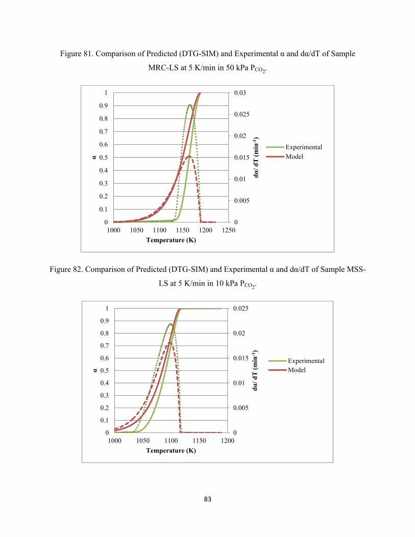
83




LS at 5 K/min in 10 kPa PCO2.

0

0.005

0.01

0.015

0.02

0.025

0.03

0

0.1

0.2

0.3

0.4

0.5

0.6

0.7

0.8

0.9

1

1000 1050 1100 1150 1200 1250

dα

/ dT

(m

in-1

)

α

Temperature (K)

Experimental

Model

0

0.005

0.01

0.015

0.02

0.025

0

0.1

0.2

0.3

0.4

0.5

0.6

0.7

0.8

0.9

1

1000 1050 1100 1150 1200

dα

/ dT

(m

in-1

)

α

Temperature (K)

ExperimentalModel

84





0

0.005

0.01

0.015

0.02

0.025

0.03

0

0.1

0.2

0.3

0.4

0.5

0.6

0.7

0.8

0.9

1

1000 1050 1100 1150 1200

dα

/ dT

(m

in-1

)

α

Temperature (K)

ExperimentalModel

0

0.005

0.01

0.015

0.02

0.025

0.03

0

0.1

0.2

0.3

0.4

0.5

0.6

0.7

0.8

0.9

1

1000 1050 1100 1150 1200 1250

dα

/ dT

(m

in-1

)

α

Temperature (K)

ExperimentalModel

85

The deviations between the experimental and predicted values ranged between 30 and

100 %, Table 14. Based on these results, it was concluded that the DTG-curve-fitting approach is

not a suitable technique to model non-isothermal calcination of limestone in CO2.

Table 14. Deviations between Predicted (DTG-SIM) and Experimental Calcination Data in CO2.

PCO2 (kPa)

MRC-LS MSS-LS

Deviation of

α (%)

Deviation of

dα/dT (%)

Deviation of

α (%)

Deviation of

dα/dT (%)

10 58.3 54.2 34.3 14.6

25 100.0 38.0 93.8 31.4

50 77.4 40.5 88.8 36.9

86

3.3.3.2 Coats-Redfern-Linearization-Based Method

The kinetic parameters obtained by the Coats-Redfern-Linearization method varied

depending on the CO2 partial pressure. The R2 values of data plotted according to the dictate of

Equation 32 were < 0.05 for an assumed n = 1. R2 > 0.999 were; however, obtained when

experimental data of sample MRC-LS (Figure 85) and sample MSS-LS (Figure 86) between

conversions 15 and 75 % were plotted according to the dictate of Equation 31 for n ≠ 1. The

corresponding activation energy and frequency factor were calculated according to Equation 35

and Equation 36 and summarized in Table 15.


CO2 Concentrations.

R² = 0.9997

R² = 0.9996R² = 0.9996

-16

-15.5

-15

-14.5

-14

-13.5

-13

0.84 0.86 0.88 0.9 0.92 0.94Ln

[ ((

1-α

)1-n

-1)

* (

n-1

)-1

* T

2

]

1000 T-1 (K-1)

MRC-LS-PCO2=10kPa

MRC-LS-PCO2=25kPa

MRC-LS-PCO2=50kPa

87


CO2 Concentrations.

Table 15. The Values of Ea, n, and A Obtained by CR-Linearization Method.

PCO2 (kPa)

MRC-LS MSS-LS

Ea A n Ea A n


10 551 2.11 E+25 1.2 633 5.37E+29 1.3

25 962 1.32 E+44 1.6 904 3.69E+41 1.7

50 1,243 3.21 E+55 2.0 1,205 5.07E+53 2.0

The activation energy varied between 551 and 1,243 kJ/mol in the ranges of CO2 pressure

employed. These values are too large for the thermal decomposition of limestone and cannot be

explained by the enthalpy of reaction and have no physical meanings. However, they present

“pseudo parameters” that can be used to predict the calcination rate of limestone in the

temperature range and the partial pressure of CO2 employed in the non-isothermal experiments.

Predicted conversion and rate of conversion data by Equation 29 and Equation 30 based on the

parameters listed in Table 15 for sample MRC-LS (Figure 87 to Figure 89) and sample MSS-LS

(Figure 90 to Figure 92) showed deviations < 6 % between the experimental and the predicted

R² = 0.9997

R² = 0.9996R² = 0.9996-16

-15.5

-15

-14.5

-14

-13.5

-13

0.84 0.89 0.94Ln

[ ((

1-α

)1-n

-1)

* (

n-1

)-1

* T

2]

1000 T-1 (K-1)

MSS-LS-PCO2=10kPa

MSS-LS-PCO2=25kPa

MSS-LS-PCO2=50kPa

88

data. The deviations were calculated using Equation 39 and are summarized in Table 16. As seen

in Figure 87 to Figure 92, the accuracies of the models decrease at near conversion > 90 %. It

should be noted that predicating the calcination rates of the limestone outside the limits of the

temperature region and CO2 partial pressure used in the experiments is not valid.


5 K/min in 10 kPa CO2.

0

0.005

0.01

0.015

0.02

0.025

0

0.1

0.2

0.3

0.4

0.5

0.6

0.7

0.8

0.9

1

1000 1050 1100 1150 1200

dα

/ dT

(m

in-1

)

α

Temperature (K)

ExperimentalModel

89





0

0.005

0.01

0.015

0.02

0.025

0.03

0

0.1

0.2

0.3

0.4

0.5

0.6

0.7

0.8

0.9

1

1000 1050 1100 1150 1200

dα

/ dT

(m

in-1

)

α

Temperature (K)

ExperimentalModel

0

0.005

0.01

0.015

0.02

0.025

0.03

0

0.1

0.2

0.3

0.4

0.5

0.6

0.7

0.8

0.9

1

1000 1050 1100 1150 1200 1250

dα

/ dT

(m

in-1

)

α

Temperature (K)

ExperimentalModel

90


K/min in 10 kPa CO2.



0

0.005

0.01

0.015

0.02

0.025

0

0.1

0.2

0.3

0.4

0.5

0.6

0.7

0.8

0.9

1

1000 1050 1100 1150 1200

dα

/ dT

(m

in-1

)

α

Temperature (K)

ExperimentalModel

0

0.005

0.01

0.015

0.02

0.025

0.03

0

0.1

0.2

0.3

0.4

0.5

0.6

0.7

0.8

0.9

1

1000 1050 1100 1150 1200

dα

/ dT

(m

in-1

)

α

Temperature (K)

ExperimentalModel

91



Table 16. Deviations between Predicted (Coats-Redfern) and Experimental Data for Sample

MRC-LS and MSS-LS.

PCO2 (kPa)

MRC-LS MSS-LS

Deviation of

α (%)

Deviation of

dα/dT (%)

Deviation of

α (%)

Deviation of

dα/dT (%)

10 2.10 5.20 1.84 5.50

25 1.07 5.75 0.89 5.16

50 0.95 5.79 0.90 5.50

3.3.3.3 Criado-Linearization-Based Method

The recarbonation reaction of lime as described by the (1-PCO2/PCO2

*) term in Equation 28

was included in data analysis using the Criado-Linearization method. The linearized plots

prepared according to the dictate of Equation 37 by assuming a reaction order to provide the best

R2 for each data set are presented in Figure 93 for sample MRC-LS and in Figure 94 for sample

0

0.005

0.01

0.015

0.02

0.025

0.03

0

0.1

0.2

0.3

0.4

0.5

0.6

0.7

0.8

0.9

1

1000 1050 1100 1150 1200 1250

dα

/ dT

(m

in-1

)

α

Temperature (K)

ExperimentalModel

92

MSS-LS. The activation energy and frequency factor calculated using Equation 35 and Equation

36 and are summarized in Table 17.

Figure 93. Criado-Linearized Plot (Equation 37) for MRC-LS Calcination at 5 K/min and

Various CO2 Concentrations.

Figure 94. Criado-Linearized Plot (Equation 37) for MSS-LS Calcination at 5 K/min and Various

CO2 Concentrations.

R² = 0.9995

R² = 0.9997R² = 0.9995

-2.5

-2

-1.5

-1

-0.5

0.84 0.86 0.88 0.9 0.92 0.94

Ln

[ ((

1-α

)1-n

-1)

* (

n-1

)-1

* T

2]

1000 T-1 (K-1)

MRC-LS-PCO2=10kPa

MRC-LS-PCO2=25kPa

MRC-LS-PCO2=50kPa

R² = 1

R² = 0.9997

R² = 0.9996

-2.1

-1.9

-1.7

-1.5

-1.3

-1.1

-0.9

-0.7

-0.5

-0.3

0.8 0.85 0.9 0.95

Ln

[ (1

-α

)-n*dα

/dt

* (1

-PC

O2/

PC

O2*

)-1

]

1000 T-1 (K-1)

MSS-LS-PCO2=10kPa

MSS-LS-PCO2=25kPa

MSS-LS-PCO2=50kPa

93

Table 17. The Values of Ea and A Obtained by Criado-Linearization Method

PCO2 (kPa)

MRC-LS MSS-LS

Ea A n Ea A n


10 278 2.32 E+12 0.55 217 5.17E+09 0.40

25 279 3.00 E+12 0.55 166 1.78E+07 0.51

50 225 6.63 E+09 0.65 255 1.29E+11 0.70

The activation energies ranged between 225 and 278 kJ/mol and they are comparable to

the values reported in the literature for the thermal decomposition of various limestone samples

in CO2 [Avila, et al., 2011]. The parameters listed in Table 17 were used to predict the

conversion and rate of conversion of each limestone according to Equation 29 and Equation 30.

The predicted data did not fit the experimental data well (Figure 95 to Figure 97 for MRC-LS

and Figure 98 to Figure 100 for MSS-LS). Deviations between the experimental and predicted

values calculated by Equation 39 were > 50 %, as shown in Table 18. Therefore, although the

Criado Linearization method is amenable to inclusion of the recarbonation reaction, the predicted

data did not fit the TGA calcination data obtained in this study.

94


at 5 K/min in 10 kPa CO2.



0

0.005

0.01

0.015

0.02

0.025

0.03

0.035

0

0.1

0.2

0.3

0.4

0.5

0.6

0.7

0.8

0.9

1

1000 1050 1100 1150 1200

dα

/ dT

(m

in-1

)

α

Temperature (K)

ExperimentalModel

0

0.02

0.04

0.06

0.08

0.1

0.12

0

0.1

0.2

0.3

0.4

0.5

0.6

0.7

0.8

0.9

1

1000 1050 1100 1150 1200

dα

/ dT

(m

in-1

)

α

Temperature (K)

ExperimentalModel

95





0

0.005

0.01

0.015

0.02

0.025

0.03

0

0.1

0.2

0.3

0.4

0.5

0.6

0.7

0.8

0.9

1

1000 1050 1100 1150 1200 1250

dα

/ dT

(m

in-1

)

α

Temperature (K)

Experimental

Model

0

0.01

0.02

0.03

0.04

0.05

0.06

0.07

0.08

0.09

0

0.1

0.2

0.3

0.4

0.5

0.6

0.7

0.8

0.9

1

1000 1050 1100 1150 1200

dα

/ dT

(m

in-1

)

α

Temperature (K)

ExperimentalModelSeries1

96



Figure 100. Comparison of Predicted (Criado) and Experimental α and dα/dT of Sample MSS-

LS at 5 K/min in 50 kPa CO2.

0

0.005

0.01

0.015

0.02

0.025

0.03

0

0.1

0.2

0.3

0.4

0.5

0.6

0.7

0.8

0.9

1

1000 1050 1100 1150 1200

dα

/ dT

(m

in-1

)

α

Temperature (K)

Experimental

Model

0

0.005

0.01

0.015

0.02

0.025

0.03

0

0.1

0.2

0.3

0.4

0.5

0.6

0.7

0.8

0.9

1

1000 1100 1200 1300

dα

/ dT

(m

in-1

)

α

Temperature (K)

ExperimentalModelSeries1

97

Table 18. Deviations between the Predicted (Criado) and Experimental Data in CO2.

PCO2 (kPa)

MRC-LS MSS-LS

Deviation of

α (%)

Deviation of

dα/dT (%)

Deviation of

α (%)

Deviation of

dα/dT (%)

10 50 68 100 100

25 100 100 100 100

50 100 100 100 100

The summary of calcination kinetic parameters and maximum deviations in the predicted

α and dα/dT using the kinetics parameters obtained by the three methods for calcination in CO2

are summarized in Table 19. Apparent kinetics parameters determined using CR method yielded

the lowest deviations between the models and experimental results.

Predicting calcination kinetics of limestone in CO2 is more complicated than in N2 in part

because the recarbonation of lime occurs and CO2 diffusional resistances in limestone/lime

particle may not be ignored. Therefore, chemical reaction is not the only rate limiting step even

at the early stage of the calcination reaction. A shrinking core model or other gas-solid reaction

models which incorporate the effects of recarbonation may need to take mass transfer limitations

into consideration to obtain improved kinetic information for the calcination of limestone in CO2.


and dα/dT for Sample MRC-LS and MSS-LS in CO2 at Various Heating Rates.

Technique Sample

PCO2

(kPa)

Ea

(kJ/mol)

A

(min-1) n

Max Deviation

(%)

DTG SIM MRC-LS 10 358 9.56 E+15 0.55 58

DTG SIM MRC-LS 25 358 5.24 E+15 0.55 100

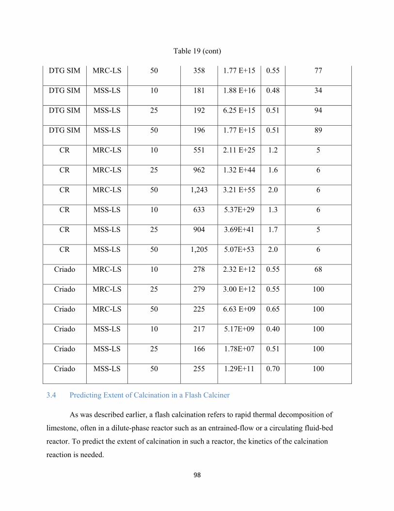
98

Table 19 (cont)

DTG SIM MRC-LS 50 358 1.77 E+15 0.55 77

DTG SIM MSS-LS 10 181 1.88 E+16 0.48 34

DTG SIM MSS-LS 25 192 6.25 E+15 0.51 94

DTG SIM MSS-LS 50 196 1.77 E+15 0.51 89

CR MRC-LS 10 551 2.11 E+25 1.2 5

CR MRC-LS 25 962 1.32 E+44 1.6 6

CR MRC-LS 50 1,243 3.21 E+55 2.0 6

CR MSS-LS 10 633 5.37E+29 1.3 6

CR MSS-LS 25 904 3.69E+41 1.7 5

CR MSS-LS 50 1,205 5.07E+53 2.0 6

Criado MRC-LS 10 278 2.32 E+12 0.55 68

Criado MRC-LS 25 279 3.00 E+12 0.55 100

Criado MRC-LS 50 225 6.63 E+09 0.65 100

Criado MSS-LS 10 217 5.17E+09 0.40 100

Criado MSS-LS 25 166 1.78E+07 0.51 100

Criado MSS-LS 50 255 1.29E+11 0.70 100

3.4 Predicting Extent of Calcination in a Flash Calciner

As was described earlier, a flash calcination refers to rapid thermal decomposition of

limestone, often in a dilute-phase reactor such as an entrained-flow or a circulating fluid-bed

reactor. To predict the extent of calcination in such a reactor, the kinetics of the calcination

reaction is needed.

99

Equation 45 is the integral form of Equation 19 when assuming isothermal conditions. It

describes the mass conversion of limestone to lime when both calcination and recarbonation

reactions are considered. The PCO2* term (the equilibrium calcination partial pressure at a given

temperature) in Equation 45 is substituted by Equation 28 to obtain Equation 46. Equation 46

can be used to calculate the EC of a limestone at a given reaction temperature and CO2 partial

pressure using the values of E, A, and n predicted from the thermal decomposition reaction of

limestone in N2.

Equation 45: ∗

Equation 46:

The extent of calcination of sample MRC-LS and sample MSS-LS were calculated using

Equation 46 (ISO T Model). The TGA kinetic parameters, determined for the thermal

decomposition of each limestone sample in N2 by the DTG-SIM method (Table 6), were used to

calculate the extent of calcination. The following assumptions were made:

1. Calcination reactor operates under an isothermal condition at atmospheric pressure

(constant calcination temperature and total pressure of 101 kPa).

2. Uniform CO2 concentration in the reactor, no radial or axial CO2 concentration gradients.

3. Limestone particles < 90 µm are rapidly heated to the calcination gas temperature. The

particle heat up time (0.1 seconds) << calcination residence time of 1 - 3 seconds (Figure

54)

4. External and intra-particle heat and mass transports are negligible.

5. Extent of calcination is not impacted by sintering and pore plugging phenomena.

6. Thermal decomposition reaction of limestone is kinetically controlled.

7. All particles are entrained in the calcination gas; thus, the residence time of a particle can

be calculated from the average gas velocity in the reactor.

100

Extent of the calcination of sample MRC-LS and sample MSS-LS calculated at different

temperatures, residence times, and partial pressures of CO2 according to Equation 46 are

presented in Figure 101 to Figure 114.

Figure 101. EC of Sample MRC-LS at 825 K.

Figure 102. EC of Sample MRC-LS at 950 K.

0

0.02

0.04

0.06

0.08

0.1

0.12

0 20 40 60 80 100 120

EC

(%

)

Time (s)

0

1

2

3

4

5

0 20 40 60 80 100 120

EC

(%

)

Time (s)

N2

10 kPa CO2

25 kPa CO2

50 kPa CO2

N2

10 kPa CO2

25 kPa CO2

50 kPa CO2

101

Figure 103. EC of Sample MRC-LS at 1,050 K.


0

10

20

30

40

50

0 20 40 60 80 100 120

EC

(%

)

Time (s)

0

5

10

15

20

25

0 2 4 6 8 10

EC

(%

)

Time (s)

N2

10 kPa CO2

25 kPa CO2

50 kPa CO2

N2

10 kPa CO2

25 kPa CO2

50 kPa CO2

102



0

10

20

30

40

50

60

0 2 4 6 8 10

EC

(%

)

Time (s)

0

20

40

60

80

100

0 2 4 6 8 10

EC

(%

)

Time (s)

N2

10 kPa CO2

25 kPa CO2

50 kPa CO2

N2

10 kPa CO2

25 kPa CO2

50 kPa CO2

103


Figure 108. EC of Sample MSS-LS at 825 K.

0

20

40

60

80

100

0 2 4 6 8 10

EC

(%

)

Time (s)

0

0.05

0.1

0.15

0.2

0.25

0.3

0.35

0 20 40 60 80 100 120

EC

(%

)

Time (s)

N2

10 kPa CO2

25 kPa CO2

50 kPa CO2

N2

10 kPa CO2

25 kPa CO2

50 kPa CO2

104

Figure 109. EC of Sample MSS-LS at 950 K.

Figure 110. EC of Sample MSS-LS at 1,050 K.

0

2

4

6

8

10

0 20 40 60 80 100 120

EC

(%

)

Time (s)

0

10

20

30

40

50

60

70

0 20 40 60 80 100 120

EC

(%

)

Time (s)

N2

50 co2

25 co2

10 co2

N2

10 kPa CO2

25 kPa CO2

50 kPa CO2

N2

10 kPa CO2

25 kPa CO2

50 kPa CO2

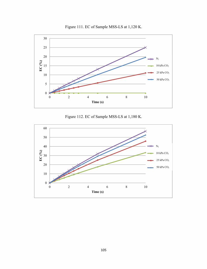
105



0

5

10

15

20

25

30

0 2 4 6 8 10

EC

(%

)

Time (s)

0

10

20

30

40

50

60

0 2 4 6 8 10

EC

(%

)

Time (s)

N2

10 kPa CO2

25 kPa CO2

50 kPa CO2

N2

10 kPa CO2

25 kPa CO2

50 kPa CO2

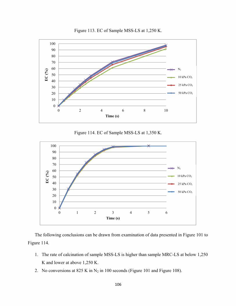
106



The following conclusions can be drawn from examination of data presented in Figure 101 to

Figure 114.

1. The rate of calcination of sample MSS-LS is higher than sample MRC-LS at below 1,250

K and lower at above 1,250 K.

2. No conversions at 825 K in N2 in 100 seconds (Figure 101 and Figure 108).

0

10

20

30

40

50

60

70

80

90

100

0 2 4 6 8 10

EC

(%

)

Time (s)

0

10

20

30

40

50

60

70

80

90

100

0 1 2 3 4 5 6

EC

(%

)

Time (s)

N2

10 kPa CO2

25 kPa CO2

50 kPa CO2

N2

10 kPa CO2

25 kPa CO2

50 kPa CO2

107

3. No conversion at 925 K in 10, 25, and 50 kPa CO2 and 100 seconds; 5 % conversion at

925 K in N2 and 60 seconds (Figure 101 and Figure 108).

4. Less than 20 % conversions at 1050 K in 10 kPa CO2 and 100 seconds (Figure 103 and

Figure 110).

5. Between 60-70 % conversions at 1,250 K in 10, 20, and 50 kPa CO2 and 5 seconds

(Figure 106 and Figure 113).

6. Conversions > 95 % at 1,350 K in 10, 20, and 50 kPa CO2 and 2.5 seconds (Figure 107

and Figure 114).

7. Increasing the temperature diminishes the impact of CO2 pressure on the calcination

reaction. Comparable conversions (83-85 %) resulted at 1,350 K in N2 and 50 kPa CO2

and 2 seconds (Figure 107 and Figure 114).

3.5 Predicting Extent of Calcination in SAP

Theoretically, ISO T Model over-estimates the extent of calcination of limestone in SAP

for several reasons. First, as was shown in Figure 115, SAP was not operated under isothermal

conditions and the gas temperature decreased along the length of the reactor. As the temperature

is lowered below the equilibrium calcination temperature, the recarbonation reaction rather than

calcination reaction will occur. However, as shown in Figure 101 to Figure 114, the ISO T

Model under estimated the extent of calcination of samples MRC-LS and MSS-LS at

temperature below 1,250 K.

Second, ISO T Model describes limestone calcination in an ideal mixed reactor where the

gas flow in uniform and mass and heat transfer transports between the limestone particles and the

calcination gas as well as intra-particle transports do not impact the calcination kinetics. In

reality; however, gas-gas and gas-solid mixing processes may not be ideal under the conditions

SAP was operated. Third, ISO T Model assumes that all of the limestone particles are entrained

in the gas and therefore the residence time of a limestone particle in SAP is equal to the average

gas residence time. However, the actual residence time of a limestone particle in the SAP

depends on its size. Therefore, the extent of calcination will be impacted by the size of the

limestone particle; residence time of a particle decreases with increasing size.

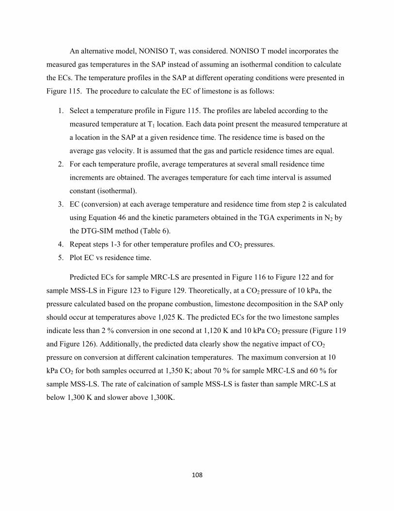
108

An alternative model, NONISO T, was considered. NONISO T model incorporates the

measured gas temperatures in the SAP instead of assuming an isothermal condition to calculate

the ECs. The temperature profiles in the SAP at different operating conditions were presented in

Figure 115. The procedure to calculate the EC of limestone is as follows:

1. Select a temperature profile in Figure 115. The profiles are labeled according to the

measured temperature at T1 location. Each data point present the measured temperature at

a location in the SAP at a given residence time. The residence time is based on the

average gas velocity. It is assumed that the gas and particle residence times are equal.

2. For each temperature profile, average temperatures at several small residence time

increments are obtained. The averages temperature for each time interval is assumed

constant (isothermal).

3. EC (conversion) at each average temperature and residence time from step 2 is calculated

using Equation 46 and the kinetic parameters obtained in the TGA experiments in N2 by

the DTG-SIM method (Table 6).

4. Repeat steps 1-3 for other temperature profiles and CO2 pressures.

5. Plot EC vs residence time.

Predicted ECs for sample MRC-LS are presented in Figure 116 to Figure 122 and for

sample MSS-LS in Figure 123 to Figure 129. Theoretically, at a CO2 pressure of 10 kPa, the

pressure calculated based on the propane combustion, limestone decomposition in the SAP only

should occur at temperatures above 1,025 K. The predicted ECs for the two limestone samples

indicate less than 2 % conversion in one second at 1,120 K and 10 kPa CO2 pressure (Figure 119

and Figure 126). Additionally, the predicted data clearly show the negative impact of CO2

pressure on conversion at different calcination temperatures. The maximum conversion at 10

kPa CO2 for both samples occurred at 1,350 K; about 70 % for sample MRC-LS and 60 % for

sample MSS-LS. The rate of calcination of sample MSS-LS is faster than sample MRC-LS at

below 1,300 K and slower above 1,300K.

109

Figure 115. Temperature Profile across SAP at Different Residence Times.

Figure 116. EC Prediction for Sample MRC-LS by NONISO T Model at T1 = 825 K.

400

600

800

1000

1200

1400

1600

0 1 2 3 4 5 6

Tem

per

atu

re (

K)

Residence Time (s)

T1=825K

T1=950K

T1=1050K

T1=1120K

T1=1180K

T1=1250K

T1=1350K

T1

T2

T3

0

0.0002

0.0004

0.0006

0.0008

0.001

0.0012

0.0014

0.0016

0.0018

0 1 2 3 4 5 6

EC

(%

)

Time (s)

Injection

N2

10 kPa CO2

25 kPa CO2

50 kPa CO2

110

Figure 117. EC Prediction for Sample MRC-LS by NONISO T Model at T1 = 950 K.

Figure 118. EC Prediction for Sample MRC-LS by NONISO T Model at T1 = 1,050 K.

0

0.005

0.01

0.015

0.02

0.025

0.03

0.035

0.04

0.045

0.05

0 1 2 3 4 5 6

EC

(%

)

Time (s)

0

0.1

0.2

0.3

0.4

0.5

0.6

0 1 2 3 4 5 6

EC

(%

)

Time (s)

N2

10 kPa CO2

25 kPa CO2

50 kPa CO2

N2

10 kPa CO2

25 kPa CO2

50 kPa CO2

111



0

0.2

0.4

0.6

0.8

1

1.2

1.4

1.6

0 1 2 3 4 5 6

EC

(%

)

Time (s)

0

0.5

1

1.5

2

2.5

3

3.5

4

4.5

5

0 1 2 3 4 5 6

EC

(%

)

Time (s)

N2

10 kPa CO2

25 kPa CO2

50 kPa CO2

N2

10 kPa CO2

25 kPa CO2

50 kPa CO2

112



0

5

10

15

20

25

0 1 2 3 4 5 6

EC

(%

)

Time (s)

0

10

20

30

40

50

60

70

80

0 1 2 3 4 5

EC

(%

)

Time (s)

N2

10 kPa CO2

25 kPa CO2

50 kPa CO2

N2

10 kPa CO2

25 kPa CO2

50 kPa CO2

113

Figure 123. EC Prediction for Sample MSS-LS by NONISO T Model at T1 = 825 K.

Figure 124. EC Prediction for Sample MSS-LS by NONISO T Model at T1 = 950 K.

0

0.0005

0.001

0.0015

0.002

0.0025

0.003

0.0035

0.004

0.0045

0 1 2 3 4 5 6

EC

(%

)

Time (s)

0

0.01

0.02

0.03

0.04

0.05

0.06

0.07

0.08

0 1 2 3 4 5 6

EC

(%

)

Time (s)

N2

10 kPa CO2

25 kPa CO2

50 kPa CO2

N2

10 kPa CO2

25 kPa CO2

50 kPa CO2

114

Figure 125. EC Prediction for Sample MSS-LS by NONISO T Model at T1 = 1,050 K.


0

0.1

0.2

0.3

0.4

0.5

0.6

0.7

0.8

0 1 2 3 4 5 6

EC

(%

)

Time (s)

0

0.2

0.4

0.6

0.8

1

1.2

1.4

1.6

1.8

2

0 1 2 3 4 5 6

EC

(%

)

Time (s)

N2

10 kPa CO2

25 kPa CO2

50 kPa CO2

N2

10 kPa CO2

25 kPa CO2

50 kPa CO2

115



0

0.5

1

1.5

2

2.5

3

3.5

4

4.5

5

0 1 2 3 4 5 6

EC

(%

)

Time (s)

0

2

4

6

8

10

12

14

16

18

20

0 1 2 3 4 5 6

EC

(%

)

Time (s)

N2

10 kPa CO2

25 kPa CO2

50 kPa CO2

N2

10 kPa CO2

25 kPa CO2

50 kPa CO2

116


Figure 130 and Figure 131 present comparisons of the experimental SAP ECs with those

predicted by the ISO T and NONISO T models at various temperatures, 5 seconds calcination

time, and 0 and 10 kPa CO2. ECs based on the two models present the maximum predicted

values at the corresponding temperatures. Both models underestimated the observed

experimental ECs at below 1,250 K and ISO T model overestimated the EC above 1,250 K.

However, both models correctly predicted no conversions below 1,025 K, the thermodynamic

calcination temperature for the thermal decomposition of the limestone in 10 kPa CO2.

Conversions in N2 (0 kPa PCO2) are also small, confirming data shown in Figure 130 and Figure

131. The fact that both limestone decomposed at below 1,025 K (EC of about 45 % at 1,025 K)

under the operating conditions of the SAP, is an indication that limestone particles were actually

exposed to much higher temperatures than measured during the SAP experiments. As was

discussed previously, temperature has the most impact on the rate of the calcination. Also, it was

mentioned earlier that experimental conversion data were presented at temperatures measured at

T1 location where the where the gas temperatures were least 10 % lower than at the location

where limestone was injected into SAP. However, even based on the temperatures at the

injection port, thermodynamically, limestone decomposition should not have occurred. Based on

the SAP results and the above discussion, it can conclude that the actual particle temperature was

likely much higher than the measured gas temperatures at the injection and T1 locations.

0

10

20

30

40

50

60

70

0 1 2 3 4 5

EC

(%

)

Time (s)

N2

10 kPa CO2

25 kPa CO2

50 kPa CO2

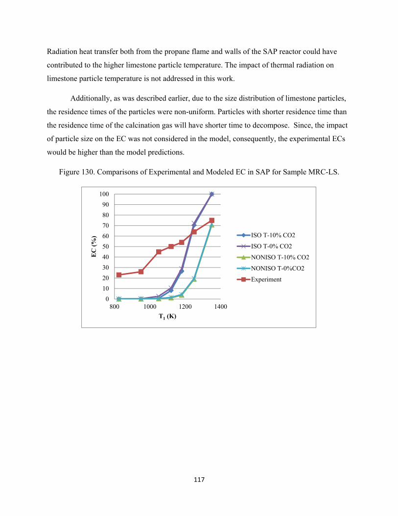
117

Radiation heat transfer both from the propane flame and walls of the SAP reactor could have

contributed to the higher limestone particle temperature. The impact of thermal radiation on

limestone particle temperature is not addressed in this work.

Additionally, as was described earlier, due to the size distribution of limestone particles,

the residence times of the particles were non-uniform. Particles with shorter residence time than

the residence time of the calcination gas will have shorter time to decompose. Since, the impact

of particle size on the EC was not considered in the model, consequently, the experimental ECs

would be higher than the model predictions.

Figure 130. Comparisons of Experimental and Modeled EC in SAP for Sample MRC-LS.

0

10

20

30

40

50

60

70

80

90

100

800 1000 1200 1400

EC

(%

)

T1 (K)

ISO T-10% CO2

ISO T-0% CO2

NONISO T-10% CO2

NONISO T-0%CO2

Experiment

118

Figure 131. Comparisons of Experimental and Modeled EC in SAP for Sample MSS-LS.

0

10

20

30

40

50

60

70

80

90

100

800 1000 1200 1400

EC

(%

)

T1 (K)

ISO T-10% CO2

ISO T-0% CO2

NONISO T-10% CO2

NONISO T-0%CO2

Experiment

119

4 SUMMARY, CONCLUSIONS AND FUTURE WORK

In this work, limestone calcination in a Sorbent Activation Process (SAP) was studied.

SAP, a patented technology, was developed by the Illinois State Geological Survey (ISGS), a

division of the Prairie Research Institute at the University of Illinois at Urbana Champaign

(UIUC) and Electric Power Research Institute (EPRI), Palo Alto, CA. SAP offers on-site

production of environmental sorbents such as activated carbon or quicklime to remove air

pollutants from flue gases of coal-fired power plants. SAP has successfully been demonstrated at

pilot- and full-scale for production of activated carbon (AC) to remove vapor-phase mercury in

coal combustion flue gas.

The focus of this research was to explore the technical feasibility of producing quicklime

from thermal decomposition of limestone in a bench-scale SAP. The bench-scale SAP located at

the Applied Research Laboratory of ISGS was used for this purpose. Pulverized limestone was

injected in the entrained-flow reactor of the SAP at different operating conditions and the

product quicklime was collected and characterized for extend of calcination and surface area.

The average calcination time varied between 3 to 5 seconds. Kinetic information for thermal

decomposition of limestone was obtained by non-isothermal thermogravimetric analysis method.

Calcination data obtained at 2, 5, and 10 K/min linear heating rates in N2 and in 10, 20, and 50

kPa CO2 were analyzed by several kinetic analysis methods to determine the reaction order,

activation energy and frequency factor at different test conditions. The kinetic information was

used to predict limestone calcination in the SAP.

SAP experiments were performed using two limestone samples (sample MRC-LS and

sample MSS-LS). Surface areas, extent of calcinations (ECs), and surface morphologies of

quicklimes produced in the SAP were significantly impacted by temperature, residence time, and

the composition of the calcination gas. Limestone calcination in the SAP occurred even at gas

temperature below 1,025 K, the minimum thermodynamic temperature for thermal

decomposition of limestone at 10 kPa CO2. It was concluded that the temperature of limestone

particles were higher than the gas temperature. Theoretically, a higher calcination temperature

and a longer residence time should result in a higher EC. Results from SAP experiments;

however, revealed that EC increased with increasing temperature field although increasing SAP

temperature resulted in decreasing the residence time of limestone particles. Therefore, it was

120

concluded that temperature field in the SAP had a stronger impact on the EC than the particle

residence time. Flash calcination in SAP suppressed the sintering effects, which causes a

decrease in surface area of quicklime, during limestone calcination due to the short exposure

time of limestone particle to the hot calcination gas. The highest total surface area was 12 m2/g

obtained from calcination of sample MRC-LS. The surface area of most commercial quicklime is

< 2 m2/g. The highest carbonate-free surface area of the lime products (normalized to its CaO

content) was 37 m2/g. EC and surface area development of limestone in SAP were independent

of particle size for smaller than 45 µm particles for the test conditions used in this research.

Kinetic parameters of calcination of limestone are required to predict calcination

behaviors in SAP. DTG-curve fitting (using DTG-SIM software), Coats-Redfern (CR), and

Criado-Linearization methods were employed to determine the kinetic parameters of calcination

of limestone samples using non-isothermal TGA data. Kinetic expressions developed using these

kinetics analysis methods predicted limestone calcination in N2 with a high accuracy (< 10 %

deviation). However, the accuracy was low (up to 100 % deviation for Criado-Linearization

method) when the same methods were applied to predict calcination of limestone in CO2. Kinetic

parameters generated using the CR-Linearization method had the smallest deviation (< 6 %)

between the experimental and predicted TGA calcination data.

Kinetic parameters obtained by the DTG-curve-fitting method in N2 were used to predict

extent of calcination in the SAP. Two different models were developed, ISO T and NONISO T.

ISO T assumes an isothermal temperature field in SAP and NONISO T uses the actual

temperature field in SAP to predict EC. The impact of mass and heat transfer limitations and

particle size distribution were not included in developing these models. The models were solely

based on chemical reaction kinetics. Model predictions showed that increasing the calcination

temperature diminishes the impact of CO2 pressure on the calcination reaction. Both models

underestimated the measured ECs in the SAP at below 1,250 K and the ISO T model

overestimated the ECs above 1,250 K. However, both models correctly predicted no conversions

below 1,025 K, the thermodynamic calcination temperature for the thermal decomposition of the

limestone in 10 kPa CO2.

Future work of this study should focus on : 1) installation of additional thermocouples to

continuously monitor both axial and radial temperature profiles in the SAP, 2) an understanding

121

of the flow pattern and hydrodynamic inside the SAP to better estimate gas-gas and gas-solid

mixing, 3) testing several size-graded limestone samples to evaluate the impact of particle size

on limestone calcination, 4) calibrating the propane and combustion air flow rates to obtain more

accurate readings, 5) quantify the extent of particle deposition in SAP, 6) measure gas phase

concentrations of CO, CO2, O2, NOx, and hydrocarbons (HCs), and verify those measured

values, and 7) incorporate mass and heat transports effects in the model to better predict

calcination performance of limestone in bench-, pilot-, and full-scale SAPs.

122

Appendix A

Equation 47 represents an unsteady-state conduction and convection heat transfer

equation for heat transfer processes from a bulk gas to a single spherical limestone particle. In

Equation 47, ρ (kg m-3), Cp (J/kg K), k (kg m-1 K-1 s-3), r (m), t (s), T (K) and Qrxn (J) denote the

density, heat capacity, conductive heat coefficient, radial location in the particle, time,

temperature of the particle at location r, and the heat consumed/release due to chemical reaction.

Radiation heat transfer by radiation is typically small compared to the convection and conduction

heat transfer; was, therefore, not included in Equation 47 [Cengel, 2007]. Although limestone

calcination is an endothermic reaction that acts as a heat sink, the heat consumed for

decomposing limestone particles was neglected because the mass of limestone injected, and

therefore the heat for thermal decomposition of the limestone, was small compared to the heat

flux from the preheated SAP and the heat provided by burning the propane. α in Equation 48

represents the Fourier thermal diffusivity (m2s-1). The dependency of T to t and r in Equation 48

can be expressed as Equation 49, where f and g represent equations which are functions of r and

t. Equation 50 is obtained when substituting Equation 49 in Equation 48, where λ is a separation

constant. Equation 50 consists of two equations, Equation 51, more commonly known as Bessel

Equation, and Equation 52. Equation 53 and Equation 54 are solutions of Equation 51, while

Equation 55 and Equation 56 are solutions of Equation 52 for different values of λ. Upon

substituting Equations 8 in Equation 49, Equation 57 is obtained, where A, B, C, and D are

arbitrary coefficients which calculated using the initial and boundary conditions presented in

Equation 58.

Equation 47:

Equation 48

Equation 49

123

Equation 50

Equation 51

Equation 52

Equation 53 if √ √

√ √

Equation 54 if √

Equation 55 if √

Equation 56 if √

Equation 57 √

√ √

The initial and boundary conditions for heat transfer process from the surrounding to the

spherical limestone particle in SAP are described in Equation 58. From Equation 58b, the

coefficient D in Equation 57 was found to be equal to T1 (Equation 59). Coefficients B and C in

Equation 57 have to be 0 for Equation 60 and Equation 58c to be valid. Zeroing B and C

coefficients, Equation 57 and Equation 60 can be rewritten as Equation 62 and Equation 63.

Substituting them in Equation 58d generates Equation 64 which upon rearranging results in

Equation 65. Combining Equation 58a and Equation 62, the coefficient A is determined in

Equation 66. Eventually, T in Equation 62 can be described as Equation 67 which can be used to

calculate temperature T at any radial position and time in the limestone particle. Heisler charts in

Figure 53 present solutions to Equation 22 in a graphical format [Heisler, 1947 and Geankoplis,

2003].

Initial and boundary conditions:

Equation 58: At t = 0 and r > 0, T = To (a)

124

At t = ∞ and r > 0, T = T1 (b)

At t > 0 and r = 0,

(c)

At r = ro π (d)

Equation 59 D = T1

Equation 60 √

√ √ √ √ √

√

Equation 61 B = C = 0

Equation 62 √

√

Equation 63 √

√ √ √

Equation 64 √

√ √

√ √

√

Equation 65 √√

Equation 66

Equation 67 √

√

Heisler Charts (Figure 53) was used to determine the temperature gradient inside a

limestone particle upon injection into the SAP reactor. In this chart, Bi, Fo, and θ*o are Biot

number, dimensionless time and temperature expressions. Biot number represents a ratio of

125

convective to conductive heat transfer as expressed in Equation 68, where ko, ro, and h represent

the heat conductivity (1.3W/m K) and radius of limestone particle (45 µm), and convective heat

coefficient in the SAP reactor (W/m2 K). Fo and α are described in Equation 69 and Equation 70,

where ρo and Cpo represent the density (2,700 kg/m3) and heat capacity of limestone (840 J/kg

K). θo* is defined in Equation 71, where To, T1, and T represent the initial temperature of the

limestone particle (300 K), gas temperature in SAP, and temperature at the center of the

limestone particle. Convective heat coefficient was calculated using the correlation for flow past

a single sphere (Equation 72). In Equation 72, Rep and Pr represent Reynolds number for

limestone particle (Equation 73) and Prandtl number (Equation 74), where ρ, k, µ, and Cp

represent the density, thermal conductivity, viscosity, heat capacity of the gas, while Do

represents the diameter of the limestone particle (80 µm). CHEMCAD was used to determine the

properties of flue gas based on stoichiometric propane combustion. The properties of gas were

evaluated at Tf which represents the average temperature between bulk gas and limestone

particle temperature initially as defined in Equation 75.

Equation 68 .

Equation 69

Equation 70

Equation 71 ∗

Equation 72 . . .

Equation 73

Equation 74 .

Equation 75

126

REFERENCES

Adolfsson, E, Nygren, M, and Hermansson, L. Decomposition mechanisms in aluminum oxide

apatite systems." Journal of American the Ceramic Society 82, 2909-2912 (1999).

Ar, I. Calcination kinetics of high purity limestones. Chemical Engineering Journal 83, 131-137

(2001).

Avila, I, Crnkovic, P.M., Milioli, F. E., and Luo, K.H. Thermal decomposition kinetics of

Brazilian limestones: effect of CO2 partial pressure. Environmental Technology 1, 1-8

(2011).

Baker, E.H. The calcium oxide – carbon dioxide system in the pressure range 1 – 300

atmospheres. Journal of the Chemical Society 0, 464 – 470 (1962).

Benson, L.B., Smith, K. J., Roden, R. A., Loch, E., Potts, J. Control of Sulfur Dioxide and Sulfur

Trioxide Using By-Product of a Magnesium-Enhanced Lime FGD System. paper

presented at the Institute of Clean Air Company ICAC Forum 2003: Multi-Pollutant

Emission Control & Strategies, Nashville, TN (2003).

Beruto, D. and Searcy, A.W. Use of the Langmuir method for kinetic studies of decomposition

reactions: calcite (CaCO3). Journal of the Chemical Society Faraday Transactions 1 70,

2145 (1974).

Biarnes, M. "Combustion." E-Instrument. Web. (accessed April, 2012).

<http://www.e-inst.com/docs/E-Instruments-Combustion-Booklet-2009.pdf>.

Borgwardt, R.H. Kinetics of the reaction of sulfur dioxide with calcined limestone.

Environmental Science & Technology 4, 59-63 (1970).

Borgwardt, R.H. and Harvey, R.D. Properties of carbonate rocks related to sulfur dioxide

reactivity. Environmental Science & Technology 6, 350-360 (1972).

Borgwardt, R.H. Calcination kinetics and surface area of dispersed limestone particles. American

Institute of Chemical Engineers Journal 31, 103-111 (1985).

127

Borgwardt, R.H. and Bruce, K.R. Effect of specific surface area on the reactivity of CaO with

SO2. American Institute of Chemical Engineers Journal 32, 239-246 (1986).

Borgwardt, R.H. Sintering of nascent calcium oxide. Chemical Engineering Science 44, 53-60

(1989).

Borgwardt, R.H. Calcium oxide sintering in atmospheres containing water and carbon dioxide.

Industrial & Engineering Chemistry Research 28, 493-500 (1989).

Boynton, R. S. Chemistry and Technology of Lime and Limestone. John Wiley & Sons.

ISBN 0-471-02771-5 (1980).

British Lime Association. “How a Kiln Works.” Web. (accessed June, 2011).

<http://www.britishlime.org/edu_kiln01.php>.

Campbell, F.R., Hills, A.W.D. and Paulin, A. Transport properties of porous lime and their

influence on the decomposition of porous compacts of calcium carbonate. Chemical

Engineering and Science, 25 929–942 (1970).

Campbell, J.H. Kinetics of Decomposition of Colorado Oil Shale: II. Carbonate Minerals.

Lawrence Livermore National: Livermore, CA. UCRL-52089 2, 53 (1978).

Cengel, Y.A. Heat and Mass Transfer: A Practical Approach. McGraw-Hill. ISBN 0-071-52739-

X (2007).

Chan, R. K., Murthi, K. S., and Harrison, D. Thermogravimetric analysis of Ontario limestones

and dolomites. 11. reactivity of sulfur dioxide with calcined samples. Canadian Journal

of Chemical Engineering, 48 2979 (1970).

Chang, R, Rostam-Abadi, M., and Chen, S. Apparatus and Method for Removal of Vapor Phase

Contaminants from a Gas Stream by In-situ Activation of Carbon-based Sorbents.

Electric Power Research Institute, Inc. (Palo Alto, CA), assignee. Patent 6,451,094

(2002).

Chang, R, Rostam-Abadi, M., and Sjostrom, S. Method for Removal of Vapor Phase

Contaminants from a Gas Stream by In-situ Activation of Carbon-based Sorbents.

128

Electric Power Research Institute, Inc. (Palo Alto, CA), assignee. Patent 6,558,454

(2003).

Chang, R., Lu, Y., and Rostam-Abadi, M. Method and Apparatus for On-Site Production of

Lime and Sorbents for Use in Removal of Gaseous Pollutants. Electric Power Research

Institute, Inc. (Palo Alto, CA), assignee. Patent 20,110,223,088 (2011).

Chen, X. "Impacts of Fly Ash Composition and Flue Gas Components on Mercury Speciation."

Diss. University of Pittsburgh. 2007. Web. (accessed March, 2012)

<http://d-scholarship.pitt.edu/8590/1/ChenX_ETD_2007.pdf. >

Cheng, C. and Specht, E. Reaction rate coefficients in decomposition of lumpy limestone of

different origin. Thermochimica Acta 449, 8-15 (2006).

Cooper, D. C. and Alley, F. C. Air Pollution Control: A Design Approach. 3rd ed. Waveland

Press, Inc (2002).

Criado, J.M., Gonzalez, M., Tlek, J. M., and Ortega, A. The effect of the CO2 pressure on the

thermal decomposition kinetics of calcium carbonate. Thermochimica Acta 254, 121-127

(1995).

Daoudi, M. and Walters, J. K. The reaction of HCl gas with calcined commercial limestone

Particles: the effect of particle size. Journal of Chemical Engineering 47, 11-16 (1991).

Energy Information Administration (EIA). US Coal Reserves: An Update by Heat and Sulfur

Content. U.S. Department of Energy. Washington: DOE/EIA-0529(92) (1993).

Elder, J. P. and Reddy, V. B. The Kinetics of the Thermal Degradation of Calcium

Carbonate. Journal of Thermal Analysis 31, 395-405 (1986).

Electric Power Research Institute (EPRI). “On-Site Sorbent Activation for Mercury Control at

Coal-Fired Power Plants.” Web. (accessed May, 2010).

<http://mydocs.epri.com/docs/TI/1021633_Sorbent%20Activation_v3.pdf>.

Everson, R.C., Neomagus, H.W.J.P., and Njapha, D. Kinetic analysis of non-isothermal

thermogravimetric analyser results using a new method for the evaluation of the

temperature integral and multi-heating rates. Fuel 85, 418-422 (2006).

129

Feeley III, T.J., et al. An update on DoEʼs phase II and phase III mercury control technology

R&D program. Fuel Processing Technology 90, 1388-1391 (2009).

Fluke. "Fluke 50 Series II Thermometers." Web. (accessed January, 2012).

<http://www.fluke.com/fluke/usen/electrical-test-tools/thermometers/fluke-50-series-

ii.htm?PID=56085>.

Fonseca, A.M., Órafäo, J.J., and Salcedo, R.L. A new approach to the kinetic modeling of the

reaction of gaseous HCl with solid lime at low temperature. Chem. Eng. Science 58,

3499–3506 (2003).

Fonseca, A.M., Órafäo, J.J., and Salcedo, R.L. Kinetic modeling of the reaction of HCl and solid

lime at low temperatures. Ind. Eng. Chem. Res 37, 4570–4576 (1998).

Fuertes, A. B., Alvarez, D., Rubiera, F., Pis, J. J., and Marban, G. Simultaneous calcination and

sintering model for limestone particles decomposition. Transactions of the Institution of

Chemical Engineers, 71A, 69–76 (1993).

Geankoplis, C. J. Transport Processes and Separation Process Principles: (Includes Unit

Operations). 4th ed. New Delhi: Prentice Hall of India, 373-74 (2003).

German, R.M. and Munir, Z.A. Surface area reduction during isothermal sintering. Journal of the

American Ceramic Society 59, 379–383 (1976).

GXT, Inc. "FERRET 16 Emissions Analyzer." Web. (Apr, 2012).

<http://www.gxtauto.com/uploads/16-Flyer.pdf>.

Hartman, M., Pata. J., and Coughlin, R. W. Influence of porosity of calcium carbonates on their

reactivity with sulfur dioxide. Industrial & Engineering Chemistry Process Design and

Development 17, 411-419 (1978).

Hartman, M. and Trnka, O. Reactions between calcium oxide and flue gas containing sulfur

dioxide at lower temperatures. American Institute of Chemical Engineers Journal 39,

615-624 (1993).

Heisler, M. P. Temperature charts for induction and constant temperature heating, Trans. ASME

69, 227–236, (1947).

130

Hills, A.W.D. The mechanism of the thermal decomposition of calcium carbonate. Chemical

Engineering Science 23, 297-320 (1968).

Hoffmann, J., and Ratafia-Brown, J. Preliminary cost estimate of activated carbon injection for

controlling mercury emissions from an un-scrubbed 500 MW coal-fired power plant.

final report for DoE - National Energy Technology Laboratory - Innovations for Existing

Plant Program. (2003).

HORIBA. “Compact Laser Diffraction Particle Size Analyzer LA-300.” Web. (accessed June,

2011).

<http://www.horiba.com/us/en/scientific/products/particle-characterization/particle-size-

analysis/details/la-300-110/>.

Hsi, H.C., Rood, M.J., Rostam-Abadi, M., Chen, S., and Chang, R. Effects of sulfur

impregnation temperature on the properties and mercury adsorption capacities of

activated carbon fibers (ACFs). Environmental Science & Technology 35, 2785-2791

(2001).

Hu, N. and Scaroni, A.W. Calcination of pulverized limestone particles under furnace injection

conditions. Fuel 75, 177-186 (1996).

Hyatt, E.P., Cutler, I.B., and Wadsworth, M.E. Calcium carbonate decomposition in carbon

dioxide atmosphere. Journal of American the Ceramic Society 41, 70–74 (1958).

Ingraham, T.R. and Marier, P. Kinetic studies on the thermal decomposition of calcium

carbonate. Canadian Journal of Chemical Engineering 41, 170–173 (1963).

Irabien, A., Cortabitarte, F., and Ortiz, M. I. Kinetics of Flue Gas Desulfurization at Low

Temperatures: Nonideal Surface Adsorption Model. Chemical Engineering and Science

47, 1533 (1992).

Keener, S. and Kuang, S.J. Structural pore development model for calcination. Chemical

Engineering Communications 117, 279-291 (1992).

131

Khinast, J., Brunner, C., Aichinger, G., and Staudinger, G. Reaction during Low Temperature

Dry Flue Gas Desulfurization. paper presented at the 15th SO2 Control Symposium

(1995).

Khinast, J., Krammer, G., and Brunner, C. Decomposition of limestone: the influence of CO2 and

particle size on the reaction rate. Chemical Engineering 51, 623-634 (1996).

Kidde. "Carbon Monoxide Alarms and Combo Alarms AC Plug-in Operated : Model KN-COPP-

3." Web. (accessed April, 2012).

<http://www.kidde.com/utcfs/Templates/Pages/Template53/0,8062,pageId%3D4428%26

siteId%3D384,00.html>.

Klingspor, J., Karlsson, H. T., and Bjerle, I. A kinetic study of the dry SO2-limestone reaction at

low temperature. Chemical Engineering Communications 22, 81-103 (1983).

Kocaefe, D., Karman, D., Steward, F. R. Comparison of the sulfation rates of calcium,

magnesium and zinc oxides with SO2 and SO3. Canadian Journal of Chemical

Engineering 63, 971-977 (1985).

Lee, S.F., Seo, Y.C., Jongsoo, J., and Lee, T.G. Removal of gas-phase elemental mercury by

iodine- and chlorine-impregnated activated carbons. Atmospheric Environment 38, 4887-

4893 (2004).

Lee S.H. and Park Y.O. Gas-phase mercury removal by carbon-based sorbents. Fuel Processing

Technology 84, 197–206 (2003).

Likens, G. “Acid Rain". Encyclopedia of Earth. Web. (accessed December, 2010).

<http://www.eoearth.org/article/Acid_rain?topic=49506>.

Liu, C. F. and Shih, S. M. Kinetics of the reaction of hydrated lime with SO2 at low

temperatures: effects of the presence of CO2, O2, and NOx. Industrial & Engineering

Chemistry Research 47 (2008).

Milne, C.R., Silcox, G.D., Pershing, D.W., and Kirchgessner, D.A. Calcination and sintering

models for application to high-temperature, short-time sulfation of calcium-based

sorbents. Industrial & Engineering Chemistry Research 29, 139-149 (1990).

132

Quantachrome. "Monosorb B.E.T Surface Area Analyzer." Web. (accessed May, 2011).

<http://www.quantachrome.com/gassorption/monosorb.html>.

Morris, L. “Acid Gas Emission Control Measures.” Web. (accessed June, 2011).

<http://www.pennenergy.com/index/power/display/9915040467/articles/power-

engineering/volume-114/issue-10/features/acid-gas-emission-control-measures.html>.

Morrison, A. F. Data correlation for drag coefficient for sphere. Department of Chemical

Engineering, Michigan Technological University, Houghton, MI. 2010. (accessed April,

2012).

<www.chem.mtu.edu/~fmorriso/DataCorrelationForSphereDrag2010.pdf>

Oates, J. A. H. Lime and Limestone: Chemistry and Technology, Poduction and Uses.

Weinheim: Wiley-VCH (1998).

Ohme, K., Schrader, R. and Müller, A. Kinetik der thermischen dissoziation von kalkstein und

zementrohmehl im flugstaubreaktor. Silikattechnik 26, 403–407 (1975).

Powell, E. K. and Searcy, A. W. Surface areas and morphologies of CaO produced by

decomposition of large CaCO3 crystals in vacuum. Communications of the American

Ceramic Society 42-44 (1982).

Rochelle, G. Reaction of Hydrated Lime with SO2 in Humidified Flue Gas. paper presented at

SO2 Control Symposium EPA/EPRI, New Orleans, LA (1990).

Schenelle, K.B. and Brown, C.A. Air Pollution Control Technology Handbook. CRC Press LLC.

Boca Raton, FL (2002).

Schenck. “AccuRate Dry Material Feeder." Web. (accessed March, 2012).

<http://www.genemco.com/catalog/pdf/SNSL272accuratefeeder.pdf>.

SIGRIST. "Isokinetic Sample." SIGRIST Process Photometer. Web. (accessed April, 2012).

<http://www.photometer.com/en/abc/show.html?q=Isokinetic%20sample>.

Silcox, G.D., Kramlich, J.C., and Pershing, D.W. A mathematical model for the flash calcination

of dispersed calcium carbonate and calcium hydroxide particles. Industrial &

Engineering Chemistry Research 28, 155-160 (1989).

133

Singh, N. B., and Singh, N. P. Formation of CaO from thermal decomposition of calcium

carbonate in the presence of carboxylic acids. Journal of Thermal Analysis and

Calorimetry 89, 159-62 (2007).

Sjostrom S., Wilson, C., Bustard, J., Spitznogle, G., Toole, A., O’Palko, A., Chang, R. Full-scale

Evaluation of Carbon Injection for Mercury Control at a Unit Firing High Sulfur Coal.

ADA-ES, Inc – American Electric Power Corporation – DoE – EPRI. paper presented at

USEPA – DoE – EPRI Combined Power Plant Air Pollutant Control Symposium: The

MEGA Symposium. Baltimore, Maryland (2006).

Smith, D. “SO2 Controls: Cost of Scrubbers Down to $100/kW”. Power Engineering. 2001.

Web. (accessed April, 2012).

<http://www.power-eng.com/articles/print/volume-105/issue-9/features/sosub2-sub-

controls-cost-of-sosub2-sub-scrubbers-down-to-100-kw.html>

Thermo Scientific. "Thermo Scientific TGA VersaTherm Analyzer." Web. (accessed March,

2012).

<http://www.reoterm.com.br/central/Analise_Termica/VersaTherm%20TGA.pdf>.

Thibault, J. D., Steward, F. R., and Ruthven, D. M. The kinetics of absorption of SO3 in calcium

and magnesium oxides." Canadian Journal of Chemical Engineering 60, 796-801 (1982).

Thompson, J.L. Prediction lime burning rate via new dynamic calcination theory. Pit and Quarry

5 (1979).

USEPA. "Mercury and Air Toxics Standards (MATS) for Power Plants." Web (accessed March,

2012a). <http://www.epa.gov/mats/basic.html>.

USEPA. “Air Pollution Control Technology Fact Sheet.” Publication no. EPA-452/F-03-034.

Web (accessed March, 2012b).

<http://www.epa.gov/ttncatc1/dir1/ffdg.pdf>.

USEPA. “Health Effects of Mercury.” Web (accessed March, 2012c).

<http://www.epa.gov/hg/effects.htm>.

134

Wark, K., Warner, C.F., and Davis, W.T. Air Pollution: Its Origin and Control. Addison-Wesley.

Menlo Park, CA (1998).

Yan, R., Chin, T., Liang, D. T., Laursen, K., Ong, W. Y., Yao, K., and Tay, J. H. Kinetic study

of hydrated lime reaction with HCl. Environmental Science & Technology 37, 2556-2562

(2003).

Yang, J., Miranda. R., and Roy, C. Using the DTG curve fitting method to determine the

apparent kinetic parameters of thermal decomposition of polymers. Polymer Degradation

and Stability 73, 455-461 (2001).

Yu, H. D., Zhang, Z. Y., Win, K. Y., and Chan, J. Bioinspired fabrication of 3D hierarchical

porous nanomicrostructures of calcium carbonate for bone regeneration. Chemical

Communications 46, 6578-6580 (2010).

Zhuang, Y., Olson, E., and Galbreath, K. Mercury transformations in coal combustion flue gas.

Fuel Processing Technology 65-66, 289-310 (2000).

Zhuang, Y., Martin, C., Pavlish, J., and Botha, F. Cobenefit of SO3 reduction on mercury capture

with activated carbon in coal flue gas. Fuel 90, 2998-3006 (2011).

Zhong, Q. and Bjerle, I. Calcination kinetics of limestone of nascent CaO. Thermochimica Acta

223, 109-120 (1993).

flash calcination of limestone in a bench-scale sorbent

Documents