flow patterns in inclined gas-liquid annular duct flow · flow patterns in inclined gas-liquid...

Flow patterns in inclined gas-liquid annular duct flow

F. A. A. Mendes1, O. M. H. Rodriguez1, V. Estevam2 & D. Lopes3 1Department of Mechanical Engineering, Engineering School of São Carlos, University of São Paulo (USP), Brazil 2PETROBRAS/E&P-ENGP/TPP/EE, Brazil 3PETROBRAS/UN-RIO/ENGP/EE, Brazil

Abstract

The submergible centrifugal pump (SCP) is one of the most common artificial lifting techniques employed in the Brazilian offshore scenario. However, free gas in the suction of the SCP is one of the most important limitations in the design of the pumping system. Gas-liquid flow in annular-ducts is found in the petroleum industry associated with gravitational gas separators that are applied with the SCP technique for oil production in directional wells. The main goal of this study is to investigate the behavior, i.e., flow patterns and maps, of gas-liquid flow in an annular duct at several inclinations in a setup with dimensions which are closer to real offshore application. High-speed video recording together with an objective technique based on the time-frequency pressure-signature analysis were applied for the flow pattern characterization. The experimental data were collected in the apparatus consisted of an inclinable test section, 0 to 90 degrees, with inner and outer diameters of 75 mm and 111 mm, respectively, hence the annular channel possessing an 18 mm gap. The total length of the test section was of 10.5 m. Air, water and oil at near atmospheric pressure constituted the gas and liquid phases. The air, water and oil superficial velocities were in the range of 0.02–30 m/s, 0.02–5 m/s and 0.005–0.5 m/s, respectively. Comparisons between data and flow pattern maps available in the literature for annular duct allowed the discrimination of regions and flow situations for which improvements of the transition modelling are required. Keywords: two phase flow, annular duct, flow patterns maps, time-frequency pressure signature, directional well, inclined flow.

Computational Methods in Multiphase Flow VI 271

www.witpress.com, ISSN 1743-35 (on-line) WIT Transactions on Engineering Sciences, Vol 70, © 2011 WIT Press

33doi:10.2495/MPF110 123

1 Introduction

The multiphase flow in annular-duct can be found frequently in the oil industry; however, little is known about the phenomenology of this flow type. This knowledge is important for the design of submergible centrifugal pump (SCP). The SCP is one of the most common artificial lifting techniques employed in the Brazilian offshore scenario. In addition, free gas in the suction of the SCP is one of the most critical limitations in the design of the pumping system. Gas-liquid flow in annular-ducts is found in the petroleum industry associated with gravitational gas separators that are applied with the SCP technique for oil production in directional wells. Kelessidis and Dukler [1] presented a study on upward-vertical two-phase flow in an annular duct. The authors traced flow patterns maps and established the transitions of flow patterns experimentally. Hasan and Kabir [2] proposed a phenomenological model for transitions in upward vertical and inclined annular duct flow and used data from the literature to validate the model. Caetano et al. [3] carried out an experimental and theoretical study of the effect of eccentricity in an upward-vertical two-phase annular-duct flow. The only quoted authors who studied the influence of inclination on flow patterns was Hasan and Kabir [2], however the model was validated only with data of upward-vertical flow. The studies [4] and [5] show results for horizontal two-phase annular-duct flow. In the first study, the authors were looking for the effect of slope on flow patterns, while in the second study the air-water flow patterns were classified and compared in two different sections test. In both studies, they used small tubes (annular channel gap of about 1 mm), which is not compatible with the dimensions used by the oil industry. Furthermore, the authors have not proposed any model for flow pattern transition. An objective identification and characterization of flow patterns based on statistical analysis of time-frequency pressure fluctuation signal was proposed by Drahos et al. [6] and Matsui [7]. Drahos et al. [6] used an analysis of the PDFs (Probability density function) and PSDs (Power Spectrum Density) to identify and characterize the flow patterns in a gas-liquid two-phase flow in a horizontal pipe. Matsui [7] applied statistical tools for analyzing the PDF of the differential pressure signals in vertical gas-liquid two-phase pipe flow. Blanco et al. [8] conducted a thorough review on the study of gas-liquid flow in annular duct and proposed flow patterns maps for the annular-duct flow in horizontal and vertical inclinations. However, those authors don't validated the proposed model with data related to dimensions similar to those found in the oil industry because of the lack of available data in the literature. The main purpose of this study is to expand the existing experimental database on two-phase flow in annular ducts and validate the phenomenological model proposed by Blanco et al. [8].

272 Computational Methods in Multiphase Flow VI


33

2 Experiments

2.1 Experimental apparatus

The experimental data were obtained from the experimental apparatus illustrated by fig. 1. This experimental apparatus is mounted in Thermal-Fluids Engineering Laboratory (NETeF) of the Engineering School of São Carlos of the University of São Paulo. The test section (TS) has an annular geometry and is made of borosilicate glass. It has 10.5 m of length and is sustained by an inclinable truss beam capable of going from horizontal to 90 degrees of inclination. There is a flow development section of 1.5 m and 111 mm of internal diameter before the annular duct of 7.5 m and 111 mm of outside diameter (Do) and 75 mm of internal diameter (Di), fig. 2. A pipe section identical to the development section was positioned after the annular test section.

Figure 1: Schematic of experimental apparatus.

The air is supplied by a Worthington screw compressor of 50 kW model ROLLAIR 40 (SC), whose flow control is done by needle valves positioned before the flow meters. Three orifice plates (AF1, AF2, AF3) and an Oval positive displacement flow meter model Gal 50 (AF4) are used for measuring the air flow. The tap water used in test is pumped from a water tank (WR) by a Weatherford progressive cavity helical pump of 11kW model WHT (WP). To measure the water flow it is used a Badger Meter positive displacement flow meter OGT (WF1) and an Oval vortex water flow meter model EX Delta. The oil (density 828 kg/m³, viscosity 0,22 Pa.s and superficial tension oil-ar 52x10-3 N/m

SC

TS1

PT1

PT4

PT3

PT2

PT5

TS2

TS3

TS4

TS5

AR

WR

OR

WP

OP

OF1 OF2

WF1 WF2

AF1

AF3

AF2

AF4

AFi

GL-M

GL-S

OW-S

PT6

DPT

TS

TG

VS



33

at 25C) is pumped by a Weatherford progressive cavity helical pump of 11kW model WHT (OP). Two Oval positive displacement flow meters are used to measure the oil flow: MIII (OF1) and Flowpet EG (OF2). The gas-liquid mixture is formed in the gas-liquid mixer (GL-M), it is separated in the gas-liquid separator (GL-S) and the air is vented to the atmosphere. The liquid returned by gravity to tank (WR) or (OR). Novus pressure transducers TP-150 with range of 0-5 bar, accuracy 0,5% (PT2, PT3, PT4, PT5,PT6) were used to measure pressure and IOPE temperature sensor model TW-TC/2 (TS1, TS2, TS3, TS4, TS5), range -20–140C and accuracy 0,5C were used to measure temperature. Tab. 1 summarizes the measurements instruments used in this study.

Table 1: Measurement instruments.

Flow meter Range at 1 atm and 25C (l/min) Accuracy AF1 57–262 1% RD AF2 172–794 1% RD AF3 524–2400 1% RD AF4 1–20 +1% -5% RD OF1 0,05–8 1% RD OF2 2,5–106 1% RD WF1 1–35 1% RD WF2 30–1300 1% RD

An Optron is high speed camera model CamRecord 600 is positioned in front of the visualization section (VS) and used to capture images of the flow. Xenon lamps of 35 W and 6000 K are positioned so as to provide sufficient lighting to obtain the images, fig. 3. A Validayne differential pressure transducer, model DP-15 (DPT) is used to acquire the two-phase flow pressure signature. At the entrance of the acquisition system it is installed a low-pass filter of 20 Hz to eliminate the signal noise of the pressure transducer. The remote control and acquisition system consisted of a PC equiped with a National Instruments acquisition board model PCI-6224. The water pump is controled with the assistance of a CAM system. The inclination angle of the test section (TS) is measured with a Bosh angle meter DNM 60L, accuracy 0,2.

2.2 Experimental procedure

The test section (TS) was set to the desired angle. The liquid superficial velocity was established by the pump control system using a PID controller implemented in LabView™ platform. The air injection was controlled manually through the needle valves. After five minutes, which was enough time to ensure steady state, the signal provided by the pressure transducer was saved and the image acquisition performed for a period of 60 s. The flow-pattern transition boundaries were determined a posteriori by visual observations (subjective technique) and the signal analysis (objective technique) based on the Fourier transform (FFT) and the Probability density function (PDF) of the pressure signature.



33

Figure 2: Schematic of the test section.

Figure 3: High-speed camera setup.

3 Results and discussion

3.1 Subjective analysis

In the subjective analysis the movies of the flow were carefully analyzed in slow motion, which allowed the identification and characterization of the flow patterns. Fig. 4 illustrates the horizontal water-air wavy stratified flow pattern obtained at an acquisition rate of 1000 fps and resolution of 800 x 500 pixels. The superficial velocities were set at JG=10.26 m/s and JL=0.25 m/s m/s. The four snapshots show an interfacial wave crossing the visualization section.

0 s 0,12 s

0,18 s 0,24 s

Figure 4: Lateral view of wavy stratified flow (JG=10.26 m/s e JL=0.25 m/s); Di stands for internal diameter.

Fig. 5 illustrates an elongated bubble observed from above during plug flow. One can see the deformed bubble due to the annular geometry. The bubble takes on a form that resembles of a flatworm. The lateral view of a “flatworm” bubble crossing the visualization section during plug flow can be seen in fig. 6. The camera was set to an acquisition rate of 1000 fps and a resolution of 800 x 500 pixels. The air and water superficial velocities were JG=0,25 m/s and JL=3,52 m/s.

Di

Do

Di



33

Figure 5: Top view of an elongated “flatworm” bubble in plug flow.

0 s 0,1 s

0,2 s 0,3 s

Figure 6: Lateral view of a “flatworm” bubble in plug flow; JG=0.25 m/s and JL=3.52 m/s.

0 s 0,05 s 0,14 s

0,22 s 0,28 s 0,34 s

Figure 7: Lateral view of slug flow; JG=2 m/s and JL=1.25 m/s.

Fig. 7 shows a sequence of images of the slug flow pattern, JG=2 m/s and JL=1,25 m/s, with the camera set at an acquisition rate of 1000 fps and 800 x 500 pixels. The first snapshot (t = 0 s) shows a smooth stratified flow pattern. The following five snapshots show the aerated water slug crossing the visualization section. Notice that at t = 0.34 s the flow resembles an aerated wavy stratified flow. A picture of the dispersed bubble flow pattern is shown by Fig. 8. The

Di

Di

Do

Di



33

Figure 8: Lateral view of dispersed bubble flow, JG=0.05 m/s e JL=4.38 m/s.

sequence of images was carried out at a rate of 1250 fps and a resolution of 1280 x 256 pixels. The superficial velocities were JG=0.05 m/s e JL=4.38 m/s.

3.2 Objective analysis

The Validyne differential pressure transducer was mounted with diaphragm 20 (pressure range of -860 to 860 Pa) to identify the stratified flow and diaphragm 32 (pressure range of -14 to 14 kPa) for all the other flow patterns. Data were acquired at a rate of 5 kHz, with an accuracy of 0.25% FS and analyzed by a homemade program implemented in LabView™.

3.2.1 Horizontal flow Air-water. Figs. 9–12 illustrates the acquired signal in time and frequency domains related to air-water smooth stratified flow, wavy stratified flow, slug flow and dispersed bubble flow, respectively. The basic difference between slug flow (fig.11) and plug flow (fig.12) is the observed intermittence of the signal in time. In addition, it is clear from the PSD graph that for plug flow the frequency peak is in between that of stratified flow and dispersed bubble flow. In stratified flow the dominant frequency is around 1 Hz, while in plug flow it is around 2 Hz and in dispersed bubble flow it is above 4 Hz. In the time domain, the smoothness of the signal is a clear discriminator between smooth (fig. 10) and wavy (fig. 11) stratified flow. In addition, the PSD of the smooth stratified flow signal presents a narrower frequency range than that of wavy stratified flow. The slug flow signal is characterized by strong pulsation in time (fig. 12). It indicates the passage of the piston of liquid that is formed by Kelvin-Helmholtz instability. The main feature of the signal related to dispersed bubble flow is the existence of a well defined high frequency oscillation (fig. 13). Air-oil. One can see in Figs. 14 and 15 the signals related to smooth and wavy stratified flow in the tests with air and oil. In the frequency domain, the smooth stratified flow signal shows essentially a single low oscillation frequency (fig. 14), whereas the signal related to wavy stratified flow (fig. 15) presents a higher and broader distribution of frequencies in the PSD graph. The intermittent flow is divided in slug and plug flow. The signal related to plug flow (fig. 17)

Signal

PSD

Figure 9: Smooth stratified flow (JG=0.05 m/s; JL=0.05 m/s).

0 2 4 6 8 10 12 14 16 18 20 22 24 26 28 30 32 34 36 38 40 42 44 46 48 50 52 54 56 58 60-2000

-1500

-1000

-500

0

500

1000

1500

2000

P (

Pa)

Tempo (s)0 1 2 3 4 5 6 7 8 9 10 11 12 13 14 15 16 17 18 19 20

0,0

5,0x10-2

1,0x10-1

1,5x10-1

2,0x10-1

2,5x10-1

3,0x10-1

3,5x10-1

PS

D

Frequência (Hz)

Di

Do



33

Signal

PSD

Figure 10: Wavy stratified flow (JG=5.00 m/s; JL=0.20 m/s).

Signal PSD

Figure 11: Slug flow (JG=3 m/s; JL=2 m/s).

Signal

PSD

Figure 12: Plug flow (JG=0.1 m/s; JL=1 m/s).

Signal

PSD

Figure 13: Dispersed bubble flow (JG=0.05 m/s; JL=4.00 m/s).

Signal

PSD

Figure 14: Smooth stratified flow (JG=0,1 m/s; JL=0,03 m/s).

Signal

PSD

Figure 15: Wavy stratified flow (JG=15,00 m/s; JL=0,06 m/s).

0 2 4 6 8 10 12 14 16 18 20 22 24 26 28 30 32 34 36 38 40 42 44 46 48 50 52 54 56 58 60-2000

-1500

-1000

-500

0

500

1000

1500

2000

P (

Pa)

Tempo (s)0 1 2 3 4 5 6 7 8 9 10 11 12 13 14 15 16 17 18 19 20

0,0

2,0x101

4,0x101

6,0x101

8,0x101

1,0x102

PS

D

Frequência (Hz)

0 2 4 6 8 10 12 14 16 18 20 22 24 26 28 30 32 34 36 38 40 42 44 46 48 50 52 54 56 58 60-2000

-1500

-1000

-500

0

500

1000

1500

2000

P (

Pa)

Tempo (s)

0 1 2 3 4 5 6 7 8 9 10 11 12 13 14 15 16 17 18 19 20

0,0

5,0x102

1,0x103

1,5x103

2,0x103

2,5x103

3,0x103

PS

D

Frequência (Hz)

0 2 4 6 8 10 12 14 16 18 20 22 24 26 28 30 32 34 36 38 40 42 44 46 48 50 52 54 56 58 60-2000

-1500

-1000

-500

0

500

1000

1500

2000

P (

Pa)

Tempo (s)0 1 2 3 4 5 6 7 8 9 10 11 12 13 14 15 16 17 18 19 20

0,0

2,0x101

4,0x101

6,0x101

8,0x101

1,0x102

1,2x102

PS

D

Frequência (Hz)

0 2 4 6 8 10 12 14 16 18 20 22 24 26 28 30 32 34 36 38 40 42 44 46 48 50 52 54 56 58 60-2000

-1500

-1000

-500

0

500

1000

1500

2000

P (

Pa)

Tempo (s)0 1 2 3 4 5 6 7 8 9 10 11 12 13 14 15 16 17 18 19 20

0,0

2,0x103

4,0x103

6,0x103

8,0x103

1,0x104

1,2x104

PS

D

Frequência (Hz)

0 2 4 6 8 10 12 14 16 18 20 22 24 26 28 30 32 34 36 38 40 42 44 46 48 50 52 54 56 58 600

100

200

300

400

500

600

700

800

900

1000

P (

Pa)

Tempo (s)0 1 2 3 4 5 6 7 8 9 10 11 12 13 14 15 16 17 18 19 20

0,0

2,0x100

4,0x100

6,0x100

8,0x100

1,0x101

PS

D

Frequência (Hz)

0 2 4 6 8 10 12 14 16 18 20 22 24 26 28 30 32 34 36 38 40 42 44 46 48 50 52 54 56 58 600

100

200

300

400

500

600

700

800

900

1000

P (

Pa)

Tempo (s)0 1 2 3 4 5 6 7 8 9 10 11 12 13 14 15 16 17 18 19 20

0,0

2,0x100

4,0x100

6,0x100

8,0x100

1,0x101

PS

D

Frequência (Hz)



33

Signal PSD

Figure 16: Slug flow (JG=10 m/s; JL=0,2 m/s).

Signal

PSD

Figure 17: Plug flow (JG=0,5 m/s; JL=0,2 m/s).

presents smoother oscillations and the PSD shows a narrow and quite low-frequency distribution. The main features of signal related to slug flow (fig. 16) is the abrupt oscillation in time and a broader PSD distribution moving away of zero.

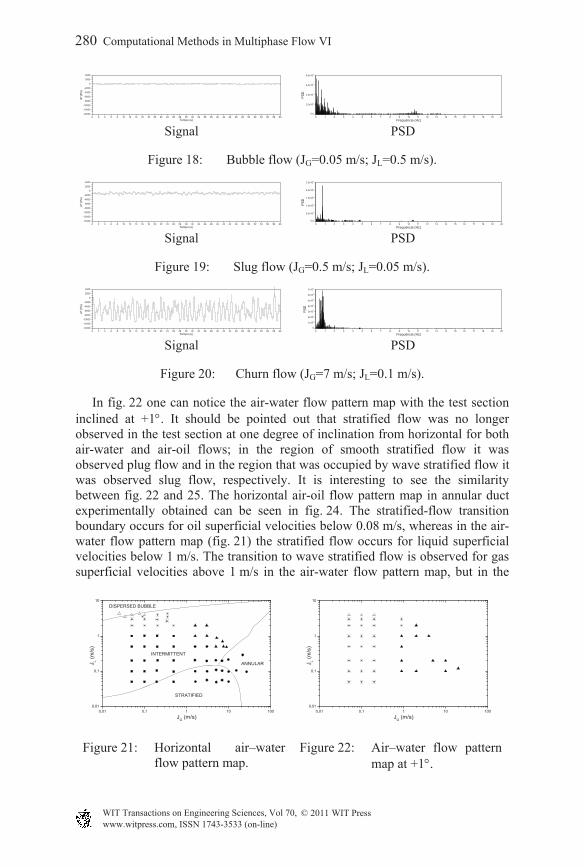
3.2.2 Inclined flow (45) Figs. 18-20 illustrate the time-domain signals in upward inclined air-water bubble, slug and churn flow, respectively. The pressure signature related to bubble flow is smoother than that of slug or churn flow. In addition, the PSD indicates the presence of high frequency oscillations around 10 Hz only for bubble flow. In churn flow, fig. 20, the signal is characterized by high amplitude. It is worth noting that the signal related to churn flow can reach values that overcome the value of the hydrostatic pressure of water (10.4 kPa). This feature of the signal obtained in churn flow is likely due to a frictional pressure loss of downward liquid film flow added with the high void fraction.

3.3 Flow patterns maps

In modeling horizontal annular duct, Blanco et. al. [8] chose to use a model proposed by Rodriguez et al. [9] to define the stratified-flow transition boundaries and the approach proposed by Taitel and Dukler [10] to define all the other transitions. Fig. 20 illustrates the horizontal air-water flow pattern map drawn by Blanco et al. [8] and the flow pattern map obtained experimentally in this work. Some inconsistency can be observed when comparing data with predictions. The flow map of Blanco et al. [8] predicts the transition from stratified to intermittent flow for liquid superficial velocities below 0.2 m/s, but according to the data such transition occurs at liquid superficial velocity around 1 m/s. The stratified wavy flow was observed up to gas superficial velocity of 20 m/s in the experiments, whereas the flow map proposed by Blanco et al. [8] predicts annular flow.

0 2 4 6 8 10 12 14 16 18 20 22 24 26 28 30 32 34 36 38 40 42 44 46 48 50 52 54 56 58 60

0

1000

2000

3000

4000

5000

6000

7000

8000P

(P

a)

Tempo (s)0 1 2 3 4 5 6 7 8 9 10 11 12 13 14 15 16 17 18 19 20

0

1x104

2x104

3x104

4x104

5x104

6x104

PS

D

Frequência (Hz)

0 2 4 6 8 10 12 14 16 18 20 22 24 26 28 30 32 34 36 38 40 42 44 46 48 50 52 54 56 58 600

1000

2000

3000

4000

5000

6000

7000

8000

P (

Pa)

Tempo (s)0 1 2 3 4 5 6 7 8 9 10 11 12 13 14 15 16 17 18 19 20

0,0

2,0x103

4,0x103

6,0x103

8,0x103

1,0x104

PS

D

Frequência (Hz)



33

Signal

PSD

Figure 18: Bubble flow (JG=0.05 m/s; JL=0.5 m/s).

Signal

PSD

Figure 19: Slug flow (JG=0.5 m/s; JL=0.05 m/s).

Signal

PSD

Figure 20: Churn flow (JG=7 m/s; JL=0.1 m/s).

In fig. 22 one can notice the air-water flow pattern map with the test section inclined at +1. It should be pointed out that stratified flow was no longer observed in the test section at one degree of inclination from horizontal for both air-water and air-oil flows; in the region of smooth stratified flow it was observed plug flow and in the region that was occupied by wave stratified flow it was observed slug flow, respectively. It is interesting to see the similarity between fig. 22 and 25. The horizontal air-oil flow pattern map in annular duct experimentally obtained can be seen in fig. 24. The stratified-flow transition boundary occurs for oil superficial velocities below 0.08 m/s, whereas in the air-water flow pattern map (fig. 21) the stratified flow occurs for liquid superficial velocities below 1 m/s. The transition to wave stratified flow is observed for gas superficial velocities above 1 m/s in the air-water flow pattern map, but in the

Figure 21: Horizontal air–water flow pattern map.

Figure 22: Air–water flow pattern map at +1.

0 2 4 6 8 10 12 14 16 18 20 22 24 26 28 30 32 34 36 38 40 42 44 46 48 50 52 54 56 58 60-14000

-12000

-10000

-8000

-6000

-4000

-2000

0

2000

4000

P (

Pa)

Tempo (s)0 1 2 3 4 5 6 7 8 9 10 11 12 13 14 15 16 17 18 19 20

0,0

2,0x101

4,0x101

6,0x101

8,0x101

PS

D

Frequência (Hz)

0 2 4 6 8 10 12 14 16 18 20 22 24 26 28 30 32 34 36 38 40 42 44 46 48 50 52 54 56 58 60-14000

-12000

-10000

-8000

-6000

-4000

-2000

0

2000

4000

P (

Pa)

Tempo (s)0 1 2 3 4 5 6 7 8 9 10 11 12 13 14 15 16 17 18 19 20

0,0

5,0x103

1,0x104

1,5x104

2,0x104

2,5x104

PS

D

Frequência (Hz)

0 2 4 6 8 10 12 14 16 18 20 22 24 26 28 30 32 34 36 38 40 42 44 46 48 50 52 54 56 58 60-14000

-12000

-10000

-8000

-6000

-4000

-2000

0

2000

4000

P (

Pa)

Tempo (s)0 1 2 3 4 5 6 7 8 9 10 11 12 13 14 15 16 17 18 19 20

0

1x105

2x105

3x105

4x105

5x105

6x105

7x105

PS

D

Frequência (Hz)

0,01 0,1 1 10 1000,01

0,1

1

10

J L (m

/s)

JG (m/s)

STRATIFIED

ANNULAR

INTERMITTENT

DISPERSED BUBBLE

0,01 0,1 1 10 1000,01

0,1

1

10

J L (m

/s)

JG (m/s)



33

case of air-oil the boundary transition from smooth stratified flow to wave stratified flow occurs for gas superficial velocities above 0.1 m/s. The slug flow is observed at gas superficial velocities above 0.5 m/s in both air-oil and air-water flows. As one can see in fig. 23, the methodology proposed by Blanco et al. [8] for upward gas-liquid annular duct flow at several inclinations was able to predict with quite good accuracy the various observed flow patterns. The flow patterns bubble, slug, churn and dispersed bubble were observed with the test section inclined at 45. The plug flow observed in the air-water flow pattern map at one degree of inclination from horizontal was not observed in the air-water flow pattern map at +45. The dispersed bubble flow occurs for liquid superficial velocities above 4 m/s for the flow pattern map at +1 and liquid superficial velocities above 2 m/s for the flow pattern map at +45.

Figure 23: Air–water flow pattern map at +45.

Figure 24: Horizontal air–oil flow pattern map.

Figure 25: Air–oil flow pattern

map at +1.

4 Conclusion

Air-water and air-oil flow patterns for horizontal and inclined flow in a large annular duct were identified and characterized in this study. The experimental results were obtained in a 10.5 m length test section of borosilicate glass with inner diameter of 75 mm and outer diameter of 111 mm. The inclinations of the

0,01 0,1 1 10 1000,01

0,1

1

10

J L (m

/s)

JG (m/s)

CHURNSLUGBUBBLE ANNULAR

DISPERSED BUBBLE

0,01 0,1 1 10 100

0,01

0,1

1

J L (m

/s)

JG (m/s)

0,01 0,1 1 10 1000,01

0,1

1

J L (m

/s)

JG (m/s)

STRATIFIED SMOOTH STRATIFIED WAVY PLUG SLUG CHURN BUBBLE DISPERSED BUBBLE



33

test section were 0, +1 and +45 in relation to horizontal. The ranges of superficial velocities of water, oil and air were 0,044 to 4,373 m/s, 0,01 to 0,5 m/s and 0,025 to 26,78 m/s, respectively. The flow patterns smooth stratified, wavy stratified, intermittent (plug and slug) and dispersed bubbles were identified at zero degrees of inclination (horizontal). With the test section inclined at one degree, bubbles, intermittent and dispersed bubbles were identified. In the tests where the test section was inclined at 45, bubbles, slug, churn and dispersed bubbles were observed. The transition to wave stratified flow is observed for gas superficial velocities above 1 m/s in the air-water flow pattern map, but in the case of air-oil the boundary transition from smooth stratified flow to wave stratified flow occurs for gas superficial velocities above 0.1 m/s. The slug flow is observed at gas superficial velocities above 0.5 m/s in both air-oil and air-water flows. The plug flow observed in the air-water flow pattern map at one degree of inclination from horizontal was not observed in the air-water flow pattern map at +45. The dispersed bubble flow occurs for liquid superficial velocities above 4 m/s for the flow pattern map at +1 and liquid superficial velocities above 2 m/s for the flow pattern map at +45. The results of this study help to assess the potentiality of using a simple pressure-signature objective technique as a tool in identifying flow pattern transition boundaries in air-water and air-oil flows in a big annular duct. Another finding is the clear necessity of developing a phenomenological model capable of accurately generate flow pattern maps for horizontal gas-liquid flow in annular duct with dimensions similar to that used in the petroleum industry.

Acknowledgement

The present study was financially supported by PETROBRAS, whose guidance and assistance are gratefully acknowledged.

References

[1] Kelessidis, V.C. and Dukler, A.E., Modeling flow pattern transitions for upward gas-liquid flow in vertical concentric end eccentric annuli, International Journal of Multiphase Flow, 15(2), pp. 173-191, 1989.

[2] Hasan, A.R. and Kabir, C.S., Two-phase flow in vertical and inclined annuli, International Journal of Multiphase Flow, 18(2), pp. 279-293, 1992.

[3] Caetano, E.F., Shoham, O. and Brill, J.P., Upward vertical two-phase flow through an annulus. Part I: Single-phase fiction factor, Taylor bubbles rise velocity and flow pattern prediction, Journal of Energy Resources Technology, 114, pp. 1-13, 1992.

[4] Wongwises, S. and Pipathattakul, M., Flow pattern, pressure drop and void fraction of two-phase gas-liquid flow in an inclined narrow annular channel. Experimental Thermal and Fluid Science, 30(4), pp. 345-354, 2006.



33

[5] Ekberg, N.P., Ghiaasiaan, S.M., Abdel-Khalik, S.I., Yoda, M. and Jeter, S.M., Gas-liquid two-phase flow in narrow horizontal annuli, Nuclear Engineering and Design, 192(1), pp. 59-80, 1999.

[6] J. Drahos, J. Cermak and K. Selucky, Characterization of Hydrodynamic Regimes in Horizontal Two-Phase Flow Part II: Analysis of Wall Pressure Fluctuations, Chem. Eng. Process., vol. 22, pp. 45-52, 1987.

[7] G. Matsui, Automatic identification of flow regimes in vertical two-phase flow using differential pressure fluctuations, Nuclear Engineering and Design, vol. 95, pp. 221-231, 1986.

[8] Blanco C.P., Albieri T.F. and Rodriguez O.M.H., Revisão de modelos para transição de padrão de escoamento gás-líquido em duto anular vertical e horizontal, ENCIT 2008, Belo Horizonte, Brazil, 2008.

[9] Rodriguez, O.M.H.; Mudde, R.F.; Oliemans, R.V.A., Stability analysis of slightly-inclined stratified oil-water flow, including the distribution coefficients and the cross-section curvature. In: North American Conference on Multiphase Technology, 5, 2006, Banff, Canada. Proceedings. Banff, Canada: BHR Group Limited. p.229-245.

[10] Taitel, Y. and Dukler, A. E., A model for predicting flow regime transitions in horizontal and near horizontal gas-liquid flow, A.I.Ch.E. Journal, 22, pp. 47-55, 1976.



33

flow patterns in inclined gas-liquid annular duct flow · flow patterns in inclined gas-liquid...

Documents