fluid mechanic ll (chapter 3)
DESCRIPTION
nota dari buku fluid mechanic...harap ini dapat membantu pada sesiapa yang nak beli buku tp kurang mampu tu...boleh rujuk siniTRANSCRIPT
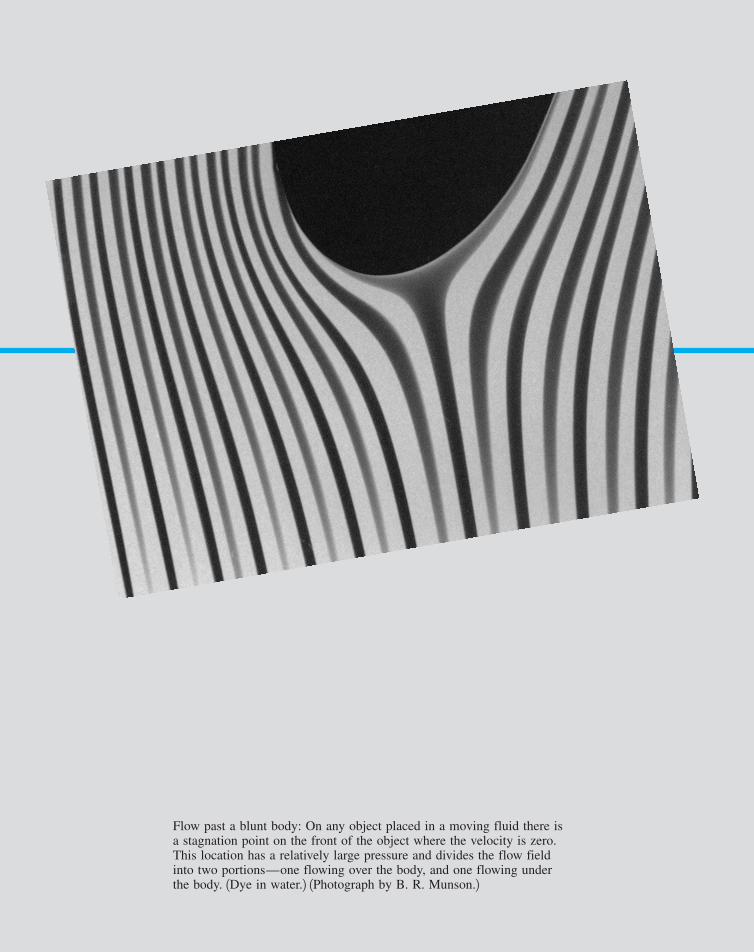
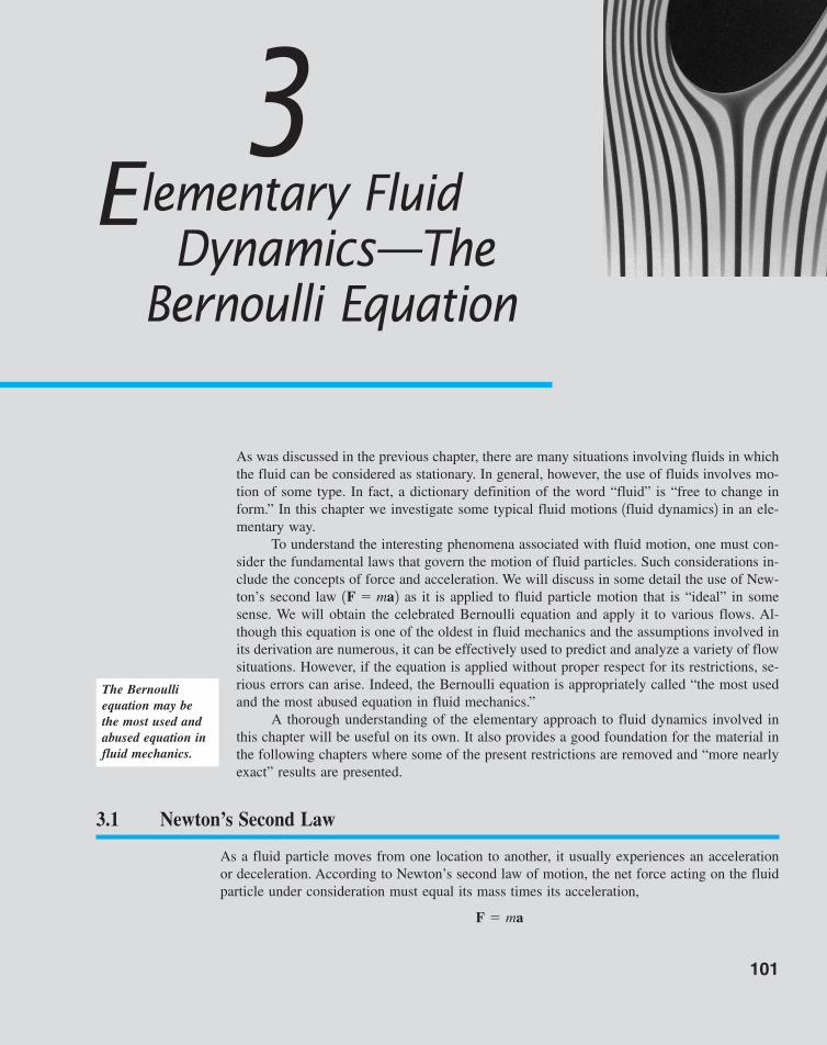
Flow past a blunt body: On any object placed in a moving fluid there isa stagnation point on the front of the object where the velocity is zero.This location has a relatively large pressure and divides the flow fieldinto two portions—one flowing over the body, and one flowing underthe body. 1Dye in water.2 1Photograph by B. R. Munson.2
7708d_c03_100 8/10/01 3:01 PM Page 100 mac120 mac120:1st shift:
As was discussed in the previous chapter, there are many situations involving fluids in whichthe fluid can be considered as stationary. In general, however, the use of fluids involves mo-tion of some type. In fact, a dictionary definition of the word “fluid” is “free to change inform.” In this chapter we investigate some typical fluid motions 1fluid dynamics2 in an ele-mentary way.
To understand the interesting phenomena associated with fluid motion, one must con-sider the fundamental laws that govern the motion of fluid particles. Such considerations in-clude the concepts of force and acceleration. We will discuss in some detail the use of New-ton’s second law as it is applied to fluid particle motion that is “ideal” in somesense. We will obtain the celebrated Bernoulli equation and apply it to various flows. Al-though this equation is one of the oldest in fluid mechanics and the assumptions involved inits derivation are numerous, it can be effectively used to predict and analyze a variety of flowsituations. However, if the equation is applied without proper respect for its restrictions, se-rious errors can arise. Indeed, the Bernoulli equation is appropriately called “the most usedand the most abused equation in fluid mechanics.”
A thorough understanding of the elementary approach to fluid dynamics involved inthis chapter will be useful on its own. It also provides a good foundation for the material inthe following chapters where some of the present restrictions are removed and “more nearlyexact” results are presented.
1F � ma2
101
3Elementary Fluid
Dynamics—TheBernoulli Equation
3.1 Newton’s Second Law
As a fluid particle moves from one location to another, it usually experiences an accelerationor deceleration. According to Newton’s second law of motion, the net force acting on the fluidparticle under consideration must equal its mass times its acceleration,
F � ma
The Bernoulliequation may bethe most used andabused equation influid mechanics.
7708d_c03_101 8/10/01 3:01 PM Page 101 mac120 mac120:1st shift:
In this chapter we consider the motion of inviscid fluids. That is, the fluid is assumed to havezero viscosity. If the viscosity is zero, then the thermal conductivity of the fluid is also zeroand there can be no heat transfer 1except by radiation2.
In practice there are no inviscid fluids, since every fluid supports shear stresses whenit is subjected to a rate of strain displacement. For many flow situations the viscous effectsare relatively small compared with other effects. As a first approximation for such cases itis often possible to ignore viscous effects. For example, often the viscous forces developedin flowing water may be several orders of magnitude smaller than forces due to other influ-ences, such as gravity or pressure differences. For other water flow situations, however, theviscous effects may be the dominant ones. Similarly, the viscous effects associated with theflow of a gas are often negligible, although in some circumstances they are very important.
We assume that the fluid motion is governed by pressure and gravity forces only andexamine Newton’s second law as it applies to a fluid particle in the form:
The results of the interaction between the pressure, gravity, and acceleration provide nu-merous useful applications in fluid mechanics.
To apply Newton’s second law to a fluid 1or any other object2, we must define an ap-propriate coordinate system in which to describe the motion. In general the motion will bethree-dimensional and unsteady so that three space coordinates and time are needed to de-scribe it. There are numerous coordinate systems available, including the most often usedrectangular and cylindrical systems. Usually the specific flow geometry dic-tates which system would be most appropriate.
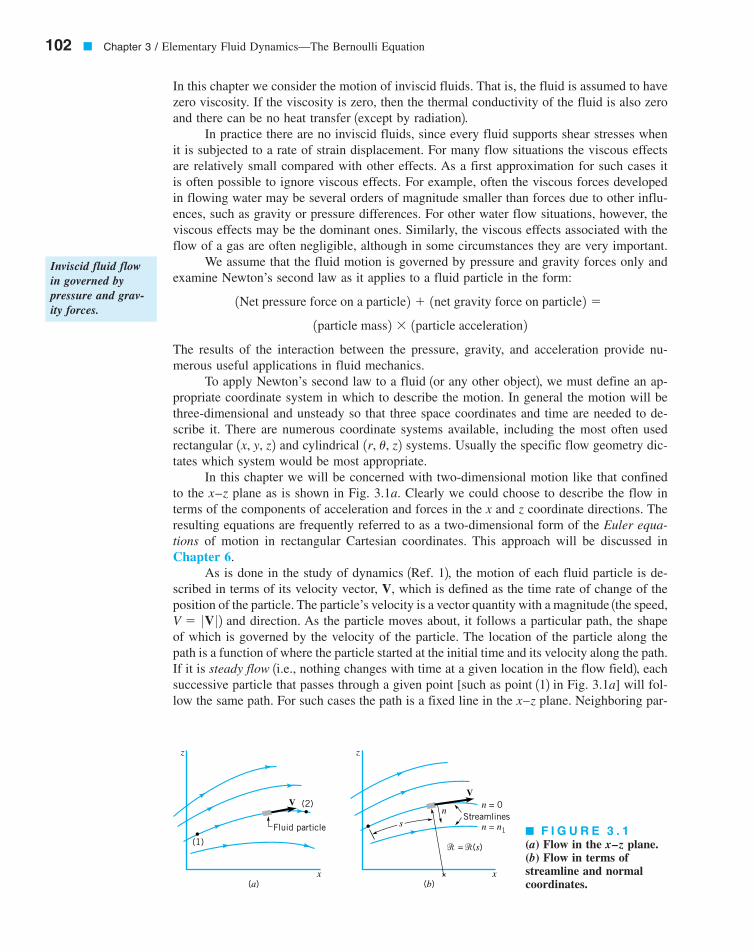
In this chapter we will be concerned with two-dimensional motion like that confinedto the x–z plane as is shown in Fig. 3.1a. Clearly we could choose to describe the flow interms of the components of acceleration and forces in the x and z coordinate directions. Theresulting equations are frequently referred to as a two-dimensional form of the Euler equa-tions of motion in rectangular Cartesian coordinates. This approach will be discussed inChapter 6.
As is done in the study of dynamics 1Ref. 12, the motion of each fluid particle is de-scribed in terms of its velocity vector, V, which is defined as the time rate of change of theposition of the particle. The particle’s velocity is a vector quantity with a magnitude 1the speed,
2 and direction. As the particle moves about, it follows a particular path, the shapeof which is governed by the velocity of the particle. The location of the particle along thepath is a function of where the particle started at the initial time and its velocity along the path.If it is steady flow 1i.e., nothing changes with time at a given location in the flow field2, eachsuccessive particle that passes through a given point [such as point 112 in Fig. 3.1a] will fol-low the same path. For such cases the path is a fixed line in the x–z plane. Neighboring par-
V � 0V 0
1r, u, z21x, y, z2
1particle mass2 � 1particle acceleration2
1Net pressure force on a particle2 � 1net gravity force on particle2 �
102 � Chapter 3 / Elementary Fluid Dynamics—The Bernoulli Equation
z
x
Fluid particle
(1)
(2)V
z
x
Streamlinesn = 0
n = n1
n
V
s
= (s)
(a) (b)
� �
� F I G U R E 3 . 1(a) Flow in the x–z plane.(b) Flow in terms ofstreamline and normal coordinates.
Inviscid fluid flowin governed bypressure and grav-ity forces.
7708d_c03_102 8/10/01 3:02 PM Page 102 mac120 mac120:1st shift:
ticles that pass on either side of point 112 follow their own paths, which may be of a differ-ent shape than the one passing through 112. The entire x–z plane is filled with such paths.
For steady flows each particle slides along its path, and its velocity vector is every-where tangent to the path. The lines that are tangent to the velocity vectors throughout theflow field are called streamlines. For many situations it is easiest to describe the flow in termsof the “streamline” coordinates based on the streamlines as are illustrated in Fig. 3.1b. Theparticle motion is described in terms of its distance, along the streamline from someconvenient origin and the local radius of curvature of the streamline, The dis-tance along the streamline is related to the particle’s speed by and the radius ofcurvature is related to shape of the streamline. In addition to the coordinate along the stream-line, s, the coordinate normal to the streamline, n, as is shown in Fig. 3.1b, will be of use.
To apply Newton’s second law to a particle flowing along its streamline, we must writethe particle acceleration in terms of the streamline coordinates. By definition, the accelera-tion is the time rate of change of the velocity of the particle, For two-dimensionalflow in the x–z plane, the acceleration has two components—one along the streamline,the streamwise acceleration, and one normal to the streamline, the normal acceleration.
The streamwise acceleration results from the fact that the speed of the particle gener-ally varies along the streamline, For example, in Fig. 3.1a the speed may be at point 112 and at point 122. Thus, by use of the chain rule of differentiation, the scomponent of the acceleration is given by We haveused the fact that The normal component of acceleration, the centrifugal accel-eration, is given in terms of the particle speed and the radius of curvature of its path. Thus,
where both V and may vary along the streamline. These equations for the ac-celeration should be familiar from the study of particle motion in physics 1Ref. 22 or dy-namics 1Ref. 12. A more complete derivation and discussion of these topics can be found inChapter 4.
Thus, the components of acceleration in the s and n directions, and are given by
(3.1)
where is the local radius of curvature of the streamline, and s is the distance measuredalong the streamline from some arbitrary initial point. In general there is acceleration alongthe streamline 1because the particle speed changes along its path, 2 and accelerationnormal to the streamline 1because the particle does not flow in a straight line, 2. Toproduce this acceleration there must be a net, nonzero force on the fluid particle.
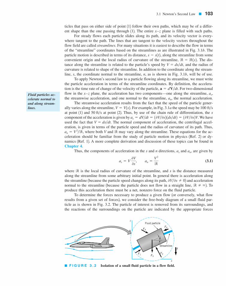
To determine the forces necessary to produce a given flow 1or conversely, what flowresults from a given set of forces2, we consider the free-body diagram of a small fluid par-ticle as is shown in Fig. 3.2. The particle of interest is removed from its surroundings, andthe reactions of the surroundings on the particle are indicated by the appropriate forces
r � �0V�0s � 0
r
as � V 0V
0s, an �
V 2
r
an,as
ran � V 2�r,
V � ds�dt.as � dV�dt � 10V�0s2 1ds�dt2 � 10V�0s2V.
50 ft�s100 ft�sV � V1s2.
an,as,
a � dV�dt.
V � ds�dt,r � r1s2.
s � s1t2,
3.1 Newton’s Second Law � 103
Fluid particles ac-celerate normal toand along stream-lines.
� F I G U R E 3 . 2 Isolation of a small fluid particle in a flow field.
F1F2F3
F4F5
θ
Streamline
Fluid particle
g
x
z
7708d_c03_103 8/10/01 3:03 PM Page 103 mac120 mac120:1st shift:
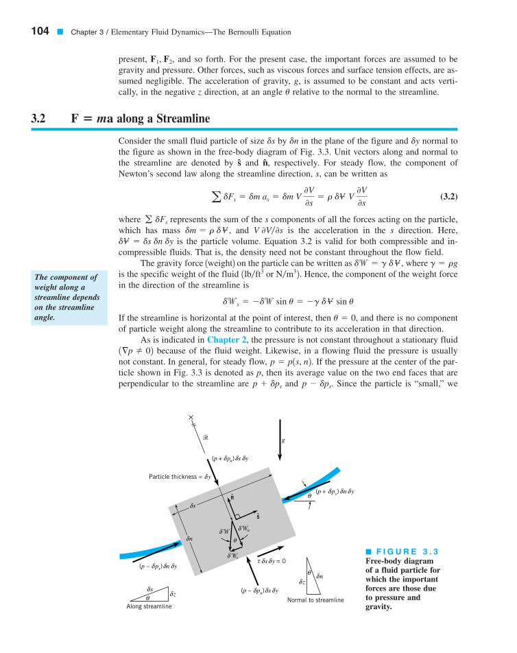
present, and so forth. For the present case, the important forces are assumed to begravity and pressure. Other forces, such as viscous forces and surface tension effects, are as-sumed negligible. The acceleration of gravity, g, is assumed to be constant and acts verti-cally, in the negative z direction, at an angle relative to the normal to the streamline.u
F1, F2,
104 � Chapter 3 / Elementary Fluid Dynamics—The Bernoulli Equation
3.2 along a StreamlineF � ma
Consider the small fluid particle of size by in the plane of the figure and normal tothe figure as shown in the free-body diagram of Fig. 3.3. Unit vectors along and normal tothe streamline are denoted by and respectively. For steady flow, the component ofNewton’s second law along the streamline direction, s, can be written as
(3.2)
where represents the sum of the s components of all the forces acting on the particle,which has mass and is the acceleration in the s direction. Here,
is the particle volume. Equation 3.2 is valid for both compressible and in-compressible fluids. That is, the density need not be constant throughout the flow field.
The gravity force 1weight2 on the particle can be written as where is the specific weight of the fluid Hence, the component of the weight forcein the direction of the streamline is
If the streamline is horizontal at the point of interest, then and there is no componentof particle weight along the streamline to contribute to its acceleration in that direction.
As is indicated in Chapter 2, the pressure is not constant throughout a stationary fluidbecause of the fluid weight. Likewise, in a flowing fluid the pressure is usually
not constant. In general, for steady flow, If the pressure at the center of the par-ticle shown in Fig. 3.3 is denoted as p, then its average value on the two end faces that areperpendicular to the streamline are and Since the particle is “small,” wep � dps.p � dps
p � p1s, n2.1§p � 02
u � 0,
dws � �dw sin u � �g dV� sin u
1lb�ft3 or N�m32.g � rgdw � g dV�,
dV� � ds dn dyV 0V�0sdm � r dV�,
g dFs
a dFs � dm as � dm V 0V
0s� r dV� V
0V
0s
n,s
dydnds
� F I G U R E 3 . 3Free-body diagramof a fluid particle forwhich the importantforces are those dueto pressure and gravity.
Particle thickness = y
Along streamlineNormal to streamline
g�
(p + pn) s yδ δ δ
δ
(p + ps) n yδ δ δ
(p – ps) n yδ δ δ
(p – pn) s yδ δ δ
s yδ δτ = 0
sδ zδθ
zδθ
nδ
sδ
nδ
s
nδδ
sδ
θ
θn
��
�
The component ofweight along astreamline dependson the streamlineangle.
7708d_c03_104 8/10/01 3:04 PM Page 104 mac120 mac120:1st shift:
can use a one-term Taylor series expansion for the pressure field 1as was done in Chapter 2for the pressure forces in static fluids2 to obtain
Thus, if is the net pressure force on the particle in the streamline direction, it followsthat
Note that the actual level of the pressure, p, is not important. What produces a net pres-sure force is the fact that the pressure is not constant throughout the fluid. The nonzero pres-sure gradient, is what provides a net pressure force on the parti-cle. Viscous forces, represented by are zero, since the fluid is inviscid.
Thus, the net force acting in the streamline direction on the particle shown in Fig. 3.3is given by
(3.3)
By combining Eqs. 3.2 and 3.3, we obtain the following equation of motion along the stream-line direction:
(3.4)
We have divided out the common particle volume factor, that appears in both the forceand the acceleration portions of the equation. This is a representation of the fact that it is thefluid density 1mass per unit volume2, not the mass, per se, of the fluid particle that is important.
The physical interpretation of Eq. 3.4 is that a change in fluid particle speed is ac-complished by the appropriate combination of pressure gradient and particle weight alongthe streamline. For fluid static situations this balance between pressure and gravity forces issuch that no change in particle speed is produced—the right-hand side of Eq. 3.4 is zero,and the particle remains stationary. In a flowing fluid the pressure and weight forces do notnecessarily balance—the force unbalance provides the appropriate acceleration and, hence,particle motion.
dV�,
�g sin u �0p
0s� rV
0V
0s� ras
a dFs � dws � dFps � a�g sin u �0p
0sb dV�
t ds dy,§p � 0p�0s s � 0p�0n n,
� �0p
0s ds dn dy � �
0p
0s dV�
dFps � 1p � dps2 dn dy � 1p � dps2 dn dy � �2 dps dn dy
dFps
dps �0p
0s ds
2
3.2 F � ma along a Streamline � 105
EXAMPLE3.1
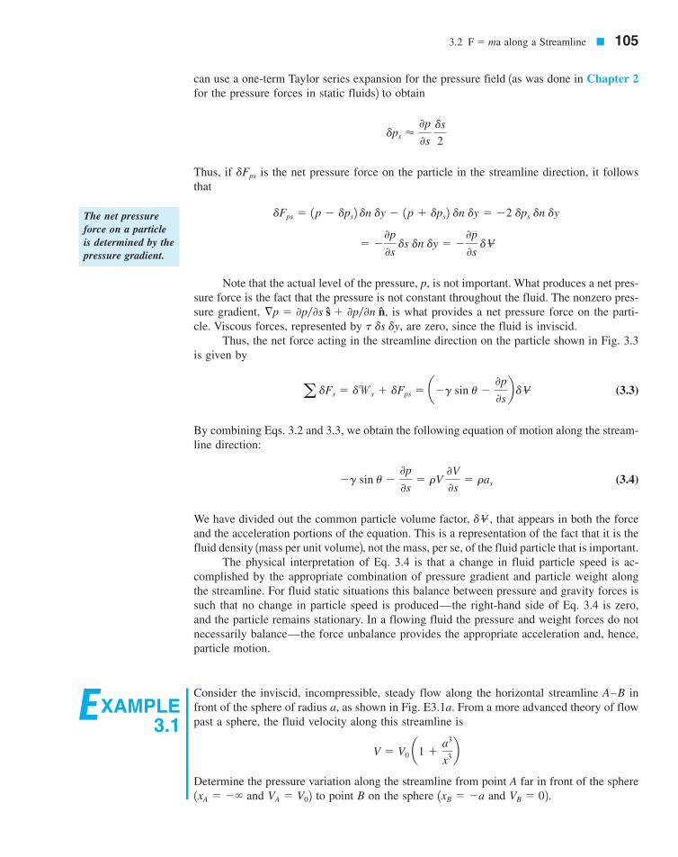
Consider the inviscid, incompressible, steady flow along the horizontal streamline A–B infront of the sphere of radius a, as shown in Fig. E3.1a. From a more advanced theory of flowpast a sphere, the fluid velocity along this streamline is
Determine the pressure variation along the streamline from point A far in front of the sphereand to point B on the sphere and VB � 02.1xB � �aVA � V021xA � ��
V � V0 a1 �a3
x3b
The net pressureforce on a particleis determined by thepressure gradient.
7708d_c03_105 8/10/01 3:05 PM Page 105 mac120 mac120:1st shift:
106 � Chapter 3 / Elementary Fluid Dynamics—The Bernoulli Equation
SOLUTION
Since the flow is steady and inviscid, Eq. 3.4 is valid. In addition, since the streamline ishorizontal, and the equation of motion along the streamline reduces to
(1)
With the given velocity variation along the streamline, the acceleration term is
where we have replaced s by x since the two coordinates are identical 1within an additiveconstant2 along streamline A–B. It follows that along the streamline. The fluidslows down from far ahead of the sphere to zero velocity on the “nose” of the sphere
Thus, according to Eq. 1, to produce the given motion the pressure gradient along thestreamline is
(2)
This variation is indicated in Fig. E3.1b. It is seen that the pressure increases in the direc-tion of flow from point A to point B. The maximum pressure gradient
occurs just slightly ahead of the sphere It is the pressure gra-dient that slows the fluid down from to
The pressure distribution along the streamline can be obtained by integrating Eq. 2from 1gage2 at to pressure p at location x. The result, plotted in Fig. E3.1c,is
(Ans)p � �rV 02 c aa
xb3
�1a�x26
2d
x � ��p � 0
VB � 0.VA � V0
1x � �1.205a2.10.610 rV 20 �a210p�0x 7 02
0p
0x�
3ra3V 02 11 � a3�x32
x4
1x � �a2. V0
V 0V�0s 6 0
V 0V
0s� V
0V
0x� V0 a1 �
a3
x3b a�3V0a3
x4 b � �3V 02 a1 �
a3
x3b a3
x4
0p
0s� �rV
0V
0s
sin u � sin 0° � 0
VA = VO i
A
V = V i VB = 0B
a
z
(a)
x
–3a –2a –a 0 x
∂p__∂x
0.610 V02/aρ
(b)–3a –2a –a 0 x
(c)
p
0.5 V02ρ
^ ^
� F I G U R E E 3 . 1
7708d_c03_106 8/10/01 3:05 PM Page 106 mac120 mac120:1st shift:
3.2 F � ma along a Streamline � 107
The pressure at B, a stagnation point since is the highest pressure along the stream-line As shown in Chapter 9, this excess pressure on the front of the sphere1i.e., 2 contributes to the net drag force on the sphere. Note that the pressure gradientand pressure are directly proportional to the density of the fluid, a representation of the factthat the fluid inertia is proportional to its mass.
pB 7 01pB � rV 2
0 �22.VB � 0,
Equation 3.4 can be rearranged and integrated as follows. First, we note from Fig. 3.3that along the streamline Also, we can write Finally,along the streamline the value of n is constant so that
Hence, along the streamline These ideas combinedwith Eq. 3.4 give the following result valid along a streamline
This simplifies to
(3.5)
which can be integrated to give
(3.6)
where C is a constant of integration to be determined by the conditions at some point on thestreamline.
In general it is not possible to integrate the pressure term because the density may notbe constant and, therefore, cannot be removed from under the integral sign. To carry out thisintegration we must know specifically how the density varies with pressure. This is not al-ways easily determined. For example, for a perfect gas the density, pressure, and tempera-ture are related according to where R is the gas constant. To know how the den-sity varies with pressure, we must also know the temperature variation. For now we willassume that the density is constant 1incompressible flow2. The justification for this assump-tion and the consequences of compressibility will be considered further in Section 3.8.1 andmore fully in Chapter 11.
With the additional assumption that the density remains constant 1a very good as-sumption for liquids and also for gases if the speed is “not too high”2, Eq. 3.6 assumes thefollowing simple representation for steady, inviscid, incompressible flow.
(3.7)
This is the celebrated Bernoulli equation—a very powerful tool in fluid mechanics. In 1738Daniel Bernoulli 11700–17822 published his Hydrodynamics in which an equivalent of thisfamous equation first appeared. To use it correctly we must constantly remember the basicassumptions used in its derivation: 112 viscous effects are assumed negligible, 122 the flow isassumed to be steady, 132 the flow is assumed to be incompressible, 142 the equation is ap-plicable along a streamline. In the derivation of Eq. 3.7, we assume that the flow takes placein a plane 1the x–z plane2. In general, this equation is valid for both planar and nonplanar1three-dimensional2 flows, provided it is applied along the streamline.
p � 12rV
2 � gz � constant along streamline
p � rRT,
� dpr
�1
2 V 2 � gz � C 1along a streamline2
dp �1
2 rd1V 22 � g dz � 0 1along a streamline2
�g dz
ds�
dp
ds�
1
2 r
d1V 22
ds
0p�0s � dp�ds.10p�0n2 dn � 10p�0s2 ds.dp � 10p�0s2 ds �1dn � 02
V dV�ds � 12d1V
22�ds.sin u � dz�ds.
The Bernoulliequation can be ob-tained by integrat-ing along astreamline.
F � ma
V3.1 Balancing ball
7708d_c03_107 8/10/01 3:06 PM Page 107 mac120 mac120:1st shift:
We will provide many examples to illustrate the correct use of the Bernoulli equationand will show how a violation of the basic assumptions used in the derivation of this equa-tion can lead to erroneous conclusions. The constant of integration in the Bernoulli equationcan be evaluated if sufficient information about the flow is known at one location along thestreamline.
108 � Chapter 3 / Elementary Fluid Dynamics—The Bernoulli Equation
The difference in fluid velocity between two point in a flow field, and can oftenbe controlled by appropriate geometric constraints of the fluid. For example, a garden hosenozzle is designed to give a much higher velocity at the exit of the nozzle than at its entrancewhere it is attached to the hose. As is shown by the Bernoulli equation, the pressure within
V2,V1
EXAMPLE3.2
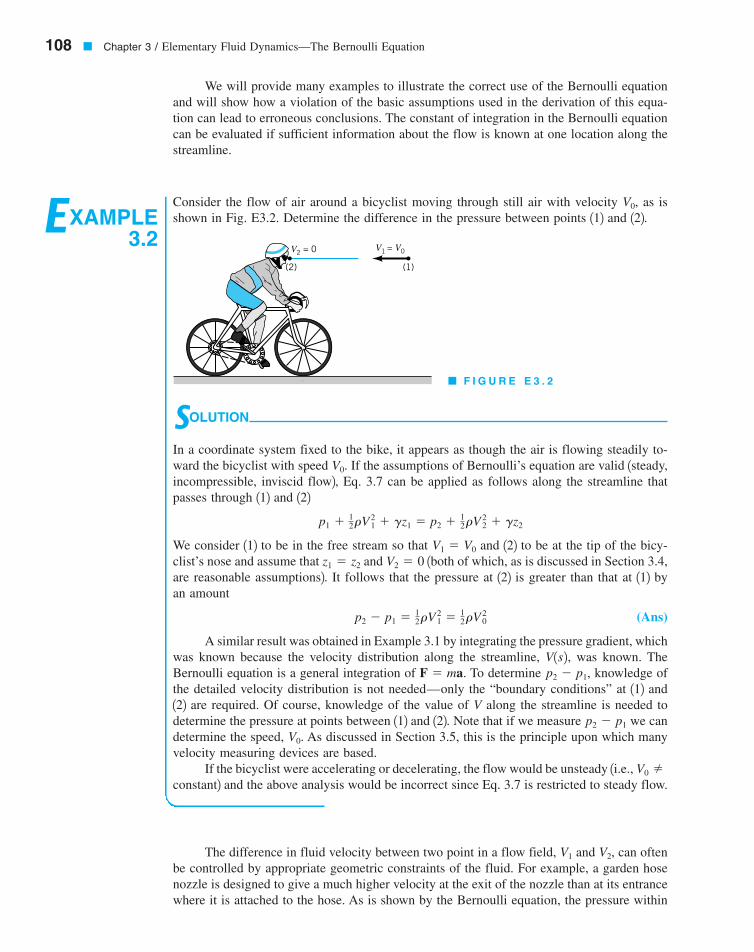
Consider the flow of air around a bicyclist moving through still air with velocity as isshown in Fig. E3.2. Determine the difference in the pressure between points 112 and 122.
V0,
SOLUTION
In a coordinate system fixed to the bike, it appears as though the air is flowing steadily to-ward the bicyclist with speed If the assumptions of Bernoulli’s equation are valid 1steady,incompressible, inviscid flow2, Eq. 3.7 can be applied as follows along the streamline thatpasses through 112 and 122
We consider 112 to be in the free stream so that and 122 to be at the tip of the bicy-clist’s nose and assume that and 1both of which, as is discussed in Section 3.4,are reasonable assumptions2. It follows that the pressure at 122 is greater than that at 112 byan amount
(Ans)
A similar result was obtained in Example 3.1 by integrating the pressure gradient, whichwas known because the velocity distribution along the streamline, was known. TheBernoulli equation is a general integration of To determine knowledge ofthe detailed velocity distribution is not needed—only the “boundary conditions” at 112 and122 are required. Of course, knowledge of the value of V along the streamline is needed todetermine the pressure at points between 112 and 122. Note that if we measure we candetermine the speed, As discussed in Section 3.5, this is the principle upon which manyvelocity measuring devices are based.
If the bicyclist were accelerating or decelerating, the flow would be unsteady 1i.e.,constant2 and the above analysis would be incorrect since Eq. 3.7 is restricted to steady flow.
V0 �
V0.p2 � p1
p2 � p1,F � ma.V1s2,
p2 � p1 � 12rV 1
2 � 12rV 0
2
V2 � 0z1 � z2
V1 � V0
p1 � 12rV 1
2 � gz1 � p2 � 12rV 2
2 � gz2
V0.
V2 = 0 V1 = V0
(1)(2)
� F I G U R E E 3 . 2
7708d_c03_108 8/10/01 3:12 PM Page 108 mac120 mac120:1st shift:
the hose must be larger than that at the exit 1for constant elevation, an increase in velocityrequires a decrease in pressure if Eq. 3.7 is valid2. It is this pressure drop that accelerates thewater through the nozzle. Similarly, an airfoil is designed so that the fluid velocity over itsupper surface is greater 1on the average2 than that along its lower surface. From the Bernoulliequation, therefore, the average pressure on the lower surface is greater than that on the up-per surface. A net upward force, the lift, results.
3.3 F � ma Normal to a Streamline � 109
3.3 Normal to a StreamlineF � ma
In this section we will consider application of Newton’s second law in a direction normal tothe streamline. In many flows the streamlines are relatively straight, the flow is essentiallyone-dimensional, and variations in parameters across streamlines 1in the normal direction2can often be neglected when compared to the variations along the streamline. However, innumerous other situations valuable information can be obtained from considering normal to the streamlines. For example, the devastating low-pressure region at the center ofa tornado can be explained by applying Newton’s second law across the nearly circular stream-lines of the tornado.
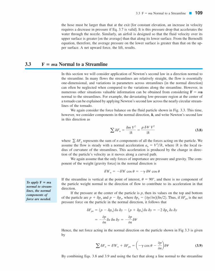
We again consider the force balance on the fluid particle shown in Fig. 3.3. This time,however, we consider components in the normal direction, and write Newton’s second lawin this direction as
(3.8)
where represents the sum of n components of all the forces acting on the particle. Weassume the flow is steady with a normal acceleration where is the local ra-dius of curvature of the streamlines. This acceleration is produced by the change in direc-tion of the particle’s velocity as it moves along a curved path.
We again assume that the only forces of importance are pressure and gravity. The com-ponent of the weight 1gravity force2 in the normal direction is
If the streamline is vertical at the point of interest, and there is no component ofthe particle weight normal to the direction of flow to contribute to its acceleration in thatdirection.
If the pressure at the center of the particle is p, then its values on the top and bottomof the particle are and where Thus, if is the netpressure force on the particle in the normal direction, it follows that
Hence, the net force acting in the normal direction on the particle shown in Fig 3.3 is givenby
(3.9)
By combining Eqs. 3.8 and 3.9 and using the fact that along a line normal to the streamline
a dFn � dwn � dFpn � a�g cos u �0p
0nb dV�
� �0p
0n ds dn dy � �
0p
0n dV�
dFpn � 1p � dpn2 ds dy � 1p � dpn2 ds dy � �2 dpn ds dy
dFpndpn � 10p�0n2 1dn�22.p � dpn,p � dpn
u � 90°,
dwn � �dw cos u � �g dV� cos u
ran � V 2�r,g dFn
a dFn �dm V 2
r�r dV� V 2
r
n,
F � ma
To apply normal to stream-lines, the normalcomponents offorce are needed.
F � ma
7708d_c03_109 8/10/01 3:13 PM Page 109 mac120 mac120:1st shift:
1see Fig. 3.32, we obtain the following equation of motion along the normaldirection
(3.10)
The physical interpretation of Eq. 3.10 is that a change in the direction of flow of afluid particle 1i.e., a curved path, 2 is accomplished by the appropriate combinationof pressure gradient and particle weight normal to the streamline. A larger speed or densityor a smaller radius of curvature of the motion requires a larger force unbalance to producethe motion. For example, if gravity is neglected 1as is commonly done for gas flows2 or ifthe flow is in a horizontal plane, Eq. 3.10 becomes
This indicates that the pressure increases with distance away from the center of curvature1 is negative since is positive—the positive n direction points toward the “in-side” of the curved streamline2. Thus, the pressure outside a tornado 1typical atmosphericpressure2 is larger than it is near the center of the tornado 1where an often dangerously lowpartial vacuum may occur2. This pressure difference is needed to balance the centrifugal ac-celeration associated with the curved streamlines of the fluid motion. (See the photograph atthe beginning of Chapter 2.)
rV 2�r0p�0n
0p
0n� �
rV 2
r
1dz�dn � 02
r 6 �
�g dz
dn�
0p
0n�rV 2
r
cos u � dz�dn
110 � Chapter 3 / Elementary Fluid Dynamics—The Bernoulli Equation
EXAMPLE3.3
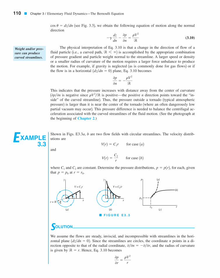
Shown in Figs. E3.3a, b are two flow fields with circular streamlines. The velocity distrib-utions are
and
where and are constant. Determine the pressure distributions, for each, giventhat at r � r0.p � p0
p � p1r2,C2C1
V1r2 �C2
r for case 1b2
V1r2 � C1r for case 1a2
SOLUTION
We assume the flows are steady, inviscid, and incompressible with streamlines in the hori-zontal plane Since the streamlines are circles, the coordinate n points in a di-rection opposite to that of the radial coordinate, and the radius of curvatureis given by Hence, Eq. 3.10 becomes
0p
0r�rV 2
r
r � r.0�0n � �0�0r,
1dz�dn � 02.
y
r = � n
(a)
V = C1r V = C2/r
y
(b)
xx
p
p0
r0
(a)
(b)
(c)r
� F I G U R E E 3 . 3
Weight and/or pres-sure can producecurved streamlines.
7708d_c03_110 8/10/01 3:13 PM Page 110 mac120 mac120:1st shift:
If we multiply Eq. 3.10 by dn, use the fact that if s is constant, and integrateacross the streamline 1in the n direction2 we obtain
(3.11)
To complete the indicated integrations, we must know how the density varies with pres-sure and how the fluid speed and radius of curvature vary with n. For incompressible flowthe density is constant and the integration involving the pressure term gives simply Weare still left, however, with the integration of the second term in Eq. 3.11. Without knowingthe n dependence in and this integration cannot be completed.
Thus, the final form of Newton’s second law applied across the streamlines for steady,inviscid, incompressible flow is
(3.12)
As with the Bernoulli equation, we must be careful that the assumptions involved in the de-rivation of this equation are not violated when it is used.
p � r � V 2
r dn � yz � constant across the streamline
r � r1s, n2V � V1s, n2p�r.
� dpr
� � V 2
r dn � gz � constant across the streamline
0p�0n � dp�dn
3.4 Physical Interpretation � 111
For case 1a2 this gives
while for case 1b2 it gives
For either case the pressure increases as r increases since Integration of theseequations with respect to r, starting with a known pressure at gives
(Ans)
for case 1a2 and
(Ans)
for case 1b2. These pressure distributions are sketched in Fig. E3.3c. The pressure distribu-tions needed to balance the centrifugal accelerations in cases 1a2 and 1b2 are not the same be-cause the velocity distributions are different. In fact for case 1a2 the pressure increases with-out bound as while for case 1b2 the pressure approaches a finite value as Thestreamline patterns are the same for each case, however.
Physically, case 1a2 represents rigid body rotation 1as obtained in a can of water on aturntable after it has been “spun up”2 and case 1b2 represents a free vortex 1an approximationof a tornado or the swirl of water in a drain, the “bathtub vortex”2. (See the photograph atthe beginning of Chapter 4 for an approximation of this type of flow.)
r S �.r S �,
p �1
2 rC 2
2 a 1
r 02 �
1
r 2b � p0
p �1
2 rC 1
2 1r 2 � r 022 � p0
r � r0,p � p0
0p�0r 7 0.
0p
0r�rC 2
2
r 3
0p
0r� rC 1
2r
The sum of pres-sure, elevation, andvelocity effects isconstant acrossstreamlines.
V3.2 Free vortex
3.4 Physical Interpretation
In the previous two sections, we developed the basic equations governing fluid motion un-der a fairly stringent set of restrictions. In spite of the numerous assumptions imposed onthese flows, a variety of flows can be readily analyzed with them. A physical interpretation
7708d_c03_111 8/10/01 3:13 PM Page 111 mac120 mac120:1st shift:
of the equations will be of help in understanding the processes involved. To this end, werewrite Eqs. 3.7 and 3.12 here and interpret them physically. Application of alongand normal to the streamline results in
(3.13)
and
(3.14)
The following basic assumptions were made to obtain these equations: The flow is steadyand the fluid is inviscid and incompressible. In practice none of these assumptions is exactlytrue.
A violation of one or more of the above assumptions is a common cause for obtainingan incorrect match between the “real world” and solutions obtained by use of the Bernoulliequation. Fortunately, many “real-world” situations are adequately modeled by the use ofEqs. 3.13 and 3.14 because the flow is nearly steady and incompressible and the fluid be-haves as if it were nearly inviscid.
The Bernoulli equation was obtained by integration of the equation of motion alongthe “natural” coordinate direction of the streamline. To produce an acceleration, there mustbe an unbalance of the resultant forces, of which only pressure and gravity were consideredto be important. Thus, there are three processes involved in the flow—mass times accelera-tion 1the term2, pressure 1the p term2, and weight 1the term2.
Integration of the equation of motion to give Eq. 3.13 actually corresponds to the work-energy principle often used in the study of dynamics [see any standard dynamics text 1Ref. 12].This principle results from a general integration of the equations of motion for an object ina way very similar to that done for the fluid particle in Section 3.2. With certain assump-tions, a statement of the work-energy principle may be written as follows:
The work done on a particle by all forces acting on the particle is equal to the changeof the kinetic energy of the particle.
The Bernoulli equation is a mathematical statement of this principle.As the fluid particle moves, both gravity and pressure forces do work on the particle.
Recall that the work done by a force is equal to the product of the distance the particle trav-els times the component of force in the direction of travel 1i.e., 2. The terms and p in Eq. 3.13 are related to the work done by the weight and pressure forces, respec-tively. The remaining term, is obviously related to the kinetic energy of the particle.In fact, an alternate method of deriving the Bernoulli equation is to use the first and secondlaws of thermodynamics 1the energy and entropy equations2, rather than Newton’s secondlaw. With the appropriate restrictions, the general energy equation reduces to the Bernoulliequation. This approach is discussed in Section 5.4.
An alternate but equivalent form of the Bernoulli equation is obtained by dividing eachterm of Eq. 3.7 by the specific weight, to obtain
Each of the terms in this equation has the units of energy per weight or length1feet, meters2 and represents a certain type of head.
The elevation term, z, is related to the potential energy of the particle and is called theelevation head. The pressure term, is called the pressure head and represents the heightof a column of the fluid that is needed to produce the pressure p. The velocity term, V
2�2g,p�g,
1LF�F � L2
p
g�
V 2
2g� z � constant on a streamline
g,
rV
2�2,
gzwork � F � d
gzrV
2�2
p � r � V 2
r dn � gz � constant across the streamline
p � 12rV
2 � gz � constant along the streamline
F � ma
112 � Chapter 3 / Elementary Fluid Dynamics—The Bernoulli Equation
The Bernoulliequation can bewritten in terms ofheights calledheads.
7708d_c03_112 8/10/01 3:14 PM Page 112 mac120 mac120:1st shift:
is the velocity head and represents the vertical distance needed for the fluid to fall freely1neglecting friction2 if it is to reach velocity V from rest. The Bernoulli equation states thatthe sum of the pressure head, the velocity head, and the elevation head is constant along astreamline.
3.4 Physical Interpretation � 113
EXAMPLE3.4
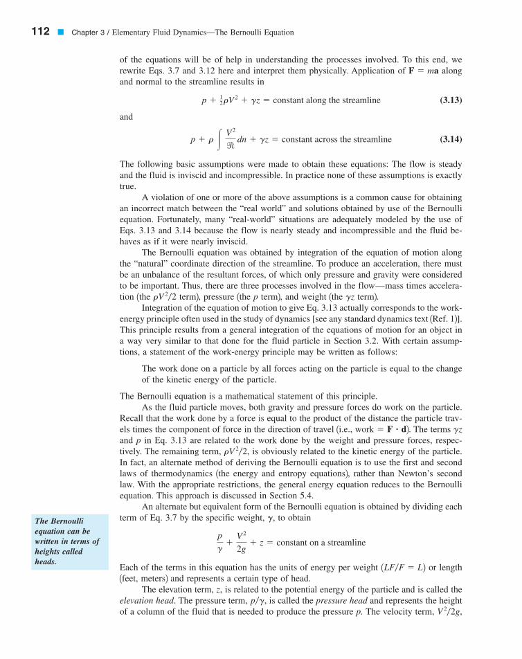
Consider the flow of water from the syringe shown in Fig. E3.4. A force applied to the plungerwill produce a pressure greater than atmospheric at point 112 within the syringe. The waterflows from the needle, point 122, with relatively high velocity and coasts up to point 132 at thetop of its trajectory. Discuss the energy of the fluid at points 112, 122, and 132 by using theBernoulli equation.
Energy Type
Kinetic Potential PressurePoint p
1 Small Zero Large2 Large Small Zero3 Zero Large Zero
GzRV 2�2
A net force is required to accelerate any mass. For steady flow the acceleration can beinterpreted as arising from two distinct occurrences—a change in speed along the stream-line and a change in direction if the streamline is not straight. Integration of the equation ofmotion along the streamline accounts for the change in speed 1kinetic energy change2 and re-sults in the Bernoulli equation. Integration of the equation of motion normal to the stream-line accounts for the centrifugal acceleration and results in Eq. 3.14.1V 2�r2
g
F
(1)
(2)
(3)
SOLUTION
If the assumptions 1steady, inviscid, incompressible flow2 of the Bernoulli equation are ap-proximately valid, it then follows that the flow can be explained in terms of the partition ofthe total energy of the water. According to Eq. 3.13 the sum of the three types of energy 1ki-netic, potential, and pressure2 or heads 1velocity, elevation, and pressure2 must remain con-stant. The following table indicates the relative magnitude of each of these energies at thethree points shown in the figure.
The motion results in 1or is due to2 a change in the magnitude of each type of energyas the fluid flows from one location to another. An alternate way to consider this flow is asfollows. The pressure gradient between 112 and 122 produces an acceleration to eject the wa-ter from the needle. Gravity acting on the particle between 122 and 132 produces a decelera-tion to cause the water to come to a momentary stop at the top of its flight.
If friction 1viscous2 effects were important, there would be an energy loss between112 and 132 and for the given the water would not be able to reach the height indicated inthe figure. Such friction may arise in the needle 1see Chapter 8 on pipe flow2 or betweenthe water stream and the surrounding air 1see Chapter 9 on external flow2.
p1
� F I G U R E E 3 . 4
7708d_c03_113 8/10/01 3:14 PM Page 113 mac120 mac120:1st shift:
When a fluid particle travels along a curved path, a net force directed toward the cen-ter of curvature is required. Under the assumptions valid for Eq. 3.14, this force may be eithergravity or pressure, or a combination of both. In many instances the streamlines are nearlystraight so that centrifugal effects are negligible and the pressure variation acrossthe streamlines is merely hydrostatic 1because of gravity alone2, even though the fluid is inmotion.
1r � � 2
114 � Chapter 3 / Elementary Fluid Dynamics—The Bernoulli Equation
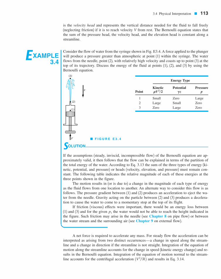
EXAMPLE3.5
Consider the inviscid, incompressible, steady flow shown in Fig. E3.5. From section A to Bthe streamlines are straight, while from C to D they follow circular paths. Describe the pres-sure variation between points 112 and 122 and points 132 and 142.
SOLUTION
With the above assumptions and the fact that for the portion from A to B, Eq. 3.14becomes
The constant can be determined by evaluating the known variables at the two locations us-ing and to give
(Ans)
Note that since the radius of curvature of the streamline is infinite, the pressure variation inthe vertical direction is the same as if the fluid were stationary.
However, if we apply Eq. 3.14 between points 132 and 142 we obtain 1using 2
With and this becomes
(Ans)
To evaluate the integral, we must know the variation of V and with z. Even without thisdetailed information we note that the integral has a positive value. Thus, the pressure at 132 isless than the hydrostatic value, by an amount equal to This lowerpressure, caused by the curved streamline, is necessary to accelerate the fluid around thecurved path.
Note that we did not apply the Bernoulli equation 1Eq. 3.132 across the streamlinesfrom 112 to 122 or 132 to 142. Rather we used Eq. 3.14. As is discussed in Section 3.8, applica-tion of the Bernoulli equation across streamlines 1rather than along them2 may lead to seri-ous errors.
r � z4
z3 1V 2�r2 dz.gh4–3,
r
p3 � gh4–3 � r �z4
z3
V 2
r dz
z4 � z3 � h4–3p4 � 0
p4 � r �z4
z3
V 2
r 1�dz2 � gz4 � p3 � gz3
dn � �dz
p1 � p2 � g1z2 � z12 � p2 � gh2–1
z2 � h2–1p2 � 0 1gage2, z1 � 0,
p � gz � constant
r � �
zg
(2)
(1)
h2-1
A B
C D�
Free surface(p = 0)
n
h4-3
(4)
(3)
^
� F I G U R E E 3 . 5
The pressure varia-tion across straightstreamlines is hy-drostatic.
7708d_c03_114 8/10/01 3:14 PM Page 114 mac120 mac120:1st shift:
The third term in Eq. 3.13, is termed the hydrostatic pressure, in obvious regard tothe hydrostatic pressure variation discussed in Chapter 2. It is not actually a pressure butdoes represent the change in pressure possible due to potential energy variations of the fluidas a result of elevation changes.
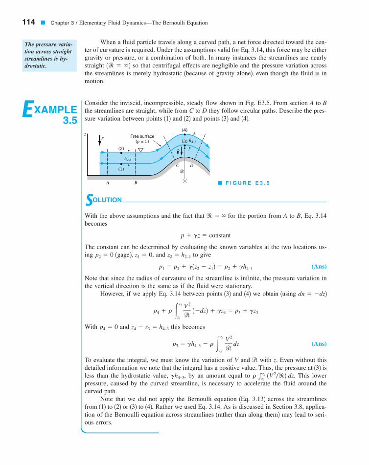
The second term in the Bernoulli equation, is termed the dynamic pressure. Itsinterpretation can be seen in Fig. 3.4 by considering the pressure at the end of a small tubeinserted into the flow and pointing upstream. After the initial transient motion has died out,the liquid will fill the tube to a height of H as shown. The fluid in the tube, including thatat its tip, 122, will be stationary. That is, or point 122 is a stagnation point.
If we apply the Bernoulli equation between points 112 and 122, using and as-suming that we find that
Hence, the pressure at the stagnation point is greater than the static pressure, by an amountthe dynamic pressure.
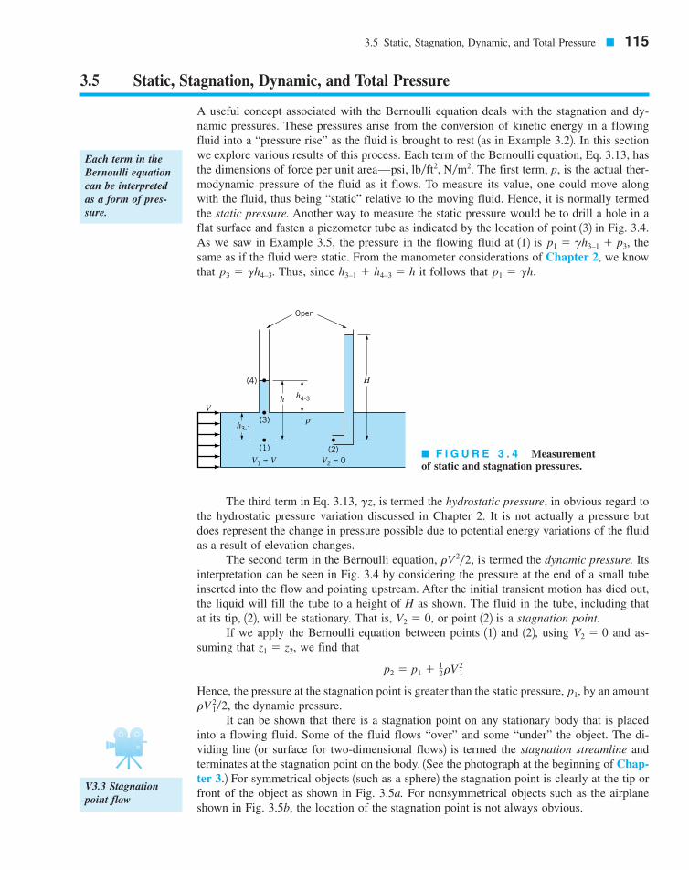
It can be shown that there is a stagnation point on any stationary body that is placedinto a flowing fluid. Some of the fluid flows “over” and some “under” the object. The di-viding line 1or surface for two-dimensional flows2 is termed the stagnation streamline andterminates at the stagnation point on the body. 1See the photograph at the beginning of Chap-ter 3.2 For symmetrical objects 1such as a sphere2 the stagnation point is clearly at the tip orfront of the object as shown in Fig. 3.5a. For nonsymmetrical objects such as the airplaneshown in Fig. 3.5b, the location of the stagnation point is not always obvious.
rV
21�2,
p1,
p2 � p1 � 12rV
21
z1 � z2,V2 � 0
V2 � 0,
rV 2�2,
gz,
3.5 Static, Stagnation, Dynamic, and Total Pressure � 115
3.5 Static, Stagnation, Dynamic, and Total Pressure
A useful concept associated with the Bernoulli equation deals with the stagnation and dy-namic pressures. These pressures arise from the conversion of kinetic energy in a flowingfluid into a “pressure rise” as the fluid is brought to rest 1as in Example 3.22. In this sectionwe explore various results of this process. Each term of the Bernoulli equation, Eq. 3.13, hasthe dimensions of force per unit area—psi, The first term, p, is the actual ther-modynamic pressure of the fluid as it flows. To measure its value, one could move alongwith the fluid, thus being “static” relative to the moving fluid. Hence, it is normally termedthe static pressure. Another way to measure the static pressure would be to drill a hole in aflat surface and fasten a piezometer tube as indicated by the location of point 132 in Fig. 3.4.As we saw in Example 3.5, the pressure in the flowing fluid at 112 is thesame as if the fluid were static. From the manometer considerations of Chapter 2, we knowthat Thus, since it follows that p1 � gh.h3–1 � h4–3 � hp3 � gh4–3.
p1 � gh3–1 � p3,
lb�ft2, N�m2.
V3.3 Stagnationpoint flow
Each term in theBernoulli equationcan be interpretedas a form of pres-sure.
� F I G U R E 3 . 4 Measurementof static and stagnation pressures.
(1) (2)
(3)
(4)
h3-1
h h4-3
ρ
Open
H
V
V1 = V V2 = 0
7708d_c03_115 8/10/01 3:15 PM Page 115 mac120 mac120:1st shift:
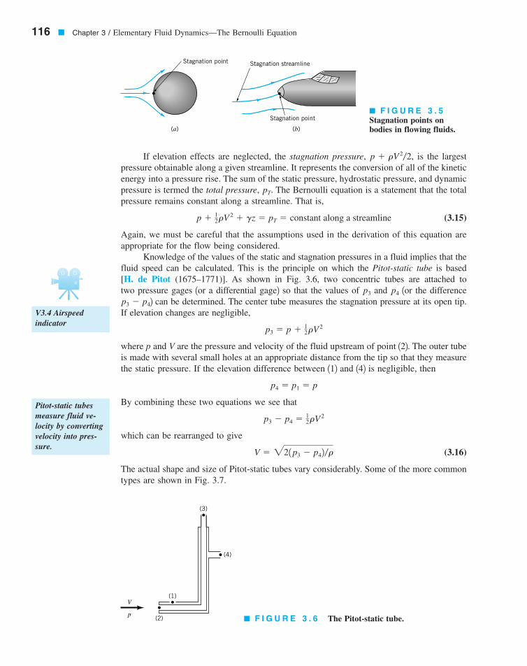
If elevation effects are neglected, the stagnation pressure, is the largestpressure obtainable along a given streamline. It represents the conversion of all of the kineticenergy into a pressure rise. The sum of the static pressure, hydrostatic pressure, and dynamicpressure is termed the total pressure, The Bernoulli equation is a statement that the totalpressure remains constant along a streamline. That is,
(3.15)
Again, we must be careful that the assumptions used in the derivation of this equation areappropriate for the flow being considered.
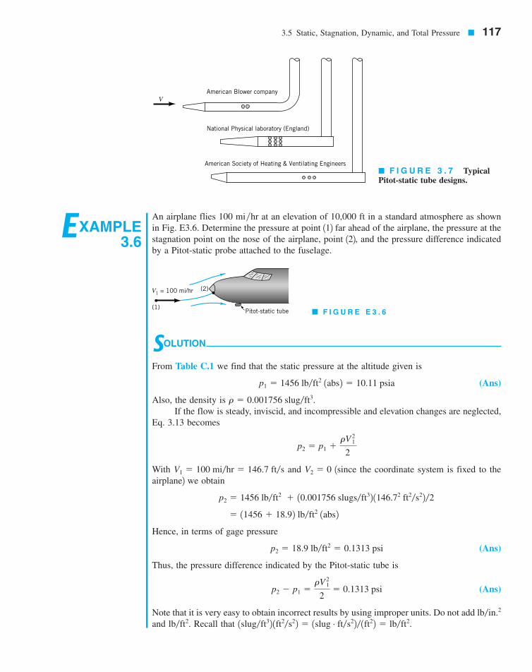
Knowledge of the values of the static and stagnation pressures in a fluid implies that thefluid speed can be calculated. This is the principle on which the Pitot-static tube is based [H. de Pitot (1675–1771)]. As shown in Fig. 3.6, two concentric tubes are attached to two pressure gages 1or a differential gage2 so that the values of and 1or the difference
2 can be determined. The center tube measures the stagnation pressure at its open tip.If elevation changes are negligible,
where p and V are the pressure and velocity of the fluid upstream of point 122. The outer tubeis made with several small holes at an appropriate distance from the tip so that they measurethe static pressure. If the elevation difference between 112 and 142 is negligible, then
By combining these two equations we see that
which can be rearranged to give
(3.16)
The actual shape and size of Pitot-static tubes vary considerably. Some of the more commontypes are shown in Fig. 3.7.
V � 221p3 � p42�r
p3 � p4 � 12rV
2
p4 � p1 � p
p3 � p � 12rV
2
p3 � p4
p4p3
p � 12rV
2 � gz � pT � constant along a streamline
pT.
p � rV 2�2,
116 � Chapter 3 / Elementary Fluid Dynamics—The Bernoulli Equation
Stagnation point
(a)
Stagnation streamline
Stagnation point
(b)
� F I G U R E 3 . 5Stagnation points on bodies in flowing fluids.
Pitot-static tubesmeasure fluid ve-locity by convertingvelocity into pres-sure.
� F I G U R E 3 . 6 The Pitot-static tube.
V
p
(1)
(2)
(4)
(3)
V3.4 Airspeed indicator
7708d_c03_116 8/13/01 6:40 PM Page 116
3.5 Static, Stagnation, Dynamic, and Total Pressure � 117
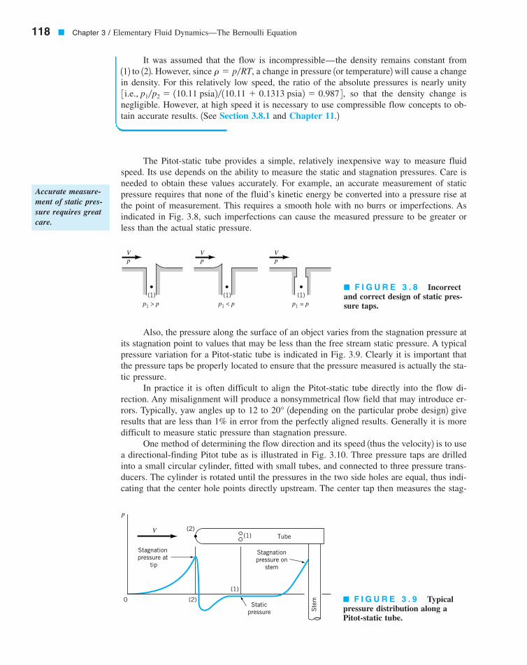
EXAMPLE3.6
An airplane flies 100 mi�hr at an elevation of 10,000 ft in a standard atmosphere as shownin Fig. E3.6. Determine the pressure at point 112 far ahead of the airplane, the pressure at thestagnation point on the nose of the airplane, point 122, and the pressure difference indicatedby a Pitot-static probe attached to the fuselage.
VAmerican Blower company
National Physical laboratory (England)
American Society of Heating & Ventilating Engineers� F I G U R E 3 . 7 TypicalPitot-static tube designs.
SOLUTION
From Table C.1 we find that the static pressure at the altitude given is
(Ans)
Also, the density is If the flow is steady, inviscid, and incompressible and elevation changes are neglected,
Eq. 3.13 becomes
With and 1since the coordinate system is fixed to theairplane2 we obtain
Hence, in terms of gage pressure
(Ans)
Thus, the pressure difference indicated by the Pitot-static tube is
(Ans)
Note that it is very easy to obtain incorrect results by using improper units. Do not add and Recall that 1slug�ft32 1ft2�s22 � 1slug # ft�s22� 1ft22 � lb�ft2.lb�ft2.
lb�in.2
p2 � p1 �rV 2
1
2� 0.1313 psi
p2 � 18.9 lb�ft2 � 0.1313 psi
� 11456 � 18.92 lb�ft2 1abs2
p2 � 1456 lb�ft2 � 10.001756 slugs�ft32 1146.72 ft2�s22�2
V2 � 0V1 � 100 mi�hr � 146.7 ft�s
p2 � p1 �rV 2
1
2
r � 0.001756 slug�ft3.
p1 � 1456 lb�ft2 1abs2 � 10.11 psia
V1 = 100 mi/hr (2)
(1)Pitot-static tube � F I G U R E E 3 . 6
7708d_c03_117 8/10/01 3:25 PM Page 117 mac120 mac120:1st shift:
The Pitot-static tube provides a simple, relatively inexpensive way to measure fluidspeed. Its use depends on the ability to measure the static and stagnation pressures. Care isneeded to obtain these values accurately. For example, an accurate measurement of staticpressure requires that none of the fluid’s kinetic energy be converted into a pressure rise atthe point of measurement. This requires a smooth hole with no burrs or imperfections. Asindicated in Fig. 3.8, such imperfections can cause the measured pressure to be greater orless than the actual static pressure.
118 � Chapter 3 / Elementary Fluid Dynamics—The Bernoulli Equation
It was assumed that the flow is incompressible—the density remains constant from112 to 122. However, since a change in pressure 1or temperature2 will cause a changein density. For this relatively low speed, the ratio of the absolute pressures is nearly unity
so that the density change isnegligible. However, at high speed it is necessary to use compressible flow concepts to ob-tain accurate results. 1See Section 3.8.1 and Chapter 11.2
3 i.e., p1�p2 � 110.11 psia2� 110.11 � 0.1313 psia2 � 0.987 4 ,
r � p�RT,
Accurate measure-ment of static pres-sure requires greatcare.
Also, the pressure along the surface of an object varies from the stagnation pressure atits stagnation point to values that may be less than the free stream static pressure. A typicalpressure variation for a Pitot-static tube is indicated in Fig. 3.9. Clearly it is important thatthe pressure taps be properly located to ensure that the pressure measured is actually the sta-tic pressure.
In practice it is often difficult to align the Pitot-static tube directly into the flow di-rection. Any misalignment will produce a nonsymmetrical flow field that may introduce er-rors. Typically, yaw angles up to 12 to 1depending on the particular probe design2 giveresults that are less than 1% in error from the perfectly aligned results. Generally it is moredifficult to measure static pressure than stagnation pressure.
One method of determining the flow direction and its speed 1thus the velocity2 is to usea directional-finding Pitot tube as is illustrated in Fig. 3.10. Three pressure taps are drilledinto a small circular cylinder, fitted with small tubes, and connected to three pressure trans-ducers. The cylinder is rotated until the pressures in the two side holes are equal, thus indi-cating that the center hole points directly upstream. The center tap then measures the stag-
20°
� F I G U R E 3 . 8 Incorrectand correct design of static pres-sure taps.
� F I G U R E 3 . 9 Typicalpressure distribution along aPitot-static tube.
Vp
Vp
Vp
(1)p1 = p
(1)p1 < p
(1)p1 > p
V
Stagnationpressure on
stem
Staticpressure S
tem
Tube(1)
(1)
(2)
(2)
Stagnationpressure at
tip
0
p
7708d_c03_118 8/10/01 3:26 PM Page 118 mac120 mac120:1st shift:
nation pressure. The two side holes are located at a specific angle so that theymeasure the static pressure. The speed is then obtained from
The above discussion is valid for incompressible flows. At high speeds, compressibil-ity becomes important 1the density is not constant2 and other phenomena occur. Some of theseideas are discussed in Section 3.8, while others 1such as shockwaves for supersonic Pitot-tube applications2 are discussed in Chapter 11.
The concepts of static, dynamic, stagnation, and total pressure are useful in a varietyof flow problems. These ideas are used more fully in the remainder of the book.
V � 321p2 � p12�r 4 1�2.1b � 29.5°2
3.6 Examples of Use of the Bernoulli Equation � 119
Many velocity mea-suring devices usePitot-static tubeprinciples.
β
βθ
V
p(1)
(2)
(3) If = 0θ
ρ
p1 = p3 = p
p2 = p + V21_2
(2) (4)
(1)
(3)
V
d
(5)
H
�
h z
(2)
� F I G U R E 3 . 1 0 Cross sec-tion of a directional-finding Pitot-static tube.
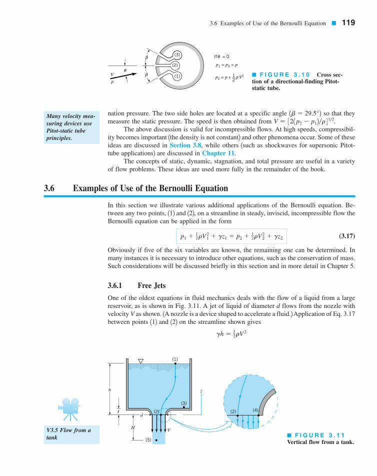
� F I G U R E 3 . 1 1Vertical flow from a tank.
3.6 Examples of Use of the Bernoulli Equation
In this section we illustrate various additional applications of the Bernoulli equation. Be-tween any two points, 112 and 122, on a streamline in steady, inviscid, incompressible flow theBernoulli equation can be applied in the form
(3.17)
Obviously if five of the six variables are known, the remaining one can be determined. Inmany instances it is necessary to introduce other equations, such as the conservation of mass.Such considerations will be discussed briefly in this section and in more detail in Chapter 5.
3.6.1 Free Jets
One of the oldest equations in fluid mechanics deals with the flow of a liquid from a largereservoir, as is shown in Fig. 3.11. A jet of liquid of diameter d flows from the nozzle withvelocity V as shown. 1A nozzle is a device shaped to accelerate a fluid.2Application of Eq. 3.17between points 112 and 122 on the streamline shown gives
gh � 12rV
2
p1 � 12rV
21 � gz1 � p2 � 1
2rV22 � gz2
V3.5 Flow from atank
7708d_c03_119 8/10/01 3:26 PM Page 119 mac120 mac120:1st shift:
We have used the facts that the reservoir is large open to the at-mosphere and the fluid leaves as a “free jet” Thus, we obtain
(3.18)
which is the modern version of a result obtained in 1643 by Torricelli 11608–16472, an Ital-ian physicist.
The fact that the exit pressure equals the surrounding pressure can be seenby applying as given by Eq. 3.14, across the streamlines between 122 and 142. If thestreamlines at the tip of the nozzle are straight it follows that Since 142 ison the surface of the jet, in contact with the atmosphere, we have Thus, also.Since 122 is an arbitrary point in the exit plane of the nozzle, it follows that the pressure isatmospheric across this plane. Physically, since there is no component of the weight force oracceleration in the normal 1horizontal2 direction, the pressure is constant in that direction.
Once outside the nozzle, the stream continues to fall as a free jet with zero pressurethroughout and as seen by applying Eq. 3.17 between points 112 and 152, the speedincreases according to
where H is the distance the fluid has fallen outside the nozzle.Equation 3.18 could also be obtained by writing the Bernoulli equation between points
132 and 142 using the fact that Also, since it is far from the nozzle, andfrom hydrostatics,
Recall from physics or dynamics that any object dropped from rest through a distanceh in a vacuum will obtain the speed the same as the liquid leaving the nozzle.This is consistent with the fact that all of the particle’s potential energy is converted to ki-netic energy, provided viscous 1friction2 effects are negligible. In terms of heads, the eleva-tion head at point 112 is converted into the velocity head at point 122. Recall that for the caseshown in Fig. 3.11 the pressure is the same 1atmospheric2 at points 112 and 122.
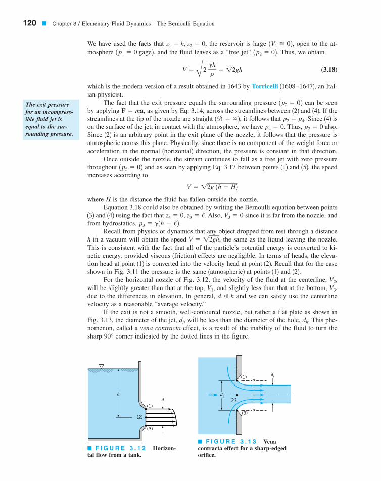
For the horizontal nozzle of Fig. 3.12, the velocity of the fluid at the centerline,will be slightly greater than that at the top, and slightly less than that at the bottom,due to the differences in elevation. In general, and we can safely use the centerlinevelocity as a reasonable “average velocity.”
If the exit is not a smooth, well-contoured nozzle, but rather a flat plate as shown inFig. 3.13, the diameter of the jet, will be less than the diameter of the hole, This phe-nomenon, called a vena contracta effect, is a result of the inability of the fluid to turn thesharp corner indicated by the dotted lines in the figure.90°
dh.dj,
d � hV3,V1,V2,
V � 12gh,
p3 � g1h � /2.V3 � 0z4 � 0, z3 � /.
V � 12g 1h � H2
1p5 � 02
p2 � 0p4 � 0.p2 � p4.1r � � 2,
F � ma,1p2 � 02
V � B2 gh
r� 12gh
1p2 � 02.1p1 � 0 gage2,1V1 � 02,z1 � h, z2 � 0,
120 � Chapter 3 / Elementary Fluid Dynamics—The Bernoulli Equation
hd
(1)
(2)
(3)
dj
dh(2)
(1)
(3)a
a
The exit pressurefor an incompress-ible fluid jet isequal to the sur-rounding pressure.
� F I G U R E 3 . 1 2 Horizon-tal flow from a tank.
� F I G U R E 3 . 1 3 Vena contracta effect for a sharp-edgedorifice.
7708d_c03_120 8/13/01 1:35 AM Page 120
Since the streamlines in the exit plane are curved the pressure across themis not constant. It would take an infinite pressure gradient across the streamlines to cause thefluid to turn a “sharp” corner The highest pressure occurs along the centerline at122 and the lowest pressure, is at the edge of the jet. Thus, the assumption ofuniform velocity with straight streamlines and constant pressure is not valid at the exit plane.It is valid, however, in the plane of the vena contracta, section a–a. The uniform velocity as-sumption is valid at this section provided as is discussed for the flow from the nozzleshown in Fig. 3.12.
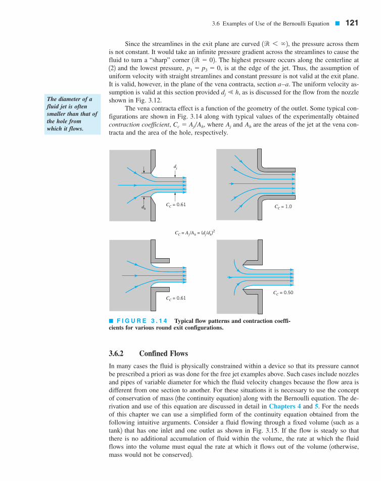
The vena contracta effect is a function of the geometry of the outlet. Some typical con-figurations are shown in Fig. 3.14 along with typical values of the experimentally obtainedcontraction coefficient, where and are the areas of the jet at the vena con-tracta and the area of the hole, respectively.
AhAjCc � Aj�Ah,
dj � h,
p1 � p3 � 0,1r � 02.
1r 6 � 2,
3.6 Examples of Use of the Bernoulli Equation � 121
3.6.2 Confined Flows
In many cases the fluid is physically constrained within a device so that its pressure cannotbe prescribed a priori as was done for the free jet examples above. Such cases include nozzlesand pipes of variable diameter for which the fluid velocity changes because the flow area isdifferent from one section to another. For these situations it is necessary to use the conceptof conservation of mass 1the continuity equation2 along with the Bernoulli equation. The de-rivation and use of this equation are discussed in detail in Chapters 4 and 5. For the needsof this chapter we can use a simplified form of the continuity equation obtained from thefollowing intuitive arguments. Consider a fluid flowing through a fixed volume 1such as atank2 that has one inlet and one outlet as shown in Fig. 3.15. If the flow is steady so thatthere is no additional accumulation of fluid within the volume, the rate at which the fluidflows into the volume must equal the rate at which it flows out of the volume 1otherwise,mass would not be conserved2.
� F I G U R E 3 . 1 4 Typical flow patterns and contraction coeffi-cients for various round exit configurations.
The diameter of afluid jet is oftensmaller than that ofthe hole fromwhich it flows.
dh
dj
CC = 0.61
CC = 0.61CC = 0.50
CC = 1.0
CC = Aj /Ah = (dj /dh)2
7708d_c03_121 8/10/01 3:26 PM Page 121 mac120 mac120:1st shift:
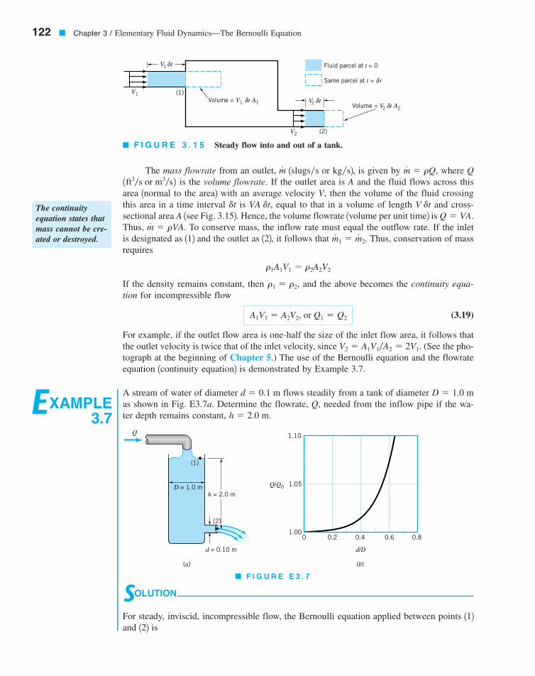
The mass flowrate from an outlet, 1slugs�s or kg�s2, is given by where Qis the volume flowrate. If the outlet area is A and the fluid flows across this
area 1normal to the area2 with an average velocity V, then the volume of the fluid crossingthis area in a time interval is equal to that in a volume of length and cross-sectional area A 1see Fig. 3.152. Hence, the volume flowrate 1volume per unit time2 is Thus, To conserve mass, the inflow rate must equal the outflow rate. If the inletis designated as 112 and the outlet as 122, it follows that Thus, conservation of massrequires
If the density remains constant, then and the above becomes the continuity equa-tion for incompressible flow
(3.19)
For example, if the outlet flow area is one-half the size of the inlet flow area, it follows thatthe outlet velocity is twice that of the inlet velocity, since (See the pho-tograph at the beginning of Chapter 5.) The use of the Bernoulli equation and the flowrateequation 1continuity equation2 is demonstrated by Example 3.7.
V2 � A1V1�A2 � 2V1.
A1V1 � A2V2, or Q1 � Q2
r1 � r2,
r1A1V1 � r2A2V2
m#
1 � m#
2.m#
� rVA.Q � VA.
V dtVA dt,dt
1ft3�s or m3�s2m#
� rQ,m#
122 � Chapter 3 / Elementary Fluid Dynamics—The Bernoulli Equation
V1
V1 t
(1)Volume = V1 t A1
V2 (2)
Volume = V2 t A2
Same parcel at t = t
Fluid parcel at t = 0δ
δ δV2 t
δ
δ
� F I G U R E 3 . 1 5 Steady flow into and out of a tank.
EXAMPLE3.7
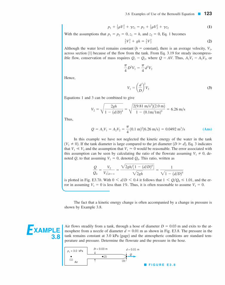
A stream of water of diameter flows steadily from a tank of diameter as shown in Fig. E3.7a. Determine the flowrate, Q, needed from the inflow pipe if the wa-ter depth remains constant, .h � 2.0 m
D � 1.0 md � 0.1 m
SOLUTION
For steady, inviscid, incompressible flow, the Bernoulli equation applied between points 112and 122 is
Q 1.10
1.05
1.000 0.2 0.4 0.6 0.8
d/D
Q/Q0
(a) (b)
d = 0.10 m
h = 2.0 mD = 1.0 m
(1)
(2)
� F I G U R E E 3 . 7
The continuityequation states thatmass cannot be cre-ated or destroyed.
7708d_c03_122 8/10/01 3:27 PM Page 122 mac120 mac120:1st shift:
EXAMPLE3.8
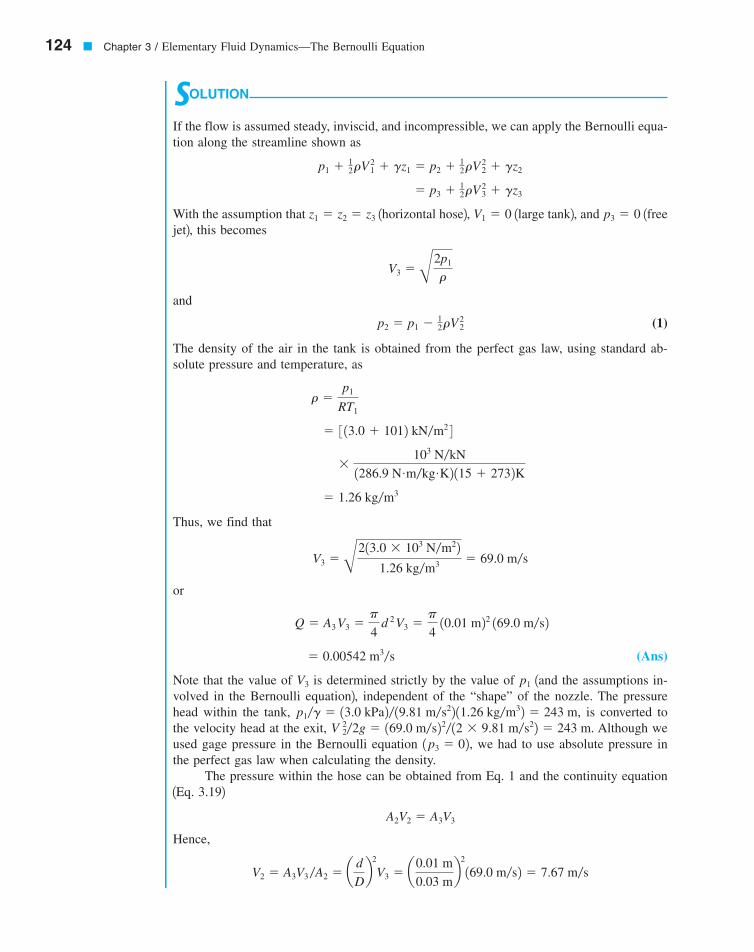
Air flows steadily from a tank, through a hose of diameter and exits to the at-mosphere from a nozzle of diameter as shown in Fig. E3.8. The pressure in thetank remains constant at 3.0 kPa 1gage2 and the atmospheric conditions are standard tem-perature and pressure. Determine the flowrate and the pressure in the hose.
d � 0.01 mD � 0.03 m
3.6 Examples of Use of the Bernoulli Equation � 123
The fact that a kinetic energy change is often accompanied by a change in pressure isshown by Example 3.8.
(1)
With the assumptions that and Eq. 1 becomes
(2)
Although the water level remains constant 1 constant2, there is an average velocity,across section 112 because of the flow from the tank. From Eq. 3.19 for steady incompress-ible flow, conservation of mass requires where Thus, or
Hence,
(3)
Equations 1 and 3 can be combined to give
Thus,
(Ans)
In this example we have not neglected the kinetic energy of the water in the tankIf the tank diameter is large compared to the jet diameter Eq. 3 indicates
that and the assumption that would be reasonable. The error associated withthis assumption can be seen by calculating the ratio of the flowrate assuming de-noted Q, to that assuming denoted This ratio, written as
is plotted in Fig. E3.7b. With it follows that and the er-ror in assuming is less than 1%. Thus, it is often reasonable to assume V1 � 0.V1 � 0
1 6 Q�Q0 � 1.01,0 6 d�D 6 0.4
Q
Q0�
V2
V2 0 D��
�22gh� 31 � 1d�D24 422gh
�121 � 1d�D24
Q0.V1 � 0,V1 � 0,
V1 � 0V1 � V2
1D d2,1V1 � 02.
Q � A1V1 � A2V2 �p
4 10.1 m2216.26 m�s2 � 0.0492 m3�s
V2 � B 2gh
1 � 1d�D24 � B219.81 m�s22 12.0 m21 � 10.1m�1m24 � 6.26 m�s
V1 � a d
Db2
V2
p
4 D2V1 �
p
4 d2V2
A1V1 � A2V2,Q � AV.Q1 � Q2,
V1,h �
12V 2
1 gh � 12V 2
2
z2 � 0,p1 � p2 � 0, z1 � h,
p1 12rV
21 gz1 � p2 1
2rV22 gz2
p1 = 3.0 kPa
(1)Air
D = 0.03 m
(2)
(3)
d = 0.01 m
Q
� F I G U R E E 3 . 8
7708d_c03_123 8/10/01 3:27 PM Page 123 mac120 mac120:1st shift:
124 � Chapter 3 / Elementary Fluid Dynamics—The Bernoulli Equation
SOLUTION
If the flow is assumed steady, inviscid, and incompressible, we can apply the Bernoulli equa-tion along the streamline shown as
With the assumption that 1horizontal hose2, 1large tank2, and 1freejet2, this becomes
and
(1)
The density of the air in the tank is obtained from the perfect gas law, using standard ab-solute pressure and temperature, as
Thus, we find that
or
(Ans)
Note that the value of is determined strictly by the value of 1and the assumptions in-volved in the Bernoulli equation2, independent of the “shape” of the nozzle. The pressurehead within the tank, is converted tothe velocity head at the exit, Although weused gage pressure in the Bernoulli equation we had to use absolute pressure inthe perfect gas law when calculating the density.
The pressure within the hose can be obtained from Eq. 1 and the continuity equation1Eq. 3.192
Hence,
V2 � A3V3 �A2 � a d
Db2
V3 � a0.01 m
0.03 mb2169.0 m�s2 � 7.67 m�s
A2V2 � A3V3
1p3 � 02,V 22�2g � 169.0 m�s22� 12 � 9.81 m�s22 � 243 m.p1�g � 13.0 kPa2� 19.81 m�s22 11.26 kg�m32 � 243 m,
p1V3
� 0.00542 m3�s
Q � A3 V3 �p
4 d 2V3 �
p
4 10.01 m22 169.0 m�s2
V3 � B213.0 � 103 N�m221.26 kg�m3 � 69.0 m�s
� 1.26 kg�m3
�103 N�kN
1286.9 N�m�kg�K2 115 � 2732K
� 3 13.0 � 1012 kN�m2 4 r �
p1
RT1
p2 � p1 � 12rV
22
V3 � B2p1
r
p3 � 0V1 � 0z1 � z2 � z3
� p3 � 12rV
23 � gz3
p1 � 12rV
21 � gz1 � p2 � 1
2rV22 � gz2
7708d_c03_124 8/10/01 3:27 PM Page 124 mac120 mac120:1st shift:
In many situations the combined effects of kinetic energy, pressure, and gravity areimportant. Example 3.9 illustrates this.
3.6 Examples of Use of the Bernoulli Equation � 125
and from Eq. 1
(Ans)
In the absence of viscous effects the pressure throughout the hose is constant and equalto Physically, the decreases in pressure from to to accelerate the air and increaseits kinetic energy from zero in the tank to an intermediate value in the hose and finally to itsmaximum value at the nozzle exit. Since the air velocity in the nozzle exit is nine times thatin the hose, most of the pressure drop occurs across the nozzle
and Since the pressure change from 112 to 132 is not too great that is, in terms of absolute
pressure it follows from the perfect gas law that the den-sity change is also not significant. Hence, the incompressibility assumption is reasonable forthis problem. If the tank pressure were considerably larger or if viscous effects were impor-tant, the above results would be incorrect.
1p1 � p32�p1 � 3.0�101 � 0.03 4 ,3
p3 � 02.N�m21p1 � 3000 N�m2, p2 � 2963
p3p2p1p2.
� 13000 � 37.12N�m2 � 2963 N�m2
p2 � 3.0 � 103 N�m2 � 12 11.26 kg�m32 17.67 m�s22
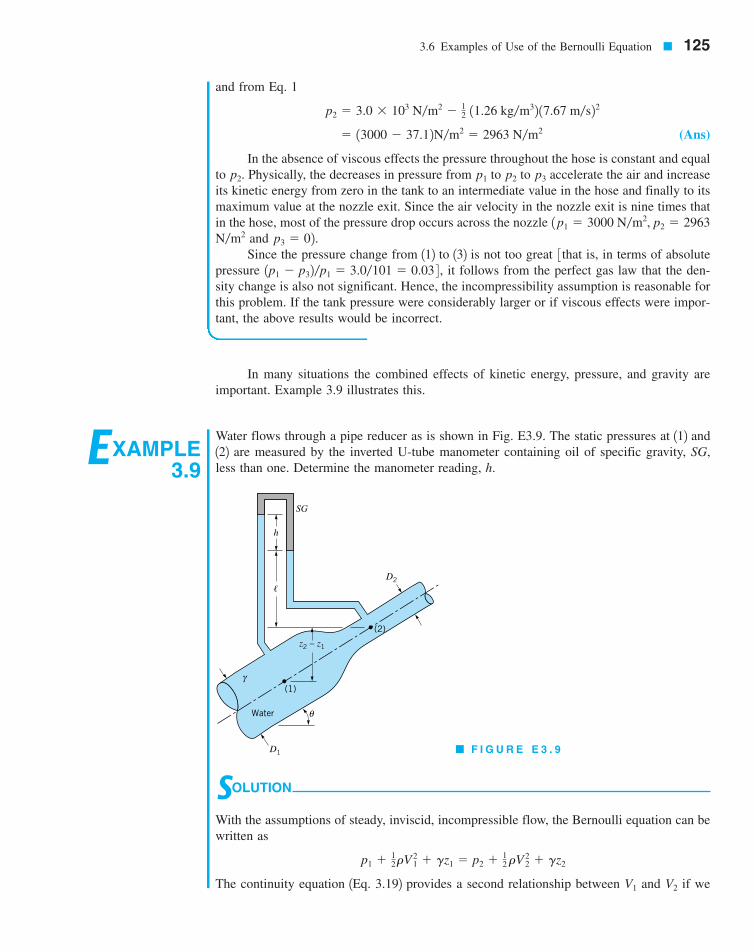
EXAMPLE3.9
Water flows through a pipe reducer as is shown in Fig. E3.9. The static pressures at 112 and122 are measured by the inverted U-tube manometer containing oil of specific gravity, SG,less than one. Determine the manometer reading, h.
SOLUTION
With the assumptions of steady, inviscid, incompressible flow, the Bernoulli equation can bewritten as
The continuity equation 1Eq. 3.192 provides a second relationship between and if weV2V1
p1 � 12rV
21 � gz1 � p2 � 1
2rV22 � gz2
� F I G U R E E 3 . 9
�
γ(1)
z2 – z1
(2)
Water θ
D1
D2
h
SG
7708d_c03_125 8/10/01 3:28 PM Page 125 mac120 mac120:1st shift:
126 � Chapter 3 / Elementary Fluid Dynamics—The Bernoulli Equation
In general, an increase in velocity is accompanied by a decrease in pressure. For ex-ample, the velocity of the air flowing over the top surface of an airplane wing is, on the av-erage, faster than that flowing under the bottom surface. Thus, the net pressure force is greateron the bottom than on the top—the wing generates a lift.
If the differences in velocity are considerable, the differences in pressure can also beconsiderable. For flows of gases, this may introduce compressibility effects as discussed inSection 3.8 and Chapter 11. For flows of liquids, this may result in cavitation, a potentiallydangerous situation that results when the liquid pressure is reduced to the vapor pressure andthe liquid “boils.”
As discussed in Chapter 1, the vapor pressure, pv, is the pressure at which vapor bub-bles form in a liquid. It is the pressure at which the liquid starts to boil. Obviously this pres-sure depends on the type of liquid and its temperature. For example, water, which boils at
at standard atmospheric pressure, 14.7 psia, boils at if the pressure is 0.507 psia.That is, psia at and psia at 1See Tables B.1 and B.2.2
One way to produce cavitation in a flowing liquid is noted from the Bernoulli equa-tion. If the fluid velocity is increased 1for example, by a reduction in flow area as shown inFig. 3.162 the pressure will decrease. This pressure decrease 1needed to accelerate the fluidthrough the constriction2 can be large enough so that the pressure in the liquid is reduced toits vapor pressure. A simple example of cavitation can be demonstrated with an ordinary gar-den hose. If the hose is “kinked,” a restriction in the flow area in some ways analogous to
212 °F.pv � 14.780 °Fpv � 0.50780 °F212 °F
assume the velocity profiles are uniform at those two locations and the fluid incompressible:
By combining these two equations we obtain
(1)
This pressure difference is measured by the manometer and can be determined by using thepressure-depth ideas developed in Chapter 2. Thus,
or
(2)
As discussed in Chapter 2, this pressure difference is neither merely nor Equations 1 and 2 can be combined to give the desired result as follows:
or since
(Ans)
The difference in elevation, was not needed because the change in elevationterm in the Bernoulli equation exactly cancels the elevation term in the manometer equation.However, the pressure difference, depends on the angle because of the elevation,
in Eq. 1. Thus, for a given flowrate, the pressure difference, as measuredby a pressure gage would vary with but the manometer reading, h, would be independentof u.
u,p1 � p2,z1 � z2,
u,p1 � p2,
z1 � z2,
h � 1Q�A222 1 � 1A2�A1222g11 � SG2
V2 � Q�A2
11 � SG2gh �1
2 rV 2
2 c1 � aA2
A1b2 d
g1h � z1 � z22.gh
p1 � p2 � g1z2 � z12 � 11 � SG2gh
p1 � g 1z2 � z12 � g/ � gh � SG gh � g/ � p2
p1 � p2 � g1z2 � z12 � 12rV
22 31 � 1A2�A122 4
Q � A1V1 � A2V2
V3.6 Venturi channel
Cavitation occurswhen the pressureis reduced to thevapor pressure.
7708d_c03_126 8/10/01 3:28 PM Page 126 mac120 mac120:1st shift:
3.6 Examples of Use of the Bernoulli Equation � 127
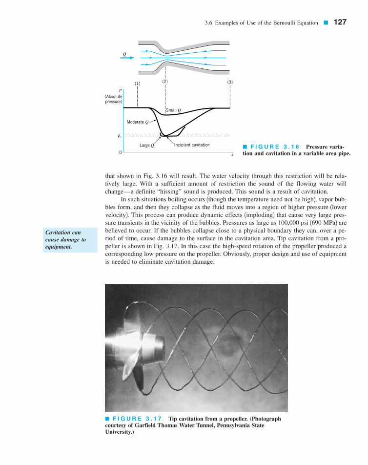
that shown in Fig. 3.16 will result. The water velocity through this restriction will be rela-tively large. With a sufficient amount of restriction the sound of the flowing water willchange—a definite “hissing” sound is produced. This sound is a result of cavitation.
In such situations boiling occurs 1though the temperature need not be high2, vapor bub-bles form, and then they collapse as the fluid moves into a region of higher pressure 1lowervelocity2. This process can produce dynamic effects 1imploding2 that cause very large pres-sure transients in the vicinity of the bubbles. Pressures as large as 100,000 psi 1690 MPa2 arebelieved to occur. If the bubbles collapse close to a physical boundary they can, over a pe-riod of time, cause damage to the surface in the cavitation area. Tip cavitation from a pro-peller is shown in Fig. 3.17. In this case the high-speed rotation of the propeller produced acorresponding low pressure on the propeller. Obviously, proper design and use of equipmentis needed to eliminate cavitation damage.
Q
p
(Absolutepressure)
(1) (2) (3)
Small Q
Moderate Q
Large Q Incipient cavitation
pv
0 x
� F I G U R E 3 . 1 6 Pressure varia-tion and cavitation in a variable area pipe.
� F I G U R E 3 . 1 7 Tip cavitation from a propeller. (Photographcourtesy of Garfield Thomas Water Tunnel, Pennsylvania State University.)
Cavitation cancause damage toequipment.
7708d_c03_127 8/13/01 1:40 AM Page 127
128 � Chapter 3 / Elementary Fluid Dynamics—The Bernoulli Equation
EXAMPLE3.10
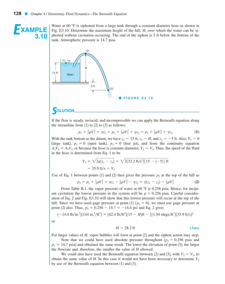
Water at is siphoned from a large tank through a constant diameter hose as shown inFig. E3.10. Determine the maximum height of the hill, H, over which the water can be si-phoned without cavitation occurring. The end of the siphon is 5 ft below the bottom of thetank. Atmospheric pressure is 14.7 psia.
60 °F
SOLUTION
If the flow is steady, inviscid, and incompressible we can apply the Bernoulli equation alongthe streamline from 112 to 122 to 132 as follows:
(1)
With the tank bottom as the datum, we have and Also,1large tank2, 1open tank2, 1free jet2, and from the continuity equationor because the hose is constant diameter, Thus, the speed of the fluid
in the hose is determined from Eq. 1 to be
Use of Eq. 1 between points 112 and 122 then gives the pressure at the top of the hill as
(2)
From Table B.1, the vapor pressure of water at is 0.256 psia. Hence, for incipi-ent cavitation the lowest pressure in the system will be psia. Careful consider-ation of Eq. 2 and Fig. E3.10 will show that this lowest pressure will occur at the top of thehill. Since we have used gage pressure at point 112 we must use gage pressure atpoint 122 also. Thus, psi and Eq. 2 gives
or
(Ans)
For larger values of H, vapor bubbles will form at point 122 and the siphon action may stop.Note that we could have used absolute pressure throughout 1 psia and
psia2 and obtained the same result. The lower the elevation of point 132, the largerthe flowrate and, therefore, the smaller the value of H allowed.
We could also have used the Bernoulli equation between 122 and 132, with toobtain the same value of H. In this case it would not have been necessary to determine by use of the Bernoulli equation between 112 and 132. V2
V2 � V3,
p1 � 14.7p2 � 0.256
H � 28.2 ft
1�14.4 lb�in.22 1144 in.2�ft22 � 162.4 lb�ft32 115 � H2ft � 12 11.94 slugs�ft32 135.9 ft�s22
p2 � 0.256 � 14.7 � �14.41p1 � 02,
p � 0.25660 °F
p2 � p1 � 12rV
21 � gz1 � 1
2rV22 � gz2 � g1z1 � z22 � 1
2rV22
p2
� 35.9 ft�s � V2
V3 � 22g1z1 � z32 � 22132.2 ft�s22 315 � 1�52 4 ft
V2 � V3.A2V2 � A3V3,p3 � 0p1 � 0
V1 � 0z3 � �5 ft.z1 � 15 ft, z2 � H,
p1 � 12rV
21 � gz1 � p2 � 1
2rV22 � gz2 � p3 � 1
2rV23 � gz3
Water
(1)
(2)
(3)5 ft
H
15 ft
� F I G U R E E 3 . 1 0
7708d_c03_100-159 7/5/01 8:27 AM Page 128
3.6.3 Flowrate Measurement
Many types of devices using principles involved in the Bernoulli equation have been devel-oped to measure fluid velocities and flowrates. The Pitot-static tube discussed in Section 3.5is an example. Other examples discussed below include devices to measure flowrates in pipesand conduits and devices to measure flowrates in open channels. In this chapter we will con-sider “ideal” flow meters—those devoid of viscous, compressibility, and other “real-world”effects. Corrections for these effects are discussed in Chapters 8 and 10. Our goal here is tounderstand the basic operating principles of these simple flow meters.
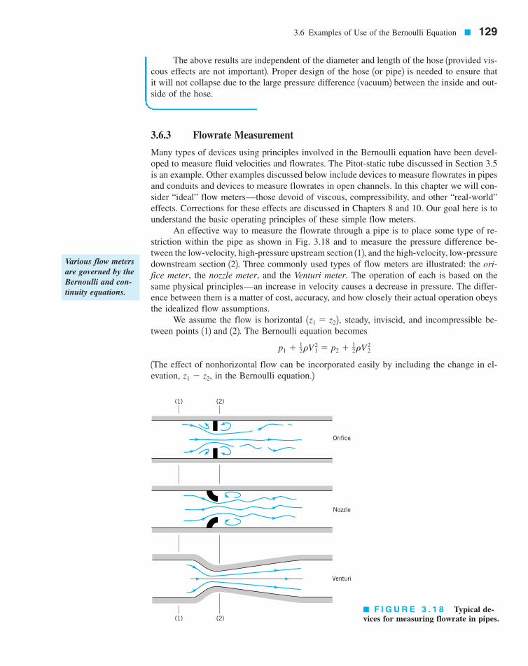
An effective way to measure the flowrate through a pipe is to place some type of re-striction within the pipe as shown in Fig. 3.18 and to measure the pressure difference be-tween the low-velocity, high-pressure upstream section 112, and the high-velocity, low-pressuredownstream section 122. Three commonly used types of flow meters are illustrated: the ori-fice meter, the nozzle meter, and the Venturi meter. The operation of each is based on thesame physical principles—an increase in velocity causes a decrease in pressure. The differ-ence between them is a matter of cost, accuracy, and how closely their actual operation obeysthe idealized flow assumptions.
We assume the flow is horizontal steady, inviscid, and incompressible be-tween points 112 and 122. The Bernoulli equation becomes
1The effect of nonhorizontal flow can be incorporated easily by including the change in el-evation, in the Bernoulli equation.2z1 � z2,
p1 � 12rV
21 � p2 � 1
2rV22
1z1 � z22,
3.6 Examples of Use of the Bernoulli Equation � 129
The above results are independent of the diameter and length of the hose 1provided vis-cous effects are not important2. Proper design of the hose 1or pipe2 is needed to ensure thatit will not collapse due to the large pressure difference 1vacuum2 between the inside and out-side of the hose.
� F I G U R E 3 . 1 8 Typical de-vices for measuring flowrate in pipes.
(1) (2)
(1) (2)
Venturi
Nozzle
Orifice
Various flow metersare governed by theBernoulli and con-tinuity equations.
7708d_c03_129 8/13/01 1:41 AM Page 129
If we assume the velocity profiles are uniform at sections 112 and 122, the continuityequation 1Eq. 3.192 can be written as
where is the small flow area at section 122. Combination of these two equa-tions results in the following theoretical flowrate
(3.20)
Thus, for a given flow geometry and the flowrate can be determined if the pressuredifference, is measured. The actual measured flowrate, will be smaller thanthis theoretical result because of various differences between the “real world” and the as-sumptions used in the derivation of Eq. 3.20. These differences 1which are quite consistentand may be as small as 1 to 2% or as large as 40%, depending on the geometry used2 arediscussed in Chapter 8.
Qactual,p1 � p2,A221A1
Q � A2 B 21p1 � p22
r 31 � 1A2�A122 4
1A2 6 A12A2
Q � A1V1 � A2V2
130 � Chapter 3 / Elementary Fluid Dynamics—The Bernoulli Equation
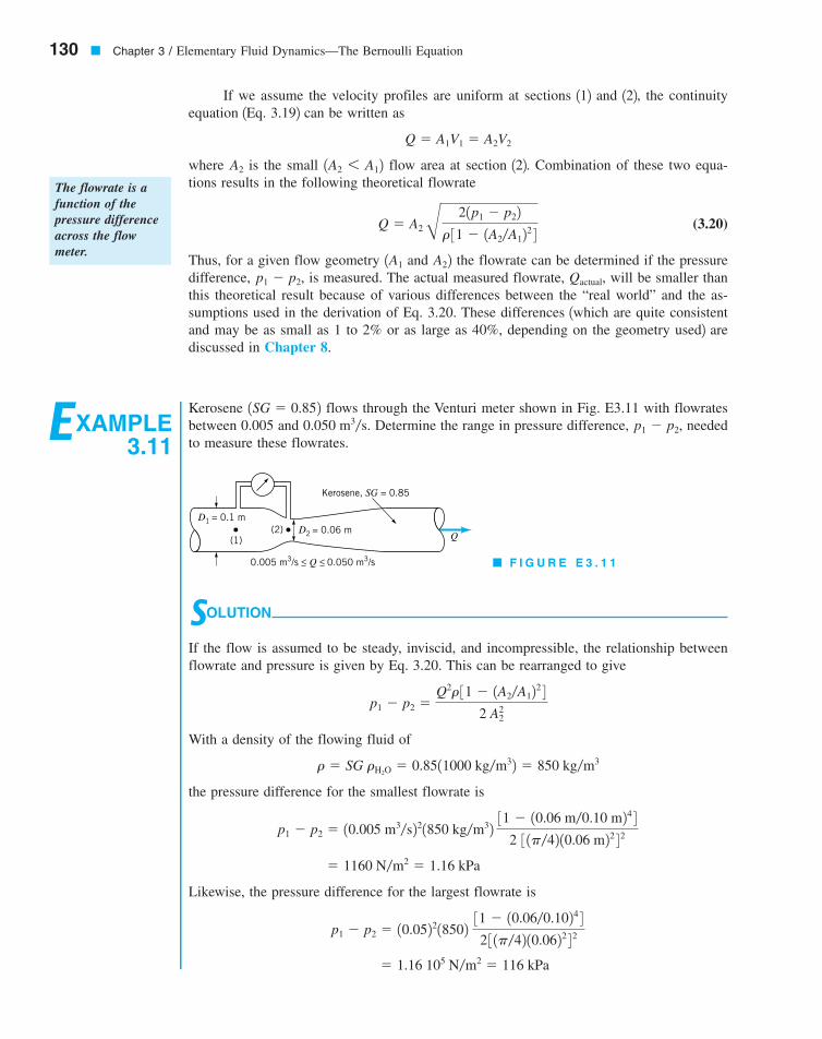
EXAMPLE3.11
Kerosene flows through the Venturi meter shown in Fig. E3.11 with flowratesbetween 0.005 and Determine the range in pressure difference, neededto measure these flowrates.
p1 � p2,0.050 m3�s.1SG � 0.852
D1 = 0.1 m
(1)(2)
0.005 m3/s < Q < 0.050 m3/s
D2 = 0.06 m
Kerosene, SG = 0.85
Q
SOLUTION
If the flow is assumed to be steady, inviscid, and incompressible, the relationship betweenflowrate and pressure is given by Eq. 3.20. This can be rearranged to give
With a density of the flowing fluid of
the pressure difference for the smallest flowrate is
Likewise, the pressure difference for the largest flowrate is
� 1.16 105 N�m2 � 116 kPa
p1 � p2 � 10.052218502 31 � 10.06�0.1024 4
2 3 1p�42 10.0622 4 2
� 1160 N�m2 � 1.16 kPa
p1 � p2 � 10.005 m3�s221850 kg�m32 31 � 10.06 m�0.10 m24 4
2 3 1p�42 10.06 m22 4 2
r � SG rH2O � 0.8511000 kg�m32 � 850 kg�m3
p1 � p2 �Q2r 31 � 1A2�A12
2 4
2 A22
� F I G U R E E 3 . 1 1
The flowrate is afunction of thepressure differenceacross the flow meter.
7708d_c03_130 8/13/01 1:41 AM Page 130
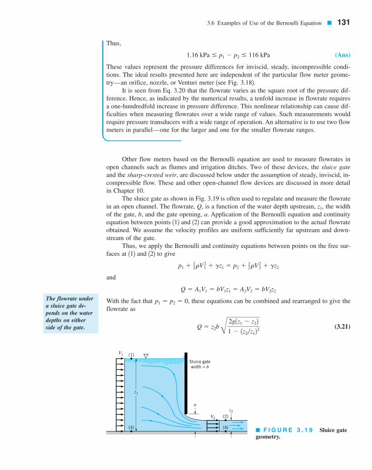
Other flow meters based on the Bernoulli equation are used to measure flowrates inopen channels such as flumes and irrigation ditches. Two of these devices, the sluice gateand the sharp-crested weir, are discussed below under the assumption of steady, inviscid, in-compressible flow. These and other open-channel flow devices are discussed in more detailin Chapter 10.
The sluice gate as shown in Fig. 3.19 is often used to regulate and measure the flowratein an open channel. The flowrate, Q, is a function of the water depth upstream, the widthof the gate, b, and the gate opening, a. Application of the Bernoulli equation and continuityequation between points 112 and 122 can provide a good approximation to the actual flowrateobtained. We assume the velocity profiles are uniform sufficiently far upstream and down-stream of the gate.
Thus, we apply the Bernoulli and continuity equations between points on the free sur-faces at 112 and 122 to give
and
With the fact that these equations can be combined and rearranged to give theflowrate as
(3.21)Q � z2b B 2g1z1 � z22
1 � 1z2�z122
p1 � p2 � 0,
Q � A1V1 � bV1z1 � A2V2 � bV2z2
p1 � 12rV
21 � gz1 � p2 � 1
2rV22 � gz2
z1,
3.6 Examples of Use of the Bernoulli Equation � 131
Thus,
(Ans)
These values represent the pressure differences for inviscid, steady, incompressible condi-tions. The ideal results presented here are independent of the particular flow meter geome-try—an orifice, nozzle, or Venturi meter 1see Fig. 3.182.
It is seen from Eq. 3.20 that the flowrate varies as the square root of the pressure dif-ference. Hence, as indicated by the numerical results, a tenfold increase in flowrate requiresa one-hundredfold increase in pressure difference. This nonlinear relationship can cause dif-ficulties when measuring flowrates over a wide range of values. Such measurements wouldrequire pressure transducers with a wide range of operation. An alternative is to use two flowmeters in parallel—one for the larger and one for the smaller flowrate ranges.
1.16 kPa � p1 � p2 � 116 kPa
The flowrate undera sluice gate de-pends on the waterdepths on eitherside of the gate.
� F I G U R E 3 . 1 9 Sluice gategeometry.
Sluice gatewidth = b
(1)
(2)
(4)(3)
V1
z1
a
V2
z2
7708d_c03_131 8/13/01 6:41 PM Page 131
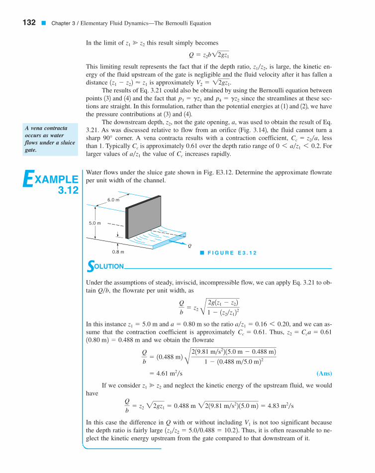
In the limit of this result simply becomes
This limiting result represents the fact that if the depth ratio, is large, the kinetic en-ergy of the fluid upstream of the gate is negligible and the fluid velocity after it has fallen adistance is approximately
The results of Eq. 3.21 could also be obtained by using the Bernoulli equation betweenpoints 132 and 142 and the fact that and since the streamlines at these sec-tions are straight. In this formulation, rather than the potential energies at 112 and 122, we havethe pressure contributions at 132 and 142.
The downstream depth, not the gate opening, a, was used to obtain the result of Eq.3.21. As was discussed relative to flow from an orifice 1Fig. 3.142, the fluid cannot turn asharp corner. A vena contracta results with a contraction coefficient, lessthan 1. Typically is approximately 0.61 over the depth ratio range of Forlarger values of the value of increases rapidly.Cca�z1
0 6 a�z1 6 0.2.Cc
Cc � z2�a,90°
z2,
p4 � gz2p3 � gz1
V2 � 12gz1.1z1 � z22 � z1
z1�z2,
Q � z2b12gz1
z1 � z2
132 � Chapter 3 / Elementary Fluid Dynamics—The Bernoulli Equation
EXAMPLE3.12
Water flows under the sluice gate shown in Fig. E3.12. Determine the approximate flowrateper unit width of the channel.
A vena contractaoccurs as waterflows under a sluicegate.
SOLUTION
Under the assumptions of steady, inviscid, incompressible flow, we can apply Eq. 3.21 to ob-tain the flowrate per unit width, as
In this instance m and so the ratio and we can as-sume that the contraction coefficient is approximately Thus,
and we obtain the flowrate
(Ans)
If we consider and neglect the kinetic energy of the upstream fluid, we wouldhave
In this case the difference in Q with or without including is not too significant becausethe depth ratio is fairly large Thus, it is often reasonable to ne-glect the kinetic energy upstream from the gate compared to that downstream of it.
1z1�z2 � 5.0�0.488 � 10.22.V1
Q
b� z2 22gz1 � 0.488 m 2219.81 m�s22 15.0 m2 � 4.83 m2�s
z1 � z2
� 4.61 m2�s
Q
b� 10.488 m2 B219.81 m�s22 15.0 m � 0.488 m2
1 � 10.488 m�5.0 m22
10.80 m2 � 0.488 mz2 � Cca � 0.61Cc � 0.61.
a�z1 � 0.16 6 0.20,a � 0.80 mz1 � 5.0
Q
b� z2 B 2g1z1 � z22
1 � 1z2�z122
Q�b,
Q
5.0 m
6.0 m
0.8 m � F I G U R E E 3 . 1 2
7708d_c03_132 8/13/01 6:41 PM Page 132
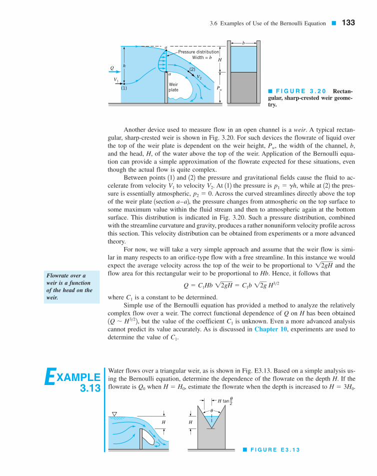
Another device used to measure flow in an open channel is a weir. A typical rectan-gular, sharp-crested weir is shown in Fig. 3.20. For such devices the flowrate of liquid overthe top of the weir plate is dependent on the weir height, the width of the channel, b,and the head, H, of the water above the top of the weir. Application of the Bernoulli equa-tion can provide a simple approximation of the flowrate expected for these situations, eventhough the actual flow is quite complex.
Between points 112 and 122 the pressure and gravitational fields cause the fluid to ac-celerate from velocity to velocity At 112 the pressure is while at 122 the pres-sure is essentially atmospheric, Across the curved streamlines directly above the topof the weir plate 1section a–a2, the pressure changes from atmospheric on the top surface tosome maximum value within the fluid stream and then to atmospheric again at the bottomsurface. This distribution is indicated in Fig. 3.20. Such a pressure distribution, combinedwith the streamline curvature and gravity, produces a rather nonuniform velocity profile acrossthis section. This velocity distribution can be obtained from experiments or a more advancedtheory.
For now, we will take a very simple approach and assume that the weir flow is simi-lar in many respects to an orifice-type flow with a free streamline. In this instance we wouldexpect the average velocity across the top of the weir to be proportional to and theflow area for this rectangular weir to be proportional to Hb. Hence, it follows that
where is a constant to be determined.Simple use of the Bernoulli equation has provided a method to analyze the relatively
complex flow over a weir. The correct functional dependence of Q on H has been obtainedbut the value of the coefficient is unknown. Even a more advanced analysis
cannot predict its value accurately. As is discussed in Chapter 10, experiments are used todetermine the value of C1.
C11Q � H3�22,
C1
Q � C1Hb 12gH � C1b 12g H3�2
12gH
p2 � 0.p1 � gh,V2.V1
Pw,
3.6 Examples of Use of the Bernoulli Equation � 133
Flowrate over aweir is a functionof the head on theweir.
Q
Pressure distributionWidth = b H
a
a
Weirplate(1)
V1
(2)
V2
Pw
h
b
� F I G U R E 3 . 2 0 Rectan-gular, sharp-crested weir geome-try.
EXAMPLE3.13
Water flows over a triangular weir, as is shown in Fig. E3.13. Based on a simple analysis us-ing the Bernoulli equation, determine the dependence of the flowrate on the depth H. If theflowrate is when estimate the flowrate when the depth is increased to H � 3H0.H � H0,Q0
H H
H tan _2θ
θ
� F I G U R E E 3 . 1 3
7708d_c03_133 8/13/01 1:46 AM Page 133
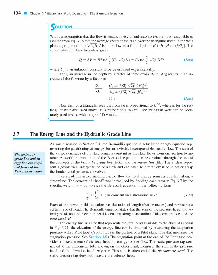
As was discussed in Section 3.4, the Bernoulli equation is actually an energy equation rep-resenting the partitioning of energy for an inviscid, incompressible, steady flow. The sum ofthe various energies of the fluid remains constant as the fluid flows from one section to an-other. A useful interpretation of the Bernoulli equation can be obtained through the use ofthe concepts of the hydraulic grade line 1HGL2 and the energy line 1EL2. These ideas repre-sent a geometrical interpretation of a flow and can often be effectively used to better graspthe fundamental processes involved.
For steady, inviscid, incompressible flow the total energy remains constant along astreamline. The concept of “head” was introduced by dividing each term in Eq. 3.7 by thespecific weight, to give the Bernoulli equation in the following form
(3.22)
Each of the terms in this equation has the units of length 1feet or meters2 and represents acertain type of head. The Bernoulli equation states that the sum of the pressure head, the ve-locity head, and the elevation head is constant along a streamline. This constant is called thetotal head, H.
The energy line is a line that represents the total head available to the fluid. As shownin Fig. 3.21, the elevation of the energy line can be obtained by measuring the stagnationpressure with a Pitot tube. 1A Pitot tube is the portion of a Pitot-static tube that measures thestagnation pressure. See Section 3.5.2 The stagnation point at the end of the Pitot tube pro-vides a measurement of the total head 1or energy2 of the flow. The static pressure tap con-nected to the piezometer tube shown, on the other hand, measures the sum of the pressurehead and the elevation head, This sum is often called the piezometric head. Thestatic pressure tap does not measure the velocity head.
p�g � z.
p
g�
V 2
2g� z � constant on a streamline � H
g � rg,
134 � Chapter 3 / Elementary Fluid Dynamics—The Bernoulli Equation
SOLUTION
With the assumption that the flow is steady, inviscid, and incompressible, it is reasonable toassume from Eq. 3.18 that the average speed of the fluid over the triangular notch in the weirplate is proportional to Also, the flow area for a depth of H is H Thecombination of these two ideas gives
(Ans)
where is an unknown constant to be determined experimentally.Thus, an increase in the depth by a factor of three 1from to 2 results in an in-
crease of the flowrate by a factor of
(Ans)
Note that for a triangular weir the flowrate is proportional to whereas for the rec-tangular weir discussed above, it is proportional to The triangular weir can be accu-rately used over a wide range of flowrates.
H3�2.H5�2,
� 15.6
Q3H0
QH0
�C2 tan1u�22 12g 13H02
5�2
C2 tan1u�22 12g 1H025�2
3H0H0
C2
Q � AV � H 2 tan u
2 1C2 12gH2 � C2 tan
u
2 12g H 5�2
3H tan 1u�22 4 .12gH.
3.7 The Energy Line and the Hydraulic Grade Line
The hydraulicgrade line and en-ergy line are graph-ical forms of theBernoulli equation.
7708d_c03_134 8/13/01 6:47 PM Page 134
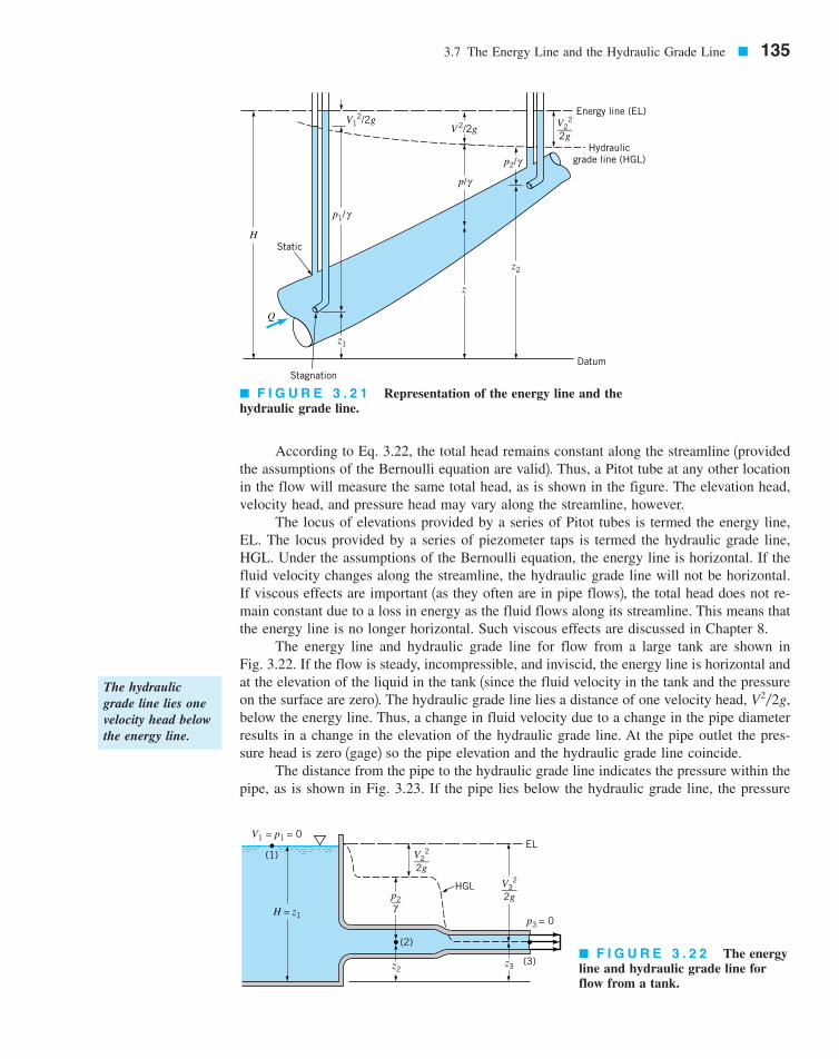
According to Eq. 3.22, the total head remains constant along the streamline 1providedthe assumptions of the Bernoulli equation are valid2. Thus, a Pitot tube at any other locationin the flow will measure the same total head, as is shown in the figure. The elevation head,velocity head, and pressure head may vary along the streamline, however.
The locus of elevations provided by a series of Pitot tubes is termed the energy line,EL. The locus provided by a series of piezometer taps is termed the hydraulic grade line,HGL. Under the assumptions of the Bernoulli equation, the energy line is horizontal. If thefluid velocity changes along the streamline, the hydraulic grade line will not be horizontal.If viscous effects are important 1as they often are in pipe flows2, the total head does not re-main constant due to a loss in energy as the fluid flows along its streamline. This means thatthe energy line is no longer horizontal. Such viscous effects are discussed in Chapter 8.
The energy line and hydraulic grade line for flow from a large tank are shown inFig. 3.22. If the flow is steady, incompressible, and inviscid, the energy line is horizontal andat the elevation of the liquid in the tank 1since the fluid velocity in the tank and the pressureon the surface are zero2. The hydraulic grade line lies a distance of one velocity head,below the energy line. Thus, a change in fluid velocity due to a change in the pipe diameterresults in a change in the elevation of the hydraulic grade line. At the pipe outlet the pres-sure head is zero 1gage2 so the pipe elevation and the hydraulic grade line coincide.
The distance from the pipe to the hydraulic grade line indicates the pressure within thepipe, as is shown in Fig. 3.23. If the pipe lies below the hydraulic grade line, the pressure
V2�2g,
3.7 The Energy Line and the Hydraulic Grade Line � 135
Q
HStatic
Stagnation
z1
p1/
V12/2g
V 2/2g
z
z2
p2/
V22
___2g
Hydraulicgrade line (HGL)
Energy line (EL)
Datum
p/ γ
γ
γ
HGL
EL
(3)
(2)
(1)
V1 = p1 = 0
H = z1
p2__
V22
___2g
z2z3
V32
___2g
p3 = 0
γ
� F I G U R E 3 . 2 1 Representation of the energy line and thehydraulic grade line.
� F I G U R E 3 . 2 2 The energyline and hydraulic grade line forflow from a tank.
The hydraulicgrade line lies onevelocity head belowthe energy line.
7708d_c03_135 8/13/01 1:46 AM Page 135
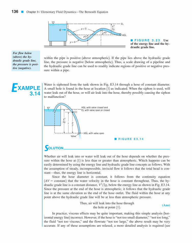
within the pipe is positive 1above atmospheric2. If the pipe lies above the hydraulic gradeline, the pressure is negative 1below atmospheric2. Thus, a scale drawing of a pipeline andthe hydraulic grade line can be used to readily indicate regions of positive or negative pres-sure within a pipe.
136 � Chapter 3 / Elementary Fluid Dynamics—The Bernoulli Equation
For flow below(above) the hy-draulic grade line,the pressure is posi-tive (negative).
Q
p > 0
p < 0
p/
zz
V2__2g
EL
HGLγp/γ
� F I G U R E 3 . 2 3 Useof the energy line and the hy-draulic grade line.
EXAMPLE3.14
Water is siphoned from the tank shown in Fig. E3.14 through a hose of constant diameter.A small hole is found in the hose at location 112 as indicated. When the siphon is used, willwater leak out of the hose, or will air leak into the hose, thereby possibly causing the siphonto malfunction?
ValveHGL with valve open
HGL with valve closed andEL with valve open or closed
(1)
V2__2g p_
γz
� F I G U R E E 3 . 1 4
SOLUTION
Whether air will leak into or water will leak out of the hose depends on whether the pres-sure within the hose at 112 is less than or greater than atmospheric. Which happens can beeasily determined by using the energy line and hydraulic grade line concepts as follows. Withthe assumption of steady, incompressible, inviscid flow it follows that the total head is con-stant—thus, the energy line is horizontal.
Since the hose diameter is constant, it follows from the continuity equationthat the water velocity in the hose is constant throughout. Thus, the hy-
draulic grade line is a constant distance, below the energy line as shown in Fig. E3.14.Since the pressure at the end of the hose is atmospheric, it follows that the hydraulic gradeline is at the same elevation as the end of the hose outlet. The fluid within the hose at anypoint above the hydraulic grade line will be at less than atmospheric pressure.
(Ans)
In practice, viscous effects may be quite important, making this simple analysis 1hor-izontal energy line2 incorrect. However, if the hose is “not too small diameter,” “not too long,”the fluid “not too viscous,” and the flowrate “not too large,” the above result may be veryaccurate. If any of these assumptions are relaxed, a more detailed analysis is required 1see
Thus, air will leak into the hose throughthe hole at point 112.
V 2�2g,1AV � constant2
7708d_c03_136 8/13/01 6:42 PM Page 136
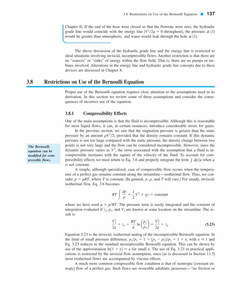
The above discussion of the hydraulic grade line and the energy line is restricted toideal situations involving inviscid, incompressible flows. Another restriction is that there areno “sources” or “sinks” of energy within the flow field. That is, there are no pumps or tur-bines involved. Alterations in the energy line and hydraulic grade line concepts due to thesedevices are discussed in Chapter 8.
3.8 Restrictions on Use of the Bernoulli Equation � 137
3.8 Restrictions on Use of the Bernoulli Equation
Proper use of the Bernoulli equation requires close attention to the assumptions used in itsderivation. In this section we review some of these assumptions and consider the conse-quences of incorrect use of the equation.
3.8.1 Compressibility Effects
One of the main assumptions is that the fluid is incompressible. Although this is reasonablefor most liquid flows, it can, in certain instances, introduce considerable errors for gases.
In the previous section, we saw that the stagnation pressure is greater than the staticpressure by an amount provided that the density remains constant. If this dynamicpressure is not too large compared with the static pressure, the density change between twopoints is not very large and the flow can be considered incompressible. However, since thedynamic pressure varies as the error associated with the assumption that a fluid is in-compressible increases with the square of the velocity of the fluid. To account for com-pressibility effects we must return to Eq. 3.6 and properly integrate the term when is not constant.
A simple, although specialized, case of compressible flow occurs when the tempera-ture of a perfect gas remains constant along the streamline—isothermal flow. Thus, we con-sider where T is constant. 1In general, p, and T will vary.2 For steady, inviscid,isothermal flow, Eq. 3.6 becomes
where we have used The pressure term is easily integrated and the constant ofintegration evaluated if and are known at some location on the streamline. The re-sult is
(3.23)
Equation 3.23 is the inviscid, isothermal analog of the incompressible Bernoulli equation. Inthe limit of small pressure difference, with andEq. 3.23 reduces to the standard incompressible Bernoulli equation. This can be shown byuse of the approximation for small The use of Eq. 3.23 in practical appli-cations is restricted by the inviscid flow assumption, since 1as is discussed in Section 11.52most isothermal flows are accompanied by viscous effects.
A much more common compressible flow condition is that of isentropic 1constant en-tropy2 flow of a perfect gas. Such flows are reversible adiabatic processes—“no friction or
e.ln11 � e2 � e
e � 1p1�p2 � 1 � 1p1 � p22�p2 � 1 � e,
V 21
2g� z1 �
RTg
ln ap1
p2b �
V 22
2g� z2
V1z1, p1,r � p�RT.
RT � dp
p�
1
2 V 2 � gz � constant
r,p � rRT,
r� dp�r
V 2,
rV 2�2,
The Bernoulliequation can bemodified for com-pressible flows.
Chapter 82. If the end of the hose were closed so that the flowrate were zero, the hydraulicgrade line would coincide with the energy line 1 throughout2, the pressure at 112would be greater than atmospheric, and water would leak through the hole at 112.V 2�2g � 0
7708d_c03_137 8/13/01 1:48 AM Page 137
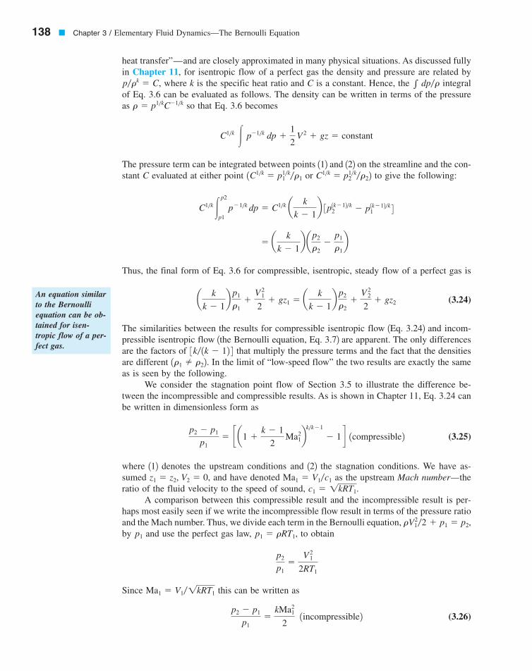
138 � Chapter 3 / Elementary Fluid Dynamics—The Bernoulli Equation
heat transfer”—and are closely approximated in many physical situations. As discussed fullyin Chapter 11, for isentropic flow of a perfect gas the density and pressure are related by
where k is the specific heat ratio and C is a constant. Hence, the integralof Eq. 3.6 can be evaluated as follows. The density can be written in terms of the pressureas so that Eq. 3.6 becomes
The pressure term can be integrated between points 112 and 122 on the streamline and the con-stant C evaluated at either point or to give the following:
Thus, the final form of Eq. 3.6 for compressible, isentropic, steady flow of a perfect gas is
(3.24)
The similarities between the results for compressible isentropic flow 1Eq. 3.242 and incom-pressible isentropic flow 1the Bernoulli equation, Eq. 3.72 are apparent. The only differencesare the factors of that multiply the pressure terms and the fact that the densitiesare different In the limit of “low-speed flow” the two results are exactly the sameas is seen by the following.
We consider the stagnation point flow of Section 3.5 to illustrate the difference be-tween the incompressible and compressible results. As is shown in Chapter 11, Eq. 3.24 canbe written in dimensionless form as
(3.25)
where 112 denotes the upstream conditions and 122 the stagnation conditions. We have as-sumed and have denoted as the upstream Mach number—theratio of the fluid velocity to the speed of sound,
A comparison between this compressible result and the incompressible result is per-haps most easily seen if we write the incompressible flow result in terms of the pressure ratioand the Mach number. Thus, we divide each term in the Bernoulli equation,by and use the perfect gas law, to obtain
Since this can be written as
(3.26)p2 � p1
p1�
kMa21
2 1incompressible2
Ma1 � V1�1kRT1
p2
p1�
V 21
2RT1
p1 � rRT1,p1
rV12�2 � p1 � p2,
c1 � 1kRT1.Ma1 � V1�c1z1 � z2, V2 � 0,
p2 � p1
p1� c a1 �
k � 1
2 Ma2
1bk�k�1
� 1 d 1compressible2
1r1 � r22.3k� 1k � 12 4
a k
k � 1b
p1
r1�
V 21
2� gz1 � a k
k � 1b
p2
r2�
V 22
2� gz2
� a k
k � 1b ap2
r2�
p1
r1b
C1�k�p2
p1 p
�1�k dp � C1�k a k
k � 1b 3p1k�12�k
2 � p1k�12�k1 4
C1�k � p21�k�r221C1�k � p1
1�k�r1
C1�k � p�1�k dp �1
2 V 2 � gz � constant
r � p1�kC�1�k
� dp�rp�rk � C,
An equation similarto the Bernoulliequation can be ob-tained for isen-tropic flow of a per-fect gas.
7708d_c03_100-159 8/13/01 1:52 AM Page 138
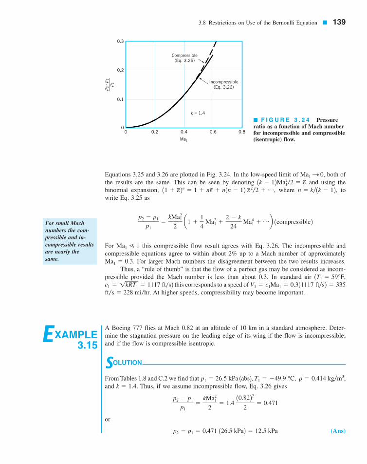
Equations 3.25 and 3.26 are plotted in Fig. 3.24. In the low-speed limit of both ofthe results are the same. This can be seen by denoting and using the binomial expansion, where towrite Eq. 3.25 as
For this compressible flow result agrees with Eq. 3.26. The incompressible andcompressible equations agree to within about 2% up to a Mach number of approximately
For larger Mach numbers the disagreement between the two results increases.Thus, a “rule of thumb” is that the flow of a perfect gas may be considered as incom-
pressible provided the Mach number is less than about 0.3. In standard air this corresponds to a speed of
At higher speeds, compressibility may become important.ft�s � 228 mi�hr.V1 � c1Ma1 � 0.311117 ft�s2 � 335c1 � 1kRT1 � 1117 ft�s2
1T1 � 59°F,
Ma1 � 0.3.
Ma1 � 1
p2 � p1
p1�
kMa21
2 a1 �
1
4 Ma2
1 �2 � k
24 Ma4
1 � pb 1compressible2
n � k� 1k � 12,11 � e~2n � 1 � ne~ � n1n � 12 e~2�2 � p,1k � 12Ma1
2�2 � e~Ma1 S 0,
3.8 Restrictions on Use of the Bernoulli Equation � 139
� F I G U R E 3 . 2 4 Pressureratio as a function of Mach numberfor incompressible and compressible(isentropic) flow.
For small Machnumbers the com-pressible and in-compressible resultsare nearly thesame.
Compressible(Eq. 3.25)
Incompressible(Eq. 3.26)
k = 1.4
0.3
0.2
0.1
00 0.2 0.4 0.6 0.8
Ma1
p 2 –
p1
____
__p 1
EXAMPLE3.15
A Boeing 777 flies at Mach 0.82 at an altitude of 10 km in a standard atmosphere. Deter-mine the stagnation pressure on the leading edge of its wing if the flow is incompressible;and if the flow is compressible isentropic.
SOLUTION
From Tables 1.8 and C.2 we find that 1abs2,and Thus, if we assume incompressible flow, Eq. 3.26 gives
or
(Ans)p2 � p1 � 0.471 126.5 kPa2 � 12.5 kPa
p2 � p1
p1�
kMa21
2� 1.4
10.82222
� 0.471
k � 1.4.r � 0.414 kg�m3,T1 � �49.9 °C,p1 � 26.5 kPa
7708d_c03_100-159 8/13/01 1:52 AM Page 139
3.8.2 Unsteady Effects
Another restriction of the Bernoulli equation 1Eq. 3.72 is the assumption that the flow issteady. For such flows, on a given streamline the velocity is a function of only s, the loca-tion along the streamline. That is, along a streamline For unsteady flows the ve-locity is also a function of time, so that along a streamline Thus whentaking the time derivative of the velocity to obtain the streamwise acceleration, we obtain
rather than just as is true for steady flow. For steadyflows the acceleration is due to the change in velocity resulting from a change in position ofthe particle 1the term2, whereas for unsteady flow there is an additional contributionto the acceleration resulting from a change in velocity with time at a fixed location 1the term2. These effects are discussed in detail in Chapter 4. The net effect is that the inclusionof the unsteady term, does not allow the equation of motion to be easily integrated1as was done to obtain the Bernoulli equation2 unless additional assumptions are made.
The Bernoulli equation was obtained by integrating the component of Newton’s sec-ond law 1Eq. 3.52 along the streamline. When integrated, the acceleration contribution to thisequation, the term, gave rise to the kinetic energy term in the Bernoulli equation. Ifthe steps leading to Eq. 3.5 are repeated with the inclusion of the unsteady effect the following is obtained:
For incompressible flow this can be easily integrated between points 112 and 122 to give
(3.27)
Equation 3.27 is an unsteady form of the Bernoulli equation valid for unsteady, incom-pressible, inviscid flow. Except for the integral involving the local acceleration, it isidentical to the steady Bernoulli equation. In general, it is not easy to evaluate this integralbecause the variation of along the streamline is not known. In some situations the con-cepts of “irrotational flow” and the “velocity potential” can be used to simplify this integral.These topics are discussed in Chapter 6.
0V�0t
0V�0t,
p1 �1
2 rV 2
1 � gz1 � r�s2
s1
0V
0t ds � p2 �
1
2 rV 2
2 � gz2 1along a streamline2
r 0V
0t ds � dp �
1
2 rd1V 22 � g dz � 0 1along a streamline2
10V�0t � 0212 rd1V 22
0V�0t,
0V�0tV 0V�0s
as � V 0V�0sas � 0V�0t � V 0V�0s
V � V1s, t2.V � V1s2.
140 � Chapter 3 / Elementary Fluid Dynamics—The Bernoulli Equation
On the other hand, if we assume isentropic flow, Eq. 3.25 gives
or
(Ans)
We see that at Mach 0.82 compressibility effects are of importance. The pressure 1and, to afirst approximation, the lift and drag on the airplane; see Chapter 92 is approximately
times greater according to the compressible flow calculations. This maybe very significant. As discussed in Chapter 11, for Mach numbers greater than 1 1super-sonic flow2 the differences between incompressible and compressible results are often notonly quantitative but also qualitative.
Note that if the airplane were flying at Mach 0.30 1rather than 0.822 the correspondingvalues would be for incompressible flow and forcompressible flow. The difference between these two results is about 2 percent.
p2 � p1 � 1.707 kPap2 � p1 � 1.670 kPa
14.7�12.5 � 1.18
p2 � p1 � 0.555 126.5 kPa2 � 14.7 kPa
p2 � p1
p1� e c1 �
11.4 � 122
10.8222 d 1.4�11.4�12� 1 f � 0.555
The Bernoulliequation can bemodified for un-steady flows.
7708d_c03_100-159 8/13/01 1:52 AM Page 140
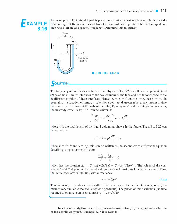
In a few unsteady flow cases, the flow can be made steady by an appropriate selectionof the coordinate system. Example 3.17 illustrates this.
3.8 Restrictions on Use of the Bernoulli Equation � 141
EXAMPLE3.16
An incompressible, inviscid liquid is placed in a vertical, constant-diameter U-tube as indi-cated in Fig. E3.16. When released from the nonequilibrium position shown, the liquid col-umn will oscillate at a specific frequency. Determine this frequency.
SOLUTION
The frequency of oscillation can be calculated by use of Eq. 3.27 as follows. Let points 112 and122 be at the air–water interfaces of the two columns of the tube and correspond to theequilibrium position of these interfaces. Hence, and if then Ingeneral, z is a function of time, For a constant diameter tube, at any instant in timethe fluid speed is constant throughout the tube, and the integral representingthe unsteady effect in Eq. 3.27 can be written as
where is the total length of the liquid column as shown in the figure. Thus, Eq. 3.27 canbe written as
Since and this can be written as the second-order differential equationdescribing simple harmonic motion
which has the solution The values of the con-stants and depend on the initial state 1velocity and position2 of the liquid at Thus,the liquid oscillates in the tube with a frequency
(Ans)
This frequency depends on the length of the column and the acceleration of gravity 1in amanner very similar to the oscillation of a pendulum2. The period of this oscillation 1the timerequired to complete an oscillation2 is t0 � 2p1/�2g.
v � 22g�/
t � 0.C2C1
z1t2 � C1 sin112g�/ t2 � C2 cos112g�/ t2.
d 2z
dt
2 �2g
/ z � 0
g � rg,V � dz�dt
g1�z2 � r/ dV
dt� gz
/
�s2
s1
0V
0t ds �
dV
dt �s2
s1
ds � / dV
dt
V1 � V2 � V,z � z1t2. z1 � �z.z2 � z,p1 � p2 � 0
z � 0
g
(1)
V1
(2)
V1
V2
�
z
z
Opentube
Equilibriumposition
= 0
� F I G U R E E 3 . 1 6
7708d_c03_100-159 8/13/01 1:52 AM Page 141
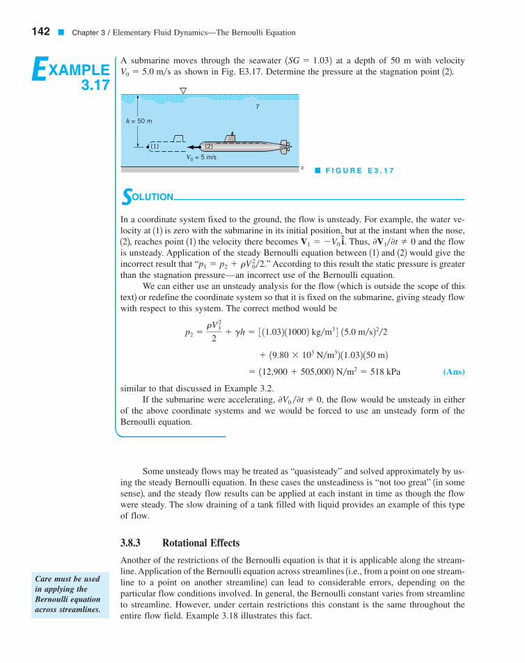
Some unsteady flows may be treated as “quasisteady” and solved approximately by us-ing the steady Bernoulli equation. In these cases the unsteadiness is “not too great” 1in somesense2, and the steady flow results can be applied at each instant in time as though the flowwere steady. The slow draining of a tank filled with liquid provides an example of this typeof flow.
3.8.3 Rotational Effects
Another of the restrictions of the Bernoulli equation is that it is applicable along the stream-line. Application of the Bernoulli equation across streamlines 1i.e., from a point on one stream-line to a point on another streamline2 can lead to considerable errors, depending on theparticular flow conditions involved. In general, the Bernoulli constant varies from streamlineto streamline. However, under certain restrictions this constant is the same throughout theentire flow field. Example 3.18 illustrates this fact.
142 � Chapter 3 / Elementary Fluid Dynamics—The Bernoulli Equation
Care must be usedin applying theBernoulli equationacross streamlines.
EXAMPLE3.17
A submarine moves through the seawater at a depth of 50 m with velocityas shown in Fig. E3.17. Determine the pressure at the stagnation point 122.V0 � 5.0 m�s
1SG � 1.032
SOLUTION
In a coordinate system fixed to the ground, the flow is unsteady. For example, the water ve-locity at 112 is zero with the submarine in its initial position, but at the instant when the nose,122, reaches point 112 the velocity there becomes Thus, and the flowis unsteady. Application of the steady Bernoulli equation between 112 and 122 would give theincorrect result that According to this result the static pressure is greaterthan the stagnation pressure—an incorrect use of the Bernoulli equation.
We can either use an unsteady analysis for the flow 1which is outside the scope of thistext2 or redefine the coordinate system so that it is fixed on the submarine, giving steady flowwith respect to this system. The correct method would be
(Ans)
similar to that discussed in Example 3.2.If the submarine were accelerating, the flow would be unsteady in either
of the above coordinate systems and we would be forced to use an unsteady form of theBernoulli equation.
0V0 �0t � 0,
� 112,900 � 505,0002 N�m2 � 518 kPa
� 19.80 � 103 N�m32 11.032 150 m2
p2 �rV 2
1
2� gh � 3 11.032 110002 kg�m3 4 15.0 m�s22�2
“p1 � p2 � rV 20�2.”
0V1�0t � 0V1 � �V0 i.
(1) (2)
h = 50 m
V0 = 5 m/s
x
γ
� F I G U R E E 3 . 1 7
7708d_c03_142 8/13/01 6:42 PM Page 142
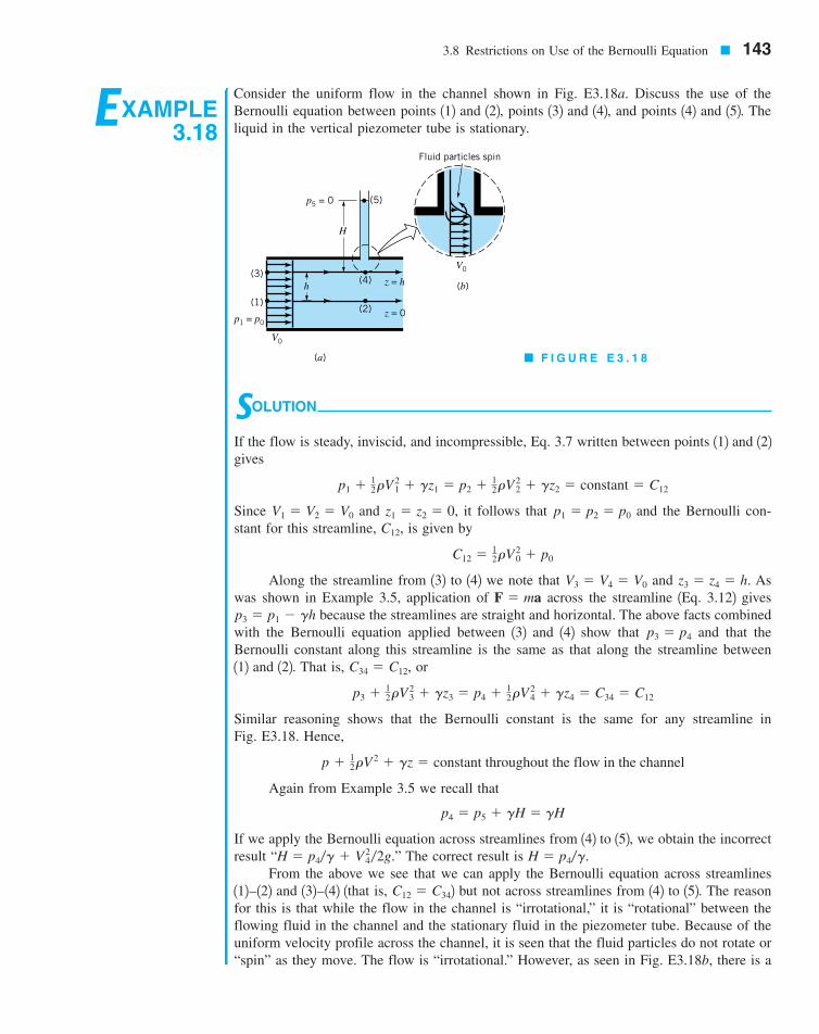
3.8 Restrictions on Use of the Bernoulli Equation � 143
EXAMPLE3.18
Consider the uniform flow in the channel shown in Fig. E3.18a. Discuss the use of theBernoulli equation between points 112 and 122, points 132 and 142, and points 142 and 152. Theliquid in the vertical piezometer tube is stationary.
(3)
(5)
(1)
(4)
(2)
V0
V0
p1 = p0
h
(a)
(b)z = h
z = 0
p5 = 0
H
Fluid particles spin
� F I G U R E E 3 . 1 8
SOLUTION
If the flow is steady, inviscid, and incompressible, Eq. 3.7 written between points 112 and 122gives
Since and it follows that and the Bernoulli con-stant for this streamline, is given by
Along the streamline from 132 to 142 we note that and Aswas shown in Example 3.5, application of across the streamline 1Eq. 3.122 gives
because the streamlines are straight and horizontal. The above facts combinedwith the Bernoulli equation applied between 132 and 142 show that and that theBernoulli constant along this streamline is the same as that along the streamline between112 and 122. That is, or
Similar reasoning shows that the Bernoulli constant is the same for any streamline inFig. E3.18. Hence,
Again from Example 3.5 we recall that
If we apply the Bernoulli equation across streamlines from 142 to 152, we obtain the incorrectresult The correct result is
From the above we see that we can apply the Bernoulli equation across streamlines112–122 and 132–142 1that is, 2 but not across streamlines from 142 to 152. The reasonfor this is that while the flow in the channel is “irrotational,” it is “rotational” between theflowing fluid in the channel and the stationary fluid in the piezometer tube. Because of theuniform velocity profile across the channel, it is seen that the fluid particles do not rotate or“spin” as they move. The flow is “irrotational.” However, as seen in Fig. E3.18b, there is a
C12 � C34
H � p4�g.“H � p4�g � V 24�2g.”
p4 � p5 � gH � gH
p � 12rV
2 � gz � constant throughout the flow in the channel
p3 � 12rV
23 � gz3 � p4 � 1
2rV24 � gz4 � C34 � C12
C34 � C12,
p3 � p4
p3 � p1 � ghF � ma
z3 � z4 � h.V3 � V4 � V0
C12 � 12rV
20 � p0
C12,p1 � p2 � p0z1 � z2 � 0,V1 � V2 � V0
p1 � 12rV
21 � gz1 � p2 � 1
2rV22 � gz2 � constant � C12
7708d_c03_100-159 8/13/01 1:52 AM Page 143
As is suggested by Example 3.18, if the flow is “irrotational” 1that is, the fluid parti-cles do not “spin” as they move2, it is appropriate to use the Bernoulli equation across stream-lines. However, if the flow is “rotational” 1fluid particles “spin”2, use of the Bernoulli equa-tion is restricted to flow along a streamline. The distinction between irrotational and rotationalflow is often a very subtle and confusing one. These topics are discussed in more detail inChapter 6. A thorough discussion can be found in more advanced texts 1Ref. 32.
3.8.4 Other Restrictions
Another restriction on the Bernoulli equation is that the flow is inviscid. As is discussed inSection 3.4, the Bernoulli equation is actually a first integral of Newton’s second law alonga streamline. This general integration was possible because, in the absence of viscous effects,the fluid system considered was a conservative system. The total energy of the system re-mains constant. If viscous effects are important the system is nonconservative and energylosses occur. A more detailed analysis is needed for these cases. Such material is presentedin Chapter 5.
The final basic restriction on use of the Bernoulli equation is that there are no me-chanical devices 1pumps or turbines2 in the system between the two points along the stream-line for which the equation is applied. These devices represent sources or sinks of energy.Since the Bernoulli equation is actually one form of the energy equation, it must be alteredto include pumps or turbines, if these are present. The inclusion of pumps and turbines iscovered in Chapters 5 and 12.
In this chapter we have spent considerable time investigating fluid dynamic situationsgoverned by a relatively simple analysis for steady, inviscid, incompressible flows. Manyflows can be adequately analyzed by use of these ideas. However, because of the rather se-vere restrictions imposed, many others cannot. An understanding of these basic ideas willprovide a firm foundation for the remainder of the topics in this book.
144 � Chapter 3 / Elementary Fluid Dynamics—The Bernoulli Equation
very thin shear layer between 142 and 152 in which adjacent fluid particles interact and rotateor “spin.” This produces a “rotational” flow. A more complete analysis would show that the Bernoulli equation cannot be applied across streamlines if the flow is “rotational” 1seeChapter 62.
The Bernoulliequation is notvalid for flows thatinvolve pumps orturbines.
In the E-book, click on any key wordor topic to go to that subject.Bernoulli equationCavitationContinuity equationEnergy lineF � ma normal to streamlineF � ma along streamline
Flowrate measurementFree jetHeadHydraulic grade lineMass flowrateNewton’s second lawNozzle meterOrifice meter
Pilot tubeStagnation pressureStatic pressureStreamlineVenturi meterVolume flowrateWeir
Key Words and Topics
1. Riley, W. F., and Sturges, L. D., Engineering Mechanics:Dynamics, 2nd Ed., Wiley, New York, 1996.2. Tipler, P. A., Physics, Worth, New York, 1982.
3. Panton, R. L., Incompressible Flow, Wiley, New York, 1984.
References
7708d_c03_144 8/13/01 6:42 PM Page 144
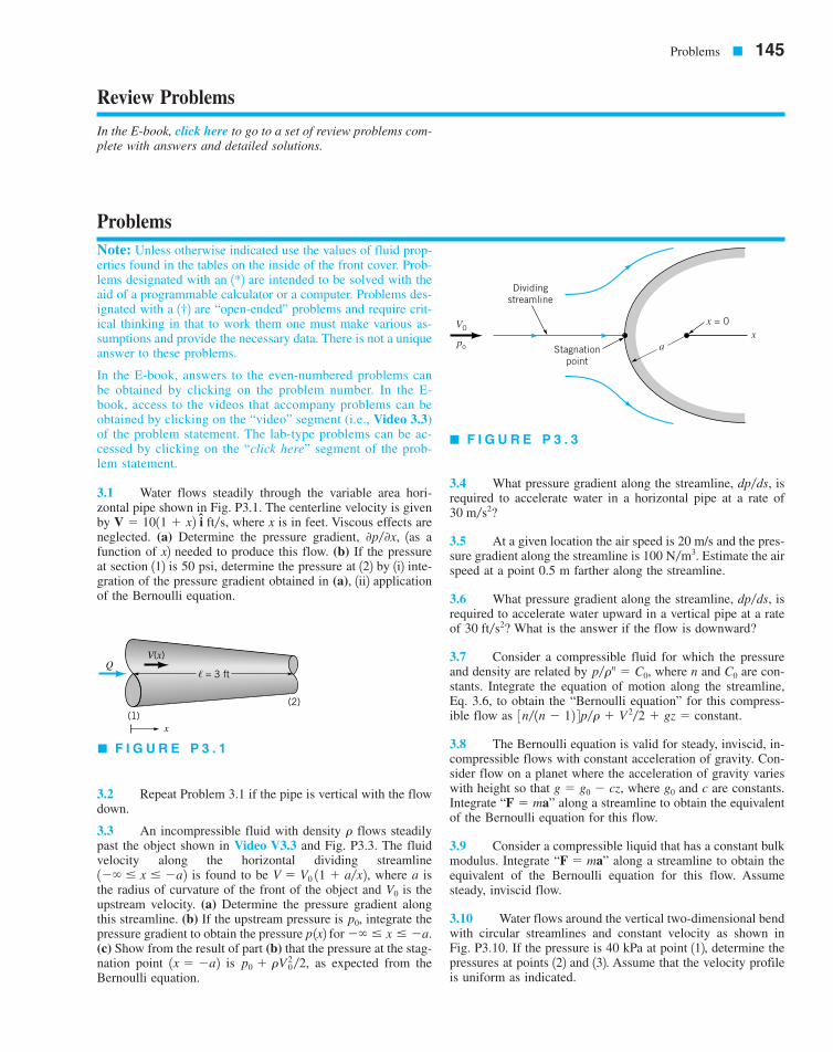
Problems � 145
In the E-book, click here to go to a set of review problems com-plete with answers and detailed solutions.
Review Problems
ProblemsNote: Unless otherwise indicated use the values of fluid prop-erties found in the tables on the inside of the front cover. Prob-lems designated with an 1*2 are intended to be solved with theaid of a programmable calculator or a computer. Problems des-ignated with a 1†2 are “open-ended” problems and require crit-ical thinking in that to work them one must make various as-sumptions and provide the necessary data. There is not a uniqueanswer to these problems.
In the E-book, answers to the even-numbered problems canbe obtained by clicking on the problem number. In the E-book, access to the videos that accompany problems can beobtained by clicking on the “video” segment (i.e., Video 3.3)of the problem statement. The lab-type problems can be ac-cessed by clicking on the “click here” segment of the prob-lem statement.
3.1 Water flows steadily through the variable area hori-zontal pipe shown in Fig. P3.1. The centerline velocity is givenby where x is in feet. Viscous effects areneglected. (a) Determine the pressure gradient, 1as afunction of x2 needed to produce this flow. (b) If the pressureat section 112 is 50 psi, determine the pressure at 122 by 1i2 inte-gration of the pressure gradient obtained in (a), 1ii2 applicationof the Bernoulli equation.
3.2 Repeat Problem 3.1 if the pipe is vertical with the flowdown.
3.3 An incompressible fluid with density flows steadilypast the object shown in Video V3.3 and Fig. P3.3. The fluidvelocity along the horizontal dividing streamline
is found to be where a isthe radius of curvature of the front of the object and is theupstream velocity. (a) Determine the pressure gradient alongthis streamline. (b) If the upstream pressure is integrate thepressure gradient to obtain the pressure p 1x2 for (c) Show from the result of part (b) that the pressure at the stag-nation point is as expected from theBernoulli equation.
3.4 What pressure gradient along the streamline, , isrequired to accelerate water in a horizontal pipe at a rate of
?
3.5 At a given location the air speed is 20 m/s and the pres-sure gradient along the streamline is Estimate the airspeed at a point 0.5 m farther along the streamline.
3.6 What pressure gradient along the streamline, , isrequired to accelerate water upward in a vertical pipe at a rateof What is the answer if the flow is downward?
3.7 Consider a compressible fluid for which the pressureand density are related by where n and are con-stants. Integrate the equation of motion along the streamline,Eq. 3.6, to obtain the “Bernoulli equation” for this compress-ible flow as
3.8 The Bernoulli equation is valid for steady, inviscid, in-compressible flows with constant acceleration of gravity. Con-sider flow on a planet where the acceleration of gravity varieswith height so that where and c are constants.Integrate along a streamline to obtain the equivalentof the Bernoulli equation for this flow.
3.9 Consider a compressible liquid that has a constant bulkmodulus. Integrate along a streamline to obtain theequivalent of the Bernoulli equation for this flow. Assumesteady, inviscid flow.
3.10 Water flows around the vertical two-dimensional bendwith circular streamlines and constant velocity as shown inFig. P3.10. If the pressure is 40 kPa at point 112, determine thepressures at points 122 and 132. Assume that the velocity profileis uniform as indicated.
“F � ma”
“F � ma”g0g � g0 � cz,
3n� 1n � 12 4p�r � V 2�2 � gz � constant.
C0p�rn � C0,
30 ft�s2?
dp�ds
100 N�m3.
30 m�s2
dp�ds
p0 � rV 20 �2,1x � �a2
� x �a.p0,
V0
V � V0 11 � a�x2,1� x �a2
r
0p�0x,V � 1011 � x2 i ft�s,
QV(x)
(1)(2)
� = 3 ft
x
� F I G U R E P 3 . 1
Dividingstreamline
Stagnationpoint
V0
po ax
x = 0
� F I G U R E P 3 . 3
7708d_c03_100-159 8/13/01 1:52 AM Page 145
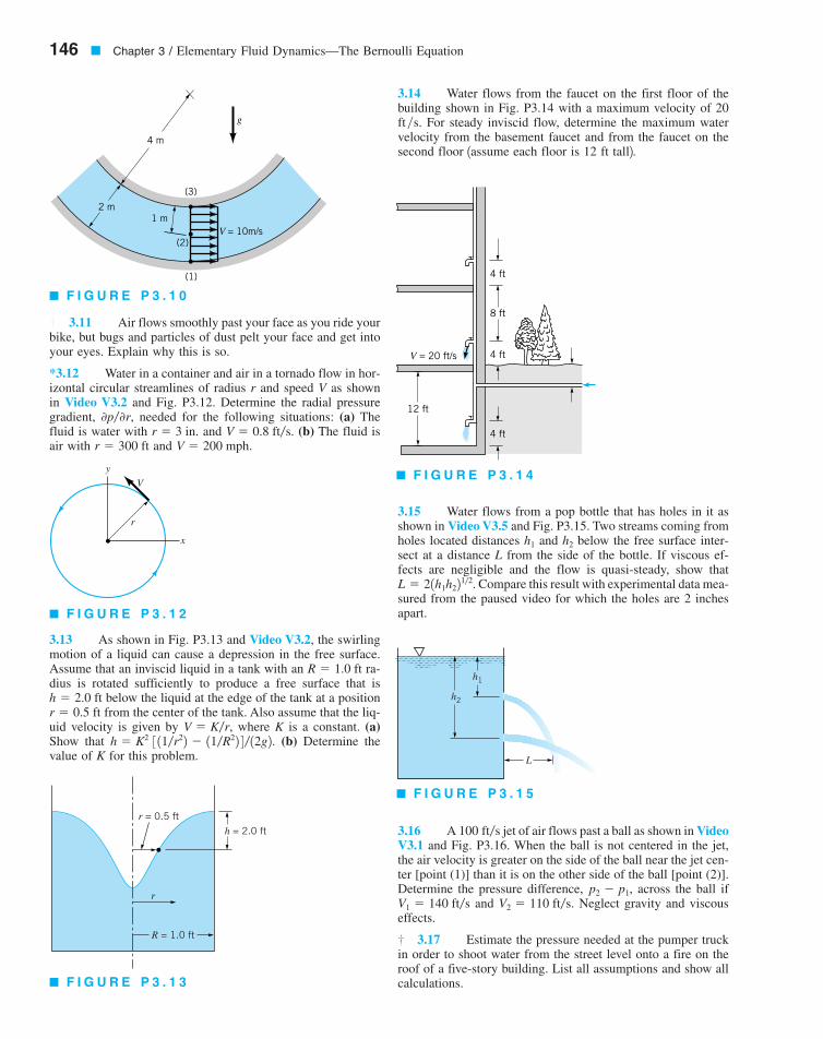
3.11 Air flows smoothly past your face as you ride yourbike, but bugs and particles of dust pelt your face and get intoyour eyes. Explain why this is so.
*3.12 Water in a container and air in a tornado flow in hor-izontal circular streamlines of radius r and speed V as shownin Video V3.2 and Fig. P3.12. Determine the radial pressuregradient, needed for the following situations: (a) Thefluid is water with and (b) The fluid isair with and
3.13 As shown in Fig. P3.13 and Video V3.2, the swirlingmotion of a liquid can cause a depression in the free surface.Assume that an inviscid liquid in a tank with an ra-dius is rotated sufficiently to produce a free surface that is
below the liquid at the edge of the tank at a positionfrom the center of the tank. Also assume that the liq-
uid velocity is given by where K is a constant. (a)Show that (b) Determine thevalue of K for this problem.
3.14 Water flows from the faucet on the first floor of thebuilding shown in Fig. P3.14 with a maximum velocity of 20ft�s. For steady inviscid flow, determine the maximum watervelocity from the basement faucet and from the faucet on thesecond floor 1assume each floor is 12 ft tall2.
3.15 Water flows from a pop bottle that has holes in it asshown in Video V3.5 and Fig. P3.15. Two streams coming fromholes located distances and below the free surface inter-sect at a distance L from the side of the bottle. If viscous ef-fects are negligible and the flow is quasi-steady, show that
Compare this result with experimental data mea-sured from the paused video for which the holes are 2 inchesapart.
3.16 A jet of air flows past a ball as shown in VideoV3.1 and Fig. P3.16. When the ball is not centered in the jet,the air velocity is greater on the side of the ball near the jet cen-ter [point (1)] than it is on the other side of the ball [point (2)].Determine the pressure difference, across the ball if
and Neglect gravity and viscouseffects.
3.17 Estimate the pressure needed at the pumper truckin order to shoot water from the street level onto a fire on theroof of a five-story building. List all assumptions and show allcalculations.
†
V2 � 110 ft�s.V1 � 140 ft�sp2 � p1,
100 ft�s
L � 21h1h221�2.
h2h1
h � K2 3 11�r22 � 11�R22 4 � 12g2.V � K�r,
r � 0.5 fth � 2.0 ft
R � 1.0 ft
V � 200 mph.r � 300 ftV � 0.8 ft�s.r � 3 in.
0p�0r,
†
146 � Chapter 3 / Elementary Fluid Dynamics—The Bernoulli Equation
(1)
(2)
(3)
1 m2 m
4 m
g
V = 10m/s
� F I G U R E P 3 . 1 0
y
x
r
V
� F I G U R E P 3 . 1 2
r = 0.5 ft
h = 2.0 ft
r
R = 1.0 ft
� F I G U R E P 3 . 1 3
V = 20 ft/s
12 ft
4 ft
4 ft
4 ft
8 ft
� F I G U R E P 3 . 1 4
L
h2
h1
� F I G U R E P 3 . 1 5
7708d_c03_146 8/13/01 6:43 PM Page 146

Problems � 147
3.18 A fire hose nozzle has a diameter of in. Accordingto some fire codes, the nozzle must be capable of delivering atleast 250 gal�min. If the nozzle is attached to a 3-in.-diameterhose, what pressure must be maintained just upstream of thenozzle to deliver this flowrate?
3.19 Water flowing from the 0.75-in.-diameter outlet shownin Video V8.6 and Fig. P3.19 rises 2.8 inches above the outlet.Determine the flowrate.
3.20 Pop (with the same properties as water) flows from a 4-in. diameter pop container that contains three holes as shown inFig. P3.20 (see Video 3.5). The diameter of each fluid stream is0.15 in., and the distance between holes is 2 in. If viscous effectsare negligible and quasi-steady conditions are assumed, determinethe time at which the pop stops draining from the top hole. Assume the pop surface is 2 in. above the top hole when Compare your results with the time you measure from the video.
*3.21 Water flowing from a pipe or a tank is acted upon bygravity and follows a curved trajectory as shown in Fig. P3.21and Videos V3.5 and V4.3. A simple flow meter can be con-structed as shown in Fig. P3.21. A point gage mounted a dis-tance L from the end of the horizontal pipe is adjusted to indi-cate that the top of the water stream is a distance x below theoutlet of the pipe. Show that the flowrate from this pipe of di-ameter D is given by
3.22 A person holds her hand out of an open car windowwhile the car drives through still air at 65 mph. Under standardatmospheric conditions, what is the maximum pressure on her
hand? What would be the maximum pressure if the “car” werean Indy 500 racer traveling 220 mph?
3.23 A differential pressure gage attached to a Pitot-statictube (see Video V3.4) is calibrated to give speed rather than thedifference between the stagnation and static pressures. The cal-ibration is done so that the speed indicated on the gage is theactual fluid speed if the fluid flowing past the Pitot-static tubeis air at standard sea level conditions. Assume the same deviceis used in water and the gage indicates a speed of 200 knots.Determine the water speed.
3.24 A 40-mph wind blowing past your house speeds up asit flows up and over the roof. If elevation effects are negligible,determine (a) the pressure at the point on the roof where thespeed is 60 mph if the pressure in the free stream blowing to-ward your house is 14.7 psia. Would this effect tend to push theroof down against the house, or would it tend to lift the roof?(b) Determine the pressure on a window facing the wind if thewindow is assumed to be a stagnation point.
3.25 Water flows steadily downward through the pipeshown in Fig. P3.25. Viscous effects are negligible, and the pres-sure gage indicates the pressure is zero at point (1). Determinethe flowrate and the pressure at point (2).
3.26 Small-diameter, high-pressure liquid jets can be usedto cut various materials as shown in Fig. P3.26. If viscous ef-fects are negligible, estimate the pressure needed to produce a0.10-mm-diameter water jet with a speed of 700 m�s. Deter-mine the flowrate.
Q � pD2L g1�2� 125�2 x1�22.
t � 0.
118
V2 = 110 ft/s
V1 = 140 ft/s
V = 100 ft/s
(2) (1)
� F I G U R E P 3 . 1 6
Q
2.8 in.
0.75 in.
� F I G U R E P 3 . 1 9
Surface at t = 0
2 in. 0.15 in.
2 in.
4 in.
2 in.
� F I G U R E P 3 . 2 0
L
Q
x
� F I G U R E P 3 . 2 1
7708d_c03_100-159 7/5/01 8:27 AM Page 147
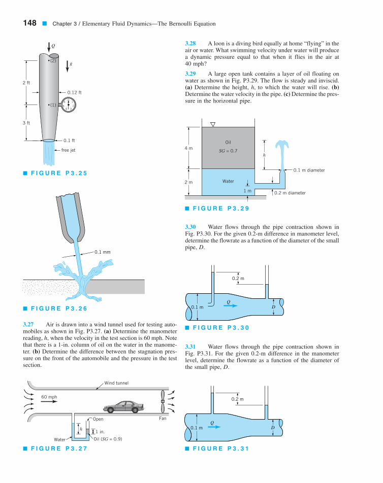
148 � Chapter 3 / Elementary Fluid Dynamics—The Bernoulli Equation
3.27 Air is drawn into a wind tunnel used for testing auto-mobiles as shown in Fig. P3.27. (a) Determine the manometerreading, h, when the velocity in the test section is 60 mph. Notethat there is a 1-in. column of oil on the water in the manome-ter. (b) Determine the difference between the stagnation pres-sure on the front of the automobile and the pressure in the testsection.
3.28 A loon is a diving bird equally at home “flying” in theair or water. What swimming velocity under water will producea dynamic pressure equal to that when it flies in the air at40 mph?
3.29 A large open tank contains a layer of oil floating onwater as shown in Fig. P3.29. The flow is steady and inviscid.(a) Determine the height, h, to which the water will rise. (b)Determine the water velocity in the pipe. (c) Determine the pres-sure in the horizontal pipe.
3.30 Water flows through the pipe contraction shown inFig. P3.30. For the given 0.2-m difference in manometer level,determine the flowrate as a function of the diameter of the smallpipe, D.
3.31 Water flows through the pipe contraction shown inFig. P3.31. For the given 0.2-m difference in the manometerlevel, determine the flowrate as a function of the diameter ofthe small pipe, D.
0.12 ft
0.1 ft
free jet
2 ft
0.12 ft
3 ft
0
234
16
5
(2)
(1)
Q
g
� F I G U R E P 3 . 2 5
0.1 mm
� F I G U R E P 3 . 2 6
Oil
SG = 0.7h
Water
0.1 m diameter
0.2 m diameter1 m
2 m
4 m
� F I G U R E P 3 . 2 9
Wind tunnel
Fan
60 mph
h
Water
Open
1 in.
Oil (SG = 0.9)
� F I G U R E P 3 . 2 7
0.2 m
Q0.1 m D
� F I G U R E P 3 . 3 0
0.2 m
Q0.1 m D
� F I G U R E P 3 . 3 1
7708d_c03_100-159 8/13/01 1:52 AM Page 148
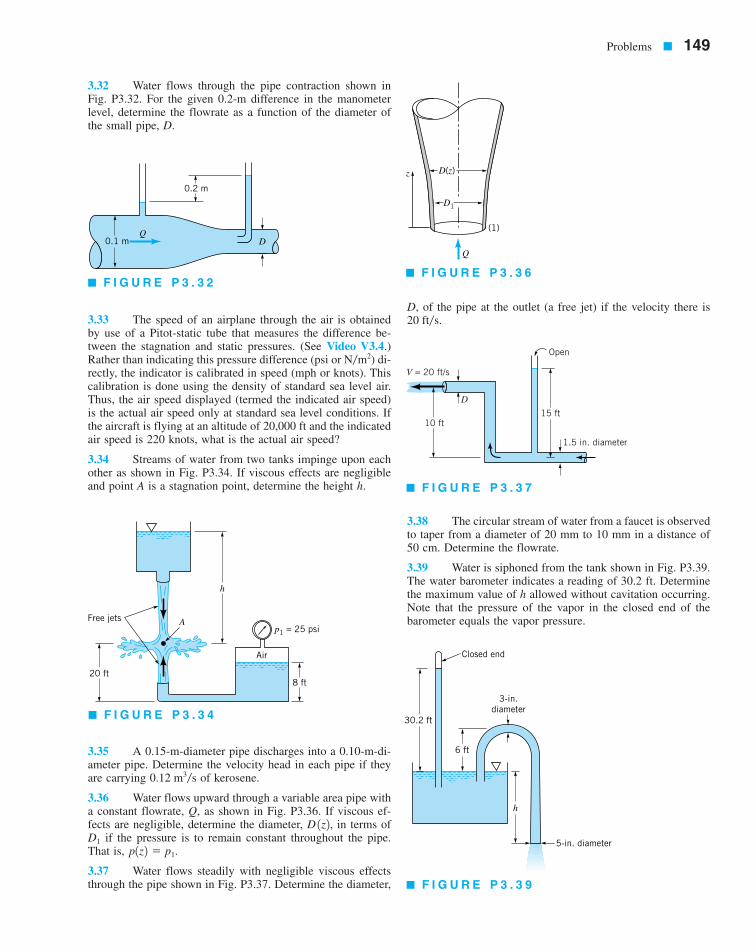
Problems � 149
3.32 Water flows through the pipe contraction shown inFig. P3.32. For the given 0.2-m difference in the manometerlevel, determine the flowrate as a function of the diameter ofthe small pipe, D.
3.33 The speed of an airplane through the air is obtainedby use of a Pitot-static tube that measures the difference be-tween the stagnation and static pressures. (See Video V3.4.)Rather than indicating this pressure difference (psi or ) di-rectly, the indicator is calibrated in speed (mph or knots). Thiscalibration is done using the density of standard sea level air.Thus, the air speed displayed (termed the indicated air speed)is the actual air speed only at standard sea level conditions. Ifthe aircraft is flying at an altitude of 20,000 ft and the indicatedair speed is 220 knots, what is the actual air speed?
3.34 Streams of water from two tanks impinge upon eachother as shown in Fig. P3.34. If viscous effects are negligibleand point A is a stagnation point, determine the height h.
3.35 A 0.15-m-diameter pipe discharges into a 0.10-m-di-ameter pipe. Determine the velocity head in each pipe if theyare carrying of kerosene.
3.36 Water flows upward through a variable area pipe witha constant flowrate, Q, as shown in Fig. P3.36. If viscous ef-fects are negligible, determine the diameter, in terms of
if the pressure is to remain constant throughout the pipe.That is,
3.37 Water flows steadily with negligible viscous effectsthrough the pipe shown in Fig. P3.37. Determine the diameter,
D, of the pipe at the outlet (a free jet) if the velocity there is
3.38 The circular stream of water from a faucet is observedto taper from a diameter of 20 mm to 10 mm in a distance of50 cm. Determine the flowrate.
3.39 Water is siphoned from the tank shown in Fig. P3.39.The water barometer indicates a reading of 30.2 ft. Determinethe maximum value of h allowed without cavitation occurring.Note that the pressure of the vapor in the closed end of thebarometer equals the vapor pressure.
20 ft�s.
p1z2 � p1.D1
D 1z2,
0.12 m3�s
N�m2
Q0.1 m
0.2 m
D
� F I G U R E P 3 . 3 2
Air
p1 = 25 psi
8 ft20 ft
Free jets A
h
� F I G U R E P 3 . 3 4
D1
D(z)z
Q
(1)
� F I G U R E P 3 . 3 6
V = 20 ft/s
D
10 ft15 ft
Open
1.5 in. diameter
� F I G U R E P 3 . 3 7
30.2 ft
6 ft
3-in.diameter
h
Closed end
5-in. diameter
� F I G U R E P 3 . 3 9
7708d_c03_100-159 7/5/01 8:27 AM Page 149
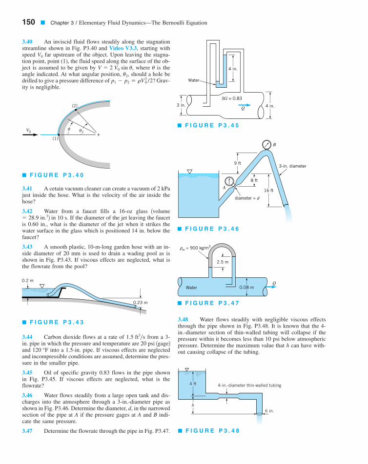
150 � Chapter 3 / Elementary Fluid Dynamics—The Bernoulli Equation
3.40 An inviscid fluid flows steadily along the stagnationstreamline shown in Fig. P3.40 and Video V3.3, starting withspeed far upstream of the object. Upon leaving the stagna-tion point, point (1), the fluid speed along the surface of the ob-ject is assumed to be given by where is theangle indicated. At what angular position, should a hole bedrilled to give a pressure difference of Grav-ity is negligible.
3.41 A cetain vacuum cleaner can create a vacuum of 2 kPajust inside the hose. What is the velocity of the air inside thehose?
3.42 Water from a faucet fills a 16-oz glass 1volume2 in 10 s. If the diameter of the jet leaving the faucet
is 0.60 in., what is the diameter of the jet when it strikes thewater surface in the glass which is positioned 14 in. below thefaucet?
3.43 A smooth plastic, 10-m-long garden hose with an in-side diameter of 20 mm is used to drain a wading pool as isshown in Fig. P3.43. If viscous effects are neglected, what isthe flowrate from the pool?
3.44 Carbon dioxide flows at a rate of from a 3-in. pipe in which the pressure and temperature are 20 psi 1gage2and into a 1.5-in. pipe. If viscous effects are neglectedand incompressible conditions are assumed, determine the pres-sure in the smaller pipe.
3.45 Oil of specific gravity 0.83 flows in the pipe shownin Fig. P3.45. If viscous effects are neglected, what is theflowrate?
3.46 Water flows steadily from a large open tank and dis-charges into the atmosphere through a 3-in.-diameter pipe asshown in Fig. P3.46. Determine the diameter, d, in the narrowedsection of the pipe at A if the pressure gages at A and B indi-cate the same pressure.
3.47 Determine the flowrate through the pipe in Fig. P3.47.
3.48 Water flows steadily with negligible viscous effectsthrough the pipe shown in Fig. P3.48. It is known that the 4-in.-diameter section of thin-walled tubing will collapse if thepressure within it becomes less than 10 psi below atmosphericpressure. Determine the maximum value that h can have with-out causing collapse of the tubing.120 °F
1.5 ft3�s
� 28.9 in.3
p1 � p2 � rV 20 /2?
u2,uV � 2 V0 sin u,
V0
θ θ2
(2)
(1)
V0
� F I G U R E P 3 . 4 0
9 ft
8 ft
3-in. diameter
diameter = d
16 ftA
B
� F I G U R E P 3 . 4 6
0.2 m
0.23 m
� F I G U R E P 3 . 4 3
Q
2.5 m
0.08 mWater
m = 900 kg/m3ρ
� F I G U R E P 3 . 4 7
4-in.-diameter thin-walled tubing
6 in.h
4 ft
� F I G U R E P 3 . 4 8
Water
SG = 0.83
Q3 in. 4 in.
4 in.
� F I G U R E P 3 . 4 5
7708d_c03_150 8/14/01 8:54 AM Page 150
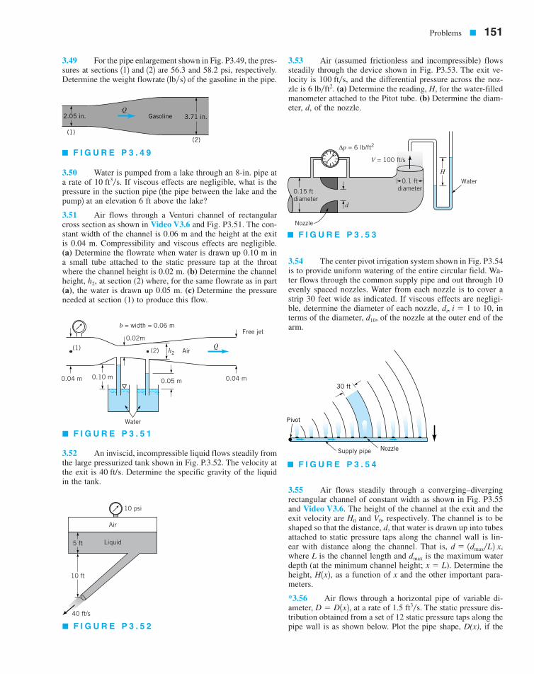
Problems � 151
3.49 For the pipe enlargement shown in Fig. P3.49, the pres-sures at sections 112 and 122 are 56.3 and 58.2 psi, respectively.Determine the weight flowrate 1lb�s2 of the gasoline in the pipe.
3.50 Water is pumped from a lake through an 8-in. pipe ata rate of If viscous effects are negligible, what is thepressure in the suction pipe 1the pipe between the lake and thepump2 at an elevation 6 ft above the lake?
3.51 Air flows through a Venturi channel of rectangularcross section as shown in Video V3.6 and Fig. P3.51. The con-stant width of the channel is 0.06 m and the height at the exitis 0.04 m. Compressibility and viscous effects are negligible.(a) Determine the flowrate when water is drawn up 0.10 m ina small tube attached to the static pressure tap at the throatwhere the channel height is 0.02 m. (b) Determine the channelheight, at section (2) where, for the same flowrate as in part(a), the water is drawn up 0.05 m. (c) Determine the pressureneeded at section (1) to produce this flow.
3.52 An inviscid, incompressible liquid flows steadily fromthe large pressurized tank shown in Fig. P.3.52. The velocity atthe exit is Determine the specific gravity of the liquidin the tank.
3.53 Air (assumed frictionless and incompressible) flowssteadily through the device shown in Fig. P3.53. The exit ve-locity is and the differential pressure across the noz-zle is (a) Determine the reading, H, for the water-filledmanometer attached to the Pitot tube. (b) Determine the diam-eter, d, of the nozzle.
3.54 The center pivot irrigation system shown in Fig. P3.54is to provide uniform watering of the entire circular field. Wa-ter flows through the common supply pipe and out through 10evenly spaced nozzles. Water from each nozzle is to cover astrip 30 feet wide as indicated. If viscous effects are negligi-ble, determine the diameter of each nozzle, to 10, interms of the diameter, of the nozzle at the outer end of thearm.
3.55 Air flows steadily through a converging–diverging rectangular channel of constant width as shown in Fig. P3.55and Video V3.6. The height of the channel at the exit and theexit velocity are and respectively. The channel is to beshaped so that the distance, d, that water is drawn up into tubesattached to static pressure taps along the channel wall is lin-ear with distance along the channel. That is,where L is the channel length and is the maximum waterdepth (at the minimum channel height; ). Determine theheight, as a function of x and the other important para-meters.
*3.56 Air flows through a horizontal pipe of variable di-ameter, at a rate of The static pressure dis-tribution obtained from a set of 12 static pressure taps along thepipe wall is as shown below. Plot the pipe shape, D(x), if the
1.5 ft3�s.D � D1x2,
H1x2, x � Ldmax
d � 1dmax�L2 x,
V0,H0
d10,di, i � 1
6 lb�ft2.100 ft�s,
40 ft/s.
h2,
10 ft3�s.
QGasoline 3.71 in.2.05 in.
(1)(2)
� F I G U R E P 3 . 4 9
QAir
0.02m
0.04 m 0.10 m
Water
0.05 m 0.04 m
(2)(1)
b = width = 0.06 m
h2
Free jet
� F I G U R E P 3 . 5 1
40 ft/s
10 ft
5 ft
10 psi
Liquid
Air
� F I G U R E P 3 . 5 2
∆p = 6 lb/ft2
d
0.15 ftdiameter
0.1 ftdiameter
Water
Nozzle
V = 100 ft/s
H
� F I G U R E P 3 . 5 3
Supply pipe Nozzle
30 ft
Pivot
� F I G U R E P 3 . 5 4
7708d_c03_100-159 8/13/01 1:52 AM Page 151
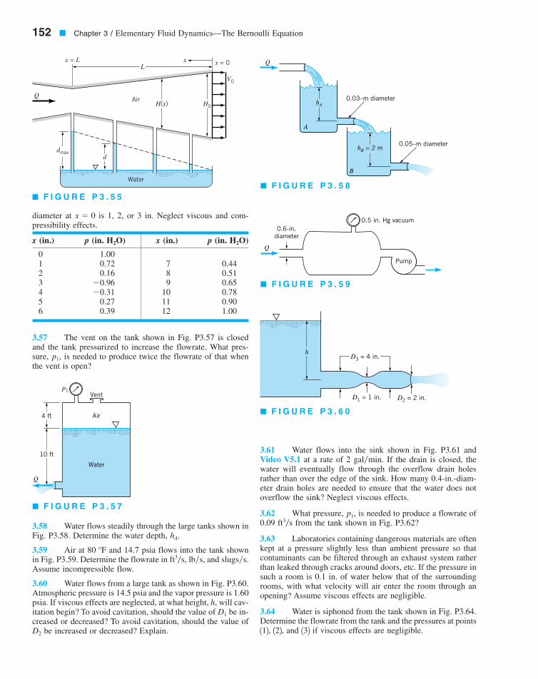
152 � Chapter 3 / Elementary Fluid Dynamics—The Bernoulli Equation
diameter at is 1, 2, or 3 in. Neglect viscous and com-pressibility effects.
3.57 The vent on the tank shown in Fig. P3.57 is closedand the tank pressurized to increase the flowrate. What pres-sure, is needed to produce twice the flowrate of that whenthe vent is open?
3.58 Water flows steadily through the large tanks shown inFig. P3.58. Determine the water depth,
3.59 Air at and 14.7 psia flows into the tank shownin Fig. P3.59. Determine the flowrate in lb�s, and slugs�s.Assume incompressible flow.
3.60 Water flows from a large tank as shown in Fig. P3.60.Atmospheric pressure is 14.5 psia and the vapor pressure is 1.60psia. If viscous effects are neglected, at what height, h, will cav-itation begin? To avoid cavitation, should the value of be in-creased or decreased? To avoid cavitation, should the value of
be increased or decreased? Explain.
3.61 Water flows into the sink shown in Fig. P3.61 andVideo V5.1 at a rate of 2 gal�min. If the drain is closed, thewater will eventually flow through the overflow drain holesrather than over the edge of the sink. How many 0.4-in.-diam-eter drain holes are needed to ensure that the water does notoverflow the sink? Neglect viscous effects.
3.62 What pressure, is needed to produce a flowrate of0.09 from the tank shown in Fig. P3.62?
3.63 Laboratories containing dangerous materials are oftenkept at a pressure slightly less than ambient pressure so thatcontaminants can be filtered through an exhaust system ratherthan leaked through cracks around doors, etc. If the pressure insuch a room is 0.1 in. of water below that of the surroundingrooms, with what velocity will air enter the room through anopening? Assume viscous effects are negligible.
3.64 Water is siphoned from the tank shown in Fig. P3.64.Determine the flowrate from the tank and the pressures at points112, 122, and 132 if viscous effects are negligible.
ft3�sp1,
D2
D1
ft3�s,80 °F
hA.
p1,
x � 0
x (in.) p (in. ) x (in.) p (in. )
0 1.001 0.72 7 0.442 0.16 8 0.513 9 0.654 10 0.785 0.27 11 0.906 0.39 12 1.00
�0.31�0.96
H2OH2O
Air
p1Vent
10 ft
Water
4 ft
Q
� F I G U R E P 3 . 5 7
A
B
hA
hB = 2 m
0.03–m diameter
0.05–m diameter
Q
� F I G U R E P 3 . 5 8
Q
0.6-in.diameter
0.5 in. Hg vacuum
Pump
� F I G U R E P 3 . 5 9
D3 = 4 in.
D1 = 1 in. D2 = 2 in.
h
� F I G U R E P 3 . 6 0
Water
dmaxd
QAir
H(x) H0
x = 0x = L
V0
Lx
� F I G U R E P 3 . 5 5
7708d_c03_100-159 8/13/01 1:52 AM Page 152
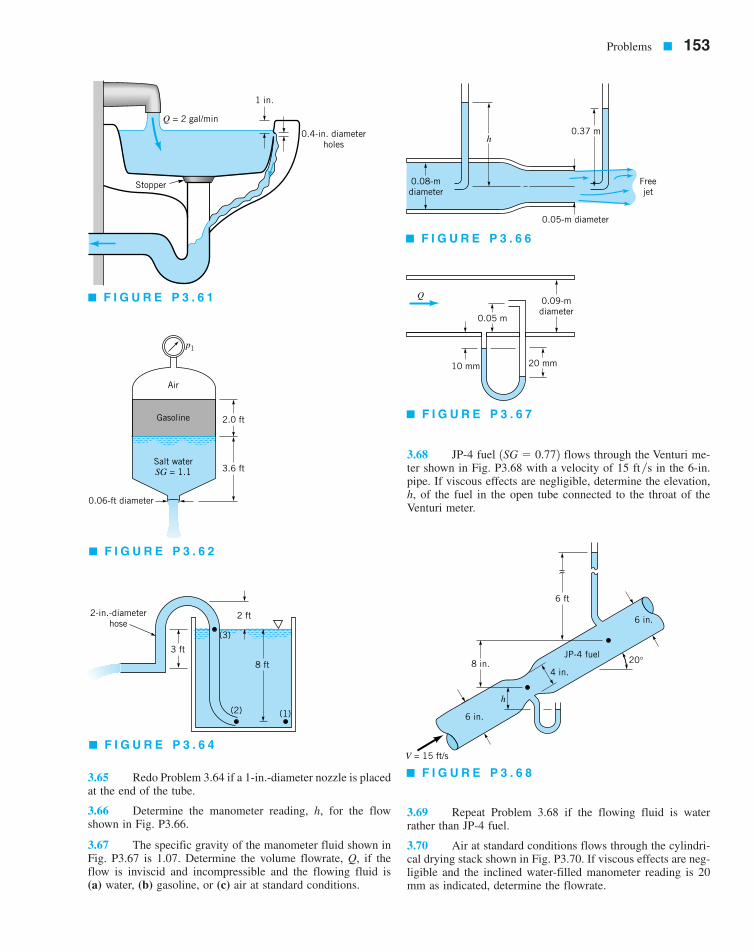
Problems � 153
3.65 Redo Problem 3.64 if a 1-in.-diameter nozzle is placedat the end of the tube.
3.66 Determine the manometer reading, h, for the flowshown in Fig. P3.66.
3.67 The specific gravity of the manometer fluid shown inFig. P3.67 is 1.07. Determine the volume flowrate, Q, if theflow is inviscid and incompressible and the flowing fluid is(a) water, (b) gasoline, or (c) air at standard conditions.
3.68 JP-4 fuel flows through the Venturi me-ter shown in Fig. P3.68 with a velocity of 15 ft�s in the 6-in.pipe. If viscous effects are negligible, determine the elevation,h, of the fuel in the open tube connected to the throat of theVenturi meter.
3.69 Repeat Problem 3.68 if the flowing fluid is waterrather than JP-4 fuel.
3.70 Air at standard conditions flows through the cylindri-cal drying stack shown in Fig. P3.70. If viscous effects are neg-ligible and the inclined water-filled manometer reading is 20mm as indicated, determine the flowrate.
1SG � 0.772
Q = 2 gal/min
1 in.
0.4-in. diameterholes
Stopper
� F I G U R E P 3 . 6 1
Air
p1
Gasoline
Salt waterSG = 1.1
0.06-ft diameter
3.6 ft
2.0 ft
� F I G U R E P 3 . 6 2
2-in.-diameterhose
3 ft
2 ft
8 ft
(2) (1)
(3)
� F I G U R E P 3 . 6 4
h0.37 m
0.05-m diameter
Freejet
0.08-mdiameter
� F I G U R E P 3 . 6 6
Q
0.05 m
10 mm 20 mm
0.09-mdiameter
� F I G U R E P 3 . 6 7
V = 15 ft/s
h
6 in.
8 in.4 in.
JP-4 fuel
6 ft
6 in.
20°
� F I G U R E P 3 . 6 8
7708d_c03_100-159 7/5/01 8:27 AM Page 153
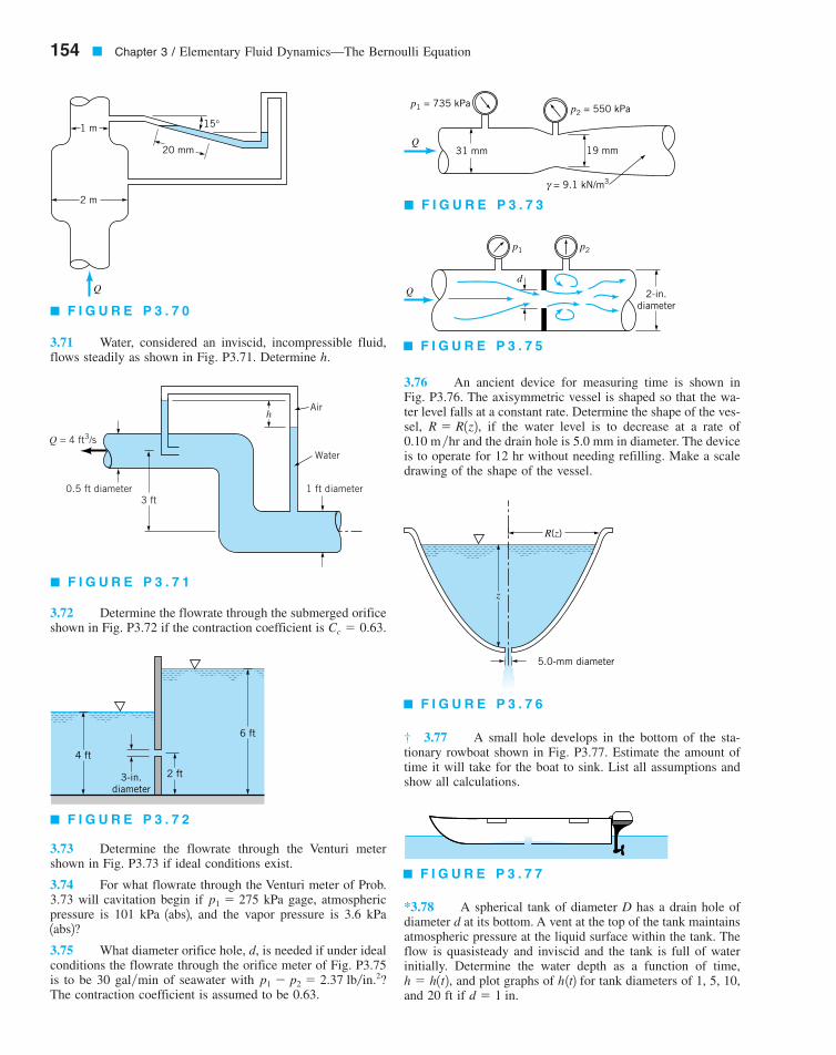
3.71 Water, considered an inviscid, incompressible fluid,flows steadily as shown in Fig. P3.71. Determine h.
3.72 Determine the flowrate through the submerged orificeshown in Fig. P3.72 if the contraction coefficient is
3.73 Determine the flowrate through the Venturi metershown in Fig. P3.73 if ideal conditions exist.
3.74 For what flowrate through the Venturi meter of Prob.3.73 will cavitation begin if kPa gage, atmosphericpressure is 101 kPa 1abs2, and the vapor pressure is 3.6 kPa1abs2?
3.75 What diameter orifice hole, d, is needed if under idealconditions the flowrate through the orifice meter of Fig. P3.75is to be 30 gal�min of seawater with The contraction coefficient is assumed to be 0.63.
3.76 An ancient device for measuring time is shown inFig. P3.76. The axisymmetric vessel is shaped so that the wa-ter level falls at a constant rate. Determine the shape of the ves-sel, if the water level is to decrease at a rate of0.10 m�hr and the drain hole is 5.0 mm in diameter. The deviceis to operate for 12 hr without needing refilling. Make a scaledrawing of the shape of the vessel.
3.77 A small hole develops in the bottom of the sta-tionary rowboat shown in Fig. P3.77. Estimate the amount oftime it will take for the boat to sink. List all assumptions andshow all calculations.
*3.78 A spherical tank of diameter D has a drain hole ofdiameter d at its bottom. A vent at the top of the tank maintainsatmospheric pressure at the liquid surface within the tank. Theflow is quasisteady and inviscid and the tank is full of waterinitially. Determine the water depth as a function of time,
and plot graphs of h 1t2 for tank diameters of 1, 5, 10,and 20 ft if d � 1 in.h � h1t2,
†
R � R1z2,
p1 � p2 � 2.37 lb�in.2?
p1 � 275
Cc � 0.63.
154 � Chapter 3 / Elementary Fluid Dynamics—The Bernoulli Equation
1 m
20 mm
15°
2 m
Q
� F I G U R E P 3 . 7 0
0.5 ft diameter 1 ft diameter
Q = 4 ft3/s
3 ft
Water
Airh
� F I G U R E P 3 . 7 1
2 ft
6 ft
4 ft
3-in.diameter
� F I G U R E P 3 . 7 2
z
5.0-mm diameter
R(z)
� F I G U R E P 3 . 7 6
p1 = 735 kPa p2 = 550 kPa
Q19 mm31 mm
γ = 9.1 kN/m3
� F I G U R E P 3 . 7 3
� F I G U R E P 3 . 7 7
p1 p2
2-in.diameter
dQ
� F I G U R E P 3 . 7 5
7708d_c03_154 8/13/01 6:43 PM Page 154
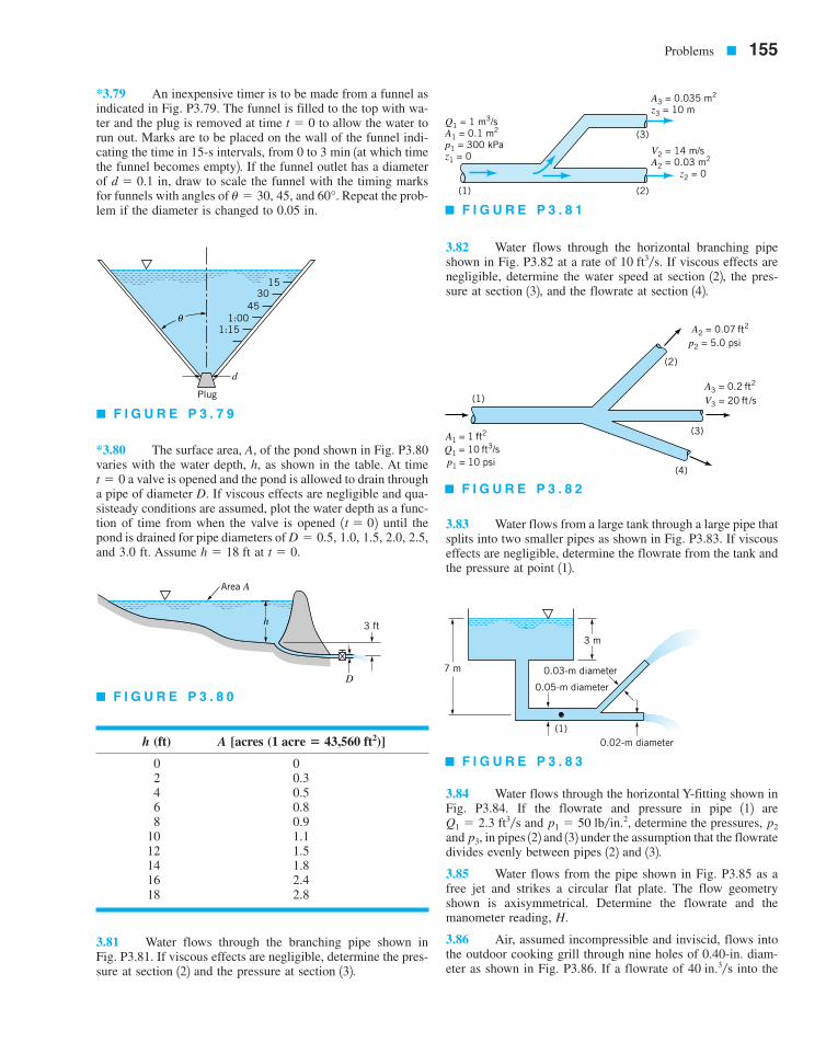
*3.79 An inexpensive timer is to be made from a funnel asindicated in Fig. P3.79. The funnel is filled to the top with wa-ter and the plug is removed at time to allow the water torun out. Marks are to be placed on the wall of the funnel indi-cating the time in 15-s intervals, from 0 to 3 min 1at which timethe funnel becomes empty2. If the funnel outlet has a diameterof in, draw to scale the funnel with the timing marksfor funnels with angles of and . Repeat the prob-lem if the diameter is changed to 0.05 in.
*3.80 The surface area, A, of the pond shown in Fig. P3.80varies with the water depth, h, as shown in the table. At time
a valve is opened and the pond is allowed to drain througha pipe of diameter D. If viscous effects are negligible and qua-sisteady conditions are assumed, plot the water depth as a func-tion of time from when the valve is opened until thepond is drained for pipe diameters of and 3.0 ft. Assume at .
3.81 Water flows through the branching pipe shown inFig. P3.81. If viscous effects are negligible, determine the pres-sure at section 122 and the pressure at section 132.
3.82 Water flows through the horizontal branching pipeshown in Fig. P3.82 at a rate of If viscous effects arenegligible, determine the water speed at section 122, the pres-sure at section 132, and the flowrate at section 142.
3.83 Water flows from a large tank through a large pipe thatsplits into two smaller pipes as shown in Fig. P3.83. If viscouseffects are negligible, determine the flowrate from the tank andthe pressure at point 112.
3.84 Water flows through the horizontal Y-fitting shown inFig. P3.84. If the flowrate and pressure in pipe 112 are
and determine the pressures,and in pipes 122 and 132 under the assumption that the flowratedivides evenly between pipes 122 and 132.3.85 Water flows from the pipe shown in Fig. P3.85 as afree jet and strikes a circular flat plate. The flow geometryshown is axisymmetrical. Determine the flowrate and themanometer reading, H.
3.86 Air, assumed incompressible and inviscid, flows intothe outdoor cooking grill through nine holes of 0.40-in. diam-eter as shown in Fig. P3.86. If a flowrate of into the40 in.3�s
p3,p2p1 � 50 lb�in.2,Q1 � 2.3 ft3�s
10 ft3�s.
t � 0h � 18 ftD � 0.5, 1.0, 1.5, 2.0, 2.5,
1t � 02
t � 0
60°u � 30, 45,d � 0.1
t � 0
Problems � 155
1530
451:00
1:15θ
Plug
d
� F I G U R E P 3 . 7 9
A1 = 1 ft2
Q1 = 10 ft3/sp1 = 10 psi
A2 = 0.07 ft2
p2 = 5.0 psi
(2)
A3 = 0.2 ft2
V3 = 20 ft /s
(4)
(3)
(1)
� F I G U R E P 3 . 8 2
7 m
3 m
0.05-m diameter
0.03-m diameter
0.02-m diameter(1)
� F I G U R E P 3 . 8 3
Area A
h
D
3 ft
� F I G U R E P 3 . 8 0
(1) (2)
(3)
V2 = 14 m/sA2 = 0.03 m2
z2 = 0
Q1 = 1 m3/sA1 = 0.1 m2
p1 = 300 kPa z1 = 0
A3 = 0.035 m2
z3 = 10 m
� F I G U R E P 3 . 8 1
h (ft) A [acres ( )]
0 02 0.34 0.56 0.88 0.9
10 1.112 1.514 1.816 2.418 2.8
1 acre � 43,560 ft2
7708d_c03_100-159 7/5/01 8:27 AM Page 155
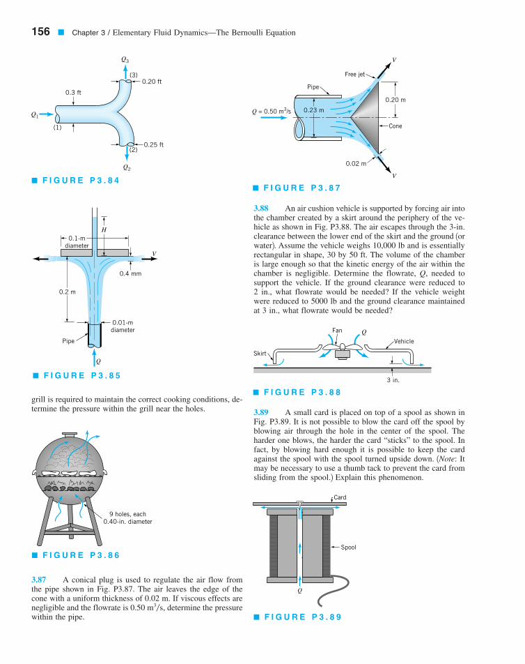
grill is required to maintain the correct cooking conditions, de-termine the pressure within the grill near the holes.
3.87 A conical plug is used to regulate the air flow fromthe pipe shown in Fig. P3.87. The air leaves the edge of thecone with a uniform thickness of 0.02 m. If viscous effects arenegligible and the flowrate is determine the pressurewithin the pipe.
3.88 An air cushion vehicle is supported by forcing air intothe chamber created by a skirt around the periphery of the ve-hicle as shown in Fig. P3.88. The air escapes through the 3-in.clearance between the lower end of the skirt and the ground 1orwater2. Assume the vehicle weighs 10,000 lb and is essentiallyrectangular in shape, 30 by 50 ft. The volume of the chamberis large enough so that the kinetic energy of the air within thechamber is negligible. Determine the flowrate, Q, needed tosupport the vehicle. If the ground clearance were reduced to2 in., what flowrate would be needed? If the vehicle weightwere reduced to 5000 lb and the ground clearance maintainedat 3 in., what flowrate would be needed?
3.89 A small card is placed on top of a spool as shown inFig. P3.89. It is not possible to blow the card off the spool byblowing air through the hole in the center of the spool. Theharder one blows, the harder the card “sticks” to the spool. Infact, by blowing hard enough it is possible to keep the cardagainst the spool with the spool turned upside down. 1Note: Itmay be necessary to use a thumb tack to prevent the card fromsliding from the spool.2 Explain this phenomenon.
0.50 m3�s,
156 � Chapter 3 / Elementary Fluid Dynamics—The Bernoulli Equation
(1)
(2)
(3)0.20 ft
0.25 ft
0.3 ft
Q1
Q2
Q3
� F I G U R E P 3 . 8 4
Vehicle
Fan
Skirt
3 in.
Q
� F I G U R E P 3 . 8 8
V
0.2 m
0.01-mdiameter
0.4 mm
0.1-mdiameter
H
Q
Pipe
� F I G U R E P 3 . 8 5
9 holes, each0.40-in. diameter
� F I G U R E P 3 . 8 6
Q
Card
Spool
� F I G U R E P 3 . 8 9
0.23 mQ = 0.50 m3/s
Pipe
Free jet
0.20 m
V
V
0.02 m
Cone
� F I G U R E P 3 . 8 7
7708d_c03_100-159 7/5/01 8:27 AM Page 156
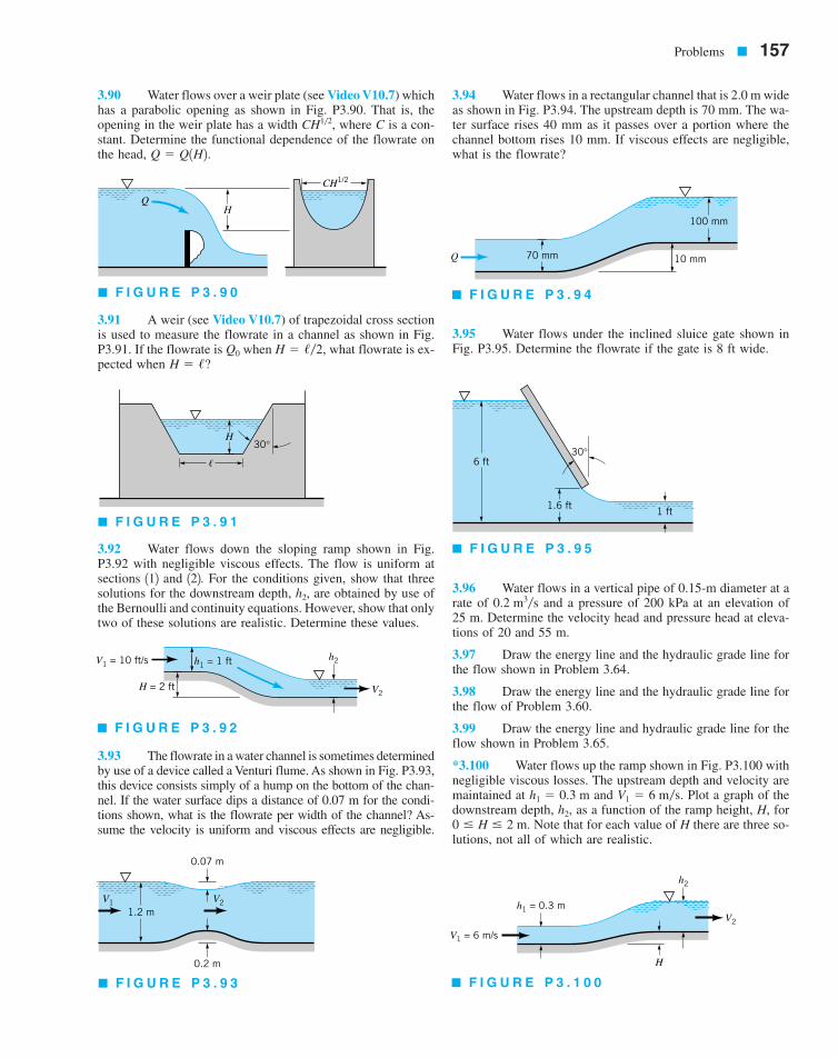
3.90 Water flows over a weir plate (see Video V10.7) whichhas a parabolic opening as shown in Fig. P3.90. That is, theopening in the weir plate has a width where C is a con-stant. Determine the functional dependence of the flowrate onthe head,
3.91 A weir (see Video V10.7) of trapezoidal cross sectionis used to measure the flowrate in a channel as shown in Fig.P3.91. If the flowrate is when what flowrate is ex-pected when
3.92 Water flows down the sloping ramp shown in Fig.P3.92 with negligible viscous effects. The flow is uniform atsections 112 and 122. For the conditions given, show that threesolutions for the downstream depth, are obtained by use ofthe Bernoulli and continuity equations. However, show that onlytwo of these solutions are realistic. Determine these values.
3.93 The flowrate in a water channel is sometimes determinedby use of a device called a Venturi flume. As shown in Fig. P3.93,this device consists simply of a hump on the bottom of the chan-nel. If the water surface dips a distance of 0.07 m for the condi-tions shown, what is the flowrate per width of the channel? As-sume the velocity is uniform and viscous effects are negligible.
3.94 Water flows in a rectangular channel that is 2.0 m wideas shown in Fig. P3.94. The upstream depth is 70 mm. The wa-ter surface rises 40 mm as it passes over a portion where thechannel bottom rises 10 mm. If viscous effects are negligible,what is the flowrate?
3.95 Water flows under the inclined sluice gate shown inFig. P3.95. Determine the flowrate if the gate is 8 ft wide.
3.96 Water flows in a vertical pipe of 0.15-m diameter at arate of and a pressure of 200 kPa at an elevation of25 m. Determine the velocity head and pressure head at eleva-tions of 20 and 55 m.
3.97 Draw the energy line and the hydraulic grade line forthe flow shown in Problem 3.64.
3.98 Draw the energy line and the hydraulic grade line forthe flow of Problem 3.60.
3.99 Draw the energy line and hydraulic grade line for theflow shown in Problem 3.65.
*3.100 Water flows up the ramp shown in Fig. P3.100 withnegligible viscous losses. The upstream depth and velocity aremaintained at and Plot a graph of thedownstream depth, as a function of the ramp height, H, for
Note that for each value of H there are three so-lutions, not all of which are realistic.0 � H � 2 m.
h2,V1 � 6 m �s.h1 � 0.3 m
0.2 m3�sh2,
H � /?H � /�2,Q0
Q � Q1H2.CH1�2,
Problems � 157
Q
CH1/2
H
� F I G U R E P 3 . 9 0
H
�
30°
� F I G U R E P 3 . 9 1
V1 = 10 ft/s h1 = 1 ft h2
H = 2 ft V2
� F I G U R E P 3 . 9 2
1.2 m
0.2 m
0.07 m
V1 V2
� F I G U R E P 3 . 9 3
Q 10 mm
100 mm
70 mm
� F I G U R E P 3 . 9 4
6 ft
1.6 ft1 ft
30°
� F I G U R E P 3 . 9 5
V1 = 6 m/s
V2
H
h2
h1 = 0.3 m
� F I G U R E P 3 . 1 0 0
7708d_c03_100-159 7/5/01 8:27 AM Page 157
3.101 This problem involves the pressure distribution be-tween two parallel circular plates. To proceed with this prob-lem, click here in the E-book.
3.102 This problem involves the calibration of a nozzle-type flow meter. To proceed with this problem, click here inthe E-book.
3.103 This problem involves the pressure distribution in atwo-dimensional channel. To proceed with this problem, clickhere in the E-book.
3.104 This problem involves the determination of theflowrate under a sluice gate as a function of the water depth.To proceed with this problem, click here in the E-book.
158 � Chapter 3 / Elementary Fluid Dynamics—The Bernoulli Equation
7708d_c03_100-159 7/6/01 10:45 AM Page 158