fluid–structure interaction analysis of sloshing in an

Ocean Systems Engineering, Vol. 3, No. 3 (2013) 181-201 DOI: http://dx.doi.org/10.12989/ose.2013.3.3.181 181

Copyright © 2013 Techno-Press, Ltd. http://www.techno-press.org/?journal=ose&subpage=7 ISSN: 2093-6702 (Print), 2093-677X (Online)

Fluid–structure interaction analysis of sloshing in an annular - sectored water pool subject to surge motion

M. Eswaran, P. Goyal, G.R. Reddy, R.K. Singh and K.K. Vaze

Bhabha Atomic Research Centre, Mumbai, 400085, India

(Received January 11, 2013, Revised July 12, 2013, Accepted July 31, 2013)

Abstract. The main objective of this work is to investigate the sloshing behavior in a baffled and unbaffled three dimensional annular-sectored water pool (i.e., tank) which is located at dome region of the primary containment. Initially two case studies were performed for validation. In these case studies, the theoretical and experimental results were compared with numerical results and good agreement was found. After the validation of present numerical procedure, an annular-sectored water pool has been taken for numerical investigation. One sector is taken for analysis from the eight sectored water pool. The free surface is captured by Volume of Fluid (VOF) technique and the fluid portion is solved by finite volume method while the structure portions are solved by finite element approach. Baffled and un-baffled cases were compared to show the reduction in wave height under excitation. The complex mechanical interaction between the fluid and pool wall deformation is simulated using a partitioned strong fluid–structure coupling.

Keywords: liquid sloshing; free surface; numerical simulation; annular-sectored water pool; fluid-structure interaction 1. Introduction

For the last few decades, liquid sloshing is an important problem in several areas including nuclear, aerospace, and seismic engineering. Considering the safety aspects of the liquid containing structures, liquid sloshing is one of the significant problems in many engineering divisions. Particularly, considering the load on the structure due to liquid sloshing is thus very important for the Nuclear Power Plants (NPPs) structure to ensure structural integrity, its withstand capacity against dynamic pressure loads due to liquid oscillations. Such an oscillatory motion of the liquid in its container is called as sloshing. Under the seismic load, severe accidents might be possible due to this kind of oscillatory motions. This dynamic load can cause possible leakage (Malhotra, 1997), pollution to the surrounding area, and elephant-foot buckling due to bending of the tank (Ibrahim, 2005) wall in the containment structure.

To extract and utilize the nuclear power safely and continuously, technology development for enhanced safety is vital for future nuclear power plants. As discussed by Lee at al. (2013), at the beginning of the 1950s, the USA and USSR began to develop floating nuclear power plants (FNPPs). Now days, various nuclear societies are focusing their studies towards floating, GBS

Corresponding author, Scientific Officer, E-mail: [email protected]


type, and submerged offshore nuclear power plants (ONPP) (Gerwick 2007, Lee et al. 2011). To

enhance the safety of nuclear power, the conventional nuclear power plant (NPP) can be moved

from land to ocean. However, most of the present working nuclear reactors are land-based. And

some of the future land-based reactors are also being designed with improved safety features by

various societies.

The typical Indian advanced reactors are land-based with enhanced safety features which have

an annular-sectored water pool on its dome region of the primary containment in reactor building

(Sinha and Kakodkar 2006). This present work is focusing the liquid sloshing in such a large pool

of advanced reactor. The water in the pool serves as a heat sink for the residual heat removal

system and several other passive systems. As reported by Sinha and Kakodkar (2006), this annular

water pool is divided into eight compartments as shown in Fig. 1, which are interconnected to each

other. Each compartment of water pool contains an isolation condenser for core decay heat

removal during shutdown. Water in the pool is used to condense the steam flowing through the

isolation condenser during reactor shutdown and also function as a suppression pool to cool the

steam and air mixture during Loss of Coolant Accident (LOCA). This water pool provides cooling

to the fuel in passive mode during first fifteen minutes of LOCA by high pressure injection from

advanced accumulators and later for three days.

2.1 Problem definition and objectives

To ensure the safety of the reactor against the seismic load, the annular-sectored water pool

located on the primary containment should be investigated. The present work is mainly focused on

liquid sloshing inside the water pool under harmonic excitation. The liquid height has been

estimated in first mode natural frequency for different amplitudes, water spilled out conditions,

different type of baffle and its effect on liquid oscillations have taken as key findings of this

present investigation. In addition to this, the pressure and wall displacement are also estimated.

The simple rectangular and cylindrical tanks have a detailed analytical solution procedure to

find the natural frequency, pressure load and liquid elevations. However, the analytical procedure

(a) Isometric view (b) Plan

Fig. 1 Eight-sectored water pool located top of the primary containment

182

Fluid - structure interaction analysis of sloshing in an annular - sectored water pool…

for the baffled annularsectored water pools with considerable interaction effects is very difficult to

determine. Many numerical and experimental works has been reported on sloshing for regular

geometries with different aspects, although only few studies have assessed the baffled asymmetric

geometries. This work is focused on liquid sloshing in an annular-sectored water pool with and

without baffles. For prediction of slosh height in such complicated geometries, a Computational

Fluid Dynamics (CFD) software can be very useful as a simulation tool. The commercial CFD

software ESI, CFD-ACE+, Version 2011 (ESI-CFD, Inc., Huntsville, AL) is employed for

numerical calculations to explore the interaction of the water pool wall and liquid during liquid

sloshing. The program consists of three main parts, CFD-GEOM for geometry and grid generation,

CFD-GUI for setting boundary and initial conditions and CFD-VIEW as an interactive

visualization program.

The objectives of this present work are to investigate (i) First mode sloshing frequency of the

liquid. (ii) Slosh heights and conditions for water spilled (i.e., under what conditions, the water

will be spilled out during sloshing). (iii) Effect of annular and cap-plate baffles to prevent

excessive sloshing. (iv) The water pool wall displacement and stress induced due to the liquid load.

(v) Effect of higher modes on liquid sloshing. In section 2, theoretical formulation has been

established for fluid and structural domains to explore the fluid–structure interaction phenomena

for a moving liquid water pool. Section 3 explains the numerical approach and the frequency

modes of liquid and structural domains. The result and discussions were given in section 4, which

is divided into five sub-sections. First two sub-sections are focused on the experimental and

analytical validation with the present numerical approach. The remaining sub-sections are focused

on the numerical investigation on annular-sectored water pool with and without baffles. Here, the

slosh arresting power of annular and cap-plate baffle is discussed while considering the fluid-

structure interaction.

2. Theoretical formulations for FSI

The model on the fluid domain is based on the three-dimensional time-dependent conservation

equations of mass and momentum to determine the sloshing characteristics. For the structure

domain, the equation of motion is utilized to simulate the displacement of the concrete wall.

2.1 Fluid formulation The forces acting on the fluid in order to conserve momentum must balance the rate of change

of momentum of fluid per unit volume. For the laminar transient, incompressible flow with

constant fluid properties over the computational domain, the mass continuity and Navier–Stokes

equations are given as follows.

0 u

(1)

FuPuut

u

2 (2)

where F

is the external force vector and , are the dynamic viscosity and density of the

fluid respectively. The external force is the sum of the gravitational and applied forces. The u

183


and P denote the velocity vector and pressure of the oscillating fluid.

The aforementioned governing equations are discretized by the finite control volume approach

to replace the partial differential equations with the resulting algebraic equations for the entire

calculation region. Using the staggered-grid arrangement, grids of velocities are segregated from

grids of scalars and laid directly on the surfaces of the control volumes for estimating those

convective fluxes across cell surfaces. The well known Semi-Implicit Method for Pressure-Linked

Equations Consistent (SIMPLEC) numerical algorithm is employed for the velocity–pressure

coupling. In SIMPLEC, an equation for pressure-correction is derived from the continuity equation

which governs mass conservation. It is an inherently iterative method. The under-relaxation

technique is also implemented to circumvent divergence during iterations. The velocities and local

pressure can be determined until convergent criteria are satisfied.

2.2 Structural formulation

In the structure model, the linear elasticity approach is utilized with the solid portions. After the

finite element analysis of the solid wall under the slosh loading condition, the following solid wall

displacement caused by the fluid–structure interactions is assumed to be small and linear. Hence to

simulate the motion of solid portions, the governing equations are written as below.

xszxyxxx

s gzyxt

s

2

2

(3)

ys

zyxyyy

s gzxyt

s

2

2

(4)

zs

yzxzzzs g

yxzt

s

2

2

(5)

Here, s and xs are the structure density and structure displacement respectively. The linear

stress– strain relation can be expressed as 0 oD

. Here, 0 and 0 are initial strains

and stresses respectively. Here, the symbol D is the elasticity matrix containing the material

properties. A finite element method is used to solve the solid model with the principal of virtual

work. For each element, displacements are defined at the nodes and obtained within the element by

interpolation from the nodal values using shape functions. Structural domains are meshed using

similar first order quadrilateral elements. Eqs. (3) through (5) can be linear or nonlinear, depending

on the constitutive relations used for the material in consideration and whether the displacements

are small or large (Bathe 1966).

2.3 Coupling between fluid flows and structural media

The coupling of the fluid and structural response can be attained numerically in different ways,

however in all cases, of course, the conditions of displacement compatibility and traction

equilibrium along the structure–fluid interfaces ( si ) must satisfy the following conditions.

(i) The fluid and solid wall move concurrently (displacement compatibility).

184


ssf iondd (6)

(ii) The fluid force (pressure and shear stress) applying on the solid wall is identical to the wall

force exerted to the liquid side (Traction equilibrium).

ssf ionff (7)

where, fd and sd are the displacements, ff and sf are the tractions of the fluid and solid,

respectively, and si is the interface of the fluid and solid domains. These conditions must be

imposed efficiently in the numerical solution. In this problem, the solutions are based on

partitioned method where separate solutions for the different domains are prepared. One solution is

for fluid and other is for structure from the independent solvers. At the fluid-structure interface,

information for the solution is shared between the fluid solver and structure solver. The

information is exchanged at interface based on the coupling method. Two way coupling is adopted

for calculations (Benra et al. 2011).

3. Numerical investigation

Here, an annular eight-sectored water pool as depicted in Figs. 1(a) and 1(b), is taken for

analysis. One sector is taken from suppression pool for analysis. Here three domains are modeled

viz., water pool wall, liquid and air domains. The sketch and dimensions of the water pool are

depicted in Fig. 2. The side wall thickness is 500 mm and bottom is 1000mm. Height of the water

and air is 8 m and 1 m respectively.

Tank wall

Air

Water

16000

R 27800

R 7000

10000

Fig. 2 One compartment of annular water pool

185


3.1 Grid generation and boundary conditions

A grid is an artificial geometric construction that assists spatial discretization of the governing

equations to be solved. Here, block structured grid (BSG) has been used to generate the grid, i.e.,

the flow domain is split up into a number of topographically simpler domains and each domain is

meshed separately and joined up correctly with neighbours. The BSG arrangement for un-baffled

and baffled water pool has been shown respectively in Figs. 3 and 4. The fluid-structure

interaction is considered by appropriately coupling the nodes that lie in the common element faces

of the two (i.e., fluid and structure) domains. Fig. 4 clearly shows that the fluid and structure

domains share the common element face at fluid-structure interface which may lead to better data

transformation between domains. The fluid domain is divided into 18,000 sub domains and

structure wall into 8000. The values of warpage and jacobian matrix are found within acceptable

limits.

Fig. 3 Numerical grid of un-baffled annular-sectored

water pool

Fig. 4 Block structured mesh on fluid and structure

portions

The NS equation is solved in each sub volumes in the fluid domains (liquid and air). Cell

centered average value is taken into consideration. In calculations, the material properties used for

Fluid-structure Interaction (FSI) simulations are summarized in Table 1. Top boundary of the air is

fixed pressure condition (at atmosphere condition). Implicit pressure and implicit shear wall

condition is applied on the fluid-structure interfaces. The calculations require 400 iterations to

satisfy convergence with absolute velocity residual 10-6< R< 10-8.

The choice of method used for the solution of the assembled system of equations can have a

major impact on the overall solution time and solution quality. Here, the algebraic multigrid is

used for solving the system of linear equations. The basic idea of a multigrid solution is to use a

hierarchy of grids, from fine to coarse, with each grid being particularly effective for smoothing

the errors at the characteristic wavelength of the mesh spacing on that grid. Other iterative solvers

are non-optimal in the sense that as the mesh resolution increases, the convergence rate degrades.

(ESI CFD Inc 2011). The simulation was carried out on an Intel Xeon, 2.8 GHz six core processor

186


workstation and the simulation ran for approximately 32 CPU hours for each case (solution up to

20 seconds). The implicit scheme is used for temporal integration and the higher order upwind

schemes are used for the spatial discretization. The free surface elevation ( ) has been captured

every 0.05 second.

For modeling free surface flows, marker and cell (Chen et al. 1997), VOF, level set method,

sigma-transformation (Frandsen 2004, Chen and Nokes 2005, Eswaran and Saha 2009, 2010,

2011) and meshless method based on smoothed particle hydrodynamics (Vorobyev et al. 2011) are

known methods. Neverthless, this work adopts VOF method. The VOF method is developed by

Hirt and Nichols (1981) and refined thereafter by various authors. Since the method is designed for

two or more immiscible fluids, a portion of air is filled above the liquid level for all cases. The air

portion is also modeled and discretized using the 3-D fluid element. In this method, the term, first

fluid and second fluid indicate the air and water domains respectively. It is based on tracking a

scalar field variable F which stands for the distribution of the second fluid in the computational

grid. F specifies the fraction of the volume of each computational cell in the grid occupied by the

second fluid. All cells containing only fluid 2 will take the value F = 1 and cells completely filled

with fluid 1 is represented by F = 0. Cells containing an interface between air and water take on a

value of F between 0 and 1. For a given flow field with the velocity vector u and an initial

distribution of F on a grid, the volume fraction distribution F (and hence the distribution of fluid

two) is determined by the passive transport equation

0

Fu

t

F (8)

This equation must be solved jointly with the primary equations of conservation of mass and

momentum, to achieve computational coupling between the velocity field solution and the liquid

distribution. From the F distribution the interface between the two fluid phases has to be

reconstructed at every time step. As depicted in the manual (ESI CFD Inc 2011, Glatzel et al.

2008), the VOF method in CFD-ACE+ offers some additional features like an algorithm to remove

the so called flotsam and jetsam caused due to numerical errors. It is characterized by the

generation of tiny isolated droplets of liquids or gas in the regions of the other medium, especially

in regions of high swirl.

4. Results and discussion

The total fluid dynamic pressure for a flexible tank partially filled with liquid undergoing a

seismic motion consists of three components. The first pressure component is called the impulsive

pressure which varies synchronously with the tank base input motion. The tank wall is assumed to

be rigid, moving together with the tank base. The second component is caused by the fluid

sloshing motion. This pressure is generally referred to as the convective pressure or non impulsive

pressure, while the third component is induced by the relative motion of the flexible tank wall with

respect to the tank base (Chang et al. 1989). This fluid-structure interaction effect results in the

dynamic characteristics of the tank-liquid system to be notably different from that of a fixed tank

has led to the inclusion of a third hydrodynamic component to quantify the dynamic response of

flexible tanks namely the „flexible-impulsive‟ component. Methods for determining the

contribution of the flexible-impulsive component to the total response (base shear, overturning

187


moments, wall stresses) of tanks under seismic excitations have been proposed by various

researchers (Haroun and Housner 1981, Tedesco et al. 1989).

In this study, the problems are restricted to the tank under surge motion. During analysis, the

complete flow regime is assumed to be laminar. Some localized turbulence effects may be caused

at the sheared interface during sloshing which should not affect the fluid-wall interactions and

global fluid behavior. This type of gravity force dominant flow problems are mainly considered as

inviscid. It had been exposed that the free surface oscillations of low viscosity fluids in partly-

filled tank persist over long durations (Kandasamy et al. 2010). To validate the present numerical

procedure, the two case studies have been carried out. In the first case study, a 2-D tank with fixed

wall assumption has taken and the elevation is compared with analytical and present numerical

procedure to ensure the accuracy of the solver while, the second case study is performed to

compare with experimental results for sectored and non-sectored tank.

4.1 Case study 1: analytical validation

In this section, a 2D model partially filled tank has been taken and the liquid elevation has been

captured under sinusoidal excitation by numerical as well as analytical relation. The 2-D rigid tank

which is 570 mm long and 300 mm high is excited with )sin( tA as shown in Fig. 5. The water

depth is 150 mm and excited amplitude is 5 mm. The lowest natural frequency 1 for this case is

6.0578 rad/sec. The natural frequency is calculated from Eq. (10). Liquid free surface elevation

has been calculated from the following third order analytical relations (Faltinsen et al. 2000) and

compared with the present numerical simulation results for frequency ratio 0.583.

)2cos(

)cos()4(

3

2

1)2cos(*

)4(2

33

8

1

8

1

)cos()cos(),(

22

2

22

2242

2

2

2

2

22

224

4

224

4

224

2

xk

tkg

t

kgkgkg

g

axktatx n

n

nnn

nnnnn

nnn

nn

n

nn

n

nn

nnn

(9)

where the linear sloshing frequencies

)tanh( snnn hkgk and )2tanh(22 snnn hkkg (10)

The initial conditions are )cos(),(0

xkanx xt

and 0),(

0

tzx , where a is the amplitude

of the initial wave profile, bnkn / is the wave profile for n = 0,1,2... and x is the horizontal

distance from the left wall. This analytical result is compared with the present numerical approach.

From Fig. 6, it is observed that the free surface elevation of analytical and present numerical

coincides with each other. In this analytical method, the free surface is calculated exactly at 20 cm

from the left side of the tank. However, the numerical is not possible exactly at 20 cm from the left.

So the grid point location very close to 20 cm from the left wall is taken which is around 19.6 cm.

This causes a very small discrepancy near trough and crest of the wave in Fig. 6.

4.2 Case study 2: experimental validation

This case study shows the comparison of experimental and numerical results. For this purpose,

a model square tank with sectored arrangement was built and experiments were conducted at

BARC, Mumbai. The experiments were performed on a shake table (1.2 m x 1.0 m) coupled with

188


a servo-controlled hydraulic actuator of 250 KN capacity. The test setup is specially designed for

the sloshing experiments as shown in Fig. 7. The perspective view of the setup is shown in Fig. 8

with the actuator coupling arrangement.

570

Probe

20

All dimensions are in mm

Water

Air

300x

y

Time (Sec)F

ree

su

rfa

ce

ele

va

tio

n(m

)0 2 4 6 8 10

-0.015

-0.01

-0.005

0

0.005

0.01

0.015

Analytical

Present Numerical

Fig. 5 The sketch of the 2-D rigid rectangular tank Fig. 6 Comparisons of free surface elevation

Platform

LiquidA sin (ω t)

DAS

10

020

0

50

025

0

1000

Fig. 7 Details of the experimental setup

A square tank of 1 meter length and 0.5 meter height along with removable 4-sector

arrangement is built as shown in Fig. 9 for the experiments in order to allow liquid motions in all

directions. Pressure variations are sensed by two flush type pressure transducers installed at 100

mm (position 1) and 200 mm (position 2) from the bottom of the tank. Water fill level in the tank

is maintained as 250 mm. For this case the liquid natural frequency has been calculated as 0.71 Hz

through analytical relation and sine sweep experiments. The comparison of experimental and

numerical time history of pressure at position 2 for simple square tank and 4- sectored square tank

cases are shown in Figs. 10(a) and 10(b) respectively. For these cases, the excitation frequency

ratio is taken as 0.57 and 0.99 of the first mode simple square tank. The comparisons of numerical

with experiment results are shown that numerical data has close match with the experiment.

189


Fig. 8 Experimental setup Fig. 9 Isometric view of 4-sectored square tank

mode

0 1 2 3 4 5 6 7 8 9 10

0

100

200

300

400

500

600

700

800

Numerical

Experimental

Pre

ss

ure

(P

a)

Time (Sec)

0 1 2 3 4 5 6 7 8 9 10

0

100

200

300

400

500

600

700

800

Pre

ss

ure

(P

a)

Time (Sec)

Numerical

Experimental

(a) Simple square tank at excitation frequency 0.57

1 .

(b) Sectored square tank at excitation frequency

0.99 1 .

Fig. 10 Comparison of experimental and numerical pressure data at 200 mm from tank bottom (position 2)

4.3 Numerical investigation on annular-sectored water pool

The above two case studies were performed for the validation of the numerical procedure

followed and checked the solver performance for sectored and non-sectored arrangement of the

water pool.

4.3.1 Model analysis of the annular-sectored water pool The sinusoidal excitation is applied on the fluid domain in terms of acceleration gravity force

via user subroutine functions. As discussed earlier, this annular water pool is dived in to eight

compartments. Among the eight, one compartment has taken for analysis. The sketch and

dimensions of the water pool are depicted in Fig. 2. The modal analysis is required to find the

inherent dynamic properties of the any domain in terms of its natural frequencies. In the beginning,

190


the first mode natural frequency of water pool has been calculated by free vibration i.e., free

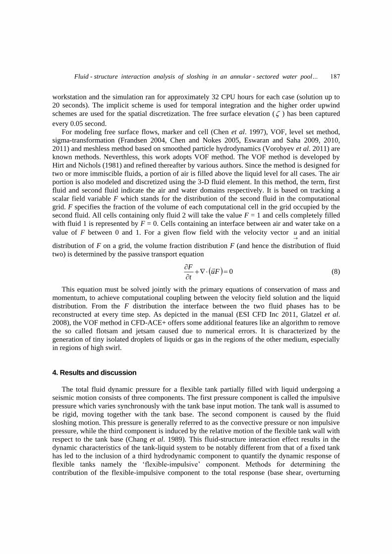
surface elevation ( ) of liquid under free vibration has been captured as represented in Fig. 11.

The first mode natural frequency is observed as 0.312 Hz by spectrum analysis from Fast

Fourier Transformation (FFT) (Fig. 12). The FFT is a faster version of the Discrete Fourier

Transform (DFT). The FFT utilizes some clever algorithms in much less time than DFT. The FFT

is extremely important in the area of frequency (spectrum) analysis since it takes a discrete signal

in the time domain and converts that signal into its discrete frequency domain representation. The

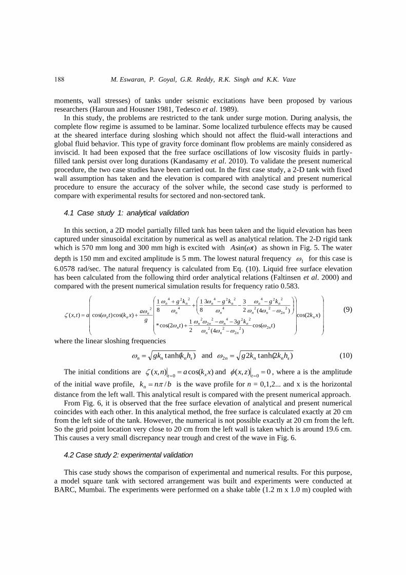
dominant modes of the structure i.e., the first four mode shapes are illustrated in Fig. 13. The case

studies for numerical simulation were summarized in Table 2.

0 2 4 6 8 10 12 14-1500

-1000

-500

0

500

1000

1500

Fre

e s

urf

ac

e e

lev

ati

on

(m

m)

Time (Sec)

0.0 0.2 0.4 0.6 0.8 1.0 1.2 1.4 1.6 1.8 2.0

0

50

100

150

200

1=0.312 Hz

Frequency (Hz)

Po

wer

Fig. 11 Free surface elevation of liquid under

free vibration Fig. 12 Spectrum analysis of signal

Table 1 Material properties

1 Water Kinematic

Viscosity 1 E-6 m2/sec Density 1000 kg/m3

2 Air Dynamic

Viscosity 1.846E-05 Kg/m sec Density 1.1614 kg/m3

3 Concrete

wall

Poisson's ratio 0.2 Density 2500 kg/m3

Young Modulus 33E+09 N/m2

Mode 1 (11.21 Hz) Mode 2 (17.61 Hz) Mode 3 (21.16 Hz) Mode 4 (27.89 Hz)

Fig. 13 Dominant mode shapes of structure

191


Table 2 Numerical experiments were conducted

Sl. No Baffle

Excitation

Amplitude

(m)

Excitation

Frequency

(Hz)*

Condition

1

No baffle

0.01 1

Fixed wall 2 0.02 1

3 0.06 1

4 0.1 1

5 0.1 1 Flexible wall

6

Annular 0.1

1

Flexible wall 7 5 1

8 10 1

9

Cap-Plate 0.1

1

Flexible wall 10 5 1

11 10 1

*First mode natural frequency of liquid is 1 =0.312 Hz

0 2 4 6 8 10 12 14 16 18 20 22 24-2

-1

0

1

2

Right

Left

Center

Time (Sec)

-2

-1

0

1

2

Right

Left

Center

Fre

e s

urf

ac

e E

lev

ati

on

(m

)

-2

-1

0

1

2

Right

-2

-1

0

1

2

x/

1 = 0.5

x/

1 = 0.8

x/

1 = 0.99

x/

1 = 1.2

(d)

(c)

(b)

(a)

Right

Left

Center

Fig. 14 Time history of free surface elevation at 0.1 m excitation amplitude and for different excitation

frequencies

192


4.3.2 Effect of excitation frequency of annular-sectored water pool Fig. 14 shows the numerical results for the liquid heights at the left, right and center point in a

three-dimensional annular-sectored water pool subject to harmonic motions under 0.1 m amplitude

for different frequencies.

When the excitation frequencies are close to the natural frequency as shown in Figs. 14(a) and

14(c), the beat phenomena are noticeable (Eswaran et al. 2009). It can be observed from Fig. 14

(d) that when the excitation frequency is far-off from the natural frequency, i.e., 1.92 rad /sec, the

liquid heights are very small and frequency is equal to excitation frequency. When the frequency is

almost near to the first mode natural frequency, i.e., Fig. 14(b), the amplitude grows monotonically

with time. There is a slight difference in liquid elevation between right and left corner of the water

pool.

0 2 4 6 8 10 12 14 16 18 20

-40

-20

0

20

40

Amplitute = 0.01 m

Time (Sec)

-40

-20

0

20

40

Amplitute = 0.02 m

/

A -40

-20

0

20

40

(d)

(c)

(b)

(a)

Amplitute = 0.06 m

-40

-20

0

20

40

Amplitute = 0.1 m (FSI)

Amplitute = 0.1 m (without FSI)

0.0 0.2 0.4 0.6 0.8 1.0 1.2 1.4 1.6 1.8 2.0

0.000

0.005

0.010

0.015

0.020

0.025

Frequency (Hz)

Po

wer

(a)

/A

(/

t)/(

A*

)

-15 -10 -5 0 5 10 15 20-1500

-1000

-500

0

500

1000

1500

(b)

Fig. 15 Time history of non-dimensional free surface

elevation at 1 =0.312 Hz for different

excitation amplitudes

Fig. 16 (a) Power spectral density for

amplitude 0.1 m and 1 =0.312 Hz

and (b) Phase-plane diagram for

amplitude 0.1 m and 1 =0.312 Hz

4.3.3 Effect of amplitude of annular-sectored water pool Figs. 15(a) through 15(d) depict the effect of excitation amplitude (A) under its first mode

193


natural frequency. For this purpose, the non-dimensional free surface elevation is captured at the

right corner of the water pool for 20 seconds. If the excitation amplitude is increased, the fluid

response becomes large around the first natural frequency. Fig. 15(a) is plotted with the

assumption of with and without fluid-structure interaction conditions. In the case of without FSI,

the boundaries are considered as rigid wall. It is also found in the Fig. 15(a) that FSI consideration

has slight more elevation than the without FSI. It is caused due to the interaction of the fluid

domain with structure produces the relative pressure component. However, there is a large gap

between the first mode frequency of the structure and fluid portions. Deviations are not high as the

excitation frequency is low and faraway from the structural first mode frequency. It is also

observed that the amplification of the fluid motion is relatively larger at lower amplitude while at

the higher amplitude; the amplification of free surface elevation is less than the lower amplitude

case. Fig. 16(a) shows the power spectral density of liquid elevation wave at 0.1 m excitation

amplitude. Closer to natural frequency, a single dominant frequency is absorbed. The phase-plane

diagram is plotted in Fig. 16(b) which shows that non-linearity exists in the flow.

Pressure waves are captured in different locations of the water pool and the locations (i.e., A

through E) are depicted in Fig. 17(a). Positions A through C are 1 m below from the liquid free

surface and positions D and E are in 5 m and 8 m from the free surface respectively. The time

histories of pressure at the different places of the water pool for un-baffled water pool are plotted

in Fig. 17(b) for 0.1 m amplitude sec and 1 w =0.312 Hz. It can be seen from the Fig. that when

the water pool is excited, the impulse pressures occur because of the relatively large amplitude of

the external excitation. If liquid oscillation is not controlled efficiently, sloshing of liquids in

storage water pools may lead to large dynamic stress to cause structural failure. On the other hand,

if the baffle exists in the water pool, the impulse pressures will be removed. The horizontal

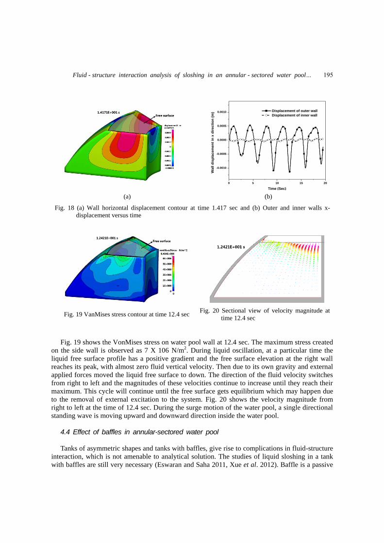
displacement histories of the container inner and outer walls are drawn in Figs. 18(a) and 18(b).

The Fig. 15 shows that the steady state values are reached from around 12 sec for 0.1 m

excitation amplitude. The displacement is captured at 12.04 sec. The displacement frequency is

almost equal to wave frequency. And it can be seen that the horizontal displacement is symmetric

in both side walls as shown in Fig. 18.

0 2 4 6 8 10 12 14 16

0

20

40

60

80

100

120 Position A

Position B

Position C

Position D

Position E

Pre

ssu

re (

Kp

a)

Time (Sec)

(a) (b)

Fig. 17 (a) Pressure point locations and (b) Time history of pressure at various locations for 0.1 m

amplitude sec and 1 =0.312 Hz

194


0 5 10 15 20

-0.0010

-0.0005

0.0000

0.0005

0.0010

Displacement of outer wall

Displacement of inner wall

Wall

dis

pla

cem

en

t in

x d

irecti

on

(m

)

Time (Sec)

(a) (b)

Fig. 18 (a) Wall horizontal displacement contour at time 1.417 sec and (b) Outer and inner walls x-

displacement versus time

Fig. 19 VanMises stress contour at time 12.4 sec Fig. 20 Sectional view of velocity magnitude at

time 12.4 sec

Fig. 19 shows the VonMises stress on water pool wall at 12.4 sec. The maximum stress created

on the side wall is observed as 7 X 106 N/m2. During liquid oscillation, at a particular time the

liquid free surface profile has a positive gradient and the free surface elevation at the right wall

reaches its peak, with almost zero fluid vertical velocity. Then due to its own gravity and external

applied forces moved the liquid free surface to down. The direction of the fluid velocity switches

from right to left and the magnitudes of these velocities continue to increase until they reach their

maximum. This cycle will continue until the free surface gets equilibrium which may happen due

to the removal of external excitation to the system. Fig. 20 shows the velocity magnitude from

right to left at the time of 12.4 sec. During the surge motion of the water pool, a single directional

standing wave is moving upward and downward direction inside the water pool.

4.4 Effect of baffles in annular-sectored water pool

Tanks of asymmetric shapes and tanks with baffles, give rise to complications in fluid-structure

interaction, which is not amenable to analytical solution. The studies of liquid sloshing in a tank

with baffles are still very necessary (Eswaran and Saha 2011, Xue et al. 2012). Baffle is a passive

195


device which reduces sloshing effects by dissipating kinetic energy due to the production of

vortices into the fluid. The linear sloshing in a circular cylindrical tank with rigid baffles is being

investigated by many authors in the context of spacecraft and ocean applications. The shapes and

positions need to be designed with the use of either numerical model or experimental approaches.

Nonetheless, the damping mechanisms of baffle are still not fully understood. The effects of baffle

on the free and forced vibration of liquid containers were studied by Gedikli and Erguven (1999),

Biswal et al. (2006). To the author‟s knowledge, there is a very limited set of analytically oriented

approaches to the sloshing problem in baffled tanks.

Here, two types of baffles are taken for analysis. First one is an annular baffle as depicted in

Figs. 21(a) and 21(b). Few authors worked on this annular baffle for their own geometries mainly

two dimensional. This article is focused on annular baffle for a three dimensional annular

cylindrical water pool. Biswal et al. (2006) found that the baffle has significant effect on the non-

linear slosh amplitude of liquid when placed close to the free surface of liquid. The effect is almost

negligible when the baffle is moved very close to the bottom of the tank. Past investigations also

convey that the performance of the annular baffle is better when it is near to the liquid free surface

(Eswaran et al. 2009). Second one is cap-plate baffle or shroud as shown in Figs. 21(c) and 21(d)

which is fixed at center of the water pool. (More details about baffle for thermal stratification can

be found in Vijayan 2010). Under reactor shutdown conditions, natural convection process starts

due to the strong heat source at the IC wall. Long time effect of this natural convection process

leads to warm fluid layers floating on the top of gradually colder layers. This results in a thermally

stratified pool having steep temperature gradient along the vertical plane. Over a period of time,

the substantial part of this pool gets thermally stratified except for the region close to the heat

source where there is horizontal temperature gradient as well (Gupta et al. 2009). Cap-plate model

has been proposed to satisfy the thermal stratification inside the water pool, since this water pool is

mainly designed to perform as a suppression pool to cool the steam and air mixture during LOCA

in the reactor vessel.

Annular Cap plate

Volume = 7.3 m3

Thickness = 200 mm

Height = 250 mm

Volume = 36 m3

Thickness = 200 mm

Height = 5 m

Annular Cap plate

Volume = 7.3 m3

Thickness = 200 mm

Height = 250 mm

Volume = 36 m3

Thickness = 200 mm

Height = 5 m

(a) Annular baffle (b) Annular baffle in the water pool. Annular Cap plate

Volume = 7.3 m3

Thickness = 200 mm

Height = 250 mm

Volume = 36 m3

Thickness = 200 mm

Height = 5 m

Annular Cap plate

Volume = 7.3 m3

Thickness = 200 mm

Height = 250 mm

Volume = 36 m3

Thickness = 200 mm

Height = 5 m

(c) Cap-plate baffle (d) Cap-plate baffle (or shroud) in the water pool

Fig. 21 Baffles shape and its position in the water pool

196


Liquid sloshing is violent near free surface and the liquid motion at the bottom of the tank is

almost zero. Here, one could assume that the mounting of the cap-plate does not disturb the liquid

sloshing as it is placed at bottom of the tank. The present work also estimate and compare the

annular and cap-plate baffle performance against the liquid sloshing under the regular excitation.

Fig. 22 illustrates that the comparison of liquid elevations for un-baffle, annular baffle and cap-

plate baffle cases. As expected, both the baffle cases reduce the liquid oscillations as well. It is

found that cap-plate baffle is more effective in reducing the sloshing oscillations and sloshing

pressure. To elucidate the performance of baffles, at near right corner the liquid height is captured

and shown in Fig. 23. The liquid height is captured near the right corner of water pool at 14.85 sec

under the excitation frequency ( 1 ) of 0.312 Hz. The liquid height deviation for no baffle case is

found at excitation amplitude between 0.01 m and 0.1 m is around 1.23 m. At the same time, this

value for annular baffle and cap - plate baffle is around 0.563 m and 0.182 m respectively.

Moreover, it is found from the numerical investigation that the liquid from the annular-sectored

water pool will spill out around 0.06 m excitation amplitude ( 0.023 g acceleration) under liquid

first mode frequency. The response spectrum for the structure will give us design acceleration

corresponding to first mode frequency. Here, design acceleration is 0.16 g at 0.312 Hz and

corresponds to 0.028 m equivalent harmonic amplitude. This line is shown as vertical in Fig. 23 to

mark free surface elevations for all cases. Baffle reduces the liquid slosh height 0.7 m to 0.3 m at

design acceleration. Now as shown in Fig. 23 the li The Fig. 24 is drawn for qualitative

comparison between no baffle, annular and cap-plate baffle case. Here, snap shots of liquid water

pool (under regular excitation of 0.1 m amplitude) for different time step has been shown.

0 5 10 15 20

-2

-1

0

1

2

No baffle

Annular baffle

Cap-plate baffle

(

m)

Time (Sec)

Fig. 22 Comparison of liquid elevations with no baffle, annular baffle and cap-plate baffle cases at

1 =0.312 Hz and amplitude 0.1 m

0.01 0.02 0.06 0.17.5

8.0

8.5

9.0

9.5

10.0

Line equivalent to design acceleration

Line of mean water level

Line of the top of the tank

Ma

xim

um

Liq

uid

He

igh

t (m

)

Excitation Amplitude (m)

No baffle with FSI

No baffle without FSI

Annular Baffle with FSI

Cap-plate Baffle with FSI

Fig. 23 Effect of baffles at right corner of the water pool case at 15.05 sec and 1 =0.312 Hz

197


(a) Time at 0 sec (e) Time at 0 sec (i) Time at 0 sec

(b) Time at 14.6 sec (f) Time at 14.6 sec (j) Time at 14.6 sec

(c) Time at 15.6 sec (g) Time at 15.6 sec (k) Time at 15.6 sec

(d) Time at 16.6 sec (h) Time at 16.6 sec (l) Time at 16.6 sec

Fig. 24 Comparisons of free surface profile at different time instant for un-baffled and baffled water pool

for 0.1 m amplitude sec and 1 =0.312 Hz. (Figs. (a)-(d), (e)-(h), (i)-(l) show un-baffled, annular

baffled, cap-plate baffled water pools respectively)

198


0 2 4 6 8 10 12 14 16

-1.2

-0.8

-0.4

0.0

0.4

0.8

1.2

(

m)

Time (Sec)

Annular Baffle

Cap-plate baffle

0 2 4 6 8 10 12 14 16

-2.0

-1.5

-1.0

-0.5

0.0

0.5

1.0

1.5

2.0

(

m)

Time (Sec)

Annular Baffle

Cap-plate Baffle

Fig. 25 Comparison of free surface elevation of

liquid at 0.1 m amplitude and 5 1

excitation frequency

Fig. 26 Comparison of free surface elevation of

liquid at 0.1 m amplitude and 10 1

excitation frequency

5. Conclusions

This work focused the numerical investigation on liquid sloshing in a three dimensional annular

water pool. Effect of baffles in the annular water pool is studied for different excitation and

amplitude. The effect of higher mode on the dynamic response of liquid containing structures is

also studied. If liquid oscillation is not controlled efficiently, sloshing of liquids in storage water

pools may lead to water spilled out from water pool or large dynamic stress to cause structural

failure. Hence, the study of sloshing and measures to suppress it are well justified with two types

of baffles for this kind of annular water pools. From the above numerical investigation, the

following observations are made.

(i) The liquid free surface elevation has been captured for different excitations and different

amplitudes. Since the liquid first mode frequency is very less than the structure first mode

frequency, the fluid-structure interaction effect is found to be negligible. As a result, the fluid

pressure on the free surface is dominated by the sloshing pressure or convective pressure and the

relative or fluid-structure interaction pressures are negligibly small for the case of first mode

excitation.

(ii) It is found from the numerical investigation that the liquid will spill out around 0.06 m

excitation amplitude ( 0.023 g acceleration) from the annular-sectored water pool under first

mode sloshing frequency. Design acceleration is 0.16 g at 0.312 Hz and corresponds to 0.028 m

equivalent harmonic amplitude. Baffle reduces the liquid slosh height 0.7 m to 0.3 m at design

acceleration.

(iii) As expected, annular baffle and cap-plate baffle cases are reducing the liquid oscillations as

well. However, cap-plate baffle is more effective in reducing the sloshing oscillations for this kind

of water pool geometries.

(iv) When the water pools are subjected to higher modes (i.e., higher than first mode excitation),

the fluid in the water pool will tend to undergo sloshing motions. In the higher modes the liquid

elevation is lower than the first mode frequency. At the beginning of the disturbance, the fluid

dynamic pressure is dominated by the impulsive pressure. After few seconds, sloshing pressure or

199


the convective pressure becomes the dominant component pressure.

This present work can be extended by investigating the liquid water pool under random

oscillations. And further, the during the accident conditions, the thermal stratification can be

expected due to the strong heat source from IC condensers which are immersed inside the water

pool. The heat transfer effect on the fluid sloshing can be studied under regular excitations and

random excitations of water pool.

References

Benra, F.K., Dohmen, H.J., Pei, J., Schuster, S. and Wan, B. (2011), “A comparison of one-way and two-

way coupling methods for numerical analysis of fluid-structure interactions”, J. Appl. Math., Article ID

853560.

Biswal, K.C., Bhattacharyya, S.K. and Sinha, P.K. (2006), “Non-linear sloshing in partially liquid filled

containers with baffles”, Int. J. Numer. Meth. Eng., 68(3), 317-337.

Chang, Y.W., Gvildys, J., Ma, D.C., Singer, R., Rodwell, E. and Sakurai, A. (1989), “Numerical simulation

of seismic sloshing of LMR reactors”, Nucl. Eng. Des., 113(3), 435-454.

Chen, B.F. and Nokes, R. (2005), “Time-independent finite difference analysis of 2D and nonlinear viscous

liquid sloshing in a rectangular tank”, J. Comput. Phys., 209(1), 47-81.

Chen, S., Johnson, D.B., Raad P.E. and Fadda, D. (1997), “The surface marker and micro cell method”, Int.

J. Numer. Meth. Fl., 25, 749-778.

ESI CFD Inc., CFD-ACE+, V2011.0, Modules Manual, Part 2, ESI-Group.

ESI US R&D, CFD-ACE (U)® (2011), User‟s Manual. Huntsville (AL, USA): ESI-CFD Inc.; 2011. (Web

site: www.esi-cfd.com).

Eswaran, M. and Saha, U.K. (2009), “Low steeping waves simulation in a vertical excited container using

sigma transformation”, Proceedings of the ASME 28th International Conference on Ocean, Offshore and

Arctic Engineering OMAE 2009, Hawaii, USA.

Eswaran, M. and Saha, U.K. (2010), “Wave simulation in an excited cylindrical tank using sigma

transformation”, Proceedings of the ASME International Mechanical Engineering Congress & Exposition,

Vancouver, BC, Canada.

Eswaran, M., Singh, A. and Saha, U.K. (2010), “Experimental measurement of the surface velocity field in

an externally induced sloshing tank”, J. Eng. Maritime Environ., 225(2), 133-148.

Eswaran M., and Saha UK. (2011), “Sloshing of liquids in partially filled tanks – A review of experimental

investigations”, International Journal of Ocean Systems Engineering, 1(2), 131-155.

Eswaran, M., Saha, U.K. and Maity, D. (2009), “Effect of baffles on a partially filled cubic tank: Numerical

simulation and experimental validation”, Comput. Struct., 87(3-4), 198-205.

Faltinsen, O.M., Rognebakke, O.F., Lukovsky, I.A. and Timokha, A.N. (2000), “Multidimensional modal

analysis of nonlinear sloshing in a rectangular tank with finite water depth”, J. Fluid Mech., 407, 201-234.

Frandsen, J.B. (2004), “Sloshing motions in excited tanks”, J. Comput. Physics 196(1), 53-87.

Gedikli, A. and Erguven, M.E. (1999), “Seismic analysis of a liquid storage tank with a baffle”, J. Sound

Vib., 223(1), 141-155.

Glatzel, T., Litterst, C., Cupelli, C., Lindemann, T., Moosmann, C., Niekrawietz, R., Streule, W., Zengerle,

R. and Koltay, P. (2008), “Computational fluid dynamics (CFD) software tools for microfluidic

applications – A case study”, Comput. Fluids, 37, 218-235.

Gupta, A., Eswaran, V., Munshi, P., Maheshwari, N.K. and Vijayan, P.K. (2009), “Thermal stratification

studies in a side heated water pool for advanced heavy water reactor applications”, Heat Mass Transfer,

45, 275-285.

Haroun, M.A. and Housner, G.W. (1981), “Seismic design of liquid storage tanks”, J. Tech. Council - ASCE,

107(1), 191-207.

Hirt, C.W. and Nichols, B.D. (1981), “Volume of fluid (VOF) method for the dynamics of free boundaries”,

200

http://www.esi-cfd.com/


J. Comput. Phys., 39(1), 201-25.

Lee, K., Lee K.H., Lee J.I., Jeong Y.H. and Lee P.S. (2013), “A new design concept for offshore nuclear

power plants with enhanced safety features”, Nucl. Eng. Des., 254, 129-141.

Ibrahim, R.A. (2005), Liquid sloshing dynamics: theory & applications, Cambridge University Press, New

York.

Kandasamy T., Rakheja S. and Ahmed, A.K.W. (2010), “An analysis of baffles designs for limiting fluid

slosh in partly filled tank trucks”, Open Transport. J., 4, 23-32.

Malhotra, P.K. (1997), “Seismic response of soil supported unanchored liquid storage tanks”, J. Struct. Eng.

- ASCE, 123(4), 440-450.

Sinha, R.K. and Kakodkar A. (2006), “Design and development of the AHWR- the Indian thorium fuelled

innovative nuclear reactor”, Nucl. Eng. Des., 236(7-8), 683-700.

Tedesco, J.W., Landis, D.W. and Kostem, C.N. (1989), “Seismic Analysis of cylindrical liquid storage

tanks”, Comput. Struct., 32(5), 1165-1174.

Vijayan, P.K. (2010), “Reducing thermal stratification and boiling in pools with immersed heat exchangers”,

Proceedings of the 3rd Meeting, 4-5 November 2010, IAEA Headquarters, Vienna, Austria

(www.iaea.org/INPRO/CPs/AWCR/3rd_Meeting/Indian-3-1.pdf ).

Vorobyev, A., Kriventsev, V. and Maschek, W. (2011), “Simulation of central sloshing experiments with

smoothed particle hydrodynamics (SPH) method”, Nucl. Eng. Des., 241, 3086-3096.

Xue, M.A., Zheng, J. and Lin, P. (2012), “Numerical simulation of sloshing phenomena in cubic tank with

multiple baffles”, J. Appl.Math., Article ID 245702.

201

http://www.iaea.org/INPRO/CPs/AWCR/3rd_Meeting/Indian-3-1.pdf

fluid–structure interaction analysis of sloshing in an

Documents