integration of fluid sloshing models with complex vehicle
TRANSCRIPT

Integration of Fluid Sloshing Models with Complex Vehicle System Algorithms
BY
BRYNNE E. NICOLSEN
B.Sc. in Bioengineering, University of Illinois at Chicago, 2015
THESIS
Submitted as partial fulfillment of the requirements
for the degree of Doctor of Philosophy in Mechanical Engineering
in the Graduate College of the
University of Illinois at Chicago, 2019
Chicago, Illinois
Defense Committee:
Professor Ahmed A. Shabana, Chair and Advisor, Mechanical and Industrial Engineering
Michael Brown, Mechanical and Industrial Engineering
Craig D. Foster, Civil and Materials Engineering
Thomas J. Royston, Bioengineering
James O’Shea, Exponent

ii
This thesis is dedicated to my family.

iii
ACKNOWLEDGEMENTS
I would like to thank my advisor, Dr. Ahmed Shabana, for his continued guidance and
encouragement during my studies. I am grateful for the opportunities he has provided me, and for
pushing me to never settle for less than my best effort. I would also like to thank the members of
my thesis committee: Dr. Michael Brown, Dr. Craig Foster, Dr. Thomas Royston, and Dr. James
O’Shea, for reviewing my work and providing valuable feedback. I am also grateful to Dr. Antonio
Recuero and Dr. Liang Wang for their invaluable assistance and encouragement when I first joined
the Dynamic Simulation Laboratory and had much to learn.
I would like to acknowledge the financial support of the National Science Foundation,
without which focusing on my research would have been much more difficult.
I would also like to thank my friends and colleagues in the Dynamic Simulation Laboratory
with whom I worked over several years, including Mohil Patel, Shubhankar Kulkarni, and
Emanuele Grossi. Each has contributed to my growth and education, through direct assistance and
informative discussions. I am also grateful to my internship supervisors at Navistar, Inc., Stefano
Cassara and Dr. Brendan Chan, for providing me with the opportunity to gain hands-on experience
learning about vehicle dynamics and working in an industry setting. Finally, I would like to thank
my family for teaching me to view the world from a scientific perspective and for providing me
with an upbringing that allowed me to pursue my dreams, and my fiancé Brian Tinsley, whose
support and encouragement were invaluable during my most difficult times.

iv
CONTRIBUTIONS OF THE AUTHORS
Chapter 2 represents a published manuscript (Nicolsen et al., 2017). My research advisor, Dr.
Ahmed A. Shabana, contributed to the review of this manuscript and guidance of the work. My
colleague, Dr. Liang Wang, contributed to developing the fluid constitutive model, the fluid-tank
contact model, and guidance of the work. I contributed to developing the vehicle model, the
numerical simulations, the tire/ground and fluid/tank contact models, and writing the manuscript.
Chapter 3 represents a published manuscript (Shi et al., 2017). My research advisor, Dr. Ahmed
A. Shabana, contributed to the review of this manuscript and guidance of the work. My colleagues,
Dr. Huailong Shi and Dr. Liang Wang, contributed to developing the fluid constitutive model, the
fluid/tank contact model, the numerical simulations, and writing the manuscript. I contributed to
the numerical simulations, the fluid/tank contact model, and writing the manuscript. Chapter 4
represents work that is not yet published. My research advisor, Dr. Ahmed A. Shabana, contributed
to review of this manuscript and guidance of the work. I contributed to developing the models, the
numerical simulations, and writing the manuscript.

v
TABLE OF CONTENTS
1. INTRODUCTION................................................................................................................... 1
1.1 Fluid Sloshing Phenomenon in Freight Transport .............................................................. 2
1.2 Fluid Modeling Techniques ................................................................................................ 4
1.3 Electronically-Coupled Pneumatic (ECP) Braking ............................................................. 7
1.4 Geometrically-Accurate ANCF/FFR Finite Elements ........................................................ 8
1.5 Scope and Organization of the Thesis ................................................................................. 9
2. FLUID MODELING WITH HIGHWAY VEHICLE APPLICATIONS ........................ 15
2.1. Basic Force Concepts ....................................................................................................... 16
2.2. Continuum-Based Inertia Force Definitions .................................................................... 19
2.3. ANCF Description of the Fluid Geometry ....................................................................... 22
2.4. ANCF Fluid Constitutive Model ...................................................................................... 25
2.5. Fluid-Tank Interaction...................................................................................................... 29
2.6. Vehicle Model Components ............................................................................................. 31
2.7. Specified Motion Trajectories .......................................................................................... 38
2.8. Equations of Motion ......................................................................................................... 41
2.9. Numerical Results ............................................................................................................ 42
2.10. Concluding Remarks ....................................................................................................... 55
3. FLUID MODELING WITH RAILROAD VEHICLE APPLICATIONS ....................... 58
3.1. Basic Inertia Force Definitions ........................................................................................ 59
3.2. Integration of Geometry and Analysis for Railroad Sloshing .......................................... 63
3.3. Fluid/Tank Interaction Forces .......................................................................................... 70
3.4. ANCF Fluid Constitutive Equations ................................................................................ 74
3.5. Integration with MBS Railroad Vehicle Algorithms ....................................................... 78
3.6. Numerical Simulations ..................................................................................................... 83
3.7. Concluding Remarks ........................................................................................................ 97
4. GEOMETRICALLY ACCURATE REDUCED ORDER FLUID MODELS ................ 99
4.1. FE Mesh Geometry and Position Vector Gradients ....................................................... 100
4.2. Finite Element Formulations .......................................................................................... 103
4.3. Fluid Modeling Approaches ........................................................................................... 109
4.4. Fluid/Tank Contact ......................................................................................................... 111

vi
TABLE OF CONTENTS (continued)
4.5. Equations of Motion ....................................................................................................... 114
4.6. Numerical Examples ...................................................................................................... 115
4.7. Concluding Remarks ...................................................................................................... 125
5. SUMMARY AND CONCLUSIONS ................................................................................. 127
6. APPENDIX A ...................................................................................................................... 132
7. APPENDIX B ...................................................................................................................... 134
8. APPENDIX C ...................................................................................................................... 136
9. REFERENCES .................................................................................................................... 138
10. VITA..................................................................................................................................... 147

vii
LIST OF TABLES
TABLE 1.1. ECONOMIC CHARACTERSTICS OF THE TRANSPORTATION INDUSTRY
IN 2007 ............................................................................................................................................2
TABLE 1.2. FREIGHT TONNAGE IN 2007 .................................................................................3
TABLE 2.1. MBS MODEL INERTIAL PROPERTIES ...............................................................32
TABLE 2.2. SUSPENSION PARAMETERS ...............................................................................38
TABLE 2.3. INITIAL VELOCITIES ............................................................................................42
TABLE 3.1. TRACK GEOMETRY ..............................................................................................80
TABLE 4.1. SLOSHING BOX MODEL INFORMATION .......................................................116
TABLE 4.2. REFERENCE CONDITIONS ................................................................................117
TABLE 4.3. NORMALIZED VEHICLE MODEL CPU TIMES ...............................................124
viii
LIST OF FIGURES
Figure 2.1. Force diagrams of a vehicle during (a) straight-line motion and (b) curve negotiation
........................................................................................................................................................16
Figure 2.2. Change in tire contact force during curve negotiation: (a) theoretical values, (b)
simulation results ...........................................................................................................................17
Figure 2.3. Tank geometry .............................................................................................................22
Figure 2.4. Initially curved fluid geometry ....................................................................................24
Figure 2.5. ANCF fluid mesh ........................................................................................................25
Figure 2.6. Fluid configurations.....................................................................................................26
Figure 2.7. Fluid-tank interaction in the (a) radial and (b) longitudinal direction .........................30
Figure 2.8. Brush Tire model coordinate systems .........................................................................34
Figure 2.9. Ackermann steering mechanism ..................................................................................36
Figure 2.10. Steering mechanism geometry ..................................................................................37
Figure 2.11. Trajectory constraint coordinate systems ..................................................................39
Figure 2.12. Commercial medium-duty tanker truck model ..........................................................42
Figure 2.13. Velocity during braking .............................................................................................43
Figure 2.14. Fluid sloshing due to braking ....................................................................................44
Figure 2.15. Normal force on a front tire and a rear tire during braking .......................................44
Figure 2.16. Position of fluid center of mass relative to tank during braking ...............................45
Figure 2.17. Flat free surface at steady state after braking ............................................................46
Figure 2.18. Lane change trajectory ..............................................................................................46
Figure 2.19. Lateral sloshing due to lane change maneuver ..........................................................48
Figure 2.20. Normal force on (a) a left-hand tire and (b) a right-hand tire during a lane change .48

ix
LIST OF FIGURES (continued)
Figure 2.21. Position of fluid center of mass relative to tank during lane change.........................49
Figure 2.22. Lateral friction force on (a) a left-hand tire and (b) a right-hand tire during a lane
change ............................................................................................................................................49
Figure 2.23. Lateral slip velocity on a left-hand tire during a lane change ...................................50
Figure 2.24. Curve trajectory .........................................................................................................51
Figure 2.25. Normal force on an outer tire and an inner tire during curve negotiation .................52
Figure 2.26. Lateral friction force on (a) an outer tire and (b) an inner tire during curve negotiation
........................................................................................................................................................52
Figure 2.27. Outward inertia force on fluid during curve negotiation ...........................................54
Figure 2.28. Position of fluid center of mass relative to tank during curve negotiation ................54
Figure 2.29. Normalized velocity of the fluid center of mass in the (a) longitudinal and (b) lateral
and vertical directions ....................................................................................................................55
Figure 3.1. A planar flexible body negotiating a curve ..................................................................61
Figure 3.2. Wheel/rail contact ........................................................................................................64
Figure 3.3. Curved ANCF rail element ..........................................................................................66
Figure 3.4. Fluid and tank geometry ..............................................................................................66
Figure 3.5. Cross-section mesh of the fluid inside a cylindrical tank ............................................67
Figure 3.6. ANCF solid element in the (a) curved reference and (b) straight configurations .......68
Figure 3.7. Initially curved ANCF fluid mesh ...............................................................................39
Figure 3.8. Tank geometry and coordinate systems ......................................................................71
Figure 3.9. Railroad vehicle model ................................................................................................79
Figure 3.10. Flowchart of the numerical solution procedure .........................................................84

x
LIST OF FIGURES (continued)
Figure 3.11. Lateral component of gravity and outward inertia forces of the fluid .......................86
Figure 3.12. Position of the tank center with respect to the track in the lateral direction at (a)
40km/h, (b) 60 km/h, and (c) 90 km/h ...........................................................................................87
Figure 3.13. Tangential component of fluid gravity and inertia forces at 40 km/h .......................88
Figure 3.14. Liquid center of mass with respect to the tank in the longitudinal direction ............89
Figure 3.15. Tread normal contact force of truck lead wheelset (a) 40km/h, (b) 60 km/h, (c) 90
km/h ...............................................................................................................................................90
Figure 3.16. Flange normal contact force of truck lead wheelset (a) 40km/h, (b) 60 km/h, (c) 90
km/h ...............................................................................................................................................91
Figure 3.17. Tread lateral contact force of lead wheelset of lead truck (a) 40km/h, (b) 60 km/h, (c)
90 km/h ..........................................................................................................................................92
Figure 3.18. Flange lateral contact force of lead wheelset of lead truck (a) 40km/h, (b) 60 km/h,
(c) 90 km/h .....................................................................................................................................92
Figure 3.19. Average normal contact forces of lead and rear trucks in the traction case ...............93
Figure 3.20. Fluid center of mass longitudinal displacement with respect to the tank in the traction
case .................................................................................................................................................94
Figure 3.21. Coupler forces between two cars in the case of braking using (a) Conventional brake,
(b) ECP brake .................................................................................................................................94
Figure 3.22. Front car fluid center of mass displacement with respect to the tank during braking (a)
Longitudinal, (b) Lateral direction .................................................................................................96
Figure 3.23. Braking animation of two tank-cars filled with liquid in the (a) Parked state, (b)
Braking state ..................................................................................................................................96

xi
LIST OF FIGURES (continued)
Figure 4.1. Cylindrical vehicle tank .............................................................................................100
Figure 4.2. Fluid configurations...................................................................................................101
Figure 4.3. Floating Frame of Reference formulation .................................................................106
Figure 4.4. Box boundary conditions ...........................................................................................117
Figure 4.5. Maximum deformation of most refined (a) ANCF and (b) ANCF/FFR fluid meshes
......................................................................................................................................................118
Figure 4.6. Vertical corner node position of (a) ANCF meshes and (b) ANCF/FFR meshes .....119
Figure 4.7. Normalized CPU times for the sloshing box models ................................................120
Figure 4.8. Medium-duty tanker truck MBS model ....................................................................120
Figure 4.9. Lane change path .......................................................................................................121
Figure 4.10. Lateral position of fluid center of mass with respect to tank during lane change
maneuver ......................................................................................................................................122
Figure 4.11. (a) Normal force on (a) a left-hand tire and (b) a right-hand tire during a lane change
......................................................................................................................................................123
Figure 4.12. (a) Lateral friction force on (a) a left-hand tire and (b) a right-hand tire during a lane
change ..........................................................................................................................................124

xii
SUMMARY
A new continuum-based total-Lagrangian liquid sloshing approach that accounts for the effect of
complex fluid and tank geometry on highway and railroad vehicle dynamics is developed in this
thesis. A unified geometry/analysis mesh is used from the outset to examine the effect of liquid
sloshing on vehicle dynamics during curve negotiation and braking, including electronically
controlled pneumatic (ECP) brakes. ECP brakes produce braking forces uniformly and
simultaneously across all railroad cars and are employed in order to reduce stopping distances and
coupler forces. In these motion scenarios, the liquid experiences large displacements and
significant changes in shape that can be captured effectively using the finite element (FE) absolute
nodal coordinate formulation (ANCF). ANCF-FEs can describe complex mesh geometries and
the change in inertia due to the change in the fluid shape, allowing for accurately capturing the
effect of the sloshing forces during motion scenarios.
The liquid sloshing models are integrated with three-dimensional multibody system (MBS)
highway and railroad vehicle algorithms which account for the nonlinear tire/ground and
wheel/rail contact. The three-dimensional contact force formulations used in this thesis account
for the longitudinal, lateral, and spin forces that influence the vehicle stability. A continuum-based
fluid constitutive model is employed, and a penalty-based fluid-tank contact algorithm is
developed. In order to examine the effect of the liquid sloshing on the vehicle dynamics during
curve negotiation, a general and precise definition of the outward inertia force is defined, which
for flexible bodies does not take the simple form used in rigid body dynamics. Specified motion
trajectories are used to examine the vehicle dynamics in different scenarios including deceleration
during straight-line motion, rapid lane change, and curve negotiation. The balance speed and

xiii
SUMMARY (continued)
centrifugal effects in the case of a railroad tank-car partially filled with liquid are studied and
compared with an equivalent rigid body model during curve negotiation and braking scenarios. In
particular, the results obtained in the case of the ECP brake application of two railroad freight car
model are compared with the results obtained when using conventional braking. The highway
vehicle tire contact forces are investigated and the effects of fluid sloshing on the vehicle stability
are demonstrated.
Lastly, for the first time the newly developed absolute nodal coordinate
formulation/floating frame of reference (ANCF/FFR) solid FEs are integrated with a fully
nonlinear MBS algorithm. ANCF/FFR-FEs are able to capture initially curved structures such as
the fluid within a cylindrical tank while retaining the same number of degrees of freedom as
conventional elements and taking advantage of modal reduction techniques, resulting in faster
simulation times compared to the higher-order ANCF elements. The solid element is developed in
terms of constant geometric coefficients which are obtained using the matrix of position vector
gradients defined in the reference configuration. No geometry distortion occurs when computer-
aided design (CAD) models are converted to FE meshes using ANCF/FFR elements because such
meshes are developed using ANCF elements, which are related to B-splines and Non-Uniform
Rational B-Splines (NURBS) by a linear mapping. The fluid constitutive model, which is based
on the Navier-Stokes fluid model, is developed and the incompressibility conditions, which are
enforced using a penalty approach, are defined. A sloshing box model and a medium-duty tanker
truck model with a tank half filled with water are developed in order to investigate the ability of
the new ANCF/FFR elements to model the fluid sloshing in comparison to fluid meshed using
ANCF elements. The fluid/tank contact formulation, which is enforced using a penalty approach,

xiv
SUMMARY (continued)
is described. It is shown that while the sloshing amplitudes of the ANCF/FFR box meshes are
reduced compared to the converged ANCF meshes, the general sloshing behavior is still captured
at a significantly reduced CPU time, indicating that the ANCF/FFR elements can contribute to
significant improvement of the computational efficiency in applications in which capturing some
geometric changes due to the fluid displacement is not critical. This conclusion is confirmed by
the results of the highway vehicle lane change simulation – the sloshing amplitudes of the center
of mass predicted using the ANCF/FFR fluid mesh during the lane change are found to be in a
good agreement with what predicted by the ANCF mesh. Furthermore, the results of the overall
vehicle-dynamics, as measured by the tire contact forces predicted using the two different meshes,
are found to be in a good agreement. The results obtained demonstrate that if the goal is to
accurately capture the free-surface displacement of the fluid, then ANCF elements are better
candidates due to their high order and ability to capture complex shapes. However, if the goal is
to perform efficient simulations to obtain the overall vehicle motion, then using ANCF/FFR
elements are a better alternative.

1
CHAPTER 1
INTRODUCTION
Fluid sloshing is the motion of a liquid in a container subjected to forced oscillations and occurs
in a moving container which is not fully filled. One industry which is significantly affected by
fluid sloshing is freight transportation – an increase in demand for crude oil and other hazardous
materials (HAZMAT) has in turn increased the number of highway and railroad vehicles
transporting these materials. Fluid sloshing can have a significant effect on vehicle dynamics,
especially in curve negotiation and traction and braking scenarios. It is clear that thorough
understanding of this complex phenomenon is necessary in order to design safe and reliable
vehicles. While many approaches have been used to model fluid sloshing, such as discrete inertia,
discrete element, and computational fluid dynamics models, each has drawbacks which limit its
scope of application. Finite element analysis (FEA), however, addresses many of these
shortcomings by using a general, physics-based approach. One objective of this thesis is to
integrate high-fidelity finite element (FE) fluid sloshing models with complex multibody system
(MBS) highway and railroad vehicle algorithms in order to study the effect of fluid sloshing on
vehicle dynamics and stability. Additionally, the effect of fluid sloshing on the coupler forces of
railroad vehicles during braking scenarios will be investigated, including the efficacy of
electronically-controlled pneumatic brakes. The standard definition for the centrifugal force will
also be assessed and it will be shown that it is inadequate for describing the outward inertia forces
of flexible bodies. Finally, fluid sloshing models based on two different FE formulations will be
compared in order to assess their ability and efficiency in accurately capturing the fluid sloshing
phenomenon.

2
1.1. Fluid Sloshing Phenomenon in Freight Transport
The field of fluid dynamics has been extensively studied for decades using, for the most part,
Eulerian approaches. Another area of application that has recently seen significant advances is
vehicle dynamics, which is often examined using MBS algorithms based on a total Lagrangian
approach. Nonetheless, fluid-vehicle interaction impacts many areas of science and technology
including rail, highway, aerospace, and marine transportation. Although materials, including crude
oil and other HAZMAT, are transported using a variety of methods, including shipping vessels
and pipelines, transportation by highway vehicle dominates the industry, generating more revenue
and creating more jobs than the other modes of transportation combined, as shown by the data
presented in Table 1.1. Due to the extent of public roads in the US and the sheer volume of freight
vehicles, the tonnage of materials transported using highway vehicles far outweighs all other
methods. This is true for both non-hazardous and hazardous materials, as shown in Table 1.2 (U.S.
Department of Transportation, 2011).
Table 1.1. Economic characteristics of the transportation industry in 2007 (U.S. Department of
Transportation, 2011)
Mode Establishments Revenue (millions) Paid Employees
Highway 120,390 217,833 1,507,923
Railway* 563 49,400 169,891
Waterway 1,721 34,447 75,997
Pipeline 2,529 25,718 36,964
*Data for Railway are for 2009.
Rollovers are more common in tanker trucks than passenger vehicles because trucks have
a higher center of gravity. Rollovers can occur due to a variety of reasons, including vehicle and
road conditions, load size, and the most common, driver error, which accounts for up to 78% of
tanker truck rollovers (U.S. Department of Transportation, 2007). Hazardous materials are

3
regularly transported by tanker trucks, and accidents in which the tank is compromised and the
contents are released can lead to damage to the environment and the surrounding infrastructure,
fires and explosions, and civilian injuries and casualties (Shen et al., 2014; WSB-TV 2015). In
the last decade alone, highway transportation accidents comprised the majority of all HAZMAT
incidents, with 144,296 out of a total of 166,494 incidents; other incidents include air, railway, and
water transportation accidents. Highway accidents have also proven to be the most deadly and
costly, accounting for 100 out of 105 documented fatalities and 1,520 out of 2,129 injuries, at a
cost of $6.1 billion out of $8.2 billion in damages (U.S. Department of Transportation, PHMSA,
2015). Therefore, thorough testing and virtual prototyping are necessary to ensure better vehicle
design and stability. However, because physical prototyping is expensive, inefficient, and time-
consuming, it is necessary to develop accurate predictive models to investigate the effect of liquid
sloshing on the dynamics of highway vehicles subject to different loading conditions and motion
scenarios.
Table 1.2. Freight tonnage in 2007 (U.S. Department of Transportation, 2011)
Mode Hazardous Materials Non-Hazardous Materials Total Tons
(Thousands) Tons
(Thousands)
Percentage
of Mode
Tons
(Thousands)
Percentage
of Mode
Highway 1,202,825 14 7,575,888 86 8,778,713
Railway 129,743 7 1,731,564 93 1,861,307
Waterway 149,794 37 253,845 63 403,639
Pipeline 628,905 97 21,954 3 650,859
Air 362 10 3,256 90 3,618
As shown in Table 1.2, railroad vehicles are the second most common mode of
transportation of freight materials. The high demand of crude oil and other HAZMAT
transportation has resulted in many serious and environmentally-damaging highway and railroad

4
accidents (King and Trichur, 2015; Wronski, 2013). In railroad transportation, liquid sloshing can
have a significant effect on railroad vehicle dynamics, especially in curve negotiation and traction
and braking scenarios (Vera et al., 2005; Wang et al., 2014). Although statistics show that most of
the accidents were caused by misuse or careless driving by the operator, extensive mathematical
and empirical studies must be performed to examine the effect of liquid sloshing on vehicle
dynamics and stability.
1.2. Fluid Modeling Techniques
Although recent advances allow for modeling more accurate fluid behavior, most commonly used
models are insufficient in adequately capturing the dynamics of the fluid in complex motion
scenarios, particularly in the cases of three-dimensional finite rigid body rotations. Early sloshing
models represented the fluid as a series of planar pendulums or mass-spring systems (Graham,
1951; Graham and Rodriguez, 1952; Abramson, 1966; Zheng et al., 2012); spherical and
compound pendulums were later used to capture nonlinearities in the motion and damping was
added to include the effect of energy dissipation (Ranganathan et al., 1989). Discrete inertia models
have been used extensively in studying sloshing dynamics in the aerospace industry since the
1960s (Abramson, 1966; Cui et al., 2014; Nichkawde et al., 2004). Coefficients for these
equivalent mechanical models can be obtained from experimental results, or using potential flow
solutions (Dodge, 2000). However, while these discrete inertia models have been improved over
time, such models cannot be used to accurately capture the change in inertia due to a change in
fluid shape and the complex dynamics that results from the vehicle motion (Liu and Liu, 2010).
Furthermore, the discrete rigid body models do not allow for modeling the continuous free surface
of the fluid, and it has been found that while the solution of a pendulum system agreed well with
5
a computational fluid dynamics (CFD) model for tanks with low fill levels, increasing the fill level
resulted in underprediction of the sloshing amplitudes and forces. Tank models with low fill levels
are relevant to aerospace applications and contribute to better understanding of the vehicle
behavior during low-fuel scenarios; however, for highway and railroad vehicles it is desirable to
transport the cargo at maximum capacity in order to reduce the sloshing behavior and maximize
transportation efficiency, so discrete inertia models are not suitable for studying such systems.
The discrete element method (DEM), in which the fluid is modeled as a system of small
particles, has also been used to study fluid sloshing (Cundall and Strack, 1979). DEM has the
advantage of capturing the mixing of different fluids and is thus often used in multi-phase
simulations (Monaghan, 2012; Nishiura et al., 2014). DEM is also capable of capturing fluid
separation and is therefore an important tool in studying fluid-structure interaction (Boffi and
Gastaldi, 2016; Pingle et al., 2012). However, while torsional motion and fluid separation are
important for systems such as multi-phase flow and fluid-structure interaction, these phenomena
do not significantly affect the overall vehicle dynamics. Furthermore, DEM models often suffer
from very high problem dimensionality, particularly in the case of vehicle tanks with cargo in
excess of several thousand gallons – for example, 15,000-gallon cargo is common in the case of a
rail tank-car. A large tank volume requires millions of particles to accurately capture the sloshing
behavior, which significantly increases the computation cost. Thus, DEM models are also not
optimal for studying sloshing dynamics in vehicle applications.
The governing equations of fluid dynamics, including conservation of mass and
momentum, are in general highly nonlinear coupled differential equations, and a closed-form
analytical solution does not exist. Computational fluid dynamics (CFD) is a numerical approach
for solving the fluid equations, where the fluid volume is divided into many control volumes over

6
which the partial differential equations are converted to discrete equations which can be solved
iteratively (Griffiths and Boysan, 1996). There are several commercially-available CFD solvers
such as ANSYS Fluent (ANSYS, 2019). Eulerian-based CFD solvers are commonly used by the
fluid dynamics community due to the Eulerian nature of many current problems of interest.
However, many MBS algorithms are based on a Lagrangian formulation, and integration with
Eulerian CFD solvers has been shown to be problematic. Fluid sloshing is often studied in fixed
containers which are subjected to forced excitation, so Eulerian approaches are suitable. Practically,
however, fluid sloshing often occurs in dynamic systems, such as rockets and highway and railroad
vehicles, resulting in highly nonlinear centrifugal and Coriolis forces which are not captured using
existing CFD models. Thus, in order to use the CFD approach to study a complex mechanical
system, it would be necessary to combine an Eulerian fluid sloshing problem with a Lagrangian
MBS algorithm. Pape et al. (2016) attempted to integrate a CFD model with the commercial
vehicle-dynamics software TruckSim, but due to the incompatible nature of the two solvers,
integration was found to be impossible and a discrete inertia model was instead used. It is due to
this incompatibility that CFD models are not suitable for studying fluid sloshing in complex
mechanical systems. Furthermore, modeling the fluid free surface is also challenging using
Eulerian methods.
In the case of liquid sloshing problems, accurate definition of the geometry of the fluid and
container is necessary in order to develop a general computational framework that can be
effectively used to shed light on the effect of sloshing in complex motion scenarios. In order to
take advantage of the Lagrangian nature of existing MBS algorithms, a number of continuum-
based fluid models have been developed. Wang et al. (2015) developed a low-order fluid sloshing
model based on the FE/FFR formulation. The FE/FFR formulation uses a modal approach to

7
reduce significantly the problem dimensionality. The numerical results obtained using a railroad
vehicle model showed that while an increase in the fluid viscosity improves the stability at low
velocities due to the damping effect, at high velocities the increase in the fluid viscosity leads to
an increase in the vehicle hunting oscillations when compared to an equivalent rigid-body fluid
model. However, because the small-deformation FFR elements may not be capable of showing
severe sloshing behavior, Wei et al. (2015) developed a total-Lagrangian ANCF sloshing model.
This non-modal, non-incremental approach leads to a constant mass matrix and zero Coriolis and
centrifugal forces. It was shown that a single ANCF element can capture much more severe
deformation compared to a large number of conventional FFR elements. The FFR and ANCF
approaches are both fully Lagrangian and thus can be easily integrated with existing MBS
algorithms.
1.3. Electronically-Coupled Pneumatic (ECP) Braking
The coupler is a device which is used to connect two railcars. In the case of sudden braking,
excessive coupler forces can be generated between the railcars, which can be exacerbated by fluid
sloshing. These forces can cause damage to the couplers, which can shorten their lifespans and
require premature replacement. Failure of the coupler can also allow the railcars to separate, which
can lead to runaway cars, collisions, or derailment. The purpose of the newly introduced
electronically controlled pneumatic (ECP) braking system, recommended for long freight trains,
is to apply the braking forces uniformly and simultaneously on all railcars. This new technology
can improve both train safety and operations by reducing the coupler forces and decreasing
stopping distances. Studies have shown that the ECP braking system, as compared to conventional

8
braking, leads to a 40% reduction in the stopping distance and significant reduction in the coupler
forces (Aboubakr et al., 2016).
1.4. Geometrically-Accurate ANCF/FFR Finite Elements
Recently a new class of elements which can model initially curved structures and also allow for
using modal reduction techniques has been proposed (Shabana, 2017B). These elements, referred
to as ANCF/FFR elements, are based on the ANCF kinematic description and are thus able to
capture initially curved geometry in the reference configuration, such as fluid within a tank, tires,
and leaf springs. The position vector gradients which define the initially curved geometry of the
mesh are written in terms of finite rotations by use of a consistent rotation-based formulation
(CRBF) velocity transformation matrix, thus allowing for the development of reduced-order
models which can be used in both structural and MBS applications. Furthermore, because ANCF
elements are related to B-splines and Non-Uniform Rational B-Splines (NURBS) by a simple
linear mapping, conversion from CAD geometry to analysis meshes is a straightforward process
which avoids distortion of the mesh. Conventional finite elements are not related to CAD models
by a linear mapping, and consequently, conversion to FE meshes is a much more costly and error-
prone process, costing the U.S. automotive industry alone over $600m in 2011 (Mackenzie, 2012).
The convergence of ANCF/FFR element frequencies has been shown to agree well with
commercial FE software for simple geometries (Zhang et al., 2019; Tinsley and Shabana, 2019),
but the performance of these elements has not yet been evaluated in the case of full vehicle models
or compared to ANCF elements.

9
1.5. Scope and Organization of the Thesis
Chapter 2 was first published in the Journal of Sound and Vibration (Nicolsen et al., 2017) and is
reproduced in this thesis with permission, which is provided in Appendix A. In this chapter, a
formulation that correctly captures the geometry of the fluid and tank is used in order to accurately
represent the distributed inertia and elasticity of the fluid. In order to develop these new and unique
sloshing geometry models, ANCF elements that produce accurate geometry are used, eliminating
the need for using B-spline and NURBS representations for developing the complex fluid
geometry. The effect of the initially curved fluid geometry, which cannot be captured accurately
using existing FE formulations, is properly accounted for, leading to a systematic integration of
the geometry and analysis by adopting one fluid mesh from the outset. Such an important goal
cannot be achieved using other MBS formulations that employ modal representation for the fluid
displacements, as in the case of the FFR formulation (Wang et al., 2014).
The ANCF geometry/analysis mesh developed is used to formulate the inertia forces using
a non-modal continuum-based approach. Proper definition of the inertia forces is necessary in
order to be able to predict the effect of the sloshing on the vehicle dynamics and stability. In
particular, a continuum-based and general definition of the centrifugal forces in terms of the fluid
displacement is developed and used to shed light on the approximation made using the simple rigid
body dynamics formula 2
smV r . Accurate definition of the centrifugal forces is particularly
important in the definition of the vehicle balance speed that should not be exceeded during curve
negotiations. An ANCF fluid/tank car walls penalty contact formulation is developed and used to
determine the generalized contact forces associated with the ANCF nodal coordinates which
include absolute position and gradient vectors. The penalty contact formulation developed in this

10
chapter takes into account the fluid large displacement and complex geometry that result from the
sloshing effect.
It is shown in this chapter how general constitutive fluid models can be developed and
integrated with ANCF complex fluid geometry models, thereby opening the door for future
investigations that focus on adopting new and highly nonlinear constitutive fluid models as well
as experimenting with different tank designs that have different, complex, and unconventional
geometries. In so doing, the field of liquid sloshing can be significantly advanced to a new level.
The analysis presented in this chapter demonstrates for the first time how an ANCF liquid
sloshing model can be integrated with an MBS system computational algorithm that ensures that
the kinematic algebraic constraint equations are satisfied at the position, velocity, and acceleration
levels. Such new ANCF fluid/MBS algorithms will allow for investigating a large class of liquid
sloshing problems that cannot be solved using existing approaches. The purpose of this analysis is
to create a high-fidelity model which is capable of capturing more details than can be described by
existing modeling methods. It is important to note that simple models can still be valuable if real-
time simulations are required. In these cases, both simple vehicle and fluid models can be used to
significantly reduce the computer simulation time. High fidelity continuum-based models, on the
other hand, are necessary in order to account for the distributed inertia and viscoelasticity of the
fluid.
The use of the formulation and computational procedure developed in this chapter is
demonstrated using a fully nonlinear MBS model of a commercial medium-duty tanker truck
developed using the general-purpose MBS software SIGMA/SAMS (Systematic Integration of
Geometric Modeling and Analysis for the Simulation of Articulated Mechanical Systems). The
fluid in the tank is represented by an ANCF mesh which allows for capturing the change in inertia
11
due to the change in shape of the fluid, as well as visualizing the change in the fluid free surface
while correctly capturing the centrifugal forces. The interaction between the rigid tank walls and
the ANCF fluid is formulated using the penalty approach. The MBS model includes a suspension
system and Pacejka’s brush tire model is introduced to represent the ground-tire contact (Pacejka,
2006). Specified motion trajectories are used to examine three different working conditions –
deceleration under straight-line motion, rapid lane changing, and negotiating a curve. Reduced
integration is used to increase computational efficiency when the fluid viscosity forces are
calculated. The results show that sloshing has the effect of increasing contact forces on some
wheels and decreasing contact forces on other wheels. Severe sloshing behavior can cause vehicle
instability; in extreme cases, wheel lift and vehicle rollover may occur.
Chapter 3 was first published in the Journal of Multi-Body Dynamics (Shi et al., 2017)
and is reproduced in this thesis with permission, which is provided in Appendix B. In this chapter,
the computational continuum-based total Lagrangian approach is used to study the effect of liquid
sloshing on railroad vehicle dynamics during curve negotiation and braking scenarios. A unified
geometry/analysis mesh (Cottrell et al., 2007; Shabana 2017) is used from the outset to define the
tank-car and fluid configuration, demonstrating a successful integration of computer aided-design
and analysis (I-CAD-A) for an important and practical problem. The general definition of the
liquid outward inertia forces, which is fundamentally different from the case of rigid body
dynamics, is defined in this chapter using the FFR formulation, and it is shown that the
conventional centrifugal force definition used to define the vehicle balance speed during curve
negotiations is a special case of the more general expression. The geometry description of both the
tank and the fluid using ANCF elements is discussed, and it is shown how ANCF elements can be
used with cubic spline function representation to define the geometry of the rigid rails. The

12
formulation of the liquid/tank interaction forces and the search method used to define the fluid/tank
contact points are described and the constitutive fluid model used in the total Lagrangian and non-
incremental solution procedure adopted in this paper is briefly discussed. The integration of the
liquid sloshing model in computational MBS railroad vehicle algorithms, the track geometry, and
the three-dimensional wheel/rail contact force model are elaborated. The components of the MBS
vehicle model and the fluid model data used to examine the effect of liquid sloshing on the
performance of the newly introduced ECP brake system and the rail vehicle dynamics during curve
negotiations are also detailed. In this chapter, the results obtained using the ECP braking force
model are compared with the results obtained using the conventional air brake system. In order to
improve the efficiency of the simulation, integration techniques such as the Hilber-Hughes-Taylor
(HHT) method (Aboubakr et al., 2015) and reduced integration when calculating the fluid viscous
forces are used.
Chapter 4 presents a general procedure which can be used to develop geometrically
accurate spatial finite elements capable of capturing initially curved geometries. The ANCF/FFR
elements are developed in terms of constant geometric coefficients obtained using the matrix of
position vector gradients defined in the reference configuration. While the solid element is used in
this investigation, this procedure can also be used to develop spatial beam and plate elements. It is
shown how the ANCF gradient vector coordinates can be written in terms of the CRBF finite
rotations, which are then replaced by infinitesimal rotations. These elements, which have the same
number of degrees of freedom as conventional finite elements, can be used to develop efficient
reduced-order models with both structural and MBS applications. Due to increasing reliance on
virtual prototyping, ANCF/FFR elements have important implications for many industries
including the automotive, railroad, and aerospace industries.

13
A fluid constitutive model based on the Navier-Stokes fluid model is developed for the
ANCF/FFR elements. A similar approach as is used in this chapter can be applied to other
constitutive models including crude oil (Grossi and Shabana, 2017) and other HAZMAT, paving
the way for future investigations that can develop new, nonlinear fluid constitutive models which
can be integrated with complex MBS algorithms. The fluid/tank contact formulation, which is
based on the penalty approach, is also adopted in this chapter, and the generalized contact forces
associated with the ANCF and ANCF/FFR coordinates are developed. The approach used in this
chapter can be generalized to arbitrary tank geometries such as those featuring an oval cross-
section or hemispherical ends, which are also common in highway vehicles, or half-ellipsoid ends,
which are common on rail tank cars.
It is demonstrated for the first time how an ANCF/FFR fluid sloshing model can be
integrated with computational MBS algorithms. The algorithm used in this chapter again ensures
that the kinematic algebraic constraint equations are satisfied at the position, velocity, and
acceleration levels, and by using modal reduction techniques, parallel computation, and reduced
integration, it is possible to develop efficient fluid/vehicle models. The general-purpose MBS
software SIGMA/SAMS is again used to develop a fully nonlinear model of a tanker truck in order
to demonstrate the use of the ANCF/FFR elements in fluid modeling and to compare their behavior
with the higher-order ANCF elements. Three vehicle models are developed, in which the fluid is
represented using an ANCF mesh, an ANCF/FFR mesh, and a rigid body fixed to the tank; the
third model is used in order to isolate the effect of the fluid sloshing on the vehicle dynamics. The
contact between the flexible fluid and the tank walls, as well as the fluid incompressibility
conditions, are enforced using a penalty approach. In the vehicle model, which includes a
suspension system, the tire-ground contact is formulated using Pacejka’s brush tire model (Pacejka,

14
2006). The tanker truck model with a tank half-filled with water is tested in a rapid lane change
scenario in order to induce significant sloshing. It is concluded that the ANCF/FFR formulation
can be effective in modeling fluid sloshing problems when efficient simulations are desired. The
results obtained demonstrate that the overall vehicle motion of the low-fidelity ANCF/FFR model
is in good agreement with the high-fidelity ANCF fluid sloshing model. However, if capturing
accurately the deformation of the fluid free surface or the change in distributed inertia due to the
fluid sloshing is necessary, then ANCF elements are the better candidate – they require fewer
elements than conventional elements and fewer degrees of freedom compared to meshfree
approaches (Atif et al., 2019).
15
CHAPTER 2
FLUID MODELING WITH HIGHWAY VEHICLE APPLICATIONS
The objective of this chapter (published as Nicolsen et al., 2017) is to develop a new total
Lagrangian continuum-based liquid sloshing model that can be systematically integrated with
multibody system (MBS) algorithms to allow for studying complex motion scenarios. The new
approach allows for accurately capturing the effect of the sloshing forces during curve negotiation,
rapid lane change, and accelerating and braking scenarios. In these motion scenarios, the liquid
experiences large displacements and significant changes in shape that can be captured effectively
using the finite element (FE) absolute nodal coordinate formulation (ANCF). ANCF elements are
used in this investigation to describe complex mesh geometries, to capture the change in inertia
due to the change in the fluid shape, and to accurately calculate the centrifugal forces, which for
flexible bodies do not take the simple form used in rigid body dynamics. A penalty formulation is
used to define the contact between the rigid tank walls and the fluid. A fully nonlinear MBS truck
model that includes a suspension system and Pacejka’s brush tire model is developed. Specified
motion trajectories are used to examine the vehicle dynamics in three different scenarios –
deceleration during straight-line motion, rapid lane change, and curve negotiation. It is
demonstrated that the liquid sloshing changes the contact forces between the tires and the ground
– increasing the forces on certain wheels and decreasing the forces on other wheels. In cases of
extreme sloshing, this dynamic behavior can negatively impact the vehicle stability by increasing
the possibility of wheel lift and vehicle rollover.

16
2.1. Basic Force Concepts
In this section, a simplified planar vehicle model subjected to discrete forces is analyzed in order
to have an understanding of how the contact forces on the tires change as a tanker truck enters a
curve. A force diagram for this model during straight-line motion is presented in Fig. 2.1a, where
,w tF is the tank gravity force at the tank center of mass located at a vertical distance tz from the
ground, ,w fF is the fluid gravity force at the fluid center of mass located at a vertical distance
fz
from the ground, LN and RN are the normal forces on the left and right wheels, respectively,
located a distance ay from point O , and the motion is in the horizontal plane in the direction of
the dashed arrow as shown in the figure. During straight-line motion, the fluid is not displaced
laterally and there are no centrifugal forces exerted on the vehicle. By taking the moments of the
forces about point O , as expected, these steady-state normal forces are found to be
( )w, , 2L R t w fN N F F= = + ; that is, each wheel carries half of the total weight of the vehicle.
(a) (b)
Figure 2.1. Force diagrams of a vehicle during (a) straight-line motion and (b) curve negotiation

17
This is contrasted by the force diagram in Fig. 2.1b, where the vehicle has entered a
counter-clockwise constant-radius curve, indicated by the dashed arrow above the diagram.
Centrifugal forces ,C tF and
,C fF are exerted on the tank and fluid, respectively, lateral friction
forces fF are exerted on both tires in the opposite direction, and the center of mass of the fluid
has shifted laterally due to the centrifugal force, displacing the gravity force ,w fF by a distance
fy . Taking the moments due to these forces, one can obtain the equations for the left and right tire
contact forces in this case as , ,L w t w f RN F F N= + − and
( ), , , , , 2R c t t c f f w f f a w t w fN F z F z F y y F F = + + + +
, respectively. It can be shown that in the case
of straight-line motion, these equations reduce to the equations given previously because the
centrifugal forces C,tF and
,C fF and the lateral displacement of the fluid fy will be equal to 0.
Using this simple analysis, one can examine how the contact forces on the tires change
when a vehicle enters a curve. In Fig. 2.2a, the steady-state normal force equations are used to
calculate the contact forces for the first 0.7s, then the constant-radius curve contact force equations
are used for the following 9.3s. This represents a vehicle driving in a straight line initially before
entering a constant-radius curve at 0.7s, where it remains for the rest of the simulation. While the
results of this figure, obtained using the simple analysis and the simple force equations previously
presented in this section, do not capture the oscillations of the fluid because the lateral shift of the
fluid fy is assumed to remain constant for simplicity, it is evident from these results that the
contact force on the outer tire increases and that on the inner tire decreases. This change is due to
the lateral shift of the center of mass of the fluid, which is a result of the outward inertia force
acting on the fluid. The lateral shift of the fluid and thus the outward inertia forces act to increase
the roll moment and thus increase the contact force on the outer tire.

18
(a) (b)
Figure 2.2. Change in tire contact force during curve negotiation: (a) theoretical values, (b)
simulation results ( Left wheel, Right wheel)
These simplified results can be made more realistic by using simulation results in the
equations instead of constant theoretical values. By replacing the position of the center of mass of
the fluid fy and
fz and the centrifugal force on the fluid ,C fF with the simulation results that will
be presented in detail in Section 2.9.3, the resulting contact forces calculated by the previously
derived equations will capture the sloshing behavior. This effect is evident from the results
presented in Fig. 2.2b, where the contact forces oscillate with time due to the oscillatory motion
of the liquid. The discontinuity in the plot is due to the fact that the theoretical calculations assume
a sudden change from straight-line to constant-radius curve trajectories. In more realistic scenarios,
a spiral segment is used to connect the straight and curved sections in order to ensure a smooth
transition.

19
2.2. Continuum-Based Inertia Force Definitions
Inertial forces play an important role in the dynamics and stability of a vehicle negotiating a curve.
The centrifugal force is exerted on the vehicle in the outward normal direction of the curve. If the
bank angle of the curve is zero, the only opposing force is the inward lateral friction force due
to the contact between the tires and the ground. When the bank angle is different from zero, the
centrifugal force of a vehicle with mass m is also opposed by the component of the gravity force
which is parallel to the bank of the curve. If the rigid body assumptions are used and additionally
the vehicle forward velocity sV along the tangent to a curve of radius of curvature r is assumed
constant, one must have an upper limit on the velocity sV , called the balance speed, such that
2 sins fnmV r mg F= + , where g is the gravity constant and fnF is the component of the friction
force along the normal to the curve. Clearly, in deriving this force expression, the effect of other
forces such as suspension forces is not taken into account. It follows that the balance speed is
defined by ( )sins fnV r mg F m= + . Because the friction force cannot be predicted with high
degree of accuracy, a conservative estimate of the balance speed is normally defined in rigid body
dynamics as sinsV rg = ; this is the formula often used to develop operation guidelines for
vehicles negotiating curves. A vehicle negotiating a curve with radius of curvature r must not be
operated at a speed higher than the balance speed in order to avoid rollover. It is clear from the
equation sinsV rg = , in which the effect of friction is neglected and the assumption of rigidity
is used, that the balance speed does not depend on the mass of the vehicle, and therefore, the
guidelines specify a balance speed for a curve with specific geometry defined by the radius of
curvature and bank angle. It is clear that in the case of liquid sloshing, the simple expression of the

20
balance speed sinsV rg = cannot be in general used because the outward inertia force does not
take the simple form of 2
smV r .
When ANCF finite elements are used, the expression of the outward inertia force differs
significantly from the expression used in rigid body dynamics. For ANCF finite elements, the
vector of nodal coordinates can be written as the sum of two vectors as o d= +e e e , where oe is
the vector of nodal coordinates before displacement and de is the vector of displacements that
include large liquid reference displacements including finite rotations as well as the liquid
deformations. Therefore, the outward inertia force, as will be demonstrated in this section,
becomes function of the liquid motion and the simple expression 2
smV r is no longer applicable
for the calculation of the balance speed or for accurate force analysis during curve negotiations.
Furthermore, the vector oe can be used to systematically account for the initial curved geometry
of the liquid. As described in the literature, this can be accomplished by using the matrix of position
vector gradients oJ , where ( )o o= = J X x Se x , where x defines the element parameters in
the straight configuration, S is the shape function matrix, and o=X Se defines the reference
configuration before displacement.
In order for the vehicle to safely remain on the road, the outward inertia force must not
exceed the sum of the inward friction and gravity forces. Although the centrifugal force on a rigid
body negotiating a curve takes a simple form, as previously mentioned, the same expression does
not apply to curve negotiation of a flexible body, because such a force expression is function of
the deformation (Ibrahim et al., 2001). In general, the outward inertia force inF of a flexible body
or an ANCF finite element negotiating a curve is defined as T
oin o o
VF dV= r n , where o and oV
are, respectively, the mass density and volume of the flexible body in the reference curved

21
configuration, r is the absolute acceleration vector of an arbitrary point on the body, and n is the
outward unit normal vector to the curve. The volume in the curved reference configuration is
related to the volume in the straight configuration V before the liquid assumes the shape of the
container by the equation o odV J dV= , where o oJ = J . It is clear from the equation
T
oin o o
VF dV= r n that the component of the acceleration along the tangent to the curve will not
contribute to the outward force vector. When ANCF finite elements are used, the absolute
acceleration vector of an arbitrary point can be written as =r Se . If the flexible body is discretized
using en ANCF elements, the outward inertia force vector that must be used to define the vehicle
balance speed can be written as ( )1 1
Te e
j jo o
n nj j j T j j j j
in o o o oj jV VF dV dV
= == = r n n S e , where
superscript j refers to the element number. One can also write
( ) ( )1 1
e e
jo
n nT j j j j T j j
in o oj jVF dV
= =
= = n S e n S e , where
jo
j j j j
o oV
dV= S S . A standard FE
assembly procedure can be used by writing j j=e B e , where
jB is a Boolean matrix and e is the
vector of nodal coordinates of the body. It follows that ( )1
enT j j T
in jF
== =n S B e n Se , where
1
en j j
j==S S B is the constant assembled matrix of the constant element
jS matrices. Numerical
integration can be systematically used to evaluate the outward inertia force T
inF =n Se if analytical
integration of the element shape functions is to be avoided. In this case, one can create a mesh of
pn points on the flexible body and if an assumption is made that the mesh consists of only one
type of ANCF elements, then approximation of inF can be written as ( )1
pnT k k
in kF m
== n S e ,
where km is the lumped mass associated with the mesh point k ,
kS is the assembled matrix of
22
the element ( )k j jk j=S S x B matrices, and jk
x is the vector of the element spatial coordinates
T
x y z=x evaluated at the mesh point k that corresponds to element j .
Alternatively, one can use the moment of mass to write C o oV
m dV= r r , where m is the
total mass of the liquid, Cr is the global position vector of the liquid center of mass, and =r Se
when ANCF finite elements are used. It follows that ( ) ( )o o
C o o o oV V
dV m dV m = = r r S e ,
which can be simply written as ( )C m=r Se , and ( )C m=r Se . Therefore, the outward inertia
force vector can be written in an alternate form as ( )T
in CF m= n r . Because of the liquid
oscillations, Cr will not remain constant relative to the curve, and as a consequence, the outward
inertia force is not in general constant as in the case of a rigid body negotiating a curve.
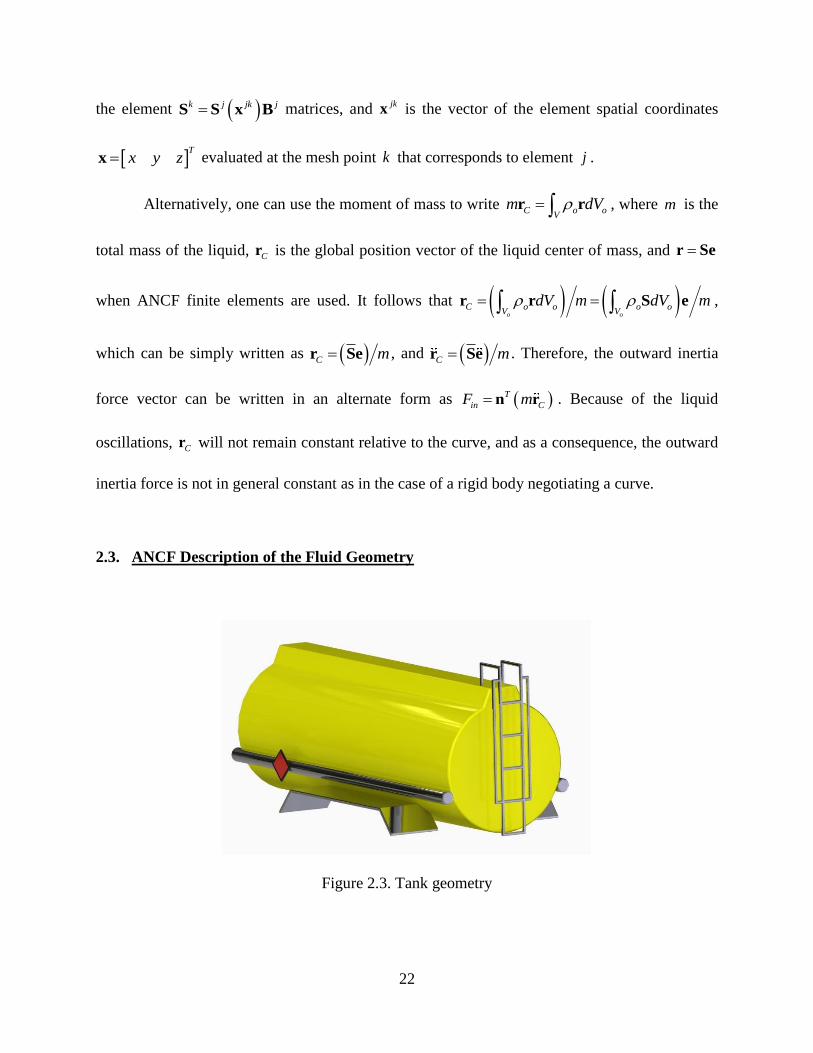
2.3. ANCF Description of the Fluid Geometry
Figure 2.3. Tank geometry

23
In this section, the development of the initially curved ANCF geometry of the fluid that assumes
the shape of a rigid cylindrical tank is discussed. The tank used in this chapter has a cylindrical
geometry as shown in Fig. 2.3, and therefore, it is required for the ANCF fluid mesh to have the
same the shape of the container it fills and at the same time represent different levels of the free
surface. The use of the ANCF absolute positions and gradients as nodal coordinates allows for
efficient shape manipulation and for obtaining the accurate complex geometry without the need
for using the CAD B-spline and NURBS representations that have rigid recurrence structure
(Shabana, 2015; Patel et al., 2016). As previously mentioned, in the ANCF description, the
assumed displacement field can be written as ( , ) ( ) ( )t t=r x S x e , where r is the global position
vector, [ ]Tx y z=x is the vector of the element spatial coordinates, t is time, S is the time-
independent element shape function matrix, and e is the vector of the element nodal coordinates
that include absolute position and gradient coordinates (Shabana, 2017A). The superscript j that
refers to the element number is omitted here for notational simplicity. The vector of element nodal
coordinates e can be written as o d= +e e e , where oe is the vector of nodal coordinates in the
reference configuration and de is the vector of nodal displacements. The assumed displacement
field can then be written as ( )( , ) ( ) ( ) ( )o dt t t= +r x S x e e . Using the general continuum mechanics
description ( )( , ) ,t t= +r X X u X , where X is the absolute position vector of an arbitrary point in
the reference configuration and u is the displacement vector, one can write o=X Se and d=u Se .
By choosing the elements in the vector oe appropriately, initially curved structures can be defined
in a straightforward manner using ANCF elements (Shabana, 2015).

24
Figure 2.4. Initially curved fluid geometry
The fully-parameterized ANCF solid element (Olshevskiy et al., 2013; Wei et al., 2015),
based on an incomplete polynomial representation, is used in this chapter to represent the fluid by
applying the proper fluid constitutive model which will be discussed in Section 2.4. In this case,
the arbitrary fluid material point on element j can be written as
8,1 ,2 ,3 ,4
1
j k k k k jk j j
k
S S S S=
= = r I I I I e S e , where I is the 3 3 identity matrix; detailed shape
function and nodal coordinate expressions can be found in Appendix C of this thesis. For example,
consider the element j which has the initially curved structure shown in Fig. 2.4. The matrix of
position vector gradients at node k can be written as ( ) ( ) ( ) ( ) jk jk jk jk
x y zo o o o
= xr r r r . For the
specific element geometry shown in Fig. 2.4, by adjusting the magnitude of the gradient vector
( )1j
yo
r without changing the gradient vector orientation, the position vector gradients at node 5 will
be ( ) ( ) ( ) ( )5 5 5 5 j j j j
x y zo o o o
= xr r r r , where is the stretch factor used to represent the stretch

25
of the edge; the value of can be obtained by taking the ratio between the arc lengths of curves
5-8 and 1-4. Following this procedure, the complex geometry of the fluid structure can be created,
as shown in Fig. 2.5. The mesh used in this chapter consists of 48 ANCF solid elements and the
mesh has a total number of degrees of freedom of 1260.
Figure 2.5. ANCF fluid mesh
2.4. ANCF Fluid Constitutive Model
A general ANCF fluid constitutive model that can account for the initially curved configuration is
developed in this section. The proposed fluid model ensures the continuity of the displacement
gradients at the nodal points and allows for imposing a higher degree of continuity across the
element interface by applying algebraic constraint equations that can be used to eliminate
dependent variables and reduce the model dimensionality at the prepossessing stage (Wei et al.,
2015). In order to describe the fluid-structure interaction, the penalty approach, described in
Section 2.5, is used to evaluate the contact and friction forces between the fluid and the rigid tank.
By using the non-modal ANCF approach, the fluid elastic forces can be formulated without
imposing restrictions on the amount of deformation and rotation within the elements. Figure 2.6

26
shows the three configurations of the fluid; the straight, curved reference, and current
configurations. As previously mentioned, the volume of the fluid in the curved reference
configuration oV is related to the volume in the straight configuration V using the relationship
o odV J dV= , where o oJ = J is the determinant of the matrix of position vector gradients
( )o o= = J X x Se x . Therefore, integration with respect to the reference domain can be
converted to integration with respect to the straight element domain. This allows for using the
original element dimensions to carry out the integrations associated with the initially curved
configuration.
Figure 2.6. Fluid configurations
The matrix ( )o o= J Se x is constant and can be evaluated at the integration points using
the ANCF element shape function and the vector of nodal coordinates in the reference
configuration (Shabana, 2015). The matrix of position vector gradients X Y Z= =J r X r r r ,
which is used to determine the Green-Lagrangian strain tensor ( ) 2T= −ε J J I , can be written as

27
( ) ( ) ( )1
1
x y z x y z e oo oo
−− = = = =
r r xJ r r r r r r J J
X x X, where
( )e = = J r x Se x . The relationship between the volume defined in the current configuration
v and the volume in the curved reference configuration oV can be written as odv JdV= where
J = J . It follows that 1
o e o o edv JdV J dV J dV−= = =J J .
The linear fluid constitutive equations can be defined using the Cauchy stress tensor and
can be assumed as ( ) tr 2 vol devp = − + + = +σ D I D σ σ where the temperature effect is
neglected and the fluid is assumed to be incompressible, σ is the symmetric Cauchy stress tensor,
p is related to the hydrostatic pressure, and are Lame’s material constants, I is a 3 3
identity matrix, tr refers to the trace of a matrix, and D is the rate of deformation tensor (Spencer,
1980; Shabana, 2017A). If the incompressibility condition is imposed using a penalty method, the
first two terms will vanish and the constitutive model reduces to 2dev dev=σ D . It is convenient to
use the second Piola-Kirchoff stress tensor since it is associated with the Green-Lagrangian strain
tensor defined in the reference configuration. One has 1 1 1 1
2 2T T
P dev devJ J− − − −= =σ J σ J J D J , where
1 1T− −=D J εJ , ( )T T 2= +ε J J J J and = J r X . For an arbitrary element j in the fluid body, the
virtual work of the fluid stress forces can be written as
1
2: :j j
o
j j j j j j j j
s dev P o
v V
W dv dV −
= − = − σ J J σ ε (2.1)
where ( )j j j j = ε ε e e . The virtual work of the fluid viscous forces can then be written as
( )1 1
2 : 2T
j jo o
j j j j j j j j j j j j
s P o r r o v
V V
W dV J dV − −
= − = − = σ ε C ε C : ε Q e (2.2)

28
where Tj j j
r =C J J is the right Cauchy-Green deformation tensor, and upon using the identity
1 1T Tj j j j j j
e o e oJ − −= = =J J J J J , the vector of generalized viscosity forces j
vQ associated with the
ANCF nodal coordinates can be written as
( ) ( )
( )
1 1 1 1
1 1
02 2
2
j jo
j
j jj j j j j j j j j j j j
v r r o r rj j
V V
jj j j j j
e r r j
V
J dV J dV
J dV
− − − −
− −
= − = −
= −
ε εQ C ε C : C ε C : J
e e
εC ε C :
e
(2.3)
In this case, the integration over the current configuration domain is converted to integration over
the straight configuration domain.
The incompressibility condition is imposed using the penalty method. Figure 2.6 shows
that the volume relation between the reference and current configuration is j j j
odv J dV= , therefore,
1j jJ = =J and 0jJ = still hold for the initially curved fluid. By assuming the penalty energy
function ( )2
1 2j j j
IC ICU k J= − and the dissipation function ( )2
2j j j
TD TDU c J= , where j
ICk and j
TDc
are the two penalty coefficients, the generalized penalty forces associated with the ANCF nodal
coordinates that result from imposing the two penalty conditions can be defined as
( )( )
( )
1
=
T
T
j j j j j j j
IC IC IC
j j j j j j j
TD TD TD
U k J J
U c J J
= = −
=
Q e e
Q e e (2.4)
where ( )trj j jJ J= D and j j j jJ J = e e . Knowing that
( ) ( ) ( )j j j j j j j j j j
X Y Z Y Z X Z X YJ = = = r r r r r r r r r , j jJ e can be written more explicitly, by
differentiating any of the three expressions for jJ with respect to
je , as
( ) ( ) ( )T T T
T Tj j
j j j j j j j j j
X Y Z Y Z X Z X Yj j
J J = = + +
S r r S r r S r r
e e (2.5)

29
By defining the generalized forces associated with the fluid element coordinates j
e , the
generalized forces associated with the fluid body coordinates e can be obtained using a standard
FE assembly procedure.
2.5. Fluid-Tank Interaction
The fluid should remain inside the tank regardless of the severity of the sloshing and these
boundary conditions of the mesh can be defined in multiple ways. One can impose constraints on
the boundary nodes, using either Lagrange multipliers or elimination of dependent variables.
Because this method is often more computationally expensive, in this thesis, the penalty method
is used to formulate the interaction between the fluid body and the rigid tank walls. The tank
deformation is not considered in this analysis because the main focus of this thesis is on studying
the sloshing. Figure 2.7a shows the contact geometry in the radial direction; the radius of the tank
is tr , superscript t refers to the tank,
fr is an arbitrary point on the fluid body, and
tR is the
position vector of the tank reference point defined in the global coordinate system. The position of
an arbitrary point of the fluid defined in the tank local coordinate system can be written as
( ) 1 2 3
T T Tft t ft t f t ft ft ftu u u = = − = u A u A r R , where
tA is the 3 3 transformation matrix
which defines the tank orientation, and the bar notation means the vector or matrix is defined in
the body local coordinate system. The inequality ( ) ( ) ( )2 2 2
2 3
ft ft tu u r+ implies that the fluid point
is inside the tank and there is no need for applying a penalty force. On the other hand, the equation
( ) ( ) ( )2 2 2
2 3
ft ft tu u r+ implies that penalty forces must be applied in order to prevent the fluid from
penetrating the tank walls. In this case, the penetration can be evaluated as
( ) ( )2 2
2 3
ft ft tu u r = + − . The unit normal n at the fluid/tank contact point can be defined as
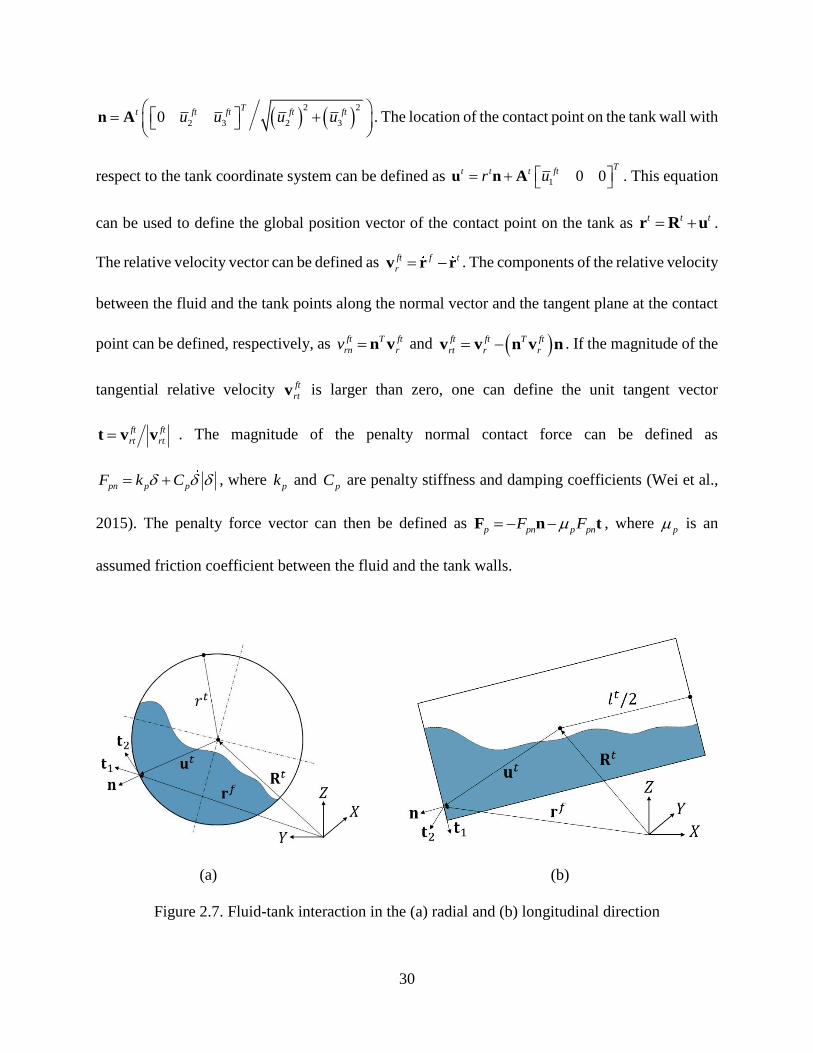
30
( ) ( )2 2
2 3 2 30T
t ft ft ft ftu u u u = +
n A . The location of the contact point on the tank wall with
respect to the tank coordinate system can be defined as 1 0 0T
t t t ftr u = + u n A . This equation
can be used to define the global position vector of the contact point on the tank as t t t= +r R u .
The relative velocity vector can be defined as ft f t
r = −v r r . The components of the relative velocity
between the fluid and the tank points along the normal vector and the tangent plane at the contact
point can be defined, respectively, as ft T ft
rn rv =n v and ( )ft ft T ft
rt r r= −v v n v n . If the magnitude of the
tangential relative velocity ft
rtv is larger than zero, one can define the unit tangent vector
ft ft
rt rt=t v v . The magnitude of the penalty normal contact force can be defined as
pn p pF k C = + , where pk and
pC are penalty stiffness and damping coefficients (Wei et al.,
2015). The penalty force vector can then be defined as p pn p pnF F= − −F n t , where
p is an
assumed friction coefficient between the fluid and the tank walls.
(a) (b)
Figure 2.7. Fluid-tank interaction in the (a) radial and (b) longitudinal direction

31
Knowing the ANCF element j on which the fluid/tank contact point lies, one can develop
an expression for the generalized penalty contact forces associated with the fluid element nodal
coordinates. The virtual work of the penalty force acting on the fluid and tank can be written as
T f T t
p p pW = −F r F r , which can be written as ( )T j j T t t t t
p p pW = − −F S e F R u G θ (Shabana,
2013), where j
S is the element shape function matrix evaluated at the contact point, t
u is the skew
symmetric matrix associated with the vector t
u , and t
G is the matrix that relates the absolute
angular velocity vector t
ω of the tank to the time derivatives of the tank orientation parameters
tθ , that is,
t t t=ω G θ . It follows that the generalized reaction forces exerted on the element j of
the ANCF fluid body can be written as Tj j
ep p=Q S F , while the generalized penalty forces exerted
on the tank and associated with the tank reference coordinates t
R and tθ are given, respectively,
as
,Tt i t t
R p p= − = −F F F G u F (2.6)
A similar procedure can be used to evaluate the interaction forces between the fluid and the rigid
tank in the longitudinal direction. This contact geometry is shown in Fig. 2.7b.
2.6. Vehicle Model Components
The MBS model used in this chapter consists of 21 bodies which have 147 absolute coordinates
because Euler parameters are used to describe the body orientations. These bodies are subjected to
115 constraint equations, leading to a model with 32 degrees of freedom. The 10 tires are modeled
using Pacejka’s brush tire model, which is discussed in Section 2.6.1 (Pacejka, 2006). The four-
bar Ackermann steer axle, which allows the truck to turn, is described in Section 2.6.2. Other
bodies include two rear axles, the cab, the tank, the frame rails, and a ground body. Inertial
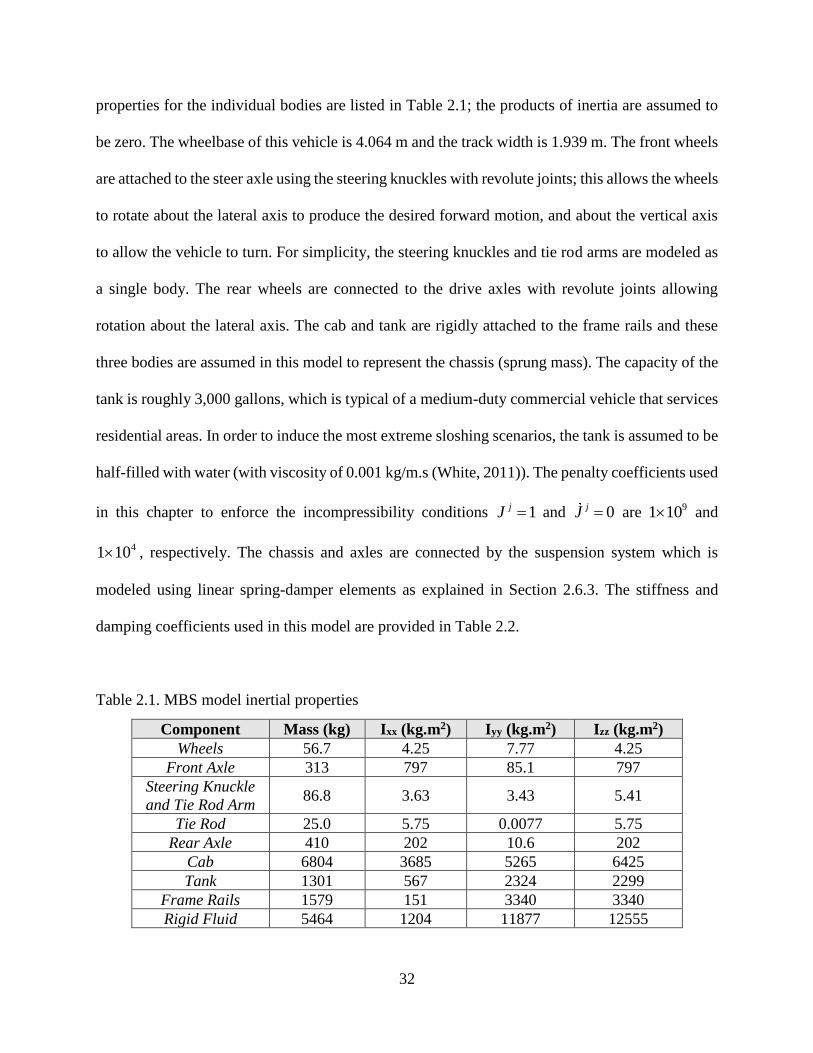
32
properties for the individual bodies are listed in Table 2.1; the products of inertia are assumed to
be zero. The wheelbase of this vehicle is 4.064 m and the track width is 1.939 m. The front wheels
are attached to the steer axle using the steering knuckles with revolute joints; this allows the wheels
to rotate about the lateral axis to produce the desired forward motion, and about the vertical axis
to allow the vehicle to turn. For simplicity, the steering knuckles and tie rod arms are modeled as
a single body. The rear wheels are connected to the drive axles with revolute joints allowing
rotation about the lateral axis. The cab and tank are rigidly attached to the frame rails and these
three bodies are assumed in this model to represent the chassis (sprung mass). The capacity of the
tank is roughly 3,000 gallons, which is typical of a medium-duty commercial vehicle that services
residential areas. In order to induce the most extreme sloshing scenarios, the tank is assumed to be
half-filled with water (with viscosity of 0.001 kg/m.s (White, 2011)). The penalty coefficients used
in this chapter to enforce the incompressibility conditions 1jJ = and 0jJ = are 91 10 and
41 10 , respectively. The chassis and axles are connected by the suspension system which is
modeled using linear spring-damper elements as explained in Section 2.6.3. The stiffness and
damping coefficients used in this model are provided in Table 2.2.
Table 2.1. MBS model inertial properties
Component Mass (kg) Ixx (kg.m2) Iyy (kg.m2) Izz (kg.m2)
Wheels 56.7 4.25 7.77 4.25
Front Axle 313 797 85.1 797
Steering Knuckle
and Tie Rod Arm 86.8 3.63 3.43 5.41
Tie Rod 25.0 5.75 0.0077 5.75
Rear Axle 410 202 10.6 202
Cab 6804 3685 5265 6425
Tank 1301 567 2324 2299
Frame Rails 1579 151 3340 3340
Rigid Fluid 5464 1204 11877 12555

33
2.6.1. Brush Tire Model
In this thesis, the forces exerted on the tires by the ground are calculated using the brush tire model
(Pacejka, 2006). Four coordinate systems which define the orientations of the tire body i and the
ground body j are introduced. The ground coordinate system which describes the orientation of
the ground body is given by the matrix j j j j = A i j k , where the columns j
i , jj , and
jk
are unit vectors along the ground coordinate axes j j j
X Y Z . In this chapter, j
A is assumed to be
the identity matrix except in the case of uneven terrains, such as a hill, bumpy road, or inclined
ramp. The three other coordinate systems are used in the tire formulation and are depicted in Fig.
2.8. The tire coordinate system defined by the matrix i i i i = A i j k is rigidly attached to the
center of the tire and rotates with the tire. The matrix i i i i
o o o o = A i j k describes the
intermediate tire coordinate system (ITCS) which is also rigidly attached to the center of the tire,
but does not share the pitch rotation with the tire. The axes of i
oA are defined as
( )i i j i i j i
o =
A j k j j k j . Finally, the contact point coordinate system located at the
contact point between the ground and the tire is defined by the matrix
i i i i i i i j
c c c c o c c = = − A i j k i k i k . Using the ITCS transformation matrix i
oA , the contact
point between the tire and the ground can be defined as i i i i
c o oc= +r R A u , where i
R is the global
position of the ITCS origin and i
ocu is the position of the contact point with respect to the ITCS
origin. The velocity vector of the contact point can then be obtained by differentiating the position
vector with respect to time, and is defined as i i i i
c oc= + r R ω u , where i
R is the velocity of the
ITCS origin, i
ω is the absolute angular velocity vector of the tire defined in the global coordinate
system, and i i i
oc o oc=u A u .

34
Figure 2.8. Brush Tire model coordinate systems
The brush tire model accounts for the normal, lateral, longitudinal, and rotational friction
forces, as well as an aligning torque, also referred to as the spin moment in rail vehicle dynamics.
In this thesis, it is assumed that the material properties are the same in the lateral and longitudinal
directions, which is a simplifying assumption often made in the literature (Pacejka, 2006; Patel et
al., 2016; Pelc, 2007; Bolarinwa et al., 2012; Bruzelius et al., 2013). The normal force in the
contact point coordinate system is calculated simply as 1.5 | |z z z zF K C = − − where K is the
radial stiffness coefficient of the tire, z is the vertical penetration of the tire with the ground, C
is the radial damping coefficient, and z is the rate of change of the penetration. In order to
determine the lateral and longitudinal friction forces, the slip angle and slip ratio vector ξ are
needed. First, the slip velocity sv is defined as 0 0TT i i
s sx sx c rc c rcv v = = v i v j v ,
where rcv is the velocity of the tire with respect to the ground at the contact point. The slip ratio

35
vector ξ is 0 0T T
x y sx r sy rv v v v = = − − ξ , where rv is the tire forward velocity.
The slip angle is determined as ( )1tan y −= . The model parameter is defined as
22 / 3p zc a F = where pc is the tread element stiffness per unit length, a is half the contact
patch length, is the friction coefficient, and zF is the magnitude of the normal force. The
coefficients pc and are specified for both the lateral and longitudinal directions, so both x
and y can assume different values. In this thesis, it is assumed that
, ,p x p yc c= and x y = , so
x y = . The slip angle where the pure sliding starts, sl , is defined as ( )1tan 1sl −= .
The lateral and longitudinal friction forces on tire body i in the contact point coordinate
system are determined by ( ) ( )3sgn 1i
j sj j z jF v F = − − if | | sl and ( )sgni
j sj j zF v F= − if
| | sl for ,j x y= where 1j j j = − is a simplifying model parameter. The aligning torque
i
zM is also calculated in the contact point coordinate system depending on the slip angle , as
( ) ( ) 3sgn 1i
z y z y yM aF = − − if | | sl or 0i
zM = if | | sl in the case of pure sliding. To
determine the moment due to the rotational friction force ( )i
y rM in the intermediate tire coordinate
system, a sinusoidal function is used to smooth the forces near 0y = . This moment is defined as
( ) ( )sgni
y y r zrM F = − if | |y t and ( ) ( )sgn( ) sin | | 2
i
y y r z y trM F = − when | |y t ,
where r is the rotational friction coefficient, and t is assumed to be 101.0 10− . The forces and
moments obtained in this section for the tire can be defined in the appropriate coordinate system
for the inclusion in the Newton-Euler equations that govern the motion of the tire which is treated
in the brush model as a rigid body.

36
2.6.2. Ackermann Steering Mechanism
Figure 2.9. Ackermann steering mechanism
In order for a vehicle to be able to negotiate a turn with minimal tire scrub, the Ackerman steering
mechanism is often used. The Ackermann steering system is a four-bar mechanism which allows
the wheels to be oriented at different angles with respect to the forward direction. The four-bar
mechanism consists of the front axle as the ground link, two tie rod arms, and a tie rod, as shown
in Fig. 2.9. The tie rod is connected to the tie rod arms with spherical joints to avoid over-
constraining the mechanism. By specifying the geometry of the Ackerman mechanism, each of the
front wheel forward velocity vectors remains tangent to a circular arc whose origin is located at
the instantaneous center of rotation of a line element connecting the centers of the two wheels,
thus reducing tire scrub. The linkage geometry can be defined by two equations, cosh r = and
2 sins t r = − , where h is the distance between the axle and the tie rod, r is the length of the tie
rod arm, is the angle between the tie rod arm and the normal to the axle, s is the length of the
tie rod, and t is the length of the axle, as shown in Fig. 2.10. Because the length of the axle and
the wheelbase are known for the vehicle model used in this chapter to be 1.939 m and 4.064 m,

37
respectively, can be calculated as 13.42o. In the optimization study by De-Juan et al. (2012), it
was found that for an axle length of 1.5 m, the optimum tie rod length and tie rod arm length are,
respectively, 1.27 m and 0.3 m. To determine the remaining parameters of the steering mechanism,
it was assumed that the steering mechanism dimensions are proportional to the dimensions of the
optimal mechanism geometry obtained in the study by De-Juan et al. (2012). Using this assumption,
the geometry parameters obtained were r = 0.3878 m, s = 1.7590 m, and h = 0.3772 m.
Figure 2.10. Steering mechanism geometry
2.6.3. Suspension System Design
The suspension system of the truck is modeled using linear spring-damper elements, the
parameters of which are listed in Table 2.2. The spring-dampers are oriented to provide restoring
forces in the longitudinal, lateral, and vertical directions – the vertical springs are used to support
the weight of the chassis, cab, tank, and fluid, while the longitudinal and lateral springs are used
to prevent relative motion in the longitudinal and lateral directions, respectively. The spring-
dampers are located at each end of the three axles, resulting in 18 elements total. The vertical
springs on the rear axles are initially compressed to aid in supporting the weight of the tank and

38
fluid and to minimize oscillations at the beginning of the simulation when the vehicle reaches
equilibrium.
Table 2.2. Suspension parameters
X Direction Y Direction Z Direction
Spring
(N/m)
Damper
(N.s/m)
Spring
(N/m)
Damper
(N.s/m)
Spring
(N/m)
Damper
(N.s/m) 91.25 10 41 10 85 10 41 10 67.5 10 55 10
2.7. Specified Motion Trajectories
In numerical simulations, two methods can be used to produce the MBS motion; the first is to
apply forces on the system components, while the second is to specify motion trajectories using
algebraic constraint equations. The latter approach of using constraint equations is more
appropriate when it is required to precisely follow certain trajectories and correctly capture their
geometry, as is the case in this chapter. In order for the tanker truck model to follow different
specified paths necessary to create the motion scenarios to be investigated in this chapter, trajectory
coordinate constraints must be imposed. Three coordinate systems are used to define the type of
the trajectory coordinate constraint used in this thesis: the global coordinate system XYZ , the
trajectory coordinate system ti ti tiX Y Z , and the body coordinate system
ir ir irX Y Z , as shown in
Fig. 2.11 (Shabana et al., 2008). Six trajectory coordinates i
p are used to specify the motion of a
body, where T
i i ir ir ir ir irs y z = p , is is the arc length along the user-specified
trajectory, iry and
irz are the lateral and vertical displacements of the body with respect to the
specified trajectory, and ir ,
ir , and ir are the three Euler angles describing the relative
rotations of the body coordinate system with respect to the trajectory coordinate system. Because

39
a curve can be completely defined using one parameter, Frenet frame geometry is employed to
write the matrix ti
A that defines the orientation of the trajectory coordinate system in terms of
three Euler angles ti , ti , and ti which can be expressed in terms of the arc length parameter
is as ( )ti ti is = , ( )ti ti is = , and ( )ti ti is = (Shabana et al., 2008). The transformation
matrix ir
A that defines the orientation of the body coordinate system with respect to the trajectory
coordinate system is developed using the three time-dependent Euler angles ( )ir t , ( )ir t , and
( )ir t . Using this description, the global position vector of an arbitrary point on the body can be
written as i i i i
p p= +r R A u , where i
R is the global position of the origin of the body coordinate
system, i ti ir=A A A is the transformation matrix which defines the orientation of the body
coordinate system in the global coordinate system, and i
ppu is the position vector of the arbitrary
point, defined in the body coordinate system.
Figure 2.11. Trajectory constraint coordinate systems

40
While trajectory coordinate constraints can be applied to the translation and/or orientation
of a body, only translational coordinate constraints are needed in this thesis to specify the vehicle
forward motion during straight line motion, rapid lane change, and curve negotiation. A
translational trajectory coordinate constraint on body i can be written as R, ( ) 0i
k kC p f t= − = for
1,2,3k = , where kC is the constraint function corresponding to the trajectory coordinate R,
i
kp ,
R,
i
kp is the thk component of
Ti i ir ir
R s y z = p , and ( )f t is the time-varying function
defining the values of the trajectory coordinate ,
i
R kp . For example, to constrain the vehicle to move
along a specified path with a constant forward velocity sV , the constraint applied to the body
coordinate system of the front axle can be written as 0i i
o sC s s V t= − − = , where i
os is the initial
arc length coordinate. Because in this thesis, the equations of motion are developed using the
absolute Cartesian coordinate formulation, it is necessary to define the trajectory coordinates in
terms of the absolute Cartesian coordinates using the relationship
( ), ,i ir ir i ti ti irs y z = − − =g R R A u 0 , where ir
R is the global position of the body coordinate
system with respect to the trajectory coordinate system and ir
u is the position vector of the center
of mass of the body in the trajectory coordinate system. For a given set of absolute Cartesian
coordinates, this set of nonlinear equations can be solved iteratively to determine the arc length
parameter is as well as the coordinates
iry and irz . The constraint Jacobian matrix associated
with the absolute Cartesian coordinates can also be systematically developed and used to enforce
the constraints at the position, velocity, and acceleration levels. The driving constraint forces that
produce the desired motion can be determined using Lagrange multipliers and the trajectory
coordinate constraint Jacobian matrix (Shabana et al., 2008).

41
2.8. Equations of Motion
The vectors and matrices defined in the previous sections enter into the general formulation of the
equations of motion for the MBS vehicle model, which may include rigid and flexible bodies. The
equations of motion can be written as (Shabana et al., 2008):
r
r
T
r rr
Tee
T
d
=
q
e
s
q e s
M 0 0 C Qq
Qe0 M 0 C
0s0 0 0 C
QλC C C 0
(2.7)
where rM and eM are the mass matrices associated with the rigid and flexible ANCF body
coordinates, respectively, rqC , eC , and sC are the constraint Jacobian matrices associated with
the rigid, elastic, and non-generalized trajectory coordinates, respectively, rq , e , and s are the
accelerations of the rigid reference, elastic, and non-generalized trajectory coordinates,
respectively, λ is the vector of Lagrange multipliers associated with the constraints, rQ and eQ
are the vectors of generalized forces associated with the rigid and elastic coordinates, respectively,
and dQ is a vector resulting from the second time derivative of the vector of constraint equations.
The equations of motion are solved numerically using the Adams-Bashforth integration technique,
and a solution algorithm that ensures that the constraint equations are satisfied at the position,
velocity, and acceleration levels. Because the equations of motion are second order differential
equations, two sets of initial conditions (coordinates and velocities) are required to obtain a unique
solution. The initial coordinates and velocities of the rigid bodies, 0r
q and 0r
q , the initial
coordinates and velocities of the nodes of the flexible ANCF bodies, 0e and 0e , and the initial
non-generalized coordinates and velocities 0s and 0s are user-specified and known at the
beginning of the simulation. The initial velocities of all bodies and nodes vary depending on the

42
maneuver being considered in the numerical simulation. These maneuver scenarios are presented
in Table 2.3.
Table 2.3. Initial velocities
Maneuver Braking Lane Change Curve Negotiation
Initial Velocity
(mph) 55 55 25
2.9. Numerical Results
Figure 2.12. Commercial medium-duty tanker truck model
The dynamic behavior of the tanker truck model, created in the MBS dynamics software
SIGMA/SAMS and shown in Fig. 2.12 was examined using three different motion scenarios, each
of which produces different fluid motion. In the first scenario, the truck decelerates under straight-
line motion, such that the fluid primarily exerts longitudinal forces on the tank. In the second
scenario, the truck performs a lane change, which causes the fluid to exert alternating lateral forces
on either side of the tank. In contrast, in the third scenario the truck is assumed to negotiate a wide

43
curve, such that the lateral motion of the fluid is continuous and exerted on one side of the tank
only. Steady state is achieved before the simulation results are reported in order to eliminate the
transient effects. Another model in which the fluid is represented by a rigid body with equivalent
inertial properties was also created; the rigid fluid body is rigidly attached to the tank so that the
sloshing motion is prevented but the fluid inertia is correctly accounted for. This model was also
examined using the same three scenarios so that the effect of the fluid sloshing on vehicle dynamics
can be isolated and evaluated.
2.9.1. Straight Line Deceleration Scenario
Figure 2.13. Velocity during braking
For this scenario, the truck begins at a highway speed of 55 mph and brakes to 20 mph as seen in
the velocity - position plot in Fig. 2.13. This scenario could occur if braking is suddenly applied
in an attempt to avoid a rear-end collision. As seen in Fig. 2.14, the sloshing phenomenon is clearly
evident as the fluid moves in the longitudinal direction towards the front end of the tank as a result

44
of the sudden braking. It is important to note that the section on the top of the tank is an exterior
section that the fluid cannot enter (refer to Fig. 2.3); therefore, the fluid fills the front portion of
the tank during braking.
Figure 2.14. Fluid sloshing due to braking
Figure 2.15. Normal force on a front tire and a rear tire during braking
( Rigid model front tire, ANCF model front tire,
Rigid model rear tire, ANCF model rear tire)

45
Figure 2.16. Position of fluid center of mass relative to tank during braking
( Longitudinal direction, Lateral direction, Vertical direction)
The normal forces increase on the front tires and decrease on the rear tires, as evident in
Fig. 2.15, because the center of mass of the fluid moves towards the front of the tank, as seen in
the plot of the fluid center of mass presented in Fig. 2.16. A second peak occurs in the contact
forces on the front tires near 7s due to the rebounding motion of the fluid after it impacts the rear
of the tank and again sloshes longitudinally towards the front of the tank. Although the normal
forces also increase on the front tires and decrease on the rear tires in the equivalent rigid body
model due to the shift in inertia of the chassis on the suspension system, also seen in Fig. 2.15, the
magnitudes are much less significant because the center of mass of the rigid fluid body remains
constant with respect to the tank and the relative displacement of the chassis on the suspension
system is small compared to the longitudinal displacement of the flexible fluid. The fluid free
surface of the ANCF model returns to a flat shape once the truck reaches the lower speed, as seen

46
in Fig. 2.17, and the normal forces return to approximately equilibrium in both models, as evident
by the results presented in Fig. 2.15.
Figure 2.17. Flat free surface at steady state after braking
2.9.2. Lane Change Scenario
Figure 2.18. Lane change trajectory
47
In the second motion scenario, the truck performs a lane change over a standard-width US highway
lane of 3.7m, as seen in the plot of lateral - longitudinal position in Fig. 2.18. The lane change is
completed in a relatively short time of 4s so that the fluid sloshing readily occurs, as seen in the
series of images in Fig. 2.19 depicting the change in the free surface of the fluid mesh. The shift
in the center of mass of the flexible fluid mesh as the truck negotiates the turns of the lane change
causes the normal forces exerted on the tires on the outer edge of the curve to be greater than those
exerted on the inner tires, as seen in Fig. 2.20. For the first half of the lane change, the left tire (Fig.
2.20a) is the inner tire, and for the second half of the lane change, the right tire (Fig. 2.20b) is the
inner tire. This effect is also evident in the rigid body model due to the outward inertia forces,
however the peak forces exerted are greater for the ANCF model than for the rigid body model
due to the sloshing behavior, which is evident in the plot of the fluid center of mass presented in
Fig. 2.21. Furthermore, it can be seen that the peaks in the normal forces on the outer tires of the
rigid body model are the same after both the first and second halves of the lane change – 8 kN on
the inner tire and 20.5 kN on the outer tire in both cases. However, this is not the case for the
ANCF model tires – the changes in the normal forces from equilibrium are greater after the second
half of the lane change (5.5 kN and 22.5 kN) as compared to the first (6.5 kN and 21 kN). This is
because the forces of the tank walls on the fluid during the second half of the lane change act in
the same direction as the motion of the rebounding fluid, causing the lateral shift of the fluid to be
larger than would have occurred due to free vibration only. After the lane change is completed, the
normal forces on the tires of the ANCF model oscillate about a nominal value due to the lateral
sloshing of the fluid, whereas the normal forces remain at steady-state after the rigid fluid model
negotiates the lane change because the lateral position of the fluid is fixed with respect to the tank.

48
Figure 2.19. Lateral sloshing due to lane change maneuver
Figure 2.20. Normal force on (a) a left-hand tire and (b) a right-hand tire during a lane change
( Rigid model, ANCF model)

49
Figure 2.21. Position of fluid center of mass relative to tank during lane change
( Longitudinal direction, Lateral direction, Vertical direction)
Figure 2.22. Lateral friction force on (a) a left-hand tire and (b) a right-hand tire during a lane
change
( Rigid model, ANCF model)

50
These effects are also apparent in the lateral friction force results presented in Fig. 2.22.
The peak lateral friction force on the inner tire is comparable between the ANCF model and the
rigid body model because although the normal force is less for the ANCF model tire due to the
outward shift of the fluid, the lateral velocity of the tire with respect to the ground is greater for
the ANCF model tire, which negates the effect of the decreased normal force. This is clear from
the results presented in Fig. 2.23, where the lateral slip velocity of a left tire is greater for the
ANCF model during the lane change.
Figure 2.23. Lateral slip velocity on a left-hand tire during a lane change
( Rigid model, ANCF model)
2.9.3. Curve Scenario
For the third scenario, the truck negotiates a wide curve as seen in Fig. 2.24, similar to an onramp
or exit ramp of a highway, except that the bank angle is assumed zero for simplicity. While driving
along a road of constant curvature and in the case of zero bank angle, the outward centrifugal force
on a rigid vehicle due to the curve of the road is counteracted by the lateral friction force exerted

51
on the tires; that is, 2
smV r mg= where m is the mass of the vehicle, sV is the forward velocity,
r is the radius of curvature of the road, is the coefficient of friction between the tires and the
road, and g is the gravitational constant.
Figure 2.24. Curve trajectory
As previously discussed in this paper, the maximum speed at which the vehicle can traverse
a curve without sliding can then be calculated as sV gr= . For example, for a radius of curvature
of 115 ft and a coefficient of friction of 0.7, the maximum calculated speed is 33.9 mph. However,
due to the high center of gravity of the truck and increased chance of rollover, in practice vehicles
cannot traverse a curve at the theoretical maximum speed. According to the National Highway
Traffic Safety Administration (NHTSA), the maximum speed at which an average fully-loaded
tractor-trailer can negotiate a curve of 150 ft is 30mph; at greater speeds, the chance of rollover is
greatly increased (U.S. Department of Transportation, NHTSA, 2015). Therefore, for this analysis,
the constant forward speed is chosen to be 25 mph and the radius of curvature of the track is set to

52
150 ft. As previously mentioned, the road is assumed to be flat with no super-elevation; this
assumption is consistent with methods used in the literature (Pape et al., 2016).
Figure 2.25. Normal force on an outer tire and an inner tire during curve negotiation
( Rigid model outer tire, ANCF model outer tire,
Rigid model inner tire, ANCF model inner tire)
Figure 2.26. Lateral friction force on (a) an outer tire and (b) an inner tire during curve
negotiation
( Rigid model, ANCF model)

53
The normal and lateral forces exerted on the tires of the rigid body model are larger on the
outer tires and smaller on the inner tires, as seen in Figs. 2.25 and 2.26, respectively. This is due
to the roll moment that is exerted from the centrifugal force on the vehicle. Because the radius of
curvature is constant and the center of mass of the fluid in the rigid body model is not able to move,
the centrifugal force is constant once the truck enters the curve, and thus the normal and lateral
forces are constant as well. The contact forces on the tires of the ANCF model, however, overshoot
the constant value exerted on the rigid body model tires, and oscillate due to the sloshing motion
and the change in the center of mass of the fluid, as seen in Figs. 2.25 and 2.26. Furthermore, while
the centrifugal force on the rigid fluid is 2
smV r as discussed in Section 2.2, it has been
demonstrated that this is not the case for flexible bodies (Shi et al., 2017). This is evident in Fig.
2.27, where the outward inertia force on the flexible fluid mesh oscillates with a maximum
amplitude that exceeds the nominal rigid body model value by nearly 16%. This oscillation is due
to the changing location of the center of mass of the fluid – while it is constant relative to the
vehicle for the rigid body model, the sloshing phenomenon occurring in the flexible model results
in oscillation of the center of mass, and thus the effective radius of curvature changes as the vehicle
negotiates the curve. The sloshing amplitudes and thus the inertia and contact forces decrease with
time for the ANCF model due to the fluid viscosity and the friction forces between the fluid and
tank walls. In order to better understand the results presented in Fig. 2.27, Fig. 2.28 shows the
position of the center of mass of the liquid with respect to the tank. This figure shows that because
of the liquid oscillations, the simple equation 2
smV r used to calculate the centrifugal force in
rigid body dynamics is no longer applicable in the case of liquid sloshing. Figure 2.29 shows the
components of the normalized velocity of the liquid center of mass obtained by dividing by the

54
vehicle forward velocity. Figure 2.29a shows the dimensionless velocity component tangent to the
curve, while Fig. 2.29b shows the other two components.
Figure 2.27. Outward inertia force on fluid during curve negotiation
( Rigid model, ANCF model)
Figure 2.28. Position of fluid center of mass relative to tank during curve negotiation
( Longitudinal direction, Lateral direction, Vertical direction)

55
Figure 2.29. Normalized velocity of the fluid center of mass in the (a) longitudinal and (b) lateral
and vertical directions
( Longitudinal direction, Lateral direction, Vertical direction)
The magnitudes of the contact forces are not identical to those predicted by the analytical
model in Section 2.1 because only two wheels were included in that analysis, and the weight of
the tank and fluid is actually distributed over 10 wheels. However, the orders of magnitude of the
contact forces are the same and the relative changes in the forces were well predicted, and thus the
analytical model verifies the simulation results.
2.10. Concluding Remarks
A total Lagrangian ANCF fluid formulation that can be systematically integrated with fully
nonlinear MBS vehicle algorithms is proposed in this chapter. The new approach can capture the
fluid distributed inertia and viscosity, can accurately predict the change in inertia due to the change
in shape of the fluid, and can visualize the change in the fluid free surface, unlike other discrete
inertia models which do not capture these significant details. The outward forces on the fluid
56
during curve negotiation are derived and it is shown that these forces do not take the same simple
form as the case of a rigid body negotiating a curve. As discussed in the paper, accurate modeling
of the fluid geometry using ANCF elements can be achieved without the need for using
computational geometry methods such as B-spline and NURBS representations which have a rigid
recurrence structure unsuitable for MBS analysis. By using the approach proposed in this chapter,
one geometry/analysis mesh is used from the outset. The fluid constitutive law and the fluid/tank
interaction forces are developed. The penalty method is used to ensure that the fluid remains within
the boundaries defined by the tank geometry. Both normal and tangential penalty contact forces
are considered in this chapter. The MBS vehicle model components are described and the
dynamics of the vehicle is examined using three contrasting motion scenarios in order to study the
effect of sloshing on vehicle dynamics. The braking scenario examines the case of longitudinal
sloshing of the fluid, a rapid lane change produces alternating lateral fluid forces on the tank, and
curve negotiation sheds light on the case of steady-state outward forces due to the centrifugal effect.
The results presented in this chapter demonstrate that depending on the scenario, the
sloshing phenomenon can increase the contact forces on some wheels while decreasing contact
forces on other wheels, and this can lead to vehicle instability. In the case of brake applications,
the fluid in the partially-filled tank surges forward, causing uneven wheel loading; in cases of
severe braking, wheel lift may occur on the rear wheels of the vehicle. This can lead to difficulty
controlling the vehicle and increased stopping distances due to lessened road contact, and the
decrease in stability may result in jack-knifing for tractor-trailer vehicles. When entering a curve
or performing a lane change, the outward centrifugal forces cause lateral displacement of the fluid,
which also causes uneven wheel loading. In extreme cases of high speed or small radius of
curvature, these changes could be significant enough to induce wheel lift on the inner wheels and

57
increase the possibility of rollover compared to an equivalent truck carrying rigid materials.
Furthermore, in cases where tire friction forces are decreased, such as on wet or icy roads, the
possibility for vehicle instability increases even further and drivers must exercise extra caution.
Future analysis can result in defining general rules for speed reduction of a tanker truck entering a
curve in order to maximize vehicle stability and driver safety, proposing modifications to the tank
geometry to reduce sloshing amplitudes and forces, studying the effect of viscosity and
incompressibility on the fluid dynamic behavior, and comparison with conventional finite
elements as well as the smoothed particle hydrodynamics (SPH) method (Wasfy et al., 2014).

58
CHAPTER 3
FLUID MODELING WITH RAILROAD VEHICLE APPLICATIONS
A new continuum-based liquid sloshing approach that accounts for the effect of complex fluid and
tank-car geometry on railroad vehicle dynamics is developed in this chapter (published as Shi et
al., 2017). A unified geometry/analysis mesh is used from the outset to examine the effect of liquid
sloshing on railroad vehicle dynamics during curve negotiation and during the application of
electronically controlled pneumatic (ECP) brakes that produce braking forces uniformly and
simultaneously across all cars. Using a non-modal approach, the geometry of the tank-car and fluid
is accurately defined, a continuum-based fluid constitutive model is employed, and a fluid-tank
contact algorithm is developed. The liquid sloshing model is integrated with a three-dimensional
multibody system (MBS) railroad vehicle algorithm which accounts for the nonlinear wheel/rail
contact. The three-dimensional wheel/rail contact force formulation used in this study accounts for
the longitudinal, lateral, and spin creep forces that influence the vehicle stability. In order to
examine the effect of the liquid sloshing on the railroad vehicle dynamics during curve negotiation,
a general and precise definition of the outward inertia force is defined, and in order to correctly
capture the fluid and tank-car geometry, the absolute nodal coordinate formulation (ANCF) is
used. The balance speed and centrifugal effects in the case of tank-car partially filled with liquid
are studied and compared with the equivalent rigid body model in curve negotiation and braking
scenarios. In particular, the results obtained in the case of the ECP brake application of two freight
car model are compared with the results obtained when using conventional braking. The traction
analysis shows that liquid sloshing has a significant effect on the load distribution between the

59
front and rear trucks. A larger coupler force develops when using conventional braking compared
with ECP braking, and the liquid sloshing contributes to amplifying the coupler force in the ECP
braking case compared to the equivalent rigid body model which does not capture the fluid
nonlinear inertia effects. Furthermore, the results obtained in this chapter show that liquid sloshing
can exacerbate the unbalance effects when the rail vehicle negotiates a curve at a velocity higher
than the balance speed.
3.1. Basic Inertia Force Definitions
A rail vehicle can safely negotiate a curve if the outward inertia force does not exceed the sum of
the lateral gravity force component and the inward friction force. However, as mentioned
previously, the centrifugal force of a flexible body does not take the simple form of 2mV R , where
m is the mass of the vehicle, V is the forward velocity, and R is the radius of curvature of the
curve (Shi et al., 2017). As presented in Chapter 2, a straightforward method to determine the
outward inertia force in the case of flexible body dynamics is to use the projection of the inertia
force vector on the outward normal to the curve, which has the form i
i i i
VdV r n in the case of
a flexible body i , where i and
iV are, respectively, the mass density and volume of the flexible
body, i
r is the acceleration vector, and n is the outward unit normal to the curve. This inertia
force expression is general and includes the effect of other deformation-dependent forces such as
gyroscopic moments and Coriolis forces.

60
3.1.1. FFR Inertia Forces
The form of the inertia forces depends on the method used to formulate the kinematic and dynamic
equations. When ANCF elements are used, the inertia forces take a simple form and the mass
matrix becomes constant. While ANCF elements will be used in this chapter, another widely used
formulation, the floating frame of reference (FFR), is used in this section to shed light on the form
of the inertia forces in the case of curve negotiation and to show that the rigid body assumption
leads to the definition of the centrifugal forces used in rigid body dynamics. To this end, a simple
planar example is used in this section (Shi et al., 2017).
Unlike the ANCF description, in the FFR formulation, a flexible body coordinate system
is introduced and the motion of a planar body i in the system is defined using two coupled sets of
coordinates, the reference coordinates T T
i i i
r =
q R and the elastic coordinates i
fq , where i
R
describes the body reference translation, i defines the reference orientation, and i
fq defines the
body deformation with respect to its reference. In the FFR formulation, there is no separation
between the rigid body motion and the elastic deformation, and therefore, the FFR description does
not imply any simplifying assumptions. The generalized coordinates for a planar deformable body
i can then be written as T T T
i i i i
f =
q R q . Using these generalized coordinates, the global
position vector of an arbitrary point on the deformable body can be written as
( )i i i i i i i i i
o f= + = + +r R A u R A u S q (3.1)
where iu is the local position vector defined in the body coordinate system, and
iA is the
transformation matrix that defines the body orientation and is expressed in terms of the angle i .
The local position vector iu can be written as i i
o f+u u , in which i
ou is local position vector of the

61
arbitrary point in the undeformed state and i
fu is the deformation vector which can be written
using the technique of the separation of variables as i i
fS q in which i
S is a space-dependent shape
function matrix. The acceleration vector can be derived by differentiating the position vector twice
with respect to time as
( )2
2i i i i i i i i i i i i i i i
f f = + + − +r R A u A S q A u A S q (3.2)
Substituting this equation into the inertia force expression, one obtains
( ) ( ) ( )2
1 1 2i
i i i i i i i i i i i i i i i i i i i i i i
f f f fV
dV m = + + + − + + r R A I S q A S q A I S q A S q (3.3)
where 1 i
i i i i
oV
dV= I u , i
i i i i
VdV= S S , and in the case of planar motion, the transformation
matrix and its partial derivative are given, respectively, as
cos sin sin cos,
sin cos cos sin
i i i i
i i
i i i i
− − −= =
− A A (3.4)
Figure 3.1. A planar flexible body negotiating a curve
If the flexible body negotiates a circular curve with a constant forward velocity, as shown
in Fig. 3.1, the motion constraints are defined as T
sin cosi i iR − − = R 0 , where R is the

62
radius of curvature. In this special planar case, the unit outward normal to the curve takes the form
T
sin cosi i = − n . If the arc length traveled by the reference point is defined as is , then the
constraints at the acceleration level are written as
( )2
cos sin
sin cos
ii i
i i
i i
ss
R
−= +
R (3.5)
in which the identities i is R = and i is R = are used. Using the preceding equations with the
outward inertia force i
i i i i
VF dV= r n , and assuming a constant forward velocity (that is, 0is = ),
one obtains
( )( )
2 2T T T
1
0 0 12
1 1 0
i i ii i i i i i i i i
f f f
s s sF m
R R R
− = − + − + +
− − S q I S q S q (3.6)
In the case of steady state motion, where i
f =q 0 and i
f =q 0 , the preceding equation
reduces to ( ) ( ) ( )22 T
10 1i i i i i i i
fF m s R = − + +I S q , which shows that, even when the time
derivatives of the elastic coordinates are zeros, the outward inertia force of a deformable body
depends on the deformation and differs from ( )2
i im s R used in rigid body dynamics. In the case
of a rigid body with a centroidal body coordinate system, 1
iI and i
fq vanish, and iF reduces to
( )2
i i iF m s R= − , which demonstrates clearly that the centrifugal force in the case of rigid body
dynamics is a special case of the more general expression used in flexible body dynamics. The
FFR analysis presented in this section sheds light on the fundamental differences between the
inertia force definitions used in rigid and flexible body dynamics. These fundamental differences
must be considered in the case of liquid sloshing in railroad vehicles which experience large
displacements.

63
3.1.2. ANCF Inertia Forces
In this chapter, three-dimensional ANCF elements are used in the analysis of liquid sloshing, and
therefore, the general expression of the outward inertia force T
i
i i i
VdV r n will be used, as
discussed in the previous chapter. The displacement field of an ANCF element j is defined in the
global coordinate system as ij ij ij=r S e , where
ijS is the element shape function matrix and
ije is
the vector of the ANCF element nodal coordinates. Because in the ANCF kinematic description,
a body (structure) coordinate system is not used, direct comparison with rigid body dynamics
cannot be easily made as in the case of the FFR formulation. Nonetheless, one can show the
equivalence of the ANCF and FFR kinematic description. One can also show that
T T
i
i i i i i
cV
dV m = r n r n , in which im is the total mass of the ANCF flexible body and i
cr is the
acceleration vector of the body center of mass. The constant mass matrix of element j of the
ANCF flexible body i is defined as T
ij
ij ij ij ij ij
VdV= m S S , where
ijS is space-dependent shape
function matrix, ij is the element density, and ijV is the element volume (Shabana, 2017A). The
position vector of the center of mass can be written as ( )1
eni ij ij i
c jm
== r S e , where
1
eni ij
jm m
== ,
ijm is the mass of element j , ij
ij ij ij ij
VdV= S S , and en is the total number of elements. It
follows that ( )1
eni ij ij i
c jm
== r S e . In order to define the outward inertia force for the liquid body,
the unit outward normal i
n to the curve should also be defined.
3.2. Integration of Geometry and Analysis for Railroad Sloshing
In railroad vehicle system applications, accurate definition of the liquid/tank geometry and
wheel/rail geometry, shown in Fig. 3.2, is necessary for thorough investigation of the sloshing

64
effect. In this chapter, ANCF elements are used to describe both the track and liquid/tank geometry.
The track geometry is described using ANCF beam elements, while the liquid and tank are
modeled using ANCF solid elements. The wheel is modeled as a surface of revolution, and
therefore, no FE discretization is required. The procedure described in this section allows for the
use of a unified geometry/analysis mesh from the outset for the study of the liquid sloshing as well
as the wheel/rail contact.
Figure 3.2. Wheel/rail contact
3.2.1. ANCF Track Geometry
The wheel/rail contact forces that define the vehicle stability depend on the geometry of the wheel
and rail profiles. The wheels and rails can be modeled as rigid or flexible bodies depending on the
focus of the investigations. The track can be tangent (straight line) or curved; curved tracks are
formed using constant radius and spiral segments. The spiral sections are designed to have a
curvature that varies linearly along the spiral arc length, thereby allowing smoothly joining a
tangent track segment with a circular segment. Figure 3.3 shows a three-dimensional fully

65
parameterized ANCF beam element used in this investigation to describe the geometry of a curved
track segment. The geometry of the rail segment is defined by the geometry of the space curve and
the profile geometry. The three-dimensional fully parameterized ANCF beam element used in this
study has at each node 12 coordinates that contain positions and position vector gradients; that is,
for a node k , the vector of coordinates is defined as T T T T T
, 1, 2ijk ijk ijk ijk ijk
x y z k = =
e r r r r ,
where , , ,ijk ijk x y z = =r r , ijk
r is the global position vector at node k , and ,x y , and z are
the element spatial coordinates (Shabana, 2017A). In the case of a fully parameterized beam
element, the parameters ,x y , and z are independent and can be used to define the three
independent position gradient vectors , , ,ijk ijk x y z = =r r . In railroad vehicle dynamics, the
profile of the rail is measured using a device called a mini-prof that produces cubic spline data
which define the profile geometry. Therefore, the surface of the rail can be described using the
parametric expression ( )y f z= . If the profile geometry changes along the rail space curve, the
more general parametric equation ( ),y f x z= can be used. The profile geometry defined by the
parametric equation ( ),y f x z= can be integrated systematically with the fully parameterized
ANCF beam element to define the rail surface geometry at the contact points. The rail surface
geometry is used in the numerical solution algorithm to define the location of the wheel/rail contact
points, the velocity creepages, and the creep contact forces. The definition of these kinematic and
force variables requires the definition of the tangent plane and the normal vector to this plane. If
rs defines the rail arc length and y defines the lateral rail parameter, one can define the
longitudinal and lateral tangent vectors at an arbitrary point on the rail surface using the ANCF
kinematic equations ( )( )r
ij ij r
sx x s= r r , and

66
( ) ( )( ) ( )( )ij ij ij ij
y y x x y z z y= + + r r r r , respectively. The unit normal vector to the
rail surface that corresponds to element j can be defined as ( )r r
ij ij ij ij ij
y ys s= n r r r r . If the
rail is assumed rigid, the nodal coordinates of the element are constants and assume their initial
values. If the rail is assumed flexible, the nodal coordinates will change with time in response to
the wheel/rail contact forces. Therefore, the ANCF geometry description presented in this section
can be applied to both rigid and flexible rails. However, because the focus of this chapter is on
railroad liquid sloshing, the rail is assumed to be rigid.
Figure 3.3. Curved ANCF rail element
3.2.2. Liquid/Tank Geometry
Figure 3.4. Fluid and tank geometry

67
In this section, an initially curved ANCF fluid, shaped according to the rail tank-car geometry, is
modeled using fully parameterized ANCF solid elements. The tank is assumed to consist of a
cylinder with half-ellipsoid ends, as shown in Fig. 3.4. The tank-car and the fluid geometries enter
into the definition of the fluid/tank contact forces formulated in this chapter using a penalty method
in which both the normal and friction forces are considered. Because the liquid has relatively larger
deformation than the tank, the tank is assumed to be rigid.
Figure 3.5. Cross-section mesh of the fluid inside a cylindrical tank
In order to define an initially curved fluid geometry/analysis mesh consistent with the
geometry of the railroad tank which consists of a cylinder and two half-ellipsoid ends, it is required
that the fluid mesh at the boundary has the same curved shape as the tank. Wei et al. (2015)
demonstrated that fewer ANCF fluid elements can describe the fluid motion compared with the
FFR formulation. The solid element used in this investigation is a fully parameterized ANCF

68
element with 8 nodes; each node has 12 coordinates, T T T T T
, 1, 2, ,8ijk ijk ijk ijk ijk
x y z k = =
e r r r r
[16, 26]. The initially curved ANCF solid elements are used to model the fluid inside the tank with
a cross-section geometry defined by eight elements, as shown in Fig. 3.5, where in this figure, r
is the radius of the cylindrical tank, h is a measure of the height of the liquid free surface, and the
angular parameters , , and are used to determine nodal positions and gradients. In Fig.
3.6, the nodes and element numbers are labeled such that the nodes with solid circles represent the
element master nodes used to define the element dimensions; examples of master nodes are shown
where node 1 in Fig. 3.6a is the master node for the straight element and node 2 in Fig. 3.6b is the
master node for an initially curved element. The element dimensions in the reference configuration
are assumed a , b , and c as shown in Fig. 3.6b.
Figure 3.6. ANCF solid element in the (a) curved reference and (b) straight configurations

69
The ANCF gradient vectors can be conveniently used for efficient shape manipulation in
order to accurately define the fluid geometry; for example, if there is no stretch or change of shape
at a node of the fluid, the gradients will assume values that correspond to the straight configuration,
that is, T
1 0 0 for the first gradient vector ijk
xr , T
0 1 0 for the second gradient vector ijk
yr ,
and T
0 0 1 for the third gradient vector ijk
zr . In the case of an element that has a reference
configuration different from the straight configuration, as in Fig. 3.b, the gradients can be adjusted
to properly define the desired geometry. For example, referring to the geometry of the fluid mesh
in Figs. 3.5 and 3.6, the gradients in the reference configuration can be obtained as
( )4
670 1 0z l c= r , ( )T5
160 sin cosy l b = − − r , and
( )T8
160 cos siny l b = − − r , where the superscript ij is dropped for simplicity, the number
superscript refers to the node number, and the angles and and the arc lengths 67l and 16l can
be determined according to the free surface height h and radius of the cylinder r . Figure 3.7
shows the complete mesh of the fluid inside a tank; the mesh has 75 nodes, 32 elements, and a
total of 900 degrees of freedom.
Figure 3.7. Initially curved ANCF fluid mesh

70
3.3. Fluid/Tank Interaction Forces
The penalty method is also used in this chapter to formulate the fluid/tank interaction forces that
produce the sloshing oscillations. The boundary surfaces of the fluid mesh are regarded as the
potential contact surfaces and points on these surfaces are monitored throughout the simulation in
order to determine the contact points. It will be explained later in this section how the contact
points are identified in the case of the cylindrical tank and also in the case of the tank ellipsoidal
ends whose geometry is important, particularly in the case of sudden braking application.
3.3.1. Normal Contact Force
The penalty forces, which include normal and tangential friction forces, are applied on both the
fluid and the tank bodies only when interpenetration occurs. A contact frame at the contact point
is introduced in order to define the normal and tangential forces along the axes of this contact
frame. Knowing the relative penetration , and its time rate , between the fluid ANCF element
and the tank at the contact point, the normal contact force can be evaluated using the formula
1.5
nf K C = − − , where K and C are the penalty coefficients associated with the penetration
and the penetration rate, respectively, and represents the absolute value. In the expression used
in this investigation for the normal force, the exponent on the penetration in the stiffness term was
chosen to be 1.5 to increase smoothness near zero penetration. Other force models, including a
linear relationship, can also be used. The absolute value term is included in the damping term to
ensure that the normal force is equal to 0 when there is no penetration. It follows that the tangential
friction force can be written as t nf f= , where is the coefficient of friction between the fluid
and tank at the interface. Determining the friction coefficient between a fluid and solid surface is
not a trivial matter, and is not the focus of this work. It is a function of the texture of the solid

71
surface as well as the viscosity of the fluid, and is highly sensitive to changes in the liquid-solid
interface (Petravic, 2007; Pit et al., 1999). A relatively large value of 0.5 = was chosen to reduce
relative motion between the fluid and solid surfaces and approximate the no-slip condition
characteristic of viscous Newtonian fluids (White, 2011).
3.3.2. Relative Position
Figure 3.8. Tank geometry and coordinate systems
The position vector of a potential contact point P on ANCF solid element j of the fluid body f
can be written as fj fj fj
P P=r S e , where fj
PS is the shape function matrix evaluated at point P , and fj
e
is the vector of nodal coordinates of the ANCF element j . If the global position vector of the
origin of the coordinate system of the rigid tank body t is defined as t
R , the relative position and
velocity vectors of the potential contact point on the fluid with respect to the tank can be written
as ft f t
P P= −u r R and ft f t
P P= −u r R , respectively. In order to define the penetration and the
penetration rate , the relative position vector ft f t
P P= −u r R is defined in the local tank body

72
coordinate system as ( )T Tft t ft t f t
P P P= = −u A u A r R , where tA is the transformation matrix that
defines the orientation of the tank coordinate system in the global coordinate system. Similarly,
the relative velocity between the contact points on the fluid and tank bodies can be written as
( )Tft t ft t ft
Pr P P= −v A u ω u , where t
ω is the skew-symmetric matrix that defines the tank absolute
angular velocity vector t
ω . The relative position and velocity vectors at the potential contact point
can be used to define the penetration and its rate . The origin of the body coordinate system
of the tank is chosen to be at the tank geometric center, as shown in Fig. 3.8. Using the symmetry
of the tank, the tank can be divided into two geometry sections, the cylindrical and ellipsoidal
sections. The cylindrical section has length L and radius r , while the three axes of the half-
ellipsoid are defined as a , b , and c , and satisfy the relationship b c r= = . Two local coordinate
systems, t t t
c c cx y z and t t t
e e ex y z , are introduced for the cylindrical and ellipsoidal sections, respectively,
for the convenience of defining the normal and tangential contact forces at the contact point.
3.3.3. Cylindrical Region
In the case that the contact occurs in the cylindrical section of the tank, the normal vector at the
contact point t
Pn is simply directed to the tank center and can be defined as
T
2 30t ft ft
P P Pu u = − − n , where , 1,2,3ft
Plu l = , are the three components of the vector ft
Pu defined
in the tank cylindrical section coordinate system t t t
c c cx y z as shown in Fig. 3.8. The unit normal
vector at the contact point Tˆ t t t t
P P P P=n n n n can be used to define the tangential relative velocity
vector as ( ) ( )ˆ ˆft ft ft t t
Pr Pr Pr P Pt= − v v v n n . A unit vector along the tangential relative velocity can be
defined as ( ) ( )t ft ft
P Pr Prt t
=t v v . Using these definitions, the penetration and penetration rate can

73
be defined, respectively, as Tt t
P P r = −n n and ˆft t
Pr P = v n . If 0 , the normal contact and
friction forces at the contact point can be evaluated, respectively, as 3/2
nf K C = − − and
t nf f= , respectively. Therefore, the penalty force vector can be written as ˆ t t
P n P t Pf f= −f n t . This
penalty force vector can be defined in the global coordinate system as t
P P=F A f . The generalized
contact forces exerted on element j of the ANCF fluid body can be defined using the virtual work
and can be written as T Tfj fj fj t
P P P P P= =Q S F S A f . In this equation, fj
PQ is the vector of generalized
forces associated with the ANCF nodal coordinates of the fluid element j . The resultant contact
forces on the rigid tank are equal in magnitude but opposite in direction to the forces exerted on
the fluid. The generalized contact forces associated with the generalized coordinates of the rigid
tank is T T T Tt t t t
P P P P = − − Q F F A u G , where
tG is the transformation matrix which relates the
angular velocity vector to the time derivatives of the orientation parameters, t t t=ω G θ , t
Pu is the
skew matrix associated with the vector t
Pu which defines the contact point on the tank in the tank
coordinate system and can be written as T
1ˆ 0 0t t ft
P P Pr u = + u n , t
ω is the absolute angular
velocity vector of the tank reference defined in the tank coordinate system, and tθ is the set of
parameters used to define the orientation of the tank coordinate system. In this thesis, Euler
parameters are used as the orientation coordinates.
3.3.4. Ellipsoidal Region
In the case that the contact occurs in the ellipsoidal sections of the tank, which can be determined
by evaluating 1 2ft
Pu L , the relative position and velocity vectors of the contact point can be
defined with respect to the coordinate system t t t
e e ex y z which is located at the ellipsoid center as

74
shown in Fig. 3.8. By introducing the analytical expression of an ellipsoid, one can check if the
condition ( ) ( ) ( )2 2 2
1 2 3 1ft ft ft
P P Pu a u b u c+ + is satisfied to determine if a contact occurs between
the fluid and the half-ellipsoids. Assuming that the position vector of the contact point on the tank
wall t
Pu with respect to the origin of the tank coordinate system is parallel to the vector ft
Pu which
defines the location of the contact point on the fluid in the same coordinate system, one can
calculate t
Pu by using the ellipsoid geometry function. The normal vector at the potential contact
point can be written as T
2 2 2
1 2 32t ft ft ft
P P P Pu a u b u c = − n . Having determined the normal
vector, a procedure similar to the one used for the tank cylindrical section can be used to determine
the normal and tangential velocity components as well as the penetration and its rate . Using
this information, the normal and tangential friction forces can be calculated and used to determine
the generalized forces associated with the generalized coordinates of the ANCF fluid and rigid
tank bodies.
3.4. ANCF Fluid Constitutive Equations
In order to demonstrate the use of the general procedure proposed in this chapter, an
incompressible Newtonian fluid model is used, where the viscous forces as well as the
incompressibility conditions of the fluid can be formulated systematically based on the Navier-
Stokes equations, as was presented in Chapter 2. The resultant stresses are used to define the
generalized viscous forces of the ANCF fluid element. Using higher-order ANCF solid elements,
fewer elements are needed to model the liquid sloshing compared to the conventional FE method
and the FE/FFR approach (Wang et al., 2015). These ANCF elements can also accurately capture

75
the initial shape as well as the complex shapes that result from the liquid sloshing as previously
explained in this thesis.
In order to consider the initially curved configuration of a fluid element that interacts with
a curved tank surface, the relationships between the volumes in various configurations will be
reviewed. Let V , oV , and v be the volumes in the straight, curved reference, and current deformed
configurations, respectively, and x , X , and r are the corresponding position vectors of an
arbitrary fluid point in these three configurations. The position vectors in the reference and current
configurations are written, respectively, as o=X Se and =r Se , in which S is the shape function
matrix and oe and e are the nodal position vectors defined in the reference and current
configurations, respectively. The relation between the volume in the initially curved reference
configuration and the volume in the straight configuration can be defined as o odV dV= J , where
refers to the determinant of a matrix and oJ is the constant Jacobian matrix of the position
vector gradients and is defined as ( ) :o o o= = = xJ X x Se x S e , in which = xS S x is a
third-order tensor that defines the derivatives of the shape function matrix with respect to the
straight configuration parameters x . The relationship between the volume defined in the current
configuration and the volume in the curved reference configuration can be written as odv dV= J ,
where J is the Jacobian matrix of position vector gradients defined as
( )( ) 1
e o
−= = =J r X r x x X J J , in which ( ) :e = = = xJ r x Se x S e . It follows that
1
o e o o edv dV dV dV−= = =J J J J J J . Therefore, integrations carried out over the initially
curved reference configuration domain can be systematically converted to integrations over the
straight configuration domain, allowing for using the element dimensions defined in the initially
straight configuration throughout the entire simulation regardless of the amount of the fluid

76
displacements. Using the principle of conservation of mass, the density defined in the initial
straight configuration can be used.
3.4.1. Viscosity and Penalty Forces
The penalty method is also used in this chapter to impose the incompressibility condition of the
fluid elements. For an incompressible fluid element j , the determinant of the matrix of position
vector gradients must be equal to one, that is 1j jJ = =J and its first derivative 0jJ = . In this
case, the Navier-Stokes stress relationship reduces to 2j j
dev f=σ D , where j
D is the rate of
deformation tensor, j
devσ is the deviatoric portion of the symmetric Cauchy stress tensor, and f
is the coefficient of shear viscosity (Spencer, 1980; Shabana, 2017A). In this thesis, the mass
density remains constant because of the incompressibility condition, and the effect of temperature
is neglected. In general, the virtual work of the fluid viscous forces can be written in terms of the
second Piola-Kirchoff stress tensor 2
j
Pσ and Green-Lagrangian Strain tensor j
ε since they are
defined in the reference configuration as 1
2: :j j
o
j j j j j j j j
v dev P ov V
W dv dV −
= − = − σ J J σ ε in which
( )T
2j j j= −ε J J I and ( )1 1 T
2
j j j j j
P devJ− −
=σ J σ J . In order to define the fluid viscous forces, the
constitutive model 2j j
dev f dev=σ D and the kinematic relationship ( )1 1T
j j j j
dev
− −
=D J ε J are used
leading to
( ) ( )
( )
1 1 1 1
1 1
T T
2 :
2 :
jo
jo
j j j j j j j j j
v f oV
j j j j j j
f r r oV
W J dV
J dV
− − − −
− −
= −
= −
J J ε J J ε
C ε C ε
(3.7)

77
where Tj j j
r =C J J is the right Cauchy-Green deformation tensor. Using the virtual work of the
preceding equation, the viscous forces can be defined as
( )1 1
2 :j
o
jj j j j j j
v f r r ojVJ dV
− − = −
ε
Q C ε Ce
(3.8)
Since this integral is defined in the curved reference configuration, the volume relationship defined
in the preceding section can be used to change the domain of integration to the straight
configuration.
In order to impose the incompressibility condition, the penalty method is applied at both
the position and velocity levels, 1jJ = and 0jJ = , respectively. The strain energy and dissipation
penalty functions can be written as in Chapter 2 as ( ) ( )2
1 2 1j j
IC ICU k J= − and
( ) ( )2
1 2j j
TD TDU c J= , respectively, where ICk and TDc are the penalty coefficients. The associated
penalty forces can be derived as ( )( )1j j j j j j
IC IC ICU k J J= = − Q e e and
( )j j j j j j
TD TD TDU c J J= = Q e e , where
( ) ( ) ( )T T Tj j j j j j j j j j j j j
x y z y z x z x yJ J = = + + e e S r r S r r S r r (3.9)
and ( )trj j jJ J= D , in which ( )tr refers to the trace of a matrix, , , ,j x y z =S , refers to the
partial derivative of the shape function matrix with respect to the coordinate defined in the
straight configuration, j j j
=r S e for , ,x y z = , and j
e and j
e are the element nodal coordinate
and velocity vectors, respectively, defined in the current configuration. Consequently, the viscosity
and penalty forces of the fluid element can be written as j j j j
s v IC TD= + +Q Q Q Q .

78
3.4.2. Fluid Element Equations of Motion
The virtual work of the inertia forces of the fluid element j is written as
j
j j j j j j j j
i vv
W dv = = r r m e e , where T
i
j j j j j
VV
dV= m S S , and j
v and j
V are the
densities defined in the current and straight configuration, respectively, and they are related by the
equation j j j
V e v = J . This demonstrates that the mass matrix is a constant and symmetric matrix
regardless of the amount of the fluid displacement. The virtual work of the externally applied
forces can also be written as T
j
j j j j j j
e e ev
W dv = = f r Q e , in which T
j
j j j j j
e e eV
dV= Q S f J is
defined as the body force applied on the fluid element; this force expression is obtained by using
the relationship between the volumes in the current and straight configurations. Applying the
principle of virtual work for the fluid element j , one obtains the element equations of motion as
j j j j
e s= −m e Q Q , where j
eQ is the vector of the body forces and j
sQ is the vector of the elastic
forces.
3.5. Integration with MBS Railroad Vehicle Algorithms
The fluid model proposed in this thesis is implemented in an MBS railroad vehicle algorithm in
this chapter in order to develop new liquid sloshing models with significant details. In this section,
the detailed railroad vehicle model used in this chapter is introduced, the track and wheel/rail
profile geometries are discussed, and the three-dimensional elastic wheel/rail contact formulation
which allows for wheel/rail separation is briefly explained.
3.5.1. MBS Vehicle Model
The railroad MBS vehicle model considered in this chapter is shown in Fig. 3.9 and consists of
two trucks and one tank car, where each truck consists of two wheelsets, two equalizer bars, one

79
stub sill, one frame, and one bolster. The MBS vehicle model is thus assumed to have 16 bodies
including 15 rigid bodies and one flexible body representing the fluid. The equalizer bars are
connected to the wheelsets by journal bearings, and the frames are connected to the equalizer bars
using spring-damper elements that represent the primary suspension. The bolster is connected to
the frame using a revolute joint, and the tank is assumed to be rigidly connected to the two stub
sills which are connected to the lead and rear bolsters by spring-damper elements representing the
secondary suspension. The dimensions and inertia properties of the trucks are the same as that
presented in the literature (Shabana et al., 2005). The forward velocity of the vehicle is defined
using a trajectory coordinate constraint function that allows the vehicle to negotiate both tangent
and curved tracks. An elastic contact formulation that allows for wheel/rail separation is used to
define the wheel/rail dynamic interaction in the MBS vehicle algorithm, that is, the wheel is
assumed to have six degrees of freedom with respect to the rail (Shabana et al., 2008). The railroad
vehicle model with a rigid tank-car has 67 degrees of freedom, while in the case of the fluid tank-
car, the model has 900 additional degrees of freedom used to describe the liquid motion inside the
tank.
Figure 3.9. Railroad vehicle model

80
3.5.2. Track Geometry and Wheel/Rail Profiles
In order to examine the effect of the liquid sloshing on the wheel/rail contact and vehicle response,
different simulation scenarios are considered using different track geometries. A curved track is
used to understand the effect of liquid sloshing on the vehicle dynamics when the vehicle
negotiates a curve; Table 3.1 shows the data of the curved track used in this chapter. A tangent
track is also used in the braking scenario to analyze the effect of liquid sloshing on the coupler
forces. It is important to note that in the case of a flexible fluid model, the centrifugal forces do
not take the simple form as in the case of the rigid tank-car, as previously mentioned in this thesis.
For this reason, it is important to perform simulations to determine if the liquid sloshing will affect
the balance speed and the vehicle safety. The track is modeled as a rigid body with zero degrees
of freedom for all of the simulation scenarios considered.
Table 3.1. Track geometry
Segment
Points
No.
Distance
(ft)
Curvature
(deg)
Super-
elevation
(in)
Grade
(%)
Right rail
cant angle
(rad)
Left rail
cant angle
(rad)
A 0 0 0 0 0.025 -0.025
B 100 0 0 0 0.025 -0.025
C 300 3 3 0 0.025 -0.025
D 600 3 3 0 0.025 -0.025
E 800 0 0 0 0.025 -0.025
F 1000 0 0 0 0.025 -0.025
G 1200 -3 -3 0 0.025 -0.025
H 1500 -3 -3 0 0.025 -0.025
I 1700 0 0 0 0.025 -0.025
J 2800 0 0 0 0.025 -0.025
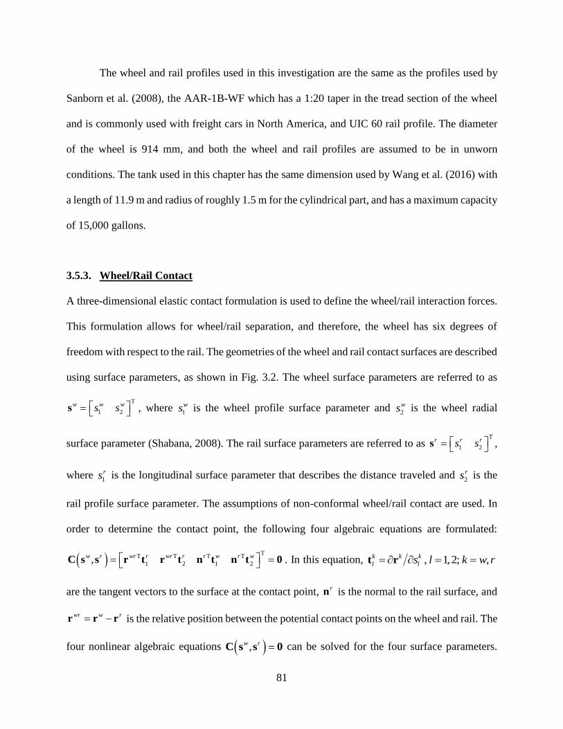
81
The wheel and rail profiles used in this investigation are the same as the profiles used by
Sanborn et al. (2008), the AAR-1B-WF which has a 1:20 taper in the tread section of the wheel
and is commonly used with freight cars in North America, and UIC 60 rail profile. The diameter
of the wheel is 914 mm, and both the wheel and rail profiles are assumed to be in unworn
conditions. The tank used in this chapter has the same dimension used by Wang et al. (2016) with
a length of 11.9 m and radius of roughly 1.5 m for the cylindrical part, and has a maximum capacity
of 15,000 gallons.
3.5.3. Wheel/Rail Contact
A three-dimensional elastic contact formulation is used to define the wheel/rail interaction forces.
This formulation allows for wheel/rail separation, and therefore, the wheel has six degrees of
freedom with respect to the rail. The geometries of the wheel and rail contact surfaces are described
using surface parameters, as shown in Fig. 3.2. The wheel surface parameters are referred to as
T
1 2
w w ws s = s , where 1
ws is the wheel profile surface parameter and 2
ws is the wheel radial
surface parameter (Shabana, 2008). The rail surface parameters are referred to as T
1 2
r r rs s = s ,
where 1
rs is the longitudinal surface parameter that describes the distance traveled and 2
rs is the
rail profile surface parameter. The assumptions of non-conformal wheel/rail contact are used. In
order to determine the contact point, the following four algebraic equations are formulated:
( )T
T T T T
1 2 1 2,w r wr r wr r r w r w = = C s s r t r t n t n t 0 . In this equation, , 1,2; ,k k k
l ls l k w r= = =t r
are the tangent vectors to the surface at the contact point, r
n is the normal to the rail surface, and
wr w r= −r r r is the relative position between the potential contact points on the wheel and rail. The
four nonlinear algebraic equations ( ),w r =C s s 0 can be solved for the four surface parameters.

82
These four surface parameters are used to define the potential contact points on the wheel and rail.
The wheel/rail penetration and the relative velocity along the normal to the rail are defined,
respectively, as Twr r = r n and
Twr r = r n . If there is a penetration between the wheel and rail, an
elastic force model is used to define the normal force (Shabana, 2008). The normal force, the
creepages, the dimensions of the contact ellipse, and the wheel and rail material properties are used
to define the tangential creep force and spin moment using Kalker’s USETAB subroutine (Kalker,
1990). The dimensions of the contact ellipse are determined using Hertz’s contact theory which
requires the evaluation of the principal curvatures. It is also important to point out that the
nonlinear algebraic equations ( ),w r =C s s 0 are used only to determine the geometric surface
parameters and there are no constraint forces associated with these algebraic equation since
wheel/rail separation is allowed. More details on the elastic contact formulation used in this study
can be found in the literature (Shabana, 2008).
3.5.4. MBS Equations of Motion
The general equations of motion for an MBS system that consists of rigid and flexible bodies,
including bodies modeled using the ANCF formulation, can be written in terms of the rigid body
reference coordinates rq , ANCF nodal coordinates e , and the non-generalized surface parameters
s used in the contact formulations, as (Shabana, 2005; Shabana, 2013)
r
r
r rr
ee
d
=
q
e
s
q e s
M 0 0 C Qq
Qe0 M 0 C
0s0 0 0 C
QλC C C 0
(3.10)
83
where rq , e , and s are, respectively, the second time derivatives of the reference, ANCF, and
non-generalized coordinates; rM and eM are, respectively, the rigid body mass matrix and ANCF
constant mass matrix; rqC , eC , and sC are the Jacobian matrices of the constraint equations
associated, respectively, with the reference, ANCF, and non-generalized coordinates; λ is the
vector of Lagrange multipliers; rQ and eQ are, respectively, the vectors of generalized forces
associated with the rigid and elastic coordinates, and dQ is the quadratic velocity vector that
results from the differentiation of the nonlinear algebraic constraint equations twice with respect
to time. The numerical procedure used in this chapter ensures that the nonlinear algebraic
constraint equations are satisfied at the position, velocity, and acceleration levels. A flowchart
depicting the numerical solution procedure is shown in Fig. 3.10.
3.6. Numerical Simulations
In the numerical investigation presented in this section, the effect of liquid sloshing on the vehicle
dynamics is examined. Simulations of a vehicle negotiating a curved track are performed in order
to evaluate the wheel/rail contact forces and the movement of the center of mass of the tank and
fluid, and to have a better understanding of the effect of liquid sloshing on vehicle dynamics when
the vehicle forward velocity is varied. The traction and braking scenarios on a tangent track are
also considered in order to examine the load transfer between the two trucks and the coupler forces
between the two vehicles. These braking scenarios are used to evaluate the effect of liquid sloshing
on the performance of the ECP brake system. The numerical results obtained in this chapter show
that the liquid sloshing does not have a pronounced effect on the vehicle critical speed, but it does
affect the change of the wheel load when the vehicle negotiates a curve at a velocity different from
the balance speed. In the case of vehicle traction and braking, there is significant fluid motion due

84
Figure 3.10. Flowchart of the numerical solution procedure

85
to the acceleration and deceleration of the vehicle. The numerical results are obtained in this
section using tanks partially filled with water.
3.6.1. Curve Negotiation and Balance Speed Analysis
In this section, the curved track described in Table 3.1 is used to investigate the effect of liquid
sloshing on vehicle dynamics by evaluating the wheel/rail contact forces and the movement of the
center of mass of the tank and fluid when the vehicle forward velocity is varied. The track has a
radius of curvature of roughly 582 m which results in a balance speed of roughly 63 km/h defined
in the case of rigid body dynamics as tV gRh G= , where g is the gravity constant, R is the
radius of curvature of the curve, th is the super-elevation, and G is the track gauge. In order to
examine the impact of liquid sloshing on curve negotiation, forward velocities of 40 km/h, 60 km/h,
and 90 km/h are considered in this chapter.
3.6.1.1. Centrifugal Forces
The effect of the centrifugal force when a vehicle is negotiating a curve is to push the vehicle
outward along the direction normal to the curve. The inertia forces of the fluid can be expressed
as the product of the acceleration of the center of mass and the total mass. In order to obtain the
centrifugal force of the fluid and analyze its longitudinal motion, the normal and tangent vectors
can be determined by using the transformation matrix of the track frame relative to the tank body
(Shabana, 2008).

86
Figure 3.11. Lateral component of gravity and outward inertia forces of the fluid
( Gravity force, 40km/h, 60km/h, 90 km/h)
Figure 3.11 shows the outward inertia force and the lateral component of gravity force of
the fluid, which is due to the super-elevation of the track. In order to plot the curves at various
velocities in one figure, the traveling time along the curve is normalized to a dimensionless
parameter which represents the curve length. The results presented in this figure show that the
centrifugal force exerted on the fluid is smaller than the lateral component of the gravity force
when the vehicle travels below the balance speed; however, a larger centrifugal force is exerted
when the vehicle speed is above the balance speed. The resultant force can affect the tank motion
as shown in Fig. 3.12 in which the lateral displacement of the geometric center of the tank with
respect to the track is plotted for both the fluid and rigid body models at various velocities. This
figure illustrates that the liquid sloshing can exacerbate the unbalanced effects when the vehicle
negotiates a curve at a velocity away from the balance speed. It can also be found that when the
vehicle travels near the balance speed, there are no significant differences between the fluid and

87
rigid body model since the liquid exerts the same magnitude of centrifugal force as the lateral
component of gravity, as seen in Fig. 3.11. Traveling at a speed greater than the balance speed
causes instability, which is evident by the results presented in Fig. 3.12c, where the oscillations of
the rigid body model increase after the first curve. However, due to the damping effect of the liquid
motion, the fluid model experiences increased stability compared to the rigid body model.
(a) (b)
(c)
Figure 3.12. Position of the tank center with respect to the track in the lateral direction at (a)
40km/h, (b) 60 km/h, and (c) 90 km/h ( Rigid, Fluid)
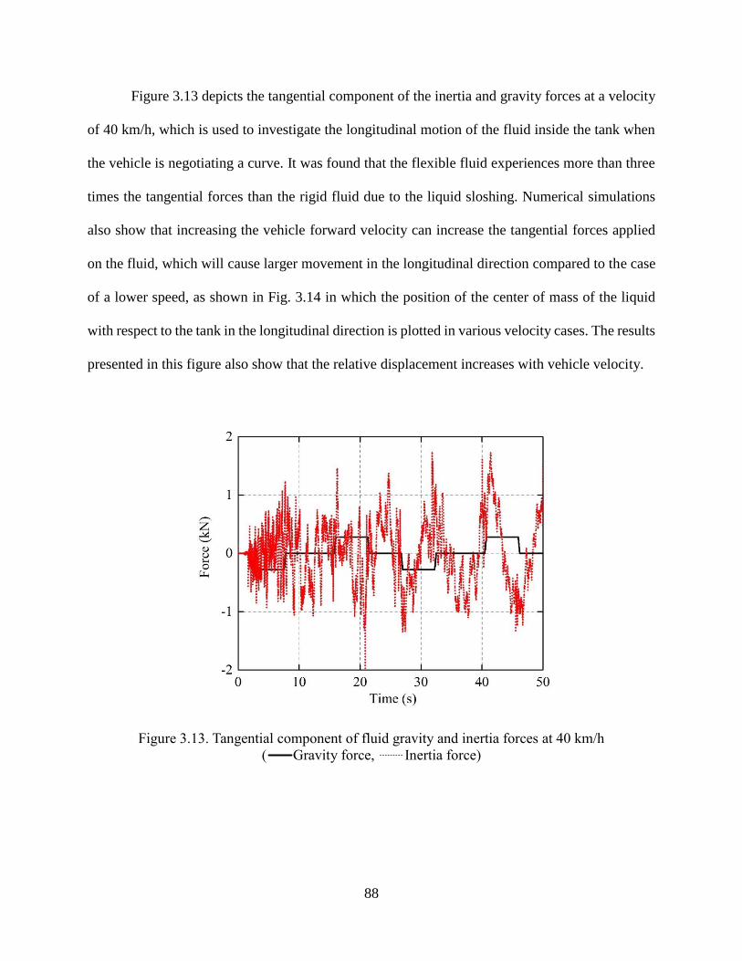
88
Figure 3.13 depicts the tangential component of the inertia and gravity forces at a velocity
of 40 km/h, which is used to investigate the longitudinal motion of the fluid inside the tank when
the vehicle is negotiating a curve. It was found that the flexible fluid experiences more than three
times the tangential forces than the rigid fluid due to the liquid sloshing. Numerical simulations
also show that increasing the vehicle forward velocity can increase the tangential forces applied
on the fluid, which will cause larger movement in the longitudinal direction compared to the case
of a lower speed, as shown in Fig. 3.14 in which the position of the center of mass of the liquid
with respect to the tank in the longitudinal direction is plotted in various velocity cases. The results
presented in this figure also show that the relative displacement increases with vehicle velocity.
Figure 3.13. Tangential component of fluid gravity and inertia forces at 40 km/h
( Gravity force, Inertia force)

89
Figure 3.14. Liquid center of mass with respect to the tank in the longitudinal direction
( 40km/h, 60km/h, 90 km/h)
3.6.1.2. Wheel/Rail Contact Forces
The wheel/rail contact forces are also examined in the case of the vehicle negotiating a curve and
are used to examine the impact of the liquid sloshing on wheel/rail interaction. Figures 3.15 and
3.16 depict the normal contact forces on the tread and flange, respectively, on both left and right
wheels of the lead wheelset of the lead truck. The normal forces on the tread show that the liquid
sloshing can intensify the load variance on both the right and left wheels, and tends to increase the
amount of the load variation when the vehicle does not travel at the balance speed during the curve
negotiation case. However, the normal forces on the flange increase with the vehicle forward
velocity and there are no noticeable differences between the fluid and rigid body models.

90
(a) (b)
(c)
Figure 3.15. Tread normal contact force of truck lead wheelset (a) 40km/h, (b) 60 km/h, (c) 90
km/h. ( Rigid-Right, Fluid-Right, Rigid-Left, Fluid-Left)
(a) (b)

91
(c)
Figure 3.16. Flange normal contact force of truck lead wheelset (a) 40km/h, (b) 60 km/h, (c) 90
km/h. ( Rigid-Right, Fluid-Right, Rigid-Left, Fluid-Left)
Figures 3.17 and 3.18 depict the lateral contact forces on the tread and flange, respectively,
which exhibit similar patterns compared to the normal forces. It is clearly shown that the lateral
forces on the flange increase with the vehicle forward velocity since more lateral forces are needed
to balance the centrifugal forces, which also increase with the vehicle velocity.
(a) (b)

92
(c)
Figure 3.17. Tread lateral contact force of lead wheelset of lead truck (a) 40km/h, (b) 60 km/h,
(c) 90 km/h. ( Rigid-Right, Fluid-Right, Rigid-Left, Fluid-Left)
(a) (b)
(c)
Figure 3.18. Flange lateral contact force of lead wheelset of lead truck (a) 40km/h, (b) 60 km/h,
(c) 90 km/h. ( Rigid-Right, Fluid-Right, Rigid-Left, Fluid-Left)

93
3.6.2. Traction and Braking Analysis
In this section, motion scenarios are used to examine the impact of liquid sloshing on the vehicle
nonlinear dynamics in the traction and braking cases.
3.6.2.1. Vehicle Traction Analysis
Figure 3.19. Average normal contact forces of lead and rear trucks in the traction case
( Rigid-Lead, Fluid-Lead, Rigid-Rear, Fluid-Rear)
In the traction scenario, a single vehicle model is used and a trajectory velocity constraint is applied
on the lead stub sill to represent the vehicle traction scenario. The trajectory velocity constraint
causes the vehicle to accelerate according to user-specified trajectory and velocity relationships
(Shabana, 2008). A constant acceleration of 0.3 m/s2 is used to accelerate the vehicle to 20 km/h
in 15 s and then maintain this constant velocity. The average contact forces of the four wheels of
the lead and rear trucks are plotted in Fig. 3.19. It is evident that the liquid sloshing has a significant
effect on the load distribution during the vehicle traction; there is an approximately 13% difference
in the normal load compared with that of the rigid body model. After traction, the liquid continues

94
to experience sloshing towards a steady state which can be clearly seen in Fig. 3.20, which shows
the longitudinal displacement of the fluid center of mass with respect to the tank during the traction.
It is apparent that there is a maximum motion of roughly 0.7 m of the center of mass, which will
certainly affect the wheel load as shown in Fig. 3.19.
Figure 3.20. Fluid center of mass longitudinal displacement with respect to the tank in the
traction case
3.6.2.2. Vehicle Braking Analysis
(a) (b)
Figure 3.21. Coupler forces between two cars in the case of braking using (a) Conventional
brake, (b) ECP brake ( Rigid, Fluid)

95
In order to consider the coupler force between cars, a two tank-car model is developed based on
the single MBS vehicle model to simulate the braking scenarios, in which the coupler is
represented as a linear spring-damper force element. The nonlinear braking torque associated with
the vehicle loads and forward velocities is applied on the wheelsets to perform braking in this
analysis. The case where only the lead car brakes as well as the case where both cars brake are
simulated in order to consider the usual brake situations. These two scenarios are used to examine
the effects of liquid sloshing on the dynamic response of the train during braking when the
conventional and ECP brake systems are used. In this chapter, the train is decelerated from 40
km/h to 5 km/h in 40s with a nonlinear braking force. The coupler used in this model has a stiffness
coefficient 300 MN m and a damping coefficient of 200 kN s m . The coupler forces are plotted
in Fig. 3.21 in the case where only the lead car brakes as well as the case of both cars braking, for
both the fluid and rigid body models. By comparing the results in Figs. 3.21a and 3.21b, it can be
seen that a larger coupler force is exerted when only the lead car brakes regardless of whether the
flexible fluid or the equivalent rigid fluid model is used, which shows the significance of ECP
application in railroad vehicles. In the case of brake application on the lead car only, the flexible
fluid model has essentially the same coupler force as that of the rigid fluid model initially, while
it experiences a larger value as the vehicle velocity decreases. However, in the case of uniform
and simultaneous brake application on both cars (ECP), the flexible fluid model shows
significantly larger coupler forces than the rigid body model for the entire scenario due to the
increased relative motion of the fluid inside the tank as shown in Fig. 3.22, which depicts the
longitudinal and lateral displacement of the center of mass of the fluid with respect to the tank. It
is clearly shown that in the case of ECP braking, the fluid moves more significantly because the
vehicle system experiences a more severe acceleration resulting from increased braking torques

96
that are applied as compared to the conventional brake scenario. Figure 3.23 shows the
configuration of these two cars partially filled with water in braking, and it can be clearly seen that
there is significant liquid motion due to the deceleration of the vehicle.
(a) (b)
Figure 3.22. Front car fluid center of mass displacement with respect to the tank during braking
(a) Longitudinal, (b) Lateral direction ( Conventional brake, ECP brake)
(a)
(b)
Figure 3.23. Braking animation of two tank-cars filled with liquid in the (a) Parked state, (b)
Braking state

97
3.7. Concluding Remarks
In this chapter, a new approach is proposed for the integration of a continuum-based sloshing
model with a fully nonlinear MBS rail vehicle model. The contributions of this chapter are as
follows: (1) A unified geometry/analysis mesh is used from the outset in order to accurately capture
complex fluid and tank geometries as well as the nonlinear dynamic behavior of the fluid and
vehicle. The approach developed in this chapter is used to examine the effects of liquid sloshing
on railroad vehicle dynamics when negotiating a curve and during traction or braking; (2) The
method of the tank and fluid geometry description is described and it is shown how a unified
geometry/analysis mesh can be developed for both the rigid rail and continuum fluid bodies. The
search method used to define the fluid/tank contact points is outlined and the penalty force model
used to describe the fluid/tank interaction forces is formulated; (3) The fluid constitutive equations
that account for the viscosity and incompressibility effects are presented. The liquid sloshing
model developed in this study is integrated with the MBS railroad vehicle model which takes into
consideration the nonlinear three-dimensional wheel/rail contact forces and the wheel and rail
profile geometries; and (4) In order to systematically examine the effect of the motion of the
flexible fluid on railroad vehicle dynamics when the vehicle is negotiating a curve, a general
definition of the outward inertia force of a flexible body using both FFR and ANCF descriptions
is investigated. The analysis presented in this chapter shows that this force depends strongly on
the motion of the continuum and does not take the simple form used in the case of rigid body
dynamics.
Comparative simulations are performed to examine the liquid sloshing effects by using
flexible and rigid body fluid models. It is shown that the liquid sloshing can exacerbate the
unbalanced effects when the vehicle travels at a velocity away from the balance speed, but this

98
effect decreases when the forward velocity is close to the balance speed because the liquid
experiences the same centrifugal force as the rigid fluid body in this case. The results in the traction
analysis show that the liquid motion can significantly affect the load distribution between the front
and rear trucks. Comparing with the ECP braking case, there is a larger coupler force when the
conventional braking is used for both the flexible and rigid body fluid models. Nonetheless, the
results obtained for the model considered in this chapter demonstrate that the liquid sloshing
amplifies the coupler force greatly in the ECP braking case compared to the equivalent rigid body
model because the latter model cannot capture the fluid nonlinear inertia effects.

99
CHAPTER 4
GEOMETRICALLY ACCURATE REDUCED ORDER FLUID MODELS
The objective of this chapter is to integrate for the first time the newly developed absolute nodal
coordinate formulation/floating frame of reference (ANCF/FFR) solid finite elements (FE) with a
fully nonlinear multibody system (MBS) algorithm. ANCF/FFR elements are able to capture
initially curved structures such as the fluid within a cylindrical tank while retaining the same
number of degrees of freedom as conventional elements and taking advantage of modal reduction
techniques, resulting in faster simulation times compared to the higher-order ANCF elements. In
this chapter, the solid element is developed in terms of constant geometric coefficients which are
obtained using the matrix of position vector gradients defined in the reference configuration. No
geometry distortion occurs when computer-aided design (CAD) models are converted to FE
meshes using ANCF/FFR elements because such meshes are developed using ANCF elements,
which are related to B-splines and Non-Uniform Rational B-Splines (NURBS) by a linear mapping.
The fluid constitutive model, which is based on the Navier-Stokes fluid model, is developed and
the incompressibility conditions, which are enforced using a penalty approach, are defined. A
sloshing box model and a medium-duty tanker truck model with a tank half filled with water are
developed in order to investigate the ability of the new ANCF/FFR elements to model the fluid
sloshing in comparison to fluid meshed using ANCF elements. The fluid/tank contact formulation,
which is enforced using a penalty approach, is described. It is shown that while the sloshing
amplitudes of the ANCF/FFR box meshes are reduced compared to the converged ANCF meshes,
the general sloshing behavior is still captured at a significantly reduced CPU time, indicating that

100
the ANCF/FFR elements can contribute to significant improvement of the computational
efficiency in applications in which capturing some geometric changes due to the fluid displacement
is not critical. This conclusion was confirmed by the results of the highway vehicle lane change
simulation – the sloshing amplitudes of the center of mass predicted using the ANCF/FFR fluid
mesh during the lane change are found to be in a good agreement with what predicted by the ANCF
mesh. Furthermore, the results of the overall vehicle-dynamics, as measured by the tire contact
forces predicted using the two different meshes, are found to be in a good agreement. The results
obtained in this investigation demonstrate that if the goal is to accurately capture the free-surface
displacement of the fluid, then ANCF elements are better candidates due to their high order and
ability to capture complex shapes. However, if the goal is to perform efficient simulations to obtain
the overall vehicle motion, then using ANCF/FFR elements are a better alternative.
4.1. FE Mesh Geometry and Position Vector Gradients
Figure 4.1. Cylindrical vehicle tank
The tanker truck considered in this investigation features a tank with cylindrical geometry, as
shown in Fig. 4.1. It is necessary for the FE mesh to have an accurate representation of the initially

101
curved geometry in order to develop a realistic virtual model in which the fluid fills the tank. In
this section, the method used to produce the initially curved reference-configuration geometry of
the ANCF and ANCF/FFR meshes used to model the fluid inside the tank is described. The fluid
body can be described using three different configurations, as depicted in Fig. 4.2. The curved
reference configuration is the initial configuration of the fluid inside the tank at the start of the
simulation. Its volume is denoted as oV with position vector X . The initially curved reference
configuration is achieved by shaping a straight configuration, with volume V and position vector
x . During the simulation, the fluid may experience large deformations due to the forces exerted
by the tank. These deformed shapes are referred to as the current configuration, with volume v
and position vector r . The volumes of the curved reference and current configurations are related
by the determinant of the matrix of position vector gradients = J r X according to odv JdV= ,
where J = J and denotes the determinant of a matrix. The curved reference configuration is
related to the straight reference configuration by o odV J dV= .
Figure 4.2. Fluid configurations

102
Furthermore, the mesh in the current configuration can be mapped to the straight reference
configuration; by rewriting the matrix of position vector gradients as
( )( ) 1
e o
−= = =J r X r x x X J J , where eJ relates the volumes in the current and straight
reference configurations, one can write 1
o o e o o edv JdV JJ dV J dV J dV−= = = =J J . Using these
identities, integrations carried out over the curved configurations can be systematically converted
to integrations over the straight reference configuration, regardless of the amount of deformation
that occurs within the fluid mesh.
The ANCF/FFR solid element is developed using the ANCF solid element as a basis, which
features eight nodes with three gradient vectors and three absolute position coordinates, for a total
of 12 coordinates per node and 96 coordinates per element (Olshevskiy et al., 2013). The cubic
shape functions allow for the creation of complex geometries, such as a half-cylindrical fluid mesh
which can be coincident with the tank walls. The shape functions ( )1,2,3,4k
is i = at node
( )1,2, ,8k k = for this element are as follows:
( ) ( )( )( )( )( ) ( )( ) ( )( )( )
( ) ( ) ( ) ( )
( ) ( ) ( ) ( )
( ) ( ) ( ) ( )
1
1
2 1 11
2
1 2 11
3
1 1 21
4
1 1 1 1
1 1 2 1 2 1 2
1 1 1 1
1 1 1 1
1 1 1 1
k k k
k k k k kk k k
k k k k kk k k
k k k k kk k k
k
k k k
k k k
k
k
k
s
s a
s b
s c
+ + +
+ − − −+
+ − − −+
+ − − −+
= − + − + − + −
+ + − + − − + − −
= − − − −
= − − − −
= − − − −
(4.1)
where , , and are the dimensionless parameters along the three coordinate axes, and k ,
k , and k are the parameters evaluated at node k . The mesh in the straight reference
configuration can be shaped into a half-cylinder by adjusting the gradient vectors at each node.
More information about using the gradients to develop initially curved meshes can be found in the
literature (Shi et al., 2017).

103
The ANCF/FFR solid element also features eight nodes, however the nodal coordinate
vector includes infinitesimal rotations and a local position vector, instead of the gradient vectors
and absolute position vector used by ANCF elements (Shabana, 2018; Tinsley and Shabana, 2019).
The transformation from gradient vectors to infinitesimal rotations and the derivation of the new
shape function matrix will be described in the following section.
4.2. Finite Element Formulations
In this section, the ANCF formulation, the conversion of nodal gradient vectors to infinitesimal
rotations, and the FFR formulation are described.
4.2.1. Absolute Nodal Coordinate Formulation
The position of an arbitrary point on an ANCF body can be written as
( ) ( ) ( ) ( ) ( )( ), o dt t t= = +r x S x e S x e e , where ( )S x is the space-dependent shape function matrix,
e is the time-dependent vector of nodal coordinates defined in the current configuration, oe is the
vector of nodal coordinates in the curved reference configuration, and de is the vector of
deformation coordinates, where o d+e = e e and the nodal coordinates are defined in the global
coordinate system. Using general continuum mechanics, the position vector can be rewritten as
o d= +r r r , where or is the position of the point in the curved reference configuration and dr is
the displacement vector, and thus o o=r Se and d d=r Se , demonstrating that ANCF elements are
isoparametric. The matrix of position vector gradients which relates the current and curved
reference configurations can be written as 1
e o= −J J J , where o o= = xJ X x S : e ,
e r= = xJ x S : e , xS is a third-order tensor defining the derivatives of the shape functions with

104
respect to the coordinates in the straight reference configuration, and : denotes the tensor double
contraction. The velocity and acceleration equations are obtained by differentiating the position
equation once and twice, respectively, with respect to time and can be written as =r Se and
r = Se . Using the velocity equation, the kinetic energy can be defined as
( ) ( ) ( ) ( )1 2 1 2 1 2T T T T
v vT dV dV = = = r r e S S e e Me , where
T
vM dV= S S is the constant,
symmetric mass matrix. The ANCF generalized external forces can be obtained using the principal
of virtual work. The virtual work of the external forces can be written as
T T T
e fW = = =F r F S e Q e , where T
f =Q S F is the vector of generalized forces associated
with the ANCF elastic coordinates.
4.2.2. Conversion of Position Vector Gradients to Infinitesimal Rotations
The matrix of position vector gradients for the ANCF/FFR elements can be written as
( )1 2 3, ,e o o = =J JJ A J , where A is an orthogonal rotation matrix which is a function of the
three rotation parameters 1 , 2 , and 3 and can be written as
( ) ( ) ( )1 1 2 3 2 1 2 3 3 1 2 3, , , , , ,= = A J a a a where the columns ia ( )1,2,3i = are
orthogonal unit vectors. Using the assumption of infinitesimal rotations, the rotation matrix A can
be written as = +A I θ , where θ is a skew-symmetric matrix associated with the vector of rotation
coordinates 1 2 3
T =θ . Substituting this equation into the equation for the matrix of
position vector gradients eJ yields ( )e o o o o= = + = +J AJ I θ J J θJ . This equation can be
rewritten as
1 2 3 1 2 3 1 2 3e o o o o o o o o o o o o = + = + = + − − − J J θ J J J J θJ θJ θJ J J θ J θ J θ where

105
( )1,2,3oi i =J are the skew-symmetric matrices associated with the column vectors ( )1,2,3oi i =J
of oJ . Thus, the vector of element nodal coordinates which includes position vectors and position
vector gradients can be written as
( ) ( ) 1 1 1
2 2 2
3 3 3
o
x o o d
o d o cd
x o o
x o o
t t
− = + = = + = + −
−
r r I 0
r J 0 J re e e e Be
r J 0 J θ
r J 0 J
(4.2)
where 0
k k
cd=e Be . At an arbitrary node k , the nodal coordinates can be written as
( )k k k k k
o d o cdt = + = +e e e e Be , where
( ) ( )1
2
3
11
22
33
; ; ;
k k
ok kk kx ok k k ko d
o cdk kk kx oo
kkkoox
t t
− = = = = − −
r I 0r
r 0 JJ re e B e
r 0 JJ θ
0 JJr
(4.3)
Recalling from Sec. 4.2.1 that the position of an arbitrary point on the ANCF body can be
written as ( ) ( ) ( ) ( )( )o d= t t= +r S x e S x e e , one can substitute Eqn. (4.1) into this position
equation to yield ( ) ( ) ( ) ( )( )o cd o d cd= t t= + = +r S x e S x e Be Se S e where d =S SB is the new
displacement shape function matrix. This demonstrates that the new ANCF/FFR-FEs are non-
isoparametric elements, because different shape functions are used to interpolate the geometry and
displacements; however, the effect of the initial curved geometry is still accounted for in the shape
functions dS and the position equation can be used for both straight and curved geometries. It can
also be shown that the displacement shape function matrix has a proper set of rigid body modes at
the velocity level (Shabana, 2017B), which is important because the velocity equation is used to
define the element inertia, which will be shown in the following section. The displacement

106
shape function matrix for node k ( )1,2,...,8k = can be written as
4 3 4 2 4 1 4
1 2 3( )k k k k k k k k k k
d o o oS S S S− − − = = − + + S S B I J J J and can be assembled at the element level
as 1 2 8
d d d d = S S S S .
4.2.3. Floating Frame of Reference Formulation
The position vector i
Pr to an arbitrary point P on a flexible body i , as shown in Fig. 4.3, can be
written in the FFR formulation as i i i
P P= +r R u , where i
R is the global position vector to the body
coordinate system and i
Pu is the global position of point P with respect to the body coordinate
system. i
Pu can also be written i i i
P P=u A u , where i
A is the orthogonal transformation matrix
which describes the orientation of the body reference system, and i
Pu is the local position vector
to point P in the body coordinate system. In the FFR formulation, the local position vector i
Pu
can be decomposed as i i i
P O f= +u u u , where i
Ou is the position vector to point P in the reference
configuration, and i
fu is the local deformation vector. i
fu can be written as i i i
f f=u S q , where i
S
is the shape function matrix of body i , and i
fq is the vector of the FFR elastic coordinates. Thus,
the global position vector of point P is ( )i i i i i i
P O f= + +r R A u S q .
Figure 4.3. Floating Frame of Reference formulation

107
The velocity equation can be obtained by differentiating the position equation with respect
to time, and by knowing that i
Ou and i
S are constant with respect to time. The velocity of point P
can therefore be written as i i i i i i i
P P f= + +r R A u A S q . In the preceding equation, the first term is the
velocity of the body reference and the third term is the velocity of point P due to local deformation.
The second term results from differentiation of the rotation matrix with respect to time and is equal
to zero in the case of rigid body motion. The second term can be written as
( ) ( )i i i i i i i i i i i i i i i i i
P P P P P= = − = − = − =A u A ω u A u ω Au ω Au G θ Bθ , where i
G is the velocity
transformation matrix which relates the angular velocities i
ω and the time derivatives of the
coordinates iθ , and i i i i
P= −B A u G . This partitioning allows for writing the velocity equation in
matrix form as
i
i i i i i
p
i
f
=
R
r I B A S θ
q
(4.4)
where I is a 3x3 identity matrix. Defining the left-hand matrix as i
L , the velocity equation can be
written in simple form as i i i
P =r Lq , where i i i i = L I B A S and T T T T
i i i i
f =
q R θ q is the
vector of generalized velocities.
To obtain the acceleration vector, the matrix form of the velocity equation is differentiated
with respect to time as i i i i i
P +=r Lq Lq . In the preceding equation, the first term includes quantities
which are quadratic in the velocities, such as the Coriolis terms, and the second term includes
quantities linear in the accelerations. It can also be shown that this equation may be written as
( ) ( )2i i i i i i i i i i i i i i i i i
P P P P P O N T C D= + + + + = + + + +r R ω ω u α u ω Au A u a a a a a , where i
Oa is the
acceleration of the body reference, i
Na is the normal component of the acceleration, i
Ta is the

108
tangential component, i
Ca is the Coriolis component, and i
Da is the acceleration due to the local
deformation. It is clear that in the case of rigid body motion, the last two terms are equal to zero
because i
Pu is constant.
Using the velocity equation that was previously defined, the kinetic energy can be written
as ( ) ( )1 2 1 2T T T
i i
i i i i i i i i i i i
V VT dV dV = = r r q L Lq . Because the velocities are not a function of
the volume, this equation can be written as ( ) ( )1 2 1 2T T T
i
i i i i i i i i i i
VT dV= =q L L q q M q where
T
i
i i i i i
VdV= M L L is the symmetric positive definite mass matrix of body i . The mass matrix
can be partitioned as
.
i i i
RR R Rf
i i i
f
i
ffsym
=
m m m
M m m
m
(4.5)
where
T
T T
i i i i i i i
RR RV V
i i i i i i i i i
RfV V
i i i i i i i i i i i
f ffV V
dV dV
dV dV
dV dV
= =
= =
= =
m I m B
m S m B B
m B A S m S S
(4.6)
It is clear that i
RRm and i
ffm are constant with respect to time; in general, however, the FFR mass
matrix is highly nonlinear and varies with time.
The virtual work of the generalized external forces acting on body i , including the gravity
force and the tank contact, can be written as T Ti i i i
e e fW = =F r Q q , where i
F is the external force
vector, ir is the virtual change in the position vector, and
T T T Ti i i i
e R f =
Q Q Q Q is the vector
of generalized external forces; i i
R =Q F and ( )T
i i i i i
P = −Q A u G F are the vectors of generalized

109
forces associated with the reference translation and rotation, respectively, and ( )T
i i i i
f =Q A S F is
the vector of generalized forces associated with the deformation.
4.3. Fluid Modeling Approaches
In this thesis, the fluid in the vehicle tank is assumed to be water. The constitutive model and the
method for enforcing the fluid incompressibility are discussed in this section.
4.3.1. Fluid Constitutive Model
The constitutive model used in this chapter is based on the Navier-Stokes equations and is
applicable to Newtonian fluids; in this thesis, water is the fluid considered. This constitutive model
has been validated against experimental and numerical techniques and found to be in good
agreement (Grossi and Shabana, 2017). The fluid equations can be defined by the symmetric
Cauchy stress tensor as ( )tr 2 vol devp = − + + = + σ D I D σ σ , where p is related to the
hydrostatic pressure, ( )tr refers to the trace of a matrix, D is the rate of deformation tensor, I is
a 3x3 identity matrix, and and are the Lamé constants.
Because the penalty approach is used to enforce the incompressibility in this investigation,
as will be discussed in the following section, the first two terms of the stress tensor vanish, reducing
to 2dev dev=σ D . The second Piola-Kirchoff stress tensor is defined in the reference configuration
and is therefore often used in Lagrangian analysis. The second Piola-Kirchoff stress tensor can be
obtained from the Cauchy stress tensor as 1
2
T
P devJ − −=σ J σ J , where X Y X= =J r X r r r is
the matrix of position vector gradients, X is the vector of coordinates in the curved reference
configuration, and J=J , as defined previously. The virtual work of the fluid viscous forces for

110
an element j can be written as ( )0
1
2 0: :jj
j j j j j j j j
s dev Pv V
W dv dV −
= − = − σ J J σ ε where
( )( )1 2Tj j j= −ε J J I is the Green-Lagrange strain tensor,
jv is the volume of element j in the
current configuration, 0
jV is the volume of element j in the curved reference configuration, and
: indicates the double contraction. Using the expression for 2Pσ and the identity
( ) ( )1T
j j j− −
=D J ε J , the virtual work of the viscous forces becomes
( ) ( )0
1 1
02 :T
j
j j j j j j
s r r vV
W J dV − −= − = C εC ε e Q e , where
( ) ( )0
1 1
02 :j
j j j j j
v r rV
J dV − −= − Q C εC ε e is the vector of generalized viscous forces and j
e are
the nodal coordinates of element j . By using the identity 1 1
0 0
j j j j j j
e eJ− −
= = =J J J J J , the vector
of generalized viscous forces can be rewritten as
( ) ( ) ( ) ( )0
1 1 1 1
02 : 2 :j j
i j j j j j j j j j j
v r r r rV V
J dV J dV − − − −= − = − Q C ε C ε e C ε C ε e (4.7)
This allows for carrying out integration in the straight reference configuration, which is constant
in time.
4.3.2. Fluid Incompressibility
In the case of incompressible fluids such as water, the fluid incompressibility can be enforced
using one of several methods. The continuity condition ( )( ) ( )( ), t t +r r reduces to
0 =r in the case of incompressible materials, where is the density of the fluid, because for
incompressible fluids, the density is constant over both space and time. This constraint equation
can be applied at each integration point to ensure the fluid remains incompressible. However, this
method introduces a significant number of constraint equations, thus reducing the computational

111
efficiency of the model. Therefore, in this chapter, the penalty approach is instead used again to
enforce the incompressibility. The incompressibility condition is enforced at both the position
( )1jJ = and velocity ( )0jJ = levels using the energy function ( ) ( )2
1 2 1j j j
C CU k J= − and the
dissipation function ( ) ( )2
1 2j j j
D DU c J= , respectively. The penalty coefficients are chosen such
that jJ remains within a specified tolerance of 1. The generalized forces associated with
incompressibility of element j can be defined as ( ) ( )( )1Tj j j j j j j
C C CU k J J= = − Q e e at the
position level and ( ) ( )Tj j j j j j j
C D DU c J J= = Q e e at the velocity level, where
j j j jJ J = e e and ( )trj j jJ J= D . By using the identity
( ) ( ) ( )j j j j j j j j j j
X Y Z Y Z X Z X YJ = = = r r r r r r r r r , any of the three expressions can be used to
calculate j jJ e as ( ) ( ) ( )j j j j j j j j j j j
X Y Z Y Z X Z X YJ = + + e S r r S r r S r r . The generalized
forces on body j , j j j j
v C D= + +Q Q Q Q , can be assembled using a standard finite element assembly
procedure to determine the generalized forces acting on the fluid body.
4.4. Fluid/Tank Contact
In this section, the contact detection algorithm between the fluid and tank will be developed. The
contact is checked in two directions – radially in the cylindrical section and longitudinally for the
flat tank ends. The contact forces, based on the penalty approach, will also be discussed for the
case of an ANCF/FFR or ANCF fluid body.

112
4.4.1. Contact Detection
Consider a point P on the fluid body, which is located at position Pr in the global frame. In order
to determine if contact between fluid point P and the tank is occurring, the global position of
point P with respect to the tank coordinate system is obtained by
1 2 3
Tt t t t t
P P P P Pu u u = = − u r R , where t
R is the position vector to the tank coordinate system.
The position vector of the point P relative to the tank coordinate system is transformed to the
local coordinate system using the matrix t
A which defines the orientation of the tank coordinate
system as Tt t
P P=u A u . Contact is detected separately in the radial direction in the cylindrical
portion of the tank, and in the longitudinal direction at the tank ends.
4.4.1.1. Radial Direction
The longitudinal direction of the tank is along the X axis of the tank coordinate system, and thus
radial contact is checked in the local Y Z− plane. In order to detect contact in this plane, the
projection matrix P is defined as ˆ ˆ= − P I a a , where a is a unit vector along the tank
longitudinal axis. The projection of the local position vector t
Pu is thus calculated as ( )t t
P Pr=u Pu ,
which is the position of the fluid point in the radial plane. Given that the radius of the tank is tr ,
contact is occurring between point P and the tank if the length of ( )t
Pr
u exceeds the tank radius,
or if ( ) ( ) ( )t t t t
P P Pr r r
r= u u u , and the amount of penetration can be calculated as
( )t t
Pr
r r = −u . The unit normal vector along which the penalty force acts is defined as
( ) ( )t t
r P Pr r
= −n u u .

113
4.4.1.2. Longitudinal Direction
The vehicle tank features flat ends, and thus contact is detected by comparing the position of the
fluid point relative to the tank’s length. The local position vector of point P in the tank coordinate
system is projected on a unit vector along the tank’s length, that is ( ) ˆt t
P Pl= u u a . If the magnitude
of this vector is longer than half the length of the tank; that is, if ( ) ( ) ( ) 2t t t t
P P Pl l l
L= u u u ,
where tL then point P is in contact with the tank end. The unit normal vector ln along which the
penalty force acts is opposite to the unit vector along the length of the tank, ˆ−a .
4.4.2. Penalty Forces
In the case that contact occurs between a fluid point and the tank, the penalty forces are exerted on
the fluid and the tank at the point of contact. The contact force in the tank coordinate system is
defined as n tf f= +f n t , where nf and tf are the magnitudes of the normal and tangential contact
forces, and n and t are unit vectors along the normal and tangential directions, respectively. In
this investigation, nf is defined as 1.5
n nf K Cv = + , where K and C are penalty coefficients
at the position and velocity level, respectively, the term is used to ensure the contact force is
0 when there is no penetration, the exponent on the penetration in the stiffness term was chosen to
be 1.5 to increase smoothness near zero penetration, and nv is the normal velocity of the contact
point which is defined as n Pv = r n , where Pr is the absolute velocity of the contact point
(Shabana et al., 2008). The tangential force due to friction between the fluid and the tank walls is
calculated using a smoothing function as sin2
nt n
s
vf f
v
=
if
n sv v and t nf f= if n sv v ,

114
where sv is a specified limit to the velocity smoothing function. The unit vector in the tangential
direction is calculated as ( ) ( )P Pt t=t r r , where ( )P t
r is the tangential velocity, which is
calculated as ( )P P ntv= −r r n . The local force vector can be transformed to the global coordinate
system as t=F A f , to be included in the system equations of motion which will be discussed in
Sec. 4.5.
4.4.3. Generalized Forces
Using the penalty force vector defined in the previous section, the generalized external forces
associated with the translation, rotation, and elastic coordinates are calculated. The generalized
external forces can be obtained using the principle of virtual work as T
e eW = =F r Q q , where
F is the external force vector including the penalty forces, q are the virtual changes in the
coordinates, and eQ is the vector of generalized external forces. Using the procedure outlined in
Sec. 3, the generalized force vector can be calculated as T
T T T
e R f = Q Q Q Q , where R = −Q F ,
T t
P =Q G u F , and ( )T
f =Q AS F in the case of an ANCF/FFR fluid mesh and T
f =Q S F in the
case of an ANCF fluid mesh. These generalized external forces are included in the system
equations of motion, which will be discussed in the following section.
4.5. Equations of Motion
The equations of motion for the vehicle system considered in this study can be expressed in the
augmented Lagrangian form as:
115
r
f
r f
T
r r r c
T
f f f
d
+
=
q
q
q q
M 0 C q Q Q
0 M C q Q
λ QC C 0
(4.8)
In this equation, the subscript r refers to the rigid body coordinates and the subscript f refers to
the elastic coordinates in the case of a flexible body. rq is the vector of accelerations of the rigid
body coordinates, fq are the accelerations of the elastic coordinates, and λ is the vector of the
Lagrange multipliers associated with the constraints. rM and fM are the mass matrices and
rqC
and fqC are the constraint Jacobian matrices. rQ and
fQ are the vectors of external forces, cQ
is a vector including Coriolis and centrifugal terms, and dQ is a vector of terms quadratic in the
velocities that arises due to the second time differentiation of the constraint equations. The
equations of motion are solved using the Adams-Bashforth numerical method, ensuring that the
constraints are satisfied at the position, velocity and acceleration levels, and parallel computing is
used to increase the computational efficiency.
4.6. Numerical Examples
A sloshing box problem is first considered in order to compare the fluid behavior between the
ANCF and ANCF/FFR elements in the case of an initially straight mesh. The vehicle model and
motion scenario considered in this investigation are then detailed, which are developed in order to
demonstrate the integration of an ANCF/FFR fluid sloshing model with initially curved geometry
with a complex nonlinear MBS algorithm. The models are developed using the general-purpose
MBD software SIGMA/SAMS.

116
4.6.1. Sloshing Box Model
A simple sloshing box model is first simulated in order to compare the fluid sloshing behavior
between ANCF and ANCF/FFR finite elements in the case of a mesh with initially straight sides.
Cube-shaped meshes with sides equal to 1 m are created with varying numbers of elements such
that the effect of mesh refinement on the sloshing behavior can be studied. Information about the
meshes tested is listed in Table 4.1.
Table 4.1. Sloshing box model information
ANCF/FFR ANCF
Number of
Elements 27 64 216 512 1000 1 8 27 64
Number of
Degrees of
Freedom
384 750 2058 4374 7986 96 324 768 1500
4.6.1.1. Boundary Conditions
Figure 4.4 depicts the four different types of nodes in the fluid mesh – corner (black), edge (red),
face (blue), and free (green) nodes. For the ANCF/FFR element meshes, the fluid remains inside
the box by choosing the appropriate FFR reference conditions. At the preprocessing stage, the
degrees of freedom of each type of node with respect to the body coordinate system are removed
in order to ensure that the fluid remains inside the box and to remove the redundant rigid body
motion from the FFR shape functions. These reference conditions are summarized in Table 4.2
and the colors of each node refer to Fig. 4.4. More information about the FFR reference conditions
can be found in the literature (Shabana et al., 2018; Shabana and Wang, 2018).
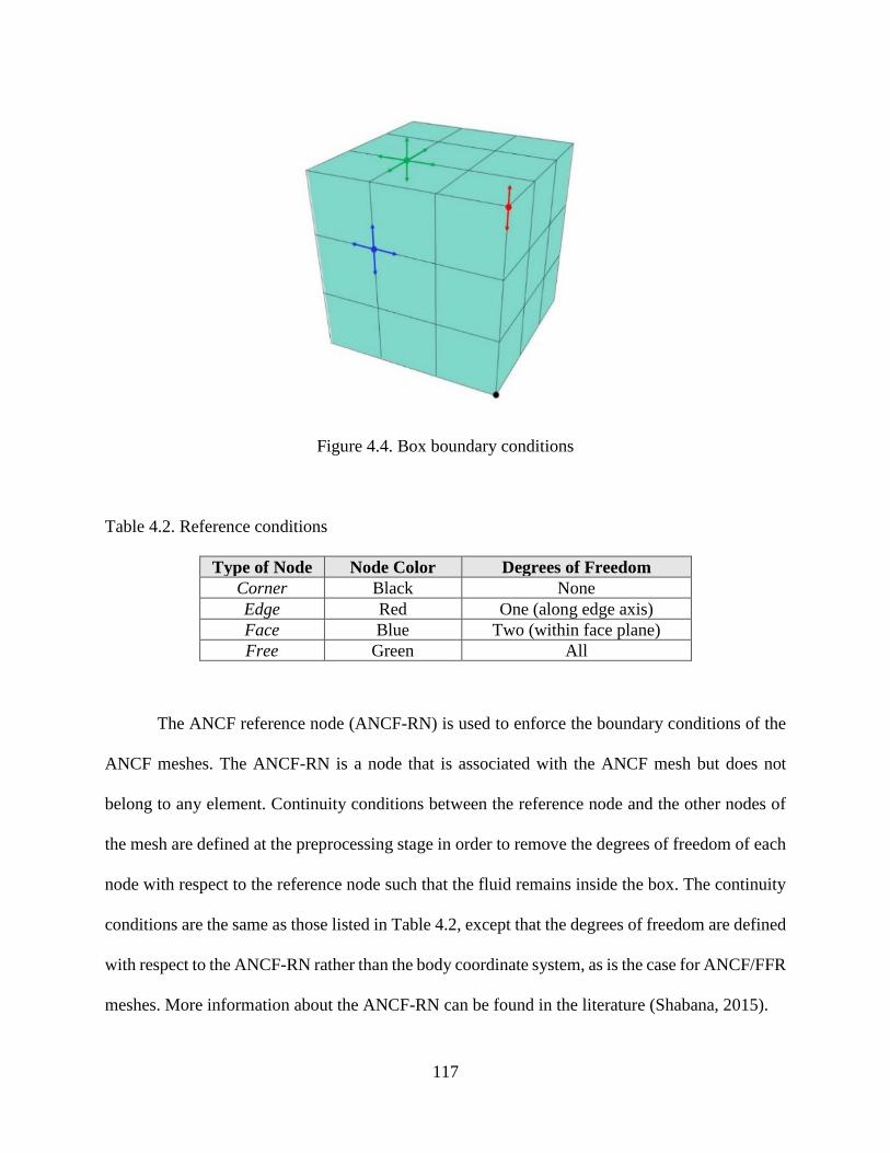
117
Figure 4.4. Box boundary conditions
Table 4.2. Reference conditions
Type of Node Node Color Degrees of Freedom
Corner Black None
Edge Red One (along edge axis)
Face Blue Two (within face plane)
Free Green All
The ANCF reference node (ANCF-RN) is used to enforce the boundary conditions of the
ANCF meshes. The ANCF-RN is a node that is associated with the ANCF mesh but does not
belong to any element. Continuity conditions between the reference node and the other nodes of
the mesh are defined at the preprocessing stage in order to remove the degrees of freedom of each
node with respect to the reference node such that the fluid remains inside the box. The continuity
conditions are the same as those listed in Table 4.2, except that the degrees of freedom are defined
with respect to the ANCF-RN rather than the body coordinate system, as is the case for ANCF/FFR
meshes. More information about the ANCF-RN can be found in the literature (Shabana, 2015).

118
4.6.1.2. Results
(a) (b)
Figure 4.5. Maximum deformation of converged (a) ANCF and (b) ANCF/FFR fluid meshes
The fluid boxes are subjected to a sinusoidal forcing function ( ) ( )0.1sin 8f t t= in order to
generate significant sloshing motion. Figure 4.5 shows the maximum deformation of the
converged ANCF and ANCF/FFR meshes. The vertical position of one of the corner nodes of each
mesh is plotted in Fig. 4.6. In the case of ANCF elements, convergence is achieved using 27
elements, while 512 elements are required to achieve convergence for the ANCF/FFR meshes.
Although the deformation of the ANCF/FFR meshes is smaller than that of the ANCF meshes, the
sloshing behavior is evident, which indicates that the reduced-order ANCF/FFR models can be
useful in situations where modeling the overall fluid motion is necessary and fast simulation time
is desirable, but accurately capturing the fluid free surface is not required, such as in real-time
vehicle modeling which is common in the automotive industry.

119
(a) (b)
Figure 4.6. Vertical corner node position of (a) ANCF meshes and (b) ANCF/FFR meshes
(ANCF meshes: 1, 8, 27, 64 elements;
ANCF/FFR meshes: 27, 125, 216, 512, 1000 elements)
Figure 4.7 plots the CPU times for each mesh, normalized with respect to the 27-element
ANCF/FFR mesh CPU time, versus the number of elements in the mesh, N. The results in Fig. 4.7
demonstrate that although an increased number of ANCF/FFR elements are required to achieve
convergence compared to the ANCF elements, the CPU time for the converged ANCF/FFR mesh
is three times faster than for the converged ANCF mesh due to the use of modal reduction
techniques. In the next section, the effect of the fluid sloshing on the vehicle dynamics will be
investigated using meshes of initially curved ANCF and ANCF/FFR elements.

120
Figure 4.7. Normalized CPU times for the sloshing box models
( ANCF, ANCF/FFR)
4.6.2. Tanker Truck Model
In this section, a tanker truck model is considered in order to highlight the differences between
ANCF and ANCF/FFR finite elements for the analysis of fluid sloshing effects on overall vehicle
motion. The tank is assumed to be half-filled with water in order to induce the most severe sloshing.
Figure 4.8. Medium-duty tanker truck MBS model

121
The vehicle considered in this investigation is the medium-duty tanker truck, pictured in
Fig. 4.8, which was described in Chapter 2. The model includes 20 rigid bodies with 32 degrees
of freedom, in addition to the fluid body. The rigid bodies include 10 tires, a four-bar Ackermann
steering mechanism, two rear axles, the frame, a cab, a tank, and a ground body. The tires, which
are modeled using Pacejka’s brush tire model (Pacejka, 2006), are connected to the axles using
revolute joints, and the cab, tank, and frame are rigidly attached. The sprung mass is supported by
a suspension system of 18 spring-damper elements which provide restoring forces in the
longitudinal, lateral, and vertical directions. The wheelbase is 4.064m, the track width is 1.939m,
and the total vehicle weight is 111.67kN. The volume of the tank is roughly 3,000 gallons, typical
of medium-duty trucks which service residential areas.
Figure 4.9. Lane change path
The tanker truck model performs a lane change over a standard-width U.S. highway lane
of 3.7m, as seen in Fig. 4.9. The lane change is negotiated in a short time of 4s in order to induce

122
noticeable lateral sloshing motion. The ANCF fluid is meshed using 48 elements with 1260
degrees of freedom, and the ANCF/FFR fluid is meshed using 112 elements with 1350 degrees of
freedom. Further mesh refinement was shown not to have a significant effect on the solution. The
solution is also obtained for a model in which the fluid is represented by a rigid body fixed to the
inside of the tank in order to isolate the effect of the fluid sloshing on the vehicle motion.
Figure 4.10. Lateral position of fluid center of mass with respect to tank during lane change
maneuver
( ANCF, ANCF/FFR)
Figure 4.10 shows the lateral position of the center of mass of the fluid with respect to the
tank center for the two flexible fluid models. While the first peak agrees well between the two
models, the later peaks of the ANCF/FFR model are elevated compared to the ANCF model. This
is due to the reduced deformation of the fluid, demonstrated in the sloshing box example. Because
the deformation of the ANCF/FFR is less than the ANCF fluid, the magnitude of the viscous forces
is smaller, resulting in reduced energy dissipation and increased sloshing amplitudes. However,

123
while the motion is not identical between the ANCF and ANCF/FFR meshes, the peak
displacements achieved during the lane change maneuver are similar, leading to similar effects on
the vehicle dynamics. This is evident in Fig. 4.11, which shows the normal forces, and Fig. 4.12,
which shows the lateral friction forces on a left-hand and right-hand tire of the three vehicle models.
The sloshing forces exerted by the flexible fluid on the tank propagate through the suspension to
the tires, resulting in oscillations in the contact forces. The peak magnitudes of the forces exerted
on the tires during the lane change maneuver match very closely. The rigid fluid model, however,
underpredicts the peak contact forces due to the absence of the sloshing, and no oscillation in the
forces occurs after the lane change is complete because the fluid is fixed to the tank.
(a) (b)
Figure 4.11. (a) Normal force on (a) a left-hand tire and (b) a right-hand tire during a lane change
( ANCF, ANCF/FFR, Rigid)

124
Figure 4.12. Lateral friction force on (a) a left-hand tire and (b) a right-hand tire during lane
change ( ANCF, ANCF/FFR, Rigid)
Table 4.3 lists the CPU times normalized with respect to the rigid fluid simulation CPU
time. The ANCF model simulation required over 5.5 times as long to run compared to the
ANCF/FFR model, highlighting the efficiency of the reduced-order ANCF/FFR fluid model
compared to the higher order ANCF model. It is clear from these results that although the reduced-
order ANCF/FFR fluid model does not capture the fluid deformation as accurately as the high-
order ANCF fluid mesh, the overall vehicle motion closely resembles that of the vehicle model
with ANCF fluid but at a reduced computational expense, demonstrating that the new ANCF/FFR
elements can effectively be used to model fluid sloshing in vehicle applications.
Table 4.3. Normalized vehicle model CPU times
Fluid Model Type Normalized CPU Time
Rigid 1
ANCF/FFR 785.9
ANCF 4,325.5

125
4.7. Concluding Remarks
Reduced-order models are often used in MBS and structural applications, however finite element
meshes using conventional elements with infinitesimal rotations as nodal coordinates do not
correctly capture the geometry in the reference configuration. For this reason, the geometrically-
exact ANCF/FFR elements were recently proposed in order to address this fundamental modeling
problem. In this chapter, the ANCF/FFR solid elements are integrated for the first time with a fully
nonlinear MBS vehicle algorithm. ANCF/FFR elements are able to capture initially curved
structures, such as the fluid within a cylindrical tank, while retaining the same number of degrees
of freedom as conventional elements and taking advantage of modal reduction techniques,
resulting in faster simulation times compared to the higher-order ANCF elements. In this chapter,
the solid element is developed in terms of constant geometric coefficients which are obtained using
the matrix of position vector gradients defined in the reference configuration. ANCF elements are
used as the basis for developing the ANCF/FFR elements, which are therefore related to B-splines
and NURBS by a linear mapping, and thus no geometry distortion occurs when CAD models are
converted to FE meshes. The procedure for writing the ANCF gradient vector coordinates in terms
of the FFR nodal rotations is described, which allows for effectively separating the initial geometry
from the displacement coordinates. Using this procedure, the new displacement shape function
matrix, which accounts for the initially curved structure, can be developed. The fluid constitutive
model, which is based on the Navier-Stokes fluid model, is detailed and the incompressibility
conditions, which are enforced using a penalty approach, are defined. The boundary conditions
between the fluid and tank, also enforced using a penalty approach, are detailed. Both normal and
tangential contact forces are included in this chapter. A model of a box filled with fluid which is
subjected to sinusoidal forcing is considered and the components of the MBS vehicle model

126
considered in this chapter, a medium-duty tanker truck with tank half filled with water, are
described. The fluid in both cases is meshed using ANCF and ANCF/FFR elements, and an
equivalent vehicle model in which the fluid is represented by a rigid body is also developed in
order to shed light on the effect of fluid sloshing on the vehicle dynamics when the different finite
element formulations are used.
The sloshing box model demonstrates that while the sloshing amplitudes of the ANCF/FFR
meshes are reduced compared to the converged ANCF fluid meshes, the general sloshing behavior
is still captured and at a significantly reduced CPU time, indicating that the elements may be useful
in certain applications such as vehicle dynamics where the capturing the exact shape of the free
surface is not critical and rapid simulation time is advantageous. This conclusion was confirmed
by the results of the highway vehicle lane change simulation – the sloshing amplitudes of the center
of mass predicted using the ANCF/FFR fluid mesh are found to be in a good agreement with what
predicted by the ANCF mesh. Furthermore, the results of the overall vehicle-dynamics, as
measured by the tire contact forces predicted using the two different meshes, are found to be in a
good agreement. Therefore, it is shown that if the goal is to accurately capture the free-surface
displacement of the fluid, then ANCF elements are better candidates due to their high order and
ability to capture complex shapes. However, if the goal is to perform efficient simulations in order
to obtain the overall vehicle motion, then using ANCF/FFR elements are a better alternative.

127
CHAPTER 5
SUMMARY AND CONCLUSIONS
In Chapter 2, a total Lagrangian ANCF fluid formulation that can be systematically integrated with
fully nonlinear MBS vehicle algorithms is proposed. The new approach can capture the fluid
distributed inertia and viscosity, can accurately predict the change in inertia due to the change in
shape of the fluid, and can visualize the change in the fluid free surface, unlike other discrete inertia
models which do not capture these significant details. The outward forces on the fluid during curve
negotiation are derived and it is shown that these forces do not take the same simple form as the
case of a rigid body negotiating a curve. As discussed in this chapter, accurate modeling of the
fluid geometry using ANCF elements can be achieved without the need for using computational
geometry methods such as B-spline and NURBS representations which have a rigid recurrence
structure unsuitable for MBS analysis. By using the approach proposed in this chapter, one
geometry/analysis mesh is used from the outset. The fluid constitutive law and the fluid/tank
interaction forces are developed. The penalty method is used to ensure that the fluid remains within
the boundaries defined by the tank geometry. Both normal and tangential penalty contact forces
are considered in this study. The MBS vehicle model components are described and the dynamics
of the vehicle is examined using three contrasting motion scenarios in order to study the effect of
sloshing on vehicle dynamics. The braking scenario examines the case of longitudinal sloshing of
the fluid, a rapid lane change produces alternating lateral fluid forces on the tank, and curve
negotiation sheds light on the case of steady-state outward forces due to the centrifugal effect.
The results presented in this chapter demonstrate that depending on the scenario, the
sloshing phenomenon can increase the contact forces on some wheels while decreasing contact

128
forces on other wheels, and this can lead to vehicle instability. In the case of brake applications,
the fluid in the partially-filled tank surges forward, causing uneven wheel loading; in cases of
severe braking, wheel lift may occur on the rear wheels of the vehicle. This can lead to difficulty
controlling the vehicle and increased stopping distances due to lessened road contact, and the
decrease in stability may result in jack-knifing for tractor-trailer vehicles. When entering a curve
or performing a lane change, the outward centrifugal forces cause lateral displacement of the fluid,
which also causes uneven wheel loading. In extreme cases of high speed or small radius of
curvature, these changes could be significant enough to induce wheel lift on the inner wheels and
increase the possibility of rollover compared to an equivalent truck carrying rigid materials.
Furthermore, in cases where tire friction forces are decreased, such as on wet or icy roads, the
possibility for vehicle instability increases even further and drivers must exercise extra caution.
Future analysis can result in defining general rules for speed reduction of a tanker truck entering a
curve in order to maximize vehicle stability and driver safety, proposing modifications to the tank
geometry to reduce sloshing amplitudes and forces, studying the effect of viscosity and
incompressibility on the fluid dynamic behavior, and comparison with conventional finite
elements as well as the smoothed particle hydrodynamics (SPH) method (Wasfy et al., 2014).
In Chapter 3, the newly proposed approach for the integration of a continuum-based
sloshing model with vehicle models is presented using a fully nonlinear MBS rail vehicle model.
The contributions of this chapter are as follows: (1) A unified geometry/analysis mesh is used from
the outset in order to accurately capture complex fluid and rail tank-car geometries as well as the
nonlinear dynamic behavior of the fluid and vehicle. The approach developed in this chapter is
used to examine the effects of liquid sloshing on railroad vehicle dynamics when negotiating a
curve and during traction or braking; (2) The method of the tank-car and fluid geometry description
129
is introduced and it is shown how a unified geometry/analysis mesh can be developed for both the
rigid rail and continuum fluid bodies. The search method used to define the fluid/tank contact
points is outlined and the penalty force model used to describe the fluid/tank interaction forces is
formulated; (3) The fluid constitutive equations that account for the viscosity and incompressibility
effects are presented. The liquid sloshing model developed in this chapter is integrated with the
MBS railroad vehicle model which takes into consideration the nonlinear three-dimensional
wheel/rail contact forces and the wheel and rail profile geometries; and (4) In order to
systematically examine the effect of the motion of the flexible fluid on vehicle dynamics when the
vehicle is negotiating a curve, a general definition of the outward inertia force of a flexible body
using both FFR and ANCF descriptions is investigated. The analysis presented in this chapter
shows that this force depends strongly on the motion of the continuum and does not take the simple
form used in the case of rigid body dynamics.
Comparative simulations were performed to examine the liquid sloshing effects by using
flexible and rigid body fluid models. It is shown that the liquid sloshing can exacerbate the
unbalanced effects when the vehicle travels at a velocity away from the balance speed, but this
effect decreases when the forward velocity is close to the balance speed because the liquid
experiences the same centrifugal force as the rigid fluid body in this case. The results in the traction
analysis show that the liquid motion can significantly affect the load distribution between the front
and rear trucks. Comparing with the ECP braking case, there is a larger coupler force when the
conventional braking is used for both the flexible and rigid body fluid models. Nonetheless, the
results obtained for the model considered in this chapter demonstrate that the liquid sloshing
amplifies the coupler force greatly in the ECP braking case compared to the equivalent rigid body
model because the latter model cannot capture the fluid nonlinear inertia effects.

130
In Chapter 4, the ANCF/FFR elements are integrated for the first time with a fully nonlinear
MBS vehicle algorithm. ANCF/FFR elements are able to capture initially curved structures, such
as the fluid within a cylindrical tank, while retaining the same number of degrees of freedom as
conventional elements and taking advantage of modal reduction techniques, resulting in faster
simulation times compared to the higher-order ANCF elements. In this paper, the solid element is
developed in terms of constant geometric coefficients which are obtained using the matrix of
position vector gradients defined in the reference configuration. ANCF elements are used as the
basis for developing the ANCF/FFR elements, which are therefore related to B-splines and
NURBS by a linear mapping, and thus no geometry distortion occurs when CAD models are
converted to FE meshes. The procedure for writing the ANCF gradient vector coordinates in terms
of the FFR nodal rotations is described, which allows for effectively separating the initial geometry
from the displacement coordinates. Using this procedure, the new displacement shape function
matrix, which accounts for the initially curved structure, can be developed. The fluid constitutive
model, which is based on the Navier-Stokes fluid model, is detailed and the incompressibility
conditions, which are enforced using a penalty approach, are defined. The boundary conditions
between the fluid and tank, also enforced using a penalty approach, are detailed. Both normal and
tangential contact forces are included in this study. A model of a box filled with fluid which is
subjected to sinusoidal forcing is considered and the components of the MBS vehicle model
considered in this investigation, a medium-duty tanker truck with tank half filled with water, are
described. The fluid in both cases is meshed using ANCF and ANCF/FFR elements, and an
equivalent vehicle model in which the fluid is represented by a rigid body is also developed in
order to shed light on the effect of fluid sloshing on the vehicle dynamics when the different finite
element formulations are used.

131
The sloshing box model demonstrates that while the sloshing amplitudes of the ANCF/FFR
meshes are reduced compared to the converged ANCF fluid meshes, the general sloshing behavior
is still captured and at a significantly reduced CPU time, indicating that the elements may be useful
in certain applications such as vehicle dynamics where the capturing the exact shape of the free
surface is not critical and rapid simulation time is advantageous. This conclusion was confirmed
by the results of the highway vehicle lane change simulation – the sloshing amplitudes of the center
of mass predicted using the ANCF/FFR fluid mesh are found to be in a good agreement with what
predicted by the ANCF mesh. Furthermore, the results of the overall vehicle-dynamics, as
measured by the tire contact forces predicted using the two different meshes, are found to be in a
good agreement. Therefore, it is shown that if the goal is to accurately capture the free-surface
displacement of the fluid, then ANCF elements are better candidates due to their high order and
ability to capture complex shapes. However, if the goal is to perform efficient simulations in order
to obtain the overall vehicle motion, then using ANCF/FFR elements are a better alternative.

132
APPENDIX A
Permission for use of author’s previously published Journal of Sound and Vibration article in this
thesis.

133

134
APPENDIX B
Permission for use of author’s previously published Journal of Multi-Body Dynamics article in
this thesis.

135

136
APPENDIX C
The three-dimensional ANCF solid element, with an incomplete polynomial representation, used
in this investigation is an 8-node element. The nodal coordinates jk
e at the node k of the finite
element j can be defined as
T T T T T
1, ,8jk jk jk jk jk
x y z k = =
e r r r r (C. 1)
where jk
r is the absolute position vector at the node k of the element j , and jk
xr , jk
yr and jk
zr are
the position vector gradients obtained by differentiation with respect to the spatial coordinates ,x y
and z , respectively. The displacement field of each coordinate of the solid fluid element can be
defined using an incomplete polynomial with 32 coefficients as
( ) 2 2 2
1 2 3 4 5 6 7 8 9 10
3
3 3 3 2 2 2 2 2 2
11 12 13 14 15 16 17 18 19
3 3 3 3 3 3 2
20 21 22 23 24 25 26 27
2 2
28 29 30 31
3
, ,x y z x y z x y z xy yz xz
x y z x y x z y z xy xz yz
xyz x y x z xy y z x
x
z yz x yz
xy z xy yzz xy
= + + + + + + + + +
+ + + + + + + + +
+ + + + + + + +
+ ++ + 3
32z xyz+
(C. 2)
In this equation, , 1, 2, ,32k k = , are the polynomial coefficients. Using this polynomial
description, the shape functions of the ANCF brick fluid element can be derived as follows:
( ) ( )( )( )
( )( ) ( )( ) ( )( )( )
( ) ( ) ( ) ( )
( ) ( ) ( ) ( )
( ) ( ) ( ) ( )
1,1
2 1 11,2
1 2 1,3
1 1 21,4
1
1 1 1 1
1 1 2 1 2 1 2
1 1 1 1
1 1 1 1
1 1 1 1
k
k
k
k k k
k k k k kk k
k k k k kk k
k k k k kk k
k
k k k
k k k
k
k
k
S
S a
S b
S c
+ + +
+ − −
+
−+
+ − − −
+ − − −+
= − + − + − + −
+
− − + − − + − −
= − − − −
= − − − −
= − − − −
1,2, ,8k
=
(C. 3)
where ,a b , and c are, respectively, the dimensions of the element along the axes ,x y , and z
directions, / , / , /x a y b z c = = = , , , 0,1 , and , ,k k k are the dimensionless

137
nodal locations for node k . The position vector of an arbitrary material point on element j can be
written as
8,1 ,2 ,3 ,4
1
j k k k k jk j j
k
S S S S=
= = r I I I I e S e (C. 4)
where I is the 3 3 identity matrix, j
S and j
e are, respectively, the element shape function
matrix and the vector of nodal coordinates which can be written as
T T T T T T T T
1,1 1,2 1,3 1,4 8,1 8,2 8,3 8,4
1 2 3 4 5 6 7 8
j
Tj j j j j j j j j
S S S S S S S S =
=
S I I I I I I I I
e e e e e e e e e (C. 5)

138
REFERENCES
1. Aboubakr, A.K., Volpi, M., and Shabana, A.A., 2015, “Efficient and robust implementation of
the TLISMNI method”. Journal of Sound and Vibration, 353, pp. 220-242.
2. Aboubakr, A.K., Volpi, M., Shabana, A.A., Cheli, F., and Melzi, S., 2016, “Implementation of
electronically controlled pneumatic brake formulation in longitudinal train dynamics
algorithms”. Proceedings of the Institution of Mechanical Engineers, Part K: Journal of Multi-
body Dynamics, online first, DOI: 1464419316628764
3. Abramson, H.N., 1966, “The dynamic behaviour of liquids in moving containers”. NASA SP-
106.
4. Aliabadi, S., Johnson, A., and Abedi, J., 2003, “Comparison of finite element and pendulum
models for simulation of sloshing”. Computers and Fluids, 32, pp. 535-545.
5. ANSYS, 2019, “ANSYS Fluent”. https://www.ansys.com/products/fluids/ansys-fluent
(accessed 6/11/2019).
6. Ashtianti, I.H., Rakheja, S., and Ahmed, A.K.W., 2015, “Hunting and derailment analysis of
a partly-filled railway tank car”, International Heavy Haul Association Conference, Perth,
Western Australia.
7. Atif, M.M., Chi, S.W., Grossi, E., and Shabana, A.A., 2019, “Evaluation of breaking wave
effects in liquid sloshing problems: ANCF/SPH comparative study”, Nonliner Dyn DOI:
10.1007/s11071-019-04927-5.
8. Bolarinwa, E.O., Mahadevaiah, E., Marzougui, D., and Opiela, K.S., 2012, “The development
of an enhanced finite element tire model for roadside safety hardware assessment”. Journal of
Multibody Dynamics, 226, pp. 206-219.
139
9. Boffi, D. and Gastaldi, L., 2016, “Discrete models for fluid-structure interactions: the finite
element immersed boundary method”, Discrete and Continuous Dynamics Systems: Series S
9(1), pp. 89-107, DOI: 10.3934/dcdss.2016.9.89.
10. Bruzelius, F., Hjort, M., and Svendenius, J., 2013, “Validation of a basic combined-slip tyre
for use in friction estimation applications”. Journal of Automobile Engineering, 228, pp. 1622-
1629.
11. Cottrell, J.A., Hughes, T.J.R., and Reali, A., 2007, “Studies of Refinement and Continuity in
the Isogeometric Analysis”, Comput. Methods in Appl. Mech. Engrg., 196, pp. 4160-4183.
12. Chen, G.F., and Wu, C.H., 2011, “Effects of excitation angle and coupled heave–surge–sway
motion on fluid sloshing in a three-dimensional tank”, J. Mar. Sci. Technol 16, pp. 22-50, DOI:
10.1007/s00773-010-0111-0.
13. Cui, D., Yan, S., Guo, X., and Gao, R., 2014, “Parametric resonance of liquid sloshing in
partially filled spacecraft tanks during the powered-flight phase of rocket”. Aerospace Science
and Technology, 35, pp. 93-105.
14. Cundall, P.A. and Strack, O.D.L., 1979, “A discrete numerical model for granular assemblies”,
Geotechnique 29(1), pp. 47-65.
15. De-Juan, A., Sancibrian, R., and Viadero, F., 2012, “Optimal synthesis of function generation
in steering linkages”. International Journal of Automotive Technology, 13, pp. 1033-146.
16. Di Gialleonardo, E., Premoli, A., Gallazi, S., and Bruni S., 2013, “Sloshing effects and running
safety in railway freight vehicles”, Vehicle System Dynamics 51(10), pp. 1640-1654, DOI:
10.1080/00423114.2013.814797.
17. Dodge, 2000, “The new ‘dynamic behavior of liquids in moving containers’”, Southwest
Research Institute, San Antonio, Texas.

140
18. Gialleonardo, E.D., Premoli, A., Gallazi, S., and Bruni S., 2013, “Sloshing effects and running
safety in railway freight vehicles”, Vehicle System Dynamics 51(10), pp. 1640-1654, DOI:
10.1080/00423114.2013.814797.
19. Godderidge, B., Turnock, S., and Mingyi, T., 2011, “A rapid method for the simulation of
sloshing using a mathematical model based on the pendulum equation”, Computers & Fluids
57, pp. 163-171.
20. Graham, E.W., 1951, “The forces produced by fuel oscillations in a rectangular tank”. Douglas
Aircraft Cooperation, SM-13748.
21. Graham, E.W. and Rodríguez, A.M., 1952, “The characteristics of fuel motion which affect
airplane dynamics”. Journal of Applied Mechanics, 74, pp. 381-388.
22. Griffiths, W.D. and Boysan, F., 1996, “Computational Fluid dynamics (CFD) and empirical
modelling of the performance of a number of cyclone samplers”, J. Aerosol Sci. 27(2), pp. 281-
304.
23. Grossi, E. and Shabana, A.A., 2017, “Validation of a total lagrangian ANCF solution
procedure for fluid-structure interaction problems”, J. Verif. Valid. Uncertain. Quantif. 2(4),
041001-1-041001-13.
24. Grossi, E. and Shabana, A.A., 2018, “ANCF analysis of the crude oil sloshing in railroad
vehicle systems”, Journal of Sound and Vibration 433, pp. 493-516.
25. Ibrahim, R.A., 2005, Liquid Sloshing Dynamics: Theory and Applications, Cambridge
University Press.
26. Ibrahim, R.A., Pilipchuk, V.N., and Ikeda, T., 2001, “Recent advances in liquid sloshing
dynamics”. Applied Mechanics Reviews, 54, pp. 133-199.

141
27. Kalker, J.J., 1990, Three-Dimensional Elastic Bodies in Rolling Contact, Kluwer Academic
Publishers, Dordrecht, The Netherlands.
28. King, C. and Trichur, R., 2015, “Train carrying crude oil derails in Ontario”. WSJ,
http://www.wsj.com/articles/train-carrying-crude-oil-derails-in-ontario-1424015961.
29. Liu, M.B. and Liu, G.R., 2010, “Smoothed particle hydrodynamics (SPH): an overview and
recent developments”. Archives of Computational Methods in Engineering, 17, pp. 25-76.
30. Mackenzie, D., 2012, “Curing ill surfaces”, SIAM News, 6 April 2011.
31. Monaghan, J.J., 2012, “Smoothed particle hydrodynamics and its diverse applications”, Annu.
Rev. Fluid Mech. 44, pp. 323-46, DOI: 10.1146/annurev-fluid-120710-101220.
32. Nichkawde, C., Harish, P.M, and Ananthkrishnan, N., 2004, “Stability analysis of a multibody
system model for coupled slosh-vehicle dynamics”. Journal of Sound and Vibration, 275, pp.
1069-1083.
33. Nicolsen, B., Wang, L., and Shabana, A.A., 2017, “Nonlinear finite element analysis of liquid
sloshing in complex vehicle motion scenarios”. Journal of Sound and Vibration, 405, pp. 208-
233.
34. Nishiura, D. and Sakagushi, H., 2014, “Wet dispersion mechanism of fine aggregates in
multiphase flow with solid beads under simple shear”, AIChE Journal 60(12), pp. 4076-4085.
35. Olshevskiy, A., Dmitrochenko, O., and Kim, C.W., 2013, “Three-dimensional solid brick
element using slopes in the absolute nodal coordinate formulation”. ASME Journal of
Computational and Nonlinear Dynamics, 9, doi:10.1115/1.4024910
36. Pacejka, H.B.,2006, Tyre and Vehicle Dynamics, Elsevier, Oxford, England, Second Edition.

142
37. Pape, D., Thornton, B., and Yugulis, K., 2016, “Slosh characteristics of aggregated
intermediate bulk containers on single-unit trucks”. Federal Motor Carrier Safety
Administration, U.S. Department of Transportation, Washington, D.C.
38. Patel, M., Orzechowski, G., Tian, Q., and Shabana, A.A., 2016, “A new multibody system
approach for tire modeling using ANCF finite elements”. Proceedings of the Institution of
Mechanical Engineers, Part K: Journal of Multi-body Dynamics, 230, pp. 69-84.
39. Pelc, J., 2007, “Towards realistic simulation of deformations and stresses in pneumatic tyres”.
Applied Mathematical Modelling, 31, pp. 530-540.
40. Petravic, J., 2007, “On the equilibrium calculation of the friction coefficient for liquid slip
against a wall,” Journal of Chemical Physics, Vol. 127.
41. Piegl, L. and Tiller, W., 1997, The NURBS Book, Second Edition, Springer, New York.
42. Pit, R., Hervet H., and Leger, L., 1999, “Friction and slip of a simple liquid at a solid surface,”
Tribology Letters, pp. 147-152.
43. Ranganathan, R., Rakheja, S., and Sankar, S., 1989, “Steady turning stability of partially filled
tank vehicles with arbitrary tank geometry”. Journal of Dynamic Systems, Measurement, and
Control, 111, pp. 481–489.
44. Sanborn, G., Tobaa, M. and Shabana, A.A., 2008, “Coupling between structural deformations
and wheel-rail contact geometry in railroad vehicle dynamics”. Proceedings of the Institution
of Mechanical Engineers, Part K: Journal of Multi-body Dynamics, 222(4), p.381-392.
45. Shabana, A.A., 2013, Dynamics of Multibody Systems, Cambridge University Press, Oxford,
England, Fourth Edition.
46. Shabana, A.A., 2015, “ANCF tire assembly model for multibody system applications”.
Journal of Computational and Nonlinear Dynamics, 10, ID 024504.

143
47. Shabana, A.A., 2017A, Computational Continuum Mechanics, Cambridge University,
Cambridge, UK, Third edition.
48. Shabana, A.A., 2017B, “Geometrically accurate floating frame of reference finite elements for
the small deformation problem”, Proc. Inst. Mech. Eng. Part K: J. Multibody Dyn. 232(2), pp.
286–292.
49. Shabana, A.A., 2018, “Geometrically accurate infinitesimal-rotation spatial finite elements”,
Proc. Inst. Mech. Eng. Part K: J. Multibody Dyn. 233(1) pp. 182-187, DOI:
10.1177/1464419318774948.
50. Shabana, A.A., Tobaa, M., Sugiyama, H. and Zaazaa, K., 2005. “On the Computer
Formulations of the Wheel/Rail Contact Problem”. Nonlinear Dynamics, 40(2), p.169-193.
51. Shabana, A.A., Wang, G., and Kulkarni, S., 2018, “Further investigation on the coupling
between the reference and elastic displacements in flexible body dynamics”, Journal of Sound
and Vibration 427, pp. 159–777, DOI: 10.1016/j.jsv.2018.02.054.
52. Shabana, A.A., Zaazaa, K.E., and Sugiyama, H., 2008, Railroad Vehicle Dynamics: A
Computational Approach, Taylor & Francis/CRC, Boca Raton, FL.
53. Shen, X., Yan, Y., Li, X., Xie, C., Wang, L., 2014, “Analysis on tank truck accidents involved
in road hazardous materials transportation in China”. Traffic Injury Prevention, 15, pp. 762-
768.
54. Shi, H., Wang, L., Nicolsen, B., Shabana, A.A., 2017, “Integration of geometry and analysis
for the study of liquid sloshing in railroad vehicle dynamics”. Proceedings of the Institution of
Mechanical Engineers, Part K: Journal of Multi-body Dynamics, 231(4), pp. 608-629.
55. Spencer, A.J.M., 1980, Continuum Mechanics, Longman, London, England.

144
56. Sugiyama, H., and Shabana, A., A., 2007, “Trajectory Coordinate Constraints in Multibody
Railroad Vehicle Systems”, Journal of System Design and Dynamics 1(3), DOI:
10.1299/jsdd.1.481.
57. Tinsley, B. and Shabana, A.A., 2019, “Eigenvalue convergence of the geometrically accurate
spatial beam, plate, and solid elements”, Technical Report # MBS2019-1-UIC.
58. U.S. Department of Transportation, Federal Motor Carrier Safety Administration, 2007,
“Cargo tank rollover myths and truths”. https://www.fmcsa.dot.gov/sites/fmcsa.dot.gov/files/
docs/FINAL_Cargo_Tank_Rollover_Fact_Sheet_508.pdf (accessed 2.16.17).
59. U.S. Department of Transportation, Federal Highway Administration, 2011, “Freight facts and
figures”. http://www.ops.fhwa.dot.gov/freight/freight_analysis/nat_freight_stats/docs/
11factsfigures/pdfs/fff2011_highres.pdf (accessed 2.16.17).
60. U.S. Department of Transportation, Pipeline and Hazardous Materials Safety Administration,
2011, “Hazardous Materials Incident Report”, Incident ID E-2011080424. Accessed 5/31/2019
(https://portal.phmsa.dot.gov/xmlpserver/loading.jsp?_xdo=%2FEIA+Forms%2
F5800Incident.xdo&_id=1410e6fe-d686-4593-b73c-7176221c2c83&_genstatus=).
61. U.S. Department of Transportation, National Highway and Traffic Safety Administration,
2015, “Electronic stability control systems for heavy vehicles”. https://www.transportation.
gov/sites/dot.gov/files/docs/FMVSS-136-Final-Rule-05182015-final.pdf (accessed 2/16/17).
62. U.S. Department of Transportation, Pipeline and Hazardous Materials Safety Administration,
2015, “10 year incident summary reports”. https://hip.phmsa.dot.gov/analyticsSOAP/saw.dll?
Dashboard&NQUser=HazmatWebsiteUser1&NQPassword=HazmatWebsiteUser1&PortalPa
th=/shared/Public%20Website%20Pages/_portal/10%20Year%20Incident%20Summary%20
Reports (accessed 2.16.17).

145
63. Vera, C., Paulin, J., Suarez, B., and Gutiérrez, M., 2005, “Simulation of freight trains equipped
with partially filled tank containers and related resonance phenomenon”. Proceedings of the
Institution of Mechanical Engineers, Part F: Journal of Rail and Rapid Transit, 219(4), pp.
245-259.
64. Wang, L., Jimenez-Octavio, J.R., Wei, C., and Shabana, A.A., 2014, “Low Order Continuum-
Based Liquid Sloshing Formulation for Vehicle System Dynamics”, Journal of Computational
and Nonlinear Dynamics, 10(2), ID 021022.
65. Wang, L., Jimenez-Octavio, J.R., Wei, C., and Shabana, A.A., 2015, “Low order continuum-
based liquid sloshing formulation for vehicle system dynamics”. Journal of Computational
and Nonlinear Dynamics, 10, ID 021022.
66. Wang, L., Shi, H. and Shabana, A.A., 2016, “Effect of the tank-car thickness on the nonlinear
dynamics of railroad vehicles”. Proceedings of the Institution of Mechanical Engineers, Part
K: Journal of Multi-body Dynamics, DOI: 10.1177/1464419316642930.
67. Wasfy, T.M., Wasfy, H.M., and Peters, J.M., 2014, “Coupled multibody dynamics and
smoothed particle hydrodynamics for predicting liquid sloshing for tanker trucks”, ASME
DETC2014-35191, Proceedings of the ASME 2014 International Design Engineering
Technical Conferences & Computers and Information in Engineering Conference, Buffalo,
New York.
68. Wei, C., Wang, L., and Shabana, A.A., 2015, “A total Lagrangian ANCF liquid sloshing
approach for multibody system applications”. Journal of Computational and Nonlinear
Dynamics, 10(5), ID 051014.
69. White, F.M., Fluid Mechanics, 2011, The McGraw-Hill Companies, Inc., New York, Seventh
edition.

146
70. Wronski, R., 2013, “As more oil flows by rail, concerns grow about safety of the tank-cars”.
tribunedigital-chicagotribune, http://articles.chicagotribune.com/2013-11-29/news/ct-
dangerous-tank-cars-met-1129-20131129_1_tank-cars-oil-production-more-oil-flows.
71. WSB-TV Atlanta, Driver dies in fiery tanker crash on I-985 in Hall County,
http://www.wsbtv.com/news/local/tanker-truck-fire-shuts-down-i-985-hall-county/17241607,
2015 (accessed 2.16.17).
72. Xue-Lian, Z., Xian-Sheng, L., and Yuan-Yuan, R., 2012, “Equivalent mechanical model for
lateral liquid sloshing in partially filled tank vehicles”, Mathematical Problems in Engineering,
Article ID: 162825, DOI: 10.1155/2012/162825.
73. Yang, S.H., Lee, S.B., Park, J.H., Han, S.Y., Choi, Y.M., DO, J., Kwon, S.H., and Molin, B.,
2016, “Experimental study on piston- and sloshing-mode moonpool resonances”, J. Mar. Sci.
Technol. 21, pp. 715-728, DOI: 10.1007/s00773-016-0386-x.
74. Zhang, Z., Wang, T., and Shabana, A.A., 2019, “Development and implementation of
geometrically accurate reduced-order models: Convergence properties of planar beams”,
Journal of Sound and Vibration 439, pp. 457–478, DOI: 10.1016/j.jsv.2018.06.005.
75. Zheng, X., Li, X., and Ren, Y., 2012, “Equivalent mechanical model for lateral liquid sloshing
in partially filled tank vehicles”. Mathematical Problems in Engineering, ID 162825.
147
VITA
Brynne Elizabeth Nicolsen
EDUCATION
University of Illinois at Chicago (UIC)
• Ph.D. in Mechanical Engineering; Advisor: Prof. Ahmed A. Shabana || Aug. 2015 – July 2019
GPA: 4.0/4.0
• B.S. in Bioengineering, Minor in Mechanical Engineering || Aug. 2011 – May 2015
GPA: 4.0/4.0, Summa Cum Laude
RELEVANT COURSEWORK
Finite Element Analysis I and II – Nonlinear Finite Element Analysis – Dynamics of Mechanical Systems –
Computer-Aided Analysis of Multibody Systems – Vibration of Discrete and Continuous Systems –
Continuum Mechanics – Theory of Elasticity – Plasticity – Numerical Analysis – Mathematical Theory of Finite
Elements – Mathematical Methods for Engineers
SKILLS
Software: Experienced: SIGMA/SAMS, ANSYS, PTC Creo, Matlab, Fortran || Familiar: MSC Adams,
HyperMesh, NX, TeamCenter
Communication: Exemplary written and oral communication
Interpersonal: Strong leadership qualities, skilled at instruction, collaborates well in groups
RESEARCH EXPERIENCE
Graduate
Dynamic Simulation Laboratory || UIC || June 2015 – July 2019
Comparison of Small- and Large-Deformation Finite Elements for the Study of Fluid Sloshing || Jan. 2016 –
July 2019
• Developed general contact algorithm applicable to rigid or flexible bodies of different finite element types
• Compared fluid sloshing behavior using different finite element formulations in highway vehicle system
applications
Fluid Sloshing Phenomena using Large-Deformation Finite Elements || June 2015 – Dec. 2016
• Developed medium-duty tanker truck model with fluid represented by ANCF continuum finite elements
• Ran model under different scenarios to investigate the effects of fluid-tank interaction on vehicle
dynamics and stability
Undergraduate
Dynamic Simulation Laboratory || UIC || Oct. 2014 – May 2015
• Implemented DEM (discrete element method) module in the general-purpose flexible MBD software
SIGMA/SAMS
• Modeled tire-soil interaction using the DEM approach and ANCF finite elements
• Developed Fortran subroutines including interparticle contact detection and Verlet numerical integration

148
PUBLICATIONS
• Nicolsen, B., Shi, H., Wang, L., Shabana, A., "Integration of Geometry and Analysis for the Study of Liquid Sloshing in Vehicle System Dynamics," Proceedings of the 2017 ASME International Mechanical Engineering Congress and Exposition, November 3-9, 2017, Tampa, FL, USA.
• Nicolsen, B., Wang, L., and Shabana, A., “Nonlinear Finite Element Analysis of Liquid Sloshing in Complex Vehicle Motion Scenarios,” Journal of Sound and Vibration, Vol. 405, May 2017.
• Shi, H., Wang, L., Nicolsen, B., and Shabana, A.A., “Integration of Geometry and Analysis for the Study
of Liquid Sloshing in Railroad Vehicle Dynamics”, Proc IMechE Part K: J Multibody Dynamics, Online
March 2017.
• Contreras, U., Nicolsen, B., Tian, Q., Recuero, A., Shabana, A., “Integration of ANCF and Discrete
Element Method for Multibody Vehicle Applications,” Proceedings of the ASME 2015 International Design
Engineering Technical Conference & Computers and Information in Engineering Conference, August 2-
5, 2015, Boston, MA, USA.
INTERNSHIP EXPERIENCE
Graduate
Navistar, Inc.: Vehicle Dynamics Engineer || Lisle, IL || May 2016 – Aug. 2016
• Developed 20 steer axle and 34 leaf spring model libraries using newly-enhanced modeling techniques
to increase speed of model development
• Assisted in building state-of-the-art hardware-in-the-loop setup to simulate electronic stability control of
class A tractors in support of FMVSS136 vehicle stability regulations
• Characterized test data of 13 tires from a variety of manufacturers in order to develop more accurate
virtual tire models
• Processed and analyzed vehicle test results for use in model correlation and validation
Undergraduate
Hospira: Systems Test Engineer || Lake Forest, IL || May 2016 – Aug. 2016
• Worked with engineers to write, test, and edit protocols for the testing of infusion pumps for re-
manufacture
TEACHING ASSISTANTSHIPS
Graduate
Introduction to Engineering Design and Graphics || UIC || Jan. 2019 – May 2019
• Co-managed a group of 17 undergraduate TAs in developing coursework material and assisting during
lectures
• Developed new methodologies to improve TA productivity and efficiency
• Led discussions on fair TA compensation and redesigning course content
Professional Development Seminar || UIC || Jan. 2016 – May 2017
• Met with students weekly to aid in developing resumes and cover letters and in securing full-time jobs
• Collaborated with three other TAs to maintain course website, record presentations, and ensure lectures
ran smoothly

149
Introductory Vibration Theory || UIC || Aug. 2015 – May 2016
• Guided students in learning to formulate and solve the differential equations of motion for vibrational
systems
• Assisted professor in preparing and grading assignments, projects, and exams, and maintaining course
website
Undergraduate
Engineering Orientation || UIC || Aug. 2013 – Dec. 2013
• Educated a group of freshman students about the field of bioengineering and the curriculum at UIC
• Assisted students in developing their first resumes and applying to summer internships
PRESENTATIONS
• U.S. National Congress for Theoretical and Applied Mechanics, June 4-9, 2018, Chicago IL
Integration of Geometry and Analysis for the Study of Liquid Sloshing in Complex Vehicle Systems
• ASME International Mechanical Engineering Congress and Exposition, November 3-9, 2017, Tampa, FL
Integration of Geometry and Analysis for the Study of Liquid Sloshing in Vehicle System Dynamics
• Workshop on Computational and Nonlinear Dynamics for Industry, May 27, 2016, Chicago, IL
Liquid Sloshing and the Contact Problem
PROFESSIONAL SERVICE
Journal Reviewer:
• Journal of Multi-Body Dynamics, Feb. 2017 || Vehicle System Dynamics, Sept. 2017 || Journal of Rail
and Rapid Transit, July 2018 || Journal of Sound and Vibration, July 2018 || Journal of Vibration and
Acoustics, Sept. 2018
Conference Reviewer:
• ASME International Gas Turbine Institute Exposition, June 2019 (2 papers)
EXTRACURRICULAR ACTIVITIES
Pi Tau Sigma: Mechanical Engineering Honors Society || Member Oct. 2018 – Present
American Society for Engineering Education || Member Aug. 2018 – Present
Tau Beta Pi: Engineering Honors Society || Recording Secretary Apr. 2014 – May 2015; Member Nov. 2012
– Present
UIC Bioengineering Student Journal: Editor Jan. 2013 – May 2016, Exec. Editor Jan 2014 – May 2014,
Author May 2014