follow-on mission for the hubble space telescopecdhall/courses/aoe4065/oldreports/hubble... ·...
TRANSCRIPT

Follow-on Mission for the Hubble Space Telescope
Daniel Bittner, Andrew Cody,Caitlin Eubank, Curtis Jorgensen,
Thomas Reppert, Jay Shultis,Brett Streetman, and David Ziegler
May 10, 2004
Contents
List of Tables iv
List of Figures vi
List of Symbols vii
Nomenclature ix
1 Introduction and Problem Definition 11.1 History and Background . . . . . . . . . . . . . . . . . . . . . . . . . 11.2 Hubble Systems and Operations . . . . . . . . . . . . . . . . . . . . . 21.3 Problem Definition . . . . . . . . . . . . . . . . . . . . . . . . . . . . 4
1.3.1 Required Disciplines, Societal Sectors and Actors . . . . . . . 41.3.2 Scope . . . . . . . . . . . . . . . . . . . . . . . . . . . . . . . 41.3.3 Needs, Alterables, and Constraints . . . . . . . . . . . . . . . 51.3.4 Relevant Elements . . . . . . . . . . . . . . . . . . . . . . . . 5
1.4 Summary . . . . . . . . . . . . . . . . . . . . . . . . . . . . . . . . . 6
2 Value System Design 72.1 Objectives . . . . . . . . . . . . . . . . . . . . . . . . . . . . . . . . . 72.2 Performance . . . . . . . . . . . . . . . . . . . . . . . . . . . . . . . . 72.3 Cost . . . . . . . . . . . . . . . . . . . . . . . . . . . . . . . . . . . . 92.4 Summary . . . . . . . . . . . . . . . . . . . . . . . . . . . . . . . . . 10
3 System Synthesis 113.1 Orbit Options . . . . . . . . . . . . . . . . . . . . . . . . . . . . . . . 113.2 Attitude Systems . . . . . . . . . . . . . . . . . . . . . . . . . . . . . 133.3 Thermal . . . . . . . . . . . . . . . . . . . . . . . . . . . . . . . . . . 133.4 Power . . . . . . . . . . . . . . . . . . . . . . . . . . . . . . . . . . . 14
3.4.1 Solar Arrays . . . . . . . . . . . . . . . . . . . . . . . . . . . . 153.4.2 Batteries . . . . . . . . . . . . . . . . . . . . . . . . . . . . . . 153.4.3 Power Regulation . . . . . . . . . . . . . . . . . . . . . . . . . 173.4.4 Electrical Bus Voltage Control . . . . . . . . . . . . . . . . . . 18
i

CONTENTS ii
3.5 Propulsion . . . . . . . . . . . . . . . . . . . . . . . . . . . . . . . . . 183.6 Communications . . . . . . . . . . . . . . . . . . . . . . . . . . . . . 203.7 Structures . . . . . . . . . . . . . . . . . . . . . . . . . . . . . . . . . 21
3.7.1 Solar Arrays . . . . . . . . . . . . . . . . . . . . . . . . . . . . 213.7.2 Other Structural Components . . . . . . . . . . . . . . . . . . 21
3.8 Science Missions . . . . . . . . . . . . . . . . . . . . . . . . . . . . . . 223.9 Summary . . . . . . . . . . . . . . . . . . . . . . . . . . . . . . . . . 33
4 System Analysis 344.1 Options for Retrofit Mission . . . . . . . . . . . . . . . . . . . . . . . 34
4.1.1 Option 1 . . . . . . . . . . . . . . . . . . . . . . . . . . . . . . 344.1.2 Option 2 . . . . . . . . . . . . . . . . . . . . . . . . . . . . . . 364.1.3 Option 3 . . . . . . . . . . . . . . . . . . . . . . . . . . . . . . 38
4.2 Summary . . . . . . . . . . . . . . . . . . . . . . . . . . . . . . . . . 39
5 System Optimization 415.1 Orbits and Attitude Dynamics . . . . . . . . . . . . . . . . . . . . . . 41
5.1.1 Earth Escape . . . . . . . . . . . . . . . . . . . . . . . . . . . 415.1.2 Transfer to L5 . . . . . . . . . . . . . . . . . . . . . . . . . . . 425.1.3 Orbit About L5 . . . . . . . . . . . . . . . . . . . . . . . . . . 445.1.4 Overall Mission Specifications . . . . . . . . . . . . . . . . . . 455.1.5 Attitude Control . . . . . . . . . . . . . . . . . . . . . . . . . 46
5.2 Propulsion . . . . . . . . . . . . . . . . . . . . . . . . . . . . . . . . . 475.2.1 Benefits of Using Ion Propulsion . . . . . . . . . . . . . . . . . 475.2.2 Propulsion Analysis . . . . . . . . . . . . . . . . . . . . . . . . 48
5.3 Environment . . . . . . . . . . . . . . . . . . . . . . . . . . . . . . . . 505.3.1 Thermal Shield . . . . . . . . . . . . . . . . . . . . . . . . . . 505.3.2 Solar Arrays . . . . . . . . . . . . . . . . . . . . . . . . . . . . 515.3.3 Interior . . . . . . . . . . . . . . . . . . . . . . . . . . . . . . 525.3.4 Exterior . . . . . . . . . . . . . . . . . . . . . . . . . . . . . . 52
5.4 Power . . . . . . . . . . . . . . . . . . . . . . . . . . . . . . . . . . . 535.5 Communications . . . . . . . . . . . . . . . . . . . . . . . . . . . . . 56
5.5.1 Earth Communications . . . . . . . . . . . . . . . . . . . . . . 575.5.2 Data Rate . . . . . . . . . . . . . . . . . . . . . . . . . . . . . 585.5.3 Retrofit Equipment . . . . . . . . . . . . . . . . . . . . . . . . 585.5.4 HST Computer and Data Storage . . . . . . . . . . . . . . . . 61
5.6 Mission Control . . . . . . . . . . . . . . . . . . . . . . . . . . . . . . 625.6.1 Deep Space Network . . . . . . . . . . . . . . . . . . . . . . . 625.6.2 Hubble Mission Control . . . . . . . . . . . . . . . . . . . . . 635.6.3 Service Mission Time . . . . . . . . . . . . . . . . . . . . . . . 655.6.4 Space Telescope Science Institute . . . . . . . . . . . . . . . . 65
5.7 Structures . . . . . . . . . . . . . . . . . . . . . . . . . . . . . . . . . 65

CONTENTS iii
5.7.1 Structural Evaluation . . . . . . . . . . . . . . . . . . . . . . . 665.7.2 Upgrades . . . . . . . . . . . . . . . . . . . . . . . . . . . . . 675.7.3 Propulsion Module . . . . . . . . . . . . . . . . . . . . . . . . 675.7.4 Calculations . . . . . . . . . . . . . . . . . . . . . . . . . . . . 685.7.5 Shuttle Layout . . . . . . . . . . . . . . . . . . . . . . . . . . 685.7.6 Docking and Separation Process . . . . . . . . . . . . . . . . . 69
5.8 Instruments . . . . . . . . . . . . . . . . . . . . . . . . . . . . . . . . 715.9 Summary . . . . . . . . . . . . . . . . . . . . . . . . . . . . . . . . . 72
6 Final Configuration and Conclusions 746.1 Mission Definition . . . . . . . . . . . . . . . . . . . . . . . . . . . . . 74
6.1.1 Objective . . . . . . . . . . . . . . . . . . . . . . . . . . . . . 746.1.2 Requirements and Constraints . . . . . . . . . . . . . . . . . . 75
6.2 Existing Hubble Components . . . . . . . . . . . . . . . . . . . . . . 756.3 Hubble Retrofit Components . . . . . . . . . . . . . . . . . . . . . . . 766.4 Mission Costs . . . . . . . . . . . . . . . . . . . . . . . . . . . . . . . 776.5 Mission Constraints and Optimization . . . . . . . . . . . . . . . . . 786.6 Overall Design Success . . . . . . . . . . . . . . . . . . . . . . . . . . 796.7 Summary . . . . . . . . . . . . . . . . . . . . . . . . . . . . . . . . . 80
A Orbit Code 82
B Power Code 90
C Propulsion Code 93
D Communications Code 95
List of Tables
1.1 Needs, Alterables, and Constraints . . . . . . . . . . . . . . . . . . . 5
2.1 List of Objectives . . . . . . . . . . . . . . . . . . . . . . . . . . . . . 8
3.1 Solar Cell Types . . . . . . . . . . . . . . . . . . . . . . . . . . . . . 163.2 Secondary Batteries . . . . . . . . . . . . . . . . . . . . . . . . . . . . 173.3 Properties of Common Propellants [31] . . . . . . . . . . . . . . . . . 193.4 Properties for Commonly Used Materials [17] . . . . . . . . . . . . . 22
4.1 Full System Option 1 . . . . . . . . . . . . . . . . . . . . . . . . . . . 354.2 Option 1 Advantages and Disadvantages . . . . . . . . . . . . . . . . 364.3 Full System Option 2 . . . . . . . . . . . . . . . . . . . . . . . . . . . 364.4 Option 2 Advantages and Disadvantages . . . . . . . . . . . . . . . . 374.5 Full System Option 3 . . . . . . . . . . . . . . . . . . . . . . . . . . . 384.6 Option 3 Advantages and Disadvantages . . . . . . . . . . . . . . . . 40
5.1 Material properties and surface temperatures . . . . . . . . . . . . . . 515.2 Shield diameters and thickness . . . . . . . . . . . . . . . . . . . . . . 515.3 Acceptable Frequency Band Ranges . . . . . . . . . . . . . . . . . . . 585.4 Antenna Characteristics for a given Band Frequency . . . . . . . . . . 62
6.1 Cost Component Breakdown . . . . . . . . . . . . . . . . . . . . . . . 81
iv

List of Figures
1.1 Diagram of Hubble’s Parts [21] . . . . . . . . . . . . . . . . . . . . . 21.2 Diagram of Hubble’s Pointing System [21] . . . . . . . . . . . . . . . 3
2.1 Objective Hierarchy Flowchart . . . . . . . . . . . . . . . . . . . . . . 9
3.1 Location of Lagrange Points . . . . . . . . . . . . . . . . . . . . . . . 123.2 Diagram of the Advanced Camera for Surveys [20] . . . . . . . . . . . 233.3 Diagram of the Near Infrared Camera and Multi-Object Spectrometer
[20] . . . . . . . . . . . . . . . . . . . . . . . . . . . . . . . . . . . . . 243.4 Diagram of the Space Telescope Imaging Spectrograph [20] . . . . . . 253.5 Diagram of the Wide Field Camera 3: Schematic on left, CAD con-
ception of WFC3 on right [21] . . . . . . . . . . . . . . . . . . . . . . 263.6 Diagram of the Cosmic Origins Spectrograph [20] . . . . . . . . . . . 283.7 Diagram of the Fine Guidance Sensors [20] . . . . . . . . . . . . . . . 293.8 Orbit of an Aten Asteroid . . . . . . . . . . . . . . . . . . . . . . . . 313.9 Damage on Car from Meteorite [9] . . . . . . . . . . . . . . . . . . . 313.10 The Barringer Crater [9] . . . . . . . . . . . . . . . . . . . . . . . . . 323.11 The Tunguska Event [9] . . . . . . . . . . . . . . . . . . . . . . . . . 33
5.1 HST Earth escape orbit . . . . . . . . . . . . . . . . . . . . . . . . . 435.2 Phasing transfer orbit to L5 . . . . . . . . . . . . . . . . . . . . . . . 445.3 Set up for the restricted three-body problem (modified from Schaub [26]) 455.4 HST orbit relative to L5, in a rotating frame of view . . . . . . . . . 465.5 Current Hubble Thermal Configuration with only MLI . . . . . . . . 535.6 Hubble Configuration with Added OSR to replace MLI . . . . . . . . 545.7 Solar Array sizing. Array area as a function of production efficiency. . 575.8 Eb/No vs Antenna Diameter . . . . . . . . . . . . . . . . . . . . . . . 605.9 Eb/No vs Data Rate . . . . . . . . . . . . . . . . . . . . . . . . . . . 615.10 CAD Model of the Hubble with New Retrofit Components . . . . . . 665.11 Solar Array Configuration . . . . . . . . . . . . . . . . . . . . . . . . 675.12 Propulsion Module . . . . . . . . . . . . . . . . . . . . . . . . . . . . 685.13 Propulsion Module with Flight Support System . . . . . . . . . . . . 695.14 Shuttle Layout . . . . . . . . . . . . . . . . . . . . . . . . . . . . . . 70
v

LIST OF FIGURES vi
5.15 Space Based Visible [16] . . . . . . . . . . . . . . . . . . . . . . . . . 725.16 View of Space Based Visible Camera [16] . . . . . . . . . . . . . . . . 735.17 Space Based Visible Data Filter: The picture on the left is the full-
frame CCD exposure and the right is an associated signal processorimage. [16] . . . . . . . . . . . . . . . . . . . . . . . . . . . . . . . . . 73

List of Symbols
α Absorptanceα0 Gimbal Angle at Node Passage∆T Temperature Change∆V Velocity Changeε Emmittanceη Solar Efficiencyη Solar Cell Efficiencyη Antenna Efficiencyθ Anomaly of the Satellite’s Position in Orbitθo Angle Between Orbit Plane and Sun Directionλ Frequency WavelengthµE Gravitational Parameter of the EarthµS Gravitational Parameter of the Sunξ1 Distance from the Sun to Satelliteξ2 Distance from the Earth to Satelliteσ Stephan-Boltzman Constantω Angular Rate of the Earth-Sun SystemA AreaAsa Area Required by Solar Arrays to Meet Power Requirementa Acceleration Due to Gravity (9.806 m/s2)aPe Specific Mass Multiplied by the Electrical Power OutputCosloss Cosine of θ0
Degradation Typical GaAs Cell Degradation Per YearDt Antenna DiameterEb
NoEnergy per Bit to Noise Density Ratio
F ThrustF Force (N)G Gravitational ConstantG Solar FluxGr Receiving Antenna GainGt Transmitting Antenna Gain
vii

h Solar Cell EfficiencyIsp Specific Impulsek Thermal ConductivityLa Transmission Path Loss or Propagation LossLd Life Degradation of Solar CellsLl Transmitter Line LossLs Space LossM Central Body Massm Satellite Massm Mass (kg)m Mass Flow Ratem1 Mass of the Sunm2 Mass of the EarthP Power RequiredPbol Power per Unit Area (Beginning of Mission Life)Peol Power per Unit Area (End of Mission Life)Po Output Power Per Unit AreaPsa Solar Array Power During Daylight for the Entire Orbit)Ptrans Transmitter Output Powerq Heat Rateqo Angle Between Orbit Plane and Sun DirectionR Data RateRs Radius of Earth’s Sphere of Influencer Satellite Distance from the Central BodyrAU Radius of Earth’s OrbitLsat Life of Satellite (Years)T ThrustT Temperature (K)Ts System Noise Temperaturet ThicknessVe Exhaust Velocity

Nomenclature
ACS Advanced Camera for SurveysADCS Attitude Determination and Control SystemAr ArgonBER Bit Rate ErrorBOL Beginning of LifeBPSK Binary Phase Shift KeyingCCD Charged Couple DeviceCOS Cosmic Origin SpectrographCOSTAR Corrective Optics Space Telescope Axial ReplacementCs CesiumDET Direct-Energy-TransferDOD Depth of DischargeDSN Deep Space NetworkEIRP Effective Isotropic Radiated PowerEOL End of LifeFGS Fine Guidance SensorsFSS Flight Support SystemGaAs Gallium ArsenideGaInP Gallium Indium PhosphideHDA Hubble Data ArchiveHg MercuryHST Hubble Space TelescopeIR InfraredIPV Individual Pressure VesselJPL Jet Propulsion LaboratoryLEO Low Earth OrbitM2P2 Mini-Magnetospheric Plasma PropulsionMAST Multimission Archive at Space TelescopeMLI Multi-Layer InsulationMOE Measures of EffectivenessMOM Mission Operations ManagerMOR Mission Operations Room

MSR Mission Support RoomNASA National Aeronautics and Space AdministrationNCS NICMOS Cooling SystemNiCd Nickel-CadmiumNICMOS Near Infrared Camera and Multi-Object SpectrometerNiH2 Nickel-HydrogenNSF National Science FoundationOSRs Optical Solar ReflectorsPPT Peak-Power TrackersPu-238 Plutonium-238RTBP Restricted Three-Body ProblemRTG Radioisotope Thermoelectric GeneratorSBV Space Based VisibleSEER System Engineering and Evaluation RoomSM3A Servicing Mission 3aSM3B Service Mission 3bSM4 Service Mission 4SMOR Servicing Mission Operations RoomSSAT Single Access TransmitterSSR Solid State RecorderSTIS Space Telescope Imaging SpectrographSTOCC Space Telescope Operations Control CenterSTScI Space Telescope Science InstituteTDRSS Tracking and Data Relay Satellite SystemUK United KingdomUV UltravioletVSD Value System DesignWFPC2 Wide Field/Planetary Camera 2WFC3 Wide Field Camera 3Xe Xenon

Chapter 1
Introduction and ProblemDefinition
Since its launch on April 24, 1990, the Hubble Space Telescope (HST) has pro-duced unparalleled scientific data. With as great a scientific track record as it has,future mission options for the HST should be explored. The National Aeronautics andSpace Administration (NASA) is considering the decommission of Hubble in 2010.The retirement of the Hubble Space Telescope would be a great loss to the scientificcommunity.
1.1 History and Background
NASA is currently designing and constructing the James Webb Space Telescopeto act as a replacement for the HST. While the Webb telescope would have superiorobservational instruments, the Hubble is by no means obsolete. In addition to havingvaluable scientific instruments, the HST was designed to allow for easy instrumentrepairs and replacements. The Hubble was meant to be changed and upgraded duringits lifetime. Thus, the Hubble is not something to be thrown away after its initialmission is complete; it is and will remain a valuable tool.
The purpose of this project is to design a follow-on mission for the Hubble. Theretrofit may include an upgrade to all of its relevant systems, movement to a neworbit, and possible upgrades to its instrument package.
A potential mission scenario begins with a manned or unmanned mission to ser-vice the HST. The communications, power, and propulsion systems are replaced orupgraded. A suite of sensors is added for a new science mission. The new propulsionsystem of the HST then removes it from low-Earth orbit, taking it to a geosynchronousorbit, or even out of the Earth’s influence all together. With its new sensors and loca-tion, the Hubble continues taking invaluable data for at least another five years after2010. The telescope will continue to take pictures and collect data until it depletesits fuel or experiences a catastrophic subsystem failure.
1

CHAPTER 1. INTRODUCTION AND PROBLEM DEFINITION 2
1.2 Hubble Systems and Operations
Hubble’s spacecraft systems and outer structure consist of multiple parts (thesecan be seen in Figure 1.1). Hubble utilizes two solar arrays, each having a surfacearea of 19 square meters. The solar arrays were designed to convert sunlight into2400 watts of electrical power at the beginning of their lifetime (March 2002). Thecommunications antenna transmits information to communications satellites calledthe Tracking and Data Relay Satellite System (TDRSS) for relay to ground controllersat the Space Telescope Operations Control Center (STOCC) in Greenbelt, Maryland[21]. The computer support systems modules contain devices and systems needed tooperate the Hubble Telescope. Hubble’s electronic boxes house most of the electronicsincluding computer equipment and rechargeable batteries. The aperture door protectsHubble’s optics in the same way a camera’s lens cap shields the lens. It closes whenHubble is not in operation to shield the mirrors and instruments from bright light.The light shield allows light to pass through the main light baffle before entering theoptics system. It blocks surrounding light from entering Hubble.
Figure 1.1: Diagram of Hubble’s Parts [21]
There are four main scientific instruments found in Hubble’s four axial bays. Thefour instruments are aligned with the main optical axis and are mounted just be-hind the primary mirror. The ACS (Advanced Camera for Surveys) is the newest

CHAPTER 1. INTRODUCTION AND PROBLEM DEFINITION 3
camera (2002) with a wide field of view, and good light sensitivity. It effectivelyincreases Hubble’s discovery power by a factor of 10. The NICMOS (Near InfraredCamera and Multi-Object Spectrometer) is an infrared instrument that is able toimage through interstellar gas and dust. The STIS (Space Telescope Imaging Spec-trograph) separates light into component wavelengths, much like a prism. CorrectiveOptics Space Telescope Axial Replacement (COSTAR) contains corrective optics forspherical aberration in the primary mirror. One of the Hubble’s radial bay housesthe Wide Field/Planetary Camera 2 (WFPC2). The WFPC2 takes images that mostresemble human visual information and is responsible for taking nearly all of Hubble’sfamous pictures.
The Hubble employs a variety of sensors to detect its own orientation (Figure1.2). The sensors work in tandem to send the correct information to the actuatorsto adjust the attitude on command. There are three Fine Guidance Sensors (FGS)employed for pointing control, and these sensors are locked onto two guide stars tokeep Hubble in a constant relative orientation to these stars. The FGS providesdata to the spacecraft’s targeting system and gathers knowledge on the distance andmotions of stars. There are two coarse sun sensors used to measure the spacecraft’sorientation with respect to the sun, and they assist in deciding when to open and closethe aperture door. The Magnetic Sensing System measures the Hubble’s orientationrelative to the Earth’s magnetic field. The Rate Sensor Unit is a two-direction rategyroscope, and it measures the attitude rate motion about its sensitive axis. Finally,the spacecraft uses three Fixed-Head Star trackers, which are electro-optical detectorsemployed to locate and track a specific star within their field of view.
Figure 1.2: Diagram of Hubble’s Pointing System [21]
The actuator system in the Hubble spacecraft is used to adjust the orientationof the telescope enabling the Hubble to view the celestial bodies. The actuatorsystem is made up of reaction wheels and magnetic torquers. The four reaction

CHAPTER 1. INTRODUCTION AND PROBLEM DEFINITION 4
wheels accelerate or decelerate to exchange momentum with the spacecraft. Themagnetic torquers are used primarily to manage reaction wheel speed. The torquersreact against the Earth’s magnetic field, and reduce the reaction wheel speed, thusmanaging angular momentum.
1.3 Problem Definition
The objective of this project is to design a follow-on mission for the Hubble SpaceTelescope. The telescope will then be used to its full potential for scientific discovery.The problem definition discusses the relevant elements that will be involved in thedesign of the follow-on mission.
1.3.1 Required Disciplines, Societal Sectors and Actors
Hubble is a complex instrument. A follow-on mission will require a variety of disci-plines. To attack this problem, aerospace engineers will be needed to design the orbitand the attitude determination and control system. The structure, propulsion andthermal issues will need the expertise of both mechanical and aerospace engineers.Flight performance engineers will maximize its flight efficiency. Electrical engineerswill be important for the power system. The Hubble will have to be able to communi-cate with Earth to be able to send its pictures, requiring radio engineers and groundstation personnel to receive the data. Controlling and operating the spacecraft willrequire the knowledge of computer and software technicians. Communication withthe original HST project team may be necessary to fully understand Hubble’s capa-bilities. Astronomers will be able to describe possible targets of interest. Economistsand managers will be important for keeping the project on schedule and on budget.
There are many societal sectors to be involved during the HST retrofit mission.Many institutions will be involved, including the National Aeronautics and SpaceAdministration, National Science Foundation, Jet Propulsion Laboratory and otherprivate contractors. Since there was international investment, mainly the UnitedKingdom (UK) in the Hubble, these countries must be consulted along with thecommittee of international space law so there is no violation.
The first iteration of design does not require the involvement of every disciplinelisted above. At this stage, the actors to be involved will include seven mechanicaland aerospace engineering students.
1.3.2 Scope
The scope of this project includes orbit design, launch vehicle selection, an ap-propriate ground station to communicate with HST, and subsystem modifications.Modifications to the subsystems can include designing a replacement or an addition.

CHAPTER 1. INTRODUCTION AND PROBLEM DEFINITION 5
These subsystems must be integrated with each other and last a minimum of fiveyears (minimum mission lifetime).
1.3.3 Needs, Alterables, and Constraints
A major step in a project design is defining the needs, alterables, and constraints.The needs for this project are to develop a feasible retrofit mission, and to designthe necessary hardware to enable the mission. The retrofit mission needs to includeremoval of the Hubble Space Telescope from low-earth orbit. The alterables of theproject include how the retrofit mission will be implemented; a servicing mission orautonomously. Also, while it is a need to move the orbit of the HST from LEO, itis an alterable of which orbit to pick. The system’s architecture, command and datahandling system selection, attitude and orbit mechanisms, power requirements, andlaunch vehicle selection are also categorized as alterables. The constraints for theretrofit include the mission lifetime (a minimum of 5 years), the compatibility withthe existing HST, and for the HST to be moved to a non-LEO orbit. In Table 1.1the breakdown of the needs, alterables, and constraints can be seen for this mission.
Table 1.1: Needs, Alterables, and ConstraintsObjective Priority
Needs Feasible retrofit missionPropulsion moduleCommunications upgradeMove HST from LEO
Alterables Implementation of retrofit missionNew orbitSystem architectureLaunch vehicle selectionAttitude and orbit mechanismsPower requirementsCommand and data handling system
Constraints Mission lifetime (min. 5 years)Compatibility with existing HST
1.3.4 Relevant Elements
Certain elements of the problem are more concrete in nature. Decisions aboutwhich power system to implement, computer capabilities, and which launch vehicleto use are highly dependent on the mission requirements. These decisions will be

CHAPTER 1. INTRODUCTION AND PROBLEM DEFINITION 6
easier to assess based on a direct need, i.e. power requirement, a thrust duration,and processing power.
The solution to this problem is influenced by the interaction of the different missionrequirements. The mission of choice will possibly dictate elements such as launchvehicle, retrofit service procedure, communications equipment, science updates, andpower requirements.
1.4 Summary
Chapter One presents an introduction to the Hubble Space Telescope. The prob-lem is also identified and defined. The problem definition includes the disciplines andsocietal sectors involved, the scope, the needs, alterables, constraints, and relevantelements. Incorporating elements discussed in the problem definition, the followingchapters will outline a preliminary design for a retrofit on the Hubble Space Tele-scope. A value system design is the next step to analyze possible solutions. Thesesolutions can be optimized and the best design for the HST retrofit can be found.

Chapter 2
Value System Design
The value system design (VSD) is a set of objectives used to compare the meritsof different solutions. The VSD contains a hierarchy of objectives with the ultimategoal of determining the optimal design. The design objectives must be chosen inconcert with the needs and constraints developed in Chapter One. Each objectivehas a measure of effectiveness (MOE) associated with it. The MOE is the actualvalue used in comparing two different options. The design objectives fall into twomain categories: the maximization of performance and the minimization of cost.
2.1 Objectives
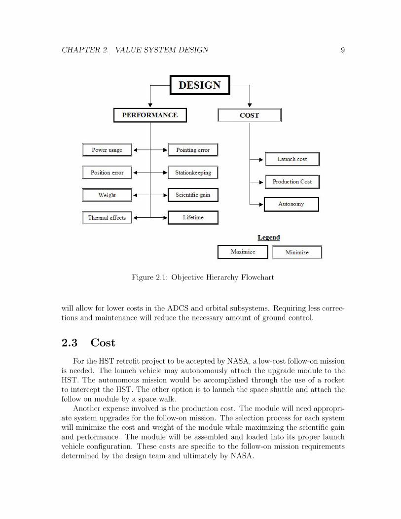
The main objectives for this project are to maximize the performance and mini-mize the cost. For each objective there are many smaller aims that must be evaluated.Table 2.1 lists the objectives for this project. Figure 2.1 shows the entire objectivehierarchy.
2.2 Performance
As each objective is analyzed, a measure of effectiveness is associated with boththe performance and cost parameters. For example, a measure of effectiveness for theADCS is pointing error of the pointing control system. The MOE should be minimizedto achieve greater precision in attitude maneuvers, maximizing scientific performance.Position error is another MOE for the ADCS that should also be minimized. Weightis an important MOE as it affects almost all performance and cost parameters. Forexample, minimizing the weight can directly minimize the launch costs. However, theproduction cost may increase significantly due to the cost of the particular material.Perhaps the material, although lighter, may not maximize the thermal performanceof the spacecraft and its devices.
7

CHAPTER 2. VALUE SYSTEM DESIGN 8
Table 2.1: List of ObjectivesObjectives Brief DescriptionPerformanceScientific Gain Maximize possible scientific missionsLifetime Maximize overall mission durationPower Usage Minimize consumption of powerWeight Minimize weightPosition Error Minimize location errorPointing Error Minimize attitude errorStationkeeping ∆V Minimize fuel usageThermal Effects Minimize thermal damageCostLaunch Cost Minimize cost of launch vehicleProduction Cost Minimize design and manufacturing costAutonomy Maximize satellite-ground independence
Currently in LEO, at 600 km, the Hubble Space Telescope experiences both ex-tremes of thermal effects while completing an orbit. The HST experiences severe coldtemperatures while in eclipse, and high temperatures while facing direct sunlight.These temperatures range from -300 degrees Fahrenheit to +300 degrees Fahrenheit.Currently the HST uses multi-layer insulation (MLI), attached to the outside of thespacecraft to act as a thermal barrier. The MLI consists of several 25 µm thick sheetsof material. For cooling the sensitive infrared (IR) instrument NICMOS, the HSTuses the NICMOS Cooling System (NCS). However, if the HST is moved into an orbitat either L4 or L5, the satellite will constantly be in direct sunlight. Without expe-riencing eclipse there will not be a natural opportunity for HST to cool. The lack ofeclipse could have severe effects on HST’s operations if adequate thermal protectionand cooling systems are not provided.
The radiation effects on the HST will be increased if moved to L4 or L5. TheHST does receive some extra protection from solar radiation when it is in eclipse. Ifcontinually exposed to the sun’s radiation, the effect of the added exposure on HST’sinstruments must be determined.
The HST power subsystem uses solar arrays and batteries. Batteries are used topower the satellite in eclipse. If placed in L4 or L5 the HST would be able to use itssolar arrays at all times, reducing the required capacity of the batteries.
The scientific gain, which is involved with all subsystems, should be maximized.Maximizing scientific gain would make the retrofit mission most desirable to bothpublic and private sectors. The lifetime should be maximized to increase the numberof possible scientific missions. A maximum lifetime may increase cost, but the outputof valuable data will outweigh the extra cost.
The station keeping ∆V should be minimized. A minimum station keeping ∆V
CHAPTER 2. VALUE SYSTEM DESIGN 9
Figure 2.1: Objective Hierarchy Flowchart
will allow for lower costs in the ADCS and orbital subsystems. Requiring less correc-tions and maintenance will reduce the necessary amount of ground control.
2.3 Cost
For the HST retrofit project to be accepted by NASA, a low-cost follow-on missionis needed. The launch vehicle may autonomously attach the upgrade module to theHST. The autonomous mission would be accomplished through the use of a rocketto intercept the HST. The other option is to launch the space shuttle and attach thefollow on module by a space walk.
Another expense involved is the production cost. The module will need appropri-ate system upgrades for the follow-on mission. The selection process for each systemwill minimize the cost and weight of the module while maximizing the scientific gainand performance. The module will be assembled and loaded into its proper launchvehicle configuration. These costs are specific to the follow-on mission requirementsdetermined by the design team and ultimately by NASA.

CHAPTER 2. VALUE SYSTEM DESIGN 10
The operation cost would entail an upgraded power system, communication sys-tem, propulsion system, and scientific package for the follow-on mission. The costassociated with the upgrades will be assessed throughout the design process. TheHST will not be serviced after transfer into its new orbit. The upgrade module is thedeciding factor in determining the follow-on mission’s cost. If the cost is reasonable,the HST follow-on mission could be a feasible alternative to decommissioning theHST in 2010.
2.4 Summary
The construction of a value system design allows different design proposals tobe evaluated by effectiveness. The VSD contains a set of mission objectives andattributed measures of effectiveness. The MOEs are applied to each of the prospec-tive solutions developed in the next chapter. Each design can then be compared todetermine which solves the problem in the most optimal manner.

Chapter 3
System Synthesis
The system synthesis chapter discusses, in detail, the alternatives that are avail-able for each subsystem. This chapter will then explain the effects that each optioncould have on other subsystems. The analysis will be used to narrow the choices andcombine them into “options”, which will then be optimized.
3.1 Orbit Options
A large number of different orbital schemes would be useful in furthering thescience missions of the new Hubble. Each type of orbit has its own advantages anddisadvantages. Maximizing the scientific data collection and minimizing the annualorbit stationkeeping are important to consider when choosing an orbit.
One potential class of orbits is the halo family of orbits around a Lagrange point.A Lagrange or libration point is a state of equilibrium in the gravity field of two largemasses. A small mass can orbit around a Lagrange point. The libration points are theequilibrium solutions of the restricted three-body problem. In any three-body systemthere are five Lagrange points, designated L1, L2, L3, L4, and L5. The locations ofthese points can be seen in Figure 3.1. The Lagrange points are in the same relativelocation for any two mass system. The first three points are collinear with the twolarge masses and represent local minima of gravitational energy. The forth and fifthpoints form equilateral triangles with the two masses and the Lagrange point at thetriangle vertices. In opposition to the first three points, L4 and L5 represent localmaximums of gravitational energy. In the Earth-Sun system, the Sun is much moremassive than the Earth so that it stays nearly fixed in space, and the five Lagrangepoints move around the Sun with the Earth.
A stability analysis of the Lagrange equilibria finds that the collinear Lagrangepoints, L1, L2, and L3, are unstable. Orbiting around these points requires lifelongstationkeeping costs. The upkeep costs are not enough to rule out the possibilityof using one of these points. However, an orbit around L3 would never be able tocommunicate with the Earth, so can safely be ruled out. The L1 and L2 points
11

CHAPTER 3. SYSTEM SYNTHESIS 12
Figure 3.1: Location of Lagrange Points
have other advantages and disadvantages. An L1 orbit is excellent for long-termsolar studies. An L2 orbit is beneficial when solar energy could disrupt sensitiveinstruments. Both of these points are always able to communicate with the Earth.However, a transfer orbit to get into orbit around either of these points is complicatedand costly.
The L4 and L5 points can be shown to be stable if one of the masses is much largerthan the other, such as the Earth-Sun system. Stability is not usually associated withenergy maximums, but when the Coriolis forces introduced by the rotating Earth-Sun reference frame are introduced, the halo orbits around L4 and L5 become stable.In fact, a number of “Trojan” asteroids have been observed orbiting stably aboutthe Jovian L4 and L5 points. Orbits around L4 and L5 would require virtually nostationkeeping; the only major perturbation is solar radiation pressure. However,no satellite has ever been sent to L4 or L5 to confirm this stability. The lack ofdata creates some uncertainty and risk in the orbital conditions. However, it alsoprovides the opportunity to make valuable scientific measurements. Orbits around L4and L5 also provide eclipse-free conditions with constant communication availability.Transferring to L4 or L5 requires only a simple Hohmann phasing maneuver, sincethe two Lagrange points follow the same orbit as Earth.
Another option for a new Hubble orbit scheme is positioning near a Lagrangepoint in the Earth-Moon system, as opposed to the Earth-Sun system. An orbit in theEarth-Moon system would allow for cheaper transfer orbits and easier communicationsdue to the proximity to Earth. However, the Earth-Moon points do not offer asvaluable scientific vantage points as Earth-sun points.

CHAPTER 3. SYSTEM SYNTHESIS 13
A third viable option for Hubble is a heliocentric orbit not at a Lagrange point.A heliocentric orbit could be tailored to a specific mission by varying its location inthe Solar System. The new orbit could be farther out than a Lagrange point or muchcloser to the Sun. The flexibility of a new heliocentric orbit also introduces problems.The Earth and Sun are not in a constant orientation with respect to the spacecraftso solar power and Earth communication quality could vary drastically throughoutthe course of an orbit.
3.2 Attitude Systems
The Hubble Space Telescope already has a fully functional attitude determinationand control system. The only component of this system that would no longer workaway from the Earth is the magnetometer. However, the magnetometer is not integralto the attitude determination of the Hubble, as HST has many redundant determina-tion devices. The current attitude control system is already one of the most accuratesystems ever flown and will continue to be so. Regular maintenance will need to beperformed, as in all other service missions. The only addition that might be neededis a set of external torquers to provide a momentum dumping system. A small setof thrusters would be one solution for this problem and could also be used for orbitmaintenance.
The current Hubble attitude controller may be sufficient for continued opera-tion, but if the upgrade module is to dock with HST autonomously it will requireits own attitude system. The attitude system would have to work in concert withthe new propulsion system to rendezvous successfully with Hubble. The propulsionsystem could be comprised of any standard attitude control system, including reac-tion/momentum wheels, thrusters or control moment gyros. The autonomous dockerwould also need its own attitude determination system, using star trackers, sun sen-sors, or magnetometers.
3.3 Thermal
The most common method of shielding a spacecraft from the thermal and radiationeffects of outer space is to use thermal blankets on the outside of the vehicle. Thermalblankets are most often referred to as multi-layer insulation. MLI is used to insulatethermally against radiative heat transfer. The insulation also provides protectionfrom solar heating and heat transfer among components in the vehicle. MLI can alsobe used to reduce heat loss from the spacecraft. If electric heating of a component isrequired, the reduced heat loss will result in the need for less electric power[18].
MLI mostly consists of 20 to 30 µm thick layers of aluminized Mylar or Kapton.Kapton is used over Mylar for higher temperatures up to 340◦C. For protection against

CHAPTER 3. SYSTEM SYNTHESIS 14
the heat of rocket motors, the outermost layer may be a thin sheet of titanium orstainless steel[18].
Thermal protection can also be provided by optical solar reflectors (OSRs). TheOSRs produce the lowest temperatures when irradiated by solar energy. The reflectorsare created by mounting a highly reflective surface on the outside of the spacecraft andoverlaying it with a transparent cover. The cover material partially absorbs incomingradiation and transmits it to the reflective surface, which reflects the majority of theradiation back into space. The OSRs typically have an infrared (IR) emissivity of 0.8and a solar absorptivity of 0.15[31].
Space radiators are used on spacecraft as heat exchangers. The radiators aremounted on the outside to expel waste heat into outer space. Waste heat often comesfrom electronic heating of components within the satellite, or from a thermal systemsuch as a cryogenic cooler.
Heat pipes are used to transport heat from one location to another. The pipescan transfer heat from one component bay to another or they can send it to a spaceradiator. Heat pipes are hermetically sealed tubes with a wicking device. Capillaryforces are used to draw the fluid from the condenser end to the evaporator end of thepipe. The fluid in heat pipes have a high latent heat of evaporation, allowing for highheat transfer rates and small temperature differences between each end[31].
Cryogenic systems are used for specific instruments such as low-noise amplifiers,superconducting equipment, and IR detectors. Cryogenic systems operate in therange of -271◦C to -150◦C. These systems are divided into two categories, active re-frigeration systems, and expendable cooling systems. Active refrigeration units areused on long duration missions and are based on Stirling or reverse Brayton cycles.Waste heat is rejected to space using a thermal radiator. However, vibration, reliabil-ity, and operating life are critical issues for this device. Expendable cooling systemsare used for short duration missions. The expendable systems use low temperaturefluids to absorb heat and remove it from the spacecraft as a vented gas. These systemsare more reliable and less expensive than active refrigeration units[31].
3.4 Power
Four types of power sources are typically used in spacecraft power systems. Thesetypes include photovoltaic solar cells, dynamic power sources, static power sources,and fuel cells. Photovoltaic solar cells are the most commonly used power sourcesfor Earth orbiting spacecraft. A solar cell converts incident solar radiation directlyinto electrical energy. Static power sources use a heat source, such as plutonium anduranium, to generate electricity. Dynamic power sources also use heat, usually solarradiation, plutonium or enriched uranium, to produce power with the use of Brayton,Stirling, or Rankine cycles. Fuel cells are used on manned missions such as the SpaceShuttle and Apollo.

CHAPTER 3. SYSTEM SYNTHESIS 15
3.4.1 Solar Arrays
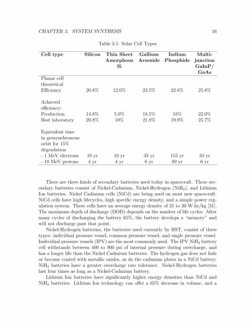
The best source of power for the mission would be photovoltaic solar cells, dueto the fact that the spacecraft will have constant exposure to solar radiation. Onetype of photovoltaic solar cells is crystalline silicon. Crystalline silicon has a 95%absorption, with a planar cell theoretical efficiency of 20.8%, and an achieved efficiencyfor production of 14.8%. The electrical output for an open circuit is 0.55 volts [31],while the electrical output for a short circuit is 0.275-0.3 amps. The equivalent timein geosynchronous orbit for 15% degradation for 1MeV electrons is 10 years and 4years for 10 MeV protons.
Amorphous silicon is another type of photovoltaic solar cell and is arranged ina thin sheet that is flexible and can be rolled up for storage. These cells have aplanar-cell theoretical efficiency of 12%, an achieved efficiency for production of 5%,and 10% efficiency for best laboratory tests. The equivalent time in geosynchronousorbit for 15% degredation for 1 MeV electrons is 10 years and 4 years for 10 MeVprotons.
Gallium Arsenide (GaAs) cells are liquid cooled with a light-conditioning featurethat removes unusable wavelengths from the light spectrum. The planar-cell theo-retical efficiency is 23.5% with an achieved efficiency for production of 18.5% and alaboratory efficiency of 21.8%. The equivalent time in geosynchronous orbit for 15%degradation for 1 MeV electrons is 33 years and for the 10 MeV protons of 6 years.
Indium Phosphide also resists radiation and provides greater end-of-life power fora given area. Indium Phosphide has a planar cell theoretical efficiency of 22.8%, anachieved efficiency for production of 18%, and a best laboratory efficiency of 19.9%.The equivalent time in geosynchronous orbit for 15% degradation for 1 MeV electronsis 155 years and 89 years for 10 MeV protons.
Multijunction gallium indium phosphide/gallium arsenide (GaInP/GaAs) cellsconvert more of the energy spectrum of light to electricity, thus achieving a highertotal conversion efficiency. The GaInP/GaAs cell has a planar cell theoretical effi-ciency of 25.8%, a production-achieved efficiency of 22.0%, and a laboratory efficiencyof 25.7%. Multijunction cells have an equivalent time in geosynchronous orbit of 33years for 15% degradation for 1 MeV electrons, and 6 years for 10 MeV protons.
3.4.2 Batteries
Batteries in spacecraft can either be classified as primary or secondary. Primarybatteries are not rechargeable, and are used for short-duration missions. Secondarybatteries are used in conjunction with solar arrays for power. Solar arrays will be usedand secondary batteries will be required for power storage for this mission. Secondarybatteries can supply power for the electrical load when in eclipse or when the loadexceeds the power of the solar array. In this case, there will be no eclipse, so thebatteries will be used when the power demand exceeds what the solar arrays canprovide.
CHAPTER 3. SYSTEM SYNTHESIS 16
Table 3.1: Solar Cell Types
Cell type Silicon Thin Sheet Gallium Indium Multi-Amorphous Arsenide Phosphide junction
Si GaInP/GaAs
Planar celltheoreticalEfficiency 20.8% 12.0% 23.5% 22.8% 25.8%
Achievedefficiency:Production 14.8% 5.0% 18.5% 18% 22.0%Best laboratory 20.8% 10% 21.8% 19.9% 25.7%
Equivalent timein geosynchronousorbit for 15%degradation- 1 MeV electrons 10 yr 10 yr 33 yr 155 yr 33 yr- 10 MeV protons 4 yr 4 yr 6 yr 89 yr 6 yr
There are three kinds of secondary batteries used today in spacecraft. These sec-ondary batteries consist of Nickel-Cadmium, Nickel-Hydrogen (NiH2), and LithiumIon batteries. Nickel Cadmium cells (NiCd) are being used on most new spacecraft.NiCd cells have high lifecycles, high specific energy density, and a simple power reg-ulation system. These cells have an average energy density of 25 to 30 W-hr/kg [31].The maximum depth of discharge (DOD) depends on the number of life cycles. Aftermany cycles of discharging the battery 65%, the battery develops a “memory” andwill not discharge past that point.
Nickel-Hydrogen batteries, the batteries used currently by HST, consist of threetypes: individual pressure vessel, common pressure vessel, and single pressure vessel.Individual pressure vessels (IPV) are the most commonly used. The IPV NiH2 batterycell withstands between 400 to 900 psi of internal pressure during overcharge, andhas a longer life than the Nickel Cadmium batteries. The hydrogen gas does not fadeor become coated with metallic oxides, as do the cadmium plates in a NiCd battery.NiH2 batteries have a greater overcharge rate tolerance. Nickel-Hydrogen batterieslast four times as long as a Nickel-Cadmium battery.
Lithium Ion batteries have significantly higher energy densities than NiCd andNiH2 batteries. Lithium Ion technology can offer a 65% decrease in volume, and a

CHAPTER 3. SYSTEM SYNTHESIS 17
50% mass decrease over the present day spacecraft battery applications. LithiumIon batteries are relatively new, and not yet available for spacecraft. These batteriesshould become available for use between 2005 and 2010.
Table 3.2: Secondary BatteriesSecondary Battery Specific Energy Density StatusCouple (W*hr/kg)Nickel-Cadmium 25-30 Space-qualified,
extensive databaseNickel-Hydrogen 35-43 Space-qualified, good(individual pressure vessel databasedesign)Nickel-Hydrogen 40-56 Space-qualified for(common pressure vessel GEO and planetarydesign)Nickel-Hydrogen 43-57 Space-qualified(single pressurevessel design)Lithium-Ion 70-110 Under development(LiSo2, LiCF, LiSOCl2)Sodium-Sulfur 140-210 Under development
3.4.3 Power Regulation
The electrical power generated by the solar array must be regulated to prevent bat-tery overcharging and undesired heating. The two main power regulation subsystemsused with photovoltaic solar cells are peak-power trackers (PPT) or direct-energy-transfer (DET) systems.
Peak-power trackers operate in series with the solar array, and change the operat-ing point of the solar array source to the voltage. When the peak power point demandexceeds peak power, the operating point changes to the voltage side of the array, andthe tracker tracks the peak-power point. The array voltage increases to its maximumpower point, and the converter transforms the input power to equal the output powerat a different voltage and current. The PPTs have advantages for missions under 5years that require more power at beginning of life (BOL) than at end of life (EOL).Direct Energy Transfer systems run in series with the solar array and require a shuntregulator to control the array current. The shunt is typically located at the arrayand carries the current away from the battery subsystem when power is not needed.The DET systems are more efficient than PPT, due to the smaller energy dissipation,lower mass, and fewer parts.

CHAPTER 3. SYSTEM SYNTHESIS 18
3.4.4 Electrical Bus Voltage Control
There are three types of electrical bus voltage control systems, which includeunregulated, quasi-regulated, and full-regulated systems. Load bus voltages vary inan unregulated system. In an unregulated system, the bus-voltage regulation derivesfrom battery regulation, which varies about 20% from charge to discharge [31]. Theload bus voltage is the voltage of the batteries. Quasi-regulated subsystems regulatethe bus voltage during battery charge, but not during discharge. A charger is inseries with the battery. Quasi-regulated subsystems have a low efficiency and highelectromagnetic interference if used with a peak-power tracker. A fully regulatedsystem is inefficient, but will work on a spacecraft that requires low power and ahighly regulated bus. A fully regulated system uses charge regulators during thecharge and discharge cycles of the battery. It behaves like a low-impedance powersupply when connected to loads, simplifying design integration of the subsystems.
3.5 Propulsion
Space propulsion systems perform three main functions: lift the launch vehicle andits payload from the launch pad, place the payload into low-Earth orbit, and transferpayloads from LEO into higher orbits. Propulsion systems also provide thrust forattitude control and orbit corrections. Two measures of a spacecraft’s propulsionsystem are the thrust, F , and the specific impulse, Isp. Thrust is the amount offorce applied to the rocket based on the expulsion of gases. Specific impulse is ameasure of the energy content of the propellants, and how efficiently it is convertedinto thrust[31]. Space propulsion systems are comprised of four main types: chemical,electric, cold gas, and advanced.
Chemical propulsion systems can be divided up into three basic categories: solid,liquid, and hybrid. The aforementioned terminology refers to the physical state ofthe stored propellants. Rockets using solid propellants are called motors and rocketsusing liquid are called engines or thrusters. Solid rocket motors have a high thrustvalue associated with them, so these motors are used only for launch or orbit in-sertions requiring a high ∆V . However, the benefit of using solid rocket motors isthey are simple, reliable, and inexpensive systems. The next chemical propulsion sys-tem that is slightly more massive than the solid rocket motor is a hybrid propulsionsystem. Hybrid rockets are more complex than solid systems; they compare in perfor-mance to liquid systems while requiring only half of the “plumbing.” This reductionin complexity vastly reduces the overall system weight and cost, while increasing itsreliability. Hybrid chemical propulsion systems store the propellants in a differentform making the rocket safer, cleaner, and better performance [24].
Liquid rocket engines store the propellants in tanks as liquids. On demand, thefuel can be fed into the combustion chamber by gas pressurization or a pump. Liquidrocket engines are either monopropellant, bipropellant, or duel mode systems. Mono-

CHAPTER 3. SYSTEM SYNTHESIS 19
Table 3.3: Properties of Common Propellants [31]Type Energy Isp (s) Thrust Range (N)Cold gas High pressure 50-75 0.05-200Liquid Monopropellant Chemical 150-225 0.05-0.5Liquid Bipropellant Chemical 350-430 5-5000000Resistojet Resistive heat 150-700 0.005-0.5Arcjet Electric heat 450-1500 0.05-5Ion Electrostatic 2000-7000 0.000005-0.5Colloid Electrostatic 1200 0.000005-.05Pulsed plasma Magnetic 1500 0.000005-0.005Pulsed inductive Magnetic 2500 2-200
propellant engines are the most widely used type of propulsion for spacecraft attitudeand velocity control. Monopropellant systems are both simple and inexpensive; how-ever, they provide a relatively low output of ∆V . Bipropellant engines react a fuelwith an oxidizer to achieve a much higher performance. Bipropellant engines involveadditional system complexity and cost, yet they can be used to perform any necessarymaneuver. Dual mode systems combine the use of bipropellant and monopropellantto achieve an even higher performance, allowing for accurate orbit maneuvering [31].
Electric propulsion systems use electrical power to accelerate the working fluid toproduce useful thrust. There are three classes of electric propulsion systems: elec-trostatic, electromagnetic, and electrothermal. In electrostatic propulsion the thrustis produced by accelerating charged particles in an electrostatic field. Electrostaticpropulsion includes three types of devices: electron bombardment thrusters, contaction thrusters, and field emission/colloid thrusters. The first two involve the produc-tion and acceleration of separate ions and are forms of ion propulsion. The third typeinvolves the production and acceleration of charged liquid droplets. Only the elec-tron bombardment thrusters have been used operationally aboard spacecraft. Withelectromagnetic propulsion the propellant is accelerated after having been heated toa plasma state. There are several subcategories of electromagnetic propulsion, in-cluding magnetoplasmadynamic thrusters, pulsed-plasma thrusters, and Hall Effectthrusters. Lastly, in an electrothermal propulsion system electrical energy is usedto heat a suitable propellant, causing it to expand through a supersonic nozzle andgenerate thrust. Two basic types of electrothermal thrusters are in use today: theresistojet and the arcjet. In both, material characteristics limit the effective exhaustvelocity to values similar to those of chemical rockets[11]. In electric propulsion sys-tems there is no fundamental limit (other than the speed of light) to the exhaustvelocity that can be obtained. However, the material properties and power requiredmay reach a point where further acceleration is either impossible or too expensive.
Cold gas propulsion uses a controlled, pressurized gas source and a nozzle. It

CHAPTER 3. SYSTEM SYNTHESIS 20
represents the simplest form of rocket propulsion. There are many applications wheresimplicity is more important than performance. Cold gas systems are only used fororbit maintenance and attitude control due to their low performance. These systemsare rather large for their level of performance; however, they are simple, reliable, andinexpensive[31].
Advanced propulsion systems are still experimental concepts. These space systemsare expected to have optimal performance and assist in allowing for more efficientspace missions. A few of these propulsion systems include advanced chemical propul-sion systems using tripropellants, forms of nuclear propulsion, antimatter propulsion,and sails (solar, light, microwave, and magnetic).
3.6 Communications
In LEO, the HST uses the TDRSS satellites to communicate with ground stationson Earth. Hubble also can use the Deep Space Network (DSN) in case there is anoutage of the normal communication service. If moved to L4 or L5 the HST could stilluse the DSN to communicate with Earth. The HST could use S-, X-, Ka- frequencybands in order to communicate with the Earth based ground stations or satelliteconstellations.
For deep space communications, the S-band and X-band regions are chosen basedon relatively low noise and relatively low attenuation (signal weakening) through theEarth’s atmosphere. The wavelength of a radio signal is inversely proportional toits frequency. S-band has the largest wavelength, followed by X-band, and Ka-bandwavelengths. There are sources of noise, such as noise emitted from the sun, fromplanets, and from the Galaxy itself. These noises are somewhat lower at X-band andKa-band than at S-band [27].
The power efficiency and the equipment size are two factors that enter into thedesign of spacecraft. Generally, the order of efficiency (requiring less spacecraft powerfor a given amount of radio output power) is S-band, X-band, then Ka-band. Also,some radio equipment sizes (for example, antenna diameters or the dimensions of thewave guides that carry signal to the antenna) are proportional to the wavelength. So,Ka-band equipment is smaller than X-band. The size is important when every gramof mass is counted in a spacecraft design [27].
The high-gain antenna sizing is important for relaying the data to and from L4 orL5. Data rate is another concern of the communication system, which will determinehow often communications need to be established. If a high data rate is required forthe follow on mission, then the DSN is going to be the optimal choice.

CHAPTER 3. SYSTEM SYNTHESIS 21
3.7 Structures
When HST is upgraded, multiple structural changes will occur. New solar panelsmay be installed, the propulsion system and attitude control devices must be at-tached, and component bays may be exchanged. The structural upgrades will havethe greatest effect on the following objectives: pointing error, mass, and cost. Forthe most part structural considerations will not be a driving factor in retrofit missiondesign. More likely the mission design will be the defining factor in the structuralneeds.
3.7.1 Solar Arrays
By moving HST out of an Earth orbit, the negative effect the solar panels havehad on pointing error and jitter will no longer occur. While in Earth orbit, HSTexperiences large temperature gradients while traveling in and out of eclipse. TheHST’s structure will grow and shrink during each orbit due to these temperaturegradients. The rapid change in structure causes the craft to jitter, or shake, as thesolar arrays react to the thermal gradients (∆T ). The phenomenon described aboveis experienced by all components on the telescope. Since the solar arrays are largeand thin, they experience a more significant deformation than most parts of thespacecraft. The solar array structure can not compensate for this large jitter effect.The original HST mission had a major problem with jitter. Deviations were expectedto be less than 0.007 arcsec, but were found to be 0.2 arcsec, which is nearly 30times the allowable jitter. The problem was later fixed during a servicing missionby replacing the solar array structure. The retrofit mission will completely minimizethis problem by moving HST to a heliocentric orbit, where the temperature is nearlyalways constant. Therefore HST’s new solar arrays will either be identical to thecurrent arrays or a smaller scaled down version of what is there. If no new arrays arerequired, the production cost would be greatly reduced. If newer smaller arrays areused, the total mass would be reduced.
3.7.2 Other Structural Components
The HST will need to have the propulsion and attitude control devices attached toits existing structure to make this initial orbit change, and to maintain the attitudewhile in its new orbit. These adaptations will be bolted on to the original structureof HST. All structures will be designed to be as lightweight and strong as possible.The main concern will be to minimize mass, while keeping the cost within budgetconstraints. Any new instrument containers will be designed to have similar massproperties to the current system. Table 3.4 shows many options for materials thatwill be considered in each of these applications.

CHAPTER 3. SYSTEM SYNTHESIS 22
Table 3.4: Properties for Commonly Used Materials [17]Material Alloy and Form ρ Ftu Fcy E e α
103 106 106 109 % 10−6
Kg/m3 N/M2 N/M2 N/m2 ◦CAluminum 2219-T851 1” Plate 2.85 420 320 72 7 22.1
6061-T6 Bar 2.71 290 240 68 8 22.97075-T73 Sheet 2.8 460 380 71 10 22.1
Steel 17-4PH H1150z Bar 7.86 860 620 196 16 11.2Heat-Res. Alloy A-286 2” Bar Plate 7.94 970 660 201 12 16.2
Inconel 718 4”Bar 8.22 1280 1080 203 12 12.2Magnesium Az31B H24 Sheet 1.77 270 165 45 6 25.4Titanium Ti-6Al-4V An. Plate 4.43 900 855 110 10 8.8Beryllium AMS 7906 Bar 1.85 320 - 290 2 11.5
3.8 Science Missions
Hubble can house a total of eight science instruments, four that can be alignedwith the Telescope’s main optical axis and four that can be mounted radially. Thecurrent axially mounted instruments for Hubble are the Space Telescope ImagingSpectrograph (STIS), Advanced Camera for Surveys (ACS), Near Infrared Cameraand Multi-Object Spectrometer (NICMOS), and the Corrective Optics Space Tele-scope Axial Replacement (COSTAR) [21]. The radially mounted instruments includethe Wide Field and Planetary Camera 2 (WFPC2) and the three Fine GuidanceSensors (FGS). There is one final service mission that was planned for the HST inmid-2005. However, due to current shuttle problems, this service mission will nottake place. The cameras have all been built and are ready for launch. For this mis-sion, Service Mission 4 (SM4), two of the instruments were supposed to be replaced.The WFPC2 would be replaced by the Wide Field Camera 3 (WFC3) and COSTARwould be replaced with the Cosmic Origin Spectrograph (COS). The COSTAR will nolonger be needed since all instruments have their own corrective optics. The retrofitmission will make all the changes that were supposed to happen during SM4.
There are many possible missions that can be developed for Hubble as an al-ternative to decommissioning. All the cameras can be removed and replaced withinstruments that are new and innovative. Another option is to replace nothing, keep-ing Hubble with its current missions. A third possibility includes using the currentcameras for new missions. Possible missions for the Hubble will be chosen and opti-mized in subsequent chapters. However, the possibilities must first be explored.
Each of the onboard cameras has different masses, dimensions, and capabilities.These differences, described below, are described completely in Reference [20].
The ACS, shown in Figure 3.2, is 397 kg with dimensions of 0.9 × 0.9 × 2.2 mand has a wavelength range of 115-1050 nanometers. The observations performed by

CHAPTER 3. SYSTEM SYNTHESIS 23
this camera includes searching for extra-solar planets, observing weather and auroraeon planets in this solar system, conducting vast sky surveys to study the nature anddistribution of galaxies, searching for galaxies and clusters of galaxies in the early uni-verse, searching for hot stars and quasars, and examining the galactic neighborhoodsaround bright quasars.
Figure 3.2: Diagram of the Advanced Camera for Surveys [20]
The cryogen was depleted for NICMOS (Figure 3.3) in 1998. In Service Mission3B (SM3B), the NICMOS cooling system (NCS) was installed to keep NICMOSrunning. The NICMOS is 391 kg and its dimensions are 2.2 × 0.88 × 0.88 m. It

CHAPTER 3. SYSTEM SYNTHESIS 24
can produce infrared (IR) imaging and limited spectroscopy (1.0 to 2.5 microns). Itsobservations include prostellar clouds, young star clusters and brown dwarfs, obscuredactive galaxy nuclei, temporal changes in planetary atmospheres, young protogalaxies,and supernovae at high redshift used to time the acceleration of the expansion of theuniverse.
Figure 3.3: Diagram of the Near Infrared Camera and Multi-Object Spectrometer[20]
The STIS (Figure 3.4) was added to Hubble to give a new two-dimensional capabil-ity to its spectroscopy. The camera has a mass of 374 kg and measures 2.2×0.98×0.98m. It can be used in searching for massive black holes by studying star and gas dynam-ics around the centers of galaxies, measuring the distribution of matter in the universeby studying quasar absorption lines, watching stars forming in distant galaxies, map-ping fine details of planets, nebulae, galaxies and other objects, imaging Jupiter-sizedplanets around nearby stars, and obtaining physical diagnostics. These diagnosticsinclude chemical composition, temperature, density and velocity of rotation or inter-nal mass motions in planets, comets, stars, interstellar gas, nebulae, stellar ejecta,galaxies and quasars.
The WFC3, Figure 3.5, will acquire WFPC2’s job as the “workhorse” of the HST.It will use improved Charged Couple Device (CCD) and optical coating technology.

CHAPTER 3. SYSTEM SYNTHESIS 25
Figure 3.4: Diagram of the Space Telescope Imaging Spectrograph [20]
Its mass is 281 kg with dimensions of 1 × 1.3 × 0.5 m. It is a multitask camerathat can take a wide-field picture of the galaxy and at the same time concentrate onthe galaxy nucleus to measure light intensity and take photographic close-ups. Thiscamera can make measurements while other instruments continue observing. Thereare many applications for the WFC3 including tests of cosmic distance scales anduniverse expansion theories to specific star, supernova, comet and planet studies.This camera can be used to search for black holes, planets in other star systems,atmospheric storms on other planets and the connection between galaxy collisionsand star formation.
The Cosmic Origins Spectrograph (COS), shown in Figure 3.6, will replace COSTAR.It is a medium resolution spectrograph that can observe near- and mid- ultraviolet(UV) wavelengths. Possible observations include high energy activities such as thosein hot stars and quasi-stellar objects. The UV region is also good for viewing thecomposition and character of the interstellar medium (IM).
There are three FGSs (Figure 3.7) on Hubble to perform astrometry. Two of thesensors lock onto guide stars while the third measures the position of stars in relation

CHAPTER 3. SYSTEM SYNTHESIS 26
Figure 3.5: Diagram of the Wide Field Camera 3: Schematic on left, CAD conceptionof WFC3 on right [21]
to other stars. The sensors are able to find and measure stars as faint as 18 apparentmagnitude. Each fine guidance sensor is 220 kg with dimensions of 0.5 × 1 × 1.6 m.The sensors can measure 10 stars in 10 minutes with an access field of view of 60arcmin2. The main goal of the FGSs is to measure distances to stars. However, theyare also used to detect planets by watching for gravitational effects on nearby stars.The FGSs are used to improve the mass/luminosity relations at the lower end of themain sequence. The main sequence is a diagonal band from top left corner to bottomright corner of the Hertzsprung Russell diagram. The band contains about 90% ofall known stars. The stars evolve into and then off of the main sequence during theirlifetime.
Keeping these cameras on Hubble and moving it to a new location is one possi-bility. Moving HST to L4 or L5 has been considered, which will put it in constantsunlight. In this case it may be easier to remove the IR camera, NICMOS, andthe NCS and replace it with a more advanced computer or perhaps a larger antenna.There is a possibility of replacing this bay with a camera more compatible with findingnear-Earth asteroids. The purpose of this mission will be to track and give forewarn-ing about potentially cataclysmic objects hurtling towards Earth. An existing camerathat has potential for this mission is the Space Based Visible (SBV). The possibilityof using this camera will be explored further later in the paper.
The Hubble has other instruments and capabilities in addition to its current mis-

CHAPTER 3. SYSTEM SYNTHESIS 27
sions. It is equipped with magnetometers that can send information about solarmagnetic properties. Also, at L4 or L5, HST will be able to give valuable informationabout the orbital perturbations at these locations. At this time, information aboutthese two Lagrange points is theoretical.
In a new orbit at L4 or L5, the HST will have many missions, including themissions performed with ACS, STIS, WFC3, COS, and FGS. Hubble will also beable to study magnetic properties of the Sun and the perturbations of the Lagrangepoint. However, the main mission for the new Hubble will be to look for near-EarthAsteroids. Further evaluation will be made in subsequent chapters to see if thesemissions are feasible for the HST.

CHAPTER 3. SYSTEM SYNTHESIS 28
Figure 3.6: Diagram of the Cosmic Origins Spectrograph [20]

CHAPTER 3. SYSTEM SYNTHESIS 29
Figure 3.7: Diagram of the Fine Guidance Sensors [20]
The instruments aboard Hubble for the retrofit mission are the ACS, STIS, andFGS. Also for this design, the instruments COSTAR and WFPC2 will need to bereplaced by COS and WFC3 respectively. Service mission 4 was cancelled and there-fore, this design must take into account the upgrade of these instruments. The maingoal of the aforementioned instruments is to learn the origins of the universe. Thereare still many questions surrounding the universe’s origins, and Hubble strives to findanswers everyday. Even though it has been in operation fourteen years, it is still send-ing back new information through its pictures. Papers are constantly being publishedon information from the Hubble. Keeping these instruments and their missions alsomeans the Hubble will act as a counterpart to the James Webb Telescope. Thoughthe James Webb Telescope may be newer and more advanced, it only studies in theinfrared of the universe. These instruments on Hubble can then fill in the gaps where

CHAPTER 3. SYSTEM SYNTHESIS 30
IR is not enough. In addition, there will be a large gap of time between the proposedend of the Hubble and the launch of the James Webb, which may now be as lateas 2017. Astronomers would then have no observatory in space, which would stopinstrument development and erode observational teams.
In addition to Hubble’s current missions, sending it to L4 or L5 would be veryuseful. The information known about these locations is only theoretical. Sending aspacecraft to L4 or L5 will test these theories, and will give valuable information forfuture missions to these locations. Positioning at Lagrange points 4 or 5 will determineif a stable orbit can truly be achieved around these gravitational maximums. Theperturbations associated with the chosen Lagrange point can also be determined. Inaddition, the onboard magnetometer (currently using the Earth’s magnetic field) canbe used to study the magnetic properties of the sun at the new location.
The new mission that will be developed in greater detail in subsequent chaptersis asteroid detection. Detection of asteroids may provide early warning in the eventthat an asteroid’s orbit will collide with the Earth. Then perhaps, preparations canbe made to prevent large-scale destruction. Using HST to find Near Earth Objects(NEO) will prove advantageous for reasons detailed below.
The NEOs are defined as bodies in space whose orbit approaches the path ofEarth to within 0.3 AU (Astronomical Units). The two types of NEO are asteroids,made mostly of carbon-rich materials, silicate rock and metal, and comets, composedmostly of ice and dust. Today, the orbits of 500 Near Earth Asteroids (NEA) thatare larger than 1 km in diameter have been identified out of an estimated 2000 [9].There are then at least 1500 asteroids that could have a cataclysmic effect on theEarth. NEAs are estimated to have a 10-100 million year lifetime. Therefore it wouldbe expected that the population of NEAs would diminish from collisions with innerplanets, or from being ejected from the inner solar system into the Oort cloud or fromthe solar system altogether by near misses with planets. However, it appears thatthese Near Earth Asteroids are constantly replenished.
An advantage of using a space telescope, such as the Hubble Space Telescope, is itsvantage point. Many asteroids have orbits smaller than the Earth (these asteroids arecalled Atens) and can only be observed by space telescopes because they are alwayson the daytime side of the Earth, as seen in Figure 3.8. A space telescope positionedat L4 or L5 could see between the Earth and the Sun and also behind the Sun.
Currently, NEOs 1 km in diameter and bigger are tracked; however, smaller NEOscan still do significant damage. Asteroids will sometimes land in the ocean causingtsunamis. These are giant waves that travel large distances over ocean and land.Objects that crash on land can cause craters. The impacts cause rock to be ejectedmany kilometers past the point of impact. Crater impacts can also cause earthquakes,blast waves, and wildfires. Weak asteroids and comets that break apart explosivelyin the air cause blast waves. These NEOs never reach the land, but can do signif-icant damage all the same. Larger impacts can sometimes cause a climate change,sometimes called a “nuclear winter.” These impacts throw up dust and gas into the

CHAPTER 3. SYSTEM SYNTHESIS 31
Figure 3.8: Orbit of an Aten Asteroid
atmosphere, which can rapidly alter the Earth’s climate.Many scars from past impacts have been smoothed over by the dynamic planet;
however, evidence remains and gives us insight to potential dangers posed by NEOs.Every day, hundreds of meteorites fall to Earth’s surface. Most of them go unnoticed,but they can sometimes damage personal property, as seen in Figure 3.9. On March28, 2003, people of Illinois, Indiana, Ohio and Wisconsin witnessed a disintegratingmeteorite flash across the sky. Fragments fell, mostly in southern Chicago suburbs,striking homes and cars. Over 500 fragments were collected from the area. Since1928, this fall was the ninth recorded in Illinois.
Figure 3.9: Damage on Car from Meteorite [9]
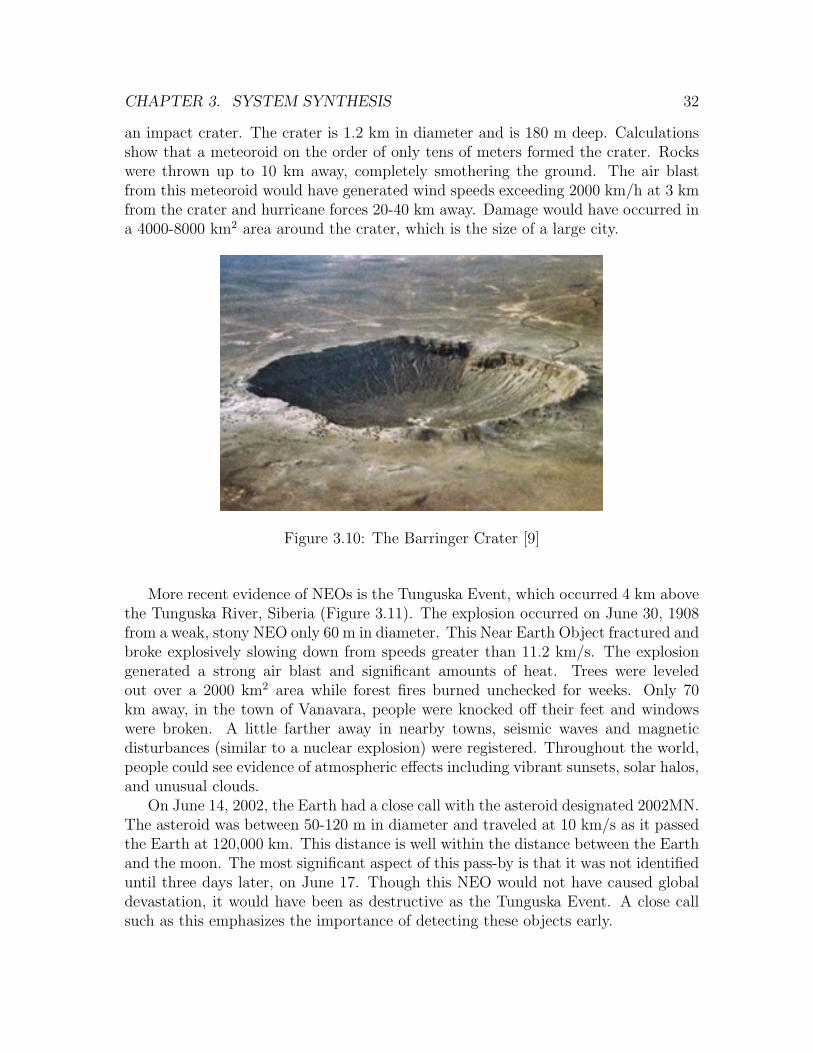
The Barringer Crater in Arizona (Figure 3.10), formed 49,000 years ago, shows
CHAPTER 3. SYSTEM SYNTHESIS 32
an impact crater. The crater is 1.2 km in diameter and is 180 m deep. Calculationsshow that a meteoroid on the order of only tens of meters formed the crater. Rockswere thrown up to 10 km away, completely smothering the ground. The air blastfrom this meteoroid would have generated wind speeds exceeding 2000 km/h at 3 kmfrom the crater and hurricane forces 20-40 km away. Damage would have occurred ina 4000-8000 km2 area around the crater, which is the size of a large city.
Figure 3.10: The Barringer Crater [9]
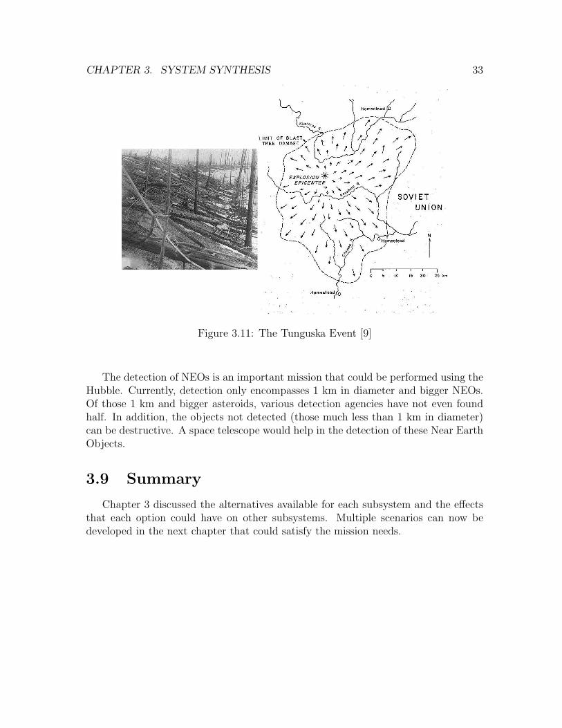
More recent evidence of NEOs is the Tunguska Event, which occurred 4 km abovethe Tunguska River, Siberia (Figure 3.11). The explosion occurred on June 30, 1908from a weak, stony NEO only 60 m in diameter. This Near Earth Object fractured andbroke explosively slowing down from speeds greater than 11.2 km/s. The explosiongenerated a strong air blast and significant amounts of heat. Trees were leveledout over a 2000 km2 area while forest fires burned unchecked for weeks. Only 70km away, in the town of Vanavara, people were knocked off their feet and windowswere broken. A little farther away in nearby towns, seismic waves and magneticdisturbances (similar to a nuclear explosion) were registered. Throughout the world,people could see evidence of atmospheric effects including vibrant sunsets, solar halos,and unusual clouds.
On June 14, 2002, the Earth had a close call with the asteroid designated 2002MN.The asteroid was between 50-120 m in diameter and traveled at 10 km/s as it passedthe Earth at 120,000 km. This distance is well within the distance between the Earthand the moon. The most significant aspect of this pass-by is that it was not identifieduntil three days later, on June 17. Though this NEO would not have caused globaldevastation, it would have been as destructive as the Tunguska Event. A close callsuch as this emphasizes the importance of detecting these objects early.
CHAPTER 3. SYSTEM SYNTHESIS 33
Figure 3.11: The Tunguska Event [9]
The detection of NEOs is an important mission that could be performed using theHubble. Currently, detection only encompasses 1 km in diameter and bigger NEOs.Of those 1 km and bigger asteroids, various detection agencies have not even foundhalf. In addition, the objects not detected (those much less than 1 km in diameter)can be destructive. A space telescope would help in the detection of these Near EarthObjects.
3.9 Summary
Chapter 3 discussed the alternatives available for each subsystem and the effectsthat each option could have on other subsystems. Multiple scenarios can now bedeveloped in the next chapter that could satisfy the mission needs.

Chapter 4
System Analysis
The system analysis chapter evaluates and develops multiple scenarios from thealternatives in Chapter Three. These scenarios will be put together using a Chinesemenu approach. This approach is accomplished by mixing and matching the possibleoptions for each subsystem to build a variety of complete systems. Each of thescenarios will be able to satisfy the mission needs. Once developed, the scenario isthen evaluated to compare the advantages and disadvantages of each configuration.
4.1 Options for Retrofit Mission
Considering the various options for each of the subsections, there are many differ-ent overall missions that can be put together. The following is a description of threepossible scenarios, which have selected one choice from each subsystem to create awhole system. The following chapter will optimize these systems.
4.1.1 Option 1
The full system presented in Table 4.1 is the first option for the Hubble retrofitmission. Option 1 moves the HST to Lagrange point 4, leading the Earth in its orbit.The propulsion for this system is provided by an ion propulsion engine. The additionof extra multi-layered insulation to the existing multi-layered insulation, will insulatethe craft from the constant exposure to the sun’s radiation. The constant sunlight atL4 allows for a smaller solar array to take the place of the existing array. The lack ofeclipse also creates a lower need for energy storage, so smaller batteries would replacethe existing batteries.
The system option 1 has many advantages and disadvantages. These can be seenin Table 4.2.
The benefits of stationing at Lagrange point 4 are that HST will be in constantexposure to solar radiation, providing a continuious amount of power. Lagrange point4 will also offer a field of view that cannot be obtained from the Earth. Batteries could
34

CHAPTER 4. SYSTEM ANALYSIS 35
Table 4.1: Full System Option 1Subsystem OptionLocation L4Propulsion Ion propulsion engineThermal protection More multi-layer insulationPower Generation Replacement solar cellsPower Storage Replacement batteries
be smaller due to the less required amount of stored energy. If HST is stationed inLagrange point 4, then the first study of the point’s characteristics could be performedto compare with theory. The transfer to L4 would require less time compared to anL5 orbit transfer. Lagrange point 4 however has some disadvantages. There is theunderlying possibility of a dust cloud encompassing the region of L4. L4 leads Earthin rotation about the sun, therefore it would require more ∆V than an L5 orbittransfer. Also, it is unknown if the point is actually stable, as theory states.
An ion propulsion system has considerably less mass than chemical propellantsystems. The ion propulsion system can also burn for longer periods of time. A slowacceleration rate of ion engines have no impact loads on enclosed subsystems. Ionengines are more economical than chemical thrusters by a factor of ten[2]. However,the ion plume can re-enter the spacecraft and damage instruments. In addition, ionpropulsion systems require more time to accelerate to design speeds. If not properlyneutralized upon discharge, the ions from the engine could induce a charge on theHST.
Additional multi-layer insulation would provide more protection from the Sun’stemperatures and radiation. The cost would be reduced by adding to the existingMLI rather than revamping the entire insulation system. More MLI would complicatean autonomous retrofit procedure and increase the time of the upgrade.
Replacing the solar cell arrays would provide more efficient arrays for the newmission. A new solar cell array would last longer, with less degradation. New tech-nology could also be incorporated into the new cells for better efficiencies. The newsolar arrays would require the structure to be redesigned to ensure stability. Newarrays would complicate an autonomous mission. In addition, the new solar arrayswould increase the cost of the new mission.
Replacing the batteries would provide additional space within HST for otherequipment, due to the reduction in size. The new batteries would decrease the totalweight of the retrofitted HST. The new batteries could be more efficient and possessa longer lifetime. Disadvantages for new batteries would include an increased costand a complicated autonomous mission.

CHAPTER 4. SYSTEM ANALYSIS 36
Table 4.2: Option 1 Advantages and Disadvantages
Subsystem Option Advantages DisadvantagesL4 Less transfer time than L5 More costly transfer
Potentially more dust
Ion Propulsion system Low mass propulsion system Longer acceleration timesExhaust plume/spacecraft interaction
Extra MLI More solar protection High costs
New solar cells Longer lifetime Higher costMore launch massPossible structure redesign
Replacement batteries Reduced system mass Higher costAdded lifetime Added launch mass
4.1.2 Option 2
The full system presented in Table 4.3 is a second option for the Hubble retrofitmission. Option 2 moves the HST to Lagrange point 5, trailing the Earth in its orbit.The propulsion for this system will be provided by resistojet thrusters. Optical solarreflectors will block the heat and radiation emitted by the sun. The constant sunlightat L5 will allow the existing solar cells to produce enough power to operate the newHST. The lack of eclipse reduces the need for large amounts of energy storage, so thebatteries already on the Hubble will be replaced with fewer, smaller batteries.
Table 4.3: Full System Option 2Subsystem OptionLocation L5Propulsion Resistojet thrustersThermal protection Optical solar reflectorsPower Generation Existing solar cellsPower Storage Replacement batteries
The system option 2 has many advantages and disadvantages. These can be seenin Table 4.4.
The location of this mission is L5. Lagrange point 5 requires less fuel to getthere than L4, making it less expensive. However, it takes longer to get there. An

CHAPTER 4. SYSTEM ANALYSIS 37
advantage of L5 over L4 is that there may be less dust in L5. In the Jupiter-SunLagrange points, there are more Trojan asteroids in the leading Lagrange point (L4)than in the trailing (L5) [3]. The discrepancy is not explained by any current theories.However, if this is true for the Jupiter-Sun Lagrange points, it may also be true forthe Earth-Sun system, leading to less dust in the L5 location.
Resistojets are a type of electrothermal propulsion. They have the desirable qual-ity of having minimal exhaust plume interaction which would have less adverse effecton the optics. However, this propulsion system has a longer mission time. Resistojetsalso have a low thrust.
Optical Solar Reflectors would have more effective solar protection. However, theyare massive, which would add structure and mass. An advantage of reflectors is thatthey are relatively inexpensive.
Using the existing solar arrays would reduce the cost and launch mass for theretrofit mission. They may be deteriorated due to previous use which would makethem closer to failure, reducing the mission lifetime.
Option 2 calls for the use of new batteries. New batteries will reduce the mass ofHST. It would also be wise to use new batteries since the old batteries are closer tofailure. The old batteries are designed to be replaceable. New batteries would addcost and launch mass.
Table 4.4: Option 2 Advantages and Disadvantages
Subsystem Option Advantages DisadvantagesL5 Less expensive transfer Longer transfer time
Potentially less dust
Resistojet thrusters Low exhaust plume interaction Long mission timeLow thrust
Optical solar reflectors More effective solar protection HeavyExtra structurePossible blockage of optics
Existing solar cells Reduced cost Reduced lifetimeReduced launch mass
Replacement batteries Reduced system mass Added costAdded lifetime Added launch mass

CHAPTER 4. SYSTEM ANALYSIS 38
4.1.3 Option 3
The full system presented in Table 4.5 is a third option for the Hubble retrofitmission. Option 3 moves the HST to Lagrange point 5, trailing the Earth in its orbit.The propulsion for this system will be provided by a Mini-Magnetospheric PlasmaPropulsion (M2P2). The M2P2 is a type electromagnetic propulsion system. Thermalprotection for this system will be provided by a replacement covering of MLI. Theconstant sunlight at L5 and low power requirements of the M2P2 system will allowthe existing solar cells to produce enough power to operate the new HST. For ease ofupgrade, the existing batteries will be used.
Table 4.5: Full System Option 3Subsystem OptionLocation L5Propulsion M2P2Thermal protection Replace MLIPower Generation Existing solar cellsPower Storage Existing batteries
The system option 3 has many advantages and disadvantages. These can be seenin Table 4.6.
As in design option 2, the location of this system is L5. L5 requires less fuel toget there than L4, and makes it a less expensive transfer. However, it would takelonger to get to L5 which would have an impact in the mission lifetime. One of theadvantages of L5 over L4 is that there may not be as much dust in L5, which wasdiscussed in design option 2.
Mini-Magnetospheric Plasma Propulsion is a potentially revolutionary plasmapropulsion concept that could enable spacecraft to travel at unprecedented speedsof 50 to 80 km s−1 or could enable travel between the planets for low power require-ments [29]. The high efficiency and specific impulse attained by the system are dueto its utilization of ambient energy, in this case the energy of the solar wind, toprovide enhanced thrust. The ability for a spacecraft to couple to the solar wind isproduced through a large-scale magnetic bubble or mini-magnetosphere. The bubbleis generated by the injection of plasma into the magnetic field supported by solenoidcoils on the spacecraft. This inflation of the mini-magnetosphere is driven by an elec-tromagnetic process, so that the material and deployment problems associated withmechanical sails and other devices are eliminated.
From the laboratory tests it has been shown that plasma can be produced withexcellent confinement up to the point where the chamber wall interactions dominatethe physics [29]. A magnetic field of 0.1 Tesla (stronger than Earth’s magnetic field bya factor of 1000) could be generated by a conventional solenoid for a given spaceship.Tests have also shown that a helicon plasma source is amazingly simple and with a
CHAPTER 4. SYSTEM ANALYSIS 39
bottle of just 3 kg (6.6 lb) of Helium as the plasma fuel, the magnetic bubble couldbe operated for three months. The magnetic bubble itself would be about 30 to 60km (18-36 mi) in diameter as the magnetic field lines would be dragged out with theinjection of the plasma [1] [25]. Utilizing the power in the solar wind is enough topropel a 300-pound spacecraft at 180,000 mph, or 4.3 million miles a day, faster thanthat of the space shuttle by a factor of ten [25].
Mini-Magnetospheric Plasma Propulsion has many advantages to performing amission to L5. It is a relatively inexpensive, low mass propulsion system requiringonly a small amount of plasma fuel. M2P2 can also provide substantially shortenedtravel time to L5 and could enable this for a low power requirement. Although it isextremely efficient it is still only in early stages of development.
As mentioned in design option 1, the addition of more MLI would provide moreprotection from the Sun’s temperatures and radiation. The MLI is the most commonmethod of shielding a spacecraft from the thermal and radiation effects of outer spaceis by use of thermal blankets on the outside of the vehicle. The Hubble currently usesMLI. The insulation also provides protection from solar heating and heat transferamong components in the vehicle. The MLI can also be used to reduce heat lossfrom the spacecraft. The HST currently goes in and out of eclipse as it orbits.However, stationing the HST about L5 would always keep the spacecraft in constantSun exposure. Upgrading the multi-layer insulation on the HST would be beneficialto ensure that the spacecraft and its instrumentation would be better protected fromthermal and radiation effects. Although this upgrade will have costs associated withit the benefits will greatly outweigh these costs.
Keeping the current solar cells would be more cost effective for the mission. Itwould reduce the launch mass, cut down on the time to perform the upgrade, andwould minimize the need for extra structural modifications. The disadvantages ofusing the existing solar cells are that they could fail due to the stress that has incurredthroughout their lifetime. The possibility of failure makes them unreliable by the year2010, affecting the performance and lifetime of the mission. Keeping the existingbatteries has the same advantages as keeping the existing solar cells. It would reducethe launch mass and cost while minimizing the time to perform the upgrade. Thedisadvantages are that they would not be as efficient as new batteries and may reducethe lifetime of the mission. Using the existing solar cells and batteries may be possiblesince Mini-Magnetic Plasma Propulsion only has a moderate power requirement. Theexisting system could also provide adequate power for the instrumentation once in aconstant Sun orbit at L5.
4.2 Summary
Chapter Four developed and discussed, using a Chinese menu approach, possiblescenarios for the Hubble retrofit. Each scenario was then evaluated to compare theadvantages and disadvantages of each configuration. Three different complete systems

CHAPTER 4. SYSTEM ANALYSIS 40
Table 4.6: Option 3 Advantages and Disadvantages
Subsystem Option Advantages DisadvantagesL5 Less costly transfer Longer transfer time than L4
M2P2 Low mass propulsion system Still not fully developed or testedLow cost propulsion systemHighly efficient
Extra MLI More solar protection High costs
Existing solar cells Lower costs Less reliabilityLess mass
Existing batteries Lower costs Shorter lifetimeLess reliability
were constructed that will be further evaluated in the next chapter. The evaluationwill choose the most capable system to accomplish the mission objectives.

Chapter 5
System Optimization
This chapter discusses the ways in which the favored elements of each particularsubsystem are optimized to arrive at the final design for the HST Retrofit Mission.The previous chapter was comprised of various system elements that allowed forseveral system design options to be explored. Chapter Five analyzes and attempts tooptimize each of the subsystem elements to decide if the design is feasible, practical,and then optimal.
5.1 Orbits and Attitude Dynamics
The orbital scheme to complete the Hubble retrofit mission can be divided intothree distinct parts:
• Escape from Earth
• Transfer to L5
• Orbit about L5
Each mission section has its own requirements and associated assumptions. The threeorbits are treated as separate entities, with the end conditions for one phase beingthe initial conditions for the next phase. The following sections detail the selectionand calculation of each orbit phase.
5.1.1 Earth Escape
Using a continuous, low-thrust orbit to remove HST from the Earth’s influenceis a slow process because of the telescope’s large mass. The Hubble is a large craft(about 11, 000 kg before retrofit). The large mass of Hubble and the low thrust ofthe ion engines will cause Hubble to experience only small accelerations.
The low acceleration allows for the use of a circular spiral orbit. This type of orbitis initially circular and slowly spirals outward. The outward spiralling is slow enough
41

CHAPTER 5. SYSTEM OPTIMIZATION 42
that the orbit is approximately circular at all points. The equations of motion forthis type of orbit were obtained from Wang [30] and are given by:
r − rθ = −GM
r2(5.1)
rθ + 2rθ =T
m(5.2)
where r is the satellite’s distance from the central body, θ is the anomaly of thesatellite’s position in orbit, G is the gravitational constant, M is the central bodymass, T is the thrust (assumed in the tangential direction), and m is the satellitemass. These equations are used to calculate a spiral orbit out to the radius of Earth’ssphere of influence, Rs. The sphere of influence is defined by the radius at which theSun becomes the most important factor in determining an orbit as opposed to theEarth. The definition of Rs used in this calculation was developed by Laplace andgiven in Bate, et al. [6] as:
Rs = rAU
(µE
µS
)2/5
(5.3)
where rAU is the radius of Earth’s orbit, and µE and µS are the gravitational pa-rameters of the Earth and Sun, respectively. The Rs of Earth is approximately 133Earth radii. Also included in the Earth escape orbit is a 5o inclination decrease. Thisinclination change is necessary so that the plane of Hubble’s orbit can align with theecliptic plane. The plane can be changed by implementing a gimbal angle α on thethrust vector. The gimbal angle is varied as:
sin α = sin α0 cos θ (5.4)
where α0 is the gimbal angle at node passage. The required α0 can be calculatedusing the following equation from Wang [30]:
∆i =π
8
sin α0
E(sin α0)ln
Rs
R0
(5.5)
where R0 is the initial orbit angle and E(x) represents the complete elliptic integralof the second kind on x.
Using a thrust of 2.69 N, the equations of motion in Eq. 5.2 were numericallyintegrated in Matlab until the spacecraft exited the Earth’s sphere of influence. Theresulting orbit has a transfer time of about 425 days. The results are pictured inFigure 5.1. The orbit slowly spirals outward, continually gaining speed until it isfinally able to escape from the Earth.
5.1.2 Transfer to L5
To move from the Earth to L5, a phasing maneuver is required. This phasingwould be a simple Hohmann ellipse if impulsive thrust were used, but is considerably

CHAPTER 5. SYSTEM OPTIMIZATION 43
Figure 5.1: HST Earth escape orbit
more complicated using low thrust. The easiest way to transfer to L5 is to enteran orbit that tangentially intersects the Earth’s orbit every 1 1
6years. This period
causes the Earth to advance 60o relative to the satellite, causing the craft to meet theEarth’s orbit exactly at the L5 location.
To produce such an orbit with low thrust, a positive tangential orbit can be appliedfor the first half of the orbit and a negative tangential thrust for the second half. Thepositive thrust increases the size of the orbit and thus its period. The negative thrustbrings the orbit back to its original size, hopefully intersecting the Earth’s orbit atthe proper time. To ensure that the proper period is obtained and furthermore thatthe craft has the proper velocity to enter a suitable orbit about L5, a balance mustbe found between the outbound and inbound thrust levels.
For this simulation, the equations of motion in Eq. 5.2 are used again but withno thrust vectoring and an instantaneous change in thrust direction and magnitudehalfway through the orbit. The problem is assumed to be two-body and the exit fromEarth’s sphere of influence is in the anti-Sun direction. Considering this problem,suitable thrust values were found. The required outbound thrust is 0.31 N. Therequired inbound thrust is −0.306 N. The properties of this orbit can be seen inFigure 5.2.
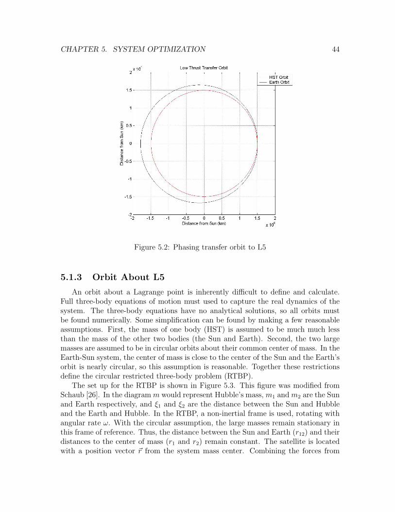
CHAPTER 5. SYSTEM OPTIMIZATION 44
Figure 5.2: Phasing transfer orbit to L5
5.1.3 Orbit About L5
An orbit about a Lagrange point is inherently difficult to define and calculate.Full three-body equations of motion must used to capture the real dynamics of thesystem. The three-body equations have no analytical solutions, so all orbits mustbe found numerically. Some simplification can be found by making a few reasonableassumptions. First, the mass of one body (HST) is assumed to be much much lessthan the mass of the other two bodies (the Sun and Earth). Second, the two largemasses are assumed to be in circular orbits about their common center of mass. In theEarth-Sun system, the center of mass is close to the center of the Sun and the Earth’sorbit is nearly circular, so this assumption is reasonable. Together these restrictionsdefine the circular restricted three-body problem (RTBP).
The set up for the RTBP is shown in Figure 5.3. This figure was modified fromSchaub [26]. In the diagram m would represent Hubble’s mass, m1 and m2 are the Sunand Earth respectively, and ξ1 and ξ2 are the distance between the Sun and Hubbleand the Earth and Hubble. In the RTBP, a non-inertial frame is used, rotating withangular rate ω. With the circular assumption, the large masses remain stationary inthis frame of reference. Thus, the distance between the Sun and Earth (r12) and theirdistances to the center of mass (r1 and r2) remain constant. The satellite is locatedwith a position vector ~r from the system mass center. Combining the forces from

CHAPTER 5. SYSTEM OPTIMIZATION 45
Figure 5.3: Set up for the restricted three-body problem (modified from Schaub [26])
both large masses and breaking the equations into x, y, and z components yields thefollowing equations of motion taken from Schaub [26]:
rx − 2ωry − ω2rx + G
(m1
ξ31
(rx − r1) +m2
ξ32
(rx − r2)
)= 0 (5.6)
ry + 2ωrx − ω2ry + G
(m1
ξ31
+m2
ξ32
)ry = 0 (5.7)
rz + G
(m1
ξ31
+m2
ξ32
)rz = 0 (5.8)
These equations of motion are numerically integrated using the end conditions fromthe transfer orbit as initial conditions. The orbit was followed for a period of 10years. The most difficult part of developing the mission geometry was finding aproper transfer orbit that would allow for a quasi-stable orbit about L5. Tweaking thetransfer orbit resulted in the L5 orbit pictured in Figure 5.4. This orbit is a pseudo-elliptical, quasi-stable orbit. The orbit is pictured relative to a stationary L5. Eachloop of the orbit lasts about 1 year; after 10 years the craft begins to leave the vicinityof L5. However, this trajectory requires no stationkeeping. But, solar radiationpressure and other-body perturbations are not involved in this calculation. Hubblewill have the ion engines and remaining fuel available to counteract any perturbationeffects.
5.1.4 Overall Mission Specifications
The mission geometry for the Hubble retrofit consists of three distinct parts:escape from Earth, transfer to L5, and orbit about L5. Both the Earth escape andthe transfer orbit require the use of the ion propulsion add-on module. Together the

CHAPTER 5. SYSTEM OPTIMIZATION 46
Figure 5.4: HST orbit relative to L5, in a rotating frame of view
two orbits require a ∆V of approximately 8030 m/s. The total time of transfer fromLEO to the L5 orbit is approximately 861 days (2.36 years). Using 5 ion drives withan Isp of 2740 s, this orbit scheme requires Hubble to carry 4200 kg of Xenon fuel.
5.1.5 Attitude Control
The Hubble Space Telescope was built with the most accurate pointing controlsystem ever. This system will be able to continue controlling the attitude of HSTafter the retrofit procedure. The retrofit module attached to the back of the telescopeis small enough compared to the size of Hubble that it will present no problems for theattitude control system. The software of the controller will need to be reprogrammedin order to account for new structural modes and moments of inertia, but that isbeyond the scope of this project. Aging hardware will also need to be replaced, inorder to insure a long operational lifetime. The six inertial rate gyroscopes are mostprone to failure, and all six will be replaced in the retrofit mission. The gyros weresupposed to replaced in Service Mission 4.
In its current Earth orbit, the Hubble uses its magnetic torques rods to performmomentum dumping maneuvers. Once HST reaches L5, it will no longer be able touse this method. At L5, the easiest external torque to use would be a solar radiation
CHAPTER 5. SYSTEM OPTIMIZATION 47
pressure effect. An external torque could be obtained by having independently actu-ated solar arrays. With one array full on into the Sun and on tilted perpendicular tothe Sun, a torque is created.
5.2 Propulsion
Ion propulsion is a form of electrostatic propulsion that works due to the ionizationof the propellant. The propellant gas is ionized through the use of direct electronbombardment or radio frequency fields to increase the temperature of the gas. Thegas is then accelerated through an electric field to produce the desired thrust. Thegas used to propel this type of engine is Ar (Argon), Xe (Xenon), or the vaporizedform of Hg (Mercury) or Cs (Cesium). The stored gas then enters the ionizationchamber to increase its temperature up to the thrust temperature. The gas passesthrough two acceleration grids which bombard it with positive ions from the powersource. Before reaching the nozzle the accelerated mass of ionized gas is then injectedwith electrons. Thrust is then obtained and the exhaust beam is electrically neutralbehind the engine nozzle.
Ion propulsion systems have many benefits over other conventional propulsionsystems. Increased system efficiency allows for a reduction in propellant mass of upto 90%. Lower propellent mass will reduce launch costs and allow for an increasein payload. Ion engines have extremely long operational lifetimes and high exhaustvelocities. The system obtains the highest degree of efficiency in converting electricpower into thrust.
5.2.1 Benefits of Using Ion Propulsion
Ion propulsion can provide a low thrust, constant acceleration mission. This lowacceleration provides great benefits, as it will not put unexpected stress on the existingHST, protecting its structure and delicate instruments. Since the ion propulsionsystem will provide low thrust and constant acceleration after a day of operation thecraft’s velocity will be accelerated by 30 feet per second. However, after a few monthsthe tiny force will increase the speed of the craft by around 10,000 miles per hour. Anion engine also pushes its exhaust faster than that of a chemical rocket using muchless propellant by a factor of ten. This form of propulsion can provide the safest andmost efficient means of performing this mission.
Secondly, an ion propulsion system would be able to provide a relatively low masssystem due to its increased efficiency. Research shows that ion propulsion systemshave no noted interference on broadcasting and telemetry operations, so this type ofsystem would have no effect on the HST’s communications system. Ion propulsion isalso less corrosive to satellite components than conventional propulsion systems andis safe to the environment. The scientific equipment and optics will perform betterwith this lack of contamination.

CHAPTER 5. SYSTEM OPTIMIZATION 48
For the HST Retrofit Mission, Xenon would be used as a propellant for the ionpropulsion system. Xenon has been found to offer the highest thrust of all the inert,non-reactive gases and is not corrosive or explosive. The Xenon will be released duringoperation into a chamber of ringed magnets, since the magnets enhance the efficiencyof the ionization process and keep the gas away from the chamber walls. Electronsthen are released from a cathode ray tube and collide with the Xenon atoms knockingthe electrons off these atoms, imparting a net positive charge turning them into ions.At the rear of the chamber a pair of electrically charged metal grids, one positive andone negative, generate an electrostatic pull on the ions. The ions are then yankedpast the grids at a speed of more than 65,000 miles per hour, right out the back ofthe engine into space. To prevent the Xenon atoms from being attracted back intothe engine chamber, an electrode at the rear of the engine emits free electrons thatmay rejoin the positive Xenon ions, rendering their charge neutral again.
5.2.2 Propulsion Analysis
A propulsion analysis is performed for the use of an ion engine for this mission (seeMatlab code in Appendix C). This analysis was based on a typical energy conversionefficiency, n equal to 91%. An approximation of HST’s total mass with retrofit addi-tion was calculated. The mass of the HST structure was calculated at about 25% ofthe total mass. A calculation of aPe, specific mass multiplied by the electrical poweroutput, was computed. The quantity aPe is proportional to the sum of the structuraland propellant mass. Using a selected mission ∆V , the engine’s exhaust velocity wascalculated using:
Ve =∆V
log aPe
Mtot+1
(5.9)
Using that exhaust velocity, Ve, the specific impulse, Isp, was calculated:
Isp =Ve
g(5.10)
The mass flow, m, for an ideal engine was then calculated based on the computedvalue of the specific impulse and the exhaust velocity:
m =
12· Isp−60
Isp
g · Isp
(5.11)
Next, the power required, P , for an ion engine was calculated:

CHAPTER 5. SYSTEM OPTIMIZATION 49
P =m · Ve · Isp · g
2 · n(5.12)
Finally, the thrust generated, T , for a particular engine was computed as:
T =2 · PVe
(5.13)
Based on the relationship:
P
T=
m · V 2e · 1
2
m · Ve
=Ve
2(5.14)
After iterating this process with orbital analysis models, the conclusion was reachedthat to perform this mission in a short period of time and escape the Earth’s sphereof influence quickly would require a mission ∆V of 8030 m/s. Using this value of∆V produced the following results for this type of ion engine being used on the HSTRetrofit Mission. The engine would have a specific impulse of 2740 seconds, an ex-haust velocity of 26,900 m/s, a power required of 4370 Watts, and would produce athrust of 0.537 N.
These results were typical of a high performance ion engine. However two problemswere encountered after seeing these results. A power requirement of 4370 Watts farexceed the power HST would be able to supply the engine and that a thrust of 0.537N would not allow for a timely mission and would lead to serious problems escapingthe Earth’s sphere of influence. After continuing the orbital analysis it was clear thata thrust of at least 2.0 N would be needed to perform a shorter transfer to L5. Sinceion propulsion was such a well suited propulsion system for this mission, other ionpropulsion solutions were examined. A working solution used five Xenon ion enginesfor the HST Retrofit Mission producing 2.69 N of thrust allowing the transfer to L5to be performed in adequate time.
The next and final problem that had to be solved with this propulsion system washow the HST could meet the power requirement for five engines at 22 kW if it couldnot even meet the requirements for one at 4.4 kW. Since there was only 5.4 kW avail-able from the HST’s solar panels another option was needed. The solution was to useRadioisotope Thermoelectric Generators, or RTGs. Radioisotope power generatorsconvert the heat (thermal energy) generated from the decay of radioisotopes into elec-tricity. The systems consist of Plutonium-238 (Pu-238) and other radioisotopes, oxidefuel and static electrical converter systems that use thermoelectric elements to con-vert the heat to electricity without moving parts. The major advantage of the static

CHAPTER 5. SYSTEM OPTIMIZATION 50
process is the simplicity and their high reliability. For one RTG using Strontium-90,the ratio of total power to system weight was 0.93 W/g. This RTG yielded a thermalpower output of 143 kW and a usable electric power output of 10 kW. The mass ofthis RTG is 154 kg and has a volume of 0.0512 m3. For the HST retrofit mission,RTGs could be used to supply power to the five engine propulsion system. A massof about 300 to 400 kg would have to be added to the HST, however the benefits ofusing an ion propulsion system far outweigh the disadvantages of using RTGs.
5.3 Environment
Environmental effects at L5 should be less noticeable than the effects Hubblecurrently experiences while orbiting Earth. Since the HST will be in constant contactwith the Sun, there will not be any thermal cycling from going in and out of eclipse.There is no evidence that any paranormal types or levels of radiation exist at thesesites, therefore no extra radiation protection needs to be added for the retrofit mission.
5.3.1 Thermal Shield
The added propulsion system and possible RTGs adds potentially more heatingto rear of Hubble than it was designed for. To account for this a thermal shield willbe placed between Hubble and the propulsion system. Several equations are used tocalculate the size of the heat shield. All of the equations from this section are fromReference [31]. The following equation is used to calculate the temperature on thepropulsion side of the shield:
Ts,1 =[
αq
Aσε
] 14
(5.15)
where q is the heat rate in W, from the RTGs and A is the surface area of the shieldin m2. The forward side of the shield is calculated to have the same temperature asa section of the Hubble would have with a layer of MLI insulating it. The followingequation is used:
Ts,2 =[αG
σε
] 14
(5.16)
where G is solar flux of 1400 W/m2. Next the thickness of the barrier had to bedetermined using the equation below:
t =kA(Ts,1 − Ts,2)
q(5.17)

CHAPTER 5. SYSTEM OPTIMIZATION 51
where t is the thickness in meters, and k is the thermal conductivity in W/mK. Theseequations are used to make a chart comparing aluminum, steel, and titanium. Table5.1 shows the surface temperatures of these materials and also the temperature ifcovered with MLI on both sides.
Table 5.1: Material properties and surface temperaturesMaterial a e k (W/mK) Ts1 K Ts2 KAluminum 0.379 0.0346 167 1180 721Steel 0.567 0.317 18 752 458Titanium 0.766 0.513 7.26 718 438MLI (outer) 0.12 0.3 n/a 517 315
Covering the shield with MLI brought down the surface temperatures thus allowingfor a smaller thickness of the shield. Table 5.2 shows a comparison of shield diametersand thickness.
Table 5.2: Shield diameters and thicknessMaterial D (m) t (m) D (m) t (m) D (m) t (m)Aluminum 6 3.3 3 0.83 2.4 0.53Steel 6 0.35 3 0.088 2.4 0.056Titanium 6 0.12 3 0.03 2.4 0.004
Another material option is Macor, a machinable ceramic made by Corning. Macorhas a modulus of elasticity of 66.9 GPa, similar to that of aluminum, a density of2550 kg/m3 which is comparable to aluminum, and a thermal conductivity of 1.46W/mK which is far less than any of the materials compared in the previous tables[4].
5.3.2 Solar Arrays
The new solar panels chosen for this mission are made of Gallium Arsenide (GaAs).The following equation is used to determine the maximum temperature that the arrayswould experience during the mission:
Tmax =
[(α− η)G
σ(εb + εt)
] 14
(5.18)
CHAPTER 5. SYSTEM OPTIMIZATION 52
where εb and εt is the emmitance of the top and bottom sides of the solar array, whichhave values of 0.825, α is the absorptance which has a value of 0.805, η is the solarefficiency with a value of 0.19, G is the solar flux of 1400 W/m2, and σ is the Stefan-Boltzman constant which is 5.67 x 10⁻⁸ W/m2 K4. The maximum temperature ofthe solar array is calculated to be 309 K. Gallium Arsenide has a melting point of1513 K, thus allowing it to be a suitable material for the mission.
5.3.3 Interior
No changes are required for the interior thermal systems of the Hubble SpaceTelescope. The only instrument that required a cooling system is NICMOS, whichcame with its own cryo-cooler, and is being replaced with the SBV. If an instrumenton Hubble needs a cooling system, it comes with its own. Hubble does have elec-tric heaters that can provide heat to any instrument bay if required by any of theinstruments.
5.3.4 Exterior
The exterior of the Hubble is coated with multi-layer insulation (MLI) and opticalsolar reflectors (OSR). It has been noticed that the areas covered by MLI were expe-riencing more heating than the areas covered with OSR. These areas of MLI were tobe replaced with OSR on Service Mission 4 (SM4). Service Mission 4 has since beencancelled. The HST Retrofit Mission will replace the MLI with OSR accordingly.The following equation is used to compare the two insulations: .
Tmax =[αG
σε
] 14
(5.19)
MLI has an absorptance and emmittance of 0.12 and 0.3, where the OSR has anabsorptance and emmittance of 0.04 and 0.83, giving the MLI a maximum tempera-ture of 315 K while giving OSR a maximum temperature of 185 K.
To compare the differences between the MLI insulation and the OSR, a thermalmodel of Hubble was created with ANSYS, a thermal modeling program. Figure 5.5shows the current Hubble configuration and Figure 5.6 shows the planned additionof OSR. These two models compare the different temperatures experienced by theHubble using different types of insulation. Figure 5.5 is a model of Hubble with theexisting MLI. The areas of the Hubble protected by the MLI reach temperatures ofapproximately 310K. The model in Figure 5.6 has replaced the MLI with OSR, whichallows for a temperature drop down to 185K.

CHAPTER 5. SYSTEM OPTIMIZATION 53
Figure 5.5: Current Hubble Thermal Configuration with only MLI
5.4 Power
Optimization of the retrofitted HST power system has been conducted through aseries of Matlab programs and research on the current power system. Factors such aspower loss, panel sizing, efficiencies, and battery selection are all considered duringoptimization.
A requirement of the retrofit mission is to remove HST from its current low Earthorbit. To do so, a propulsion system must be integrated into the existing systems.With the addition of a propulsion system, the power requirement will increase greatly.The best propulsion option lies in ion engines. The selected ion engines requireroughly 4.4 kW of power each. In order to meet the time restraints and avoid problemsescaping the Earth’s sphere of influence, 5 ion engines will be employed. The powerrequirement for the proposed propulsion system reaches 22 kW. The propulsion powerrequirement exceeds what can be supplied by solar arrays of the size currently used.
The power the solar arrays must provide during daylight to power the entire orbit(Psa) is calculated to determine the size of the solar arrays to meet power requirements(Asa). This calculation is done using the following equation:
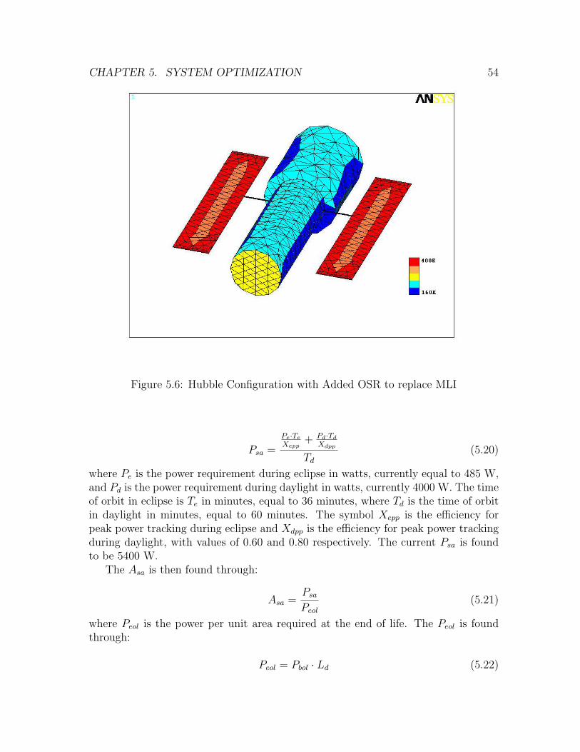
CHAPTER 5. SYSTEM OPTIMIZATION 54
Figure 5.6: Hubble Configuration with Added OSR to replace MLI
Psa =
Pe·Te
Xepp+ Pd·Td
Xdpp
Td
(5.20)
where Pe is the power requirement during eclipse in watts, currently equal to 485 W,and Pd is the power requirement during daylight in watts, currently 4000 W. The timeof orbit in eclipse is Te in minutes, equal to 36 minutes, where Td is the time of orbitin daylight in minutes, equal to 60 minutes. The symbol Xepp is the efficiency forpeak power tracking during eclipse and Xdpp is the efficiency for peak power trackingduring daylight, with values of 0.60 and 0.80 respectively. The current Psa is foundto be 5400 W.
The Asa is then found through:
Asa =Psa
Peol
(5.21)
where Peol is the power per unit area required at the end of life. The Peol is foundthrough:
Peol = Pbol · Ld (5.22)

CHAPTER 5. SYSTEM OPTIMIZATION 55
where Ld is the life degradation due to thermal cycling, micrometeoroids, plumeimpingement, material out gassing and radiation. The Ld is found to be 80% withthe following equation:
Ld = (1− degradation)Lsat (5.23)
where degradation, equal to 0.0275, is the typical GaAs cell degradation per year,and Lsat is the life of the satellite in years. At the end of our mission Lsat will be 10yrs. The power per unit area required at the beginning of life, Pbol, is determined bythe following equation:
Pbol = Po · Id · cosloss (5.24)
where cosloss is the cosine of the incidence angle between the array normal and sunvector in degrees (θo). In this case the worst-case sun angle of 30◦ was used. Theinherent degradation, Id, is equal to 0.77. The output power per unit area, Po, isfound from:
Po = η · 1358 (5.25)
where η is the production efficiency of GaAs solar cells (0.19).The Ld is found to be 80%, and Po is found to be 1220 W/m2, thus Pbol equals
170 W/m2. In turn, Peol equals 140 W/m2, and finally Asa is found currently to beroughly 40 m2.
With the addition of the ion engines, the power requirement increases by 22 kW,and would require an array with roughly the same size as the current arrays to powerone ion engine alone, and 6 times its current size to power the entire retrofittedHubble. Arrays of such a size would create problems in stability, and complicate theimplementation of the mission.
A solution to the power demand problem can be found with the use of RTGs.A particular RTG using Strontium-90 best fits the mission’s needs, as described inthe propulsion optimization section. A single Strontium-90 RTG produces 10 kW ofpower. Three Strontium-90 RTGs would meet the propulsion power requirement.
With the use of RTGs to power the propulsion system, it is assumed that the powerrequirement of all the other systems of the retrofitted HST will not exceed that ofcurrent HST. The retrofit mission will remove from HST instruments such as WFPC2,NICMOS with the NICMOS cryogen cooler, and COSTAR. The mission plans to addthe SBV, WFC3, and COS. With the removal of those three instruments, the additionof the three others, and the added propulsion system being powered independently,it is assumed that the power requirement will not increase.
The current Psa is 5400 Watts, and the Pbol for HST was roughly 170 Watts/m2.The Hubble’s mission was to end in 2010, and the Ld will be 80% by then. The powerrequired at the end of the mission per unit area (Peol) was found to be roughly 140Watts/m2. By 2020, the end of the mission, the Ld of the solar arrays would be 60%,
CHAPTER 5. SYSTEM OPTIMIZATION 56
resulting in a Peol equal to 100 Watts/m2. The Peol is short by almost 40 W/m2.Additional power must be supplied in order to carry out the mission until 2020.
To meet the power requirement at the end of life, many power sources could beapplied. Among the cheapest, and best for the mission, are solar arrays. The mission,once out of Earth’s orbit, will have constant exposure to the Sun, and solar arrayscould be employed to use such a limitless energy supply. Solar arrays have also alreadybeen proven more than satisfactory to meet the needs of the HST. The Peol deficitcould be met either by employing additional solar arrays, or replacing the currentarrays. Due to the age of the current arrays, and complexity of adding arrays to theHST, it is far more advisable to replace the arrays altogether.
The solar cell type that best suits the mission is a GaAs cell. The GaAs cellscan withstand temperatures well above those of the L5 environment. The solar ar-rays have already proven themselves on several space missions, including the currentHST mission. With the physical properties of GaAs solar arrays, and the power re-quirements, a proper array size can be calculated. With a 600 km initial orbit, 10year lifetime, 96 minute period, 36 minute eclipse, Psa equal to 5400 W, 30◦ anglebetween orbit plane and sun direction, degradation per year set at 0.02, and 0.04,and a varying η from 0.10 to 0.25, the following plot was made (Figure 5.7). Withknown production efficiency for GaAs solar cells equal to 0.19, and degradation peryear equal to 0.0275, the array area required to meet power requirements (Asa) isfound to be roughly 40 m2. Checking with the power model created in Matlab, theAsa is found to be 42.1 m2. The current arrays meet these requirements thereforearrays identical to the current arrays will make a satisfactory replacement. Two 8feet by 15 feet arrays are currently used, and meet the above criteria.
According to the Servicing Mission 4 (SM4) fact sheet [23], by NASA Goddard,the current batteries are over 13 yrs old, and due to natural degradation, shouldbe replaced. The SM4 fact sheet claims that the 6 original NiH2 batteries could bereplaced by newer versions of the same and meet the power requirements. If thepower loads are expected to not increase, then the original battery configuration willsuffice.
During Servicing Mission 3B (SM3B), the Power Control Unit (PCU) was replacedto meet the demands of the new arrays. By the time the mission is implemented,the PCU will have been in service for 8 years, and 18 years upon completion of theretrofit mission. The PCU needs to be replaced. The PCU installed on SM3B ismodeled for the new arrays, and is adequate for the mission requirements.
5.5 Communications
The communication system currently on the Hubble Space Telescope is composedof two S-Band Single Access Transmitters (SSAT) and two 1.2 meter high gain an-tennas. Hubble relays its data through the Tracking and Data Relay Satellite System(TDRSS) to communicate with Earth. The TDRSS satellites then send the data to

CHAPTER 5. SYSTEM OPTIMIZATION 57
Figure 5.7: Solar Array sizing. Array area as a function of production efficiency.
a ground station in White Sands, New Mexico, before being finally sent to the SpaceTelescope Operations Control Center (STOCC) in Greenbelt, Maryland. The SSATis capable of transmitting data at rates between 0.1 - 300 kb/sec [14].
The retrofitted Hubble will have to transmit from a distance of 150 million kmaway, the distance between Earth and Earth-Sun L5. The TDRSS satellites, whichare used for LEO satellite communications will not be an option for the new mission.The communications will have to go through the Deep Space Network.
5.5.1 Earth Communications
Since TDRSS is not an option for the new retrofit mission the Deep Space Net-work will be the new means of mission communication. The DSN will be used fordownlink/uplink of mission data, telemetry, and station keeping. The network hasthree main locations around the world, which are sited about 120◦ longitude fromeach other to give a transmitting satellite full Earth coverage. These DSN locationsare in California, Spain, and Australia.
The DSN transmits and receives at only two of the three bands being looked atfor the retrofit mission, the S-band and X-band. The Ku-band is not available for

CHAPTER 5. SYSTEM OPTIMIZATION 58
transmitting or receiving on the DSN, but due to improving satellite communications,it is safe to assume the Ku-band will be incorporated into the DSN by the missiontimeframe (2010). The frequency range for each band is listed in Table 5.3.
Table 5.3: Acceptable Frequency Band RangesFrequency Band Frequency (GHz)
S 2.5-2.54X 8.40-8.50Ku 12.5-12.75
The DSN also has three different antenna sizes to choose from: 26, 34, and 70meter dishes. As a failsafe in LEO, Hubble can use the DSN’s 26 meter dish to relaydata. Since there is a failsafe through DSN, relaying of the downlink data to STOCCin Greenbelt, Maryland is already in place. Selecting a DSN dish is the last item todetermine before a frequency band can be chosen. To improve data rate the 70 meterDSN dish is selected, giving the receiving antenna the highest possible gain.
5.5.2 Data Rate
Data rate is defined as the number of samples per second multiplied by the bits persample [31]. Data rate is the quantity of information per unit time transferred betweena spacecraft and the receiving antenna of another spacecraft or ground station. Thedata rate affects bandwidth choices, the sizes and shapes of the receiving antenna, andthe power required for the signal. The higher the data rate, the larger the antennaneeds to be to transmit for a given signal quality. The retrofit mission will have amaximum data rate of 650 Kbps to provide high quality images.
5.5.3 Retrofit Equipment
The retrofit mission will need new equipment to meet new requirements. Theuplink antenna will remain the same. The SSAT will be replaced with an X-bandtransmitter for the new mission due to a low data rate requirement for command andtelemetry. This low data rate is due to the low station keeping orbit around L5. Thedownlink antenna and transponder will need to be replaced for signal quality and tomaximize the data rate.
The downlink antenna signal quality depends on many factors. There are threemain losses to consider when dealing with signal quality: space loss, polarizationloss or transmission path loss, and transmitter line loss. Space loss is the loss dueto transmission distance and signal frequency. The transmission distance is a fixedparameter in the mission requirements and the frequency varies due to the selectedfrequency band. The two main frequency bands, which are being considered, are

CHAPTER 5. SYSTEM OPTIMIZATION 59
the X- and Ku-bands. The space loss then becomes a constant for each band. Thepolarization or transmission path loss comes from atmospheric and rain absorptionlosses, which are considered to be constant. The transmitter line loss is the lossbetween the transmitter and the transmitting antenna, which is also constant.
The next factor to consider is the antenna gain. All equations for this sectioncome from Reference [31]. The transmitting antenna gain for downlink utilizes thefollowing equation:
Gt =(π2 ·D2
t · η)
λ2(5.26)
where Dt is the antenna diameter in meters, η is the antenna efficiency, and λ is thewavelength of the frequency band being used. Antenna gain is usually expressed indB. The transmitting antenna gain gives you the EIRP, or Effective Isotropic RadiatedPower, given the following equation (in dB):
EIRP = Ptrans + Gt + Ll (5.27)
where the Ptrans is the transmitter output power, Gt is the transmitting antenna gain,and Ll is the transmitter line loss between the transmitter and the antenna.
To define the relationship between data rate, antenna size, propagation pathlength, and transmitter power, a link equation or link budget is used. The linkequation can be referred to as the ratio of received energy-per-bit to noise-density orEb
No. This ratio is used to determine the sizing of the communications system. The Eb
No
equation can be found below:
Eb
No
= EIRP + Ls + La + Gr + 228.6− 10 · log(Ts)− 10 · log(R) (5.28)
where Eb
No, Ls, La, and Gr are in dB, Ts is in K, and R is in bps. The symbol Ls is
the space loss term, La is the transmission path loss, Gr is the gain of the receivingantenna, Ts is the system noise temperature, and R is the data rate.
Before the link can be determined, a modulation and coding technique needsto be developed. Modulation is the process by which an input signal varies thecharacteristics of a radio frequency carrier [31]. Using a bit error rate (BER) of 10−5,
the Binary phase shift keying (BPSK) plus R− 12 Viterbi Decoding modulation was
selected based on excellent BER performance. The link equation for the selectedmodulation allows for a Eb
Noof 5 dB, which gives a BER of 10−5.

CHAPTER 5. SYSTEM OPTIMIZATION 60
Figure 5.8: Eb/No vs Antenna Diameter
Figure 5.8 shows the Eb
Noversus Antenna Diameter. A Eb
Noratio of 6 dB was chosen
to give the maximum data rate for selected modulation and still be within the signalquality limit of 5 to 10 dB. To size the antenna for the X-band transmitter and adata rate of 300 Kbps, a 3 m dish is needed. The Ku-band dish, given the samespecifications, will need a 2 m dish.
Figure 5.9 shows Eb
Noversus Data Rate. This figure compares the old antenna
diameter versus the new antenna diameter to determine the advantage of a new dish.From the data rate of 300 Kbps is where the values are taken. The X-band antennagives an Eb
Noratio of 6 dB at an antenna diameter of 3 meters. The current antenna
with a X-band transmitter gives an Eb
Noratio of -2 dB. The Ku-band antenna gives
an Eb
Noratio of 6 dB at an antenna diameter of 2 meters. The current antenna with a
Ku-band transmitter gives an Eb
Noof 2.5 dB.
Table 5.4 shows what antenna size will yield a data rate of 300 kbps for X-bandand Ku-band. Different antenna properties are also listed to measure the effectivenessof the antenna. The table also gives a wider range of acceptable data rate values foreach frequency band.

CHAPTER 5. SYSTEM OPTIMIZATION 61
Figure 5.9: Eb/No vs Data Rate
5.5.4 HST Computer and Data Storage
The original computer system on Hubble was designed specifically in the 1970’sfor space based operations. The computer is known as the Digital Fixed Point 2’scomplement 24-bit word Rockwell computer module (DF-224).
Due to system degradation, the DF-224 computer was upgraded and eventuallyreplaced. The DF-224 was first upgraded in 1993 during the first servicing missionby incorporating a new coprocessor based 80386 microchip. The computer was thenreplaced on the third servicing mission (SM3A) in December 1999. The replacementcomputer uses an Intel based 80486 microchip as its main processor. The new com-puter is faster by a factor of twenty and has more memory by a factor of six than theold one.
Hubble’s data storage devices were also designed in the 1970’s and used 3 reel-to-reel tape recorders. The tape recorders could store 1.2 gigabytes of data each. ASolid State Recorder (SSR) replaced one of the tape recorders when the coprocessorwas added to the DF-224. The SSR’s store data digitally and are capable of storing12 gigabytes of data each. A second tape drive was removed and replaced with anSSR during the same servicing mission that replaced the DF-224.
The retrofit mission will not need a new computer. Hubble’s current computerwill be able to run the new and old scientific instruments. The Space Based Visible

CHAPTER 5. SYSTEM OPTIMIZATION 62
Table 5.4: Antenna Characteristics for a given Band Frequency
Frequency Antenna Antenna EIRP Data Rate Eb/No C/No(GHz) Diameter (m) Gain (dBi) (dBW) Kbps dB dB-HzX-band
8.5 1.2 39 44.5 50 6 538.5 2 43.5 49 140 5.9 57.48.5 2.5 45.4 50.9 220 5.9 59.38.5 3 47 52.5 300 6.1 60.9
Ku-band12.5 1.2 42.4 47.9 110 5.9 56.312.5 2 46.8 52.3 300 6 60.712.5 2.5 48.7 54.3 450 6.1 62.712.5 3 50.3 55.9 650 6.1 64.3
(SBV) instrument can act independently of the computer. The SBV sensor has itsown processing computer to analyze the data it records. Because the computer doesnot need to be replaced, the retrofit mission will not encounter compatibility issueswith the older instruments. In addition, equipment will not have to be purchasedand built, which will reduce overall mission costs. However, the third reel-to-reeltape recorder should be replaced with a Solid State Recorder, so Hubble can storemore data onboard.
5.6 Mission Control
Information transmitted to and from the Hubble will have to be relayed betweenmany stations when HST is relocated to L5. Data transmitted from Hubble will gothrough the Deep Space Network’s 70 m dishes located at one of the three communi-cations facilities. From these stations, the data will be relayed to the flight controllersat the Goddard Space Flight Center in Greenbelt, Maryland. Finally, the data endsits journey at the Space Telescope Science Institute (STScI) in Baltimore, Mary-land where the data is turned into pictures and astronomical data. The path of thedata changes slightly, but the mission control will be able to remain the same. Theinformation for this section comes from Reference [21].
5.6.1 Deep Space Network
The Deep Space Network is the international network of radio antennas that willsupport the Hubble mission at L5. The network is part of the NASA Jet PropulsionLaboratory (JPL) and has three deep-space communications facilities that are placed
CHAPTER 5. SYSTEM OPTIMIZATION 63
approximately 120◦ longitude apart around the world. The facilities are: the Gold-stone Deep Space Communications Complex in Barstow, California, the complex inRobledo de Chavela 37 miles west of Madrid, Spain, and the Canberra Deep SpaceCommunications Complex, 25 miles southwest of Canberra, Australia. Each locationis in a mountainous, bowl-shapped terrain to reduce the radio frequency interfer-ence. These three facilities work together to keep constant observation of spacecraftas the Earth rotates. The DSN antennas are steerable, high-gain, parabolic reflectorantennas that will allow two-way communications to the Hubble.
5.6.2 Hubble Mission Control
At the “Hubble Mission Control” at Goddard Space Flight Center, a team “drives”the Hubble. Three operators, with dozens of engineers and scientists, comprise oneof four flight teams that work in shifts to operate the telescope 24 hours a day and7 days a week. These operators send over 100,000 instructions and receive over 10billion bits of scientific data each week.
The Hubble Mission Control at Goddard is formally the Space Telescope Oper-ations Control Center (STOCC). In the STOCC, the responsibilities are divided upbetween the scientists in five main rooms. These rooms are the Servicing MissionOperations Room (SMOR), the Mission Operations Room (MOR), the Mission Sup-port Room (MSR), the System Engineering and Evaluation Room (SEER), and theSTOCC “Back Room” positions.
Servicing Mission Operations Room (SMOR)
The Servicing Mission Operations Room is mainly used to support preparation,testing and simulations for Hubble’s servicing missions. The SMOR is also configuredto support the routine operations of the Hubble. The main division of work in thisroom is between the Mission Operations Manager (MOM), HST Systems, and HSTSystems Engineering Specialists.
The MOM has the controlling authority for all the STOCC operations. Theresponsibilities of the MOM position is to keep other positions informed of operationalstatus, and coordinates all “GO/NO GO” calls for the mission. The HST Systemsposition provides the systems engineering and analysis support. They are also theinterface with Johnson Space Center Payload Systems. The HST Systems EngineeringSpecialists are engineers that manage and provide analysis support for their individualsystems. These individual systems include: Data Management, Electrical PowerSystems, Instrumentation and Communication, Mechanical, Pointing Control, andOrbital Replacement Unit.

CHAPTER 5. SYSTEM OPTIMIZATION 64
Mission Operations Room (MOR)
The MOR is the room at the STOCC that controls and monitors Hubble flightoperations, including all engineering and science activities. This room also monitorsthe health and safety of the telescope. The positions include STOCC Operations, ShiftSupervisor, STOCC Operations Support Team, and the Ground System Manager.
The position of STOCC Operations provides an interface with the Johnson SpaceCenter and is in charge of coordinating all STOCC operations and mission scheduledevents and/or activities. The Shift Supervisor is the lead controller for the flightoperations team. As lead control, this position is in charge of issuing all commands tothe Hubble and is responsible for the configuration of the ground system. The STOCCOperations Support Team consists of many positions, including: CCS Support, DATAManagement/Communications/Power System Controller, Mission Support Analyst,Pointing Control/Science Instruments/Mechanisms Controller, and Sensor Analysisand Calibration Controller. This team is responsible for overall Hubble subsystemstatus. The Ground System Manager is the lead supervisor for all ground systemactivities.
Mission Support Room (MSR)
The MSR is important for day-to-day flight operations. This room will provide off-line mission planning functions and data processing to support both flight operationsand engineering activities. Data processing and mission analysis is also performedhere.
System Engineering and Evaluation Room (SEER)
The SEER is important for in-depth subsystem analysis. These engineers con-duct simulated subsystems tests, integrate new databases, and validate new groundsoftware and updates to flight software. The SEER can also be used as a backupoperations control room.
STOCC “Back Room” Positions
There are nine positions in this STOCC room, each having very specific func-tions. The positions include: Thermal Subsystems, Engineering Support System,Anomaly Response Manager, Servicing Mission Planning and Replanning Tool, Sim-ulation Team, Electronic Data Control Center, Data Operations Control, Network,and Video Imaging and Photographic Requirements.
The Thermal Subsystem is responsible for monitoring the temperatures of the tele-scope and any new replacement hardware. The Engineering Support System retrieveshistorical telemetry data of voltages, temperatures, currents, speeds, torques, switchvalues, and other values as needed. The Anomaly Response Manager resolves any

CHAPTER 5. SYSTEM OPTIMIZATION 65
problems that may arise during the Hubble’s mission. The Servicing Mission Plan-ning and Replanning Tool is responsible for preparing and revising a time-line andcommand plan for servicing the Hubble. The Simulation Team makes simulations forproblems and failures that may arise and presents them to the operations teams. TheElectronic Data Control Center provides the documentation for technical referenceand the dissemination of tactical data. The Data Operations Control is responsi-ble for the maintenance and operation of computer equipments, which processes theHubble’s data. The Network team ties together all the control computers. Finally,the Video Imagine and Photographic Requirements group maintains the electronicimaging system and database for the Hubble.
5.6.3 Service Mission Time
While Hubble is being serviced, the STOCC will become busy and additionalteams will be required. Since the Hubble will only be serviced once and then sent toa location where it cannot be serviced again, this increase in activity will only happenonce.
In the beginning of the mission, the STOCC commands the Hubble to prepare forSpace Shuttle rendezvous. Among these commands include closing the aperture doorand to stow the antennas. The shuttle crew can then install all of the new equipment.After the equipment is installed, the mission control team checks to make sure theequipment is functional and runs properly. Finally, the telescope is transferred tointernal power and the battery is charged. The Hubble can then be deployed and thepropulsion module can be engaged to send the telescope to L5.
5.6.4 Space Telescope Science Institute
The STScI is where the HST scientists are located. After Hubble data completesits journey, the STScI scientists calibrate, store, retrieve, and distribute the sciencedata. The STScI is also responsible for allocating observing time and providing thesoftware tools for data manipulation.
The Multimission Archive at Space Telescope (MAST) is the HST’s primaryarchive and distribution center for the data. There are over 20,000 targets withmore than 100,000 observations that are available from this archive. Another impor-tant archive is the Hubble Data Archive (HDA), which contains science data from allcompleted HST observations and calibration files. This archive has over 9.5 Terabytesof data, which totals more than 279,000 science exposures.
5.7 Structures
The HST structure will be upgraded in a few main areas. A new communicationsdish will be attached, an additional propulsion module will be attached to the rear

CHAPTER 5. SYSTEM OPTIMIZATION 66
of Hubble and solar arrays will be replaced. See Figure 5.10.
Figure 5.10: CAD Model of the Hubble with New Retrofit Components
5.7.1 Structural Evaluation
Upon launch the Hubble withstood very large loads caused by the accelerationof the Shuttle. The Shuttle accelerates at a value of no more than 29.4 m/s2. Thisacceleration means that the HST has withstood a large loading during launch.
F = m · a = 11000 · 29.4 ≥ 300, 000N (5.29)
The new propulsion system that has been chosen is a combination of five Ionthrusters. The combined thrusters will provide a max load of 2.69 N. This load is1/120,000 the amount of the initial load Hubble received upon launch. The Hubblewill receive no structural problems when the craft is accelerated by the ion thrusters.
When the HST is docked to the Shuttle for servicing, it attaches to the FSS(FlightSupport System). The FSS allows the HST to be rotated in any direction for servicing.The loads experienced during the service mission will be greater than the 2.69 Ncompressive loads that the module will place on the HST. Therefore The propulsionmodule will be attached to the back of the FSS docking plate.
It will be narrow and short enough to ride along with the FSS. See Figure 5.13After the servicing mission, the FSS will stay attached and be separated from the

CHAPTER 5. SYSTEM OPTIMIZATION 67
shuttle permanently with the module intact. This separation will be done by usingtwo explosive bolts to separate the FSS docking plate from the existing FSS structure.
5.7.2 Upgrades
Solar arrays will be upgraded, replacing the old arrays. Figure 5.11 shows the arrayto be replaced. A new communications dish will be added for sending information.This 3.0 m dish will replace one of the old dishes making it much larger. All existingstructures will be reused to support the replacement structures.
Figure 5.11: Solar Array Configuration
5.7.3 Propulsion Module
The new propulsion module will consist of three parts: the ion thrusters, theRTGs and the fuel tank. This module has been designed to fit within the FSS itself.It will be installed on the HST as the last step of the Spacewalks. This must be donebecause it is too large to be on the FSS while it is moving about, but while in itsupright position it will be able to house the FSS (Figure FSSplus).
Pressure Vessel Design
A tank must also be added to the retrofit structure for fuel storage. The propulsionsystem needs 4200 kg of Xenon to power the mission.
A Lincoln Composites Type IV hybrid fully wrapped plastic pressure vessel willfit the needs of this mission. The tank is spherical in shape. The tank has the ability
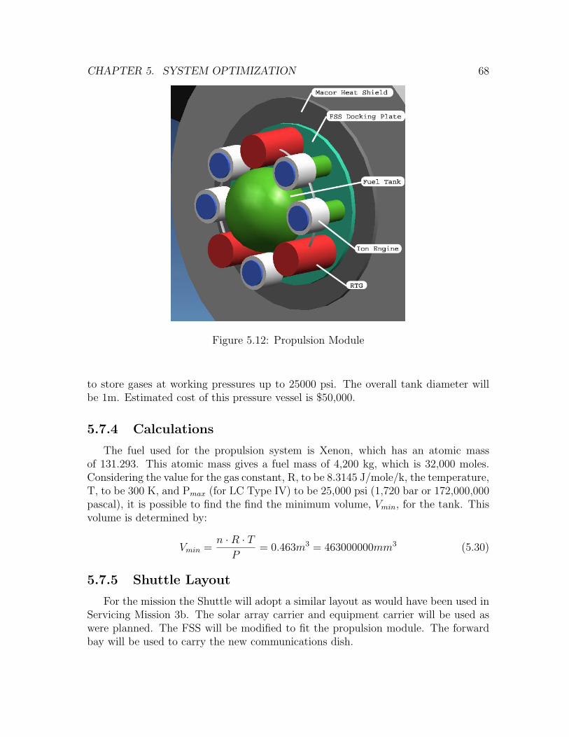
CHAPTER 5. SYSTEM OPTIMIZATION 68
Figure 5.12: Propulsion Module
to store gases at working pressures up to 25000 psi. The overall tank diameter willbe 1m. Estimated cost of this pressure vessel is $50,000.
5.7.4 Calculations
The fuel used for the propulsion system is Xenon, which has an atomic massof 131.293. This atomic mass gives a fuel mass of 4,200 kg, which is 32,000 moles.Considering the value for the gas constant, R, to be 8.3145 J/mole/k, the temperature,T, to be 300 K, and Pmax (for LC Type IV) to be 25,000 psi (1,720 bar or 172,000,000pascal), it is possible to find the find the minimum volume, Vmin, for the tank. Thisvolume is determined by:
Vmin =n ·R · T
P= 0.463m3 = 463000000mm3 (5.30)
5.7.5 Shuttle Layout
For the mission the Shuttle will adopt a similar layout as would have been used inServicing Mission 3b. The solar array carrier and equipment carrier will be used aswere planned. The FSS will be modified to fit the propulsion module. The forwardbay will be used to carry the new communications dish.
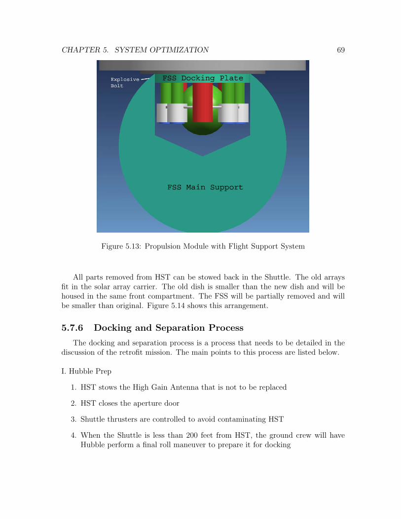
CHAPTER 5. SYSTEM OPTIMIZATION 69
Figure 5.13: Propulsion Module with Flight Support System
All parts removed from HST can be stowed back in the Shuttle. The old arraysfit in the solar array carrier. The old dish is smaller than the new dish and will behoused in the same front compartment. The FSS will be partially removed and willbe smaller than original. Figure 5.14 shows this arrangement.
5.7.6 Docking and Separation Process
The docking and separation process is a process that needs to be detailed in thediscussion of the retrofit mission. The main points to this process are listed below.
I. Hubble Prep
1. HST stows the High Gain Antenna that is not to be replaced
2. HST closes the aperture door
3. Shuttle thrusters are controlled to avoid contaminating HST
4. When the Shuttle is less than 200 feet from HST, the ground crew will haveHubble perform a final roll maneuver to prepare it for docking

CHAPTER 5. SYSTEM OPTIMIZATION 70
Figure 5.14: Shuttle Layout
5. HST solar arrays remain parallel to the optical axis
II. Capture
1. A Mission Specialist will operate the robotic arm to grapple HST
2. HST will then be maneuvered to the FSS (Flight Support System) to be latcheddown
3. The electrical umbilical is remotely engaged
4. Power is switched from HST to the Shuttle
III. Servicing
1. Replace batteries
2. Replace PCU
3. Replace transponders
4. Replace solar arrays
5. Replace antenna
CHAPTER 5. SYSTEM OPTIMIZATION 71
6. Replace rate gyroscopes
7. Replace solid state recorder
8. Remove NICMOS
9. Remove WFPC2
10. Remove COSTAR
11. Add OSR
12. Add SBV
13. Add COS
14. Add WFC3
IV. Release
1. Release the FSS pins with the propulsion module attached
2. When 200 ft from Shuttle Configuration and orbit modifications start
5.8 Instruments
For the retrofit mission, there will be three main instrument changes. The WFPC2will be replaced with the WFC3, COSTAR will be replaced with the COS, and NIC-MOS will be replaced with the Space Based Visible (SBV). The instruments WFC3and COS are already built and are mission capable. An SBV instrument has beendeveloped, but some alterations must be made to adapt it to the Hubble. The mainchange is that it will have to have its own corrective optics since COSTAR will beremoved.
The SBV sensor is a visible-band electro-optical camera that was first demon-strated successfully in 1997 (see Figure 5.15). It is currently a contributing sensorin the Space-Surveillance Network and would be even more useful attached to theHubble. The SBV has the ability to gather metric and photometric information ona variety of resident space objects. For this retrofit mission, it will concentrate onNEOs.
The on-orbit performance of the SBV sensor is shown visually in Figure 5.16. Theperformance allows a 22 cm in diameter specular sphere (with a reflectivity of 0.8)to be tracked at a range of 3000 km. This tracking uses high off-axis rejection opticsand can be used against a sunlight Earth-limb background at a tangent height of 100

CHAPTER 5. SYSTEM OPTIMIZATION 72
Figure 5.15: Space Based Visible [16]
km. Sensitive searches of large areas of the sky can be made using advanced staringfocal-plane arrays [16].
The greatest benefit to the SBV is that it has an onboard signal processor toreduce the volume of raw data. The processor can reduce the volume by as muchas a factor of a thousand (Figure 5.17). This reduction allows for more effectivedownloading of image data across narrow bandwidth telemetry links.
The SBV sensor has already demonstrated its ability with space-surveillance op-erations. Because of its success, the SBV has been incorporated into the Space-Surveillance Network as a Contributing Sensor. The sensor has already proven itselfequally in identified observations to the Ground-based Electro-Optical Deep-SpaceSurveillance (GEODSS), and with more accuracy. With the Hubble’s telescope beingused in conjunction with this sensor, the number of NEOs tracked can only increase.The Space Based Visible is an appropriate instrument for asteroid detection.
5.9 Summary
The system elements have been evaluated for feasibility, practicality, and havebeen optimized for application in the final HST Retrofit Mission. Each subsystemwas designed and optimized in equilibrium with all the other subsystems requirements.The final HST Retrofit Mission will incorporate these system designs to perform anoptimal mission which will be discussed in the following chapter.
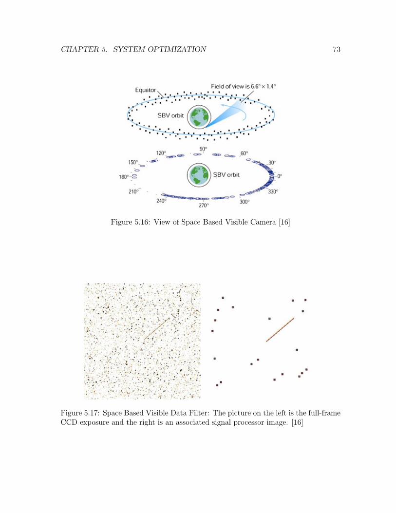
CHAPTER 5. SYSTEM OPTIMIZATION 73
Figure 5.16: View of Space Based Visible Camera [16]
Figure 5.17: Space Based Visible Data Filter: The picture on the left is the full-frameCCD exposure and the right is an associated signal processor image. [16]

Chapter 6
Final Configuration andConclusions
The primary objective of the Hubble Space Telescope Retrofit project has beento design future mission plans concerning the telescope itself. In order for the HSTto be used to its full potential for scientific discovery, the most optimal mission andsystem designs must be determined. Based upon the optimization and synthesis ofthe primary subsystems, with regard to the overall mission, one conclusive systemwill result. The final decision discusses the most efficient relationship between themission purpose and the individual subsystems of the HST. The chapter presents afully-designed mission purpose and operating system for future retrofit plans.
6.1 Mission Definition
The current mission of the Hubble Space Telescope will end in 2010, but possiblyas early 2008, after the completion of science operations. NASA is reviewing proposalsto extend the scientific life of the Hubble Space Telescope, as well as safely disposeof the Earth orbiting observatory at the end of its life in space.
The purpose of this project is to develop a follow-on mission for the Hubble.Subsystem modifications will be made to allow for a successful follow-on mission. Inaddition the Hubble must be removed from low-Earth orbit.
6.1.1 Objective
The project objective for a Hubble Space Telescope retrofit is to produce a missionand system design for a feasible follow-on mission. If found to be valuable and ofscientific gain, the mission could be adopted by NASA as an alternative to its currentde-orbit plans.
74

CHAPTER 6. FINAL CONFIGURATION AND CONCLUSIONS 75
6.1.2 Requirements and Constraints
The main requirement of this project is to design a mission and necessary hardwareto allow for successful completion of the mission. The following is a list of requirementsand constraints for the retrofit mission.
• Must be removed from LEO
• Must be compatible with current HST
• Must be implemented with a shuttle mission or autonomously
• Must have a minimum five year lifetime
6.2 Existing Hubble Components
As described in section 1.2, HST consists of several components that make theinner systems and outer structure. There are eight main instruments behind HST’sscientific missions. These instruments consist of the ACS, NICMOS, STIS, WFPC2,FGS, and COSTAR. The ACS is the newest of cameras with a wider field of viewand greater light sensitivity than the previous cameras. The NICMOS allows HST tosee through interstellar gas and dust, STIS acts like a prism for HST and separateslight into component wavelengths, and COSTAR corrects the spherical aberration inHST’s primary mirror. Also among the scientific instruments is the WFPC2, whichis responsible for almost all of the pictures known publicly, taken by HST. The FGSprovides data to the spacecraft’s targeting system and gathers data on the distanceand motion of stars. An aperture door is used to protect the optics, while the lightshield blocks out surrounding light.
Powering the scientific instruments, and all other components, are two 2700-wattGaAs solar arrays. The HST’s PCU, batteries and computer equipment are housed inthe electronic boxes. The computer support system modules house the systems vitalto controlling the HST. Data and information is relayed to ground stations throughTDRSS satellites from the communications antenna.
Three FGS lock onto two guide stars for orientation and positioning control, andensure a constant orientation. Also employed are two coarse Sun sensors, whichmeasure the orientation with respect to the Sun. The Magnetic Sensing Systemmeasures the Hubble’s orientation relative to the Earth’s magnetic field, the RateSensor Unit measures the attitude rate motion about its sensitive axis, and threeFixed-Head Star trackers are used to locate and track a specific star within their fieldof view. The actuator system of HST is used to adjust the orientation of the telescope.The actuator system is made up of reaction wheels and magnetic torquers. Fourreaction wheels accelerate or decelerate to exchange momentum with the spacecraft.The magnetic torquers are used primarily to manage reaction wheel speed.

CHAPTER 6. FINAL CONFIGURATION AND CONCLUSIONS 76
The outer structure is composed of stacked cylinders machined from aluminum,with the aperture door on top. The HST is shielded with blankets made of 15 layersof aluminized Kapton, with an outer layer of aluminized Teflon flexible optical solarreflector. An aperture door is used to protect the optics, while the light shield blocksout surrounding light. Also on the outer shell are two grapple fixtures, hand-holds,foot-holds, and a trunnion to lock the telescope into the shuttle cargo bay.
6.3 Hubble Retrofit Components
The Hubble Retrofit Mission requires replacements and additions outlined in thissection. The selected primary propulsion of the retrofit mission is the use of fiveion engines due to a ∆V requirement of 8030 m/s. These engines produce a specificimpulse of 2740 seconds, and produce a thrust of 0.537 N each. The engines will needa power source capable of supplying the 4.4 kW of power for each thruster, which hasa total power consumption of 22 kW. To handle the high power requirement, threeRTG’s will be attached to the propulsion retrofit module. The RTGs convert heatgenerated from the decay of radioisotopes into electricity without moving parts. TheStrontium-90 RTGs each produce 10 kW of usable electric power. Along with thepower requirement, ion engines accelerate an ionized gas to produce thrust. Xenongas is the fuel that best meets the retrofit mission requirements. A storage tank willneed to be attached to the propulsion module to hold the required amount of Xegas. The amount of Xe gas determined for the orbit transfer was calculated for threedistinct parts: escape from Earth, transfer to L5, and orbit about L5. Analyzingthese three parts of the orbit transfer, Hubble will have to carry 4200 kg of Xe gasfor the five ion engines.
The propulsion module will need a structurally sound attachment point. Thedocking pins located on the aft end of Hubble will be the perfect place to attachthe module. When Hubble is docked with the shuttle for servicing, the telescope isattached to these pins. Similar to launch loads, during servicing Hubble experiencesabout 2 N compressive loading.
Once in orbit around L5, Hubble will need to point at different locations to catalogNEOs and perform telescope tasks. Hubble uses six gyroscopes to measure angularrates. These gyroscopes will need to be replaced to give Hubble full attitude knowl-edge.
Due to the heat emitted from RTGs and the ion engines, Hubble will need a heatshield placed between the axial instrument bays and the propulsion module. Thematerial selected to provide a sufficient barrier is a machinable ceramic called Macor.Macor has a modulus of elasticity of 66.9 GPa, a density of 2550 kg/m3, and a thermalconductivity of 1.46 W/mK. These characteristics make Macor a very good materialfor the heat shield. Along with the heat shield the outer thermal barrier will needto be upgraded in some places. Optical solar reflectors will be placed in areas whereheating is exceeding the required limits.

CHAPTER 6. FINAL CONFIGURATION AND CONCLUSIONS 77
To perform the retrofit mission a power requirement of 5400 W is needed. Thesolar arrays currently on Hubble will be severely degraded by the time the retrofitmission takes place. Therefore, new Gallium Arsenide solar arrays will replace theexisting arrays. Using the GaAs cell type yields two solar arrays, sized 8 feet by 15feet to provide the required power output for Hubble. With a solar array change, thePower Control Unit will need to be replaced to meet the demands of the new arrays.Also, the 6 NiH2 batteries will be replaced due to degradation.
Hubble will need an upgraded communications system for the deep space mission.A three meter antenna with a Ku-band transmitter will provide the downlink com-munications. A maximum data rate of 650 kbps will be used to transmit data fromHubble to the corresponding ground stations. The uplink communications will keepthe 1.2 meter antenna and utilize an X-band transmitter due to minimal stationkeep-ing in the L5 orbit. Hubble will also need a new solid state recorder to allow for moreon-board data storage.
The retrofit mission will replace certain instruments to perform the new mission.The Cosmic Origins Spectrograph will replace COSTAR. The COS is the most sen-sitive ultraviolet spectrograph that would fly on Hubble. The WFC3 will replaceWFPC2. The WFC3 is a high-resolution/wide-field camera with continuous cov-erage of wavelengths from the ultraviolet to the near-infrared. The Near InfraredCamera/Multi-Object Spectrometer will be replaced by the Space Based Visible in-strument. The COS and WFC3 are already built and are mission capable. The SBVis the only instrument which needs to be adapted to work with Hubble. The sensor isa visible-band electro-optical camera that was first demonstrated successfully in 1997.The SBV has the ability to gather metric and photometric information on a varietyof resident space objects. This retrofit mission will use the sensor to concentrate onNear Earth Objects.
6.4 Mission Costs
The cost of the retrofit mission for the HST is comprised of main sections. Thereis the one-time cost of the components needed to retrofit Hubble, which will bedeveloped and readied for the launch in 2010. In addition, there is the one-time costof the shuttle launch, which is dependent on the mass of all the retrofit components.Finally, there are the ongoing mission operations costs.
A breakdown of the one-time cost of the components can be found in Table 6.1.The chart is broken down into subsystems, which each have their own components.These components have an associated mass and cost that contributes to the total costof the mission. A “∗” designation in the chart signifies this component was originallyintended for SM4. Therefore the cost does not need to be considered since it is built,tested, and ready to fly. The mass is important for these components to get the totallaunch mass.
For this retrofit mission, the space shuttle is being used. The shuttle launch is

CHAPTER 6. FINAL CONFIGURATION AND CONCLUSIONS 78
an expensive prospect. First, there is a base cost associated with the shuttle. Thisbase cost is found by dividing the total shuttle developmental costs by the amount ofprospective launches. This number averages to about $400 million [31]. In additionto this base cost, there is an associated cost of $16,400 per kg of payload launched[31]. Since there is a total of 6590 kg being launched, the payload costs are $108million. Considering an inflation factor of 1.131 (Reference [22]) for launch in 2010,the total launch costs then becomes $575 million.
The most expensive part of the mission is the operations costs. Operations costsencompass facilities, equipments, software, logistics, management, labor, and main-tenance. For one year of these operations, the Hubble costs $136 million (FY99$)[19]. With a considered inflation rate for each year, the total operations cost over tenyears of mission time will be $1.75 billion.
The retrofit mission for the Hubble is a massively expensive endeavor. The totalcosts for the mission, including one-time component costs, shuttle launch costs, andmission operations cost for ten years is $2.37 billion.
6.5 Mission Constraints and Optimization
The original proposal for this mission defined several needs and constraints essen-tial to its success. These items are presented in Chapter 1. The constraints to be metare a minimum mission lifetime of 5 years, and compatibility with the current HST.All components of the retrofit mission are designed to last for 10 years. The lifetimeshould be well over the required 5 years. The retrofit components for the mission areall either previously known to be compatible with the Hubble or specifically designedto fit with Hubble.
The needs defined for the mission were the addition of a propulsion module, theremoval of HST from low Earth orbit, an upgrade to the communications system,and the design of an overall feasible retrofit mission. A propulsion module consistingof 5 ion engines and three RTGs was designed to attached to the back of Hubble.An orbital scheme is provided to remove the Hubble from LEO and place it in anorbit about the Sun-Earth L5, which is far outside of LEO. A new communicationssystem for the Hubble was also designed. A larger antenna operating at a higherfrequency band is used to compensate for the huge distances over which Hubble mustcommunicate. However, the overall feasibility of the retrofit mission is somewhat inquestion. This topic will be discussed further in the next section.
Several design optimization parameters were presented in Chapter 2. These pa-rameters are listed in Table 2.1. The retrofit design attempts to satisfy these factorsin the best way. The scientific gain of the mission is maximized by allowing theHubble to continue its current studies, study the dynamics about L5, and study theSun’s magnetic field in addition to the search for NEOs. The lifetime was maximizedthrough the use of long duration parts. The weight and fuel usage of the retrofit wereminimized by using ion propulsion. A similar chemical system would have required on

CHAPTER 6. FINAL CONFIGURATION AND CONCLUSIONS 79
the order of 50,000 kg of fuel. The errors in Hubble’s attitude are already extremelysmall in its current configuration. Thermal effects are minimized by the replacementof Hubble’s layer of MLI with the much more effective optical solar reflectors. Powerusage was not minimized by the addition of multiple ion drives, but was accountedfor by the addition of the relatively light and efficient RTGs.
The design also attempted to minimize the cost of the retrofit mission. The launchcost is decreased significantly by the use of ion propulsion. Many of the componentsused in the retrofit are either already designed and built to fly on the Hubble, areavailable commercially off-the-shelf, or are already designed and just need to be scaledto fit HST. These facts will help keep down the design and construction costs. Themajor portion of the cost for this mission is the continued ground support for theHubble. This cost could be reduced if some of the science missions were no longerpursued, but this would of course decrease the value the mission as a whole.
The overall retrofit mission meets all of the design criteria and successfully ad-dresses all of the optimization parameters for the mission. On those terms, the retrofitdesign is a success. The overall feasibility of the mission will be discussed in the nextsection.
6.6 Overall Design Success
While the retrofit design successfully meets all of its criteria, its overall feasibility isquestionable. The retrofit procedure would be a huge manned undertaking, requiringa long preparation time and many hours of delicate spacewalk tasks. An autonomousretrofit robot would be just as difficult to design and deploy. The propulsion modulewould also be a complicated entity itself. Combining multiple ion thrusters into asingle craft has never been done before and could create unforeseen problems. How-ever, these problems are technical problems that could be overcome with iterationsof design.
The incorporation of several different missions creates other problems. Addingseparate science mission means that each individual mission will suffer for the goodof the whole. Using the Hubble Space Telescope for some of the proposed missionsis a definite overkill. Hubble is so massive that it is almost prohibitively expensiveto remove from Earth’s influence. Several smaller spacecrafts launched directly fromEarth could do a much better, cheaper job at individual missions. A smaller scopewith an SBV on it could produce a much more optimal asteroid hunting mission.The SBV could be sent cheaply and directly to a more effective observation location.The independent SBV craft could also be much more autonomous, operating as itwas originally designed to do, without the massive overhead and ground supportneeded by HST. An independent SBV would therefore be much cheaper to launchand operate, and would produce better results than the retrofitted HST.
An independent mission to L5 would also be more effective. A small, simplespacecraft is all that is needed to study the dynamics there. In fact, a design similar

CHAPTER 6. FINAL CONFIGURATION AND CONCLUSIONS 80
to or exactly like a previous mission could be used to save time and money. A goodmodel would be the ISEE-3 spacecraft. This extremely successful mission was thefirst to L1 and carried a suite of solar-studying instruments. Though not one of theoriginal project’s goals, it was decided the Hubble could investigate the Sun with itsmagnetometers. However, sending the Hubble with its magnetometer to study theSun is like sending an aircraft carrier to the North Pole to measure the temperaturewith a meat thermometer.
Based on the information in this report, it could be concluded that the Hubbleshould be left exactly where it is and allowed to continue its current missions. TheHubble has virtually revolutionized the field of astrophysics since its inception and itcontinues to make new discoveries nearly every day. As long as HST is still opera-tional, there will be a long line of astronomers waiting to point its instruments at aparticular spot in the sky. If NASA no longer wants to operate the Hubble, a privatefirm or nonprofit group could take over the telescope and run it more like a businessendeavor. The group could be in charge of its maintenance and ground control, andtherefore in charge of how the Hubble uses its time and capabilities.
In the long run, splitting the many goals of the retrofit mission into separateindividual missions would be more effective and economical. This separation woulddefeat the purpose of the retrofit, but not one of the missions would justify the costand difficulties in moving and modifying the telescope.
6.7 Summary
The Final Decision Chapter presents the chosen mission plans and operating sys-tem concerning the Hubble Space Telescope Retrofit project. The considerationstaken to arrive at such a decision have included: orbit options, attitude systems,thermal system designs, power maintenance, means of propulsion, networking commu-nication, system structures, and mission plans. Incorporating elements from previouschapters, the final decision has outlined an optimal retrofit mission design.

CHAPTER 6. FINAL CONFIGURATION AND CONCLUSIONS 81
Table 6.1: Cost Component Breakdown
Subsystem Cost Component Mass (kg) Cost (US$)ADCS Xenon Fuel 4200 $4,200,000
Gyroscopes∗ 33.1 ($8,000,000)
Thermal OSR 200 $35,000Propulsion/Telescope Barrier 228 $108,000
Power NiH2 Batteries 300 $3,000,0008’×15’ GaAs Solar Arrays 216 $19,000,000Power Unit Control 55 $2,000,000RTGs 153 $600,000
Propulsion Ion Engines 500 $2,000,000
Communications 3 m Antenna 30 $200,000Ku-band Transmitter/transponder 5 $1,500,000X-band Transponder 5 $1,000,000Solid State Recorder 12 $5,000,000Gimble/Structure 100 $100,000
Structures Fuel Tank 15 $50,000Brackets and Bolts 0.25 $300Heat Shield 0.50 $200
Science Instruments COS∗ 178 ($65,000,000)WFC3∗ 281 ($83,000,000)SBV 78 $11,000,000
TOTAL COST $50,000,000

Appendix A
Orbit Code
The code for orbit analysis was written in Matlab and performs three separate nu-merical integrations, one for each phase of the mission. The top-level file, HSTOver-drive.m, calls the driver file for each orbit phase in succession. The first programcalled is HEsim.m. This file simulates HST’s escape from Earth and calls rhsHE.m,a file that contains the two-body, continuous thrust orbit equations. The final statefrom HEsim.m is then saved and passed to Htsim.m. This program numerically inte-grates Hubble’s transfer orbit to L5, using the two-body, continuous thrust equationslocated the file rhsHT.m. The final state from Htsim.m is again saved and passed onto RTBPsim.m. This file integrates orbits using the full circular restricted three-bodyproblem equations of motion, which are contained in rhsRTBP.m. The final programcalled is HPM.m. This file takes all of the saved data from the three integrations andplots the results.
%Hubble Escape Simclear all
global mdot mu T rspi freeflagT0 = 0.537*5;%NIsp = 2739.7; %sm0 = 11000 +5*100 +3*153 + 100 + 4200; %kgr0 = 6378+569; %kmmuSun = 1.3271544e11;%km3/s2muEarth = 3.986004415e5;%%km3/s2rSE = 1.4959965e8;%kmmdot = T0/(Isp*9.81); %kg/smu = muEarth; %km3/s2v0 = sqrt(mu/r0);%Sphere of influence%http://www.go.ednet.ns.ca/~larry/orbits/gravasst/gravasst.htmlrspi = rSE*(muEarth/muSun)^(2/5);%km
82

APPENDIX A. ORBIT CODE 83
freeflag = 1;i0 = 28.5*pi/180;%initial inclination%ifin = 0;ifin = 23.5*pi/180;%anywhere 23.5 and under will line up
% with the ecliptic if the time is right
%a0 = fzero(’alpha0’,23*pi/180,[],i0,rspi/r0);a0 = 4.1024*pi/180;
T = T0*cos(a0);
x0 = [r0; 0; 0; v0/r0; m0];%tspan = [0 365*24*3600*2]; run too long to find HST leaves Earth’s sphere%of influence at t = 3.383351023663838e+007 sec%results run again only up til that timetspan = [0 3.760398348011308e+007];%sec, integration limitsopts = odeset(’RelTol’, (1e-3), ’AbsTol’, (1e-6));
[t, SatState] = ode45(’rhsHE’,tspan,x0,opts);
% x = SatState(:,1).*cos(SatState(:,3));% y = SatState(:,1).*sin(SatState(:,3));% plot(x,y,’k’);% axis equalEscapeState = [t, SatState]; save EscapeState EscapeState
**************************************************************
%Hubble Plot Machine%Plots the various states of Hubbleclear all%Escape Orbit% var EscapeState = [t, r, rdot, theta, thetadot, m]load(’EscapeState’) x = EscapeState(:,2).*cos(EscapeState(:,4)); y= EscapeState(:,2).*sin(EscapeState(:,4)); figure plot(x,y,’k’);muSun = 1.3271544e11;%km3/s2muEarth = 3.986004415e5;%%km3/s2rSE = 1.4959965e8;%kmrspi = rSE*(muEarth/muSun)^(2/5);%km sphere of influence of earthtc = 0:0.1:2.1*pi; xc = rspi*cos(tc); yc = rspi*sin(tc); hold onplot(xc,yc,’r’) axis equal axis square grid title(’Low ThrustEarth Escape Orbit’) xlabel(’Distance from Earth (km)’)ylabel(’Distance from Earth (km)’) legend(’HST Orbit’,’EarthSphere of Influence’)

APPENDIX A. ORBIT CODE 84
%Transfer Orbit% varTXState = [t, r, rdot, theta, thetadot, m]load(’TXState’) xt = TXState(:,2).*cos(TXState(:,4)); yt =TXState(:,2).*sin(TXState(:,4)); figure plot(xt,yt,’k’);rSE = 1.4959965e8;%kmte = 0:0.1:2.1*pi; xe = rSE*cos(te); ye = rSE*sin(te); hold onplot(xe,ye,’r’) axis equal axis square grid title(’Low ThrustTransfer Orbit’) xlabel(’Distance from Sun (km)’) ylabel(’Distancefrom Sun (km)’) legend(’HST Orbit’,’Earth Orbit’)
%L5 Orbit% var L5State = [t, rx, ry, rz, rxdot, rydot, rzdot]load(’L5State’) figure%%%% Rotating frame view, dist from L5 %%%%rSE = 1.4959965e8;%kmrSun = muEarth*rSE/(muSun-muEarth); plot(L5State(:,2)-(rSE/2 -rSun),L5State(:,3)-(-rSE/2*tan(pi/3)),’k’) hold on% plot(L5State(:,2),L5State(:,3))plot(L5State(1,2)-(rSE/2 -rSun),L5State(1,3)-(-rSE/2*tan(pi/3)),’rp’) grid title(’10 YearTrajectory Relative to L5 (in km)’) xlabel(’Distance from L5(km)’) ylabel(’Distance from L5 (km)’) legend(’L5 orbit’,’StartingPoint’,0)
**************************************************************
% HST super doulbe driver fileclear all% Hubble Earth escape simulationHEsim disp(’Escape Sim done\n’)% Hubble transfer to L5 simulationHTsim disp(’Transfer Sim done\n’)% Orbit about L5 simulationRTBPsim disp(’Three Body Sim done\n’)% Hubble Plot Machine!!!HPM me = EscapeState(end,end) - (11000 + 500 + 3*153 + 100) mt =TXState(end,end) - (11000 + 500 + 3*153 + 100)
**************************************************************

APPENDIX A. ORBIT CODE 85
%Hubble Tranfer Simclear all load(’EscapeState’) load(’L5State’)
global mu T1 T2 Isp T3T1 = 0.31;%N%T2 = -0.306;%NT2 = -0.3057;%NT3 = -0.18;%NIsp = 2739.7; %s
w = 2*pi/(365*24*3600);%rad/smuSun = 1.3271544e11;%km3/s2muEarth = 3.986004415e5;%%km3/s2rSE = 1.4959965e8;%kmrSun = muEarth*rSE/(muSun-muEarth); rEarth = rSE - rSun;
mu = muSun;% 2-bodty heliocentric
rSatf = [0.75226067651959; -1.30286368747225; 0]*1e8;%km sun at originvSatRelf = [-0.31861371754824; -0.18417566545398; 0];%km/s relative to L5
%Assumes Earth at [1;0] moving in [0;1] directionm0 = EscapeState(end,6);%kgrSat0 = EscapeState(end,2)*[1;0] + rSE*[1;0]; vSat0 =(EscapeState(end,3)^2 +(EscapeState(end,2)*EscapeState(end,5))^2)^(1/2)*[0;1] +(muEarth/rSE)^(1/2)*[1;0];
tspan = [0 365*24*3600*7/6]; opts = odeset(’RelTol’, (1e-6),’AbsTol’, (1e-9)); x0 = [norm(rSat0); EscapeState(end,3); 0;EscapeState(end,5)*EscapeState(end,2)/(rSE+EscapeState(end,2))+w;m0]; [t, SatState] = ode45(’rhsHT’,tspan,x0,opts);
% x = SatState(:,1).*cos(SatState(:,3));% y = SatState(:,1).*sin(SatState(:,3));% figure% plot(x,y,’k’);% rSE = 1.4959965e8;%km% te = 0:0.1:2.1*pi;% xe = rSE*cos(te);% ye = rSE*sin(te);% hold on% plot(xe,ye,’r’)

APPENDIX A. ORBIT CODE 86
% axis equalTXState = [t, SatState]; save TXState TXState% rSat0 = TXState(end,2)*[cos(TXState(end,4)); sin(TXState(end,4));0]
- rSE*[cos(pi/3);-sin(pi/3);0]% vSat0 = TXState(end,3)*[cos(TXState(end,4));sin(TXState(end,4));0] + (
TXState(end,2)*TXState(end,5) - TXState(end,2)*w)*[cos(pi/2-TXState(end,4));sin(pi/2-TXState(end,4));0]
**************************************************************
function [xdot] = rhsHE(t,x)
%State Vector: x = [r; rdot; theta; thetadot; m]
global mdot mu T rspi freeflag
x1dot = x(2); x3dot = x(4); x5dot = -mdot;
if x(1) > rspi & freeflagdisp(’I/"m free! Free! FREE!’);tfreeflag = 0;
end%assume Thrust is in tangential direction
x2dot = x(1)*x(4)^2 - mu/x(1)^2; x4dot = -2*x(2)*x(4)/x(1) +T/x(5)/x(1)/1000;
xdot = [x1dot; x2dot; x3dot; x4dot; x5dot];
**************************************************************
function [xdot] = rhsHT(t,x)
%State Vector: x = [r; rdot; theta; thetadot; m]
global mu T1 T2 Isp T3
x1dot = x(2); x3dot = x(4);
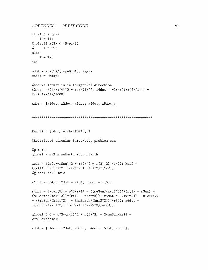
APPENDIX A. ORBIT CODE 87
if x(3) < (pi)T = T1;
% elseif x(3) < (5*pi/3)% T = T2;else
T = T2;end
mdot = abs(T)/(Isp*9.81); %kg/sx5dot = -mdot;
%assume Thrust is in tangential directionx2dot = x(1)*x(4)^2 - mu/x(1)^2; x4dot = -2*x(2)*x(4)/x(1) +T/x(5)/x(1)/1000;
xdot = [x1dot; x2dot; x3dot; x4dot; x5dot];
**************************************************************
function [rdot] = rhsRTBP(t,r)
%Restricted circular three-body problem sim
%paramsglobal w muSun muEarth rSun rEarth
ksi1 = ((r(1)-rSun)^2 + r(2)^2 + r(3)^2)^(1/2); ksi2 =((r(1)-rEarth)^2 + r(2)^2 + r(3)^2)^(1/2);%global ksi1 ksi2
r1dot = r(4); r2dot = r(5); r3dot = r(6);
r4dot = 2*w*r(5) + w^2*r(1) - ((muSun/(ksi1^3))*(r(1) - rSun) +(muEarth/(ksi2^3))*(r(1) - rEarth)); r5dot = -2*w*r(4) + w^2*r(2)- ((muSun/(ksi1^3)) + (muEarth/(ksi2^3)))*r(2); r6dot =-(muSun/(ksi1^3) + muEarth/(ksi2^3))*r(3);
global C C = w^2*(r(1)^2 + r(2)^2) + 2*muSun/ksi1 +2*muEarth/ksi2;
rdot = [r1dot; r2dot; r3dot; r4dot; r5dot; r6dot];

APPENDIX A. ORBIT CODE 88
**************************************************************
%Restricted circular three-body problem simclear all
global w muSun muEarth rSun rEarth
w = 2*pi/(365*24*3600);%rad/smuSun = 1.3271544e11;%km3/s2muEarth = 3.986004415e5;%%km3/s2rSE = 1.4959965e8;%kmrSun = muEarth*rSE/(muSun-muEarth); rEarth = rSE - rSun;
% rSat0 = [(rSE/2 - rSun)*(1.01); -rSE/2*tan(pi/3)*(.99); 0];% vSat0 = [0.3; 0.010; 0]; %best for 10 year r <~ 2.8e6 km% %vSat0 = [0.3; 0.0170; 0];% %vSat0 = [0.3; 0.0005; 0]; %best for 20 yr r <~ 5.8e6 km%Best Values:% rSat0 = [0.75226067651959; -1.30286368747225; 0]*1e8;% vSat0 = [-0.31861371754824; -0.18417566545398; 0];
load(’TXState’)rSat0 = R3(pi/3)*(TXState(end,2)*[cos(TXState(end,4)); sin(TXState(end,4));0]);
% - rSE*[cos(pi/3);-sin(pi/3);0]vSat0 = TXState(end,3)*[cos(TXState(end,4));sin(TXState(end,4));0]+ (TXState(end,2)*TXState(end,5) -TXState(end,2)*w)*[cos(pi/2-TXState(end,4));sin(pi/2-TXState(end,4));0]norm(rSat0) rSat0% global ksi1 ksi2% ksi1 = ((rSat0(1)-rSun)^2 + rSat0(2)^2 + rSat0(3)^2)^(1/2);% ksi2 = ((rSat0(1)-rEarth)^2 + rSat0(2)^2 + rSat0(3)^2)^(1/2);
tspan = [0 365*24*3600*10]; opts = odeset(’RelTol’, (1e-9),’AbsTol’, (1e-12)); [t, SatState] = ode45(’rhsRTBP’, tspan,[rSat0; vSat0], opts);
global C mean(C); std(C);
%PLotting done in HPM.m% figure% %%%% ROtating frame view, dist from L5 %%%%% plot(SatState(:,1)-(rSE/2 - rSun),SatState(:,2)-(-rSE/2*tan(pi/3)),’k’)% hold on% plot(SatState(1,1)-(rSE/2 - rSun),SatState(1,2)-(-rSE/2*tan(pi/3)),’r^’)

APPENDIX A. ORBIT CODE 89
% % plot(SatState(:,1),SatState(:,2),’k’)% grid% title(’10 Year Trajectory Relative to L5 (in km)’)%% figure% %%%% Non rotating view %%%% global posEarth0 vEarth% vEarth = sqrt(muSun/rEarth);% posEarth0 = [1,0]*rEarth;% tt = (0:100000:365*24*3600*1)’;% posE = ones(length(tt),2);% for jj = 1:length(tt)% posE(jj,:) = posEarth(tt(jj));% end% plot(posE(:,1),posE(:,2),’k’)% axis equal% hold on% satpos = zeros(size(SatState(:,1:3)));% for zz=1:length(t)% satpos(zz,:) = (R3(w*t(zz))*SatState(zz,1:3)’)’;% end% plot(satpos(:,1),satpos(:,2),’r’)% plot(satpos(1,1),satpos(1,2),’rx’)
L5State = [t, SatState]; save L5State L5State

Appendix B
Power Code
The power model.m Matlab code provided in this appendix ultimately computesthe area required by the solar arrays to meet power requirement, “Asa”, mass of solararrays, “Msa” and required batter capacity, “Cr”. With given values of initial alti-tude, radius of earth, power requirement during day and eclipse, length of respectiveperiods, efficiencies for peak power tracking, the Psa is found. With given degradationper year, inherent degradation, and production efficiencies of GaAs solar cells, alongwith the satellite life, the lifetime degradation, “Ld”, and the power per unit arearequired at beginning and end of life, “Pbol and “Peol” are found. In turn, the Asa
and Msa are found. With inputted number of batteries, battery efficiency, specificenergy density, depth of discharge and maximum bus voltage of NiH2 batteries, theCr is found in both watt-hours and amp-hours, “Cramphour”.
Gs=1358; %W/m^2 solar constant- total solar energy incident on a% unit area perpenicular to the suns rays at the mean% earth-sun distance outside the earth’s atmosphere
solarconst=1367; %W/m^2 at 1 AURe=6367; %kmH=600;%alt kma=Re+H; beta=acos(Re/a);theta0=(30*pi/180); % angle between orbit plane and sun directionalpha=asin(Re*tan(beta)/(a*cos(theta0)));timesunfrac=(pi+2*alpha)/(2*pi); %fraction of time in sunlight
%additional power required due to installation of instruments=?
Pe= 485; %power requirement during eclipse in wattsPd= 4000; %power requirement during daylight in wattsTe= 36 ; % length of period in eclipse (minutes) (orbiting earth currently)Td= 60 ; % length of period in daylight (minutes)(orbiting earth currently)Xepp= .60; % efficiency for peak power tracking during eclipse
90

APPENDIX B. POWER CODE 91
Xdpp= .80; % efficiency for peak power tracking during daylightXed= .65; %efficiency for direct energy transfer during eclipseXdd= .85; %efficiency for direct energy transfer during daylightPsa= ((Pe*Te/Xepp)+(Pd*Td/Xdpp))/Td; % power solar array must provide
% during daylight to power the entire orbit%Psa=2700*2; % for one array (so dont forget to mult by 2 later)
eta= .19; %production efficiency of gallium arsenide solar cellsId= .77; %inherent degredationcosloss= cos(30*pi/180); %incidence angle between array normal and sun vector
% (use worse case sun angle)
degradation= .0275; %typical gallium arsenide cell degradation per yearsatlife= 10; %satellite life (years) SA3 was performed march, 2002
% (will be 8yrs by 2010, 18 yrs by 2020))Ld= (1-degradation)^(satlife); %actual lifetime degradationPo=eta*1358; %output power/ unit areaPbol=Po*Id*cosloss; %power/unit area at beginning of lifePeol=Pbol*Ld;
Isa= 2; % current of solar arrays to meet requirement (amps)%Icell= ; %current output of a single cell%Npar= Isa/Icell; %number of cells in parallel (used to minimize shading effects%Vsa= ; % volatage of solar arrays to meet requirement%Vcell= ; % voltage output of a single cell%Psa=N*Pcell; %where N= number of cells in array, and Pcell=power produced
% by a single cell%Pcell=Psa/N;Asa= Psa/Peol; % solar array size to meet power requirement (m^2)Msa= 0.04*Psa; % mass of solar arrays (range from 14 to 47 W/kg)
%Pcell=Vcell*Icell; %%N=Psa/Pcell;%Nseries=Vsa/Vcell; % number of cells in series (used to achieve desired
% bus voltage)%these figures still unknown
Nb= 6 ; %number of batteriesetab= .9 ; %battery efficiencySED= 39 ; %specific energy density (35-43 for individual pressure vessel design)DOD=.60; % depth of discharge-%capacity used furing a single discharge cycle
% (40-60 for NiH2)busvolt=32.7; %max bus voltageCr=Pe*Te/(DOD*Nb*etab); %battery capacity in Watt hrsCramphr=Cr/busvolt; % battery capacity in amp hrs
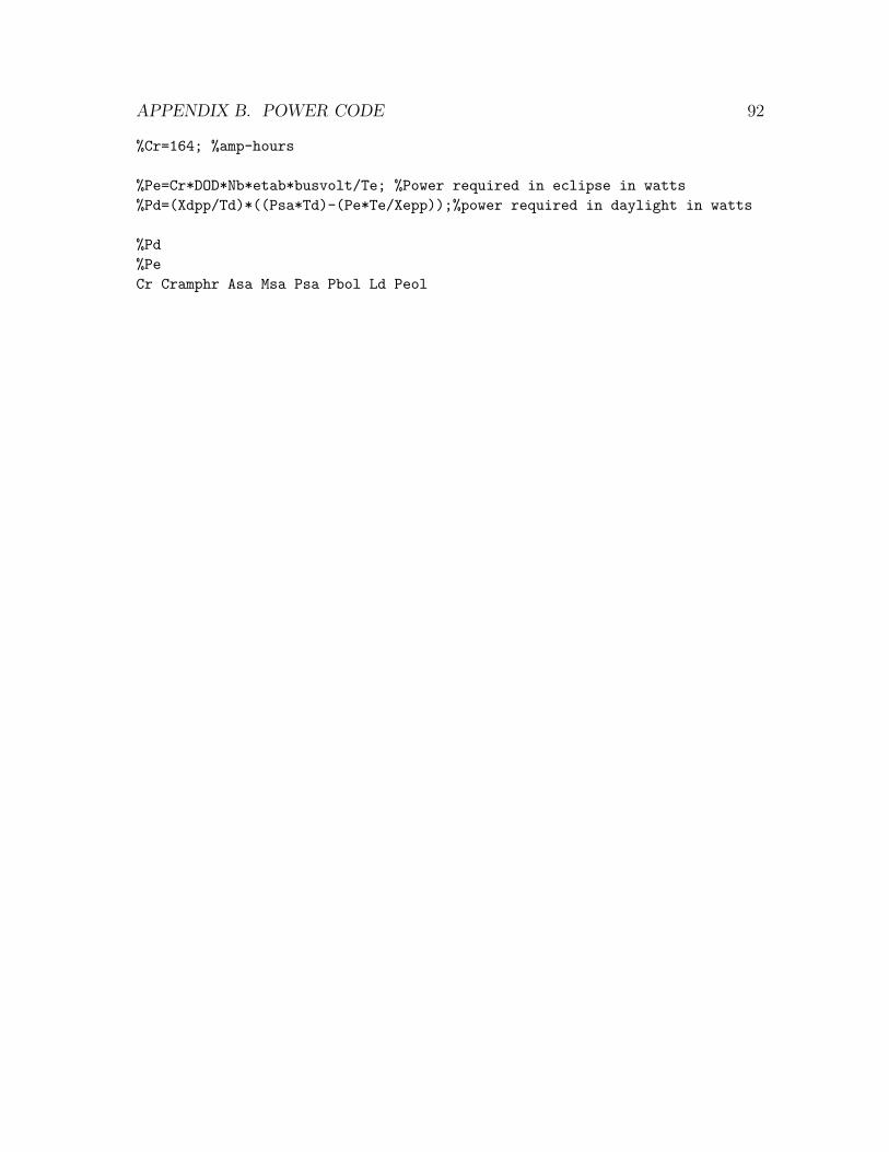
APPENDIX B. POWER CODE 92
%Cr=164; %amp-hours
%Pe=Cr*DOD*Nb*etab*busvolt/Te; %Power required in eclipse in watts%Pd=(Xdpp/Td)*((Psa*Td)-(Pe*Te/Xepp));%power required in daylight in watts
%Pd%PeCr Cramphr Asa Msa Psa Pbol Ld Peol

Appendix C
Propulsion Code
Propulsion.mThis program will calculate the Isp, exhaust velocity, power required, and
thrust generated for one ion engine given a delta V and other information about theretrofit addition. The mass of the batteries and xenon are a very close approximation.The mass of the actual retrofit addition structure is based on an educated estimate.RTG using Strontium 90, the total power system weight was 0.93 W/g. It was foundthat this type of RTG with a mass 154 kg each and a volume of 0.0512 m3 couldproduce 10 kW of electrical power based on an efficiency of 75%. This RTG seemsto be on the upper limit of technology at this time and using several could supportserious power needs.
Delta_V = input(’ Please input Delta_V (m/s): ’);
Mrs = input(’ Please input the mass of the retrofit additionstructure(kg): ’); Mp = input(’ Please input the mass of thebatteries and xenon (kg): ’);
% Some RTG information can be seen at the bottom of this code
Rt = input(’ Please input the number of RTGs used: ’); Rm =input(’ Please input the mass of one RTG (kg): ’);
g = 9.81; % Gravity (m/s)n = 0.91; % Energy conversion efficiency
(typical value)
Mr = Mrs + (Rt*Rm); % Total mass of the retrofitstructure (kg)
Mtot = 11300 + Mr; % Total mass (kg)
93

APPENDIX C. PROPULSION CODE 94
Ms = Mtot * .25; % HST structure (kg)
aPe = Mp + Ms + (Rt*Rm); % Specific mass * Electricalpower output
% proportional to the structuraland propellant mass
Ve = Delta_V ./ log(((aPe)./(Mtot))+1); % Exhaust velocity (m/s)Isp = Ve/g; % Calculating Isp (sec)mdot = (.5*((Isp-60)/Isp)) / (g*Isp); % Assume mass flow for ideal thrusterP = (mdot*Ve*Isp*g)/(2*n); % Power required for system (Watt)
Pp = 2*P;T = Pp/Ve; % Generated thrust per engine (N)
% based on (P/T)=(mdot*Ve^2*.5)/(mdot*Ve)= Ve/2
fprintf(’The Isp (s) of the ion engine is: %.1f\n ’, Isp);fprintf(’The Exhaust Velocity (m/s) of the ion engine is: %.1f\n ’, Ve);fprintf(’The power required (Watt) for the engine is: %.1f\n ’, P);fprintf(’The thrust generated (N) for the engine is: %.3f\n ’, T);
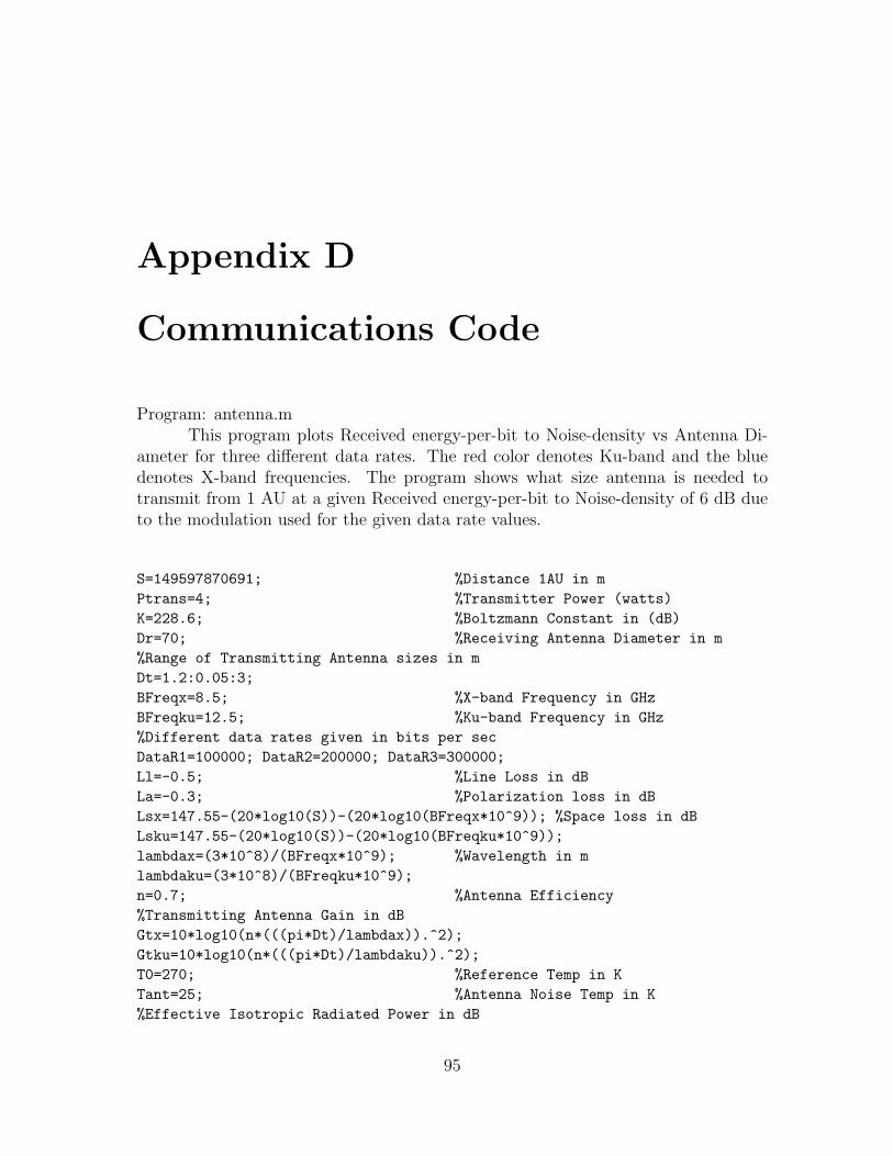
Appendix D
Communications Code
Program: antenna.mThis program plots Received energy-per-bit to Noise-density vs Antenna Di-
ameter for three different data rates. The red color denotes Ku-band and the bluedenotes X-band frequencies. The program shows what size antenna is needed totransmit from 1 AU at a given Received energy-per-bit to Noise-density of 6 dB dueto the modulation used for the given data rate values.
S=149597870691; %Distance 1AU in mPtrans=4; %Transmitter Power (watts)K=228.6; %Boltzmann Constant in (dB)Dr=70; %Receiving Antenna Diameter in m%Range of Transmitting Antenna sizes in mDt=1.2:0.05:3;BFreqx=8.5; %X-band Frequency in GHzBFreqku=12.5; %Ku-band Frequency in GHz%Different data rates given in bits per secDataR1=100000; DataR2=200000; DataR3=300000;Ll=-0.5; %Line Loss in dBLa=-0.3; %Polarization loss in dBLsx=147.55-(20*log10(S))-(20*log10(BFreqx*10^9)); %Space loss in dBLsku=147.55-(20*log10(S))-(20*log10(BFreqku*10^9));lambdax=(3*10^8)/(BFreqx*10^9); %Wavelength in mlambdaku=(3*10^8)/(BFreqku*10^9);n=0.7; %Antenna Efficiency%Transmitting Antenna Gain in dBGtx=10*log10(n*(((pi*Dt)/lambdax)).^2);Gtku=10*log10(n*(((pi*Dt)/lambdaku)).^2);T0=270; %Reference Temp in KTant=25; %Antenna Noise Temp in K%Effective Isotropic Radiated Power in dB
95

APPENDIX D. COMMUNICATIONS CODE 96
EIRPx=10*log10(Ptrans)+Ll+Gtx; EIRPku=10*log10(Ptrans)+Ll+Gtku;%Received Antenna Gain in dBGrx=-159.59+(20*log10(Dr))+(20*log10(BFreqx*10^9))+(10*log10(n));Grku=-159.59+(20*log10(Dr))+(20*log10(BFreqku*10^9))+(10*log10(n));%System Noise Temp in KTs=Tant+((T0*(1-0.89))/0.89)+((T0*(1.1-1))/0.89);
%Received energy-per-bit to Noise-density in dB for different data ratesEbNox1=EIRPx+La+Lsx+Grx+K-(10*log10(Ts))-(10*log10(DataR1));EbNoku1=EIRPku+La+Lsku+Grku+K-(10*log10(Ts))-(10*log10(DataR1));EbNox2=EIRPx+La+Lsx+Grx+K-(10*log10(Ts))-(10*log10(DataR2));EbNoku2=EIRPku+La+Lsku+Grku+K-(10*log10(Ts))-(10*log10(DataR2));EbNox3=EIRPx+La+Lsx+Grx+K-(10*log10(Ts))-(10*log10(DataR3));EbNoku3=EIRPku+La+Lsku+Grku+K-(10*log10(Ts))-(10*log10(DataR3));
figure semilogx(Dt,EbNox1) hold on semilogx(Dt,EbNoku1,’r’) holdon semilogx(Dt,EbNox2,’.’) hold on semilogx(Dt,EbNoku2,’r.’) holdon semilogx(Dt,EbNox3,’*’) hold on semilogx(Dt,EbNoku3,’r*’) holdon
grid xlabel(’Antenna Diameter (m)’); ylabel(’Receivedenergy-per-bit to Noise-density (dB)’); Title(’Receivedenergy-per-bit to Noise-density vs Antenna Diameter’);legend(’x-band (DR=100kbps)’,’ku-band (DR=100kbps)’,’x-band(DR=200kbps)’,’ku-band (DR=200kbps)’,’x-band(DR=300kbps)’,’ku-band (DR=300kbps)’);
**************************************************************
Program: datarate.mThis program plots Received energy-per-bit to Noise-density vs data rate for
two different antenna sizes. The red color denotes Ku-band and the blue denotesX-band frequencies. The program shows the difference between the actual antennasize HST has and the new antenna size that is needed to transmit from 1 AU. Thedata rate is determined by a predetermined Received energy-per-bit to Noise-densityvalue of 6 dB due to the modulation used.
S=149597870691; %Distance 1AU in mPtrans=4; %Transmitter Power (watts)K=228.6; %Boltzmann Constant in (dB)Dr=70; %Receiving Antenna Diameter in mDt1=1.2; %HST Existing Antenna Diameter in m%Transmitting Antenna Diameter in mDt=input(’Enter the diameter of the antenna in m: ’);

APPENDIX D. COMMUNICATIONS CODE 97
BFreqx=8.5; %X-band Frequency in GHzBFreqku=12.5; %Ku-band Frequency in GHz
%Range of data rates in bits per secDataR=100:100:1000000;Num=size(DataR); %Finds the size of the DataR matrixEnum=ones(1,Num(2)); %Creates a matrix of onesLl=-0.5; %Line Loss in dBLa=-0.3; %Polarization loss in dBLsx=147.55-(20*log10(S))-(20*log10(BFreqx*10^9)); %Space loss in dBLsku=147.55-(20*log10(S))-(20*log10(BFreqx*10^9));lambdax=(3*10^8)/(BFreqx*10^9); %Wavelength in mlambdaku=(3*10^8)/(BFreqku*10^9);n=0.7; %Antenna Efficiency
%Transmitting Antenna GainGtx1=10*log10(n*(((pi*Dt1)/lambdax)).^2);Gtku1=10*log10(n*(((pi*Dt1)/lambdaku)).^2);Gtx=10*log10(n*(((pi*Dt)/lambdax)).^2);Gtku=10*log10(n*(((pi*Dt)/lambdaku)).^2);T0=270; %Reference Temp in KTant=25; %Antenna Noise Temp in K
%Effective Isotropic Radiated Power in dBEIRPx1=10*log10(Ptrans)+Ll+Gtx1;EIRPku1=10*log10(Ptrans)+Ll+Gtku1; EIRPx=10*log10(Ptrans)+Ll+Gtx;EIRPku=10*log10(Ptrans)+Ll+Gtku;%Received Antenna Gain in dBGrx=-159.59+(20*log10(Dr))+(20*log10(BFreqx*10^9))+(10*log10(n));Grku=-159.59+(20*log10(Dr))+(20*log10(BFreqku*10^9))+(10*log10(n));%System Noise Temp in KTs=Tant+((T0*(1-0.89))/0.89)+((T0*(1.1-1))/0.89);
%Received energy/bit to Noise-density constant part of equationEx1=EIRPx1+Lsx+Grx+K-(10.*log10(Ts));Eku1=EIRPku1+Lsku+Grku+K-(10.*log10(Ts));Ex=EIRPx+Lsx+Grx+K-(10.*log10(Ts));Eku=EIRPku+Lsku+Grku+K-(10.*log10(Ts));DR1=(10.*log10(DataR)); %DataR matrix in dB
%Received energy/bit to Noise-density constant part * ones matrixENx1=Ex1*Enum; ENku1=Eku1*Enum; ENx=Ex*Enum; ENku=Eku*Enum;%Received energy-per-bit to Noise-density in dBEbNox1=ENx1-DR1; EbNoku1=ENku1-DR1; EbNox=ENx-DR1;EbNoku=ENku-DR1;

APPENDIX D. COMMUNICATIONS CODE 98
semilogx(DataR,EbNox1,’.’) hold on semilogx(DataR,EbNoku1,’r.’)hold on semilogx(DataR,EbNox) hold on semilogx(DataR,EbNoku,’r’)hold on
grid xlabel(’Data rate in bps’); ylabel(’Received energy-per-bitto Noise-density (dB)’); Title(’Received energy-per-bit toNoise-density vs Data rate’); legend(’x-band (Dt=1.2m)’,’ku-band(Dt=1.2m)’,’x-band (Dt=input)’,’ku-band (Dt=input)’);
**************************************************************
Program: SMADCOmm.mThis program calculates some of the link budget equations for a user defined
setup. The user inputs antenna size, the band frequency, and the data rate. Theprogram outputs antenna gain in dBi, EIRP in dBW, Received energy-per-bit toNoise-density in dB, and Carrier-to-Noise-density-ratio in dB-Hz.
S=149597870691; %Distance 1AU in mPtrans=4; %Transmitter Power (watts)K=228.6; %Boltzmann Constant in (dB)Dr=70; %Receiving Antenna Diameter in mDt=input(’Enter the transmitting antenna diameter in m: ’);BFreq=input(’Enter the Band frequency in GHz: ’);DataR=input(’Enter the datarate in bps: ’);Ll=-0.5; %Line Loss in dBLs=147.55-(20*log10(S))-(20*log10(BFreq*10^9)); %Space loss in dBLa=-0.3; %Polarization Loss in dBlambda=(3*10^8)/(BFreq*10^9); %Wavelength in mn=0.7; %Antenna EfficiencyGt=(n*(((pi*Dt)/lambda)).^2); %Transmitting Antenna Gain in dBGtdb=10*log10(Gt);T0=290; %Reference Temp in KTant=25; %Antenna Noise Temp in K%Effective Isotropic Radiated Power in dBEIRP=10*log10(Ptrans)+Ll+Gtdb;%Received Antenna Gain in dBGr=-159.59+(20*log10(Dr))+(20*log10(BFreq*10^9))+(10*log10(n));%System Noise Temp in KTs=Tant+((T0*(1-0.89))/0.89)+((T0*(1.1-1))/0.89);EbNo=EIRP+La+Ls+Gr+K-(10*log10(Ts))-(10*log10(DataR));CNo=EbNo+(10*log10(DataR));fprintf(’The Transmitting Antenna Gain in dB is: %.1f\n’,Gtdb);fprintf(’The EIRP in dB is: %.1f\n’,EIRP);

APPENDIX D. COMMUNICATIONS CODE 99
fprintf(’The Received energy-per-bit to Noise-density in dB is: %.1f\n’,EbNo);fprintf(’The Carrier-to-Noise-density-ratio in dB-Hz is: %.1f\n’,CNo);

Bibliography
[1] ABC. All Aboard The Interstellar Express. Internet document, 2003.http://en.wikipedia.org/wiki/Mini-magnetospheric plasma propulsion.
[2] European Space Agency. Ion Propulsion System to the Rescue. Internetdocument, 2003.http://www.esa.int/export/esaCP/ESANO40VMOC index 0.html.
[3] Bill Arnett. Asteroids. Internet document, 2003.http://seds.lpl.arizona.edu/nineplanets/nineplanets/asteroids.html.
[4] Inc. Automation Creations. Material Property Data. Internet document, 2004.www.matweb.com.
[5] AZoM.com. New Product: 10,000 psi Composite Hydrogen Fuel Tank.Internet document, 2002. http://www.azom.com/details.asp?ArticleID=1454.
[6] Roger R. Bate, Donald D. Mueller, and Jerry E. White. Fundamentals ofAstrodynamics. Dover, New York, 1971.
[7] R.A. Brown. The Role of Scientists in Developing Hubble Space Telescope.National Symposium and Workshop on Optical Platforms, 493:19–21, 1984.
[8] NASA Langley Research Center. The Hubble Space Telescope. Internetdocument, 2003.http://setas-www.larc.nasa.gov/HUBBLE/HARDWARE/hubble ORU.html.
[9] National Space Centre. Information Centre: Near Earth Objects. Internetdocument, 2004. http://www.nearearthobjects.co.uk/.
[10] Transportation Development Centre. Development of Safety Standards forCompressed Gas Vehicle Fuel Systems. Internet document, 2003.http://www.tc.gc.ca/tdc/publication/pdf/14000/14013e.pdf.
[11] David Darling. The Encyclopedia of Astrobiology, Astronomy, and Spaceflight.Internet document, 2003.http://www.angelfire.com/on2/daviddarling/index.html.
100
BIBLIOGRAPHY 101
[12] D. Fischer and H. Duerbeck. Hubble: A New Window to the Universe.Copernicus, New York, 1996.
[13] C.L. Foster, M.L. Tinker, G.S. Nurre, and W.A. Till. Solar-Array-InducedDisturbance of the Hubble Space Telescope Pointing System. Journal ofSpacecraft and Rockets, 32(4):634–644, 1995.
[14] Jeff Glass. S Band Return Signal Description. Internet document, 2004.http://nmsp.gsfc.nasa.gov/tdrss/srtn.html.
[15] J.C. Green. The Cosmic Origins Spectrograph. Internet Document, 2003.http://cos.colorado.edu/COS publications/cos spie3356Green.pdf.
[16] MIT Lincoln Laboratory. The Space Based Visible Program. Internetdocument, 2004. http://www.ll.mit.edu/ST/sbv/sbv table of contents.html.
[17] Pat L. Mangonon. The Principles of Materials Selection for EngineeringDesign. Prentice Hall, Upper Saddle River, New Jersey 07485, 1999.
[18] R.X. Meyer. Elements of Space Technology. Academic Press, San Diego, 1999.
[19] NASA. STS-103 Detail Page for Overview. Internet document, 1999.http://www.shuttlepresskit.com/STS-103/OVR102.htm.
[20] NASA. Hubble Space Telescope: Service Mission 3B Media Reference Guide.Internet Document, 2002.http://hubble.gsfc.nasa.gov/downloads/sm3b composite.pdf.
[21] NASA. The Hubble Space Telescope Project. Internet document, 2003.http://hubble.nasa.gov.
[22] NASA. Cost Estimating Website. Internet document, 2004.http://www.jsc.nasa.gov/bu2/inflation/nasa/inflateNASA.html.
[23] NASA. HST Fact Sheet. Internet document, 2004. http://hst-jwst-transition.hq.nasa.gov/hst-jwst/fact sheet SM4 manifest 21.pdf.
[24] University of Illinois. The Hybrid Rocket Motor. Internet document, 2003.http://stimpy.cen.uiuc.edu/soc/isds/hybrid/intro.htm.
[25] Seattle Print. Researcher’s nasa grant to float balloon theory on spacecraftpropulsion. Internet document, 2003.http://seattlepi.nwsource.com/local/nasa17.shtml.
[26] Hanspeter Schaub and John L. Junkins. Analytical Mechanics of SpaceSystems. AIAA, Reston, VA, 2003.

BIBLIOGRAPHY 102
[27] Jim F.H. Taylor. Radio Frequency for Galileo. Internet document, 1997.http://quest.arc.nasa.gov/galileo/Galileo-A/new/Radio frequency for Galileo.txt.
[28] H.F. Trucks. Space Telescope Maintenance and Refurbishment. NationalSymposium and Workshop on Optical Platforms, 493:93–104, 1984.
[29] Unknown. Magnetospheric Plasma Propulsion: Trapping the Energy of theSolar Wind. Journal of Geophysical Research, 105(A9), 2000.
[30] Joseph Wang. Spacecraft Propulsion. Class Notes - AOE 4174, Virginia Tech,2004.
[31] J.R. Wertz and W.J. Larson. Space Mission Analysis and Design, ThirdEdition. Microcosm Press, California, 1999.
[32] F.S. Wojtalik. Systems Engineering - Space Telescope Project. NationalSymposium and Workshop on Optical Platforms, 493:10–18, 1984.