Forced Liquidations, Fire Sales, and the Cost of Illiquidity

Richard R. Lindseyand

Andrew B. Weisman∗

January 14, 2015

“Vee try to tell them dat our problem was not a solfency problem but a likvitity problem, but they did notagree.” – A drunken senior staffer at the Central Bank of Iceland—As told in Boomerang, Lewis, (2011).

“JPMorgan Chase & Co. (JPM)’s announcement that an internal inquiry may show “intent” to mispricetrades in a unit that lost $5.8 billion may help a U.S. investigation while putting distance between manage-ment and any wrongdoers.‘Emails, voice tapes and other documents, supplemented by interviews’ were‘suggestive of trader intent not to mark positions where they believed they could execute,’ the bank said ina presentation yesterday as it reported net income fell 9 percent to $4.96 billion. ‘Traders may have beenseeking to avoid showing full amount of losses,’ the bank said, noting management had concerns about theintegrity of the prices used”—As reported by Leising and Hurtado in Bloomberg News, (2012).

1. Introduction

Institutional investors seeking diversification often build portfolios using collections of securities with widelyvarying characteristics. To help achieve diversification, investors generally use the common “currencies” ofreported return, volatility, and correlation to construct or optimize their portfolio. As a result, investors usingthis approach are often drawn to investment opportunities that appear to exhibit diversifying propertiessimply because of the limited price discovery associated with those investments. Such opportunities areoften relatively illiquid when compared to traditional investments like large cap stocks or sovereign debt,and investors frequently take for granted that they receive a “liquidity premium” that compensates themfairly for the lack of liquidity.1 A variety of approaches have been proposed to incorporate liquidity intothe portfolio optimization process: Seigel (2008), and Leibowitz and Bova (2009), develop methods forinstitutional investors to explicitly take liquidity into account when determining optimal asset weights; Ang,et al. (2011) characterize an investor’s optimal liquidity policy when there are frictions in the market; Lo,et al. (2003) add liquidity as an additional constraint in a mean–variance optimization; and Kinlaw, et al.(2013) incorporate liquidity as a shadow allocation to the portfolio.

The most common way to measure illiquidity in investments like hedge funds or private equity is serialcorrelation2 in the reported return series of the investment, because such serial correlation is frequentlyviewed as the result of price smoothing caused by exposure to less liquid securities or investments. Moresophisticated investors may adjust the return data by taking into consideration observed serial correlation inorder to decode the true volatility of the portfolio; they thereby correct both the volatility and the risk adjustedperformance of the investment (Scholes and Williams (1977); Geltner(1993); Getmansky, et al. (2004);

∗The authors would like to thank Mark Anson, Ashwin Alankar, Mark Baumgartner, Mark Kamstra, Mark Kritzman, Masao Matsuda,Fabio Savoldelli, Myron Scholes, and the participants of the 2014 Columbia MAFN Practitioner’s Seminar for useful comments anddiscussion. Errors remain our sole responsibility.

1Sparrow and Ilijanic (2010) quantify the value of liquidity in a trading context, and Amihud, et al. (2005) provide a literature surveyof the theoretical ways liquidity effects asset price.

2It went up (down) last period; so odds are it will go up (down) again this period—also referred to as autocorrelation. See e.g.Scholes and Williams (1977).

1

Bollen and Pool (2008); Anson (2010 and 2013)). Simply adjusting for serial correlation however fails tomeasure or capture the core risk and cost of illiquidity: forced liquidations and “fire sales”.

Forced liquidations typically occur when illiquid portfolios become overvalued relative to their true marketvalue (a relevant, timely valuation) and the reported valuation is no longer credible. Fire sales, or rapid salesof assets which depress prices, result when managers attempt to sell illiquid instruments or investmentsquickly. When these sales occur during significant adverse movements in the broader market with anassociated high demand for general liquidity, the price depression is exacerbated. Most importantly, forcedliquidations and fire sales often occur without warning, because they are precipitated by factors outside theinvestor’s control.

Many investors do not understand the true risk or cost of illiquidity until a forced liquidation or fire saleactually occurs—unfortunately, too late to help them. But by applying the barrier option pricing frameworkpresented in this paper to the expected return of an illiquid investment, investors can often know the prob-able cost of illiquidity in advance. The method described here allows investors to use a combination ofmarket data and experience combined in a consistent, analytically rigorous framework to derive a fair valueestimate of the cost of illiquidity.

2. Causes of Illiquidity

When it comes to liquidity, not all securities are created equal. Ask any experienced portfolio manager todescribe the agony associated with exiting a losing investment in the face of an illiquid, declining market—there is a qualitative difference and a real cost to exiting an illiquid portfolio compared with that of a liquidportfolio. Yet, in spite of the “lessons” learned during the global financial crisis of 2007–2008, many insti-tutional investments remain illiquid, and this illiquidity may be exacerbated during an extended low interestrate environment with low volatility, because asset managers are seeking higher returns.

One can think of the primary cause of illiquidity as a mismatch between the funding of the underlyinginvestment and the horizon over which the investment can be sold. Further, the greater the leverage em-ployed in the investment, the more likely it is that illiquidity will have a deleterious effect on the value ofthe investment in a declining market. Positions in exchange–traded securities can generally be sold veryquickly, although the seller of a large holding may experience significant price decline. In contrast, for aninvestment in real estate, even if the investor is willing to sell at a steep discount, it may still take a longtime to find a buyer. When investments are supported through the use of any form of short–term leverage3

or transactions that have embedded liquidity puts,4 there exists the potential for a funding mismatch and,therefore, illiquidity.

Additional factors can increase the illiquidity of any particular investment. Contractual terms like re-demption notice periods, lockups, or gates have liquidity costs that have been explored by Ang and Bollen(2010). They estimate that a three month redemption notice period, combined with a two year lockup forhedge funds, costs investors 1.5% of their initial investment and, if a gate is imposed, there is an additionalcost which can exceed 10.0%. Other factors—so called “network” factors—may not be as readily apparent.The use of common service providers (custodians, prime brokers, securities lending counterparties, or pric-ing providers); common investors such as fund–of–funds or large institutions (Battacharya, et al. (2013));or strategies which turn out to be correlated in unanticipated ways (Boyson, et al. (2010)) can create un-forseen illiquidity. In general, factors which cause implicit linkages may serve to create or increase illiquidityfor a particular investment or portfolio.

Investors in collective investment vehicles (such as hedge funds or private equity) are also subject to theactions of other investors in the same (or similar) portfolios. In some circumstances, if even a single largeinvestor decides to exit an investment, it can cause managers to sell assets to meet redemptions (Gennaioli,et al. (2012)). A high degree of leverage in the portfolio can also result in a rapid decrease in the value ofthe investment vehicle and thereby cause other investors to react. The economic advantage to being anearly redeemer if a portfolio or asset is under stress is well known (see e.g. Mitchell, et al. (2007) or Chen,

3Examples of short–term leverage may include margin borrowing (see e.g. Garleanu and Pedersen (2009) or Brunermeier andPedersen (2009)) or the use of futures, options, or swaps (see e.g. Office of Financial Research (2013)).

4Transactions which contain contractual obligations requiring liquidity upon demand, such as securities lending or repo transactions(see e.g. Keane (2013) or Office of Financial Research (2013)).

2

et al. (2010)), since slower investors end up holding shares of an increasingly less liquid portfolio (Manconi,et al. (2012)). For that reason, it has been shown that sophisticated investors withdraw much more quicklywhen there are questions associated with the liquidity of an investment (Schmidt, et al. (2013)).5

3. Liquidity and Reality

Consider first the nature of returns associated with trading and pricing a liquid security (or portfolio ofsecurities) versus that of an illiquid security. For liquid securities there exist virtually continuous, objective,and reliable price discovery; generally even large transactions do not suffer a significant increase in costupon liquidation. In contrast, illiquid securities, may trade only by appointment, at infrequent intervals,and without reliable, objective, public reporting.6 Sellers of illiquid securities cannot be certain about themarket value of their holdings, but sellers know (or should know) that a security’s sale price is likely tovary depending on the amount to be sold, the need to effect the transaction quickly, and price pressureassociated with other sellers in the market.7 All else equal, if a seller needs to sell a large amount in a shorttime then the price received can decline dramatically.

This lack of a liquid, transparent pricing mechanism tends to produce relatively predictable behavior bythe managers of less liquid portfolios. For example, it has been documented that portfolios of less liquidsecurities exhibit a high degree of positive serial correlation.8 In these cases, a significant proportion ofthe return in the current period can be statistically explained by the return in the prior period. This serialcorrelation is, of course, less likely to be the product of a wide–scale exploitable market anomaly, than theresult of the valuation practices of the managers of such less liquid portfolios (it may be useful to think ofprivate equity or certain hedge fund investments). Absent objective pricing, these portfolios tend to getmarked (priced) “conservatively”. In other words, prices are adjusted (and reported) by some proportion ofthe perceived difference between the point where they were marked during the prior period and the point atwhich they are believed to be “tradable” today. This approach does not necessarily imply nefarious behavioron the part of the manager,9 but can represent a simple Bayesian updating rule, using a partial adjustment oradaptive expectations approach, which is rational in that it minimizes the mean squared difference betweenthe estimated value and the market value (Quan and Quigley (1991)).

Over time, assuming markets move both up and down, the reported value (reported asset value or R)of the illiquid asset will be a relatively unbiased predictor of the true10 “tradable” value (true asset valueor N ).11 However, to the extent that a portfolio is “conservatively marked,” the reported returns will beautocorrelated, in other words, the current or observed return (rot ) will be determined, in part, by the priorperiod reported return (rot−1).

Why is this so? Consider Equation (1) which describes a typical “conservative” pricing strategy. Thereported return for the illiquid portfolio in the current period (rot ) is determined by adjusting the change inportfolio value by some proportion, λ (the reporting adjustment), of the difference between the prior periodreported value Rt−1 and Nt, the true, tradable value today.

rot =λ(Nt −Rt−1)

Rt−1(1)

We assume that the portfolio Nt, follows a discrete Brownian motion:

Nt −Nt−1 = Nt−1µ4t+Nt−1σεt√4t (2)

5Hill (2009) argues that options with long volatility exposures hedge some liquidity risk; Bhaduri, et al. (2007) apply this conceptin a number of hedging strategies; and Golts and Kritzman (2010) suggest that investors can protect for unscheduled capital calls bypurchasing liquidity options which pay the investor in those states of the world when such calls are likely.

6This is often the reason for low measured correlation and volatility.7This observation has been formalized by Acerbi and Scandolo (2008).8See e.g. Weisman (2003) or Getmansky, et al. (2004).9Nor does it preclude such behavior.

10“True” should be thought of in a generic sense as being some prudent central value for the price that would be obtained during agiven period if one wished to buy or sell the illiquid asset or portfolio.

11This paper uses the terms “asset” and “portfolio” interchangeably—one either has a single illiquid asset (e.g. an investment inprivate equity or a hedge fund) or a portfolio which contains illiquid assets (e.g. the even more illiquid portion of a hedge fund).

3

Here, the true value of the portfolio in the current period Nt is equal to its true value in the prior periodNt−1 multiplied by the trend rate of return (µ), and the one-period time step (4t), plus the assumed volatilityof the process (σ) multiplied by the product of εt (a standard normal random variable) and the square root ofthe one-period time step (

√4t). Thus, the change in value in any given period is the result of a combination

of a trend and a random shock.Substituting Equation (2) into Equation (1) and rearranging results in Equation (3), an expanded repre-

sentation of the observed rate of return over a period of length (4t):

rot =λ(Nt−1(1 + µ4t)−Rt−1) + λ(Nt−1σεt

√4t)

Rt−1(3)

Finally, taking the expectation of rot yields:12

E[rot ] =λ(Nt−1(1 +m4t)−Rt−1)

Rt−1(4)

As a consequence, the proportion of the expected value for period 4t explained by the actual value ofthe portfolio is λ. Recognize that although Nt and Rt have the potential for significant differences over time,(1 − λ) of the observed return will be explained by the prior period’s actual difference between Nt−1 andRt−1. The effect of this relationship is to induce first order serial correlation ρos(1) in the observed returnseries. This first order serial correlation is proportional to (1 − λ) even though the error term that helpsto drive the true return of the portfolio may be independent through time. For a quick and dirty estimateof the extent to which a portfolio manager is “conservatively marking” a portfolio (understating the changein its real value), one can simply calculate the first order serial correlation and subtract it from 1 to yieldan estimate of the proportion (λ) of the true change in the portfolio value that is being reported by themanager.13 As noted, even with a process that systematically under–adjusts for changes in valuation fromtime period to time period, the reported asset value may still be a relatively unbiased representation of thetrue value. Given that, the question becomes whether this misreporting is merely a benign understatementof the true volatility of the portfolio, which can be ignored, or whether it has a real cost to the investor.

4. The Barrier Option Framework

To answer this question we begin by examining the dynamics of how the two related processes (Nt and Rt)evolve over time. Figure (1) illustrates how Rt might track Nt over a randomly generated period of 60 timeintervals (for this simulation assume that µ = 0.05, σ = 0.25, and λ = 0.25). The “conservative” reportingprocess (in red) tends to “smooth” the valuation of the portfolio through time and, as expected, exhibits lessprice volatility than the actual, underlying series (in blue).

12The expectation is obtained by applying Ito’s lemma, where m = µ− σ2

2and µ is the arithmetic mean return.

13This relationship is explored in Appendix II.

4

Figure 1: Hypothetical Growth of $100

10 20 30 40 50 60100

120

140

160

180

200

220

Valu

e o

f $100

Period T

Actual Return Series

"Conservative" Return Series

Figure (2) depicts the individual period differences between Rt and Nt, where values above zero corre-spond to periods when the manager is over–valuing the portfolio relative to its true value. The manager’s“conservative” approach to valuing the portfolio results in periods of both significant under– and overvalua-tion. From a practical standpoint for an investor, undervaluation tends to be less important than overvalua-tion since having an investment which is worth more than its stated value is rarely harmful. Undervaluationis also rarely a concern for third parties providing financing to support the portfolio, since those parties areover–collateralized. But parties providing financing are usually quite interested in overvaluation. For exam-ple, a prime broker extending credit to finance the portfolio positions will want to ensure that the manager’sappraisal of the portfolio’s value doesn’t exceed some rational tradable value by more than a “reasonable”margin, since that value serves as collateral for the financing.

Figure 2: “Conservative” less Actual Returns

10 20 30 40 50 60−15

−10

−5

0

5

10

15

20

Perc

en

t O

vers

tate

d

Period T

Credibility Threshold

This reasonable margin of overvaluation may be referred to as the “credibility threshold” (L). Figure (2)

5

sets the threshold at 15.0%. When a manager exceeds the credibility threshold there is often a responseby interested parties; prime brokers tend to be take action promptly, but the response can be slower withlarger, more bureaucratic organizations like institutional investors, particularly when financial reporting isdelayed (as is the case for hedge funds). Regardless of where it arises, a breach of the credibility thresholdis likely to trigger forced behavior by the manager, in other words, the manager will be required to sell someor all of the illiquid portfolio in a relatively short time, typically in a descending or “thin” market. The singleperiod loss that occurs thus consists of two components. The first is a loss governed by (Rt − Nt), theextent to which the portfolio was overvalued. The second is a liquidation penalty (P ) associated with a firesale of the illiquid portfolio in a (typically) descending market. This liquidation penalty increases when theportfolio contains significant leverage since it is likely that more of the portfolio will need to be liquidated.Large, single period losses of this type are relatively common in financial markets and tend to be larger thanlosses estimated through the use of conventional and highly data–dependent methodologies such as valueat risk (VaR) or expected shortfall (CVaR). However, this paper suggests that these losses are somewhatpredictable, and that, by formalizing the basic structural dynamics described above, it is possible to developan objective framework for analyzing the cost of illiquidity.

When the credibility barrier is breached and a manager is required to liquidate positions as outlinedabove, one can model the associated cost as an up–and–in barrier option on the path of reported valuationof the portfolio.14 When the path of reported value is overvalued and exceeds the threshold (barrier), theoption “pays” (the “payment” is negative and represents a loss to the investor) the sum of two components,the amount by which the value of the portfolio was overstated and the additional loss associated with theforced liquidation. If the investor has a set of prior beliefs about: (a) the return and volatility characteristics ofthe portfolio (based on the observed mean, standard deviation, and serial correlation)15; (b) the conditionsthat will elicit a forced sale of the portfolio (i.e. a realistic estimate of the credibility threshold); and (c)the liquidation cost of being forced to sell a relatively illiquid portfolio during a stressful market period (anestimate of of the liquidation penalty), it is relatively straightforward to price the “option” using Monte Carlotechniques.16

First, simulate the “true” value of the portfolio using a discrete Brownian motion, a function of the ob-served volatility, and trend rate of return, and its associated estimated valuation lag, λ (which is based onone minus the observed first order serial correlation, (1− ρos(1))).

17 Then calculate the individual period dif-ferences between the two processes, and, when the difference exceeds the assumed credibility threshold,apply a payout equal to the difference between the two series at the time of the breach plus the assumedtransaction penalty associated with a forced liquidation. Do this 100,000 times, calculating the net presentvalue of whatever payout occurs for every one–year path, note that many paths will have no associatedpenalty. Finally, calculate the mean of the resulting payoffs (including the zero valued payoffs).

The option model is structured as a one year option so that the price translates as a “haircut” to thereported annualized rate of return associated with the investment. The price of the option is the de factoprice of the risk assumed by investing in the less liquid portfolio because the “conservatively–valued” port-folio may become significantly overvalued and thereby force a sudden, expensive liquidation. To arrive atthe liquidity–adjusted expected return of the portfolio, one simply subtracts the dollar value of the optionfrom the expected return of the portfolio (i.e. if the option is valued at $2.00 and the expected return of the

14We are not the first researchers to apply option theory to the issue of liquidity: Chaffe (1993)uses Black–Scholes option pricing tovalue illiquidity in private company valuations; Longstaff (1995) uses risk–neutral valuation to develop an upper bound on the value ofmarketability, and Golts and Kritzman (2010) use a cliquet option to hedge unexpected capital calls.

15Given that these are derived from returns reported by the manager, it is important to also use additional, independent sourcesto validate these parameters or the model may produce misleading results. See the discussion regarding the Bear Stearns fund inSection 6.

16Technically, the option is being given to the manager of the illiquid portfolio by the investor since the manager generally benefitsfrom holding illiquid assets through an asymmetric compensation structure (i.e. the manager shares gains on the upside, but does notshare investors’ losses on the downside). See Keane (2013) and Huang, et al. (2011).

17To generate paths for the “true” value of the portfolio, it is necessary to adjust the observed volatility for the serial correlation. Weuse the methodology developed by Geltner (1993):

σ =

√√√√( 1− ρo2s(1)

(1− ρos(1)

)2

)σ2o

where σ is the adjusted volatility, σo is the observed volatility, and ρos(1)

is the observed serial correlation.

6

investment is 10.00%, the adjusted return would be 8.00%).

5. An Example

To illustrate this approach, our base case is a portfolio with mean expected return, µ, of 6%; volatility,σ, of 12%; with a riskless rate in the market of 2%, all on an annualized basis.18 The one year barrieroption is valued on an initial $100 portfolio priced every week (52 times per year). When varying otherparameters, we fix λ (the reporting adjustment) at 25%, L (the credibility threshold) at 15%, and P (theliquidation penalty) at 25%.19 The evaluation of the option price is always based on 100,000 Monte Carlosimulations.20

Figure 3: Option Price as Function of λ and L

0.1

0.2

0.3

0.4

0.1

0.2

0.3

0.4

0

20

40

60

80

λ (R

eporting A

djustm

ent)

L (Credibility Threshold)

Op

tio

n P

rice (

$)

P=25% (Liquidation Penalty)

Figure (3) illustrates how the cost of the de facto option varies as a function of the reporting adjustmentλ and credibility threshold L when the liquidation penalty is held constant at 25%. As λ decreases, i.e. asserial correlation in the portfolio increases, the option value increases. Since we have used a one yearoption on a $100 portfolio, we can directly interpret the option value as an annual percentage cost to theinvestor for the illiquidity in the portfolio. For example, with a λ of 25%, a credibility threshold of 15%, and aliquidation penalty of 25% (our base case, approximately left of center in Figure (3)), the option has a valueof $15.54. This means that the investor should adjust the expected return for an investment in the portfolioby -15.54%. Since we have assumed an expected return of 6% for this portfolio, the illiquidity option thatthe investor is providing to the manager consumes all of the expected return from the investment; leavingan undesirable -9.54% liquidity–adjusted expected return.21 It important to recognize that for all credibilitythresholds below 20%, the value of the option is significant over a range of reporting adjustments (serialcorrelations).

Turning our attention to the influence of the credibility threshold, Figure (3) shows that as L increases(as the manager is given more latitude to overstate performance), the cost of the illiquidity option decreases.This result is expected since the likelihood that the credibility threshold will be breached goes down as thethreshold increases. Significantly, no one investor controls this threshold. While a given investor may be

18These are approximately market values at the time of writing.19We discuss the reasonableness of these values later in this Section.20Matlab code to price this option is included in Appendix I.21Note that this has not been adjusted for the cost associated with notification periods, lockups, or gates as described in Section 2.

7

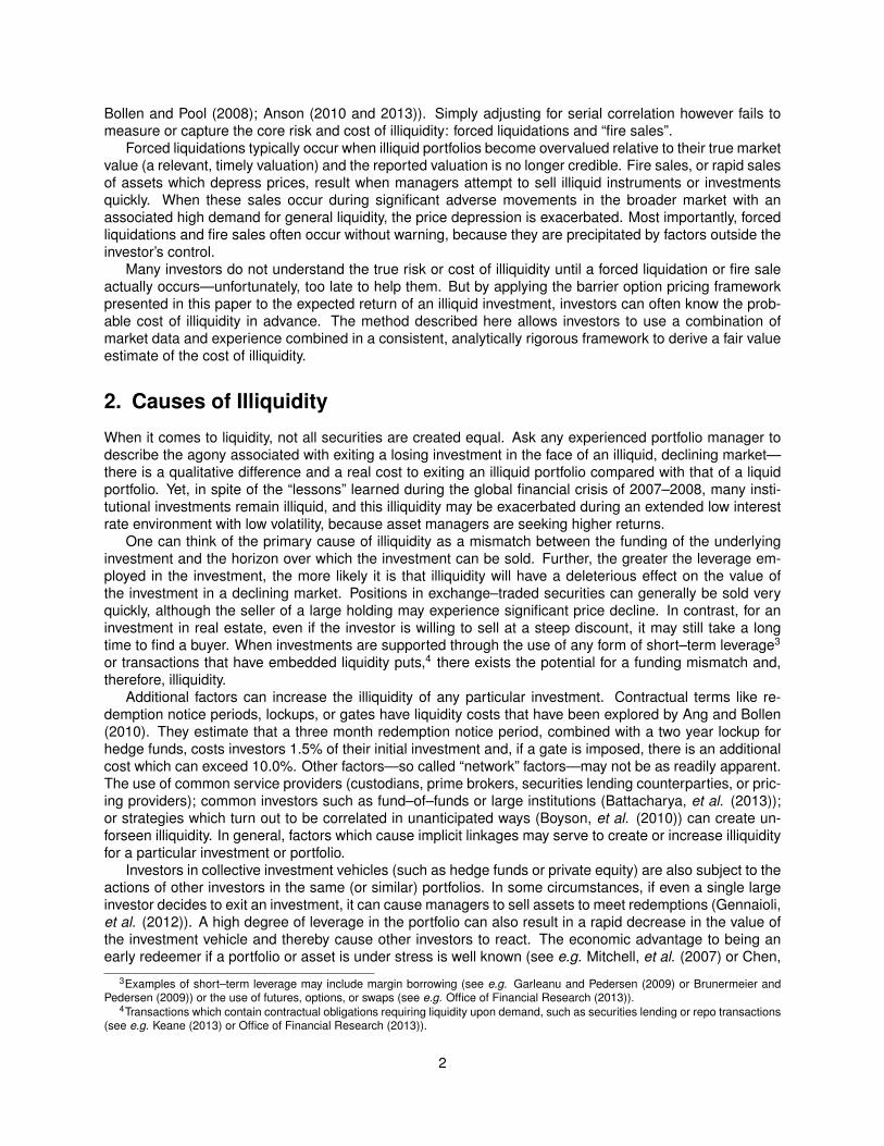
very lax (i.e. have a very high credibility threshold), it is the threshold of other investors or service providersthat “controls”—it is the credibility threshold of the market that matters.22

Figure (4) illustrates the relationship between the reporting adjustment and the liquidation penalty whenthe credibility threshold is constant at 15%. For higher reporting adjustment factors (lower serial corre-lations), the cost of the liquidity option is low. But for lower reporting adjustment factors (higher serialcorrelations), the cost of the liquidity option can increase dramatically. As might be expected, the cost of theoption is monotonically increasing in the size of the liquidation penalty, P . The steepness of the cost functionas the serial correlation increases underscores the cost of vanishing liquidity in a portfolio. As discussed inSection 2, when a portfolio is under stress, investors can be left with less and less liquid positions (resultingin higher and higher serial correlation). Figure (4) show that, in those cases, the cost of the illiquidity optioncan easily overwhelm the expected return of the portfolio.

Figure 4: Option Price as Function of λ and P

0.1

0.2

0.3

0.4

0.2

0.4

0.6

0.8

0

20

40

60

80

100

λ (Reportin

g Adjustment)

P (Liquidation Penalty)

Op

tio

n P

rice (

$)

L=15% (Credibility Threshold)

Figure (5) shows the relationship between the liquidation penalty and the credibility threshold when thereporting adjustment is held constant at 25%. As discussed above, when the credibility threshold is high(supervision is lax), the cost of the option is low. Otherwise, as the liquidation penalty increases, the costof the option also increases. For sensible ranges of the credibility threshold (5 to 15%) and relatively highserial correlations (e.g. 75%), the entire range of liquidation penalties results in significant cost associatedwith the illiquidity option. While the value of the illiquidity option diminishes with lower serial correlation, theassociated cost can still be important enough to investors to warrant estimation and consideration.

22More precisely, it is the lowest credibility threshold of any investor or third–party who has the ability to trigger a fire sale.

8

Figure 5: Option Price as Function of P and L

0.2

0.4

0.6

0.8

0.1

0.2

0.3

0.4

0

50

100

P (Liquidatio

n Penalty)

L (Credibility Threshold)

Op

tio

n P

rice (

$)

λ=0.25 (Reporting Adjustment)

It is also useful to consider the effect of the other parameters in the cost of the illiquidity option. When theriskless interest rate increases, the cost of the option goes down due to discounting—of course, the relativevalue of the investment should also be subject to the same discounting. When the number of pricing periods(i.e. the frequency at which the portfolio value is priced or marked) goes up, the cost of the option also goesdown, because the market can more quickly identify any overvaluation and therefore act upon any breachof the credibility threshold earlier. For portfolios with higher volatility, the cost of the option increases sincethere is a greater likelihood of overvaluation, and for portfolios with higher expected returns, the cost of theoption is lower since a greater expected return tends to offset the illiquidity option’s cost.

For the liquidation penalty, we have been assuming a base case value of 25%. Research by Ramadorai(2008), who analyzed transactions in the secondary market for hedge funds, found that, for those trans-actions involving fraud or collapse, the average discount to reported NAV was 49.6%, almost twice ourbase case value. As discussed earlier, as the liquidation penalty increases, the cost of the illiquidity optionincreases monotonically.

A few comments about this modeling approach. If one attempts to interpret the illiquidity option as theliquidity premium embedded in an investment, it appears to be much too high (approximately 15% in ourbase case). This is because the option approach used here does not price the liquidity premium investorsusually think of, but rather represents the cost associated with the price smoothing of an illiquid investmentwhich, when combined with a “triggering event”, results in an abrupt sale into a deteriorating market. Thesize of the illiquidity option is a function of the magnitude of manager mispricing and the cost of liquidating atan unfavorable price. The higher the degree of leverage employed in the underlying investment, the largerthe cost associated with any liquidation in the event of a fire sale. Clearly, actions taken by the manager canmitigate the value of the illiquidity option. For example, the manager could vary the reporting adjustment (λ)dynamically rather than using the static approach modeled here.23 This would allow the manager to controlthe degree of over– or under–valuation associated with the investment. In practice, we would expect thatmanagers would utilize such an approach. A manager could also liquidate a portion of the portfolio as thecredibility threshold is approached. However to modify behavior as the barrier is approached, the managerwould need a well–formed expectation about the level of the credibility threshold, which may be difficult toobtain since the barrier is not pre–established and is set by actors outside the manager’s control. In addition,the incentives to cheat may increase as the barrier is approached. Many managers get into trouble whenthey make the decision to hide bad results in an attempt limit the scope for investor withdrawals. Theyoften hope that the market will turn and bail them out of the situation. But most managers lack the flexibility

23This type of dynamic or state–dependent choice could theoretically be embedded in an general equilibrium setting.

9

to alter their book. Attempting to institute a portfolio insurance strategy or to sell off part of the book willexacerbate the situation because the positions will now have an accurate mark. Managers and investorscan generally live with a bit of variation around the “true” value of an illiquid investment, but if a managersdecides that the credibility threshold is close, trying to modify holdings or positions may actually trigger afire sale. Nonetheless, since we are not modeling an environment where the manager is making dynamicresponses, we believe that the option value represents an upper bound on the cost of illiquidity.

Finally, turning to the assumptions associated with expected returns and volatility, JP Morgan AssetManagement (2012), projects hedge fund expected returns in the range of 5 to 7% per year, with volatilitiesin the range of 7 to 13% per year—consistent with the assumptions of our base case. Importantly, JPMorgan estimates the expected returns for private equity at about 9% with a volatility of 34.25%. Sincevolatility serves only to increase the cost of the illiquidity option, only a high expected return (with reasonablelevels for the other parameters) can serve to offset the cost of illiquidity in the portfolio. One could questionwhether middle, single digit returns are truly sufficient for investors to bear the cost of illiquidity that manyhedge fund and private equity portfolios contain.

6. Pricing Liquidity in Alternative Investments

We are now in a position to consider several real world applications of the model and the implications forinvestors in less liquid portfolios. We begin by considering five well known hedge fund indices constructedby HFRI: (a) fixed income–convertible arbitrage, (b) distressed/restructuring, (c) multi–strategy, (d) fixedincome–corporate, and (e) emerging markets Russia/Eastern Europe. Table 1 contains estimates for thefirst order serial correlation from the inception of each index, along with the reporting adjustment whichwould be implied in each case. Note that the values shown represent index level estimates, so it is reason-able to assume that there could be a significant degree of variability in the underlying funds which constitutethe indices. As shown in Table 1, mean index serial correlations for most of these strategies lie in the 50to 60% range, implying an adjustment factor less than 0.50, i.e. where managers, on average, reflectless than 50% of the true period–to–period change in the value of their portfolios. Depending on an in-vestor’s assumptions concerning the liquidation penalty and the market credibility threshold, and estimatesof the expected return and volatility, the adjustment to observed returns (based on the cost of the illiquidityoption) could be quite significant. We would expect, however, for indices constructed with a large number ofunderlying funds that at the index or composite level, the over– and under–valuation of various managerswould be “diversified” away24 and that the liquidity option on an index should therefore be zero or close tozero. In fact, for the first four indices in Table 1, that is exactly what we find—the estimated option value iszero in each case. However, the Russia/Eastern Europe emerging market index, which reflects the lowestserial correlation in Table 1, has a monthly reported mean of 1.44% (17.30% annualized) and a monthlyreported standard deviation of 7.69% (26.64% annualized). The liquidity option is priced25 at 13.52, whichreduces the seemingly large 17.30% return to only 3.78% per year, and demonstrates that serial correlationalone is not sufficient to determine whether or not there is a cost associated with lack of liquidity.

Table 1: First Order Serial Correlation of Select HFRI Hedge Fund Indices

HFRI Index Serial Corr “Estimated” λFixed Income–Convertible Arbitrage 58% 0.42Distressed/Restructuring 53% 0.47Multi–Strategy 50% 0.50Fixed Income–Corporate 48% 0.52Emerging Markets: Russia/Eastern Europe 38% 0.62

The next application uses the Morningstar–CISDM hedge fund and CTA database which contains datafor both alive and dead funds.26 Eliminating CTAs and fund–of–funds, the initial sample contained data for

24Geltner(1993) demonstrates a similar result in the case of real estate appraisals.25Based on the estimated mean, standard deviation, and serial correlation; a riskless rate of 2.00%, a credibility threshold of 15%,

and a liquidation penalty of 25%.26Using both alive and dead funds minimizes survivorship bias in the analysis.

10

13,540 hedge funds. Selecting hedge funds for which there were at least 24 months of returns and thosefunds with a serial correlation greater than 0.01 results in a final sample of 3,554 hedge funds. Using thisfinal sample, we computed the value of the liquidity option using a mean, standard deviation, and serialcorrelation estimated from the return series of each fund, less the last three months (e.g. if there were30 months of data, we used the first 27 months to estimate the parameters to avoid including the periodwhere the fund might fail); in all cases we used a risk free rate of 5%,27 a credibility threshold of 15%, and aliquidation penalty of 25%. The mean annualized return for this sample of funds in the sample was 11.79%,the mean annualized standard deviation was 13.88%, and the mean serial correlation was 0.2032. Themean option value for these 3,554 hedge funds was 5.52, implying an actual liquidity–adjusted mean returnof 6.27% on an annualized basis.28

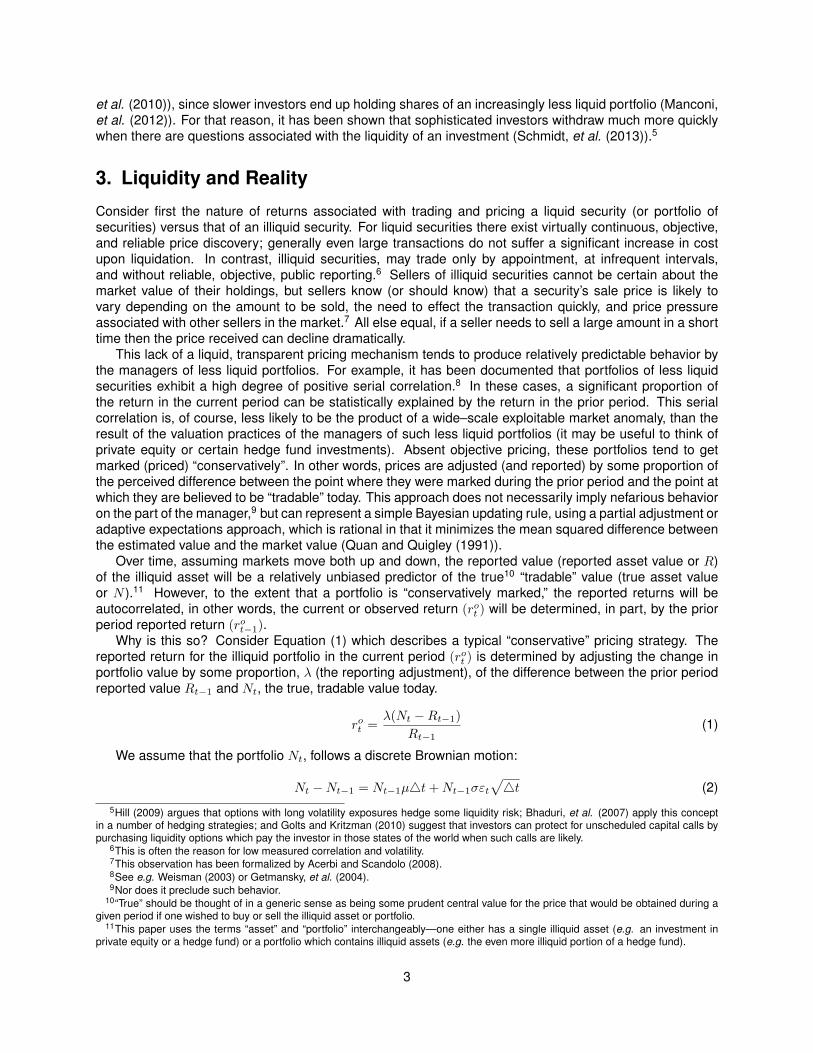
To focus on funds for which the liquidity option represented a real reduction in return, we selected hedgefunds with positive average returns and an option value greater than 1.00 (that is, where the option reducesthe expected return by 1.00% or more). This resulted in a final sample of 1,031 funds. For this sample, themean annualized return for this sample of funds was 18.75%, the mean annualized standard deviation was25.67%, and the mean serial correlation was 0.1959. The mean option value for these 1,031 hedge fundswas 15.82, implying an actual liquidity–adjusted mean return of 2.93% on an annualized basis—a sharpcontrast from the supposed 18.75%.29 Narrowing the sample allows us to further explore the applicationof the liquidity option to real data. For example Figure (6) confirms the observation made earlier with theHFRI indices—serial correlation alone is not a proxy for the value of the liquidity option. And, as shown inFigure (7) serial correlation does not have a particularly strong relationship to maximum drawdown.

Figure 6: Option Value verses Serial Correlation

0.1 0.2 0.3 0.4 0.5 0.6 0.7 0.8

10

20

30

40

50

60

70

80

Serial Correlation

Op

tio

n V

alu

e (

$)

27This is approximately the average risk free rate for the period.281,357 of the funds had a zero option value.29Of course, there is a purposeful selection bias here.

11

Figure 7: Maximum Drawdown verses Serial Correlation

0.1 0.2 0.3 0.4 0.5 0.6 0.7 0.8

10

20

30

40

50

60

70

80

90

Maxim

um

Dra

wd

ow

n (

%)

Serial Correlation

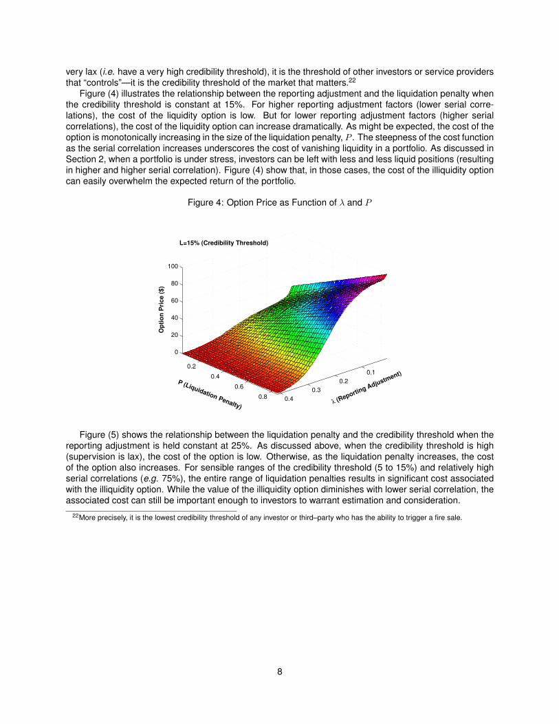
From Figure (8) we can tell that the mean return of the fund has only a weak relationship with the value ofthe liquidity option, and from Figure (9), that the mean return has no relationship with maximum drawdown.

Figure 8: Option Value verses Average Return

1 2 3 4 5 6 7

10

20

30

40

50

60

70

80

Op

tio

n V

alu

e (

$)

Average Monthly Return (%)

12

Figure 9: Maximum Drawdown verses Average Return

1 2 3 4 5 6 7

10

20

30

40

50

60

70

80

90

Maxim

um

Dra

wd

ow

n (

%)

Average Monthly Return (%)

As we would expect from standard option pricing theory, the value of the liquidity option has an extremelystrong relationship with the volatility, shown in Figure (10). However, Figure (11) demonstrates that there islittle relationship between the maximum drawdown experienced in the the hedge fund sample and volatility,since the vast majority of drawdowns occur with volatilities (monthly standard deviations) less that 12.5%.So while volatility of returns is an important determinant of the value of the liquidity option, it appears to beunrelated to drawdown.

Figure 10: Option Value verses Volatility

5 10 15 20 25 30 35

20

40

60

80

Volatility of Monthly Returns (%)

Op

tio

n V

alu

e (

$)

13

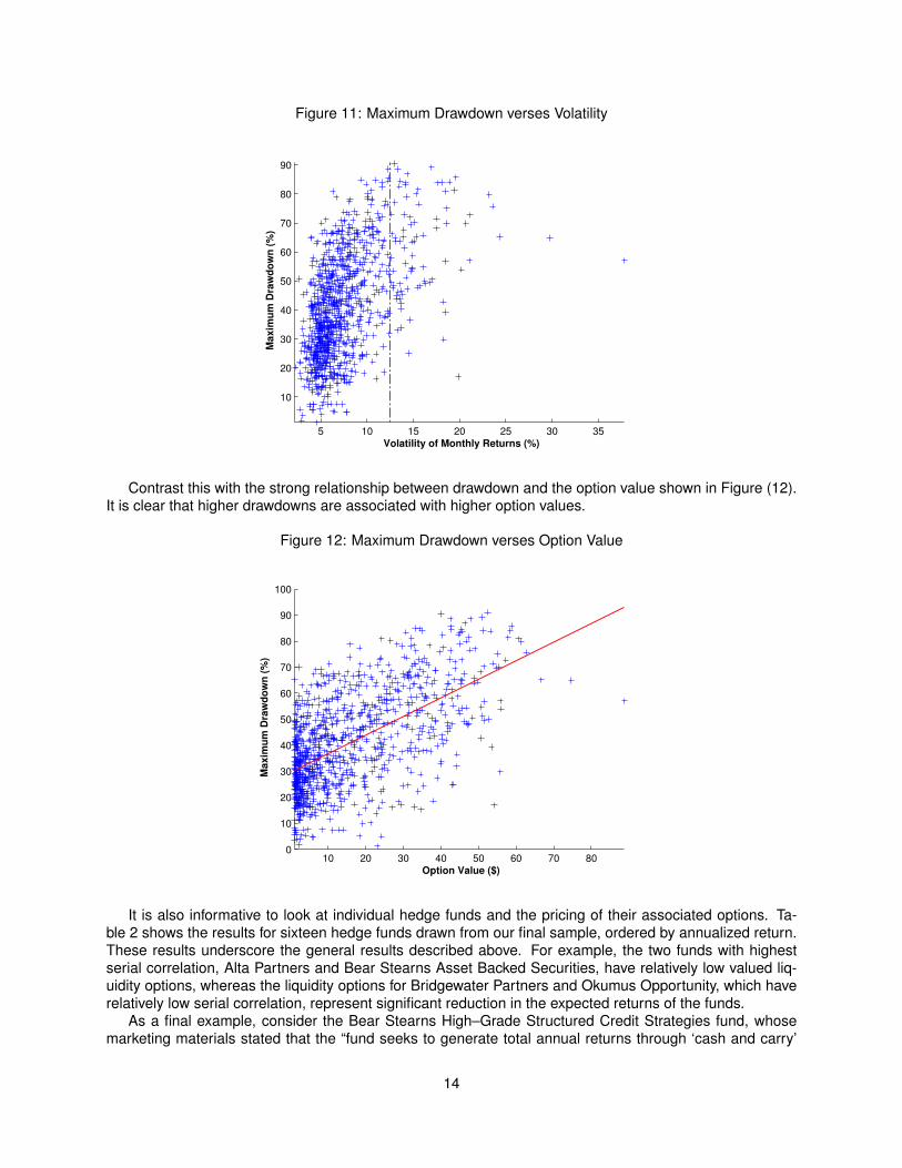
Figure 11: Maximum Drawdown verses Volatility

5 10 15 20 25 30 35

10

20

30

40

50

60

70

80

90

Maxim

um

Dra

wd

ow

n (

%)

Volatility of Monthly Returns (%)

Contrast this with the strong relationship between drawdown and the option value shown in Figure (12).It is clear that higher drawdowns are associated with higher option values.

Figure 12: Maximum Drawdown verses Option Value

10 20 30 40 50 60 70 800

10

20

30

40

50

60

70

80

90

100

Option Value ($)

Maxim

um

Dra

wd

ow

n (

%)

It is also informative to look at individual hedge funds and the pricing of their associated options. Ta-ble 2 shows the results for sixteen hedge funds drawn from our final sample, ordered by annualized return.These results underscore the general results described above. For example, the two funds with highestserial correlation, Alta Partners and Bear Stearns Asset Backed Securities, have relatively low valued liq-uidity options, whereas the liquidity options for Bridgewater Partners and Okumus Opportunity, which haverelatively low serial correlation, represent significant reduction in the expected returns of the funds.

As a final example, consider the Bear Stearns High–Grade Structured Credit Strategies fund, whosemarketing materials stated that the “fund seeks to generate total annual returns through ‘cash and carry’

14

Table 2: Select Hedge Fund Performance and Adjusted Performance

Fund Name Annualized Return Serial Correlation Option Value Adjusted Annual ReturnDeephaven Credit Opportunities 1.88% 0.42 $1.32 0.56%Bridgewater Partners 3.58% 0.20 $8.21 -4.62%Thames River European A (EUR) 6.76% 0.03 $1.28 5.47%Thames River Property Growth & Income (EUR) 7.24% 0.43 $1.64 5.60%Glenrock Global Partners (BVI), Inc. 7.42% 0.11 $1.01 6.40%Everest Capital Intl. 8.31% 0.27 $9.34 -1.03%Rocker Partners 9.42% 0.09 $7.46 1.96%Alta Partners L.P. (Onshore) 11.13% 0.64 $1.67 9.46%Rainbow Global High Yield (USD) 16.03% 0.28 $14.31 1.71%Marathon Emerging Markets 16.20% 0.23 $20.05 -3.85%Bear Stearns Asset Backed Securities LP 24.86% 0.60 $2.24 22.61%Okumus Opportunity A 27.53% 0.04 $36.48 -8.95%Viaticus 31.22% 0.05 $33.03 -1.81%Lancer Offshore 33.63% 0.16 $9.68 23.95%Galleon Omni Technology (B) 40.25% 0.13 $45.76 -5.50%Infinity Emerging Opportunities 74.16% 0.12 $88.80 -14.64%

15

transactions and capital markets arbitrage.”30 It further stated that “the Fund generally invests in high qualityfloating rate structured finance securities.” The High–Grade Structured Credit Strategies fund is a posterchild for a fire sale and rapid liquidation. As subprime mortgage delinquencies grew, the value of CDOsheld by the fund dropped. The fund’s prime brokers asked for more cash collateral. The fund attemptedto meet those collateral calls through liquidation of assets in a rapidly deteriorating market, but values fellquickly and collateral requirements rose rapidly, leading to eventual collapse. The fund failed in spite of anattempt to stabilize the fund value through the substantial injection of capital by Bear Stearns.

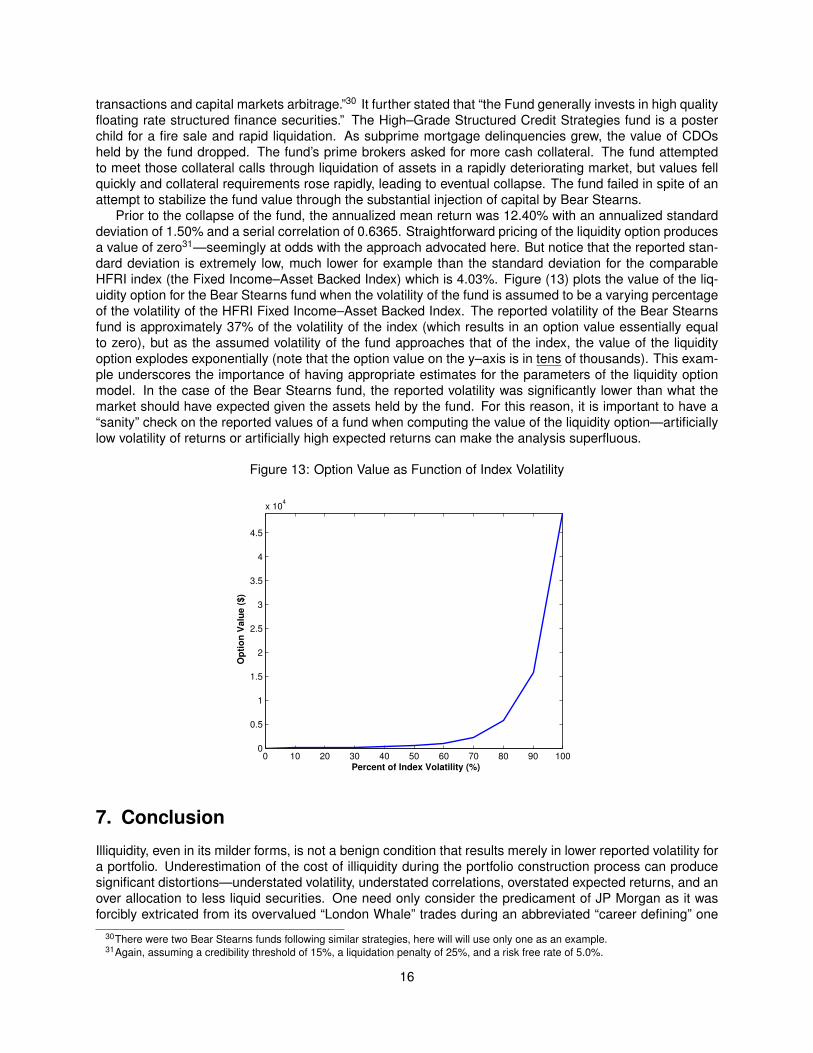
Prior to the collapse of the fund, the annualized mean return was 12.40% with an annualized standarddeviation of 1.50% and a serial correlation of 0.6365. Straightforward pricing of the liquidity option producesa value of zero31—seemingly at odds with the approach advocated here. But notice that the reported stan-dard deviation is extremely low, much lower for example than the standard deviation for the comparableHFRI index (the Fixed Income–Asset Backed Index) which is 4.03%. Figure (13) plots the value of the liq-uidity option for the Bear Stearns fund when the volatility of the fund is assumed to be a varying percentageof the volatility of the HFRI Fixed Income–Asset Backed Index. The reported volatility of the Bear Stearnsfund is approximately 37% of the volatility of the index (which results in an option value essentially equalto zero), but as the assumed volatility of the fund approaches that of the index, the value of the liquidityoption explodes exponentially (note that the option value on the y–axis is in tens of thousands). This exam-ple underscores the importance of having appropriate estimates for the parameters of the liquidity optionmodel. In the case of the Bear Stearns fund, the reported volatility was significantly lower than what themarket should have expected given the assets held by the fund. For this reason, it is important to have a“sanity” check on the reported values of a fund when computing the value of the liquidity option—artificiallylow volatility of returns or artificially high expected returns can make the analysis superfluous.

Figure 13: Option Value as Function of Index Volatility

0 10 20 30 40 50 60 70 80 90 1000

0.5

1

1.5

2

2.5

3

3.5

4

4.5

x 104

Op

tio

n V

alu

e (

$)

Percent of Index Volatility (%)

7. Conclusion

Illiquidity, even in its milder forms, is not a benign condition that results merely in lower reported volatility fora portfolio. Underestimation of the cost of illiquidity during the portfolio construction process can producesignificant distortions—understated volatility, understated correlations, overstated expected returns, and anover allocation to less liquid securities. One need only consider the predicament of JP Morgan as it wasforcibly extricated from its overvalued “London Whale” trades during an abbreviated “career defining” one

30There were two Bear Stearns funds following similar strategies, here will will use only one as an example.31Again, assuming a credibility threshold of 15%, a liquidation penalty of 25%, and a risk free rate of 5.0%.

16

month period, or for the investors in “quant” hedge funds in August of 2008 to appreciate how large thesecosts can be. To adjust properly for the embedded risks of illiquidity, we propose a straightforward barrieroption pricing model which provides an objective framework for incorporating market data and investorexperience; and thereby allows institutions to evaluate the true cost of illiquidity in their investments.

It is also important for investors to recognize that the liquidity of an investment is not necessarily constantthrough time. When a portfolio comes under funding stress, the easiest and quickest way to alleviatethat stress is to sell the most liquid assets in the portfolio. But as liquid assets are sold, the portfoliobecomes even more illiquid, generally over short time horizons—driving up, sometimes rapidly, the cost ofthe embedded illiquidity option.

As this paper has shown illiquidity in the market place has discernible costs. The barrier option pricingmethodology described here can provide both a screen and a rigorous adjustment mechanism for evaluatinginvestments which appear attractive, but may actually be unduly risky. Thus in the case of the Bear Stearnsfund discussed above, a modest upward adjustment to the fund’s reported volatility revealed an embeddedoption cost that dwarfed the reported returns, because of the fund’s highly serially correlated returns. Thispaper’s rigorous framework for assessing liquidity provides the fund manager with the means to make anannualized adjustment to reported returns that corrects for illiquidity.

17

Appendix I: Matlab Code

% Illiquidity_Option.m

% From the paper "Forced Liquidations, Fire Sales, and the Cost of Illiquidity",

% by Richard R. Lindsey and Andrew W. Weisman

% Set basic parameters

S0 = 100; % Starting value of portfolio

mu = 0.05; % Expected return of the portfolio

sigma = 0.25; % Adjusted volatility of the portfolio using Geltner (1993) methodology

irate = 0.02; % Riskless interest rate

lambda = 0.25; % Reporting adjustment (1- first order serial correlation)

threshold = 0.10; % Estimate of market credibility threshold

penalty = 0.25; % Estimate of liquidation penalty

T = 1; % One year

NSteps = 52; % Number of pricing periods (52 weeks)

NRepl = 1000000; % Number of replications in the Monte-Carlo simulation

dt = T/NSteps;

index = NSteps+1;

% Pre-allocate and initialize

SPaths = zeros(NRepl, index); % SPaths are the actual values

SPaths(:,1) = S0;

LPaths = zeros(NRepl, index); % LPaths are the conservative values

LPaths(:,1) = S0;

% Monte-Carlo Simulation

nudt = (mu-0.5*sigma^2)*dt;

sidt = sigma*sqrt(dt);

for i = 1:NRepl

for j = 1:NSteps

SPaths(i,j+1) = SPaths(i,j)*exp(nudt + sidt*randn);

LPaths(i,j+1) = LPaths(i,j)+lambda*(SPaths(i,j)-LPaths(i,j));

end

end

% Over or understatement compared to credibility threshold

diff = ((LPaths-SPaths)./SPaths)*100;

[row,col] = find(diff >= threshold*100);

urows = unique(row);

firsttime = zeros(length(urows),1);

for i = 1:length(urows)

firsttime(i) = find(diff(urows(i),:)>=threshold*100,1);

end

% Preallocate

LiqLoss = zeros(length(urows),1);

OverState = zeros(length(urows),1);

OptionVal = zeros(length(urows),1);

% Determining the cost of the illiquidity option

for i = 1:length(urows)

LiqLoss(i) = SPaths(urows(i),firsttime(i))*penalty;

18

OverState(i) = diff(urows(i),firsttime(i));

OptionVal(i) = (LiqLoss(i) + OverState(i)) * exp(-irate*(firsttime(i)/NSteps));

end

CostOption = sum(OptionVal)/NRepl;

19

Appendix II:

The true value of the fund at time t is given by:

Nt = Nt−1(1 + rt)

rearranging to get the true return rt:

rt =NtNt−1

− 1

The reported value of the fund is:

Rt = λ(Nt−1(1 + rt)−Rt−1) +Rt−1

which can be rearranged to provide the observed return rot

rot =RtRt−1

− 1

=λ(Nt−1(1 + rt)−Rt−1)

Rt−1

= λ

(Nt−1

Rt−1

)(1 + rt)− λ

Note that the observed first–order serial correlation is given by:

ρo1,t =Cov(rot , r

ot−1)

Var(rot )=

E[(rot − E [rot ])

(rot−1 − E

[rot−1

])]E[(rot − E [rot ])

2] (5)

We note that the expectations of the observed return series at times t and t− 1 are given by:

E[rot ] = λ

(Nt−1

Rt−1

)(1 +m)− λ

E[rot−1] = λ

(Nt−2

Rt−2

)(1 +m)− λ

Where m is given by:

m = µ− σ2

2

Working with the denominator of Equation (5):

E[(rot − E [rot ])

2]

E

[([λ

(Nt−1

Rt−1

)(1 + rt)− λ

]−[λ

(Nt−1

Rt−1

)(1 +m)− λ

])2]

λ2(Nt−1

Rt−1

)2

E[((1 + rt)− (1 +m))

2]

λ2(Nt−1

Rt−1

)2

E[(1 + rt)

2 − 2(1 + rt)(1 +m) + (1 +m)2]

20

λ2(Nt−1

Rt−1

)2 (E[(1 + rt)

2]− 2(1 +m)(1 +m) + (1 +m)2

)λ2(Nt−1

Rt−1

)2 (E[1 + 2rt + r2t

]− (1 +m)2

)λ2(Nt−1

Rt−1

)2 (1 + 2m+ σ2 +m2 − (1 +m)2

)λ2(Nt−1

Rt−1

)2 ((1 +m)2 + σ2 − (1 +m)2

)λ2(Nt−1

Rt−1

)2

σ2

And now the numerator of Equation (5):

E

[(rot − E [rot ])

(rot−1 − E

[rot−1

])]

E

[rot r

ot−1 − E [rot ] r

ot−1 − E

[rot−1

]rot + E [rot ] E

[rot−1

]]E[rot r

ot−1

]− E [rot ] E

[rot−1

]− E [rot ] E

[rot−1

]+ E [rot ] E

[rot−1

]E[rot r

ot−1

]− E [rot ] E

[rot−1

]E

[(λ

(Nt−1

Rt−1

)(1 + rt)− λ

)(λ

(Nt−2

Rt−2

)(1 + rt−1)− λ

)]− E [rot ] E

[rot−1

]E

[λ

(Nt−1

Rt−1

)λ

(Nt−2

Rt−2

)(1 + rt)(1 + rt−1)

]− λE [rot ]− λ2 − λE

[rot−1

]− λ2 + λ2 − E [rot ] E

[rot−1

]E

[λ

(Nt−1

Rt−1

)λ

(Nt−2

Rt−2

)(1 + rt)(1 + rt−1)

]

−

(λE [rot ] + λE

[rot−1

]+ λ2 + E [rot ] E

[rot−1

])

E

[λ

(Nt−1

Rt−1

)λ

(Nt−2

Rt−2

)(1 + rt)(1 + rt−1)

]

−

((E [rot ] + λ)

(E[rot−1

]+ λ))

E

[λ

(Nt−1

Rt−1

)λ

(Nt−2

Rt−2

)(1 + rt)(1 + rt−1)

]

−

((λ

(Nt−1

Rt−1

)(1 +m)− λ+ λ

)(λ

(Nt−2

Rt−2

)(1 +m)− λ+ λ

))

E

[λ

(Nt−1

Rt−1

)λ

(Nt−2

Rt−2

)(1 + rt)(1 + rt−1)

]

−

(λ

(Nt−1

Rt−1

)λ

(Nt−2

Rt−2

)(1 +m)2

)

λ

(Nt−1

Rt−1

)λ

(Nt−2

Rt−2

)E [1 + rt + rt−1 + rtrt−1]

21

−

(λ

(Nt−1

Rt−1

)λ

(Nt−2

Rt−2

)(1 +m)2

)

λ

(Nt−1

Rt−1

)λ

(Nt−2

Rt−2

)(1 +m+m+ E [rtrt−1]

)

−

(λ

(Nt−1

Rt−1

)λ

(Nt−2

Rt−2

)(1 +m)2

)

λ

(Nt−1

Rt−1

)λ

(Nt−2

Rt−2

)(1 + 2m+m2 −m2 + E [rtrt−1]

)

−

(λ

(Nt−1

Rt−1

)λ

(Nt−2

Rt−2

)(1 +m)2

)

λ

(Nt−1

Rt−1

)λ

(Nt−2

Rt−2

)((1 +m)2 + E [rtrt−1]−m2

)

−

(λ

(Nt−1

Rt−1

)λ

(Nt−2

Rt−2

)(1 +m)2

)

λ

(Nt−1

Rt−1

)λ

(Nt−2

Rt−2

)(E [rtrt−1]−m2

)We can now write the observed first–order auto correlation as

ρo1,t =

λ(Nt−1

Rt−1

)λ(Nt−2

Rt−2

)(E [rtrt−1]−m2

)λ2(Nt−1

Rt−1

)2σ2

=

(Nt−2

Rt−2

)(E [rtrt−1]−m2

)(Nt−1

Rt−1

)σ2

=

(Nt−2

Rt−2

)(Nt−1

Rt−1

)(E [rtrt−1]−m2

σ2

)

=

(Nt−2

Rt−2

)(Nt−1

Rt−1

)ρ1,t=

(Nt−2

Nt−1

)(Rt−1

Rt−2

)ρ1,t

=

(1 + rot−1

1 + rt−1

)ρ1,t

=

(ρ1,t

1 + rt−1

)[1 + λ

(Nt−2

Rt−2

)(1 + rt−1)− λ

]=

(ρ1,t

1 + rt−1

)(1− λ) + λ

(Nt−2

Rt−2

)ρ1,t

where ρ1,t is the actual first–order serial correlation in the underlying series rt. Note that:

Nt = N0

t∏τ=1

(1 + rτ )

22

and

Rt = λ(Nt−1(1 + rt)−Rt−1) +Rt−1

= λNt +Rt−1(1− λ)= λ(1− λ)0Nt + λ(1− λ)Nt−1 + λ(1− λ)2Nt−2 + (1− λ)3Rt−3

= λ

[t∑

n=0

(1− λ)nNt−n

]

= λ

[t∑

n=0

(1− λ)nN0

t−n∏τ=1

(1 + rτ )

]

Going back to our expression for ρo1,t,

ρo1,t =

(ρ1,t

1 + rt−1

)(1− λ) + λ

(Nt−2

Rt−2

)ρ1,t

=

(ρ1,t

1 + rt−1

)(1− λ) +

(N0

∏t−2τ=1(1 + rτ )∑t−2

n=0(1− λ)nN0

∏t−n−2τ=1 (1 + rτ )

)ρ1,t

=

(ρ1,t

1 + rt−1

)(1− λ) +

( ∏t−2τ=1(1 + rτ )∑t−2

n=0(1− λ)n∏t−n−2τ=1 (1 + rτ )

)ρ1,t

= a(1− λ) + b

Note that both a and b are less than 1.0.

23

Bibliography

Anson. M., “Measuring a Premium for Liquidity Risk,” The Journal of Private Equity, Spring 2010, pp.6–16.

Anson, M., “Risk Management and Risk Budgeting in Real Estate and Other Illiquid Asset Classes,”CFA Institute, March 2013, pp. 1–11.

Acerbi, C., and Scandolo, G., “Liquidity Risk Theory and Coherent Measures of Risk,” QuantitativeFinance, 8(7), October 2008, pp. 681–692.

Amihud, Y., H. Mendelson, and Pedersen L., “Liquidity and Asset Prices,” Foundations andTrends in Finance, 1(4), 2005, pp. 269–364.

Ang, A., Papanikolaou, D., and Westerfield, M., “Portfolio Choice with Illiquid Assets,” Working Paper,2011, SSRN-id1697784.

Ang, A., and Bollen, N., “Locked Up by a Lockup: Valuing Liquidity as a Real Option,” FinancialManagement, 39, 2010, pp. 1069–1095.

Bhaduri, R., Meissner, G., and Youn, J., “Hedging Liquidity Risk,” Journal of Alternative Investments,10(3), Winter 2007, pp. 80–90.

Bhattacharya, U., Lee, J.H., and Pool, V., “Conflicting Family Values in Mutual Fund Families,” Journalof Finance, 68(1), 2013, pp. 173–200.

Bollen, N., and Pool, V., “Conditional Return Smoothing in the Hedge Fund Industry,” Journal of Fi-nancial and Quantitative Analysis, 43, June 2008, p. 267–298.

Boyson, N., Stahel, C., and Stulz, R., “Hedge Fund Contagion and Liquidity Shocks,” Journal ofFinance, 65(5), 2010, pp. 1789–1816.

Brunnermeier, M., and Pedersen, L., “Market Liquidity and Funding Liquidity,” Review of FinancialStudies, 22(6), 2009, pp. 2201–2238.

Chen, Q., Goldstein, I., and Jiang, W., “Payoff Complementarities and Financial Fragility: Evidencefrom Mutual Fund Outflows,” Journal of Financial Economics, 97, 2010, pp. 239–262.

Derman, E., “A Simple Model for the Expected Premium for Hedge Fund Lockups,” Journal of Invest-ment Management, 5, 2007, pp. 5–15.

Derman, E., Park, K. S., and Whitt, W., “Markov Chain Models to Estimate the Premium for ExtendedHedge Fund Lockups,” Wilmott Journal, 1(5–6), 2009, pp. 263–293.

Garleanu, N., and Pedersen, L., “Margin-Based Asset Pricing and Deviations from the Law of OnePrice,” Working Paper, 2009, NYU–Stern.

Geltner, D., “Smoothing in Appraisal–Based Returns,” Journal of Real Estate Finance and Economics,4, 1991, pp. 327–345.

Geltner, D., “Estimating Market Values from Appraisal Values without Assuming an Efficient Market,”Journal of Real Estate Research, 8, 1993, pp. 325-345.

Gennaioli, N., Shleifer, A., and Vishny R., “Neglected Risks, Financial Innovation, and FinancialFragility,” Journal of Financial Economics, 104(3), 2012, pp. 452–468.

Getmansky, M., Lo, A., and Makarov, I., “An Econometric Model of Serial Correlation and Illiquidity inHedge Fund Returns,” Journal of Financial Economics, 74(3), December 2004, pp. 529–609.

Golts, M. and Kritzman, M., “Liquidity Options,” The Journal of Derivatives, Fall 2010, pp. 80–89.

24

Hamonno, G., and Thanh, N.T., “The Necessity to Correct Hedge Fund Returns: Empirical Evidenceand Correction Method,” Working Paper, 2007, LaRochelle Business School.

Hill, J.M., “A Perspective on Liquidity Risk and Horizon Uncertainty,” The Journal of Portfolio Manage-ment, Summer 2009, 35(4), pp. 60–68.

JP Morgan Asset Management, “Long Term Capital Market Return Assumptions,” 2012 edition.

Keane, F., “Securities Loans Collateralized by Cash: Reinvestment Risk, Run Risk, and IncentiveIssues,” Federal Reserve Bank of New York, Current Issues in Economics and Finance 19(3), 2013.

Kinlaw, W., Kritzman, M., and Turkington, D., “Liquidity and Portfolio Choice: A Unified Approach”,The Journal of Portfolio Management, 39(2), 2013, pp. 19–27.

Leibowitz, L., and Bova, A., “Portfolio Liquidity,” 2009, Morgan Stanley Research.

Leising, M., and Hurtado, P., “JP Morgan May Distance Trades from Bank with Intent Claim,”Bloomberg News, July 15, 2012.

Lewis, M., Boomerang: Travels in the New Third World, W. W. Norton & Company, Inc. 2011.

Lo, A., Petrov, C., and Wierzbicki, M., “It’s 11pm—Do You Know Where Your Liquidity Is? The Mean–Variance Liquidity Frontier”, Journal of Investment Management, 1, 2003, pp. 55–93.

Longstaff, F. A., “How Much Can Marketability Affect Security Values?,” Journal of Finance, 50, 1995,pp. 1767–1774.

Manconi, A., Massa, M., and Yasuda, A., “The Role of Institutional Investors in Propagating the Crisisof 2007–2008,” Journal of Financial Economics, 104(3), 2012, pp. 491–518.

Mitchell, M., Pedersen, L., and Pulvino, T., “Slow Moving Capital,” American Economic Review, 97(2),2007, pp. 215–220.

Office of Financial Research, “Asset Management and Financial Stability,” US Department of Treasury,September 2013.

Okunev, J., and White, D., “Hedge Fund Risk Factors and Value at Risk of Credit Trading Strategies,”Working Paper, 2003, University of New South Wales.

Quan, D., and Quigley, J., “Price Formation and the Appraisal Function in Real Estate Markets,” Jour-nal of Real Estate Finance and Economics, 4(2), 1991, pp. 127–146.

Ramadorai, T., “The Secondary Market for Hedge Funds and the Closed–Hedge Fund Premium,”Working Paper, 2008, University of Oxford.

Schmidt, L., Timmermann, A., and Wermers, R., “Runs on Money Market Mutual Funds,” WorkingPaper, 2013, SSRN-id2024282.

Scholes, M., and Williams, J., “Estimating Betas From Nonsynchronous Data,” Journal of FinancialEconomics, 5(3), December 1977, pp. 309–327.

Scholes, M., “The Near Crash of 1998: Crisis and Risk Management,” American Economic Associa-tion Papers and Proceedings, 90, 2000, pp. 17–21.

Siegel, J., “Alternatives and Liquidity: Will Spending and Capital Calls Eat Your Modern Portfolio,”Journal of Portfolio Management, Fall, 2008, pp. 103–114.

Sparrow, C. and Ilijanic, D., “The Value of Liquidity”, The Journal of Trading, Winter 2010, pp. 10–15.

Weisman, A., “Informationless Investing and Hedge Fund Performance Measurement Bias,” Journalof Portfolio Management, Summer 2002, pp. 80–91.

25