USGS Science Strategy to Support U.S. Fish and Wildlife Service Polar Bear Listing Decision

Forecasting the Range-wide Status of Polar Bears at Selected Times in the 21st Century

By Steven C. Amstrup1, Bruce G. Marcot2, and David C. Douglas3

Administrative Report

U.S. Department of the Interior U.S. Geological Survey

U.S. Department of the Interior DIRK KEMPTHORNE, Secretary

U.S. Geological Survey Mark D. Myers, Director

U.S. Geological Survey, Reston, Virginia: 2007

U.S. Geological Survey Administrative Reports are considered to be unpublished and may not be cited or quoted except in follow-up administrative reports to the same federal agency or unless the agency releases the report to the public.

Any use of trade, product, or firm names is for descriptive purposes only and does not imply endorsement by the U.S. Government.

Author affiliations:

1 U.S. Geological Survey, Alaska Science Center, Anchorage 2 USDA Forest Service, Pacific Northwest Research Station, Portland, Oregon 3 U.S. Geological Survey, Alaska Science Center, Juneau

ii

Contents

Abstract................................................................................................................................................................................ 1 Introduction ......................................................................................................................................................................... 2

Study Objective ............................................................................................................................................................... 2 Background biology ....................................................................................................................................................... 2

Methods ............................................................................................................................................................................... 5 Polar Bear Ecoregions ................................................................................................................................................... 6 Modeling........................................................................................................................................................................... 8

Overview....................................................................................................................................................................... 8 Sea-ice habitat variables .......................................................................................................................................... 8 Carrying Capacity Model ......................................................................................................................................... 10

Habitat amount ...................................................................................................................................................... 10 Change in habitat amount .................................................................................................................................... 10 Polar bear densities .............................................................................................................................................. 11 Polar bear carrying capacity .............................................................................................................................. 11 Percent change in carrying capacity ................................................................................................................ 12 Assigning Status Categories Based on Carrying Capacity Change ............................................................12

Bayesian Network Population Stressor Model ................................................................................................... 12 What are Bayesian network models? ............................................................................................................... 13 Use of Bayesian networks in ecological modeling......................................................................................... 13 Structuring the Bayesian network population stressor model for polar bears .........................................14 Parameterizing the Bayesian network model .................................................................................................. 15 Bayesian network model output states ............................................................................................................ 16

Node C4: Numerical Response ....................................................................................................................... 16 Node C3: Distribution Response ..................................................................................................................... 17 Node D1: Overall Population Outcome .......................................................................................................... 17

Results ................................................................................................................................................................................ 19 Forecasted 21st Century Polar Bear Carrying Capacity .......................................................................................... 19

Habitat area and change ......................................................................................................................................... 19 Polar bear carrying capacity .................................................................................................................................. 20

Bayesian Network Model Forecast of the 21st Century Status of Polar Bears ..................................................20 Sensitivity Structure of the Bayesian Network Population Stressor Model ..................................................21

Discussion .......................................................................................................................................................................... 22 Types and Implications of Uncertainty ..................................................................................................................... 22 Forecasted 21st Century Polar Bear Carrying Capacity .......................................................................................... 24 Bayesian Network Model Forecast of the 21st Century Status of Polar Bears ..................................................27

Next steps in the BN model development ............................................................................................................ 27 BN model projected outcomes ............................................................................................................................... 28 Sensitivity analyses .................................................................................................................................................. 29

Strength of evidence of BN model projections ....................................................................................................... 31 Conclusion ......................................................................................................................................................................... 35 Acknowledgements ......................................................................................................................................................... 36

iii

References Cited .............................................................................................................................................................. 36 Appendix 1. Results of sensitivity analyses of the Bayesian network population stressor model .................... 97 Appendix 2. Documentation of the Bayesian network polar bear population stressor model. ....................... 100 Appendix 3. Probability tables for each node in the Bayesian network model .................................................. 109 Figures

Figure 1. Map of four polar bear ecoregions to which we refer in this report. Ecoregions were established by grouping recognized subpopulations which share seasonal patterns of ice motion and distribution. ...... 82 Figure 2. Linkages followed in this report, from available information on sea ice polar bears and other environmental correlates, and leading to projections of future polar bear carrying capacity and overall population outcome. ........................................................................................................................................................ 83 Figure 3. (a) Average summer and winter sea ice extent in the entire polar basin (divergent and convergent regions) expressed in square km (left) and as a percent change relative to each model’s 1990-1999 mean for 20th century hindcasts (right). (b) Average RSF habitat values for summer and winter expressed in raw RSF units (left) and percent change to each model’s 1990-1999 mean for the 20th century hindcasts (right). 84 Figure 4. The basic influence diagram for the Bayesian network polar bear population stressor model showing the role of 4 listing factor categories used by U.S. Fish and Wildlife Service. ..................................... 85 Figure 5. The full Bayesian network population stressor model developed to evaluate overall population outcome. ............................................................................................................................................................................. 86 Figure 6. Annual (12-month sum) polar bear habitat area Ht,G at t years -10 and 0 from satellite data and 0, 45, 75, and 100 from minimum, ensemble mean, and maximum global change model (GCM) runs, in four geographic regions G and all regions combined (see Table 4). .............................................................................. 87 Figure 7. Percent change in polar bear habitat amounts CHt,G at t years -10 and 0 from satellite data and 0, 45, 75, and 100 from minimum, ensemble mean, and maximum global change model (GCM) runs, in four geographic regions G and all regions combined, normalized to 0% change at year 0 (see Table 4). .............. 88

normFigure 8. Normalized polar bear carrying capacity Kt ,G at t years -10 and 0 based on habitat amount from

satellite data at year -10, empirical bear counts at year 0, and habitat amounts at years 0, 45, 75, and 100 from minimum, ensemble mean, and maximum global change model (GCM) runs, in four geographic regions G and all regions combined (see Table 6). ................................................................................................................... 89 Figure 9. Polar bear carrying capacity trends CKt,G at t years -10 and 0 based on carrying capacity values from Figure 8, in four geographic regions G and all regions combined, normalized to 0% change at year 0 (see Table 6). ..................................................................................................................................................................... 90 Figure 10. Projected polar bear population outcomes of Bayesian network model for 4 ecoregions at 5 time periods relative to present. ............................................................................................................................................. 91 Figure 11. Projected probabilities of the “extinct” overall population outcome (node D1 in Fig. 5), from the Bayesian network population stressor model. ........................................................................................................... 92 Figure 12. Cumulative sensitivity of overall population outcome (node D1, Fig. 5) to all input variables (yellow boxes, Fig. 5), in the Bayesian network population stressor model. ......................................................... 93 Figure 13. Mean (SE) area of optimal RSF polar bear habitat in the polar basin by season and decadal time period (top), and percentage change in the same values (bottom), from ensemble mean of 10 IPCC AR-4 general circulation models. ............................................................................................................................................ 94 Figure 14. Probability of “extinct” outcomes projected by a Bayesian network (BN) polar bear population stressor model. Projections include 4 ecoregions, and 3 future time periods relative to present. ................... 95

iv

Figure 15. Area of sea ice extent (>50% ice concentration) on August 23, 2007, compared to 10 IPCC AR-4 GCM mid-century projections of ice extent for September 2045–2054 (mean ± 1 sd, n = 10 years). ................96

Tables

Table 1. Ten IPCC AR-4 GCMs whose sea ice simulations and projections were used to define ice covariates for polar bear RSF models: IPCC model ID, country of origin, approximate grid resolution (degrees), forcing scenario, and the number of runs used for the polar bear studies........................................47 Table 2. Composite summary categories of polar bear carrying capacity change from present levels, based

Table 4. Amount, percent change, and summary of change in polar bear habitat forecasted by the

Table 6. Polar bear carrying capacity forecast for each ecoregion, time period, and modeling

Table 7. Overall summary of change in total polar bear carrying capacity from present levels (based on

Table 8. Results of the Bayesian network population stressor model, showing the most probable outcome state, and probabilities of each state (larger, same as now, smaller, rare, and extinct), for overall population

Table 9. Results of the Bayesian network population stressor model, showing the most probable outcome states, and probabilities of each state, for the distribution response and numerical response outcomes

Table 10. Results of the Bayesian network population stressor model, showing the most probable outcome states, and probabilities of each state, for habitat threats and director mortalities summary variables

Table 11. Results of the Bayesian network population stressor model, showing the most probable outcome

Table 12. Results of the Bayesian network population stressor model, showing the most probable outcome states, and probabilities of each state, for disease/predation and other disturbance factors variables

Table 13. Results of the Bayesian network population stressor model, showing the most probable outcome

on categories of composite habitat change and composite carrying capacity change. ...................................48 Table 3. Input data used in the Bayesian network population stressor model (Figure 5). ..................................49

deterministic polar bear carrying capacity model. .................................................................................................... 57 Table 5. Numbers and densities of polar bears by ecoregion, based on habitat amount at year 0 (Table 4). 60

basis, by the deterministic polar bear carrying capacity model. .................................................................61

applying results of carrying capacity calculations in Table 6 to the rule set in Table 2). ...................................64

outcome (node D1; see Figure 5). .................................................................................................................................. 66

(nodes C3, C4; see Figure 5). ........................................................................................................................................... 68

(nodes F2 and A1; see Fig. 5). ......................................................................................................................................... 70

states, and probabilities of each state, for changes in foraging habitat distribution (node D; see Figure 5). . 72

(nodes A4, A6; see Figure 5). .......................................................................................................................................... 74

states, and probabilities of each state, for reproduction and vital rates (nodes U, L2; see Figure 5). ..............76 Table 14. Projected outcomes from Bayesian network population stressor model showing probabilities of overall outcome states resulting when all human factors were fixed at ‘same as now’ or ‘fewer than now.’ ........................................................................................................................................... 78 Table 15. Projected outcomes from Bayesian network population stressor model showing probabilities of overall outcome states resulting when all human factors were fixed at uniform. ..80 Appendix 1. Results of sensitivity analyses of the Bayesian network population stressor model ...................97 Appendix 2. Documentation of the Bayesian network polar bear population stressor model ........................100 Appendix 3. Probability tables for each node in the Bayesian network model ..................................................109

v

Abbreviations, Acronyms, and Symbols

Abbreviations, Acronyms, and Meaning Symbols

AR-4 IPCC Fourth Assessment Report

BB Baffin Bay IUCN polar bear subpopulation unit

BN Bayesian Network

BS Barents Sea IUCN polar bear subpopulation unit

CS Chukchi Sea IUCN polar bear subpopulation unit

DS Davis Strait IUCN polar bear subpopulation unit

EG East Greenland IUCN polar bear subpopulation unit

FB Foxe Basin IUCN polar bear subpopulation unit

GB Gulf of Boothia IUCN polar bear subpopulation unit

GCM General Circulation Model

HAD1SST Hadley Center sea ice and temperature data set

IBCAO International Bathymetric Chart of the Arctic Ocean

IPCC International Panel on Climate Change

IUCN International Union for the Conservation of Nature

KB Kane Basin IUCN polar bear subpopulation unit

KS Kara Sea IUCN polar bear subpopulation unit

LS Lancaster Sound IUCN polar bear subpopulation unit

LVS Laptev Sea IUCN polar bear subpopulation unit

MC M’Clintock Channel IUCN polar bear subpopulation unit

NASA National Space and Aeronautics Administration

NBS Northern Beaufort IUCN polar bear subpopulation unit

NW Norwegian Bay IUCN polar bear subpopulation unit

PBSG Polar Bear Specialists Group

PMW Passive Microwave

QE Queen Elizabeth Islands IUCN polar bear subpopulation unit

RSF Resource Selection Function

SBS Southern Beaufort Sea IUCN polar bear subpopulation unit

SHB Southern Hudson Bay IUCN polar bear subpopulation unit

SRES Special Report on Emissions Scenarios

SRES A1B SRES, greenhouse gas forcing scenario that assumes “business as usual”

USFWS U.S. Fish & Wildlife Service

VM Viscount Melville Sound IUCN polar bear subpopulation unit

vi

WHB Western Hudson Bay IUCN polar bear subpopulation unit

vii

Forecasting the Range-wide Status of Polar Bears at Selected Times in the 21st Century By Steven C. Amstrup, Bruce G. Marcot, and David C. Douglas

Abstract

To inform the U.S. Fish and Wildlife Service decision, whether or not to list polar bears as threatened under the Endangered Species Act (ESA), we forecast the status of the world’s polar bear (Ursus maritimus) populations 45, 75 and 100 years into the future. We applied the best available information about predicted changes in sea ice in the 21st century to current knowledge of polar bear populations and their ecological relationships to the sea ice to understand how the range-wide population of polar bears might change. We combined the world’s 19 polar bear subpopulations into 4 ecological regions based on current and projected sea ice conditions. These “ecoregions” are the (1) Seasonal Ice Ecoregion which includes Hudson Bay, and occurs mainly at the southern extreme of the polar bear range, (2) the Archipelago Ecoregion of the Canadian Arctic, (3) the Polar Basin Divergent Ecoregion where ice is formed and then advected away from near-shore areas, and (4) the Polar Basin Convergent Ecoregion where sea ice formed elsewhere tends to collect against the shore. We incorporated projections of future sea ice in each ecoregion, based on 10 general circulation models (GCMs), into two models of polar bear habitat and potential population response. First, we used a deterministic model of past, current, and future polar bear carrying capacity which assumed a linear relationship between bear density and annual average sea ice extent. Because this approach did not include seasonal changes in ice availability or other possible population stressors, it provided an optimistic view of the potential magnitude of and change in population carrying capacity by ecoregion

and time step. Second, we developed a Bayesian network (BN) model structured around population stressors that could affect the factors considered in ESA decisions. The BN model combined empirical data, interpretations of data, and professional judgment into a probabilistic framework. Although BN models can be based on the collective judgment of multiple experts, time constraints in this project allowed input from only one expert. Therefore, we consider our BN model a prototype, and we provide guidance regarding next steps necessary to further refine the model. The BN model incorporated information about annual and seasonal sea ice trends as well as potential effects of other population stressors such has harvest, disease, predation, and effects of increasing human activity in the north due to ice retreat. Under both modeling approaches, polar bear populations were forecasted to decline throughout all of their range during the 21st

century. In projections based upon ensemble mean ice predictions, the carrying capacity model forecasted potential extirpation of polar bears in the Polar Basin Divergent Ecoregion in 75 years. Projections using minimal ice levels forecasted potential extirpation in this ecoregion by year 45, whereas projections using maximal ice levels forecasted steady declines but not extirpation by year 100. Populations of polar bears in the other ecoregions were projected to decline at all time steps, with severity of decline dependent upon whether minimum, maximum or mean ice projections were used. Dominant outcomes of the BN model were for extinction of polar bear populations in the Seasonal Ice and Polar Basin Divergent Ecoregions by 45 years from present, and in the Polar Basin Convergent Ecoregion by 75 years from present. The BN model projected high non-zero

1

probabilities that Archipelago polar bears could occur at smaller numbers than now through the end of the century. Declines in ice habitat were the overriding factors determining all model outcomes. Although management of human activities could forestall extinction in the Archipelago and Polar Basin Convergent ecoregions, it could not qualitatively alter the prognosis of extinction for the Polar Basin Divergent and Seasonal Ecoregions. Similarly, model results indicated that sea ice conditions would have to be substantially better than even the most conservative GCM projections to result in a qualitatively different outcome for any of the ecoregions. Our modeling suggests that realization of the sea ice future which is currently projected, would mean loss of ≈ 2/3 of the world’s current polar bear population by mid-century.

Introduction

Study Objective

Polar bears depend upon sea ice for access to their prey and for other aspects of their life history (Stirling and Øritsland 1995; Stirling and Lunn 1997; Amstrup 2003). Observed declines in sea ice availability have been associated with reduced body condition, reproduction, survival, and population size for polar bears in parts of their range (Stirling et al. 1999; Obbard et al. 2006; Stirling and Parkinson 2006; Regehr et al. 2007b). Observed (Comiso 2006) and projected (Holland et al. 2006) sea ice declines have led to the hypothesis that the future welfare of polar bears range-wide may be diminished, and to the U.S. Fish and Wildlife Service (FWS) proposal to list the polar bear as a threatened species under the Endangered Species Act (U.S. Fish and Wildlife Service 2007). The classification as a “threatened species” requires determination that it is likely the polar bear will become an endangered species within the “foreseeable future” throughout all or a significant portion of

its range. An “endangered species” is any species that is in danger of extinction throughout all or a significant portion of its range. To help inform the final listing decision, the FWS requested that the U.S. Geological Survey (USGS) conduct additional analyses of polar bears and their sea ice habitats. Between February and August 2007, USGS and collaborators developed nine reports targeting specific questions considered especially informative to the final decision. This report, one of the nine, builds upon the other eight reports and uses other current information on polar bears to forecast the status of polar bears occurring in different parts of the Arctic at three future periods in the 21st-century.

We use the best available information and knowledge, including that derived from new studies requested by the FWS, to forecast the future status of polar bears in each of 4 ecoregions (Figure 1). We present our forecast in a “compared to now” setting where projections for the decade of 2045-2055, 2070­2080, and 2090-2100 are compared to the “present” period of 1996-2006. For added perspective we also look back to the decade of 1985-1995. Hence, we examined five time periods in total. Our view of the present and past are based on sea ice conditions derived from satellite data. Our future forecasts are based largely on information derived from general circulation model (GCM) projections of the extent and spatiotemporal distribution of sea ice.

Background biology

Polar bears occur throughout portions of the Northern Hemisphere where the sea is ice-covered for all or much of the year. Polar bear genetics indicate that the species branched off from brown bears (Ursus arctos) and invaded an open niche on the surface of the sea ice during maximal extent of the continental ice sheets in the very late Pleistocene. Molecular genetic techniques suggest this could have

2

occurred as long ago as 250,000 years (Amstrup 2003).Very few polar bear fossils are known, however, and those that have been discovered are relatively recent. They appear for the first time in the fossil record only 40 to 50 thousand years ago (Thenius 1953; Kurtén 1964). During their short evolutionary history, polar bears have diverged substantially from brown bears, apparently under selective pressures stemming from their specialization for capturing seals from the surface of the ice. Stanley (1979) described the many recently-evolved traits of polar bears as an example of “quantum speciation.” The dearth of polar bear fossils reflects their specialty of living on the sea ice. Remains of dead animals on the sea ice would tend to accumulate on the sea floor rather than on land where they are more accessible to human discovery.

Since moving offshore, behavioral and physical adaptations have allowed polar bears to increasingly specialize at hunting seals from the surface of the ice (Stirling 1974; Smith 1980; Stirling and Øritsland 1995). Polar bears derive essentially all of their sustenance from marine mammal prey and have evolved a strategy designed to take advantage of the high fat content of marine mammals (Best 1984). Over half of the calories in a seal carcass are located in the layer of fat between the skin and underlying muscle (Stirling and McEwan 1975). Polar bears show their preference for fat by quickly removing the fat layer from beneath the skin after they catch a seal. The high fat intake that can be achieved by specializing on marine mammal prey has allowed polar bears to thrive in the harsh Arctic environment and to become the largest of the extant Ursids (Stirling and Derocher 1990; Amstrup 2003).

Over much of their range, polar bears are dependent on one species of seal, the ringed seal (Phoca hispida). Polar bears occasionally catch belugas (Delphinapterus leucas), narwhals (Monodon monocerus), walrus (Odobenus rosmarus), and harbor seals (P. vitulina) (Smith 1985; Calvert and Stirling 1990; Smith and

Sjare 1990; Stirling and Øritsland 1995; Derocher et al. 2002). Walruses can be seasonally important in some parts of the polar bear range (Parovshchikov 1964; Ovsyanikov 1996). Bearded seals (Erignathus barbatus) can be a large part of their diet where they are common and are probably the second most common prey of polar bears (Derocher et al. 2002). Throughout most of their range, however, polar bears are most dependent upon ringed seals (Smith and Stirling 1975; Smith 1980). The relationship between ringed seals and polar bears is so close that the abundance of ringed seals in some areas appears to regulate the density of polar bears, while polar bear predation in turn, regulates density and reproductive success of ringed seals (Hammill and Smith 1991; Stirling and Øritsland 1995). Across much of the polar bear range, their dependence on ringed seals is close enough that the abundances of ringed seals can be estimated by knowing the abundances of polar bears (Stirling and Øritsland 1995; Kingsley 1998).

Polar bears rarely can catch seals on land or in open water (Furnell and Oolooyuk 1980); rather, they consistently catch seals and other marine mammals only at the air-ice-water interface. This dependence of polar bears on hunting at the ice surface, where aquatic mammals must come to breathe, is evident in the behavior of ringed seals. Steady predation pressure from polar bears over thousands of years has led ringed seals to use subnivian (below the snow) birthing lairs and to interrupt spring and summer basking with frequent periods of scanning their surroundings for bears. This is in contrast with Weddell seals (Leptonychotes weddelli), the southern hemisphere equivalent of ringed seals, which bask and give birth in the open (Stirling 1977) and can be approached by humans without reaction.

Although there are local exceptions, it appears that polar bears gain little overall benefit from alternate foods. Even in Hudson Bay where polar bears are forced onto land for

3

extended periods with access to a variety of foods including human refuse, little terrestrial food is incorporated into polar bear tissues (Ramsay and Hobson 1991). In short, maintenance of polar bear populations is dependent upon marine prey, largely ringed seals, and they are tied to the surface of the ice for effective access to those prey.

Polar bears occur in most ice-covered regions of the northern hemisphere, including the center of the polar basin (Stefansson 1921). They are not evenly dispersed throughout this area, however. Polar bears have been observed most frequently in shallow-water areas near shore and in other areas where currents and upwellings keep the winter ice cover from becoming too solidified. These shore leads and polynyas create a zone of active unconsolidated sea ice that is small in geographic area but contributes ~50% of the total productivity in Arctic waters (Sakshaug 2004). Polar bears, are most commonly observed in or near these near shore zones where ice is constantly moving, opening up and reconsolidating, rather than pelagic areas which are of lower productivity (Stirling and Smith 1975; Pomeroy 1997; Stirling 1997), and have been shown to focus their annual activity areas over these regions (Stirling et al. 1981; Amstrup and DeMaster 1988; Stirling 1990; Stirling and Øritsland 1995; Stirling and Lunn 1997; Amstrup et al. 2000, 2004a, 2005). Not surprisingly, ice over shallow waters less than 300m deep has now been shown to be the most preferred habitat of polar bears throughout the polar basin (Durner et al. 2007).

Given their wide geographic distribution, polar bears inhabit regions with very different sea ice conditions. The southern reaches of their range includes areas where sea ice is seasonal. There, polar bears are forced onto land where they are food deprived for extended periods each year. Polar bears of Hudson Bay are the best known example of this situation, but bears in Foxe Basin, Davis Strait, and Baffin Bay also are “stuck” on land for a portion of the year

when the sea ice in their area melts entirely. Other polar bears live in some of the harshest and most northerly climes of the world where the ocean is ice-covered year-round. This includes northerly regions of the Canadian Arctic archipelago and northern Greenland (Jonkel et al. 1976). Others live in the pelagic regions of the polar basin where there are strong seasonal changes in the character of the ice. There polar bears historically have remained on the advancing and retreating ice pack throughout the year, despite the sometimes very long seasonal movements required to do so (Amstrup 1986; Amstrup and DeMaster 1988; Amstrup et al. 2000). For example, sea-ice extends as much as 400 km south of the Bering Strait that separates Asia from North America, and polar bears extend their range to the southernmost extreme of the ice (Ray 1971). Because sea ice disappears from most of the Bering and Chukchi seas in summer, however, polar bears occupying these areas must move as far as 1000 km northward to stay on the retreating ice (Garner et al. 1990, 1994). In the Chukchi Sea and elsewhere, polar bears spend their summers concentrated along the edge of the persistent pack ice. Significant northerly and southerly movements appear to be dependent upon seasonal melting and refreezing of ice near shore (Amstrup et al. 2000).

Telemetry data have shown that polar bears do not wander aimlessly on the ice, nor are they carried passively with the ocean currents as previously thought (Pedersen 1945). Rather, they occupy multi-annual activity areas from which they seldom leave. Tracking data show that polar bears use seasonally preferred or “core” regions every year, despite variation in annual activity area boundaries (Amstrup et al. 2000, 2001, 2004a, 2005). This suggests that activity areas of polar bears, when viewed over multi-year periods, could be called home ranges. All areas of the home range, however, will not be used each year. Sea-ice habitat quality varies temporally as well as geographically (Stirling and Smith 1975;

4

DeMaster et al. 1980; Ferguson et al. 1997, 1998, 2000a, 2000b; Amstrup et al. 2000). In areas where sea ice cover and character are seasonally dynamic, a large multi-year home range, of which only a portion may be used in any one season or year is an important part of the polar bear life history strategy. In other regions where ice is less dynamic, smaller and less variable activity areas are common (Messier et al. 1992; Ferguson et al. 2001).

The seasonal movement patterns of polar bears serve to emphasize the role of sea-ice in their life cycle. In the Beaufort Sea, the largest monthly activity areas and highest movement rates are during June-July and November-December. This matches the temporal patterns of ice melt and freeze in the area (Gloersen et al. 1992). Polar bears catch seals mainly by still-hunting (Stirling and Latour 1978). The dynamic summer and autumn ice must minimize predictability of seal hunting opportunity. Unpredictable ice distributions could require longer bear movements and larger bear activity areas during freeze-up and break-up. From May-August, measured net monthly movements of polar bears in the Beaufort Sea were significantly to the north for all bears, and in October they moved back to the south (Stirling 1990; Amstrup et al. 2000). October has historically been the month of freeze-up in the southern Beaufort Sea. In recent years, especially, October has been the first time in months when ice is available over the shallow water near-shore. Polar bears summering on the persistent pack ice quickly move into shallow water areas as soon as new ice forms in autumn, and they disperse easterly and westerly along near shore unconsolidated ice zones during winter. Mauritzen et al. (2001, 2002) also found movement patterns that were closely tied to seasonal ice cycles in other parts of the polar basin. Polar bears, in fact, have adapted their movement strategies to accommodate a broad range of sea ice characteristics (Messier et al. 1992; Ferguson et al. 1997, 1999).

The common denominator is that polar bears make seasonal movements to maximize their foraging time on sea ice that is suitable for hunting (Amstrup 2003). Polar bears appear to require relatively high concentrations of sea ice for effective hunting. Recent observations indicate that during most of the year, these preferred hunting habitats are sea-ice areas where the ice cover is ≥50% . (Stirling et al. 1999; Durner et al. 2004, 2006, 2007).

Methods

We took two approaches to forecast how the future range-wide population of polar bears might be different than it is now. Our first method provided estimates of the maximum potential sizes of polar bear populations based on climate modeling projections of the quantity of their habitat — but in the absence of effects of any additional stressors or knowledge about changes in habitat distribution. Our second method provided estimates of how the presence of multiple stressors, including changes in the quantity of sea ice as well as its spatiotemporal distribution, may affect polar bears.

The first approach was a deterministic calculation of polar bear habitat amount and carrying capacity in each ecoregion. We used estimated numbers of polar bears currently occupying each of the world’s subpopulations, and the amount of sea-ice habitat currently in each area, to estimate the present-day polar bear density in each of 4 defined ecoregions (Figure 1). Then we multiplied the densities by the projected future (or empirically determined historic) amount of polar bear habitat in each ecoregion at various time periods, to derive the maximum potential number of bears that habitat could support. This is an estimate of polar bear carrying capacity, given the assumptions that current populations are at or near carrying capacity, that polar bear densities (number of bears per unit area) do not change, and that quality of the future habitat is equivalent to that at present. Of course, we recognize that such

5

calculations oversimplify the eventuality. Yet, these simple calculations provide approximate numerical references of polar bear numbers that help place other discussions of future change into perspective.

Our second approach, a Bayesian network (BN) population stressor model, addressed many shortcomings of the carrying capacity model by incorporating probabilistic calculations of potential effects from multiple stressors on polar bear populations. The BN model used the same projections of habitat change as in the carrying capacity model, but it also included seasonal habitat changes as well as anticipated likelihoods of changes in several other stressors (Figure 2). The BN model accommodated scenarios of whether availability of food for polar bears would likely change and whether bears might redistribute themselves because of changes in habitat. Also considered was whether changes in hunting, oil and gas development, contaminants, parasites, disease agents and other potential anthropogenic (human-caused) stressors could become more or less influential than they are now. The BN model parameterized knowledge about the effects of observed habitat changes on polar bear distribution, demography and physical condition. This included understandings gained from other studies by the USGS relative to the listing decision, and expert judgment on the effects of a variety of other factors which might alter the future for polar bears. Construction of the BN model allowed us to integrate qualitative judgments, regarding how polar bears interact with their environment, with quantitative habitat predictions in a synthetic model to provide relative probabilities of potential future outcomes. Forecasts of the future status of polar bears were based on comparisons between current and future sea ice, and on other salient changes in the polar bear’s environment that may change as the ice diminishes. Current ice conditions were extracted from data sets derived from passive microwave satellite imagery, 1979 – 2006 (http://nsidc.org/data/nsidc-0051.html).

Future ice conditions were extracted from GCM projections (https://esg.llnl.gov:8443). In addition to sea ice extent and distribution data from satellite images and GCMs, we used resource selection functions (RSFs) to identify preferred, optimal polar bear habitat. The RSFs allowed us to evaluate whether preferred sea ice habitats may change at different rates than the overall sea ice cover.

We made forecasts of the future for polar bears in each of four ecoregions. We defined the ecoregions based on observed and GCM-projected differences in sea ice, and how polar bears respond or may respond to those changes. In the following section, we provide detailed descriptions of the four polar bear ecoregions. Next, we describe the process we used to make projections of the amount and distribution of future sea ice habitat. Finally we provide details of the modeling methods we used to project the future status of polar bears.

Polar Bear Ecoregions

Polar bears are distributed throughout regions of the Arctic and subarctic where the sea is ice covered for large portions of the year. Although movements of individual polar bears overlap extensively, telemetry studies have demonstrated spatial segregation among groups or stocks of polar bears in different regions of their circumpolar range (Schweinsburg and Lee 1982; Amstrup 1986, 2000; Garner et al. 1990, 1994; Messier et al. 1992; Amstrup and Gardner 1994; Ferguson et al. 1999; Carmack and Chapman 2003). Patterns in spatial segregation suggested by telemetry data, along with information from survey and reconnaissance, marking and tagging studies, and traditional knowledge, have resulted in recognition of 19 partially discrete polar bear groups (Aars et al. 2006). There is considerable overlap in areas occupied by members of these groups (Amstrup et al. 2004a, 2005), and boundaries separating the groups are adjusted as new data are collected. Nonetheless, these boundaries are

6

thought to be ecologically meaningful, and the 19 units they describe and are managed as subpopulations (Figure 1).

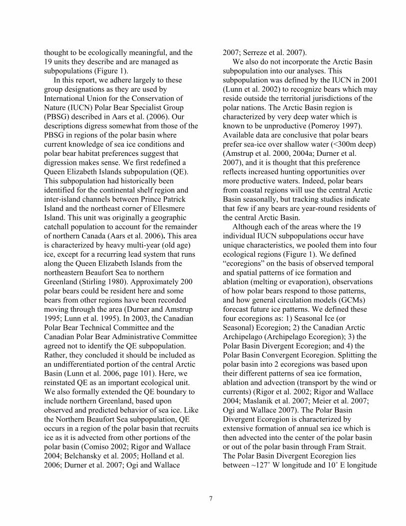
In this report, we adhere largely to these group designations as they are used by International Union for the Conservation of Nature (IUCN) Polar Bear Specialist Group (PBSG) described in Aars et al. (2006). Our descriptions digress somewhat from those of the PBSG in regions of the polar basin where current knowledge of sea ice conditions and polar bear habitat preferences suggest that digression makes sense. We first redefined a Queen Elizabeth Islands subpopulation (QE). This subpopulation had historically been identified for the continental shelf region and inter-island channels between Prince Patrick Island and the northeast corner of Ellesmere Island. This unit was originally a geographic catchall population to account for the remainder of northern Canada (Aars et al. 2006). This area is characterized by heavy multi-year (old age) ice, except for a recurring lead system that runs along the Queen Elizabeth Islands from the northeastern Beaufort Sea to northern Greenland (Stirling 1980). Approximately 200 polar bears could be resident here and some bears from other regions have been recorded moving through the area (Durner and Amstrup 1995; Lunn et al. 1995). In 2003, the Canadian Polar Bear Technical Committee and the Canadian Polar Bear Administrative Committee agreed not to identify the QE subpopulation. Rather, they concluded it should be included as an undifferentiated portion of the central Arctic Basin (Lunn et al. 2006, page 101). Here, we reinstated QE as an important ecological unit. We also formally extended the QE boundary to include northern Greenland, based upon observed and predicted behavior of sea ice. Like the Northern Beaufort Sea subpopulation, QE occurs in a region of the polar basin that recruits ice as it is advected from other portions of the polar basin (Comiso 2002; Rigor and Wallace 2004; Belchansky et al. 2005; Holland et al. 2006; Durner et al. 2007; Ogi and Wallace

2007; Serreze et al. 2007). We also do not incorporate the Arctic Basin

subpopulation into our analyses. This subpopulation was defined by the IUCN in 2001 (Lunn et al. 2002) to recognize bears which may reside outside the territorial jurisdictions of the polar nations. The Arctic Basin region is characterized by very deep water which is known to be unproductive (Pomeroy 1997). Available data are conclusive that polar bears prefer sea-ice over shallow water (<300m deep) (Amstrup et al. 2000, 2004a; Durner et al. 2007), and it is thought that this preference reflects increased hunting opportunities over more productive waters. Indeed, polar bears from coastal regions will use the central Arctic Basin seasonally, but tracking studies indicate that few if any bears are year-round residents of the central Arctic Basin.

Although each of the areas where the 19 individual IUCN subpopulations occur have unique characteristics, we pooled them into four ecological regions (Figure 1). We defined “ecoregions” on the basis of observed temporal and spatial patterns of ice formation and ablation (melting or evaporation), observations of how polar bears respond to those patterns, and how general circulation models (GCMs) forecast future ice patterns. We defined these four ecoregions as: 1) Seasonal Ice (or Seasonal) Ecoregion; 2) the Canadian Arctic Archipelago (Archipelago Ecoregion); 3) the Polar Basin Divergent Ecoregion; and 4) the Polar Basin Convergent Ecoregion. Splitting the polar basin into 2 ecoregions was based upon their different patterns of sea ice formation, ablation and advection (transport by the wind or currents) (Rigor et al. 2002; Rigor and Wallace 2004; Maslanik et al. 2007; Meier et al. 2007; Ogi and Wallace 2007). The Polar Basin Divergent Ecoregion is characterized by extensive formation of annual sea ice which is then advected into the center of the polar basin or out of the polar basin through Fram Strait. The Polar Basin Divergent Ecoregion lies between ~127˚ W longitude and 10˚ E longitude

7

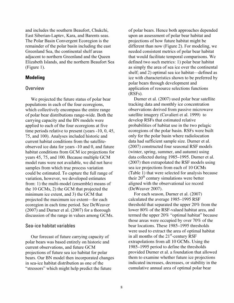
and includes the southern Beaufort, Chukchi, East Siberian-Laptev, Kara, and Barents seas. The Polar Basin Convergent Ecoregion is the remainder of the polar basin including the east Greenland Sea, the continental shelf areas adjacent to northern Greenland and the Queen Elizabeth Islands, and the northern Beaufort Sea (Figure 1).

Modeling

Overview

We projected the future status of polar bear populations in each of the four ecoregions, which collectively encompass the entire range of polar bear distributions range-wide. Both the carrying capacity and the BN models were applied to each of the four ecoregions at five time periods relative to present (years -10, 0, 45, 75, and 100). Analyses included historic and current habitat conditions from the satellite-observed ice data for years -10 and 0, and future habitat conditions from GCM ice projections for years 45, 75, and 100. Because multiple GCM model runs were not available, we did not have samples from which true process variation could be estimated. To capture the full range of variation, however, we developed estimates from: 1) the multi-model (ensemble) means of the 10 GCMs, 2) the GCM that projected the minimum ice extent, and 3) the GCM that projected the maximum ice extent—for each ecoregion in each time period. See DeWeaver (2007) and Durner et al. (2007) for a thorough discussion of the range in values among GCMs.

Sea-ice habitat variables

Our forecast of future carrying capacity of polar bears was based entirely on historic and current observations, and future GCM projections of future sea ice habitat for polar bears. Our BN model then incorporated changes in sea-ice habitat distribution as one of the “stressors” which might help predict the future

of polar bears. Hence both approaches depended upon an assessment of polar bear habitat and projections of how future habitat might be different than now (Figure 2). For modeling, we needed consistent metrics of polar bear habitat that would facilitate temporal comparisons. We defined two such metrics: 1) polar bear habitat as simply the area of sea ice over the continental shelf; and 2) optimal sea ice habitat—defined as ice with characteristics shown to be preferred by polar bears through development and application of resource selections functions (RSFs).

Durner et al. (2007) used polar bear satellite tracking data and monthly ice concentration observations derived from passive microwave satellite imagery (Cavalieri et al. 1999) to develop RSFs that estimated relative probabilities of habitat use in the two pelagic ecoregions of the polar basin. RSFs were built only for the polar basin where radiolocation data had sufficient sample size. Durner et al. (2007) constructed four seasonal RSF models (winter, spring, summer, and autumn) using data collected during 1985–1995. Durner et al. (2007) then extrapolated the RSF models using sea ice projections from each of 10 GCMs (Table 1) that were selected for analysis because their 20th century simulations were better aligned with the observational ice record (DeWeaver 2007).

For each season, Durner et al. (2007) calculated the average 1985–1995 RSF threshold that separated the upper 20% from the lower 80% of the RSF-valued habitat area, and termed the upper 20% “optimal habitat” because those areas were occupied by over 70% of the bear locations. These 1985–1995 thresholds were used to extract the area of optimal habitat in all months of the 21st-century RSF extrapolations from all 10 GCMs. Using the 1985–1995 period to define the thresholds provided Durner et al. a foundation that allowed them to examine whether future ice projections indicated increases, decreases, or stability in the cumulative annual area of optimal polar bear

8

habitat. We used three types of monthly maps from

the Durner et al. (2007) study: 1) Arctic-wide observed sea ice concentrations (1979–2006); 2) Arctic-wide 21st-century sea ice projections by 10 GCMs; and 3) both observed and projected areas of optimal polar bear sea-ice habitat in the two pelagic polar basin ecoregions. From the observed and projected Arctic-wide sea ice concentration maps, we defined and extracted “total available ice habitat” as the annual 12-month sum of sea ice cover over the continental shelves of the two polar basin ecoregions. Ice cover was defined as the aerial extent (km2) of all pixels with ≥50% ice concentration. Since deep water is uncommon in the archipelago and seasonal ice ecoregions, we considered those entire areas to effectively reside over the continental shelf, meaning total ice habitat equated to total ice cover.

Other key sea ice factors of interest included how climate warming may change the duration and distance that ice retreats from the continental shelf regions. Using the observed and projected ice concentration maps, we extracted and summed the annual number of ice-free months in each ecoregion. An ice-free month occurred when the proportion of ice cover (defined above) over the continental shelf dropped below 50% of the total area (again, the archipelago and seasonal ecoregions were considered entirely shelf waters). In other words, we considered the availability of total ice habitat to be compromised if less than half of the continental shelf-waters were ice-covered; hence the respective month was classified as ice-free. Also for each year, for the month of minimum ice extent, we calculated the mean distance from every pixel in an ecoregion to the nearest ice-covered pixel.

We note that expressing changes in sea-ice habitat over time on the basis of annual km2­months tends to minimize the potential effects of sea ice habitat changes projected for the future as well as those that have been observed may have on polar bears. Whereas the yearly

average sea ice extent has declined at a rate of 3.6% per decade, the mean September sea ice extent has declined at a rate of 8.4% per decade (Meier et al. 2007). Further, all GCMs project extensive winter sea ice through the end of the 21st century in most ecoregions (Durner et al. 2007). Therefore the severity of summer periods of food deprivation may be hidden by extensive sea ice in winter. Although polar bears are well adapted to a feast and famine diet (Watts and Hansen 1987), there apparently are limits to their ability to sustain long periods of food deprivation (Regehr et al. 2007b). We recognize that our measure of change in km2-months will be largely insensitive to seasonal effects.

We used the baseline period 1985-1995 to define high-value (optimal) habitat because during this early period of our studies, year-round polar bear movements were less restricted than they were in recent years when sea ice extent was more spatially reduced. The 4 seasonal RSF thresholds, derived from the 1985-1995 period, remained fixed for all time steps in our projections. Thus, when we extracted the area of optimal habitat from RSF maps generated from outputs of GCMs, the threshold values for optimal habitat were those observed in 1985-1995. This approach created a foundation that allowed us to examine whether future ice projections indicated increases, decreases, or stability in the cumulative annual area of optimal polar bear habitat relative to our earliest decade of empirical observations. Inherently, this approach assumes that polar bears in the future will select habitats in the same way they did between 1985-1995 despite seasonal changes in ice extent and distribution.

Other key sea ice factors of interest included how climate warming may produce changes in the duration and distance that ice retreats from the continental shelf regions. Using the observed and projected ice concentration maps, we extracted and summed the annual number of ice-free months in each ecoregion. An ice-free month occurred when the proportion of ice cover (defined above) over the continental shelf

9

dropped below 50% (again, the archipelago and seasonal ecoregions were considered entirely shelf waters). In other words, we considered the availability of total habitat to be compromised if less than half of the shelf-waters were ice-covered; hence the respective month was classified as ice-free. Also for each year, for the month of minimum ice extent, we calculated the mean distance from every pixel in an ecoregion to the nearest sea ice.

Carrying Capacity Model

We developed deterministic calculations of polar bear carrying capacity for each combination of ecoregion, time step, and future minimum, maximum, and multi-model mean GCM projections. Deterministic projections were calculated in Microsoft Excel®. Calculations in the model components are described below.

Habitat amount

First, we compiled the amount of total ice habitat and optimal habitat from the observed sea ice record and from the GCM projections. Specifically, the total annual (Σ 12 months) habitat amount Ht,G was expressed for each of the four ecoregions G and each of the five yearly time periods t as km2-months. For the two polar basin ecoregions (where the RSF study was conducted) we subtracted the optimal habitat area from the estimates of total ice habitat to provide an area of non-optimal habitat.

Change in habitat amount

Despite overall agreement in the direction of change in sea ice extent, there is considerable variability among the GCMs in their simulations of present-day ice extent, as well as disparity with the observed sea ice record (Figure 3). These disparities reflect aspects of GCM model uncertainties that are introduced by many factors (DeWeaver 2007). Disparities of

GCM model predictions with known conditions are not surprising because GCMs are constructed to emulate natural climate variability (Wang et al. 2007). Amounts of ice predicted by the GCM model might not perfectly match amount observed because the observed climate is but one realization of the possible modeled outcomes.

When comparing modeled futures to the present, it would make no sense to project the trends forward from a baseline that “could have been.” Rather, the sensible approach is to use the GCM’s projected rates of habitat change, and apply those rates of change to the actual observed baseline. To this end, we compared the habitat projections at each time step to each model’s “time zero” value, and calculated the percent change in habitat projected by each model relative to itself. This calibrating or normalizing of the estimates of available habitat provided all model results with a common beginning or baseline value in year 0, and took full advantage of the rate of change projected by each model.

We calculated the percent change in habitat amount H at time t with respect to year 0, for each geographic region G, as

(Ht ,G − H 0,G )CH =100* .t ,G H 0,G

One outcome of the calculation of CHt,G was that estimates at year 0 varied among GCM runs. Another outcome of these calculations is that compared to the observed ice extent, the GCM ensemble mean, and most individual models, overestimated ice extent in the study area in both the late-20th century simulations and the early-21st century projections. Furthermore, the recent rate of summer ice decline in the observed data shows a trajectory that is steeper than that of the GCM ensemble mean during the early 21st century. This is a reflection of Stroeve et al.’s (2007) conclusion that Arctic sea ice may be disappearing at a rate that is “faster than forecasted”.

Our normalized CHt,G was further interpreted into categories of direction of change,

10

magnitude of change, and a composite summary of magnitude and direction. Direction was categorized into “contracting” if CHt ,G < 0 or “expanding or stable” ifCHt ,G ≥ 0 . Magnitude

CH > 30.0 ,was categorized into “fast” if t ,G

“moderate” if 15.0 < CH ≤ 30.0 , and “slowt ,G

or none” if < 15.0 . We also make , CHt G

available the specific results for CHt,G so that alternative cutoff values for such categories could be examined if desired. The summary category for habitat change was then based on the habitat change direction category and the magnitude category, as shown in Table 4.

Polar bear densities

We used the most recent estimated population size for each IUCN subpopulation (Aars et al. 2006, Table 5) to calculate polar bear densities. Because estimates were not provided for the East Greenland and Kara Sea subpopulations, we surmised numbers that seemed appropriate based upon the area of habitat and records of harvest where available. Accuracy of the year 0 density estimates is not critical because our goal was to express the relative changes that are likely to occur. In other words, although the numbers of bears in many of the world’s subpopulations are poorly known, our projections of trends in those numbers in this model are valid to the extent that sea ice quantity alone determines polar bear carrying capacity.

We calculated polar bear densities based on observed total ice habitat in each of the four ecoregions. We also calculated polar bear densities based on optimal habitat in each of the two polar basin ecoregions. Following examples in the ecological literature, we refer to the densities estimated from total and optimal habitat as “crude” and “ecological,” respectively (Rinkevich and Gutiérrez 1996; Diller and Thome 1999). We calculated densities as follows. First we tallied present-day (year 0)

polar bear population sizes N0,G in each of the four ecoregions G. We then calculated polar bear densities as

H 0,GDG = ,N0,G

expressed as habitat area (km2-months x 1000) per bear, using the estimates of habitat at year 0 from satellite data. We expressed density in terms of habitat area per bear to avoid the excessively small values that would result from expressing density in terms of bears per area.

We calculated total densities based on total ice habitat area for the Seasonal and Archipelago ecoregions, and we calculated “ecological” and “crude” densities based on optimal habitat and and non-optimal habitat area, respectively, for the Polar Basin Divergent and Convergent ecoregions. Empirical observations indicated that polar bears spend 70% of their time in the portion of the habitat that we called optimal (Durner et al. 2007). We extrapolated this to mean that at any snapshot in time, 70% of the bears in the two polar basin ecoregions were within the identified optimal habitat. We used 70% to estimate an ecological density in the optimal habitat. The remaining 30% of bears in each ecoregion were assigned to the non-optimal habitat to calculate a crude density. All polar bear density calculations were based on year 0 numbers of bears and habitat area, and then applied to other past and future time periods. This assumed that densities are invariant over time in terms of describing potential carrying capacity levels.

Polar bear carrying capacity

We applied year 0 polar bear densities to habitat area in each time period to calculate polar bear carrying capacity Kt,G for each combination of time period t, ecoregion G, and minimum, maximum, and ensemble mean GCM habitat values. The calculation was:

Kt ,G = H t / DG . We used the normalized percent change in habitat to derive values for available habitat at

11

each time step. This assured that our estimates of changes in carrying capacity coincided with the projected estimate of available habitat at each time step. Specifically, we calculated percent change CKt,G in Kt,G from year 0 values, as

(Kt ,G − K0,G )CK = 100 * .t ,G K0,G

This was done for all habitats in the Seasonal Ice and Archipelago ecoregions, and separately for optimal habitat and non-optimal habitat in the Divergent and Convergent ecoregions. We then applied each of the percent change values CKt,G to the estimate of carrying capacity at year 0 K0,G (based on the observed data), to recalculate a normalized value of carrying capacity as

⎛ CKt ,G ⎞

Capacity Change

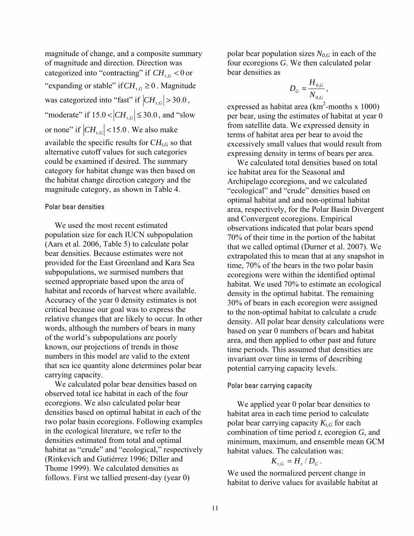
We categorized outcomes of habitat change and carrying capacity change into 4 composite summary categories to describe the status of polar bear populations: enhanced, maintained, decreased, and toward extirpation (Table 2). The composite summary categories express very general classes of carrying capacity levels as compared with current levels, and basically constitute a simple rule set for expressing outcomes in ordinal scale classes. We provide categorical outcomes to depict future polar bear carrying capacity levels in a simple, understandable manner that is relatively insensitive to the accuracy of specific calculations or assumptions. We started these computations with the best estimates available of sea ice habitats and polar bear numbers, and we applied those estimates to the best available

K norm K * 1+= ⎜⎜⎝ 100 ⎟

⎟⎠

.t ,G 0,G

In this way, the values of normalized carrying normcapacity Kt ,G can be compared over time

periods (historic, current, and future) for each of the GCM model run scenarios (minimum, ensemble mean, and maximum) in parity.

Percent change in carrying capacity

We divided the values of change in carrying capacity CKt,G into categories of direction, magnitude, and composite outcomes. Direction was categorized into “decreasing” if CKt ,G < 0 or “stable or increasing” ifCKt ,G ≥ 0 . Magnitude was categorized into “high” if CK > 30.0 , “moderate” ift ,G

15.0 < CK ≤ 30.0 , and “low to none” ift ,G

CK < 15.0. We make available the specifict ,G

results for CKt,G so alternative cutoff values can be examined if desired. The summary categories of carrying capacity change were then derived from the direction and magnitude categories, as shown in Table 6.

Assigning Status Categories Based on Carrying

GCM projections. As mentioned previously, many polar bear

population estimates were crude, and the assumption that polar bear density would not change over time is almost certainly not valid. Collapsing the numerical outcomes of this process into intuitive categories of qualitative results, however, converts the actual numbers to only four general classes. The carrying capacity model is not a demographic model, nor is it an estimation of actual, expected population sizes of polar bears. It is a calculation only of possible carrying capacity and changes thereof, assuming no effects from anthropogenic stressors or environmental factors other than the losses of habitat forecasted by GCMs.

Bayesian Network Population Stressor Model

Our second method of forecasting the status of polar bears in the 21st century involved the development of a prototype Bayesian network (BN) model that accommodates the potential effects of multiple stressors on polar bear populations. Inputs to our BN model included

12

various categories of natural and anthropogenic stressors (Barrett 1981; Anderson et al. 2000), and key environmental factors that affect polar bear populations. Anthropogenic stressors included various human activities that could affect the distribution or abundance of polar bears, such as harvest, pollution, oil and gas development, shipping, direct bear-human interactions, and others. Natural stressors on polar bears included changes in the availability of primary and alternate prey and foraging areas, and occurrence of parasites, disease, and predation (Ramsay and Stirling 1984; Amstrup et al. 2006). Other key environmental factors included projected changes in total ice and optimal habitat, changes in the distance that ice retreats from traditional autumn or winter foraging areas, and changes in the number of months per year that ice is absent in the continental shelf regions. Collectively, the anthropogenic stressors, natural disturbances, and other key environmental factors were structured in a BN model in terms of how they affect polar bear demography and use of foraging areas, and ultimately, how they affect polar bear distribution and abundance.

Below, we provide a general description of BN models and their use in ecological applications. We then describe how we developed the population stressor model for polar bears, how results from the model were analyzed, how we analyzed the model results, and how we conducted sensitivity analyses.

What are Bayesian network models?

A Bayesian network is a graphical model that represents a set of variables that are linked by probabilities1 (Neopolitan 2003; McCann et 1 In BNs, input nodes contain unconditional prior probabilities of their states. The states are assumed to be mutually exclusive and the probabilities sum to one. Prior probabilities are distributed as discontinuous Dirichlet functions in the form of D(x) = lim limcos2n (m!πx) ,

m→∞ n→∞

which is a multivariate, n-state generalization of the two-state Beta distribution with state probabilities being continuous within [0,1]. States S of output nodes contain

al. 2006). BNs are comprised of variable nodes and their links. Nodes can represent correlates or causal variables that affect some outcome of interest, and the links define which specific variables directly affect which other specific variables. A BN defines a causal web with probabilistic links, whereby specifying the conditions of some variables can predict the outcome of some other variables. In this way, BNs constitute what are called influence diagrams (Marcot et al. 2006). BNs provide an efficient way to represent and summarize understanding of a system, and can combine expert knowledge and empirical data into the same modeling structure. Crafting a BN allows one to better understand the relationships and sensitivities among the elements of the causal web, and to provide insights into the workings of the system that otherwise would not have been evident.

Each node in a BN model typically is depicted with two or more mutually exclusive states. BN nodes can represent categorical, ordinal, or continuous variable states or constant (scalar) values. Each node typically has an associated probability table that describes either its prior (unconditional) probabilities of each state for input nodes, or its conditional probabilities of each state for nodes that directly depend on other nodes (see Marcot et al. 2006) for a description of the underlying statistics). BNs are “solved” by specifying the values of input nodes and having the model calculate posterior probabilities of the outcome node(s) through standard “Bayesian learning,” which is the application of Bayes’ theorem (Jensen 2001; see also footnote 1).

Use of Bayesian networks in ecological modeling

posterior probabilities that are calculated conditional upon nodes H that directly affect them, using Bayes

P(H | S)P(S)Theorem, as P(S | H ) = (see Jensen 2001 P(H )

and Marcot 2006 for further explanation of the statistical basis of BNs).

13

BNs are being increasingly used in ecological and natural resource modeling. Examples include use of BNs to model population viability of salmonid fishes (Lee and Rieman 1997), habitat restoration potential for rare wildlife species (Marcot et al. 2001; Wisdom et al. 2002), effects of habitat alteration on populations of native ungulates (McNay et al. 2006), and many other applications (Marcot 2007). BNs are useful for modeling systems where empirical data are lacking, but variable interactions and their uncertainties can be depicted based on expert judgment (Das 2000). They are also particularly useful in efforts to synthesize large amounts of divergent quantitative and qualitative information to answer “what if” kinds of questions. Their ability to examine “what if” questions has led to insights regarding the prognosis for how global warming may impact coral reefs, and the degree to which local management actions may be able to offset some effects of rising temperatures (Wooldridge and Done 2004; Wooldridge et al. 2005).

Structuring the Bayesian network population stressor model for polar bears

Developing a BN model entails depicting the “causal web” of interacting variables (nodes) in an influence diagram (that is, describing the general structure of the model), assigning states to each node, and assigning probabilities to each node that define the conditions under which each state would result. BNs can be built from a combination of empirical data and expert judgment, and can be built using commercially-available modeling shells. We used the modeling shell Netica® (Norsys, Inc.), and followed guidelines for developing BN models developed by Jensen (2001), Cain (2001) and Marcot et al. (2006).

The BN model we developed for polar bears depicted the potential population influences from multiple stressors and environmental conditions that were not captured in the simple carrying capacity model described earlier. Our

BN stressor model was based on the knowledge of one polar bear expert (S. Amstrup) who established the model structure and probability tables according to expected influences among variables. B. Marcot served as a “knowledge engineer” or model engineer, and provided guidance to help structure the expert’s knowledge into an appropriate BN format. An initial list of ecological correlates was compiled by the expert, which were then organized into an influence diagram (Figure 4). Through discussion and questioning, the model engineer guided the expert through several stages to a final structure. The interactive sessions were useful in exploring alternative means of depicting influences among variables, ways to summarize influences into categories of numerical and distribution responses which could be useful to managers, and ways of representing some variables with proxies.

The BN model structure was divided into three kinds of nodes: (1) input nodes that were the anthropogenic stressor or environmental variables and used unconditional probabilities to parameterize their states; (2) summary nodes that collected and summarized effects of multiple input nodes and used conditional probabilities to calculate their states; and (3) output nodes that represented numerical, distribution, and overall population responses to the suite of stressors and environmental conditions. The output nodes used Bayesian learning to calculate posterior probabilities of their final outcome states. Summary nodes in the model served to “gather” and depict the joint influence of several inputs, and constituted what are sometimes called latent variables in the ecological modeling literature (e.g., Bollen 1989). Including latent variable nodes in the BN model was also helpful in establishing probability tables in each node and for characterizing general categories of the input (stressor) nodes. We went through many iterations of the model structure to ensure that it responded to particular input conditions in ways that paralleled responses of polar bear

14

populations which have been observed, or for which there are strong prevailing hypotheses in the biological community.

The overall outcome of our BN model was a statement of the relative probabilities that the population in each ecoregion would be larger than now, same as now, smaller, rare, or extinct. The overall outcome was determined by nodes which summarized the likely numerical and distribution response of polar bears to projected changes in their environment. Responses of polar bears to projected habitat changes and other potential stressors could affect polar bear distribution or polar bear numbers independently in some cases, or they could affect both distribution and numbers simultaneously. Our approach allowed for independent or linked numerical and distributional responses. The factors influencing numerical and distribution responses were, in turn, further defined in terms of more specific human stressor, natural disturbance, or key environmental correlate variables (Figure 5).

Because our purpose was to inform the decision of whether to list polar bears as a threatened species, we designed the summary nodes in the BN model to include four of the five major listing factors used to determine a species’ status according to the Endangered Species Act (U.S. Fish and Wildlife Service 2007). We included summary nodes for Factor A—habitat threats; Factor B—overutilization; Factor C—disease and predation; and Factor E—other natural or man-made factors. We did not include Factor D—inadequacy of existing regulatory mechanisms, because our model focused on ecosystem effects; however, regulatory aspects could be seamlessly added at a future time. Inclusion of these summary nodes recognized the listing factors as important potential stressors and also acknowledged the work done by the FWS during development of the proposal to list polar bears. Structuring the BN model in this way, therefore, helps assure its relevance to the listing process. This structure also anticipates that our BN stressor

model could provide a foundation for a decision model specific to Endangered Species Act listing criteria for this species.

Parameterizing the Bayesian network model

Model input nodes were parameterized with data on ice extent, length of time that ice was projected to be away from identified foraging areas, and the distance of ice retreat from such areas (Table 3). Other nodes incorporated qualitative descriptions of possible states of important environmental correlates. Because we were interested in forecasting changes from current conditions, states of each node were expressed categorically as “compared to now.” That is, they could be in a condition similar to present, they could be in better condition than present, or they could be in worse condition. We set prior probabilities of all input nodes to uniform distributions (complete uncertainty), but before the model was run, we specified the states that seemed most probable (Table 3).

States of environmental correlates were established under each combination of time step, ecoregion, and GCM model outputs. We parameterized the conditional probability tables to assure that node structures were specified in accordance with available polar bear data or expert understanding of data. After initially populating and inspecting the conditional probability tables, we used three different methods to arrive at final values: 1) sensitivity analyses of subparts of the model, 2) solving the model backwards by specifying outcome states and evaluating if the most likely input states that were returned were plausible according to what we know about polar bears now, and 3) running the model (and subparts) forward to ascertain if the summary and outcome nodes responded as expected given the states of the input nodes. These approaches constituted initial calibration of the model to the expert’s knowledge about polar bears and how polar bears are likely to respond to various circumstances. In sum, the goals of this first-generation BN model were to ensure that input

15

conditions matched the current understanding of polar bear biology ecology and responses to observed changes, and that it responded to particular input conditions in ways that paralleled observed responses of polar bear populations.

As fully specified, the BN model included probability tables for each node (Figure 5, Appendix 2, 3). The BN model ultimately consisted of 38 nodes, 44 links, and 1,667 conditional probability values specified by the modelers. The model was solved for each combination of 4 ecoregions, 5 time periods, and 3 future GCM scenarios (ensemble mean, maximum, and minimum). Specifically, for each ecoregion and time period, the three future GCM scenarios were: 1) results projected by the ensemble mean of all 10 GCMs ; 2) results projected by the GCM that forecasted the greatest retention of sea ice; and 3) results projected by the GCM that forecasted the lowest retention of sea ice. Only one data source (the observed record of sea ice) was examined for the historic (1985-1995) and current (1996­2006) time periods. In total, we examined 44 unique combinations. We evaluated correlations among input nodes and between input and output nodes, to assure that colinearity among inputs was not unduly affecting outcome states.

The input data to run each combination were specified by summarizing the respective GCM-derived habitat variables, and by best professional judgment of polar bear expert S. Amstrup (Table 3). Because BN models combine expert judgment and interpretation with quantitative and qualitative empirical information, inputs from multiple experts are usually incorporated into the structure and parameterization of a “final” model. Due to time constraints, however, we were not able to seek and incorporate the input of multiple polar bear experts. Therefore, the model presented here should be viewed as a first-generation prototype. The model will be refined through formally developed processes (see Discussion) at a future time.

Bayesian network model output states

Principal results of the BN model are levels of relative probabilities for the potential states at outcome nodes. In the polar bear BN population stressor model, outcomes of greatest interest were 1) those related to listing factors used by the FWS, 2) the distribution responses, 3) numerical responses, and 4) the overall population response. We evaluated the BN outcomes in terms of the most probable outcome at each of the time steps, and the dispersion of probabilities among all outcomes. Probabilities are presented for each ecoregion and for each of the GCM scenarios we examined. We assessed results from the BN model in the statistical software package SYSTAT 11 (SYSTAT 2004).

We defined our principal outcome nodes (shown in Figure 5) and their possible states as follows:

N o d e C 4 : N u m e r i c a l R e s p o n s e

This node represents the anticipated numerical response of polar bears in an ecoregion based upon the sum total of the identified factors which are likely to have affected numbers of polar bears in any particular area. Such factors include net reproduction as affected by ice habitat conditions, and influences of disease, predation, intentional takes, and human disturbances and stressors. Numerical response outcome states were defined as follows:

• increased density = polar bear density greater than that at Year 0 (year 2000); the density level could be determined empirically to be significantly greater than that at Year 0; density can be expressed in terms of number of polar bears per unit area of optimal habitat (thus expressing "ecological density") or of total (optimal plus suboptimal) habitat (thus expressing "crude density");

• same as now = polar bear density as above

16

but equivalent to the density at Year 0; the density level could be determined empirically to not be different from that at Year 0;

• reduced density = polar bear density less than that at Year 0 (year 2000) but greater than one-half of the density at Year 0; the density level could be determined empirically to be significantly less than that at Year 0 and also significantly greater than one-half of the density at Year 0;

• rare = polar bear density less than half of that at Year 0 (year 2000); the density level could be determined empirically to be significantly less than that one-half that at Year 0;

• absent = polar bears are not demonstrably present; polar bear density is not significantly different than zero.

N o d e C 3 : D i s t r i b u t i o n R e s p o n s e

This is the sum total of ecological and human factors that predict the future distribution of polar bears in the ecoregion. Distribution refers here to the functional response of polar bears (viz., movement and spatial redistribution of bears) to conditions of ice habitat quantity, quality, and temporal distribution; availability of prey and foraging areas; and human disturbances and stressors. Distribution response outcome states were defined as follows:

• same as now = polar bear distribution equivalent to that at Year 0; distribution could be determined empirically to not be different from that at Year 0;

• reduced but resident = a condition in which habitat or prey availability have changed in a way that would likely lead to a significantly reduced spatial distribution (e.g. due to avoidance of a human development, or sea ice is still present in the area but in more limited quantity). Bears

would still occur in the area, but their spatial distribution would be more limited than at Year 0;

• transient visitors = a condition in which habitat or prey availability are seasonally limited or human activities have resulted in a situation where available ice is precluded from use by polar bears on a seasonal basis;

• extirpated = a condition in which habitat or prey availability have declined and human stressors have increased in such a way as to render the area essentially unusable by polar bears, and have lead to a complete or effective dearth of polar bears in the area.

N o d e D 1 : O v e r a l l P o p u l a t i o n O u t c o m e

Overall population outcome refers to the collective influence of both numerical response and distribution response. It incorporates the full suite of effects from all anthropogenic stressors, natural disturbances, and environmental conditions on the expected occurrence and levels of polar bear populations in the ecoregion. Overall population outcome states were defined as follows:

• larger = polar bear populations have a numerical response greater than at present (Year 0) and a distribution response at least the same as at present (that is, able to use available habitat, to relocate if possible and needed, and to withstand anthropogenic stressors);

• same as now = polar bear populations have a numerical response essentially the same as at present (Year 0) and a distribution response at least the same as at present;

• smaller = polar bear populations have a reduced density and a distribution response the same as at present or reduced but resident; or have a density same as at present but occur as reduced but resident or transient visitors;

• rare = polar bears are numerically rare and

17

have a distribution response same as at present, or occur as reduced but resident or transient visitors; or have a reduced density and occur as transient visitors;

• extinct = polar bears are numerically absent or distributionally extirpated.

Here, the “extinct” state refers to conditions of: (1) complete absence of the species (N=0) from an ecoregion; or (2) numbers and distributions below a “quasi-extinction” level, that refers to a non-zero population level at or below which the population is near extinction (Ginzburg et al. 1982; Otway et al. 2004); or (3) functional extinction, that refers to being so scarce as to be near extinction and contributing negligibly to ecosystem processes (Sekercioglu et al. 2004; McConkey and Drake 2006).

Our final BN model was structured to make maximum use of the data and GCM outcomes describing observed and projected changes in the sea ice. Knowledge of polar bears, their dependence on sea ice, and the ways in which sea ice changes have been observed to affect polar bears, were used to populate the conditional probability tables. The BN model also incorporated professional judgment regarding how other ecological and human factors may change if sea ice changes occur as projected. Because our prototype model was parameterized by the best professional judgment of only one polar bear expert, it is reasonable to ask how robust the results might be to input probabilities which could vary among other experts. It also is appropriate to ask whether it is likely that future sea ice change, to which model outcomes are very sensitive, could fall into ranges that would result in qualitatively different outcomes than our BN model projects. Finally, it is appropriate to ask the extent to which model outcomes may be altered by active management of the states of nodes which represent variables which are under human control.

We addressed questions about the ability of changes in human activities to alter the BN output states by fixing inputs which humans

could control and examining differences in the overall outcomes. We evaluated the extent to which sea ice projections would have to differ to make qualitative differences in outcomes by holding all non-ice variables at uniform priors and allowing ice variables only to vary at future time steps. Comparing those results to the range of ice conditions available from GCMs provides a sense of just how much the realized future ice conditions would have to change from those projected to make a difference in population outcomes. Finally, although we cannot second guess how other polar bear experts may recommend parameterizing and structuring the model, comparison of model runs with preset values provides some sense of how much differently the model would have to be parameterized to project patterns qualitatively different than those we observed.

After the BN population stressor model was finalized, we ran overall sensitivity analyses to determine the degree to which each input and summary variable influenced the population outcome variables. We used results of sensitivity analysis to determine the potential effect of each stressor variable on the anticipated polar bear numerical response, distribution response, and overall population outcome.

For discrete and categorical variables, sensitivity was calculated in the modeling shell Netica as the degree of entropy reduction (reduction in the disorder or variation) at one node relative to the information represented in other nodes of the model. That is, the sensitivity tests indicate how much of the variation in the node in question, is explained by each of the other nodes considered. That is, "node X explains this much of the variation in node Y." [See chapter 2 in Burnham and Anderson (1998) for a summary discussion of the entropy concept.] The degree of entropy reduction, I, is the expected reduction in mutual information of an output variable Q with q states due to a finding of an input variable F with f states. For discrete variables, I is measured in terms of

18

information bits and is calculated as:

P(q, f ) log2[P(q, f )]I = H (Q) − H (Q | F ) =∑ ∑q f P(q)P( f )

where H(Q) is the entropy of Q before new findings are applied to input node F, and H(Q|F) is the entropy of Q after new findings are applied to F. In Netica, entropy reduction is also termed mutual information.

For continuous variables, sensitivity is calculated as variance reduction VR, which is the expected reduction in variation, V(Q), of the expected real value of the output variable Q due to the value of input variable F, and is calculated as

VR = V (Q) −V (Q | F ) , where V (Q) =∑q

P(q)[X − E(Q)]2 ,q

V (Q | F ) =∑ P(q | f )[X q − E(Q | f )]2 , and q

E(Q) P(q)X ,=∑q q

and where Xq is the numeric real value corresponding to state q, E(Q) is the expected real value of Q before new findings are applied, E(Q|F) is the expected real value of Q after new findings f are applied to F, and V(Q) is the variance in the real value of Q before any new findings (Marcot et al. 2006)

The greater the values of I or VR, the greater is the influence of input variable F on output variable Q. In this way, we were able to assign an order to the potential influence of each input and summary node on the population outcome nodes, and thereby describe the overall sensitivity structure of the model.

Results

In this section we first present the projection of carrying capacities for polar bears in each ecoregion based on a presumed linear relationship between sea ice extent and polar bear numbers. That projection, which does not include seasonal changes in the sea ice, or other

factors which could be population stressors, provides an upper bound on polar bear populations that could be supported by sea ice habitat available in the future. We next present projections based on the BN population stressor model. Because it incorporated many of the factors not included in the projection of carrying capacity, it provides a more thorough assessment of the future of polar bears in each ecoregion.

Forecasted 21st Century Polar Bear Carrying Capacity

Habitat area and change

Total habitat area, expressed as the annual sum of km2-months of sea ice extent, was projected by the GCM models to be reduced (Figure 3) from present-day conditions, at each time step in each ecoregion and for all ecoregions combined (global). Proportional declines in available total habitat ranged from relatively modest (less than 15% decline from present) at year 45 in the Seasonal Ice Ecoregion, to large (more than 47% decline) by year 100 in the Polar Basin Divergent Ecoregion (Table 4, Figures 6, 7). For all combinations of time steps, GCM runs, and ecoregions, both total and optimal habitat were projected to be less abundant than present amounts (Table 4, Figures 6, 7). Globally, projected habitat declines were 24%, 18%, and 15% for the minimum, mean, and maximum GCM model inputs, respectively, by year 45. Equivalent global values at year 100 were 40%, 32%, and 23% for minimum, mean, and maximum ice projections, respectively. Using the satellite observed sea ice record, total habitat area during the previous decade (year -10) varied among ecoregions and was between 3% and 17% more abundant than at present. Globally, total habitat in the last decade was 7% more abundant than it is now (Figures 6, 7).

19

Polar bear carrying capacity

Current estimated polar bear densities ranged from a high of 0.923*103 km2-months per bear in the Polar Basin Convergent Ecoregion, to a low of 7.695*103 km2-months per bear in the non-optimal portion of the Polar Basin Divergent Ecoregion (Table 5). Estimates of polar bear carrying capacity (Kt,G) based upon these densities, as well as percent change in carrying capacity from present (CKt,G), and

normcarrying capacity normalized to present ( Kt ,G ), are presented in Table 6, and Figures 8 and 9. As with total habitat, total historical carrying capacity (year -10) ranged from 3 to 17% greater than at present in the Archipelago and Seasonal Ice Ecoregions, respectively, and 8% globally (Figure 9).

In the Seasonal Ice Ecoregion, we projected total carrying capacity to decline 7-10% from present levels by year 45, 21-32% by year 75, and 22-32% by year 100 (ranges of percentages depending on habitat amount predicted by the GCM maximum and GCM minimum results, respectively; Table 6, Figures 8, 9). In the Archipelago Ecoregion, we projected total carrying capacity to decline 3-14% from present levels by year 45, 18-21% by year 75, and 21­24% by year 100. In the Polar Basin Divergent Ecoregion, total carrying capacity dropped 19­35% from present levels by year 45, 29-43% by year 75, and 23-48% by year 100. In the Polar Basin Convergent Ecoregion, total carrying capacity ranged from -24% to +4% of present levels by year 45, and dropped 8-28% by year 75, and 3-31% by year 100.

For the two polar basin ecoregions, model data also were available on amount of optimal habitat and carrying capacity within optimal habitat (Tables 2,4; Figs. 7,8). In the Polar Basin Divergent Ecoregion, we projected carrying capacity of optimal habitat to drop 17­36% at year 45, 31-45% at year 75, and 21-49% at year 100, again because of relatively greater loss of optimal habitat. Conversely, the Polar Basin Convergent Ecoregion appeared to

largely maintain non-optimal habitat, although there was considerable variation among models and time periods. The increasing proportion of non-optimal habitat along with corresponding increase in its carrying capacity (by as much as 49% by year 45 under the GCM maximum scenario), however, was insufficient to prevent overall declines in total carrying capacity, in most model runs. This was caused by strong declines in the carrying capacity of optimal habitat in latter years of the projections. Nonetheless, projected habitat losses in the Polar Basin Convergent Ecoregion were more modest and more variable among all model runs than in the Polar Basin Divergent Ecoregion. The optimal habitat-based carrying capacity showed declines ranging up to 31% loss by year 100, with no gains in any time period. In all ecoregions, trends consistently suggested moderate to large decreases in total carrying capacity by year 75, and moderate decreases in all ecoregions beginning in year 45. Globally, total carrying capacity across all ecoregions was projected to drop 10-22% from present levels by year 45, 22-32% from present levels by year 75, and 20-37% from present levels by year 100 (Figure 9).

Overall, total carrying capacity was projected to decrease at all time steps we examined in the 21st century. Models which projected minimal ice extent projected trends toward extirpation of bears from the Polar Basin Divergent Ecoregion by year 45 and from the Seasonal Ecoregion by year 75. Under ensemble mean ice conditions, we projected likely extirpation of bears in the Polar Basin Divergent Ecoregion by year 75 and in the Polar Basin Convergent Ecoregion by year 100 (Table 7).

Bayesian Network Model Forecast of the 21st Century Status of Polar Bears

Overall outcomes projected by our BN model which included the consideration of population stressors in addition to sea ice area effects were ranked according to relative

20

probability in Table 8. In all but the Archipelago Ecoregion, the dominant outcome state was "extinct" at all future time periods (Figure 10). Probabilities of the “extinct” state for future time periods varied from a low of 8% in the Archipelago Ecoregion at year 45 under the GCM maximum scenario, to a high of 87% in the Polar Basin Divergent Ecoregion at year 45 under the GCM minimum ice scenario (Table 8, Figure 11).

In the Archipelago Ecoregion, a smaller population was the dominant outcome at year 45 under all GCM scenarios, and at year 75 only for the GCM maximum scenario. Even in the Archipelago Ecoregion, “extinct” was sometimes the dominant outcome for other combinations of time periods and GCM modeling scenarios (Figure 10).

In the Seasonal and Polar Basin Divergent ecoregions, "extinct" was by far the most dominant outcome with very low probabilities forecast for all other outcome states in all time periods. The low probability afforded to outcome states other than extinct suggested a clear trend in these ecoregions toward probable extirpation by mid century. At year 45 in the Polar Basin Convergent Ecoregion, and at all future time steps in the Archipelago Ecoregion, considerable probability fell into outcome states other than extinct (Figure 10). Even when extinct was the most probable outcome, other outcomes sometimes had large non-zero probabilities.

The general trends of the overall population outcome (node D1) from the BN model (Table 8, Figure 10 and 11) can be viewed as follows. In each ecoregion, the polar bear population was very likely larger or at least incurred a far lower likelihood of multiple stressors in the past than compared to present. In the future, however, multiple stressors will likely play important and deleterious roles on all polar bear populations, even starting at year 45, and generally increase in their effect through year 100. Effects of multiple stressors appear to have a composite influence on the overall populations at more or

less the same intensities regardless of the GCM modeling scenario (Table 8).

When the overall population outcome is broken down into its component influences, some further differences among ecoregions, time steps, and GCM modeling scenarios become apparent. For instance, there seems to be a greater adverse influence from future conditions on polar bear distribution response (node C3) than on polar bear numerical response (node C4) (Table 9). In part this is because of salient adverse future outcomes of habitat threats (node F2; Table 10) and foraging habitat distribution, especially in the Seasonal and Polar Basin Divergent ecoregions (Table 11). The BN model also represents worsening future conditions of natural disturbances including disease and predation (Table 12) and overall adverse influences on reproduction and vital rates (Table 13).

Sensitivity Structure of the Bayesian Network Population Stressor Model

We conducted 10 tests on the BN population stressor model to determine its sensitivity structure (Appendix 1). In general, the BN model seemed well balanced in terms of its underlying probability tables, in that sensitivity of the final outcome variable (node D1, overall population outcome) was distributed among all arms of the model. In other words, no single input variable or small clique of input variables unduly dominated the overall population outcome (see Appendix 1, sensitivity test 1).

Some 91% of the variation in overall population outcome (node D1) was explained by the top six variables (Appendix 1, Figure 12). Four of those top six variables were sea ice related, including our quantitative data on spatiotemporal change. The ecoregion of consideration and the level of intentional takes rounded-out the top six variables with influence on overall population outcome. In essence, ecoregion also is a habitat variable because ecoregions were specified on the basis of their

21

differences in sea ice. In that context, 5 of the top six variables explaining variation in overall outcome related to the nature of the sea ice.

The primary importance of sea ice change and lesser but complementary importance of anthropogenic stressors carried through to determinations of which FWS listing factors explained the most variation in overall outcome. Relative to the FWS listing factors, overall population outcome was by far most influenced by stressors related to Factor A (habitat threats). Influences from Factor B (overutilization), Factor E (other natural or man-made factors), and Factor C (disease and predation) provided progressively less influence (Appendix 1, sensitivity test 2).

Subsections of the BN model (“submodels”) also were tested for sensitivity (Appendix 1, sensitivity tests 5-10). Notable among these tests was that foraging habitat value (node A, a composite “latent variable” created to summarize effects of several key environmental factors), was most sensitive to foraging habitat character, which is a subjective assessment of the quality of sea ice used for foraging by polar bears (Appendix 1, sensitivity test 8). Foraging habitat character (node S1) was included in the BN model to reflect observations that recent changes in the sea ice have included increased roughness and rafting among ice floes that are thought to reduce foraging effectiveness of polar bears (Stirling et al. 2008).

Discussion

We begin this section with a discussion of uncertainty as it pertains to our objectives and our outcomes. We follow a treatment of general uncertainty with a discussion of our carrying capacity model outcomes. Then, we describe the state of development in our BN polar bear population stressor model. That description includes identification of caveats regarding the current stage of development of the model and next steps necessary to address those caveats. Finally, we assess the BN model outcomes with

regard to existing knowledge about polar bears and with respect to observed and projected changes in their sea ice habitats on which they depend.

Types and Implications of Uncertainty

Analyses in this report contain three main categories of uncertainty: (1) uncertainty in our understandings of the biological, ecological, and climatological systems; (2) uncertainty in the representation of those understandings in models and statistical descriptions; and (3) uncertainty in model predictions.

First, uncertainty in our understanding of complex ecosystems is virtually inevitable, particularly for one as extensive and remote as the circumpolar Arctic. We have however, incorporated a broad sweep of knowledge regarding polar bears and their environment which is available from published literature, from other reports informing the listing process, and from expert interpretations of that available information.

How to best represent our understanding of the system in models can be structured in various ways. In this report, we captured and represented expert understanding of polar bear habitats and populations in a manner that can be reviewed, tested, verified, calibrated, and amended as appropriate. We have attempted to open the "black box" so to speak, and fully expose all formulas and probabilities used in the polar bear carrying capacity and the BN population stressor models. We also used sensitivity testing to help convey the reliability of BN model depictions (Johnson and Gillingham 2004) (Appendix 1). After BN models of this type are modified through peer review, or revised with knowledge from more than one expert, any variation in resulting models can represent the divergence (or convergence) of expertise and judgment among multiple specialists.

Also included in the second category of uncertainty are uncertainties associated with

22

statistical estimation of parameters such as the extent of sea ice or size of polar bear populations. Statistical estimation typically includes systematic measurement error and random error, for example, as partitioned in general linear models and as may arise in classification functions such as assigning categories to map areas. In this case, we have minimal opportunity to address these estimation errors. The sea ice parameters we used in our polar bear models were derived from GCM outputs, which possess their own wide margins of uncertainty (DeWeaver 2007). Hence, the magnitude and distribution of errors associated with our sea ice parameters were unknown.

To compensate for these unknowns, we accommodated a broad range of sea ice uncertainties by analyzing the 10-member ensemble GCM mean, as well as the minimum and maximum GCM ice forecasts. In the case of polar bear population estimates, many are known so poorly that the best we have are educated guesses. Pooling subpopulations where numbers are merely guesses, with those where precise estimates are available, to gain a range-wide perspective prevents meaningful specific calculation and incorporation of error terms. We recognize that difficulty, but because our projections are expressed in the context of a comparison to present conditions, we largely avoid the issue. That is, whatever the population size is now, the future size is expressed relative to that and all errors are carried forward.

The third category of uncertainty pertains to model predictions. Predictions from models of species abundance and distribution can be subject to at least three sources of error: error due to spatial autocorrelation, dispersal and movement of organisms, and biotic and environmental interactions (Guisan et al. 2006). We addressed these error sources in the following ways. The estimates of ice habitat area were derived separately for each ecoregion from the GCM models because the ecoregions behave independently in terms of sea ice advection. The BN population stressor model

accounted explicitly for potential movement of polar bears (e.g., use of alternative foraging areas) and for biotic and environmental interactions (as expressed in the conditional probability tables; see Appendix 3).

Deterministic models, such as the spreadsheet carrying capacity model, present calculations and predictions essentially as point values with no variance or error. In the absence of empirical measures of variation, one could presume a Gaussian error distribution around such calculated predictions. However, in our polar bear carrying capacity model there was no means of determining the magnitude of that error (nor did we have empirical estimates of variation surrounding polar bear population sizes by ecoregion). Hence, we did not attempt to estimate error levels for the carrying capacity calculations, although we acknowledge there is uncertainty surrounding those values.

Probabilistic or stochastic models, such as the BN population stressor model, can inherently display results as probabilities of various states or potential outcomes. The spread and magnitude of probability values across the outcome states in the BN model reflect the combination of uncertainties in states across all other variables, as reflected in each of their conditional probability tables. More sophisticated means of estimating variance of the probabilities of outcome states can also be undertaken (e.g. calculating their standard deviation and standard error from bootstrapping random subsets of the input values (Guisan and Zimmermann 2000) or from random subsets of simulated output cases). These additional steps are laborious, however, and better undertaken after the BN model has been through additional peer review and established as at least a beta level model (see below).

The spread of probabilities among the BN outcome states is itself an expression of uncertainty and important information for the decision-maker who may wish to weigh alternative outcomes in a risk assessment. When predictions result in high probability of one

23

population outcome state and low to zero probabilities of all other states, there is low overall uncertainty of predicted results, presuming that the other categories of uncertainty (in our understanding of the system and our representation of that understanding in the modeling) are taken into account. In some cases, however, the BN model predicts nearly equivalent probabilities of more than one population outcome state. In these cases, uncertainty of the outcomes is greater, and the decision-maker may wish to weigh the probabilities according to his or her risk attitude and decision criteria.

Finally, model uncertainty also entails addressing model credibility, acceptability, and appropriateness of the model structure. We made every effort to ensure that the model structure was appropriate and credible, and that the inputs were parameterized according to best available knowledge on polar bears and their environment. We have explored the logic and structure of our BN model through sensitivity analyses, running the model backwards from particular states to see if it returns us to the appropriate starting point, and performing particular “what if” experiments (e.g., by fixing values in some nodes and watching how values at other nodes respond). We are as confident as we can be at this point in model development that the model is performing correctly and providing outcomes that can be useful in qualitatively forecasting the potential future status of polar bears. Because the model has been structured and parameterized by only one polar bear expert, however, there are additional criteria of model validation that must be addressed through subsequent peer review and model revision (Marcot et al. 1983; Marcot 1990, 2006).

Forecasted 21st Century Polar Bear Carrying Capacity

All 10 of the GCMs we analyzed project a downward trend in sea ice extent in the 21st

century (DeWeaver 2007). Those declines are paralleled by projected declines in both total and optimal polar bear habitat at all time steps (Figure 3, Durner et al. 2007). The wide range of outcomes in each region and time period represents the spread of values from the GCM model runs, even when normalized to present-day conditions. Despite the range of outcomes, however, declines in available polar bear habitat translate to lower carrying capacity for polar bears in all ecoregions at all future time steps (Figures 8, 9).

Our projected rates of decline in habitat and polar bear carrying capacity are generally slower than rates that have actually been observed during the past two decades. This is most notable in the Seasonal Ice Ecoregion where the rate of sea ice decline has been among the most profound of any in the Arctic (Meier et al. 2007). Yet, data derived from GCM forecasts appeared to suggest slow rates of future declines in the Seasonal Ecoregion (Figures 7, 9). This inconsistency in the Seasonal Ecoregion is apparently caused, at least in part, by some GCM projections that consistently put large amounts of sea ice over the continental shelf habitats in Davis Strait and Baffin Bay. Whereas the analyses of GCM outputs suggest decreases of 15-45% in sea ice cover in Hudson Bay through the next century, the same models forecast more ice remaining over the continental shelves of Davis Strait than was actually observed in that region between 1996 and 2006. Similarly, GCMs predict only a 7% decrease of sea ice in Baffin Bay by 2100. In contrast, satellite observations verify that Baffin Bay sea ice extent declined over 10% between the 1985-1995 period and the 1996­2006 period. Between those same periods the sea ice extent over the continental shelves of Davis Strait declined 51%.

The rapid rate of observed ice loss in the Seasonal Ice Ecoregion suggests that modeled persistence of ice there in the future is probably not realistic. This concept is corroborated by observations that show this ecoregion has seen

24

as much warming as almost any other location in the Arctic (Comiso and Parkinson 2004). If anything, sea ice declines in the Seasonal Ice Ecoregion are likely to be hastened in the future if temperatures continue to increase (Stirling and Parkinson 2006). Therefore, our projected gradual declines in polar bear carrying capacity in the Seasonal Ice Ecoregion are probably optimistic and biased on the high side.

In most other regions, the differences between observed and projected ice loss are smaller, but still variable. For example, the Polar Basin Divergent Ecoregion has seen a 4.5% loss in total habitat during the observational period. The ensemble mean forecast for ice loss in the ecoregion is 9% during the next 50 years and 26% by the end of the century. In contrast, individual IUCN subpopulation areas within the Polar Basin Divergent Ecoregion were forecast to have up to 95% decline in ice habitat. Nonetheless, the range of values in our projections appears to capture a general trend of large ice losses, large losses of optimal habitat, and large losses of carrying capacity for polar bears in the Polar Basin Divergent Ecoregion.

In contrast to the Seasonal and Polar Basin Divergent Ecoregions, we forecast more modest changes in habitat and polar bear carrying capacity for the Archipelago and Polar Basin Convergent Ecoregions. These more modest habitat losses appear consistent with modest losses during the observational period and with the forecasted changes in the individual IUCN subpopulation areas. These results parallel recent sea ice observations that show minimal declines in these ecoregions (Meier et al. 2007).

Although the pattern of projected carrying capacity varied greatly among regions, the bottom line was for an overall range-wide decline in polar bear carrying capacity of between 10% and 22% by year 45 and between 20% and 37% by year 100 (Table 6, Figure 9). The carrying capacity model forecasted that polar bears could be extirpated from the Polar Basin Divergent Ecoregion as early as year 45.

Projections from this modeling approach are deterministic projections based on current estimated densities of polar bears. They depend upon the extent of the sea ice and optimal sea ice habitat only and do not account for possible changes in relative carrying capacity as the amount of ice changes. For example, if thinner ice for shorter periods of time results in more insolation penetrating the water column and greater productivity of the remaining ice habitat, carrying capacity per unit area may rise. If on the other hand, declines in the areal extent of the under ice (epontic) community, which currently provides much of the productivity in Arctic seas (Sakshaug 2004) is not compensated by benefits of increased insolation, carrying capacity could decline. More open water in summer means more new ice forming in winter, which could increase brine expulsion (Fisher et al. 2006) with a variety of potential effects on epontic productivity. Even if overall productivity increases, if the character of the sea ice is dramatically different, polar bears may be ill-suited to forage there. The carrying capacity model cannot accommodate such scenarios, nor can it account for adverse effects of stressors other than changes in sea ice extent.

Just as the carrying capacity model cannot capture possible changes in marine productivity, it also cannot capture the importance of seasonal variation in sea ice. Durner et al. (2007) illustrated that although the annual trend in km2-months of optimal habitat is useful for comparing large scale patterns, it overlooks the importance of seasonal variation. Whereas the GCM ensemble forecasts a polar basin-wide decline of 36% in annually available optimal habitat, it suggests declines of nearly 80% during summer (Figure 13). This reflects the fact that all GCMs forecast sea ice will continue to cover the whole polar basin during the winter through most of the 21st century. So, the realized future changes in ice habitats are seasonally dependent. This is important because seasonal fluctuations in sea ice cover include changes in the location of sea ice as

25

well as its total quantity. Among the most substantive spatial changes

is the retreat of ice from the continental shelves of the polar basin (Comiso 2002; Rigor and Wallace 2004; Belchansky et al. 2005; Holland et al. 2006; Durner et al. 2007; Ogi and Wallace 2007; Serreze et al. 2007). Hence, not only is the sea ice declining in this region on an annual basis, there will be little or no ice in the region at all in summer. The continental shelves of the polar basin are far more productive than the deep polar basin regions offshore (Pomeroy 1997; Sakshaug 2004). Observations show that polar bears spend most of their time foraging on sea-ice over shallow water (<300m deep) (Amstrup et al. 2000, 2004a; Durner et al. 2007), where it is thought that they hunt most effectively (Stirling et al. 1981; Stirling 1997). Seasonal absence of sea ice from the shelf regions of the polar basin, therefore, can be expected to have a greater effect on foraging than the annual changes in sea ice quantity might suggest.

The length of time that ice is absent from important foraging areas is another variable that our carrying capacity model cannot accommodate. Polar bears are well adapted to survive periods of food deprivation. Those adaptations that have allowed them to successfully exploit the Seasonal Ice ecoregion (Watts and Hansen 1987). There, marine productivity is high enough that polar bears can gain sufficient mass before the ice melts to sustain a long summer and autumn fast.

The polar basin, in contrast to most of the seasonal ice regions, is relatively low in productivity (Sakshaug 2004). Whereas polar bears in the Seasonal Ecoregion reach peak body weights before the ice melts in summer; polar bears in the polar basin do not reach peak body weight until late autumn or early winter (Durner and Amstrup 1996). This suggests they have a different temporal pattern of weight gain to compensate for the relatively low productivity of the polar basin seas. Polar bears in the polar basin simply need more time to

reach the weight necessary to survive the winter. Another indication of the low productivity, with which polar bears contend in the polar basin, is the observation that polar bears in the polar basin reach sexual maturity later in life than they do in other portions of their range. In the polar basin, polar bears produce their first young at age six. This is in contrast to much of the Canadian Arctic where they breed for the first time at age 4 and produce their first cubs at 5 years of age (Stirling et al. 1977, 1980, 1984; Ramsay and Stirling 1982, 1988; Furnell and Schweinsburg 1984; Amstrup 2003). Polar basin bears, therefore, may not be able to accommodate extended seasonal absence of sea ice from their preferred foraging habitats. Indeed, recent analyses suggest that the length of time that ice is absent from continental shelf foraging areas may be related to certain measures of physical stature and cub survival (Rode et al. 2007) as well as a predictor of survival (Hunter et al. 2007; Regehr et al. 2007a) in polar bears of the Beaufort Sea.

As noted earlier, most GCMs project that ice will return to much of the Arctic in winter, even late in the century. This fact is reflected in the relatively modest changes in sea ice extent we report on an annual basis--the seasonal absence is to great extent masked by the recurrence of ice in winter. Our carrying capacity model therefore does not account of these seasonal aspects of sea ice change. The impact of periods of food deprivation which are too long for polar bears to accommodate is just not represented by the changes in sea ice extent expressed as km2­months. This shortcoming is another reason that the carrying capacity model likely underestimates the effects future sea ice change will have on polar bears.

Even with all of the caveats that accompany the carrying capacity modeling, however, the conclusion that polar bear populations will face major declines over large portions of their current range seems sound if the sea ice declines as predicted. The carrying capacity model

26

suggests the greatest declines will be in the Polar Basin Divergent Ecoregion where extirpation could occur by mid-century and seems very likely by late-century. Using the recent observational sea ice record to qualify the carrying capacity projections for the Seasonal Ice Ecoregion, it seems more likely that extirpation will occur there despite the fact that that outcome was forecasted from only the GCM minimum ice projections. The carrying capacity model further suggests that polar bears, in reduced numbers, are likely to persist in the Polar Basin Convergent Ecoregion and the Archipelago Ecoregion through the end of the 21st century.

Bayesian Network Model Forecast of the 21st Century Status of Polar Bears

Next steps in the BN model development

Before we discuss outcomes of our BN model, we provide a detailed description of its current state of development and the next steps in that development. Because BN models combine expert judgment and interpretation with quantitative and qualitative empirical information, inputs from multiple experts (if available) are necessary before a model can be considered final. Due to time constraints, however, we were not able to seek and incorporate the input of multiple polar bear experts into our BN model. Therefore, the model presented here should be viewed as a first-generation “alpha” level prototype (Marcot et al. 2006). It captures and depicts judgment of one subject matter expert. It is therefore, in a general sense, an expert system (Martin et al. 2005; McCann et al. 2006), but still must be vetted through other polar bear experts.

The next model development steps, including the vetting necessary to advance development of our prototype “alpha” level model, have been described in detail by (Marcot et al. 2006), and include:

• further peer review of the alpha model by

other subject-matter experts;

• reconciliation of the peer reviews by the initial expert, and updating the model to a beta level that incorporates the reviews;

• testing of the beta level model for accuracy with existing data (e.g., determining if it matches historic or current known conditions); and

• updating the model to the next “gamma” level with existing data, or even to a delta level through incorporation of additional validation data from new field work or new analyses if available.

Throughout this process, sensitivity testing can be used to verify model performance and structure. This framework has been used successfully for developing a number of BN models of rare species of plants and animals (Marcot et al. 2001, 2006; Raphael et al. 2001; Marcot 2006).

The next step in the development process of the polar bear BN population stressor model is the review of the current prototype by peers--in this case by other polar bear experts. The process of review of the model by other polar bear experts is akin to the peer review of a manuscript sent to a journal. The initial model engineer can serve as an "editor" to present the alpha-level model to one or more other experts in the field; to elicit and compile their critique and comments on overall model structure (the variable used and their connections) and probabilities; and then to return to the initial expert with the reviews. The review by peers could result in revision of the alpha-level model, producing a variant(s) of the model that more adequately represents the reviewer's own expert knowledge and judgment. The initial expert develops a "reconciliation" of the reviews that annotates how each review comment was addressed in modifying the model (or not). The result is modification, or perhaps retention, of the alpha-level model structure, to produce the beta-level model which incorporates inputs from more than one expert.

27

Model variants that may have emerged in the review process would represent the range of expert opinions and experiences, and this range could be important information for decision-making.

Further advancing of the model beyond a beta-level, depends on whether new analysis results or new empirical data are available. Because BN models are best viewed as working tools useful to project outcomes, and to guide monitoring and data collection this becomes an interactive process. The model sensitivities can indicate which monitoring efforts will provide the information most useful to future decisions. The full model or portions of the model can be tested for performance against new data generated by that monitoring. The model is then validated and updated. This advantage of the BN modeling approach which allows new field data or new empirical observations to be incorporated into the model as they come along, allows for continual tests of model performance and provide new inputs which can be, in turn, used to improve model performance. Every new piece or data and new relevant observation allows further refinement of the performance of the model (Marcot 2006).

Because these additional steps in development of our prototype model have not yet been completed, it is important to view probabilities of outcome states in terms of their general direction and overall magnitudes rather than focusing on the exact numerical probabilities of the outcomes. When predictions result in high probability of one population outcome state and low or zero probabilities of all other states, there is low overall uncertainty of predicted results. When projected probabilities of various states are more equally distributed, however, careful consideration should be given to large nonzero probabilities representing particular outcomes even if those probabilities are not the largest. Consistency of pattern among scenarios (e.g., different GCM runs) also is important to note. If the most probable outcome has a much higher probability

than all of the other states, and if the pattern across time frames and GCM models is consistent, it is most likely important to note that outcome and pattern. If on the other hand, probabilities are more uniformly spread among different states, and if the pattern varies among scenarios, the importance of the most probable outcome may not be as great. This approach takes advantage of the information available from the model while recognizing that it is still in development. It also conforms to the concept of viewing the model as a tool describing relative probabilistic relationships among major levels of population response under multiple stressors.

BN model projected outcomes

In the BN model, for each scenario run, the spread of population outcome probabilities (or at least non-zero possibilities) represented how individual uncertainties propagate and compound across multiple stressors. Beyond year 45, “extinct” was the most probable state into which polar bear populations in all ecoregions moved, except those in the Archipelago Ecoregion (Figure 10, Table 8). Distribution changes driven by changes in the sea ice appeared to be a major factor leading to these predictions. The sea ice extents of the Polar Basin Divergent Ecoregion and Seasonal Ice Ecoregion have declined more rapidly than other places in the Arctic (Meier et al. 2007). The loss of sea ice habitats in the Polar Basin Divergent Ecoregion is projected to continue, and possibly to accelerate (Holland et al. 2006; Stroeve et al. 2007; Durner et al. 2007). Because polar bears are tied to the sea ice for obtaining food, major changes in the quantity of and distribution of sea ice must result in similar changes in polar bear distribution. In this sense, our carrying capacity model incorporates an element of foraging efficiency, even though it cannot directly account for other potential stressors per se.

The BN model suggested that polar bear

28

populations in the Seasonal Ice Ecoregion moved into the extinct category rapidly in contrast to outcomes projected by the carrying capacity model. This may have been because the BN model incorporated aspects of the spatiotemporal distribution of the sea ice that are consistent with recent analyses (Hunter et al. 2007; Regehr et al. 2007a) suggesting that long periods without ice habitats over continental shelf foraging areas may be associated with decreased survival of polar bears. In addition to variables representing the availability of sea ice over the continental shelves, our BN model incorporated other potential stressors not included in our projection of carrying capacity which could have resulted in the different forecasts for the Seasonal Ice Ecoregion. The BN model projection for the Seasonal Ice Ecoregion also seems more in line with the observational record (Stirling and Parkinson 2006; Meier et al. 2007) and provides added cause for reconsideration of the results of the carrying capacity model in the Seasonal Ice Ecoregion.

Overall outcomes projected for polar bears appeared to be driven more by distributional effects than numerical effects. The most probable outcomes for Factor A (Habitat Threats) of the Proposal to list polar bears as a threatened species were “major restriction” (Table 10). Numerical responses of polar bears to future circumstances were forecast to be more modest than changes in distribution. In all regions, reduced density was the most probable outcome (Table 9). One way to interpret that outcome may be that where habitat remains, polar bears will remain even if in reduced numbers. This is consistent with our BN model results suggesting that polar bear populations may remain in the Archipelago Ecoregion at least into the middle of the 21st century. Corresponding with our carrying capacity projection, declines in distribution and number are likely to be faster and more profound in the Polar Basin Divergent Ecoregion and the Seasonal Ecoregion than elsewhere.

Importantly, our results suggest that a core of polar bear habitat and some number of polar bears is likely to persist in and around the Archipelago Ecoregion at least into mid century.

Sensitivity analyses

Sensitivity analyses offer an opportunity to interpret model outcomes at every level. The overall population outcome was most sensitive to change in habitat quantity (node B) and temporal habitat availability (node C). The other major habitat variable, change in distance between ice and the continental shelf (node N) was the 6th most influential factor on the overall population outcome. Change in distance between ice and the continental shelf may have been ranked much lower than the other two quantitative sea ice variables because it was a measurement which only applied to the two polar basin ecoregions. This variable was not calculated in the Archipelago or Seasonal Ice Ecoregions because waters there are all (or essentially all) over the continental shelf. Nonetheless, the combination of these three habitat variables explained 64% of the uncertainty in the overall population outcome. Ecoregion was the 3rd most influential node on overall outcome. We constructed the model recognizing that the four ecoregions differed in the nature of the sea ice which occurred there and in how polar bears utilize that ice. The fact that ecoregion explained 15% of the variation in overall population outcome is further evidence of the importance of sea ice habitat and its regional differences, to polar bear responses to projected habitat change. This is an important result helpful in understanding that, for example, polar bears appear to be facing much greater restriction in the Polar Basin Divergent and Seasonal Ice ecoregions than they do elsewhere.

Another habitat variable, “sea ice character” (node S1), was ranked 5th among variables having influence on the overall population

29

outcome. This qualitative variable relating to sea ice character was included to allow for the fact that in addition to changes in quantity and distribution of sea ice, more subtle changes in the sea ice could affect polar bears. For example, longer open water periods and warmer winters have resulted in thinner ice in the polar basin region (Lindsay and Zhang 2005; Holland et al. 2006; Belchansky et al. 2008). Fischbach et al. (2007) hypothesized that thinning and the associated greater extent of marginal ice stability in autumn has resulted in reduced sea ice denning among polar bears of the southern Beaufort Sea.

Observations during polar bear field work suggest that the thinning of the sea ice also has resulted in increased roughness and rafting among ice floes. Compared to the thicker ice that dominated the polar basin decades ago, thinner ice is more easily deformed, even late in the winter. Although highly deformed ice composed of blocks of thin and rafted ice may be satisfactory for seals, they may not be well suited to polar bear foraging. These changes appear to reduce foraging effectiveness of polar bears and it is suspected the changes in ice conditions may have contributed to recent cannibalism and other unusual foraging behaviors (Stirling et al. 2008).

Recognizing these recent observations of nutritionally stressed individuals prompted us to include the “sea ice character” variable to qualitatively summarize a variety of changes in sea ice which may affect polar bears. States for this variable were entered based upon the observations that habitat quality already had been changing in a negative way in the Polar Basin Divergent Ecoregion. States, however, were entered differently to reflect that warming which has caused thinning of ice in the polar basin, could actually improve habitat for polar bears in other ecoregions. That flexible parameterization resulted in this variable explaining 6% of the variation in overall population outcome. The sensitivity of overall population outcome to this node confirms that

the nature of the sea ice as well as its spatiotemporal distribution will continue to have an important influence on the future of polar bears.

The 4th ranked potential stressor to which overall population outcome was sensitive was intentional takes. Historically, the direct killing of polar bears by humans, for subsistence or for sport, has been the biggest challenge to polar bear welfare (Amstrup 2003). Our model suggests that harvest of polar bears remains an important factor in their population dynamics, as sea ice retreats. Retreating sea ice will make the arctic habitats of polar bears more accessible and it is likely to result in increased numbers of bears occupying terrestrial habitats, at least seasonally. These factors will increase the potential vulnerability of bears to direct human kills. As the regions of the Arctic, which are currently unsettled due to the harshness of the climate, become warmer, human settlements and developments are likely to expand into them. This will increase the likelihood of takes in areas where direct mortalities by humans had not previously been an issue. The fact that intentional takes ranked so importantly in our outcomes suggests that of the potential human effects on polar bears, management of hunting will continue to be important (but see below).

The remainder of the variables ranking in the top ten with regard to their influence on overall population outcome were bear-human interactions (node B1), parasites and disease (node T), and hydrocarbon contamination (node R4). Although these and the remainder of the variables which exerted influence on overall outcome cumulatively explained only 9% of the variation in outcome, some of them result directly from human behavior. Hence, noting their influence may be of management value. Bear-human interactions, number 7 on the list of factors to which overall outcome was sensitive, are likely to increase as bears lose their traditional sea ice habitats. Our direct observations indicate these interactions already are increasing in Alaska as larger numbers of

30

bears remain on land in summer. Longer summers They also have increased in frequency in portions of the Seasonal Ice Ecoregion where increased periods of ice absence have resulted in more bears in poor condition appearing in settlements as they apparently seek alternate foods (Regehr et al. 2007b). According to our model, management of bear-human interactions could influence the future status of polar bears at least on the local level.

The influence of parasites and disease agents, number 8 on the sensitivity list, on polar bears would likely increase if the climate continues to warm. Historically, polar bears have had few parasite and disease agents with which to contend (Amstrup 2003) but this may change as warming continues. Parasitic agents which have developmental stages outside the bodies of warm-blooded hosts (e.g., nematodes) will likely benefit from the warmer and wetter weather forecast for the Arctic (Macdonald et al. 2005). Improved conditions for such parasites already have had significant impacts on some terrestrial mammals (Kutz et al. 2001, 2004). Bacterial parasites also are likely to benefit from a warmer and wetter Arctic. In general, the distribution and abundance of a variety of pathogens is dependent upon climate influences (Dobson and Carper 1993; Powell et al. 1996; Cook et al. 1998). Although increases in disease and parasite agents have not yet been reported in polar bears, a warming climate has been associated with increases in pathogens in a variety of other marine organisms (Kuiken et al. 2006). Similar increases in disease and parasite agents in the polar bear’s environment are anticipated, however, if temperatures continue to warm as projected.

Human activities related to oil and gas exploration and development are very likely to increase with disappearance of sea ice from many northern areas. At the same time, less sea ice will facilitate offshore developments. More offshore development will increase the probability of hydrocarbon discharges into polar bear environments (Stirling 1990). The record

of over 30 years of oil and gas development in Alaska suggests that with proper management, potential negative effects of these activities on polar bears can be minimized (Amstrup 1993, 2000, 2003; Amstrup et al. 2004b). Increases in marine developments, however, and the associated increases in shipping (etc.) will require new monitoring methods and may require increased diligence to maintain the positive track record. Hence, restricted sea ice could lead to greater probabilities of localized contaminant discharges.

Long range marine and atmospheric transport of contaminants also is likely to increase (Macdonald et al. 2003, 2005). Increased rainfall in northern regions already has increased river discharges into the arctic seas. Many of these north flowing rivers originate in heavily industrialized regions and carry heavy contaminant burdens (Macdonald et al. 2005). Considering the potential for increases in both local and long range transport of contaminants to the arctic, with warmer climate and less sea ice, the influence these activities have on polar bears is likely to increase.

Strength of evidence of BN model projections

The overall outcomes projected by our BN population stressor model are consistent with conclusions of the International Union for the Conservation of Nature (IUCN) polar bear specialist group (PBSG) which recommended, based mainly on projected changes in sea ice, that polar bears should be reclassified as vulnerable (Aars et al. 2006). It is also consistent with the increasing volume of data confirming negative relationships between polar bear welfare and sea ice decline (Stirling and Derocher 1993; Stirling et al. 1999, 2007, 2008; Ainley et al. 2003; Derocher et al. 2004; Ferguson et al. 2005; Aars et al. 2006; Amstrup et al. 2006; Stirling and Parkinson 2006; Hunter et al. 2007). In summary, our prototype BN

31

population stressor model projects that sea ice and sea ice related factors will be the dominant driving force affecting future distributions and numbers of polar bears through the 21st century. Our model also projects that if sea ice patterns change as projected by currently available climate models, polar bears will be absent from 2 major portions of their range by mid century.

Despite caveats regarding the early stage of development of our BN model, there are reasons, in addition to its consistency with the conventional wisdom of the polar bear community, to believe the directions and general magnitudes of its outcomes are reasonable. Sea ice related variables, including our 3 nodes (B, C, and N) which were derived from GCM outputs, were in the top 6 variables to which overall outcome was sensitive, and explained 70% of the variation in that outcome (Figure 12, Appendix 1). This, while appearing to corroborate the well established link between polar bears and sea ice, prompted us to ask 2 questions. First, is there is anything that humans could do, short of bringing back more ice, that would qualitatively alter our projected outcomes. Second, how much different would sea ice need to be to cause a qualitative change in our overall outcomes.

Could on the ground management affect our outcomes?--To address the first question, we fixed the input states for all nodes over which humans might be able to exert control (e.g., harvest, contaminants, oil and gas development) first to same as now, and then to improved conditions as compared to now. We reran the BN population stressor model under both conditions for other nodes and at all future time periods and with all 3 GCM scenarios for sea ice.

Despite fixing human influences, outcomes of these runs were not qualitatively different from previous runs for the Polar Basin Divergent and Seasonal Ecoregions. Projected probabilities of extinction were lower at every time step, but the most probable outcome state for these two ecoregions was still "extinct" at

nearly every time step and for every GCM scenario. The only exception to this statement was for the Seasonal Ecoregion at year 45, the most probable outcome from the maximum ice GCM scenario being "smaller" rather than "extinct." In that case, however, the probability of extinct was just slightly below that of smaller. Probabilities of extinction in these two fixed runs of the model were lower at each time step and for each GCM scenario than during the general runs of the model (Figure 14), indicating that more probability was being spread across other outcome states (Table 14). However, at all time steps (except for year 45 in the Seasonal Ice Ecoregion), the predicted probability of extinction was around twice that of any other outcome state. The conclusion for the Seasonal Ice and Polar Basin Divergent Ecoregions is that management of localized human activities can have no qualitative effect on the future of polar bears in the Seasonal Ice and Polar Basin Divergent Ecoregions if sea ice continues to decline as projected. Polar bears of both ecoregions are projected to move toward extinction by 45 years from now.

There were greater differences between our fixed runs and our general runs in the other ecoregions. The most probable outcome state for the Archipelago Ecoregion was smaller at all time steps and for all GCM scenarios when human factors were set to same as now. When human factors were set to fewer than now, the most probable state of the Archipelago Ecoregion was same as now through the 45 year time step and smaller thereafter. Probabilities of other outcome states in the Archipelago Ecoregion were rather evenly distributed on either side of the “smaller” outcome (Table 14). Probabilities of extinction were substantially lower than in our general model runs when human influences were either same as now or better then now, and with the GCM maximum scenario they were essentially 0 through year 75 (Figure 14). Also, there was even a relatively large probability of increase in some of the runs. This indicates that management of human

32

factors could be important for polar bears in the Archipelago Ecoregion.

In the Polar Basin Convergent Ecoregion, "smaller" rather than "extinct" was the most probable outcome at year 45 for all GCM scenarios when human factors were either same as now or improved. Under the scenario where human factors were fixed as fewer in the Polar Basin Convergent Ecoregion, "smaller" was the most probable outcome through year 75 in the maximum GCM scenario. Probabilities of extinction were lower (Figure 14), and probabilities were spread through other outcome states. Unlike the Archipelago Ecoregion, however, extinct was the most probable outcome at most time steps for the majority of GCM scenarios (Table 14, Figure 14).

The conclusion from these fixed runs of the model is that management of human activities has the potential to qualitatively improve the welfare of polar bears in the Archipelago Ecoregion through the 21st century and in Polar Basin Convergent Ecoregion through mid-century. Conversely, it appears that there is little that management of localized human activities can do, assuming spatiotemporal extent of the sea ice continues to decline as expected, to qualitatively improve the outcomes projected for polar bears in the Polar Basin Divergent and Seasonal Ice Ecoregions. Polar bears in those two ecoregions, which include approximately 2/3 of the current range-wide population, are projected to become extinct by mid century regardless of local management actions that would eliminate or mitigate anthropogenic stressors.

Could future sea ice be different enough to affect outcomes?--Fixing the effects in our model, which humans might be able to manage, illustrated that sea ice effects prevail in determining the future of polar bears, and that only in some regions could those effects be compensated by on the ground human activities. But what would it take in the way of different sea ice projections to qualitatively change our forecasted population outcomes? To answer that

question we must turn to the presumptions built into our model.

We populated the conditional probability tables, in nodes of our model which reflect sea ice extent and distribution, in recognition of the established reliance of polar bears on the surface of the sea ice (Table 3, Appendix 3). Evidence for the polar bear’s reliance on sea ice is replete. Although they are opportunistic and will take terrestrial foods, including human refuse, when available, and may benefit from such activity (Lunn and Stirling 1985; Derocher et al. 1993), polar bears are largely dependent on the productivity of the marine environment. Refuse, for example, is of limited availability throughout the polar bear range, and could at best benefit relatively few individuals. Also, polar bears are poorly equipped to consume and digest most plant parts (Chapin et al. 2006), and they are, for the most part, inefficient in preying on terrestrial animals (Brook and Richardson 2002; Stempniewicz 2006). Perhaps most importantly, polar bears have evolved a strategy designed to take advantage of the high fat content of marine mammals (Best 1984). Available terrestrial foods are, with few exceptions, not rich enough or cannot be gathered efficiently enough to support polar bears, which are the largest of the bears, in any numbers (Welch et al. 1997; Rode et al. 2001; Robbins et al. 2004). Although there are localized exceptions, polar bears appear to gain little overall benefit at the population level, from alternate foods (Ramsay and Hobson 1991). Polar bears, it appears, are obligately dependent on the surface of the sea ice for capture of the prey necessary to maintain their populations.

Based upon this well established reliance on sea ice for foraging we assumed that continued declines, in regions where sea ice declines already have had significant deleterious effects, would be negative for polar bears and we built that assumption into the conditional probability tables of our models. We also assumed that in some ecoregions, polar bears might benefit from

33

changes in the sea ice - at least temporarily - or would at least not be as greatly affected as in other regions. We built that assumption into our models as well. These assumptions, in short, mean that if sea ice continues to decline it ultimately will have a negative effect on polar bears but that those effects will not be equal in all ecoregions nor will they occur at the same times in all regions.

So, the question “how would the ice need to change in order to produce outcomes qualitatively different than our current model outcomes (Table 8 and figures 10 and 11)” is reasonable. We explored this question in our BN model by setting the values for all non-ice inputs to uniform prior probabilities. That is we didn’t make any assumptions about whether they would change in ways that were better or worse for polar bears. We assumed complete uncertainty with regard to future food availability, oil and gas activity, contaminants and disease etc. Then, we ran the model to determine how changes in the sea ice states alone, specified by our ensemble of GCMs, given complete uncertainty with regard to all else, would affect our outcomes.

This exercise illustrated that for the Seasonal Ice Ecoregion, and the Polar Basin Divergent Ecoregion, sea ice would have to decline substantially less than is predicted by our maximum ice GCM scenario to make any qualitative difference in our outcomes. At all time steps and for all GCM runs, the most probable outcome is "extinct" (Figure 14), and by far the greatest probability falls into the extinct state (Table 15). The most probable outcome in the Polar Basin Convergent Ecoregion also is "extinct" at all time steps under this fixed modeling situation. Overall probabilities of extinction are lower, and more probability is forecast for other outcome states, but extinction holds more than twice the probability of any other state at all time frames. We do not know just how much more ice it would take to prevent this outcome, but it would need to be much more than any of our models

suggest if it were to result in a qualitative improvement of the general model outcome.

Even in the Archipelago Ecoregion there is no substantial change. There, the most probable outcomes are in the same patterns as in our general model runs. The difference is that the probability of extinct is slightly lower in most cases, and more probability is spread throughout other possible states.

In conclusion, to see any qualitative change in the probability of extinction in any of the ecoregions, even in year 45, sea ice projections would need to leave more sea ice than the maximum GCM projection we used. This eventuality may be unlikely in light of the fact, as shown in Figures 3, 6, and 7, that most sea ice models tended to predict more ice than there actually was during the observational record between 1979 and present (Durner et al. 2007; Stroeve et al. 2007). It also may seem unlikely in light of recent observations. As of 23 August 2007 declines in Arctic sea ice extent in 2007 have set a new record for the available time series from 1979-2006. This record minimum is 400,000 km2 below the previous record which occurred in 2005 (National Snow and Ice Data Center, http://nsidc.org/news/press/2007_seaice minimum/20070810_index.html). Because this new record has occurred 25-83 days before the summer melt season will end in different parts of the polar basin (Stroeve et al. 2006), much more melting and greater sea ice reduction seems likely. The more rapid decline in observed sea ice than in modeled sea ice (Stroeve et al. 2007) appears to be continuing. By exploring outcomes of our BN model by fixing certain parameters, we determined that future sea ice would have to be more extensive, at all time steps, than is projected by our most conservative models (the models forecasting the most sea ice remaining). But, the sea ice in 2007 already has declined below the level projected for mid century by the 4 most conservative models in our ensemble (Figure 15). This seems to be compelling evidence that we are not likely to see more ice than our models have suggested

34

at any of the future time steps we evaluated. Another aspect of the 2007 summer ice melt

is pertinent to our discussion. Our analyses of GCM outputs has suggested that sea ice is likely to remain in the Archipelago Ecoregion through the end of the century. Based upon this projection, our carrying capacity model and our BN model both suggested that the Archipelago Ecoregion would provide refuge to polar bears well into the century. The southern portion of the Archipelago Ecoregion, however, was clear of sea ice by 23 August 2007 (Figure 15). This recent observation then calls into question a main conclusion of our modeling effort: that polar bears in the Archipelago Ecoregion may be insulated from sea ice change for many decades. True, this is just one yearly data point. But it is a data point that fits a recent pattern of sea ice declining at an accelerating rate that is faster than sea ice forecasters have projected. And, it is one piece of evidence suggesting that it may not be at all reasonable to expect that future spatiotemporal distribution of sea ice will exceed the maximum values projected by our model ensemble.

We do not know how other polar bear experts might differ in how they would structure and parameterize a BN polar bear population stressor model. Several factors, however, suggest that a polar bear model would have to be structured and parameterized very differently to project qualitatively different outcomes. First, the great sensitivity in our model to sea ice habitat changes is consistent with hypothesized effects of global warming on polar bears (Derocher et al. 2004). Second, this sensitivity to sea ice change parallels recent observations of how decreasing spatiotemporal distribution of sea ice has affected polar bears (Stirling et al. 1999, 2007; Hunter et al. 2007; Regehr et al. 2007a, 2007b; Rode et al. 2007). Third, it appears that future sea ice patterns would have to be fundamentally different than is projected for the apparent direction in polar bear populations we project to be altered. Finally, with sea ice trends continuing to decline at rates

that are faster than forecast, the relationship of polar bears to sea ice change would have to be fundamentally different than the range-wide body of polar bear data suggests it is. All of these would have to be very different for trends in polar bears distrubution and numbers to take a fundamentally different path than our BN model projects.

In short, although it is highly likely that other polar bear experts might structure a model differently and populate conditional probability tables differently than we have, it seems unlikely that those differences would be great enough to make a qualitative difference in the outcomes projected by our prototype model.

Conclusion

We took two approaches to forecast the range-wide future status of polar bears. First, we built a simple deterministic model of future polar bear carrying capacity. This model depended on a linear relationship between sea ice area and polar bear density. It was easy to understand and provided some sense of how numbers of polar bears might change over time in different regions of the Arctic. However, because it only addressed annual average sea ice extent, the carrying capacity model could not account for contribution of changes in the nature or spatiotemporal distribution of sea ice. It also could not account for other population stressors which could accompany changes in the sea ice and which could exacerbate the effects due to habitat loss. Hence, this simple deterministic model provided a conservative outlook for polar bears. Second, we built a Bayesian network population stressor (BN) model. This model incorporated changes in spatiotemporal distribution of sea ice as well as other potential population stressors which the deterministic carrying capacity model did not include. The BN model incorporated quantitative information regarding changes in habitat as well as qualitative information regarding other potential stressors in a

35

probabilistic setting. The BN model had the ability to more thoroughly assess the extent of changes which might occur and to describe outcome states in terms of their relative probabilities.

Our forecasts suggested that declines in the spatiotemporal distribution of sea ice habitat along with other potential stressors will severely impact future polar bear populations. Outcomes varied geographically and by time step, and included the following:

1. Polar bear populations in the Polar Basin Divergent and Seasonal Ice ecoregions will most likely be extirpated by mid century. Approximately 2/3 of the world’s current polar bear population resides in the combined area of these two ecoregions.

2. Polar bear populations in the Archipelago Ecoregion appear likely to persist through the middle of the century. Some modeling scenarios suggest persistence of polar bears in this ecoregion toward the end of the century. The number of bears in this ecoregion will likely be less than at present due to the reduced amount of habitat and other factors.

3. Polar bears in the Polar Basin Convergent Ecoregion may persist through mid-century, but they most probably will be extirpated at and beyond year 75.

4. A declining habitat base, coinciding with FWS Listing Factor A (habitat threats), was the overriding factor in forecasts of declining numbers and distribution of polar bears.

5. Other factors which correspond with FWS listing Factors B, C, and E, and which could result in additional population stress on polar bears, are likely to exacerbate effects of habitat loss.

6. Management of localized human activities such as hunting, release of contaminants, and direct bear-human interactions etc., qualitatively increased the probability of

persistence of polar bears in the Archipelago ecoregion through the end of the century and increased the probability that polar bears could persist in the Polar Basin Convergent Ecoregion through mid-century.

7. Management of localized human activities did not appear able to change the probability of extinction in the Polar Basin Divergent or Seasonal Ice ecoregions in any qualitative way. Holding all model inputs for localized human activities to represent fewer impacts than now made no qualitative change in the probability of extinction.

8. Because recently observed declines in sea ice extent continue to outpace most GCM projections, more extensive sea ice seems an increasingly unlikely future. Yet, to qualitatively alter outcomes projected by our models and head off the projected loss of 2/3 of the world’s current polar bears, future sea ice would have to be far more extensive than is projected by even conservative General Circulation Models.

Acknowledgements

Principal funding for this project was provided by the U.S. Geological Survey. We thank G.S. York, K.S. Simac, for logistical support on this project and for keeping the office going while we were preoccupied. We thank G. M. Durner and E. V. Regehr, M. Runge, and S. Morey for valuable discussions and K. Oakley for effective and insightful project management. We are grateful to W. L. Thompson, T. Starfield, N. Lunn, and B. Taylor for helpful reviews of earlier versions of this report.

References Cited

Aars, J., N. J. Lunn, and A. E. Derocher, editors. 2006. Polar Bears: Proceedings of the Fourteenth Working Meeting of the IUCN/SSC Polar Bear Specialists Group.

36

International Union for Conservation of Nature and Natural Resources, Gland, Switzerland. 189 pp.

Ainley, D. G., C. T. Tynan, and I. Stirling. 2003. Sea ice: A critical habitat for polar marine mammals and birds. Pages 240-266 in D. N. Thomas and G. S. Dieckmann, editors. Sea Ice. An Introduction to Its Physics, Chemistry, Biology and Geology. Blackwell Science, Malden, Massachussetts.

Amstrup, S. C. 1986. Polar bear. Pages 790-804 in R. L. DiSilvestro, editor. Audubon Wildlife Report, 1986. National Audubon Society, New York, New York, USA.

Amstrup, S. C. 1993. Human disturbances of denning polar bears in Alaska. Arctic. 46:246-250.

Amstrup, S. C. 2000. Polar Bear. Pages 133-157 in J. C. Truett and S. R. Johnson, editors. The Natural History of an Oil Field: Development and Biota. Academic Press, Inc, New York, New York, USA.

Amstrup, S. C. 2003. Polar bear. Pages 587-610 in G. A. Feldhammer, B. C. Thompson, and J. A. Chapman, editors. Wild Mammals of North America. Biology, Management, and Conservation. Second edition. Johns Hopkins University Press.

Amstrup, S. C., and D. P. DeMaster. 1988. Polar Bear - Ursus maritimus. Pages 39-56 in J. W. Lentfer, «editor». Selected marine mammals of Alaska: Species accounts with research and management recommendations. Marine Mammal Commission, Washington, D.C.

Amstrup, S. C., and C. Gardner. 1994. Polar bear maternity denning in the Beaufort Sea. Journal of Wildlife Management. 58(1):1­10.

Amstrup, S. C., G. M. Durner, I. Stirling, N. J. Lunn, and F. Messier. 2000. Movements

and distribution of polar bears in the Beaufort Sea. Canadian Journal of Zoology. 78(6):948-966.

Amstrup, S. C., G. M. Durner, T. L. McDonald, D. M. Mulcahy, and G. W. Garner. 2001. Comparing movement patterns of satellite-tagged male and female polar bears. Canadian Journal of Zoology. 79:2147­2158.

Amstrup, S. C., T. L. McDonald, and G. M. Durner . 2004a. Using satellite radiotelemetry data to delineate and manage wildlife populations. Wildlife Society Bulletin. 32(3):661-679.

Amstrup, S. C., G. S. York, T. L. McDonald, R. Nielson, and K. S. Simac. 2004b. Detecting denning polar bears with Forward-Looking Infrared (FLIR) imagery . BioScience. 54:337-344.

Amstrup, S. C., G. M. Durner, I. Stirling, and T. L. McDonald. 2005. Allocating harvests among polar bear stocks in the Beaufort Sea. Arctic. 58(3):247-259.

Amstrup, S. C., I. Stirling, T. S. Smith, C. Perham, and G. W. Thiemann. 2006. Recent observations of intraspecific predation and cannibalism among polar bears in the southern Beaufort Sea. Polar Biology. 29(11):997-1002. doi:10.1007/s00300-006­0142-5.

Anderson, D. R., K. P. Burnham, and W. L. Thompson. 2000. Null hypothesis testing: problems, prevalence, and an alternative. Journal of Wildlife Management. 64(4):912­923.

Barrett, G. W. 1981. Stress ecology: An integrative approach. G. W. Barrett and R. Roesnberg, editors. Stress effects on natural ecosystems. John Wiley and Sons, New York.

Belchansky, G. I., D. C. Douglas, and N. G.

37

Platonov. 2005. Spatial and temporal variations in the age structure of Arctic sea ice [online]. Geophysical Research Letters. 32:L18504. doi:10.1029/2005GL023976.

Belchansky, G. I., D. C. Douglas, and N. G. Platonov. 2008. In press. Fluctuating Arctic sea ice thickness changes estimated by an in-situ learned and empirically forced neural network model. Journal of Climate.

Best, R. C. 1984. Digestibility of ringed seals by the polar bear. Canadian Journal of Zoology. 63:1033-1036.

Bollen, K. A. 1989. Structural Equations with Latent Variables. John Wiley & Sons, New York. 528 pp.

Brook, R. K., and E. S. Richardson. 2002. Observations of polar bear predatory behaviour toward caribou. Arctic. 55:193­196.

Burnham, K. P., and D. R. Anderson. 1998. Model Selection and Inference: A Practical Information-Theoretic Approach. Springer, New York, USA. 353 pp.

Cain, J. 2001. Planning Improvements in Natural Resources Management: Guidelines for using Bayesian Networks to Support the Planning and Management of Development Programmes in the Water Sector and Beyond. Crowmarsh Gifford, Centre for Ecology & Hydrology, Wallingford, Oxon, United Kingdom. 124 pp.

Calvert, W., and I. Stirling. 1990. Interactions between polar bears and overwintering walruses in the central Canadian High Arctic. International Conference on Bear Research and Management. 8:351-356.

Carmack, E., and D. C. Chapman. 2003. Wind-driven shelf/basin exchange on an Arctic shelf: The joint roles of ice cover extent and shelf-break bathymetry. Geophysical Research Letters. 30(14):9-1 - 9-4.

Cavalieri, D. J., C. L. Parkinson, P. Gloersen, J. C. Comiso, and H. J. Zwally. 1999. Deriving long-term time series of sea ice cover from satellite passive-microwave multisensor data sets. Journal of Geophysical Research. 104(C7):15803­15814.

Chapin, F. S. III, M. Berman, T. V. Callaghan, P. Convey, A.-S. Crepin, K. Danell, H. Ducklow, B. Forbes, G. Kofinas, D. McGuire, M. Nuttall, R. Virginia, O. Young, and S. A. Zimov. 2006. Polar systems. Pages 717-743 in R. Hassan, R. Scholes, and N. Ash, editors. Millenium Ecosystem Assessment, Ecosystems and Human Well-Being, Volume 1: Current Status and Trends. Island Press, Washington, D. C.

Comiso, J. C. 2002. A rapidly declining perennial sea ice cover in the Arctic. Geophysical Research Letters. 29(20):1956­1959.

Comiso, J. C. 2006. Abrupt decline in the Arctic winter sea ice cover. Geophysical Research Letters. 33(18):L18504.

Comiso, J. C., and C. L. Parkinson. 2004. Satellite-observed changes in the Arctic. Physics Today. 57(8):38-44.

Cook, T., M. Folli, J. Klinck, S. Ford, and J. Miller. 1998. The relationship between increasing sea-surface temperature and the Northward spread of Perkinsus marinus (Dermo) disease epizootics in oysters. Estuarine Coastal and Shelf Science. 46:587-597.

Das, B. 2000. Representing Uncertainty using Bayesian Networks. Department of Defence, Defence Science & Technology Organization, Salisbury, Australia. 58 pp.

DeMaster, D. P., M. C. S. Kingsley, and I. Stirling. 1980. A multiple mark and recapture estimate applied to polar bears.

38

Canadian Journal of Zoology. 58(4):633­638.

Derocher, A. E., D. Andriashek, and I. Stirling. 1993. Terrestrial foraging by polar bears during the ice-free period in western Hudson Bay. Arctic. 46:251-254.

Derocher, A. E., Ø. Wiig, and M. Andersen. 2002. Diet composition of polar bears in Svalbard and the western Barents Sea. Polar Biology. 25(6):448-452.

Derocher, A. E., N. J. Lunn, and I. Stirling. 2004. Polar bears in a warming climate. Integrative and Comparative Biology. 44:163-176.

DeWeaver, E. 2007. Uncertainty in climate model projections of arctic sea ice decline: An evaluation relevant to polar bears. USGS Alaska Science Center, Anchorage, Administrative Report.

Diller, L. V., and D. M. Thome. 1999. Population density of northern spotted owls in managed young-growth forest in coastal northern California. Journal of Raptor Research. 33(4):275-286.

Dobson, A. P., and E. R. Carper. 1993. Biodiversity. Lancet. 342:1096-1099.

Durner, G. M., and S. C. Amstrup. 1995. Movements of a polar bear from northern Alaska to northern Greenland. Arctic. 48:338-341.

Durner, G. M., and S. C. Amstrup. 1996. Mass and body-dimension relationships of polar bears in northern Alaska. Wildlife Society Bulletin. 24(3):480-484.

Durner, G. M., S. C. Amstrup, R. Neilson, and T. McDonald. 2004. The use of sea ice habitat by female polar bears in the Beaufort Sea. OCS Study MMS 2004-014. Minerals Management Service, Anchorage, Alaska, USA. 41 pp.

Durner, G. M., D. C. Douglas, R. M. Nielson, and S. C. Amstrup. 2006. Model for Autumn pelagic distribution of adult female polar bears in the Chukchi Seas, 1987-1994. Final Report to U. S. Fish and Wildlife Service. U. S. Geological Survey, Alaska Science Center, Anchorage. 67 pp.

Durner, G. M., D. C. Douglas, R. M. Nielson, S. C. Amstrup, and T. L. McDonald. 2007. Predicting the future distribution of polar bears in the polar basin from resource selection functions applied to 21st century general circulation model projections of sea ice. USGS Alaska Science Center, Anchorage, Administrative Report.

Ferguson, S. H., M. K. Taylor, and F. Messier. 1997. Space use by polar bears in and around Auyuittuq National Park, Northwest Territories, during the ice-free period. Canadian Journal of Zoology. 75:1585­1594.

Ferguson, S. H., M. K. Taylor, E. W. Born, and F. Messier. 1998. Fractals, sea-ice landscape and spatial patterns of polar bears. Journal of Biogeography. 25:1081-1092.

Ferguson, S. H., M. K. Taylor, E. W. Born, A. Rosing-Asvid, and F. Messier. 1999. Determinants of home range size for polar bears (Ursus maritimus). Ecology Letters. 2:311-318.

Ferguson, S. H., M. K. Taylor, and F. Messier. 2000a. Influence of sea ice dynamics on habitat selection by polar bears. Ecology. 81 (3):761-772.

Ferguson, S. H., M. K. Taylor, A. Rosing-Asvid, E. W. Born, and F. Messier. 2000b. Relationships between denning of polar bears and conditions of sea ice. Journal of Mammalogy. 81:1118-1127.

Ferguson, S. H., M. K. Taylor, E. W. Born, A. Rosing-Asvid, and F. Messier. 2001. Activity and movement patterns of polar

39

bears inhabiting consolidated versus active pack ice. Arctic. 54(1):49-54.

Ferguson, S. H., I. Stirling, and P. McLoughlin. 2005. Climate change and ringed seal (Phoca hispida) recruitment in Western Hudson Bay. Marine Mammal Science. 21(1):121-135.

Fischbach, A. S., S. C. Amstrup, and D. C. Douglas. 2007. Landward and eastward shift of Alaskan polar bear denning associated with recent sea ice changes. Polar Biology. online at: doi.1007/s00300-007-0300-4

Fisher, D., A. Dyke, R. Koerner, J. Bourgeois, C. Kinnard, C. Zdanowicz, A. De Vernal, C. Hillaire-Marcel, J. Savelle, and A. Rochon. 2006. Natural variability of Arctic sea ice over the Holocene. EOS. 87(28):273-280.

Furnell, D. J., and D. Oolooyuk. 1980. Polar bear predation on ringed seals in ice-free water. Canadian Field-Naturalist. 94(1):88­89.

Furnell, D. J., and R. E. Schweinsburg. 1984. Population dynamics of central Canadian Arctic polar bears. Journal of Wildlife Management. 48(3):722-728.

Garner, G. W., S. T. Knick, and D. C. Douglas. 1990. Seasonal movements of adult female polar bears in the Bering and Chukchi Seas. International Conference on Bear Research and Management. 8:219-226.

Garner, G. W., S. C. Amstrup, I. Stirling, and S. E. Belikov. 1994. Habitat considerations for polar bears in the North Pacific Rim. Transactions of the North American Wildlife and Natural Resources Conference. 59:111-120.

Ginzburg, L. R., L. B. Slobodkin, K. Johnson, and A. G. Bindman. 1982. Quasiextinction probabilities as a measure of impact on population growth. Risk Analysis. 2:171­181.

Gloersen, P., W. J. Campbell, D. J. Cavalieri, J. C. Comisco, C. L. Parkinson, and H. J. Zwally. 1992. Arctic and Antarctic sea ice, 1978-1987: Satellite passive-microwave observations and analysis. National Aeronautics and Space Administration Special Publication SP-511.

Guisan, A., and N. E. Zimmermann. 2000. Predictive habitat distribution models in ecology. Ecological Modelling. 135:147­186.

Guisan, A., A. Lehmann, S. Ferrier, M. Austin, J. M. C. Overton, R. Aspinall, and T. Hastie. 2006. Making better biogeographical predictions of species' distributions. Journal of Applied Ecology. 43(3):386-392.

Hammill, M. O., and T. G. Smith. 1991. The role of predation in the ecology of the ringed seal in Barrow Strait, Northwest Territories, Canada. Marine Mammal Science. 7:123-135.

Holland, M. M., C. M. Bitz, and B. Tremblay. 2006. Future abrupt reductions in the summer Arctic sea ice. Geophysical Research Letters. 33(23):L23503. doi:10.1029/2006GL028024, 2006.

Hunter, C. M., H. Caswell, M. C. Runge, S. C. Amstrup, E. V. Regehr, and I. Stirling. 2007. Polar bears in the southern Beaufort Sea II: Demography and population growth in relation to sea ice conditions. USGS Alaska Science Center, Anchorage, Administrative Report.

Jensen, F. V. 2001. Bayesian Networks and Decision Graphs. Springer Verlag, New York. 284 pp.

Johnson, C. J., and M. P. Gillingham. 2004. Mapping uncertainty: Sensitivity of wildlife habitat ratings to expert opinion. Journal of Applied Ecology. 41(6):1032-1041.

Jonkel, C., P. Smith, I. Stirling, and G. B.

40

Kolenosky. 1976. The present status of the polar bear in the James Bay and Belcher Islands area. «Canadian Wildlife Service Occasional Paper» No. 26. 42 pp.

Kingsley, M. C. S. 1998. The numbers of ringed seals (Phoca hispida) in Baffin Bay and associated waters. Pages 181-196 in M. P. Heide-Jorgensen and C. Lydersen, editors. Ringed Seals in the North Atlantic. NAAMCO Scientific Publication 1. North Atlantic Marine Mammal Commission, Tromso, Norway.

Kuiken, T., S. Kennedy, T. Barrett, M. W. G. Van de Bildt, F. H. Borgsteede, S. D. Brew, G. A. Codd, C. Duck, R. Deaville, T. Eybatov, M. A. Forsyth, G. Foster, P. D. Jepson, A. Kydyrmanov, I. Mitrofanov, C. J. Ward, S. Wilson, and A. D. M. E. Osterhaus. 2006. The 2000 canine distemper epidemic in Caspian seals (Phoca caspica): Pathology and analysis of contributory factors . Veterinary Pathology. 43:321-338.

Kurtén, B. 1964. The evolution of the polar bear, Ursus maritimus Phipps. Acta Zoologica Fennica. 108:1-30.

Kutz, S. J., A. Veitch, E. P. Hoberg, B. T. Elkin, E. J. Jenkins, and L. Polley. 2001. New host and geographic records for two protostrongylids in Dall's sheep. Journal of Wildlife Diseases. 37:751-774.

Kutz, S. J., E. P. Hoberg, J. Nagy, L. Polley, and B. Elkin. 2004. 'Emerging' parasitic infections in arctic ungulates. Integrative and Comparative Biology. 44(2):109-118.

Lee, D. C., and B. E. Rieman. 1997. Population viability assessment of salmonids by using probabilistic networks. North American Journal of Fisheries Management . 17:1144­1157.

Lindsay, R. W., and J. Zhang. 2005. The thinning of Arctic sea ice, 1988-2003: Have we passed a tipping point? Journal of

Climate. 18(22):4879-4894.

Lunn, N. J., and I. Stirling. 1985. The significance of supplemental food to polar bears during the ice-free period of Hudson Bay. Canadian Journal of Zoology. 63:2291­2297.

Lunn, N. J., I. Stirling, and D. Andriashek. 1995. Movements and distribution of polar bears in the northeastern Beaufort Sea and Western M'Clure Strait. Final report to the Inuvialuit Wildlife Management Advisory Committee. Canadian Wildlife Service, Edmonton, Alberta.

Lunn, N. J., S. Schliebe, and E. W. Born, editors. 2002. Polar Bears. Proceedings of the Thirteenth Working Meeting of the IUCN/SSC Polar Bear Specialist Group. Occasional Paper of the IUCN Species Survival Commission No. 26. International Union for Conservation of Nature and Natural Resources, Gland, Switzerland. 153 pp.

Lunn, N. J., M. Branigan, L. Carpenter, K. Chaulk, B. Doidge, J. Galipeau, D. Hedman, M. Huot, R. Maraj, M. Obbard, R. Otto, I. Stirling, M. Taylor, and S. Woodley. 2006. Polar bear management in Canada 2001­2004. Pages 101-116 in J. Aars, N. J. Lunn, and A. E. Derocher, editors. Polar Bears: Proceedings of the 14th Working Meeting of the IUCN/SSC Polar Bear Specialists Group. International Union for Conservation of Nature and Natural Resources, Gland, Switzerland.

Macdonald, R. W., D. Mackay, Y. F. Li, and B. Hickie. 2003. How will global climate change affect risks from long-range transport of persitent organic pollutants? Human and Ecological Risk Assessment. 9(3):643-660.

Macdonald, R. W., T. Harner, and J. Fyfe. 2005. Recent climate change in the Arctic and its impact on contaminant pathways and

41

interpretation of temporal trend data. Science of the Total Environment. 342:5-86.

Marcot, B. G. 1990. Testing your knowledge base . Pages 438-443 in P. G. Raeth, editor. Expert systems: A software methodology for modern applications. IEEE Computer Society Press, Los Alamitos, California.

Marcot, B. G. 2006. Characterizing species at risk I: Modeling rare species under the Northwest Forest Plan. Ecology and Society. 11(2):10. [online] URL: http://www.ecologyandsociety.org/vol11/iss 2/art10/.

Marcot, B. G. 2007. In press. Natural resource assessment and risk management. in P. Naim, P.-H. Wuillemin, P. Leray, O. Pourret, and A. Becker, editors. Réseaux Bayésiens (Bayesian networks; in French). Eyrolles, Paris, France.

Marcot, B. G., M. G. Raphael, and K. H. Berry. 1983. Monitoring wildlife habitat and validation of wildlife-habitat relationships models. Transactions of the North American Wildlife and Natural Resources Conference. 48:315-329.

Marcot, B. G., R. S. Holthausen, M. G. Raphael, M. M. Rowland, and M. J. Wisdom. 2001. Using Bayesian belief networks to evaluate fish and wildlife population viability under land management alternatives from an environmental impact statement. Forest Ecology and Management. 153(1-3):29-42.

Marcot, B. G., J. D. Steventon, G. D. Sutherland, and R. K. McCann. 2006. Guidelines for developing and updating Bayesian belief networks applied to ecological modeling and conservation. Canadian Journal of Forest Research. 36:3063-3074.

Martin, T. G., P. M. Kuhnert, K. Mengersen, and H. P. Possingham. 2005. The power of

expert opinion in ecological models using Bayesian methods: Impact of grazing on birds. Ecological Applications. 15(1):266­280.

Maslanik, J. A., S. Drobot, C. Fowler, W. Emery, and R. Barry. 2007. On the Arctic Climate Paradox and the Continuing Role of Atmospheric Circulation in Affecting Sea Ice Conditions. Geophysical Research Letters. 34(3)

Mauritzen, M., A. E. Derocher, and Ø. Wiig. 2001. Space-use strategies of female polar bears in a dynamic sea ice habitat. Canadian Journal of Zoology. 79:1704-1713.

Mauritzen, M., A. E. Derocher, Ø. Wiig, S. E. Belikov, A. N. Boltunov, E. Hansen, and G. W. Garner. 2002. Using satellite telemetry to define spatial population structure in polar bears in the Norwegian and western Russian Arctic. Journal of Applied Ecology. 39:79-90.

McCann, R., B. G. Marcot, and R. Ellis. 2006. Bayesian belief networks: applications in natural resource management. Canadian Journal of Forest Research. 36:3053-3062.

McConkey, K. R., and D. R. Drake. 2006. Flying foxes cease to function as seed dispersers long before they become rare. Ecology. 87(2):271-276.

McNay, R. S., B. G. Marcot, V. Brumovsky, and R. Ellis. 2006. A Bayesian approach to evaluating habitat suitability for woodland caribou in north-central British Columbia. Canadian Journal of Forest Research. 36:3117-3133.

Meier, W. N., J. Stroeve, and F. Fetterer. 2007. Whither Arctic sea ice? A clear signal of decline regionally, seasonally and extending beyond the satellite record. Annals of Glaciology. 46:428-434.

Messier, F., M. K. Taylor, and M. A. Ramsay.

42

1992. Seasonal activity patterns of female polar bears (Ursus maritimus) in the Canadian Arctic as revealed by satellite telemetry. Journal of Zoology (London). 226:219-229.

Neopolitan, R. E. 2003. Learning Bayesian Networks. Prentice Hall, New York. 674 pp.

Obbard, M. E., M. R. L. Cattet, T. Moody, L. R. Walton, D. Potter, J. Inglis, and C. Chenier. 2006. Temporal trends in the body condition of southern Hudson Bay polar bears. Research Information Note 3. Ontario Ministry of Natural Resources. 8 pp.

Ogi, M., and J. M. Wallace. 2007. Summer minimum Arctic sea ice extent and associated summer atmospheric circulation. Geophysical Research Letters. 34:L12705. doi:10.1029/2007GL029897, 2007.

Otway, N. M., C. J. A. Bradshaw, and R. G. Harcourt. 2004. Estimating the rate of quasiextinction of the Australian grey nurse shark (Carcharias taurus) population using deterministic age- and stage-classified models. Biological Conservation. 119:341­350.

Ovsyanikov, N. 1996. Polar Bears. Living with the White Bear. Voyager Press, Stillwater, Minnesota. 144 pp.

Parovshchikov, V. Y. 1964. A study on the population of polar bear, Ursus (Thalarctos) maritimus Phipps, of Franz Joseph Land. Acta Societatis Zoologicae Bohemoslovacae. 28:167-177.

Pedersen, A. 1945. The Polar Bear -- its Distribution and Way of Life. Aktieselskabet E. Bruun & Co., Kobenhaven.

Pomeroy, L. R. 1997. Primary production in the Arctic Ocean estimated from dissolved oxygen. Journal of Marine Systems. 10:1-8.

Powell, E., J. Klinck, and E. Hofmann. 1996. Modeling diseased oyster populations. II. triggering mechanisms for Perkinsus marinus epizootics. Journal of Shellfish Research. 15:141-165.

Ramsay, M. A., and K. A. Hobson. 1991. Polar bears make little use of terrestrial food webs: Evidence from stable-carbon isotope analysis. Oecologia. 86:598-600.

Ramsay, M. A., and I. Stirling. 1982. Reproductive biology and ecology of female polar bears in western Hudson Bay. Naturaliste Canadien. 109:941-946.

Ramsay, M. A., and I. Stirling. 1984. Interactions of wolves and polar bears in northern Manitoba. Journal of Mammalogy. 65:693-694.

Ramsay, M. A., and I. Stirling. 1988. Reproductive biology and ecology of female polar bears (Ursus maritimus). Journal of Zoology (London). 214:601-634.

Raphael, M. G., M. J. Wisdom, M. M. Rowland, R. S. Holthausen, B. C. Wales, B. G. Marcot, and T. D. Rich. 2001. Status and trends of habitats of terrestrial vertebrates in relation to land management in the interior Columbia River Basin. Forest Ecology and Management. 153(1-3):63-87.

Ray, C. E. 1971. Polar bear and mammoth on the Pribilof Islands. Arctic. 24:9-19.

Regehr, E. V., C. M. Hunter, H. Caswell, S. C. Amstrup, and I. Stirling. 2007a. Polar bears in the southern Beaufort Sea I: Survival and breeding in relation to sea ice conditions, 2001-2006. USGS Alaska Science Center, Anchorage, Administrative Report.

Regehr, E. V., N. J. Lunn, I. Stirling, and S. C. Amstrup. 2007b. In press. Effects of earlier sea ice breakup on survival and population size of polar bears in Western Hudson Bay. Journal of Wildlife Management. 71(8):000­

43

000.

Rigor, I. G., and J. M. Wallace. 2004. Variations in the age of Arctic sea-ice and summer sea-ice extent. Geophysical Research Letters. 31:L09401.

Rigor, I. G., J. M. Wallace, and R. L. Colony. 2002. Response of sea ice to the Arctic Oscillation. Journal of Climate. 15(18):2648-2663.

Rinkevich, S. E., and R. J. Gutiérrez. 1996. Mexican spotted owl habitat characteristics in Zion National Park. Journal of Raptor Research. 30(2):74-78.

Robbins, C. T., C. C. Schwartz, and L. A. Felicetti. 2004. Nutritional ecology of ursids: a review of newer methods and management implications. Ursus. 15(2):161­171.

Rode, K. D., C. T. Robbins, and L. A. Shipley. 2001. Constraints on herbivory by grizzly bears. Oecologia. 128:62-71.

Rode, K. D., S. C. Amstrup, and E. V. Regehr. 2007. Polar bears in the Southern Beaufort Sea: Body size, mass, and cub recruitment in relationship to time and sea ice extent between 1982 and 2007. U.S. Geological Survey Report to U.S. Fish and Wildlife Service. Anchorage, Alaska. 34 pp.

Sakshaug, E. 2004. Primary and secondary production in the Arctic seas. Pages 57-81 in R. Stein and R. W. Macdonald, editors. Organic Carbon Cycle in the Arctic Ocean. Springer, New York.

Schweinsburg, R. E., and L. J. Lee. 1982. Movement of four satellite-monitored polar bears in Lancaster Sound, Northwest Territories. Arctic. 35:504-511.

Sekercioglu, C. H., G. C. Daily, and P. R. Ehrlich. 2004. Ecosystem consequences of bird declines. Proceedings of the National Academy of Sciences. 101(52):18042­

18047.

Serreze, M. C., M. M. Holland, and J. Stroeve. 2007. Perspectives on the Arctic's shrinking sea-ice cover. Science. 315(5818):1533­1536.

Smith, T. G. 1980. Polar bear predation of ringed and bearded seals in the land-fast sea ice habitat. Canadian Journal of Zoology. 58:2201-2209.

Smith, T. G. 1985. Polar bears, Ursus maritimus, as predators of belugas, Delphinapterus leucas. Canadian Field-Naturalist. 99:71-75.

Smith, T. G., and B. Sjare. 1990. Predation of belugas and narwals by polar bears in nearshore areas of the Canadian High Arctic. Arctic. 43(2):99-102.

Smith, T. G., and I. Stirling. 1975. The breeding habitat of the ringed seal (Phoca hispida). The birth lair and associated structures. Canadian Journal of Zoology. 53:1297­1305.

Stanley, S. M. 1979. Macroevolution. Pattern and Process. W. H. Freeman and Company, San Francisco.

Stefansson, V. 1921. The Friendly Arctic. Macmillan, New York, New York. 361 pp.

Stempniewicz, L. 2006. Polar bear predatory behaviour toward molting barnacle geese and nesting glaucous gulls on Spitsbergen. Arctic. 59(3):247-251.

Stirling, I. 1974. Midsummer observations on the behavior of wild polar bears (Ursus maritimus). Canadian Journal of Zoology. 52:1191-1198.

Stirling, I. 1977. Adaptations of Weddell and ringed seals to exploit the polar fast ice habitat in the absence or presence of surface predators. Pages 741-748 in G. A. Llano, editor. Adaptations within Antarctic

44

Ecosystems. Gulf Publishing Company, Houston, Texas.

Stirling, I. 1980. The biological importance of polynyas in the Canadian Arctic. Arctic. 33:303-315.

Stirling, I. 1990. Polar bears and oil: Ecologic perspectives. Pages 223-234 in J. R. Geraci and D. J. St. Aubin, editors. Sea Mammals and Oil: Confronting the Risks. Academic Press.

Stirling, I. 1997. Importance of polynyas, ice edges, and leads to marine mammals and birds. Journal of Marine Systems. 10(1-4):9­21.

Stirling, I., and A. E. Derocher. 1990. Factors affecting the evolution and behavioral ecology of the modern bears. International Conference on Bear Research and Management. 8:189-204.

Stirling, I., and A. E. Derocher. 1993. Possible impacts of climatic warming on polar bears. Arctic. 46(3):240-245.

Stirling, I., and P. B. Latour. 1978. Comparative hunting abilities of polar bear cubs of different ages. Canadian Journal of Zoology. 56:1768-1772.

Stirling, I., and N. J. Lunn. 1997. Environmental fluctuations in Arctic marine ecosystems as reflected by variability in reproduction of polar bears and ringed seals. Pages 167-181 in S. J. Woodin and M. Marquiss, editors. Ecology of Arctic Environments. British Ecological Society Special Publication 13. Blackwell Science, Oxford, England.

Stirling, I., and E. H. McEwan. 1975. The caloric value of whole ringed seals (Phoca hispida) in relation to polar bear (Ursus maritimus) ecology and hunting behavior. Canadian Journal of Zoology. 53:1021­1027.

Stirling, I., and N. A. Øritsland. 1995. Relationships between estimates of ringed seal (Phoca hispida) and polar bear ( Ursus maritimus) populations in the Canadian Arctic. Canadian Journal of Fisheries and Aquatic Sciences. 52:2594-2612.

Stirling, I., and C. L. Parkinson. 2006. Possible effects of climate warming on selected populations of polar bears (Ursus maritimus) in the Canadian Arctic. Arctic. 59(3):261-275.

Stirling, I., and T. G. Smith. 1975. Interrelationships of Arctic Ocean mammals in the sea ice habitat. Circumpolar Conference on Northern Ecology. 2:129­136.

Stirling, I., C. Jonkel, P. Smith, R. Robertson, and D. Cross. 1977. The ecology of the polar bear (Ursus maritimus) along the western coast of Hudson Bay. Occasional Paper No. 33. Canadian Wildlife Service, Edmonton, Alberta. 64 pp.

Stirling, I., W. Calvert, and D. Andriashek. 1980. Population ecology studies of the polar bear in the area of southeastern Baffin Island. Canadian Wildlife Service Occasional Paper No. 44. 33 pp.

Stirling, I., H. Cleator, and T. G. Smith. 1981. Marine mammals. Pages 45-48 in I. Stirling and H. Cleator, editors. Polynyas in the Canadian Arctic. Canadian Wildlife Service Occasional Paper 45. Ottawa, Canada.

Stirling, I., W. Calvert, and D. Andriashek. 1984. Polar bear (Ursus maritimus) ecology and environmental considerations in the Canadian High Arctic. Pages 201-222 in R. Olson, F. Geddes, and R. Hastings, editors. Northern ecology and resource management. University of Alberta Press, Edmonton, Alberta, Canada.

Stirling, I., N. J. Lunn, and J. Iacozza. 1999. Long-term trends in the population ecology

45

of polar bears in western Hudson Bay in relation to climatic change. Arctic. 52:294­306.

Stirling, I., T.L. McDonald, E.S. Richardson, and E.V. Regehr. 2007. Polar bear population status in the Northern Beaufort Sea. USGS Alaska Science Center, Anchorage, Administrative Report.

Stirling, I., E. Richardson, G. W. Thiemann, and A. E. Derocher. 2008. In press. Unusual predation attempts of polar bears on ringed seals in the Southern Beaufort Sea: Possible significance of changing spring ice conditions. Arctic. 00:000-000.

Stroeve, J., T. Markus, W. N. Meier, and J. Miller. 2006. Recent changes in the Arctic melt season. Annals of Glaciology. 44(1):367-374.

Stroeve, J., M. M. Holland, W. Meier, T. Scambos, and M. Serreze. 2007. Arctic sea ice decline: Faster than forecast. Geophysical Research Letters. 34(9):L09501. doi: 10.1029/2007GL029703.

SYSTAT. 2004. SYSTAT 11. SYSTAT Software, Inc., San Jose, California.

Thenius, E. 1953. Concerning the analysis of the teeth of polar bears. Mammalogical Bulletin. 1:14-20.

U.S. Fish and Wildlife Service. 2007. Endangered and threatened wildlife and plants: Twelve month petition finding and proposed rule to list the polar bear (Ursus maritimus) as threatened throughout its range. 50 CFR Part 17, Volume 72(5): 1064-1099.

Wang, M., J. E. Overland, V. Kattsov, J. E. Walsh, X. D. Zhang, and T. Pavlova. 2007. Intrinsic versus forced variation in coupled climate model simulations over the Arctic during the Twentieth Century. Journal of

Climate. 20:1093-1107.

Watts, P. D., and S. E. Hansen. 1987. Cyclic starvation as a reproductive strategy in the polar bear. Symposia of the Zoological Society of London. 57:305-318.

Welch, C. A., J. Keay, K. C. Kendall, and C. T. Robbins. 1997. Constraints on frugivory by bears. Ecology. 78(4):1105-1119.

Wisdom, M. J., M. M. Rowland, B. C. Wales, M. A. Hemstrom, W. J. Hann, M. G. Raphael, R. S. Holthausen, R. A. Gravenmier, and T. D. Rich. 2002. Modeled effects of sagebrush-steppe restoration on Greater Sage-grouse in the interior Columbia Basin, U.S.A. Conservation Biology. 16(5):1223-1231.

Wooldridge, S., and T. Done. 2004. Learning to predict large-scale coral bleaching from past events: A Bayesian approach using remotely sensed data, in-situ data, and environmental proxies. Coral Reefs. 23:96­108.

Wooldridge, S., T. Done, R. Berkelmans, R. Jones, and P. Marshall. 2005. Precursors for resilience in coral communities in a warming climate: A belief network approach. Marine Ecology Progress Series. 295:157-169.

46

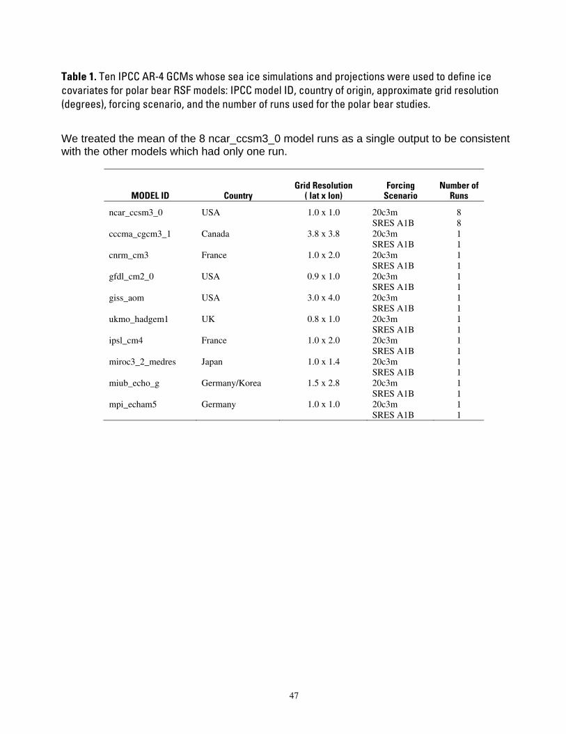
Table 1. Ten IPCC AR-4 GCMs whose sea ice simulations and projections were used to define ice covariates for polar bear RSF models: IPCC model ID, country of origin, approximate grid resolution (degrees), forcing scenario, and the number of runs used for the polar bear studies.

We treated the mean of the 8 ncar_ccsm3_0 model runs as a single output to be consistent with the other models which had only one run.

Grid Resolution Forcing Number of MODEL ID Country ( lat x lon) Scenario Runs

ncar_ccsm3_0

cccma_cgcm3_1

cnrm_cm3

gfdl_cm2_0

giss_aom

ukmo_hadgem1

ipsl_cm4

miroc3_2_medres

miub_echo_g

mpi_echam5

USA

Canada

France

USA

USA

UK

France

Japan

Germany/Korea

Germany

1.0 x 1.0

3.8 x 3.8

1.0 x 2.0

0.9 x 1.0

3.0 x 4.0

0.8 x 1.0

1.0 x 2.0

1.0 x 1.4

1.5 x 2.8

1.0 x 1.0

20c3m SRES A1B 20c3m SRES A1B 20c3m SRES A1B 20c3m SRES A1B 20c3m SRES A1B 20c3m SRES A1B 20c3m SRES A1B 20c3m SRES A1B 20c3m SRES A1B 20c3m SRES A1B

8 8 1 1 1 1 1 1 1 1 1 1 1 1 1 1 1 1 1 1

47

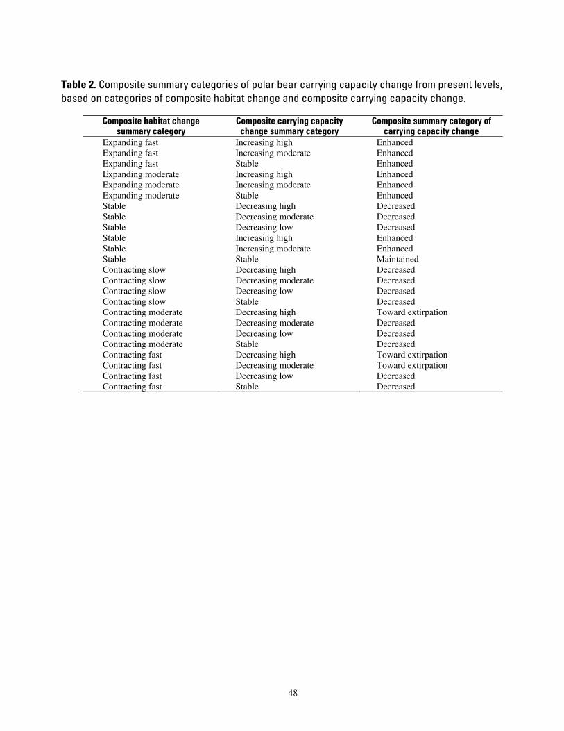
Table 2. Composite summary categories of polar bear carrying capacity change from present levels, based on categories of composite habitat change and composite carrying capacity change.

Composite habitat change Composite carrying capacity Composite summary category of summary category change summary category carrying capacity change

Expanding fast Increasing high Enhanced Expanding fast Increasing moderate Enhanced Expanding fast Stable Enhanced Expanding moderate Increasing high Enhanced Expanding moderate Increasing moderate Enhanced Expanding moderate Stable Enhanced Stable Decreasing high Decreased Stable Decreasing moderate Decreased Stable Decreasing low Decreased Stable Increasing high Enhanced Stable Increasing moderate Enhanced Stable Stable Maintained Contracting slow Decreasing high Decreased Contracting slow Decreasing moderate Decreased Contracting slow Decreasing low Decreased Contracting slow Stable Decreased Contracting moderate Decreasing high Toward extirpation Contracting moderate Decreasing moderate Decreased Contracting moderate Decreasing low Decreased Contracting moderate Stable Decreased Contracting fast Decreasing high Toward extirpation Contracting fast Decreasing moderate Toward extirpation Contracting fast Decreasing low Decreased Contracting fast Stable Decreased

48

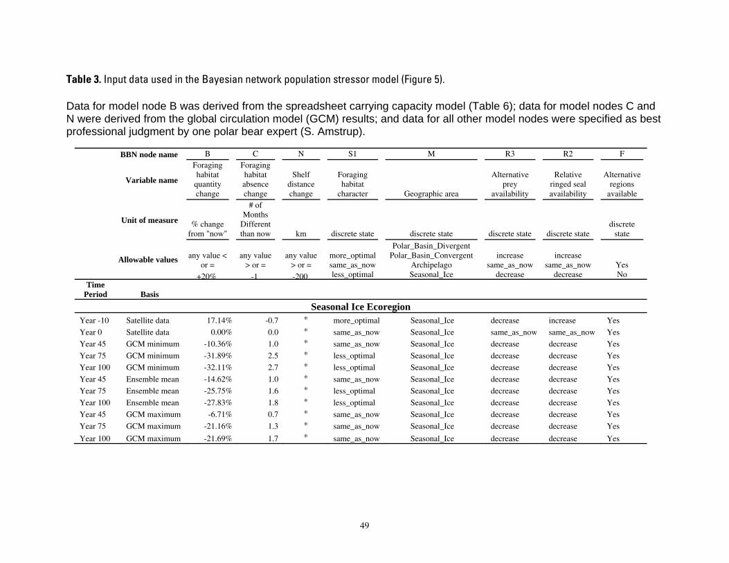
Table 3. Input data used in the Bayesian network population stressor model (Figure 5).

Data for model node B was derived from the spreadsheet carrying capacity model (Table 6); data for model nodes C and N were derived from the global circulation model (GCM) results; and data for all other model nodes were specified as best professional judgment by one polar bear expert (S. Amstrup).

BBN node name B C N S1 M R3 R2 F Foraging Foraging

Variable name habitat

quantity habitat absence

Shelf distance

Foraging habitat

Alternative prey

Relative ringed seal

Alternative regions

change change change character Geographic area availability availability available # of

Unit of measure % change Months

Different discrete from "now" than now km discrete state discrete state discrete state discrete state state

Polar_Basin_Divergent

Allowable values any value < or =

any value > or =

any value > or =

more_optimal same_as_now

Polar_Basin_Convergent Archipelago

increase same_as_now

increase same_as_now Yes

+20% -1 -200 less_optimal Seasonal_Ice decrease decrease No Time

Period Basis

Seasonal Ice Ecoregion Year -10 Satellite data 17.14% -0.7 * more_optimal Seasonal_Ice decrease increase Yes Year 0 Satellite data 0.00% 0.0 * same_as_now Seasonal_Ice same_as_now same_as_now Yes Year 45 GCM minimum -10.36% 1.0 * same_as_now Seasonal_Ice decrease decrease Yes Year 75 GCM minimum -31.89% 2.5 * less_optimal Seasonal_Ice decrease decrease Yes Year 100 GCM minimum -32.11% 2.7 * less_optimal Seasonal_Ice decrease decrease Yes Year 45 Ensemble mean -14.62% 1.0 * same_as_now Seasonal_Ice decrease decrease Yes Year 75 Ensemble mean -25.75% 1.6 * less_optimal Seasonal_Ice decrease decrease Yes Year 100 Ensemble mean -27.83% 1.8 * less_optimal Seasonal_Ice decrease decrease Yes Year 45 GCM maximum -6.71% 0.7 * same_as_now Seasonal_Ice decrease decrease Yes Year 75 GCM maximum -21.16% 1.3 * same_as_now Seasonal_Ice decrease decrease Yes

Year 100 GCM maximum -21.69% 1.7 * same_as_now Seasonal_Ice decrease decrease Yes

49

Table 3. continued.

BBN node name J1 B1 R1 J R4 T1 E T T2

Variable name Tourism

Bear-human interactions

Oil & gas activity Shipping

Hydrocarbons / oil spill Contaminants

Intentional takes

Parasites & disease Predation

Unit of measure discrete state discrete state discrete

state discrete state discrete state discrete state discrete state discrete

state discrete

state increased increased increase increased_occurrence elevated increased

Allowable values same_as_now same_as_now no_change increased same_as_now same_as_now same_as_now influential influential decreased decreased decrease same_as_now decreased_occurrence reduced decreased not not

Time period Basis

Seasonal Ice Ecoregion Year -10 Satellite data decreased decreased no_change same_as_now same_as_now reduced decreased not not

Year 0 Satellite data same_as_now same_as_now no_change same_as_now same_as_now same_as_now same_as_now not not

Year 45 GCM minimum increased increased no_change increased same_as_now elevated decreased influential influential

Year 75 GCM minimum increased increased no_change increased increased_occurrence elevated decreased influential influential

Year 100 GCM minimum increased increased no_change increased increased_occurrence elevated decreased influential influential

Year 45 Ensemble mean increased increased no_change increased same_as_now elevated decreased influential influential

Year 75 Ensemble mean increased increased no_change increased increased_occurrence elevated decreased influential influential

Year 100 Ensemble mean increased increased no_change increased increased_occurrence elevated decreased influential influential

Year 45 GCM maximum increased increased no_change increased same_as_now elevated decreased influential influential

Year 75 GCM maximum increased increased no_change increased increased_occurrence elevated decreased influential influential

Year 100 GCM maximum increased increased no_change increased increased_occurrence elevated decreased influential influential

50

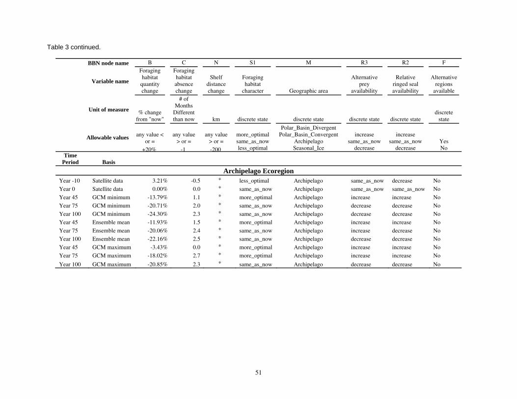
Table 3 continued.

BBN node name B C N S1 M R3 R2 F Foraging Foraging

Variable name habitat

quantity habitat absence

Shelf distance

Foraging habitat

Alternative prey

Relative ringed seal

Alternative regions

change change change character Geographic area availability availability available # of

Unit of measure % change Months

Different discrete from "now" than now km discrete state discrete state discrete state discrete state state

Polar_Basin_Divergent

Allowable values any value < or =

any value > or =

any value > or =

more_optimal same_as_now

Polar_Basin_Convergent Archipelago

increase same_as_now

increase same_as_now Yes

+20% -1 -200 less_optimal Seasonal_Ice decrease decrease No Time

Period Basis

Archipelago Ecoregion Year -10 Satellite data 3.21% -0.5 * less_optimal Archipelago same_as_now decrease No Year 0 Satellite data 0.00% 0.0 * same_as_now Archipelago same_as_now same_as_now No Year 45 GCM minimum -13.79% 1.1 * more_optimal Archipelago increase increase No Year 75 GCM minimum -20.71% 2.0 * same_as_now Archipelago decrease decrease No Year 100 GCM minimum -24.30% 2.3 * same_as_now Archipelago decrease decrease No Year 45 Ensemble mean -11.93% 1.5 * more_optimal Archipelago increase increase No Year 75 Ensemble mean -20.06% 2.4 * same_as_now Archipelago increase decrease No Year 100 Ensemble mean -22.16% 2.5 * same_as_now Archipelago decrease decrease No Year 45 GCM maximum -3.43% 0.0 * more_optimal Archipelago increase increase No Year 75 GCM maximum -18.02% 2.7 * more_optimal Archipelago increase increase No

Year 100 GCM maximum -20.85% 2.3 * same_as_now Archipelago decrease decrease No

51

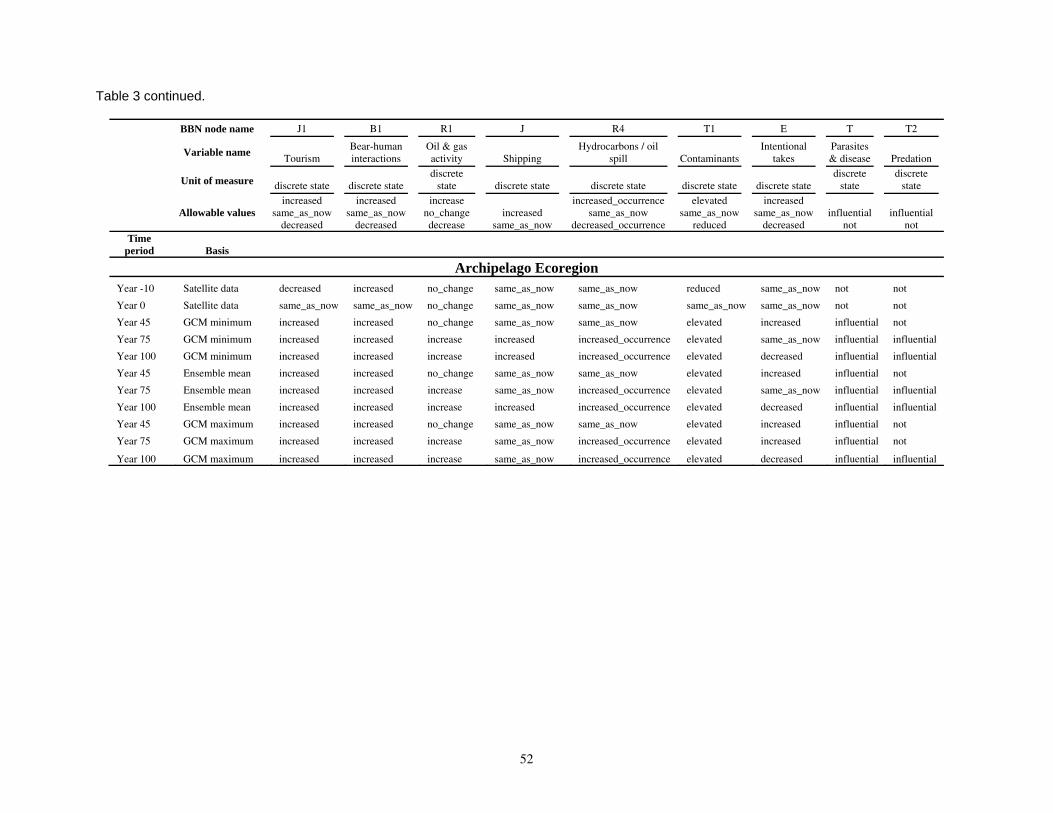
Table 3 continued.

BBN node name J1 B1 R1 J R4 T1 E T T2

Variable name Tourism

Bear-human interactions

Oil & gas activity Shipping

Hydrocarbons / oil spill Contaminants

Intentional takes

Parasites & disease Predation

Unit of measure discrete state discrete state discrete

state discrete state discrete state discrete state discrete state discrete

state discrete

state increased increased increase increased_occurrence elevated increased

Allowable values same_as_now same_as_now no_change increased same_as_now same_as_now same_as_now influential influential decreased decreased decrease same_as_now decreased_occurrence reduced decreased not not

Time period Basis

Archipelago Ecoregion Year -10 Satellite data decreased increased no_change same_as_now same_as_now reduced same_as_now not not

Year 0 Satellite data same_as_now same_as_now no_change same_as_now same_as_now same_as_now same_as_now not not

Year 45 GCM minimum increased increased no_change same_as_now same_as_now elevated increased influential not

Year 75 GCM minimum increased increased increase increased increased_occurrence elevated same_as_now influential influential

Year 100 GCM minimum increased increased increase increased increased_occurrence elevated decreased influential influential

Year 45 Ensemble mean increased increased no_change same_as_now same_as_now elevated increased influential not

Year 75 Ensemble mean increased increased increase same_as_now increased_occurrence elevated same_as_now influential influential

Year 100 Ensemble mean increased increased increase increased increased_occurrence elevated decreased influential influential

Year 45 GCM maximum increased increased no_change same_as_now same_as_now elevated increased influential not

Year 75 GCM maximum increased increased increase same_as_now increased_occurrence elevated increased influential not

Year 100 GCM maximum increased increased increase same_as_now increased_occurrence elevated decreased influential influential

52

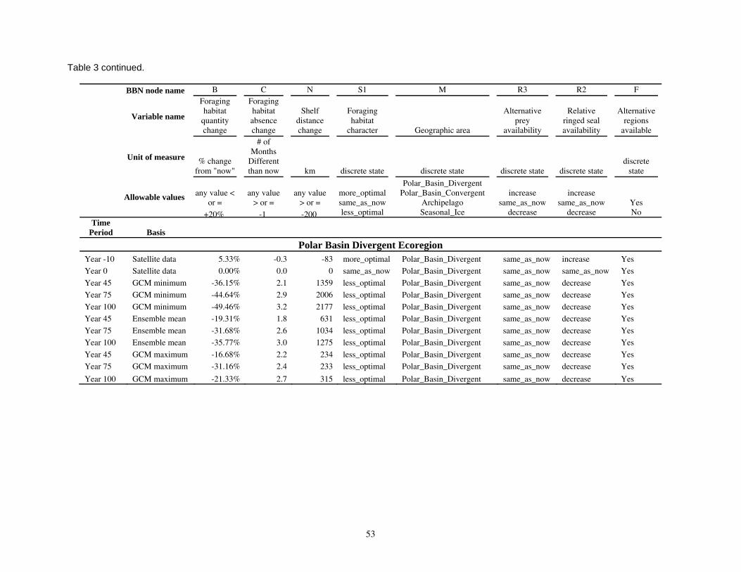
Table 3 continued.

BBN node name B C N S1 M R3 R2 F Foraging Foraging

Variable name habitat

quantity habitat absence

Shelf distance

Foraging habitat

Alternative prey

Relative ringed seal

Alternative regions

change change change character Geographic area availability availability available # of

Unit of measure % change Months

Different discrete from "now" than now km discrete state discrete state discrete state discrete state state

Polar_Basin_Divergent

Allowable values any value < or =

any value > or =

any value > or =

more_optimal same_as_now

Polar_Basin_Convergent Archipelago

increase same_as_now

increase same_as_now Yes

+20% -1 -200 less_optimal Seasonal_Ice decrease decrease No Time

Period Basis

Polar Basin Divergent Ecoregion Year -10 Satellite data 5.33% -0.3 -83 more_optimal Polar_Basin_Divergent same_as_now increase Yes Year 0 Satellite data 0.00% 0.0 0 same_as_now Polar_Basin_Divergent same_as_now same_as_now Yes Year 45 GCM minimum -36.15% 2.1 1359 less_optimal Polar_Basin_Divergent same_as_now decrease Yes Year 75 GCM minimum -44.64% 2.9 2006 less_optimal Polar_Basin_Divergent same_as_now decrease Yes Year 100 GCM minimum -49.46% 3.2 2177 less_optimal Polar_Basin_Divergent same_as_now decrease Yes Year 45 Ensemble mean -19.31% 1.8 631 less_optimal Polar_Basin_Divergent same_as_now decrease Yes Year 75 Ensemble mean -31.68% 2.6 1034 less_optimal Polar_Basin_Divergent same_as_now decrease Yes Year 100 Ensemble mean -35.77% 3.0 1275 less_optimal Polar_Basin_Divergent same_as_now decrease Yes Year 45 GCM maximum -16.68% 2.2 234 less_optimal Polar_Basin_Divergent same_as_now decrease Yes Year 75 GCM maximum -31.16% 2.4 233 less_optimal Polar_Basin_Divergent same_as_now decrease Yes

Year 100 GCM maximum -21.33% 2.7 315 less_optimal Polar_Basin_Divergent same_as_now decrease Yes

53

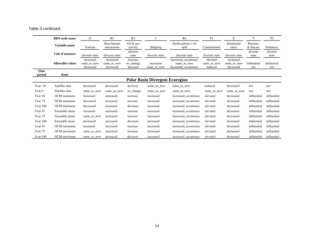
Table 3 continued.

BBN node name J1 B1 R1 J R4 T1 E T T2

Variable name Tourism

Bear-human interactions

Oil & gas activity Shipping

Hydrocarbons / oil spill Contaminants

Intentional takes

Parasites & disease Predation

Unit of measure discrete state discrete state discrete

state discrete state discrete state discrete state discrete state discrete

state discrete

state increased increased increase increased_occurrence elevated increased

Allowable values same_as_now same_as_now no_change increased same_as_now same_as_now same_as_now influential influential decreased decreased decrease same_as_now decreased_occurrence reduced decreased not not

Time period Basis

Polar Basin Divergent Ecoregion Year -10 Satellite data decreased decreased decrease same_as_now same_as_now reduced decreased not not

Year 0 Satellite data same_as_now same_as_now no_change same_as_now same_as_now same_as_now same_as_now not not

Year 45 GCM minimum increased increased increase increased increased_occurrence elevated decreased influential influential

Year 75 GCM minimum decreased increased increase increased increased_occurrence elevated decreased influential influential

Year 100 GCM minimum decreased increased decrease increased increased_occurrence elevated decreased influential influential

Year 45 Ensemble mean increased increased increase increased increased_occurrence elevated decreased influential influential

Year 75 Ensemble mean same_as_now increased increase increased increased_occurrence elevated decreased influential influential

Year 100 Ensemble mean decreased increased decrease increased increased_occurrence elevated decreased influential influential

Year 45 GCM maximum increased increased increase increased increased_occurrence elevated decreased influential influential

Year 75 GCM maximum same_as_now increased increase increased increased_occurrence elevated decreased influential influential

Year 100 GCM maximum same_as_now increased decrease increased increased_occurrence elevated decreased influential influential

54

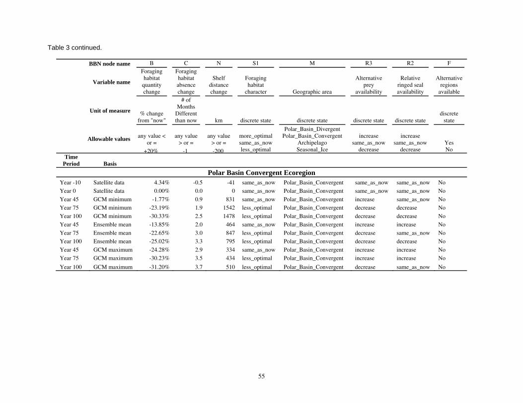
Table 3 continued.

BBN node name B C N S1 M R3 R2 F Foraging Foraging

Variable name habitat

quantity habitat absence

Shelf distance

Foraging habitat

Alternative prey

Relative ringed seal

Alternative regions

change change change character Geographic area availability availability available # of

Unit of measure % change Months

Different discrete from "now" than now km discrete state discrete state discrete state discrete state state

Polar_Basin_Divergent

Allowable values any value < or =

any value > or =

any value > or =

more_optimal same_as_now

Polar_Basin_Convergent Archipelago

increase same_as_now

increase same_as_now Yes

+20% -1 -200 less_optimal Seasonal_Ice decrease decrease No Time

Period Basis

Polar Basin Convergent Ecoregion Year -10 Satellite data 4.34% -0.5 -41 same_as_now Polar_Basin_Convergent same_as_now same_as_now No Year 0 Satellite data 0.00% 0.0 0 same_as_now Polar_Basin_Convergent same_as_now same_as_now No Year 45 GCM minimum -1.77% 0.9 831 same_as_now Polar_Basin_Convergent increase same_as_now No Year 75 GCM minimum -23.19% 1.9 1542 less_optimal Polar_Basin_Convergent decrease decrease No Year 100 GCM minimum -30.33% 2.5 1478 less_optimal Polar_Basin_Convergent decrease decrease No Year 45 Ensemble mean -13.85% 2.0 464 same_as_now Polar_Basin_Convergent increase increase No Year 75 Ensemble mean -22.65% 3.0 847 less_optimal Polar_Basin_Convergent decrease same_as_now No Year 100 Ensemble mean -25.02% 3.3 795 less_optimal Polar_Basin_Convergent decrease decrease No Year 45 GCM maximum -24.28% 2.9 334 same_as_now Polar_Basin_Convergent increase increase No Year 75 GCM maximum -30.23% 3.5 434 less_optimal Polar_Basin_Convergent increase increase No

Year 100 GCM maximum -31.20% 3.7 510 less_optimal Polar_Basin_Convergent decrease same_as_now No

55

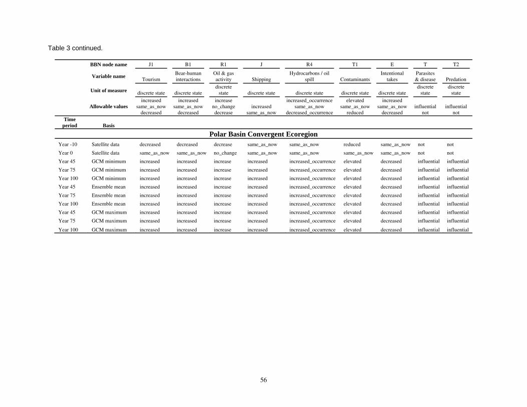
Table 3 continued.

BBN node name J1 B1 R1 J R4 T1 E T T2

Variable name Tourism

Bear-human interactions

Oil & gas activity Shipping

Hydrocarbons / oil spill Contaminants

Intentional takes

Parasites & disease Predation

Unit of measure discrete state discrete state discrete

state discrete state discrete state discrete state discrete state discrete

state discrete

state increased increased increase increased_occurrence elevated increased

Allowable values same_as_now same_as_now no_change increased same_as_now same_as_now same_as_now influential influential decreased decreased decrease same_as_now decreased_occurrence reduced decreased not not

Time period Basis

Polar Basin Convergent Ecoregion Year -10 Satellite data decreased decreased decrease same_as_now same_as_now reduced same_as_now not not

Year 0 Satellite data same_as_now same_as_now no_change same_as_now same_as_now same_as_now same_as_now not not

Year 45 GCM minimum increased increased increase increased increased_occurrence elevated decreased influential influential

Year 75 GCM minimum increased increased increase increased increased_occurrence elevated decreased influential influential

Year 100 GCM minimum increased increased increase increased increased_occurrence elevated decreased influential influential

Year 45 Ensemble mean increased increased increase increased increased_occurrence elevated decreased influential influential

Year 75 Ensemble mean increased increased increase increased increased_occurrence elevated decreased influential influential

Year 100 Ensemble mean increased increased increase increased increased_occurrence elevated decreased influential influential

Year 45 GCM maximum increased increased increase increased increased_occurrence elevated decreased influential influential

Year 75 GCM maximum increased increased increase increased increased_occurrence elevated decreased influential influential

Year 100 GCM maximum increased increased increase increased increased_occurrence elevated decreased influential influential

56

Table 4. Amount, percent change, and summary of change in polar bear habitat forecasted by the deterministic polar bear carrying capacity model.

x = not calculated or data not available.

Habitat amount (km2-months x 1000)

% change in habitat from year 0 Change in Total Habitat from Year 0

Time Period

Year -10

Year 0

Year 0

Year 45

Year 75

Year 100

Year 0

Year 45

Year 75

Year 100

Year 0

Year 45

Year 75

Year 100

Data basis

Satellite data

Satellite data

GCM minimum

GCM minimum

GCM minimum

GCM minimum

Ensemble mean

Ensemble mean

Ensemble mean

Ensemble mean

GCM maximum

GCM maximum

GCM maximum

GCM maximum

Total habitat RSF habitat Non-RSF habitat RSF habitat Total habitat

Seasonal Ice Ecoregion 16,258.70 x x x 17%

13,879.60 x x x 0%

11,217.33 x x x 0%

10,054.93 x x x -10%

7,640.68 x x x -32%

7,615.55 x x x -32%

16,340.56 x x x 0%

13,952.36 x x x -15%

12,132.32 x x x -26%

11,793.25 x x x -28%

20,178.76 x x x 0%

18,823.83 x x x -7%

15,909.29 x x x -21%

15,802.26 x x x -22%

Direction1 Magnitude2 Summary

Expanding or stable Moderate Expanding moderate

Expanding or stable Slow to none Stable

Expanding or stable Slow to none Stable

Contracting Slow to none Contracting slow

Contracting Fast Contracting fast

Contracting Fast Contracting fast

Expanding or stable Slow to none Stable

Contracting Slow to none Contracting slow

Contracting Moderate Contracting moderate

Contracting Moderate Contracting moderate

Expanding or stable Slow to none Stable

Contracting Slow to none Contracting slow

Contracting Moderate Contracting moderate

Contracting Moderate Contracting moderate

1 Direction was categorized into “contracting” if CHt G < 0 or “expanding or stable” if CHt G ≥ 0 . , ,

2 Magnitude was categorized into “fast” if CH > 30.0 , “moderate” if 15.0 < CH ≤ 30.0 , and “slow or none” if CH <15.0.t ,G t ,G t ,G

57

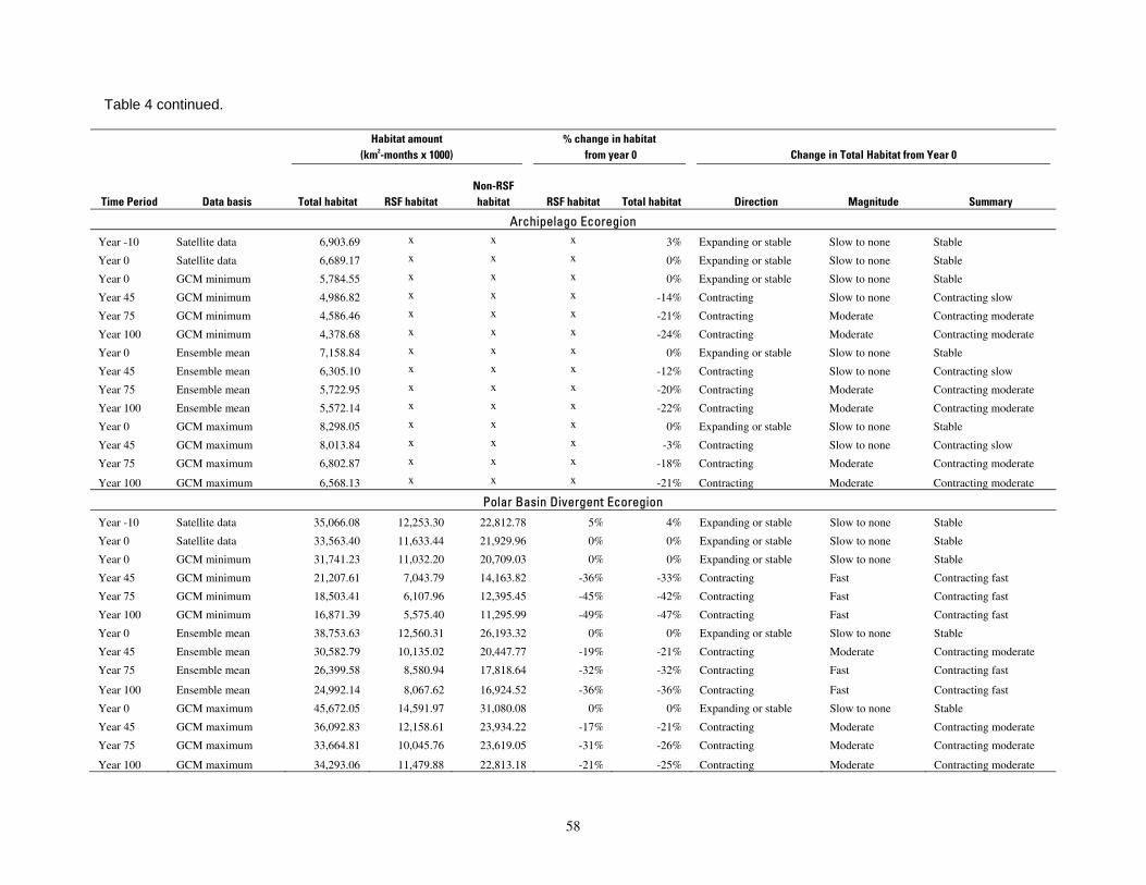
Table 4 continued.

Habitat amount (km2-months x 1000)

% change in habitat from year 0 Change in Total Habitat from Year 0

Time Period Data basis Total habitat RSF habitat Non-RSF habitat RSF habitat Total habitat Direction Magnitude Summary

Archipelago Ecoregion Year -10 Satellite data 6,903.69 x x x 3% Expanding or stable Slow to none Stable

Year 0 Satellite data 6,689.17 x x x 0% Expanding or stable Slow to none Stable

Year 0 GCM minimum 5,784.55 x x x 0% Expanding or stable Slow to none Stable

Year 45 GCM minimum 4,986.82 x x x -14% Contracting Slow to none Contracting slow

Year 75 GCM minimum 4,586.46 x x x -21% Contracting Moderate Contracting moderate

Year 100 GCM minimum 4,378.68 x x x -24% Contracting Moderate Contracting moderate

Year 0 Ensemble mean 7,158.84 x x x 0% Expanding or stable Slow to none Stable

Year 45 Ensemble mean 6,305.10 x x x -12% Contracting Slow to none Contracting slow

Year 75 Ensemble mean 5,722.95 x x x -20% Contracting Moderate Contracting moderate

Year 100 Ensemble mean 5,572.14 x x x -22% Contracting Moderate Contracting moderate

Year 0 GCM maximum 8,298.05 x x x 0% Expanding or stable Slow to none Stable

Year 45 GCM maximum 8,013.84 x x x -3% Contracting Slow to none Contracting slow

Year 75 GCM maximum 6,802.87 x x x -18% Contracting Moderate Contracting moderate

Year 100 GCM maximum 6,568.13 x x x -21% Contracting Moderate Contracting moderate

Polar Basin Divergent Ecoregion Year -10 Satellite data 35,066.08 12,253.30 22,812.78 5% 4% Expanding or stable Slow to none Stable

Year 0 Satellite data 33,563.40 11,633.44 21,929.96 0% 0% Expanding or stable Slow to none Stable

Year 0 GCM minimum 31,741.23 11,032.20 20,709.03 0% 0% Expanding or stable Slow to none Stable

Year 45 GCM minimum 21,207.61 7,043.79 14,163.82 -36% -33% Contracting Fast Contracting fast

Year 75 GCM minimum 18,503.41 6,107.96 12,395.45 -45% -42% Contracting Fast Contracting fast

Year 100 GCM minimum 16,871.39 5,575.40 11,295.99 -49% -47% Contracting Fast Contracting fast

Year 0 Ensemble mean 38,753.63 12,560.31 26,193.32 0% 0% Expanding or stable Slow to none Stable

Year 45 Ensemble mean 30,582.79 10,135.02 20,447.77 -19% -21% Contracting Moderate Contracting moderate

Year 75 Ensemble mean 26,399.58 8,580.94 17,818.64 -32% -32% Contracting Fast Contracting fast

Year 100 Ensemble mean 24,992.14 8,067.62 16,924.52 -36% -36% Contracting Fast Contracting fast

Year 0 GCM maximum 45,672.05 14,591.97 31,080.08 0% 0% Expanding or stable Slow to none Stable

Year 45 GCM maximum 36,092.83 12,158.61 23,934.22 -17% -21% Contracting Moderate Contracting moderate

Year 75 GCM maximum 33,664.81 10,045.76 23,619.05 -31% -26% Contracting Moderate Contracting moderate

Year 100 GCM maximum 34,293.06 11,479.88 22,813.18 -21% -25% Contracting Moderate Contracting moderate

58

Table 4 continued.

Habitat amount (km2-months x 1000)

% change in habitat from year 0 Change in Total Habitat from Year 0

Time Period Data basis Total habitat RSF habitat Non-RSF habitat RSF habitat Total habitat Direction Magnitude Summary

Polar Basin Convergent Ecoregion Year -10 Satellite data 6,063.56 5,440.34 623.22 4% 4% Expanding or stable Slow to none Stable

Year 0 Satellite data 5,823.36 5,214.13 609.23 0% 0% Expanding or stable Slow to none Stable

Year 0 GCM minimum 4,945.44 4,136.50 808.94 0% 0% Expanding or stable Slow to none Stable

Year 45 GCM minimum 4,424.39 4,063.23 361.16 -2% -11% Contracting Slow to none Contracting slow

Year 75 GCM minimum 4,042.15 3,177.04 865.11 -23% -18% Contracting Moderate Contracting moderate

Year 100 GCM minimum 3,539.31 2,881.99 657.32 -30% -28% Contracting Moderate Contracting moderate

Year 0 Ensemble mean 6,305.23 5,158.01 1,147.22 0% 0% Expanding or stable Slow to none Stable

Year 45 Ensemble mean 5,334.67 4,443.39 891.28 -14% -15% Contracting Moderate Contracting moderate

Year 75 Ensemble mean 4,739.31 3,989.57 749.74 -23% -25% Contracting Moderate Contracting moderate

Year 100 Ensemble mean 4,566.56 3,867.34 699.22 -25% -28% Contracting Moderate Contracting moderate

Year 0 GCM maximum 7,068.41 6,023.03 1,045.38 0% 0% Expanding or stable Slow to none Stable

Year 45 GCM maximum 6,115.28 4,560.71 1,554.57 -24% -13% Contracting Slow to none Contracting slow

Year 75 GCM maximum 5,538.43 4,202.23 1,336.20 -30% -22% Contracting Moderate Contracting moderate

Year 100 GCM maximum 5,625.88 4,143.95 1,481.93 -31% -20% Contracting Moderate Contracting moderate

Global (all ecoregions combined) Year -10 Satellite data 64,292.03 x x x 7% Expanding or stable Slow to none Stable

Year 0 Satellite data 59,955.53 x x x 0% Expanding or stable Slow to none Stable

Year 0 GCM minimum 53,688.55 x x x 0% Expanding or stable Slow to none Stable

Year 45 GCM minimum 40,673.75 x x x -24% Contracting Moderate Contracting moderate

Year 75 GCM minimum 34,772.70 x x x -35% Contracting Fast Contracting fast

Year 100 GCM minimum 32,404.93 x x x -40% Contracting Fast Contracting fast

Year 0 Ensemble mean 68,558.26 x x x 0% Expanding or stable Slow to none Stable

Year 45 Ensemble mean 56,174.92 x x x -18% Contracting Moderate Contracting moderate

Year 75 Ensemble mean 48,994.16 x x x -29% Contracting Moderate Contracting moderate

Year 100 Ensemble mean 46,924.09 x x x -32% Contracting Fast Contracting fast

Year 0 GCM maximum 81,217.27 x x x 0% Expanding or stable Slow to none Stable

Year 45 GCM maximum 69,045.78 x x x -15% Contracting Slow to none Contracting slow

Year 75 GCM maximum 61,915.40 x x x -24% Contracting Moderate Contracting moderate

Year 100 GCM maximum 62,289.33 x x x -23% Contracting Moderate Contracting moderate

59

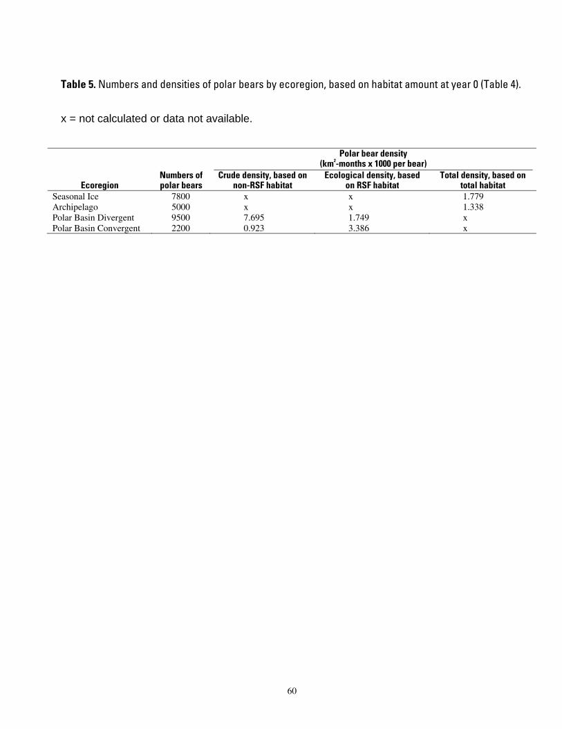
Table 5. Numbers and densities of polar bears by ecoregion, based on habitat amount at year 0 (Table 4).

x = not calculated or data not available.

Polar bear density (km2-months x 1000 per bear)

Numbers of Crude density, based on Ecological density, based Total density, based on Ecoregion polar bears non-RSF habitat on RSF habitat total habitat

Seasonal Ice 7800 x x 1.779 Archipelago 5000 x x 1.338 Polar Basin Divergent 9500 7.695 1.749 x Polar Basin Convergent 2200 0.923 3.386 x

60

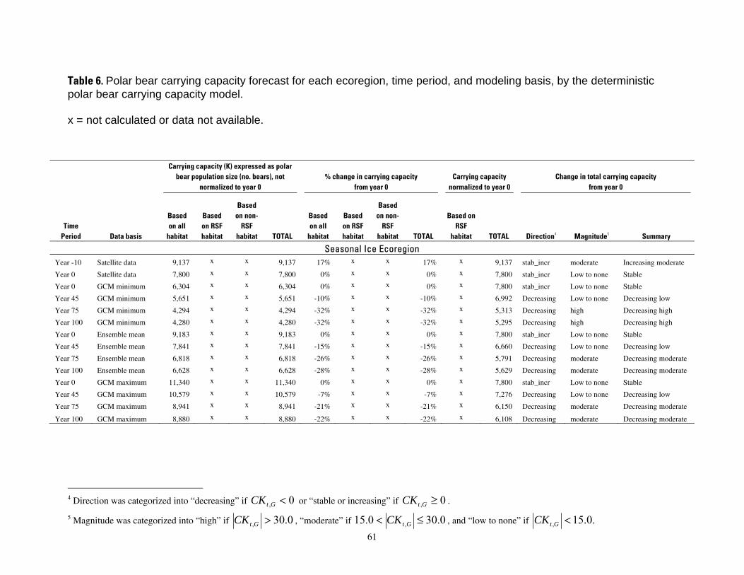
Table 6. Polar bear carrying capacity forecast for each ecoregion, time period, and modeling basis, by the deterministic polar bear carrying capacity model.

x = not calculated or data not available.

Carrying capacity (K) expressed as polar bear population size (no. bears), not

normalized to year 0 % change in carrying capacity

from year 0 Carrying capacity

normalized to year 0 Change in total carrying capacity

from year 0

Time Period Data basis

Based on all

habitat

Based on RSF habitat

Based on non-

RSF habitat TOTAL

Based on all

habitat

Based on RSF habitat

Based on non-

RSF habitat TOTAL

Based on RSF

habitat TOTAL Direction4 Magnitude5 Summary

Seasonal Ice Ecoregion Year -10 Satellite data 9,137 x x 9,137 17% x x 17% x 9,137 stab_incr moderate Increasing moderate

Year 0 Satellite data 7,800 x x 7,800 0% x x 0% x 7,800 stab_incr Low to none Stable

Year 0 GCM minimum 6,304 x x 6,304 0% x x 0% x 7,800 stab_incr Low to none Stable

Year 45 GCM minimum 5,651 x x 5,651 -10% x x -10% x 6,992 Decreasing Low to none Decreasing low

Year 75 GCM minimum 4,294 x x 4,294 -32% x x -32% x 5,313 Decreasing high Decreasing high

Year 100 GCM minimum 4,280 x x 4,280 -32% x x -32% x 5,295 Decreasing high Decreasing high

Year 0 Ensemble mean 9,183 x x 9,183 0% x x 0% x 7,800 stab_incr Low to none Stable

Year 45 Ensemble mean 7,841 x x 7,841 -15% x x -15% x 6,660 Decreasing Low to none Decreasing low

Year 75 Ensemble mean 6,818 x x 6,818 -26% x x -26% x 5,791 Decreasing moderate Decreasing moderate

Year 100 Ensemble mean 6,628 x x 6,628 -28% x x -28% x 5,629 Decreasing moderate Decreasing moderate

Year 0 GCM maximum 11,340 x x 11,340 0% x x 0% x 7,800 stab_incr Low to none Stable

Year 45 GCM maximum 10,579 x x 10,579 -7% x x -7% x 7,276 Decreasing Low to none Decreasing low

Year 75 GCM maximum 8,941 x x 8,941 -21% x x -21% x 6,150 Decreasing moderate Decreasing moderate

Year 100 GCM maximum 8,880 x x 8,880 -22% x x -22% x 6,108 Decreasing moderate Decreasing moderate

4 Direction was categorized into “decreasing” if CKt ,G < 0 or “stable or increasing” if CKt ,G ≥ 0 . 5 Magnitude was categorized into “high” if CK > 30.0 , “moderate” if 15.0 < CK ≤ 30.0 , and “low to none” if t ,G t ,G

61

CK < 15.0.t ,G

Table 6 continued. Carrying capacity (K) expressed as polar

bear population size (no. bears), not % change in carrying capacity Carrying capacity Change in total carrying capacity normalized to year 0 from year 0 normalized to year 0 from year 0

Based Based Based Based on non- Based Based on non- Based on

Time on all on RSF RSF on all on RSF RSF RSF Period Data basis habitat habitat habitat TOTAL habitat habitat habitat TOTAL habitat TOTAL Direction Magnitude Summary

Archipelago Ecoregion Year -10 Satellite data 5,160 x x 5,160 3% x x 3% x 5,160 stab_incr Low to none Stable

Year 0 Satellite data 5,000 x x 5,000 0% x x 0% x 5,000 stab_incr Low to none Stable

Year 0 GCM minimum 4,324 x x 4,324 0% x x 0% x 5,000 stab_incr Low to none Stable

Year 45 GCM minimum 3,728 x x 3,728 -14% x x -14% x 4,310 Decreasing Low to none Decreasing low

Year 75 GCM minimum 3,428 x x 3,428 -21% x x -21% x 3,964 Decreasing Moderate Decreasing moderate

Year 100 GCM minimum 3,273 x x 3,273 -24% x x -24% x 3,785 Decreasing Moderate Decreasing moderate

Year 0 Ensemble mean 5,351 x x 5,351 0% x x 0% x 5,000 Stable-Incr Low to none Stable

Year 45 Ensemble mean 4,713 x x 4,713 -12% x x -12% x 4,404 Decreasing Low to none Decreasing low

Year 75 Ensemble mean 4,278 x x 4,278 -20% x x -20% x 3,997 Decreasing Moderate Decreasing moderate

Year 100 Ensemble mean 4,165 x x 4,165 -22% x x -22% x 3,892 Decreasing Moderate Decreasing moderate

Year 0 GCM maximum 6,203 x x 6,203 0% x x 0% x 5,000 Stable-Incr Low to none Stable

Year 45 GCM maximum 5,990 x x 5,990 -3% x x -3% x 4,829 Decreasing Low to none Decreasing low

Year 75 GCM maximum 5,085 x x 5,085 -18% x x -18% x 4,099 Decreasing Moderate Decreasing moderate

Year 100 GCM maximum 4,910 x x 4,910 -21% x x -21% x 3,958 Decreasing Moderate Decreasing moderate

Polar Basin Divergent Ecoregion Year -10 Satellite data x 7,004 2,965 9,969 x 5% 4% 5% 7,004 9,969 Stable-Incr Low to none Stable

Year 0 Satellite data x 6,650 2,850 9,500 x 0% 0% 0% 6,650 9,500 Stable-Incr Low to none Stable

Year 0 GCM minimum x 6,306 2,691 8,998 x 0% 0% 0% 6,650 9,500 Stable-Incr Low to none Stable

Year 45 GCM minimum x 4,026 1,841 5,867 x -36% -32% -35% 4,246 6,195 Decreasing High Decreasing high

Year 75 GCM minimum x 3,491 1,611 5,102 x -45% -40% -43% 3,682 5,387 Decreasing High Decreasing high

Year 100 GCM minimum x 3,187 1,468 4,655 x -49% -45% -48% 3,361 4,915 Decreasing High Decreasing high

Year 0 Ensemble mean x 7,180 3,404 10,584 x 0% 0% 0% 6,650 9,500 Stable-Incr Low to none Stable

Year 45 Ensemble mean x 5,793 2,657 8,451 x -19% -22% -20% 5,366 7,585 Decreasing Moderate Decreasing moderate

Year 75 Ensemble mean x 4,905 2,316 7,221 x -32% -32% -32% 4,543 6,481 Decreasing High Decreasing high

Year 100 Ensemble mean x 4,612 2,199 6,811 x -36% -35% -36% 4,271 6,114 Decreasing High Decreasing high

Year 0 GCM maximum x 8,341 4,039 12,380 x 0% 0% 0% 6,650 9,500 Stable-Incr Low to none Stable

Year 45 GCM maximum x 6,950 3,110 10,061 x -17% -23% -19% 5,541 7,720 Decreasing Moderate Decreasing moderate

Year 75 GCM maximum x 5,742 3,070 8,812 x -31% -24% -29% 4,578 6,762 Decreasing Moderate Decreasing moderate

Year 100 GCM maximum x 6,562 2,965 9,527 x -21% -27% -23% 5,232 7,311 Decreasing Moderate Decreasing moderate

62

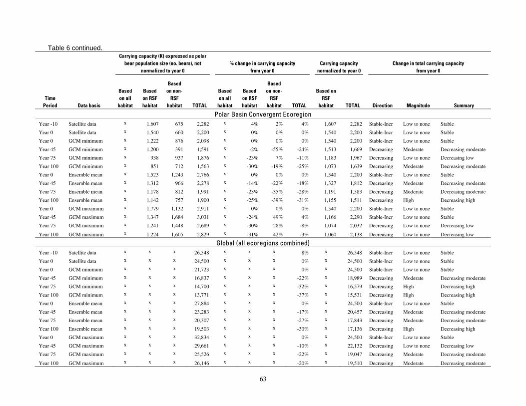
Table 6 continued. Carrying capacity (K) expressed as polar

bear population size (no. bears), not % change in carrying capacity Carrying capacity Change in total carrying capacity normalized to year 0 from year 0 normalized to year 0 from year 0

Based Based Based Based on non- Based Based on non- Based on

Time on all on RSF RSF on all on RSF RSF RSF Period Data basis habitat habitat habitat TOTAL habitat habitat habitat TOTAL habitat TOTAL Direction Magnitude Summary

Polar Basin Convergent Ecoregion Year -10 Satellite data x 1,607 675 2,282 x 4% 2% 4% 1,607 2,282 Stable-Incr Low to none Stable

Year 0 Satellite data x 1,540 660 2,200 x 0% 0% 0% 1,540 2,200 Stable-Incr Low to none Stable

Year 0 GCM minimum x 1,222 876 2,098 x 0% 0% 0% 1,540 2,200 Stable-Incr Low to none Stable

Year 45 GCM minimum x 1,200 391 1,591 x -2% -55% -24% 1,513 1,669 Decreasing Moderate Decreasing moderate

Year 75 GCM minimum x 938 937 1,876 x -23% 7% -11% 1,183 1,967 Decreasing Low to none Decreasing low

Year 100 GCM minimum x 851 712 1,563 x -30% -19% -25% 1,073 1,639 Decreasing Moderate Decreasing moderate

Year 0 Ensemble mean x 1,523 1,243 2,766 x 0% 0% 0% 1,540 2,200 Stable-Incr Low to none Stable

Year 45 Ensemble mean x 1,312 966 2,278 x -14% -22% -18% 1,327 1,812 Decreasing Moderate Decreasing moderate

Year 75 Ensemble mean x 1,178 812 1,991 x -23% -35% -28% 1,191 1,583 Decreasing Moderate Decreasing moderate

Year 100 Ensemble mean x 1,142 757 1,900 x -25% -39% -31% 1,155 1,511 Decreasing High Decreasing high

Year 0 GCM maximum x 1,779 1,132 2,911 x 0% 0% 0% 1,540 2,200 Stable-Incr Low to none Stable

Year 45 GCM maximum x 1,347 1,684 3,031 x -24% 49% 4% 1,166 2,290 Stable-Incr Low to none Stable

Year 75 GCM maximum x 1,241 1,448 2,689 x -30% 28% -8% 1,074 2,032 Decreasing Low to none Decreasing low

Year 100 GCM maximum x 1,224 1,605 2,829 x -31% 42% -3% 1,060 2,138 Decreasing Low to none Decreasing low

Global (all ecoregions combined) Year -10 Satellite data x x x 26,548 x x x 8% x 26,548 Stable-Incr Low to none Stable

Year 0 Satellite data x x x 24,500 x x x 0% x 24,500 Stable-Incr Low to none Stable

Year 0 GCM minimum x x x 21,723 x x x 0% x 24,500 Stable-Incr Low to none Stable

Year 45 GCM minimum x x x 16,837 x x x -22% x 18,989 Decreasing Moderate Decreasing moderate

Year 75 GCM minimum x x x 14,700 x x x -32% x 16,579 Decreasing High Decreasing high

Year 100 GCM minimum x x x 13,771 x x x -37% x 15,531 Decreasing High Decreasing high

Year 0 Ensemble mean x x x 27,884 x x x 0% x 24,500 Stable-Incr Low to none Stable

Year 45 Ensemble mean x x x 23,283 x x x -17% x 20,457 Decreasing Moderate Decreasing moderate

Year 75 Ensemble mean x x x 20,307 x x x -27% x 17,843 Decreasing Moderate Decreasing moderate

Year 100 Ensemble mean x x x 19,503 x x x -30% x 17,136 Decreasing High Decreasing high

Year 0 GCM maximum x x x 32,834 x x x 0% x 24,500 Stable-Incr Low to none Stable

Year 45 GCM maximum x x x 29,661 x x x -10% x 22,132 Decreasing Low to none Decreasing low

Year 75 GCM maximum x x x 25,526 x x x -22% x 19,047 Decreasing Moderate Decreasing moderate

Year 100 GCM maximum x x x 26,146 x x x -20% x 19,510 Decreasing Moderate Decreasing moderate

63

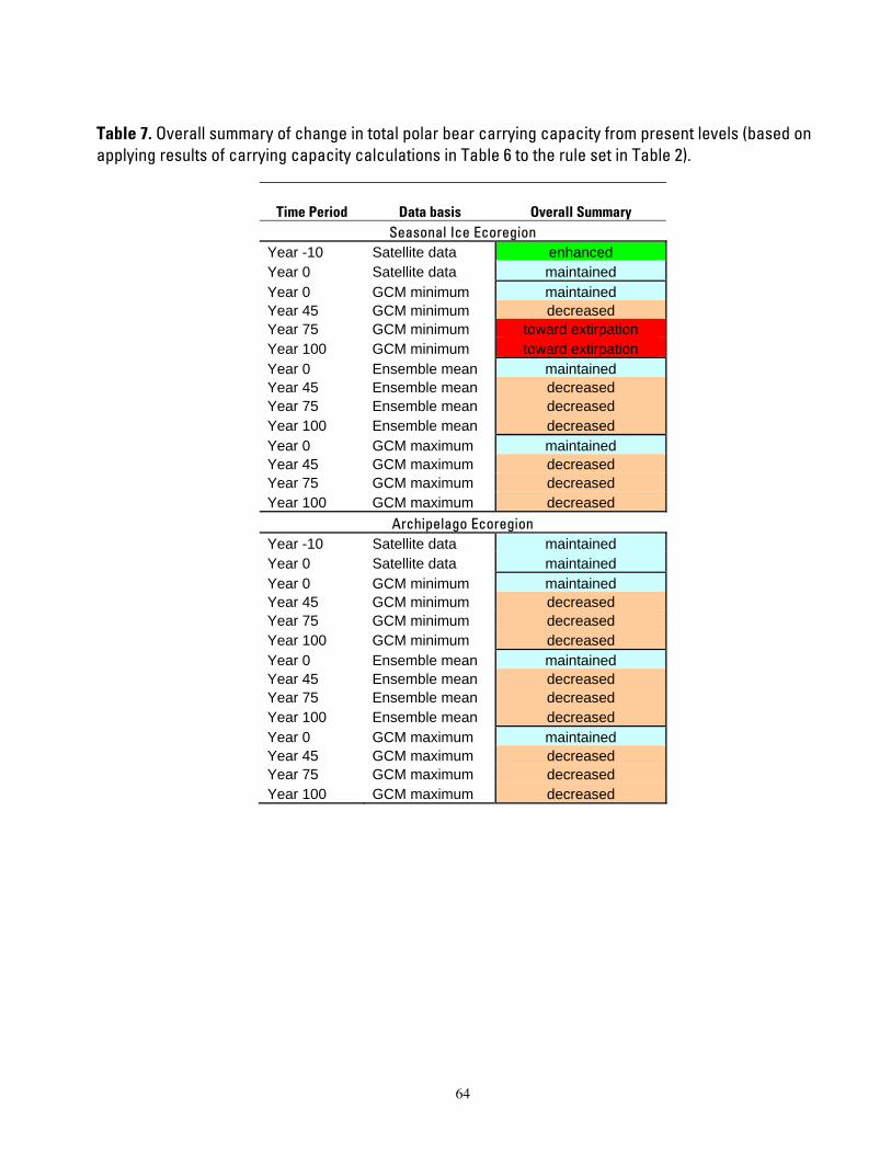
Table 7. Overall summary of change in total polar bear carrying capacity from present levels (based on applying results of carrying capacity calculations in Table 6 to the rule set in Table 2).

Time Period Data basis Overall Summary

Year -10 Satellite data Year 0 Satellite data Year 0 GCM minimum Year 45 GCM minimum Year 75 GCM minimum Year 100 GCM minimum

Seasonal Ice Ecoregion enhanced maintained maintained decreased

toward extirpation toward extirpation

maintained decreased decreased decreased maintained decreased decreased decreased

Year 0 Ensemble mean Year 45 Ensemble mean Year 75 Ensemble mean Year 100 Ensemble mean Year 0 GCM maximum Year 45 GCM maximum Year 75 GCM maximum Year 100 GCM maximum

Archipelago Ecoregion maintained maintained maintained decreased decreased decreased

Year -10 Satellite data Year 0 Satellite data Year 0 GCM minimum Year 45 GCM minimum Year 75 GCM minimum Year 100 GCM minimum Year 0 Ensemble mean Year 45 Ensemble mean Year 75 Ensemble mean Year 100 Ensemble mean Year 0 GCM maximum Year 45 GCM maximum Year 75 GCM maximum Year 100 GCM maximum

maintained decreased decreased decreased maintained decreased decreased decreased

64

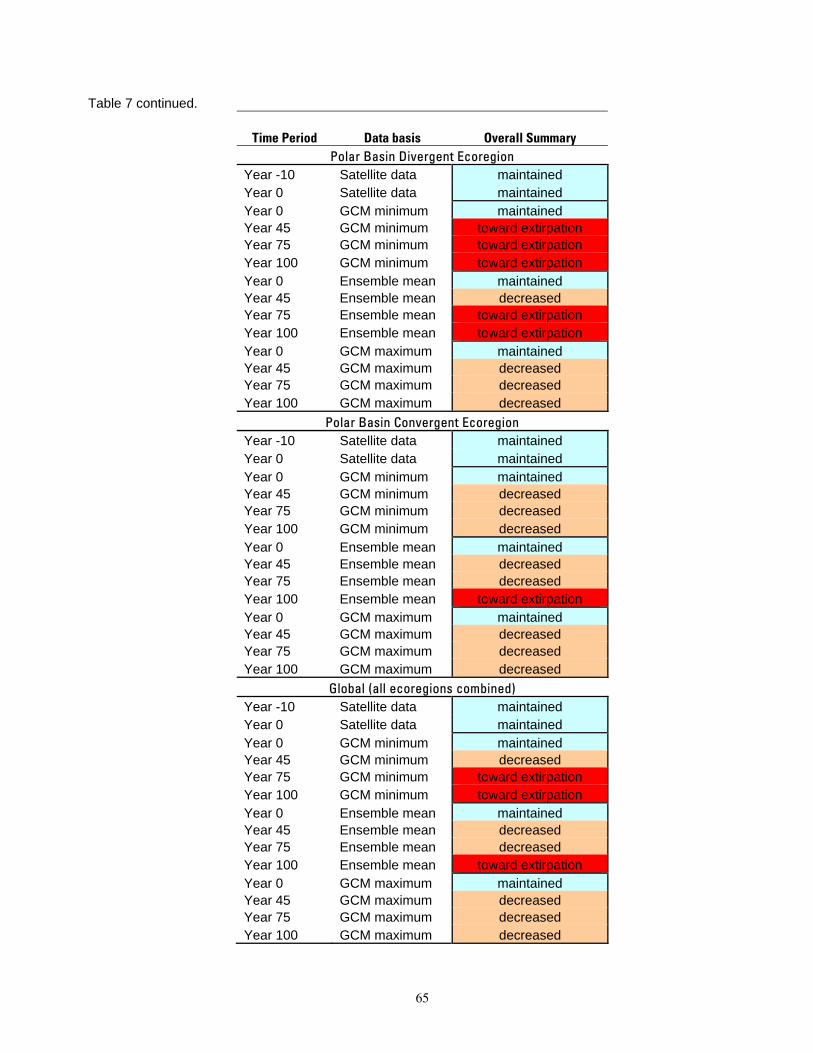
Table 7 continued.

Time Period Data basis Overall Summary

maintained maintained maintained

toward extirpation toward extirpation toward extirpation

Polar Basin Divergent Ecoregion Year -10 Satellite data Year 0 Satellite data Year 0 GCM minimum Year 45 GCM minimum Year 75 GCM minimum Year 100 GCM minimum Year 0 Ensemble mean Year 45 Ensemble mean Year 75 Ensemble mean Year 100 Ensemble mean Year 0 GCM maximum Year 45 GCM maximum Year 75 GCM maximum Year 100 GCM maximum

maintained decreased

toward extirpation toward extirpation

maintained decreased decreased decreased

Polar Basin Convergent Ecoregion Year -10 Satellite data maintained Year 0 Satellite data maintained Year 0 GCM minimum maintained Year 45 GCM minimum decreased Year 75 GCM minimum decreased Year 100 GCM minimum decreased Year 0 Ensemble mean maintained Year 45 Ensemble mean decreased Year 75 Ensemble mean decreased Year 100 Ensemble mean toward extirpation Year 0 GCM maximum maintained Year 45 GCM maximum decreased Year 75 GCM maximum decreased Year 100 GCM maximum decreased

Global (all ecoregions combined) Year -10 Satellite data maintained Year 0 Satellite data maintained Year 0 GCM minimum maintained Year 45 GCM minimum decreased Year 75 GCM minimum toward extirpation Year 100 GCM minimum toward extirpation Year 0 Ensemble mean maintained Year 45 Ensemble mean decreased Year 75 Ensemble mean decreased Year 100 Ensemble mean toward extirpation Year 0 GCM maximum maintained Year 45 GCM maximum decreased Year 75 GCM maximum decreased Year 100 GCM maximum decreased

65

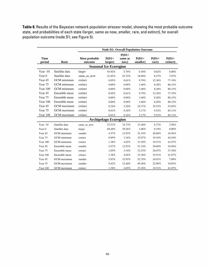
Table 8. Results of the Bayesian network population stressor model, showing the most probable outcome state, and probabilities of each state (larger, same as now, smaller, rare, and extinct), for overall population outcome (node D1; see Figure 5).

Node D1: Overall Population Outcome

P(D1= Time Most probable P(D1= same as P(D1= P(D1= P(D1=

period Basis outcome larger) now) smaller) rare) extinct)

Seasonal Ice Ecoregion Year -10 Satellite data larger 93.92% 5.75% 0.30% 0.02% 0.00%

Year 0 Satellite data same_as_now 21.85% 43.72% 18.98% 8.37% 7.07%

Year 45 GCM minimum extinct 0.05% 0.61% 9.79% 12.36% 77.19%

Year 75 GCM minimum extinct 0.00% 0.09% 3.48% 8.28% 88.15%

Year 100 GCM minimum extinct 0.00% 0.09% 3.48% 8.28% 88.15%

Year 45 Ensemble mean extinct 0.05% 0.61% 9.79% 12.36% 77.19%

Year 75 Ensemble mean extinct 0.00% 0.09% 3.48% 8.28% 88.15%

Year 100 Ensemble mean extinct 0.00% 0.09% 3.48% 8.28% 88.15%

Year 45 GCM maximum extinct 0.24% 2.20% 24.37% 19.35% 53.85%

Year 75 GCM maximum extinct 0.01% 0.18% 5.17% 9.52% 85.11%

Year 100 GCM maximum extinct 0.01% 0.18% 5.17% 9.52% 85.11%

Archipelago Ecoregion Year -10 Satellite data same_as_now 22.51% 34.73% 31.48% 8.72% 2.56%

Year 0 Satellite data larger 69.48% 29.26% 1.06% 0.19% 0.00%

Year 45 GCM minimum smaller 4.57% 12.93% 51.34% 20.60% 10.56%

Year 75 GCM minimum extinct 0.89% 3.16% 32.07% 19.34% 44.54%

Year 100 GCM minimum extinct 1.38% 4.65% 33.38% 19.51% 41.07%

Year 45 Ensemble mean smaller 4.57% 12.93% 51.34% 20.60% 10.56%

Year 75 Ensemble mean extinct 1.05% 3.34% 32.25% 26.07% 37.30%

Year 100 Ensemble mean extinct 1.38% 4.65% 33.38% 19.51% 41.07%

Year 45 GCM maximum smaller 5.83% 15.93% 52.35% 18.01% 7.88%

Year 75 GCM maximum smaller 4.42% 12.40% 49.36% 22.96% 10.85%

Year 100 GCM maximum extinct 1.38% 4.65% 33.38% 19.51% 41.07%

66

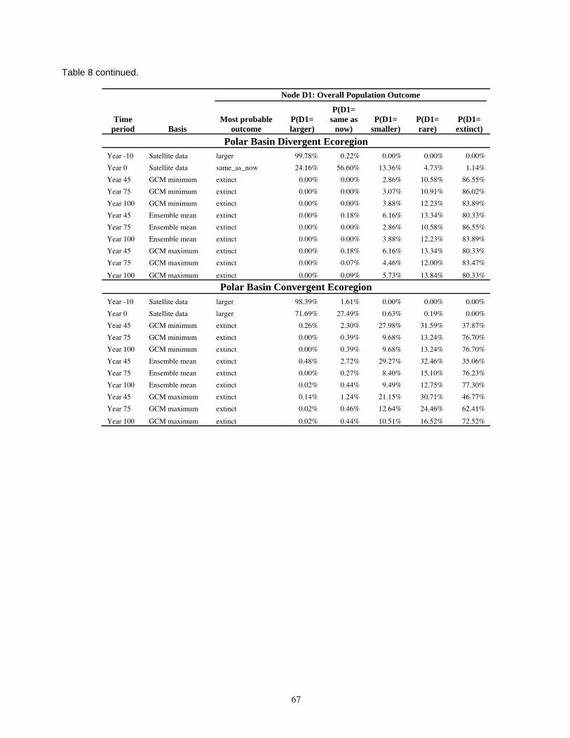
Table 8 continued.

Node D1: Overall Population Outcome

Time period Basis

Most probable outcome

P(D1= larger)

P(D1= same as

now) P(D1=

smaller) P(D1= rare)

P(D1= extinct)

Polar Basin Divergent Ecoregion Year -10 Satellite data larger 99.78% 0.22% 0.00% 0.00% 0.00%

Year 0 Satellite data same_as_now 24.16% 56.60% 13.36% 4.73% 1.14%

Year 45 GCM minimum extinct 0.00% 0.00% 2.86% 10.58% 86.55%

Year 75 GCM minimum extinct 0.00% 0.00% 3.07% 10.91% 86.02%

Year 100 GCM minimum extinct 0.00% 0.00% 3.88% 12.23% 83.89%

Year 45 Ensemble mean extinct 0.00% 0.18% 6.16% 13.34% 80.33%

Year 75 Ensemble mean extinct 0.00% 0.00% 2.86% 10.58% 86.55%

Year 100 Ensemble mean extinct 0.00% 0.00% 3.88% 12.23% 83.89%

Year 45 GCM maximum extinct 0.00% 0.18% 6.16% 13.34% 80.33%

Year 75 GCM maximum extinct 0.00% 0.07% 4.46% 12.00% 83.47%

Year 100 GCM maximum extinct 0.00% 0.09% 5.73% 13.84% 80.33%

Polar Basin Convergent Ecoregion Year -10 Satellite data larger 98.39% 1.61% 0.00% 0.00% 0.00%

Year 0 Satellite data larger 71.69% 27.49% 0.63% 0.19% 0.00%

Year 45 GCM minimum extinct 0.26% 2.30% 27.98% 31.59% 37.87%

Year 75 GCM minimum extinct 0.00% 0.39% 9.68% 13.24% 76.70%

Year 100 GCM minimum extinct 0.00% 0.39% 9.68% 13.24% 76.70%

Year 45 Ensemble mean extinct 0.48% 2.72% 29.27% 32.46% 35.06%

Year 75 Ensemble mean extinct 0.00% 0.27% 8.40% 15.10% 76.23%

Year 100 Ensemble mean extinct 0.02% 0.44% 9.49% 12.75% 77.30%

Year 45 GCM maximum extinct 0.14% 1.24% 21.15% 30.71% 46.77%

Year 75 GCM maximum extinct 0.02% 0.46% 12.64% 24.46% 62.41%

Year 100 GCM maximum extinct 0.02% 0.44% 10.51% 16.52% 72.52%

67

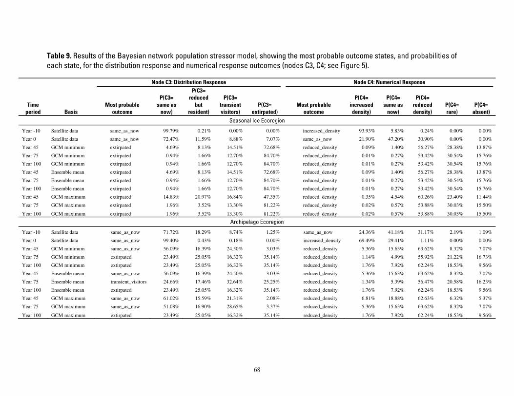
Table 9. Results of the Bayesian network population stressor model, showing the most probable outcome states, and probabilities of each state, for the distribution response and numerical response outcomes (nodes C3, C4; see Figure 5).

Node C3: Distribution Response Node C4: Numerical Response P(C3=

P(C3= reduced P(C3= P(C4= P(C4= P(C4= Time Most probable same as but transient P(C3= Most probable increased same as reduced P(C4= P(C4=

period Basis outcome now) resident) visitors) extirpated) outcome density) now) density) rare) absent) Seasonal Ice Ecoregion

Year -10 Satellite data same_as_now 99.79% 0.21% 0.00% 0.00% increased_density 93.93% 5.83% 0.24% 0.00% 0.00%

Year 0 Satellite data same_as_now 72.47% 11.59% 8.88% 7.07% same_as_now 21.90% 47.20% 30.90% 0.00% 0.00%

Year 45 GCM minimum extirpated 4.69% 8.13% 14.51% 72.68% reduced_density 0.09% 1.40% 56.27% 28.38% 13.87%

Year 75 GCM minimum extirpated 0.94% 1.66% 12.70% 84.70% reduced_density 0.01% 0.27% 53.42% 30.54% 15.76%

Year 100 GCM minimum extirpated 0.94% 1.66% 12.70% 84.70% reduced_density 0.01% 0.27% 53.42% 30.54% 15.76%

Year 45 Ensemble mean extirpated 4.69% 8.13% 14.51% 72.68% reduced_density 0.09% 1.40% 56.27% 28.38% 13.87%

Year 75 Ensemble mean extirpated 0.94% 1.66% 12.70% 84.70% reduced_density 0.01% 0.27% 53.42% 30.54% 15.76%

Year 100 Ensemble mean extirpated 0.94% 1.66% 12.70% 84.70% reduced_density 0.01% 0.27% 53.42% 30.54% 15.76%

Year 45 GCM maximum extirpated 14.83% 20.97% 16.84% 47.35% reduced_density 0.35% 4.54% 60.26% 23.40% 11.44%

Year 75 GCM maximum extirpated 1.96% 3.52% 13.30% 81.22% reduced_density 0.02% 0.57% 53.88% 30.03% 15.50%

Year 100 GCM maximum extirpated 1.96% 3.52% 13.30% 81.22% reduced_density 0.02% 0.57% 53.88% 30.03% 15.50%

Archipelago Ecoregion

Year -10 Satellite data same_as_now 71.72% 18.29% 8.74% 1.25% same_as_now 24.36% 41.18% 31.17% 2.19% 1.09%

Year 0 Satellite data same_as_now 99.40% 0.43% 0.18% 0.00% increased_density 69.49% 29.41% 1.11% 0.00% 0.00%

Year 45 GCM minimum same_as_now 56.09% 16.39% 24.50% 3.03% reduced_density 5.36% 15.63% 63.62% 8.32% 7.07%

Year 75 GCM minimum extirpated 23.49% 25.05% 16.32% 35.14% reduced_density 1.14% 4.99% 55.92% 21.22% 16.73%

Year 100 GCM minimum extirpated 23.49% 25.05% 16.32% 35.14% reduced_density 1.76% 7.92% 62.24% 18.53% 9.56%

Year 45 Ensemble mean same_as_now 56.09% 16.39% 24.50% 3.03% reduced_density 5.36% 15.63% 63.62% 8.32% 7.07%

Year 75 Ensemble mean transient_visitors 24.66% 17.46% 32.64% 25.25% reduced_density 1.34% 5.39% 56.47% 20.58% 16.23%

Year 100 Ensemble mean extirpated 23.49% 25.05% 16.32% 35.14% reduced_density 1.76% 7.92% 62.24% 18.53% 9.56%

Year 45 GCM maximum same_as_now 61.02% 15.59% 21.31% 2.08% reduced_density 6.81% 18.88% 62.63% 6.32% 5.37%

Year 75 GCM maximum same_as_now 51.08% 16.90% 28.65% 3.37% reduced_density 5.36% 15.63% 63.62% 8.32% 7.07%

Year 100 GCM maximum extirpated 23.49% 25.05% 16.32% 35.14% reduced_density 1.76% 7.92% 62.24% 18.53% 9.56%

68

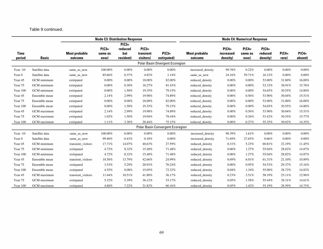
Table 9 continued.

Node C3: Distribution Response Node C4: Numerical Response P(C3=

P(C3= reduced P(C3= P(C4= P(C4= P(C4= Time Most probable same as but transient P(C3= Most probable increased same as reduced P(C4= P(C4=

period Basis outcome now) resident) visitors) extirpated) outcome density) now) density) rare) absent) Polar Basin Divergent Ecoregion

Year -10 Satellite data same_as_now 100.00% 0.00% 0.00% 0.00% increased_density 99.78% 0.22% 0.00% 0.00% 0.00%

Year 0 Satellite data same_as_now 85.66% 8.37% 4.82% 1.14% same_as_now 24.16% 59.71% 16.12% 0.00% 0.00%

Year 45 GCM minimum extirpated 0.00% 0.00% 18.00% 82.00% reduced_density 0.00% 0.00% 53.00% 31.00% 16.00%

Year 75 GCM minimum extirpated 0.00% 0.30% 18.27% 81.43% reduced_density 0.00% 0.00% 53.33% 30.91% 15.76%

Year 100 GCM minimum extirpated 0.00% 1.50% 19.35% 79.15% reduced_density 0.00% 0.00% 54.65% 30.55% 14.80%

Year 45 Ensemble mean extirpated 2.14% 2.99% 19.98% 74.89% reduced_density 0.00% 0.56% 53.90% 30.04% 15.51%

Year 75 Ensemble mean extirpated 0.00% 0.00% 18.00% 82.00% reduced_density 0.00% 0.00% 53.00% 31.00% 16.00%

Year 100 Ensemble mean extirpated 0.00% 1.50% 19.35% 79.15% reduced_density 0.00% 0.00% 54.65% 30.55% 14.80%

Year 45 GCM maximum extirpated 2.14% 2.99% 19.98% 74.89% reduced_density 0.00% 0.56% 53.90% 30.04% 15.51%

Year 75 GCM maximum extirpated 1.02% 1.50% 19.04% 78.44% reduced_density 0.00% 0.26% 53.42% 30.55% 15.77%

Year 100 GCM maximum extirpated 1.11% 3.30% 20.44% 75.15% reduced_density 0.00% 0.27% 55.35% 30.02% 14.35%

Polar Basin Convergent Ecoregion

Year -10 Satellite data same_as_now 100.00% 0.00% 0.00% 0.00% increased_density 98.39% 1.61% 0.00% 0.00% 0.00%

Year 0 Satellite data same_as_now 99.40% 0.43% 0.18% 0.00% increased_density 71.69% 27.65% 0.66% 0.00% 0.00%

Year 45 GCM minimum transient_visitors 17.71% 14.07% 40.63% 27.59% reduced_density 0.31% 5.23% 60.81% 22.19% 11.45%

Year 75 GCM minimum extirpated 4.72% 8.32% 15.48% 71.48% reduced_density 0.00% 1.27% 55.04% 28.82% 14.87%

Year 100 GCM minimum extirpated 4.72% 8.32% 15.48% 71.48% reduced_density 0.00% 1.27% 55.04% 28.82% 14.87%

Year 45 Ensemble mean transient_visitors 18.56% 13.79% 42.66% 24.99% reduced_density 0.69% 6.01% 61.31% 21.10% 10.89%

Year 75 Ensemble mean extirpated 3.53% 5.29% 20.93% 70.24% reduced_density 0.00% 0.95% 54.53% 29.37% 15.16%

Year 100 Ensemble mean extirpated 4.55% 8.08% 15.05% 72.32% reduced_density 0.04% 1.34% 55.08% 28.72% 14.82%

Year 45 GCM maximum transient_visitors 11.44% 10.51% 41.88% 36.17% reduced_density 0.23% 3.51% 58.19% 25.11% 12.96%

Year 75 GCM maximum extirpated 5.32% 5.39% 36.12% 53.17% reduced_density 0.05% 1.58% 55.44% 28.31% 14.61%

Year 100 GCM maximum extirpated 4.80% 7.22% 21.82% 66.16% reduced_density 0.05% 1.42% 55.19% 28.59% 14.75%

69

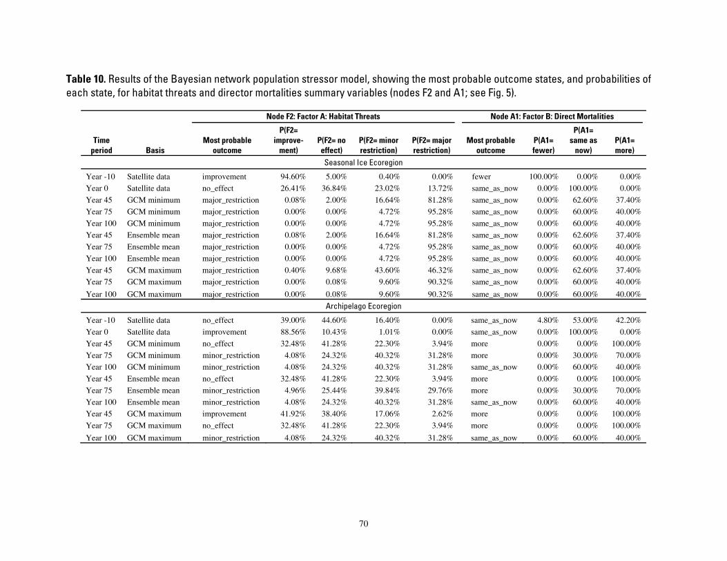
Table 10. Results of the Bayesian network population stressor model, showing the most probable outcome states, and probabilities of each state, for habitat threats and director mortalities summary variables (nodes F2 and A1; see Fig. 5).

Node F2: Factor A: Habitat Threats Node A1: Factor B: Direct Mortalities

P(F2= P(A1= Time Most probable improve­ P(F2= no P(F2= minor P(F2= major Most probable P(A1= same as P(A1=

period Basis outcome ment) effect) restriction) restriction) outcome fewer) now) more) Seasonal Ice Ecoregion

Year -10 Satellite data improvement 94.60% 5.00% 0.40% 0.00% fewer 100.00% 0.00% 0.00% Year 0 Satellite data no_effect 26.41% 36.84% 23.02% 13.72% same_as_now 0.00% 100.00% 0.00% Year 45 GCM minimum major_restriction 0.08% 2.00% 16.64% 81.28% same_as_now 0.00% 62.60% 37.40% Year 75 GCM minimum major_restriction 0.00% 0.00% 4.72% 95.28% same_as_now 0.00% 60.00% 40.00% Year 100 GCM minimum major_restriction 0.00% 0.00% 4.72% 95.28% same_as_now 0.00% 60.00% 40.00% Year 45 Ensemble mean major_restriction 0.08% 2.00% 16.64% 81.28% same_as_now 0.00% 62.60% 37.40% Year 75 Ensemble mean major_restriction 0.00% 0.00% 4.72% 95.28% same_as_now 0.00% 60.00% 40.00% Year 100 Ensemble mean major_restriction 0.00% 0.00% 4.72% 95.28% same_as_now 0.00% 60.00% 40.00% Year 45 GCM maximum major_restriction 0.40% 9.68% 43.60% 46.32% same_as_now 0.00% 62.60% 37.40% Year 75 GCM maximum major_restriction 0.00% 0.08% 9.60% 90.32% same_as_now 0.00% 60.00% 40.00%

Year 100 GCM maximum major_restriction 0.00% 0.08% 9.60% 90.32% same_as_now 0.00% 60.00% 40.00%

Archipelago Ecoregion

Year -10 Satellite data no_effect 39.00% 44.60% 16.40% 0.00% same_as_now 4.80% 53.00% 42.20% Year 0 Satellite data improvement 88.56% 10.43% 1.01% 0.00% same_as_now 0.00% 100.00% 0.00% Year 45 GCM minimum no_effect 32.48% 41.28% 22.30% 3.94% more 0.00% 0.00% 100.00% Year 75 GCM minimum minor_restriction 4.08% 24.32% 40.32% 31.28% more 0.00% 30.00% 70.00% Year 100 GCM minimum minor_restriction 4.08% 24.32% 40.32% 31.28% same_as_now 0.00% 60.00% 40.00% Year 45 Ensemble mean no_effect 32.48% 41.28% 22.30% 3.94% more 0.00% 0.00% 100.00% Year 75 Ensemble mean minor_restriction 4.96% 25.44% 39.84% 29.76% more 0.00% 30.00% 70.00% Year 100 Ensemble mean minor_restriction 4.08% 24.32% 40.32% 31.28% same_as_now 0.00% 60.00% 40.00% Year 45 GCM maximum improvement 41.92% 38.40% 17.06% 2.62% more 0.00% 0.00% 100.00% Year 75 GCM maximum no_effect 32.48% 41.28% 22.30% 3.94% more 0.00% 0.00% 100.00%

Year 100 GCM maximum minor_restriction 4.08% 24.32% 40.32% 31.28% same_as_now 0.00% 60.00% 40.00%

70

Table 10 continued.

Node F2: Factor A: Habitat Threats Node A1: Factor B: Direct Mortalities

P(F2= P(A1= Time Most probable improve­ P(F2= no P(F2= minor P(F2= major Most probable P(A1= same as

period Basis outcome ment) effect) restriction) restriction) outcome fewer) now) P(A1= more) Polar Basin Divergent Ecoregion

Year -10 Satellite data improvement 99.68% 0.32% 0.00% 0.00% fewer 100.00% 0.00% 0.00% Year 0 Satellite data no_effect 30.20% 47.24% 20.54% 2.02% same_as_now 0.00% 100.00% 0.00% Year 45 GCM minimum major_restriction 0.00% 0.00% 0.00% 100.00% same_as_now 0.00% 60.00% 40.00% Year 75 GCM minimum major_restriction 0.00% 0.00% 0.00% 100.00% same_as_now 0.00% 60.60% 39.40% Year 100 GCM minimum major_restriction 0.00% 0.00% 0.00% 100.00% same_as_now 0.00% 63.00% 37.00% Year 45 Ensemble mean major_restriction 0.00% 0.36% 9.80% 89.84% same_as_now 0.00% 60.00% 40.00% Year 75 Ensemble mean major_restriction 0.00% 0.00% 0.00% 100.00% same_as_now 0.00% 60.00% 40.00% Year 100 Ensemble mean major_restriction 0.00% 0.00% 0.00% 100.00% same_as_now 0.00% 63.00% 37.00% Year 45 GCM maximum major_restriction 0.00% 0.36% 9.80% 89.84% same_as_now 0.00% 60.00% 40.00% Year 75 GCM maximum major_restriction 0.00% 0.00% 5.08% 94.92% same_as_now 0.00% 60.00% 40.00%

Year 100 GCM maximum major_restriction 0.00% 0.00% 5.08% 94.92% same_as_now 0.00% 63.60% 36.40%

Polar Basin Convergent Ecoregion

Year -10 Satellite data improvement 97.48% 2.52% 0.00% 0.00% fewer 100.00% 0.00% 0.00% Year 0 Satellite data improvement 88.56% 10.43% 1.01% 0.00% same_as_now 0.00% 100.00% 0.00% Year 45 GCM minimum minor_restriction 1.10% 14.38% 48.19% 36.32% same_as_now 0.00% 60.00% 40.00% Year 75 GCM minimum major_restriction 0.00% 0.00% 23.60% 76.40% same_as_now 0.00% 60.00% 40.00% Year 100 GCM minimum major_restriction 0.00% 0.00% 23.60% 76.40% same_as_now 0.00% 60.00% 40.00% Year 45 Ensemble mean minor_restriction 1.25% 15.49% 49.10% 34.16% same_as_now 0.00% 60.00% 40.00% Year 75 Ensemble mean major_restriction 0.00% 0.00% 17.65% 82.35% same_as_now 0.00% 60.00% 40.00% Year 100 Ensemble mean major_restriction 0.00% 0.24% 22.16% 77.60% same_as_now 0.00% 60.00% 40.00% Year 45 GCM maximum major_restriction 0.29% 4.22% 45.49% 50.00% same_as_now 0.00% 60.00% 40.00% Year 75 GCM maximum major_restriction 0.00% 0.58% 25.18% 74.24% same_as_now 0.00% 60.00% 40.00%

Year 100 GCM maximum major_restriction 0.00% 0.35% 23.13% 76.52% same_as_now 0.00% 60.00% 40.00%

71

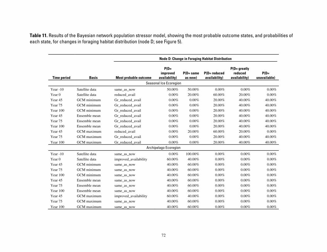
Table 11. Results of the Bayesian network population stressor model, showing the most probable outcome states, and probabilities of each state, for changes in foraging habitat distribution (node D; see Figure 5).

Node D: Change in Foraging Habitat Distribution

P(D= P(D= greatly improved P(D= same P(D= reduced reduced P(D=

Time period Basis Most probable outcome availability) as now) availability) availability) unavailable) Seasonal Ice Ecoregion

Year -10 Satellite data same_as_now 50.00% 50.00% 0.00% 0.00% 0.00% Year 0 Satellite data reduced_avail 0.00% 20.00% 60.00% 20.00% 0.00% Year 45 GCM minimum Gr_reduced_avail 0.00% 0.00% 20.00% 40.00% 40.00% Year 75 GCM minimum Gr_reduced_avail 0.00% 0.00% 20.00% 40.00% 40.00% Year 100 GCM minimum Gr_reduced_avail 0.00% 0.00% 20.00% 40.00% 40.00% Year 45 Ensemble mean Gr_reduced_avail 0.00% 0.00% 20.00% 40.00% 40.00% Year 75 Ensemble mean Gr_reduced_avail 0.00% 0.00% 20.00% 40.00% 40.00% Year 100 Ensemble mean Gr_reduced_avail 0.00% 0.00% 20.00% 40.00% 40.00% Year 45 GCM maximum reduced_avail 0.00% 20.00% 60.00% 20.00% 0.00% Year 75 GCM maximum Gr_reduced_avail 0.00% 0.00% 20.00% 40.00% 40.00%

Year 100 GCM maximum Gr_reduced_avail 0.00% 0.00% 20.00% 40.00% 40.00%

Archipelago Ecoregion

Year -10 Satellite data same_as_now 0.00% 100.00% 0.00% 0.00% 0.00% Year 0 Satellite data improved_availability 60.00% 40.00% 0.00% 0.00% 0.00% Year 45 GCM minimum same_as_now 40.00% 60.00% 0.00% 0.00% 0.00% Year 75 GCM minimum same_as_now 40.00% 60.00% 0.00% 0.00% 0.00% Year 100 GCM minimum same_as_now 40.00% 60.00% 0.00% 0.00% 0.00% Year 45 Ensemble mean same_as_now 40.00% 60.00% 0.00% 0.00% 0.00% Year 75 Ensemble mean same_as_now 40.00% 60.00% 0.00% 0.00% 0.00% Year 100 Ensemble mean same_as_now 40.00% 60.00% 0.00% 0.00% 0.00% Year 45 GCM maximum improved_availability 60.00% 40.00% 0.00% 0.00% 0.00% Year 75 GCM maximum same_as_now 40.00% 60.00% 0.00% 0.00% 0.00%

Year 100 GCM maximum same_as_now 40.00% 60.00% 0.00% 0.00% 0.00%

72

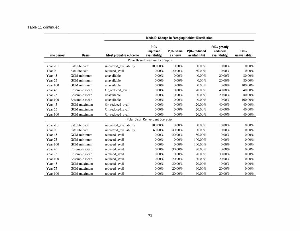
Table 11 continued.

Node D: Change in Foraging Habitat Distribution

P(D= P(D= greatly improved P(D= same P(D= reduced reduced P(D=

Time period Basis Most probable outcome availability) as now) availability) availability) unavailable) Polar Basin Divergent Ecoregion

Year -10 Satellite data improved_availability 100.00% 0.00% 0.00% 0.00% 0.00% Year 0 Satellite data reduced_avail 0.00% 20.00% 80.00% 0.00% 0.00% Year 45 GCM minimum unavailable 0.00% 0.00% 0.00% 20.00% 80.00% Year 75 GCM minimum unavailable 0.00% 0.00% 0.00% 20.00% 80.00% Year 100 GCM minimum unavailable 0.00% 0.00% 0.00% 0.00% 100.00% Year 45 Ensemble mean Gr_reduced_avail 0.00% 0.00% 20.00% 40.00% 40.00% Year 75 Ensemble mean unavailable 0.00% 0.00% 0.00% 20.00% 80.00% Year 100 Ensemble mean unavailable 0.00% 0.00% 0.00% 0.00% 100.00% Year 45 GCM maximum Gr_reduced_avail 0.00% 0.00% 20.00% 40.00% 40.00% Year 75 GCM maximum Gr_reduced_avail 0.00% 0.00% 20.00% 40.00% 40.00%

Year 100 GCM maximum Gr_reduced_avail 0.00% 0.00% 20.00% 40.00% 40.00%

Polar Basin Convergent Ecoregion

Year -10 Satellite data improved_availability 100.00% 0.00% 0.00% 0.00% 0.00% Year 0 Satellite data improved_availability 60.00% 40.00% 0.00% 0.00% 0.00% Year 45 GCM minimum reduced_avail 0.00% 20.00% 80.00% 0.00% 0.00% Year 75 GCM minimum reduced_avail 0.00% 0.00% 100.00% 0.00% 0.00% Year 100 GCM minimum reduced_avail 0.00% 0.00% 100.00% 0.00% 0.00% Year 45 Ensemble mean reduced_avail 0.00% 30.00% 70.00% 0.00% 0.00% Year 75 Ensemble mean reduced_avail 0.00% 0.00% 70.00% 30.00% 0.00% Year 100 Ensemble mean reduced_avail 0.00% 20.00% 60.00% 20.00% 0.00% Year 45 GCM maximum reduced_avail 0.00% 30.00% 70.00% 0.00% 0.00% Year 75 GCM maximum reduced_avail 0.00% 20.00% 60.00% 20.00% 0.00%

Year 100 GCM maximum reduced_avail 0.00% 20.00% 60.00% 20.00% 0.00%

73

Table 12. Results of the Bayesian network population stressor model, showing the most probable outcome states, and probabilities of each state, for disease/predation and other disturbance factors variables (nodes A4, A6; see Figure 5).

Node A4: Factor C: Disease, predation Node A6: Factor E: Other factors (natural or man-made)

P(A4= P(A6= Most probable same as P(A4= Most probable improve­ P(A6= no P(A6= minor P(A6= major

Time period Basis outcome now) worse) outcome ment) effect) restriction) restriction) Seasonal Ice Ecoregion

Year -10 Satellite data same_as_now 100.00% 0.00% improvement 84.80% 15.20% 0.00% 0.00% Year 0 Satellite data same_as_now 100.00% 0.00% no_effect 0.00% 100.00% 0.00% 0.00% Year 45 GCM minimum worse 0.00% 100.00% major_restriction 0.00% 0.00% 13.00% 87.00% Year 75 GCM minimum worse 0.00% 100.00% major_restriction 0.00% 0.00% 0.00% 100.00% Year 100 GCM minimum worse 0.00% 100.00% major_restriction 0.00% 0.00% 0.00% 100.00% Year 45 Ensemble mean worse 0.00% 100.00% major_restriction 0.00% 0.00% 13.00% 87.00% Year 75 Ensemble mean worse 0.00% 100.00% major_restriction 0.00% 0.00% 0.00% 100.00% Year 100 Ensemble mean worse 0.00% 100.00% major_restriction 0.00% 0.00% 0.00% 100.00% Year 45 GCM maximum worse 0.00% 100.00% major_restriction 0.00% 0.00% 13.00% 87.00% Year 75 GCM maximum worse 0.00% 100.00% major_restriction 0.00% 0.00% 0.00% 100.00%

Year 100 GCM maximum worse 0.00% 100.00% major_restriction 0.00% 0.00% 0.00% 100.00%

Archipelago Ecoregion

Year -10 Satellite data same_as_now 100.00% 0.00% major_restriction 4.80% 20.00% 34.80% 40.40% Year 0 Satellite data same_as_now 100.00% 0.00% no_effect 0.00% 100.00% 0.00% 0.00% Year 45 GCM minimum worse 30.00% 70.00% major_restriction 0.00% 0.00% 28.00% 72.00% Year 75 GCM minimum worse 0.00% 100.00% major_restriction 0.00% 0.00% 0.00% 100.00% Year 100 GCM minimum worse 0.00% 100.00% major_restriction 0.00% 0.00% 0.00% 100.00% Year 45 Ensemble mean worse 30.00% 70.00% major_restriction 0.00% 0.00% 28.00% 72.00% Year 75 Ensemble mean worse 0.00% 100.00% major_restriction 0.00% 0.00% 0.00% 100.00% Year 100 Ensemble mean worse 0.00% 100.00% major_restriction 0.00% 0.00% 0.00% 100.00% Year 45 GCM maximum worse 30.00% 70.00% major_restriction 0.00% 0.00% 28.00% 72.00% Year 75 GCM maximum worse 30.00% 70.00% major_restriction 0.00% 0.00% 0.00% 100.00%

Year 100 GCM maximum worse 0.00% 100.00% major_restriction 0.00% 0.00% 0.00% 100.00%

74

Table 12 continued.

Node A4: Factor C: Disease, predation Node A6: Factor E: Other factors (natural or man-made)

P(A4= P(A6= Most probable same as P(A4= Most probable improve­ P(A6= no P(A6= minor P(A6= major

Time period Basis outcome now) worse) outcome ment) effect) restriction) restriction) Polar Basin Divergent Ecoregion

Year -10 Satellite data same_as_now 100.00% 0.00% improvement 100.00% 0.00% 0.00% 0.00% Year 0 Satellite data same_as_now 100.00% 0.00% no_effect 0.00% 100.00% 0.00% 0.00% Year 45 GCM minimum worse 0.00% 100.00% major_restriction 0.00% 0.00% 0.00% 100.00% Year 75 GCM minimum worse 0.00% 100.00% major_restriction 0.00% 0.00% 3.00% 97.00% Year 100 GCM minimum worse 0.00% 100.00% major_restriction 0.00% 0.00% 15.00% 85.00% Year 45 Ensemble mean worse 0.00% 100.00% major_restriction 0.00% 0.00% 0.00% 100.00% Year 75 Ensemble mean worse 0.00% 100.00% major_restriction 0.00% 0.00% 0.00% 100.00% Year 100 Ensemble mean worse 0.00% 100.00% major_restriction 0.00% 0.00% 15.00% 85.00% Year 45 GCM maximum worse 0.00% 100.00% major_restriction 0.00% 0.00% 0.00% 100.00% Year 75 GCM maximum worse 0.00% 100.00% major_restriction 0.00% 0.00% 0.00% 100.00%

Year 100 GCM maximum worse 0.00% 100.00% major_restriction 0.00% 0.00% 18.00% 82.00%

Polar Basin Convergent Ecoregion

Year -10 Satellite data same_as_now 100.00% 0.00% improvement 100.00% 0.00% 0.00% 0.00% Year 0 Satellite data same_as_now 100.00% 0.00% no_effect 0.00% 100.00% 0.00% 0.00% Year 45 GCM minimum worse 0.00% 100.00% major_restriction 0.00% 0.00% 0.00% 100.00% Year 75 GCM minimum worse 0.00% 100.00% major_restriction 0.00% 0.00% 0.00% 100.00% Year 100 GCM minimum worse 0.00% 100.00% major_restriction 0.00% 0.00% 0.00% 100.00% Year 45 Ensemble mean worse 0.00% 100.00% major_restriction 0.00% 0.00% 0.00% 100.00% Year 75 Ensemble mean worse 0.00% 100.00% major_restriction 0.00% 0.00% 0.00% 100.00% Year 100 Ensemble mean worse 0.00% 100.00% major_restriction 0.00% 0.00% 0.00% 100.00% Year 45 GCM maximum worse 0.00% 100.00% major_restriction 0.00% 0.00% 0.00% 100.00% Year 75 GCM maximum worse 0.00% 100.00% major_restriction 0.00% 0.00% 0.00% 100.00%

Year 100 GCM maximum worse 0.00% 100.00% major_restriction 0.00% 0.00% 0.00% 100.00%

75

Table 13. Results of the Bayesian network population stressor model, showing the most probable outcome states, and probabilities of each state, for reproduction and vital rates (nodes U, L2; see Figure 5).

Node U: Reproduction Node L2: Vital Rates

P(L2= Most probable P(U= P(U= same P(U= Most probable P(L2 same as P(L2=

Time period Basis outcome increased) as now) decreased) outcome =improve) now) decline) Seasonal Ice Ecoregion

Year -10 Satellite data increased 59.68% 33.42% 6.90% improve 92.53% 7.00% 0.47% Year 0 Satellite data same_as_now 25.59% 41.59% 32.82% same_as_now 27.38% 41.72% 30.90% Year 45 GCM minimum decreased 1.78% 23.47% 74.75% decline 0.25% 7.04% 92.71% Year 75 GCM minimum decreased 0.38% 20.76% 78.87% decline 0.03% 1.47% 98.50% Year 100 GCM minimum decreased 0.38% 20.76% 78.87% decline 0.03% 1.47% 98.50% Year 45 Ensemble mean decreased 1.78% 23.47% 74.75% decline 0.25% 7.04% 92.71% Year 75 Ensemble mean decreased 0.38% 20.76% 78.87% decline 0.03% 1.47% 98.50% Year 100 Ensemble mean decreased 0.38% 20.76% 78.87% decline 0.03% 1.47% 98.50% Year 45 GCM maximum decreased 5.67% 30.90% 63.43% decline 1.01% 22.54% 76.45% Year 75 GCM maximum decreased 0.78% 21.57% 77.65% decline 0.05% 3.07% 96.87%

Year 100 GCM maximum decreased 0.78% 21.57% 77.65% decline 0.05% 3.07% 96.87%

Archipelago Ecoregion

Year -10 Satellite data same_as_now 34.41% 45.14% 20.44% same_as_now 39.94% 47.09% 12.97% Year 0 Satellite data increased 57.07% 34.96% 7.96% improve 86.86% 12.04% 1.11% Year 45 GCM minimum same_as_now 30.18% 43.98% 25.84% same_as_now 33.47% 45.72% 20.80% Year 75 GCM minimum decreased 10.62% 36.67% 52.71% decline 5.17% 35.07% 59.76% Year 100 GCM minimum decreased 10.62% 36.67% 52.71% decline 5.17% 35.07% 59.76% Year 45 Ensemble mean same_as_now 30.18% 43.98% 25.84% same_as_now 33.47% 45.72% 20.80% Year 75 Ensemble mean decreased 11.35% 37.15% 51.50% decline 6.07% 35.97% 57.96% Year 100 Ensemble mean decreased 10.62% 36.67% 52.71% decline 5.17% 35.07% 59.76% Year 45 GCM maximum same_as_now 35.03% 43.12% 21.85% improve 42.54% 41.66% 15.80% Year 75 GCM maximum same_as_now 30.18% 43.98% 25.84% same_as_now 33.47% 45.72% 20.80%

Year 100 GCM maximum decreased 10.62% 36.67% 52.71% decline 5.17% 35.07% 59.76%

76

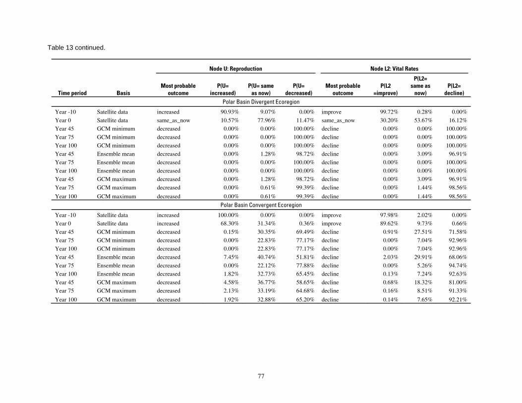
Table 13 continued.

Node U: Reproduction Node L2: Vital Rates

P(L2= Most probable P(U= P(U= same P(U= Most probable P(L2 same as P(L2=

Time period Basis outcome increased) as now) decreased) outcome =improve) now) decline) Polar Basin Divergent Ecoregion

Year -10 Satellite data increased 90.93% 9.07% 0.00% improve 99.72% 0.28% 0.00% Year 0 Satellite data same_as_now 10.57% 77.96% 11.47% same_as_now 30.20% 53.67% 16.12% Year 45 GCM minimum decreased 0.00% 0.00% 100.00% decline 0.00% 0.00% 100.00% Year 75 GCM minimum decreased 0.00% 0.00% 100.00% decline 0.00% 0.00% 100.00% Year 100 GCM minimum decreased 0.00% 0.00% 100.00% decline 0.00% 0.00% 100.00% Year 45 Ensemble mean decreased 0.00% 1.28% 98.72% decline 0.00% 3.09% 96.91% Year 75 Ensemble mean decreased 0.00% 0.00% 100.00% decline 0.00% 0.00% 100.00% Year 100 Ensemble mean decreased 0.00% 0.00% 100.00% decline 0.00% 0.00% 100.00% Year 45 GCM maximum decreased 0.00% 1.28% 98.72% decline 0.00% 3.09% 96.91% Year 75 GCM maximum decreased 0.00% 0.61% 99.39% decline 0.00% 1.44% 98.56%

Year 100 GCM maximum decreased 0.00% 0.61% 99.39% decline 0.00% 1.44% 98.56%

Polar Basin Convergent Ecoregion

Year -10 Satellite data increased 100.00% 0.00% 0.00% improve 97.98% 2.02% 0.00% Year 0 Satellite data increased 68.30% 31.34% 0.36% improve 89.62% 9.73% 0.66% Year 45 GCM minimum decreased 0.15% 30.35% 69.49% decline 0.91% 27.51% 71.58% Year 75 GCM minimum decreased 0.00% 22.83% 77.17% decline 0.00% 7.04% 92.96% Year 100 GCM minimum decreased 0.00% 22.83% 77.17% decline 0.00% 7.04% 92.96% Year 45 Ensemble mean decreased 7.45% 40.74% 51.81% decline 2.03% 29.91% 68.06% Year 75 Ensemble mean decreased 0.00% 22.12% 77.88% decline 0.00% 5.26% 94.74% Year 100 Ensemble mean decreased 1.82% 32.73% 65.45% decline 0.13% 7.24% 92.63% Year 45 GCM maximum decreased 4.58% 36.77% 58.65% decline 0.68% 18.32% 81.00% Year 75 GCM maximum decreased 2.13% 33.19% 64.68% decline 0.16% 8.51% 91.33%

Year 100 GCM maximum decreased 1.92% 32.88% 65.20% decline 0.14% 7.65% 92.21%

77

Table 14. Projected outcomes from Bayesian network population stressor model showing probabilities of overall outcome states resulting when all human factors were fixed at ‘same as now’ or ‘fewer than now.’

"Influence Run" #1 "Influence Run" #2

Outcome forcing Node A1 = "same as now" and Outcome forcing Node A1 = "fewer" and Node A6 = "no effect", for Years 45, 75, 100 Node A6 = "improvement", for Years 45, 75, 100

Node D1: Overall Population Outcome Node D1: Overall Population Outcome

Time P(D1= P(D1= same P(D1= P(D1= P(D1= P(D1= P(D1= same P(D1= P(D1= P(D1= period Basis most-prob D1 larger) as now) smaller) rare) extinct) most-prob D1 larger) as now) smaller) rare) extinct)

Seasonal Ice Ecoregion

Year -10 Satellite data larger 93.92% 5.75% 0.30% 0.02% 0.00% larger 93.92% 5.75% 0.30% 0.02% 0.00% Year 0 Satellite data same_as_now 21.85% 43.72% 18.98% 8.37% 7.07% same_as_now 21.85% 43.72% 18.98% 8.37% 7.07% Year 45 GCM minimum extinct 0.10% 1.46% 22.80% 21.20% 54.40% extinct 0.11% 8.43% 31.70% 14.00% 45.80% Year 75 GCM minimum extinct 0.01% 0.24% 16.20% 20.20% 63.30% extinct 0.01% 3.89% 27.90% 14.70% 53.50% Year 100 GCM minimum extinct 0.01% 0.52% 18.60% 18.70% 62.20% extinct 0.10% 4.98% 28.10% 13.30% 53.50% Year 45 Ensemble mean extinct 0.10% 1.46% 22.80% 21.20% 54.40% extinct 0.11% 8.43% 31.70% 14.00% 45.80% Year 75 Ensemble mean extinct 0.01% 0.24% 16.20% 20.20% 63.30% extinct 0.01% 3.89% 27.90% 14.70% 53.50% Year 100 Ensemble mean extinct 0.01% 0.24% 16.20% 20.20% 63.30% extinct 0.01% 3.89% 27.90% 14.70% 53.50% Year 45 GCM maximum smaller 0.45% 5.16% 39.50% 22.80% 32.00% smaller 0.46% 21.10% 40.30% 11.90% 26.30% Year 75 GCM maximum extinct 0.02% 0.52% 18.50% 20.80% 60.20% extinct 0.02% 5.20% 29.50% 14.50% 50.80%

Year 100 GCM maximum extinct 0.02% 0.52% 18.50% 20.80% 60.20% extinct 0.02% 5.20% 29.50% 14.50% 50.80% Archipelago Ecoregion

Year -10 Satellite data same_as_now 22.51% 34.73% 31.48% 8.72% 2.56% same_as_now 22.51% 34.73% 31.48% 8.72% 2.56% Year 0 Satellite data larger 69.48% 29.26% 1.06% 0.19% 0.00% larger 69.48% 29.26% 1.06% 0.19% 0.00% Year 45 GCM minimum smaller 19.70% 29.40% 39.70% 8.90% 2.26% same_as_now 24.30% 44.10% 25.40% 4.62% 1.55% Year 75 GCM minimum smaller 2.54% 10.10% 46.40% 19.00% 22.00% smaller 2.55% 31.80% 38.50% 9.30% 17.80% Year 100 GCM minimum smaller 2.54% 10.10% 46.40% 19.00% 22.00% smaller 2.55% 31.80% 38.50% 9.30% 17.80% Year 45 Ensemble mean smaller 19.70% 29.40% 39.70% 8.90% 2.26% same_as_now 24.30% 44.10% 25.40% 4.62% 1.55% Year 75 Ensemble mean smaller 2.99% 10.50% 46.50% 23.50% 16.50% smaller 2.99% 32.10% 38.90% 13.20% 12.70% Year 100 Ensemble mean smaller 2.54% 10.10% 46.40% 19.00% 22.00% smaller 2.55% 31.80% 38.50% 9.30% 17.80% Year 45 GCM maximum smaller 25.10% 29.90% 36.80% 6.72% 1.55% same_as_now 30.00% 42.10% 23.40% 3.43% 1.03% Year 75 GCM maximum smaller 19.70% 29.40% 39.70% 8.90% 2.26% same_as_now 24.30% 44.10% 25.40% 4.62% 1.55% Year 100 GCM maximum smaller 2.54% 10.10% 46.40% 19.00% 22.00% smaller 2.55% 31.80% 38.50% 9.30% 17.80%

78

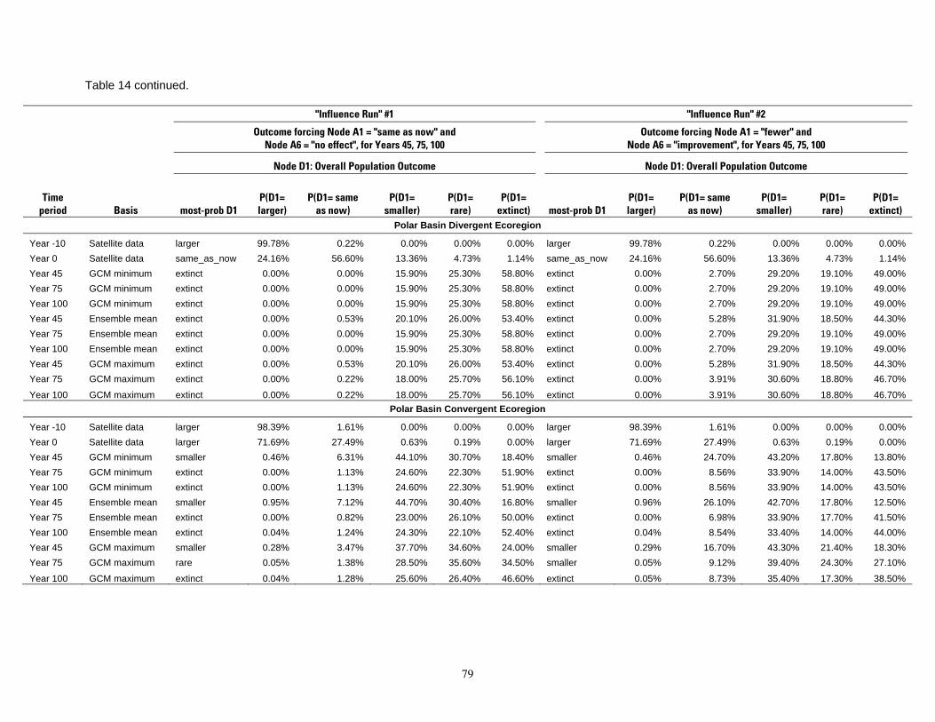
Table 14 continued.

"Influence Run" #1 "Influence Run" #2

Outcome forcing Node A1 = "same as now" and Outcome forcing Node A1 = "fewer" and Node A6 = "no effect", for Years 45, 75, 100 Node A6 = "improvement", for Years 45, 75, 100

Node D1: Overall Population Outcome Node D1: Overall Population Outcome

Time P(D1= P(D1= same P(D1= P(D1= P(D1= P(D1= P(D1= same P(D1= P(D1= P(D1= period Basis most-prob D1 larger) as now) smaller) rare) extinct) most-prob D1 larger) as now) smaller) rare) extinct)

Polar Basin Divergent Ecoregion

Year -10 Satellite data larger 99.78% 0.22% 0.00% 0.00% 0.00% larger 99.78% 0.22% 0.00% 0.00% 0.00% Year 0 Satellite data same_as_now 24.16% 56.60% 13.36% 4.73% 1.14% same_as_now 24.16% 56.60% 13.36% 4.73% 1.14% Year 45 GCM minimum extinct 0.00% 0.00% 15.90% 25.30% 58.80% extinct 0.00% 2.70% 29.20% 19.10% 49.00% Year 75 GCM minimum extinct 0.00% 0.00% 15.90% 25.30% 58.80% extinct 0.00% 2.70% 29.20% 19.10% 49.00% Year 100 GCM minimum extinct 0.00% 0.00% 15.90% 25.30% 58.80% extinct 0.00% 2.70% 29.20% 19.10% 49.00% Year 45 Ensemble mean extinct 0.00% 0.53% 20.10% 26.00% 53.40% extinct 0.00% 5.28% 31.90% 18.50% 44.30% Year 75 Ensemble mean extinct 0.00% 0.00% 15.90% 25.30% 58.80% extinct 0.00% 2.70% 29.20% 19.10% 49.00% Year 100 Ensemble mean extinct 0.00% 0.00% 15.90% 25.30% 58.80% extinct 0.00% 2.70% 29.20% 19.10% 49.00% Year 45 GCM maximum extinct 0.00% 0.53% 20.10% 26.00% 53.40% extinct 0.00% 5.28% 31.90% 18.50% 44.30% Year 75 GCM maximum extinct 0.00% 0.22% 18.00% 25.70% 56.10% extinct 0.00% 3.91% 30.60% 18.80% 46.70%

Year 100 GCM maximum extinct 0.00% 0.22% 18.00% 25.70% 56.10% extinct 0.00% 3.91% 30.60% 18.80% 46.70% Polar Basin Convergent Ecoregion

Year -10 Satellite data larger 98.39% 1.61% 0.00% 0.00% 0.00% larger 98.39% 1.61% 0.00% 0.00% 0.00% Year 0 Satellite data larger 71.69% 27.49% 0.63% 0.19% 0.00% larger 71.69% 27.49% 0.63% 0.19% 0.00% Year 45 GCM minimum smaller 0.46% 6.31% 44.10% 30.70% 18.40% smaller 0.46% 24.70% 43.20% 17.80% 13.80% Year 75 GCM minimum extinct 0.00% 1.13% 24.60% 22.30% 51.90% extinct 0.00% 8.56% 33.90% 14.00% 43.50% Year 100 GCM minimum extinct 0.00% 1.13% 24.60% 22.30% 51.90% extinct 0.00% 8.56% 33.90% 14.00% 43.50% Year 45 Ensemble mean smaller 0.95% 7.12% 44.70% 30.40% 16.80% smaller 0.96% 26.10% 42.70% 17.80% 12.50% Year 75 Ensemble mean extinct 0.00% 0.82% 23.00% 26.10% 50.00% extinct 0.00% 6.98% 33.90% 17.70% 41.50% Year 100 Ensemble mean extinct 0.04% 1.24% 24.30% 22.10% 52.40% extinct 0.04% 8.54% 33.40% 14.00% 44.00% Year 45 GCM maximum smaller 0.28% 3.47% 37.70% 34.60% 24.00% smaller 0.29% 16.70% 43.30% 21.40% 18.30% Year 75 GCM maximum rare 0.05% 1.38% 28.50% 35.60% 34.50% smaller 0.05% 9.12% 39.40% 24.30% 27.10%

Year 100 GCM maximum extinct 0.04% 1.28% 25.60% 26.40% 46.60% extinct 0.05% 8.73% 35.40% 17.30% 38.50%

79

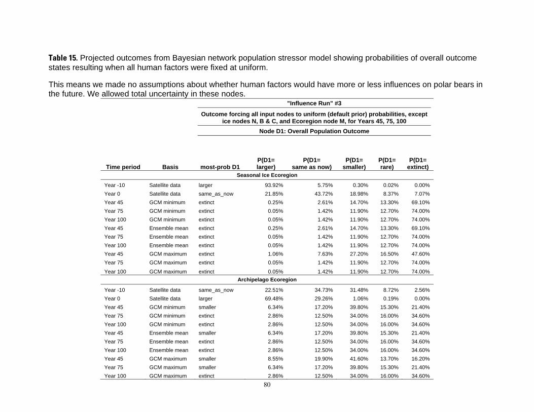
Table 15. Projected outcomes from Bayesian network population stressor model showing probabilities of overall outcome states resulting when all human factors were fixed at uniform.

This means we made no assumptions about whether human factors would have more or less influences on polar bears in the future. We allowed total uncertainty in these nodes.

"Influence Run" #3

Outcome forcing all input nodes to uniform (default prior) probabilities, except ice nodes N, B & C, and Ecoregion node M, for Years 45, 75, 100

Node D1: Overall Population Outcome

Time period Basis most-prob D1 P(D1= larger)

P(D1= same as now)

P(D1= smaller)

P(D1= rare)

P(D1= extinct)

Seasonal Ice Ecoregion

Year -10 Satellite data larger 93.92% 5.75% 0.30% 0.02% 0.00% Year 0 Satellite data same_as_now 21.85% 43.72% 18.98% 8.37% 7.07% Year 45 GCM minimum extinct 0.25% 2.61% 14.70% 13.30% 69.10% Year 75 GCM minimum extinct 0.05% 1.42% 11.90% 12.70% 74.00% Year 100 GCM minimum extinct 0.05% 1.42% 11.90% 12.70% 74.00% Year 45 Ensemble mean extinct 0.25% 2.61% 14.70% 13.30% 69.10% Year 75 Ensemble mean extinct 0.05% 1.42% 11.90% 12.70% 74.00% Year 100 Ensemble mean extinct 0.05% 1.42% 11.90% 12.70% 74.00% Year 45 GCM maximum extinct 1.06% 7.63% 27.20% 16.50% 47.60% Year 75 GCM maximum extinct 0.05% 1.42% 11.90% 12.70% 74.00%

Year 100 GCM maximum extinct 0.05% 1.42% 11.90% 12.70% 74.00% Archipelago Ecoregion

Year -10 Satellite data same_as_now 22.51% 34.73% 31.48% 8.72% 2.56% Year 0 Satellite data larger 69.48% 29.26% 1.06% 0.19% 0.00% Year 45 GCM minimum smaller 6.34% 17.20% 39.80% 15.30% 21.40% Year 75 GCM minimum extinct 2.86% 12.50% 34.00% 16.00% 34.60% Year 100 GCM minimum extinct 2.86% 12.50% 34.00% 16.00% 34.60% Year 45 Ensemble mean smaller 6.34% 17.20% 39.80% 15.30% 21.40% Year 75 Ensemble mean extinct 2.86% 12.50% 34.00% 16.00% 34.60% Year 100 Ensemble mean extinct 2.86% 12.50% 34.00% 16.00% 34.60% Year 45 GCM maximum smaller 8.55% 19.90% 41.60% 13.70% 16.20% Year 75 GCM maximum smaller 6.34% 17.20% 39.80% 15.30% 21.40% Year 100 GCM maximum extinct 2.86% 12.50% 34.00% 16.00% 34.60%

80

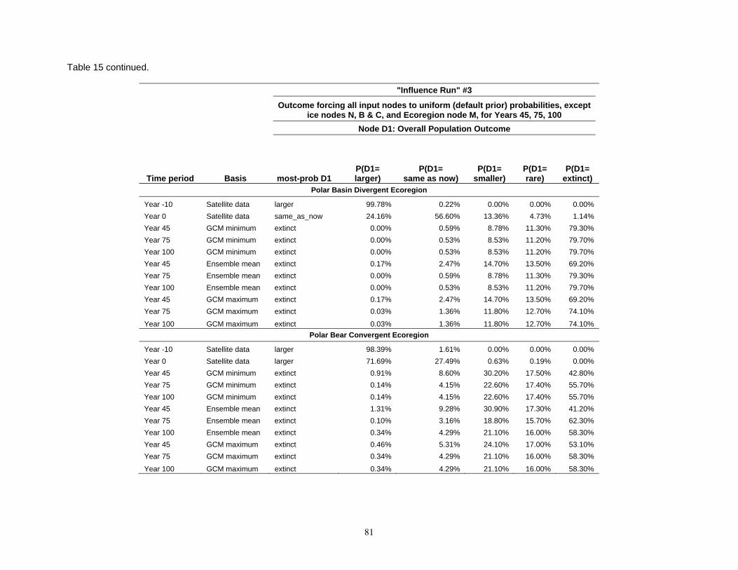
Table 15 continued.

"Influence Run" #3

Outcome forcing all input nodes to uniform (default prior) probabilities, except ice nodes N, B & C, and Ecoregion node M, for Years 45, 75, 100

Node D1: Overall Population Outcome

Time period Basis most-prob D1 P(D1= larger)

P(D1= same as now)

P(D1= smaller)

P(D1= rare)

P(D1= extinct)

Polar Basin Divergent Ecoregion

Year -10 Satellite data larger 99.78% 0.22% 0.00% 0.00% 0.00% Year 0 Satellite data same_as_now 24.16% 56.60% 13.36% 4.73% 1.14% Year 45 GCM minimum extinct 0.00% 0.59% 8.78% 11.30% 79.30% Year 75 GCM minimum extinct 0.00% 0.53% 8.53% 11.20% 79.70% Year 100 GCM minimum extinct 0.00% 0.53% 8.53% 11.20% 79.70% Year 45 Ensemble mean extinct 0.17% 2.47% 14.70% 13.50% 69.20% Year 75 Ensemble mean extinct 0.00% 0.59% 8.78% 11.30% 79.30% Year 100 Ensemble mean extinct 0.00% 0.53% 8.53% 11.20% 79.70% Year 45 GCM maximum extinct 0.17% 2.47% 14.70% 13.50% 69.20% Year 75 GCM maximum extinct 0.03% 1.36% 11.80% 12.70% 74.10%

Year 100 GCM maximum extinct 0.03% 1.36% 11.80% 12.70% 74.10% Polar Bear Convergent Ecoregion

Year -10 Satellite data larger 98.39% 1.61% 0.00% 0.00% 0.00% Year 0 Satellite data larger 71.69% 27.49% 0.63% 0.19% 0.00% Year 45 GCM minimum extinct 0.91% 8.60% 30.20% 17.50% 42.80% Year 75 GCM minimum extinct 0.14% 4.15% 22.60% 17.40% 55.70% Year 100 GCM minimum extinct 0.14% 4.15% 22.60% 17.40% 55.70% Year 45 Ensemble mean extinct 1.31% 9.28% 30.90% 17.30% 41.20% Year 75 Ensemble mean extinct 0.10% 3.16% 18.80% 15.70% 62.30% Year 100 Ensemble mean extinct 0.34% 4.29% 21.10% 16.00% 58.30% Year 45 GCM maximum extinct 0.46% 5.31% 24.10% 17.00% 53.10% Year 75 GCM maximum extinct 0.34% 4.29% 21.10% 16.00% 58.30%

Year 100 GCM maximum extinct 0.34% 4.29% 21.10% 16.00% 58.30%

81

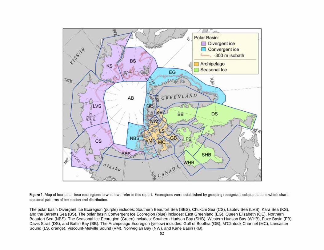
Figure 1. Map of four polar bear ecoregions to which we refer in this report. Ecoregions were established by grouping recognized subpopulations which share seasonal patterns of ice motion and distribution.

The polar basin Divergent Ice Ecoregion (purple) includes: Southern Beaufort Sea (SBS), Chukchi Sea (CS), Laptev Sea (LVS), Kara Sea (KS), and the Barents Sea (BS). The polar basin Convergent Ice Ecoregion (blue) includes: East Greenland (EG), Queen Elizabeth (QE), Northern Beaufort Sea (NBS). The Seasonal Ice Ecoregion (Green) includes: Southern Hudson Bay (SHB), Western Hudson Bay (WHB), Foxe Basin (FB), Davis Strait (DS), and Baffin Bay (BB). The Archipelago Ecoregion (yellow) includes: Gulf of Boothia (GB), M’Clintock Channel (MC), Lancaster Sound (LS, orange), Viscount-Melville Sound (VM), Norwegian Bay (NW), and Kane Basin (KB).

82

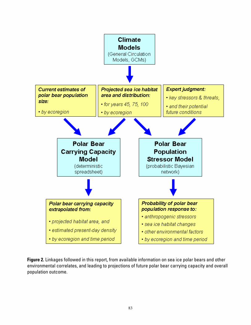
Figure 2. Linkages followed in this report, from available information on sea ice polar bears and other environmental correlates, and leading to projections of future polar bear carrying capacity and overall population outcome.

83

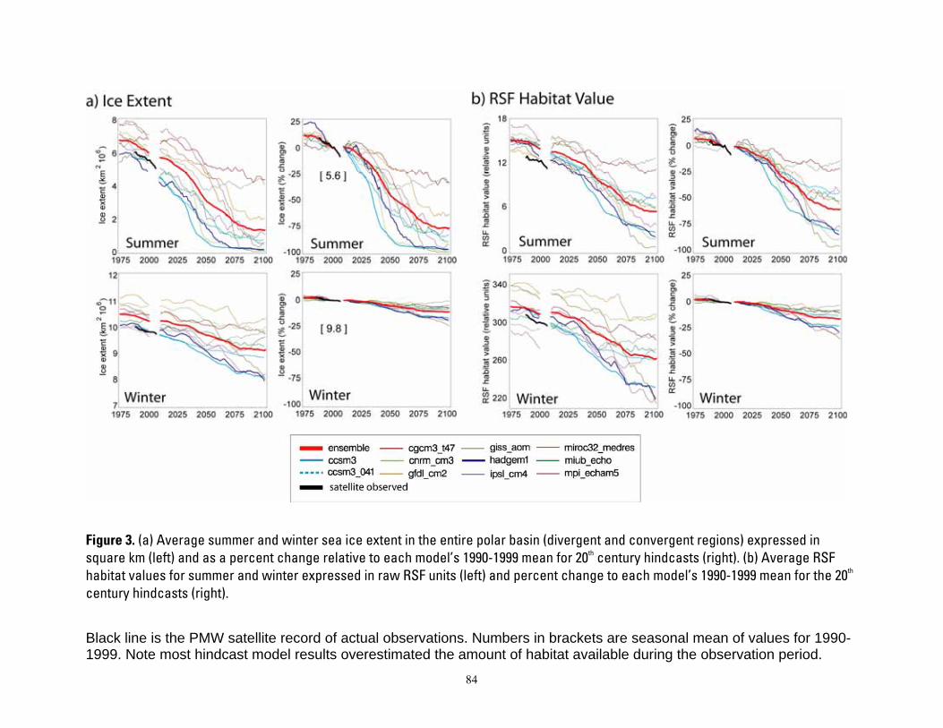
Figure 3. (a) Average summer and winter sea ice extent in the entire polar basin (divergent and convergent regions) expressed in square km (left) and as a percent change relative to each model’s 1990-1999 mean for 20th century hindcasts (right). (b) Average RSF habitat values for summer and winter expressed in raw RSF units (left) and percent change to each model’s 1990-1999 mean for the 20th

century hindcasts (right).

Black line is the PMW satellite record of actual observations. Numbers in brackets are seasonal mean of values for 1990-1999. Note most hindcast model results overestimated the amount of habitat available during the observation period.

84

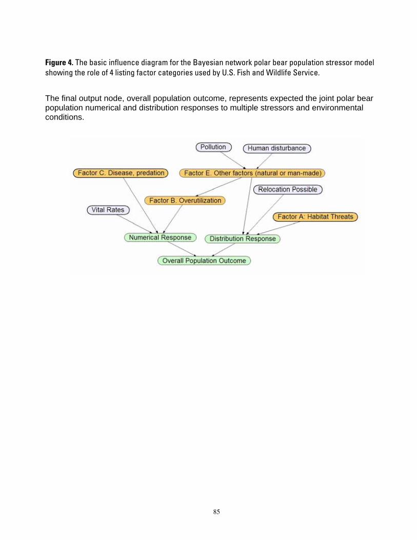
Figure 4. The basic influence diagram for the Bayesian network polar bear population stressor model showing the role of 4 listing factor categories used by U.S. Fish and Wildlife Service.

The final output node, overall population outcome, represents expected the joint polar bear population numerical and distribution responses to multiple stressors and environmental conditions.

85

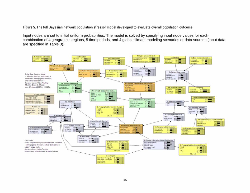
Figure 5. The full Bayesian network population stressor model developed to evaluate overall population outcome.

Input nodes are set to initial uniform probabilities. The model is solved by specifying input node values for each combination of 4 geographic regions, 5 time periods, and 4 global climate modeling scenarios or data sources (input data are specified in Table 3).

86

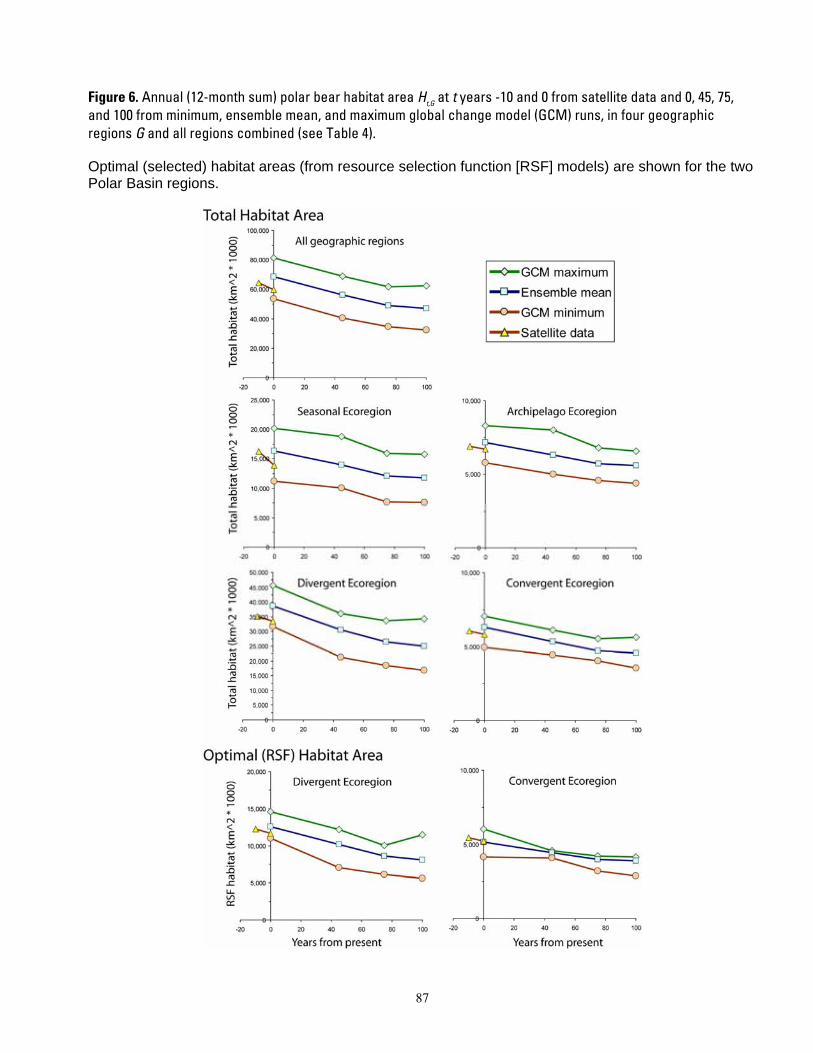
Figure 6. Annual (12-month sum) polar bear habitat area Ht,G at t years -10 and 0 from satellite data and 0, 45, 75, and 100 from minimum, ensemble mean, and maximum global change model (GCM) runs, in four geographic regions G and all regions combined (see Table 4).

Optimal (selected) habitat areas (from resource selection function [RSF] models) are shown for the two Polar Basin regions.

87

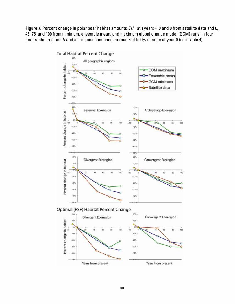
Figure 7. Percent change in polar bear habitat amounts CHt,G at t years -10 and 0 from satellite data and 0, 45, 75, and 100 from minimum, ensemble mean, and maximum global change model (GCM) runs, in four geographic regions G and all regions combined, normalized to 0% change at year 0 (see Table 4).

88

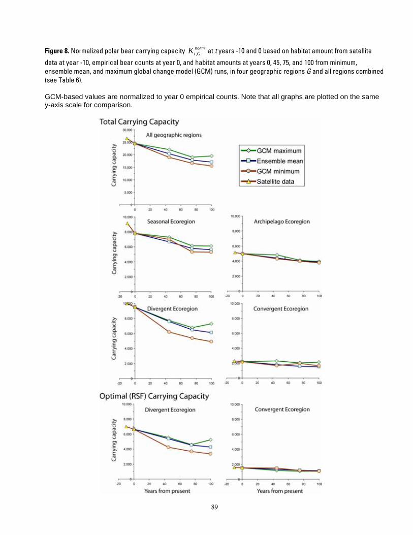
Figure 8. Normalized polar bear carrying capacity K norm at t years -10 and 0 based on habitat amount from satellite t ,G

data at year -10, empirical bear counts at year 0, and habitat amounts at years 0, 45, 75, and 100 from minimum, ensemble mean, and maximum global change model (GCM) runs, in four geographic regions G and all regions combined (see Table 6).

GCM-based values are normalized to year 0 empirical counts. Note that all graphs are plotted on the same y-axis scale for comparison.

89

Figure 9. Polar bear carrying capacity trends CKt,G at t years -10 and 0 based on carrying capacity values from Figure 8, in four geographic regions G and all regions combined, normalized to 0% change at year 0 (see Table 6).

90

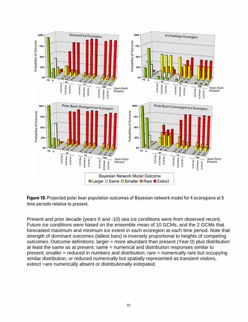
Figure 10. Projected polar bear population outcomes of Bayesian network model for 4 ecoregions at 5 time periods relative to present.

Present and prior decade (years 0 and -10) sea ice conditions were from observed record. Future ice conditions were based on the ensemble mean of 10 GCMs, and the 2 GCMs that forecasted maximum and minimum ice extent in each ecoregion at each time period. Note that strength of dominant outcomes (tallest bars) is inversely proportional to heights of competing outcomes. Outcome definitions: larger = more abundant than present (Year 0) plus distribution at least the same as at present; same = numerical and distribution responses similar to present; smaller = reduced in numbers and distribution; rare = numerically rare but occupying similar distribution, or reduced numerically but spatially represented as transient visitors, extinct =are numerically absent or distributionally extirpated.

91

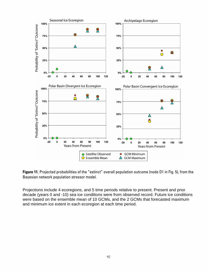
Figure 11. Projected probabilities of the “extinct” overall population outcome (node D1 in Fig. 5), from the Bayesian network population stressor model.

Projections include 4 ecoregions, and 5 time periods relative to present. Present and prior decade (years 0 and -10) sea ice conditions were from observed record. Future ice conditions were based on the ensemble mean of 10 GCMs, and the 2 GCMs that forecasted maximum and minimum ice extent in each ecoregion at each time period.

92

Figure 12. Cumulative sensitivity of overall population outcome (node D1, Fig. 5) to all input variables (yellow boxes, Fig. 5), in the Bayesian network population stressor model.

The 17 input variables on the vertical axis are listed, top to bottom, in decreasing order of their individual influence on overall population outcome (see Appendix 1, Sensitivity Test 1). The horizontal axis represents the cumulative proportion of total entropy reduction (mutual information) from the input variables. For example, the first two variables, foraging habitat quantity change and foraging habitat absence change, together account for 58% of all explainable entropy reduction.

93

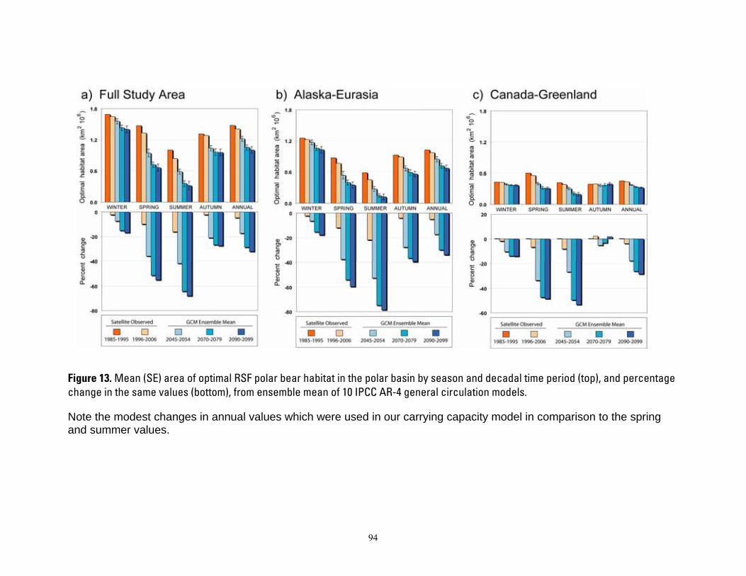
Figure 13. Mean (SE) area of optimal RSF polar bear habitat in the polar basin by season and decadal time period (top), and percentage change in the same values (bottom), from ensemble mean of 10 IPCC AR-4 general circulation models.

Note the modest changes in annual values which were used in our carrying capacity model in comparison to the spring and summer values.

94

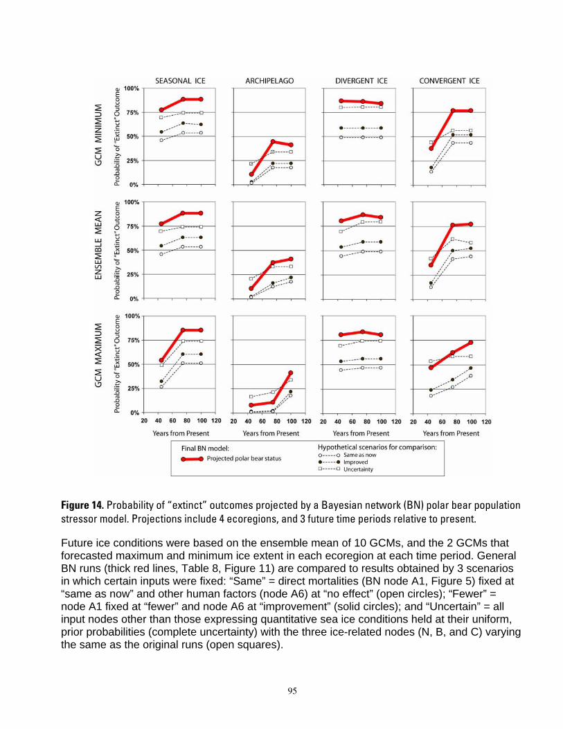
Figure 14. Probability of “extinct” outcomes projected by a Bayesian network (BN) polar bear population stressor model. Projections include 4 ecoregions, and 3 future time periods relative to present.

Future ice conditions were based on the ensemble mean of 10 GCMs, and the 2 GCMs that forecasted maximum and minimum ice extent in each ecoregion at each time period. General BN runs (thick red lines, Table 8, Figure 11) are compared to results obtained by 3 scenarios in which certain inputs were fixed: “Same” = direct mortalities (BN node A1, Figure 5) fixed at “same as now” and other human factors (node A6) at “no effect” (open circles); “Fewer” = node A1 fixed at “fewer” and node A6 at “improvement” (solid circles); and “Uncertain” = all input nodes other than those expressing quantitative sea ice conditions held at their uniform, prior probabilities (complete uncertainty) with the three ice-related nodes (N, B, and C) varying the same as the original runs (open squares).

95

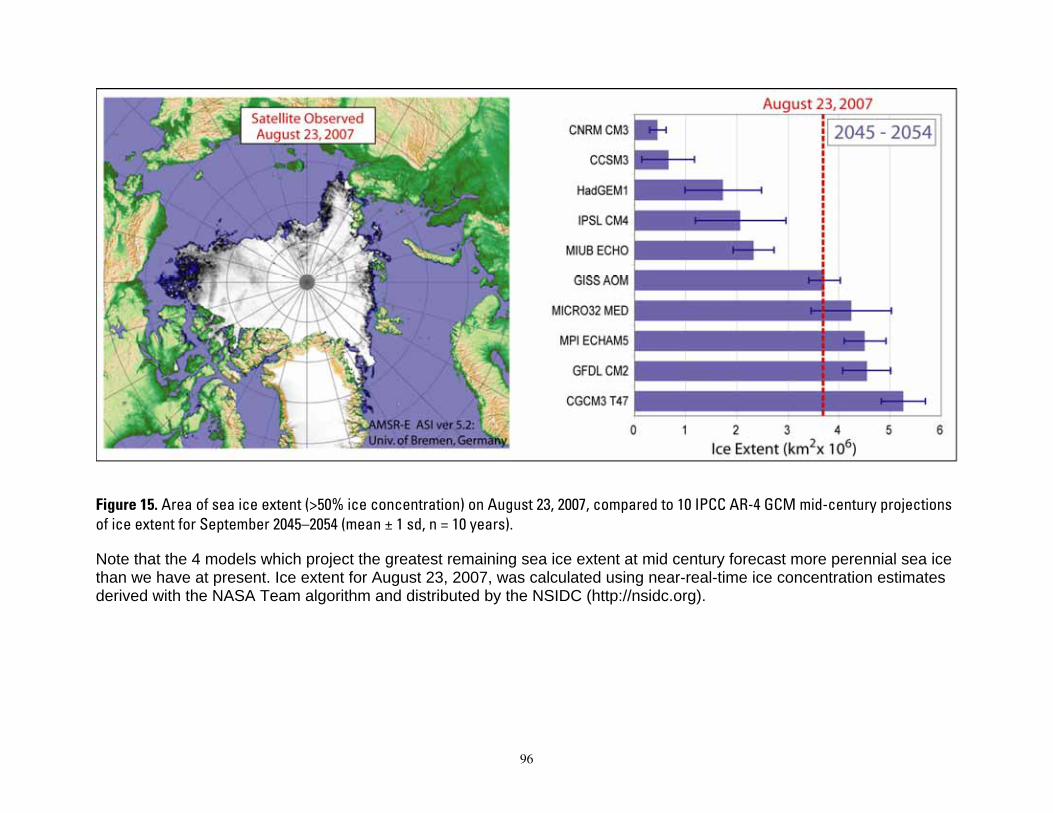
Figure 15. Area of sea ice extent (>50% ice concentration) on August 23, 2007, compared to 10 IPCC AR-4 GCM mid-century projections of ice extent for September 2045–2054 (mean ± 1 sd, n = 10 years).

Note that the 4 models which project the greatest remaining sea ice extent at mid century forecast more perennial sea ice than we have at present. Ice extent for August 23, 2007, was calculated using near-real-time ice concentration estimates derived with the NASA Team algorithm and distributed by the NSIDC (http://nsidc.org).

96

----------------------------------------------------------------------------

---- ------- --------------------------------

------------------------------------------------------------------------

--------------------------------------------------------------------

---- ------- --------------------------------

------------------------------------------------------------------------

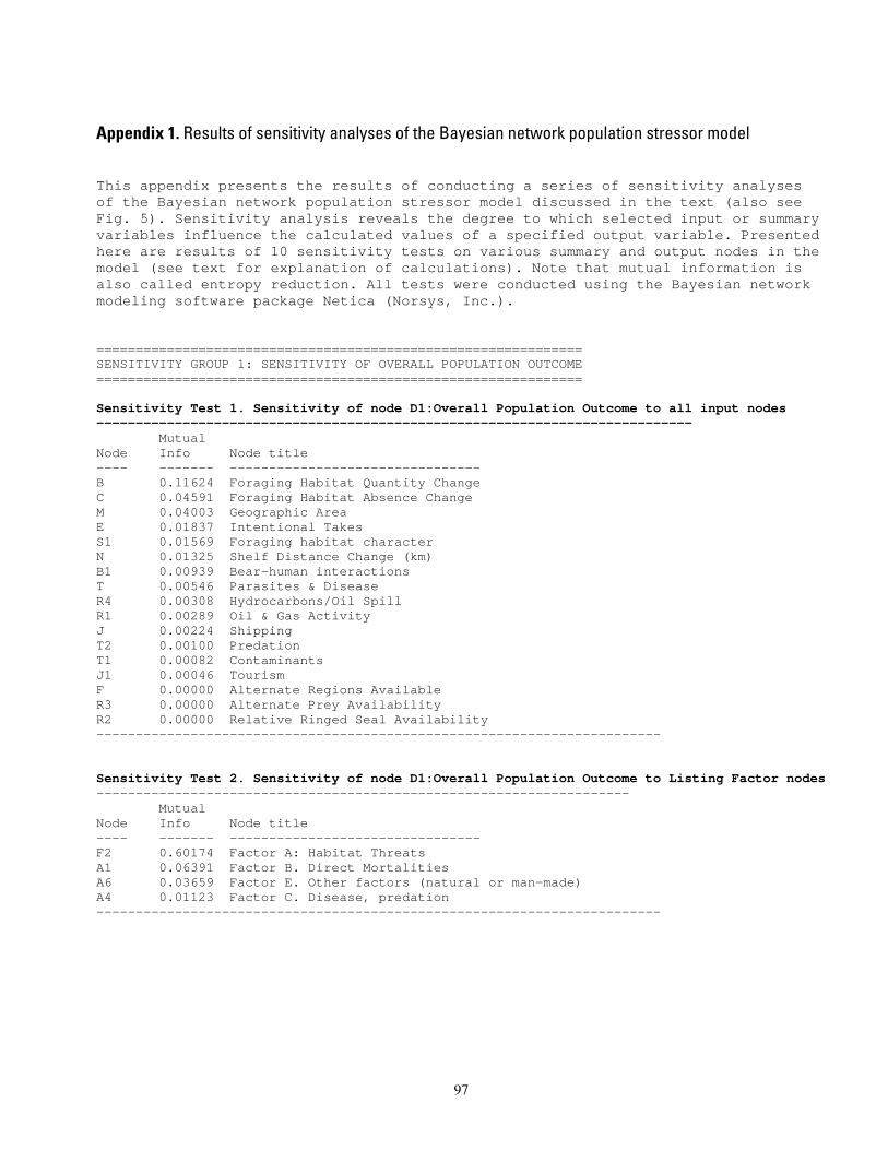
Appendix 1. Results of sensitivity analyses of the Bayesian network population stressor model

This appendix presents the results of conducting a series of sensitivity analyses of the Bayesian network population stressor model discussed in the text (also see Fig. 5). Sensitivity analysis reveals the degree to which selected input or summary variables influence the calculated values of a specified output variable. Presented here are results of 10 sensitivity tests on various summary and output nodes in the model (see text for explanation of calculations). Note that mutual information is also called entropy reduction. All tests were conducted using the Bayesian network modeling software package Netica (Norsys, Inc.).

============================================================== SENSITIVITY GROUP 1: SENSITIVITY OF OVERALL POPULATION OUTCOME ==============================================================

Sensitivity Test 1. Sensitivity of node D1:Overall Population Outcome to all input nodes

Mutual Node Info Node title

B 0.11624 Foraging Habitat Quantity Change C 0.04591 Foraging Habitat Absence Change M 0.04003 Geographic Area E 0.01837 Intentional Takes S1 0.01569 Foraging habitat character N 0.01325 Shelf Distance Change (km) B1 0.00939 Bear-human interactions T 0.00546 Parasites & Disease R4 0.00308 Hydrocarbons/Oil Spill R1 0.00289 Oil & Gas Activity J 0.00224 Shipping T2 0.00100 Predation T1 0.00082 Contaminants J1 0.00046 Tourism F 0.00000 Alternate Regions Available R3 0.00000 Alternate Prey Availability R2 0.00000 Relative Ringed Seal Availability

Sensitivity Test 2. Sensitivity of node D1:Overall Population Outcome to Listing Factor nodes

Mutual Node Info Node title

F2 0.60174 Factor A: Habitat Threats A1 0.06391 Factor B. Direct Mortalities A6 0.03659 Factor E. Other factors (natural or man-made) A4 0.01123 Factor C. Disease, predation

97

------------------------------------------------------------------------

------------------------------------------------------------------------

---- ------- --------------------------------

------------------------------------------------------------------------

---------------------------------------------------------------------------

-------------------------------------------------------------------------

---- ------- --------------------------------

-------------------------------------------------------------------------

-------------------------------------------------------------------------

---- ------- --------------------------------

-------------------------------------------------------------------------

-------------------------------------------------------------------------

---- ------- --------------------------------

-------------------------------------------------------------------------

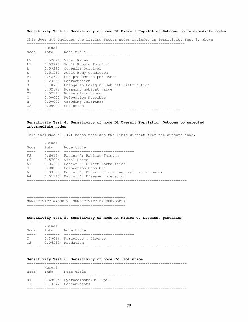
L

Sensitivity Test 3. Sensitivity of node D1:Overall Population Outcome to intermediate nodes

This does NOT includes the Listing Factor nodes included in Sensitivity Test 2, above.

Mutual Node Info Node title

L2 0.57024 Vital Rates L1 0.53323 Adult Female Survival

0.53295 Juvenile Survival K 0.51522 Adult Body Condition V1 0.42691 Cub production per event U 0.23368 Reproduction D 0.18791 Change in Foraging Habitat Distribution A 0.02592 Foraging habitat value C1 0.02114 Human disturbance G 0.00000 Relocation Possible H 0.00000 Crowding Tolerance C2 0.00000 Pollution

Sensitivity Test 4. Sensitivity of node D1:Overall Population Outcome to selected intermediate nodes

This includes all (6) nodes that are two links distant from the outcome node.

Mutual Node Info Node title

F2 0.60174 Factor A: Habitat Threats L2 0.57024 Vital Rates A1 0.06391 Factor B. Direct Mortalities G 0.00000 Relocation Possible A6 0.03659 Factor E. Other factors (natural or man-made) A4 0.01123 Factor C. Disease, predation

============================================= SENSITIVITY GROUP 2: SENSITIVITY OF SUBMODELS =============================================

Sensitivity Test 5. Sensitivity of node A4:Factor C. Disease, predation

Mutual Node Info Node title

T 0.39016 Parasites & Disease T2 0.06593 Predation

Sensitivity Test 6. Sensitivity of node C2: Pollution

Mutual Node Info Node title

R4 0.69005 Hydrocarbons/Oil Spill T1 0.13542 Contaminants

98

-------------------------------------------------------------------------

-------------------------------------------------------------------------

-------------------------------------------------------------------------

---- ------- --------------------------------

-------------------------------------------------------------------------

-------------------------------------------------------------------------

---- ------- --------------------------------

-------------------------------------------------------------------------

-------------------------------------------------------------------------

---- ------- --------------------------------

-------------------------------------------------------------------------

Sensitivity Test 7. Sensitivity of node C1:Human disturbance

Mutual Node Info Node title ---- ------- --------------------------------B1 0.45796 Bear-human interactions R1 0.12450 Oil & Gas Activity J 0.08941 Shipping J1 0.01729 Tourism

Sensitivity Test 8. Sensitivity of node A:Foraging habitat value

Mutual Node Info Node title

S1 0.63429 Foraging habitat character F 0.00000 Alternate Regions Available R3 0.00000 Alternate Prey Availability R2 0.00000 Relative Ringed Seal Availability

Sensitivity Test 9. Sensitivity of node D:Change in Foraging Habitat Distribution

Mutual Node Info Node title

M 0.33239 Geographic Area C 0.32674 Foraging Habitat Absence Change N 0.06131 Shelf Distance Change (km)

Sensitivity Test 10. Sensitivity of node L2:Vital Rates

Mutual Node Info Node title

L1 1.09792 Adult Female Survival L 1.09537 Juvenile Survival F2 0.99215 Factor A: Habitat Threats K 0.97559 Adult Body Condition V1 0.69213 Cub production per event U 0.36497 Reproduction M 0.04728 Geographic Area N 0.01955 Shelf Distance Change (km)

99

Appendix 2. Documentation of the Bayesian network polar bear population stressor model

This appendix documents the structure of the Bayesian network (BN) population stressor model. We used the BN modeling shell Netica® (Norsys, Inc.) to create a model that represents potential influences on distribution response, numerical response, and overall population response of polar bears under multiple stressors, which include anthropogenic stressors, natural disturbances, and other key environmental correlates to polar bear population amount and distribution.

The BN population stressor model was created to represent the knowledge and judgment of one polar bear biologist (S. Amstrup) with guidance from an ecologist modeler (B. Marcot). See the text for a brief explanations of Bayesian modeling and statistics. The general underlying influence diagram for the BN model is shown in Figure 4, and the full model is in Figure 5. A BN model consists of a series of variables represented as “nodes” (boxes in Fig. 5) that interact through links (arrows in Fig. 5). Nodes that have no incoming arrows are “input nodes” (the yellow boxes in Fig. 5, e.g., node T Parasites & Disease). Nodes with both incoming and outgoing arrows are summary nodes (or latent variables, e.g., node L2 Vital Rates). In our model, we also specified four of the summary nodes as listing factors used by USDI Fish and Wildlife Service (S. Morey, pers. comm.). Nodes with incoming arrows but no outgoing arrows are outcome nodes (node D1 Overall Population Outcome).

Each node in this model consists of a short node name (e.g., node D1), a longer node title (e.g., Overall Population Outcome), a set of states (e.g, larger, same as now, smaller, rare, and extinct), and an underlying probability table. The probability tables consist of unconditional (or prior) probabilities in the input nodes, or conditional probabilities in all other nodes, the latter representing probabilities of each state as a function of (conditional upon) the states of all nodes that directly influence it.

The following table presents a complete list of all nodes in the model with their short code letter names, their fuller titles, a description, their states, and the group (Node Set, in Netica parlance) to which it belongs (input nodes, output node, summary node, or summary listing factor node).

100

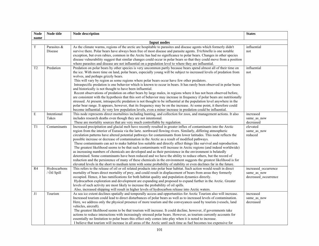
Node name

Node title Node description States

Input nodes T Parasites &

Disease As the climate warms, regions of the arctic are hospitable to parasites and disease agents which formerly didn't survive there. Polar bears have always been free of most disease and parasite agents. Trichinella is one notable exception, but even rabies, common in the Arctic has had no significance to polar bears. Changes in other species disease vulnerability suggest that similar changes could occur in polar bears so that they could move from a position where parasites and disease are not influential on a population level to where they are influential.

influential not

T2 Predation Predation on polar bears by other species is very uncommon partly because bears spend almost all of their time on the ice. With more time on land, polar bears, especially young will be subject to increased levels of predation from wolves, and perhaps grizzly bears. This will vary by region as some regions where polar bears occur have few other predators. Intraspecific predation is one behavior which is known to occur in bears. It has rarely been observed in polar bears and historically is not thought to have been influential. Recent observations of predation on other bears by large males, in regions where it has not been observed before, are consistent with the hypothesis that this sort of behavior may increase in frequency if polar bears are nutritionally stressed. At present, intraspecific predation is not thought to be influential at the population level anywhere in the polar bear range. It appears, however, that its frequency may be on the increase. At some point, it therefore could become influential. At very low population levels, even a miner increase in predation could be influential.

influential not

E Intentional Takes

This node represents direct mortalities including hunting, and collection for zoos, and management actions. It also includes research deaths even though they are not intentional. These are mortality sources that are very much controllable by regulation.

increased same_as_now decreased

T1 Contaminants Increased precipitation and glacial melt have recently resulted in greater influx of contaminants into the Arctic region from the interior of Eurasia via the larte. northward flowing rivers. Similarly, differing atmospheric circulation patterns have altered potential pathways for contaminants from lower latitudes. This node reflects the possible increase or decrease of contamination in the Arctic as a result of modified pathways. These contaminants can act to make habitat less suitable and directly affect things like survival and reproduction. The greatest likelihood seems to be that such contaminants will increase in Arctic regions (and indeed worldwide) as increasing numbers of chemicals are developed and as their persistence in the environment is belatedly determined. Some contaminants have been reduced and we have the ability to reduce others, but the record of reduction and the persistence of many of these chemicals in the environment suggests the greatest likelihood is for elevated levels in the short to medium term with some probability of stability or even declines far in the future.

elevated same_as_now reduced

R4 Hydrocarbons / Oil Spill

This refers to the release of oil or oil related products into polar bear habitat. Such action would result in direct mortality of bears direct mortality of prey, and could result in displacement of bears from areas they formerly occupied. Hence, it has ramifications for both habitat quality and population dynamics directly. Hydrocarbon exploration and development are expanding and proposed to expand further in the Arctic. Greater levels of such activity are most likely to increase the probability of oil spills. Also, increased shipping will result in higher levels of hydrocarbon release into Arctic waters.

increased_occurrence same_as_now decreased_occurrence

J1 Tourism As sea ice extent declines spatially and temporally access and opportunities for Arctic Tourism also will increase. Increased tourism could lead to direct disturbances of polar bears as well as to increased levels of contamination. Here, we address only the physical presence of more tourism and the conveyances used by tourists (vessels, land vehicles, aircraft). The greatest likelihood seems to be that tourism will increase. It could decline, however, if governments take actions to reduce interactions with increasingly stressed polar bears. However, as tourism currently accounts for essentially no limitation to polar bears this effect only comes into play when it is noted to increase. I believe that tourism will increase in all areas of the Arctic until such time as fuel becomes too expensive for

increased same_as_now decreased

101

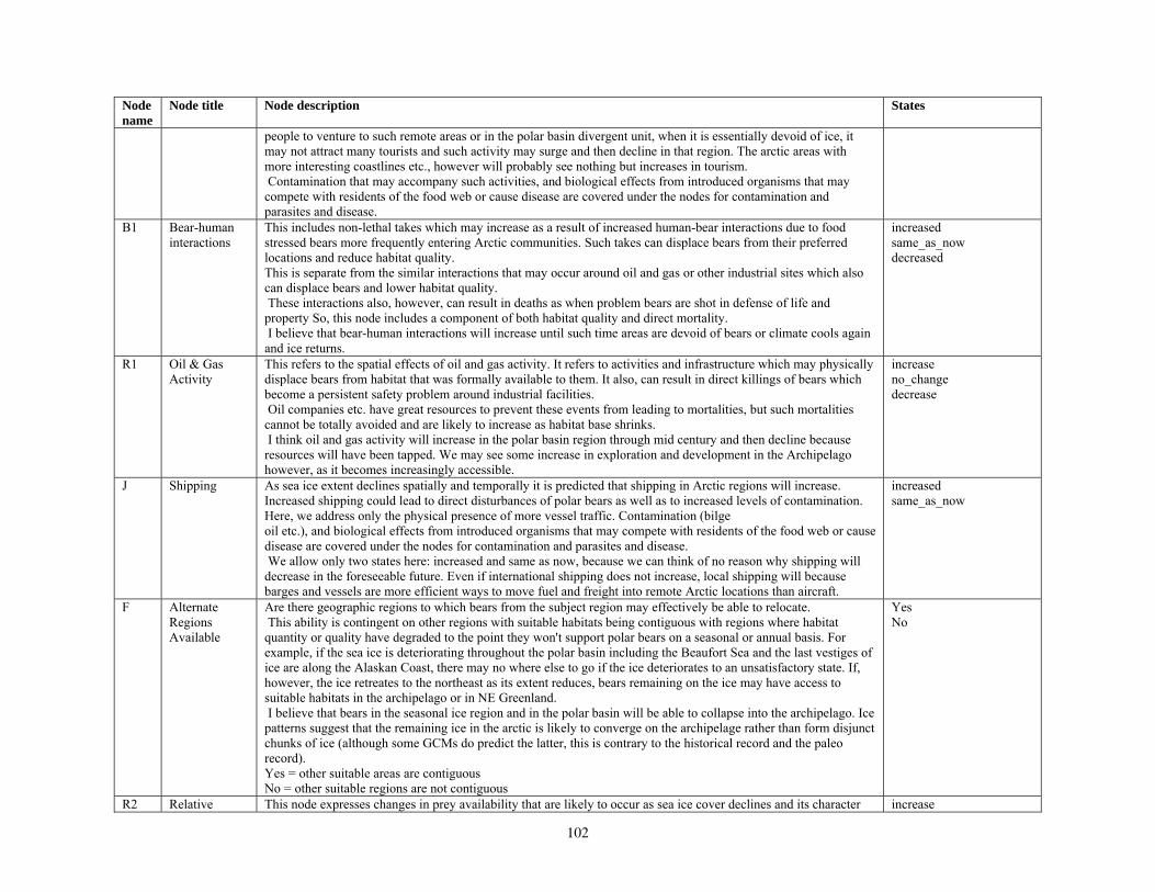
Node name

Node title Node description States

people to venture to such remote areas or in the polar basin divergent unit, when it is essentially devoid of ice, it may not attract many tourists and such activity may surge and then decline in that region. The arctic areas with more interesting coastlines etc., however will probably see nothing but increases in tourism. Contamination that may accompany such activities, and biological effects from introduced organisms that may compete with residents of the food web or cause disease are covered under the nodes for contamination and parasites and disease.

B1 Bear-human interactions

This includes non-lethal takes which may increase as a result of increased human-bear interactions due to food stressed bears more frequently entering Arctic communities. Such takes can displace bears from their preferred locations and reduce habitat quality. This is separate from the similar interactions that may occur around oil and gas or other industrial sites which also can displace bears and lower habitat quality. These interactions also, however, can result in deaths as when problem bears are shot in defense of life and property So, this node includes a component of both habitat quality and direct mortality. I believe that bear-human interactions will increase until such time areas are devoid of bears or climate cools again and ice returns.

increased same_as_now decreased

R1 Oil & Gas Activity

This refers to the spatial effects of oil and gas activity. It refers to activities and infrastructure which may physically displace bears from habitat that was formally available to them. It also, can result in direct killings of bears which become a persistent safety problem around industrial facilities. Oil companies etc. have great resources to prevent these events from leading to mortalities, but such mortalities cannot be totally avoided and are likely to increase as habitat base shrinks. I think oil and gas activity will increase in the polar basin region through mid century and then decline because resources will have been tapped. We may see some increase in exploration and development in the Archipelago however, as it becomes increasingly accessible.

increase no_change decrease

J Shipping As sea ice extent declines spatially and temporally it is predicted that shipping in Arctic regions will increase. Increased shipping could lead to direct disturbances of polar bears as well as to increased levels of contamination. Here, we address only the physical presence of more vessel traffic. Contamination (bilge oil etc.), and biological effects from introduced organisms that may compete with residents of the food web or cause disease are covered under the nodes for contamination and parasites and disease. We allow only two states here: increased and same as now, because we can think of no reason why shipping will decrease in the foreseeable future. Even if international shipping does not increase, local shipping will because barges and vessels are more efficient ways to move fuel and freight into remote Arctic locations than aircraft.

increased same_as_now

F Alternate Regions Available

Are there geographic regions to which bears from the subject region may effectively be able to relocate. This ability is contingent on other regions with suitable habitats being contiguous with regions where habitat

quantity or quality have degraded to the point they won't support polar bears on a seasonal or annual basis. For example, if the sea ice is deteriorating throughout the polar basin including the Beaufort Sea and the last vestiges of ice are along the Alaskan Coast, there may no where else to go if the ice deteriorates to an unsatisfactory state. If, however, the ice retreates to the northeast as its extent reduces, bears remaining on the ice may have access to suitable habitats in the archipelago or in NE Greenland. I believe that bears in the seasonal ice region and in the polar basin will be able to collapse into the archipelago. Ice patterns suggest that the remaining ice in the arctic is likely to converge on the archipelage rather than form disjunct chunks of ice (although some GCMs do predict the latter, this is contrary to the historical record and the paleo record). Yes = other suitable areas are contiguous No = other suitable regions are not contiguous

Yes No

R2 Relative This node expresses changes in prey availability that are likely to occur as sea ice cover declines and its character increase

102

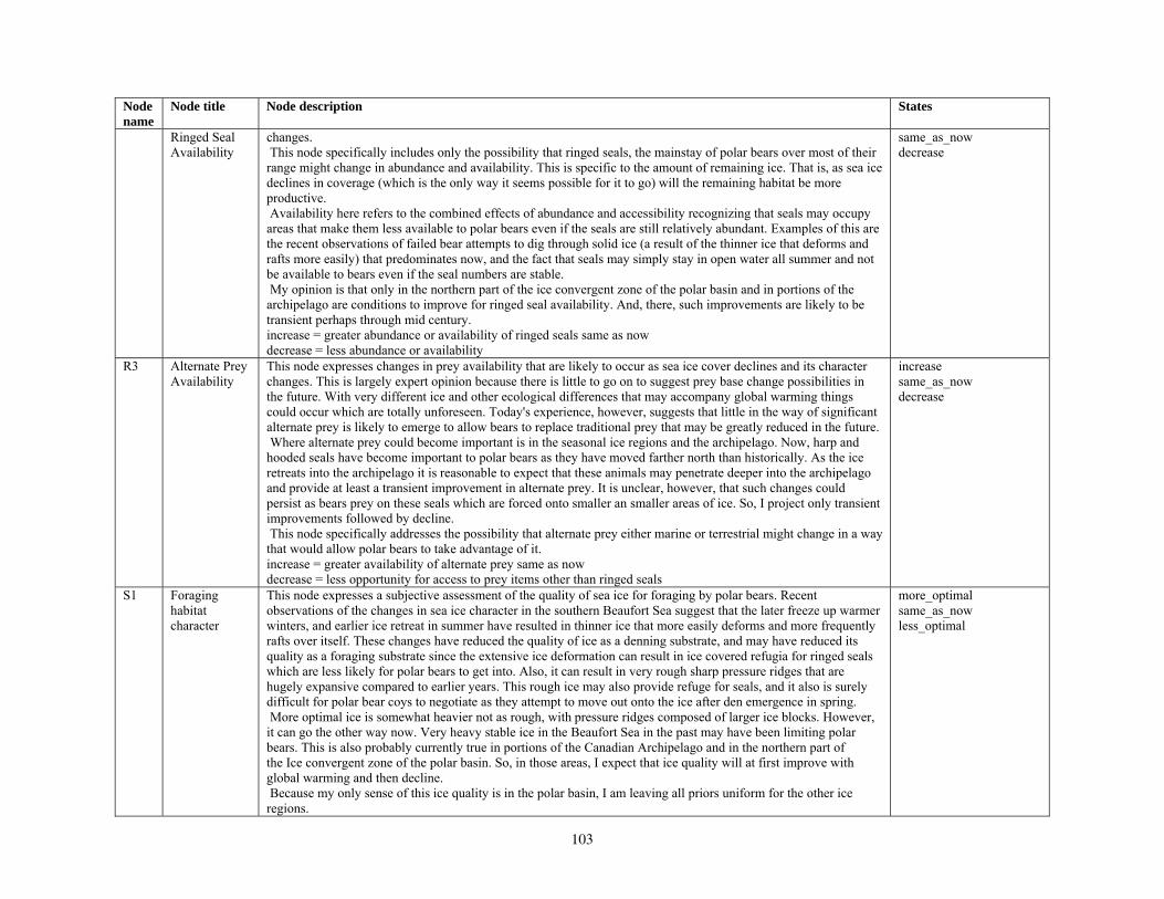
Node name

Node title Node description States

Ringed Seal changes. same_as_now Availability This node specifically includes only the possibility that ringed seals, the mainstay of polar bears over most of their

range might change in abundance and availability. This is specific to the amount of remaining ice. That is, as sea ice declines in coverage (which is the only way it seems possible for it to go) will the remaining habitat be more productive. Availability here refers to the combined effects of abundance and accessibility recognizing that seals may occupy areas that make them less available to polar bears even if the seals are still relatively abundant. Examples of this are the recent observations of failed bear attempts to dig through solid ice (a result of the thinner ice that deforms and rafts more easily) that predominates now, and the fact that seals may simply stay in open water all summer and not be available to bears even if the seal numbers are stable. My opinion is that only in the northern part of the ice convergent zone of the polar basin and in portions of the archipelago are conditions to improve for ringed seal availability. And, there, such improvements are likely to be transient perhaps through mid century. increase = greater abundance or availability of ringed seals same as now decrease = less abundance or availability

decrease

R3 Alternate Prey Availability

This node expresses changes in prey availability that are likely to occur as sea ice cover declines and its character changes. This is largely expert opinion because there is little to go on to suggest prey base change possibilities in the future. With very different ice and other ecological differences that may accompany global warming things could occur which are totally unforeseen. Today's experience, however, suggests that little in the way of significant alternate prey is likely to emerge to allow bears to replace traditional prey that may be greatly reduced in the future. Where alternate prey could become important is in the seasonal ice regions and the archipelago. Now, harp and hooded seals have become important to polar bears as they have moved farther north than historically. As the ice retreats into the archipelago it is reasonable to expect that these animals may penetrate deeper into the archipelago and provide at least a transient improvement in alternate prey. It is unclear, however, that such changes could persist as bears prey on these seals which are forced onto smaller an smaller areas of ice. So, I project only transient improvements followed by decline. This node specifically addresses the possibility that alternate prey either marine or terrestrial might change in a way that would allow polar bears to take advantage of it. increase = greater availability of alternate prey same as now decrease = less opportunity for access to prey items other than ringed seals

increase same_as_now decrease

S1 Foraging habitat character

This node expresses a subjective assessment of the quality of sea ice for foraging by polar bears. Recent observations of the changes in sea ice character in the southern Beaufort Sea suggest that the later freeze up warmer winters, and earlier ice retreat in summer have resulted in thinner ice that more easily deforms and more frequently rafts over itself. These changes have reduced the quality of ice as a denning substrate, and may have reduced its quality as a foraging substrate since the extensive ice deformation can result in ice covered refugia for ringed seals which are less likely for polar bears to get into. Also, it can result in very rough sharp pressure ridges that are hugely expansive compared to earlier years. This rough ice may also provide refuge for seals, and it also is surely difficult for polar bear coys to negotiate as they attempt to move out onto the ice after den emergence in spring. More optimal ice is somewhat heavier not as rough, with pressure ridges composed of larger ice blocks. However, it can go the other way now. Very heavy stable ice in the Beaufort Sea in the past may have been limiting polar bears. This is also probably currently true in portions of the Canadian Archipelago and in the northern part of the Ice convergent zone of the polar basin. So, in those areas, I expect that ice quality will at first improve with global warming and then decline. Because my only sense of this ice quality is in the polar basin, I am leaving all priors uniform for the other ice regions.

more_optimal same_as_now less_optimal

103

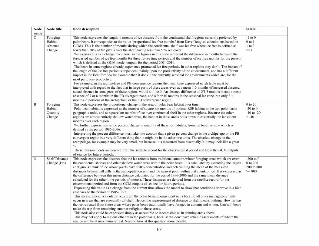
Node name

Node title Node description States

C Foraging This node expresses the length in months of ice absence from the continental shelf regions currently preferred by -1 to 0 Habitat polar bears. It correspondes to the value "proportional ice free months" from Dave Douglas' calculations based on 0 to 1 Absence GCMs. This is the number of months during which the continental shelf was ice free where ice free is defined as 1 to 3 Change fewer than 50% of the pixels over the shelf having less than 50% ice cover.

We express this as a change from now. so the figures in this node represent the difference in months between the forecasted number of ice free months for three future time periods and the number of ice free months for the present which is defined as the GCM model outputs for the period 2001-2010. The bears in some regions already experience protracted ice free periods. In other regions they don’t. The impact of the length of the ice free period is dependent mainly upon the productivity of the environment, and has a different impact in the Beaufort Sea for example than it does in the currently seasonal ice environments which are, for the most part, very productive. For example, in the archipelago and PB convergence regions the mean time expressed in teh table must be interpreted with regard to the fact that in large parts of these areas even at a mean 1-3 months of increased absence, actual absence in some parts of these regions would still be 0. An absence difference of GT 3 months means a mean absence of 7 or 8 months in the PB divergent zone, and 8 9 or 10 months in the seasonal ice zone, but only 3 + months in portions of the archipelago or the PB convergence region.

>=3

B Foraging This node expresses the proportional change in the area of polar bear habitat over time. 0 to 20 Habitat Polar bear habitat is expressed as the number of square km months of optimal RSF habitat in the two polar basin -20 to 0 Quantity geographic units, and as square km months of ice over continental shelf in the other regions. Because the other -40 to -20 Change regions are almost entirely shallow water areas, the habitat in those areas boils down to essentially the ice extent

months over each region. We further express this as the percent change in quantity of these ice habitats, from the baseline now which is defined as the period 1996-2006. Interpreting the percent difference must take into account that a given percent change in the archipelago or the PB convergent region is a very different thing than it might be in the other two units. The absolute change in the archipelago, for example may be very small, but because it is measured from essentially 0, it may look like a great % . These measurements are derived from the satellite record for the observational period and from the GCM outputs of sea ice for future periods.

< -40

N Shelf Distance This node expresses the distance that the ice retreats from traditional autumn/winter foraging areas which are over -200 to 0 Change (km) the continental shelves and other shallow water areas within the polar basin. It is calculated by extracting the largest 0 to 200

contiguous chunk of ice whose pixels have >50% concentration and determining the mean of the measured 200 to 800 distances between all cells in the subpopulation unit and the nearest point within that chunk of ice. It is expressed as the difference between this mean distance calculated for the period 1996-2006 and the same mean distance calculated for the other time periods of interest. These distances are derived from the satellite record for the observational period and from the GCM outputs of sea ice for future periods. Expressing this value as a change from the current time allows the model to show that conditions improve in a hind cast back to the period of 1985-1995. This measurement is available only from the polar basin management units because all other management units occur in areas that are essentially all shelf. Hence, the measurement of distance to shelf means nothing. How far has the ice retreated from shore areas where polar bears traditionally have foraged in autumn and winter. Can/will bears make the trip from remaining summer refugia to these areas. This node also could be expressed simply as accessible or inaccessible as in denning areas above. This may not apply to regions other than the polar basin, because we don't have reliable assessments of where the sea ice will be at maximum retreat. Need to look at this question more closely.

>= 800

104

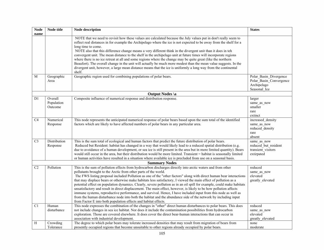
Node name

Node title Node description States

NOTE that we need to revisit how these values are calculated because the July values put in don't really seem to reflect real distances in for example the Archipelago where the ice is not expected to be away from the shelf for a long time to come. NOTE also that this difference change means a very different think in the divergent unit than it does in teh convergent unit. The mean distance to the shelf in the archipelago unit at future times will incorporate regions where there is no ice retreat at all and some regions where the change may be quite great (like the northern Beaufort). The overall change in the unit will actually be much more modest than the mean value suggests. In the divergent unit, however, a large mean distance means that the ice is uniformly a long way from the continental shelf.

M Geographic Area

Geographic region used for combining populations of polar bears. Polar_Basin_Divergence Polar_Basin_Convergence Archipelago Seasonal_Ice

Output Nodes \a D1 Overall

Population Outcome

Composite influence of numerical response and distribution response. larger same_as_now smaller rare extinct

C4 Numerical Response

This node represents the anticipated numerical response of polar bears based upon the sum total of the identified factors which are likely to have affected numbers of polar bears in any particular area.

increased_density same_as_now reduced_density rare absent

C3 Distribution Response

This is the sum total of ecological and human factors that predict the future distribution of polar bears. Reduced but Resident: habitat has changed in a way that would likely lead to a reduced spatial distribution (e.g. due to avoidance of a human development, or sea ice is still present in the area but in more limited quantity). Bears would still occur in the area, but their distribution would be more limited. Transient = habitat is seasonally limited or human activities have resulted in a situation where available ice is precluded from use on a seasonal basis.

same_as_now reduced_but_resident transient_visitors extirpated

Summary Nodes C2 Pollution This is the sum of pollution effects from hydrocarbon discharges directly into arctic waters and from other

pollutants brought to the Arctic from other parts of the world. The FWS listing proposal included Pollution as one of the "other factors" along with direct human bear interactions that may displace bears or otherwise make habitats less satisfactory, I viewed the main effect of pollution as a potential effect on population dynamics. Clearly, severe pollution as in an oil spill for example, could make habitats unsatisfactory and result in direct displacement. The main effect, however, is likely to be how pollution affects immune systems, reproductive performance, and survival. Hence, I have included input from this node as well as from the human disturbance node into both the habitat and the abundance side of the network by including input from Factor E into both population effects and habitat effects.

reduced same_as_now elevated greatly_elevated

C1 Human disturbance

This node expresses the combination of the changes in "other" direct human disturbances to polar bears. This does not include changes in sea ice habitat. Nor does it include the contamination possibilities from hydrocarbon exploration. Those are covered elsewhere. It does cover the direct bear-human interactions that can occur in association with industrial development.

reduced same_as_now elevated greatly_elevated

H Crowding Tolerance

The degree to which polar bears may tolerate increased densities that may result from migration of bears from presently occupied regions that become unsuitable to other regions already occupied by polar bears.

none moderate

105

Node name

Node title Node description States

In essence, this is the tolerance of bears to live in more crowded conditions than those at which they presently live. And, it is a function of food availability I believe that bears have a reasonable tolerance of crowding if food is abundant or if they are in good condition while waiting for sea ice to return etc. Examples of these situations include 1) portions of the high arctic like near resolute, where bear densities on the sea ice in spring are apparently much higher than they are in most of the polar basin, and 2) the high densities at which polar bears occur on land in Hudson Bay in summer when they are loafing and waiting for the sea ice to return. I assumed that crowding tolerance has little or no effect on outcome likelihoods until habitat quantity was reduced substantially requiring bears from one area to either perish or find some place else to go on at least a seasonal basis. Thereafter, if relocations of members of some subpopulations meant invading the areas occupied by other bears crowding tolerance entered an assessment of whether or not relocation was a practical solution.

high

G Relocation Possible

Is it likely that polar bears displaced from one region could either seasonally or permanently relocate to another region in order to persist. This is a function of foraging effects (e.g. prey availability) in the alternative area (here I am specifically focusing on prey availability in the alternative area rather than the area from which the bears may have been displaced) crowding tolerance, and contiguity of habitats.

Yes No

A Foraging habitat value

This node expresses the sum total of things which may work to alter the quality of habitats available to polar bears in the future. The idea here is that sea ice is retreating spatially and temporally, but is the ice that remains of comparable, better or worse quality as polar bear habitat. Our RSF values are projected into the future with the assumption that a piece of ice in 2090 that looks the same as piece of ice in 1985 has the same value to a polar bear. Perhaps because of responses we cannot foresee, it may be better seal habitat, or it may be habitat for an alternate prey. Conversely, it may be worse because of atmospheric and oceanic processes (e.g. the epontic community is less vibrant due to thinner ice which is not around for as long each year). Or it may be worse habitat because of oil and gas development, tourism, shipping etc.

better same_as_now worse

D Change in Foraging Habitat Distribution

This node expresses the combination of the quantitative ways the retreat of sea ice may affect use of continental shelf habitats. Our analyses indicate, in addition to reductions of total ice (and RSF Optimum ice) extent (expressed under habitat quantity), we will see seasonal retreats of the sea ice away from coastal areas now preferred by polar bears, and these retreats are projected to progressively become longer. These changes will affect polar bears by reducing the total availability of ice substrate for bears. They also will make ice unavailable for extended periods in many regions bears now occur year round. This will result in the opportunity for seasonal occupancy but not year-round occupancy as they have had in the past. Note that in the PB Convergent unit because it includes the NB and QE and EG each of which has different starting points, the values in the CPT express kind of an average. Similarly, in the Seasonal region, there is a huge difference between HBay and Foxe Basin or BB. so, again the CPT values are a sort of an average, trying to reflect these differences. Ultimately, we need to subdivide these regions a bit more to really reflect what is going on. Also note that the "same as now" category doesn't really work very well for the seasonal ice environment where now is seasonal. The only way to go from here is to better than now or to sporadic. Having a step between now and sporadic is not useful. In fact, all of these categories need to be changed.

improved_availability same_as_now reduced_avail Gr_reduced_avail Unavailable

L2 Vital Rates This expresses the combined effect of changes in survival of adult females and of young and reproductive patterns. The probabilities assigned each of the states reflects the relative importance to polar bear population dynamics of each of these vital rates to the growth of the population. This node does not reflect human influences on population growth such as hunting, or mortalities resulting from bear-human interactions. Those things, along with effects of parasites, contaminants, etc. are brought in as modifiers at the level of the next node.

improve same_as_now decline

106

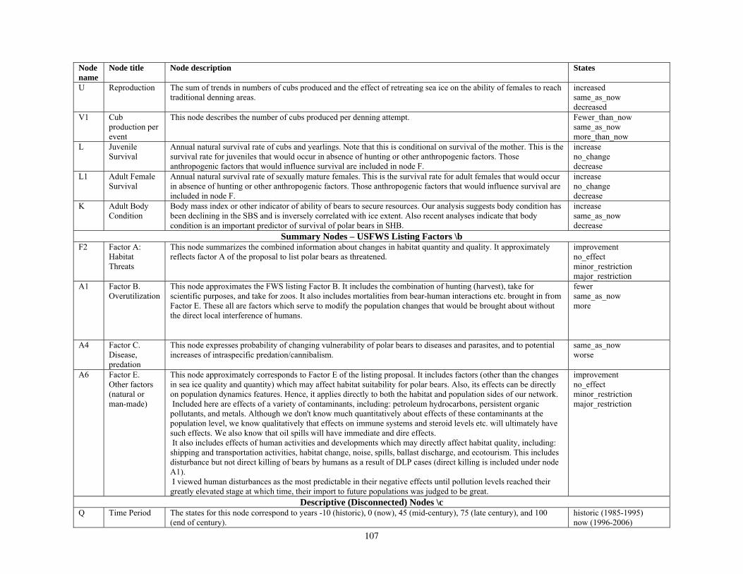
Node name

Node title Node description States

U Reproduction The sum of trends in numbers of cubs produced and the effect of retreating sea ice on the ability of females to reach traditional denning areas.

increased same_as_now decreased

V1 Cub production per event

This node describes the number of cubs produced per denning attempt. Fewer_than_now same_as_now more_than_now

L Juvenile Survival

Annual natural survival rate of cubs and yearlings. Note that this is conditional on survival of the mother. This is the survival rate for juveniles that would occur in absence of hunting or other anthropogenic factors. Those anthropogenic factors that would influence survival are included in node F.

increase no_change decrease

L1 Adult Female Survival

Annual natural survival rate of sexually mature females. This is the survival rate for adult females that would occur in absence of hunting or other anthropogenic factors. Those anthropogenic factors that would influence survival are included in node F.

increase no_change decrease

K Adult Body Condition

Body mass index or other indicator of ability of bears to secure resources. Our analysis suggests body condition has been declining in the SBS and is inversely correlated with ice extent. Also recent analyses indicate that body condition is an important predictor of survival of polar bears in SHB.

increase same_as_now decrease

Summary Nodes – USFWS Listing Factors \b F2 Factor A:

Habitat Threats

This node summarizes the combined information about changes in habitat quantity and quality. It approximately reflects factor A of the proposal to list polar bears as threatened.

improvement no_effect minor_restriction major_restriction

A1 Factor B. Overutilization

This node approximates the FWS listing Factor B. It includes the combination of hunting (harvest), take for scientific purposes, and take for zoos. It also includes mortalities from bear-human interactions etc. brought in from Factor E. These all are factors which serve to modify the population changes that would be brought about without the direct local interference of humans.

fewer same_as_now more

A4 Factor C. Disease, predation

This node expresses probability of changing vulnerability of polar bears to diseases and parasites, and to potential increases of intraspecific predation/cannibalism.

same_as_now worse

A6 Factor E. Other factors (natural or man-made)

This node approximately corresponds to Factor E of the listing proposal. It includes factors (other than the changes in sea ice quality and quantity) which may affect habitat suitability for polar bears. Also, its effects can be directly on population dynamics features. Hence, it applies directly to both the habitat and population sides of our network. Included here are effects of a variety of contaminants, including: petroleum hydrocarbons, persistent organic pollutants, and metals. Although we don't know much quantitatively about effects of these contaminants at the population level, we know qualitatively that effects on immune systems and steroid levels etc. will ultimately have such effects. We also know that oil spills will have immediate and dire effects. It also includes effects of human activities and developments which may directly affect habitat quality, including: shipping and transportation activities, habitat change, noise, spills, ballast discharge, and ecotourism. This includes disturbance but not direct killing of bears by humans as a result of DLP cases (direct killing is included under node A1). I viewed human disturbances as the most predictable in their negative effects until pollution levels reached their greatly elevated stage at which time, their import to future populations was judged to be great.

improvement no_effect minor_restriction major_restriction

Descriptive (Disconnected) Nodes \c Q Time Period The states for this node correspond to years -10 (historic), 0 (now), 45 (mid-century), 75 (late century), and 100

(end of century). historic (1985-1995) now (1996-2006)

107

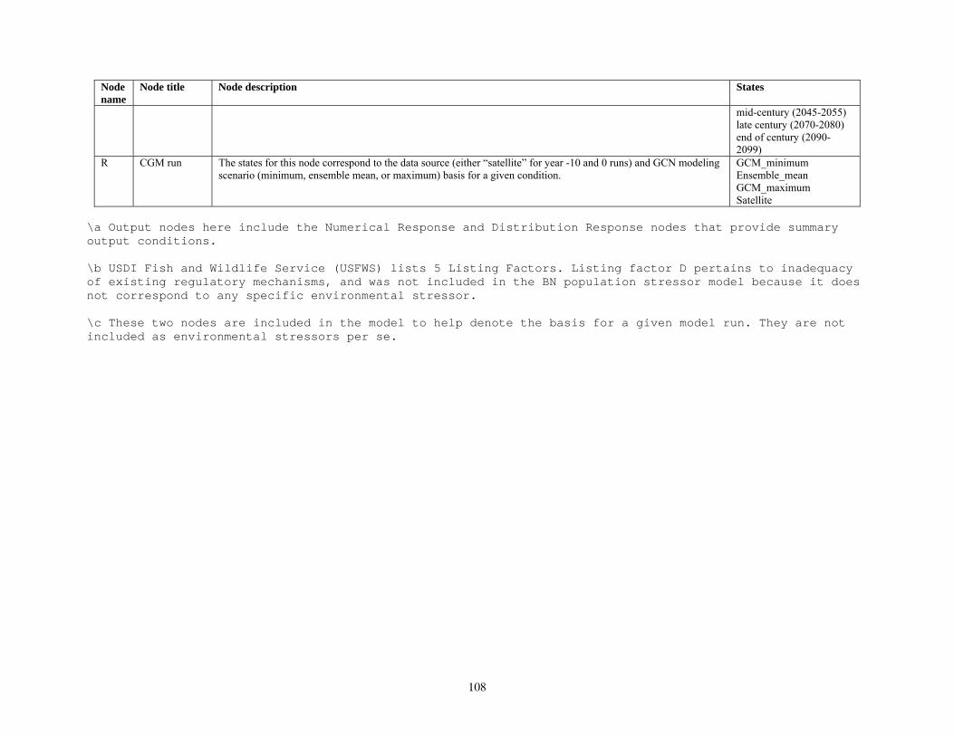
Node name

Node title Node description States

mid-century (2045-2055) late century (2070-2080) end of century (2090­2099)

R CGM run The states for this node correspond to the data source (either “satellite” for year -10 and 0 runs) and GCN modeling scenario (minimum, ensemble mean, or maximum) basis for a given condition.

GCM_minimum Ensemble_mean GCM_maximum Satellite

\a Output nodes here include the Numerical Response and Distribution Response nodes that provide summary

output conditions.

\b USDI Fish and Wildlife Service (USFWS) lists 5 Listing Factors. Listing factor D pertains to inadequacy

of existing regulatory mechanisms, and was not included in the BN population stressor model because it does

not correspond to any specific environmental stressor.

\c These two nodes are included in the model to help denote the basis for a given model run. They are not

included as environmental stressors per se.

108

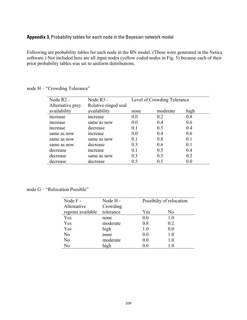
Appendix 3. Probability tables for each node in the Bayesian network model

Following are probability tables for each node in the BN model. (These were generated in the Netica software.) Not included here are all input nodes (yellow coded nodes in Fig. 5) because each of their prior probability tables was set to uniform distributions.

node H – “Crowding Tolerance”

Node R2 - Node R3 - Level of Crowding Tolerance Alternative prey Relative ringed seal availability availability none moderate high increase increase 0.0 0.2 0.8 increase same as now 0.0 0.4 0.6 increase decrease 0.1 0.5 0.4 same as now increase 0.0 0.4 0.6 same as now same as now 0.1 0.8 0.1 same as now decrease 0.3 0.6 0.1 decrease increase 0.1 0.5 0.4 decrease same as now 0.3 0.5 0.2 decrease decrease 0.5 0.5 0.0

node G – “Relocation Possible”

Node F - Node H - Possibilty of relocation Alternative Crowding regions available tolerance Yes No Yes none 0.0 1.0 Yes moderate 0.8 0.2 Yes high 1.0 0.0 No none 0.0 1.0 No moderate 0.0 1.0 No high 0.0 1.0

109

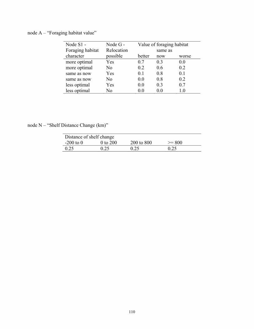
node A – “Foraging habitat value”

Node S1 - Node G - Value of foraging habitat Foraging habitat Relocation same as character possible better now worse more optimal Yes 0.7 0.3 0.0 more optimal No 0.2 0.6 0.2 same as now Yes 0.1 0.8 0.1 same as now No 0.0 0.8 0.2 less optimal Yes 0.0 0.3 0.7 less optimal No 0.0 0.0 1.0

node N – “Shelf Distance Change (km)”

Distance of shelf change -200 to 0 0 to 200 200 to 800 >= 800 0.25 0.25 0.25 0.25

110

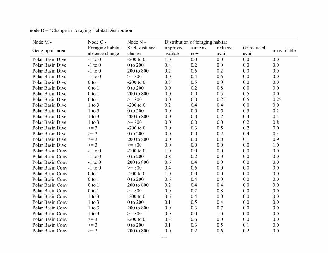
node D – “Change in Foraging Habitat Distribution”

Node M - Node C - Node N - Distribution of foraging habitat

Geographic area Foraging habitat absence change

Shelf distance change

improved availab

same as now

reduced avail

Gr reduced avail unavailable

Polar Basin Dive -1 to 0 -200 to 0 1.0 0.0 0.0 0.0 0.0 Polar Basin Dive -1 to 0 0 to 200 0.8 0.2 0.0 0.0 0.0 Polar Basin Dive -1 to 0 200 to 800 0.2 0.6 0.2 0.0 0.0 Polar Basin Dive -1 to 0 >= 800 0.0 0.4 0.6 0.0 0.0 Polar Basin Dive 0 to 1 -200 to 0 0.5 0.5 0.0 0.0 0.0 Polar Basin Dive 0 to 1 0 to 200 0.0 0.2 0.8 0.0 0.0 Polar Basin Dive 0 to 1 200 to 800 0.0 0.0 0.5 0.5 0.0 Polar Basin Dive 0 to 1 >= 800 0.0 0.0 0.25 0.5 0.25 Polar Basin Dive 1 to 3 -200 to 0 0.2 0.4 0.4 0.0 0.0 Polar Basin Dive 1 to 3 0 to 200 0.0 0.0 0.5 0.3 0.2 Polar Basin Dive 1 to 3 200 to 800 0.0 0.0 0.2 0.4 0.4 Polar Basin Dive 1 to 3 >= 800 0.0 0.0 0.0 0.2 0.8 Polar Basin Dive >= 3 -200 to 0 0.0 0.3 0.5 0.2 0.0 Polar Basin Dive >= 3 0 to 200 0.0 0.0 0.2 0.4 0.4 Polar Basin Dive >= 3 200 to 800 0.0 0.0 0.0 0.1 0.9 Polar Basin Dive >= 3 >= 800 0.0 0.0 0.0 0.0 1.0 Polar Basin Conv -1 to 0 -200 to 0 1.0 0.0 0.0 0.0 0.0 Polar Basin Conv -1 to 0 0 to 200 0.8 0.2 0.0 0.0 0.0 Polar Basin Conv -1 to 0 200 to 800 0.6 0.4 0.0 0.0 0.0 Polar Basin Conv -1 to 0 >= 800 0.4 0.6 0.0 0.0 0.0 Polar Basin Conv 0 to 1 -200 to 0 1.0 0.0 0.0 0.0 0.0 Polar Basin Conv 0 to 1 0 to 200 0.6 0.4 0.0 0.0 0.0 Polar Basin Conv 0 to 1 200 to 800 0.2 0.4 0.4 0.0 0.0 Polar Basin Conv 0 to 1 >= 800 0.0 0.2 0.8 0.0 0.0 Polar Basin Conv 1 to 3 -200 to 0 0.6 0.4 0.0 0.0 0.0 Polar Basin Conv 1 to 3 0 to 200 0.1 0.5 0.4 0.0 0.0 Polar Basin Conv 1 to 3 200 to 800 0.0 0.3 0.7 0.0 0.0 Polar Basin Conv 1 to 3 >= 800 0.0 0.0 1.0 0.0 0.0 Polar Basin Conv >= 3 -200 to 0 0.4 0.6 0.0 0.0 0.0 Polar Basin Conv >= 3 0 to 200 0.1 0.3 0.5 0.1 0.0 Polar Basin Conv >= 3 200 to 800 0.0 0.2 0.6 0.2 0.0

111

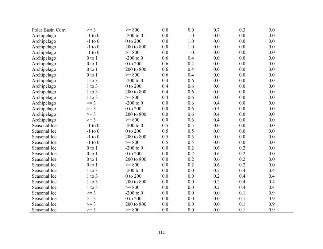
Polar Basin Conv >= 3 >= 800 0.0 0.0 0.7 0.3 0.0 Archipelago -1 to 0 -200 to 0 0.0 1.0 0.0 0.0 0.0 Archipelago -1 to 0 0 to 200 0.0 1.0 0.0 0.0 0.0 Archipelago -1 to 0 200 to 800 0.0 1.0 0.0 0.0 0.0 Archipelago -1 to 0 >= 800 0.0 1.0 0.0 0.0 0.0 Archipelago 0 to 1 -200 to 0 0.6 0.4 0.0 0.0 0.0 Archipelago 0 to 1 0 to 200 0.6 0.4 0.0 0.0 0.0 Archipelago 0 to 1 200 to 800 0.6 0.4 0.0 0.0 0.0 Archipelago 0 to 1 >= 800 0.6 0.4 0.0 0.0 0.0 Archipelago 1 to 3 -200 to 0 0.4 0.6 0.0 0.0 0.0 Archipelago 1 to 3 0 to 200 0.4 0.6 0.0 0.0 0.0 Archipelago 1 to 3 200 to 800 0.4 0.6 0.0 0.0 0.0 Archipelago 1 to 3 >= 800 0.4 0.6 0.0 0.0 0.0 Archipelago >= 3 -200 to 0 0.0 0.6 0.4 0.0 0.0 Archipelago >= 3 0 to 200 0.0 0.6 0.4 0.0 0.0 Archipelago >= 3 200 to 800 0.0 0.6 0.4 0.0 0.0 Archipelago >= 3 >= 800 0.0 0.6 0.4 0.0 0.0 Seasonal Ice -1 to 0 -200 to 0 0.5 0.5 0.0 0.0 0.0 Seasonal Ice -1 to 0 0 to 200 0.5 0.5 0.0 0.0 0.0 Seasonal Ice -1 to 0 200 to 800 0.5 0.5 0.0 0.0 0.0 Seasonal Ice -1 to 0 >= 800 0.5 0.5 0.0 0.0 0.0 Seasonal Ice 0 to 1 -200 to 0 0.0 0.2 0.6 0.2 0.0 Seasonal Ice 0 to 1 0 to 200 0.0 0.2 0.6 0.2 0.0 Seasonal Ice 0 to 1 200 to 800 0.0 0.2 0.6 0.2 0.0 Seasonal Ice 0 to 1 >= 800 0.0 0.2 0.6 0.2 0.0 Seasonal Ice 1 to 3 -200 to 0 0.0 0.0 0.2 0.4 0.4 Seasonal Ice 1 to 3 0 to 200 0.0 0.0 0.2 0.4 0.4 Seasonal Ice 1 to 3 200 to 800 0.0 0.0 0.2 0.4 0.4 Seasonal Ice 1 to 3 >= 800 0.0 0.0 0.2 0.4 0.4 Seasonal Ice >= 3 -200 to 0 0.0 0.0 0.0 0.1 0.9 Seasonal Ice >= 3 0 to 200 0.0 0.0 0.0 0.1 0.9 Seasonal Ice >= 3 200 to 800 0.0 0.0 0.0 0.1 0.9 Seasonal Ice >= 3 >= 800 0.0 0.0 0.0 0.1 0.9

112

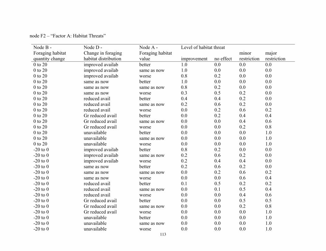
node F2 – “Factor A: Habitat Threats”

Node B - Node D - Node A - Level of habitat threat Foraging habitat Change in foraging Foraging habitat minor major quantity change habitat distribution value improvement no effect restriction restriction 0 to 20 improved availab better 1.0 0.0 0.0 0.0 0 to 20 improved availab same as now 1.0 0.0 0.0 0.0 0 to 20 improved availab worse 0.8 0.2 0.0 0.0 0 to 20 same as now better 1.0 0.0 0.0 0.0 0 to 20 same as now same as now 0.8 0.2 0.0 0.0 0 to 20 same as now worse 0.3 0.5 0.2 0.0 0 to 20 reduced avail better 0.4 0.4 0.2 0.0 0 to 20 reduced avail same as now 0.2 0.6 0.2 0.0 0 to 20 reduced avail worse 0.0 0.2 0.6 0.2 0 to 20 Gr reduced avail better 0.0 0.2 0.4 0.4 0 to 20 Gr reduced avail same as now 0.0 0.0 0.4 0.6 0 to 20 Gr reduced avail worse 0.0 0.0 0.2 0.8 0 to 20 unavailable better 0.0 0.0 0.0 1.0 0 to 20 unavailable same as now 0.0 0.0 0.0 1.0 0 to 20 unavailable worse 0.0 0.0 0.0 1.0 -20 to 0 improved availab better 0.8 0.2 0.0 0.0 -20 to 0 improved availab same as now 0.2 0.6 0.2 0.0 -20 to 0 improved availab worse 0.2 0.4 0.4 0.0 -20 to 0 same as now better 0.2 0.6 0.2 0.0 -20 to 0 same as now same as now 0.0 0.2 0.6 0.2 -20 to 0 same as now worse 0.0 0.0 0.6 0.4 -20 to 0 reduced avail better 0.1 0.5 0.2 0.2 -20 to 0 reduced avail same as now 0.0 0.1 0.5 0.4 -20 to 0 reduced avail worse 0.0 0.0 0.4 0.6 -20 to 0 Gr reduced avail better 0.0 0.0 0.5 0.5 -20 to 0 Gr reduced avail same as now 0.0 0.0 0.2 0.8 -20 to 0 Gr reduced avail worse 0.0 0.0 0.0 1.0 -20 to 0 unavailable better 0.0 0.0 0.0 1.0 -20 to 0 unavailable same as now 0.0 0.0 0.0 1.0 -20 to 0 unavailable worse 0.0 0.0 0.0 1.0

113

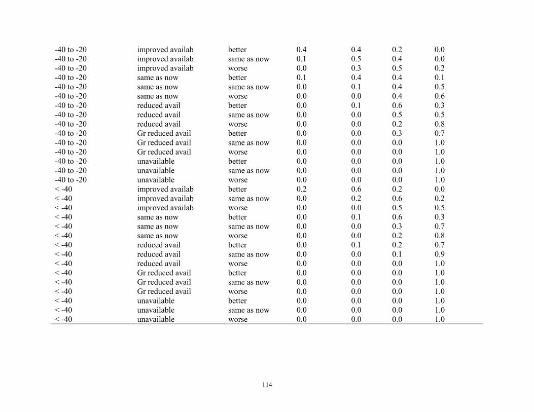
-40 to -20 improved availab better 0.4 0.4 0.2 0.0 -40 to -20 improved availab same as now 0.1 0.5 0.4 0.0 -40 to -20 improved availab worse 0.0 0.3 0.5 0.2 -40 to -20 same as now better 0.1 0.4 0.4 0.1 -40 to -20 same as now same as now 0.0 0.1 0.4 0.5 -40 to -20 same as now worse 0.0 0.0 0.4 0.6 -40 to -20 reduced avail better 0.0 0.1 0.6 0.3 -40 to -20 reduced avail same as now 0.0 0.0 0.5 0.5 -40 to -20 reduced avail worse 0.0 0.0 0.2 0.8 -40 to -20 Gr reduced avail better 0.0 0.0 0.3 0.7 -40 to -20 Gr reduced avail same as now 0.0 0.0 0.0 1.0 -40 to -20 Gr reduced avail worse 0.0 0.0 0.0 1.0 -40 to -20 unavailable better 0.0 0.0 0.0 1.0 -40 to -20 unavailable same as now 0.0 0.0 0.0 1.0 -40 to -20 unavailable worse 0.0 0.0 0.0 1.0 < -40 improved availab better 0.2 0.6 0.2 0.0 < -40 improved availab same as now 0.0 0.2 0.6 0.2 < -40 improved availab worse 0.0 0.0 0.5 0.5 < -40 same as now better 0.0 0.1 0.6 0.3 < -40 same as now same as now 0.0 0.0 0.3 0.7 < -40 same as now worse 0.0 0.0 0.2 0.8 < -40 reduced avail better 0.0 0.1 0.2 0.7 < -40 reduced avail same as now 0.0 0.0 0.1 0.9 < -40 reduced avail worse 0.0 0.0 0.0 1.0 < -40 Gr reduced avail better 0.0 0.0 0.0 1.0 < -40 Gr reduced avail same as now 0.0 0.0 0.0 1.0 < -40 Gr reduced avail worse 0.0 0.0 0.0 1.0 < -40 unavailable better 0.0 0.0 0.0 1.0 < -40 unavailable same as now 0.0 0.0 0.0 1.0 < -40 unavailable worse 0.0 0.0 0.0 1.0

114

node C1 – “Human disturbance”

Node B1 - Node J - Node R1 - Node J1- Level of human disturbance Bear-human Oil & gas same greatly interactions Shipping activity Tourism reduced as now elevated elevated increased increased increase increased 0.0 0.0 0.0 1.0 increased increased increase same as now 0.0 0.0 0.0 1.0 increased increased increase decreased 0.0 0.0 0.1 0.9 increased increased no change increased 0.0 0.0 0.0 1.0 increased increased no change same as now 0.0 0.0 0.1 0.9 increased increased no change decreased 0.0 0.0 0.2 0.8 increased increased decrease increased 0.0 0.0 0.3 0.7 increased increased decrease same as now 0.0 0.0 0.6 0.4 increased increased decrease decreased 0.0 0.0 0.5 0.5 increased same as now increase increased 0.0 0.0 0.0 1.0 increased same as now increase same as now 0.0 0.0 0.2 0.8 increased same as now increase decreased 0.0 0.0 0.3 0.7 increased same as now no change increased 0.0 0.0 0.5 0.5 increased same as now no change same as now 0.0 0.0 0.7 0.3 increased same as now no change decreased 0.0 0.2 0.6 0.2 increased same as now decrease increased 0.0 0.0 0.7 0.3 increased same as now decrease same as now 0.0 0.2 0.7 0.1 increased same as now decrease decreased 0.0 0.4 0.6 0.0 same as now increased increase increased 0.0 0.0 0.2 0.8 same as now increased increase same as now 0.0 0.0 0.5 0.5 same as now increased increase decreased 0.0 0.2 0.6 0.2 same as now increased no change increased 0.0 0.2 0.8 0.0 same as now increased no change same as now 0.0 0.3 0.7 0.0 same as now increased no change decreased 0.0 0.5 0.5 0.0 same as now increased decrease increased 0.0 0.3 0.7 0.0 same as now increased decrease same as now 0.0 0.5 0.5 0.0 same as now increased decrease decreased 0.0 0.6 0.4 0.0 same as now same as now increase increased 0.0 0.2 0.8 0.0 same as now same as now increase same as now 0.0 0.4 0.6 0.0 same as now same as now increase decreased 0.0 0.5 0.5 0.0 same as now same as now no change increased 0.0 0.8 0.2 0.0

115

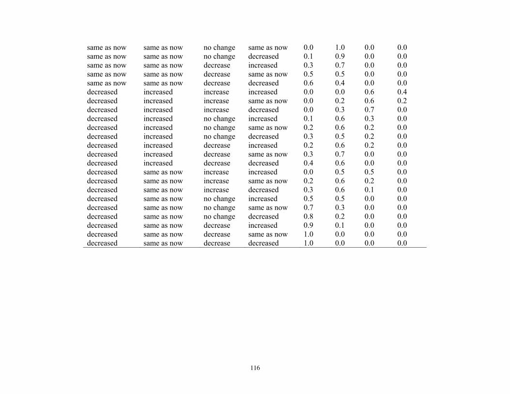
same as now same as now no change same as now 0.0 1.0 0.0 0.0 same as now same as now no change decreased 0.1 0.9 0.0 0.0 same as now same as now decrease increased 0.3 0.7 0.0 0.0 same as now same as now decrease same as now 0.5 0.5 0.0 0.0 same as now same as now decrease decreased 0.6 0.4 0.0 0.0 decreased increased increase increased 0.0 0.0 0.6 0.4 decreased increased increase same as now 0.0 0.2 0.6 0.2 decreased increased increase decreased 0.0 0.3 0.7 0.0 decreased increased no change increased 0.1 0.6 0.3 0.0 decreased increased no change same as now 0.2 0.6 0.2 0.0 decreased increased no change decreased 0.3 0.5 0.2 0.0 decreased increased decrease increased 0.2 0.6 0.2 0.0 decreased increased decrease same as now 0.3 0.7 0.0 0.0 decreased increased decrease decreased 0.4 0.6 0.0 0.0 decreased same as now increase increased 0.0 0.5 0.5 0.0 decreased same as now increase same as now 0.2 0.6 0.2 0.0 decreased same as now increase decreased 0.3 0.6 0.1 0.0 decreased same as now no change increased 0.5 0.5 0.0 0.0 decreased same as now no change same as now 0.7 0.3 0.0 0.0 decreased same as now no change decreased 0.8 0.2 0.0 0.0 decreased same as now decrease increased 0.9 0.1 0.0 0.0 decreased same as now decrease same as now 1.0 0.0 0.0 0.0 decreased same as now decrease decreased 1.0 0.0 0.0 0.0

116

node C2 – “Pollution”

Node R4 - Node T1 - Level of pollution Hydrocarbons / oil same greatly spill Contaminants reduced as now elevated elevated increased occurr elevated 0.0 0.0 0.0 1.0 increased occurr same as now 0.0 0.0 0.6 0.4 increased occurr reduced 0.0 0.4 0.4 0.2 same as now elevated 0.0 0.3 0.7 0.0 same as now same as now 0.0 1.0 0.0 0.0 same as now reduced 0.4 0.6 0.0 0.0 decreased occurr elevated 0.3 0.5 0.2 0.0 decreased occurr same as now 0.8 0.2 0.0 0.0 decreased occurr reduced 1.0 0.0 0.0 0.0

node A6 – “Factor E. Other factors natural or man-made”

Node C1 - Node C2 - Level of other factors minor major

C1 C2 improvement no effect restrictio restrictio reduced reduced 1.0 0.0 0.0 0.0 reduced same as now 1.0 0.0 0.0 0.0 reduced elevated 0.3 0.4 0.3 0.0 reduced greatly elevated 0.0 0.3 0.3 0.4 same as now reduced 0.6 0.4 0.0 0.0 same as now same as now 0.0 1.0 0.0 0.0 same as now elevated 0.0 0.4 0.6 0.0 same as now greatly elevated 0.0 0.2 0.2 0.6 elevated reduced 0.0 0.2 0.5 0.3 elevated same as now 0.0 0.0 0.5 0.5 elevated elevated 0.0 0.0 0.4 0.6 elevated greatly elevated 0.0 0.0 0.3 0.7 greatly elevated reduced 0.0 0.0 0.3 0.7 greatly elevated same as now 0.0 0.0 0.2 0.8 greatly elevated elevated 0.0 0.0 0.1 0.9 greatly elevated greatly elevated 0.0 0.0 0.0 1.0

117

node C3 – “Distribution Response”

Node F2 -Factor A. Habitat

Node A6 -Factor E. Other factors

Node G - Relocation

Distribution response same reduced transient

Threats improvement improvement improvement improvement improvement improvement improvement improvement no effect no effect no effect

(natural or man-made) improvement improvement no effect no effect minor restrictio minor restrictio major restrictio major restrictio improvement improvement no effect

possible Yes No Yes No Yes No Yes No Yes No Yes

as now 1.0 1.0 1.0 1.0 0.9 0.9 0.8 0.8 1.0 1.0 1.0

but resi 0.0 0.0 0.0 0.0 0.1 0.1 0.1 0.2 0.0 0.0 0.0

visito0.0 0.0 0.0 0.0 0.0 0.0 0.1 0.0 0.0 0.0 0.0

extirpated 0.0 0.0 0.0 0.0 0.0 0.0 0.0 0.0 0.0 0.0 0.0

no effect no effect No 1.0 0.0 0.0 0.0 no effect minor restrictio Yes 0.8 0.1 0.1 0.0 no effect minor restrictio No 0.8 0.2 0.0 0.0 no effect no effect minor restrictio minor restrictio minor restrictio

major restrictio major restrictio improvement improvement no effect

Yes No Yes No Yes

0.5 0.5 0.5 0.5 0.4

0.2 0.5 0.25 0.5 0.3

0.3 0.0 0.25 0.0 0.3

0.0 0.0 0.0 0.0 0.0

minor restrictio no effect No 0.4 0.6 0.0 0.0 minor restrictio minor restrictio Yes 0.3 0.3 0.4 0.0 minor restrictio minor restrictio No 0.3 0.6 0.0 0.1 minor restrictio minor restrictio major restrictio major restrictio major restrictio major restrictio major restrictio major restrictio major restrictio major restrictio

major restrictio major restrictio improvement improvement no effect no effect minor restrictio minor restrictio major restrictio major restrictio

Yes No Yes No Yes No Yes No Yes No

0.2 0.2 0.0 0.0 0.0 0.0 0.0 0.0 0.0 0.0

0.2 0.5 0.3 0.3 0.2 0.2 0.1 0.1 0.0 0.0

0.6 0.0 0.35 0.0 0.4 0.0 0.45 0.0 0.3 0.0

0.0 0.3 0.35 0.7 0.4 0.8 0.45 0.9 0.7 1.0

118

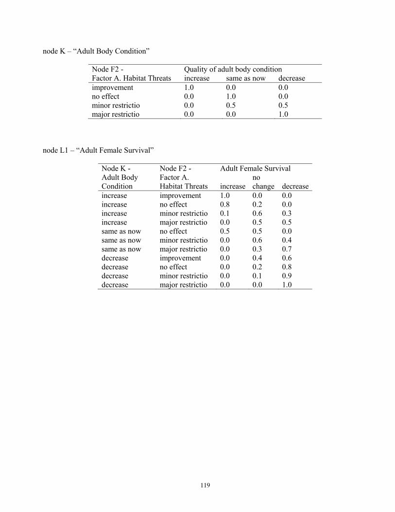
node K – “Adult Body Condition”

Node F2 - Quality of adult body condition Factor A. Habitat Threats increase same as now decrease improvement 1.0 0.0 0.0 no effect 0.0 1.0 0.0 minor restrictio 0.0 0.5 0.5 major restrictio 0.0 0.0 1.0

node L1 – “Adult Female Survival”

Node K - Node F2 - Adult Female Survival Adult Body Factor A. no Condition Habitat Threats increase change decrease increase improvement 1.0 0.0 0.0 increase no effect 0.8 0.2 0.0 increase minor restrictio 0.1 0.6 0.3 increase major restrictio 0.0 0.5 0.5 same as now no effect 0.5 0.5 0.0 same as now minor restrictio 0.0 0.6 0.4 same as now major restrictio 0.0 0.3 0.7 decrease improvement 0.0 0.4 0.6 decrease no effect 0.0 0.2 0.8 decrease minor restrictio 0.0 0.1 0.9 decrease major restrictio 0.0 0.0 1.0

119

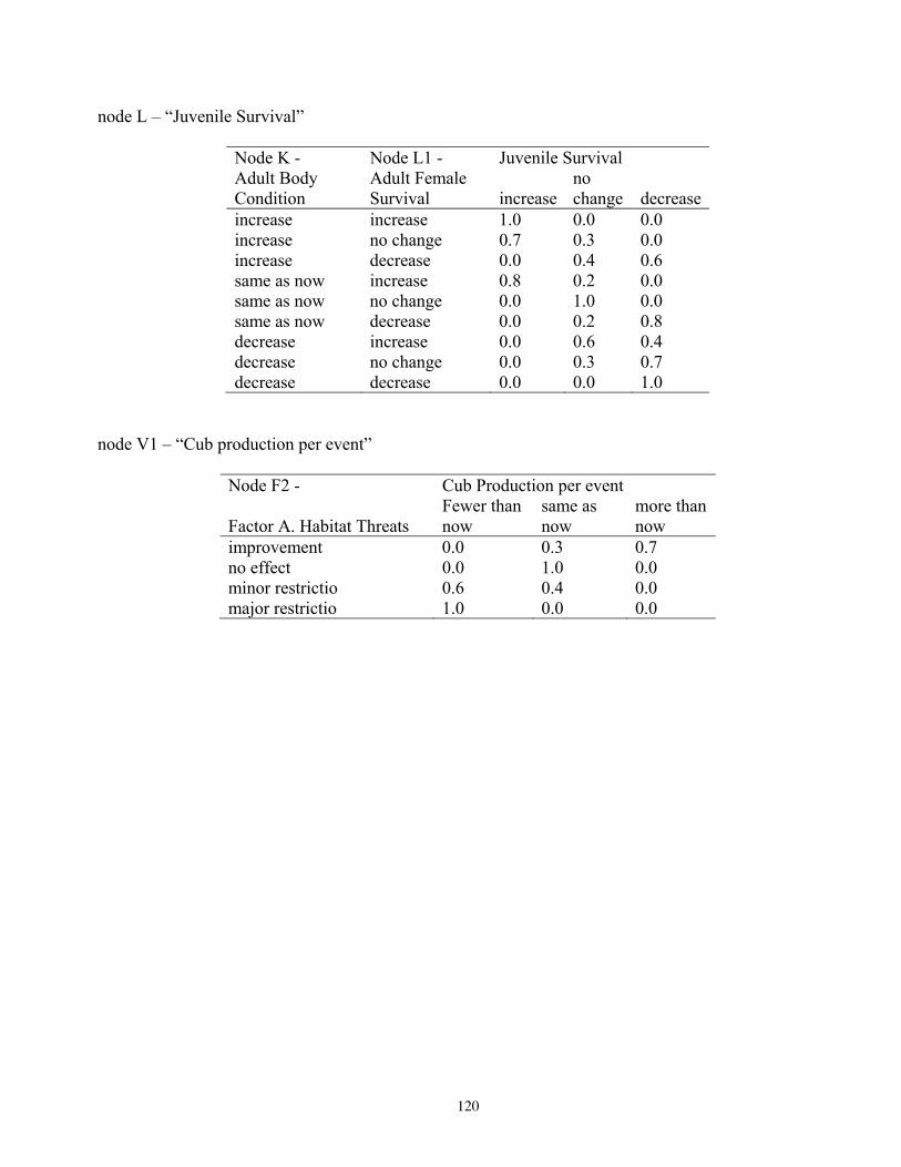
node L – “Juvenile Survival”

Node K - Node L1 - Juvenile Survival Adult Body Adult Female no Condition Survival increase change decrease increase increase 1.0 0.0 0.0 increase no change 0.7 0.3 0.0 increase decrease 0.0 0.4 0.6 same as now increase 0.8 0.2 0.0 same as now no change 0.0 1.0 0.0 same as now decrease 0.0 0.2 0.8 decrease increase 0.0 0.6 0.4 decrease no change 0.0 0.3 0.7 decrease decrease 0.0 0.0 1.0

node V1 – “Cub production per event”

Node F2 - Cub Production per event Fewer than same as more than

Factor A. Habitat Threats now now now improvement 0.0 0.3 0.7 no effect 0.0 1.0 0.0 minor restrictio 0.6 0.4 0.0 major restrictio 1.0 0.0 0.0

120

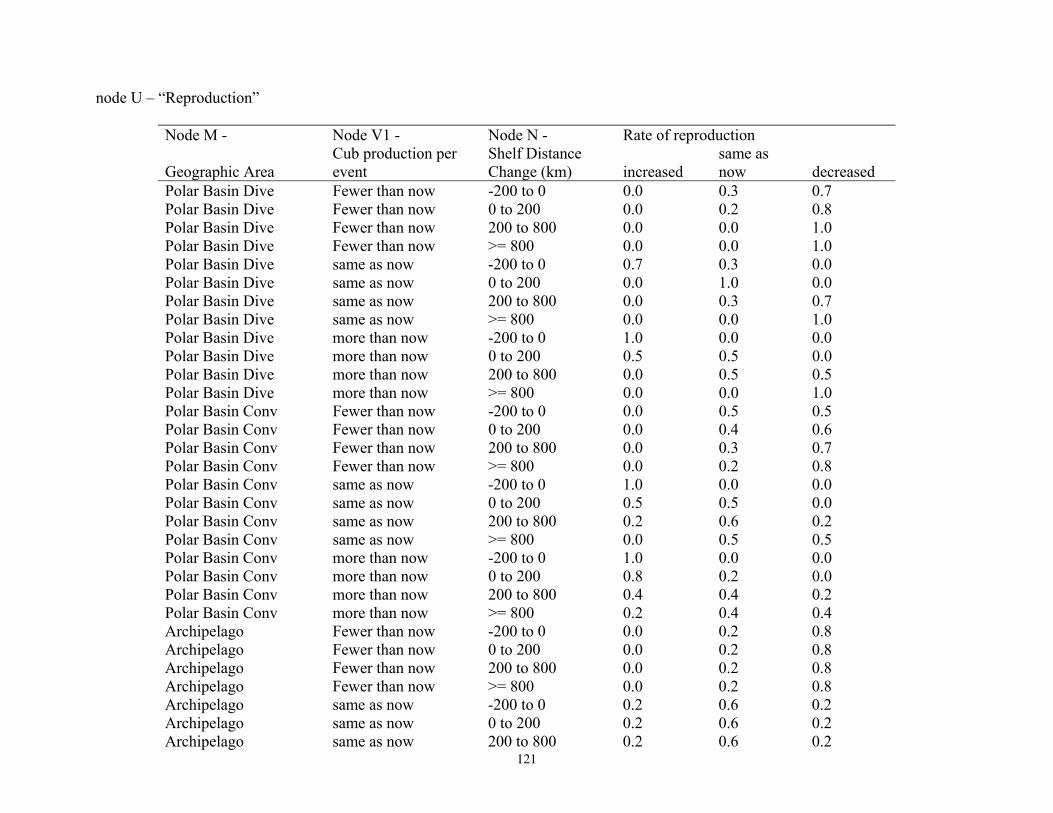
node U – “Reproduction”

Node M - Node V1 - Node N - Rate of reproduction Cub production per Shelf Distance same as

Geographic Area event Change (km) increased now decreased Polar Basin Dive Fewer than now -200 to 0 0.0 0.3 0.7 Polar Basin Dive Fewer than now 0 to 200 0.0 0.2 0.8 Polar Basin Dive Fewer than now 200 to 800 0.0 0.0 1.0 Polar Basin Dive Fewer than now >= 800 0.0 0.0 1.0 Polar Basin Dive same as now -200 to 0 0.7 0.3 0.0 Polar Basin Dive same as now 0 to 200 0.0 1.0 0.0 Polar Basin Dive same as now 200 to 800 0.0 0.3 0.7 Polar Basin Dive same as now >= 800 0.0 0.0 1.0 Polar Basin Dive more than now -200 to 0 1.0 0.0 0.0 Polar Basin Dive more than now 0 to 200 0.5 0.5 0.0 Polar Basin Dive more than now 200 to 800 0.0 0.5 0.5 Polar Basin Dive more than now >= 800 0.0 0.0 1.0 Polar Basin Conv Fewer than now -200 to 0 0.0 0.5 0.5 Polar Basin Conv Fewer than now 0 to 200 0.0 0.4 0.6 Polar Basin Conv Fewer than now 200 to 800 0.0 0.3 0.7 Polar Basin Conv Fewer than now >= 800 0.0 0.2 0.8 Polar Basin Conv same as now -200 to 0 1.0 0.0 0.0 Polar Basin Conv same as now 0 to 200 0.5 0.5 0.0 Polar Basin Conv same as now 200 to 800 0.2 0.6 0.2 Polar Basin Conv same as now >= 800 0.0 0.5 0.5 Polar Basin Conv more than now -200 to 0 1.0 0.0 0.0 Polar Basin Conv more than now 0 to 200 0.8 0.2 0.0 Polar Basin Conv more than now 200 to 800 0.4 0.4 0.2 Polar Basin Conv more than now >= 800 0.2 0.4 0.4 Archipelago Fewer than now -200 to 0 0.0 0.2 0.8 Archipelago Fewer than now 0 to 200 0.0 0.2 0.8 Archipelago Fewer than now 200 to 800 0.0 0.2 0.8 Archipelago Fewer than now >= 800 0.0 0.2 0.8 Archipelago same as now -200 to 0 0.2 0.6 0.2 Archipelago same as now 0 to 200 0.2 0.6 0.2 Archipelago same as now 200 to 800 0.2 0.6 0.2

121

Archipelago same as now Archipelago more than now Archipelago more than now Archipelago more than now Archipelago more than now Seasonal Ice Fewer than now Seasonal Ice Fewer than now Seasonal Ice Fewer than now Seasonal Ice Fewer than now Seasonal Ice same as now Seasonal Ice same as now Seasonal Ice same as now Seasonal Ice same as now Seasonal Ice more than now Seasonal Ice more than now Seasonal Ice more than now Seasonal Ice more than now

>= 800

-200 to 0

0 to 200

200 to 800

>= 800

-200 to 0

0 to 200

200 to 800

>= 800

-200 to 0

0 to 200

200 to 800

>= 800

-200 to 0

0 to 200

200 to 800

>= 800

0.2 0.8 0.8 0.8 0.8 0.0 0.0 0.0 0.0 0.2 0.2 0.2 0.2 0.8 0.8 0.8 0.8

0.6 0.2 0.2 0.0 0.2 0.0 0.2 0.0 0.2 0.0 0.2 0.8 0.2 0.8 0.2 0.8 0.2 0.8 0.6 0.2 0.6 0.2 0.6 0.2 0.6 0.2 0.2 0.0 0.2 0.0 0.2 0.0 0.2 0.0

122

node L2 – “Vital Rates”

Node L1 - Node L - Node U - Vital Rates Adult Female Juvenile same Surival Survival Reproduction improve as now decline increase increase increased 1.0 0.0 0.0 increase increase same as now 1.0 0.0 0.0 increase increase decreased 0.6 0.4 0.0 increase no change increased 0.9 0.1 0.0 increase no change same as now 0.8 0.2 0.0 increase no change decreased 0.7 0.2 0.1 increase decrease increased 0.3 0.5 0.2 increase decrease same as now 0.2 0.5 0.3 increase decrease decreased 0.0 0.4 0.6 no change increase increased 0.7 0.3 0.0 no change increase same as now 0.6 0.4 0.0 no change increase decreased 0.2 0.5 0.3 no change no change increased 0.2 0.8 0.0 no change no change same as now 0.0 1.0 0.0 no change no change decreased 0.0 0.8 0.2 no change decrease increased 0.0 0.6 0.4 no change decrease same as now 0.0 0.5 0.5 no change decrease decreased 0.0 0.3 0.7 decrease increase increased 0.2 0.4 0.4 decrease increase same as now 0.0 0.6 0.4 decrease increase decreased 0.0 0.5 0.5 decrease no change increased 0.1 0.5 0.4 decrease no change same as now 0.0 0.4 0.6 decrease no change decreased 0.0 0.3 0.7 decrease decrease increased 0.0 0.2 0.8 decrease decrease same as now 0.0 0.0 1.0 decrease decrease decreased 0.0 0.0 1.0

123

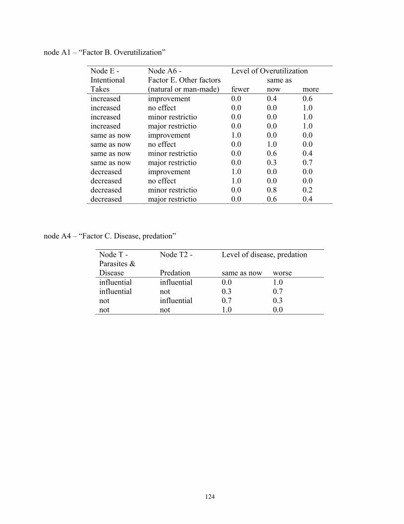
node A1 – “Factor B. Overutilization”

Node E - Node A6 - Level of Overutilization Intentional Factor E. Other factors same as Takes (natural or man-made) fewer now more increased improvement 0.0 0.4 0.6 increased no effect 0.0 0.0 1.0 increased minor restrictio 0.0 0.0 1.0 increased major restrictio 0.0 0.0 1.0 same as now improvement 1.0 0.0 0.0 same as now no effect 0.0 1.0 0.0 same as now minor restrictio 0.0 0.6 0.4 same as now major restrictio 0.0 0.3 0.7 decreased improvement 1.0 0.0 0.0 decreased no effect 1.0 0.0 0.0 decreased minor restrictio 0.0 0.8 0.2 decreased major restrictio 0.0 0.6 0.4

node A4 – “Factor C. Disease, predation”

Node T - Node T2 - Level of disease, predation Parasites & Disease Predation same as now worse influential influential 0.0 1.0 influential not 0.3 0.7 not influential 0.7 0.3 not not 1.0 0.0

124

node C4 – “Numerical Response”

Node L2 - Node A1 - Node A4 - Numerical Response Factor B. Factor C. Disease, increased same reduced

Vital Rates Overutilization Predation densit as now density rare absent improve fewer same as now 1.0 0.0 0.0 0.0 0.0 improve fewer worse 0.5 0.25 0.25 0.0 0.0 improve same as now same as now 0.8 0.2 0.0 0.0 0.0 improve same as now worse 0.5 0.25 0.25 0.0 0.0 improve more same as now 0.3 0.35 0.35 0.0 0.0 improve more worse 0.1 0.4 0.5 0.0 0.0 same as now fewer same as now 0.2 0.8 0.0 0.0 0.0 same as now fewer worse 0.0 0.8 0.2 0.0 0.0 same as now same as now same as now 0.0 1.0 0.0 0.0 0.0 same as now same as now worse 0.0 0.3 0.7 0.0 0.0 same as now more same as now 0.0 0.2 0.8 0.0 0.0 same as now more worse 0.0 0.0 1.0 0.0 0.0 decline fewer same as now 0.0 0.5 0.5 0.0 0.0 decline fewer worse 0.0 0.3 0.7 0.0 0.0 decline same as now same as now 0.0 0.0 1.0 0.0 0.0 decline same as now worse 0.0 0.0 0.75 0.25 0.0 decline more same as now 0.0 0.0 0.4 0.4 0.2 decline more worse 0.0 0.0 0.2 0.4 0.4

125

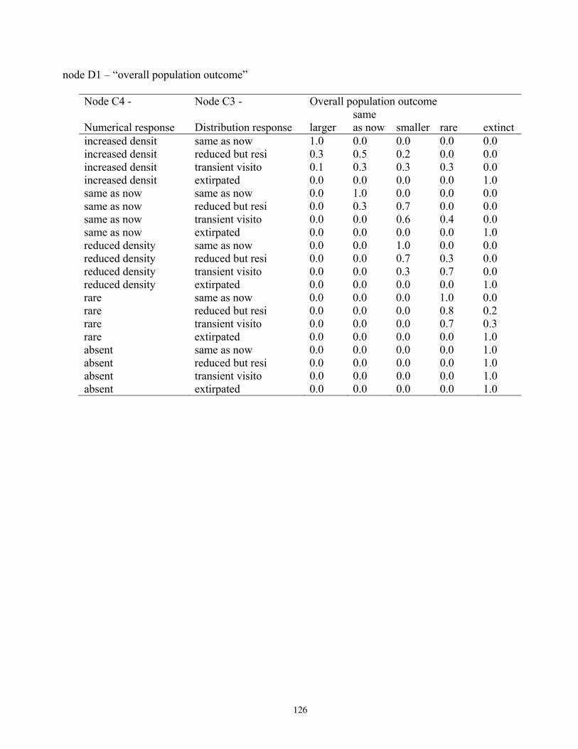
node D1 – “overall population outcome”

Node C4 - Node C3 - Overall population outcome same

Numerical response Distribution response larger as now smaller rare extinct increased densit same as now 1.0 0.0 0.0 0.0 0.0 increased densit reduced but resi 0.3 0.5 0.2 0.0 0.0 increased densit transient visito 0.1 0.3 0.3 0.3 0.0 increased densit extirpated 0.0 0.0 0.0 0.0 1.0 same as now same as now 0.0 1.0 0.0 0.0 0.0 same as now reduced but resi 0.0 0.3 0.7 0.0 0.0 same as now transient visito 0.0 0.0 0.6 0.4 0.0 same as now extirpated 0.0 0.0 0.0 0.0 1.0 reduced density same as now 0.0 0.0 1.0 0.0 0.0 reduced density reduced but resi 0.0 0.0 0.7 0.3 0.0 reduced density transient visito 0.0 0.0 0.3 0.7 0.0 reduced density extirpated 0.0 0.0 0.0 0.0 1.0 rare same as now 0.0 0.0 0.0 1.0 0.0 rare reduced but resi 0.0 0.0 0.0 0.8 0.2 rare transient visito 0.0 0.0 0.0 0.7 0.3 rare extirpated 0.0 0.0 0.0 0.0 1.0 absent same as now 0.0 0.0 0.0 0.0 1.0 absent reduced but resi 0.0 0.0 0.0 0.0 1.0 absent transient visito 0.0 0.0 0.0 0.0 1.0 absent extirpated 0.0 0.0 0.0 0.0 1.0

126