Forecasting the Term Structure of Interest Rates:

A Bayesian Dynamic Graphical Modeling Approach

by

John Charles Lazzaro

Department of Statistical ScienceDuke University

Date:Approved:

Mike West, Supervisor

Merlise A. Clyde

Galen Reeves

Thesis submitted in partial fulfillment of the requirements for the degree ofMaster of Science in the Department of Statistical Science

in the Graduate School of Duke University2019

Abstract

Forecasting the Term Structure of Interest Rates:

A Bayesian Dynamic Graphical Modeling Approach

by

John Charles Lazzaro

Department of Statistical ScienceDuke University

Date:Approved:

Mike West, Supervisor

Merlise A. Clyde

Galen Reeves

An abstract of a thesis submitted in partial fulfillment of the requirements forthe degree of Master of Science in the Department of Statistical Science

in the Graduate School of Duke University2019

Copyright c© 2019 by John Charles LazzaroAll rights reserved except the rights granted by the

Creative Commons Attribution-Noncommercial Licence

Abstract

This thesis addresses the financial econometric problem of forecasting the term struc-

ture of interest rates by using classes of Dynamic Dependence Network Models

(DDNMs). This Bayesian econometric framework defines structured dynamic graph-

ical models for multivariate time series that utilize a hierarchical, contemporaneous

dependence structure across series augmented with time-varying autoregressive com-

ponents. Using yield and macroeconomic data from the post-Volcker era, various such

models are explored and evaluated. On the basis of economic reasoning and empir-

ical statistical evaluations, we specify an interpretable model which outperforms a

standard time-varying vector autoregressive model in forecast accuracy particularly

at longer horizons relevant for economic policy considerations. In particular, the

chosen model reduces forecast error metrics and produces stable forecast trajectories

for yields on U.S. Treasuries up to 12 months ahead. The out-of-sample performance

of the DDNM is robust to changes in model specification, hyper-parameter choices,

and exogenous macroeconomic information sets. The analysis highlights the utility

of this class of models and suggests next steps in research and development in this

area of Bayesian macroeconomics.

iv

Contents

Abstract iv

List of Tables vii

List of Figures viii

Acknowledgements ix

1 Introduction 1

2 Models & Data 5

2.1 Data . . . . . . . . . . . . . . . . . . . . . . . . . . . . . . . . . . . . 5

2.2 Models . . . . . . . . . . . . . . . . . . . . . . . . . . . . . . . . . . . 6

2.2.1 Exchangeable Model . . . . . . . . . . . . . . . . . . . . . . . 6

2.2.2 Dynamic Dependence Network Model . . . . . . . . . . . . . . 7

3 Forecasting 15

3.1 TV-VAR vs. DDNM . . . . . . . . . . . . . . . . . . . . . . . . . . . 15

3.2 DDNM Specification . . . . . . . . . . . . . . . . . . . . . . . . . . . 18

3.2.1 Parental Sets and Discount Factors . . . . . . . . . . . . . . . 20

3.2.2 Exogenous Predictors . . . . . . . . . . . . . . . . . . . . . . . 25

4 Conclusion 31

A Supplementary Tables & Figures 34

B DDNM Sample Code 41

v

Bibliography 45

vi

List of Tables

2.1 DDNM Structure . . . . . . . . . . . . . . . . . . . . . . . . . . . . . 14

3.1 DDNM/TV-VAR: Forecast summaries . . . . . . . . . . . . . . . . . 17

A.1 Macroeconomic Predictors: Description . . . . . . . . . . . . . . . . . 35

A.2 DDNM Structure: Non-Parsimonious Parental Sets . . . . . . . . . . 35

A.3 DDNM Structure: Macroeconomic Predictors . . . . . . . . . . . . . 36

A.4 Parental Sets/Discount Factors: Forecast Summaries . . . . . . . . . 37

A.5 Macroeconomic Predictors: Forecast Summaries . . . . . . . . . . . . 39

vii

List of Figures

2.1 The Yield Curve over Time . . . . . . . . . . . . . . . . . . . . . . . 6

2.2 Selection of Smoothed TV-VAR(2) coefficients for 10-yr yield . . . . . 8

3.1 TV-VAR Forecast Trajectories . . . . . . . . . . . . . . . . . . . . . . 16

3.2 DDNM Forecast Trajectories . . . . . . . . . . . . . . . . . . . . . . . 19

3.3 Parental Sets/Discount Factors: Model Comparison . . . . . . . . . . 22

3.4 Parental Sets/Discount Factors: 12-step ahead forecast trajectories bymodel . . . . . . . . . . . . . . . . . . . . . . . . . . . . . . . . . . . 24

3.5 Macroeconomic Predictors: Model Comparison . . . . . . . . . . . . . 27

3.6 Macroeconomic Predictors: 12-step ahead forecast trajectories by model 28

A.1 Parental Sets/Discount Factors: 6-step ahead forecast trajectories bymodel . . . . . . . . . . . . . . . . . . . . . . . . . . . . . . . . . . . 38

A.2 Macroeconomic Predictors: 6-step ahead forecast trajectories by model 40

viii

Acknowledgements

I’d like to thank my advisor, Mike West, whose guidance has been integral to the

completion of this thesis, Merlise A. Clyde and Galen Reeves for serving on my thesis

committee, as well as the professors in the Department of Statistical Science whose

instruction has enriched my academic development. Lastly, to my parents: your

enduring selflessness, accomplishment, and unconditional love serve as an example

which I strive to emulate.

ix

1

Introduction

Forecasting yields on zero-coupon U.S. Treasuries of differing maturities is of consid-

erable interest given that yields on long-term Treasury bonds reflect, among other

things, investors’ expectations about future economic growth. Moreover, the rela-

tionship between Treasury yields of differing maturities, know as the term structure

or yield curve, is of great import as spreads between short- and long-term rates serve

as a particularly powerful predictor of a future economic recession. Therefore, pro-

ducing accurate forecasts of the term structure at a variety of forecast horizons is

an important exercise relevant for both bond portfolio management and monetary

policy decisions.

However, forecasting the term structure of interest rates is a complex, high-

dimensional problem involving fitting and predicting the evolution of a cross-section

of Treasury yields of differing maturities over time. To mitigate this complication,

traditional term structure modeling proceeds by decomposing yields into latent fac-

tors, the specification and evolution of which are broadly classified into two sets of

models. The first are purely statistical models which build upon the Nelson and

Siegel (1987) approach of parsimoniously modeling the term structure via a set of

1

smooth exponential basis functions. Notably, Diebold and Li (2006) extend this

framework to a dynamic three-factor model, and show that the latent factors corre-

spond to the level, slope, and curvature of the yield curve. This latter specification

has been augmented to study interactions between the yield curve and macroeco-

nomic conditions (Diebold et al., 2006; Moench, 2012), as well as allow for time-

varying hyper-parameters in the dynamic Nelson-Siegel factor loadings (Koopman

et al., 2010).

Though these models are tractable and produce accurate forecasts, they lack an

explicit connection to economic and finance theory regarding the term structure of

interest rates. This motivates the second class of models known as no-arbitrage affine

term structure models (ATSM) which incorporate economic theory into the statistical

methodology through the enforcement of a no-arbitrage restriction in bond markets.

Introduced by Duffie and Kan (1996) and expounded upon by Dai and Singleton

(2000), Duffee (2002), and Ang and Piazzesi (2003), these models postulate that

yields are an affine function of a set of underlying latent factors which are often

augmented with macroeconomic information when describing the dynamics of the

model (Ang and Piazzesi, 2003; Ang et al., 2004; Moench, 2008; Chib and Ergashev,

2009). These factors, in tandem with variables capturing the market prices of risk

define a stochastic discount factor mt`1 which establishes the relationship between

bond prices absent arbitrage opportunities. Namely, under the assumption of no-

arbitrage, the price of an n-period zero-coupon bond at time t, denoted ppnqt , conforms

to the following rule: ppnqt “ Et

”

mt`1ppn´1qt`1

ı

Under a particular set of assumptions concerning the functional form of the dis-

count factor mt`1, Ang and Piazzesi (2003) show that, in discrete time, bond prices

are exponential affine functions of a set of factors:

ppnqt “ exp pAn `B1

nFtq

2

Moreover, the parameters of this affine function are obtained by a set of vector differ-

ence equations which are themselves functions of a set of structural parameters of the

ATSM. More specifically, An and Bn are scalar and vector quantities, respectively,

obeying the recursive equations:

An`1 “ An `B1n p´ΩΛ0q `

1

2B1

nΩΩ1Bn ´ δ0

B1n`1 “ B1

n pΨ´ΩΛ1q ´ δ11

These equations imply an explicit dependence structure for contemporaneous bond

yields, given by: ypnqt “ ´ln

´

ppnqt

¯

n “ ´ 1npAn `B1

nFtq. Namely, given that the

parameters describing yields on shorter maturities inform those on longer maturities,

information pertaining to short-term yields propagates through the term structure

to long-term yields at a given time t.

Modeling the term structure of interest rates via a set of underlying factors is

advantageous in that it reduces the dimension of the forecasting problem while cap-

turing the dynamics of the yield curve. However, such models sacrifice some level

of economic interpretability as a result of the dimension reduction. While a neces-

sary trade-off if the primary modeling objective is forecasting future term structures,

these models are limited in their ability to deduce underlying economic relationships.

Conversely, multivariate statistical models maintain their interpretability but suffer

from degradations in computational efficiency and out-of-sample performance as the

dimension of the problem increases. Therefore, it is necessary to apply scalable

multivariate statistical models to the problem of forecasting the term structure of

interest rates in order to maximize the utility of the out-of-sample exercise.

With this in mind, this paper forecasts yields on a set of zero-coupon U.S. Trea-

suries of varying maturities using a Dynamic Dependence Network Model (Zhao

et al., 2016). This multivariate dynamic graphical model specifies a hierarchical con-

3

temporaneous dependence structure across series in order to facilitate forecasting

high-dimensional time series. Of key interest is whether utilizing this structure, re-

flected in the aforementioned contemporaneous relationship across yields implied by

the ATSM, produces substantive gains in forecasting performance relative to conven-

tional multivariate exchangeable models. The remainder of this paper is organized

as follows: Chapter 2 describes the data and models used in the forecasting exercise,

Chapter 3 summarizes the out-of-sample performance of each model, and Chapter 4

offers summary comments and future extensions.

4

2

Models & Data

2.1 Data

The dataset used in this paper consists of monthly yield and macroeconomic data for

the U.S. from 1983:01 to 2018:10 pn “ 430q which spans the post-Volcker disinflation

era to the present. We choose this window since prior to the Great Recession of

2008 this period is marked by a stable, consistent monetary policy regime. The

term structure data used are yields of Constant Maturity Treasury (CMT) securities

complied from the FRED II database for maturities of 1, 3, 6, and 12 months, as

well as 2, 5, and 10 years. As suggested by Ang and Piazzesi (2003), among others,

the effective federal funds rate is used as a proxy for the 1-month Treasury yield.

We consider a subset of the broad panel of macroeconomic variables complied by

Giannone et al. (2004) as exogenous predictors in the analysis. Following Giannone

et al. (2004), we transform these variable into their quarterly differences or annualized

quarterly growth rates reflecting the notion that monetary policy decisions and bond

market conditions respond to relative changes in macroeconomic conditions. Variable

descriptions and transformations are summarized in Table A.1.

5

Figure 2.1: The Yield Curve over Time

2.2 Models

2.2.1 Exchangeable Model

We first model the term structure of interest rates using a time-varying vector au-

toregressive (TV-VAR) model of order d with a level mean on the vector of yields:

y1t “ pyp120qt , y

p60qt , y

p24qt , y

p12qt , y

p6qt , y

p3qt , y

p1qt q

A special case of an exchangeable multivariate dynamic linear model (DLM) with a

Wishart discount model of multivariate stochastic volatility (Prado and West, 2010,

Ch. 9,10), this model represents the vector of yields as a function of its past values:

yt “ µt `

dÿ

j“1

Φjtyt´j ` νt νt „ Np0,Vtq

6

The model order d “ 2 as well as the relevant discount factors for the state matrix

and multivariate stochastic volatility model pδ, βq “ p0.99, 0.95q were selected from

a grid of values d P r1, 6s, pδ, βq P r0.94, 0.99s2 to maximize the cumulative log-

likelihood of the one-step ahead predictive density. We note that the grid of values

for the discount factors is constrained to relatively high values since we are interested

in producing multiple step-ahead forecasts. We use non-informative priors wherein

we set the level µ0 to be the mean of the data, the TV-VAR coefficients to be zero

everywhere but the first lag of the same series which is set to 0.9, and posit no

initial correlation across yields. Furthermore, when training the model we treat the

first two years of observations as prior information as the stable monetary policy at

the beginning of the post-Volcker era allows the model to train on a conventional

term structure. While this is immaterial for the forward filtering procedure, it does

constrain the number of time points for which we have smoothed coefficient estimates

pn “ 404q, a selection of which are reported in Figure 2.2. Upon the inclusion of

the level mean, none of the exogenous macroeconomic covariates included in this

exchangeable model exhibit statistically significant smoothed coefficient estimates

throughout time. This result is robust to changes in the initial prior information,

and thus we do not include any exogenous covariates in this model.

2.2.2 Dynamic Dependence Network Model

Due to issues regarding the scalability of the TV-VAR model and the limitation

that the same set of covariates must be used across series in multivariate exchange-

able models, we alternatively use a Dynamic Dependence Network Model (DDNM)

to model the term structure of interest rates. An extension of a multiregression

dynamic model (MDM), DDNMs permit both contemporaneous and lagged dy-

namic linkages across series. The broader class of MDMs impose a hierarchical

contemporaneous conditional dependence structure across series which allows for

7

Figure 2.2: Selection of Smoothed TV-VAR(2) coefficients for 10-yr yield

a triangular/Cholesky-style specification of the resulting dynamic graphical model.

This feature facilitates modeling higher numbers of individual time series as each

univariate series can be decoupled for sequential analysis and then recoupled for

multivariate forecasting and analysis. While the reader is referred to Zhao et al.

(2016) for a full discussion, we summarize the relevant details and underlying theory

below.

Statistical Framework

The general MDM framework models the vector time series y1t “ py1t, ..., ymtq, by

defining a triangular system across the set of coupled univariate series, each of which

follows an independent univariate DLM:

yjt “ F1jtθjt ` νjt “ x1jtφjt ` y1papjq,tγjt ` νjt

θjt “ Gjtθj,t´1 ` ωjt

8

where the observation error νjt „ Np0, 1λjtq and state evolution error ωjt „ Np0,Wjtq

are independent and mutually independent. The dynamic regression vector F1jt “

pxjt,y1papjq,tq consists of a vector of known predictors, xjt, and the vector of contem-

poraneous parents of series j, y1papjq,t. Here papjq denotes the indices of said contem-

poraneous parents which, in light of the hierarchical contemporaneous conditional

dependence structure imposed by the MDM, is a subset of the indices corresponding

to series below series j in the ordering: papjq Ď tj ` 1 : mu where papmq “ H.

Assuming sparse parental sets for each series j, this formulation is that of a dy-

namic graphical model with corresponding contemporaneous dependence structure,

conditional on the predictors and state parameters, given by:

@i ą j yit KK yjt|ypapjq,t if i R papjq

The dynamic state vector, θjt “ pφjt,γjtq1, evolves via a linear evolution equation

with corresponding state matrix Gjt, and contains the time-varying regression coef-

ficients corresponding to the predictors and contemporaneous parents, respectively.

The sequential analysis for each univariate DLM follows that of standard Bayesian

linear, normal state-space model for θjt accompanied with a discount specification

for the state evolution error variance matrix and a beta-gamma stochastic volatility

model (Prado and West, 2010, Ch. 4.3). This formulation induces conjugate forward

filtering updates and closed form forecast distributions. Specifically, denoting Dt´1

as the information set at time t´ 1, we have the normal/gamma posterior:

pθj,t´1, λj,t´1|Dt´1q „ NGpmj,t´1,Cj,t´1, nj,t´1, sj,t´1q

where the notation summarizes the conditional normal and marginal gamma distri-

butions

θj,t´1|λj,t´1,Dt´1 „ Npmj,t´1,Cj,t´1psj,t´1λj,t´1qq

λj,t´1|Dt´1 „ Gapnj,t´12, nj,t´1sj,t´12q

9

The implied 1-step ahead prior distribution is given by:

pθjt, λj,t|Dt´1q „ NGpajt,Rjt, rjt, sj,t´1q

where ajt “ Gjtmj,t´1, Rjt “ GjtCj,t´1G1jtδj, rjt “ βjnj,t´1 and pδj, βjq P p0, 1s

2

are the discount factors for the state evolution error variance matrix and stochastic

volatility model, respectively. Given the observation equation, the corresponding

1-step ahead predictive distribution is T with rjt degrees of freedom

pyjt|Dt´1q „ Trjtpfjt, qjtq

where fjt “ F1jtajt and qjt “ F1jtRjtFjt ` sj,t´1. Similarly, k-step ahead predictive

distributions are conditional T distributions where the moments of the distribution

are obtained recursively. Moreover, given the normal/gamma prior the corresponding

normal/gamma posterior is given by:

pθjt, λjt|Dtq „ NGpmjt, Cjt, njt, sjtq

where the parameters are computed via the standard updating equations (Prado and

West, 2010, Ch. 4.3).

The multivariate representation of the set of these coupled independent univariate

models is given by:

yt “ µt ` Γtyt ` νt

with µt “ px11tφ1t, ...,x

1mtφmtq

1 and νt „ Np0,Λ´1t q. This specification implies that:

yt „ NppI´ Γtq´1µt,Ω

´1t q with Ωt “ pI´ Γtq

1ΛtpI´ Γtq

Given the univariate observation errors are assumed to be conditionally indepen-

dent, we have Λt “ diagpλ1t, ..., λjtq. Critically, the matrix Γt, which captures the

aforementioned contemporaneous conditional dependence structure across series, is

10

strictly upper triangular by construction. Denoting γj,papjq,t ” γjt and γj,k,t “ 0 for

k R papjq, then:

Γt “

¨

˚

˚

˚

˚

˚

˝

0 γ1,2,t γ1,3,t . . . γ1,m,t

0 0 γ2,3,t . . . γ2,m,t...

.... . .

......

0 γm´1,m,t

0 0 . . . 0 0

˛

‹

‹

‹

‹

‹

‚

Moreover, we note that pI ´ Γtq is the Cholesky of the precision matrix Ωt subject

to row-scaling by the square roots of the diagonal entries of Λt. Importantly, the

elements of the univariate state vectors γjt in tandem with the time-varying precisions

λjt completely specify the volatility matrix Ωt. Thus, this framework permits both

a flexible and computationally efficient means of modeling multivariate stochastic

volatility, as the evolution of each univariate series induces the dynamics of Ωt.

DDNM’s extend the above MDM framework by including lagged endogenous

predictors in each of the coupled univariate series. Specifically:

yjt “ cjt `

djÿ

i“1

y1t´iφjit ` y1papjq,tγjt ` νjt

where cjt is a time-varying mean structure which can include exogenous predictors,

and φjit is a vector of TV-VAR coefficients for each lag i “ 1 : dj. Given this

functional form of the univariate series, the multivariate specification is given by:

pI´ Γtqyt “ ct `

dÿ

i“1

Φityt´i ` νt

where d “ maxpd1, ..., dmq is the maximum lag order across series, Φit “ pφ1it, ..., φmitq1

and φjit “ φjit for i ď dj and 0 otherwise.

While the aforementioned theoretical forecasting results for univariate DLMs

are still valid for each series within the DDNM, they are practically infeasible as

11

they require knowledge of the values of future contemporaneous parents, exogenous

predictors and lagged endogenous predictors in the case of k-step ahead forecasts.

Therefore, forecasting proceeds via simulation and critically relies on the hierarchi-

cal contemporaneous conditional dependence structure as the recursive procedure

for generating Monte Carlo samples from the full posterior predictive distribution

proceeds via backward substitution.

Thus, the triangular/Cholesky-style model specification employed by the DDNM,

and MDMs more generally, has several advantages relative to multivariate exchange-

able models. First, it allows for increased model flexibility as we can enumerate

series specific exogenous and lagged endogenous predictors, state-space evolution

equations, as well as discount factors for both the state evolution and stochastic

volatility model. Second, decoupling the independent univariate series for parallel

sequential analysis enables fast computation and increased scalability to high di-

mensional problems. Lastly, this modeling framework provides a tractable means of

modeling multivariate stochastic volatility and evaluating multivariate k-step ahead

forecasts in high dimensions.

Model Specification

While past term structures inform future term structures, there is a well-defined,

theoretically motivated relationship across concurrent bond yields of differing matu-

rities. Although the TV-VAR model captures the former, it does not utilize the latter

observation when modeling the term structure of interest rates. Given the aforemen-

tioned hierarchical nature of the contemporaneous dependence structure across bond

yields implied by the ATSM, namely that yields on shorter maturities affect those on

longer maturities but not vice versa, we can utilize a DDNM to jointly model yields

with the following ordering of the univariate series:

y1t “ pyp120qt , y

p60qt , y

p24qt , y

p12qt , y

p6qt , y

p3qt , y

p1qt q

12

In doing so, we incorporate information from both past term structures and concur-

rent yields of differing maturities when forecasting the future trajectory of Treasury

yields.

We use the results from the TV-VAR(2) model coupled with exploratory anal-

yses on various univariate DLMs for each individual series in order to enumerate

the structure of the DDNM. Specifically, the smoothed coefficient estimates from

the TV-VAR(2) model inform our initial selection of lagged endogenous predictors

relevant for each series. Additionally, we use the smoothed estimates of the volatil-

ity matrix to deduce the initial selection of contemporaneous parents for each series

by inspecting correlations between bond yields of adjacent and disparate maturities

over time. As a baseline specification, we develop a simple model that only considers

the Consumer Price Index (CPI) and the Civilian Unemployment Rate (UR) as the

potential exogenous macroeconomic predictors for each univariate series. This choice

of predictors reflects the objective of Federal Reserve to pursue a monetary policy

that achieves both stable prices and maximum sustainable employment, colloqui-

ally known as the Dual Mandate. We explore alternative choices of macroeconomic

predictors, and the robustness of forecasting results to changes in the exogenous pre-

dictors in Section 3.2. Given this choice of macroeconomic variables, the exploratory

analysis from the TV-VAR model is refined by considering various sets of decou-

pled univariate DLMs to explore the relevance of these exogenous predictors for each

individual series. The results of this exercise are summarized in Table 2.1.

We note that upon including contemporaneous parents and lagged endogenous

predictors that the exogenous macroeconomic variables, CPI and unemployment

rate, only have meaningful predictive content for the effective federal funds rate. In

the forecasting exercise we are interested in exploring how the DDNM performs at

longer horizons both relative to the TV-VAR model and in response to changes in

model specification. Therefore, we formulate simple models to forecast the exogenous

13

Table 2.1: DDNM Structure

Series Parents Endogenous Predictors Exogenous Predictors

yp120qt y

p60qt , y

p24qt y

p120qt´1 , y

p60qt´2 , y

p24qt´1 , y

p6qt´1, y

p3qt´2 -

yp60qt y

p24qt , y

p12qt y

p60qt´1,t´2, y

p24qt´1 , y

p6qt´1, y

p3qt´2 -

yp24qt y

p12qt , y

p6qt y

p24qt´1,t´2, y

p12qt´1 , y

p6qt´1, y

p1qt´2 -

yp12qt y

p6qt y

p24qt´1 , y

p12qt´1 , y

p6qt´2, y

p3qt´1, y

p1qt´2 -

yp6qt y

p3qt y

p24qt´1 , y

p6qt´1, y

p1qt´1,t´2 -

yp3qt y

p1qt y

p24qt´1 , y

p3qt´1, y

p1qt´1,t´2 -

yp1qt CPIt,URt y

p6qt´1, y

p3qt´1, y

p1qt´1,t´2 CPIt´2,URt´2

CPIt - yp1qt´1,t´2 CPIt´1,t´2,URt´2

URt - - CPIt´1,URt´1,t´2

*all series include a level mean µjt

macroeconomic predictors concurrently with the yields, again, exploring a range of

univariate DLMs before arriving at the specification given in Table 2.1. While we

use the cumulative log-likelihood of the one-step ahead predictive density to aid

in model selection for each univariate series, we generally use more parsimonious

specifications than those chosen using this criterion given our forecasting goals. With

this in mind we also enumerate spare parental sets for each series j and use high

discount factors for the state evolution error variance matrix and stochastic volatility

model, pδj, βjq “ p0.99, 0.975q, respectively. The former is desirable as parsimonious

parental sets induce sparsity in the resulting dynamic graphical model while the

latter corresponds to lower variability in the evolution of the univariate model state

vectors and volatilities, both of which are advantageous for long-term forecasting. As

with the initial choice of exogenous predictors, we explore the sensitivity of out-of-

sample performance of the DDNM to changes in parental sets and discount factors

in Section 3.2. Lastly, we adopt the non-informative prior specification used to train

the TV-VAR model and specify a random walk for the evolution of the state vectors

θjt “ θj,t´1 ` ωj,t, @j which we use throughout this paper for simplicity.

14

3

Forecasting

3.1 TV-VAR vs. DDNM

Given the previously enumerated theoretical differences between the TV-VAR model

and the DDNM, we now compare the out-of-sample performance of the each model

by examining a set of forecast trajectories produced by each model using RMSE

and predictive coverage as forecast summaries. Of particular interest is how each

model performs following the Great Recession of 2008, a notably volatile period for

both equity and bond markets. Thus, we consider the forecast window of 2005:01

to 2018:10 as this allows us to examine forecasting performance immediately before,

during, and after the recession. For each model, we produce k “ t1, 3, 6, 12u -step

ahead forecasts via simulation generating 1000 Monte Carlo sampled futures at each

time point. We use the posterior mean of said futures as the k-step ahead point

forecast and summarize uncertainty with 90% credible intervals. We reproduce a

selection of k-step ahead forecasts for yields on disparate maturities, namely the

10-year (GS10), 1-year (GS1) and 3-month (GS3m) yields as these results are repre-

sentative of the forecasting performance for long, intermediate and short-term yields,

15

Figure 3.1: TV-VAR Forecast Trajectories

respectively. Figure 3.1 displays forecasts produced via the TV-VAR model while

Figure 3.2 displays those generated from the DDNM.

From Figure 3.1, we see that the effect of the Great Recession on forecasts pro-

duced with the TV-VAR model is quite pronounced. While forecasts appear stable

prior to the recession, the explosive forecasts after 2008:01 suggest that the model

is locally non-stationary during this period. This behavior persists until just before

16

2012:01, after which forecasts become more stable particularly for yields on shorter

maturities. As an aside, the addition of exogenous predictors into the exchangeable

model does not improve the stability of the point forecasts immediately following the

recession as modeling the exogenous predictors separately from bond yields for the

purposes of long-term forecasting also produces erratic forecasts during this period.

Thus, including exogenous macroeconomic variables only introduces more uncer-

tainty into forecasts, further degrading out-of-sample performance. Unsurprisingly,

irrespective of whether exogenous predictors are included in the TV-VAR model, un-

certainty surrounding the forecasts following the Great Recession increases until the

point at which forecasts become more stable. While this phenomena is also present

Table 3.1: DDNM/TV-VAR: Forecast summaries

RMSE by model and forecast horizonTV-VAR DDNM

Series 1-step 3-step 6-step 12-step 1-step 3-step 6-step 12-step

yp120qt 0.293 1.192 12.72 1.31ˆ 104 0.221 0.450 0.646 0.719

yp60qt 0.308 1.347 13.04 1.62ˆ 104 0.199 0.430 0.654 0.776

yp24qt 0.264 1.199 10.36 1.58ˆ 104 0.162 0.404 0.650 0.876

yp12qt 0.225 1.007 9.792 1.28ˆ 104 0.135 0.365 0.644 0.946

yp6qt 0.210 0.941 9.744 1.16ˆ 104 0.134 0.347 0.626 0.973

yp3qt 0.233 1.011 11.29 1.01ˆ 104 0.139 0.342 0.587 0.963

yp1qt 0.141 0.750 8.276 1.07ˆ 104 0.097 0.251 0.490 0.880

Coverage by model and forecast horizonTV-VAR DDNM

Series 1-step 3-step 6-step 12-step 1-step 3-step 6-step 12-step

yp120qt 0.927 0.847 0.838 0.890 0.861 0.865 0.906 1.000

yp60qt 0.903 0.877 0.806 0.883 0.891 0.877 0.881 0.981

yp24qt 0.933 0.859 0.788 0.870 0.939 0.914 0.881 0.909

yp12qt 0.909 0.877 0.788 0.870 0.933 0.908 0.869 0.851

yp6qt 0.921 0.834 0.763 0.831 0.927 0.914 0.888 0.825

yp3qt 0.909 0.841 0.800 0.890 0.933 0.914 0.869 0.831

yp1qt 0.946 0.816 0.763 0.883 0.952 0.945 0.913 0.857

17

in forecasts produced via the DDNM, the point forecasts from this model remain

stable across all yields for every forecast horizon as illustrated in Figure 3.2.

Table 3.1 enumerates the RMSE’s and coverage ratios for each series across all

forecast horizons by model. These forecast summaries buttress the previous conclu-

sions regarding the relative performance of each model, namely that the TV-VAR

model performs poorly at longer horizons due to the explosive forecasts following the

Great Recession, while forecast trajectories produced by the DDNM remain stable.

However, we note that the coverage ratios indicate that there is a large degree of

uncertainty surrounding the 12-step ahead forecasts produced via the DDNM for the

5- and 10-year yields. While this is not necessarily a surprising result since uncer-

tainty increases with the forecast horizon, and because variability from series lower

in the ordering propagates through to those near the top of the ordering due to the

structure of the DDNM, the marked increase in the coverage ratio from the 12-step

ahead forecasts from the DDNM for the 2-year yield to that of the 5-year yield is

nonetheless a cause for concern. The degree to which the increased uncertainty sur-

rounding these forecasts for long-term yields is due to the model structure versus the

chosen discount factors for each series is explored in Section 3.2.1.

3.2 DDNM Specification

Though the model space for all possible specifications of the DDNM is discrete, the

problem of forecasting the term structure of interest rates is sufficiently high dimen-

sional that enumerating all possible models, accounting for hyper-parameter choices

and variable selection across each decoupled univariate series, is infeasible. Thus, in

order to deduce the robustness of the out-of-sample performance of the DDNM to

changes in model specification, we restrict our attention to explicit changes in par-

ticular model components. More specifically, we modify the base model specification

enumerated in Section 2.2.2, first considering changes to parental sets and discount

18

Figure 3.2: DDNM Forecast Trajectories

factors followed separately by changes in exogenous predictors, comparing forecasts

across a small set of candidate models in order to illustrate how out-of-sample per-

formance responds to changes in each component.

To facilitate the comparison across candidate models, we first examine the marginal

likelihood and local stationary probability of each model over time within the fore-

cast window. The marginal likelihood, given by the joint one-step ahead predictive

19

density evaluated at the observed data, is easily computed given the contempora-

neous dependence structure of the model. Namely, by composition, this density is

given by:

ppyt|Dt´1q “

mź

j“1

ppyjt|ypapjq,t,Dt´1q

where each of the univariate conditionals are T-distributions as noted in Section

2.2.2. Deducing the local stationary behavior of the DDNM is an important exercise

for determining if, and when, the model is more likely to produce unstable forecasts.

From the multivariate form of the DDNM, we see that yt has an equivalent TV-VAR

representation:

yt “ pI´ Γtq´1ct `

dÿ

i“1

pI´ Γtq´1Φityt´i ` ηt ηt „ Np0,Ω´1

t q

Thus, for a given posterior sample of the state parameters for each univariate series

at time t, we can determine if the model is locally stationary by testing if all of the

eigenvalues of the companion matrix of the above TV-VAR model lie within the unit

circle. Analogously, by taking many samples at a given time t we can generate a

Monte Carlo estimate of the local stationary probability.

While these criterion are informative for model assessment, we note that models

with similar marginal likelihoods and local stationary behavior can produce disparate

forecast trajectories, particularly at longer horizons. Hence, we include a selection

of trajectories across models to complete the out-of-sample comparison, with sup-

plementary figures in tandem with tables comparing RMSE’s and coverage ratios by

model and horizon given in Appendix A.

3.2.1 Parental Sets and Discount Factors

The parental sets for each univariate series are a key facet of the DDNM as they define

the contemporaneous dependence structure across series. Parsimonious parental sets

20

are preferable for the purposes of long-term forecasting as they induce sparsity in

the resulting dynamic graphical model. Furthermore, although pI´ Γtq´1 exists for

each time t by construction, sparse parental sets introduce more implicit zeroes in

Γt thereby reducing the possibility that pI ´ Γtq´1 contains unstable values. The

heightened stability of pI ´ Γtq´1 increases the likelihood that the model is locally

stationarity at time t, further validating the choice of parsimonious parental sets.

Discount factors also impact out-of-sample performance by affecting the persis-

tence of the information contained in Dt across the forecast horizon. Namely, high

values of pδj, βjq correspond to a low rate of information decay in the evolution of the

state vector θjt and time-varying univariate volatility λjt, respectively. Conversely,

lower discount factors permit the model to adjust more quickly to perturbations in

the data at the cost of higher variability for long-term forecasts.

With these concepts in mind, we enumerate the following models for comparison

with the base model, M0, which contains parsimonious parental sets ypapjq,t and

discount factors pδj, βjq “ p0.99, 0.975q, @j:

• M1: non-parsimonious ypapjq,t; discount factors pδj, βjq “ p0.99, 0.975q, @j

• M2: parsimonious ypapjq,t; discount factors pδj, βjq “ p0.975, 0.95q, @j

• M3: non-parsimonious ypapjq,t; discount factors pδj, βjq “ p0.975, 0.95q, @j

For simplicity, we enumerate only one non-parsimonious specification of parental sets,

given in Table A.2, and consider a single alternative set of discount factors, both of

which remain relatively high given the scope of the forecasting problem. While this

comparison is illustrative rather than exhaustive, we note that the inferences detailed

below regarding the effects on out-of-sample performance generalize across a number

of model specifications with various choices parental sets and discount factors.

21

Figure 3.3: Parental Sets/Discount Factors: Model Comparison

While there is little discernible difference across the model marginal likelihoods

over the forecast horizon, there is a marked distinction in the local stationary prob-

abilities over time. Principally, the local stationary probability for specifications

with higher discount factors is consistently above those with lower discount factors.

Further, the change in parental sets does not have an appreciable impact on the

local stationary probability irrespective of the choice of discount factors. While the

local stationary probabilities decline for all models during the period surrounding

the Great Recession, the fall is particularly pronounced for the models with lower

discount factors. There is also an evident decline in the local stationary probability

of the low discount factor specifications at the end of the forecast window that is not

mirrored among the high discount factor models. Therefore, while the marginal like-

22

lihoods suggest each model should perform comparably for short forecast horizons,

the local stationary probabilities imply those with lower discount factors are likely

to produce more erratic long-term forecasts during the aforementioned periods.

The forecast summaries given in Table A.4 support these inferences, with all

models having comparable RMSE’s for 1-step and 3-step ahead forecasts while those

with lower discount factors having noticeably higher RMSE’s for longer horizons.

This disparity becomes more pronounced as the forecast horizon increases due to

the unstable forecasts produced during the Great Recession (Figure 3.4). Save for

this volatile period, forecast trajectories are similar across all models, and are nearly

identical among specifications with the same discount factors. Coverage ratios are

comparable across all models, with the only systematic difference being the higher

coverage ratios for long-term yields in the lower discount factor specifications. We

note that the marked increase in predictive coverage from the 2-year to the 5-year

yield at the 12-step ahead forecast horizon is present across all models. Thus, at

longer horizons, the increased uncertainty surrounding forecasts for series at the top

of the ordering is attributable to the structure of the DDNM, and filters down to

series lower in the ordering as the discount factors decrease.

Importantly, there is no discernible change in the out-of-sample performance

across all forecast horizons, neither in the forecast summaries nor the trajectories,

resulting from the use of the non-parsimonious parental sets. This robustness with

respect to the choice of parental sets is in stark contrast to the sensitivity of the

long-term forecasts in response to the modest decrease in the discount factors. For

example, the DDNM only produces reasonable long-term forecasts during the Great

Recession for prohibitively high values of pδj, βjq P p0, 1s2 @j, highlighting the diffi-

culty of forecasting the term structure of interest rates during this period.

23

Figure 3.4: Parental Sets/Discount Factors: 12-step ahead forecast trajectories bymodel

24

3.2.2 Exogenous Predictors

Recall that the exogenous predictors incorporated into the base model M0 were

chosen so as to reflect, albeit rather simplistically, the objective of the Federal Re-

serve when making monetary policy decisions. However, the monetary authority

makes these decisions based on a plethora of economic indicators reflecting mar-

ket conditions across various sectors of the economy. Therefore, we consider model

specifications that include alternative sets of exogenous predictors each capturing

different economic conditions. Specifically, we consider the following models:

• M1: The Nominal Model - M1, Avg. Weekly Earnings, CPI

This specification is unique among the set of models under consideration in

that it incorporates only nominal macroeconomic indicators as exogenous pre-

dictors. Thus, it will allow us to explore whether there is any substantive dif-

ference in predictive performance resulting from the inclusion of real economic

variables when forecasting the term structure of interest rates. The particular

variables chosen in this specification measure the stock of liquid financial assets

in the economy, the robustness of the labor market, and the general price level,

respectively.

• M2: The Production Model - Industrial Production, Commercial Loans, M2

The production and investment decisions of firms are key indicators of the cur-

rent health of the economy and the economic outlook for the immediate future.

While industrial production measures the real output of firms in the present,

it carries information about future economic growth which is priced into bond

markets. Similarly, the quantity of funds issued by private banks for commer-

cial and industrial loans reflects economic agents’ beliefs about the trajectory

of the economy and is intricately tied to financial market conditions reflected

25

in the term structure. We include M2 money stock with these covariates as

it measures the stock of both liquid and illiquid financial assets and is thus

more relevant for measuring the impact of the Federal Reserve’s open market

operations over a longer horizon.

• M3: The Consumer Model - Capacity Utilization, Consumption Expenditures,

Unemployment

The productive capacity of the economy is a critical component of long-run

economic growth. Therefore, the capacity utilization of firms is a relevant in-

dicator for discerning the health of the economy in the long-run. However, the

high frequency of the data used in this paper clearly captures changes in the

short-run, where the quantity of goods firms produce is constrained by con-

sumer demand. Thus, incorporating personal consumption expenditures into

this model is necessary so as to differentiate between short-run fluctuations in

capacity utilization due to changing consumer behavior versus long-run changes

due to increased productivity of firms, the latter of which is pertinent infor-

mation affecting long-term bond yields. We include the unemployment rate in

this specification as an indicator affecting the monetary policy decisions of the

Federal Reserve, and reflecting the quantity of labor demanded by firms.

Each of the above models retains the parental sets, selection of lagged endogenous

predictors, and discount factors from the base model M0. The univariate models

developed for each set of exogenous predictors for the purposes of k-step ahead fore-

casting, in addition to any deviations from the univariate models for the endogenous

series used M0 are summarized in Table A.3.

In contrast to the comparison across parental sets and discount factors, there is

evident stratification in the marginal likelihoods across models as both the base and

consumer models have consistently higher marginal likelihoods than the nominal

26

Figure 3.5: Macroeconomic Predictors: Model Comparison

and production models. This suggests the potential for discernible differences in

the short-term forecasts produced by models across each of the respective groups.

As with the previous comparison, all models demonstrate a lack of fit to the data

during the Great Recession. Similarly, the local stationary probabilities also degrade

during this period, with the production and consumer models displaying a more

conspicuous decline than the base and nominal models. There is, however, little

distinction among the local stationary probabilities throughout the remainder of the

forecast window, save for the consumer model during the period preceding the Great

Recession. Therefore, we expect comparable long-term forecasts across models with

the exception of those produced by the production and consumer models during the

Great Recession.

27

Figure 3.6: Macroeconomic Predictors: 12-step ahead forecast trajectories bymodel

28

The forecast summaries across models, given in Table A.5, indicate that all models

perform comparably for shorter horizons; RMSE’s are similar across models for 1-step

ahead and 3-step ahead forecasts while the consumer model displays markedly higher

RMSE’s over longer horizons with the discrepancy increasing with the length of the

horizon. The forecast trajectories indicate the long-term out-of-sample performance

for this model degenerates due to the explosive forecasts produced following the

Great Recession, a conclusion that comports with the local stationary behavior of

the model. Interestingly, there is no such degradation in forecasting performance

for the production model despite it having similar local stationary behavior to the

consumer model.

The irregular long-term forecasts given by the consumer model are due to the

aberrant behavior of Personal Consumption Expenditures (PCE) following the Great

Recession. While all variables in the dataset display marked departures from their

trends during this period, the change in PCE is particularly noteworthy. Given PCE

is denominated in nominal terms, its annualized quarterly growth rate is almost

exclusively positive throughout the dataset due to persistent inflation. However,

following the Great Recession, the annualized quarterly growth rate of PCE drops

precipitously to approximately ´12.7% in 2008:12. The occurrence of this extreme

outlier corresponds to the period in the forecast window where the consumer model

produces explosive forecasts. Save for this aberration, there are no noticeable dif-

ferences in forecast trajectories nor any systematic differences in the coverage ratios

across models, irrespective of the forecast horizon (Figure 3.6).

Given that the out-of-sample performance is comparable across all models, and

nearly identical for shorter forecast horizons, we conclude that the forecasting per-

formance of the DDNM is relatively robust to the selection of the exogenous macroe-

conomic predictors. We qualify this conclusion due to the analysis of the consumer

model, whose aforementioned atypical behavior at long forecast horizons is due to

29

the presence of an extreme outlier among the selected covariates. Regrettably, select-

ing exogenous macroeconomic variables which are insensitive to unforeseen economic

shocks ex-ante is a challenging, if not intractable, endeavor. Therefore, while out-

of-sample model performance is robust to changes in macroeconomic information

when forecasting the term structure of interest rates over the short-run, one should

be mindful of the sensitivity to exogenous shocks when selecting covariates for the

purposes of long-term forecasting.

30

4

Conclusion

This paper forecasts the term structure of interest rates using a Dynamic Depen-

dence Network Model, comparing out-of-sample performance to a conventional mul-

tivariate exchangeable TV-VAR model within a forecast window encompassing the

Great Recession. Notably, the forecasting results indicate that while both models

perform comparably for shorter horizons, the DDNM outperforms the TV-VAR at

longer horizons due to the numerical instability of long-term forecasts produced by

the exchangeable model following the Great Recession. The improved out-of-sample

performance of the DDNM is robust to changes in parental sets and choices of ex-

ogenous macroeconomic variables, but critically depends on the use of high discount

factors at long horizons.

While a more meaningful comparison between these models would require adjust-

ing for the local non-stationary behavior of the TV-VAR model during this period,

doing so would further increase the computational burden of forecasting with the

exchangeable model relative to the DDNM. Moreover, using priors which preclude

the possibility of non-stationary cause the forward filtering theory to break down,

and thus require more computationally intensive methods to estimate the model.

31

Notwithstanding relative out-of-sample performance, using the DDNM is computa-

tionally advantageous due to the ability to perform sequential analysis in parallel

on the decoupled univariate series. The additional computational costs of ensuring

the stationary of the TV-VAR model over time magnify this beneficial feature of

the DDNM. Nonetheless, the multivariate exchangeable model is an important ex-

ploratory tool as it informs the selection of lagged endogenous predictors used in

the DDNM which, in light of out-of-sample robustness with respect to parental sets

and exogenous variables, contain most of the information relevant for forecasting the

term structure of interest rates.

Further investigation into model choice and prior specification is a critical aspect

of future research. Specifically, utilizing a systematic model selection approach that

can tractably explore the model space so as to interrogate how altering the selection

criterion affects forecasting performance is of key interest moving forward. Though

this paper uses non-informative priors, instead relying on the stability of the data

during the post-Volcker years to train the model, the development and impact of in-

formative priors in this line of inquiry is of great import. While some papers simply

construct priors that emulate empirical facts about the yield curve (Chib and Er-

gashev, 2009), others formulate informative priors using the theoretical restrictions

implied by the ATSM (Carriero, 2011). In addition to being more rigorous, the latter

method is more flexible since one can vary the affect of the theoretical restrictions

on the model by altering the strength of the prior information. Thus, constructing

an informative prior in this manner is fruitful as we can investigate how augment-

ing purely statistical models with differing degrees of theoretical restrictions affects

forecasting performance.

Lastly, exploring how relaxing the hierarchical, contemporaneous dependence

structure across yields affects out-of-sample performance, in tandem with study-

ing the impulse responses of bond yields to macroeconomic shocks produced by the

32

DDNM are subjects of future inquiry. The former can be considered by modeling the

term structure using a Simultaneous Graphical Dynamic Linear Model (SGDLM)

(Gruber and West, 2017). While this model retains the scalability of the DDNM

in that it permits independent parallel evolution of decoupled univariate models,

it does not impose any restrictions on the contemporaneous dependence structure

across series. Consequently, while the recoupling scheme for producing multivari-

ate forecasts is more computationally intensive than that used in the DDNM, the

SGDLM provides a more flexible modeling framework equally suited for high dimen-

sional forecasting problems. Comparing out-of-sample results between the SGDLM

and DDNM is a fruitful statistical exercise with potential economic implications re-

garding the benefits of imposing the hierarchical dependence structure across yields

of differing maturities when forecasting the term structure of interest rates.

While studying impulse responses is a more traditional aspect of macroeconomic

time-series analysis, there exist a number of modeling questions that need to be

resolved before performing impulse response analysis in this setting. These include

but are not limited to whether to incorporate specific macroeconomic predictors

versus a set of factors in the model, and whether or not to allow macroeconomic

variables to contemporaneously respond to shocks in the yield curve (Moench, 2012).

Interrogating these questions in tandem with investigating the impact of exogenous

shocks to macroeconomic information on bond yields, and vice versa, is a subject of

future research.

33

Appendix A

Supplementary Tables & Figures

34

Table A.1: Macroeconomic Predictors: Description

Series Description

Consumer Price Index(CPI)1

Consumer Price Index, Urban Consumers (All Items)

Civilian UnemploymentRate (UR)1

Number of unemployed as percentage of the labor force

M1 Money Stock (M1)2 Funds and assets readily accessible for spending (in bil.of $)

M2 Money Stock (M2)2 M1 money stock plus: savings and time deposits, bal-ances in money market mutual funds (in bil. of $)

Avg. Weekly Earnings(AWE)2

Average Weekly Earnings of Production and Non-supervisory Employees ($/week)

Industrial ProductionIndex (IPI)2

Real output for facilities in the U.S.: Manufacturing,mining, electrical, and gas utilities

Commercial & IndustrialLoans (CmLn)2

All commercial and industrial loans issued by commer-cial banks (in bil. of $)

Total Capacity Utilization(TCU)1

Percentage of resources used by corporations and fac-tories to produce goods and finished products

Personal ConsumptionExpenditures (PCE)2

Aggregate national consumer spending: durable andnon-durable goods (in bil. of $)

Transformations:1: Quarterly Difference: p1´ L3qXt

2: Annualized Quarterly Growth Rate: 400p1´ L3qlogpXtq

Table A.2: DDNM Structure: Non-Parsimonious Parental Sets

Series Parents Endogenous Predictors Exogenous Predictors

yp120qt y

p60qt ,y

p24qt ,y

p12qt ,y

p6qt y

p120qt´1 , y

p60qt´2 , y

p24qt´1 , y

p6qt´1, y

p3qt´2 -

yp60qt y

p24qt , y

p12qt , y

p6qt y

p60qt´1,t´2, y

p24qt´1 , y

p6qt´1, y

p3qt´2 -

yp24qt y

p12qt , y

p6qt , y

p3qt y

p24qt´1,t´2, y

p12qt´1 , y

p6qt´1, y

p1qt´2 -

yp12qt y

p6qt , y

p3qt y

p24qt´1 , y

p12qt´1 , y

p6qt´2, y

p3qt´1, y

p1qt´2 -

yp6qt y

p3qt , y

p1qt y

p24qt´1 , y

p6qt´1, y

p1qt´1,t´2 -

yp3qt y

p1qt , CPIt y

p24qt´1 , y

p3qt´1, y

p1qt´1,t´2 -

yp1qt CPIt,URt y

p6qt´1, y

p3qt´1, y

p1qt´1,t´2 CPIt´2,URt´2

CPIt - yp1qt´1,t´2 CPIt´1,t´2,URt´2

URt - - CPIt´1,URt´1,t´2

*all series include a level mean µjt

35

Table A.3: DDNM Structure: Macroeconomic Predictors

M1: The Nominal Model

Series Parents Endogenous Predictors Exogenous Predictors

yp120qt y

p60qt ,y

p24qt y

p120qt´1 , y

p60qt´2 , y

p24qt´1 , y

p6qt´1, y

p3qt´2 -

yp60qt y

p24qt , y

p12qt y

p60qt´1,t´2, y

p24qt´1 , y

p6qt´1, y

p3qt´2 -

yp24qt y

p12qt , y

p6qt y

p24qt´1,t´2, y

p12qt´1 , y

p6qt´1, y

p1qt´2 -

yp12qt y

p6qt y

p24qt´1 , y

p12qt´1 , y

p6qt´2, y

p3qt´1, y

p1qt´2 -

yp6qt y

p3qt y

p24qt´1 , y

p6qt´1, y

p1qt´1,t´2 -

yp3qt y

p1qt y

p24qt´1 , y

p3qt´1, y

p1qt´1,t´2 AWEt´1

yp1qt M1t y

p6qt´1, y

p3qt´1, y

p1qt´1,t´2 CPIt´2, M1t´1

M1t CPIt yp1qt´1 M1t´1,t´2,CPIt´2,AWEt´1

CPIt - yp1qt´1,t´2 M1t´1,CPIt´1,t´2,AWEt´1

AWEt - - M1t´1,CPIt´1,t´2,AWEt´1,t´2

M2: The Production Model

Series Parents Endogenous Predictors Exogenous Predictors

yp120qt y

p60qt ,y

p24qt y

p120qt´1 , y

p60qt´2 , y

p24qt´1 , y

p6qt´1, y

p3qt´2 -

yp60qt y

p24qt , y

p12qt y

p60qt´1,t´2, y

p24qt´1 , y

p6qt´1, y

p3qt´2 -

yp24qt y

p12qt , y

p6qt y

p24qt´1,t´2, y

p12qt´1 , y

p6qt´1, y

p1qt´2 -

yp12qt y

p6qt y

p24qt´1 , y

p12qt´1 , y

p6qt´2, y

p3qt´1, y

p1qt´2 IPIt´2

yp6qt y

p3qt y

p24qt´1 , y

p6qt´1, y

p1qt´1,t´2 IPIt´1

yp3qt y

p1qt y

p24qt´1 , y

p3qt´1, y

p1qt´1,t´2 CmLnt´1

yp1qt - y

p6qt´1, y

p3qt´1, y

p1qt´1,t´2 M2t´1,t´2

IPIt CmLnt yp6qt´1 IPIt´1,t´2,CmLnt´1

CmLnt M2t yp1qt´1,t´2 IPIt´2,CmLnt´1,M2t´1

M2t - yp3qt´1, y

p1qt´2 CmLnt´1,M2t´1,t´2

M3: The Consumer Model

Series Parents Endogenous Predictors Exogenous Predictors

yp120qt y

p60qt ,y

p24qt y

p120qt´1 , y

p60qt´2 , y

p24qt´1 , y

p6qt´1, y

p3qt´2 -

yp60qt y

p24qt , y

p12qt y

p60qt´1,t´2, y

p24qt´1 , y

p6qt´1, y

p3qt´2 -

yp24qt y

p12qt , y

p6qt y

p24qt´1,t´2, y

p12qt´1 , y

p6qt´1, y

p1qt´2 TCUt´2

yp12qt y

p6qt y

p24qt´1 , y

p12qt´1 , y

p6qt´2, y

p3qt´1, y

p1qt´2 TCUt´1

yp6qt y

p3qt y

p24qt´1 , y

p6qt´1, y

p1qt´1,t´2 -

yp3qt y

p1qt y

p24qt´1 , y

p3qt´1, y

p1qt´1,t´2 PCEt´1

yp1qt PCEt,URt y

p6qt´1, y

p3qt´1, y

p1qt´1,t´2 URt´2

TCUt PCEt yp12qt´1 TCUt´1,t´2,PCEt´1,URt´2

PCEt - yp1qt´1,t´2 PCEt´1,t´2,URt´1

URt - yp1qt´1,t´2 TCUt´2,PCEt´1,URt´1

36

Table A.4: Parental Sets/Discount Factors: Forecast Summaries

RMSE by model and horizon

M0 M1

Series 1-step 3-step 6-step 12-step 1-step 3-step 6-step 12-step

yp120qt 0.221 0.450 0.646 0.719 0.222 0.447 0.634 0.705

yp60qt 0.199 0.430 0.654 0.776 0.201 0.432 0.655 0.775

yp24qt 0.162 0.404 0.650 0.876 0.166 0.412 0.658 0.884

yp12qt 0.135 0.365 0.644 0.946 0.138 0.375 0.657 0.962

yp6qt 0.134 0.347 0.626 0.973 0.133 0.354 0.638 0.989

yp3qt 0.139 0.342 0.587 0.963 0.139 0.349 0.599 0.978

yp1qt 0.097 0.251 0.490 0.880 0.097 0.254 0.501 0.904

M2 M3

Series 1-step 3-step 6-step 12-step 1-step 3-step 6-step 12-step

yp120qt 0.219 0.445 0.662 0.844 0.219 0.439 0.651 0.872

yp60qt 0.206 0.452 0.720 0.984 0.204 0.447 0.710 0.991

yp24qt 0.168 0.429 0.750 1.196 0.168 0.427 0.747 1.193

yp12qt 0.135 0.382 0.735 1.293 0.135 0.380 0.731 1.288

yp6qt 0.130 0.365 0.715 1.329 0.127 0.361 0.709 1.324

yp3qt 0.142 0.364 0.670 1.285 0.143 0.361 0.667 1.285

yp1qt 0.105 0.269 0.537 1.099 0.104 0.266 0.535 1.091

Coverage ratios by model and horizon

M0 M1

Series 1-step 3-step 6-step 12-step 1-step 3-step 6-step 12-step

yp120qt 0.861 0.865 0.906 1.000 0.861 0.841 0.881 1.000

yp60qt 0.891 0.877 0.881 0.981 0.903 0.883 0.869 0.981

yp24qt 0.939 0.914 0.881 0.909 0.939 0.902 0.881 0.935

yp12qt 0.933 0.908 0.869 0.851 0.933 0.908 0.869 0.831

yp6qt 0.927 0.914 0.888 0.825 0.921 0.902 0.881 0.825

yp3qt 0.933 0.914 0.869 0.831 0.939 0.908 0.869 0.812

yp1qt 0.952 0.945 0.913 0.857 0.952 0.945 0.906 0.844

M2 M3

Series 1-step 3-step 6-step 12-step 1-step 3-step 6-step 12-step

yp120qt 0.885 0.883 0.881 1.000 0.903 0.896 0.888 1.000

yp60qt 0.897 0.902 0.894 0.994 0.915 0.914 0.913 1.000

yp24qt 0.946 0.908 0.894 0.922 0.952 0.920 0.906 0.922

yp12qt 0.909 0.908 0.894 0.890 0.921 0.908 0.900 0.903

yp6qt 0.927 0.908 0.900 0.883 0.927 0.902 0.888 0.890

yp3qt 0.927 0.926 0.906 0.870 0.921 0.920 0.894 0.896

yp1qt 0.927 0.939 0.913 0.909 0.927 0.933 0.900 0.922

37

Figure A.1: Parental Sets/Discount Factors: 6-step ahead forecast trajectories bymodel

38

Table A.5: Macroeconomic Predictors: Forecast Summaries

RMSE by model and horizon

M0 M1

Series 1-step 3-step 6-step 12-step 1-step 3-step 6-step 12-step

yp120qt 0.221 0.450 0.646 0.719 0.222 0.452 0.657 0.716

yp60qt 0.199 0.430 0.654 0.776 0.120 0.433 0.664 0.766

yp24qt 0.162 0.404 0.650 0.875 0.163 0.408 0.657 0.864

yp12qt 0.135 0.365 0.644 0.946 0.135 0.369 0.651 0.938

yp6qt 0.134 0.347 0.626 0.973 0.133 0.351 0.634 0.967

yp3qt 0.139 0.342 0.587 0.963 0.142 0.350 0.597 0.958

yp1qt 0.097 0.251 0.490 0.880 0.098 0.257 0.501 0.879

M2 M3

Series 1-step 3-step 6-step 12-step 1-step 3-step 6-step 12-step

yp120qt 0.220 0.446 0.646 0.701 0.225 0.474 0.724 0.861

yp60qt 0.198 0.426 0.653 0.743 0.202 0.452 0.732 0.908

yp24qt 0.162 0.400 0.654 0.845 0.166 0.425 0.715 0.990

yp12qt 0.134 0.363 0.652 0.923 0.139 0.384 0.689 1.042

yp6qt 0.132 0.344 0.635 0.954 0.138 0.366 0.671 1.068

yp3qt 0.138 0.340 0.598 0.947 0.143 0.367 0.642 1.070

yp1qt 0.097 0.247 0.490 0.859 0.100 0.277 0.554 1.011

Coverage ratios by model and horizon

M0 M1

Series 1-step 3-step 6-step 12-step 1-step 3-step 6-step 12-step

yp120qt 0.861 0.865 0.906 1.000 0.861 0.859 0.919 1.000

yp60qt 0.891 0.877 0.881 0.981 0.891 0.877 0.869 0.981

yp24qt 0.939 0.914 0.881 0.909 0.939 0.914 0.881 0.922

yp12qt 0.933 0.908 0.869 0.851 0.933 0.914 0.863 0.877

yp6qt 0.927 0.914 0.888 0.825 0.927 0.914 0.881 0.844

yp3qt 0.933 0.914 0.869 0.831 0.946 0.908 0.875 0.838

yp1qt 0.952 0.945 0.913 0.857 0.952 0.945 0.894 0.877

M2 M3

Series 1-step 3-step 6-step 12-step 1-step 3-step 6-step 12-step

yp120qt 0.879 0.847 0.925 0.994 0.861 0.853 0.875 0.987

yp60qt 0.897 0.890 0.875 0.981 0.891 0.877 0.875 0.981

yp24qt 0.933 0.908 0.881 0.909 0.946 0.896 0.869 0.929

yp12qt 0.927 0.908 0.881 0.903 0.927 0.920 0.863 0.877

yp6qt 0.927 0.902 0.900 0.877 0.921 0.896 0.894 0.870

yp3qt 0.946 0.902 0.894 0.870 0.933 0.902 0.875 0.851

yp1qt 0.939 0.939 0.906 0.896 0.939 0.914 0.900 0.870

39

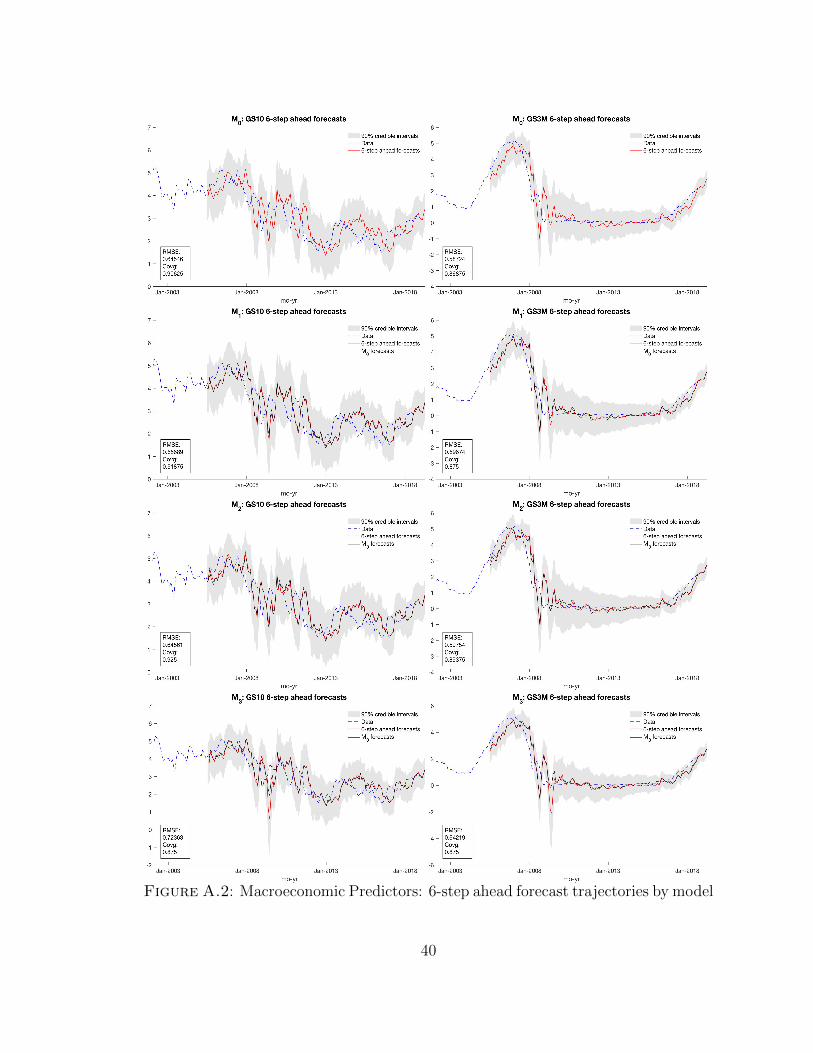
Figure A.2: Macroeconomic Predictors: 6-step ahead forecast trajectories by model

40

Appendix B

DDNM Sample Code

1 %%% Spec i f y model c o v a r i a t e s %%%2 cv t base = data ( : , ’CPI ’ , ’Unemp ’ ) ;3 saveX = double ( cv t base ( 1 3 : end , : ) ) ;4 DD names = [ Yd names , ’CPI ’ , ’Unemp ’ ] ;5

6

7 %%% Model Setup %%%8 Y = cat (1 , saveY ’ , saveX ’ ) ; [ q T]= s i z e (Y) ;9

10 se tddnm yie lds %s e t DDNM s t r u c t u r e11 s e t p r i o r s y i e l d s %p r i o r s & di scount f a c t o r s12

13 % generate k´s tep ahead f o r e c a s t s at t=t f o r e14 k = 12 ;15 index = f i n d ( strcmp ( time , ’Dec´2004 ’ ) ) ;16 t f o r e = index ; % stop FF and f o r e c a s t at t h i s time ;17 l a s t t = max(1 , t f o r e +1´5∗k ) ; % past data to show on p l o t s18 I = 1000 ; %no . o f MC samples f o r each time pt .19

20 %sto rage ar rays21 t i f = T ´ index ;22 s t p rob = ze ro s (1 , t i f ) ; %s t a t i o n a r y prob .23 Cov mat = ze ro s (q , q , t i f , I ) ; %Covariance matrix24 ypred f = ze ro s ( t i f , q , 7 , k ) ; %k´s tep f o r e c a s t summaries25 idx = 0 ;

41

26

27 %%% Training Model and Forecas t ing Resu l t s %%%28

29 f o r t f o r e = index +1:T30 f o r j =1:q % l e a r n i n g phase 1 : t f o r e31 p0 .m=p r i o r 1 , j ; p0 .C=p r i o r 2 , j ∗ p r i o r 4 , j ; p0 . n=

p r i o r 3 , j ; p0 . s=p r i o r 4 , j ;32 p0 . d e l t a=p r i o r 5 , j ; p0 . beta=p r i o r 6 , j ;33 F = ones (1 , t f o r e ) ; i f ( npa ( j )>0) , F=[F ; Y( pa j , 1 :

t f o r e ) ] ; end34 i f ( npr ( j )>0) ,35 f o r h=1: t0 ,36 i=f i n d ( squeeze ( pr ( j , : , h ) ) ) ;37 i f ( l ength ( i )>0) , F = [ F ; [ z e r o s ( l ength ( i ) ,

h ) Y( i , ( h+1: t f o r e )´h) ] ] ; end38 end39 end40 %forward f i l t e r i n g41 pq1t f o r e ( j ) = f f (Y( j , 1 : t f o r e ) ,F , t f o r e , t0 , p0 ) ;42 end43 idx = idx + 1 ; %index f o r f i n a l array s to rage44

45 %f o r e c a s t i n g , s t a r t i n g at t=t f o r e l ook ing ahead46 t = t f o r e ;47 tpred = t f o r e +(1:k ) ; % next k time po in t s48 spred = ze ro s (1 , k , I ) ; % saved s y n t h e t i c f u t u r e s49 ypred = ze ro s (q , 7 , k ) ; % saved f o r e c a s t summaries50 %[ mean , median , SD, 5%, 25%, 75%,

95% ]51

52 k s t e p f o r e c a s t %f o r e c a s t k´s t ep s ahead53

54 %impl i ed VAR companion matrix computation55 st mc = ze ro s (1 , I ) ;56 f o r i =1: I57 id mat = horzcat ( pa mat , reshape ( pr , q , [ ] , 1 ) ) ;58 f o r j =1:q59 s t h e t a j = s the ta j ;60 id mat ( j , f i n d ( id mat ( j , : ) ==1)) = s t h e t a j ( 2 : end , i )

;61 end62

63 Gm = inv ( eye ( q )´id mat ( : , 1 : q ) ) ; Lm = reshape ( id mat

42

( : , q+1:end ) ,q , q , maxlag ) ;64 f o r l =1:maxlag65 Lm( : , : , l ) = Gm∗ squeeze (Lm( : , : , l ) ) ;66 end67 %compute companion matrix68 C mat = v e r t c a t ( reshape (Lm, q , [ ] , 1 ) , horzcat ( eye ( (

maxlag´1)∗q ) , z e r o s (q , ( maxlag´1)∗q ) ) ) ;69 st mc ( i ) = a l l ( abs ( e i g (C mat ) )<1) ;70

71 %compute recoup led cov . matrix72 Cov mat ( : , : , idx , i ) = Gm∗diag ( 1 . / sv ( : , i ) )∗Gm’ ;73 end74 %sto rage ar rays75 s t p rob ( idx ) = mean( st mc ) ; %s t a t i o n a r y prob .76 ypred f ( idx , : , : , : ) = ypred ; %f o r e c a s t summaries77 d i sp l ay ( [ ’ done at time ’ , i n t 2 s t r ( t ) , ’ / ’ , i n t 2 s t r (T) ] )78 end79

80 %log´mlik o f mult iv . 1´s tep pred . dens i ty81 lmk f = sum( v e r t ca t ( pq1t f o r e . lp ) ,1 ) ;82

83

84 %%% k´s tep ahead f o r e c a s t summaries %%%85 id = [ 1 3 6 1 2 ] ;86 rmse dd = ze ro s ( s i z e ( id , 2 ) , 7 ) ;87 covg dd = rmse dd ;88

89 f o r i =1: s i z e ( id , 2 ) %loop over f o r e c a s t hor i zons90 idk = id ( i ) ;91 ypred d = squeeze ( ypred f ( : , : , : , idk ) ) ;92 fm d = squeeze ( ypred d ( : , : , 1 ) ) ’ ; %f o r e c a s t mean93 c i d = ypred d ( : , : , [ 4 end ] ) ; % 90% c r e d i b l e i n t e r v a l s94

95 f o r j =1:7 %loop over each s e r i e s96 rmse = mean ( (Y( j , index+1+idk :T)´fm d ( j , 1 : end´idk ) )

. ˆ 2 ) ;97 rmse dd ( i , j ) = s q r t ( rmse ) ; %s t o r e rmse98 lw = Y( j , index+1+idk :T) >= squeeze ( c i d ( 1 : end´idk , j

, 1 ) ) ’ ;99 upp = Y( j , index+1+idk :T) <= squeeze ( c i d ( 1 : end´idk , j

, 2 ) ) ’ ;100 covg = mean( lw .∗ upp) ;101 covg dd ( i , j ) = covg ; %s t o r e coverage

43

102

103 %produce f i g u r e s104 f i g u r e (9 ) ; c l f ;105 c i p l o t ( squeeze ( c i d ( : , j , 1 ) ) ’ , squeeze ( c i d ( : , j , 2 ) ) ’ ,

index+1+idk :T+idk , [ 0 . 9 0 . 9 0 . 9 ] ) ;106 hold on107 p lo t ( 1 :T,Y( j , : ) , ’ b ’ , index+1+idk :T+idk , fm d ( j , : ) , ’ r ’ )

;108 hold o f f109 t i t l e ( [ char (DD names( j ) ) , ’ : ’ , [ i n t 2 s t r ( idk ) , ’´s tep

ahead f o r e c a s t s ’ ] ] ) ;110 l egend ( ’90% c r e d i b l e i n t e r v a l s ’ , ’ Data ’ , [ i n t 2 s t r ( idk

) , ’´s tep ahead f o r e c a s t s ’ ] , ’ l o c a t i o n ’ , ’ no r theas t ’) ; l egend boxo f f

111 s t r = ’RMSE: ’ , num2str ( s q r t ( rmse ) ) , ’Covg : ’ , num2str( covg ) ;

112 annotat ion ( ’ textbox ’ , [ . 1 5 . 0 . 3 . 3 ] , ’ S t r ing ’ , s t r , ’FitBoxToText ’ , ’ on ’ ) ;

113 eva l ( xa ) ; xl im ( [T´200 T+idk ] ) ;114 pause ;115 end116 end

44

Bibliography

Ang, A. and M. Piazzesi (2003). A no-arbitrage vector autoregression of term struc-ture dynamics with macroeconomic and latent variables. Journal of MonetaryEconomics 50, 745–787.

Ang, A., M. Piazzesi, and M. Wei (2004). What does the yield curve tell us aboutgdp growth? Journal of Econometrics 131, 359–403.

Carriero, A. (2011). Forecasting the yield curve using priors from no-arbitrage affineterm structure models. International Economic Review 52, 425–459.

Chib, S. and B. Ergashev (2009). Analysis of multifactor affine yield curve models.Journal of the American Statistical Association 104, 1324–1337.

Dai, Q. and K. Singleton (2000). Specification analysis of affine term structuremodels. Journal of Finance 55, 1947–1978.

Diebold, F. and C. Li (2006). Forecasting the term structure of government bondyields. Journal of Econometrics 130, 337–364.

Diebold, F., S. Rudebusch, and S. Aruoba (2006). The macroeconomy and the yieldcurve. Journal of Econometrics 131, 309–338.

Duffee, G. (2002). Term premia and interest rate forecasts in affine models. Journalof Finance 57, 405–443.

Duffie, D. and R. Kan (1996). A yield-factor model of interest rates. MathematicalFinance 6, 379–406.

Giannone, D., L. Reichlin, and L. Sala (2004). Monetary policy in real time. NBERMacroeconomics Annual 19, 161–200.

Gruber, L. and M. West (2017). Bayesian forecasting and scalable multivariatevolatility analysis using simultaneous graphical dynamic linear models. Econo-metrics and Statistics 3, 3–22.

Koopman, S., M. Mallee, and M. Van der Wel (2010). Dynamic nelson-siegel modelwith time-varying parameters. Journal of Business & Economic Statistics 28,1324–1337.

45

Moench, E. (2008). Forecasting the yield curve in a data-rich environment: a no-arbitrage factor-augmented var approach. Journal of Econometrics 146, 26–43.

Moench, E. (2012). Term structure surprises: The predictive content of curvature,level, and slope. Journal of Applied Econometrics 27, 574–602.

Nelson, C. and A. Siegel (1987). Parsimonious modeling of yield curves. Journal ofBusiness 60, 473–489.

Prado, R. and M. West (2010). Time Series Modeling, Computation, and Inference.Chapman and Hall/CRC, Taylor and Francis Group.

Zhao, Z., M. Xie, and M. West (2016). Dynamic dependence networks: Financialtime series forecasting & portfolio decisions (with discussion). Applied StochasticModels in Business and Industry 32, 331–339.

46