forecasting with a panel tobit...
TRANSCRIPT

Forecasting with a Panel Tobit Model
Laura Liu
Federal Reserve Board
Hyungsik Roger Moon
University of Southern California
and Yonsei
Frank Schorfheide∗
University of Pennsylvania
CEPR, NBER, and PIER
Preliminary Version: March 4, 2018
Abstract
We use a dynamic panel Tobit model to generate point and density forecasts for
a large cross-section of short time series of censored observations. Our fully Bayesian
approach allows us to flexibly estimate the cross-sectional distribution of heteroge-
neous coefficients and then implicitly use this distribution to construct Bayes forecasts
for the individual time series. We consider versions of the model with homoskedastic
and heteroskedastic innovations. In Monte Carlo experiments and the empirical ap-
plication to loan charge-off rates of small banks, we compare Bayesian point, interval,
and density forecasts obtained from various versions of the panel Tobit model. In our
empirical application the assumption of homoskedasticity yields more accurate point
forecasts, whereas interval and density forecasts are more accurate if computed under
the assumption of heteroskedastic innovations. Local house prices and unemployment
rates do not appear to be significant determinants of charge-off rates.
JEL CLASSIFICATION: C11, C14, C23, C53, G21
KEY WORDS: Bayesian inference, density forecasts, interval forecasts, loan charge-offs,
panel data, point forecasts, Tobit model.
∗Correspondence: L. Liu: Board of Governors of the Federal Reserve System, 20th Street and Con-stitution Avenue N.W., Washington, D.C. 20551. Email: [email protected]. H.R. Moon: Department ofEconomics, University of Southern California, KAP 300, Los Angeles, CA 90089. E-mail: [email protected]. Schorfheide: Department of Economics, 3718 Locust Walk, University of Pennsylvania, Philadelphia, PA19104-6297. Email: [email protected]. Moon and Schorfheide gratefully acknowledge financial supportfrom the National Science Foundation under Grants SES 1625586 and SES 1424843, respectively. The viewsexpressed in this paper are those of the authors and do not necessarily reflect the views of the Board ofGovernors or the Federal Reserve System.

This Version: March 4, 2018 1
1 Introduction
This paper considers the problem of forecasting a large collection of short time series with
censored observations. In particular, in our empirical application we forecast charge-off rates
on loans for a panel of small banks. The prediction of charge-off rates is interesting from a
regulator’s perspective because charge-offs generate losses on loan portfolios. If these charge-
offs are large, the bank may be entering a period of distress and require additional capital.
Due to mergers and acquisitions, changing business models, and changes in regulatory envi-
ronments the time series dimension that is useful for forecasting is often short. The general
methods developed in this paper are not tied to the charge-off rate application and can be
used in any setting in which a researcher would like to analyze a panel of censored data with
a large cross-sectional and a short time series dimension.
The challenge in forecasting short time series is that they do not contain a lot of informa-
tion about unit-specific parameters. An accurate estimation of the heterogeneous coefficients
helps with an accurate forecast. A natural way of adding information is through the use of
prior distributions. For each time series, the prior information can be combined with the
unit-specific likelihood function to form a posterior. From a Bayesian perspective the pos-
terior distribution then can be used to derive a forecast that minimizes posterior expected
loss. From a frequentist perspective one obtains a forecast that will have some bias, but
in a mean-squared-error sense, the introduction of bias might be dominated by a reduction
in sampling variance. The key insight in panel data applications is that in the absence of
any meaningful subjective prior information, one can extract information from the cross
section and equate the prior distribution with the cross-sectional distribution of unit-specific
coefficients.
There are several ways of implementing this basic idea. An empirical Bayes implemen-
tation would create a point estimate of the cross-sectional distribution of the heterogeneous
coefficients and then condition the subsequent posterior calculations on the estimated prior
distribution.1 In fact, the classic James-Stein estimator for a vector of means can be inter-
preted as an estimator constructed as follows. In the first step a prior is generated by fitting
a normal distribution to a cross-section of observations. In a second step, this prior is then
combined with the unit-specific likelihood function to generate a posterior estimate of the
unknown mean for that unit. In a panel setting the implementation is more involved but
1Empirical Bayes methods have a long history in the statistics literature going back to Robbins (1956);see Robert (1994) for a textbook treatment.

This Version: March 4, 2018 2
follows the same steps. If the model is linear in the coefficients and the forecast is evalu-
ated under a quadratic forecast error loss function, then Tweedie’s formula, which expresses
the posterior mean of the heterogeneous coefficients as the maximum likelihood estimate
corrected by a function of the cross-sectional density of sufficient statistic, can be used to
construct a forecast without having to explicitly estimate a prior distribution for the hetero-
geneous coefficients. This insight has been recently used by Brown and Greenshtein (2009),
Gu and Koenker (2016a,b), and Liu, Moon, and Schorfheide (2017).
Unfortunately, Tweedie’s formula does not extend to nonlinear panel data models. Rather
than pursuing an Empirical Bayes strategy, we will engage in a full Bayesian analysis by spec-
ifying a hyperprior for the distribution of heterogeneous coefficients and then constructing
a joint posterior for the coefficients of this hyperprior as well as the actual unit-specific co-
efficients. While the computations are more involved, this approach can in principle handle
quite general nonlinearities. Moreover, it is possible to generate point predictions under
more general loss functions, as well as interval and density forecasts. For a linear panel
data model, a full Bayesian analysis is implemented by Liu (2017). The contribution of our
paper is to extend the implementation to the dynamic panel Tobit model and to apply it
to the problem of forecasting loan charge-off rates. We compare Bayesian point, interval,
and density forecasts obtained from various versions of the panel Tobit model. In our em-
pirical application the assumption of homoskedasticity yields more accurate point forecasts,
whereas interval and density forecasts are more accurate if computed under the assumption
of heteroskedastic innovations. Local house prices and unemployment rates do not appear
to be significant determinants of charge-off rates.
Our paper relates to several branches of the literature. The papers most closely related
are Gu and Koenker (2016a,b), Liu (2017), and Liu, Moon, and Schorfheide (2017). All four
of these papers focus on the estimation of the heterogeneous coefficients in linear panel data
models and the subsequent use of the estimated coefficients for the purpose of prediction.
Only the full Bayesian analysis in Liu (2017) has a natural extension to nonlinear models.
Liu, Moon, and Schorfheide (2017), building on Brown and Greenshtein (2009), show that
an empirical Bayes implementation based on Tweedie’s formula can asymptotically (as the
cross-sectional dimension tends to infinity) lead to forecasts that are as accurate as the so-
called oracle forecasts. Here an oracle forecast is an infeasible benchmark that assumes that
all homogeneous coefficients, as well as the distribution of the heterogeneous coefficients, are
known to the forecaster. Liu (2017) shows that the predictive density obtained from the full
Bayesian analysis converges strongly to the oracle’s predictive density as the cross-section

This Version: March 4, 2018 3
gets large.
There is a Bayesian literature on the estimation of censored regression models. The idea
of using data augmentation and Gibbs sampling to estimate a Tobit model dates back to
Chib (1992). To sample the latent uncensored observations we rely on an algorithm tailored
toward dynamic Tobit models by Wei (1999). Sampling from truncated normal distributions
is implemented with a recent algorithm of Botev (2017). A broader survey of the literature
on Bayesian estimation of univariate and multivariate censored regression models can be
found in the handbook chapter by Li and Tobias (2011).
We consider two approaches of modeling the unknown distribution of the heterogeneous
coefficients. First, we assume that this distribution belongs to the class of Normal distribu-
tions (or Normal and Inverse Gamma if we allow for heteroskedasticity). Second, we consider
a more flexible setup in which the distribution is represented by Dirichlet process mixtures
of Normals. Even though we do not emphasize the nonparametric aspect of this modeling
approach (due to a truncation, our mixtures are strictly speaking finite and in that sense
parametric), our paper is related to the literature on flexible / nonparametric density mod-
eling using Dirichlet process mixtures (DPM). Examples of papers that use DPMs in the
panel data context are Hirano (2002), Burda and Harding (2013), Rossi (2014), and Jensen,
Fisher, and Tkac (2015). The implementation of our Gibbs sampler relies on Ishwaran and
James (2001, 2002).
Our analysis raises the question to what extent the cross-sectional distribution of the
heterogeneous coefficients is identifiable. Even though identification is not a necessary pre-
requisite for a Bayesian analysis as discussed, for instance in Moon and Schorfheide (2012)
and references cited therein, it is important to understand in what directions of the parameter
space one can expect to learn from the data. There exists a large literature on identification
in nonlinear panel data models. Earlier censored panel regression analysis mostly focused on
the established identification and estimating the homogeneous regression coefficients under
fixed effects. Examples of these studies include Honore (1992) (static model), Hu (2002) (dy-
namic model), and Abrevaya (2000) (generalized fixed effect model), Honore and Hu (2004)
(endogenous censored panel regression), and Arellano and Honore (2001) (survey on panel
Tobit type regressions).
More recent papers investigated more general nonlinear and non-separable panel regres-
sion models. Here the conventional censored panel regression is a special case and the
literature established identification of various parameters of interests such as regression co-

This Version: March 4, 2018 4
efficients, marginal effects, average structural function, and average treatment effects (e.g.,
Bester and Hansen (2009), Altonji and Matzkin (2005), Bonhomme (2012), and Hoderlein
and White (2012). The paper most relevant to our analysis is that of Hu and Shiu (2018).
They obtain identification results for censored dynamic panel data models with parametric
specifications of the dynamics, censoring, and distribution of the shocks, but a nonpara-
metric specification of the distribution of the unobserved individual effects. This covers the
benchmark model considered in Section 2.
The remainder of this paper is organized as follows. The basic dynamic panel Tobit
model with homoskedastic shocks is presented in Section 2. We discuss its specification and
develop a sampler for posterior inference. This model is extended to allow for cross-sectional
heteroskedasticity in Section 3 and further generalizations are sketched out in Section 4. We
conduct a Monte Carlo experiment in Section 5 to examine the performance of the proposed
techniques in a controlled environment. An empirical application in which we forecast charge-
off rates on various types of loans for a panel of banks is presented in Section 6. Finally,
Section 7 concludes. A description of the data sets, additional empirical results, and some
derivations are relegated to the Online Appendix.
2 The Basic Model
To fix ideas, we consider the following dynamic panel Tobit model with heterogeneous inter-
cepts:
yit = yit∗I{y∗it ≥ 0}, i = 1, . . . , N, t = 0, . . . , T (1)
y∗it = λi + ρy∗
it−1 + uit, uitiid∼ N(0, σ2), y∗
i,0 ∼ N(μi∗, σ2∗),
where I{x ≥ a} is the indicator function that is equal to one if x ≥ a and equal to zero
otherwise. Let θ = [ρ, σ2]′. The parameters that characterize the distribution of y∗i,0 could
either be a function of (θ, λi), e.g., μi∗ = λi/(1 − ρ) and σ2∗ = σ2/(1 − ρ2) or they could
be fixed, e.g., μi∗ = 0 and σ2∗ = 0. We assume that conditional on the parameters the
observations are cross-sectionally independent and that the heterogeneous intercepts λi are
distributed according to an unknown random effects distribution
λiiid∼ π(λ). (2)

This Version: March 4, 2018 5
The density π(∙) can be viewed as an unknown, possibly infinite-dimensional parameter. Our
goal is to generate forecasts of yiT+h conditional on the observations
Y1:N,0:T ={(y10, . . . , yN0), . . . , (y1T , . . . , yNT )
}.
A natural benchmark against which we can compare our forecasts is the so-called oracle
forecast that is obtained under the assumption that θ and π(∙) are known but λi is unknown.
Due to the cross-sectional independence, the oracle forecast can be derived from the posterior
predictive distribution of yiT+h given(Yi,0:T , θ, π(∙)
). Define the posterior distribution of λi
as
p(λi|Yi,0:T , θ, π) ∝ p(Yi,1:T |yi,0, θ, λi)π(λi), (3)
where p(Yi,1:T |yi,0, θ, λi) is the conditional likelihood function associated with (1). Then, the
posterior predictive distribution is given by
p(yiT+h|Yi,0:T , θ, π) (4)
=
∫p(yiT+h|y
∗iT+h)p(y∗
iT+h|y∗iT , θ, λi)p(y∗
iT |Yi,0:T , θ, λi)p(λi|Yi,0:T , θ, π)dy∗iT dλi.
The distribution of yiT+h|y∗iT+h is a unit point mass that is located at zero if y∗
iT+h ≤ 0 or at
y∗iT+h if y∗
iT+h > 0. The density p(y∗iT+h|y
∗iT , θ, λi) is generated by the forward simulation of
the autoregressive law of motion for y∗it in (1) and the remaining two densities are posteriors
for y∗iT and λi. In Section 2.1 we discuss the computation of the oracle predictor. Sections 2.2
and 2.3 focus on the estimation of θ and π, respectively. With the exception of the treatment
of the latent variables Y ∗i,0:T , the computations for the Tobit model are very similar to the
ones for the linear model studied in Liu (2017).
2.1 Oracle Forecast
In order to implement the oracle forecasts we will use a data augmentation algorithm (see
Tanner and Wong (1987)) to generate draws from the posterior predictive distribution in
(??). The implementation of this algorithm is based on Wei (1999) who studied the Bayesian
estimation of univariate dynamic Tobit models. For each unit i, the data augmentation
algorithm iterates over the following two conditional posteriors:
Y ∗i,0:T |(Yi,0:T , θ, λi) and λi|(Yi,0:T , Y ∗
i,0:T , θ, π), (5)

This Version: March 4, 2018 6
thereby generating draws from the joint distribution of (Y ∗i,0:T , λi)|(Yi,0:T , Y ∗
i,0:T , θ, π) that can
be used to approximate the oracle predictor in equation (4).
Drawing from Y ∗i,0:T |(Yi,0:T , θ, λi). To fix ideas, consider the following sequence of observa-
tions yi0, . . . , yiT :
y∗i0, y∗
i1, 0, 0, 0, y∗i5, y∗
i6, 0, 0, 0, y∗i10.
Our model implies that whenever yit > 0 we can deduce that y∗it = yit. Thus, we can
focus our attention on periods in which yit = 0. In the hypothetical sample we observe
two strings of censored observations: (yi2, yi3, yi4) and (yi7, yi8, yi9). We use t1 for the start
date of a string of censored observations and t2 for the end date. In the example we have
two such strings, we write t(1)1 = 2, t
(1)2 = 4, t
(2)1 = 7, t
(2)2 = 9. The goal is to characterize
p(Y ∗i,t
(1)1 :t
(1)2
, Y ∗i,t
(2)1 :t
(2)2
|Yi,0:T , θ, λi). Because of the AR(1) structure, observations in periods
t < t1 − 1 and t > t2 + 1 contain no additional information about y∗it1
, . . . , y∗it2
. Thus, we
obtain
p(Y ∗i,t
(1)1 :t
(1)2
, Y ∗i,t
(2)1 :t
(2)2
|Yi,0:T , θ, λi)
= p(Y ∗i,t
(1)1 :t
(1)2
|Yi,t
(1)1 −1:t
(1)2 +1
, θ, λi)p(Y ∗i,t
(2)1 :t
(2)2
|Yi,t
(2)1 −1:t
(2)2 +1
, θ, λi),
which implies that we can sample each string of latent observations independently.
Let s = t2 − t1 + 2 be the length of the segment that includes the string of censored
observations as well as the adjacent uncensored observations. Iterating the AR(1) law of
motion for yit forward from period t = t1 − 1 we deduce that the vector of random variables
[Y ∗i,t1:t2
, yit2+1]′ conditional on yit1−1 is multivariate normal with mean
M1:s|0 = [μ1, . . . , μs]′, μ1 = λ + ρyit1−1, μτ = λ + ρμτ−1 for τ = 2, . . . , s. (6)
The covariance matrix takes the form
Σ1:s|0 = σ2
ρ1,1|0 ∙ ∙ ∙ ρ1,s|0...
. . ....
ρs,1|0 ∙ ∙ ∙ ρs,s|0
, ρi,j|0 = ρj,i|0 = ρj−i
i−1∑
l=0
ρ2l for j ≥ i. (7)
We can now use the formula for the conditional mean and variance of a multivariate normal

This Version: March 4, 2018 7
distribution
M1:s−1|0,s = M1:s−1|0 − Σ1:s−1,s|0Σ−1ss|0(yit2+1 − μs) (8)
Σ1:s−1,1:s−1|0,s = Σ1:s−1,1:s−1|0 − Σ1:s−1,s|0Σ−1ss|0Σs,1:s−1|0
to deduce that
Y ∗i,t1:t2
∼ TN−
(M1:s−1|0,s, Σ1:s−1,1:s−1|0,s
). (9)
Here we use TN−(μ, Σ) to denote a normal distribution that is truncated to satisfy y ≤
0. Draws from this truncated normal distribution can be efficiently generated using the
algorithm recently proposed by Botev (2017).
There are two important special cases. First, suppose that t2 = T , meaning that the
last observation in the sample is censored. Then the mean vector and the covariance matrix
of the truncated normal distribution are given by (6) and (7) with the understanding that
s = t2 − t1 + 1. Second, suppose that t1 = 0, meaning that the initial observation in the
sample yi0 = 0. Because in this case the observation yit1−1 = yi,−1 is missing, we need to
modify the expressions in (6) and (7). According to (1), y∗0 ∼ N(μ∗, σ
2∗). This leads to the
mean vector
M1:s = [μ1, . . . , μs], μ1 = μ∗, μτ = λ + ρμτ−1 for τ = 2, . . . , s. (10)
and the covariance matrix
Σ1:s = σ2
0 0 ∙ ∙ ∙ 0
0 ρ1,1 ∙ ∙ ∙ ρ1,s−1
......
. . ....
0 ρs−1,1 ∙ ∙ ∙ ρs−1,s−1
+ σ2∗
ρ0+0 ∙ ∙ ∙ ρ0+(s−1)
.... . .
...
ρ(s−1)+0 ∙ ∙ ∙ ρ(s−1)+(s−1)
, (11)
where the definition of ρi,j is identical to the definition of ρi,j|0 in (7). One can then use
the formulas in (8) to obtain the mean and covariance parameters of the truncated normal
distribution.
Drawing from λi|(Yi,0:T , Y ∗i,0:T , θ, π). The posterior inference with respect to λi becomes
“standard” once we condition on the latent variables Y ∗i,0:T . It is based on the Gaussian
location-shift model
y∗it − ρy∗
it−1 = λi + uit, uitiid∼ N(0, σ2). (12)

This Version: March 4, 2018 8
If the prior distribution π(λ) is Gaussian, the posterior of λ will be Gaussian and direct
sampling from λi|(Yi,0:T , Y ∗i,0:T , θ, π) is straightforward. If π(λ) is non-Gaussian, a draw could
be generated with a Metropolis-Hastings (MH) step.
Drawing from the predictive density. Conditional on (y∗iT , θ, λi) the predictive distri-
bution of yiT+h is given by a censored (at zero) normal distribution (CN+):
yiT+h|(y∗iT , θ, λi) ∼ CN+
(
λi
h−1∑
l=0
ρl + ρhy∗iT , σ2
h−1∑
l=0
ρ2l
)
. (13)
Draws from this distribution can be generated by direct sampling and analytical formula for
the mean and the variance are available (see Greene (2008) and the Online Appendix).
2.2 Estimating θ
We now consider the conditional posterior distribution θ|(Yi,0:T , Y ∗i,0:T , λi, π). Note that con-
ditional on the latent observations Y ∗i,0:T the actual observations Yi,0:T contain no additional
information. Moreover, conditional on λi the density π(λ) is irrelevant for inference on θ.
We can rewrite the law-of-motion for y∗it as
y∗it − λi = ρy∗
it−1 + uit, uitiid∼ N(0, σ2), i = 1, . . . , N and t = 1, . . . , T. (14)
Conditional on the λi’s we have a Gaussian linear regression model with unknown slope
coefficient ρ and unknown variance σ2. The temporal and spatial independence of the uit’s
allows us to pool observations across i and t. If we use a conjugate Normal-Inverse-Gamma
(NIG) prior, then the conditional posterior θ|(Y ∗i,0:T , λi) also belongs to the NIG family.
2.3 Estimating π(λ)
To model the unknown random effects distribution π(λ) we consider a tightly parameterized
approach under which π(λ) is assumed to be Gaussian with unknown scale and location
parameter and a more flexible approach in which we use a Dirichlet Process Mixture (DPM)
to generate a prior distribution for π(λ).
Parametric treatment of π(λ). We assume that π belongs to the family of normal
distributions and write pN (x|μ, σ2) to denote the density of a N(μ, σ2). Using this notation,

This Version: March 4, 2018 9
let
p(λ|π) = pN
(λ|μλ, ω
2λ
). (15)
Thus, here the distribution π(λ) is represented by the two-dimensional parameter vector
[μλ, ω2λ]
′. To induce a prior distribution for the hyperparameters (μλ, ω2λ) we assume that
p(ω2
λ
)= pIG
(ω2
λ
∣∣2, 2), p
(μλ|ω
2λ
)= pN
(μλ|0, ω
2λ
), (16)
where pIG(x|a, b) is the density of an Inverse Gamma IG(2, 2) distribution.
Recall from (12) that the likelihood function for λi obtained from the latent variables
Y ∗i,0:T is Gaussian. Thus, we deduce that the conditional posterior distribution
p(λi|Yi,0:T , Y ∗i,0:T , θ, π) ∝ p(Yi,0:T |Y
∗i,0:T )p(Y ∗
i,0:T |λi, θ)p(λi|π) (17)
is also Normal. The conditional posterior distribution for the parameters of the random-
effects distribution can be characterized as follows:
p(μλ, ω2λ|Y1:N,0:T , Y ∗
1:N,0:T , λ1:N , θ) ∝ p(μλ, ω2λ)
N∏
i=1
p(λi|μλ, ω2λ). (18)
Here the densities p(Y ∗i,0:T |λi, θ) are absorbed in the constant of proportionality because they
do not depend on (μλ, ω2λ).
Flexible treatment of π(λ). For a nonparametric treatment of π(λ) we are essentially
replacing the Gaussian density in (15) with a mixture of normals. This implies that in
addition to specifying priors for the means and variances of the normal distributions as in
(16), we need to specify the number of mixture components and probabilities associated with
the mixture components. This leads to a truncated stick breaking (TSB) representation of
a DPM prior.
We fix the maximum number of mixture components of π(λ) at a large number K.2
Each component k, k = 1, . . . , K corresponds to a N(μk, ω2k) distribution. The probability
assigned to component k is denoted by πk and normalized such that∑K
k=1 πk = 1. Then,
p(λ|π) =K∑
k=1
πkpN
(λ|μk, ω
2k
). (19)
2In our simulations we choose K = 20. This leads to the following uniform bound on the approximationerror (see Theorem 2 of Ishwaran and James (2001)): ‖fλ,K − fλ‖ ∼ 4N exp[−(K − 1)/α] ≤ 2.24× 10⁻⁵, atthe prior mean of α (α = 1) and a cross-sectional sample size N = 1000.

This Version: March 4, 2018 10
To induce a prior distribution over the random effects distribution, we need priors for the
means and variances of the mixture components, extending (16) above:
p(ω2
k
)= pIG
(ω2
k
∣∣2, 2), p
(μk|ω
2k
)= pN
(μk|0, ω
2k
), k = 1, . . . , K. (20)
The prior for the mixture probabilities πk is generated by a TSB(1, α,K) process of the
form
πk|(α,K) ∼
ζ1, k = 1,∏k−1
j=1 (1 − ζj) ζk, k = 2, . . . , K − 1,
1 −∑K−1
j=1 pj , k = K,
, ζk ∼ B(1, α) (21)
where B(α, β) is the Beta distribution. Finally, we use an IG prior for the hyperparameter
α of the TSB:
p(α) = pIG(α|2, 2). (22)
In order to characterize the posterior distribution, we introduce some additional notation.
Because π(λ) is a mixture, ex post, each λi is associated with one of the K mixture compo-
nents. Let γi ∈ {1, . . . , K} be the component affiliation of unit i. Moreover, let nk be the
number of units and Jk the set of units affiliated with component k. Using the component
indicator γi we can rewrite (17) as
p(λi|Yi,0:T , Y ∗i,0:T , θ, π, γi) ∝ p(Yi,0:T |Y
∗i,0:T )p(Y ∗
i,0:T |λi, θ)
[K∑
k=1
I{γi = k}pN(λi|μk, ω2k)
]
, (23)
where I{γi = k} is the indicator function that is one if γi = k and zero otherwise. Thus,
conditional on γi the posterior of λi remains Normal. The analogue of (18) becomes:
p(μk, ω2k|Y1:N,0:T , Y ∗
1:N,0:T , λ1:N , θ) ∝ p(μk, ω2k)∏
i∈Jk
p(λi|μk, ω2k). (24)
The prior probability that unit i is affiliated with component k is given by πk. Let πik
denote the posterior probability conditional on the set of means μ1:k and variances ω21:K as
well as λi. The πik’s are given by
πik =πkpN
(λi|μk, ω
2k
)
∑Kk=1 πkpN
(λi|μk, ω2
k
) . (25)

This Version: March 4, 2018 11
Thus,
γi|(μ1:k, ω21:K , λi) = k with prob. πik. (26)
Based on γ1:N one can determine nk and Jk for k = 1, . . . , N . The conditional posterior of
the component probabilities takes the form
πk|(n1:K , α,K) ∼ TSB
(
1 + nk, α +∑
j=k+1
nj , K
)
, (27)
meaning that the ζk’s in (21) have a B(1 + nk, α +
∑j=k+1 nj
)distribution. Conditional on
π1:K the hyperparameter α has a Gamma (G) posterior distribution of the form
α|π1:K ∼ G(2 + K − 1, 2 − ln πK). (28)
Gibbs Sampling. A Gibbs sampler can be obtained by sampling from the various con-
ditional posterior distributions above. The sampler for the flexible mixture representation
of π(λ) is based on Ishwaran and James (2001, 2002). The Gibbs sampler iterates over the
following posterior distributions: the latent variables Y ∗i,0:T in (9), the homogeneous param-
eters θ in Section 2.2, the heterogeneous parameters λi in (23), the scale parameter α of
the Dirichlet distribution in (28), the mixture weights πk in (27), the mixture component
parameters (μk, ω2k) in (24), and the mixture component memberships γi in (26). The Gibbs
sampler for the model with Gaussian π(λ) omits the steps to draw α, πk, and γi. Moreover,
it only has to generate a single pair (μ, ω2).
3 A Model With Heteroskedasticity
In the benchmark model (1) we assumed that the innovations uit are homoskedastic. We
now generalize this assumption to allow for heteroskedasticity:
uitiid∼ N(0, σ2
i ). (29)
Now σ2i is an additional heterogeneous parameter. We will specify a prior distribution
according to which λi and σ2i are independent of each other, i.e., π(λ, σ2) = π(λ)π(σ2). We
consider a parametric treatment of π(σ2) that can be combined with the Gaussian prior for
λ and a more flexible class of priors for σ2 that we combine with the mixture prior for λ.

This Version: March 4, 2018 12
Parametric treatment of π(σ2). Here we assume that π(σ2) belongs to the Inverse Gamma
(IG) family and is indexed by the hyperparameters a and b: pIG(σ2|a, b). In specifying the
prior for the hyperparameters, we follow Llera and Beckmann (2016) and let
b ∼ G(αb, βb), p(a|b) ∝
α−(1+a)a baγ
a
Γ(a)βa
. (30)
The parameters (αa, βa, γ
a, αb, βb
) need to be chosen by the researcher. We use αa = 1, βa
=
γa
= αb = βb
= 0.01, which specifies relatively uninformative priors for hyperparameters a
and b. Suppose we have a sequence of observations σ2i , i = 1, . . . , N . Then the joint posterior
for (a, b) takes the form
p(a, b|σ21:N ) ∝ pIG(σ2|a, b)pG(ab0, bb0)p(a|b) (31)
∝
(ba
Γ(a)
)N(
N∏
i=1
(σ2
i
)−(a+1)
)
exp
{
−bN∑
i=1
1/σ2i
}
×bαb−1 exp{−β
bb} α
−(1+a)a baγ
a
Γ(a)βa
Thus, the conditional posterior of b|a takes the form of a Gamma G(αb, βb) distribution
with parameters αb = αb + Na and βb = βb+∑N
i=1 1/σ2i . The conditional posterior of a|b
has the same kernel as the prior with parameters ln αa = ln αa +∑N
i=1 ln σ2i , βa = β
a+ N ,
and γa = γa
+ N . Because it is not possible to directly sample from this distribution, we
use a Metropolis-within-Gibbs sampler with a random-walk proposal density to draw from
p(a, b|σ21:N).3 Conditional on the hyperparameters (a, b) it is straightforward to generate
draws from the posterior of σ2i by directly sampling from the appropriate Inverse Gamma
distributions.
Flexible treatment of π(σ2). We use the same approach as for π(λ), described in Sec-
tion 2.3. A DPM of normal distributions is used to generate a prior for ln σ2. The conditional
posteriors of hyperparameters are essentially identical to the ones that arose in the context of
π(λ). Given mixture component k, the conditional posterior distribution of σ2i is proportional
to
p(σ2i |∙) ∝ (σ2
i )−1pN(ln σ2
i |μσ2,k, ωσ2, k)
T∏
t=1
pN (yit|ρy∗it−1 + λi, σ
2i ). (32)
We sample from this non-standard posterior via an adaptive random walk Metropolis-
3We use an adaptive procedure based on Atchade and Rosenthal (2005) and Griffin (2016), which adap-tively adjusts the random walk step size to keep acceptance rates around 30%.

This Version: March 4, 2018 13
Hastings (RWMH) step.
4 Generalizations
The basic dynamic panel Tobit model given by (1) and (29) can be generalized in several
dimensions. First, one can include additional covariates with a homogeneous coefficient,
which increases the dimension of the vector θ. This is done in the empirical analysis in
Section 6; see (34). Second, it is fairly straightforward to allow for randomly missing ob-
servations by modifying the inference about the latent variables yit∗ in Section 2.1. Rather
than drawing the latent variables in the data-augmentation algorithm from a truncated nor-
mal distribution, we need to draw them from a regular normal distribution. Third, we can
allow for correlated random effects by replacing the unconditional distribution π(λ) with a
conditional distribution π(λ). Liu (2017) discusses both the Normal as well as the flexible
implementation of a correlated random effects specification. It requires an adjustment to
the prior distribution of the λi’s and an adjustment in the part of the Gibbs sampler that
generates draws from the hyperparameters that index the random effects distribution.
Fourth, the panel setup can be extended to richer limited-dependent variable models.
Let Yit = [y1,it, . . . , yK,it]′ and Y ∗
it = [y∗1,it, . . . , y
∗K,it]
′ and consider
yit = m(Y ∗it ), Y ∗
it |(Y∗it−1, λi, θ) ∼ pY ∗
it |(Y∗it−1, λi, θ), (λi, Y
∗i0)|θ ∼ π(λi, Y
∗i0|θ), (33)
where m(∙) is a known function, p(∙) is a known homogeneous transition density for Y ∗it ,
and π(∙) is the correlated random-effects distribution. In the benchmark model (1) the
dependent variable is a scalar, i.e., K = 1, the transformation of the latent variable is given
by m(y∗it) = y∗
itI{y∗it ≥ 0}, and the transition density is N(λi + ρy∗
it, σ2). In addition to this
standard Tobit model, Amemiya (1985) defines four generalizations. For instance, in the
so-called Type 2 Tobit model K = 2 and the m(∙) function takes the form
m(∙) : y1,it = I{y∗1,it ≥ 0}, y2,it = y∗
2,itI{y∗1,it ≥ 0},
in which the censoring of observation y2,it depends on the observed sign of the latent vari-
able y∗1,it. In order to implement richer Tobit models in our dynamic panel framework one
has to modify the sampler for the conditional posterior distribution of the latent variables
Y ∗i,0:T |(Yi,0:T , λi, θ) described in Section 2.1. For instance, a posterior sampler for the (static)

This Version: March 4, 2018 14
Type 2 Tobit model is discussed in Li and Tobias (2011). The current version of this paper
does not spell out any of these generalizations in detail, except that we allow for additional
covariates in our empirical application.
5 Monte Carlo Experiment
The Monte Carlo experiment is based on the basic dynamic panel Tobit model in (1). The
design of the experiment is summarized in Table 1. We set the autocorrelation parameter
to ρ = 0.8 and normalize the innovation variance of the uit’s to σ2 = 1. We consider
four distributions for the heterogeneous intercept λi: a normal distribution as well as three
mixtures of normals that exhibit skewness, kurtosis, and bi-modality, respectively. The
distributions are parameterized such that E[λi] = 1/2 and V[λi] = 1. The simulated panel
data sets consist of N = 1, 000 cross-sectional units and the number of time periods in the
estimation sample is T = 10. We generate one-step-ahead forecasts for period t = T + 1.
Measures of forecast accuracy are computed as follows. For the evaluation of point
forecasts (and estimators) based on forecast (estimation) error statistics (i.e, RMSE, bias,
and standard deviation), we pool all forecast errors across i = 1, . . . , N = 1, 000 and across
the nsim = 100 Monte Carlo samples Y1:N,1:T+1, which means we are averaging across 105
errors. For the evaluation of interval forecasts, density forecasts, and the probability of
YiT+1 = 0, we compute the performance statistic based on the cross-section i = 1, . . . , N =
1, 000 and then average the performance statistics over the nsim Monte Carlo samples.4
We will compare the performance of six predictors described below: the oracle predictor,
Bayes predictors derived from three versions of the dynamic panel Tobit model that differ
in terms of the treatment of π(λ), and predictors derived from pooled Tobit and pooled
linear models. The prior distributions used for the estimation of the underlying models are
summarized in Table 2.
Oracle Forecast. The oracle knows the parameters θ = (ρ, σ2) as well as the random effects
distribution π(λ). However, the oracle does not know the specific λi values.
Posterior Predictive Distributions Based on Dynamic Panel Tobit Model. We
construct posterior predictive distributions for the dynamic Tobit panel data model under
the following assumptions on π(λ): (i) π(λ) is Gaussian; see (15). (ii) π(λ) is a mixture of
4If the performance statistic is linear, e.g., the coverage probability or the average length of credible sets,then averaging the statistic is the same as pooling across i and across Monte Carlo samples.

This Version: March 4, 2018 15
Table 1: Monte Carlo Design 1
Law of Motion: y∗it = λi + ρy∗
it−1 + uit where uitiid∼ N(0, σ2). ρ = 0.8, σ2 = 1
Initial Observations: y∗i0 ∼ N(0, 1)
Random Effects Distributions:(a) Normal: π(λi|Yi0) = pN
(λi|12 , 1
)
(b) Skewed: π(λi|Yi0) = 19pN
(λi|52 ,
12
)+ 8
9pN
(λi|14 ,
12
)
(c) Fat Tailed: π(λi|Yi0) = 45pN
(λi|12 ,
14
)+ 1
5pN
(λi|12 , 4
)
(d) Bimodal: π(λi|Yi0) = 0.35 ∙ pN
(λi|0, 1
)+ 0.65 ∙ pN
(λi|10, 1
), λi = 1
2+ (λi − E[λi])/
√V[λi]
Sample Size: N = 1, 000, T = 10Number of Monte Carlo Repetitions: Nsim = 100Fraction of zeros: (a) 31%, (b) 32%, (c) 21%, (d) 35%
normal distributions; see (19). (iii) The posterior for each unit i is computed based on the
improper prior λ ∼ U [−9.5, 10.5]. Thus, for this predictor, we do not use any cross-sectional
information to make inference about π(λ).
Pooled Tobit. This specification ignores the heterogeneity in λi, sets λi = λ for all i,
and treats λ as another homogeneous parameter, just like (ρ, σ2). Posterior sampling is
implemented by iteratively sampling from Y ∗i,0:T |(Yi,0:T , λ, ρ, σ2) as described in Section 2.1
and from the distribution of (λ, ρ, σ2)|Y ∗i,0:T as discussed in Section 2.2. Point, interval,
and density forecasts are obtained by generating draws y∗iT+h from the posterior predictive
distribution and then applying the censoring yiT+h = y∗iT+hI{y
∗iT+h ≥ 0}.
Pooled Linear. This specification imposes heterogeneity of the λi’s, i.e., λi = λ for all i,
and, in addition, ignores the censoring of the observations, i.e., assumes yit = y∗it. Because in
the absence of the censoring the model is linear, the posterior of (ρ, σ2, λ) belongs to the NIG
family and sampling is straightforward. To generate point, interval, and density forecasts,
we simulate trajectories from the posterior predictive distribution and apply the censoring
yiT+h = y∗iT+hI{y
∗iT+h ≥ 0} ex post.
Implementation Details. The estimators of the Tobit models are based on the initial
distribution y∗i0 ∼ N(0, σ2). The Gibbs sampler for the model specification with flexible π(λ)
is initialized as follows: y∗1:N,0:T with y1:N,0:T ; (ρ, σ2) with GMM(AB); λi with 1
T
∑Tt=1(y
∗it −
ρy∗it−1); α with its prior mean; γi with k-means with 10 clusters; (μk, ω
2k, πk) are drawn
from the conditional posteriors described in Section 2.3. The Gibbs samplers for the other
specifications are special cases in which some of the parameter blocks drop out. We generate
a total of M0 +M = 10, 000 draws using the Gibbs sampler and discard the first M0 = 1, 000

This Version: March 4, 2018 16
Table 2: Summary of Prior Distributions
Specification λ π(λ)Normal π(λ) λ ∼ N(μλ, ω
2λ) ω2
λ ∼ IG(2, 2), μλ|ω2λ ∼ N(0, ω2
λ)
Flexible π(λ) λ ∼∑K
k=1 πkN(μk, ω2k) ω2
k ∼ IG(2, 2), μk|ω2k ∼ N(0, ω2
k)πk ∼ TSB(1, α,K), α ∼ IG(2, 2)
Flat π(λ) λ ∼ U [−9.5, 10.5]
Pooled Tobit λ ∼ N(0, σ2)
Pooled Linear λ ∼ N(0, σ2)Prior for θ σ2 ∼ IG(2, 2), ρ|σ2 ∼ N(0, σ2)Heteroskedasticity σ2
i ∼ IG(a, b), prior for hyperparameters is given by (30)(Parametric π(σ2)) with αa = 1, β
a= γ
a= αb = β
b= 0.01.
Heteroskedasticity ln σ2i ∼
∑Kk=1 πkN(μk, ω
2k), where
(Flexible π(σ2)) ω2k ∼ IG(2, 2), μk|ω2
k ∼ N(0, ω2k), πk ∼ TSB(1, α,K), α ∼ IG(2, 2).
draws.
Point Forecasts and Parameter Estimates. In 3 we report root-mean-squared errors
(RMSEs) for posterior mean point forecasts. We decompose the RMSEs into a bias and stan-
dard deviation component. We also report the average point estimates of ρ and σ2 across
the repetitions of the Monte Carlo experiment. The results for the oracle serve as a bench-
mark. For all four DGPs the predictors obtained under the flat prior for λ are dominated
by the predictors that estimate π(λ) from the cross-sectional distribution. Modeling π(λ)
as Gaussian distribution works well under Gaussian, skewed, and fat-tailed random effects.
For the bi-modal random effects DGP, the predictor obtained by approximating π(λ) with a
mixture of normals dominates the Gaussian predictor. The pooled linear specification per-
forms significantly worse than all competitors because it ignores the censoring which leads
to a large bias. For all but the pooled linear estimator and, in some instances the predictor
obtained under a flat prior for λ, the bias component of the RMSE is negligible.
Each model delivers a forecast of the probability that yiT+1 = 0. We use this probability
as a point forecast of I{yiT+1 = 0} and compute the corresponding RMSEs, which are also
reported in 3. The RMSE differential between the first five model specifications is negligible.
The predictor derived from the pooled linear model performs significantly worse than the
other predictors in all four Monte Carlo designs. We also computed RMSEs for a perfect
predictor that is constructed based on knowing each (λi, y∗iT ) in addition to θ. The values

This Version: March 4, 2018 17
Table 3: Monte Carlo Experiment: Point Forecast Performance
Forecast Error Stats θ EstimatesRMSE Bias StdD RMSE I{yiT+1 = 0} Bias(ρ) Bias(σ2)
(a) Gaussian Random EffectsOracle 0.85 .004 0.85 0.22 N/A N/ANormal π(λ), estimated θ 0.85 .004 0.85 0.22 0 0Flexible π(λ), estimated θ 0.85 .003 0.85 0.22 0 0Flat π(λ), estimated θ 0.85 0.07 0.85 0.22 -0.08 0Pooled Tobit 0.88 -0.18 0.86 0.22 0.22 0.37Pooled Linear 0.93 -0.32 0.87 0.36 0.21 -0.15
(b) Skewed Random EffectsOracle 0.83 .005 0.83 0.25 N/A N/ANormal π(λ), estimated θ 0.83 -0.01 0.83 0.24 0 0.01Flexible π(λ), estimated θ 0.83 -0.01 0.83 0.24 0.01 0.01Flat π(λ), estimated θ 0.84 0.05 0.84 0.25 -0.08 0.01Pooled Tobit 0.88 -0.19 0.85 0.25 0.23 0.42Pooled Linear 0.92 -0.34 0.85 0.37 0.22 -0.13
(c) Fat-tailed Random EffectsOracle 0.89 0.02 0.89 0.24 N/A N/ANormal π(λ), estimated θ 0.89 -0.01 0.89 0.24 0 0.01Flexible π(λ), estimated θ 0.89 -0.02 0.89 0.24 0.01 0.02Flat π(λ), estimated θ 0.89 0.07 0.89 0.24 -0.09 0Pooled Tobit 0.92 -0.19 0.90 0.24 0.21 0.34Pooled Linear 0.95 -0.30 0.90 0.33 0.21 -0.09
(d) Bi-modal Random EffectsOracle 0.82 .004 0.82 0.08 N/A N/ANormal π(λ), estimated θ 0.84 0.03 0.84 0.09 0 -0.02Flexible π(λ), estimated θ 0.82 0.02 0.82 0.08 -0.01 -0.01Flat π(λ), estimated θ 0.85 0.09 0.85 0.09 -0.07 -0.01Pooled Tobit 0.88 -0.15 0.86 0.10 0.22 0.35Pooled Linear 0.92 -0.29 0.88 0.38 0.18 0.17
Notes: The design of the experiment is summarized in 1. The true values for ρ and σ2 are 0.8 and 1.0,respectively.
are 0.20, 0.23, 0.23, and 0.08, respectively, and thus slightly smaller than the oracle which
only knows π(λ) but not (λi, y∗iT ) for each unit.5
Finally, the last two columns of 3 show the means of the Bayes estimators of ρ and σ2.
5If Y ∈ {0, 1} and the probability of Y = 0 is p, then the RMSE associated with the optimal forecastI{Y = 0} = 1 − p is
√p(1 − p) ≤ 0.5.

This Version: March 4, 2018 18
Recall that the true values are 0.8 and 1.0, respectively. Because the oracle is assumed to
know the two parameters, we report N/A. The Bayes estimators from the panel Tobit model
under the Normal and the flexible prior are unbiased. Under the flat prior, the estimate of
the autocorrelation parameter ρ is downward biased. Its mean across the Monte Carlo
repetitions is 0.71 instead of 0.80. The estimators of ρ obtained from the pooled Tobit and
pooled linear specifications are around 1.0 and thus strongly upward biased.
The panels of Figure 1 show true RE densities π(λ), estimated densities π(λ), and his-
tograms of the point estimates E[λi|Y1:N,0:T ]. The panels of the left are obtained under the
assumption that π(λ) is Normal and the panels on the right correspond to specification with
a flexible π(λ). The four rows of the figure correspond to the four Monte Carlo designs.
Under the Normal RE distribution the estimates π(λ) under the Normal and the flexible
prior are essentially identical and match the true π(λ). Under the other three experimental
designs the two density estimates π(λ) are different and this difference is most pronounced
in the bi-modal RE setting. In all of these cases the flexible estimate of π(λ) continues to
deliver a good approximation of the λi distribution.
To interpret the histograms of E[λi|Y1:N,0:T ] in view of the plotted π(λ), we will consider
two stylized examples that capture important aspects of our setup. First, suppose that
the model is linear, i.e., yit = λi + uit and λi ∼ N(μλ, ω2), and the hyperparameters are
known. Therefore, λi ∼ N(μλ, ω
2 + σ2/T)
and the posterior means have the cross-sectional
distribution
E[λi|Y1:N,1:T ] =T/σ2
T/σ2 + 1/ω2λi +
1/ω2
T/σ2 + 1/ω2μλ ∼ N
(
μλ, ω2 ω2
ω2 + σ2/T
)
.
In this example, the distribution of the posterior mean estimates is less dispersed than
the distribution of the λi’s, but centered at the same mean. In our design (a) we have
ω2 = σ2 = 1 and T = 10. This implies that the standard deviation of the posterior mean
estimates should be 5% smaller than the standard deviation of the λi’s, which is visually
consistent with Figure 1.
Second, to understand the effect of censoring, suppose that y∗it = λi + uit and we ob-
serve a sequence of zeros. The likelihood associated with this sequence of zeros is given by
ΦTN(−λi/σ). The posterior mean for a sequence of zeros is then given by
E[λi|Y1:N,1:T = 0] =
∫λΦT
N (−λ/σ)π(λ)dλ∫
ΦTN(−λ/σ)π(λ)dλ

This Version: March 4, 2018 19
Figure 1: Estimates E[λi|Y1:N,0:T ] and Estimated Random Effects Distributions
Normal RE: Normal π(λ) Normal RE: Flexible π(λ)
Skewed RE: Normal π(λ) Skewed RE: Flexible π(λ)
Fat-tail RE: Normal π(λ) Fat-tail RE: Flexible π(λ)
Bi-modal RE: Normal π(λ) Bi-modal RE: Flexible π(λ)

This Version: March 4, 2018 20
Table 4: Monte Carlo Experiment: Interval Forecast and Density Forecast Performance
Interval Forecast Density ForecastCover Freq CI Len LPS CRPS
(a) Normal Random EffectsOracle 0.91 2.23 -1.08 0.40Normal π(λ), estimated θ 0.91 2.22 -1.08 0.40Flexible π(λ), estimated θ 0.91 2.22 -1.08 0.40Flat π(λ), estimated θ 0.91 2.23 -1.10 0.41Pooled Tobit 0.93 2.51 -1.12 0.42Pooled Linear 0.93 2.74 -1.31 0.47
(b) Skewed Random EffectsOracle 0.91 2.14 -1.08 0.40Normal π(λ), estimated θ 0.91 2.15 -1.08 0.40Flexible π(λ), estimated θ 0.91 2.15 -1.08 0.40Flat π(λ), estimated θ 0.91 2.15 -1.10 0.40Pooled Tobit 0.93 2.45 -1.12 0.42Pooled Linear 0.93 2.67 -1.30 0.46
(c) Fat-tailed Random EffectsOracle 0.90 2.44 -1.20 0.45Normal π(λ), estimated θ 0.90 2.44 -1.20 0.45Flexible π(λ), estimated θ 0.90 2.45 -1.20 0.45Flat π(λ), estimated θ 0.90 2.43 -1.22 0.45Pooled Tobit 0.92 2.72 -1.23 0.46Pooled Linear 0.92 2.90 -1.35 0.50
(d) Bi-modal Random EffectsOracle 0.93 2.17 -0.96 0.38Normal π(λ), estimated θ 0.93 2.22 -0.99 0.39Flexible π(λ), estimated θ 0.93 2.19 -0.96 0.38Flat π(λ), estimated θ 0.93 2.24 -0.99 0.39Pooled Tobit 0.95 2.50 -1.03 0.40Pooled Linear 0.93 2.79 -1.31 0.47
and provides a lower bound for the estimator λi. If the λi’s are sampled from the prior, we
should observe this posterior mean with probability∫
ΦTN
(− λ/σ
)π(λ)dλ. Thus, according
to this example, there should be a spike in the left tail of the distributions of E[λi|Y1:N,1:T ].
Such spikes are clearly visible in the panels of Figure 1.
Interval and Density Forecasts. The dynamic panel Tobit model generates a poste-
rior predictive density for yiT+1 from which one can derive interval and density forecasts.

This Version: March 4, 2018 21
Both types of forecasts reflect parameter uncertainty, potential uncertainty about y∗iT , and
uncertainty about future shocks. To assess the interval forecasts we compute the coverage
frequency and the average length of 90% predictive intervals. As a measure of density forecast
accuracy we evaluate compute log predictive scores p(yiT+1|Y1:N,1:T ) as well as the contin-
uous ranked probability score (CRPS). The CRPS measures the L2 distance between the
cumulative density function (cdf) associated with p(yiT+1|Y1:N,1:T ) and a “perfect” density
forecasts which assigns probability one to the realized yiT+1.
The results are summarized in 4. Under the Normal RE, the skewed RE, and the fat-
tailed RE designs the coverage frequencies for the panel Tobit models are very close to the
nominal coverage probability of 90%. Under the bi-modal RE design, they are slightly larger
(93%). The coverage frequencies of the interval predictions derived from the pooled Tobit
and pooled linear specifications generally exceed the nominal coverage frequency. For the
first three simulation designs the average lengths of the panel Tobit intervals are generally
very close to the length of the oracle forecasts, indicating that parameter uncertainty does
not play a significant role. Except for the last design, in which the Normal RE distribution
is grossly misspecified, the performance of the predictors under Normal and flexible π(λ) are
generally similar. The interval predictions obtained from the pooled Tobit and pooled linear
specifications are clearly inferior because the average lengths of the intervals are much larger
than for the specifications with heterogeneous λi.
The density forecast rankings mirror the interval forecast rankings. Note that we prefer
forecasts with a high LPS and a low CRPS. The forecasts derived from the estimated dynamic
panel Tobit models are (almost) as good as the oracle density forecasts. The pooled Tobit
and pooled linear forecasts, on the other hand, tend to be substantially worse than the oracle
forecasts.
6 Empirical Analysis
We will now use the dynamic panel Tobit model to forecast loan charge-off rates for a panel
of “small” banks, which we define to be banks with total assets of less than one billion
dollars. For these banks it is reasonable to assume that they operate in local markets. Thus,
we will use local economic indicators as additional predictors. A detailed description of the
data set is provided in the Online Appendix.

This Version: March 4, 2018 22
6.1 Model Specification
Starting point is a homoskedastic random effects model:
yit = y∗itI{y
∗it ≥ 0}, i = 1, . . . , N, t = 0, . . . , T (34)
y∗it = λi + ρy∗
it−1 + β1 ln HPIit + β2URit + uit, uitiid∼ N(0, σ2), y∗
i0 ∼ N(μi∗, σ2∗),
where yit are charge-off rates, HPIit is a house price index, and URit is the unemployment
rate. The subsequent results are based on μi∗ = 0 and σ2∗ = σ2.
The time period is one quarter. In addition, we also consider a heteroskedastic law of
motion for y∗it with
uitiid∼ N(0, σ2
i ), y∗i0 ∼ N(μi∗, σ
2i∗). (35)
The charge-off rates are measured in annualized percentages. The distribution of charge-
off rates is highly skewed. In any given quarter at least 30% of the banks report zero
charge-offs. The cross-sectional means of the charge-off rates range from 0.2% to 3.4%. The
75th quantiles range from 0% to 4.8%. The maximum, in many quarters, reaches 400% (we
eliminated observations for which the charge-off rates were larger than the annualized 400%).
A with summary statistics for the charge-off data is provided in the Online Appendix.
6.2 Estimation Results
We begin by inspecting some of the parameter estimates. We focus on a sample of credit
card charge-off rates that starts in 2001Q2 and ends in 2003Q4. The first period, 2001Q2
is used to initialize the lag in the dynamic specification. Thus, T = 10. We use the esti-
mates to construct one-step-ahead forecasts for 2004Q1. We consider the same estimators
as in the Monte Carlo experiments of Section 5 and, with three qualifications, use the prior
distributions listed in 2.
First, while the Monte Carlo experiment assumed homoskedasticity, in the empirical
analysis we also allow for heteroskedasticity. The last row of Table 2 describes the distri-
bution of the σ2i and its hyperparameters. Second, the homogeneous parameter vector θ
now comprises (ρ, β1, β2, σ2). The prior for (ρ, β1, β2)|σ2) is N(0, σ2I) for the homoskedas-
tic model and N(0, I) for the heteroskedastic model. Third, some extra care is necessary
for the construction of a flat prior π(λ). If the domain of this prior is too large, then
for some units the posterior sampler becomes unreliable. If the domain is too small, then

This Version: March 4, 2018 23
the prior adds information to the estimation of the heterogeneous coefficient. We con-
struct bounds for the uniform distribution as follows: (i) we replace y∗it by yit and use a
fixed-effect GMM estimator to get approximate estimates of the common coefficients β.
(ii) We then average the residuals to obtain estimates of the heterogeneous intercepts:
λi = 1T
∑Tt=1(yit − (ρyit−1 + β1 ln HPIit + β2URit)). (iii) Finally, we set the bounds for
the uniform distribution to mean(λi) ± 10StdD(λi). For instance, in the 2001Q2 to 2003Q4
credit-card charge-off rate sample these bounds are -42.3 and 36.4, respectively.
Parameter estimates (posterior means and credible sets) are reported in Table 5. We
estimate some mild serial correlation. The estimates vary across specifications. The largest
estimates of ρ, 0.53 and 0.67, are obtained from the pooled estimators. The credit card
charge-off rates essentially do not respond to house prices. A house price increase of 1%
corresponds to Δ ln HPIit = 0.01, which under the homoskedastic model with flexible π(λ)
prior translates into a 0.01∙0.15 percentage increase in annualized charge-off rates. Moreover,
for most of the specifications, the credible intervals of the house-price coefficient cover zero.
The response to the unemployment rate is also generally small. A coefficient of one implies
that a one percent increase in the unemployment rate (ΔURit = 0.01 because we divided
the unemployment rate by 100) raises the charge-off rate by 0.01%. The sign of the β2 point
estimates does not conform with economic intuition. An increase in unemployment seems
to lower rather than raise the charge-off rates. However, all but one interval cover zero. The
estimated shock variances in the homoskedastic specification are large because they have to
capture occasionally large charge-off rates.
Each panel of Figure 2 depicts a histogram for E[λi|Y1:N,0:T ] and hairlines that represent
draws from the posterior distribution of π(λ)|Y1:N,0:T . The graphs differ from Figure 1 in two
dimensions. First, the population object π(λ) is unknown and therefore cannot be displayed.
Second, the point estimator π(λ) is replaced by draws from the posterior distribution of the
RE distribution to illustrate estimation uncertainty. The results in the top right and the
two bottom panels are very similar. The posterior mean estimates from λi range from about
-5 to 10. The histograms peak around 2 and have a spike in the left tail at around -3. The
spikes are a consequence of the censoring in our model. We also observe that the distribution
of the posterior mean estimates is more concentrated than the estimated RE distributions.
These features are consistent with the simplified examples discussed in Section 5. The
results from the homoskedastic model with Gaussian RE distribution shown in the top left
panel are different. Here there is a mass for values of E[λi|Y1:N,0:T ] between -80 and -60
and the estimates of the π(λ) distributions are much more diffuse. Even though we are not

This Version: March 4, 2018 24
Tab
le5:
Par
amet
erE
stim
ates
Est
imat
orE
[ρ]
E[β
1]
E[β
2]
E[σ
2]
(y∗ it−
1)
(ln
HP
I it)
(UR
it)
Cre
dit
Car
dC
har
ge-O
ffR
ates
–H
omos
kedas
tic
Model
sN
orm
alπ(λ
)0.
17[0
.09,
0.24
]0.
05[-0.
04,0
.15]
-1.9
0[-8.
69,4
.90]
19.7
3[1
8.86
,20.
67]
Fle
xib
leπ(λ
)0.
27[0
.24,
0.31
]0.
15[0
.06,
0.24
]-2
.99
[-9.
93,3
.85]
20.5
9[1
9.67
,21.
56]
Fla
tπ(λ
)0.
16[0
.13,
0.20
]0.
07[-0.
01,0
.15]
-4.8
3[-11
.68,
2.00
]20
.15
[19.
48,2
0.87
]Pool
edTob
it0.
67[0
.64,
0.70
]0.
19[-0.
26,0
.64]
-3.6
7[-10
.37,
3.03
]28
.81
[27.
29,3
0.43
]Pool
edLin
ear
0.53
[0.5
2,0.
54]
0.15
[-0.
21,0
.51]
-7.5
5[-12
.95,
-2.1
6]19
.14
[18.
67,1
9.62
]C
redit
Car
dC
har
ge-O
ffR
ates
–H
eter
oske
das
tic
Model
sN
orm
alπ(λ
),In
vG
amπ(σ
2)
0.12
[0.0
9,0.
15]
-.00
2[-0.
03,0
.02]
-0.0
3[-1.
64,1
.59]
N/A
Fle
xib
leπ(λ
),π(σ
2)
0.17
[0.1
3,0.
23]
.004
[-0.
02,0
.03]
0.08
[-1.
62,1
.77]
N/A
Not
es:
The
estim
atio
nsa
mpl
era
nges
from
2001
Q2
to20
03Q
4(T
=10
).T
heta
ble
cont
ains
pos
teri
orm
ean
para
met
eres
tim
ates
asw
ell
as90
%cr
edib
lein
terv
als
inbr
acke
ts.

This Version: March 4, 2018 25
Figure 2: Posterior Means vs. Estimated Random-Effects Distributions
Normal π(λ) Flexible π(λ)
Normal π(λ), InvGam π(σ2) Flexible π(λ), π(σ2)
Notes: The figure depicts histograms for E[λi|Y1:N,0:T ], i = 1, . . . , N for four different model specifications.The shaded areas are obtained by generating draws from the posterior distribution of the random effectsdensity: π(λ)|Y1:N,0:T . The estimation sample for the dynamic Tobit models ranges from 2001Q2 to 2003Q4(T = 10).
conducting a formal specification test at this stage, we view this as evidence that the fit
of the homoskedastic model with Normal π(λ) is not as good as the fit of the other three
specifications.

This Version: March 4, 2018 26
Figure 3: Posterior Means vs. Estimated Random-Effects Distributions
Normal π(λ), InvGam π(σ2) Flexible π(λ), π(σ2)
Notes: The panels depict histograms for ln E[σ2i |Y1:N,0:T ], i = 1, . . . , N . The shaded areas are obtained by
generating draws from the posterior distribution of the random effects density: π(σi)|Y1:N,0:T . The estimationsample for the dynamic Tobit models ranges from 2001Q2 to 2003Q4 (T = 10). The point estimates underthe homoskedastic specifications reported in Table correspond to 2.98 (Normal π(λ)) and 3.02 (Flexibleπ(λ)), respectively, and are indicated using red vertical lines.
In Figure 3 we overlay the posterior means E[σ2i |Y1:N,0:T ] as well as draws from the pos-
terior distribution π(σ2)|Y1:N,0:T for model specifications with heteroskedasticity. The shape
of the histogram mimics the shape of the densities, except for the pronounced spike of the
histogram near ln σ2i = 2. We generated bivariate scatter plots of λi and ln σ2
i (shown in
the Online Appendix) that illustrate that the spikes in the histograms depicted in Figures 2
and 3 correspond to the same units. The point estimates of σ2 for the homoskedastic model
specifications, translated into the log scale of Figure 3, are 2.98 (Normal π(λ)) and 3.02
(Flexible π(λ)), respectively. The density plots indicate that the assumption of homoskedas-
ticity is quite restrictive: for some banks the estimated innovation variances are greater than
four, whereas for others they are less than one.
6.3 Forecasting Performance for Credit Card Charge-Off Rates
Point Forecast Evaluation. Point forecast error statistics are reported in Table 6. The
homoskedastic versions of the Normal and the flexible random effects model perform well.

This Version: March 4, 2018 27
Table 6: Point Forecast Performance
Estimator RMSE Bias StdD RMSE(yiT+1 = 0)Credit Card Charge-Off Rates – Homoskedastic Models
Normal π(λ) 4.24 -0.55 4.20 0.41Flexible π(λ) 4.23 -0.48 4.20 0.41Flat π(λ) 4.37 -0.56 4.33 0.41Pooled Tobit 4.54 -0.64 4.49 0.44Pooled Linear 4.72 -1.20 4.57 0.48
Credit Card Charge-Off Rates – Heterokedastic ModelsNormal π(λ), InvGam π(σ2) 4.76 -0.03 4.76 0.39Flexible π(λ), π(σ2) 4.76 -0.02 4.76 0.39
Notes: The estimation sample ranges from 2001Q2 to 2003Q4 (T = 10). We forecast the observation in2004Q1. The last column reports the RMSE for the probability forecast of a zero charge-off.
Under the flat prior, the RMSE increases. The pooled Tobit and pooled linear specifica-
tions perform noticeably worse than the homoskedastic random effects specifications. The
heteroskedastic specifications are associated with the largest RMSEs. The last column of
Table 6 reports the RMSE for the probability forecast of I{yiT+1 = 1}. The models with
Normal, flexible, and flat priors perform similarly and attain RMSEs for the event fore-
casts of approximately 0.41. The pooled Tobit model and the pooled linear model perform
worse.6 The best predictions of a zero charge-off are generated by the two heteroskedastic
specifications.
To gain a deeper understanding of the RMSE statistics, we plot bank-level forecast
errors in Figure 4. The two panel of the figures show scatter plots of the forecast errors
under the homoskedastic (x-axis) and the heteroskedastic (y-axis) model specifications. Due
to the censoring, the distribution of forecast errors is skewed to the right. Note that for
a few institutions, the forecast errors are very large (and positive). For those banks the
heteroskedastic predictor tends to perform significantly worse.
Abstracting from the effect of censoring, the posterior mean of λi is a linear combination
of the MLE and the prior mean. The relative weights depend on the relative precision of
likelihood and prior. At least for the flexible specification, see Figure 2 the estimated π(λ) are
quite similar under homoskedasticity and heteroskedasticity. Thus, the key difference in the
predictors is due to the precision of the likelihood. Under the heteroskedastic specifications,
6Recall that we censor the draws from the posterior predictive distribution of the pooled linear model,which leads to a non-trivial probability of a zero charge-off.

This Version: March 4, 2018 28
Figure 4: Scatter Plot of Forecast Errors
Normal π(λ) vs Normal π(λ), InvGam π(σ2) Flexible π(λ) vs Flexible π(λ), π(σ2)
Notes: The panels depict scatter plots of bank-level forecast errors of the homoskedastic (x-axis) versusheteroskedastic (y-axis) specification under a parametric and a flexible prior distribution, respectively. Weoverlay 45-degree lines in each panel.
there are several banks for which σ2i is large, which means that the precision of the likelihood
is low and the forecast is essentially generated from the prior mean of λ. This seems to
generate poor forecast performance, compared to the homoskedastic predictor which imposes
less shrinkage on these extreme observations. In the Online Appendix, we provide scatter
plots of forecast error differentials versus ln σ2i that confirm this conjecture.
Interval and Density Forecast Evaluation. Interval and density forecast results are
presented in Table 7. The coverage frequency is close to the nominal coverage probability
of 90% for all forecasts, except the ones from the pooled linear specification. In terms of
striking a good balance between coverage probability and length of the confidence interval,
the heteroskedastic specifications clearly come out ahead. The heteroskedastic specifications
also come out ahead in terms of log probability score and continuous ranked probability
score. The differences between the parametric and the flexible specification are very small
across all criteria.
Histograms of probability integral transforms (PIT) are plotted in Figure 5. If the density
forecasts are perfectly calibrated, then the PITs should be uniform. Because we are using 20

This Version: March 4, 2018 29
Table 7: Interval Forecast and Density Forecast Performance
Interval Forecast Density ForecastEstimator Cover Freq CI Len LPS CRPS
Credit Card Charge-Off Rates – Homoskedastic ModelsNormal π(λ) 0.92 7.90 -2.19 1.83Flexible π(λ) 0.92 7.89 -2.20 1.82Flat π(λ) 0.92 7.97 -2.22 1.86Pooled Tobit 0.92 8.84 -2.28 1.98Pooled Linear 0.93 9.96 -2.39 2.11
Credit Card Charge-Off Rates – Heteroskedastic ModelsNormal π(λ), InvGam π(σ2) 0.89 6.88 -1.94 1.71Flexible π(λ), π(σ2) 0.88 6.84 -1.96 1.71
Notes: The estimation sample ranges from 2001Q2 to 2003Q4 (T = 10). We forecast the observation in2004Q1.
bins for the histogram, uniformity would imply a mass of 5% (indicated by the horizontal line)
for each bin. For all model specifications, it appears that the distribution of the PITs differs
from the uniform distribution. The heteroskedastic model with a flexible π(λ)π(σ2) seems to
come closes to the uniform benchmark. In general, the frequency of PITs between 0 and 0.3
in the bottom panels is higher than the target value. This means we are overpredicting the
frequency of zero and low charge-off rates. Note that the probability of a zero is relatively
strongly influenced by prior.
6.4 Forecasting Performance for Other Samples
We now generate forecast error statistics for other charge-off rates and other sample periods.
The total number of samples is 54. Figure 6 consists of two scatter plots that compare
RMSEs for predictors derived from homoskedastic and heteroskedastic specifications. The
plot on the left refers to the specification in which π(λ) and π(σ2) are represented by a
Normal and an Inverse Gamma distribution, respectively. The plot on the right corresponds
to specifications in which the RE distributions are flexible. In order to make the RMSEs
comparable across different samples, we normalize them by the RMSE of the (homoskedastic)
pooled linear specification. For instance, a value of 0.9 means that the RMSE obtained from
the panel Tobit model is 10% smaller than the RMSE from the pooled linear specification.
According to Figure 6, the homoskedastic panel Tobit predictors tend to dominate the

This Version: March 4, 2018 30
Figure 5: Probability Integral Transforms
Normal π(λ) Flexible π(λ)
Normal π(λ), InvGam π(σ2) Flexible π(λ), π(σ2)
Notes: The panels depict histograms of probability integral transforms.
predictions from the pooled linear specification in all but four samples. In about 20 of the
samples, the pooled linear predictors seem to perform better than the heteroskedastic panel
Tobit predictors. The majority of the points in the scatter plot lie above the 45 degree line,
which means that imposing homoskedasticity tends, on average, generate better forecasts.
We saw this already for the credit card charge-off rates in Section 6.3.
Figure 7 shows scatter plots for log probability score and CRPS differentials relative to
forecasts from the pooled Tobit specification. Recall that positive LPS and negative CRPS
favor the heterogeneous coefficient models. In terms of density forecasts the heteroskedastic

This Version: March 4, 2018 31
Figure 6: RMSE Ratios
Normal π(λ), InvGam π(σ2) Flexible π(λ), π(σ2)
Notes: The panels compare the RMSEs of posterior mean predictors derived under the parametric prior andthe flexible prior for the heterogeneous coefficients for homoskedastic and heteroskedastic specifications. Wealso show the 45-degree line. RMSEs are depicted as ratios relative to the RMSE obtained by the pooledlinear specification.
specifications perform consistently better than the homoskedastic specifications across the
54 samples. Moreover, because the LPS values are almost all positive and the CRPS values
are almost all negative, we deduce that the pooled Tobit predictor is clearly inferior.
7 Conclusion
The limited dependent variable panel with unobserved individual effects is a common data
structure but not extensively studied in the forecasting literature. This paper constructs
forecasts based on a flexible dynamic panel Tobit model to forecast individual future out-
comes based on a panel of censored data with large N and small T dimensions. Our empirical
application to loan charge-off rates of small banks shows that the flexible predictors provide
more accurate point, interval, and density forecasts than naive competitors, which consti-
tutes a helpful tool for bank supervision. Our framework can be extended to dynamic panel
versions of more general multivariate censored regression models. We can also allow for
missing observations in our panel data set. Finally, even though we focused on the analysis
of charge-off data, there are many other potential applications for our methods.

This Version: March 4, 2018 32
Figure 7: Density Forecast Evaluations
Normal π(λ), InvGam π(σ2) Flexible π(λ), π(σ2)Log Probability Score
CRPS
Notes: The panels compare the log probability scores (top) and CRPS (bottom) of density forecasts derivedunder the parametric prior and the flexible prior for the heterogeneous coefficients for homoskedastic andheteroskedastic specifications. We also show the 45-degree line. Log probability scores and CRPS aredepicted as differentials relative to pooled Tobit.
References
Abrevaya, J. (2000): “Rank estimation of a generalized fixed-effects regression model,”Journal of Econometrics, 95(1), 1–23.
Altonji, J. G., and R. L. Matzkin (2005): “Cross section and panel data estimators fornonseparable models with endogenous regressors,” Econometrica, 73(4), 1053–1102.

This Version: March 4, 2018 33
Amemiya, T. (1985): Advanced Econometrics. Harvard University Press, Cambridge.
Arellano, M., and B. Honore (2001): “Panel data models: some recent developments,”Handbook of econometrics, 5, 3229–3296.
Atchade, Y. F., and J. S. Rosenthal (2005): “On adaptive Markov chain Monte Carloalgorithms,” Bernoulli, 11(5), 815–828.
Bester, C. A., and C. Hansen (2009): “Identification of marginal effects in a non-parametric correlated random effects model,” Journal of Business & Economic Statistics,27(2), 235–250.
Bonhomme, S. (2012): “Functional differencing,” Econometrica, 80(4), 1337–1385.
Botev, Z. I. (2017): “The Normal Law under Linear Restrictions: Simulation and Esti-mation via Minimax Tilting,” Journal of the Royal Statistical Society B, 79(1), 125–148.
Brown, L. D., and E. Greenshtein (2009): “Nonparametric empirical Bayes and com-pound decision approaches to estimation of a high-dimensional vector of normal means,”The Annals of Statistics, pp. 1685–1704.
Burda, M., and M. Harding (2013): “Panel probit with flexible correlated effects: quan-tifying technology spillovers in the presence of latent heterogeneity,” Journal of AppliedEconometrics, 28(6), 956–981.
Chib, S. (1992): “Bayes Inference in the Tobit Censored Regression Model,” Journal ofEconometrics, 51, 79–99.
Covas, F. B., B. Rump, and E. Zakrajsek (2014): “Stress-Testing U.S. Bank HoldingCompanies: A Dynamic Panel Quantile Regression Approach,” International Journal ofForecasting, 30(3), 691–713.
Gneiting, T., and A. E. Raftery (2007): “Strictly Proper Scoring Rules, Prediction,and Estimation,” Journal of the American Statistical Association, 102(477), 359–378.
Greene, W. H. (2008): Econometric Analysis. Pearson Prentice Hall.
Griffin, J. E. (2016): “An adaptive truncation method for inference in Bayesian nonpara-metric models,” Statistics and Computing, 26(1), 423–441.
Gu, J., and R. Koenker (2016a): “Empirical Bayesball Remixed: Empirical Bayes Meth-ods for Longitudinal Data,” Journal of Applied Economics (Forthcoming).
(2016b): “Unobserved Heterogeneity in Income Dynamics: An Empirical BayesPerspective,” Journal of Business & Economic Statistics (Forthcoming).
Hirano, K. (2002): “Semiparametric Bayesian inference in autoregressive panel data mod-els,” Econometrica, 70(2), 781–799.

This Version: March 4, 2018 34
Hoderlein, S., and H. White (2012): “Nonparametric identification in nonseparablepanel data models with generalized fixed effects,” Journal of Econometrics, 168(2), 300–314.
Honore, B. E. (1992): “Trimmed LAD and least squares estimation of truncated andcensored regression models with fixed effects,” Econometrica: journal of the EconometricSociety, pp. 533–565.
Honore, B. E., and L. Hu (2004): “Estimation of cross sectional and panel data censoredregression models with endogeneity,” Journal of Econometrics, 122(2), 293–316.
Hu, L. (2002): “Estimation of a censored dynamic panel data model,” Econometrica, 70(6),2499–2517.
Hu, Y., and J.-L. Shiu (2018): “Identification and estimation of semi-parametric censoreddynamic panel data models of short time periods,” The Econometrics Journal, pp. 55–85.
Ishwaran, H., and L. F. James (2001): “Gibbs Sampling Methods for Stick-BreakingPriors,” Journal of the American Statistical Association, 96(453), 161–173.
(2002): “Approximate Drichlet Process Computing in Finite Normal Mixtures,”Journal of Computational and Graphical Statistics, 11(3), 508–532.
Jensen, M. J., M. Fisher, and P. Tkac (2015): “Mutual Fund Performance WhenLearning the Distribution of Stock-Picking Skill,” .
Khan, S., M. Ponomareva, and E. Tamer (2016): “Identification of panel data modelswith endogenous censoring,” Journal of Econometrics, 194(1), 57–75.
Li, M., and J. Tobias (2011): “Bayesian Methods in Microeconometrics,” in Oxford Hand-book of Bayesian Econometrics, ed. by J. Geweke, G. Koop, and H. van Dijk, no. 221-292.Oxford University Press, Oxford.
Liu, L. (2017): “Density Forecasts in Panel Data Models: A Semiparametric BayesianPerspective,” Manuscript, University of Pennsylvania.
Liu, L., H. R. Moon, and F. Schorfheide (2017): “Forecasting with Dynamic PanelData Models,” .
Llera, A., and C. Beckmann (2016): “Estimating an Inverse Gamma distribution,”arXiv preprint arXiv:1605.01019.
Moon, H. R., and F. Schorfheide (2012): “Bayesian and frequentist inference in par-tially identified models,” Econometrica, 80(755–782).
Robbins, H. (1956): “An Empirical Bayes Approach to Statistics,” in Proceedings of theThird Berkeley Symposium on Mathematical Statistics and Probability. University of Cal-ifornia Press, Berkeley and Los Angeles.
Robert, C. (1994): The Bayesian Choice. Springer Verlag, New York.

This Version: March 4, 2018 35
Rossi, P. E. (2014): Bayesian Non- and Semi-parametric Methods and Applications. Prince-ton University Press.
Shiu, J.-L., and Y. Hu (2013): “Identification and estimation of nonlinear dynamic paneldata models with unobserved covariates,” Journal of Econometrics, 175(2), 116 – 131.
Tanner, M. A., and W. H. Wong (1987): “The Calculation of Posterior Distributions byData Augmentation,” Journal of the American Statistical Association, 82(398), 528–540.
Wei, S. X. (1999): “A Bayesian Approach to Dynamic Tobit Models,” Econometric Re-views, 18(4), 417–439.

This Version: March 4, 2018 A-1
Supplemental Appendix to “Forecasting with a PanelTobit Model”
Laura Liu, Hyungsik Roger Moon, and Frank Schorfheide
A Data Set
Charge-off rates. The raw data are obtained from the website of the Federal Reserve Bank
of Chicago:
https://www.chicagofed.org/banking/financial-institution-reports/commercial-bank-data.
The raw data are available at a quarterly frequency. The charge-off rates are defined as
charge-offs divided by the stock of loans and constructed in a similar manner as in Tables
A-1 and A-2 of Covas, Rump, and Zakrajsek (2014). However, the construction differs in
the following dimensions: (i) We focus on charge-off rates instead of net charge-off rates. (ii)
We standardize the charge-offs by the lagged stock of loans instead of the current stock of
loans to reduce the timing issue.7 (iii) For banks with domestic offices only (Form FFIEC
041), RIAD4645 (CI numerator) is not reported, so we switch to the corresponding variable
RIAD4638.
The charge-offs are reported as year-to-date values. Thus, in order to obtain quarterly
data, we take differences: Q1 7→ Q1, (Q2−Q1) 7→ Q2, (Q3−Q2) 7→ Q3, and (Q4−Q3) 7→
Q4. The loans are stock variables and no further transformation is needed. We multiply the
charge-off rates by 400 to convert them into annualized percentages. We construct charge-off
rates for the following types of loans:
• CI = commercial & industrial;
• CLD = construction & land development;
• MF = multifamily real estate;
• CRE = (nonfarm) nonresidential commercial real estate;
• HLC = home equity lines of credit (HELOCs);
• RRE = residential real estate, excluding HELOCs;
7According to bank report forms (e.g. FFIEC 041), the stocks of loans are given by quarterly averages.“For all items, banks have the option of reporting either (1) an average of DAILY figures for the quarter, or(2) an average of WEEKLY figures (i.e., the Wednesday of each week of the quarter).”

This Version: March 4, 2018 A-2
• CC = credit card;
• CON = consumer, excluding credit card loans.
Because in our econometric model we are relating the charge-off rates to local economic
conditions, we restrict our analysis to “small” banks that operate in well-defined local mar-
kets. We include a bank in the sample if its assets are below one billion dollars. The raw
data set contains missing observations and outliers that we are unable to explain with our
econometric model. Thus, we proceed as follows to select a subset of observations from the
raw data:
1. Eliminate banks for which domestic total assets are missing for all time periods in the
sample.
2. Compute average non-missing domestic total assets and eliminate banks with average
assets above 1 billion dollars.
3. For each loan category, eliminate banks for which the target charge-off rate is missing
for at least one period of the sample.
4. For each loan category, eliminate banks for which the target charge-off rate is negative
or greater than 400% for at least one period of the sample.
5. For loan category proceed as follows: First, for each bank, drop the two largest observa-
tions yit, t = 0, ∙ ∙ ∙ , T +1, and calculate the standard deviation (stdd) of the remaining
observations. Then, eliminate a bank if any successive change |yit−yit−1|+|yit+1−yit| >
10stdd. For t = 0 and t = T + 1, we only have one of the two terms and we set the
other term in this selection criterion to zero.
The remaining sample sizes after each of these steps for the credit card loan charge-off rates
as well as some summary statistics are reported in Table A-1.
Local Market. We use the annual Summary of Deposits data from the Federal Deposit
Insurance Corporation to determine the local market for each bank. This data set contains
information about the locations (at ZIP code level) in which deposits were made. Based on
this information, for each bank in the charge-off data set we compute the amount of deposits
received by state. We then associate each bank with the state from which it received the
largest amount of deposits.

This Version: March 4, 2018 A-3
Unemployment Rate (URit). Obtained from the Bureau of Labor Statistics. We use
seasonally adjusted monthly data, time-aggregated to quarterly frequency by simple averag-
ing. We divide the unemployment rate by 100 so that its variation is in the same order of
magnitude as the house-price variation.
Housing Price Index (HPIit). Obtained from the Federal Housing Finance Agency on
all transactions, not seasonally adjusted. The index is available at a quarterly frequency.
B Computational Details
B.1 Forecasts and Forecast Error Statistics
For each unit i, the posterior sampler generates draws (y∗jiT , θj , λj
i ), j = 1, . . . ,M , from
the posterior distribution p(y∗iT , θ, λi|Y1:N,0:T ). Conditional on the parameter draws, the
predictive density is a censored normal distribution. Define
μjiT+h|T = λj
i
h−1∑
l=0
(ρj)l
+(ρj)hy∗j
iT , σ2,jiT+h|T = σ2,j
h−1∑
l=0
(ρj)2l
. (A.1)
Then, a draw from the predictive distribution can be generated according to
y∗jiT+h|(y
∗jiT , θj , λj
i ) ∼ N(μj
iT+h|T , σ2,jiT+h|T
), yj
iT+h = y∗jiT+hI{y
∗jiT+h ≥ 0}. (A.2)
The expected value of the censored random variable yjiT is given by
E[yj
iT+h|(y∗jiT , θj , λj
i )]
(A.3)
=
[
μjiT+h|T + σj
iT+h|T
φN
(μj
iT+h|T /σjiT+h|T
)
ΦN
(μj
iT+h|T /σjiT+h|T
)
]
ΦN
(μj
iT+h|T /σjiT+h|T
)
= μjiT+h|T ΦN
(μj
iT+h|T /σjiT+h|T
)+ σj
iT+h|T φN
(μj
iT+h|T /σjiT+h|T
),
where φN (∙) and ΦN(∙) are the pdf and the cdf of a standard N(0, 1). The probability of
observing a zero is
P[yj
iT+h = 0|(y∗jiT , θj , λj
i )]
= ΦN
(− μj
iT+h|T /σjiT+h|T
). (A.4)

This Version: March 4, 2018 A-4
Mean forecasts and forecasts of observing a zero can be approximated by Monte Carlo
averaging:
E[yiT+h|Y1:N,0:T
]≈
1
M
M∑
j=1
E[yj
iT+h|(y∗jiT , θj , λj
i )]
(A.5)
P[yiT+h = 0|Y1:N,0:T
]≈
1
M
M∑
j=1
P[yj
iT+h = 0|(y∗jiT , θj , λj
i )]. (A.6)
The log-predictive density can be approximated by
ln p(yiT+h|Y1:N,0:T
)≈
lnP[yiT+h = 0|Y1:N,0:T
]if yiT+h = 0
ln(
1M
∑Mj=1 pN
(yiT+h|μ
jiT+h|T , σ2,j
iT+h|T
))otherwise
. (A.7)
1 − α Credible intervals can be obtained as follows: (i) sort {yjiT+h}
Mj=1 in increasing order
and denote the elements of the sorted sequence by y(j)iT+h. (ii) For j = 1 to bαMc, compute
the length of the j’th connected 1−α interval Δ(j) = y(j+b(1−α)Mc)iT+h − y
(j)iT+h. Then choose the
shortest interval that contains b(1 − α)Mc draws.
Define the empirical distribution function based on the draws from the posterior predic-
tive distribution as
F (yiT+h) =1
M
M∑
j=1
I{y(j)iT+h ≤ yiT+h}. (A.8)
Then the probability integral transform associated with the density forecast of yiT+h can be
approximated as
PIT (yiT+h) ≈ F (yiT+h). (A.9)
The continuous ranked probability score associated with the density can be approximated
as
CRPS(F , yiT+h) =
∫ ∞
0
(F (x) − I{yiT+h ≤ x}
)2dx. (A.10)
Because the density F (yiT+h) is a step function, we can express the integral as a Riemann
sum. To simplify the notation we drop the iT + h subscripts and add an o superscript for
the observed value at which the score is evaluated. Drawing a figure will help with the
subsequent formulas. Define
M∗ =M∑
j=1
I{y(j) ≤ yo}.

This Version: March 4, 2018 A-5
Case 1: M∗ = M . Then,
CRPS(F , yo) =M∑
j=2
[F (y(j−1)) − 0
]2(y(j) − y(j−1)) +
[1 − 0
]2(yo − y(M)). (A.11)
Case 2: M∗ = 0. Then,
CRPS(F , yo) =[0 − 1
]2(y(1) − yo) +
M∑
j=2
[F (y(j−1)) − 1
]2(y(j) − y(j−1)). (A.12)
Case 3: 1 ≤ M∗ ≤ M − 1. Then,
CRPS(F , yo) (A.13)
=M∗∑
j=2
[F (y(j−1)) − 0
]2(y(j) − y(j−1)) +
[F (y(M∗)) − 0
]2(yo − y(M∗))
+[F (y(M∗)) − 1
]2(y(M∗+1) − yo) +
M∑
j=M∗+2
[F (y(j−1)) − 1
]2(y(j) − y(j−1)).
Equivalently, based on Gneiting and Raftery (2007) Equation (21), we have
CRPS(F , yo) =1
M
M∑
j=1
|y(j) − yo| −1
M2
∑
1≤i<j≤M
(y(j) − y(i)). (A.14)
To see their equivalence, note that (A.14) can be re-written as follows:
1
M
M∑
j=1
|y(j) − yo| −1
M 2
∑
1≤i<j≤M
(y(j) − y(i)) (A.15)
=1
M
[∑
j>M∗
y(j) −∑
j≤M∗
y(j) +(M∗ − (M − M∗)
)yo
]
−1
M2
M∑
j=1
(2j − M − 1)y(j).
=1
M2
[
−M∗∑
j=1
(2j − 1)y(j) +M∑
j=M∗+1
(2M − 2j + 1)y(j)
]
+2M∗ − M
Myo.
Considering that F (y(j)) is the empirical distribution, we have
F (y(j)) =j
M.

This Version: March 4, 2018 A-6
First, let us look at the more general Case 3. After replacing F (y(j)), the RHS of (A.13)
becomes
M∗∑
j=2
[F (y(j−1)) − 0
]2(y(j) − y(j−1)) +
[F (y(M∗)) − 0
]2(yo − y(M∗))
+[F (y(M∗)) − 1
]2(y(M∗+1) − yo) +
M∑
j=M∗+2
[F (y(j−1)) − 1
]2(y(j) − y(j−1))
=M∗∑
j=2
(j − 1)2
M2(y(j) − y(j−1)) +
M2∗
M2(yo − y(M∗))
+(M − M∗)
2
M2(y(M∗+1) − yo) +
M∑
j=M∗+2
(M − (j − 1))2
M 2(y(j) − y(j−1))
=1
M2
[
− y(1) +M∗∑
j=2
((j − 1)2 − j2
)y(j) +
M−1∑
j=M∗+1
((M − (j − 1))2 − (M − j)2
)y(j)
+y(M) +(M2
∗ − (M − M∗)2)yo
]
=1
M2
[
−M∗∑
j=1
(2j − 1)y(j) +M∑
j=M∗+1
(2M − 2j + 1)y(j)
]
+2M∗ − M
Myo,
which is the same as (A.15). Similarly, for Case 1, after substituting F , the RHS of (A.11)
becomes
M∑
j=2
[F (y(j−1)) − 0
]2(y(j) − y(j−1)) +
[1 − 0
]2(yo − y(M))
=M∑
j=2
(j − 1)2
M 2(y(j) − y(j−1)) + (yo − y(M))
=1
M2
[− y(1) +
M∑
j=2
((j − 1)2 − j2
)y(j)]+ yo
= −1
M2
M∗∑
j=1
(2j − 1)y(j) + yo,
which is equal to (A.15) when M∗ = M . And for Case 2, after substituting F , the RHS of

This Version: March 4, 2018 A-7
(A.12) becomes
[0 − 1
]2(y(1) − yo) +
M∑
j=2
[F (y(j−1)) − 1
]2(y(j) − y(j−1))
= (y(1) − yo) +M∑
j=2
(M − (j − 1))2
M2(y(j) − y(j−1))
=1
M2
[M−1∑
j=1
((M − (j − 1))2 − (M − j)2
)y(j) + y(M)
]− yo
=1
M2
M∑
j=1
(2M − 2j + 1)y(j) − yo,
which is equal to (A.15) when M∗ = 0.
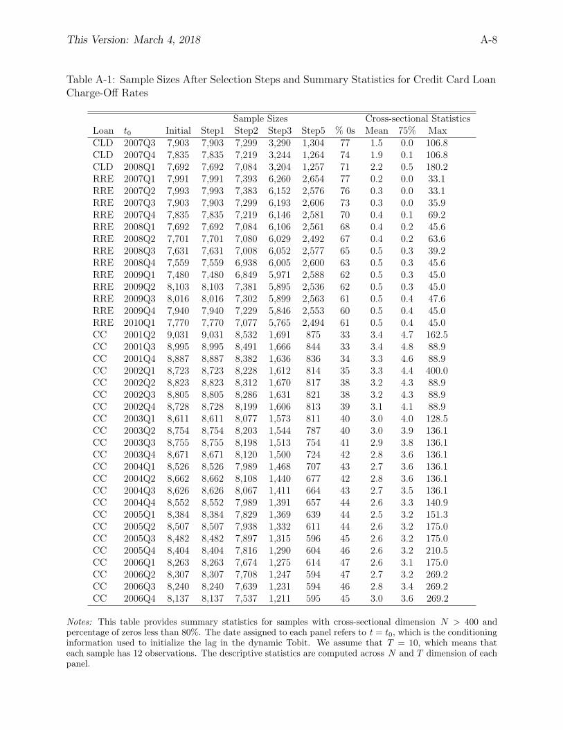
This Version: March 4, 2018 A-8
Table A-1: Sample Sizes After Selection Steps and Summary Statistics for Credit Card LoanCharge-Off Rates
Sample Sizes Cross-sectional StatisticsLoan t0 Initial Step1 Step2 Step3 Step5 % 0s Mean 75% MaxCLD 2007Q3 7,903 7,903 7,299 3,290 1,304 77 1.5 0.0 106.8CLD 2007Q4 7,835 7,835 7,219 3,244 1,264 74 1.9 0.1 106.8CLD 2008Q1 7,692 7,692 7,084 3,204 1,257 71 2.2 0.5 180.2RRE 2007Q1 7,991 7,991 7,393 6,260 2,654 77 0.2 0.0 33.1RRE 2007Q2 7,993 7,993 7,383 6,152 2,576 76 0.3 0.0 33.1RRE 2007Q3 7,903 7,903 7,299 6,193 2,606 73 0.3 0.0 35.9RRE 2007Q4 7,835 7,835 7,219 6,146 2,581 70 0.4 0.1 69.2RRE 2008Q1 7,692 7,692 7,084 6,106 2,561 68 0.4 0.2 45.6RRE 2008Q2 7,701 7,701 7,080 6,029 2,492 67 0.4 0.2 63.6RRE 2008Q3 7,631 7,631 7,008 6,052 2,577 65 0.5 0.3 39.2RRE 2008Q4 7,559 7,559 6,938 6,005 2,600 63 0.5 0.3 45.6RRE 2009Q1 7,480 7,480 6,849 5,971 2,588 62 0.5 0.3 45.0RRE 2009Q2 8,103 8,103 7,381 5,895 2,536 62 0.5 0.3 45.0RRE 2009Q3 8,016 8,016 7,302 5,899 2,563 61 0.5 0.4 47.6RRE 2009Q4 7,940 7,940 7,229 5,846 2,553 60 0.5 0.4 45.0RRE 2010Q1 7,770 7,770 7,077 5,765 2,494 61 0.5 0.4 45.0CC 2001Q2 9,031 9,031 8,532 1,691 875 33 3.4 4.7 162.5CC 2001Q3 8,995 8,995 8,491 1,666 844 33 3.4 4.8 88.9CC 2001Q4 8,887 8,887 8,382 1,636 836 34 3.3 4.6 88.9CC 2002Q1 8,723 8,723 8,228 1,612 814 35 3.3 4.4 400.0CC 2002Q2 8,823 8,823 8,312 1,670 817 38 3.2 4.3 88.9CC 2002Q3 8,805 8,805 8,286 1,631 821 38 3.2 4.3 88.9CC 2002Q4 8,728 8,728 8,199 1,606 813 39 3.1 4.1 88.9CC 2003Q1 8,611 8,611 8,077 1,573 811 40 3.0 4.0 128.5CC 2003Q2 8,754 8,754 8,203 1,544 787 40 3.0 3.9 136.1CC 2003Q3 8,755 8,755 8,198 1,513 754 41 2.9 3.8 136.1CC 2003Q4 8,671 8,671 8,120 1,500 724 42 2.8 3.6 136.1CC 2004Q1 8,526 8,526 7,989 1,468 707 43 2.7 3.6 136.1CC 2004Q2 8,662 8,662 8,108 1,440 677 42 2.8 3.6 136.1CC 2004Q3 8,626 8,626 8,067 1,411 664 43 2.7 3.5 136.1CC 2004Q4 8,552 8,552 7,989 1,391 657 44 2.6 3.3 140.9CC 2005Q1 8,384 8,384 7,829 1,369 639 44 2.5 3.2 151.3CC 2005Q2 8,507 8,507 7,938 1,332 611 44 2.6 3.2 175.0CC 2005Q3 8,482 8,482 7,897 1,315 596 45 2.6 3.2 175.0CC 2005Q4 8,404 8,404 7,816 1,290 604 46 2.6 3.2 210.5CC 2006Q1 8,263 8,263 7,674 1,275 614 47 2.6 3.1 175.0CC 2006Q2 8,307 8,307 7,708 1,247 594 47 2.7 3.2 269.2CC 2006Q3 8,240 8,240 7,639 1,231 594 46 2.8 3.4 269.2CC 2006Q4 8,137 8,137 7,537 1,211 595 45 3.0 3.6 269.2
Notes: This table provides summary statistics for samples with cross-sectional dimension N > 400 andpercentage of zeros less than 80%. The date assigned to each panel refers to t = t0, which is the conditioninginformation used to initialize the lag in the dynamic Tobit. We assume that T = 10, which means thateach sample has 12 observations. The descriptive statistics are computed across N and T dimension of eachpanel.

This Version: March 4, 2018 A-9
Table A-1: Sample Sizes After Selection Steps and Summary Statistics for Credit Card LoanCharge-Off Rates (cont.)
Sample Sizes Cross-sectional StatisticsLoan t0 Initial Step1 Step2 Step3 Step5 % 0s Mean 75% MaxCC 2007Q1 7,991 7,991 7,393 1,197 574 44 3.2 3.9 269.2CC 2007Q2 7,993 7,993 7,383 1,173 561 43 3.3 4.1 269.2CC 2007Q3 7,903 7,903 7,299 1,159 544 44 3.2 4.2 175.0CC 2007Q4 7,835 7,835 7,219 1,133 534 43 3.3 4.2 175.0CC 2008Q1 7,692 7,692 7,084 1,123 527 44 3.3 4.2 175.0CC 2008Q2 7,701 7,701 7,080 1,101 512 45 3.2 4.1 158.3CC 2008Q3 7,631 7,631 7,008 1,096 509 44 3.1 4.0 158.3CC 2008Q4 7,559 7,559 6,938 1,082 506 45 3.1 3.9 149.4CC 2009Q1 7,480 7,480 6,849 1,059 498 46 3.0 3.7 147.3CC 2009Q3 8,016 8,016 7,302 1,042 492 47 2.7 3.5 77.6CC 2009Q4 7,940 7,940 7,229 1,032 479 49 2.7 3.3 400.0CC 2010Q1 7,770 7,770 7,077 1,020 459 49 2.5 3.2 100.0CON 2009Q2 8,103 8,103 7,381 5,837 2,600 77 0.4 0.0 77.4CON 2009Q3 8,016 8,016 7,302 5,872 2,672 71 0.5 0.2 202.2CON 2009Q4 7,940 7,940 7,229 5,814 2,723 65 0.5 0.5 202.2CON 2010Q1 7,770 7,770 7,077 5,735 2,680 58 0.7 0.7 202.2
Notes: This table provides summary statistics for samples with cross-sectional dimension N > 400 andpercentage of zeros less than 80%. The date assigned to each panel refers to t = t0, which is the conditioninginformation used to initialize the lag in the dynamic Tobit. We assume that T = 10, which means thateach sample has 12 observations. The descriptive statistics are computed across N and T dimension of eachpanel.

This Version: March 4, 2018 A-10
C Additional Empirical Results
Figure A-1: Posterior Means of λi vs. σ2i
Normal π(λ), InvGam π(σ2) Flexible π(λ), π(σ2)
Notes: Credit card charge-off rates, heteroskedastic specification. The estimation sample for the dynamicTobit models ranges from 2001Q2 to 2003Q4 (T = 10).
Figure A-1 shoes that here is a cluster of banks for which λi is approximately 2.4 and
ln σ2i is approximately 1.5.

This Version: March 4, 2018 A-11
Figure A-2: Posterior Means of λi vs. σ2i
Normal π(λ), InvGam π(σ2) Flexible π(λ), π(σ2)
Notes: Credit card charge-off rates. The estimation sample for the dynamic Tobit models ranges from2001Q2 to 2003Q4 (T = 10).