formation evaluation of deep-water reservoirs in the 13a ... · in a water saturation model; an...
TRANSCRIPT

Formation Evaluation of Deep-water Reservoirs
in the 13A and 14A Sequences of the Central
Bredasdorp Basin, o�shore South Africa
by
Tarig M. Hamad Hussien
Thesis presented in partial ful�lment of the requirements for
the degree of Master of Science at the University of The
Western Cape
Department of Earth Sciences,
University of the Western Cape,
Bellville, South Africa.
Supervisor: Dr. Mimonitu Opuwari
November 2014

Abstract
Formation Evaluation of Deep-water Reservoirs in the 13A and
14A Sequences of the Central Bredasdorp Basin, o�shore South
Africa
T.M Hammad Hussien
Department of Earth Sciences,
University of the Western Cape,
Bellville, South Africa.
Thesis: MSc
November 2014
The goal of this study is to enhance the evaluation of subsurface reservoirs by improving
the prediction of petrophysical parameters through the integration of wireline logs and
core measurements. Formation evaluations of 13A and 14A sequences in the Bredasdorp
Basin, o�shore South Africa have been performed. Five wells in the central area of the
basin have been selected for this study.
Four di�erent lithofacies (A, B, C, D) were identi�ed, in the two cored wells, and used to
predict the lithofacies from wireline logs in uncored intervals and wells. A method based
on arti�cial neural network was used for this prediction. Facies A and B were recognized
as reservoir rocks and 13 reservoir zones were identi�ed and successfully evaluated in a
detailed petrophysical model.
The �nal shale volume was considered to be the minimum among �ve di�erent methods
applied in this study at any point along the well log. The porosity model was taken
from the density model. A value of 2.66 g/cm3 was obtained from core measurements as
the �eld average grain density, whereas the value of the �uid density of 0.79 g/cm3 was
obtained from core porosity and bulk density cross-plot.
i

ABSTRACT ii
In a water saturation model; an average water resistivity of 0.135 Ohm-m was estimated
from SP method. The calculated water saturation models were calibrated with core
measurements, and the Indonesia model best matched with the water saturation from
conventional core analysis.
Six hydraulic �ow units were recognized in the studied reservoirs, and were used for
permeability predictions. The permeability predicted from hydraulic �ow units were found
more reliable than the permeability calculated from porosity-permeability relationship.
The net pay was identi�ed for each reservoir by applying cut-o�s on permeability 0.1 mD,
porosity 7%, shale volume 0.35, and water saturation 0.60. The gross thickness of the
reservoirs ranges from 4.83m to 41.07m and net pay intervals from 1.21m to 29.59m.

Declaration
I declare that Formation Evaluation of Deep-Water Reservoirs in the 13A and 14A Se-
quences of the Central Bredasdorp Basin, o�shore South Africa is my own work, that
it has not been submitted before for any degree or examination in any other University,
and that all the sources I have used or quoted have been indicated and acknowledged by
means of complete references.
Tarig M. Hamad Hussien
November 2014
Signature ........................
iii

Acknowledgements
This work has reached its successful completion mainly because of the help of so many
people. I would like to express my sincere gratitude to my supervisor, Dr. Mimonito
Opuwari, for his guidance and assistance.
Special thanks to the Earth Science Department of University of the Western Cape, for
the use of their facilities to conduct my research.
To my parents for their understanding, and words of encouragement, during my research
which helped me focus my e�ort and bring it to conclusion.
My deepest appreciation to my dear wife Amany Kamblawe, who has always encouraged
me with love, patience, and understanding, I owe much of my success to her.
But above all, I would like to thank the Almighty Allah for everything that he has given
to me, for his blessings and guidance to �nish this work.
iv

Contents
Abstract i
Declaration iii
Acknowledgements iv
Contents v
List of Figures ix
List of Tables xii
1 Introduction 1
1.1 Preface . . . . . . . . . . . . . . . . . . . . . . . . . . . . . . . . . . . . . . 1
1.2 Aims of the study . . . . . . . . . . . . . . . . . . . . . . . . . . . . . . . . 2
1.3 Location of the study area . . . . . . . . . . . . . . . . . . . . . . . . . . . 2
1.4 Data set . . . . . . . . . . . . . . . . . . . . . . . . . . . . . . . . . . . . . 4
1.5 Thesis structure . . . . . . . . . . . . . . . . . . . . . . . . . . . . . . . . . 4
2 Geological Setting of the Bredasdorp Basin 5
2.1 The Structural Development of the Bredasdorp Basin . . . . . . . . . . . . 5
2.2 Stratigraphy and Sedimentology of the Bredasdorp Basin . . . . . . . . . . 8
2.2.1 Syn-rift Succession . . . . . . . . . . . . . . . . . . . . . . . . . . . 8
2.2.2 Drift Succession . . . . . . . . . . . . . . . . . . . . . . . . . . . . . 9
2.2.2.1 Transitional to early drift sequences . . . . . . . . . . . . 10
2.2.2.2 Late drift sequences . . . . . . . . . . . . . . . . . . . . . 10
3 Methodology and Materials 11
3.1 Methodology . . . . . . . . . . . . . . . . . . . . . . . . . . . . . . . . . . 11
3.2 Wireline Data . . . . . . . . . . . . . . . . . . . . . . . . . . . . . . . . . . 13
3.2.1 Depth shifting . . . . . . . . . . . . . . . . . . . . . . . . . . . . . . 13
3.2.2 Borehole Environmental Corrections . . . . . . . . . . . . . . . . . 14
v

CONTENTS vi
3.2.2.1 Gamma Ray (GR) . . . . . . . . . . . . . . . . . . . . . . 15
3.2.2.2 Neutron (NPHI) . . . . . . . . . . . . . . . . . . . . . . . 17
3.2.2.3 Density (RHOB) . . . . . . . . . . . . . . . . . . . . . . . 18
3.2.2.4 Deep Resistivity (LLD/ILD) . . . . . . . . . . . . . . . . . 19
3.2.3 Log Normalization . . . . . . . . . . . . . . . . . . . . . . . . . . . 19
3.2.4 Curve Splicing . . . . . . . . . . . . . . . . . . . . . . . . . . . . . . 20
3.3 Core Data . . . . . . . . . . . . . . . . . . . . . . . . . . . . . . . . . . . . 21
3.3.1 Well E-BB1 . . . . . . . . . . . . . . . . . . . . . . . . . . . . . . . 21
3.3.2 Well E-AO1 . . . . . . . . . . . . . . . . . . . . . . . . . . . . . . . 21
3.3.3 Conventional Core Analysis . . . . . . . . . . . . . . . . . . . . . . 21
3.4 Core-Log Depth Matching . . . . . . . . . . . . . . . . . . . . . . . . . . . 23
4 Facies, Sequence Boundaries and Reservoir Zones 24
4.1 Introduction . . . . . . . . . . . . . . . . . . . . . . . . . . . . . . . . . . . 24
4.2 Facies from Core . . . . . . . . . . . . . . . . . . . . . . . . . . . . . . . . 24
4.2.1 Massive sandstone (A) . . . . . . . . . . . . . . . . . . . . . . . . . 25
4.2.2 Shaly Sandstone (B) . . . . . . . . . . . . . . . . . . . . . . . . . . 25
4.2.3 Interbedded sandstone, siltstone and claystone (C) . . . . . . . . . 25
4.2.4 Massive Claystone (D) . . . . . . . . . . . . . . . . . . . . . . . . . 25
4.3 Facies from Wireline Logs . . . . . . . . . . . . . . . . . . . . . . . . . . . 27
4.3.1 Method of Facies Prediction . . . . . . . . . . . . . . . . . . . . . . 27
4.3.2 Results . . . . . . . . . . . . . . . . . . . . . . . . . . . . . . . . . . 28
4.4 Sequences Boundaries . . . . . . . . . . . . . . . . . . . . . . . . . . . . . . 32
4.5 Reservoir Zones Identi�cation . . . . . . . . . . . . . . . . . . . . . . . . . 34
4.5.1 E-AD1 Reservoir Zones . . . . . . . . . . . . . . . . . . . . . . . . . 34
4.5.2 E-AO1 Reservoir Zones . . . . . . . . . . . . . . . . . . . . . . . . . 36
4.5.3 E-AO2 Reservoir Zones . . . . . . . . . . . . . . . . . . . . . . . . . 38
4.5.4 E-BB1 Reservoir Zones . . . . . . . . . . . . . . . . . . . . . . . . . 39
4.5.5 E-BB2 Reservoir Zones . . . . . . . . . . . . . . . . . . . . . . . . . 39
5 Petrophysical Model 42
5.1 Volume of Shale Determinations . . . . . . . . . . . . . . . . . . . . . . . . 42
5.1.1 Resistivity Shale Volume . . . . . . . . . . . . . . . . . . . . . . . . 43
5.1.2 Gamma Ray Shale Volume . . . . . . . . . . . . . . . . . . . . . . . 43
5.1.3 Computed Gamma Ray Volume of Shale . . . . . . . . . . . . . . . 44
5.1.4 Correction of Shale Volume . . . . . . . . . . . . . . . . . . . . . . 45
5.1.5 Final Volume of Shale . . . . . . . . . . . . . . . . . . . . . . . . . 45
5.2 Porosity Determinations . . . . . . . . . . . . . . . . . . . . . . . . . . . . 47

CONTENTS vii
5.2.1 Core Porosity . . . . . . . . . . . . . . . . . . . . . . . . . . . . . . 47
5.2.2 Porosity from Density Log . . . . . . . . . . . . . . . . . . . . . . . 48
5.2.2.1 Matrix Density . . . . . . . . . . . . . . . . . . . . . . . . 48
5.2.2.2 Fluid Density . . . . . . . . . . . . . . . . . . . . . . . . . 49
5.2.3 Porosity from Sonic Log . . . . . . . . . . . . . . . . . . . . . . . . 50
5.2.4 Porosity from Density and Neutron Logs . . . . . . . . . . . . . . . 51
5.2.5 Core-Log Calibration . . . . . . . . . . . . . . . . . . . . . . . . . . 51
5.2.6 E�ective Porosity . . . . . . . . . . . . . . . . . . . . . . . . . . . 52
5.3 Saturation Determinations . . . . . . . . . . . . . . . . . . . . . . . . . . . 54
5.3.1 Water Saturation . . . . . . . . . . . . . . . . . . . . . . . . . . . . 54
5.3.1.1 Formation Temperature . . . . . . . . . . . . . . . . . . . 55
5.3.1.2 Formation Water Resistivity . . . . . . . . . . . . . . . . . 56
5.3.1.3 Pickett Plot . . . . . . . . . . . . . . . . . . . . . . . . . . 57
5.3.1.4 Core-log Calibration . . . . . . . . . . . . . . . . . . . . . 58
5.4 Permeability Determinations . . . . . . . . . . . . . . . . . . . . . . . . . . 60
5.4.1 Core Permeability . . . . . . . . . . . . . . . . . . . . . . . . . . . . 60
5.4.2 Core Permeability and Core Porosity Relationship . . . . . . . . . 61
5.4.3 Hydraulic Flow Units . . . . . . . . . . . . . . . . . . . . . . . . . . 62
5.4.3.1 Estimation of Hydraulic Flow Units Using Core Data . . . 62
5.4.3.2 Estimation of Flow Units in Uncored Intervals and Wells . 66
5.4.3.3 Permeability Prediction from Flow Units . . . . . . . . . . 68
6 Determination of Cut-O� and Net Pay 71
6.1 Cut-O� Determinations . . . . . . . . . . . . . . . . . . . . . . . . . . . . 71
6.1.0.4 Permeability Cut-O� . . . . . . . . . . . . . . . . . . . . . 72
6.1.0.5 Porosity Cut-O� . . . . . . . . . . . . . . . . . . . . . . . 72
6.1.0.6 Shale Volume Cut-O� . . . . . . . . . . . . . . . . . . . . 73
6.1.0.7 Water Saturation Cut-O� . . . . . . . . . . . . . . . . . . 74
6.2 Net Pay . . . . . . . . . . . . . . . . . . . . . . . . . . . . . . . . . . . . . 76
6.2.1 E-AD1 . . . . . . . . . . . . . . . . . . . . . . . . . . . . . . . . . . 76
6.2.2 E-AO1 . . . . . . . . . . . . . . . . . . . . . . . . . . . . . . . . . . 79
6.2.3 E-AO2 . . . . . . . . . . . . . . . . . . . . . . . . . . . . . . . . . . 80
6.2.4 E-BB1 . . . . . . . . . . . . . . . . . . . . . . . . . . . . . . . . . . 81
6.2.5 E-BB2 . . . . . . . . . . . . . . . . . . . . . . . . . . . . . . . . . . 81
7 Conclusions and recommendations 84
7.1 Conclusions . . . . . . . . . . . . . . . . . . . . . . . . . . . . . . . . . . . 84
7.2 Recommendations . . . . . . . . . . . . . . . . . . . . . . . . . . . . . . . . 85

CONTENTS viii
References 86
Appendices 91

List of Figures
1.1 Location map showing the Bredasdorp Basin, o�shore South Africa . . . . . . 3
1.2 Location map showing distribution of wells in this study across the centre of
the Bredasdorp Basin . . . . . . . . . . . . . . . . . . . . . . . . . . . . . . . 3
2.1 The Southern African o�shore basins . . . . . . . . . . . . . . . . . . . . . . . 6
2.2 Three schematic cross-sections across the Bredasdorp Basin . . . . . . . . . . 7
2.3 Stratigraphic chart of the Bredasdorp Basin. . . . . . . . . . . . . . . . . . . . 9
2.4 Rift faulting in the Bredasdorp Basin. . . . . . . . . . . . . . . . . . . . . . . 10
3.1 Research methodology �ow chart. . . . . . . . . . . . . . . . . . . . . . . . . . 12
3.2 Example of gamma ray log used as reference to check the depth shift in di�erent
datasets in E-AD1. . . . . . . . . . . . . . . . . . . . . . . . . . . . . . . . . . 14
3.3 Graphics of uncorrected and corrected gamma ray logs. . . . . . . . . . . . . . 16
3.4 Schlumberger gamma ray corrections chart . . . . . . . . . . . . . . . . . . . . 17
3.5 Graphics of uncorrected and corrected neutron logs. . . . . . . . . . . . . . . . 18
3.6 Graphics of uncorrected and corrected density logs. . . . . . . . . . . . . . . . 19
3.7 Graphics of uncorrected and corrected resistivity logs. . . . . . . . . . . . . . . 20
3.8 Uncorrected core porosity and corrected core porosity relationship for E-AO1. 22
3.9 Uncorrected core permeability and corrected core permeability relationship for
E-AO1. . . . . . . . . . . . . . . . . . . . . . . . . . . . . . . . . . . . . . . . 23
4.1 Core facies and gamma ray log in E-BB1 over a depth interval of about 2836m
to 2882m. . . . . . . . . . . . . . . . . . . . . . . . . . . . . . . . . . . . . . . 26
4.2 Core facies and gamma ray log in E-AO1 over a depth interval of about 2669m
to 2692m. . . . . . . . . . . . . . . . . . . . . . . . . . . . . . . . . . . . . . . 26
4.3 Input well logs GR, ILD, DT, NPHI, PEF, RHOB and core facies in E-AO1
over a depth interval of about 2662mto 2692m. . . . . . . . . . . . . . . . . . . 28
4.4 Input well logs GR, LLD, DT, NPHI, PEF, RHOB and core facies in E-BB1
over a depth interval of about 2843m to 2878m . . . . . . . . . . . . . . . . . 29
4.5 Correlation between core facies and wireline facies in E-AO1. . . . . . . . . . . 31
ix

LIST OF FIGURES x
4.6 Correlation between core facies and wireline facies in E-BB1. . . . . . . . . . . 31
4.7 The correlation between sequences boundaries of 13A and 14A units. . . . . . 33
4.8 Reservoir zone one in E-AD1. . . . . . . . . . . . . . . . . . . . . . . . . . . . 34
4.9 Reservoir zone two in E-AD1. . . . . . . . . . . . . . . . . . . . . . . . . . . . 35
4.10 Reservoir three one in E-AD1. . . . . . . . . . . . . . . . . . . . . . . . . . . . 35
4.11 Reservoir zone one in E-AO1. . . . . . . . . . . . . . . . . . . . . . . . . . . . 36
4.12 Reservoir zone two in E-AO1. . . . . . . . . . . . . . . . . . . . . . . . . . . . 36
4.13 Reservoir zone three in E-AO1. . . . . . . . . . . . . . . . . . . . . . . . . . . 37
4.14 Reservoir zone four in E-AO1. . . . . . . . . . . . . . . . . . . . . . . . . . . . 37
4.15 Reservoir zone one in E-AO2. . . . . . . . . . . . . . . . . . . . . . . . . . . . 38
4.16 Reservoir zone two in E-AO2. . . . . . . . . . . . . . . . . . . . . . . . . . . . 38
4.17 Reservoir zone one in E-BB1. . . . . . . . . . . . . . . . . . . . . . . . . . . . 39
4.18 Reservoir zone one in E-BB2. . . . . . . . . . . . . . . . . . . . . . . . . . . . 40
4.19 Reservoir zone two in E-BB2. . . . . . . . . . . . . . . . . . . . . . . . . . . . 40
4.20 Reservoir zone three in E-BB2. . . . . . . . . . . . . . . . . . . . . . . . . . . 41
5.1 (A) The GR logs of the four wells before normalization together with CGR
from E-AD1, (B) The same logs after normalization. . . . . . . . . . . . . . . 44
5.2 Shale volume calculation by using GR, GR Clavier et al, GR Steiber, CGR,
resistivity and �nal volume of shale in E-AO1 from depth 2555m to 2577m. . . 46
5.3 Shale volume calculation by using GR, GR Clavier et al, GR Steiber, CGR,
resistivity and �nal volume of shale in E-BB2 from depth 2535m to 2553m. . . 46
5.4 E-BB1 and E-AO1 core porosity (%) histogram. . . . . . . . . . . . . . . . . . 47
5.5 Core grain density histogram of wells E-AO1 and E-BB1. . . . . . . . . . . . . 49
5.6 Core porosity and density log cross-plot of E-AO1. . . . . . . . . . . . . . . . 50
5.7 Calculated porosities overlaying core porosity in E-BB1. . . . . . . . . . . . . 52
5.8 Calculated porosities overlaying core porosity in E-AO1. . . . . . . . . . . . . 53
5.9 Pickett Plot for determination of exponent (n) and cementation exponent (m)
for well E-AD1. . . . . . . . . . . . . . . . . . . . . . . . . . . . . . . . . . . . 58
5.10 Comparison of core and log water saturation models for Well E-BB1. . . . . . 59
5.11 Comparison of core and log water saturation models for Well E-AO1. . . . . . 59
5.12 E-BB1 and E-AO1 core permeability (mD) histogram. . . . . . . . . . . . . . 60
5.13 The correlation between core porosity and core permeability of E-BB1 and
E-AO1. . . . . . . . . . . . . . . . . . . . . . . . . . . . . . . . . . . . . . . . 61
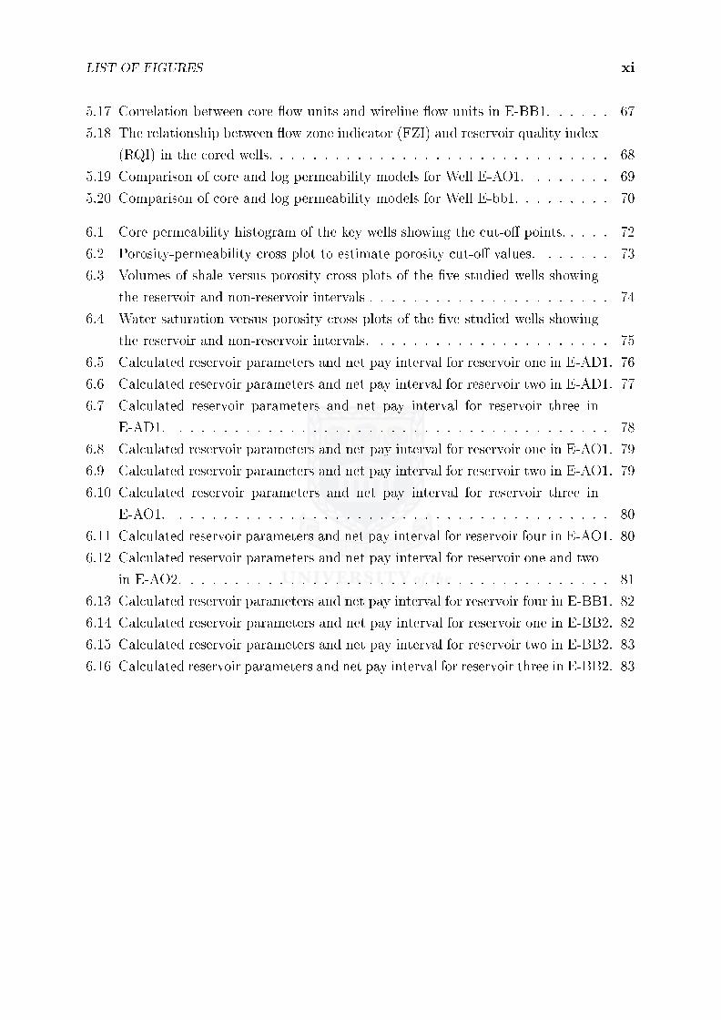
5.14 Plot of RQI versus NPI for the cored interval of E-AO1 and E-BB2 resulting
in six di�erent �ow units. . . . . . . . . . . . . . . . . . . . . . . . . . . . . . 65
5.15 A histogram of FZI and calculated �ow units. . . . . . . . . . . . . . . . . . . 65
5.16 Correlation between core �ow units and wireline �ow units in E-AO1. . . . . . 67
LIST OF FIGURES xi
5.17 Correlation between core �ow units and wireline �ow units in E-BB1. . . . . . 67
5.18 The relationship between �ow zone indicator (FZI) and reservoir quality index
(RQI) in the cored wells. . . . . . . . . . . . . . . . . . . . . . . . . . . . . . . 68
5.19 Comparison of core and log permeability models for Well E-AO1. . . . . . . . 69
5.20 Comparison of core and log permeability models for Well E-bb1. . . . . . . . . 70
6.1 Core permeability histogram of the key wells showing the cut-o� points. . . . . 72
6.2 Porosity-permeability cross plot to estimate porosity cut-o� values. . . . . . . 73
6.3 Volumes of shale versus porosity cross plots of the �ve studied wells showing
the reservoir and non-reservoir intervals . . . . . . . . . . . . . . . . . . . . . . 74
6.4 Water saturation versus porosity cross plots of the �ve studied wells showing
the reservoir and non-reservoir intervals. . . . . . . . . . . . . . . . . . . . . . 75
6.5 Calculated reservoir parameters and net pay interval for reservoir one in E-AD1. 76
6.6 Calculated reservoir parameters and net pay interval for reservoir two in E-AD1. 77
6.7 Calculated reservoir parameters and net pay interval for reservoir three in
E-AD1. . . . . . . . . . . . . . . . . . . . . . . . . . . . . . . . . . . . . . . . 78
6.8 Calculated reservoir parameters and net pay interval for reservoir one in E-AO1. 79
6.9 Calculated reservoir parameters and net pay interval for reservoir two in E-AO1. 79
6.10 Calculated reservoir parameters and net pay interval for reservoir three in
E-AO1. . . . . . . . . . . . . . . . . . . . . . . . . . . . . . . . . . . . . . . . 80
6.11 Calculated reservoir parameters and net pay interval for reservoir four in E-AO1. 80
6.12 Calculated reservoir parameters and net pay interval for reservoir one and two
in E-AO2. . . . . . . . . . . . . . . . . . . . . . . . . . . . . . . . . . . . . . . 81
6.13 Calculated reservoir parameters and net pay interval for reservoir four in E-BB1. 82
6.14 Calculated reservoir parameters and net pay interval for reservoir one in E-BB2. 82
6.15 Calculated reservoir parameters and net pay interval for reservoir two in E-BB2. 83
6.16 Calculated reservoir parameters and net pay interval for reservoir three in E-BB2. 83

List of Tables
3.1 E-BB1 Cored Intervals within 13A and 14A sequences. . . . . . . . . . . . . . 21
3.2 E-AO1 Cored Intervals within 13A and 14A sequences. . . . . . . . . . . . . . 21
3.3 Core-log depth shift for E-BB1 and E-AO1 wells. . . . . . . . . . . . . . . . . 23
4.1 Normalized minimum and maximum values for input logs of the studied wells. 29
4.2 The statistic of predicted facies . . . . . . . . . . . . . . . . . . . . . . . . . . 30
4.3 The correlation factor and the contribution of each input log. . . . . . . . . . 30
4.4 Sequences boundaries in the investigated wells. . . . . . . . . . . . . . . . . . 32
5.1 The minimum and maximum values of gamma ray logs (GR), computed gamma
ray logs (CGR) and resistivity logs (ILD/LLD) used in shale volume calculations. 45
5.2 Water saturation equations used in the study. . . . . . . . . . . . . . . . . . . 55
5.3 Water saturation equations used in the study. . . . . . . . . . . . . . . . . . . 57
5.4 E-BB1 Calculated values for RQI, NPI and FZI. . . . . . . . . . . . . . . . . . 63
5.5 E-AO1 Calculated values for RQI, NPI and FZI . . . . . . . . . . . . . . . . . 64
5.6 The range and the mean of FZI within the calculated �ow units. . . . . . . . . 66
6.1 Summary of calculated reservoir pay parameters for E-AD1 . . . . . . . . . . . 77
6.2 Summary of calculated reservoir pay parameters for E-AO1 . . . . . . . . . . . 79
6.3 Summary of calculated reservoir pay parameters for E-AO2 . . . . . . . . . . . 80
6.4 Summary of calculated reservoir pay parameters for E-BB1 . . . . . . . . . . . 81
6.5 Summary of calculated reservoir pay parameters for E-BB2 . . . . . . . . . . . 81
xii

Chapter 1
Introduction
1.1 Preface
Formation evaluation is the process of interpreting a combination of measurements taken
inside a porehole to detect and quantify hydrocarbon reserves in the strata adjacent to
the porehole. It also involves determining of both, physical and chemical properties of
rocks and the �uids they contain. This evaluation mainly depends on wireline logs which
measure these various physical and chemical properties of the formations (Alger, 1980).
These logs are commonly used for the determination of certain petrophysical properties
of rocks such as porosity, permeability, water saturation and possibly pore geometry.
The petrophysical evaluation of subsurface strata also involves integration of di�erent
datasets from multiple disciplines for better reservoir description (Gunter et al., 1997).
Normally, geologists use core measurements, seismic and well testing to improve the wire-
line petrophysical model. Core data presents an important means to calibrate a petro-
physical model as it provides vital information unavailable from either wireline logs or
productivity tests (Al-Saddique et al., 2000).
The Bredasdorp Basin is located o� the south coast of South Africa. Five wells in the
central area of the basin have been chosen for this study. The purpose of this study is to
describe, characterize and quantify the reservoir properties of the basin by integrating the
sedimentary facies characteristics and petrophysical properties. The study investigates the
relationships between primary depositional facies and petrophysical properties; porosity,
permeability and saturation.
1

1.2. Aims of the study 2
1.2 Aims of the study
The main aim of any reservoir characterization is to quantify and describe the spatial
distribution of petrophysical parameters, such as shale volume, porosity, permeability,
and saturations for the purpose of de�ning �ow units within it. Accurate knowledge
of these parameters for any hydrocarbon reservoir is required for e�cient development,
management, and prediction of future performance of the oil �eld. Wireline logs o�er the
opportunity for determining the petrophysical parameters, while core data presents an
important means to calibrate the petrophysical model.
The main goal of this research is to perform a complete characterization of the central
Bredasdorp Basin through the integration and comparison of results from core analysis
and petrophysical studies. The sand zones in the Bredasdorp Basin are considered as
low permeability reservoirs. Reservoir characterization is the key for understanding the
primary depositional facies which may control this low permeability. Another challenge
is predicting of facies from wireline log using neural networks.
The process for achieving a complete characterization requires the following:
- Perform data quality control through the environmental corrections for wireline logs and
overburden corrections for core data.
- To investigate the reservoir sedimentological characteristics of the basin strata and
predict the lithofacies.
- Estimate petrophysical properties from the wire line logs data.
- To calculate the net pay of the studied reservoirs.
1.3 Location of the study area
The Bredasdorp Basin is located o� the south coast of South Africa. The basin is the
most south-westerly of the Southern African o�shore basins as presented in �gure 1.1
below. The study area of this project is situated in the central part of the basin. Five
wells were selected for this research: E-AD1, E-AO1, E-AO2, E-BB1 and E-BB2. Figure
1.2 shows the distribution of the studied wells across the centre of the Bredasdorp Basin.

1.3. Location of the study area 3
Figure 1.1: Location map showing the Bredasdorp Basin, o�shore South Africa (modi�edfrom (McLachlan and McMillan, 1976).
Figure 1.2: Location map showing distribution of wells in this study across the centre ofthe Bredasdorp Basin (modi�ed from (Burden and Davies, 1997)).

1.4. Data set 4
1.4 Data set
The collected data for this study was classi�ed into two main groups:
1. Wireline logs of the �ve studied wells.
2. Core analysis data from two wells E-AO1 and E-BB1.
All data has been provided by the Petroleum Agency of South Africa (PASA). The details
of the data is given in chapter three.
1.5 Thesis structure
This thesis represents the written report of the research carried out to evaluate the hy-
drocarbon potential of 13A and 14A sequences in the central part of the Bredasdorp
Basin.
In chapter one a general introduction to the study is given. The structure and sequences
stratigraphy of the Bredasdorp Basin are brie�y reviewed in the second chapter. The
third presents the methodology of the study, with the corrections applied to the core
and wireline data. Facies predictions from both core data and wireline logs are discussed
in chapter four. Chapter four also includes determinations of the sequence boundaries
of the studied interval and determinations of reservoirs zones within the interval. The
petrophysical model is presented in detail in chapter �ve. Chapter six presents the deter-
minations of the cut-o� values and net pay of the studied reservoirs. With chapter seven
covering remarks and conclusions drawn from the study.

Chapter 2
Geological Setting of the Bredasdorp
Basin
In this chapter, a description of the Bredasdorp Basin is presented. This description
introduces the structural development in favour of a detailed study of the stratigraphy,
from which the sedimentation history might be determined. The Bredasdorp Basin is
located o� the south coast of South Africa, beneath the Indian Ocean. It covers about
18, 000km2 (200km long and 80km wide) (McMillan et al., 1997).
2.1 The Structural Development of the Bredasdorp
Basin
The South African coastline has a total length of about 3000 km. The west coast from the
Orange River to Cape Point is almost 900 km long and the remainder, from Cape Point
to the Mozambique border, is more than 2000 km long (PASA, 2008). The continental
margin, along this coastline, formed as a result of the separation of South America,
Africa and the Falkland Plateau (McMillan et al., 1997; Liro and Dawson, 2000). Three
major o�shore basins developed in western, southern and eastern South Africa, these are
respectively the: Orange, Outeniqua and Durban basins (PASA, 2005).
The Outeniqua Basin in particular, developed as a result of the right-lateral shear move-
ment along the Falkland-Agulhas Fracture Zone, which resulted in the separation of the
Falkland Plateau from the Mozambique Ridge, and the break-up of west Gondwana (South
America and Africa) during the Jurassic period (Tinker et al., 2008). During this time
the normal faulting resulted in the graben and half-graben basins (Brown et al., 1995).
5

2.1. The Structural Development of the Bredasdorp Basin 6
The Outeniqua Basin is bounded to the west by the Columbine-Agulhas Arch, to the east
by the Port Alfred Arch, and to the south by the Diaz Marginal Ridge. It comprises of
a series of rift sub-basins which are separated by fault-bounded Basement arches. These
are, from east to west; Algoa, Gamtoos, Pletmos, and the Bredasdorp basins. Figure 2.1
shows the Southern African coastline, and the o�shore basins and sub-basins.
Figure 2.1: (The Southern African o�shore basins (modi�ed from (PASA, 2003))
The Bredasdorp Basin can be described as a wide depression basement. The major
structural features of the Bredasdorp Basin are the normal faults. These faults present
a WNW-ESE trend, and bound half-grabens and structural highs throughout the basin
(�gure 2.2) (De Wit and Ransome, 1992). In general, the half-graben feature is developed
when normal faults are dipping in the same direction making adjacent fault blocks to slip
down and tilt relative to the fault next to it (Schalkwyk, 2005).
The break-up of Gondwana produced extensional stress, which led to the formation of the
pull-apart basin represented in the Outeniqua Basin. This followed by the right-lateral
movement along the Agulhas-Falkland Fracture Zone led to the creation of the half-graben
sub-basins including the Bredasdorp Basin.

2.1. The Structural Development of the Bredasdorp Basin 7
Figure 2.2: Three schematic cross-sections across the Bredasdorp Basin (from (Thomson,1998)).

2.2. Stratigraphy and Sedimentology of the Bredasdorp Basin 8
2.2 Stratigraphy and Sedimentology of the
Bredasdorp Basin
The deposition in the Bredasdorp Basin is mainly controlled by the initial continental
rifting and tectonic development. According to (McMillan et al., 1997) this rifting phase
was followed by a transitional episode and then a drifting episode. A regionally correlat-
able unconformity 1At1 terminated the active rift tectonics and separates the syn-rift and
post-rift sequences. The deposition of sediments in theses successions has been mainly
controlled by global sea level change. The description of these successions is discussed in
further detail further in this chapter. The stratigraphic chart of the Bredasdorp Basin is
presented in �gure 2.3.
2.2.1 Syn-rift Succession
The sedimentation rate of this sequence, which is bounded by horizon D and 1At1, was
strongly in�uenced by the di�erential subsidence of the basement �oor. All lithogenetic
units, which consist of Late Jurassic to Early Cretaceous-aged sediments, rest uncon-
formably on faulted basement within graben and condense over horsts (Figure 2.4).
The sediments within this interval consist of alluvial and channel �uvial deposits that
accumulated with faulting (Burden, 1992). (McMillan et al., 1997) identi�ed four litho-
genetic units in the rift sediments in the Bredasdorp Basin, these are:
1. The lower �uvial unit. This unit consists of red and minor green argillite with subor-
dinate reddish sandstones and rare conglomerates.
2. The lower shallow marine unit. This unit is considered to be the �rst marine deposit
in the basin. It occurred at an erosional regional unconformity marked by the appearance
of glauconitic, clean, �ne grained sandstones.
3. The upper �uvial unit. This unit overlying the shallow marine sediments, it consists
of interbedded non-glauconitic sandstones, red and green claystones, and siltstones.
4. The upper shallow marine unit. This unit was deposited in the second marine trans-
gression, and it is characterized by the second occurrence of the glauconitic sandstones.
The deposition of syn-rift sediments was followed by a tectonically controlled break in
sedimentation. The erosion of rift sediments during this period resulted in the formation
of 1At1 unconformity.

2.2. Stratigraphy and Sedimentology of the Bredasdorp Basin 9
Figure 2.3: Stratigraphic chart of the Bredasdorp Basin (from Burden, 1992).
2.2.2 Drift Succession
The sea level rise after the rifting phase established an open marine environment in the
Bredasdorp Basin during Mid-Cretaceous. These conditions allowed for deposits of shelf

2.2. Stratigraphy and Sedimentology of the Bredasdorp Basin 10
Figure 2.4: Rift faulting in the Bredasdorp Basin ((PASA, 2003)).
and slope shales, and channelised sandstone.
According to (McMillan et al., 1997), this sequence, from 1At1 to present, is divided into
two intervals:
1. Transitional to early drift sequences.
2. Late drift sequence.
2.2.2.1 Transitional to early drift sequences
These sequences bounded on the bottom and top by 1At1 and 13At1 unconformities
respectively. It considered as the �rst deep water deposits in the Bredasdorp Basin,
deposits as result of major subsidence of the basin, and the increase of water depth.
Deep-water environment sedimentation took place with low oxygen levels due to poor
circulation in the overlying water column (McMillan et al., 1997).
2.2.2.2 Late drift sequences
These sequences followed a major marine regression in the Bredasdorp Basin during early
Aptian. This regression caused signi�cant erosion marked by the regional 13At1 uncon-
formity. The marine transgression following this erosion carried organic rich claystone
deposited under low oxygen conditions (McMillan et al., 1997).

Chapter 3
Methodology and Materials
This chapter describes the methodology and materials used to conduct the research
project. The data available for the study is listed, with an outline of the various methods
used to correct the data. The collected data is classi�ed into two main groups: wireline
logs of the �ve studied wells, and core analysis data from two wells. All the data has been
provided by the Petroleum Agency of South Africa (PASA).
3.1 Methodology
Figure 3.1 presents the �ow chart of the various methods used in this study. The process
followed the following sequence:
1. Review the previous studies on the Bredasdorp Basin to become familiar with the basin
tectonic history and structural features. The review also includes sequence stratigraphy
studies of the basin, to understand the evolution of the sedimentary environment.
2. Develop a geological model based on the core data and wireline logs. The core data is
used to identify the lithofacies; then the integration between core and wireline logs is used
to calculate the electrofacies for all studied wells. The wireline logs and the calculated
electrofacies are used to infer sequences boundaries.
3. Develop a petrophysical model dependent on wireline logs and core data to determine
shale volume porosity, permeability and water saturation.
4. The petrophysical model is then used for determinations of cut-o�s and net pay within
the studied reservoirs to identify the hydrocarbons intervals.
5. Develop written report.
11

3.1. Methodology 12
Figure 3.1: Research methodology �ow chart.
The available data was carefully arranged and imported into Techlog software and the
required corrections were done when necessary. The details of each data set, and the
applied corrections are described and discussed further in this chapter.

3.2. Wireline Data 13
3.2 Wireline Data
Wireline logs were collected from the �ve studied wells penetrating the central Bredasdorp
Basin sandstones; the logging was carried out by Schlumberger Company in all the wells.
The logs were provided in LAS �le format, and only twelve of the many possible logs were
used as primary logs in this study. The logs used were:
� The Caliper (CL)
� Gamma Ray (GR)
� Spontaneous Potential (SP)
� Microspherically Focussed (MSFL)
� Deep Laterolog (LLD)
� Shallow Laterolog (LLS)
� Medium Laterolog (LLM)
� Deep Induction (ILD)
� Shallow Induction (ILS)
� Density (RHOB)
� Neutron (NPHI)
� Sonic logs (DT)
The digital suites of the logs were imported into the Techlog software workstation. Before
processing interpretation, the quality of the logs were checked, and editing performed
where required. The editing included for following: depth shifting, environmental correc-
tions, normalization, and curve splicing.
3.2.1 Depth shifting
Reservoir characterization involves the integration of wireline data from di�erent tools
runs. Consequently, measurements of formation properties from di�erent tools runs must
be depth shifted so that a log plot of formation properties versus depth puts all the
properties at the correct location (Moake, 2008). The di�erence between logs recorded in
the same borehole may exist due to borehole irregularities and tool type (Bassiouni, 1994).

3.2. Wireline Data 14
Normally the logs which have been logged during the same logging run are considered to
be in depth, and no depth shifting is required for them.
For this study, all logging runs were depth checked, the gamma ray logs were assumed
to be the reference depth and two shale zones were used as correlation markers. When
a gamma ray log is run on more than one tools run the reference gamma ray is chosen
based on cable tension and cable speed. A single log has been chosen from each logging
run to depth match against the depth reference log. Both logs were displayed side by side
to allow visual correlation and de�ne appropriate shift. In �gure 3.2 , seven di�erent logs
from di�erent data sets in E-AD1 are plotted together. All the logs are in depth except
RHOB in track 7, which is 3.32 m shallower.
Figure 3.2: Example of gamma ray log used as reference to check the depth shift in di�erentdatasets in E-AD1.
3.2.2 Borehole Environmental Corrections
The objective of logging is to obtain undisturbed values for the formation properties.
This is hardly accomplished because the drilling processes disturb the formation near the
borehole. Borehole e�ects on wireline logs can be divided into those produced by borehole

3.2. Wireline Data 15
geometry, drilling �uids conditions and mud cake. These parameters must be controlled
to improve the quality of wireline logs data.
Rough or rugose borehole walls have the largest in�uences in the logs responds, the e�ect
of enlarged borehole size on logs can be signi�cant and it a�ects most logs to greater
or lesser extent. Borehole enlargement beyond the bit size in�uences the reading of
centralized tools, while rugose borehole in�uences pad type tools. Therefore, the borehole
diameter is the mandatory input in any environmental correction procedure.
In this project environmental corrections were performed to compensate for most of the
unwanted borehole e�ects.
3.2.2.1 Gamma Ray (GR)
Any material with non-zero density in the annular space between the walls of the borehole
and the gamma ray detectors represents a disruptive environment to the measurement
process. This medium will a�ect the tool readings by certain degrees of ray scattering
and absorption, and thus decrease the �nal count rate (Lehmann, 2010).
Gamma ray environmental corrections have been historically presented in di�erent forms
using di�erent assumptions. Open hole conditions have been applied to the studied wells
measurements to compensate for hole size, mud weight and tool position. The corrections
corrections in this study have been performed using both the Techlog software environmen-
tal corrections module and Schlumberger log interpretation charts book for comparisons.
The essential input parameters were raw gamma ray logs, borehole diameter and �uid
density.
Figure 3.3 presents an example of an uncorrected gamma ray log and environmentally
corrected log for E-OA1 borehole. The green curve is the uncorrected gamma ray log,
while the blue curve is the corrected one. In track one; caliper and bit size are plotted to
show the e�ect of the borehole enlargement.

3.2. Wireline Data 16
Figure 3.3: Graphics of uncorrected and corrected gamma ray logs.
Figure 3.4 below represents Schlumberger gamma ray corrections chart for hole size and
mud weight (Schlumberger, 1989). The input parameter (t) in g/cm2, is calculated as
follows:
t =mudw
8.345
(2.54(holed)
2− 2.54(toold)
2
)(3.1)
where:
t: The input parameter (g/cm2)
mudw : Mud weight (lb/gal)
holed: Hole diameter (in)
toold : Tool diameter (in)
For comparison with Figure 3.3 in depth 1424.40m gamma ray reads 67.63 API units.
The input parameter (t) is 16.3 g/cm2 ( mud weight 1.1 Gram per Cubic Centimetre

3.2. Wireline Data 17
(g/cm3) equal to 9.18 pounds per gallon (lb/gal) resulting in a correction factor of 1.60.
Therefore the corrected gamma ray is 108.20 API units, which is equal to the calculated
value (107.25 API).
Figure 3.4: Schlumberger gamma ray corrections chart (modi�ed from (Schlumberger,1989)).
3.2.2.2 Neutron (NPHI)
The dual-detector, neutron porosity tools with ratio method used on the studied wells
logging were �rst produced to reduce environmental e�ects on the measurement, but it is
still necessary to apply corrections for certain borehole conditions (Galford et al., 1988).
The logs need corrections for formation temperature, formation pressure, borehole salinity
and mud weight.
For the studied wells, the raw near and far neutron count rate curves were used for
corrections. The input parameters also include mud temperature curve, borehole salinity
and borehole pressure.
The borehole pressure was calculated using mud weight and measured depth as replace-
ment of the true vertical depth (TVD), and the borehole size was corrected by the service
company during the logging.
Figure 3.5 shows an example of an uncorrected neutron log (red) and environmentally
corrected log (blue) for E-OA1 borehole.

3.2. Wireline Data 18
Figure 3.5: Graphics of uncorrected and corrected neutron logs.
3.2.2.3 Density (RHOB)
The density log is run eccentered with a pad bushing against the borehole wall. It is
therefore a�ected by the rough borehole wall. Generally, the environmental e�ects that
can in�uence the density tools are few in number, and the corrections are of very small
magnitude (Ellis and Singer, 2008).
In the current study, the density logs have been corrected to the hole size and mud weight,
Figure 3.6 is an example of an uncorrected density log (red) and environmentally corrected
log (blue) for E-BB1 borehole.

3.2. Wireline Data 19
Figure 3.6: Graphics of uncorrected and corrected density logs.
3.2.2.4 Deep Resistivity (LLD/ILD)
To achieve accurate saturation results several environmental corrections must be done to
resistivity tools. The tools measurements are sensitive to the borehole, and the applied
corrections include hole size and mud resistivity. Mud resistivity at any point along the
borehole is calculated using the mud sample resistivity and temperature from the LAS
�les header and the temperature logs.
Figure 3.7 shows an example of an uncorrected resistivity log (red) and environmentally
corrected log (blue) for E-BB1 borehole.
3.2.3 Log Normalization
Normalization is statistical analysis aim to minimize the di�erences in log measurements
caused by logging errors. Di�erences in log responses to identical formation conditions
may be caused by numbers of factors including; inaccurate tool calibration, di�erences in
tool types and when environmental corrections did not exactly match the actual logging
conditions (Clu� and Clu�, 2004). The normalization procedure to compensate all logs
of a particular type for these conditions involves using representative lithological zones in
each well so that they have similar characteristics over the selected intervals.
The selection of such lithological zones to use as reference for normalization is crucial; it
is di�cult to �nd zones that have similar rock properties throughout an area or �eld. In

3.2. Wireline Data 20
Figure 3.7: Graphics of uncorrected and corrected resistivity logs.
this project, since the studied wells have logged with the same service company and same
tools, and since the environmental corrections have been done carefully; no normalization
procedure was done. However, to identify facies from well logs which for qualitative
analysis, normalization has been performed to the logs involved in the procedure.
3.2.4 Curve Splicing
After performing the corrections, for any particular log type, the di�erent runs logged in
the same borehole were spliced together into a continuous log.

3.3. Core Data 21
3.3 Core Data
The core data consists of conventional core analysis and lithological description reports.
Only two of the �ve studied wells had core data available for this study, E-BB1 and E-
AO1. The total thickness of the sedimentary sections recovered from wells E-BB1 and
E-AO1 were 15.1m and 8.9 m respectively.
3.3.1 Well E-BB1
Eight cores were cut in this borehole two, within the interval of interest (sequences 13A
and 14A), were available for this study. Table 3.1 indicates the cored intervals of well
E-BB1.
Table 3.1: E-BB1 Cored Intervals within 13A and 14A sequences.
core Cored Interval (m) Cut (m) Recovery Recovered SequenceTop Bottom (%) (m)
5 2846.0 2864.0 18 58 10.44 13A6 2872.0 2877.0 5 92.6 4.63 13A
3.3.2 Well E-AO1
Six cores were cut in this borehole, one of them within the interval of interest (sequences
13A and 14A). The table below shows the cored intervals of well E-AO1.
Table 3.2: E-AO1 Cored Intervals within 13A and 14A sequences.
core Cored Interval (m) Cut (m) Recovery Recovered SequenceTop Bottom (%) (m)
1 2674 2683.25 9.25 96.75 8.9 13A
3.3.3 Conventional Core Analysis
The available conventional core analysis measurements include: porosity (%), liquid and
air permeabilities (mD), �uid saturations (%) and grain density (g/cc). For E-AO1 the
core data also included the overburden measurements of porosity and permeability. The
provided core measurements were digitalized and entered into a spreadsheet database for
processing. The raw conventional core analysis measurements for E-BB1 and E-AO1 is
given in Appendix A and B.

3.3. Core Data 22
Overburden corrections were applied to E-BB1 core data to simulate in situ reservoir
conditions by making use of the provided E-AO1 overburden porosities and permeabilities.
Figure 3.8 presents the relationship between the uncorrected and corrected porosities for
E-AO1. The empirical linear relationship is given by the regression equation:
Φcorrected = 0.9905385 ∗ Φuncorrected − 0.5127908 (3.2)
where:
Φcorrected is the core porosity at overburden pressure.
Φuncorrected is the core porosity at room condition.
Figure 3.8: Uncorrected core porosity and corrected core porosity relationship for E-AO1.
The same procedure has been done for permeability corrections (Figure 3.9). The regres-
sion equation is:
log10(Kcorrected) = 1.098863 ∗ log10(Kuncorrected) − 0.1403815 (3.3)
where:
Kcorrected is the core permeability at room condition.
Kuncorrected is the core permeability at overburden pressure.
These two equations have been used to correct the porosity and permeability values for
the other cored well E-BB1, the corrected values are given in Appendix C.

3.4. Core-Log Depth Matching 23
Figure 3.9: Uncorrected core permeability and corrected core permeability relationship forE-AO1.
3.4 Core-Log Depth Matching
Wireline logging and coring are two di�erent processes. Logs are identi�ed by Wireline
depths; core by driller depths and the measurements are carried out by di�erent service
provider at di�erent times. This implies di�erences between the two measured depths.
Therefore, the core depth should be depth matched to the wireline depth (Worthington,
1991).
In this study, a correction based on correlation between gamma ray log and a reference
shale point has been done. The conventional core analysis results have been compared to
the log data by overlaying core measured data and wireline logs data, core depths have
been shifted to match the wireline depths
The table below shows the required shift in each cored interval to match the log data.
Table 3.3: Core-log depth shift for E-BB1 and E-AO1 wells.
Well Core Cored Interval (m) Corrected Interval (m) ShiftTop Bottom Top Bottom
E-BB1 5 2846 2864 2848 2866 2E-BB1 6 2872 2877 2874.5 2879.5 2.5E-AO1 1 2674 2683.25 2674.3 2683.55 0.3

Chapter 4
Facies, Sequence Boundaries and
Reservoir Zones
4.1 Introduction
In exploration and production of hydrocarbon from sedimentary basins the full under-
standing of the properties of subsurface strata is essential. For better evaluation of hy-
drocarbon reservoirs, facies are of great importance. This importance rests upon their
control of the variation of petrophysical properties and subsurface �uid �ow (Yumei,
2006).
Facie refers to a body of rocks with unique lithological, physical, and biological attributes
relative to all adjacent deposits (Octavian, 2006) . It re�ects the physical, chemical and
biological conditions and processes of the depositional environment.
The core data provided the basis on which sedimentologic observation and interpretation
are established because reservoir properties are directly measured on core samples. It is
normally the most reliable petrophysical data.
4.2 Facies from Core
Within the studied wells, the central Bredasdorp Basin has only three cores through the
interval stratigraphy of 13A and 14A sequences available for this study. The sedimento-
logical descriptions which were carried out by SOEKOR were used to determine facies
distribution based on nearly 24m of the available cores. The facies have been classi�ed
based on grain size, textures, primary and secondary sedimentary structures.
24

4.2. Facies from Core 25
Four distinct facies types have been distinguished in the studied wells. These facies were
alphabetically designated, A through D, and are discussed further in this chapter.
4.2.1 Massive sandstone (A)
Clean massive sandstone characterised by very �ne to medium grained, well sorted sands.
No grading of the grain size can be detected. The sandstones are generally massive with
rare sedimentary structure such as ripple strati�cation. This facies occurs in core 5 in
E-BB1 from depth 2847.2m to 2857.5m (logger depth) and from 2872.2m to 2872.6m
as presented in �gure 4.1. This facies is interpreted to be the basal part of channel-�ll
sandstone deposited on a submarine fan in an inner fan to middle fan setting.
4.2.2 Shaly Sandstone (B)
This facies is also massive sandstone, but it is characterised by occasionally thin claystone
interbeds. These claystones do not exceed 5cm and have sharp tops. The sandstone is
very argillaceous, light to dark grey, �ne to very �ne grained with abundant claystone
clasts. The sandstone individual beds vary in thickness from 0.2m to 1.3m or even more.
This facies occurs in core 1 in E-AO1 from depth 2674.3m to 2681.3m as shown in �gure
4.2.
4.2.3 Interbedded sandstone, siltstone and claystone (C)
The claystone in this facies is massive, dark grey to black and interbedded in millimetre
to centimetre scale with argillaceous sandstone and siltstone. Carbonaceous materials are
present in minor amounts. The interbedded sandstones are generally massive with sharp
upper contacts. This facies occurs in core 1 in E-AO1 from depth 2681.4m to 2683.5m and
in core 6 in E-BB1 from 2872.7m to 2874m as presented in �gures 4.1 and 4.2 respectively.
4.2.4 Massive Claystone (D)
This facies is characterised by greyish black to dark grey claystone. The claystone is
generally homogenous with occasionally very thin siltstone laminae of millimetre scale.
This facies occurs in core 6 in E-BB1 from depth 2874.3m to 2976.9m as shown in �gure
4.1.

4.2. Facies from Core 26
Figure 4.1: Core facies and gamma ray log in E-BB1 over a depth interval of about 2836mto 2882m.
Figure 4.2: Core facies and gamma ray log in E-AO1 over a depth interval of about 2669mto 2692m.

4.3. Facies from Wireline Logs 27
4.3 Facies from Wireline Logs
Since facies can not be observed directly from wireline logs and the interpretation from
core measurements is limited to the cored intervals of the wells; a method is needed to
propagated facies to the uncored intervals or wells in the studied reservoir using wireline
logs. The need of such method increases o�shore where extra costs limit the acquisition
of cores.
The basic idea of any proposed method to identify facies from wireline logs for a given
formation is to make correlation between the behaviour of wireline logs and the litholog-
ical facies of this penetrated formation. However, facies prediction from wireline logs is
challenge and is subject to great uncertainty.
Several methods have been used to overcome the problems associated with facies predic-
tion from wireline logs. Early approaches applied cut-o�s on wireline logs, such as GR
in clastic lithology, to derive the facies (Zee Ma, 2011) . Modern theoretical methods
involve two main classi�cation approaches; statistical methods and arti�cial intelligence
techniques.
Arti�cial neural network (ANN) is a popular intelligent system for solving non-linear com-
plex problems. This system has been recently used to approach the problem of identifying
lithological facies from well logs by clustering the input data to get representative sets of
nodes. Then the system assigns facies to each node based on indexation input (Qi and
Carr, 2006; Tang and White, 2008). The purpose of clustering wireline data is to classify
the data into several sets that are internally similar and externally di�erent on the basis
of a measure of petrophysical similarity or dissimilarity between sets.
Facies prediction can be carried out in one of three indexation methods; supervised, semi-
supervised, and unsupervised. In the supervised method, ANN learns the relationships
between petrophysical properties and a pre-existing classi�cation such as a geological
facies interpretation. Once a model linking properties and facies has been learned, ANN
applies this model and creates a geological facies prediction for the other wells.
4.3.1 Method of Facies Prediction
In this study, the facies prediction method is based on the neural network technology.
The Ipsom module in Techlog software provides solution to identify facies from wireline
logs with both supervised and unsupervised methods. The supervised method is applied
by making use of the facies identi�ed from E-BB1 and E-AO1 cores in the previous
sections as indexation set. The advantage of using the supervised method is to combine

4.3. Facies from Wireline Logs 28
core description and wireline logs together since information about the sediments from
wireline logs may not be su�cient alone (Gluyas and Swarbick, 2004) .
The gamma ray logs (GR), neutron porosity logs (NPHI), bulk density logs (RHOB), deep
resistivity logs (ILD/LLD), compressional slowness logs (DT) and photoelectric factor
(PEF) were used as lithology logs according to (Rider, 1996), Gi�ord2010 used the same
combination of logs among others to create rock facies sequences from wireline logs data.
The core identi�ed facies and the input logs in the two key wells are displayed together in
�gures 4.4 and 4.4 . To minimize the shoulder e�ects associated with facies boundaries;
the logs values above and under theses boundaries have been �agged and removed from
the analysis.
Figure 4.3: Input well logs GR, ILD, DT, NPHI, PEF, RHOB and core facies in E-AO1over a depth interval of about 2662mto 2692m.
4.3.2 Results
After the indexation procedure was done to the zones correspond to the core facies in
E-AO1 and E-BB1, the resultant computation model was applied for all the studied wells
in order to create classi�cation curves. For each input log, automatic normalization has
been done. Table 4.1 below presents the multi-well normalized minimum and maximum
values for each log.

4.3. Facies from Wireline Logs 29
Figure 4.4: Input well logs GR, LLD, DT, NPHI, PEF, RHOB and core facies in E-BB1over a depth interval of about 2843m to 2878m
Table 4.1: Normalized minimum and maximum values for input logs of the studied wells.
No Input Log Norm Min Norm Max1 RHOB 2.3966 2.67492 DT 63.07897 84.592823 ILD/LLD 5.085661 118.99514 GR 25.08148 140.91965 NPHI 0.044 0.25586 PEF 2.4648 4.499944
The statistic of each predicted facies is presented in table 4.2 . The number of samples is
number of nodes associated to each facies.

4.3. Facies from Wireline Logs 30
Table 4.2: The statistic of predicted facies
Facies A B C DNumber of samples 45 43 20 13
Input logs Mean Mean Mean MeanRHOB 2.4525 2.4647 2.5762 2.6270DT 75.2941 74.1921 70.0478 77.1723
ILD/LLD 100.6652 32.5710 37.3077 38.9444GR 30.9245 57.2024 93.5592 125.7785NPHI 0.0783 0.1258 0.1428 0.2224PEF 2.7670 3.7512 3.7841 3.4404
Table 4.3 below indicates the correlation between each input log and the output classi�-
cation curve. Values close to zero will show that there is no correlation between the input
log and the predicted facies. However, if the values are close to one, this means that the
log is highly correlated with the facies. The information column shows the contribution
of each input log in the facies classi�cation.
The gamma ray and deep resistivity logs have the best correlation and therefore they
have a bigger contribution in facies prediction classi�cation. The sonic log has the lowest
contribution due to its lower correlation factor.
Table 4.3: The correlation factor and the contribution of each input log.
No Input log Correlation Information1 GR 0.9331993 0.20300942 ILD/LLD 0.8803161 0.19150513 NPHI 0.8387994 0.18247354 RHOB 0.7991649 0.17385135 PEF 0.7177526 0.15614086 DT 0.427597 0.09301998
The calculated wireline facies were then compared with core identi�ed facies for validation.
The purpose of this comparison was to see if the results derived from wireline logs could
be applied to other levels of the well, i.e. levels that did not have core data, and to the
other wells without core data.
Figures 4.5 and 4.6 present the correlation between core facies and wireline facies in E-
AO1 and E-BB1 respectively. The �gures show that the wireline derived facies are in
good match with core facies.

4.3. Facies from Wireline Logs 31
Figure 4.5: Correlation between core facies and wireline facies in E-AO1.
Figure 4.6: Correlation between core facies and wireline facies in E-BB1.

4.4. Sequences Boundaries 32
4.4 Sequences Boundaries
Depositional sequence is de�ned as a relative conformable succession of genetically related
strata bounded by unconformities or their correlative conformities (Mitchum et al., 1977)
. Every depositional sequence is a record of one cycle of relative sea level and it can
be subdivided into number of system tracts. The system tract is genetically associated
stratigraphic units that were deposited during speci�c phases of the relative sea-level
cycle. Each system tract is a stratal stacking pattern of a particular genetic type of
deposit, transgressive, normal regressive and forced regressive. (Catuneanu et al., 2009).
(Schlager, 1999), de�ned the sequence boundary as bounding surface of conformably strat-
i�ed units. Accordingly, sequence boundary is an unconformity that characterises the base
of a sequence. This unconformity is normally formed due to the sea level fall, so in wire-
line logs it is commonly marked by an abrupt increase in gamma ray response below thick
sandstones intervals.
In this project, the stratigraphic surfaces 13At1 and 14At1 were identi�ed from wireline
logs. The gamma ray, sonic and deep resistivity logs were used for this determination.
The proposed surfaces are presented in table 4.4 below, whereas �gure 4.7 shows the
correlation between these stratigraphic surfaces for the studied wells. The correlation
cross-section is orientated SE-NW as shown on the inset map in the �gure.
Table 4.4: Sequences boundaries in the investigated wells.
wells 14At1 13At1E-AD1 2570.28m 2838.72mE-AO1 2632.92m 2915.65mE-AO2 2627.34m 2928.46mE-BB1 N/A 2872.89mE-BB2 2585.25m 2877.60m

4.4. Sequences Boundaries 33
Figure 4.7: The correlation between sequences boundaries of 13A and 14A units.

4.5. Reservoir Zones Identi�cation 34
4.5 Reservoir Zones Identi�cation
From the previous facies identi�cation; reservoir zones were recognised in the studied
wells. Facies A and B are considered to be reservoir zones. They are discussed further in
this chapter.
4.5.1 E-AD1 Reservoir Zones
Within the studied interval through 13A and 14A sequences, three reservoir zones were
identi�ed in E-AD1.
Zone one ranges from 2497.57m to 2527.81m in 14A the sequence has a thickness of 30.02m
as presented in �gure 4.8 below. This zone consists of clean sand (facies A) and shaly
sand (facies B). The presence of facies D directly above this reservoir zone with average
gamma ray reading of 110 API indicate a good cap rock for hydrocarbon trapping.
Figure 4.8: Reservoir zone one in E-AD1.

4.5. Reservoir Zones Identi�cation 35
Zone two underlies zone one, both separated by non-reservoir formation. The range of this
zone is from 2529.56m to 2570.28m just above 14At1 sequence boundary having thickness
of 40.72m as presented in Figure 4.9 below. This zone is predominately shaly (facies B)
with occasionally clean sand.
Figure 4.9: Reservoir zone two in E-AD1.
Zone three is mainly clean sand. This zone is just above 13At sequence boundary ranging
from 2827.78m to 2838.72m with a thickness of 9.24m as presented in �gure 4.10 below.
This zone is predominately clean sand (facies A) with occasionally shaly sand (facies B)
in the top and bottom of the zone.
Figure 4.10: Reservoir three one in E-AD1.

4.5. Reservoir Zones Identi�cation 36
4.5.2 E-AO1 Reservoir Zones
Within the studied interval through 13A and 14A sequences, four reservoir zones were
identi�ed in E-AO1.
Zone one ranges from 2560.71m to 2573.4m in 14A the sequence has a thickness of 12.69m
as presented in �gure 4.11 below. This zone completely consists of shaly sand (facies B).
Figure 4.11: Reservoir zone one in E-AO1.
Zone two ranges from 2590.77m to 2603.30m in 14A with the sequence having a thickness
of 12.53m as presented in �gure 4.12 below. This zone also consists of shaly sand (facies
B).
Figure 4.12: Reservoir zone two in E-AO1.

4.5. Reservoir Zones Identi�cation 37
Zone three ranges from 2670.40m to 2681.56m in 13A the sequence has a thickness of
11.16m as presented in �gure 4.13 below. This zone also consists of shaly sand (facies B).
Figure 4.13: Reservoir zone three in E-AO1.
Zone four ranges from 2796.90m to 2803.73m in 13A with the sequence having a thickness
of 6.83m as presented in �gure 4.14 below. This zone also consists of shaly sand (facies
B).
Figure 4.14: Reservoir zone four in E-AO1.

4.5. Reservoir Zones Identi�cation 38
4.5.3 E-AO2 Reservoir Zones
Within the studied interval through 13A and 14A sequences, two reservoir zones were
identi�ed in E-AO2.
Zone one ranges from 2911.00m to 2921.30m in 13A the sequence hasa thickness of 10.30
as presented in �gure 4.15 below. This zone consists of shaly sand (facies B) and clean
sand (facies A).
Figure 4.15: Reservoir zone one in E-AO2.
Zone two ranges from 2923.64m to 2928.46m just above 13A the sequence boundary has
a thickness of 4.82m as shown in �gure 4.16 below. This zone is almost clean sand (facies
A).
Figure 4.16: Reservoir zone two in E-AO2.

4.5. Reservoir Zones Identi�cation 39
4.5.4 E-BB1 Reservoir Zones
Within the studied interval through 13A and 14A sequences, one reservoir zone was
identi�ed in E-BB1.
This zone ranges from 2843.70m to 2872.89m just above 13At with thesequence boundary
having a thickness of 29.19m as presented in �gure 4.17 below. This zone consists of clean
sand (facies A).
Figure 4.17: Reservoir zone one in E-BB1.
4.5.5 E-BB2 Reservoir Zones
Within the studied interval through 13A and 14A sequences, three reservoir zones were
identi�ed in E-BB2.
Zone one ranges from 2539.31m to 2550.59m in 14A with the sequence having a thickness
of 11.28m as indicated in the �gure below. This zone consists of shaly sand (facies B).

4.5. Reservoir Zones Identi�cation 40
Figure 4.18: Reservoir zone one in E-BB2.
Figure 4.19 indicates that zone two ranges from 2577.43m to 2585.25m just above 14At
the sequence boundary has a thickness of 7.82m . This zone consists of shaly sand (facies
B).
Figure 4.19: Reservoir zone two in E-BB2.

4.5. Reservoir Zones Identi�cation 41
Figure 4.20 shows that zone three ranges from 2847.42m to 2877.60m just above 13At th
sequence boundary has a thickness of 30.18m. This zone consists of clean sand (facies A).
Figure 4.20: Reservoir zone three in E-BB2.

Chapter 5
Petrophysical Model
This chapter presents a fully integrated petrophysical model of the prede�ned reservoirs
zones. This model includes determinations of: volume of shale, porosity, water saturation
and permeability. Deterministic methods were used to obtain these petrophysical param-
eters from wireline logs using Techlog software. The core data was used to calibrate the
petrophysical model to get the most reliable values.
5.1 Volume of Shale Determinations
The volume of shale (Vsh) is the bulk volume fraction of shale, or the volume of shale
per unit volume of reservoir rock, and it is expressed in decimal fraction or percentage.
The presence of shale in sand formations (shaly sand) a�ects logging tool responses, and
reduces the accuracy of porosity and water saturation values. Therefore, the accurate
determination of the volume of shale present in the pay intervals is an essential procedure
in the reservoir evaluation process.
Usually, the shale volume (Vsh) is calculated using di�erent methods. These include single
curve indicators such as; gamma ray and resistivity responses, and double curve indicators
(Neutron/Density, Neutron/Sonic, Density/sonic). In the absence of laboratory analysis
and X-ray di�raction to calibrate these methods, one must rely on accurate model that
consider the complexity of the studied reservoir.
In gas bearing reservoirs, the use of a porosity log as shale indicators is not applicable
(4). Gas saturation within the depth of investigation of porosity tools causes a decrease
in density log and an increase in neutron log. As a resul, where the size of the separation
between neutron and density logs is the one of the common quantitative estimators of shale
volume; the calculated shale volumes will be too low (Kamel. and Mabrouk., 2003; Adeoti
42

5.1. Volume of Shale Determinations 43
et al., 2009). Also, the presence of gas in poorly compacted sand results in considerable
increase in sonic log (Bassiouni, 1994).
In this study shale volume (Vsh) has been calculated using resistivity and gamma ray
responses. The detailed method in (Soto et al., 2010) to calculate the shale volume from
gamma ray without Uranium e�ect is adopted in this work.
5.1.1 Resistivity Shale Volume
The use of the deep resistivity log as a shale indicator depends upon the contrast of
the resistivity response in shale and in a clean sand. Resistivity decreases with higher
shale volume. The method calculates the volume of shale using resistivity logs from the
following relationship:
Vsh =logRt − logRma
logRsh − logRma
(5.1)
where:
Rt : True resistivity (Resistivity log reading in zone of interest).
Rsh : Resistivity log reading in 100% shale.
Rma : Resistivity log reading in 100% matrix rock.
For all the studied wells, the values of shale resistivities (Rsh) were selected against the
nearby shale, while values of matrix resistivities were measured against the most clean
sand. The results are presented in table 5.1.
5.1.2 Gamma Ray Shale Volume
The direct relationship between the gamma ray response and the shaliness of the formation
makes the gamma ray method one of the most common volume of shale indicators in the
evaluation of shaly sand. The tools measure the radioactivity of the formation minerals,
and these in most cases are clay minerals. The procedure of the method is to use the
relative gamma ray de�ection between minimum response (clean sand) and maximum
response (pure clay) as a shale indicator.
The volume of shale can be calculated from gamma ray by using linear methods. The
gamma ray index (IGR) is calculated from the following relationship:
IGR =GRlog − GRmin
GRmax − GRmin
(5.2)

5.1. Volume of Shale Determinations 44
where:
IGR : gamma ray index
GRlog : gamma ray log reading in zone of interest
GRmin : gamma ray log reading in 100% clean zone
GRmax : gamma ray log reading in 100% shale
For all the studied wells, the minimum and maximum gamma ray log readings were
selected, the results are indicated in table 5.1.
5.1.3 Computed Gamma Ray Volume of Shale
The gamma ray log is a sum of three radioactive elements; uranium (U), thorium (Th) and
potassium (K). Generally, the largest source of formation radioactivity is potassium, where
uranium and thorium are rare. In clay minerals particularly, potassium and thorium have
large concentration comparing with the negligible amount of uranium. The signi�cant
concentrations of uranium is only associated with the organic material in the shales rather
than the clay minerals (Ellis and Singer, 2008). As a result when calculating shale volume,
the presence of uranium in source rock formation increases the total gamma ray values,
which result in a high gamma ray at 100% shale zone.
The computed gamma ray log (CGR) is sum of potassium and thorium responses, without
uranium response, and it is used in this study to calculate the shale volume. The log was
only run in well E-AD1. For the other four wells, the total gamma ray logs (GR) have been
normalized using the available CGR log as reference. The result is presented in �gure 5.1
below. The total gamma ray logs are �tted into the distribution of the computed gamma
ray log (the brown colour).
Figure 5.1: (A) The GR logs of the four wells before normalization together with CGRfrom E-AD1, (B) The same logs after normalization.

5.1. Volume of Shale Determinations 45
For all the studied wells, the relationship (5.1) has been used and the minimum and
maximum computed gamma ray log readings are selected, the results are presented in
table 5.1 below.
Table 5.1: The minimum and maximum values of gamma ray logs (GR), computed gammaray logs (CGR) and resistivity logs (ILD/LLD) used in shale volume calculations.
well E-AD1 E-AO1 E-AO2 E-BB1 E-BB2Resistivity Min 2.23 2.1 2.5 4.5 3.4
Max 48.7 56 93.5 100 100GR Min 24 30 22 22 33
Max 141 139 142 145 147CGR Min 12 8 5 20 12
Max 101 97 107 88 98
5.1.4 Correction of Shale Volume
The values of gamma ray index (IGR ) obtained above have been corrected by making use
of the nonlinear formulas introduced by (Clavier et al., 1971) and (Steiber, 1973). These
are empirical formulas developed for di�erent geologic ages and were found to be more
reliable.
(Clavier et al., 1971) relationship is:
Vsh = 1.7 −√
3.38 − (IGR + 0.7)2 (5.3)
(Steiber, 1973) relationship is:
Vsh =IGR
3 − 2IGR
(5.4)
5.1.5 Final Volume of Shale
Figures 5.2 and 5.3 present comparisons between the di�erent methods applied in this
study to calculate the volume of shale in E-AO1 and E-BB2 respectively. In the absence
of a special core analysis to calibrate these models, the �nal volume of shale is considered
to be the minimum among the models at any point along the well log.

5.1. Volume of Shale Determinations 46
Figure 5.2: Shale volume calculation by using GR, GR Clavier et al, GR Steiber, CGR,resistivity and �nal volume of shale in E-AO1 from depth 2555m to 2577m.
Figure 5.3: Shale volume calculation by using GR, GR Clavier et al, GR Steiber, CGR,resistivity and �nal volume of shale in E-BB2 from depth 2535m to 2553m.

5.2. Porosity Determinations 47
5.2 Porosity Determinations
Porosity is the most basic and important rock property; it de�nes the ability of the
formation to store �uids. (Selley, 2000) de�ned the porosity as the ratio of pore space
volume, which is not occupied by the solid constituents, to the total volume. It can be
expressed either as fraction or percentage and it is mathematically given as:
Porosity (Φ) =Volume of the pore spaces
Total volume of rock(5.5)
Porosity has been classi�ed based on the connectivity into total porosity and e�ective
porosity. Total porosity is the ratio of the total volume of the pore space to the total
volume of the rock, whereas e�ective porosity is the ratio of interconnected pore space to
the total volume of the rock.
Porosity is also classi�ed based on its geological origin to primary porosity and secondary
porosity. Primary porosity is developed during the deposition of the sedimentary material
and secondary porosity develops by geological processes after the original deposition.
Porosity is normally estimated quantitatively from density, neutron and sonic logs.
5.2.1 Core Porosity
Core plugs from wells E-AO1 and E-BB1 were analysed through volumetric measurements
to estimate the porosity of the reservoirs. Porosity measurements obtained from core are
considered to be accurate and it is normally used to validate the logs calculated porosity.
The core porosity for the two key wells is distributed between 5% and 15.7% with a mean
value of 11.4% as shown in �gure 5.4.
Figure 5.4: E-BB1 and E-AO1 core porosity (%) histogram.

5.2. Porosity Determinations 48
5.2.2 Porosity from Density Log
The density log measures the bulk density of the formation and it used as a primary
indicator of the total porosity. The logging technique of the density tools is to emit
medium to high gamma rays continuously from special chemical source into the formation.
These gamma rays interact with the electrons of the elements in the formation, where
they lose some energy until they are either completely absorbed or return with diminished
energy to one or the other of the two detectors in the tools. The amount of detected
gamma ray is dependent upon the density of formation.
The measured bulk density results from the combined e�ects of the matrix component of
the formation and the �uids occupying the pore spaces (porosity). This relationship is
used to calculate porosity from density log, it can be written as:
Φ =ρma − ρb
ρma − ρf
(5.6)
where:
Φ : the porosity of the rock.
ρb : the bulk density of the formation.
ρma : the density of the rock matrix.
ρf : the density of the �uids occupying the porosity.
The relationship 5.11 required input of values for matrix and �uid densities. The accurate
knowledge of these values gives trusted estimation of the porosity. The following sections
show the methods employed in this study to calculate these two values.
5.2.2.1 Matrix Density
The matrix density is the density of the solid material of the formation without the
pore space. In complex lithologies, inadequate determination of the matrix could yield
inaccurate porosity. In sandstone the matrix density is normally lies between 2.65 and
2.67 g/cm3. However, to get the actual value representing the grain density of the studied
reservoir; the core calculated grains densities are used.
The grain densities of wells E-AO1 and E-BB1 are shown in �gure 5.5. The values range
from 2.64 to 2.73 g/cm3 with a mean value of 2.67 g/cm3. The high values indicate the
presence of calcite within the samples obtained from E-AO1. Excluding these values, a
mean value of 2.66 g/cm3 is obtained and will be used in porosity calculations.

5.2. Porosity Determinations 49
Figure 5.5: Core grain density histogram of wells E-AO1 and E-BB1.
5.2.2.2 Fluid Density
The �uid density is the density of �uid within the pore space of the formation without
the matrix materials. The depth of investigation of the bulk density tool is limited to
about 10cm (Rider, 1996). Therefore, the tools measure the invaded zone where the mud
�ltrate replaced the formation water or hydrocarbons. So, the value of the �uid density in
relationship 5.11 represents the mud �ltrate density and not the formation �uid density.
In gas bearing formations the situation is more complex. The gas phase has high mobility
and it replaces the invading mud �ltrate rapidly (Benedictus, 2007). As consequence, the
actual �uid investigated by the density tool is a mixture of mud �ltrate and gas.
In this study, to get reliable values, the �uid density (ρf) was obtained from core porosity
and bulk density (RHOB) cross-ploting. An example of this cross-plot is shown in �gure
5.6, where the core porosity and density log from E-AO1 are plotted together. In this plot,
zero porosity corresponds to the value of the matrix density of the formation (2.66 g/cm3
), which is equal to the matrix density obtained from core analysis. In other hand, 100%
porosity is corresponds to the value of �uid density. A value of 0.79 g/cm3 is obtained
from the graph and will be used in porosity calculations in gas bearing formations.

5.2. Porosity Determinations 50
Figure 5.6: Core porosity and density log cross-plot of E-AO1.
5.2.3 Porosity from Sonic Log
The sonic log is a recording of the time required for a sound wave to traverse one foot
of formation. This time (∆t) known as transit time or slowness, it depends on lithology
and porosity. The logging technique of the tools is to �re a pulse of sound wave from a
transmitter and measure the travel time through the formation to a receiver. Slowness
is reciprocal of the velocity of the sound, and it is expressed in microsecond per foot
(µsec/ft). A reliable formation porosity value could be extracted from the sonic log when
the lithology is known.
(Wyllie et al., 1956) proposed a simple equation to describe the behaviour of slowness
and porosity and called it the time average equation (Asquith and krygowski, 2004). This
equation can be written as:
Φ =∆tlog − ∆tma
∆tf − ∆tma
(5.7)
where:
Φ : the porosity of the rock.
∆tlog : the transit time in the formation.
∆tma : the transit time in the rock matrix.
∆tf : the transit time in the �uids occupying the porosity.
However, in this study the Raymer-Hunt-Gardner equation has been used to calculate
porosity from sonic log. This equation is more suitable for low porosity formations and it

5.2. Porosity Determinations 51
can be applied over the entire porosity range from 0% to 100%, and porosity is provided
without any corrections (Raymer et al., 1980). The equation can be expressed as following
for porosity less than 37%:
Φ = 1 −(
∆tma
2 ∗ ∆tf
)−
√(∆tma
2 ∗ ∆tf
)2
− ∆tma
∆tf
+∆tma
∆tlog
(5.8)
5.2.4 Porosity from Density and Neutron Logs
The combination of density and neutron logs is a popular method for the estimation of
total porosity. This method is usually used in the gas reservoir to compensate the e�ect
of gas on neutron and density logs (Hamada and Abushanab, 2008). In literature, various
combination formulas are used, but the most widely used is obtained by averaging the
apparent neutron and density porosities as the following:
Φ =Φdensity + Φneutron
2(5.9)
5.2.5 Core-Log Calibration
The calculated porosities from wireline logs have been compared with laboratory core
measured porosity. This procedure is done to check which log derived porosity will give
the most reasonable match with core porosity, and to what degree.
For E-BB1, the log derived porosities are shown in �gure 5.7 overlaid by core porosity.
Density porosity is plotted in track 4 in black, sonic porosity in track �ve in green, and
density-neutron porosity in track six in red. In track seven, the core facies is plotted as
indicator of the lithology.
The porosities derived from the density log and density-neutron best match with the core
porosity, where the sonic log derived porosity is higher than core porosity as shown. The
�gure also shows that the cored interval is clean sandstone (facie A). Because of this
shale free interval, no shale e�ect in porosity computation can be detected. In addition,
both the density log and density-neutron derived porosities have corrected for gas e�ect
as previously discussed.
For E-AO1, the log derived porosities are shown in �gure 5.8 overlaid by core porosity.
Density porosity is plotted in track 4 in black, sonic porosity in track �ve in green, and
density-neutron porosity in track six in red.

5.2. Porosity Determinations 52
Figure 5.7: Calculated porosities overlaying core porosity in E-BB1.
The porosity derived from the density log gives a reasonable match with the core porosity
with some deviations. The �gure shows that the cored interval is shaly sandstone (facie
B). The e�ect of shale is therefore clearly observed in density derived porosity.
In conclusion, the density derived porosity showed the best match with the core porosity.
It will be used as porosity model in this study.
5.2.6 E�ective Porosity
E�ective porosity is de�ned as the total porosity less clay bound water (Ellis and Singer,
2008). This means it excludes all the bound water associated with clays. By this de�-
nition, shale has no e�ective porosity, whereas clean sandstone has an e�ective porosity

5.2. Porosity Determinations 53
Figure 5.8: Calculated porosities overlaying core porosity in E-AO1.
equal to the total porosity.
For all studied wells, e�ective porosity has been determined from the density log as the
following:
Φe = ΦT − (Φsh ∗ Vsh) (5.10)
where:
Φe : E�ective porosity.
ΦT : Total porosity.
Φsh: Shae porosity.
Vsh : Shale volume.
given that:

5.3. Saturation Determinations 54
Φsh =ρma − ρsh
ρma − ρf
(5.11)
5.3 Saturation Determinations
The �uid saturation is the fraction or percentage of the formation porosity occupied by a
certain �uid. In a reservoir, the occupied �uids are either hydrocarbons (oil and/or gas)
or water. The nature of the �uid is generally inferred from resistivity logs. Resistivity
logs are also used in saturation calculations to quantify the values of oil and gas in place.
The true formation resistivity (Rt) is the most important parameter because it is related
to hydrocarbon saturations.
5.3.1 Water Saturation
Distinguishing between hydrocarbons and water occupying the reservoir is critical. This
can be done by determine the water saturation within the zone of interest, since the total
saturation of the �uids in the reservoir is 100%. Water saturation distribution is one of
the most important parameters in formation evaluation. The accurate determination of
water saturation is essential for accurate volumetric calculation which is of commercial
interest.
In this project, water saturation was calculated from wireline logs and compared with core
data for validation. Five saturation models were used namely: dispersed Shale, Indonesia,
modi�ed Simandoux, total shale and modi�ed total shale. All these models are shaly-sand
methods and use the e�ective porosity as input in the calculations. These models were
developed from Archie equation to account for the e�ect of shale and all regress to the
basic Archie equation at zero shale volume.
The exact equations for these models together with Archie equation are shown in table
5.2 below.

5.3. Saturation Determinations 55
Table 5.2: Water saturation equations used in the study.
No Model Equation
1 Archie Sw =(
a∗Rw
Rt∗Φm
) 1n(Archie, 1942)
2 Total shale Sw =
[aRw
Φ2e∗Rt
+[
aRwVsh
2Φ2eRsh
]2]0.5
− aRwVsh
2Φ2eRsh
3 Indonesia 1√Rt
=
[V
(1−Vsh2 )
sh√Rsh
∗ Φem2√
aRw
]∗ S
n2w (Poupon and Leveaux, 1971)
4 Modi�ed Simandoux Sw =
[aRw(1−Vsh)
Φme Rt
+[
VshaRw(1−Vsh)2Φm
e Rsh
]2] 1
n
− VshaRw(1−Vsh)2Φm
eRsh
5 Modi�ed total shale Sw =
[aRw(1−Vsh)
Φme Rt
+[
VshaRw(1−Vsh)2Φm
e Rsh
]2]0.5
− VshaRw(1−Vsh)2Φm
e Rsh
6 Dispersed Shale Sw = Φ2e +
(a∗Rw
Rt∗Φme
)+
[Vsh(Rsh − Rw)
2Rsh
]2
where:
Sw : Water Saturation of the uninvaded zone.
Rt : True Resistivity of the formation (i.e. deep laterolog or deep induction log).
Rsh : Resistivity of shale.
Vsh : Volume of shale.
Φ : Porosity.
Φe : E�ective porosity.
Rw : Formation Water Resistivity at formation temperature.
n : Saturation exponent.
m : Cementation exponent.
a : Tortuosity factor.
For the saturation calculations, most of these input parameters can be obtained from the
logs. However, some needed to be determined. These include the formation temperature,
formation water resistivity, saturation exponent and cementation exponent.
5.3.1.1 Formation Temperature
The accurate predictions of hydrocarbon saturations require knowledge of formation tem-
perature since temperature controls the salinity of the formation water and therefore the
electrical properties of the formation. The resistivity of formation water decreases with
increasing temperature.
The formation temperature of the studied wells has been estimated using the following
equation:

5.3. Saturation Determinations 56
Ftemp = TLT +(BLT − TLT) ∗ (depth − TLI)
(BLI − TLI)(5.12)
where:
Ftemp : Formation temperature (degC).
TLT : Top log temperature (degC).
TLI : Top log Interval (m).
BLT : Bottom log temperature (degC).
BLI : Bottom log Interval (m).
5.3.1.2 Formation Water Resistivity
Formation water is de�ned as the water uncontaminated by drilling mud that saturates
the porous formation (Ushie, 2001). The value of formation water resistivity needs to
be determined for any formation evaluation to quantify the saturation. Several methods
were proposed, in literature, to calculate the formation water resistivity. However, in this
project the spontaneous potential method was used.
The magnitude of SP de�ection depends on the resistivity of water saturation and the
resistivity of the mud �ltrate. Therefore, it is possible to calculate formation water re-
sistivity when the resistivity of the mud �ltrate is known. The equation used for this
determination is (Enikanselu and Adekanle, 2008):
SSP = −K log(Rmfe/Rw) (5.13)
where:
SSP: The static SP which is the maximum de�ection of the SP opposite permeable bed.
K : Temperature dependent constant.
Rmfe : Equivalent Resistivity of mud �ltrate.
Rw : Resistivity of formation water.
The resistivity of the mud �ltrate (Rmf) is determined in the studied wells from direct
measurement on the drilling mud samples and provided in log headers as shown in table
5.3.

5.3. Saturation Determinations 57
Table 5.3: Water saturation equations used in the study.
Well Rmf (ohm.m) Temperature (degC)E-AD1 0.198 22.2E-AO1 0.199 16.1E-AO2 0.212 25E-BB1 0.185 24.4E-BB2 0.128 19.5
This method has been applied to water zones in the studied wells. An average value of
water resistivity of about 0.135 ohm.m was estimated. This value will used in saturation
calculations.
5.3.1.3 Pickett Plot
Pickett plot is a graphical solution of Archie equation; it plots the formation resistivity Rt
against the porosity on a double logarithm scale. This can be expressed mathematically
by rearranging Archie equation as following:
log Φ = − 1
mlog Rt − n log Sw + log Rw (5.14)
At 100% water saturation, the plot should result in a straight line of negative slope through
the lowest resistivity points corresponding to di�erent porosities (Opuwari, 2010). The
intercept at the 100% porosity point gives the value of the formation water resistivity
directly.
Hydrocarbon bearing points will plot away from the 100% water saturation, moved hor-
izontally to the right by their increased resistivity. The distance of a point from the
100% water saturation line depends on the water saturation of that point (Krygowski,
2003). Lines of constant water saturation lie parallel to the 100% water saturation and
the separations between these lines are dependent on the saturation exponent (n).
In this study the Pickett plot is used to determine the values of saturation exponent (n)
and cementation exponent (m). Normally these values are obtained from special core
analysis which were not available for this study.
An example of the Pickett plot is shown in �gure 5.9. The plotted points represent water
bearing intervals in E-AD1.
The formation water resistivity is 0.135 as obtained from the SP method. The calculated
values of saturation exponent (n) and cementation exponent (m) from the plot are 2 and
1.94 respectively.

5.3. Saturation Determinations 58
Figure 5.9: Pickett Plot for determination of exponent (n) and cementation exponent (m)for well E-AD1.
5.3.1.4 Core-log Calibration
The calculated water saturation from the wireline logs have been compared with labo-
ratory core measured water saturation. Figures 5.10 and 5.11 are the comparisons of
conventional core water saturation measurements with log calculated water saturation
models.
The water saturation models total shale, Indonesia, modi�ed Simandouk, modi�ed total
shale, and dispersed shale are plotted in track 3,4,5,6 and 7 respectively. The Indonesia
model in track 4 (green) best matches with the water saturation from conventional core
analysis and will be used in saturation calculation.
The Indonesia model was developed empirically by Poupon and Leveaux for the fresh for-
mation waters and high shaliness of many Indonesian reservoirs in which oil was produced
from zones of low resistivity values (Poupon and Leveaux, 1971), (Ellis and Singer, 2008).

5.3. Saturation Determinations 59
Figure 5.10: Comparison of core and log water saturation models for Well E-BB1.
Figure 5.11: Comparison of core and log water saturation models for Well E-AO1.

5.4. Permeability Determinations 60
5.4 Permeability Determinations
Permeability is the property porous medium that characterises the ability of the formation
to conduct �uids. Its importance in reservoir management and development comes from
the fact that permeability is the parameter which controls the movement, and the �ow
rate of the reservoir �uids in the formation. In general, permeability is a function of
the properties of the pore space, it increases with increasing porosity, increasing grain
size and improved sorting (Fuad, 2008). Permeability is measured in Darcies, usually in
millidarcies (mD).
Permeability is usually obtained from well testing, cores and formation testers (Ahmed
et al., 1991). Generally, it is di�cult to obtain permeability from wireline logs, although
several approaches have been introduced for this purpose (Balan et al., 1995), (A�fy and
Hassan, 2010). However, in the absence of well testing, data from core samples could be
a good source for this determination.
The permeability of studied reservoirs has been calculated using two methods. They are;
permeability estimated from core data by applying regression analysis of the core porosity
versus core permeability, and hydraulic �ow units derived permeability.
5.4.1 Core Permeability
Core technique produces direct measurement of permeability which can be obtained either
under room condition or in situ reservoir conditions. The core permeability of the two
key wells (E-BB1 and E-AO1) have been corrected to reservoir conditions (chapter three
refers).
The core permeability of E-BB1 and E-AO1 is distributed between 0.01 mD and 103.48
mD with a mean value of 12.9 mD as shown in �gure 5.12.
Figure 5.12: E-BB1 and E-AO1 core permeability (mD) histogram.

5.4. Permeability Determinations 61
5.4.2 Core Permeability and Core Porosity Relationship
Regression analysis is normally used to �nd a relationship between two input measure-
ments by generating a best �t equation. The obtained regression equation is then used
for formation evaluation.
The linear relationship between permeability and porosity is fundamental in petrophys-
ical studies and has been used in the early stage of petroleum industry. However, this
simple relationship was unreliable and results were not in good agreement with �eld data
(Nooruddin and Hossain, 2011).
The correlation between core porosity and core permeability of E-BB1 and E-AO1 is
presented in Figure 5.13 below. The resultant regression equation which represents the
porosity-permeability function is:
log(Permeability) = 0.378323 ∗ Porosity − 3.663236 (5.15)
Figure 5.13: The correlation between core porosity and core permeability of E-BB1 andE-AO1.
The R2 is obtained as a medium value (0.59), meaning that a fair correlation exists
between the measured permeabilities and porosities of the core data. The �gure also
shows the in�uence of facies on the porosity-permeability relationship. E-BB1 shows a
better correlation because the cored interval is clean sand (facies A) unlike E-AO1 which
consists of shaly sand (facies B) along the cored interval.
Equation 5.15 is used to convert the porosity pro�le into an equivalent permeability pro�le
in the studied wells. Figures 5.19 and 5.20 show the calculated permeability of E-AO1
and E-BB1 plotted in track �ve together with the core permeability for validation. The
calculated permeability is not a good match with the core permeability, as expected.

5.4. Permeability Determinations 62
5.4.3 Hydraulic Flow Units
Hydraulic Flow Units (HU) have been widely used as a reliable technique to predict the
permeability in uncored wells and intervals, and for classi�cation of rock types. There are
numerous di�erent de�nitions for hydraulic �ow units to be found in literature.
(Ebanks et al., 1993), de�ned the hydraulic �ow unit as a representative volume of the
total reservoir rock within which geological properties that control �uid �ow are internally
consistent and predictably di�erent from properties of other rocks.
Generally, hydraulic �ow units are resultant of deposition environment and diagentic
process (Borhani and Emadi, 2011). It can be identi�ed as a zone in a reservoir where
the �ow of the hydrocarbons is consistent throughout the zone.
5.4.3.1 Estimation of Hydraulic Flow Units Using Core Data
To determine the hydraulic �ow units within the cored intervals; K/Φ ratio method
was used. This method was proposed by (Amaefule et al., 1993) for identi�cation and
characterization of the hydraulic �ow units. Porosity and permeability of the reservoir
have been considered as two of the most important parameters to predict �ow units.
Porosity controls the hydrocarbon storage, and �ow capacity is a function of permeability.
To predict �ow units using the K/Φ ratio method, three petrophysical parameters were
de�ned; the reservoir quality index (RQI), normalized porosity index (NPI), and �ow zone
indicator (FZI). These parameters can be de�ned as:
(RQI) = 0.0314√
K/Φ
(NPI) = Φ/(1 − Φ)
(FZI) = RQI/NPI
where:
k: core permeability.
Φ: core porosity.
These parameters have been identi�ed in the key well (E-AO1 and E-BB1). The results
are given in tables 5.4 and 5.5.

5.4. Permeability Determinations 63
Table 5.4: E-BB1 Calculated values for RQI, NPI and FZI.
Depth Permeability Porosity RQI NPI FZI
2847.049 27.34672 13.15664 0.04527 0.151499 0.2988142847.249 13.62789 11.07651 0.034829 0.124562 0.2796122847.539 28.30297 12.46326 0.047318 0.142378 0.3323452847.789 30.30068 12.46326 0.04896 0.142378 0.3438742848.049 24.40224 12.36421 0.044112 0.141086 0.3126632848.249 5.211018 9.491648 0.023266 0.10487 0.2218542848.499 12.98408 10.58124 0.034783 0.118334 0.293942848.749 11.30828 10.8784 0.032014 0.122062 0.2622792849.029 9.632478 10.58124 0.029959 0.118334 0.2531762849.249 25.85081 12.46326 0.045222 0.142378 0.3176212849.499 25.64252 12.56232 0.044862 0.143672 0.3122512849.749 26.73131 13.15664 0.044758 0.151499 0.2954332850.049 28.69115 11.96799 0.048618 0.13595 0.3576122850.269 40.29866 13.75096 0.053754 0.159433 0.3371552850.529 1.168268 8.303001 0.011778 0.090548 0.1300782850.779 1.490173 8.699217 0.012996 0.095281 0.1363962851.049 15.08593 11.37367 0.036163 0.128333 0.2817912851.249 28.19883 12.66137 0.04686 0.144969 0.3232442851.469 20.96543 12.66137 0.040406 0.144969 0.2787192851.719 4.690289 10.08597 0.021413 0.112174 0.1908892852.049 8.401665 11.27462 0.027106 0.127073 0.2133082852.219 7.13298 10.68029 0.025661 0.119574 0.2146042852.459 18.98666 12.85948 0.038154 0.147572 0.2585472852.719 16.72386 12.76043 0.035947 0.146269 0.2457612853.029 0.041601 7.807733 0.002292 0.08469 0.0270642853.289 0.685411 8.402056 0.008968 0.091728 0.0977722853.789 13.41013 12.1661 0.032966 0.138513 0.2380022854.109 17.33926 13.15664 0.036047 0.151499 0.2379382854.329 11.31775 11.57178 0.031053 0.130861 0.2373012854.579 7.596902 10.8784 0.02624 0.122062 0.2149732854.829 9.62301 11.17556 0.029137 0.125816 0.2315872855.049 10.59819 11.86894 0.029672 0.134674 0.2203212855.219 11.2136 11.37367 0.031178 0.128333 0.2429482855.509 1.471238 8.699217 0.012913 0.095281 0.1355272855.759 2.266533 9.095432 0.015675 0.100055 0.1566612856.049 5.182613 10.68029 0.021873 0.119574 0.1829272856.219 6.763735 10.77935 0.024873 0.120817 0.2058732856.469 6.441831 10.18503 0.024972 0.1134 0.2202112856.719 10.52245 11.86894 0.029565 0.134674 0.2195332857.049 3.042892 10.48219 0.016918 0.117096 0.144479

5.4. Permeability Determinations 64
Table 5.5: E-AO1 Calculated values for RQI, NPI and FZI
Depth Permeability Porosity RQI NPI FZI
2674.572 103.48 14.9 0.082749 0.175088 0.4726162674.822 72.75 14.4 0.070577 0.168224 0.4195432675.072 91.54 14.8 0.078092 0.173709 0.4495542675.322 82.99 14.2 0.07591 0.165501 0.4586672675.522 52.74 13.3 0.062528 0.153403 0.4076072675.772 35.15 13.5 0.050667 0.156069 0.3246442676.022 9.6 12.3 0.02774 0.140251 0.1977912676.172 4.81 14.3 0.018211 0.166861 0.1091392676.472 1.29 13.5 0.009706 0.156069 0.0621932676.722 1.38 11.3 0.010973 0.127396 0.0861342676.972 1.8 12.3 0.012012 0.140251 0.0856462677.232 1.25 14.1 0.009349 0.164144 0.0569572677.572 0.09 9.8 0.003009 0.108648 0.0276962677.822 0.57 11.8 0.006901 0.133787 0.0515842678.072 1.32 11.5 0.010638 0.129944 0.0818682678.242 1.25 12.4 0.00997 0.141553 0.070432678.522 0.18 10.9 0.004035 0.122335 0.0329842678.772 1 11.3 0.009341 0.127396 0.0733222679.022 0.01 5 0.001404 0.052632 0.0266812679.202 0.9 10.6 0.00915 0.118568 0.0771672679.422 1.08 11.1 0.009794 0.124859 0.0784442679.672 0.97 11.2 0.009241 0.126126 0.0732662679.922 1.1 11.3 0.009797 0.127396 0.0769012680.162 1.16 11.1 0.010151 0.124859 0.0812972680.472 0.19 10.1 0.004307 0.112347 0.0383342680.722 0.26 10.4 0.004965 0.116071 0.0427732680.972 0.12 9.7 0.003492 0.10742 0.0325132681.162 0.07 6.8 0.003186 0.072961 0.0436652681.422 0.04 6.9 0.002391 0.074114 0.032258
To use the calculated FZI for a de�nition of the �ow units in the cored intervals within
the studied reservoirs, a log-log plot of NPI versus RQI was used. In such a plot samples
with similar FZI values should lie in straight line with slope equal to one (Amaefule et al.,
1993). Samples that lie in the same line constitute a hydraulic �ow unit.
Applying this procedure to the cored interval of E-AO1 and E-BB1; six hydraulic �ow
units have been identi�ed as shown in �gure 5.14.
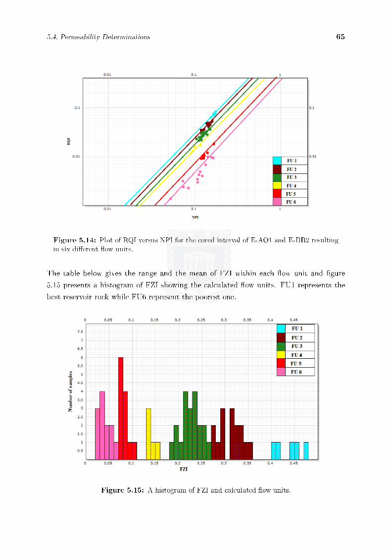
5.4. Permeability Determinations 65
Figure 5.14: Plot of RQI versus NPI for the cored interval of E-AO1 and E-BB2 resultingin six di�erent �ow units.
The table below gives the range and the mean of FZI within each �ow unit and �gure
5.15 presents a histogram of FZI showing the calculated �ow units. FU1 represents the
best reservoir rock while FU6 represent the poorest one.
Figure 5.15: A histogram of FZI and calculated �ow units.

5.4. Permeability Determinations 66
Table 5.6: The range and the mean of FZI within the calculated �ow units.
Flow Unit FZI Range Mean FZIFU 6 0-0.07 0.04FU 5 0.07-0.13 0.083FU 4 0.13-0.18 0.141FU 3 0.18-0.27 0.225FU 2 0.27-0.36 0.313FU 1 > 0.36 0.441
5.4.3.2 Estimation of Flow Units in Uncored Intervals and Wells
The method discussed in the previous section predicts the �ow units for the cored interval
of the studied wells. To extend the calculated �ow units in uncored interval and wells the
Ipsom module in Techlog is used. This module provides automatic classi�cation based on
the neural network technology as discussed in chapter four. Generally, this classi�cation
is an identi�cation of groups that are internally similar and di�erent from others in the
data according to indexation set.
To predict �ow units from wireline logs; �ve logs were used as input parameters. The
�ve are the: density log (RHOB), neutron log (NPHI), gamma ray log (GR), sonic log
(DT) and deep resistivity log (ILD/LLD). The core identi�ed �ow units were used as an
indexation set.
The obtained �ow units in E-AO1 and E-BB1 are shown in �gures 5.16 and 5.17 with the
core identi�ed �ow units for validation. The results obtained from the Ipsom classi�er
are in good match with the core identi�ed �ow units and can be used for permeability
calculations.

5.4. Permeability Determinations 67
Figure 5.16: Correlation between core �ow units and wireline �ow units in E-AO1.
Figure 5.17: Correlation between core �ow units and wireline �ow units in E-BB1.

5.4. Permeability Determinations 68
5.4.3.3 Permeability Prediction from Flow Units
The regression approach used to predict permeability in the previous section ignores the
e�ects of lithological sequence and physics of �ow at the pore scale within the cored
formation. Flow units o�er the opportunity to establish a relationship between formation
of similar �uid conductivity and petrophysical parameters.
The correlation of RQI versus FZI yields a R2 of 0.96 as shown in �gure 5.18.
Figure 5.18: The relationship between �ow zone indicator (FZI) and reservoir quality index(RQI) in the cored wells.
The regression equation is:
RQI = 0.2019 ∗ FZI − 0.0045 (5.16)
given that:
(RQI) = 0.0314√
K/Φ
Equation 5.16 can be written as:
0.0314√
K/Φ = 0.2019 ∗ FZI − 0.0045 (5.17)
The permeability then can be obtained as following:
K = (5.893 ∗ FZI − 0.1433)2 ∗ Φ (5.18)

5.4. Permeability Determinations 69
Equation 5.18 is used to calculate the permeability from wireline logs. The total porosity
model and the mean FZI presented in table 5.6 are used as inputs. Figures 5.19 and 5.20
show the predicted permeability of E-AO1 and E-BB1 plotted in track four together with
core permeability for validation. The calculated permeability is in a good match range
with core permeability and will be used as permeability model.
Figure 5.19: Comparison of core and log permeability models for Well E-AO1.

5.4. Permeability Determinations 70
Figure 5.20: Comparison of core and log permeability models for Well E-bb1.

Chapter 6
Determination of Cut-O� and Net Pay
This chapter discusses the �nal petrophysical results of the studied reservoirs. It includes
determinations of the net pay intervals within the 13 reservoirs identi�ed in the previous
chapters.
For any reservoir characterization; determination of net pay is needed to calculate volu-
metric hydrocarbons in place. Net pay is de�ned as any interval that contains producible
hydrocarbon at economic rates. Normally the net pay thickness is related to the reservoir
rock by the mean of net to gross ratio. The net to gross ratio is the ratio of the net pay
thickness to the total thickness of the studied reservoir. (Worthington and Consentino,
2005) showed that net pay and net to gross ratio are crucial to compute the hydrocarbon
reserves and have a signi�cant impact on the economic possibility of hydrocarbon reser-
voir production.
The gross interval for the studied wells was determined by consider the top and bottom
of the prede�ned reservoir zones.
6.1 Cut-O� Determinations
Net pay determination usually involves applying set of appropriate cut-o�s on petrophys-
ical parameter to distinguish between intervals that have reservoir potential, and intervals
that do not.
Historically, several approaches have tried to locate productive zones by comparing the
readings of di�erent wireline logs at a certain depth to classify the gross interval into net
pay and non-net pay intervals. These approaches include using of combination of gamma
and resistivity logs as proposed by (Snyder, 1971). Modern methods include using a
di�usivity equation to calculate net pay from wireline logs (Masoudi et al., 2011).
71

6.1. Cut-O� Determinations 72
In this study the conventional method to calculate the cut-o� has been used. This includes
applying cut-o� to permeability, porosity, shale volume and water saturation by making
use of core measurements to get reliable estimations.
6.1.0.4 Permeability Cut-O�
Permeability cut-o� is usually the starting point in net pay determinations (Cobb and
Marek, 1998). It is considered as the controlling parameter that directly separate reser-
voirs from non-reservoir rocks (Widarsono, 2010). Pores with permeability less than cut-
o� values will not allow �uids to �ow. In gas reservoirs, the permeability cut-o� should
be very low because gas is more mobile than oil.
In the studied wells the permeability cut-o� value is considered to be 0.1 mD. Core per-
meability is available for the two key wells (E-AO1 and E-BB1). Figure 6.1 shows the
core permeability histogram of these two wells showing the cut-o� points and the reservoir
and non-reservoir rocks.
Figure 6.1: Core permeability histogram of the key wells showing the cut-o� points.
6.1.0.5 Porosity Cut-O�
The determination of porosity cut-o� values relies on a generating porosity-permeability
relationship from the core measurement. A semi logarithmic porosity vs. permeability
cross-plot of the key wells is presented in �gure 6.2 below. The �gure indicates that a
porosity of 7 percent corresponds to the permeability cut-o� (0.1mD).

6.1. Cut-O� Determinations 73
Figure 6.2: Porosity-permeability cross plot to estimate porosity cut-o� values.
6.1.0.6 Shale Volume Cut-O�
The shale volume cut-o� is used to distinguish between reservoir and non- reservoir rock.
It de�nes the reservoir intervals by removing all intervals that have a volume of shale
more than a certain value of shale.
The volume of shale versus porosity with gamma-ray log used as a colour mode of the
studied wells is presented in �gure 6.3 below. A value of 0.35 is determined as the shale
volume cut-o�.

6.1. Cut-O� Determinations 74
(a) E-AD1 (b) E-AO1
(c) E-AO2
(d) E-BB1 (e) E-BB2
Figure 6.3: Volumes of shale versus porosity cross plots of the �ve studied wells showingthe reservoir and non-reservoir intervals
6.1.0.7 Water Saturation Cut-O�
To distinguish between the hydrocarbons pay zone and water zones; the saturation cut-
o� of the studied reservoirs is determined. Presented in �gure 6.4, the water saturation
of the studied reservoirs is cross plotted versus total porosity. A value of 60% is deter-
mined as water saturation cut-o�. Intervals that identi�ed as pay zone from porosity and
shale volume cut-o� must have values of water saturation less than 60% to consider as
hydrocarbons zones.
6.1. Cut-O� Determinations 75
(a) E-AD1 (b) E-AO1
(c) E-AO2
(d) E-BB1 (e) E-BB2
Figure 6.4: Water saturation versus porosity cross plots of the �ve studied wells showingthe reservoir and non-reservoir intervals.

6.2. Net Pay 76
6.2 Net Pay
This section determines, on the basis of prede�ned cut-o�s, the reservoir intervals and
thickness. The gross thickness is de�ned as the interval from the top to the bottom of the
reservoir zone including all non-reservoir rock. Within this interval, net interval de�nes
the thickness that contains producible hydrocarbon at an economic rate.
The calculated cut-o� values have been applied to studied reservoirs to determine the net
pay within each reservoir. The porosity cut-o� (0.07), shale volume cut-o� (0.35) and
water saturation cut-o� (0.6) are used for net pay calculation in this study. The non-net
pay intervals were excluded by using a minimum porosity cut-o�, maximum shale volume
and water saturation cut-o�. The obtained results are discussed further in this chapter.
6.2.1 E-AD1
As discussed in chapter four, E-AD1 has three reservoirs. The total gross thickness and net
pay thickness are 82.18 and 11.58 respectively. The obtained results are given in �gures
6.5, 6.6 and 6.7. 6.1 presents the calculated net pay summary for each reservoir with the
average bulk volume water, shale volume, porosity, water saturation and permeability.
The bulk volume water (BVW)is product of total porosity and water saturation.
Figure 6.5: Calculated reservoir parameters and net pay interval for reservoir one in E-AD1.

6.2. Net Pay 77
Figure 6.6: Calculated reservoir parameters and net pay interval for reservoir two in E-AD1.
Table 6.1: Summary of calculated reservoir pay parameters for E-AD1
Reservoir Top Bottom Gross Net Net/Gross BVW VSh Φ Sw KOne 2497.57 2527.81 30.24 4.42 0.146 0.324 0.204 0.138 0.53 4.311
Two 2529.21 2570.27 41.065 0 0 - - - - -Three 2827.84 2838.72 10.877 7.163 0.659 0.405 0.115 0.109 0.519 2.489

6.2. Net Pay 78
Figure 6.7: Calculated reservoir parameters and net pay interval for reservoir three inE-AD1.
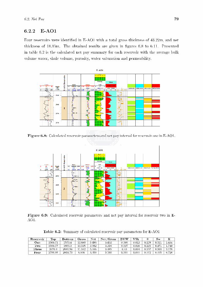
6.2. Net Pay 79
6.2.2 E-AO1
Four reservoirs were identi�ed in E-AO1 with a total gross thickness of 43.22m, and net
thickness of 18.35m. The obtained results are given in �gures 6.8 to 6.11. Presented
in table 6.2 is the calculated net pay summary for each reservoir with the average bulk
volume water, shale volume, porosity, water saturation and permeability.
Figure 6.8: Calculated reservoir parameters and net pay interval for reservoir one in E-AO1.
Figure 6.9: Calculated reservoir parameters and net pay interval for reservoir two in E-AO1.
Table 6.2: Summary of calculated reservoir pay parameters for E-AO1
Reservoir Top Bottom Gross Net Net/Gross BVW VSh Φ Sw KOne 2560.71 2573.4 12.689 5.486 0.432 0.366 0.012 0.128 0.521 1.434
Two 2590.77 2603.3 12.535 3.962 0.316 0.227 0.028 0.122 0.471 1.740
Three 2670.4 2681.56 11.162 5.446 0.488 0.43 0.004 0.157 0.503 3.176
Four 2796.89 2803.73 6.836 3.458 0.506 0.161 0.041 0.112 0.415 0.728

6.2. Net Pay 80
Figure 6.10: Calculated reservoir parameters and net pay interval for reservoir three inE-AO1.
Figure 6.11: Calculated reservoir parameters and net pay interval for reservoir four inE-AO1.
6.2.3 E-AO2
E-AO2 has two reservoirs, and both showed net pay potentials. The total gross thickness
and net pay thickness are 15.12m and 5.33m respectively. The obtained results are given
in �gure 6.12. Table 6.3 shows the calculated net pay summary for each reservoir with the
average bulk volume water, shale volume, porosity, water saturation and permeability.
Table 6.3: Summary of calculated reservoir pay parameters for E-AO2
Reservoir Top Bottom Gross Net Net/Gross BVW VSh Φ Sw KOne 2911.01 2921.3 10.29 2.591 0.252 0.132 0.066 0.105 0.483 5.273
Two 2923.64 2928.46 4.826 2.743 0.568 0.139 0.001 0.097 0.523 10.248

6.2. Net Pay 81
Figure 6.12: Calculated reservoir parameters and net pay interval for reservoir one andtwo in E-AO2.
6.2.4 E-BB1
Only one reservoir was identi�ed in E-BB1 with a total gross thickness of 29.19m, and
net thickness of 28.58m. The obtained results are given in �gure 6.13. Presented in table
6.4 is the calculated net pay summary for each reservoir with the average bulk volume
water, shale volume, porosity, water saturation and permeability.
Table 6.4: Summary of calculated reservoir pay parameters for E-BB1
Reservoir Top Bottom Gross Net Net/Gross BVW VSh Φ Sw KOne 2843.7 2872.89 29.193 28.583 0.979 1.116 0.074 0.112 0.35 15.399
6.2.5 E-BB2
Three reservoirs were identi�ed in E-BB1 with a total gross thickness of 49.28m, and net
thickness of 38.73m. The obtained results are given in �gures 6.14, 6.15 and 6.16. Shown
in table 6.5 is the calculated net pay summary for each reservoir with the average bulk
volume water, shale volume, porosity, water saturation and permeability.
Table 6.5: Summary of calculated reservoir pay parameters for E-BB2
Reservoir Top Bottom Gross Net Net/Gross BVW VSh Φ Sw KOne 2539.31 2550.59 11.279 7.925 0.703 0.377 0.064 0.114 0.415 2.594
Two 2577.43 2585.25 7.815 1.219 0.156 0.048 0.06 0.086 0.458 3.414
Three 2847.42 2877.6 30.186 29.592 0.98 0.922 0 0.114 0.273 12.561

6.2. Net Pay 82
Figure 6.13: Calculated reservoir parameters and net pay interval for reservoir four inE-BB1.
Figure 6.14: Calculated reservoir parameters and net pay interval for reservoir one inE-BB2.

6.2. Net Pay 83
Figure 6.15: Calculated reservoir parameters and net pay interval for reservoir two inE-BB2.
Figure 6.16: Calculated reservoir parameters and net pay interval for reservoir three inE-BB2.

Chapter 7
Conclusions and recommendations
7.1 Conclusions
In this research project; the petrophysical evaluation of 13A and 14A sequences in the
central Bredasdorp Basin was been carried out. The study investigated the reservoir units
encountered by �ve wells with insu�cient wireline logs and limited core data.
Four di�erent lithofacies were identi�ed from core data according to grain size and sed-
imentary structure. Facies A and B are recognized as reservoir rocks, whereas facies C
and D were considered as non-reservoir rocks. These lithofacies were used to predict the
electrofacies from wireline logs in uncored intervals. The classi�er used in this prediction
resulted in a good match with core facies.
The 13A and 14A sequences boundaries were identi�ed from wireline logs. The sequences
range falls between 2570m to 2928m depending on the position of the well. Multi-well
correlation between sequences was performed to link these sequences and determine trends
between the wells. A total of 13 reservoirs zones were isolated across the depth of the �ve
studied wells.
An integrated approach was used to predict the petrophysical parameters. The available
core data and wireline logs were comprehensively analyzed to determine shale volume,
porosity, water saturation and permeability. Core data was used to calibrate the petro-
physical model.
Six hydraulic �ow units were identi�ed in the studied reservoirs by making use of core
porosity and permeability. These core �ow units were used to predict �ow units from
wireline logs in uncored intervals. The studied reservoirs were the subject of permeability
predictions by hydraulic �ow units to consider the complex variation in pore geometry
within di�erent rock types.
84

7.2. Recommendations 85
Net pay determinations were conducted to distinguish between reservoir and non-reservoir
rocks. Cut-o� values of 7% for porosity, 35% for shale volume, and 60% water satura-
tion were used. The resulting distribution of these estimated petrophysical parameters
suggested that the central Bredasdorp Basin is a potential �eld for gas.
7.2 Recommendations
This petrophysical study could have been more e�cient with better quality wireline log
data, and more core measurements. Such data could improve log interpretation of the
Bredasdorp Basin.
A detailed study and petrophysical evaluation of water saturation is recommended to
establish a water saturation model for the Bredasdorp Basin.

References
Adeoti, L., Ayolabi, E., and James, P. (2009). An integrated approach to volume of shale analysis:
Niger delta example, orire �eld. World Applied Sciences Journal, 7(4):448�452.
A�fy, W. E. and Hassan, A. H. I. (2010). Permeability and porosity prediction from wireline
logs using neuro-fuzzy technique. Ozean Journal of Applied Sciences, 3(1):157�175.
Ahmed, U., Crary, S. F., Coates, G. R., et al. (1991). Permeability estimation: The various
sources and their interrelationships. Journal of Petroleum Technology, 43(05):578�587.
Al-Saddique, M. A., Hamada, G., and Al-Awad, M. N. (2000). Recent advances in coring and
core analysis technology new technique to improve reservoir evaluation. Engineering journal
of the University of Qatar, 13.
Alger, R. P. (1980). Geological use of wireline logs in development in petroleum geology. Applied
science publication London, 2 edition.
Amaefule, J. O., Altunbay, M., Tiab, D., Kersey, D. G., Keelan, D. K., et al. (1993). Enhanced
reservoir description: using core and log data to identify hydraulic (�ow) units and predict
permeability in uncored intervals/wells. Society of Petroleum Engineers, Annual Technical
Conference and Exhibition, pages 205�220.
Archie, G. E. (1942). The electrical resistivity log as an aid in determining some reservoir
characteristics. Petroleum Technology, pages 54�62.
Asquith, G. and krygowski, D. (2004). Basic well Log analysis for geologists. Number 16.
American Association of Petroleum Geologist, Tulsa, Oklahoma, USA.
Balan, B., Mohaghegh, S., and Ameri, S. (1995). State-of-the-art in permeability determination
from well log data: Part 1-a comparative study, model development. Society of Petroleum
Engineers, (30988).
Bassiouni, Z. (1994). Theory, Measurement, and interpretation of well logs, volume 4 of textbook
series. Society of Petroleum Engineers.
Benedictus, T. (2007). Determination of petrophysical properties from well logs of the o�shore
terschelling basin and southern central north sea graben region ( ncp-2a ) of the netherlands.
86

REFERENCES 87
Borhani, T. and Emadi, S. H. (2011). Application of hydraulic �ow units and intelligent systems
for permeability prediction in a carbonate reservoir. page 6.
Brown, L., Benson, J., Brink, G., Doherty, S., Jollands, A., Jungslager, E., Keenan, J., Munt-
ingh, A., and Van Wyk, N. (1995). Sequence Stratigraphy in O�shore South African Divergent
Basins: An Atlas on Exploration for Cretaceous Lowstand Traps by Soekor (Pty) Ltd. Num-
ber 41. American Association of Petroleum Geologists.
Burden, P. (1992). Soekor, partners explore possibilities in bredasdorp basin o� south africa. Oil
and Gas Journal, pages 109�115.
Burden, P. and Davies, C. (1997). Exploration to �rst production on block 9 o� south africa.
Oil and Gas Journal, 1(92-98.).
Catuneanu, O., Abreu, V., Bhattacharya, J. P., Blum, M., Dalrymple, R., Eriksson, P., Fielding,
C., Fisher, W., Galloway, W., Gibling, M., Giles, K., Holbrook, J., Jordan, R., Kendall, C.,
Macurda, B., Martinsen, O., Miall, A., Neal, J., Nummedal, D., Pomar, L., Posamentier, H.,
Pratt, B., Sarg, J., Shanley, K., Steel, R., Strasser, A., Tucker, M., and Winker, C. (2009).
Towards the standardization of sequence stratigraphy. Earth-Science Reviews, 92:1�33.
Clavier, Huyle, W., and D., M. (1971). Quantitative interpretation of t.d.t logs; part i and ii.
Journal of Petroleum Technology, 23(6):743�763.
Clu�, S. and Clu�, R. (2004). Petrophysics of the lance sandstone reservoirs in jonah �eld,
sublette county, wyoming. in Jonah Field: Case Study of a Giant Tight-Gas Fluvial Reservoir
American Association of Petroleum Geologists: Studies in Geology, 52.
Cobb, W. and Marek, F. (1998). Net pay determination and water�ood depletion mechanisms.
Society of Petroleum Engineers 48952, in the Annual Technical Conference and Exhibition.
De Wit, M. J. and Ransome, I. G. (1992). Regional inversion tectonics along the southern
margin of gondwana. Inversion tectonics of the Cape Fold Belt, Karoo and Cretaceous basins
of southern Africa, pages 15�21.
Ebanks, W. J., Scheihing, M., and Atkinson, C. (1993). Flow units for reservoir characteriza-
tion. Development geology reference manual: American Association of Petroleum Geologists:
Methods in Exploration Series, 10:282�285.
Ellis, D. and Singer, J. (2008). Well Logging for Earth Scientists. Springer, second edition
netherlands edition.
Enikanselu, P. and Adekanle, A. (2008). A fortran programme for computing formation ( connate
) water resistivity from spontaneous potential logs. American-Eurasian Journal of Scienti�c
Research, 3(2):172�177.

REFERENCES 88
Fuad, M. Q. (2008). Formation Evaluation of Upper Qamchuqa Reservoir, Khabbaz Oil Field,
Kirkuk Area, Northeastern Iraq. PhD thesis, University of Sulaimani.
Galford, J., Flaum, C., Gilchrist Jr., W., Soran, P., and Gardner, J. (1988). Improved environ-
mental corrections for compensated neutron logs. Society of Petroleum Engineers, 3, Number
2:371�376.
Gluyas, J. and Swarbick, R. (2004). Petroleum geoscience. Oxford: Blackwell Publishing Co.
Gunter, G., Pinch, J., Finneran, J. M., and Bryant, W. T. (1997). Overview of an integrated
process model to develop petrophysical based reservoir descriptions. Society of Petroleum
Engineers, (38748).
Hamada, G. and Abushanab, M. (2008). Better porosity estimate of gas sandstone reservoirs
using density and nmr logging data. Emirates Journal for Engineering Research, 13(3):47�54.
Kamel., M. H. and Mabrouk., W. M. (2003). Estimation of shale volume using a combination of
the three porosity logs. Journal of Petroleum Science and Engineering, 40:145�157.
Krygowski, D. A. (2003). Guide to Petrophysical Interpretation. Austin Texas U.S.A.
Lehmann, K. (2010). Environmental corrections to gamma-ray log data: Strategies for geophys-
ical logging with geological and technical drilling. Journal of Applied Geophysics, 70:17�26.
Liro, L. M. and Dawson, W. C. (2000). Reservoir systems of selected basins of the south atlantic.
in: Mello M.R. and Katz B.J. (eds.), Petroleum system of South Atlantic margins: American
Association of Petroleum Geologists Memoir, 73:77�92.
Masoudi, P., Tokhmechi, B., Zahedi, A., and M., A. J. (2011). Developing a method for identi�ca-
tion of net zones using log data and di�usivity equation. Journal of Mining and Environment,
2(1):53�60.
McLachlan, I. and McMillan, I. (1976). Review and stratigraphic signi�cance of southern cape
mesozoic palaeontology. Transactions of the Geologic Society of South Africa, 79(197-212).
McMillan, I., Brink, G., Broad, D., and Maier, J. (1997). Late mesozoic sedimentary basins o�
the south coast of south africa. Sedimentary Basins of the World, 3:319�376.
Mitchum, R., Vail, P., Todd, R., Widmier, J., Thompson, S., Sangree, J., Bubb, J., and W.G, H.
(1977). Seismic stratigraphy and changes of sea-level, part 1: Glossary of terms used in seismic
stratigraphy. In: Payton, C.E. (eds.), Seismic stratigraphy and application to hydrocarbon
exploration. American Association of Petroleum Geologists Memoir, 26:205�212.
Moake, G. (2008). An accelerometer- and tension-based depth correction suitable for image logs.
Society of Petrophysicists and Well-Log Analysts, 2008-UU.

REFERENCES 89
Nooruddin, H. A. and Hossain, M. E. (2011). Modi�ed kozeny-carmen correlation for enhanced
hydraulic �ow unit characterization. Journal of Petroleum Science and Engineering, 80(1):107�
115.
Octavian, C. (2006). Principles of Sequence Stratigraphy. Elsevier, �rst edition.
Opuwari, M. (2010). Petrophsical Evaluation of The Albian Age Gas Bearing Sandstone Reservoir
of the O-M Field, Orange basin, South Africa. PhD thesis, University of the Western Cape.
PASA (2003). Petroleum exploration information and opportunities: Petroleum agency of south
africa brochure.
PASA (2004/2005). Petroleum exploration information and opportunities: Petroleum agency of
south africa brochure.
PASA (2008). Petroleum exploration information and opportunities: Petroleum agency of south
africa brochure.
Poupon, A. and Leveaux, J. (1971). Evaluation of water saturation in shaly formations. Society
of Petrophysicists and Well Log Analysts. 12th Annual Logging Symposium.
Qi, L. and Carr, T. (2006). Neural network prediction of carbonate lithofacies from well logs, big
bow and sand arroyo creek �elds, southwest kansas. Computers and Geosciences, 32:947�964.
Raymer, L., Hunt, E., and Gardner, J. (1980). An improved sonic transit time-to-porosity
transform. Society of Petrophysicists and Well Log Analysts. 21 Ann. Logging Symposium.
Rider, M. (1996). The geological Interpretation of well logs. Rider-French consulting LTD, second
edition.
Schalkwyk, H. J.-M. (2005). Assessment controls on reservoir performance and the a�ects of
granulation seam mechanics in the bredasdorp basin, south africa. Master's thesis, Uniersity
of the Western Cape.
Schlager, W. (1999). Type 3 sequence boundaries. In: Harris, P, Saller, A. and Simo, A. (eds),
Carbonate sequence stratigraphy: application to reservoirs, outcrops and models. Society of
Sedimentary Geology, Spec. Pub. 63, p. 35-46.
Schlumberger (1989). Log Interpretation Charts. Schlumberger Oil�eld Services, Houston.
Selley, R. (2000). Applied Sedimentology. Academic Press, San Diego, California, USA., second
edition.
Snyder, R. (1971). A review of the concepts and methodology of determining "net pay". in Fall
Meeting of the Society of Petroleum Engineers of AIME1971, New Orleans, Louisiana.

REFERENCES 90
Soto, B. R., Arteaga, D., Hidalgo, C. M., and Rodriguez, F. (2010). Correct shale-volume char-
acterization increases hydrocarbon reserves: Case study of cretaceous formation lake of mara-
caibo venezuela. In Society of Petroleum Engineers Latin American and Caribbean Petroleum
Engineering Conference. Society of Petroleum Engineers, (136811).
Steiber, R. (1973). Optimization of shale volumes in open hole logs. Journal of Petroleum
Technology, 31:147�162.
Tang, H. and White, C. (2008). Multivariate statistical log log-facies classi�cation on a shallow
marine reservoir. Petroleum Science and Engineering, 61:88�93.
Thomson, K. (1998). When did the falklands rotate? Marine and petroleum geology, 15(8):723�
736.
Tinker, J., de Wit, M., and Brown, R. (2008). Linking source and sink: evaluating the balance
between onshore erosion and o�shore sediment accumulation since gondwana break-up, south
africa. Tectonophysics, 455(1):94�103.
Ushie, F. (2001). Formation water resistivity (rw) determination: the sp method. Applied
Environmental Manage, 3:172�177.
Widarsono, B. (2010). Single or multiple porosity cut-o�? a new relevange provided by applica-
tion of a new approach. LEMIGAS Scienti�c Contribution, 33(1):1�8.
Worthington, P. (1991). E�ective integration of core and log data. Society of Core Analysis,
(9102).
Worthington, P. and Consentino, L. (2005). The role of cut-o�s in integrated reservoir studies.
Society of Petroleum Engineers Reservoir: Evaluation and Engineering, 8(4):276�290.
Yumei, L. (2006). Facies identi�cation from well logs : A comparison of discriminant analysis
and naive bayes classi�er. Petroleum Science and Engineering, 53:149�157.
Zee Ma, Y. (2011). Lithofacies clustering using principal component analysis and neural network:
Applications to wireline logs. Mathematical Geosciences, 43(4):401�419.

Appendices
Appendix A
Well E-BB1 core analysis results
Depth Φ K K Air Gas Oil Water Grain Density
M % md md % % % g/cm32846.05 13.8 29.05 26.29 70 5 25 2.672846.25 11.7 14.56 12.95 2.662846.54 13.1 30.06 27.66 2.652846.79 13.1 32.17 29.29 2.652847.05 13 25.94 23.56 66 4 30 2.662847.25 10.1 5.67 4.82 2.652847.5 11.2 13.88 12.41 2.652847.75 11.5 12.11 10.65 2.652848.03 11.2 10.34 9.04 67 5 28 2.652848.25 13.1 27.47 24.83 2.642848.5 13.2 27.25 24.87 2.652848.75 13.8 28.4 25.79 2.672849.05 12.6 30.47 28.11 67 0 33 2.652849.27 14.4 42.73 39.29 2.652849.53 8.9 1.4 1.01 2.662849.78 9.3 1.74 1.3 2.662850.05 12 16.1 14.44 67 4 29 2.652850.25 13.3 29.95 27.49 2.652850.47 13.3 22.31 20.03 2.652850.72 10.7 5.12 4.27 2.652851.05 11.9 9.04 7.78 66 5 29 2.662851.22 11.3 7.7 6.5 2.652851.46 13.5 20.22 18.19 2.662851.72 13.4 17.83 15.81 2.652852.03 8.4 0.21 0.1 47 19 34 2.672852.29 9 0.89 0.61 2.652852.79 12.8 14.33 12.56 2.652853.11 13.8 18.48 16.7 73 0 27 2.68
91

92
Depth Φ K K Air Gas Oil Water Grain Density
M % md md % % % g/cm32853.33 12.2 12.12 10.62 2.652853.58 11.5 8.19 7.04 2.662853.83 11.8 10.33 9 2.652854.05 12.5 11.36 9.91 65 4 31 2.672854.22 12 12.01 10.49 2.652854.51 9.3 1.72 1.25 2.652854.76 9.7 2.56 1.97 2.642855.05 11.3 5.64 4.68 66 5 29 2.662855.22 11.4 7.31 6.15 2.652855.47 10.8 6.97 5.87 2.642855.72 12.5 11.28 9.7 2.682856.05 11.1 3.38 2.65 62 8 30 2.672872.05 11.9 18.08 16.45 46 15 39 2.652872.27 9.6 3.55 2.88 2.652872.57 0.3 0.03 0.02 2.66

93
Appendix B
Well E-AO1 core analysis results
Depth Φ Corrected Φ K Corrected K Water Oil Gas Grain Density
M % % md md % % % g/cm3
2674.05 16.1 15.7 111.57 104.8 84 0 16 2.732674.3 15.5 14.9 109.31 103.48 2.682674.55 15.9 14.4 77.11 72.75 2.672674.8 15.3 14.8 96.83 91.54 2.682675.05 14.6 14.2 88 82.99 89 0 11 2.682675.25 13.8 13.3 55.89 52.74 2.692675.5 14 13.5 37.13 35.15 2.692675.75 12.7 12.3 10.22 9.6 2.72675.9 14.8 14.3 5.19 4.81 63 0 37 2.72676.2 14.2 13.5 1.56 1.29 2.682676.45 11.9 11.3 1.61 1.38 2.672676.7 12.9 12.3 2.15 1.8 2.672676.96 14.7 14.1 1.62 1.25 67 0 33 2.682677.3 10.4 9.8 0.16 0.09 2.662677.55 12.4 11.8 0.69 0.57 2.682677.8 12 11.5 1.63 1.32 2.682677.97 12.9 12.4 1.64 1.25 59 0 41 2.692678.25 11.8 10.9 0.33 0.18 2.682678.5 12 11.3 1.36 1 2.682678.75 5.5 5 0.04 0.01 2.722678.93 11.1 10.6 1.18 0.9 56 0 44 2.72679.15 11.7 11.1 1.32 1.08 2.682679.4 11.7 11.2 1.21 0.97 2.672679.65 11.9 11.3 1.35 1.1 2.672679.89 11.5 11.1 1.36 1.16 49 0 51 2.672680.2 10.6 10.1 0.28 0.19 2.672680.45 10.7 10.4 0.36 0.26 2.682680.7 10.4 9.7 0.19 0.12 2.692680.89 7.3 6.8 0.12 0.07 48 0 52 2.682681.15 7.5 6.9 0.08 0.04 2.68

94
Appendix C
Uncorrected Porosity and Corrected Porosity in E-BB1
Depth Uncorrected Porosity Corrected Porosity
M % %
2846.05 13.8 13.156642846.25 11.7 11.076512846.54 13.1 12.463262846.79 13.1 12.463262847.05 13 12.364212847.25 10.1 9.4916482847.5 11.2 10.581242847.75 11.5 10.87842848.03 11.2 10.581242848.25 13.1 12.463262848.5 13.2 12.562322848.75 13.8 13.156642849.05 12.6 11.967992849.27 14.4 13.750962849.53 8.9 8.3030022849.78 9.3 8.6992172850.05 12 11.373672850.25 13.3 12.661372850.47 13.3 12.661372850.72 10.7 10.085972851.05 11.9 11.274622851.22 11.3 10.680292851.46 13.5 12.859482851.72 13.4 12.760432852.03 8.4 7.8077332852.29 9 8.4020562852.79 12.8 12.16612853.11 13.8 13.156642853.33 12.2 11.571782853.58 11.5 10.87842853.83 11.8 11.175562854.05 12.5 11.868942854.22 12 11.373672854.51 9.3 8.6992172854.76 9.7 9.0954332855.05 11.3 10.680292855.22 11.4 10.779352855.47 10.8 10.185032855.72 12.5 11.868942856.05 11.1 10.48219