WATER QUALITY RESEARCH PROGRAM

S AMISCELLANEOUS PAPER E-89-1

FORMULATION OF WATER,QUALITY MODELS00 FOR STREAMS, LAKES, AND RESERVOIRS,

MODELER'S PERSPECTIVEby

U Heinz G. Stefan

S ... St. Anthony Falls Hydraulic LaboratoryUniversity of Minnesota

Minneapolis. Minnesota 55414

Robert .,. Ambrose, Jr.

Environmental Research LaboratoryUS Environmental Protection Agency

Athens, Georgia 30613

and

Mark S. Dortch

Environmental Laboralor

rWW, DEPARTMENT OF THE ARMYWaterways Experiment Station, Corps of Engineers

- , PO Box 631, Vicksburg, Mississippi 39181-0631

SMLELEC TEDOWAi¢ "-.- ~AUG 10 1989 /[ € ,.

Jilly 1989)

S9, 8 O9 0O13

Destroy this report when no longer needed. Do not returnit to the originatcr.

The findings in this report are not to be construed as an officialDepartment of the Army position unless so designated

by other authorized documents.

The contents of this report are not to be used foradvertising, publication, or promotional purposes.Citation of trade names does not constitute an

official endorsement or approval of the use ofsuch commercial products.

Unclassified

SECURITY CLASSIFICATION OF THIS PAGE

form ApprovedREPORT DOCUMENTATION PAGE OMBNo 0 704 1e8

Exp Date Jun 30 7986la REPORT SECURITY CLASSIFICATION lb RESTRICTIVE MARKINGSUnclassified

2a SECURITY CLASSIFICATION AUTHORITY 3 DISTRIBUTION /AVAILABILITY OF REPORT

Approved for public release; distribution2b DECLASSIFICATION / DOWNGRADING SCHEDULE unlimited.

4 PERFORMING ORGANIZATION REPORT NUMBER(S) S MONITORING ORGANIZATION REPORT NUMBER(S)

Miscellaneous Paper E-89-1

6a NAME OF PERFORMING ORGANIZATION 66 OFFICE SYMBOL 7

a NAME OF MONITORING ORGANIZATION

See reverse. (If applicable)

6c. ADDRESS (City, State, and ZIPCode) 7b ADDRESS(City, State, and ZIP Code)

See reverse.

Ba. NAME OF FUNDING/SPONSORING T18b OFFfCF SYMBOL 9 PROCUREMENT !NSTRUMENT IDENTIFICATION NUMBERORGANIZATION (if app '.cable)US Army Corps of Engineers

8c. ADDRESS (City, State, and ZIP Code) 10 SOURCE OF FUNDING NUMBERS

PROGRAM PROJECT fTASK IWORK UNIT

Washington, DC 20314-1000 ELEMENT NO NO NO jACCESSION NO

11 TITLE (Include Security Classification)

Formulation of Watpr Quality Models for Streams, Lakes, and Reservoirs: Modeler'sPerspective

12 JER.ONAL AUTHOR( .Stetan, Heinz u.; Ambrose, Robert B., Jr.; Dortch, Mark S.

13a TYPE OF REPORT 13b TIME COVERED 14 DATE OF REPORT (Year, Month, Day) 15 PAGE COUNT

Final report FROM TO July 1989 8216 SUPPLEMENTARY NOTATION

Available from National Technical Information Service, 5285 Port Royal Road, Springfield,VA 22161.

17 COSATI CODES 18 SUBJECT TERMS (Continue on reverse if necessary and identify by block number)

FIELD GROUP SUB-GROUP Lakes StreamsNumerical models Water qualityReservoir

79 ABSTRACT (Continue on reverse if necessary and identify by block number)

An overview of process descriptions, assumptions, constraints, and other considera-tions that enter into the development of deterministic mathematical surface water qualitymodels is given in this report. Modeling of hydrodynamic transport is treated separatelyfor "standing" waters (lakes, reservoirs, ponds, and impoundments) and flowing waters(rivers and streams). Some information on sediment transport as it relates to waterquality is presented. Models addressing organic wastes and nutrients, synthetic organicchemicals, and metals transport and transformation are addressed in separate sections.The review ends with an outlook towards challenges and possible future developments.

20 DISTRIBUTION I AVAILABILITY OF ABSTRACT 21 ABSTRACT SECURITY CLASSIFICATION

0(UJNCLASSIFIEDfUNLMITED El SAME AS RPT 0 DTIC USERS Unclassified

22a NAME OF RESPONSIBLE INDIVIDUAL 22b TELEPHONE (Include Area Code) 22c OFFICE SYMBOL

DO FOPM 1473, 84 MAR R3 APR ed,tlon may be used until exhausted SECURITY CLASSIFICATION OF THIS PAGEAll other editions are oDsoiete Unc_ass eiT_

UnclassifiedSECURITY CLASSIFICATION OF THIS PAGE

6a and c. NAME AND ADDRESS OF PERFORMING ORGANIZATION (Continued).

University of Minnesota

St. Anthony Falls Hydraulic LaboratoryMinneapolis, MN 55414;

US Environmental Protection Agency

Environmental Research Laboratory

Athens, GA 30613;

USAEWES

Environmental Laboratory

PO Box 631, Vicksburg, MS 39181-0631

Unclassified

SECURITY CLASSIFICATION OF THIS PAGE

PREFACE

This report was published under the Water Quality Research Program

(WQRP), which is sponsored by the Headquarters, US Army Corps of Engineers

(HQUSACE), and is assigned to the US Army Engineer Waterways Experiment

Station (WES), under the purview of the Environmental Laboratory (EL). The

WQRP is managed under the Environmental Resources Research and Assistance

Programs (ERRAP). The HQUSACE Technical Monitor of WQRP is Mr. David P.

Buelow. Mr. J. Lewis Decell, WES, is the Program Manager of ERRAP.

This report was originally written as a paper for the International

Symposium on Water Quality Modeling of Agricultural Non-Point Sources, which

was held at Utah State University, Logan, UT, on 19-23 June 1988. The paper

was published as this report to make the information more available to Corps

of Engineers offices and others. The authors are Dr. Heinz G. Stefan, Depart-

ment of Civil and Mineral Engineering, St. Anthony Falls Hydraulic Laboratory,

University of Minnesota, Minneapolis, MN; Mr. Robert B. Ambrose, Jr., Environ-

mental Research Laboratory, US Environmental Protection Agency, Athens, GA;

and Mr. Mark S. Dortch, Chief, Water Quality Modeling Group, Ecosystem

Research and Simulation Division, EL, WES. This report was edited by

Ms. Lee T. Byrne of the WES Information Technology Laboratory.

Commander and Director of WES was COL Dwayne G. Lee, EN. Technical

Director was Dr. Robert W. Whalin.

This report should be cited as follows:

Stefan, Heinz G.; Ambrose, Robert B., Jr.; and Dortch, Mark S. 1989.

"Formulation of Water Quality Models for Streams, Lakes, and Reservoirs:Modeler's Perspective," Miscellaneous Paper E-89-1, US Army EngineerWaterways Experiment Station, Vicksburg, MS.

-I,

ATI 'c I

CONTENTS

Page

PREFACE..................................................................... 1

PART I: CONCEPTS OF SURFACE WATER QUALITY MODELING ..................... 3

Categories........................................................... 3Approach............................................................. 4

PART II: WATER QUALITY MODELS FOR STANDING WATERS(RESERVOIRS, PONDS, AND LAKES)................................. 8

Approaches........................................................... 8Zero-Dimensional Models of Reservoirs, Ponds,

and Lakes.......................................................... 11One-Dimensional Models of Reservoirs, Ponds, and Lakes ............... 13Two-Dimensional Models of Reservoirs, Ponds,

and Lakes.......................................................... 20Three-Dimensional Models of Reservoirs,

Ponds, and Lakes................................................... 22

PART III: WATER QUALITY MODELS FOR FLOWING

WATER (STREAMS AND RIVERS).................................... 26

Approaches........................................................... 26Analytical an. Numerical Steady-StateModels of Stream and River Water Quality.......................... 27

Dynamic Models of Stream and RiverWater Quality...................................................... 28

Inputs and Mixing Zones............................................. 29

Part IV: SEDIMENT TRANSPORT AND SEDIMENT/WATER QUALITYINTERACTIONS................................................... 32

Concepts............................................................. 32Processes............................................................ 32Model Formulations................................................... 35Examples of One-, Two-, and Three-

Dimensional Sediment Transport Models............................. 36

PART V: MODELS ADDRESSING ORGANIC WASTES ANDNUTRIENTS...................................................... 39

Concepts............................................................. 39Fate Processes....................................................... 39Simulation Models.................................................... 46

PART VI: SYNTHETIC ORGANIC CHEMICALS................................... 49

Fate Processes....................................................... 49Simulation Models.................................................... 55

PART VII: METALS......................................................... 59

Fate Processes....................................................... 59Simulation Models.................................................... 61

PART VIII: CHALLENGES AND RECOMMENDATIONS................................ 63

REFERENCES................................................................. 67

2

FORMULATION OF WATER QUALITY MODELS FOR STREAMS, LAKES, AND

RESERVOIRS: MODELER'S PERSPECTIVE

PART I: CONCEPTS OF SURFACE WATER QUALITY MODELING

Categories

1. Surface water quality (WQ) models can be categorized in various

ways. One is with reference to their formulation. On that basis, models may

be classified by the following distinctions:

a. Physical versus mathematical/numerical.

b. Mechanistic versus empirical.

c. Deterministic versus stochastic.

d. Steady-state versus unsteady.

e. Dimensionality (0, one-dimensional (1-D), two-aimensional (2-D),and three dimensional (3-D)).

f. Hydrodynamic assumptions.

&. Biogeochemical formulations.

This-paper deals with only mathematical/numerical, mechanistic, deterministic

surface WQ models. Compilations of available operational surface water models

including those that deal with water quality have been given at various times

by various organizations in the United States, e.g. by (a) Hydrologic Engi-

neering Center, US Army Corps of Engineers, Davis, CA (1987); (b) US Geologi-

cal Survey (USGS) (Jennings and Yotsokura 1980); (c) Office of Technology

Assessment, US Congress (1982); (d) US Environmental Protection Agency

(USEPA), Center for Water Quality Modeling (1980), Athens, GA; and (e) US Army

Engineer Waterways Experiment Station, Vicksburg, MS (1987).

2. The state of toxicant modeling in surface water was reviewed in 1979

(USEPA 1980); Figure I shows an example of the systems used. There have been

no substantive changes in the concept and/or dimensionality of the models,

but the number of recognized pollutant materials and interacting transforma-

tions has increased dramatically.

3

SIOMA SS TOXICANT

TOP TOXICANTTOP IN TOP

CARNIVORE CARNIVORE

~TOXICANT

ZOOPLANKTON INZOOPLANKTONI I

YTEM PHYTOPLANKTONSYSTEM

IPHYTOPLANKTON

TOXICANT TOXICANTNUTRIENT DISSOLVED IN j

SYSTEM IN WATER PARTICLES

______tWA TEN

S0/MENN

NUTRIENT OISSOLVED PARTICULATEDSYSTEM TOXICANT TOXICANT

Figure 1. Systems in toxicant WQ models (from UJSEPA (1980))

Approach

3. The classical approach to mechanistic model formulation is to sub-

divide each water body into a suitable number of control volumes. "Suitable"

depends on the purpose of the modeling effort, the shape and size of the water

body, and especially the time scale (years, months, weeks, days, or even

hours) to be modeled. The time scale influences the choice of physical trans-

port and chemical and biological transformation processes to be included in

the model. This selection process is presently more an art than a science.

4

One rule of thumb is that the shorter the time scale and the larger and more

complicated the geometry, the more control volumes will be required. Another

rule is to select the longest possible time scale because averaging over long

times often makes the model easier. Science takes over when the basic equa-

tions for each control volume are formulated. These equations are transport

(conservation) equations for mass of water and transport/transformation equa-

tions for materials in the water. The latter may include expressions for

energy transfer and expressions for chemical equilibrium or chemical and bio-

logical kinetics. Water quality parameters that have been modeled include:

a. Total dissolved solids (TDS), inorganic salts.

b. Inorganic suspended sediments (SS).

c. Temperature (T).

d. Organic wastes and dissolved oxygen (DO) (biochemical oxygendemand (BOD)).

e. Bacteria (Ecoli).

f. Nutrients (phosphorus, nitrogen, silicon).

a. Inorganic carbon (carbon (C), pH).

h. Biomass and food chains (chlorophyll a (Chl a), C, zooplankton,etc.).

i. Metals (lead, mercury, cadmium).

j_. Synthetic organic chemicals (polychlorinated biphenyls (PCBs)).

k. Radioactive materials (radium, plutonium).

I. Xrbicides, insecticides (Dieldrin, dichlorodiphenyltrichloro-

ethane (DDT)).

The classical formulations for nutrient uptake, growth (including photosynthe-

sis), predation, and microbial decomposition are widely used. Recent needs

are for models of toxic materials in the form of metals such qp mercury, lead,

and cadmium; organics such as PCBs; herbicides; and insecticides and for

models simulating lowered pH values caused by acid rain.

4. Since it is possible to produce a nearly infinite number of equa-

tions, the question to be answered by the modeler is not "how many equations

can I write" but "how many need to be written to solve the problem at hand."

The ideal model is the one with the smallest number of equations that can

solve the problem.

5. All models are formulated for a particular purpose. There is no

all-purpose model, and it is unlikely that one will ever be developed. Some

models may serve several purposes. It was the consensus of the participants

in a 1979 USEPA workshop (USEPA 1980, Thomann 1982) that the formulation of a

surface WQ model requires the interaction of three types of people:

(a) managers who recognize a WQ problem, (b) specialists who understand or are

capable of studying the processes which relate to the problems at hand, and

(c) modelers who can synthesize all information pertaining to the problem in

mathematical form and solve the resulting mathematical relationships. Only in

very simple cases may one person be able to fulfill all three roles.

6. General steps by which a surface WQ model is developed and put to

use are:

a. Specification of problems, issues, and objectives.

b. Specification of theoretical concepts and mathematical relation-ships (model selection).

c. Quantitative specifications of parameters/coefficients andboundary conditions.

d. Model calibration.

e. Model verification.

f. Determination of model sensitivity, accuracy, and uncertainty.

&. Application.

To this list, a No. 8 postapplication model audit should be added (Thomann and

Mueller 1987).

7. Conferences on WQ modeling have dealt with eutrophication (Federal

Water Pollution Control Administration (FWPCA) 1969, Lorenzen 1981), DeGray

lake (Kennedy and Nix 1987), general issues (Ott 1976, Nix and Black 1987),

toxic substances (Jorgensen 1984), and ecological modeling (Jorgensen 1979a).

8. Parameter values for WQ models must often be developed through field

and laboratory studies. Initin! estimates may be found in handbooks (e.g.

Jorgensen 1979b). Data sets that can be used for model calibration and veri-

fication are usually assembled on a case-by-case basis. A compilation for

four rivers, two lakes, and one estuary was given by Huber, MacIntyre, and

Heavey (1984).

9. In the following sections, some concepts and accomplishments of WQ

modeling are presented. Specifically the following are addressed:

(a) hydrodynamic transport in standing and flowing waters, (b) suspended sedi-

ment transport modeling and sediment/WQ interactions, (c) modeling of organic

wastes nutrients and eutrophication, and (d) modeling of toxic material

6

transport .,d transformation including synthetic organics (pesticides,

insectLA,.des) and metals. The report concludes with a list of some challenges

for the future as perceived by the authors.

7

PART II: WATER QUALITY MODELS FOR STANDING WATERS

(RESERVOIRS, PONDS, AND LAKES)

Approaches

10. The features and characteristics of reservoir, lake, or pond WQ

models are directly related to the peculiar thermo-hydrodynamics in such water

bodies, which make them substantially different from streams and rivers. In

rivers and streams, gravity is the main driving force, and bed friction is the

main resisting force, resulting in usually very perceptible velocities and

strong tendenc;/ to turbulent mixing. Lakes, ponds, and reservoirs are often

characterized by water movements that are very slow and weak. The driving

forces are from wind shear, solar radiation, heat exchange, and inflows and

outflows. Very small density differences caused by temperature gradients from

surface heating/cooling and/or by gradients in dissolved or suspended sub-

stances (salinity gradients, turbidity) often control the thermo-hydrodynamics

of standing waters. Phenomena that are usually absent or can be ignored in

river and stream flow analysis are dominant in "standing" waters, e.g., stable

temperature stratification that hinders vertical turbulent mixing; natural

convection caused by unstable density stratification; wind-driven circulation

and vertical mixing; density and turbidity currents; and selective withdrawal

from density-stratified water. The reader can find overviews of the hydro-

dynamic features of lakes, reservoirs, impoundments, and ponds in summaries by

Mortimer (1974), Wetzel (1975), Gibbs and Shaw (1977), Lerman (1978), Graf and

Mortimer (1979), Imberger (1979), Csanady k1980), Stefan (1981), Harleman

(1982), Imberger and Hamblin (1982), Henderson-Sellers (1984), Shanahan and

Harleman (1984), and Annandale (1987).

11. Hydrodynamics are the basis for many significant differences in

ecosystems of lakes/reservoirs and rivers/streams. Lakes that often have the

longest residence times of water (defined here as total volume of lake divided

by total outflow) develop seasonal successions of organisms and chemical pro-

cesses not affected by the swift motion found in rivers and streams. Storage

reservoirs can differ from lakes because of the dominant effects of water

level fluctuations and inflow. River impoundments created to make waterways

navigable may have fairly constant water levels but highly variable residence

8

time making them "typical" lakes at low flows and "typical" rivers at high

flows.

12. The interactions with the bed also are very different in flowing

and standing waters. Slow deposition of fine and organic material on lake/

reservoir beds can have a significant effect on water quality. Equally impor-

tant can be the release of materials (remineralized substances) from the bed

due to chemical processes or bacterial decomposition. Bioturbation by inver-

tebrates, fishes, etc., or wind-driven resuspension can contribute greatly to

WQ deterioration. In rivers the contributions of such processes are often

negligible compared with advective transport of water quality.

13. Water quality models of lakes, reservoirs, ponds and impoundments

can be formulated as zero-, one-, two- or three-dimensional (O-D, I-D, 2-D, or

3-D) in space (Figure 2). A O-D model will average concentration over the

entire water body without allowing variation in space; it will use only one

control volume for the entire lake or pond. A I-D model for standing water

usually includes the vertical dimension to account for stratification; thus

the model uses a series of horizontal layers. The 2-D models for standing

waters are either longitudinal-vertical for density stratified waters or depth

integrated in nonstratified, shallow waters of large horizontal dimensions.

In longitudinal-vertical coordinate systems, concentrations are given as

C(x,z) where x can be a longitudinal coordinate of a reservoir and z a

depth coordinate. Variations in concentration across the width are not

treated in such a model, and concentrations are assumed averaged with width

y . Such a model will require the use of control volumes stacked with depth

and length.

14. Selection of the lowest possible dimensionality, i.e. the smallest

number of control volumes (CV) is the most advantageous since a conservation

equation must be written for each CV and each WQ constituent. Selection of

the dimensionality of a lake, reservoir, pond, or impoundment WQ model may be

thought to depend mostly on the size of the water body, but it has been shown

to be ;- .Ily a function of the purpose of the model. The North American Great

Lake- r example, have been modeled very successfully as completely mixed

O-D conrin,')us flow reactors to develop phosphorous management strategies for

eut.ophicdtion control (Chapra 1977, Chapra and Reckhow 1983). Lake/reservoir

WQ models of different dimensionalities are discussed in the following

sections.

9

CONTROLVOLUME

0-D C(t)MIXED CELL

CONTROLVOLUME

1-D C(z,t)

STRATIFIED LAKE

CONTROLxVOLUME 2-0 C(x,z,t)

-- i STRATIFIED RESERVOIRWITH VERTICAL AND

z HORIZONTAL GRADIENTS

CONTROLVOLUME

x ~3-1) C(x,y~z,t)

THREE-DIMENSIONAL LAKE

Figure 2. Dimensionality of lake/reservoir models

10

Zero-Dimensional Models of Reservoirs, Ponds, and Lakes

15. Zero-dimensional (O-D) WQ models of lakes, reservoirs, and ponds

contain no information on hydrodynamics other than the hypothesis that the

water body is well mixed. They are also referred to as input-output models,

box models and alike. The input I of a material (nutrient, toxic, etc.) in-3 -1)

units of kilograms per cubic metre per year (kg m yr ) and thd concentration-3

C(t) of the material in units of kg m in the well-mixed water body are then

related by the conservation equation

dC (

This equation can be solved for various loading functions I(t) and an ini-

tial condition C = C(o) ; t = time; I = the sum of material inflows (a) from

all possible sources in the watershed through tributaries, drains, sewers, and

overland flow, (b) from the atmosphere, (c) from ground water, and (d) from

internal sources, e.g. the sediments. The input I is related to the loading

L in kg yr- and the lake volume V in m3 by I = L/V . A distinction

between nonpoint sources and point sources is common.-1

16. The parameter e is a time constant in units yr . It sums the

rate coefficients of all first-order processes by which the material is

removed from the water, e.g. by an outflow CQ /V or by a settling process

V AC/V or by a chemical transformation (reaction) at rate K C or by a bio-

logical transformation (e.g. bacterial decomposition or zooplankton grazing)-3 -1

at rate K2C , all in units of kg m yr . Q is a volumetric outflow rate3 -I -1

in m yr , V is a bulk "settling loss" velocity in m yr , and A is thes 2

surface area of a lake in m . The rate coefficients Q /V for outflow,AV /V for settling loss, K for chemical, and K2 for biological transfor-

mations are related to the time constant 0 in Equation 1 by

1 Q AV

0 V- + 1 2

If other first-order processes are important, Equation 2 can be expanded to

11

include them. It is evident from Equation 2 that different residence times

exist for different compounds (materials) and lakes/reservoirs.

17. Equations I and 2 can be used to quantify not only existing condi-

tions in a lake or reservoir, but also to explore the effects of various

alternative management and restoration techniques. For example, a flushing

technique can be represented by an increase in Q ; a reduction in pollutant

load by watershed management techniques, diversion, pretreatment, and sediment

sealing can be represented by smaller values of I ; dredging or water-level

rise can be represented by an increase in V and in-lake treatment, e.g. by

flocculation or chemical treatment; or some form of biomanipulation can be

represented by increased values of Vs , K1 and K , respectively.

18. Zero-dimensional models have proven to be very useful and cost-

effective for evaluation of long-term effects, measured usually in years. An

early, spectacular application was to the restoration of Lake Washington; sub-

sequently many other applications to single lakes were made (e.g. Middlebrooks

et al. 1974, Sonzogni et al. 1976,). Failure to recognize important processes

in O-D models, e.g. of material release from the sediments, has led to mispre-

dictions, e.g. of P in eutrophic lakes.

19. The very well-known Vollenweider and Dillon and Rigler models for

eutrophication control in lakes by P management are extensions of the O-D

models and can be obtained by mainly adding empirical relationships between P

and chlorophyll a (Chl a) as a measure of biomass concentration, as shown by

Chapra and Tarapchak (1976).

20. Zero-dimensional models can also be used to simulate series of

lakes or lake networks by using the output C(t) of the most upstream lake as

input to the following one, etc. An application to the Great Lakes was given

by Chapra (1977). It was used to evaluate and predict the effectiveness of

several phosphorous management alternatives including P-ban in detergents,

P-removal from municipal sewage by tertiary treatment, changes in agricultural

practices, etc. A summary of the model and its application is given in Chapra

and Reckhow (1983).

21. The idea has been further extended also to interconnected bays and

channel systems such as found in coastal plains or in shallow impoundments

(Stefan and Anderson 1980, Demetracopoulos and Stefau 1983). In that case,

gravity and wind-driven circulation could be simulated on a daily or even

hourly time scale. Shortening the time scale is essential when flows are

12

highly time variable in response to weather. A model applicable to tidal

situations was developed by Schaffranek, Baltzer, and Goldberg (1981). Zero-

dimensional models are also applied to bays connected to larger water bodies

(Chapra 1979). In that case the exchange flow rates (in and out) across the

mouth of the bay must be specified based on either tracer observations or

hydrodynamic analysis. Exchange across the mouth of the embayment can be

larger than inflow.

One-Dimensional Models of Reservoirs, Ponds, and Lakes

22. If water quality variations are to be predicted throughout a sea-

son, i.e. on a monthly, weekly, or even daily scale, internal hydraulics of a

lake or reservoir cannot be ignored. Temperature stratification occurs in

most "standing waters" in temperate regions, and the associated density sta-

bilities cause vertical gradients in water quality during the summer and win-

ter seasons. One-dimensional WQ models that describe water temperature and

concentrations C(z,t) as a function of depth and time are therefore needed

(Figure 3). In such models the lake or reservoir is described by a system of

horizontal layers each of which is well mixed. Vertical transport of heat or

material compounds between layers is described by a diffusion equation in

which a bulk vertical turbulent diffusion coefficient K (z) is incorporatedz

in a heat conservation equation of the form

A -- = z A 2 + 1- (3)at az z az) / PC

where

A(z) = horizontal area of the lake as a function of depth

T(zt) = water temperature as a function of depth z and time

H(z,t) = internal distribution of heat sources due to radiation absorp-tion inside the water column

23. At the water surface, heat fluxes caused by solar radiation,

atmospheric radiation, back radiation, evaporation, and convection are

applied. The expressions used for these fluxes cannot be presented here but

can be found in Edinger, Duttweiler, and Geyer (1968); Edinger, Brady, and

13

1001

LLIJ

rnqaO )a

0waz0

b0 W 4O

.4

cN c

4

Cr w I.2 zCw

W w)

I- - I

14~

Geyer (1974); Ryan, Harleman, and Stolzenbach (1974); Stefan and Gulliver

(1980); and Harleman (1982).

24. There are basically two methods that have been used for computing

total net heat transfer at the water surface. In the first method, each of

the fluxes is computed and added to form the total net surface heat transfer,

which is then converted to a rate of temperature change for use in the

temperature balance equation. Several of the flux terms are dependent on the

water temperature; thus, the most recently computed value in the model for the

water temperature is used in computing these terms. This approach is referred

to as a direct energy balance.

25. The alternative approach is based on the equilibrium temperature

concept, which states that when the water temperature equals the equilibrium

temperature, heat exchange does not occur (Edinger, Duttweiler, and Geyer

1968). With the water temperature set equal to the equilibrium temperature

and with the total net heat transfer set to zero, the flux terms can be

expressed in terms of the equilibrium temperature (Edinger, Brady, and Geyer

1974); the equilibrium temperature can then be solved iteratively and

independently of the thermal simulation. The total net heat transfer becomes

the difference in the equilibrium temperature and water temperature times a

heat transfer coefficient that can also be computed prior to the temperature

simulation.

26. Both approaches for heat transfer require project location (lati-

tude, longitude, and altitude) and meteorological data (dry bulb temperature,

wet bulb or dew point temperature, wind speed, cloud cover, and atmospheric

pressure).

27. The internal source H(z,t) is generated by solar radiation that

penetrates into the water. The amount of solar radiation absorbed in each

layer is approximated by Harleman (1982) as

H(z,t) = (1 - B)(1 - r)Z )-e (4)

where

= surface absorption (-40 percent)

r = reflectivity

= solar radiation = s(t)

15

n = attenuation coefficient

z = elevation of water surfaces

28. In reservoirs that have inflows and outflows, Equation 3 must be

expanded (Huber, Harleman, and Ryan 1972; Orlob and Selna 1970).

A(-) + rv 13TLA) +(u -+(5

a(Q T)] (K P- B Ti)- Bu.T)+(5j az zz \i PC

where

QV = vertical flow rate

ui and u = horizontal inflow and outflow velocities

Ti = inflow temperature

B = reservoir width at depth

To satisfy continuity, Qv must satisfy

zQV(z,t) = Bf (u, - uo)dz (6)

0

In a I-D approach, determination of qi(z) = B(z)ui(z) may require analysis

of density currents through multilayered systems, such as shown by Akiyama and

Stefan (1984, 1987). Determination of outflow may require analysis of strati-

fied (selective) withdrawal such as described by Brooks and Koh (1969) and

Huber, Harleman, and Ryan (1972).

29. If the numerical solution of Equations 4 and 5 is done with fixed

vertical coordinates such as described by Orlob and Selna (1970) for one of

the earliest reservoir models, the computations with a moving free surface

become cumbersome. A more recently introduced alternative of a Lagrangian

nature keeps track of reservoir volumes in a stack of expandable/contractible

layers and determines the position of those layers by comparing cumulative

volume curves for layers to the topography-dependent lake-specific volume

characteristic V(z) . This is used in models DYRESM (Imberger and Hamblin

1982), RESQUAL II (Stefan, Cardoni, and Fu 1982) and CE-QUAL-RI (Environmental

Laboratory 1986a).

30. The vertical turbulent diffusion coefficient is usually introduced2

as an empirical function K (e) of a density stability pa1L~umct E o. Nz

16

where

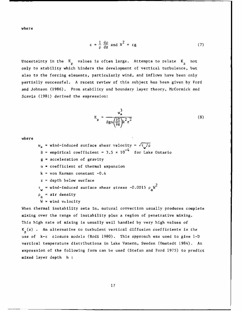
1 dp N2= -- andN = cg (7)p dz

Uncertainty in the K values is often large. Attempts to relate K notz z

only to stability which hinders the development of vertical turbulence, but

also to the forcing elements, particularly wind, and inflows have been only

partially successful. A recent review of this subject has been given by Ford

and Johnson (1986). From stability and boundary layer theory, McCormick and

Scavia (1981) derived the expression:

3u*

KzT 2 (8)Z ga - k z

where

u* = wind-induced surface shear velocity =

a = empirical coefficient = 3.5 x 10- for Lake Ontario

g = acceleration of gravity

= coefficient of thermal expansion

k = von Karman constant -0.4

z = depth below surface

Tw = wind-induced surface shear stress -0.0015 paW

Pa = air density

W = wind velocity

When thermal instability sets in, natural convection usually produces complete

mixing over the range of instability plus a region of penetrative mixing.

This high rate of mixing is usually well handled by very high values of

K (z) . An alternative to turbulent vertical diffusion coefficients is thez

use of k-E closure models (Rodi 1980). This approach was used to give I-D

vertical temperature distributions in Lake Vanern, Sweden (Omstedt 1984). An

expression of the following form can be used (Stefan and Ford 1975) to predict

mixed layer depth h

17

1 dh Apgh Z Constant (9)2dt 3

Pou*

where

Ap = density differential between mixed layer and next adjacent layerbelow

u* = shear velocity due to wind during time interval dt

When the stratification is strong, dissipation becomes important. Therefore

Equation 9 was extended by Bloss and Harleman (1979).

31. The transport and transformation of dissolved substances in a I-D

vertically stratified WQ model are described by an equation similar to

Equation 5.

V-C = Q z z + L A -Az + QiCi QoC ± S (10)at z az az z TZ, ii 0

Equations 5 and 10 are equivalent and are given by Orlob and Selna (1970) and

Huber, Harleman, and Ryan (1972), respectively. The sink/source term S

includes chemical and biological transformations and can take many different

forms. One of the simplest is a single first-order reaction. S = K1Cv ,

where K is a rate coefficient. For suspended materials, a settling term

- [(V sCA)/3z] x Az must be added to the right-hand side of the equation,

where V = settling velocity of the particles.s

32. There exist a large number of 1-D WQ models of the kind described.

A survey was given by Orlob (1983). The authors are acquainted with Orlob and

Selna's model (1970); Huber, Harleman, and Ryan's model (1972); Stefan,

Cardoni, and Fu's RESQUAL II (1982); Imberger and Patterson's DYRESM model

(Fischer 1981); the Hydrologic Engineering Center HEC-5 models (1986);

CE-QUAL-Rl (Environmental Laboratory (1986a); and Riley and Stefan's MINLAKE

model (1987). Other similar I-D reservoir models are the Tennessee Valley

Authority's (TVA's) WRMMS (TVA 1976) and RESTEMP (Brown and Shiao 1981)

models; and a USGS model (House 1981). All of these basically 1-D hydro-

dynamic models simulate temperature stratification, but CE-QUAL-RI and MINLAKE

also handle a large array of WQ parameters such as dissolved oxygen, algae,

nutrients, and conservative substances. CE-QUAL-RI is designed for reser-

voirs; MINLAKE is intended for lakes. A similar model FARMPOND for small

18

rural impoundments was developed by the US Department of Agriculture/

Agricultural Research Service.

33. The CE's vertically I-D model CE-QUAL-RI (Environmental Laboratory

1986a) simulates temperature plus as many as 34 other WQ parameters. Primary

physical processes included are surface heat transfer, shortwave and longwave

radiation and penetration, convective mixing, wind- and flow-induced mixing,

entrainment of ambient water by pumped-storage inflows, inflow density current

placement, selective withdrawal, and density stratification as impacted by

temperature and dissolved and suspended solids. Major chemical and biological

processes in CE-QUAL-RI include: the effects on DO of atmospheric exchange,

photosynthesis, respiration, organic matter decomposition, nitrification, and

chemical oxidation of reduced substances; uptake, excretion, and regeneration

of phosphorus and nitrogen and nitrification-denitrification under aerobic and

anaerobic conditions; carbon cycling and alkalinity-pH-CO 2 interactions;

trophic relationships for phytoplankton and macrophytes; transfers through

higher trophic levels (i.e. zooplankton and fish); accumulation and decomposi-

tion of detritus and organic sediment; coliform bacteria mortality; and

accumulation and reoxidation of manganese, iron, and sulfide when anaerobic

conditions prevail.

34. The US Army Engineer Waterways Experiment Station (WES) has

expended considerable effort during the past 20 years to develop a single gen-

eralized model for prediction of outflow water quality at dams, building on

the work of Brooks and Koh (1969) and many others. Smith et al. (1987) syn-

thesized the various point sink models into a single generalized, point sink

model. The WES's selective withdrawal models have been coded into a docu-

mented program referred to as SELECT (Davis et al. 1987). When used as a

stand-alone program, SELECT computes the in-pool vertical distribution of out-

flow and outflow concentrations of WQ constituents, given the in-pool vertical

distribution of water density and WQ constituent concentrations, the outlet

configuration and depth, and the discharge rate. In subroutine form, SELECT

is used in reservoir WQ models, e.g. CE-QUAL-RI (Environmental Laboratory

1986a), to compute the outflow distribution and release water quality.

Numerical hydrodynamic models for stratified flow, such as the WESSEL

(Thompson and Bernard 1985) and STREMR (Bernard, in preparation) codes, can be

used as experimental tools to study the withdrawal characteristics of unusual

outlet configurations.

19

Two-Dimensional Models of Reservoirs, Ponds, and Lakes

35. Two-dimensional (2-D) WQ models were developed for long, deep

reservoirs in which significant vertical WQ gradients are coupled with hori-

zontal ones. For example, Lake Powell and Lake Mead reservoirs on the

Colorado River require such an approach. A few 2-D models are available. One

is the Laterally Averaged Reservoir Model (LARM) model developed by Edinger

and Buchak (1983) and Buchak and Edinger (1984a, 1984b); another is the Com-

putation of Reservoir Stratification (COORS) model by Waldrop, Ungate, and

Harper (1980); Harper and Waldrop (1980a, 1980b); and TVA (1986). Both models

solve advection/diffusion equations in a vertical-longitudinal plane through a

reservoir. The models are width integrated. These models can predict the 2-D

temperature structure of deep reservoirs throughout the annual stratification

cycle and compute temporal and spatial hydrodynamics of reservoirs to provide

advective components for WQ models. A later version of LARM, referred to as

CE-QUAL-W2 (Environmental Laboratory 1986b), has been modified by the CE to

include 20 WQ constituents.

36. Temperatures and velocity gradients of deep storage reservoirs

occur primarily in the longitudinal (x) and vertical (z) directions. However,

lateral (y) contributions of shear stress, continuity, etc., are important,

but their effects can be included through an integration procedure in the

lateral direction. This procedure reduces by one the number of equations and

independent variables by eliminating the y-momentum equation and simplifying

the remaining equations. Additionally, most vertically stratified

hydrodynamic/transport models for reservoirs (and other surface waters) make

the hydrostatic assumption, which reduces the vertical equation to a simple

pressure gradient relation.

37. Empirical functions are defined to include the effects of turbulent

processes that orcur at a scale smaller than the resolution afforded by the

solution procedure (i.e., a finite difference grid). The technique chosen in

the COORS model is to assume that the effects of turbulence could be incorpo-

rated by using Prandtl's mixing length hypothesis where the mixing length is

defined by half the vertical spacing between grid planes.

38. Boundary conditions included in most 2-D models are inflows and

outflows (flow rate and temperature must be specified for inflows), bedshear,

no heat transfer through the bed, heat flux through the free surface, and

20

surface wind shear. These conditions are similar to those imposed in the I-D

models.

39. The numerical solution of the equations in the COORS model is

explicit and time marching, whereas the water surface solution of the

CE-QUAL-W2 model implicit, so that larger time-steps can be taken. Finite

differences are used to discretize the equations in both models.

40. CE-QUAL-W2 consists of directly coupled hydrodynamic and WQ trans-

port models. Hydrodynamic computations are influenced by variable water

density caused by temperature, salinity, and dissolved and suspended solids.

Developed for reservoirs and narrow, stratified estuaries, CE-QUAL-W2 can

handle a branched and/or looped system with flow and/or head boundary condi-

tions. With two dimensions depicted, point and nonpoint loadings can be

spatially distributed. Relative to other 2-D models, CE-QUAL-W2 is efficient

and cost-effective to use.

41. In addition to temperature, CE-QUAL-W2 simulates as many as

20 other WQ variables. The physical, chemical, biological processes of

CE-QUAL-W2 are very similar to those in CE-QUAL-RI with the following excep-

tions: it does not include transfer to higher trophic levels of zooplankton

and fish; it does not account for substances that are accumulat'ed in the sedi-

ments other than organic matter; it contains only one algal group rather than

three; it does not include macrophytes; and it does not include the sediment

release and oxidation of sulfur and manganese when anaerobic conditions pre-

vail, although it does allow specification (as a boundary condition) of flux

from the sediments of iron, ammonia nitrogen, and phosphate phosphorus during

anaerobic conditions.

42. A box model approach to 2-D reservoir modeling was used by Brown

(1985). The model, named BETTER for Box Exchange Transport Temperature and

Ecology of Reservoirs, has been applied to TVA reservoirs. In this model, the

reservoir is segmented into an array of volume elements or boxes. These boxes

are described with a volume, an upper interface or surface area, and a down-

stream conveyance area. The BETTER model uses a floating layer scheme, so

that the layer boundaries remain at specified depths relative to the surface

elevation. The layer spacing is arbitrary and can be changed by the user if

vertical gradients are not being adequately reproduced.

43. In the BETTER model, the flow patterns in the lake or reservoir are

modeled as longitudinal and vertical flow transfers between the array of

21

volume elements. Daily flow patterns can be calculated based on the inflow

and outflow. The flow patterns are influenced by the temperature patterns.

The inflow temperature governs where the inflow will enter the water column,

and subsequent flows will move through the reservoir along matched density

pathways. In addition to horizontal and vertical flows (transport), vertical

mixing (exchange) can be simulated. Mixing may be caused by wind surface

cooling or turbulent flows. Volumetric exchanges between adjacent layers or a

diffusive formulation can simulate mixing. A surface mixed layer can be cal-

culated for each day in response to surface cooling and wind mixing.

44. An introduction to box-type multidimensional model was given by

Chen and Smith (1979) and a review by Shanahan and Harleman (1984). A 2-D

box-type model for water quality has also been used for Lake Erie (Lam,

Schertzer, and Fraser 1983).

45. The most recent development in 2-D reservoir modeling include

(a) the replacement of eddy diffusion coefficients and mixing length theories

by other turbulence closures, e.g. k-c models, and (b) the solution of the

fundamental, fully convective primitive equations on powerful supercomputers.

Examples of this approach have been given by Ni et al. (1985), Thompson and

Bernard (1985), Farrell and Stefan (1986), and Sauvaget (1987). At this stage

of development, these models are pure hydrodynamic models. Water temperature

(or water density) is the only WQ parameter used.

46. Selection of a width-integrated x,z-coordinate system in a vertical

plane is appropriate fot 2-D models of long and deep reservoirs. Depth-

integrated models using x,y-coordinates are appropriate for shallow and wide

lakes. Bennett, Clites, and Schwab (1983) described a typical 2-D lake circu-

lation model. These models are typically driven by wind shear and include no

stratification effects on vertical turbulence since they are depth integrated.

This approach was used to model Lake Balaton in Hungary (van Straten and

Somlyody 1980). Other examples are given by Shanahan and Harleman (1984).

Three-Dimensional Models of Reservoirs, Ponds, and Lakes

47. Three-dimensional (3-D) WQ models have not been used extensively

because of the computational expense, as well as for other reasons. Lake and

reservoir 3-D flow simulations have been made by Simons (1973, 1975, 1976) and

Leendertse and Liu (1975) and verified in both small and large lakes. A

22

special version was produced by Kielmann and used for pollutant transport in

the Baltic Sea (Funkquist and Gidhapen 1984). The model uses seasonally and

depth-varied (six layers) eddy viscosities and eddy diffusivities. These

models do not overcome the uncertainty in the turbulence closing, but the pre-

dicted circulation is a reasonable synthesis of wind-induced and thermocline

circulation. The diffusive transport created by turbulence smaller than the

grid size in the horizontal (several kilometres) is modeled by a Monte Carlo

technique. This means that the calculated turbulent part of the parti-le

velocity is related to the eddy diffusivity in a physically correct way. Some

results obtained for the North American Great Lakes have been used in a 3-D WQ

model for Lake Ontario (Thomann et al. 1975; Thomann, Winfield, and Segna

1979). The WQ models are of the multiple-box type, i.e. multilayered in the

vertical and each layer subdivided into very large elements representative of

the coastal regions and the pelagic waters (Figure 5). Advective and disper-

sive flows between boxes are determined by flow budgets based on long-term

observed hydrology. Relying on the National Oceanic and Atmospheric Adminis-

tration Geophysical Fluid Dynamics Laboratory, researchers at Princeton and

Stevens Institute of Technology are compiling a massive 3-D time-dependent

model of the New York-New Jersey estuary. A similar effort is being conducted

by the WES for studying eutrophication problems in Chesapeake Bay.

23

LONGITUDINAL SEGMENT NO.. DELTA-X *1.0 KM LONGITUDINAL SEGMENT NO_* DELTA-X *1.0 KM

0.

7.0

LONGITUDINAL SEGMENT NO.. DELTA-X -1.0 KM 9.0 LONGITUDINAL SEGMENT NO., DELTA-X -1.0 KM2 6 10 14. 18 22 26 30 2 6 10 14 18 22 26 30

--.--- 120

1010 M< 1I2 6 *2 6 1 4 I 2 2 02

> I

0 0842 84?

11 NOV MBE 1980 25 NOVEMBE 1980K

242

4 7 1 15 19 24 5 33 37 41 45 5051

2 1 5 13 17 21 28 2 3)1 3 39 43 47

17-4 Meters 50-10 Meters

17150 Meters

Figure~~~~~~~~~0-5 5.LkM emnain(rmToaoetears175

25p

PART III: WATER QUALITY MODELS FOR FLOWING WATER (STREAMS AND RIVERS)

Approaches

48. Water quality models for streams and rivers range from relatively

simple analytical models to more sophisticated unsteady flow models. In

stream and river systems, the greatest WQ gradients generally occur or are

assumed to occur along the flow axis, and I-D (longitudinal) models that

employ cross-sectional averaging are usually appropriate. Although this

assumption may be valid for much of a modeled stream system, it can be vio-

lated for some localized regions, such as near discharges and downstream of

the confluence of two streams. Two-dimensional analytical solutions (Fischer

et al. 1980, Holley and Jirka 1986) resolve the spread and dilution of efflu-

ent plumes. These mixing models also address the question of whether a pol-

lutant has been sufficiently diluted to meet discharge standards. Selection

of an appropriate mixing model can be a tedious task if one is not familiar

with the various models and their assumptions. The USEPA, Athens, GA, is

incorporating these models and their protocols into an expert system to facil-

itate their use. This expert system will lead the user through the proper

model selection and use.

49. Herein a distinction is made between stream WQ models and stream

mixing models. Water quality models predict changes in WQ constituents due to

transport, loadings, and reactions. Stream mixing models typically predict

the initial mixing, spread, and dilution (as discussed previously), and some-

times downstream transport of a pollutant loading, but omit constituent

interactions and reactions. Stream mixing models treat the pollutant as con-

servative and are therefore not appropriate for far-field stream WQ studies.

For the latter, I-D models are used, and often instantaneous mixing of the

effluent across the stream is assumed. Although this assumption contradicts

reality in localized regions near discharges, it is a practical and meaningful

way of addressing most stream WQ issues. There exist a variety of approaches

for 1-D stream WQ models that range from steady-state analytical solutions to

dynamic numerical models.

26

Analytical and Numerical Steady-State Models ofStream and River Water Quality

50. Analytical solutions for I-D stream WQ models can be derived for

steady-state DO and BOD with simple first-order decay and sedimentation terms.

Gromiec, Loucks, and Orlob (1983) provided formulations and solutions for a

number of these models. Steady-state analytical solutions have the advantage

that they can be quickly applied and have minimal data requirements. Their

major disadvantage is that they require substantial simplification of stream

geometry and that they do not provide time-varying information that may be

required to fully address many questions.

51. Computerization of steady-state, analytical models allows easy sim-

ulation of more complex systems, such as stream networks. The USGS Streeter-

Phelps model (Bauer, Jennings, and Miller 1979) and the Corps of Engineers

STEADY model (Martin 1986) are examples of analytical models that allow a

steady-state solution for a stream network. STEADY models temperature, DO,

and BOD; the USGS Streeter-Phelps model computes DO and the components of

nitrogenous oxygen demand in addition to carbonaceous biochemical oxygen

demand (CBOD), orthophosphate phosphorus, total and fecal coliform bacteria,

and three conservative substances.

52. When assumptions that facilitate analytical solutions either become

inappropriate or do not allow for enough flexibility, it becomes necessary to

resort to numerical WQ models. Numerical WQ models for river and streams vary

widely in the amount of detail allowed, the number and type of WQ constit-

uents, and whether or not the model allows for time-varying conditions. The

following discussion provides an overview of two 1-D, numerical, stream WQ

models that are representative of other models of their type.

53. An example of an intermediate modeling approach between fully

dynamic and steady-state models is found in QUAL2E (Brown and Barnwell 1985),

a model developed through and maintained by the USEPA. QUAL2E is a numerical,

1-D (longitudinal) WQ model that assumes steady flows (steady-state hydraul-

ics) but allows simulation of either steady-state or dynamic WQ (diel varia-

tions). The model allows simulation of a total of 15 WQ constituents

including: DO, CBOD, temperature, algae as Chl a, organic nitrogen, ammonia

nitrogen, nitrite nitrogen, nitrate nitrogen, organic phosphorus, dissolved

(inorganic) phosphorus, coliforms, an arbitrary nonconservative constituent,

27

and three arbitrary conservative constituents. QUAL2E has been widely used

and is an accepted standard, particularly for waste-load allocation studies of

stream systems.

54. QUAL2E simulates a series of piece-wise nonuniform, steady-flow

segments referred to as reaches. Thus, the flows throughout the system are

constant with time and uniform within each reach, but the flow and hydraulic

characteristics can vary from reach to reach. The model is flexible in allow-

ing the simulation of point and nonpoint loadings, withdrawals, branching

tributaries, and in-stream hydraulic structures.

55. QUAL2E is easier to use than fully dynamic models (time-varying

flow and WQ) because of the steady-state hydraulic feature. Hydraulic condi-

tions are determined by any of three methods: (a) using stage-discharge

relationships for each reach; (b) solution of Manning's equation with pris-

matic chanrel geometry information given for each reach; and (c) entering

hydraulic information from another external source, such as a hydraulic step

calculation, e.g. HEC-2 (Hydrologic Engineering Center 1982) or stream gaging

information. Time-varying flow updates can be used with the model (Hamlin and

Nestler 1987) without excessive error if the changes in flow are small and

introduced gradually with respect to the system travel time.

Dynamic Models of Stream and River Water Quality

56. Fully dynamic models are required where transient events are of

importance and where significant flow variations occur over periods that are

much less than the travel time for the reach of interest. For example, if the

travel time for a particular flow is greater than its duration, then only a

portion of the reach would be exposed to that flow and its associated quality

at a given time. Using steady-state hydraulics, such as in QUAL2E, the flows

for all reaches would have to be incremented to the new flow condition instan-

taneously. In a fully dynamic model, the effects of time-varying flows and

quality along the reach are considered. Fully dynamic stream WQ models are

time-varying, hydraulic, or hydrologic-routing models coupled with time-

varying constituent transport and transformation models.

57. A number of fully dynamic, stream WQ models are in existence

(Jobson 1981, 1987; Bedford, Sykes, and Libicki 1983, Hydrologic Engineering

Center 1986.). A modified version of the Bedford model, referred to as

28

CE-QUAL-RIVi (Bedford, Sykes, and Libicki 1982), includes features specifi-

cally for regulated streams. CE-QUAL-RIVI has been applied by the Corps of

Engineers to a variety of regulated stream environments, including tailwaters

below peaking hydropower dams, stream re-regulation (Zimmerman and Dortch

1988), and run-of-the-river navigation pools.

58. The CE-QUAL-RIVI modeling package contains two codes, RIVIH for

hydraulic routing and RIVIQ for WQ routing. RIV1H, which is similar to

Fread's model (1978), solves the nonlinear St. Venant equations using the

four-point implicit finite difference method with a Newton-Raphson convergence

for nonlinearity. The model's formulation allows simulation of dynamically

coupled branched river systems with multiple hydraulic control structures,

such as weirs and low head dams. Boundary conditions may be provided in terms

of flows, stages, or rating curves.

59. RIVLQ is driven by output from RIVIH or any other flow-routing

model. RIVLQ uses an explicit finite difference method to solve the constitu-

ent mass balance equations. A two-point, fourth-order accurate scheme (Holly

and Preissman 1977) is used for the advection term. This means that the model

can accurately resolve the transport of sharp WQ gradients with little numeri-

cal diffusion. This feature can be important when simulating dynamic flow and

loading conditions or when tracking a spill. The model is similar to QUAL2E

in that it models temperature, DO, CBOD, and nutrient kinetics. Reaeration

takes into account stream reaeration, wind-driven reaeration, and reaeration

through control structures.

Inputs and Mixing Zones

60. Inputs are usually classified as point source (PS) or nonpoint

source (NPS). In the vicinity of a pollutant source, one usually finds higher

concentration gradients than in the receiving water body. The purpose of a

mixing zone analysis or model usually is to determine the flow and concentra-

tion gradients in the vicinity of PS discharges (Lam, Murthy, and Simpson

1984).

61. Mixing zone analysis for pollution PS can have two different objec-

tives: (a) to show sufficient dilution of an effluent near its discharge

point so that a specified concentration (effluent WQ standard) is not exceeded

beyond specified distances from the outlet or (b) to determine the distance

29

required to mix an effluent nearly uniformly (e.g. 0.9 C < C < 1.1 C) with a

river cross section or a layer in a stratified reservoir.

62. A mixing zone model describes the location of the isopleths as a

function of river and outlet channel geometry, river flow, and effluent flow

conditions. The development of the model must take into consideration the

hydrodynamics of the situation. For example, a side channel discharge inter-

acts with a river flow in several ways before the two become fully mixed.

Among the flow and mixing processes generally to be considered are (Stefan

1982, Stefan et al. 1984, Muellenhoff et al. 1985): (a) jet effects due to

the momentum of the discharge; (b) lateral displacement of river flow by the

effluent input; (c) downstream advection by the river flow: (d) transverse

turbulent mixing including secondary flow in the river; (e) buoyant spreading

caused by the density difference between effluent water and river water--

density depends on water temperature and total solids content; (f) vertical

turbulent mixing by the river due to bed shear; and (g) mixing by navigation,

structures, and similar man-made effects.

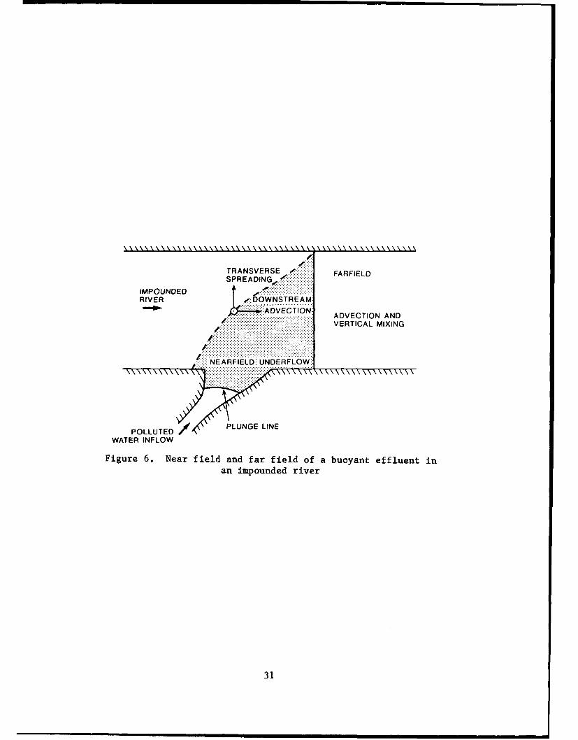
63. To facilitate the analysis, it can sometimes be considered that

some of the processes occur in sequence, e.g. jet mixing before buoyancy

effects. Effluent models are usually subdivided into a near field and a far

field (Figure 6). In the near fieid, the mixing and dilution are influenced

hydrodynamically by effluent conditions. In the far field, the mixing is

passive and imposed by the receiving water conditions. Far field models are

usually 2-D and use the advection/diffusion equation in either a horizontal or

vertical plane (Krishnappan and Lau 1982, 1985). If a density differential

exists between the effluent and the receiving water, a density-stratified flow

may develop, especially if the receiving water is an impounded river or a

lake.

64. When effluent discharges are from pipes, the near field mixing

analysis may require the application of jet flow models and, in the case of

complex geometries, recourse to physical models. There exist specialized

numerical models for the analysis of PS releases, e.g. DISPER or TADPOL

(Almquist et al. 1977) for passive mixing in the far field, and various jet

and plume mixing models in uniform or stratified ambients, e.g USEPA's PDS

model (Shirazi and Davis 1974) and Ditmars' (1969) submerged jet models. For

a discussion of this highly specialized topic, the reader is referred to

Fischer et al. (1979) and Hoiley and Jirka (1986).

30

TRANSVERSE : FARFIELDSPREADING

IMPOUNDEDRIVER ...-:DOWNSTREAM:

1 .. ADVECTION:ADVECTION ANDVERTICAL MIXING

............ ........................

NEARFIELD: UNDERELOW

POLL.UTED/P

WATER INFLOW

Figure 6. Near field and far field of a buoyant effluent in

an impounded river

31

=.. • =m=,-=,==i= = = m~.........n....... I I .

PART IV: SEDIMENT TRANSPORT AND SEDIMENT/WATER QUALITY INTERACTIONS

Concepts

65. Sediment is typically associated with agricultural runoff. Sedi-

ment not only affects water transparency, but can carry chemicals such as

nutrients and toxic substances into receiving waters. Therefore, an important

aspect of WQ modeling is the capability to simulate sediment transport and

sediment/water interactions.

66. Aquatic sediment transport has two main forms: bed load and sus-

pended load. Although both forms of transport can be important in streams,

suspended transport is of primary interest in standing waters. Even when

there is no sediment transport by the flow, sediments deposited on the bed of

a stream, reservoir, or lake and not in motion can have a strong influence on

WQ in the overlying water. Through adsorption, biofilm, and other chemical/

biochemical transformations, stream or lake sediments can become sinks or

sources of materials such as oxygen, toxic materials, or nutrients.

67. For WQ, suspended sediment and moving or stationary bed sediments

are of primary interest particularly for the finer fractions of materials

including silts, clays, organic detritus, and live plankton materials. Parti-

cles are characterized by size, shape, density, surface area, and surface

physical and chemical properties including electric charges. Lal (1977) gives

a review of particle regimes, composition, behavior, and interaction with

water density.

Processes

Fall velocities, settling, deposition

68. For WQ modeling, the fall velocity of particles and their resis-

tance to resuspension under shear stress, once they are deposited, are most

significant. Fall velocities are functions of size, shape (drag coefficient),

and density and can be reasonably well predicted for larger mineral particles

(Dietrich 1982; Gibbs, Matthews, and Link 1971). For micron-size particles

and particularly for organic particles, the large diversity in sizes, shapes,

and density (Lal 1977, Ives 1973) often requires indirect determinations of

fall velocities from settling traps or mass balances. Settling velocities are

32

used to calculate the movement of sorbed chemical downward through the water

column. The deposition velocity can be estimated as the product of the set-

tling velocity and the probability of deposition upon contact with the bed,

which may range from 0 for fast, turbulent streams to 1 for stagnant pools.

Resuspension, scouring, erosion

69. Difficult also is the determination of rates of resuspension under

bed shear action. For granular noncohesive materials, the relationship is

"explosive" in nature. Very low or no resuspension occurs until a threshold

shear stress is reached. Then resuspension rates increase proportional to

some power of the excess shear stress. Powers of one have been found in estu-

arine studies, but powers of four and five have been found for granular river

material according to a review by Akiyama and Fukushima (Wang, Shen, and Ding

1986). Rate of resuspension can be balanced by rate of deposition. At that

point vertical concentration profiles above the bed show a balance of downward

fluxes of sediment by settling and upward fluxes by turbulence as summarized

by Vanoni (1975). According to Rouse (Vanoni 1975), the dimensionless param-

eter Vs(Ku*) -1 determines for flow over flat bottoms the degree for which

vertical sediment distribution will be uniform. It will be uniform within

±10 percent when V s(KU) -1 is less than -0.02. V = particle fall veloc-

ity, K = 0.4, and u, = bed shear velocity = VT,7/ with T = bed shear andb b

p = water density.

70. Rates of resuspension of noncohesive materials have been specified

in numerous alternative forms by Ariathurai and Krone (1976); Ariathurai

(1982); and Mehta (1986); Wang, Shen, and Ding (1986). Akiyama and Fukushima

(Wang, Shen, and Ding 1986) specified a dimensionless resuspension rate

parameter E as:

E =3 x 101 2 10 (I- )for 5 < Z < 13.4 (11)

E = 0.3 for Z > 13.4s

where

u,

Z =7--Rs

1/2 DR = (g'D) --

p

33

= g(p /p - 1) = reduced acceleration of gravity of submergedparticles

D = particle diameter

= kinematic viscosity

The resuspension (or scour or erosion) rate depends not only upon the shear

stress on the benthic surface and the sediment size but also on the state of

consolidation of the surficial benthic depositc. Site-specific calibration is

necessary to refine initial estimates of scour.

Cohesion

71. Cohesion of particles in the deposited bed increases the resistance

to resuspension and is a function of the degrees of consolidation. The inves-

tigation of this behavior by Krone, Ariathurai, Partheniades, and others have

been reviewed by Mehta (1986). Besides bed shear stresses due to gravity or

wind driven flows, perturbations by navigation or organisms (bioturbation) can

greatly increase rates of resuspension of cohesive sediments. Effect on

resuspension by wind was conceptualized by Rodney and Stefan (1987).

Coagulation and flocculation

72. Coagulation is a physical/chemical process by which particles form

flocs. The flocs have higher settling velocities, and this fact affects water

quality in a very significant way. This effect is used in wastewater

treatment. Its significance in freshwater bodies has been studied by O'Melia

(1980), among others.

Sorption

73. Suspended sediment, besides being a very important WQ parameter in

its own right, can also have a very strong relationship with chemical species

dissolved in the water through adsorption/desorption, e.g. of nutrients or

synthetic organics (often toxic materials). This is an area of very active

research (Golterman, Sly, and Thomas 1983; Stumm and Morgan 1981; Karickhoff

1984) and will be addressed in a later section in more detail.

Bottom boundary layer

74. The interaction between particles and water chemistry becomes par-

ticularly complex near the bed because of (a) strong velocity gradients in the

vertical associated with shear forces; (b) activities of organisms such as

biofilms, invertebrates, crustaceans, and fish; and (c) pore water movement

which leaches into and out of the outlying waters. Microcosm models of these

systems are necessary to provide the input or withdrawal rates of dissolved

34

substances. Examples are sedimentary oxygen demand (Chen, Brannon, and Gunni-

son 1984; Gantzer et al. 1988), phosphorous release, and PCB resuspension.

Turbidity currents

75. Sediment suspended in water can increase the density of the water/

sediment mixture significantly enough so that density currents can form in

"standing" waters when such mixtures are released near the shore or water sur-

face. Particles can be deposited from such currents or eroded from the bed,

and as a result, buoyancy flux is not conserved. Turbidity currents can be

generated by wave action in shallow areas of lakes or reservoirs, by longshore

currents, or simply by inflows; they provide a mechanism by which pollutants

attached to sediment can be rapidly transported over long distances from shal-

low littoral waters to profundal waters. The mechanics of the erosive phase

of such currents and I-D models for their analysis exist (Akiyama and Stefan

1985) and can be incorporated in reservoir WQ models. The depositional phase

of these currents is still under investigation.

Model Formulations

76. In stratified lakes and reservoirs of moderate size, advection in

the horizontal direction is rapid, relative to vertical mixing, and hence only

vertical gradients in SS concentration are simulated. One-dimensionality is

often an acceptable assumption for smaller water bodies (of length <20 km). A

relationship among SS concentration profiles, vertical turbulence, rate of

deposition, and resuspension is

a(V AC) A 1A C A--A a(z + V C R zsVC-+z A z- -(R- (12)

where C = suspended sediment concentration and V = fall velocity of suspendeds

sediment in quiescent water. The first term in this equation represents the

change in sediment content with time, the second term is the rate of transfer

by settling from one layer to another, the third term is the rate of deposi-

tion on the sloping lake bed, the fourth term is the vertical turbulent mixing

rate, and the last term is the resuspension. Vertical advection can be added

to this equation.

35

77. There exist sediment transport models for specific purposes, e.g.

modeling of alluvial channels (Dawdy and Vanoni 1986), reservoir sedimentation

(Hydrologic Engineering Center 1977), estuarine water movement and sediment

transport (King 1982), or simple lake turbidity (Stefan, Cardoni, and Fu

1982). Most of these models can be found referenced in recent proceedings of

conferences dealing with river sedimentation (Wang, Shen, and Ding 1986),

coastal engineering (Mehta 1986), reservoirs (Stefan 1981, Thomas and McAnally

1985), and lakes (Lerman 1978). Many of these models are concerned mainly

with the quantity of sediment transport, locations of erosional or deposi-

tional areas, channel modification, etc. Models dealing with suspended parti-

cle transport including inorganic and organic (detritus and phytoplankton)

particles and their interaction with water quality have been developed mostly

for applications in eutrophication control discussed in Part V.

Examples of One-, Two-, and Three-Dimensional Sediment Transport Models

One-Dimensional Models

78. HEC-6 (Hydrologic Engineering Center 1977) computes both flow and

transport. It is designed to analyze scour and deposition in rivers and

reservoirs. HEC-6 and similar models are used when the flow is unidirectional

and constrained to follow well-defined channels. It calculates transport of

sands, silts, and clays and can handle bed-load and suspended-load transport.

A 1-D turbidity model is the RESQUAL II model (Stefan, Cardoni, and Fu 1982).

It computes the unsteady, vertical distribution of suspended sediment and uses

it to determine light penetration for primary productivity. The attenuation

coefficient n is calculated as the cumulative effect of the water, the sus-

pended inorganic sediment (SS) concentration, and the Chl a concentration.

n = a + bSS + c Chl a (13)

Two-dimensional models

79. Two-dimensional models include those that are integrated over depth

(horizontal models) and those that are integrated over width (vertical

models).

80. Horizontal 2-D modeling of sediment transport is performed by

STUDH, which is part of the TABS-2 modeling system (Thomas and McAnally 1985).

36

STUDh is a finite element model designed for situations where the flow and

transport can be satisfactorily described by depth-integrated equations.

STUDH computes the bed-load or suspended-load transport of silts or clays. It

obtains flows either by specification or from the TABS-2 flow model, RMA-2V.

It calculates transport due either to currents alone or to currents plus sbort

period waves (nonbreaking). The program allows for wetting and drying of

cells and consolidation of fine sediments with overburden and time.

81. Laterally averaged models are applicable in studies of relatively

deep narrow water bodies. Work on models of this type has been more limited

than on the depth-averaged models. However, work performed during the past

few years has produced a useful model, LAEMSED, produced (Johnson, Trawle, and

Kee, in preparation) by adding sediment transport capability to the basic

hydrodynamic/transport model LARM2 (Edinger and Buchak 1983), on which

CE-QUAL-W2 is also based. A layered bed model allows for the exchange of

material between the water column and the bed, but only SS transport is simu-

lated. This model has been used to investigate the effect of navigation

channel deepening on salinity intrusion and sediment transport (Johnson,

Trawle, and Kee, in preparation).

Three-dimensional models

82. Two sets of three-dimensional models are in use by the WES for SS

transport. They are the Resource Management Associates (RMA) series and

CELC3D. Both models have a free surface, are time dependent, and allow for

stratification and complex geometry.

83. The RMA series. The RMA series of programs model flow and

transport in three dimensions using a finite element method. Program RMA-8

(King 1982) computes water levels and currents for constant density flows.

Program RMA-10 (King 1982) computes water levels, currents, and salinity/

temperature transport for flows with density gradients. SEDIMENT 8

(Ariathurai 1982) computes transport for sands, silts, or clays and contains

information from Ariathurai and Krone (1976). The models permit parts of the

computational mesh to be two-dimensional while employing the full three dimen-

sions in other areas, thus ensuring economical operation.

84. CELC3D. The 3-D finite difference model of Coastal, Estuarine, and

Lake Currents, CELC3D (Sheng 1983), simulates hydrodynamics and transport for

temperature, salinity, and sediment. Special features include (a' a "mode-

splitting" procedure which allows efficient computation of the vertical flow

37

structures (internal mode); (b) an efficient alternating direction implicit

(ADI) scheme for the computation of the vertically integrated variables

(external mode); (c) an implicit scheme for the vertical diffusion terms;

(d) a vertically and horizontally stretched coordinate system; and (e) a tur-

bulence parameterization. CELC3D provides for the resuspension, transport,

and deposition of sediments where sediment particle dynamics are modeled by a

consideration of particle groups and coagulation processes. Detailed dynamics

within a turbulent boundary layer, under pure wave or wave-current interac-

tion, is evaluated by means of a turbulence submodel.

85. Other 3-D models of estuaries and coastal seas were developed by

Leendertse (1970, Leendertse and Liu (1975), and Onishi and Trent (1982).

38

PART V: MODELS ADDRESSING ORGANIC WASTES AND NUTRIENTS

Concepts

86. Water quality problems created by organic waste and nutrients

include depletion of DO and stimulation of nuisance aquatic growth. In addi-

tion, high levels of nitrate or ammonia can be harmful to aquatic life.

87. Organic waste is generated by farm operations and may be carried to

ponds and streams by runoff. Nutrients such as nitrogen and phosphorus are

applied to fields as fertilizer and can reach surface waters by runoff and

leaching. Nitrogen is more soluble and is easily mobilized by runoff or

leachate water. Phosphorus is more strongly bound to soil, but may be carried

by erosion. The organic matter and nutrients contained in agricultural runoff

can play an important role in the trophic state and WQ of receiving waters.

This section is a brief overview of the processes for modeling these constit-

uents (referred to as conventional pollutants) and their interactions. For

more detailed information, the reader should refer to other sources (Chapra

and Reckhow 1983, Orlob 1983, Bowie et al. 1985, Thomann and Mueller 1987).

The focus of models of conventional pollutants can be DO and BOD as a general

measure of the health of the system, or it can be primary productivity when

eutrophication is the major concern. These models usually include tempera-

ture, major nutrients, other chemical characteristics, detritus, bacteria, and

primary producers. Water quality models for surface waters may include higher

trophic levels (i.e. zooplankton and fish) because of their effect on other

more important variables, such as phytoplankton, BOD, and DO. Zooplankton and

fish also provIde a means of controlling lower trophic levels, which can

impact nutrients and DO (biomanipulation). Because the source of agricultural

organic waste and nutrients is driven by the hydrologic cycle, the most

appropriate modeling approaches are dynamic. For steadier leaching or irriga-

tion situations, however, steady-state or quasidynamic models may be adequate.

Fate Processes

88. Upon entry to the surface water body, settling of particulate

organic waste and nutrients generally occurs. High flow events may lead to

scouring of previously deposited material. Organic matter is oxidized,

39

drawing upon the DO supply, which is replenished by reaeration. Organic

nitrogen is mineralized to ammonia, which reaches ionic equilibrium with

ammonium. Nitrification further draws upon the DO supply converting ammonia

to nitrite and then nitrate. Nitrate may be converted back to ammonia or to

nitrogen gas through denitrification in low DO regions of the water or sedi-

ment. Ammonia and nitrate may be taken up by phytoplankton and aquatic plants

and incorporated into the food chain, eventually returning to the water as

organic nitrogen.

89. Organic phosphorus is mineralized to orthophosphate, which comes to

sorptive equilibrium with suspended or benthic sediment. Particulate sorbed

phosphate settles; dissolved phosphate is rapidly taken up by phytoplankton

and aquatic plants and incorporated into the food chain, eventually returning

to the water as organic phosphorus.

90. Organic material deposited to benthic sediment is oxidized in the

upper aerobic layer and reduced in the lower anaerobic layers. Upward fluxes

of ammonia and reduced organic species are produced, the latter contributing

to sediment oxygen demand. Particulate phosphorus may be resolubilized and

may reenter the water. In some aquatic environments, net sedimentation buries

a good fraction of the nutrients and organic matter deposited to the bed.

91. Although many of these interacting fate pathways are well known and

included in most recent conventional WQ models, accurate simulations remain

difficult. Extensive site-specific data collection is required to character-

ize both the sources and the rates under a range of expected conditions. Many

of the rates are biologically mediated, with descriptive constants and param-

eters that vary both with environmental conditions and predominant species.

The major pathways and cycles will be briefly discussed from the model devel-

oper's perspective.

Phytoplankton kinetics

92. Phytoplankton kinetics assume a central role in eutrophication

affecting the nitrogen and phosphorous cycles, the DO balance, and food chain

response. The reaction term for phytoplankton is expressed as the difference

between the growth rate and the death and settling rates in a volume element.

The growth rate of a phytoplankton is a complicated function of the species

present and their differing reactions to solar radiation, temperature, and the

balance between nutrient availability and phytoplankton requirements. Avail-

able information does not allow specification of growth kinetics for

40

individual species in a natural environment. Hence, models either simulate

the phytoplankton community as a whole or as classes such as greens, diatoms,

blue-greens, and dinoflagellates.

93. The growth rate G is usually formulated as the product of the

maximum 200 C growth rate (under optimum light and nutrient conditions) with a

temperature adjustment factor, a light adjustment factor, and a nutrient limi-

tation factor.

G = G XTXLXN (14)

94. Temperature is an important WQ variable because of its effect on

transformation and reaction rates and aquatic life. Temperatures are calcu-

lated as described in the section on 1-D temperature stratified reservoir

models. The temperature adjustment factor is usually given as

XT = 0T-200 (15)

where 0 is a species-specific coefficient.

95. Light attenuation functions XL generally follow the analysis by

Steele (1962, 1965), accounting for the effects of supersaturating light

intensities and light attenuation through the water column, and lead to

= exp o -exp Kexp -) (16)2"v1 ex nd- ep] I K e

sI

where-1

= light extinction coefficient (including self shading), m

d = depth, m

I = incident light intensity just below the surface, ly/day0

I = saturating light intensity of phytoplankton, ly/days

This expression is either integrated over the day or multiplied by the frac-

tion daylight. Generally I is used as a calibration parameter. Smiths

(1980) developed a framework for calculating I based upon the maximum

growth rate, thequantum yield of chlorophyll, the extinction coefficient per

unit of chlorophyll, and the ratio of carbon to chlorophyll in the

41

phytoplankton. This framework allows for adaptation by changing the carbon to

chlorophyll ratio. Recent developments in phytoplankton kinetics models use

photosynthetically active radiation (PAR) in pE m2 day- instead of total

energy I (ta day -). They also apply Haldane kinetics in place of Steele's

equation (Megard, Tonkyn, and Senft 1984).

96. The nutrient limitation factor is based on the assumption that phy-

toplankton follow Monod kinetics with respect to the important nutrients.

Generally, the minimum function for inorganic nitrogen and phosphorus is used:

XN = Mn (G IN ' P (17)

where

CIN = inorganic nitrogen, ug/t

KMN = Michaelis half-saturation constant for nitrogen, Ug/t

C = inorganic phosphorus, pg/k

KMP= Michaelis half-saturation constant for phosphorus, vg/k

Occasionally, XN is expressed as the product of the nitrogen and phosphorous

terms.

97. Phytoplankton "death" rates are conventionally expressed as the sum

of the endogenous respiration rate, the death rate, and the grazing rate. The

first two are generally modeled as a first-order temperature corrected rates.

Grazing may be expressed as first order, or second order if the herbivorous

zooplankton population is specified or simulated. To capture the phytoplank-

ton population dynamics properly, zooplankton may have to be simulated. If

average phytoplankton levels are adequate, then the first-order approach is

acceptable.

98. Phytoplankton kinetics affect the nitrogen, phosphorus, and carbon

cycles primarily through uptake and secondarily through death. Proper speci-

fication of average stoichiometry is necessary to accurately model these

interactions. The ratios of phytoplankton carbon to phytoplankton nitrogen,

phosphorus, and chl a vary among species and in time. Few applied-modeling

frameworks account for the dynamics of stoichiometry. The user is forced to

specify average values or those characteristic of stressed systems.

42

The phosphorous cycle

99. Organic phosphorus in the water is present in various particulate

and dissolved forms that mineralize and settle at different rates. Some

models lump all organic phosphorus into a single-state variable, while others

divide organic phosphorus into two-, three-, or four-state variables that dif-

fer in settling and mineralization rates. Mineralization or bacterial decom-

position is generally modeled as first-order temperature-corrected reaction,

although second-order and saturating rates based upon phytoplankton biomass

have been employed.

100. Dissolved inorganic phosphorus sorbs to suspended-particulate

matter in the water column, coming to an equilibrium expressed either with a

partition coefficient or as a calibrated fraction dissolved:

f = 1 (18)DIP 1 +K PI5S

wherefDIP = fraction inorganic phosphorus dissolved,

KplP = partition coefficient, Q./kg

SS = suspended sediment concentration, kg/9

Subsequent settling of the solids and sorbed phosphorus can provide a signifi-

cant loss mechanism of phosphorus from the water column to the benthos.

Process-based functions that accurately calculate the phosphorous partition

coefficient would improve prediction of this important variable significantly.

101. Dissolved inorganic phosphorus is taken up by phytoplankton at the

stoichiometrically modified growth rate. While there is evidence for "luxury

storage" of inorganic phosphorus in phytoplankton, most models assume only one

internal pool of phosphorus as biomass. Grazing causes transfer of phyto-

plankton phosphorus up the food chain. Upon respiration and death, biomass

phosphorus is recycled to the various forms of organic and inorganic phos-

phorus at user-specified ratios.

The nitrogen cycle

102. Organic nitrogen in the water is present as various particulate

and dissolved forms that mineralize and settle at different rates. As for

organic phosphorus, some models lump all organic nitrogen into a single-state

variable, while others divide organic nitrogen into two-, three-, or

43

four-state variables. Mineralization to ammonia can be represented as first

order or can include second-order or saturating dependence on phytoplankton

biomass.

103. Ammonia nitrogen in the presence of nitrifying bacteria and oxygen

is converted to nitrite, then nitrate nitrogen. The process of nitrification

in natural water is complex, depending upon DO, pH, total inorganic carbon,

alkalinity, Nitrosomonas and Nitrobacter bacteria, and flow conditions. Most

models represent the reaction with a first-order, temperature-corrected rate

constant. Some allow spatial variations calibrated by the user, or empirical

DO limitations terms. Obviously, a process-based predictive function for this

rate would be quite valuable.

104. Denitrification is the reduction of nitrate to ammonia and nitro-

gen gas. Primarily a benthic reaction, it is included in some models as a

loss rate of nitrate. It is modeled as a first-order reaction, sometimes

multiplied by a modified Michaelis-Menten term to suppress the reaction in the

presence of a small amount of oxygen.

105. Both ammonia and nitrate are taken up by phytoplankton at the

stoichiometrically modified growth rate. Some models include a preference

function that calculates mostly ammonia uptake when its concentration is high

enough. Grazing causes transfer of phytoplankton nitrogen up the food chain.

Upon respiration and death, biomass nitrogen is recycled to the various forms

of organic nitrogen and ammonia at user-specified ratios.

The carbon-dissolved oxygen balance

106. Organic carbon is present in water in various particulate and dis-

solved forms that oxidize and settle at different rates. Some models lump all

organic carbon into a single-state variable expressed in units of oxygen--

carbonaceous biochemical oxygen demand, CBOD. Other models represent various

fractions of organic carbon, with their separate oxidation and settling rates.

Oxidation is generally modeled as first-order temperature-corrected rate.

Some allow spatial variations calibrated by the user.

107. Traditional models of organic waste do not compute inorganic car-

bon and the associated variables of pH and alkalinity. This carbonate system

could be important for simulating the effects of acidic wastes on unionized

ammonia concentrations or potential carbon dioxide limitation in low-

alkalinity, high-nutrient waters. Models that include the carbonate system

calculate total inorganic carbon as the sum of bicarbonate, carbonate, and

44

carbon dioxide. These species are in equilibrium controlled by the equi-

librium constants of the dissociation reactions and the pH of the water. Car-

bon dioxide (and thus total inorganic carbon) is produced by resp4 ration,

consumed by algal growth, and replenished by atmospheric exchange. Carbonate

alkalinity is the sum of bicarbonate concentration, two times the carbonate

concentration, an4 the hydroxide concentration miius -he hydrogen ion concen-

tration. Addition of acids and nitrification lowers the pH and reduces alka-

linity. Nitrate uptake by phytoplankton produces hydroxide and increases

alkalinity.

108. Dissolved oxygen is depleted by oxidation of organic carbon,

nitrification, and respiration. Benthic reactions depleting oxygen are usu-

ally modeled as a spatially variable flux of sediment oxygen demand. Respira-

tion effects may be combined for simplicity or separated into components such

as respiration by bacteria, plankton, macrophytes, fish, etc. The respiration

of decomposers that utilize organic matter is referred to as decomposition.

Oxygen is used during some chemical transformations, such as nitrification and

the oxidation of reduced substances (e.g. sulfide, methane, reduced iron, and

reduced manganese).

109. Biochemical oxygen demand (BOD) is a measure of the oxidizable

matter due to biochemical processes. The problem with BOD is that it combines

the effects of several oxygen-consuming processes into one variable; this

approach may be too simple for modeling some systems. The more realistic

approach is to separate oxygen demands into various components, such as bio-

degradable organic (carbonaceous) demands, nitrogeneous demands, and oxidation

of other substances (e.g. reduced metals, sulfide, etc.). Biodegradable

organic demands may be due to dissolved and particulate matter in the water

column and bottom sediments. Some models separate water column organic matter

into particulate and organic matter (POM) and dissolved organic matter (DOM).

Because some forms of organic matter decay at faster rates than others,

organic matter may be further divided into those that decay at a fast rate

(labile) and those that decay at a slower rate (refractory). As labile

organic matter decomposes, a portion is transferred to the refractory state.

A similar approach can be used for organic sediments. Sources of organic

matter include external waste loads and excretion and mortality of living

substances.

45

110. Dissolved oxygen is replenished by phytoplankton growth (photo-

synthesis) and by reaeration. Many reaeration formulas exist for streams and

rivers. Those based solely on velocity and depth include O'Connor-Dobbins

(for slower, deeper rivers), Churchill (for moderately deep, faster streams),

and Ownes et al. (for shallow streams) (see Thomann and Mueller 1987). The

Tsivoglou method calculates reaeration in rive'rs and streams from the slope

and travel time. Relationships that include the effects of bed roughness,

secondary flow, and wind are under development. Numerous relationships exist

for wind-induced reaerstion in lakes and reservoirs. There remains a need for

critical review and assimilation of all the formulas. Reaeration at hydraulic

structures can be very significant.

Benthic-water interactions

111. The decomposition of organic material in benthic sediment can sig-

nificantly affect the concentrations of oxygen and nutrients in the overlying

waters. Aereal fluxes from the sediment due to diagenetic reactions can be

substantial nutrient sources oL oxygen sinks. The occurrence of anoxia may

dramatically increase nutrient fluxes.

112. Most traditional models described these benthic fluxes as spa-

tially variable source and sink terms. Some recent modelg have included

benthic compartments where state variables are simulated. Particulate nitro-

gen, phosphorus, and carbon are added to the bed by settling and are lost by

scour or sedimentation (burial). Dissolved species of nitrogen, phosphorus,

carbon, and oxygen exchange with overlying water by pore water diffusion.

Benthic oxidation rates are generally assumed first-order, with low rate con-

stants producing ammonia and consuming organic carbon and oxygen equivalents

(functionally, reduced organic species that are oxidized at the water inter-

face). Recently, efforts have been made to simulate the diagenetic reactions

and resulting fluxes more realistically (DiToro 1986). These efforts hold

great promise for more accurate and predictive modeling of organic and nutri-

ent wastes.

Simulation Models

113. Numerous simulation models of organic waste e.d nutrients have

been developed and applied to various water bodies. Of these, only a few have

been maintained for general application. To be useful for general

46

agricultural nutrient and organic waste simulations, a model should allow for

unsteady transport and loading, phytoplankton kinetics, nitrogen and phos-

phorous cycles, and carbon-dissolved oxygen balances. Furthermore, written

documentation and a user's manual must be available with the software.

114. Five modeling frameworks meet these criteria: WASP4-(EUTR04),

CE-QUAL-Ri, CE-QUAL-W', CE-QUAL-RIVI, and HSPF. QUAL2E may be useful for

steady-loading situations. Such models as DEM, EXPLORE, RECEIVII, WRECEV,

MINLAKE, and AUTO-QD meet these criteria but are not actively maintained and

supported by a central, public distribution center. Different versions of

these and others may be maintained privately by consultants and local Govern-

ment agencies and may be useful for those water bodies where setup and cali-

bration have previously been accomplished.

115. Stream Quality Model QUAL2E (Brown and Barnwell 1985) is a steady-

state model for conventional pollutants in I-D streams and well-mixed lakes.

The conventional pollutants include conservative substances, temperature,

bacteria, BOD, DO, nitrogen, phosphorus, and algae. QUAL2E is widely used for

waste-load allocations and discharge permit determinations in the United

States and other countries. WASP is designed to permit easy substitution of

user-written routines into the program structure. Problems that have been

studied using WASP include BOD, DO dynamic, nutrients and eutrophication, bac-

terial contamination, and toxic chemical movement.

116. Eutrophication WASP (EUTRO4) (Ambrose et al. 1988) combines a

kinetic structure adapted from the Potomac Eutrophication Model with the WASP

transport structure. EUTR04 predicts DO, CBOD, phytoplankton, carbon, and

chl a, ammonia, nitrate, organic nitrogen, and orthophosphate in the bed and

overlying waters.

117. WASP4 is linked to DYNHYD4 (Ambrose et al. 1988), a simple link-

node hydrodynamic model capable of handling variable tidal cycles, wind, and

unsteady inflows. It produces an output file that can be linked with WASP4 to

supply the flows and volumes to the WQ model.

118. Hydrological Simulation Program FORTRAN (HSPF) (Johanson et al.

1984) is a comprehensive package for simulation of watershed hydrology and

WQ for both conventional and toxic organic pollutants. HSPF incorporates the

watershed-scale Agricultural Runoff Model (ARM) and NPS models into a basin-

scale analysis framework that includes pollutant transport and transformation

in stream channels.

47

119. The model uses information such as the time history of rainfall,

temperature, and solar radiation; land-surface characteristics such as land-

use patterns and soil properties; and land-management practices to simulate

the processes that occur in a watershed. The result of this simulation is a

time history of the quantity and quality of runoff from an urban or agricul-

tural wntershcd. Flow rate, sediment load, and nutrient and pesticide concen-

trations are predicted. The program takes these results, along with

information about the stream network and PS discharges, and simulates instream

processes to produce a time history of water quantity and quality at any point

in a watershed--the inflow to a lake, for example. HSPF includes an internal

data base management system to process the large amounts of simulation input

and output. The models CE-QUAL-RI, CE-QUAL-W2, and CE-QUAL-RIVI were dis-

cussed in previous sections.

48

PART VI: SYNTHETIC ORGANIC CHEMICALS

Fate Processes

Ionization

120. Ionization is the dissociation of a chemical into multiple-charged

species. Consider a weak acid AH3 or base BH3

AH _AH + H , K (19)3 2 al

BH B BH + OH-, 1i (20)

These reactions are rapid. At equilibrium, the distribution of chemicals

between the unionized and the ionized species is controlled by the pH of the

water and the ionization constants.

121. Stronger acids and bases may undergo further ionization, con-

trolled by ionization constants Ka 2 , Ka 3 , Kb2 , and Kb3 * Ionization

can be important because of the different toxicological and chemical

properties of the unionized and ionized species.

Sorption

122. Sorption is the bonding of dissolved chemicals onto solid phases

Si , such as benthic and suspended sediment, biological material, and sometime

dissolved or colloidal organic material.

Si + C0C - Si (21)

These reactions are usually fast relative to other environmental processes,

and equilibrium may be assumed. For environmentally relevant concentrations

(less than 10- 5M or one-half water solubility), equilibrium sorption is linear

with dissolved chemical concentration (Karickhoff 1984) or:

Ci = Kpi x Cd (22)

where

C i = chemical concentration in phase i, mg/kg

Kpi = the sorption partition coefficient for phase i, Q./kg of phase i

Cd = dissolved chemical concentration, mg/9.

49

At equilibrium, then, the distribution among the phases is controlled by the

partition coefficients K . The total mass of chemical in each phase is

controlled by Kpi and the amount of solid phase present.

123. Values for the partition coefficients can be obtained from labora-

tory experiments. For organic chemicals, lab studies have shown that the par-

tition coefficient is related to the hydrophobicity of the chemical and the

organic matter content of the sediment. Normalization of the partition coef-

ficient by the organic-carbon content of the sediment has been shown to yield

a coefficient, KOC , that is relatively independent of other sediment charac-

teristics or geographic origin. Correlation of KOC with the water solubil-

ity of the chemical or the octonal/water partition coefficient of the chemical

has yielded successful predictive tools for incorporating the hydrophobicity

of the chemical in an ..stimate of its partitioning. These correlations do

poorly for chemicals with very low or very high hydrophobicity, however,

because of deviations from hydrophobic adsorption. Chemicals containing polar

functional groups and low octanol/water partition coefficients tend to exhibit

hydrophilic contributions to adsorption, whereas large nonpolar molecules with

high octanol/water partition coefficients generally require long periods to

reach equilibrium resulting in low estimates of KOC when sorption is mea-

sured over short time frames. The latter effect is particularly significant

because it suggests that the assumption of instantaneous equilibrium used by

the toxic chemical models may not be valid for those chemicals for which

adsorption is the most important process.

124. In addition to the assumption of instantaneous equilibrium,

implicit in the use of Equation 22 is the assumption of reversibility. Lab-

oratory data for very hydrophobic chemicals suggest, however, that a

hysteresis exists, with desorption being a much slower process than adsorp-

tion. Karickhoff (1984) suggests that this effect may be the result of

intraparticle kinetics in which the chemical is slowly incorporated into com-

ponents of the sorbant. This phenomenon is not well understood. A quantita-

tive modeling framework to characterize it was proposed by Di Toro (1985).

125. Sorption can be important in controlling both the environmental

fate and the toxicity of chemicals. Sorption may cause the chemical to accu-

mulate in bed sediments or bioconcentrate in fish. Sorption may retard such

reactions as volatilization and base hydrolysis or may enhance other reactions

including photolysis and acid-catalyzed hydrolysis.

50

Settling, deposition, and scour

126. Suspended particles carrying sorbed chemicals can settle through

the water column and deposit on the underlying bed. Benthic particles carry-

ing sorbed chemicals can scuur and become suspended in the water column. Mass

fluxes for settling, deposition, and resuspension are controlled by the set-

tling, deposition, and scour velocities, and the concentrations of suspended

and benthic sediment.

Loss kinetics

127. Chemical concentrations and resulting observed toxic effects often

decline downstream due to physical and chemical reactions. For constant envi-

ronmental conditions, the overall chemical loss rate is often approximated as

a first-order reaction:

mk = _KT X C X V (23)

where-I

KT observed loss coefficient, in days

C = total chemical concentration, g/m3

3V = volume of water plus sediment, m

The observed loss coefficient KT represents a single set of environmental

conditions only. Changes in temperature, velocity, depth, sunlight, wind,

sediment concentration, or pH can affect the total loss rate in unknown ways.

128. A method to complement field survey data is the chemical process

approach. This approach combines laboratory-measured chemlcal constants with

field-measured environmental properties to estimate site-specific rate coeffi-

cients, K i(x,t) , for several loss processes "i";

K.(x,t) = Ki x E i(xt) (24)

where Ki is a laboratory-measured second-order rate constant and E i(x,t)

is the intensity of the relevant environment parameter. If more than one loss

process is active for a chemical in an environment, the overall loss coeffi-

cient can be estimated by summing the individual rate constants. Combining

the chemical process approach with the field survey approach should increase

the reliability of modeling estimates, allowing extrapolation to a much wider

range of environmental conditions.

51

129. The loss processes considered in most chemical fate models include

volatilization, hydrolysis, photolysis, and bacterial degradation. Chemical

oxidation and reduction are sometimes included as well.

130. Volatilization is the flux of a chemical across the air-water

interface. Its rate is proportional to the gradient between the dissolved

concentration in the overlying atmosphere. For most chemicals, the partial

pressure in the atmosphere is negligible and the equation reduces to a

first-order form with the removal rate coefficient, K , expressed:v

K = -k x fd x d-1 (25)v v d

where

k = conductivity of the chemical, m/sv

fd = fraction of the chemical concentration that is dissolved

d = average water depth, m

131. The conductivity is influenced by both chemical properties

(molecular weight, Henry's Law constant) and environmental conditions at the

air-water interface (turbulence-controlled by wind speed, current velocity,

and water depth). Toxic chemical models either require the user to input a

value for k or internally compute a value using the two-film theory firstv

proposed by Lewis and Whitma. (1924). This theory assumes that the rate of

transfer is controlled by diffusion through laminar layers in the air and

water at the interface in which the concentration gradients driving transfer

are localized.

132. The liquid and gas transfer coefficients are dependent on

turbulence at the interface, on temperature, and on properties of the chemical

such as diffusivity. Empirical correlations have been developed relating

transfer coefficients either directly to physical parameters such as wind

velocity and the density and viscosity of the water (Southworth et al. 1979a;

MacKay and Yeun 1983), plus the molecular weight and diffusivity of the

chemical or to the field-measured transfer coefficients of oxygen and water

vapor (Liss and Slater 1974). O'Connor (1983) has presented a theoretical

development of the liquid transfer coefficient applicable to a wide range of

hydrodynamic conditions, but application requires estimates of several

coefficients and wind data that are not easily obtained.

52

133. Hydrolysis is a reaction in which cleavage of a molecular bond of

the chemical and the formation of a new bond with either the hydrogen or the

hydroxyl component of a water molecule occurs. Hydrolytic reactions are

usually catalyzed by acid and/or base, and the overriding factor affecting

hydrolysis rates at a given temperature is generally hydrogen or hydroxide

concentration (Wolfe 1980). The overall hydrolysis rate constant in most

toxic chemical models is calculated by:

= £(k, x [ H+) + kHNi + kHBi [O]) (26)

where

kH i = acid hydrolysis rate constant for phase i, L/mole-s

[H ] = hydrogen ion concentration, moles/L-1

kH i = neutral hydrolysis rate constant for phase i, skB = alkaline hydrolysis rate constant for phase i, L/mole-s

[OH ] = hydroxide ion concentration, moles/L

The models do not compute hydrogen or hydroxide ion concentrations. Instead

these are input to the models assuming that their concentrations are unaf-

fected by the hydrolysis reaction because of the low concentration of the

toxic chemical present and reacting.

134. Photodegradation (photolysis) is the transformation or degradation

of a compound that results directly from the adsorption of light energy. It

is a function of the quantity and wavelength distribution of incident light,

the light adsorption characteristics of the compound, and the efficiency at

which absorbed light produces a chemical reaction. Photolysis is classified

into two types that are defined by the mechanism of energy absorption. Direct

photolysis is the result of direct absorption of photons by the toxic chemical

molecule. Indirect or sensitized photolysis is the result of energy transfer

to the toxic chemical from some other molecule that has absorbed the

radiation.

135. A quantitative framework that permits the prediction of direct

photolysis from the incident light and the characteristics of the chemical

(Zepp and Cline 1978) has been incorporated in several of the toxic chemical

modeling frameworks. Use of this framework in natural water systems is com-

plicated by the lack of a satisfactory model of ultraviolet-light penetration

that incorporates the effects of both dissolved organics and particulate

53

material in the water. A comprehensive framework for photolysis also must

include sensitized photolysis. Unfortunately, the spectrum of compounds,

particularly dissolved organics, involved in photochemical reactions is not

known (Miller 1983). In addition, valid frameworks to predict free radical

reactions have not been developed, and the importance of these reactions

remain undetermined (Zepp 1980).

136. A less rigorous method for predicting a photolysis rate coeffi-

cient K involved extrapolations of observed rates from one environmentalp

condition to another:

K p= G x (L) x E Pi x fi (27)

where-1

KPG = observed rate coefficient in s for a reference light intensity

[L] = fraction of the reference light intensity averaged throughwater column

OPi = relative yield for the chemical in phase i

f, = fraction of the total chemical concentration in phase i

The reference light fraction [L] accounts for depth, light extinction, cloud

cover, latitude changes, and surface light variability.

137. Biodegradation encompasses the broad and complex process of

enzymatic attack by organisms on organic chemicals. Bacteria, and to a lesser

extent fungi, are the mediators of biological degradation in surface water

systems. Dehalogenation, dealkalytion, hydrolysis, oxidation, reduction, ring

cleavage, and condensation reactions are all known to occur either metaboli-

cally or via cometabolism. Cometabolism refers to degradation of chemicals by

microorganisms that are not capable of utilizing the chemical as a substrate

for growth. Biodegradation is generally assumed to follow Michaelis-Menten

enzyme kinetics. Values for the half-saturation constant K and the maximumm

rate of degradation are not easily measured. Toxic chemical models generally

assume that the chemical concentration is much less than the half-saturation

constant and simplify the Michaelis-Menten equation to:

-1KB max x K × B = -k x B (28)

where KB is the second-order rate coefficient in millilitres per cells per

day. The bacterial activity, B in cells per millilitres, is fundamentally the

54

concentration of the enzyme reacting with the toxic chemical. Enzyme concen-

tration cannot be measured in the field; however, the environmental and eco-

logical effects on its activity are difficult to estimate (Lewis et al. 1984).

138. The growth kinetics of the bacterial population degrading a toxic

chemical are not well understood. The presence of competing substrates and of

other bacteria, the toxicity of the chemical to the degrading bacteria, and

the possibilities of adaptation to the chemical or cometabolism make quantifi-

cation of changes in the population difficult. As a resiult, toxic chemical

models assume a constant biological activity rather than modeling the bacteria

directly. Often, measured first-order biodegradation rate constants from

other aquatic systems are used directly.

Simulation Models

139. Numerous simulation models have been developed for toxic chemicals

in surface water systems. Of these, only a handful have been developed for

general application. To be useful for general agricultural chemical simula-

tions, a model must include benthic and water column compartments, unsteady

transport and loading, partitioning and transformation reactions. Further-

more, written documentation and a user's manual must be available along with

the software.

140. Seven modeling frameworks described here meet these criteria:

EXAMS (Burns et al. 1982, Burns and Cline 1985), a quasi-dynamic model for

organics; WASP (DiToro et a,. 1983; Ambrose et al. 1983, 1986, 1988; Connolly

and Winfield 1984) and HSPF (Johanson et al. 1984), dynamic compartment models

for organics and metals; SERATRA (Onishi and Wise 1982), FETRA and TODAM, l-

and 2-D dynamic models for organics and metals; and UTM-TOX (Browman 1983), a

dynamic multimedia model for organics and metals. These frameworks differ

mainly in the degree of specificity incorporated in the transport, transfer,

and reaction processes, the allowable spatial and temporal resolution of the

problem, and the manner in which sediment is defined.

141. Exposure Analysis Modeling System (EXAMS-II) is both a steady-

state and a quasi-dynamic model designed for rapid evaluation of the behavior

of synthetic organic chemicals in aquatic ecosystems, including lakes, rivers,

and estuaries. EXAMS-II is an interactive program that allows the user to

specify and store the properties of chemicals and ecosystems, modify the

55

characteristics of either via simple Englishlike commands, and conduct rapid,

efficient evaluations of the probable fate of chemicals. EXAMS-II simulates a

toxic chemical and its transformation products using second-order kinetics for

all significant organic chemical reactions. EXAMS-II does not simulate the

solids with which the chemical interacts. The concentration of solids must be

user-specified for each compartment. The model accounts for sorbed chemical

transport based on solids concentrations and specified transport fields.

Benthic exchange includes pore water advection, pore water diffusion, and

solids mixing. The latter describes a net steady-state exchange associated

with solids that is proportional to pore water diffusion. EXAMS is supported

by USEPA's Center for Exposure Assessment Modeling, Athens, GA.

142. Water Quality Analysis Simulation Program (WASP4) (Ambrose 1988)

is a generalized modeling framework for contaminant fate in surface waters

including lakes, rivers, and estuaries. Based on the flexible compartment

modeling approach, WASP4 can be applied to 1-, 2-, or 3-D given transport

between segments. WASP4 can read output files from the link-node hydrodynamic

model DYNHYD4, which predicts unsteady flow rates in unstratified rivers and

estuaries given variable tides, wind, and inflow. A variety of WQ problems

can be addressed with the selection of appropriate kinetic subroutines. Two

general toxic chemical modeling frameworks have been constructed from WASP-

TOXIWASP (Ambrose et al. 1983) and WASTOX (Connolly and Winfield 1984,

Connolly and Thomann 1984). These separate frameworks are combined in WASP4.

The WASP models are supported by USEPA's Center for Exposure Assessment Model-

ing, Athens, GA.

143. The TOXI4, subset of WASP4, simulates up to three interacting

toxic chemicals and up to three sediment size fractions in the bed and over-

lying waters. First- or second-order kinetics can be used for all significant

organic chemical reactions. Benthic exchange includes pore water advection,

pore water diffusion, and deposition/scour. Net sedimentation and burial

rates can be specified or calculated. An empirically based food chain model

is linked to TOXI4 for calculating chemical concentrations in biota and fish

resulting from predicted aquatic concentrations.

144. Hydrological Simulation Program FORTRAN (HSPF) is a comprehensive

package for simulation of watershed hydrology and WQ for both conventional and

toxic organic pollutants. The HSPF simulates three sediment types (sand,

silt, and clay) in addition to specific organic chemicals and transformation

56

products of those chemicals. The reaction and transfer processes included are

hydrolysis, oxidation, photolysis, biodegradation, volatilization, and sorp-

tion. Sorption is modeled as a first-order kinetic process in which the user

must specify a desorption rate and equilibrium partition coefficient for each

of the three solids types. Resuspension and settling of silts and clays

(cohesive solids) are defined in terms of shear stress at the sediment-water

interface. For sands, the capacity of the system to transport sand at a par-

ticular flow is calculated, and resuspension or settling is defined by the

difference between the sand in suspension and the calculated capacity. Cali-

bration of the model requires data for each of the three solids types. Ben-

thic exchange is modeled as sorption/desorption and deposition/scour with

surficial benthic sediments. Underlying sediment and pore water are not

modeled. The HSPF is supported by USEPA's Center for Exposure Assessment

Modeling, Athens, GA.

145. The Sediment Radionuclide Transport Model (SERATRA) framework

(Onishi and Wise 1982) is a time-variable model for simulating radionuclides

or organic chemicals in river systcms. It solves the 2-D (vertical and longi-

tudinal) advection-dispersion equation using finite element techniques for one

chemical and three types of solids (sand, silt, and clay). Scour and deposi-

tion of solids are defined in identical fashion to that in HSPF. The transfer

and reaction processes included are hydrolysis, photolysis, oxidation, bio-

degradation, volatilization, and sorption. Volatilization is computed from a

user-specified oxygen transfer coefficient, limiting consideration of volatile

organics to those that are liquid-film controlled. Sorption is modeled as a

first-order kinetic process for each of the three solids types. Benthic

exchange is modeled as sorption/desorption and deposition/scour with surficial

benthic sediments. Underlying sediment and pore water are not modeled. A

similar I-D (longitudinal) version for rivers (TODAM) and a 2-D (longitudinal

and lateral) version for estuaries (FETRA) are also available from Batelle

Pacific Northwest Laboratories, Richland, WA.

146. The Unified Transport Model for Toxicants (UTM-TOX) (Browman

et al. 1983) is an upgrade of the Unified Transport Model (UTM) originally

developed to model heavy metal ions. It is a time-variable framework that

includes atmospheric, terrestrial, and aquatic components. The aquatic

component is designed to simulate streams and rivers. The transfer and

reaction processes include sorption, volatilization, hydrolysis,

57

biodegradation, and first-order photolysis. Sorption is described by an equi-

librium partition coefficient. Sorbed phases are assumed unreactive (1982

version). UTM-TOX is available from Oak Ridge National Laboratories, Oak

Ridge, TN.

58

PART VII: METALS

147. Metals are found naturally in the Earth's crust. As a result of

irrigation in some regions, metals may be solubilized and transported to sur-

face waters. Steady or quasi-dynamic modeling approaches should be adequate

if irrigation practices do not change.

Fate Processes

148. Upon entry to the surface water body, metal speciation may change

because of complexation, precipitation, sorption, and redox reactions. Metals

concentrations are further diluted by additional streamflow and mixing. Phys-

ical loss can be caused by settling and sedimentation, whereas a physical gain

may be caused by resuspension.

Metal complexation, precipitation

149. Heavy metals can form complexes with organic and inorganic liquids

and precipitate or dissolve:

M+ + L _ML 1 Kri (28)

M+ + L 2 ML2 , K 1 (29)

where

M = metal ionL and L2 = liquids (such as carbonate, sulfide, or humate)

ML 1 = soluble complex

K = equilibrium coefficient for reaction i

ML2 = insoluble complex

Ksp i = solubility product for reaction iReaction times range from essentially instantaneous to thousands of years. At

equilibrium, the distribution of metals among the possible complexes is con-

trolled by the amount of metal and liquids present and the reaction coeffi-

cients and solubility products. In natural waters, sorption also affects the

distribution by reducing the amount of metal available for complexation and

precipitation.

59

150. Complexation reactions can affect transport by either increasing

or decreasing the soluble fraction. Sometimes one chemical species is known

to be much more toxic than another for a given heavy metal. This is

especially important because some states and USEPA have been moving towards

"site-specific water quality standards," in which chemical speciation will be

considered on a site-by-site basis. For example, a site that is known to have

a great deal of naturally occurring dissolved organics may not require as

stringent a WQ standard because the dissolved organic material may complex the

heavy metal and render it nontoxic to biota.

Sorption

151. Heavy metals frequently absorb or "bind" to solid surfaces. The

mechanism of sorption or attachment is via: (a) physical absorption to solid

surfaces, (b) chemical sorption or binding by liquids at the solid water

interface, or (c) ion exchange with an ion at the solid water interface. In

addition, if the heavy metal is complexed in solution by an organic liquid, it

could sorb into the organic solid phase much like an organic pollutant. The

mathematical formulation for describing the partitioning of the heavy metal

between the solid phase and the aqueous phase is the same as for organic

chemicals except the K is usually called the "distribution coefficient"

for heavy metals (although it may be referred to as the partition coefficient

or the binding constant in some cases). In most measurements and simulation

models, all soluble complexes are lumped with the free ion to give the

dissolved metal concentration. Precipitated metal is lumped with all sorbed

species to give total particulate metal concentration. A spatially variable

lumped-distribution coefficient K% describes the two phases. There is no

general consistency in reported K D values for particular methods in the

natural environment, so site-specific values should be used when possible.

Redox reactions

152. Metals can change oxidation states through various oxidation and

reduction reactions:

M+ + + e K ri (30)

where

M = oxidized metal

e = an electron

60

M+ = reduced metal

Kri = equilibrium coefficient for reaction i

Under some conditions, the kinetics of oxidation or reduction may be important

to simulate.

Simulation Models

153. Two kinds of simulation models have been developed for metals in

surface water systems. One addresses aquatic transport and fate, while the

other addresses metals chemistry. The former are those general toxic chemical

models that include benthic and water column compartments, partitioning, and

particulate settling, resuspension, and sedimentation. These include MICHRIV,

a steady-state model for organics and metals; TOXIWASP, WASTOX, WASP3, WASP4,

and HSPF, dynamic compartment models for organics and metals; SERATRA, FETRA,

and TODAM, I- and 2-D models for organics and metals; and UTM-TOX, a dynamic

multimedia model for organics and metals. All of these have been discussed in

an earlier section.

154. The second kind of simulation model addresses metals chemistry.

Those developed for general application include organic and inorganic com-

plexation, sorption, precipitation and dissolution, and redox reactions.

These models are single compartment equilibrium models that calculate specia-

tion for specified environmental conditions based on a set of thermodynamic

constants. Environmental conditions, such as metal concentrations, liquid

concentrations, pH, pE, and temperature, must be specified by the user.

Thermodynamic constants are usually included in a data base with the model.

Examples of these models include MINTEQ (Felmy 1984) and MINTEQAI (Brown and

Shiao 1981); REDEQL and MINEQL; WATEQ (versions 1-4); and GEOCHEM.

155. Proper application of these models requires some specialized

expertise because kinetic limitations at particular sites may prevent the

thermodynamically possible reactions. Nevertheless, thoughtful application

may reasonably describe the predominant metals species at a site and thus give

useful insight into potential migration patterns and biological effects. For

agricultural leaching problems, these models must be run in conjunction with

one of the transport and transformation models described above.

156. MINTEQAL (Felmy et al. 1984, Brown et al. 1987) is a geochenical

model that is capable of calculating equilibrium aqueous speciation,

61

absorption, gas phase partitioning, solid phase saturation states, and

precipitation-dissolution of 11 metals (arsenic, cadmium, chromium, copper,

lead, mercury, nickel, selenium, silver, thallium, and zinc). MINTEQAl con-

tains an extensive thermodynamic data set and six different algorithms for

calculating absorption. MINTEQAI is supported by USEPA's Center for Exposure

Assessment Modeling in Athens, GA.

62

PART VIII: CHALLENGES AND RECOMMENDATIONS

157. Several challenges in the state of the art of WQ modeling are

apparent.

158. The composition of WQ models introduces and combines uncertainties

from several sources. A recent review by Beck (1987) examines (a) model

structure, (b) model parameters, (c) propagation of prediction errors, and

(d) experimental design to reduce critical uncertainties. In practical appli-

cations of WQ models, uncertainty in input data is often a major limitation.

In Beck's assessment, there is ample evidence that "larger," more "comprehen-

sive" models are easily capable of generating highly uncertain prediction of

future behavior. Figure 7 gives the frame of reference for the analysis of

uncertainty (Beck 1987). Aspects of model uncertainty are also addressed in

stochastic modeling (see Reckhow and Chapra 1983). Model sensitivity to

parameter variability and confidence levels of model outputs from probabilis-

tic distributions of inputs are sometimes generated. Progress in this area

will raise the reliability of models and help to identify "optimum sophistica-

tion in water quality modeling."

159. Current WQ concerns are with numerous toxic substances such as

heavy metals, e.g. mercury, lead, cadmium, and chlorinated organics (e.g. DDT,

PCB, Dieldrin, etc.). The pathways and ultimate fates of these substances

through ecosystems are often not fully understood, and thus, limit the

formulation of useful and reliable forecasting models at this time (Dolan and

Bierman 1982, Thomann and DiToro 1983). There is a need to improve under-

standing and descriptions for processes affecting contaminant transport and

fate, such as partitioning of contaminants to solids and bacterial decomposi-

tion. Additionally, work should focus on the transport of surface water con-

taminants to ground water. The verification of contaminant models has been

greatly limited by the expense of collecting appropriate data. Therefore,

confidence in these models will remain limited until proper verifications are

performed. As a tool to assess research needs, the models are, however, very

useful at this stage. Among the uncertainties are adsorption/desorption pro-

cesses, interactions of organics and sediments, and surface chemistry. The

formulation of adsorption isotherms frequently (Sweeney et al. 1982) pose

problems in model formulation. The problem applies to suspended sediments as

well as deposited (bottom) sediments.

63

zz0J

2 sa1.- 0 0u Lo Z D 4

0 CL < L UJ 0

< (r 00

w S 'S)0

z

04I

W UU

o0 CA

0- 'rI.4-4

cru~ o W

zo-w 0)

000

cr L) Cu C

kA 0 OcUrf -J

-J 0 -J Z 0>0 - CzW-

ZL 0- 0 0 4-4'-

A c- 0-) 0

~~-o 0Z4~rw~ - - -- - L I

i0 IA 0 4

04 wL

0 0 00 0~, z>0.k: M4- -4-2 W LJ

2J <0. 1

0 0

0. (r - 0 - L-

0 w cc

160. Models which quantify the role of pH in aquatic ecosystems have

been formulated (Schnoor et al. 1987; Lang 1987; Weater, Bishop, and Beck

1986) and are being refined with the intent to assist in the selection of

appropriate acid rain abatement strategies. While basic chemical relation-

ships to pH are known, the biological response can often not be quantified

yet.

161. The greatest need in the area of conventional (DO/nutrient) WQ

modeling is the development of reliable models that predict sediment diagene-

sis and fluxes from and to the bottom sediments. Water quality models will

not be truly predictive until the bottom sediments are interactively coupled

with the water column to provide time-varying SOD and nutrient fluxes that are

predictable from previous conditions. Although some work bhs been started in

this area (Hatcher 1986), there is still much study necessary. Proper sedi-

ment modeling will require an accounting of labile and refractory forms of

particulate and dissolved organic matter in both the water column and bottom

sediments.

162. Capabilities for "number crunching" by supercomputers continue to

rise dramatically. This appears to permit recourse to replace some empirical

relationships with more fundamental ones, e.g. in flow simulation or in chemi-

cal partitioning. It is likely that in the long term most of the benefits

will come from the ability to simulate long time frames in multidimensions

with the hydrodynamic and WQ model run on the same temporal and spatial

scales. The biological parameters will probably continue to require numerous

empirical relationships.

163. Spin-offs of artificial intelligence technology have resulted in

computerization of knowledge-based and expert systems. Development of these

systems for WQ models will improve user/computer interfaces and greatly reduce

th. difficulty of selecting and applying these models. Other related aspects

are the development of preprocessors and postprocessors, graphics, and other

decision support.

164. Although complexity of some WQ models makes their application for

daily decision making impractical, managers should understand what are avail-

able and now they can be used. The USEPA through its WQ modeling program and

other agencies and universities can provide modeling packages and assistance.

Some models are compact enough to be used on personal computers (PC's) and

micros. User-friendly programs developed for PC's permit decision-makers to

6-,

manipulate data bases and to screen management options. This can be useful

during managerial planning and policy discussions (Chapra and Canale 1987,

Canale and Auer 1987).

165. Remote sensing offers intriguing possibilities for synoptic inves-

tigation of large areas, e.g. of reservoirs. It appears that multispectral

scanner information can be correlated with some WQ parameters collected onsite

(ground truth). If these correlations can be strengthened in further

research, remotely sensed spatial distributions of surface WQ can be compared

with model simulations. This can be useful for model verification and also

for updating of initial conditions for model simulations. The combination of

remote sensing with WQ models may offer a reasonably inexpensive means to

follow WQ evolutions in real time, e.g. for reservoir management.

Table I

Some Typical WQ Models

All Water Pond, Lake,Parameters Bodies Reservoir River Estuary

Agriculturalpollutants

Sediment or WASP4 CE-QUAL-RI HSPF CE-QUAL-W2total suspended CE-QUAL-W2 SERATRA FETRAsolids RESQUAL II TODAM SED-III

Organic waste WASP4- CE-QUAL-RI QUAL2E CE-QUAL-W2and nutrients (EUTR04) CE-QUAL-W2 CE-QUAL-RIVI

MINLAKE HSPF

Synthetic EXAM-II HSPF FETRAorganics WASP4- SERATRA

(TOXI4) TODAMUTM-TOX

Metals WASP4- MICHRIV FETRAtransport (TOXI4) HSPF

SERATRATODAMUTM-TOX

Metals MINTEQAI

speciation MINEQLWATEQ3GEOCHEM

66

REFERENCES

Akiyama, J., and Stefan, H. G. 1984. Plunging Flow into a Reservoir:Theory," Journal of Hydraulic Engineering, American Society of Civil Engi-neers, Vol 110, No. HY4.

. 1985. "Turbidity Current with Erosion and Deposition," Journal

of Hydraulic Engineering, American Society of Civil Engineers, Vol 1i1,No. HY12.

1987. "Gravity Currents in Lakes, Reservoirs and Coastal

Regions: Two-Layer Stratified Flow Analysis," Project Report No. 253,St. Anthony Falls Hydraulic Laboratory, University of Minnesota, MN.

Almquist, C. W., Harper, W. L., Ungate, C. D., and Frank, M. G. 1977. "AModel of Dispersion of a Passive Species in a Reservoir with Application toRadionucleides Discharged from the Browns Ferry Nuclear Plant," ReportNo. 63-61, Tennessee Valley Authority, Water Systems Development Branch.

Ambrose, R. B., Jr., et al. 1983. "User's Manual for the Chemical Transportand Fate Model TOXIWASP Version I," EPA-600/3-83-005, US Environmental Protec-tion Agency, Athens, GA.

. 1986. "WASP3, A Hydrodynamic and Water Quality Model-Model

Theory, User's Manual, and Programmer's Guide," EPA-600/3-86-034, US Environ-mental Protection Agency, Athens, GA.

. 1988. "WASP4, A Hydrodynamic and Water Quality Model-ModelTheory, User's Manual, and Programmer's Guide," EPA-600-3-86-058, US Environ-mental Protection Agency, Athens, GA.

Annandale, G. W. 1987. "Reservoir Sedimentation," Developments in WaterScience, p 29.

Ariathurai, C. R. 1982. "Two- and Three-Dimensional Models for SedimentTransport," RMA 9180, Resources Management Associates, Lafayette, CA.

Ariathurai, C. R., and Krone, R. B. 1976. "Finite Element Model for CohesiveSediment Transport, Journal of Hydraulic Division, American Society of CivilEngineers, Vol 102, No. HY3, pp 323-338.

Bauer, D. P., Jennings, M. E., and Miller, J. E. 1979. "One-DimensionalSteady-State Stream Water Quality Model," US Geological Survey Water ResourcesInvestigation 79-45, Bay St. Louis, MS.

Beck, M. B. 1987. "Water Quality Modeling: A Review of Analysis of Uncer-tainty," Water Resources Research, Vol 23, No. 8, pp 1393-1442.

Bedford, K. W., Sykes, R. M., and Libicki, C. "A Dynamic, One-Dimensional,Riverine Water Quality Model," Contract Report in preparation, prepared underContract No. DACW39-82-M-3548 by Ohio State University for the US ArmyEngineer Waterways Experiment Station, Vicksburg, MS.

. 1983. "Dynamic Advective Water Quality Model for Rivers,"

Journal of Environmental Engineering Division, American Society of Civil Engi-neers, Vol 109, No. 3, pp 535-554.

Bennett, J. R., Clites, A. H., and Schwab, D. J. 1983. "A Two-DimensionalLake Circulation Modeling System: Programs to Compute Particle Trajectories

67

and the Motion of Dissolved Substances," National Oceanic Atmospheric Adminis-tration Technical Memorandum ERL GLERL-46, Ann Arbor, MI.

Bernard, R. S. "Explicit Numerical Algorithm for Modeling IncompressibleApproach Flow," Technical Report in preparation, US Army Engineer WaterwaysExperiment Station, Vicksburg, MS.

Bloss, S., and Harleman, D. R. F. 1979. "Effect of Wind-Mixing on the Therm-ocline Formation in Lakes and Reservoirs," Technical Report No. 249, R. M.Parsons Laboratory, Massachusetts Institute of Technology, Cambridge, MA.

Bowie, G. L., et al. 1985. "Rates, Constants, and Kinetics Formulations inSurface Water Quality Modeling," 2d ed., EPA/600/3-85/040, US EnvironmentalProtection Agency, Athens, GA.

Brooks, N. H., and Koh, R. C. Y. 1969. "Selective Withdrawal from Density-Stratified Reservoirs," Journal of Hydraulics Division, American Society ofCivil Engineers, Vol 95, No. HY4, pp 1369-1400.

Browman, M. G., et al. 1983. "Physio-Chemical Processes in the Environment:Background Information for the ORNL Unified Transport Model for Toxicants(UTM-TOX)," ORNL-5854, Oak Ridge National Laboratory, Oak Ridge, TN.

Brown, D. S., et al. 1987. "MINTEQAI, an Equilibrium Metal Speciation Model:User's Manual," EPA/600/3-87/012, US Environmental Protection Agency, Athens,GA.

Brown, L. C., and Barnwell, T. 0. 1985. "Computer Program Documentation forthe Enhanced Stream Water Quality Model QUAL2E," Report EPA/600-3-85/065,US Environmental Protection Agency, Athens, GA.

Brown, R. T. 1985. "BETTER, A Two-Dimensional Reservoir Water Quality Model:Model User's Guide," Center for the Management, Utilization, and Protection ofWater Resources, Tennessee Technological University, Cookeville, TN.

Brown, R. T., and Shiao, M. C. 1981. "Reservoir Temperature Modeling: CaseStudy of Normandy Reservoir," Report WR28-1-86-101, Tennessee Valley Author-ity, Water Systems Development Branch.

Buchak, E. M., and Edinger, J. E. 1984a. "Generalized, Longitudinal-VerticalHydrodynamics and Transport: Development, Programming and Applications," Doc-ument No. 84-18-R, US Army Corps of Engineers, Vicksburg, MS.

_ 1984b. "Simulation of a Density Underflow into Wellington Reser-

voir Using Longitudinal-Vertical Numerical Hydrodynamics," DocumentNo. 84-18-R, US Army Corps of Engineers, Vicksburg, MS.

Burns, L. A., and Cline, D. M. 1985. "Exposure Analysis Modeling Systems,Reference Manual for EXAMS II," EPA-600/3-85-038, US Environmental ProtectionAgency, Athens, GA.

Burns, L A., et al. 1982. "Exposure Analysis Modeling System (EXAMS): UsersManual and System Documentation," EPA-600/3-82-023, US Environmental Protec-tion Agency, Athens, GA.

Canale, R. P., and Auer, M. T. 1987. "Personal Computers and EnvironmentalEngineering. Part II - Applications," Environmental Science and Technology,Vol 21, No. 10, pp 936-942.

Chapra, S. C. 1977. "Total Phosphorus Model of the Great Lakes," Journal ofEnvironmental Engineering Division, American Society of Civil Engineers.

68

Chapra, S. C. 1979. "Applying Phosphorus Loading Models to Embayments,"Limnology and Oceanography, Vol 24, No. 1, pp 163-168.

Chapra, S. C., and Canale, R. P. 1987. "Personal Computers and EnvironmentalEngineering. Part I - Trends and Prospectives," Environmental Science andTechnology, Vol 21, No. 9, pp 832-837.

Chapra, S. C. and Reckhow, K. H. 1983. Engineering Approaches for Lake Man-agement, Vol. 2: Mechanistic Modeling, Butterworth Publishers, Woburn, MA.

Chapra, S. C., and Tarapchak, S. J. 1976. "A Chlorophyll a Model and ItsRelationship to Phosphorus Loading Plots for Lakes," Water Resources Research,Vol 12, No. 6, pp 1260-1264.

Chen, R. L., Brannon, J. M., Gunnison, D. 1984. "Anaerobic and Aerobic RateCoefficients for Use in CE-QUAL-RI," Miscellaneous Paper E-84-5, US Army Engi-neer Waterways Experiment Station, Vicksburg, MS.

Chen, C. W., and Smith, D. J. 1979. "Preliminary Insights into a Three-Dimensional Ecological-Hydrodynamic Model," Perspectives on Lake EcosystemModeling, D. Scavia and A. Robertson, eds., Ann Arbor Science Publishers,Inc., Ann Arbor, MI, pp 249-279.

Connolly, J. '., and Thomann, R. V. 1984. "WASTOX, a Framework for Modelingthe Fate of Toxic Chemicals in Aquatic Environments, Part 2: Food Chain,"US Environmental Protection Agency, Gulf Breeze, FL.

Connolly, J. P., and Winfield, R. P. 1984. "WASTOX, a Framework for Modelingthe Fate of Toxic Chemicals in Aquatic Environments, Part 1: Exposure Concen-tration," EPA-600/3-84-077, US Environmental Protection Agency, Gulf Breeze,FL.

Csanady. C. D. 1980. "Hydrodynamics of Large Lakes," Annual Review of FluidMechanics, Vol 7, pp 357-386, Annual Reviews, Inc., Palo Alto, CA.

Davis, J. E., Holland, J. P., Schneider, M. L., and Wilhelms, S. C. 1987."SELECT: A Numerical One-Dimensional Model for Selective Withdrawal,"Instruction Report E-87-2, US Army Engineer Waterways Experiment Station,Vicksburg, MS.

Dawdy, D. R.. and Vanoni, V. A. 1986. "Modeling Alluvial Channels," WaterResources Research, Vol 22, No. 9, August 1986 Supplement, pp 71-825.

Demetracopoulos, A. C., and Stefan, H. 1983 (Oct). "Model of MississippiRiver Pool," Journal of Environmental Engineering, American Society of CivilEngineers, Vol 109, pp 1006-1034.

Dietrich, W. E. 1982 (Dec). "Settling Velocities of Natural Particles,"Water Resources Research, Vol 18, No. 6, pp 1615-1626.

Ditmars, John D. 1969. "Computer Program for Buoyant Jets into StratifiedAmbient Environments," Technical Report 69-1, California Tech, Pasadena, CA.

DiToro, D. M. 1985. Chemosphere, Vol 14, pp 1503.

. 1986. "A Diagenetic Oxygen Equivalents Model of Sediment OxygenDemand," in Sediment Oxygen Demand; Processes, Modeling, and Measurement,K. J. Hatcher, ed., University of Georgia, Athena, GA, pp 171-208.

69

DiToro, D. M., et al. 1983. "Documentation for Water Quality Analysis Simu-lation Program (WASP) and Model Verification Program (MVP)," EPA-600/3-81-044,US Environmental Protection Agency, Duluth, MN.

Dolan, D. M., and Bierman, V. J. 1982. "Mass Balance Modeling of HeavyMetals in Saginaw Bay, Lake Huron," Journal of Great Lakes Research, Vol 8,No. 2, pp 674-694.

Edinger, J. E., Brady, D. K., and Geyer, J. C. 1974. "Heat Exchange andTransport in the Environment," Report No. 14, Electric Power Research Insti-tute, Project RP-49, Palo Alto, CA.

Edinger, J. E., and Buchak, E. M. 1983. "Developments in LARM2: A Longi-tudinal-Vertical, Time-Varying Hydrodynamic Reservoir Model," TechnicalReport E-83-1, US Army Engineer Waterways Experiment Station, Vicksburg, MS.

Edinger, J. E., Duttweiler, D. W., and Geyer, J. G. 1968 (Oct). "TheResponse of Water Temperatures to Meteorological Conditions," Water ResourcesResearch, Vol 4, No. 5.

Environmental Laboratory. 1986a. "CE-QUAL-Rl: A Numerical One-DimensionalModel of Reservoir Water Quality, User's Manual," Instruction Report E-82-1,Revised Edition, US Army Engineer Waterways Experiment Station, Vicksburg, MS.

• 1986b. "CE-QUAL-W2: A Numerical Two-Dimensional, LaterallyAveraged Model for Hydrodynamics and Water Quality: User's Manual," Instruc-tion Report E-86-5, US Army Engineer Waterways Experiment Station, Vicksburg,MS.

Farrell, G. J., and Stefan, H. G. 1986. "Buoyancy Induced Plunging Flow intoReservoirs and Coastal Regions," Project Report No. 241, St. Anthony FallsHydraulic Laboratory, University of Minnesota, Minneapolis, MN.

Federal Water Pollution Control Administration. 1969. "Modeling the Eutroph-ication Process," Proceedings of a Workshop, University of Florida, Gaines-ville, FL.

Felmy, A. R., et al. 1984. "MINTEQ--a Program for Calculating Aqueous Geo-chemical Equilibria," EPA-600/3-84-032, US Environmental Protection Agency,Athens, GA.

Fischer, H. B., ed. 1981. Transport Models for Inland and Coastal Waters,Academic Press, NY.

Fischer, H. G., List, E. J., Koh, R. C. Y., Imberger, J., Brooks, N. H. 1979.Mixing in Inland and Coastal Waters, Academic Press, New York.

Ford, D. E., and Johnson, L. J. 1986. "An Assessment of Reservoir MixingProcesses," Technical Report E-86-7, US Army Engineer Waterways ExperimentStation, Vicksburg, MS.

Fread, D. L. 1978. "DAMBRK: The NWS Dam-Break Flood Forecasting Model,"Office of Hydrology, National Weather Service, Silver Spring, MD.

Funkquist, L., and Gidhapen, L. 1984. "A Model for Pollution Studies in theBaltic Sea," Report RHO 39, Swedish Meteorological and Hydrological Institute,Norkoping, Sweden.

Gantzer, C. J., Kollig, H. P., Rittman, B. R., Lewis, D. L. 1988. "Predict-ing the Rate of Trace-Organic Compound Removal by Natural Biofilms," WaterResearch, Vol 22, No. 2, pp 191-200.

70

Gibbs, R. J., Matthews, M. D., and Link, D. A. 1971. "The RelationshipBetween Sphere Size and Settlirg Velocity," Journal of Sedimentary Petrology,Vol 41, No. 1.

Gibbs, R. J., and Shaw, R. P. 1977. Transport Processes in Lakes and Oceans,Plenum Press, New York.

Golterman, H. L., Sly, P. G., and Thomas, R. C. 1983. "Study of the Rela-tionship Between Water Quality and Sediment Transport, UNESCO, TechnicalPapers in Hydrology No. 26, Paris, France.

Graf, W. H., and Mortimer, C. H., ed. 1979. Hydrodynamics of Lakes, ElsevierScientific Publishing Co., Amsterdam, The Netherlands.

Gromiec, M. J., Loucks, D. P., and Orlob, G. T. 1983. "Stream Quality Model-ing," in Mathematical Modeling of Water Quality: Streams, Lakes, and Reser-voirs, G. T. Orlob, ed., John Wiley and Sons, New York.

Hamlin, D. E., and Nestler, J. M. 1987. "Development of a Model to PredictLongitudinal Water Temperatures for the Rouge River, Oregon," MiscellaneousPaper EL-87-15, US Army Engineer Waterways Experiment Station, Vicksburg, MS.

Harleman, D. R. F. 1982 (Mar). "Hydrothermal Analysis of Lakes and Reser-voirs, Journal of Hydraulics Division, American Society of Civil Engineers,pp 302-325.

Harper, W. L., and Waldrop, W. R. 1980a. "A Two-Dimensional, Laterally Aver-aged Hydrodynamic Model with Application to Cherokee Reservoir," Proceedingsof Symposium on Surface-Water Impoundments, University of Minnesota, Minneap-olis, MN.

1980b. "Numerical Hydrodynamics of Reservoir Stratification andDensity Currents, IAHR, Trondhein, Norway," Proceedings of the Second Interna-tional Symposium on Stratified Flows.

Hatcher, K. J., ed. 1986. Sediment Oxygen Demand, Processes, Modeling andMeasurement, Institute of Natural Resources, University of Georgia, Athens,GA.

Henderson-Sellers, B. 1984. Engineering Limnology, Pitman Advanced Publish-ing Program, Boston, MA.

Holley, E. R., and Jirka, G. H. 1986. "Mixing in Rivers," TechnicalReport E-86-11, US Army Engineer Waterways Experiment Station, Vicksburg, MS.

Holly, F. M., and Preissman, A. 1977. "Accurate Calculation of Transport inTwo Dimensions," Journal of Hydraulic Division, American Society of CivilEngineers, Vol 103, No. HY11, pp 1259-1277.

House, L. B. 1981. "One-Dimensicaal Reservoir-Lake Temperature and DissolvedOxygen Model, US Geological Survey, Water-Resources Investigations, No. 82-5,Gulf Coast Hydroscience Center, NSTL Station, MS.

Huber, W. C., Harleman, D. R. F., and Ryan, P. J. 1972. "Temperature Predic-tions in Stratified Reservoirs," Journal of Hydraulic Division, American Soci-ety of Civil Engineers, Vol 98, No. HY4.

Huber, W. C., Maclntyre, D. F., and Heavey, J. P. 1984. "Receiving WaterQuality Data Base for Testing of Mathematical Models," EPA-600/53-84-078,US Environmental Protection Agency.

71

Hydrologic Engineering Center. 1977. "Scour and Deposition in Rivers andReservoirs; User's Manual," Report HEC-6, US Army Corps of Engineers, Davis,CA.

. 1987. "Computer Program Catalog," US Army Corps of Engineers,Davis, CA.

1982. "HEC-2 Water Surface Profiles Users Manual," US Army Corpsof Engineers, Davis, CA.

. 1986. "HEC-5, Simulation of Flood Control and ConservationSystems; Appendix on Water Quality Analysis," US Army Corps of Engineers,Davis, CA.

Imberger, J. 1979. "Mixing in Reservoirs," Mixing in Inland and CoastalWaters, H. B. Fischer, ed., Academic Press, New York.

Imberger, J., and Hamblin, P. F. 1982. "Dynamics of Lakes and Reservoirs,and Cooling Ponds," Annual Review of Fluid Mechanics, Vol 14, pp 153-187.

Ives, K. J. 1973. The Scientific Basis of Filtration, Nato Advanced StudyInstitute, iambridge, UK, D. Reidel Publishing Co., Boston, MA.

Jennings, M. E., and Yotsokura, N. 1980. "Status of Surface-Water Modelingin the US Geological Survey," Geological Survey Circular No. 809, NSTL,Mississippi.

Jobson, H. E. 1981. "Temperature and Solute-Transport Simulation in Stream-flow Using a Lagrangian Reference Frame," US Army Geological Survey, WaterResources Investigation 81-2, Bay St. Louis, MI.

_ 1987. "Lagrangian Model of Nitrogen Kinetics in the Chatta-hoochee River, Journal of Environmental Engineering, American Society of CivilEngineers, Vol 113, No. 2, pp 223-242.

Johanson, R. C., et al. 1984. "Hydrological Simulation Program-Fortran(HSPF): User's Manual for Research 8.0," EPA-600/3-84-066, US EnvironmentalProtection Agency, Athens, GA.

Johnson, B. H., Trawle, M. J., and Kee, P. E. "A Numerical Model of theEffects of Channel Deepening on Shoaling and Salinity Intrusion in theSavannah Estuary," Technical Report in preparation, US Army Engineer WaterwaysExperiment Station, Vicksburg, MS.

Jorgensen, S. E., ed. 1979a. State-of-the-Art in Ecological Modelling, Pro-ceedings, Pergamon Press, Elmsford, NY.

_ 1979b. Handbook of Environmental Data and Ecological Parameters,Pergamon Press, Elmsford, NY.

. 1984. Modelling the Fate and Effect of Toxic Substances in theEnvironment, Proceedings, Elsevier Science Publishers, Amsterdam, TheNetherlands.

Karickhoff, S. W. 1984. "Organic Pollutant Sorption in Aquatic Systems,"Journal of Hydraulic Engineering, American Society of Civil Engineers,Vol 110, No. 6, pp 707-735.

Kennedy, R. H., and Nix, J., ed. 1987. "Proceedings of the Degray Lake Sym-posium," Technical Report EL-87-4, US Army Engineer Waterways Experiment Sta-tion, Vicksburg, MS.

72

King, I. P. 1982. "A Finite Element Model for Three-Dimensional Flow,"Resource Management Associates, Lafayette, CA.

Krishnappan, B. G., and Lau, Y. L. 1982. "User's Manual, Prediction ofTransverse Mixing in Natural Streams Model - RIVMIX MKI," Canada Centre forInland Waters, Burlington, Ontario, Canada.

• 1985. "RIVMIX MK2 User's Manual," Canada Centre for Inland

Waters, Burlington, Ontario, Canada.

Lal, D. 1977 (Dec). "The Oceanic Microcosm of Particles, Science, Vol 198,No. 4321, pp 997-1009.

Lam, D. C. L., Murthy, C. R., and Simpson, R. B. 1984. "Effluent Transportand Diffusion Models for the Coastal Zone," Lecture Notes on Coastal andEstuarine Studies, No. 5, Springer-Verlag, New York.

Lam, D. C. L., Schertzer, W. M., and Fraser, A. S. 1983. "Simulation of LakeErie Water Quality Responses to Loading and Weather Variations," ScientificSeries No. 134, National Water Research Institute, Inland Waters Directorate,Canada Centre for Inland Waters, Burlington, Ontario.

Lang, W. S. 1987. "Lake Acidification Model: Practical Tool," Journal ofEnvironmental Engineering, American Society of Civil Engineers, Vol 113,No. 4, pp 900-915.

Leendertse, J. J. 1970. "A Water Quality Simulation Model for Well-MixedEstuaries and Coastal Seas, Vol 1 - Principles of Computation, RM-6230-RC,Rand Corporation, Santa Monica, CA.

Leendertse, J. J., and Liu, S. K. 1975. "A Thr-e-Dimensional Model forEstuaries and Coastal Seas: Aspects of Computation," R-1764-OWRT, US Depart-ment of Interior, Washington, DC.

Lerman, A., ed. 1978. Lakes: Chemistry, Geology, Physics, Springer-Verlag,New York.

Lewis, W. K., and Whitman, W. C. 1924. "Principles of Gas Adsorption,"Industrial and Engineering Chemistry, Vol 16, Washington, DC.

Lewis, D. L., et al. 1984. "Application of Single and Multiphase Michaelis-Menten Kinetics to Predictive Modeling for Aquatic Ecosystems," EnvironmentalToxicology Chemistry, Vol 3, No. 4, pp 563-574.

Liss, P. S., and Slater, P. G. 1974. "Flux of Gases Across the Air-SeaInterface," Nature, Vol 247, pp 181-184.

Lorenzen, M. W., ed. 1981. "Phytoplankton-Environmental Interactions inReservoirs," Proceedings of a Workshop, Technical Report E-81-13, US ArmyEngineer Waterways Experiment Station, Vicksburg, MS.

Mackay, D., and Yeun, A. T. K. 1983. "Mass Transfer Coefficient Correlationsfor Volatilization of Organic Solutes from Water, Environmental Science Tech-nology, Vol 17, No. 4, pp 211-217.

Martin, J. L. 1986. "Simplified, Steady-State Temperature and DissolvedOxygen Model: User's Guide," Instruction Report E-86-4, US Army EngineerWaterways Experiment Station, Vicksburg, MS.

73

Martin, J. L. 1987. "Application of a Two-Dimensional Model of Hydrodynamicsand Water Quality (CE-QUAL-W2) to DeGray Lake, Arkansas," Technical ReportE-87-1, US Army Engineer Waterways Experiment Station, Vicksburg, MS.

McCormick, M. J., and Scavia, D. 1981. "Calculation of Vertical Profiles ofLake-Averaged Temperature and Diffusivity in Lakes Ontario and Washington,"Water Resources Research, Vol 17, No. 2, pp 305-310.

Megard, R. 0., Tonkyn, D. W., Senft, W. H., II. 1984. "Kinetics of OxygenPhotosynthesis in Planktonic Algae," Journal of Plankton Research, Vol 6,No. 4, pp 325-337.

Mehta, A., ed. 1986. Estuarine Cohesive Sediment Dynamics, Springer Verlag,New York.

Middlebrooks, E. J., et al. 1974. Modeling the Eutrophication Process, AnnArbor Science, Ann Arbor, MI.

Miller, S. 1983. "Photochemistry of Natural Water Systems," EnvironmentalScience Technology, Vol 17, No. 12, pp --- 70A.

Mortimer, C. H. 1974. "Lake Hydrodynamico,' Mitt. Int. Verein Limnol.,No. 20, pp 123-197.

Muellenhoff, W. P., et al. 1985. "Initial Mixing Characteristics of Munici-pal Ocean Discharges, Volume I - Procedures and Applications; Volume II -Computer Programs," EPA-600/3-85-073a,b, US Environmental Protection Agency,Newport, OR.

Ni, Haoging, He, Yiying, Wang, Nengjia, Zhang, Yagi, Zhon, Lixing, and Lin,Wenyi. 1985. "Mathematical Modeling of Turbulent Buoyant RecirculatingGravity-Stratified Flows in Two-Dimensional Open Channel," Technical Publica-tion No. CW4, Institute Water Conservancy and Hydroelectric Power Research,Beijing.

Nix, S. J., and Black, P. E. 1987. "Monitoring, Modeling, and MediatingWater Quality," Proceedings, American Water Research Association Symposium,May 17-20, Syracuse, New York.

O'Connor, D. J. 1983. "Wind Effects on Gas-Liquid Transfer Coefficients,"Journal of Environmental Engineering, American Society of Civil Engineers,Vol 109, No. 3, pp 731-752.

Office of Technology Assessment, US Congress. 1982. "Use of Models for WaterResources Management, Planning and Policy," Stock No. 052-003-00880-7,US Government Printing Office, Washington, DC.

O'Melia, C. R. 1980. "Aquasols: The Behavior of Small Particles in AquaticSystems," Environmental Science and Technology, Vol 14, p 1052.

Omstedt, A. 1984. "A Forecasting Model for Water Cooling in the Gulf ofBothnia and Lake Vanern," Report RHO 36, Swedish Meteorological and Hydrologi-cal Institute, Norrkoping, Sweden.

Onishi, Y., and Trent, D. S. 1982 (Nov). "Mathematical Simulation of Sedi-ment and Radionuclide Transport in Estuaries," Report No. NUREG/CR-2423,PNL-4109, Battelle Pacific NW Laboratories.

74

Onishi, Y., and Wise, S. E. 1982. "Mathematical Model, SERATRA, forSediment-Contaminant Transport in Rivers and Its Application to PesticideTransport in Four Mile and Wolf Creeks in Iowa," EPA 600/3-82-045, US Environ-mental Protection Agency, Athens, GA.

Orlob, G. T., ed. 1983. Mathematical Modeling of Water Quality Streams,Lakes, and Reservoirs, Wiley and Sons, New York.

Orlob, G. T., and Selna, L. G. 1970. "Temperature Variations in Deep Reser-voirs," Journal of Hydraulic Division, American Society of Civil Engineers,Vol 96, No. HY2, pp 391-410.

Ott, Wayne, R., ed. 1976. "Environmental Modeling and Simulation," Proceed-ings of a Conference, Cincinnati Ohio, Office of Research and Development,US Environmental Protection Agency.

Reckhow, K. H., and Chapra, S. C. 1983. Engineering Approaches for LakeManagement, Vol 1: Data Analysis and Empirical Modeling, Butterworth Publ.,Woburn, MA.

Riley, M. J., and Stefan, H. G. 1987. "Dynamic Lake Water Quality SimulationModel MINLAKE," Report 263, St. Anthony Falls Hydraulic Laboratory, Universityof Minnesota, Minneapolis, MN.

Rodi, W. 1980. "Turbulence Models and Their Application in Hydraulics,"IAHR, Delft, The Netherlands.

Rodney, M., and Stefan, H. 1987. "Conceptual Model for Wind-Generated Sedi-ment Resuspension in Shallow Ponds," Proceedings, 1987 National Symposium onMining, Hydrology, Sedimentology and Reclamation, University of Kentucky,Lexington, KY.

Ryan, P. J., Harleman, D. R. F., and Stolzenbach, K. D. 1974. "Surface HeatLoss from Cooling Ponds," Water Resources Research, Vol 10, No. 5.

Sauvaget, P. 1987. "Modilisation Numerique des Ecoulements Stratifies enEstuaries et Reservoirs (Numerical Modeling of Stratified Flows in Estuariesand Reservoirs)" in French, Ph.D. thesis, University of Grenoble, France.

Schaffranek, R. W., Baltzer, R. A., and Goldberg, D. E. 1981. "A Model forSimulation of Flow in Singular and Interconnected Channels," Techniques ofWater Resources Investigations of the US Geological Society, Reston, VA.

Schnoor, J., et al. 1987. "Processes, Coefficients, and Models for Simulat-ing Toxic Organics and Heavy Metals in Surface Waters," EPA/600/3-87/015,US Environmental Protection Agency, Athens, GA.

Shanahan, P., and Harleman, D. R. F. 1984. "Transport in Lake Water QualityModeling," Journal of Environmental Engineering, American Society of CivilEngineers, Vol 110, No. 1.

Sheng, Y. P. 1983. "Mathematical Modeling of Three-Dimensional Coastal Cur-rents and Sediment Dispersion: Model Development and Application," TechnicalReport CERC-83-2, US Army Engineer Waterways Experiment Station, Vicksburg,MS.

Shirazi, M. A., and Davis, L. R. 1974. "Workbook of Thermal Plume Predic-tion," Vol 2, Surface Discharge, Report EPA-R2-72-005b, Environmental Protec-tion Technology Series, Environmental Protection Agency, Corvallis, OR.

75

Simons, T. J. 1973. "Development of Three-Dimensional Numerical Models ofthe Great Lakes," Scientific Series No. 12, Canada Centre for Inland Waters,Burlington, CA.

. 1975. "Verification of Numerical Models of Lake Ontario - II.Stratified Circulation and Temperature Changes," Journal of Physical Ocean-ography, Vol 5, pp 98-110.

• 1976. "Verification of Numerical Models of Lake Ontario - III.Long-Term Heat Transports," Journal of Physical Oceanography, Vol 6, No. 3,pp 372-378.

Smith, D. R., Wilhelms, S. C., Holland, J. P., Dortch, M. S., Davis, J. E.1987. "Improved Description of Selective Withdrawal Through Point Sinks,"Technical Report E-87-2, US Army Engineer Waterways Experiment Station, Vicks-burg, MS.

Smith, R. A. 1980. "The Theoretical Basis for Estimating Phytoplankton Pro-duction and Specific Growth Rate from Chlorophyll, Light, and TemperatureData," Ecological Modeling, Vol 10, pp 243-264.

Sonzogni, W. C., et al. 1976. "A Phosphorus Residence Time Model: Theoryand Application," Water Research, Vol 10, pp 429-435.

Southworth, G. R., et al. 1979a. "The Role of Volatilization in RemovingPolycyclic Aromatic Hydrocarbons from Aquatic Environments, Bulletin ofEnvironmental Contaminant Toxicology, Vol 21, pp 507-514.

Steele, J. H. 1962. "Environmental Control of Photosynthesis in the Sea,"Limnology and Oceanography, Vol 7, pp 137-150.

"Notes on Some Theoretical Problems in Production Ecology,"C. R. Goldman, ed., Primary Production in Aquatic Environments, pp 383-398,University of California Press, Berkeley, CA.

Stefan, H. G., ed. 1981. Surface Water Impoundments, Proceedings, AmericanSociety of Civil Engineers.

Stefan, H. G. 1982. "Mixing of the Metro Wastewater Treatment Plant Effluentwith the Mississippi River Below St. Paul," Project Report No. 214,St. Anthony Falls Hydraulic Laboratory, University of Minnesota, Minneapolis,MN.

Stefan, H. G., and Anderson, K. J. 1980 (Sep). "Wind-Drivea Flow inMississippi River Impoundment, Journal of Hydraulic Division, American Societyof Civil Engineers, pp 1503-1520.

Stefan, H. G., Cardoni, J. J., and Fu, A. Y. 1982. "RESQUAL II: A DynamicWater Quality Simulation Program for a Stratified Shallow Lake or Reservoir:Application to Lake Chicot, Arkansas," Report No. 209, St. Anthony FallsHydraulic Laboratory, University of Minnesota, Minneapolis, MN.

Stefan, H. G., and Ford, D. E. 1975 (Jan). "Temperature Dynamics of DimicticLakes," American Society of Civil Engineers, Journal of Hydraulics Division,pp 97-114.

Stefan, H. G., and Gulliver, J. 1980. "Heat Transfer Across the WaterSurface in the USEPA MERS Field Channels," Project Report No. 193, St. AnthonyFalls Hydraulic Laboratory, University of Minnesota, Minneapolis, MN.

76

Stefan, H. G., Riley, M., Farrel, G., and Yuling, C. 1984. "Nearfield WaterQuality of the Metro WWTP Effluent Mixing Zone in the Mississippi River UnderSummer Conditions," Project Report No. 231, St. Anthony Falls Hydraulic Lab-oratory, University of Minnesota, Minneapolis, MN.

Stumm, W., and Morgan, J. 1981. Aquatic Chemistry, Wiley Interscience, 2nded., New York.

Sweeney, M. W., Melville, W. A., Trgoveich, B., and Grady, C. P. L., Jr.1982. "Adsorption Isotherm Parameter Estimation," Journal of EnvironmentalEngineering Division, American Society of Civil Engineers, Vol 108, No. EE5,pp 913-922.

Tennessee V-lley Authority. 1976. "Water Temperature Prediction Model forDeep Reservoirs (WRMMS)," Report A-2, Norris, TN.

_ 1986 (Sep). "Hydrodynamic and Water Quality Models of the TVAEngineering Laboratory," Issue No. 3, Norris, TN.

Thomann, R. V. 1982. "Verification of Water Quality Models, Journal ofEnvironmental Engineering Division, pp 923-940.

Thomann, R. V., and DiToro, D. M. 1983. "Physico-Chemical Model of ToxicSubstances in the Great Lakes," Journal of Great Lakes Research, Vol 9, No. 4,pp 474-496.

Thomann, R. V., DiToro, D. M., Winfield, R. P., and O'Connor, D. J. 1975(Mar). Mathematical Modeling of Phytoplankton in Lake Ontario, 1. ModelDevelopment and Verification," Report No. EPA-660/3-75-005, US EnvironmentalProtection Agency, Grosse Ile, MI.

Thomann, R. V., and Mueller, J. A. 1987. Principles of Surface Water QualityModeling and Control, Harper and Row, New York.

Thomann, R. V., Winfield, R. P., and Segna, J. J. 1979 (Aug). "VerificationAnalysis of Lake Ontario and Rochester Embayment Three-Dimensional Eutrophica-tion Models," Report No. EPA-600/3-79-094, US Environmental Protection Agency,Duluth, MN.

Thomas, W. A., and McAnally, W. H. 1985. "User's Manual for the GeneralizedComputer Program System: Open-Channel Flow and Sedimentation; TABS-2, MainText," Instruction Report HL-85-1, US Army Engineer Waterways Experiment Sta-tion, Vicksburg, MS.

Thompson, J. R., and Bernard, R. S. 1985. "WESSEL: Code for Numerical Simu-lation of Two-Dimensional, Time-Dependent, Width-Averaged Flows with ArbitraryBoundaries," Technical Report E-85-8, US Army Engineer Waterways ExperimentStation, Vicksburg, MS.

US Army Engineer Waterways Experiment Station. 1987. "Water Quality ModelsUsed by the Corps of Engineers," Water Operations Technical Support, Informa-tion Exchange Bulletin, Vol E-87-1, Vicksburg, MS.

US Environmental Protection Agency. 1986. "Technical Guidance Manual forPerforming Wasteland Allocations, Book VI, Design Conditions: Chapter 1 -Stream Design Flow for Steady-State Modeling," Monitoring and Data SupportDivision, Office of Water, US Environmental Protection Agency, Washington, DC.

77

US Environmental Protection Agency, Center for Water Quality Modeling. 1980."Workshop on Verification of Water Quality Models," Report EPA-600/9-80-016,Athens Environmental Research Laboratory, Athens, GA.

Vanoni, V., ed. 1975. Sedimentation Engineering, Manual No. 54, AmericanSociety of Civil Engineers, New York.

van Straten, G., and Somlyody, L. 1980 (Dec). "Lake Balaton EutrophicationStudy: Present Status and Future Program," Paper WP-80-187, Int'l. Institutefor Applied Systems Analysis, Laxenburg, Austria.

Waldrop, W. R., Ungate, C. D., and Harper, W. L. 1980. "Computer Simulationof Hydrodynamics and Temperatures of Tellico Reservoir," ReportNo. WR28-1-65-100, TVA Water Systems Development Branch, Norris, TN.

Wang, S. Y., Shen, H. W., and Ding, L. A. 1986. "River Sedimentation,Estuarine and Coastal Sedimentation," School of Engineering, The University ofMississippi, University, MS.

Weater, H. S., Bishop, K. H., and Beck, M. B. 1986. "The Identification ofConceptual Hydrological Models for Surface Water Acidification," HydrologicalProcesses, Vol 1, pp 89-109, Wiley and Sons Ltd., Chichester, Sussex, GreatBritain.

Wetzel, R. 1975. Limnology, Saunders Publishers Co., Philadelphia, PA.

Wolfe, N. L. 1980. "Determining the Role of Hydrolysis in a Fate of Organicsin Natural Waters," in R. Haque, ed., Dynamics, Exposure, and Hazard Assess-ment of Toxic Chemicals, Ann Arbor Science, Ann Arbor, MI, pp 163-17.

Zepp, R. G. 1980. "Assessing the Photochemistry of Organic Pollutants inAquatic Environments," in R. Haque, ed, Dynamics Exposure, and Hazard Assess-ment of Toxic Chemicals, Ann Arbor Science, Ann Arbor, MI, pp 69-110.

Zepp, R. G., and Cline, D. M. 1978. "Rate of Direct Photolysis in AquaticEnvironments," Environmental Science Technology, Vol 11, No. 4, pp 359-366.

Zimmerman, M. J., and Dortch, M. S. 1988. "Water Quality Modeling Study ofProposed Reregulation Dam Downstream from Buford Dam, Chattahoochee River,Georgia," Technical Report EL-88-14, by the US Army Engineer Waterways Experi-ment Station, Vicksburg, MS.

78