Fourier analysis of a robust multigrid method forconvection-diffusion equationsCitation for published version (APA):Reusken, A. A. (1994). Fourier analysis of a robust multigrid method for convection-diffusion equations. (RANA :reports on applied and numerical analysis; Vol. 9417). Eindhoven: Eindhoven University of Technology.

Document status and date:Published: 01/01/1994

Document Version:Publisher’s PDF, also known as Version of Record (includes final page, issue and volume numbers)

Please check the document version of this publication:

• A submitted manuscript is the version of the article upon submission and before peer-review. There can beimportant differences between the submitted version and the official published version of record. Peopleinterested in the research are advised to contact the author for the final version of the publication, or visit theDOI to the publisher's website.• The final author version and the galley proof are versions of the publication after peer review.• The final published version features the final layout of the paper including the volume, issue and pagenumbers.Link to publication

General rightsCopyright and moral rights for the publications made accessible in the public portal are retained by the authors and/or other copyright ownersand it is a condition of accessing publications that users recognise and abide by the legal requirements associated with these rights.

• Users may download and print one copy of any publication from the public portal for the purpose of private study or research. • You may not further distribute the material or use it for any profit-making activity or commercial gain • You may freely distribute the URL identifying the publication in the public portal.

If the publication is distributed under the terms of Article 25fa of the Dutch Copyright Act, indicated by the “Taverne” license above, pleasefollow below link for the End User Agreement:

www.tue.nl/taverne

Take down policyIf you believe that this document breaches copyright please contact us at:

openaccess@tue.nl

providing details and we will investigate your claim.

Download date: 13. Oct. 2019

EINDHOVEN UNIVERSITY OF TECHNOLOGYDepartment of Mathematics and Computing Science

RANA 94-17September 1994

Fourier analysis of a. robustmultigrid method for

convection-diffusion equa.tions

by

A. A. Reusken

Reports on Applied and Numerical AnalysisDepartment of Mathematics and Computing ScienceEindhoven University of TechnologyP.O. Box 5135600 MB EindhovenThe NetherlandsISSN: 0926-4507

Fourier analysis of a robust multigrid method

for convection-diffusion equations

Arnold ReuskenDepartment of Mathematics and Computing Science, Eindhoven

University of Technology, PO Box 513, 5600 MB EindhovenThe Netherlands

Summary. We consider a two-grid method for solving 2D convection- diffusion problems.The coarse grid correction is based on approximation of the Schur complement. As a pre­conditioner of the Schur complement we use the exact Schur complement of modified finegrid equations. We assume constant coefficients and periodic boundary conditions and applyFourier analysis. We prove an upper bound for the spectral radius of the two-grid iterationmatrix that is smaller than one and independent of the mesh size, the convection/diffusionratio and the flow direction; i.e. we have a (strong) robustness result. Numerical resultsillustrating the robustness of the corresponding multigrid W-cycle are given.

Mathematics Subject Classification: 65N20, 65N30, 65N55.

1 Introduction

Multigrid methods are very fast methods for the solution of the large systems of equationsarising from the discretization of partial differential equations. Today multigrid methods areused in nearly every field where partial differential equations are solved by numerical meth­ods. Concerning the theoretical analysis of multigrid methods different fields of applicationhave to be distinguished. For selfadjoint and coercive linear elliptic boundary value problemsthe convergence theory has reached a mature, if not its final state, d. [17,19]. In other areasthe state of the art is (far) less advanced. For example, for convection-dominated problemsthe development of a satisfactory theoretic analysis is still in its infancy.In this paper we consider a multigrid method for the following 2D convection-diffusion prob­lem

(1.1) -cLlu +aux + (1 - a)uy = f in (-1,1) X (-1,1) ,

with periodic boundary conditions and c > 0, a E (0,1). We are mainly interested in thecase £ < 1. We take a standard finite difference discretization on a square mesh (mesh sizeh) with upwind differences for the first order terms.In applications, many different multigrid methods for solving convection- dominated prob­lems are used. In general the "standard" multigrid approach used for a diffusion problemdeteriorates when applied to convection- dominated problems. For these problems modifi­cations have been suggested, such as "robust" smoothers or smoothers that follow (roughly)the flow direction and matrix-dependent prolongations and restrictions ([9,16,20]). Recently,some other modifications are proposed in [8]. All these modifications are based on heuristicarguments and/or empirical studies; a rigorous convergence analysis of one of these modified

1

multigrid methods is not known to the author.In the convergence analyses for nonsymmetric problems (e.g. as in (1.1)) the usual approachis to treat the lower order terms as perturbations of a symmetric positive definite operator andthus obtain estimates similar to the symmetric positive definite case, often with an additionalrestriction that h is sufficiently small, or the coarse mesh is fine enough (e.g. [3,7,10,18]).This approach is not satisfactory if c ~ 1, because it cannot be used to explain the behaviourof the method on meshes of practical size for the class of problems we consider here.An interesting, and for applications very important, question is how the performance of themultigrid solver depends on the three parameter h, c, a. In particular one is interested in ro­bustness of a multigrid method, Le. a high convergence rate for a whole relevant range of theparameters. Only a few theoretical analyses concerning the subject of robustness of multigridfor convection-dominated problems have appeared. In [4,9,13] multigrid convergence for the1D model convection-diffusion problem is analyzed. These analyses, however, are restrictedto the 1D case. In [5] the application of the hierarchical basis multigrid method to finiteelement discretizations of the problem in (1.1) is studied. The analysis there shows how the.convergence rate depends on a and c, but the estimates are not uniform with respect to themesh size parameter h.In this paper we analyze a particular two-grid method. By means of Fourier analysis weprove that for the spectral radius of the iteration matrix p(M) we have p(M) ::; c < 1, withc independent of hE (0,1), a E (0,1), c E (0,00), Le. we have a (strong) robustness result.Numerical results show that in general p( M) ~ 1 holds and that the corresponding multigridW-cycle converges about as fast as the two-grid method.The two-grid method we consider uses an approximation of the Schur complement. Othermethods based on Schur complement approxima.tion already exist (e.g. [1,2,12]). An impor­tant difference between these approaches and the Schur complement approximation in thispaper is the following. In the former methods the Schur complement is preconditioned by(an approximation of) the coarse grid stiffness matrix, whereas in the present case we use asa preconditioner the exact Schur complement of modified fine grid equations. For the typeof problems as in (1.1) the latter preconditioner appears to have some favourable properties.The Schur complement preconditioning is combined with a block Jacobi solver on the finegrid points which are not in the coarse grid. The resulting two-grid method, that is verysimilar to the methods discussed in [14,15], can be classified as a multiplicative Schwarz typeof method.Let M be the iteration matrix of the two-grid method for the system Ax = b (discretizationof (1.1)), SA the Schur complement of A and S the approximation of SAl we use. We willprove that a(M) = a(I - SSA) U{O} holds. The main part of this paper is concerned with ananalysis of a(SSA)' This analysis is rather technical because for robustness we need estimatesthat are uniform in the three parameters h, c, a.

The remainder of this paper is organized as follows. In Section 2 we discuss the discretizationof (1.1). In Section 3 we give some preliminary results which are used in subsequent sections.In Section 4 we discuss the two-grid method that is studied in this paper. In Section 5 weapply Fourier analysis to this two-grid method and we derive expressions for the eigenvaluesof the Schur complement (SA) and of the Schur complement preconditioner (S). In Section6 we analyze a(SSA) for the special case of pure diffusion (c = 00) and in Section 7 we treatthe special case of pure convection (c = 0). In Section 8 we analyze a(SSA) for the generalcase. Finally, in Section 9 some numerical results for the multigrid method are presented.

2

2 A model convection-diffusion equation

In this paper, we consider the following convection-diffusion problem with constant coeffi­cients and periodic boundary conditions

-c~u+aux +(1- a)uy = f in n = (-1,1) x (-1,1)

(2.1)am am-a u(-l,y) = -a u(l,y), m = 0,1, -1 < y < 1

x m x m

am am-a u(x,-l) = -a u(x,l), m = 0,1, -1 < x < 1.ym ym

We assume c > 0, a E [0,1] ,J f dx = 0.n

For discretization we use a square grid with mesh size h = 2- k (k E IN):

(2.2) nh = {(x,y) E n I x = vh, y = ph, 1- N '5, v,p '5, N} ,

with N = l/h. On this grid we use a standard approximation of (2.1) with upwind dis­cretization for the first order terms. This results in an operator Ah : £2(nh) -+ £2(nh) witha difference star of the form

with Qh:= c/h E (0,00).The constant function with value 1 at all grid points is denoted by :n h. The space orthogonalto :n h (w.r.t. Euclidean inner product) is denoted by

Below we consider Ah: :n k -+ :n k; then Ah is regular.

3 Preliminary results

In this section we apply a standard Fourier analysis to the discrete operator Ah. We willprove several properties of the resulting (complex) eigenvalues. These results are used in theanalysis in subsequent sections.

For the Fourier analysis we use a standard approach (e.g. as III [10]). In £2(nh), withN h = 1, we introduce the 4N 2 basis vectors e~1l- with

(3.1) (x,y) E nh, 1- N '5, v,p '5, N .

3

These vectors form an orthonormal basis w.r.t. a scaled Euclidean inner product, and thusthe Fourier transform

N

Qh: (a/lIL)I-N~/I'IL~N--t L/I,IL=I-N

is unitary.Every "low" frequency (v, fL) with 1- ~N ~ v, fL ~ ~N is associated with the "high" frequen­cies (V',fL),(V,fL'),(V',fL') where V',fL' are defined by

, {v +N if v~ 0v -- v - N if v > 0 '

, _ { fL +N if fL ~ 0fL - fL - N if fL > 0 .

Clearly, f2(nh) is a direct sum of the ~N X ~N subspaces U~IL := span{e~lL, e~'IL, e~ILI, e~IIL'},1- ~N ~ v, fL ~ ~N. By Q~IL we denote the 4N2 X 4 matrix with columns these basis vectorsof U~IL:

Now note that we have (Q ~IL)*AhQ~IL = diag( d~1L , d~1L , d~lL, d~lL) (we use the adjoint w.r. t. thescaled Euclidean inner product); a simple calculation yields the following formulas for theeigenvalues d? (1 - ~N ~ V,fL ~ ~N):

(3.2a) d/lIL _ \ /IlL + /IlLj - /\j 'Pj' j = 1,2,3,4,

(3.2b) A~IL := 4ah(s~ +s;), 'P~IL:= a'I/J/I + (1- a)'l/JIL

(3.2c) A~IL := 4ah(c~ +s;), 'P~IL:= a(2 - 'I/J/I) + (1 - a)'l/JIL

(3.2d) A~IL := 4ah(s~+c;), 'P~IL:= a'I/J/I +(1 - a)(2 - 'l/JIL)

(3.2e) A~IL := 4ah(c~+ c~), 'P~IL:= a(2 - 'I/J/I) + (1 - a)(2 - 'l/JIL)

with

'l/Jk := 1 - exp( -i1rkh) = 2Sk(Sk + iCk) (k E iZ) .

For 1- ~N ~ k ~ ~N we have Sk E [-~J2, ~J2], Ck E [~J2, 1], ISkl ~ Ck.Note that the following holds:

(3.3)

(3.4)

\/l1L + \/l1L _ \/l1L + \/l1L - 8/\1 /\4 - /\2 /\3 - ah,

Re(d?) ~ 0, j = 1,2,3,4,

(3.5) l'l/Jkl 2 = 4s~ ,

(3.6) 'l/Jk(2 - 'l/Je) = 4skcdsin((k - f)!1rh) +i cos((k - f)~1rh))} .

4

In Lemma 3.1 we derive some results concerning the real part of certain products and quo­tients of the eigenvalues cp? In Lemma 3.2 we give bounds for the norm of certain quotientsof the eigenvalues d?

Lemma 3.1. The following holds for all (v,f..L) f; (0,0):

(3.7a) Re(cp?/cp~lJ-) ~ 0 for all j,k E {1,2,3,4}

(3.7b) Re(cp~lJ-cp~lJ-) ~ 0, Re(cp~lJ-cp~lJ-) ~ 0

(3.7c) Re(cp~lJ-cp~lJ-/cp?)~ 0, Re(cp~lJ-cpt/CP?)~ 0 for all j E {1,2,3,4}.

Proof. We first prove the result in (3.7a). The result is trivial for j = k. Using Re(l/z) =Izl-2Re(z) it is clear that it is sufficient to consider j < k.Below, we use that Re('l/Jl(2 - 'l/Jl)) = 0 (d. (3.6)).We start with j = 1. The result for (j, k) = (1,2) follows from

Re(cp~IJ-<p~IJ-) = Re[(a'l/Jv + (1 - a)'l/JIJ-)(a(2 - 'l/Jv) +(1- a)'l/JIJ-)J

= a(1 - a){Re( 'l/Jv1/J1J- - 'l/Jv'l/JIJ-) +2Re( 'l/JIJ-)} + (1 - a)21'l/J1J-1 2

= 2a(1- a)Re( 'l/JIJ-) + (1 - a)21'l/J1LI 2 ~ 0 .

The same argument with v and f..L exchanged and a and 1 - a exchanged implies the resultfor (j,k) = (1,3). For (j,k) = (1,4) we note:

Re(cp~IJ-<p~IJ-) = a(1- a)Re(('l/Jv(2 -1/JIJ-) + 'l/J1J-(2 - 'l/Jv))

= 2a(1 - a){1 - Re((1 -1/Jv)(1 - 'l/J1t))}

~ 2a(1 - a){1 - 1(1- 'l/JJ(I- 'l/JIL)I} = 0 (use 11 - 'l/Jll = 1) .

We now consider j = 2. For (j,k) = (2,3) an argument as in the case (j,k) = (1,4) yields

Re( cp~IJ-<p~IJ-) = 2a(1 - a){1 +Re((1-1/Jv)(1 - 'l/JIJ-))}

~ 2a(1 - a){1 - 1(1 - 'l/Jv)(1 - 'l/J1t)1} = 0 .

For (j,k) = (2,4) we get

Finally, the same argument with v, f..L exchanged and a, 1 - a exchanged yields the result for(j, k) = (3,4). This completes the proof of (3.7a).

With respect to (3.7b), (3.7c) we first note that for z f; 0 we have Re(z) = IzI 2Re(1/z)and thus (Re(z) ~ 0) {:> (Re(1/z) ~ 0). Using (3.3) we have

5

Re(I/( <p~It<p~It)) = !Re(I/<p~1t +1/<p?))

= !(I<p~1t1-2Re(<p~It) + 1<p~1t1-2Rel<p~It)) ~ 0 .

And thus Re( <p~It<p~It) ~ 0 holds. Similarly one can prove Re( <p~It<p~It) ~ O. So the inequalitiesin (3.7b) hold.We now consider (3.7c). Using (3.3) and (3.7a) we have

and thus Re( <p~1t<p~1t / <P't) ~ 0 holds. With the same arguments one can prove thatRe( <p~1t<p~1t/ <P't) ~ 0 holds. 0

Lemma 3.2. The following holds for all (v, jl) f (0,0):

(3.8a) Id~1t/d'tl ::; )2(2 +Vi), j = 2,3 ,

(3.8b) Id~lt/d~ltl::; 1.

Proof First we note that for j = 2,3,4 we have A~1t ::; A't, Re(<p~It) ::; Re(<P't), and thus

(A~It)2 + 2A~ItRe(<p~It) + 1<p~1t12

- (A't)2 +2A'tRe(<p't) + 1<p't1 2

(A't)2 +2A?Re(<P't) + 1<p~1t12 (1<p~ttI2)::; (A'tF +2A'tRe(<P't) + 1<p't12 ::; max 1, 1<p't12

So it is sufficient to have bounds for 1<p~ItI/I<p?I.

For l<p~ltl we have

We first consider j = 2; for l<p~ltl we get

If SIlSIt ::; 0 then clearly 1<p~1t12/1<p~1t12 ::; 1. We now take SIISIt ~ O. Then jl, v E [0, !N] orjl, v E [!N - 1,0] and thus IsinC!(jl- v)7rh)1 ::; !Vi holds. Using this we get

2a(1 - a)lc~s~ - slIcvsltcltl = 2a(1 - a) Iclls it I Isin(~(v - jl)7rh)1

::; !Vi(a2c~ +(1 - a)2s~) .

Using this in (3.10) results in

6

From (3.9) it is clear that

lep~~12 = 4{a2s~ +(1- a)2s~ +2a(1 - a)svs~ cos(!(v - p)rrh)}

~ 8{a2s~ +(1- a)2s~} ~ 8{a2c~ +(1- a?s~} .

We conclude that lep~~12/lep~~12 ~ 2/(1 - ~V2) = 2(2 +V2) holds. This completes the prooffor the case j = 2. For the case j = 3 we note that for lep~ltl we get an expression as in (3.10),only with v and p exchanged and a, 1 - a exchanged. Thus the same arguments yield a prooffor j = 3.We finally consider j = 4. Due to Im(ep~~) = - Im( ep~~) and Re(ep~~) ~ Re(ep~~) ~ 0 weimmediately have lep~~I/lep~~1 ~ 1. 0

Remark 3.3. Concerning the sharpness of the bounds in (3.8) we note that the following.The bound in (3.8b) is sharp; if we take 0h = 0, a = !, v = Jl = !N then

The bound in (3.8a) is fairly sharp; e.g. for the case j = 2 we may take 0h = 0, V = ~N, Jl =1, a =V2 sit =V2 s}, then for h ! °we have

and thus for h ! 0, Id~/L /d~ltl - 1 +V2 ~ 2.41 (note that )2(2 +V2) ~ 2.61).

In view of the analysis in subsequent sections we give some properties of the harmonic meanof the eigenvalues d? For given complex numbers Zl, ••• , Zk E C\{O} we define the harmonicmean H(z}, Z2, ... , Zk) as

Using (3.3) is easy to see that the eigenvalues d? have the following properties ((v, Jl) :f:. (0,0))

(3.12a)

(3.12b)

(3.12c)

H(d~~ dV~) = 1 dJ~~dkv~ for (i,k) E {(1,4),(2,3)}J ' k 40h + 1

7

4 Two- and multigrid method

In this section we discuss the specific two-grid method that will be analyzed in subsequentsections. As in the standard approach (d. [10]) it is obvious how a multigrid algorithm canbe obtained. In the convergence analysis we only consider the two-grid method.

We take the discrete problem as in Section 2 (d. (2.3)) and use standard h -t 2h =: Hcoarsening. We make a corresponding block partitioning of A = Ah as

(4.1) A=

in which [A21 A22 ] corresponds to the (fine grid) equations in the coarse-grid points.

For a block matrix C = [g~~ g~~] the Schur complement of Cll , i.e. C22 - C2ICl/CI2 is

denoted by Sc.We define the following "prolongations" and "restrictions" (block partitioning as in (4.1);note that All is regular)

(4.2) PI = [~], TI = [f 0], P2 = [ -A1}AI2 ] , T2 = [0 f].

Our two-grid method is based on the following factorization

RemaTk 4.1. For the Schur complement SA we have SA = r2Ap2 with r2 := [-A2I A1l f].Note that A] h = AT] h = 0, P2] H = ] h = rf] H. From this it follows that Ker(SA) =:n H, R(SA) = Ker(S1,)1. = :n ii, and thus SA: :n ii -t :n ii is regular (d. §2); the inverse isdenoted by SAl: ] ii -t ] ii.

Note that f -PIA1lT1A = P2T2 holds and thus T2A{I -PIA1lTIA) = T2Ap2T2 = SAT2. So SAlin (4.3) is well-defined and indeed (I - PISAIT2A){I - PIA1lTIA) = P2T2 - P2SAISAT2 = 0holds.We use the notation

For P2x to be well-defined we must have T2Ax E R(SA) = ] ii, Le. x E (AT ( :nOH ) )1..

The following properties hold:

(4.5a) PI is a projection on R(PI)'

(4.5b) P2 : (AT ( ]OH )).l -t R(P2) is a projection on R(P2); this projection has the

8

following orthogonality property: (A(I - P2 )x, AP2xh = 0 for x E (AT ( tOH ) )J..

(4.5c) 1R4N2 = n(PI) EEl n(p2)'

In view of these properties the factorization in (4.3) corresponds to a method that mightbe classified as a multiplicative Schwarz method. Note that the subspace n(P2) is matrix­dependent. The condition concerning the domain of P2 is due to the fact that A is singular.The I - PI term corresponds to a block Jacobi iteration on the points of nh\nH. Using abasic iterative (line) method, systems with matrix All can be solved "accurately" with O(N 2)

flops, even if we have strong convection (d. results in §9). For the analysis in this paper weassume that in the block Jacobi method the system with matrix All is solved exactly. Inpractice we will use (a few) inner iterations.

To obtain a feasible method, in P2we replace P2 and SAl by approximations, say P2 = [ -: ]

and S. Our choice for Band S is discussed below. First we give some results for the generalcase with iteration matrix

Lemma 4.1. For M as in (4.6) the following properties hold:

(4.7a)

(4.7b)

(4.7c)

Mt h = t h

M = [~ I _~SA ], with D = B - All An - B(I - SSA)

a(M) = a(I - SSA) U {O} .

Proof. The results in (4.7a,b) follow directly from the definitions. The result in (4.7c) followsfrom (4.7b). 0

In a(M) we have the rather special eigenvalue 1 that orginates from At h = O. Whensolving a problem with A] h = 0 one should use a method in which errors remain in ] t.Such a method can be obtained by combining the method corresponding to M with an or­thogonal projection on ] t. For a further discussion of this subject we refer to [10]. (Notethat this special treatment of] h is not needed if A is nonsingular, e.g. (2.1) with Dirichletboundary conditions). If errors are in ] t then the eigenvalue 1 E a(M) plays no role andthe convergence rate is determined by a(M)\{l} = a(I - SSA)\{l}. From this we see thatif max{IAII A E a(I - SSA), A:j; I} ~ 1 then we have a two-grid method with a favourableconvergence property. It is a first step towards robustness that in essence only the precondi­tioning of SA by S determines the convergence of the method corresponding to M. The mainresult of this paper, given in §8, is that for our choice of S, which is feasible in a practicalmultigrid algorithm, we have IAI ~ c < 1 for all A E a(I - wSSA)\{l} with constants wand

9

c independent of h, c:, a. This now immediately yields a (strong) robustness result for thetwo-grid method of (4.6).

In the multigrid literature one can find methods based on approximation of the Schur com­plement, d. [1,2,12]. These methods, and the corresponding convergence analyses, apply tosymmetric positive definite problems only. The two main types of approximations S of SAlare the following

(4.8a)

(4.8b)

S = Aj/ (AH: coarse grid stiffness matrix)

S = (I - Pk(Aj/SA))SA l, where Pk is a polynomial of degree k related to a basic

iterative method for solving SAY = d.

Note that (4.8a) is a special case of (4.8b) for the choice Pl(t) = I-t. The polynomial methodin (4.8b) is introduced because the method with iteration matrix 1- wAj/SA is too slowand has to be accelerated. Multigrid variants of (4.8a,b) exist in which A j/ is approximatedusing a preconditioner from coarser grids. Disadvantages of the approach in (4.8b) are that,for k ;::: 2, we have to compute matrix-vector products' with SA and that we need a "suitable"polynomial based on a(Aj/SA). Note that the problem offinding such a polynomial becomesmore difficult if we have complex eigenvalues.It turns out that in our approach we do not need an acceleration procedure because ourpreconditioner S of SA is significantly better than AI/ and results in an iteration matrix1- WSSA with spectral radius much smaller than one.For S we do not take (an approximation of) A1/ but we use the inverse of the exact Schurcomplement of modified fine grid equations. The approach is the same as in [14,15]. Wetake the fine grid equations as given in A and "discretize" these equations by replacing theequations in [All Ad by approximating equations [All Ad with All diagonal. Theequations in the coarse grid points are not altered. This results in a modified fine grid matrix

(4.9)

For S we take the inverse of the Schur complement of A: S = Si l: :n ii -+ :n ii. Because

[All Ad is meant to be an approximation of [All Ad an obvious choice for B in P2 (d.- 1-

(4.6), (4.2)) is B := All A12 , so

(4.10) P2 := [ -AlfAl2 ] .

With this choice we then have properties as for the "optimal" projection P2 in (4.5b,d):

(4.11a) P2:= P2Silr2A: (AT ( :n°H )).L -+ R(P2) is a projection on R(P2); this projection

has the following orthogonality property: (A(I - F2 )x, AP2xh = 0 for x E (AT ( :nOH )).L.(4.11b) SA = r2 Ap2.

10

Due to the fact that Au is diagonal we have local operators P2, Sk Note that the two-gridmethod (4.6), with P2 as in (4.10) and S = Si 1 is now completely determined by the "dis-

cretization" [Au A12] -+ [Au Ad.

We now discuss this discretization process.Consider a grid point P of nh\nH (d. Fig. 1).

p Q

Fig. 1

The equation in P consists of a linear combination of the difference stars

We get a modified equation, represented in [Au A12 ], by the following substitution:

[-~ -1 o ] [-1/8 0 -3/4 o -1/8](4.12a) 4 -1 -+ 0 0 2 o 0

-1 o -1/8 0 -3/4 o -1/8

[-~ 0 o] [-1/4 0-1/4 0

~ ](4.12b) 1 o -+ 0 0 1 00 o -1/4 0 -1/4 0

The :y difference star is not changed.

Taylor expansion shows that for smooth functions the difference between the results of thetwo stars in (4.12a), (4.12b) is O(h2 ), O(h) respectively. In a point Q (d. Fig. 1) we makethe following substitution

[-~-1 o ] [ -1/2 o -1/2]

(4.13a) 4 -1 -+ 0 2 0 (O(h2) accurate)-1 o -1/2 o -1/2

[-~0 o ] [-1/2 0 n(4.13b) 1 o -- 0 1 (O(h) accurate)0 o -1/2 0

11

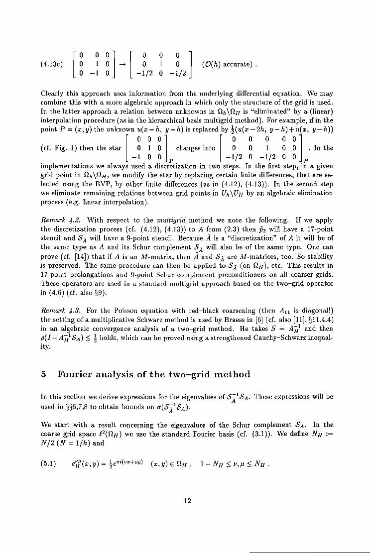
(4.13c)[ O~ -~1 ~o 1- [ 0 0-~/2 ~

(O(h) accurate) .

Clearly this approach uses information from the underlying differential equation. We maycombine this with a more algebraic approach in which only the structure of the grid is used.In the latter approach a relation between unknowns in nh\nH is "eliminated" by a (linear)interpolation procedure (as in the hierarchical basis multigrid method). For example, if in the

point P = (x, y) the unkno[wn ~(x0- h~ lY - h) is replaced [bY t(u(x0- 2h,0 Y -~) +0U1(X, y - h))

(d. Fig. 1) then the star 0 1 0 changes into 0 0 1 0 0 In the-1 0 0 p -1/2 0 -1/2 0 0 p

implementations we always used a discretization in two steps. In the first step, in a givengrid point in nh\nH , we modify the star by replacing certain finite differences, that are se­lected using the BVP, by other finite differences (as in (4.12), (4.13)). In the second stepwe eliminate remaining relations between grid points in Uh \UH by an algebraic eliminationprocess (e.g. linear interpolation).

Remark 4.2. With respect to the multigrid method we note the following. If we applythe discretization process (d. (4.12), (4.13)) to A from (2.3) then P2 will have a 17-pointstencil and SA will have a 9-point stencil. Because A is a "discretization" of A it will be ofthe same type as A and its Schur complement SA will also be of the same type. One canprove (d. [14]) that if A is an M-matrix, then A and SA are M-matrices, too. So stabilityis preserved. The same procedure can then be applied to SA (on nH), etc. This results in17-point prolongations and 9-point Schur complement preconditioners on all coarser grids.These operators are used in a standard multigrid approach based on the two-grid operatorin (4.6) (d. also §9).

Remark 4.3. For the Poisson equation with red-black coarsening (then An is diagonal!)the setting of a multiplicative Schwarz method is used by Braess in [6] (d. also [11], §11.4.4)in an algebraic convergence analysis of a two-grid method. He takes S = Ai/ and thenp(I - Ai/SA) ~ ~ holds, which can be proved using a strengthened Cauchy-Schwarz inequal­ity.

5 Fourier analysis of the two-grid method

In this section we derive expressions for the eigenvalues of SiISA. These expressions will beused in §§6,7,8 to obtain bounds on a(SiISA).

We start with a result concerning the eigenvalues of the Schur complement SA. In thecoarse grid space .e2(nH) we use the standard Fourier basis (d. (3.1)). We define NH :=N/2 (N = l/h) and

(5.1) e';f(x, y) = ~e7l"i(vX+ltY) (x, y) E nH, 1 - NH ~ v,p ~ NH .

12

Lemma 5.1. The Fourier mode e';r (1- NH ~ v,j.L ~ NH, (v,j.L) f; (0,0» is an eigenvectorof SA with corresponding eigenvalue the harmonic mean ofd~lJ,d~lJ,d~lJ,d~1J (cf. (3.11», i.e.:

(5.2) SAevlJ - H(dlJlJ dVIJ dVIJ dVIJ)eVIJH- 1'2'3'4 H'

Proof. If A: .e2(nh) ~ .e2 (nh) would be nonsingular then the formula

immediately yields SAl = [0 I]A- 1 [ ~ ]. Fourier transformation then results in the har­

monic mean as in (5.2). However, A is singular with Ker(A) = 1 h and a special treatment ofthe vector I h is needed. Define r2 := [- A2"l All I] and note that ff I H = I h (d. Remark4.1) and therefore rz(][ t) c ][ ii. We use the (generalized) inverse SAl: ][ ii ~ ][ ii (d.Remark 4.1). Now define W: :0: t ~ .eZ(nh) by

W S-l- + A-I:= pz A rz PI 11 T1

(pz, TbP1 as in (4.2». Note that W is well-defined due to rz(][ t) c :0: ii. A simple calculationshows that AW = I,ll /;.

Using [ ~ ] ][ ii c ][ t we see that W [ ~] : :0: ii - .e2(nh) is well-defined. From the

definition of W we now conclude that [0 I]W [ ~ ] = SAl. Note that1:0: if

(5.3) [0 I]e~1J = [0 I]e~'1J = [0 I]e~IJ' = [0 I]e~'IJ' = e';r (1- NH ~ v,j.L ~ NH).

We take a Fourier mode e';r E 1 ii, i.e. (v, It) f; (0,0). Using [ ~ ] = [0 IV = HO 1]* and

(5.3) we see that

From AW = Ill/; we have A lVe~1J = e~1J and thus W e~1J = 1/ d~1Je~1J + Q VIJ I h for a certain

Q VIJ E C. Similar relations hold for e~'IJ, e~IJ' and e~'IJ'. Combining this with (5.4) we get

W [0] VIJ 1 ( /dvlJ VIJ /dvlJ V'IJ /dvlJ VIJ' /dvlJ V'IJ') f3 1I eH = 4 1 1 eh + 1 2 eh +1 3 eh + 1 4 eh + VIJ h

for a certain f3vlJ E C. Using (5.3) and [0 1]][ h = I H we have

13

Finally, because [0 f]W [ 0 ] =SAl: ] if -+ ] if, we conclude that f3VJ.L = 0 andf I] ~

o

Remark 5.2. In the multigrid literature there are other approaches in which the Schur comple­ment plays an important role (d. §4). In these approaches the Schur complement SA = r2Ap2(d. (4.5d)) is approximated by the coarse grid stiffness matrix. In Fourier space this meansthat the harmonic average H(d~J.L,d~J.L,d~J.L,d~J.L) is approximated by (an approximation of)d~J.L. In our approach we approximated SA by SA = r2Ap2 (d. (4.11b)), thus using infor­mation from AI { VI' d V'I' VI" V'I"}' This leads to a better approximation of the harmonic

span eh ,eh ,eQ.-. ,ehaverage as can be seen from l'ig. 2,4,5.

To be able to apply Fourier analysis to SA = r2Ap2 we first introduce some notation. Asdiscussed in §4 we have modified equations [All An] in the grid points of nh\nH. The gridpoints of nh\nH are divided in three sets:

(5.5a)

(5.5b)

(5.5c)

n~l) = {(x, y) E nh\nH Iy= kH, k E .tz}

n~2) = {(x, y) E nh\nH I x = kH, k E iZ}

n~3) = (nh\nH )\(n~l) u n~2)) .

Note that for given j E {1, 2, 3} A has a constant difference star in the points of n~), thus

for a suitable r('j}, independent of (x, y) E n~) we have

In Lemma 5.3 it is shown that the eigenvalues of SA can be expressed in terms of these r(j)and the eigenvalues of A.

Lemma 5.3. For (v,p,):j:. (0,0) with 1- NH ~ v,fl ~ NH the following holds

(5.7) S _eVJ.L - {dV/L + l(rV/L + rVJ.L)(dV/L dVJ.L) + 1 (rV/L rV/L)(dV/L dV/L)}eV/LA H - 1 4 (1) (2) 4 - 1 4" (1) - (2) 2 - 3 H'

Proof. We use the Galerkin property SA = r2Ap2, with r2 = [0 f] and P2 = [ -Alf A12 ].

The Fourier transform ofp2 is equal to the transpose of the Fourier transform of H-Ai2All f].The latter restriction operator has a constant (17-point) difference star. From this we seethat (d. [10] §8.1.2)

14

,We take a fixed (v, J1) f= (0,0) with 1 - NH ~ v, J1 ~ NH and write P2e'Jr = al e~1J. +a2e~ J.t +

vJ.t' v' J.t'a3eh + a4eh •

N t th t v'J.t - VJ.t v/IJ.. - ( 1)i VIJ. . . - 1 2 3o e a eh InH - eh InH , eh In~) - - eh In~)' J - , , .

Similar relations hold for e~J.t' and e~'J.t/. This yields, with n1°) := nH and n~) as in (5.5),the following:

(5.8a)

(5.8b)

(cf.(5.6))

On the other hand we have

Combining this with (5.8) yields the following equations for the unknowns all a2, a3, a4:

[

1 1 1 1 ] [ al ] [ 11 -1 1 -1 a2 = 1 - 'W1 1 -1 -1 a3 1-'(2)1 -1 -1 1 a4 1 _ ,vJ.t

(3)

The matrix above has orthogonal columns. Inverting the matrix yields

(5.9)

The Fourier transformation yields

15

4

with eigenvalue ~I/p. = L d?aj. Using (5.9) we geti=1

~I/p. = d1 +HT(D + T(~)(d~P. - d~P.) + HT(D - Tm)(d~p. - d~P.)

+~T(~((d~P. + d~P.) - (d~P. + d~P.)) .

Finally, note that the last term in the right hand side is equal to zero due to (3.3). 0

Expressions for the T(~, j = 1,2, used in Lemma 5.3 are given in Lemma 5.4 below.

Lemma 5.4. If [All Ad is obtained by a "discretization" process as in (4.12), (4.13)then the following holds. With

(5.10) /I/p. := 1 - cos(v1rh) cos(Jl1rh) = 2(s~c~ +s~c~) E [0,1]

we have the following expressions for Tm (j = 1,2):

(5.lIa) T(;} = {4ah(s~ + s~c~(c~ - s~)) + a1/J1/ +(1- a)(1/Jp. + /1/p.(1-1/Jp.))}/(2ah + 1)

(5.lIb) T(~ = {4ah(s~ + s~c~(c~ - s~)) + a(1/J1/ + /1/p.(1-1/J1/)) + (1 - a)1/Jp.}/(2ah + 1) .

Proof. The result in (5.lIb) is a direct consequence of the definition of A1nC2) as in (4.12) andthe following equalities: h

[ -~8 0 -3/4 0 -1/8 ]0 2 0 I/p. 2 2 2 2 2 I/Il-o eh = 4(sp. +SI/CI/(Cp. - sp.))eh ,

-1/8 0 -3/4 0 -1/8

[ -~4 0 -1/4 0

~ ] eh" = (>p" +7""(1 - >p"1leh" ,0 1 0-1/4 0 -1/4 0

[~0 0]1 I/p. I/p.

Allln~2) = diag(2ah + 1) .~ eh = 1/Jp.eh ,-1

Using similar arguments the result in (5.lIa) can be proved. o

In Lemma 5.1 and Lemma. 5.3 we derived expressions for the eigenvalues of SA a.nd SA respec­tively. The influence of the discretization approach, i.e. replacing [All Ad by [All AI2],

16

is expressed through the eigenvalues T(j), j = 1,2, in Lemma 5.3. In Lemma 5.4 expressions

for these T('j} are given that correspond to our particular discretization strategy as in (4.12),

(4.13). As is shown in Lemma 4.1, there is a direct relation between u(Si1SA) and the

convergence of our two-grid method. Clearly, expressions for the eigenvalues of Si1SA are

obtained by combining the results of Lemma 5.1, 5.3, 5.4. Estimates concerning u(S~lSA)

will be given in the next three sections. In Section 6 and Section 7 we consider special cases,namely pure diffusion (§6) and pure convection (§7). In §8 we consider the general situation.

6 a(Si1SA): the special case of pure diffusion

In this section we analyze the case with £ = 00 (cr. (2.3». So the parameters a and £ vanishand only the mesh size parameter h remains. Moreover, we have a symmetric operator Ah,corresponding to the standard 5-point stencil of the Laplacian, and thus a real spectrum.

In Lemma 6.1 below we derive expressions for T({) ± T('~ (cr. (5.11» that are valid forthe general case of convection-diffusion, i.e. £ E (0,00). We will use the following rescaledreal eigenvalues (cr. (3.2)):

(6.1) 5.?:= >'?/Qh j = 1,2,3,4.

Lemma 6.1. For T(j) as in (5.11) the following holds ('rlJ/l- as in (5.10)):

(6.2a)

(6.2b)

1 (lJ/l- lJ/l-) _ {dlJ/l- 1 (dlJ/l- dlJ/l-) 1 \ lJ/l- 1 (\ lJ/l- \ lJ/l-)}j(2 +1)2 T(l) +T(2) - 1 + ;(YlJ/l- 4 - 1 - 2A 1 - 8/lJ/l- A4 - Al Qh

1( lJ/l- lJ/l-) _ 1 {dlJ/l- dlJ/l- 1 (\lJ/l- \lJ/l-)}/(2 1)2 T(1) - T(2) - -;(YlJ/l- 2 - 3 - 2 A2 - A3 Qh + .

Proof. From (5.11) we have that

+a'l/JlJ +(1- a)'l/J/l- + ~/lJ/l-{(1 - a)(1 - 'l/J/l-) +a(1 - 'l/JlJ)}

=dr/l- - ~>.r/l- + 2Qh{S~C~(c~ - s~) +s~c~(c~ - s~)} + ~/lJ/l-{(I- a)(I- 'l/J/l-) +a(l- 'l/JlJ)} .

Straightforward computations show that

and

Using these two equalities and d? = >'? +<p? in (6.3) yields the result in (6.2a).With respect to (6.2b) we note that

17

and that

(1- a)(l-1/J~) - a(l-1/Jv) = -!(<t'~~ - <t'~~) ,

2 ( 22+22(22) 22(22))_ 1 (\v~ \v~)O'.h Sv - s~ s~c~ Cv - Sv - svcv c~ - s~ - -8"YV~ A2 - A3 • o

For c --+ 00 we have d't /(20'.h + 1) --+ !).'t, -X't /(20'.h + 1) --+ !).'t and for c ! 0 we haved't /(20'.h + 1) --+ <t''t, -X't /(20'.h +1) --+ O. Using this in Lemma 6.1 immediately results in

Corollary 6.2. From Lemma 6.1 we derive the following results on c --+ 00 and for c ! 0:

(64b) 1· I(V~ v~)_ 1 ('\v~ '\v~)_.-· e':'~ 2 T(1) - T(2) - -16"YV~ A2 - A3 -. Too

(6 4) 1· 1 ( v~ + v~) _ v~ + 1 (v~ v~) _. +· c ;ft} 2 T(1) T(2) - <t'1 4"Yv~ <t'4 - <t'1 -. TO

(6 4d) 1· 1 (v~ /.I~) _ 1 (v~ v~) _. -· ;ft} 2 T(I) - T(2) - - 4"Yv~ <t'2 - <t'3 -. TO .

In the remainder of this section we consider a(S,tSA) for the case c = 00. For convenience

we rescale the eigenvalues d't with a factor 0'.;;1; then e~~ d't = ).'t holds ().'t as in (6.1)).

From Lemma 5.1, 5.3 we have that e';; ((v, Jl) :I (0,0)) is an eigenvector of SA and of SAwith eigenvalue

(6.5a)

(6.5b)

respectively. Here T~, T~ are defined in (6.4a,b) and we recall that ).~~ = 4(s~ + s~), ).~~ =( 2 2) '\ v~ _ '\ v~ '\ v~ _ '\ /.I~4 Cv + s~ ,A3 - 8 - A2 ,A4 - 8 - Al •

Lemma 6.3. The Fourier mode e';;, (v,Jl) :I (0,0), is an eigenvector of SA with eigen­value

Proof. Substitution of (6.4a,b) in (6.5b) yields the following expression for the eigenvalue:

(6.7)

18

Note (d. (3.12a,b)) that

(6.8)

(6.9) l6«X~1L - X~IL? - (X~IL - X~IL)2) + (H(X~IL, X~IL) - H(X~IL, X~IL))

= l6«X~1L + X~IL)2 - (X~IL + X~IL)2) = 0 (use (3.3)) .

Combination of (6.7), (6.8), (6.9) yields the result in (6.6). o

We see that the approximation of SA by S,4 corresponds, in terms of eigenvalues, to theapproximation of the harmonic mean H (X? ,x~IL, X~IL ,x~IL) by the eigenvalue as in (6.6).Note the similarity between (6.6) and the expression for the harmonic mean in (3.12c). Analternative approach would be to approximate SA by the discretization of the differentialoperator on the coarse grid (=: AH). In the setting here this yields the standard 5-point starof the Laplace operator, with eigenvalues 2(sin2 (v1l"h) + sin2(p7rh)) = 8(s~c~ +s~c~).

Summarizing we have the following relevant eigenvalues, denoted by {'/Il(.):

(6.1030) e'JL(SA) = H(X~lt, X~JL,x~JL, X~JL)

(6.10b) ~IIJL(S,4) = H(X~JL, X~JL) + ~/IIJL(H(X~JL, X~JL) - H(X~JL, X~IL))

(6.10c) ~IIJL(AH) = 8(s~c~ + s~c~) ,

and we are interested in ~1I1l(SA)/~IIJL(S,4) and ~IIJL(SA)/~IIJL(AH) «v,p) =I- (0,0)) . Thestrengthened CBS inequality as in [11] yields the following:

Proof. We take (v, p) =I- (0,0) and introduce the notation 1 := IIIJL_ = 2~s~c~ + s~c~~, (3 :=

2(s~c~ + s~c~). Note that 0 ::; (3 ::; 1 ::; 1 holds. Also hij := H(>.rJL ,>.?) = ~>'?>'? Astraightforward calculation shows that h14 = 2C/ +(3), h23 - h14 = 4(1-/,) and h14 /(h23 +h14 ) = ~({3 +1)/({3 + 1). Using the results in (6.10a,b) and (3.12c) we get

~IIJL(SA)/~IIJL(S,4) = 1 + (~IIJL(SA) - ~IIJL(SA))/~IIIl(S,4)

= 1 + (h h1

\ - h) (h23 - h14 )/(h14 + ~/(h23 - hI4 ))23 + 14

_ {3(1 -/)2 _.- 1 + ({3 + 1)({3 +1(2 -I)) -.1 + fC/,(3) .

19

An elementary analysis shows that for °:s: (3 :s: 'Y :s: 1, °:s: f( 'Y, (3) :s: f( 'Y, 'Y) :s: ~ holds. 0

With optimal damping we have that p(I - WoptAi/SA) :s: ~ and p(I - WoptS,tSA) :s: tand these bounds are sharp for h 1 o. In Fig. 2 we show a(Ai/SA) and a(Si1SA) forh = 1/32, Le. NH = 16 and -15:S: V,jl:S: 16 ((v,jl) f; (0,0».

'" '"

Fig 2

From the results above we conclude that a(Si1SA) is more favourable than a(AiiSA) in two

respects. Firstly, p(I - WoptSi1SA) ~ 1/7 is (significantly) smaller than p(I - WoptAiiSA) ~1/3 and secondly, we observe a clustering of the eigenvalues in a(Si1SA) close to 1. This can

be seen from Fig. 4, too. For the eigenvalues in Fig. 2 we have mean{a(Si1SA)} = 1.07 and

mean{a(Ai/SA)} = 1.42.

7 u(Si1SA): the special case of pure convection

In this section we analyze the case with E: = 0, h E (0,1], a E (0,1) (d. (2.3». We willprove a robustness result for a(S,tSA) with respect to variation in hand a. Also, to givesome further indication of the quality of SA as a preconditioner for SA, we have computeda(Si1SA) for h = 1/32 and for several values a E (0,1).

We start by noting that for E: lOwe have d? - c.p? From Lemma 5.1, 5.3 and Corol­lary 6.2 we see that eJ: «v,jl) f; (0,0» is an eigenvector of SA and of SA with eigenvalue

(7.1b) IrJVP- + L-+(lI',vp- _ t...,vP-) + l""-(lr,vp- _ Ir,vP-)..,-1 2'0..,-4 ..,-1 2'0..,-2 ..,-3

respectively. Here Td and TO are as in (6.4c,d).

Lemma 7.1. The Fourier mode eJ:, (v, It) f; (0,0), is an eigenvector of SA with eigen­value

20

Proof. Substitution of (6.4c,d) in (7.1b) yields the following expression for the eigenvalue:

cprtt +!(cprtt + ~/'lItt(cp~tt _ cp~tt))( cp~tt _ cp~tt) -l/'lI tt( cp~tt _ cp~tt)2

= cp~tt + ~cp~tt(cp~tt _ cp~tt) + !/'lIttH(cpt _ cp~tt)2 _ (cp~tt _ cp~tt)2) .

Note that (d. (3.12a,b))

H( IItt IItt) IItt 1 IItt( IItt IItt)CPl ,CP4 = CPl + "2CPl CP4 - CPl ,

and

H(cp~tt - cp~tt)2 _ (cp~tt _ cp~tt)2) + (H(cp~tt,cp~tt) _ H(cp~tt,cp~tt))

= H(cp~tt + cp~tt)2 - (cp~tt + cp~tt?) = ° (use (3.3)) .

Note the similarity between the expressions in (6.6) and in (7.2).Below we compare ~lItt(SA):= H(cp~tt,cp~tt,cp~tt,cp~tt)with

~lItt(S _) .- H( Utt II tt ) t (H( IItt II tt ) H( IItt Utt)).. A·- CPt, CP4 + "2/'lItt CP2' CP3 - CPt, CP4 •

o

We are interested in estimates for ~lItt(SA)/~lItt(SAJ that are uniform in hand a. Such esti­mates are given in Theorem 7.2 below, where (for ease) we consider the inverse eigenvaluesett(S)J/~lItt(SA).

Theorem 7.2. The following holds for (v,j.l) =j:. (0,0):

(7.3a) Re(~lItt(SA)/~lItt(SA)) 2: !(7.3b) 1~lItt(SA)/~lItt(SA)1 ~ 2 .

Proof. If we substitute H(cprtt,cp't) = cprttcp't, (i,j) E {(2,3),(1,4)}, in the expression for~lItt (SA) above, then we get

4

qlltt := ~lItt(SA)/~lItt(SA) = ~((1 - ~/'lItt)cp~ttcp~tt + !/'lIttcp~ttcp~tt) L l/cp't .j=l

Note that cp~tt + cp~tt = cp~tt + cp~tt = 2, /' lItt E [0,1]; using (3.7c) we see that

Re(qlltt) = !Re{((1- !/'lItt)cprttcp~tt+ !/'lIttcp~ttcp~tt)((cprttcp~tt)-l + (cp~ttcp~tt)-l)}

= !Re{l + (1 - !/'lItt)cprttcp~tt( cp~ttcp~tt)-l + !/'lIttcp~ttcp~tt(cprttcp~tt)-l}

= ! + ~(1- !/'lItt)Re{cp~ttcp~tt(l/cp~tt + l/cp~tt)}

+l/'lIttRe{cp~ttcp~tt(l/cp~tt + l/cp~tt)} 2: ~ .

21

This proves (7.3a). We now consider (7.3b):

(7.4)

IqlllLl = ~I(ip~lLip~1L + ~'IIIL( ip~lLip~1L _ ip~lLcp~IL))( ip~lLip~IL)-1

+( ip~lLcp~1L + (1 _ ~'IIIL)( ip~lLip~1L _ ip~lLcp~IL))(ip~lLip~IL)-11

::; 1 + !'lIlLlip~lLip~1L _ ip~lLcp~lLllcp~lLip~ILI-1

+1(1 I )1 IIIL IIIL IIIL IIILII IIIL IIILI-I2" - 2"11I1L ipl cp4 - ip2 ip3 ip2 ip3 .

Also we have

For the denominators in (7.4) we use that

(7.6) lip~lLip~1L1 = Icp~lLllcp~1L1 ~ Re(cp~IL)Re(cp~lL) = 4(as~ +(1 - a)s~)(ac~ +(1- a)c~)

~ 4a(1 - a)(s~c~ + s~c~) = 2a(1 - a)-y1l1L ,

and

(7.7) lip~lLip~1L1 ~ Re(ip~IL)Re(cp~lL) = 4(ac~ +(1- a)s~)(as~+(1- a)c~)

~ 4a(1 - a)(c~c~ + s~s~) = 4a(1- a)(1 - ~'IIIL) .

Using (7.5), (7.6) and (7.7) in (7.4) yields the result in (7.3b). o

From Theorem 7.2 it follows that cr(SiISA) lies in a bounded domain in the complex righthalf-plane away from the imaginary axis. Moreover, this domain is independent of the pa­rameters h and a, i.e. we have a robustness result w.r.t. variation in hand a.In Fig. 3 below we show cr(SiISA), in the complex plane, for h = 1/32 and for several values

a E (0,1); due to symmetry it is sufficient to consider a E (0, ~].

With respect to the results in Fig. 3 we remark the following. Because SilSA is real there

is symmetry w.r.t. the real axis. For a = ~ eigenvalues coincide due to symmetry. From theresults in Fig. 3 it is clear that the estimate in (7.3a) is sharp.We briefly comment on the two clusters of eigenvalues for a small (a = 10-3 ,10-2). Fora = ° SA has kernel span{e~ I J1, = O}, and it is easy to verify that for J1, # °wehave ~IIIL(SA) = elL(SAJ For a small the cluster of eigenvalues with real part ~ 1 (~2)

corresponds to the eigenfunctions e~ with JL # °(J1, = 0). As might be expected, the ap­proximation of ~IIIL(SA) by ~1I1L(S.-4) is worse for the eigenvalues which are perturbations (fora 10) of the zero eigenvalues of SAla=O'Finally we note that in all cases in Fig. 3 we observe a clustering of eigenvalues in some(small) neighbourhood of 1 (as in §6). Further calculations show that for a = 0.3,0.4,0.5about half of the eigenvalues lies in the domain [0.85,1.2] X [-0.2,0.2] with area 0.14, whereasthe convex hull of cr(Si1SA) has an area ~ 1.1.

22

0.015r---~---~--~---~--~-----, 0.15r---~---~--~---~--~--___,

0.01

0.005

-0.005

-0.01

!....

I"...i

0.1

0.05

-0.05

-0.1

A+ +

: ++ +

lJ=+ ++ ++ ++ +++ ++ +~.

-o.01~.':-.---!---"'1'::.2--"""'1'::.'--"""'1'::.•--"""'I'::.•-----! -o·,~.I:-.-----,!---..,,'::.2--......,l'::.•--......,,'=.•--......,,'=.•------:

a 0.001 a =0.01

O.•r---~--~_:_...,.....,....,---.,.....--~--...,

0.4

0.'

-0.'

-0.'

-o~.':.•---~---;,'=.•--'-...:....-'-;,~.•------;,';;.•------;,';;.•:--~

a 0.1 a 0.2

+ ++

++ +

0.'

0.'

-0.'

-0.'

O.•,---~---+~+-+-+-"..,...,T+..., •.-+~-+~--~-----,+ +... +t ........ ++

~~~~..~: { + ++ i<++ +.. ::. ++. +.+'+4. t.+ ..t t:: :/.. \.. .. :+..........++.:

tttk:{:~::++ .. +.++++.+.. ++ ..

;\.+ + ..•• u* * +'#.-1'+ .. ++.. ••+++~+++::.t++.." ++ ..•~:::+..+++++ .+.+ .... +++1 .. ...... .. ..1 ••• .. .. .+ .. .. ..+::+:+++~.+ f ++ ++.+#++++1+ +~

~+ +++i." +.+++$. 1:: ... \ ..

...+ .. +t: ++ ..

.. .. .. +.... ....".()·8.':-.-----.,!---..,,'::.•---',L.•..L--'--,~.--......,,~.•-----J

a 0.3Fig 3

a = 0.5

In this section we analyze the general situation with (Xh E (0,00), h E (0,1], a E (0,1). Inprinciple we follow the approach as in §§6,7. However, the analysis is more technical becauseour estimates here have to be uniform in three parameters.

23

Also, to illustrate the dependence of a(Si1SA) on the convection/diffusion ratio we havecomputed a(Si1SA) for h = 1/32, a = 004 and for several values Qh E (0,00).

From Lemma 5.1,5.3 we see that e'];, (v,p) t= (0,0), is an eigenvector of SA and of SAwith eigenvalue

(8.1a) C'J.l(SA) := H(d~J.l, d~J.l, d~J.l, d~J.l) and

(8.1b) ~VJ.l(SA) := d~J.l + ~(I(i) + 1(~)(d~J.l - d~J.l) + ~(I(i) - 1(~)(d~J.l - d~J.l)

respectively. In (8.1b) we have I(i) ± I(~ as in Lemma 6.1.Based on the expressions for I(i) ± I(~ we define the following:

(8.2) g":J.l '= 1 ,~J.l + !l·FJ.l = d~J.l _ l' VJ.l J' - 1 2 3 4J . 2 A J T' J J. 2 AJ' -",.

Then we have

(8.3a)

(8.3b)

1( VJ.l VJ.l) _ (VJ.l 1 (VJ.l VJ.l))/(2 1)2 1(1) +1(2) - g1 + ;(YVJ.l g4 - g1 Qh +

We use (8.2), (8.3a,b) to rewrite the expression in (8.1b). A straightforward calculation thenyields the following expression for ~VJ.l(SA):

(8Aa) ~VJ.l(SA) = T1+T2 +T3 ,with

(8Ab) T1 = H(g~lt,g~J1) + !'VJ.l(H(g~lt,g~lt) - H(g?,g~J.l))

(8Ac) T2 = !.x? + ~(1- !'VJ.l)(.x~J.l - .x~J.l)g? /(2Qh + 1)

(8Ad) T3 = ~,vJl{(2Qh + l)(A~Jl - .x~Jl) - !(.x~Jl - .x~Jl)(g~J.l - g~Jl)} /(2Qh + 1) .

The term T1 is of the same form as in Lemma 6.3 and in Lemma 7.1. For Qh 1°the term T1

is 0(1) whereas T2 ,T3 are O(Qh). In the Lemmas 8.2,8.3,804 below we will prove that for(v, p) t= (0,0) we have Re(Tj/~VJl(SA)) ~ 0, j = 2,3, and Re(Td~VJl(SA))~ ~. Therefore westate the following

Theorem 8.1. For (v,p) t= (0,0) the following holds:

Proof. Direct consequence of (8Aa) and Lemma 8.2, 8.3, 804.

Lemma 8.2. With T2 as in (8.4c) we have the inequality

24

o

Proof. First notice that Re(l/d't) ~ 0 and therefore Re(l/e'JL(SA)) ~ O. Also we haveA? ~ 0, (A~JL - A~JL) > 0, (1 - !'YVJL) > O. From this we see that for proving the result in(8.6) it is sufficient to prove that

(8.7) Re(g?d?) ~ 0 for j = 1,2,3,4.

The inequality in (8.7) follows from

Lemma 8.3. With Ta as in (8.4d) we have the inequality

(8.8) Re(Ta/~VJL(SA)) ~ 0 for (v, JL) -::J (0,0) .

Proof. We begin with rewriting Ta as T3 = ~'YVJL(TJl) +TJ2))/(2ah + 1),

TJl) := 2ah(A~JL - A~JL) - HA~JL _ A~JL)2

TJ2) := (A~JL _ A~JL) _ !(A~JL _ A~JL)(<p~JL _ <p~JL) .

Because Re(I/~VJL(SA)) ~ 0 holds it is sufficient to prove

(8.9a) T(l) > 03 -

(8.9b) Re (TJ') (t, 1/di")) ,,0.

Using the definition of A? and introducing p := c~ - s~, q := c~ - s~ (p, q E [0,1]) we get:

TJ1) = 8a~(p +q) - 4a~(p _ q)2

~ 4aH2(p+ q) - (p+ q?} = 4a~(p+ q)(2 - (p+ q)) ~ O.

So (8.9a) holds. For TP) we have

TJ2) = 4ah(P+ q) - 2ah(P _ q)(<p~JL _ <p~JL)

= 2ahP(2 - (<p~JL _ <p~JL)) +2ahq(2 _ (<p~JL _ <p~JL))

So for (8.9b) to hold it is sufficient to prove

(8.10) Re (<pi" (~ lId?)) ,,0 for j = 2,3.

25

For k E {I, 2, 3, 4} we have

Re(<p? /d~lJ.) = Id~IJ.I-2Re(<p?(.'\~1J. + ~~t))

~ Id~IJ.I-2Re(<p?~~IJ.) ~ 0 (use (3.7a)) .

From this it follows immediately that the estimate in (8.10) holds.

Lemma 8.4. With T1 as in (8.4b) we have the inequality

(8.11) Re(Ttle'IJ.(SA)) ~ 1 for (v, p,) i (0,0) .

o

Proof. First note that H(g?,gZIJ.) = (2Qh + l)-lg?gZIJ. for (j,k) E {(2,3),(1,4)} and thus

So for (8.11) to hold it is sufficient to prove

(8.12a) Re (~F~~:) ~ t for (j, k) E {(2, 3), (l,4)} , and

(8.12b) Re(~~:~F) ~O, Re(~~:~~:) ~O.

We first consider (8.12a). Take (j, k) E {(2, 3), (1,4)} and note that gflJ. = ~(drlJ. + <p?) andthus

(8.13)

Now use that for i E {1,2,3,4}

and

Re(<p?<p~JLd'td~JL) = >.? >.~JLRe(<p?<p~JL) + >'?I<p~JLI2Re(<p?)

+>.~IJ.I<p?12Re(<p~JL) + 1<p?121<p~JLI2 ~ 0 (use (3.7b)) .

26

The latter two inequalities and (8.13) together imply the result in (8.12a).

We now consider the first inequality in (8.12b). The second result in (8.12b) can be provedsimilarly.

Note that for j E {2,3} we have

Re(g?g~lLd?) = Re((!>,~1L + <p~IL)(!A~1L + <p~IL)(A? +IP?»

= !AIIIL AIlIL AV.IL + !AIIIL AIlILRe(Il'JV.IL ) + !A IIIL AV.ILRe((l'JIIIL)4 1 4 J 4 1 4 TJ 2 1 J T4

+!A~ILA?Re(<p?) + !A~ILRe(<p~ILIP?) + !A~ILRe(<p~IL¢t)

+Aj Re( <p~1L <p~IL) +Re( <p~1L <p~IL<P;IL) ,

and all the terms in the right hand side are positive due to A? ~ 0 and the results of Lemma3.1. Using this in (8.14) we see that the first inequality in (8.12b) is valid. 0

The results in Lemma 8.2,8.3,8.4 imply Theorem 8.1 and thus we have proved that a(SA1SA)lies in the half pla.ne {z Eel Re(z) ~ D. In Theorem 8.6 below we prove tha.t a(SA1SA) isbounded uniform in h, a, E.

Lemma 8.5. For (v, It) i- (0,0) the following inequality holds:

Proof. We rewrite (8.1b) as follows

~1I1L(SA) = d? + ~T(i){(d~1L + d~lL) - (d~1L + d~lL)} + ~T(~{(d~1L + d~lL) - (d~1L + d~lL)}

= d~1L + T(i){20'h(C~ - s~) +a(1- "pll)} +T(~{20'h(C; - s;) +(1- a)(l- "p1L)} .

So

We first consider the term IT(i)/d~lLl. With ~~IL := 40'h(S~+s~c~(c~ - s~» ~ A~IL we get (cf.(5.11a) for T(i)

27

A similar computation for ITmld~1L1 yields

Using these estimates in (8.16) results in

(8.17)

Now note that

(ah +a(l - a»)-yvlt = 2ah(s~c~ + s~c~) +a(l - a)(2s~c~ +2s~c~)

::; 4ah(s~ + s~) +2as~ +2(1- a)s~ = Re(d~lL) .

Using this in (8.17) we get

Theorem 8.6. For (v,p) -=I- (0,0) the following estimate holds:

o

(8.18)

Proof. The result in (8.18) is a consequence of Lemma 3.2 and Lemma 8.5:

4

I~VIL(S.4)/elL (SA)1 = tl~VIL(S.4)(L 1Id?)1j=l

4

::; tl~VIL(S .4)ld~lLl(l +L Id~1L Id?l)j=2

::; ~4(1 +2)2(2 +V2) + 1) = 2(1 + )2(2 +V2» . o

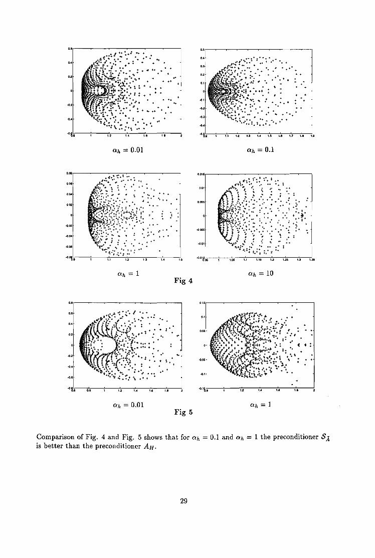
From Theorem 8.1 and Theorem 8.6 it follows that a(Sj"lSA) lies in a bounded domain in thecomplex richt half-plane away from the imaginary axis. Moreover this domain is independentof the parameters c, h, a, i.e. we have a robustness result w.r. t. variation in c, hand a.In Fig. 4 below we show a(Sj"lSA), in the complex plane, for h = 1/32, a = 0.4 and for

several values of ah (= clh). In Fig. 5 we give analogous results for a(Aj/SA) (AR: standardcoarse grid discretization).In Fig. 4 we see that the convex hull of a(Sj"lSA) shrinks if ah increases (i.e. more diffusion).Also, as in §§6,7 we observe a clustering of eigenvalues in a small neighbourhood of 1.

28

-O·~.'='.--7--:,:'::.'--:';';.2:---;':,.•;----:,.,-;---;',.';',--;,';;.•--;,:'::.7'----:';';.•;---7...

+ +

+ +

+ ++ ..

+++ ++

• +• +

.. ++

+ .... ++

+ ++: + ++

0.'

0.2

O.•.---~--~---~--~--~----,

-O·8.1::.---~---:,:,::.2--'-----:,:,:.•,------:,:,:.•,------:,:,::.•,------!

-0.'

-0.'

0.1

0.01

-0,01

0.005

O.Ol'r--~--~-~--~--~-~--~----'

-0.005

+..+

+ + +

+ + +++ + +

++ + ...

++ + +

..+ +

+ ...+ ...

++

+ + ++

++ .. +

+ +

++

+ +

...... ... ....+

0.08

0."

0."

0.08r---~---~____:____:~---~--~---,

-0.04

,(1.08

·0.02

'O.OB.'=".-----:c----:'1.':-,---'-------:',.':-.------:',.':-.------:',-=-.-----:'.6 -o.0~..!:;---7---;,.~05;---'1;';.,;-----:,~.'~6---;',.';;-'----;-1.'~6;-----:,:,::.•,----71.3"

10Fig 4

O.•.--~--~--~--~--~--~--, 0"6r---~---~--~---~--~-----'

..

..

+ +

+ +

-O·8.1::.---;:0'=.•---7---:,'=.•'---:,:':.•---:,:'::.•,---:,:'::.•,----! -O·'~.'='.-----:C---":'U'::---":".~.----;,.'=.----;,,=.•--~

0.01 1Fig 5

Comparison of Fig. 4 and Fig. 5 shows that for ah

is better than the preconditioner AH.0.1 and ah 1 the preconditioner SA

29

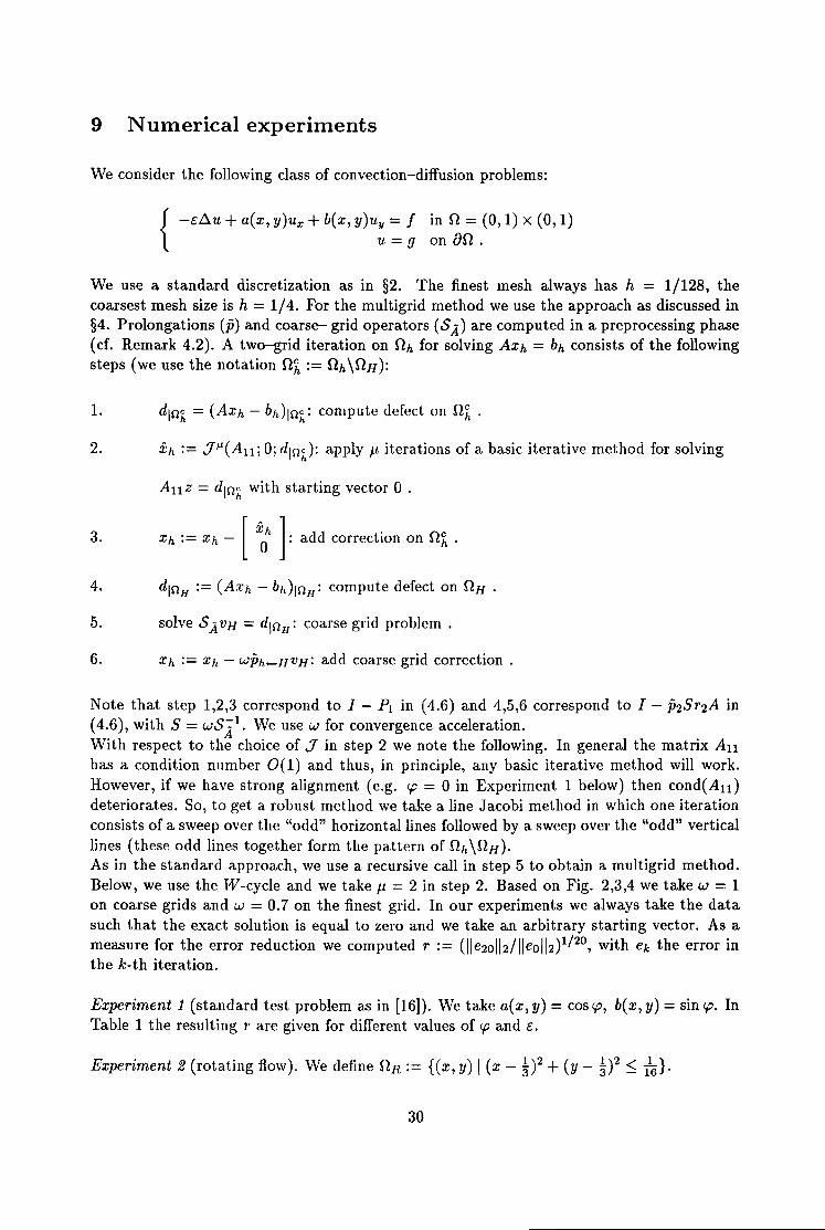
9 Numerical experiments

We consider the following class of convection-diffusion problems:

{-£~u +a(x, y)ux +b(x, y)uy = f in n = (0,1) x (0,1)

u = 9 on an.

We use a standard discretization as in §2. The finest mesh always has h = 1/128, thecoarsest mesh size is h = 1/4. For the multigrid method we use the approach as discussed in§4. Prolongations (p) and coarse- grid operators (SA) are computed in a preprocessing phase(cr. Remark 4.2). A two-grid iteration on nh for solving AXh = bh consists of the followingsteps (we use the notation nh:= nh\nH):

2. Xh := .JJ-£(An ; 0; d lni): apply It iterations of a basic iterative method for solving

Anz = dlnh with starting vector 0 .

3. Xh := Xh - [ XOh ]: add correction on nh.

5. solve SjjVH = d\nH : coarse grid problem.

6. Xh := Xh - WPh+-HVH: add coarse grid correction.

Note that step 1,2,3 correspond to 1- Pl in (4.6) and 4,5,6 correspond to I - P2Sr2A in(4.6), with S = wSil. We use W for convergence acceleration.With respect to the choice of .J in step 2 we note the following. In general the matrix Anhas a condition number 0(1) and thus, in principle, any basic iterative method will work.However, if we have strong alignment (e.g. c.p = 0 in Experiment 1 below) then cond(An)deteriorates. So, to get a robust method we take a line Jacobi method in which one iterationconsists of a sweep over the "odd" horizontal lines followed by a sweep over the "odd" verticallines (these odd lines together form the pattern of nh\nH).As in the standard approach, we use a recursive call in step 5 to obtain a multigrid method.Below, we use the W-cycle and we take It = 2 in step 2. Based on Fig. 2,3,4 we take W = 1on coarse grids and w = 0.7 on the finest grid. In our experiments we always take the datasuch that the exact solution is equal to zero and we take an arbitrary starting vector. As ameasure for the error reduction we computed r := (1Ie20112/lleoI12)1/20, with ek the error inthe k-th iteration.

Experiment 1 (standard test problem as in [16]). We take a(x,y) = cos<p, b(x,y) = sin<p. InTable 1 the resulting r are given for different values of <p and c.

Experiment 2 (rotating flow). We define nR := {(x, y) I (x - ~)2 + (y - ~? :::; 116 }.

30

a(x, y) = sin(1r(Y - ~)) cos(1r(x - ~)) if (x, y) E S1R , and zero otherwise j

b(x, y) = - cos(1r(Y - ~)) sin(1r(x - ~)) if (x, y) E S1R , and zero otherwise.

The results are given in Table 2.

Experiment 3 (as in [20]). We take a(x, y) = (2y - 1)(1 - x 2 ), b(x, y) = 2xy(y - 1). Theresults are given in Table 3. In Table 3 we also show results for the two-grid method (TG).

c c.p 0 1r/8 21r/8 31r/8lOU 0.24 0.24 0.24 0.24

10-'1 0.24 0.24 0.24 0.2410-4 0.27 0.30 0.29 0.3010-6 0.30 0.31 0.30 0.31

Table 1

c l'

lOU 0.2510-2 0.2410-4 0.3010-6 0.31

Table 2

c TG W-cyclelOU 0.23 0.24

10-2 0.22 0.2410-4 0.30 0.3010-6 0.34 0.34

Table 3

These results show the robustness of our method with respect to both the convection/diffusionratio and the flow direction.

References

1. Axelsson, 0., Vassilevski, P.S.: Algebraic Multilevel Preconditioning Methods. I. Numer.Math. 56, 157-177 (1989).

2. Axelsson, 0., Vassilevski, P.S.: Algebraic Multilevel Preconditioning Methods. II. SIAMJ. Numer. Anal. 27, 1569-1590 (1990).

3. Bank, R.E.: A comparison of two multilevel iterative methods for nonsymmetric andindefinite elliptic finite element equations. SIAM J. Numer. Anal. 18, 724-743 (1984). ,

4. Bank, R.E., Benbourenane, M.: A Fourier analysis of the two-level hierarchical basismultigrid method for convection-diffusion equations. In: Proceedings of the Fourth In­ternational Symposium on Domain Decomposition Methods for Partial Differential Equa­tions, 1-8, SIAM, Philadelphia (1991).

5. Bank, R.E., Benbourenane, M.: The hierarchical basis multigrid method for convection­diffusion equations. Numer. Math. 61, 7-37 (1992).

6. Braess, D.: The convergence rate of a multigrid method for solving the Poisson equation.Numer. Math. 37,387-404 (1981).

7. Bramble, J., Pasciak, J., Xu, J.: The analysis of multigrid algorithms for nonsymmetricand indefinite elliptic problems. Math. Compo 51,389-414 (1988).

8. Brandt, A., Yavneh, I.: Accelerated multigrid convergence and high-Reynolds recirculat­ing flows. SIAM J. Sci. Comput. 14,607-626 (1993).

9. Hackbusch, W.: Multigrid convergence for a singular perturbation problem. Lin. Alg.Appl. 58, 125-145 (1984).

10. Hackbusch, W.: Multigrid Methods and Applications. Springer, Berlin Heidelberg NewYork (1985).

H. Hackbusch, W.: Iterative Losung grosser schwachbesetzter Gleichungssysteme. Teubner,Stuttgart (1991).

31

12. Kuznetsov, Y.A.: Multigrid Domain Decomposition Methods. In: Proceedings of theThird International Symposium on Domain Decomposition Methods for Partial Differen­tial Equations, 290-313. SIAM, Philadelphia (1990).

13. Reusken, A.: Multigrid with matrix-dependent transfer operators for a singular pertur­bation problem. Computing 50, 199-211 (1993).

14. Reusken, A.: Multigrid with matrix-dependent transfer operators for convection-diffusionproblems. In: Multigrid Methods IV (P. Hemker and P. Wesseling, eds.), 269-280.Birkha.user, Basel (1994).

15. Reusken, A.: A new robust multigrid method for 2D convection- diffusion problems.RANA 94-04, submitted (1994).

16. Wesseling, P.: An Introduction to Multigrid Methods. Wiley, Chichester (1992).17. Xu, J.: Iterative methods by space decomposition and subspace correction. SIAM Review

34, 581-613 (1992).18. Yserentant, H.: Hierarchical bases of finite element spaces in the discretization of non­

symmetric elliptic bounda.ry value problems. Computing 35, 39-49 (1985).19. Yserentant, H.: Old and new convergence proofs for multigrid methods. Acta Numerica,

285-326 (1993).20. Zeeuw, P.M. de: Matrix-dependent prolongations and restrictions in a blackbox multigrid

solver. J. Comput. Appl. Math. 33,1-27 (1990).

32