fracture patterns in non-plane strain boudinage · 2013-02-18 · 1 fracture patterns in non-plane...

JOURNAL OF GEOPHYSICAL RESEARCH, VOL. ???, XXXX, DOI:10.1029/,

Fracture Patterns in Non-Plane Strain Boudinage -1

Insights from 3D Discrete Element Models2

Ste!en Abe1, Janos L. Urai

1,2and Michael Kettermann

1

S. Abe, RWTH Aachen University, Geologie-Endogene Dynamik, Lochnerstrasse 4-20, 52056

Aachen, Germany, ([email protected])

J.L. Urai, RWTH Aachen University, Geologie-Endogene Dynamik, Lochnerstrasse 4-20, 52056

Aachen, Germany, ([email protected])

M. Kettermann, RWTH Aachen University, Geologie-Endogene Dynamik, Lochnerstrasse 4-20,

52056 Aachen, Germany, ([email protected])

1Structural Geology - Tectonics -

Geomechanics, RWTH Aachen University

2German University of Technology

(GUTech), Muscat, Sultanate of Oman

D R A F T November 20, 2012, 6:07pm D R A F T

X - 2 ABE ET AL.: 3D BOUDINAGE

Abstract.3

We use 3D Discrete Element Method (DEM) simulations to model the evo-4

lution of boudin structures in a layered material under non-plane strain con-5

ditions. As the models are shortened perpendicular to the layer orientation6

they are extended at di!erent rates in the two layer-parallel directions. The7

particular emphasis of the study is on the orientation of fractures between8

the boudin blocks. The results show that the fracture orientation distribu-9

tion is closely connected to the ratio of the two layer parallel extension rates.10

The anisotropy of the fracture orientation distribution increases systemat-11

ically from no anisotropy at isotropic layer-parallel extension to a highly anisotropic12

distribution in case of uni-axial extension. We also observe an evolution of13

the anisotropy of fracture orientation distribution with increasing deforma-14

tion in each individual model from a high initial anisotropy towards a value15

characteristic for the ratio of the layer-parallel extension rates. The obser-16

vations about the relation between the strain ratios and the fracture patterns17

do have the potential to serve as the basis for a new method to analyze strains18

in naturally boudinaged rocks.19


ABE ET AL.: 3D BOUDINAGE X - 3

1. Introduction

Boudins are relatively common structures in mechanically layered rocks which have20

been extended in a layer-parallel direction. They have been described in detail by, for21

example, Ramberg [1955]; Ramsay and Huber [1987]; Twiss and Moores [2007]; Goscombe22

et al. [2004]. The basics mechanisms governing the evolution of boudinage structures23

have been investigated by a wide range of numerical and analogue models (Mandal and24

Khan [1991]; Bai and Pollard [1999]; Bai et al. [2000]; Mandal et al. [2000]; Passchier and25

Druguet [2002]; Li and Yang [2007]; Iyer and Podladchikov [2009]; Maeder et al. [2009];26

Zulauf et al. [2009, 2010]; Abe and Urai [2012]) and are thought to be reasonably well27

understood. Based on this, the shape and orientation of the boudins is often seen as28

an indicator of the stress and strain or strain rate conditions which have been acting on29

the layered rocks at the time the boudins were formed (Goscombe and Passchier [2003];30

Maeder et al. [2009]).31

Most information which is available about the geometry of boudins, particularly at the32

outcrop scale, is in 2D. An overview over the wide range of boudin types observed in 2D is33

given by Goscombe et al. [2004]. However, much less is known about the 3D geometry of34

boudin structures. In some cases the outcrop conditions are favourable enought to enable35

field observations of the boudin geometries in 3D, for example in the case of boudinaged36

pegmatites in a marble matrix Schenk et al. [2007] and in silicicalstic rocks exposed at the37

SW coast of Portugal Zulauf et al. [2011a]. More comprehensive 3D data is available at38

the large scale from seismic images of boudinaged carbonate or anhydrite stringers in salt39

bodies (van Gent et al. [2011]; Strozyk et al. [2012]). Additional information on the shape40



and the evolution of boudins in 3D has been available recently from analogue experiments41

Zulauf et al. [2009, 2010, 2011b]; Kettermann [2009]. To gain additional insights into42

the range of boudin geometries expected in 3D we have performed a series of numerical43

experiments to study the influence of stress and strain conditions on the 3D fracture44

patterns in boudinaged layers. The work is particularly focused on the investigation of45

the evolution of boudin structures under non-plane strain conditions because significant46

deviations from the 2D models are expected.47

2. Method

2.1. DEM

The numerical models used in this work are built by extending the 2D boudinage models48

used by Abe and Urai [2012] to 3D. The numerical simulation is based on the Discrete49

Element Model (DEM) initially developed by Cundall and Strack [1979] and extended50

by Mora and Place [1994]; Place and Mora [1999]; Potyondy and Cundall [2004]; Wang51

et al. [2006]. In the Discrete Element Method the material is modeled as a collection52

of spherical particles interacting with their nearest neighbors by frictional, brittle-elastic,53

quasi-viscous or other interactions. In the case of brittle-elastic interactions, or bonds,54

the interaction can ”break” if a given failure criterion is fulfilled and be replaced by55

a frictional and repulsive elastic interaction. Using this mechanism the brittle failure56

of cohesive materials is intrinsically included in the method (Mora and Place [1994];57

Potyondy and Cundall [2004]). In order to obtain realistic fracture behavior we have58

used the particle bond implementation by Wang et al. [2006] taking normal, tangential,59

bending and torsion forces into account. Ductile material is modeled using the ”dash-60

pot” interactions between the particles described by Abe and Urai [2012] resulting in a61



”quasi-viscous” material behavior similar to Bingham plasticity (Middleton and Wilcock62

[1994],Twiss and Moores [2007]). To enable the simulation of large models with su"cient63

resolution even in 3D we have used the parallel DEM software ESyS-Particle (Abe et al.64

[2003]; Weatherley et al. [2010], https://launchpad.net/esys-particle/).65

2.2. Fracture Orientation Statistics

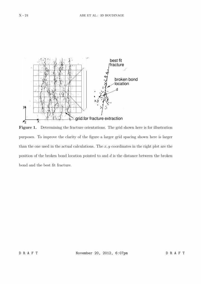
To investigate the orientation of fractures in the boudinaged layer we identify the loca-66

tions of broken bonds in the model. The fracture locations are then projected into the x-y67

(i.e. layer-parallel) plane. The reason why we are restricting the analysis to two dimen-68

sions is that there is little variation in the fracture orientations in the third (z-) dimension.69

An indication of this can be seen in the cross sections in Figure 4 where the fractures are70

oriented mainly parallel to the z-axis. This is also compatible with the expectation that71

the fractures are predominantly tensile and therefore perpendicular to the layering.72

In a next step the model area is decomposed into a square grid (See Fig. 1 - left). A grid73

spacing of 5 model units was chosen, representing about 4% to 5% of the total model size74

in both layer-parallel directions which was either 100 model units for geometry ”A” and75

120 model units for geometry ”B” (see Table 1). For each grid cell a line is determined76

which provides a ”best fit” to the fracture locations (Fig. 1 - right) by minimizing the77

RMS distance between the fracture locations and the line. If there are too few broken78

bonds in a grid section or if the RMS distance between the best fit line and the fracture79

locations is too large, it is assumed that there is no single consistent fracture orientation80

in this particular grid section and no orientation data is recorded. Based on the results of81

a number of tests a threshold of 30 was chosen for the minimum number of broken bonds82

per grid cell. A RMS distance of 1 model unit, i.e. 20% of the grid spacing was used as83



threshold for the fit quality. One of the limitations of this approach is that the algorithm84

will return no orientation data for cases where multiple fractures cross the same grid cell.85

The orientations of the detected fracture segments are then combined into an into angular86

distribution for which the statistical properties can be calculated.87

The outer part of the model space (i.e. outside the grid shown in Fig. 1) is excluded from88

these calculations to avoid boundary e!ects, i.e. fractures always being perpendicular to89

a free surface.90

In order to quantify the anisotropy in the fracture orientation data we tested 3 di!erent91

methods: a Fourier Transform approach, calculating a best fit ellipsis and the ”fabric92

tensor” method. All three methods have their advantages and disadvantages as described93

below, but an evaluation has shown that the ”fabric tensor” method is the most suitable94

one for the purpose of this work.95

A method for the determination of the anisotropy in orientation data suggested in the96

literature (Rothenburg and Bathurst [1989]) is to calculate the Discrete Fourier Transform97

(DFT) of the angular distribution of the orientations, i.e.98

hi =1

N

!

N!1"

i=0

ai cos

#

2!i

N

$

+N!1"

i=0

bi sin

#

2!i

N

$

%

(1)

where hi is the number of fractures which fall in the i-th bin of the orientation his-99

togram and N is the number of histogram bins. Due to the symmetry of the orientation100

distribution only even Fourier-components, i.e. a2i, b2i for i = 0 . . .N/2, are non-zero (see101

Rothenburg and Bathurst [1989]). The values of the ”DC”-component of the DFT, i.e. a0102

in Eq. 1, and the the magnitude of the 2nd Fourier component, i.e.&

a22 + b22 in Eq. 1103

can be used to calculate a measure AF of the anisotropy of the orientation distribution as104



AF =

&

a22 + b22a0

. (2)

Tests with data from some of our models confirmed that the calculated anisotropy105

measure AF is relatively robust with respect to the binning of the orientation histogram.106

Unfortunately, applying this approach to the fracture orientation data obtained from our107

simulations did also show that the fit between the measured data hi and the approximation108

h(") = a0 + a2 cos 2" + b2 sin 2" is not very good, in particular for strongly anisotropic109

distributions (see Fig. 2).110

An alternative would be to calculate a best-fit ellipse and to use the ratio between the111

long axis rl and the short axis rs as a measure for the anisotropy.112

h(") =

'

rs2

1! #2 cos(")2(3)

where # is the numerical eccentricity of the ellipse. The axis ratio can then be calculated113

as114

rlrs

=1

"1! #2

. (4)

While this results in a better fit for some data (see Fig. 2), tests did also show that the115

method has two major drawbacks. Firstly the anisotropy parameters obtained for a given116

orientation distribution show a significant dependence on the bin size of the orientation117

histogram used to calculate the ellipse. Additionally the numerical optimization methods118

employed in the fitting process did not always converge, in particular if the orientation119

distributions were highly anisotropic.120



The ”fabric tensor” has been used used previously to determine the statistical properties121

of the distribution of particle contact directions in granular media ( Madadi et al. [2004];122

Jerier et al. [2008]). We use a similar approach here for the orientation distribution of the123

fractures. The tensor Fij is constructed the same way as described for the fabric tensor124

by Madadi et al. [2004], only that we are using the fracture directions instead of contact125

normals as input data. Therefore the ”orientation fabric tensor” is calculated as126

Fij =1

n

n"

k=1

lki lkj (5)

where n is the number of fractures considered and lki and lkj are the i-th and j-th127

component of the k-th direction vector lk. Here the direction vector is a vector describing128

the orientation of one of the fracture segments found by the algorithm described at the129

beginning of the section (Fig. 1). A measure of the anisotropy of the fracture orientation130

distribution can then be calculated from the ratio of the eigenvalues of the fabric tensor.131

As we are only considering the orientation of the fractures within the layer-parallel plane132

the Fij is a rank-2 tensor and therefore has 2 eigenvalues. Calculating the anisotropy133

coe"cient AT from the eigenvalues as134

AT =e0 ! e1

e0(6)

where e0 is the larger and e1 is the smaller of the two eigenvalues we get AT = 0 for135

the isotropic case and AT = 1 for complete anisotropy, i.e. if all fractures are aligned136

exactly in the same direction. A key advantage of this approach is that it does not involve137

the transformation of the fracture orientation data into a histogram and the results are138

therefore not susceptible to a dependence on the choice of histogram bin size. However,139



unlike the DFT based method described above this approach is not able to detect the140

presence of higher order components in the fracture orientation distribution.141

2.3. Model Setup

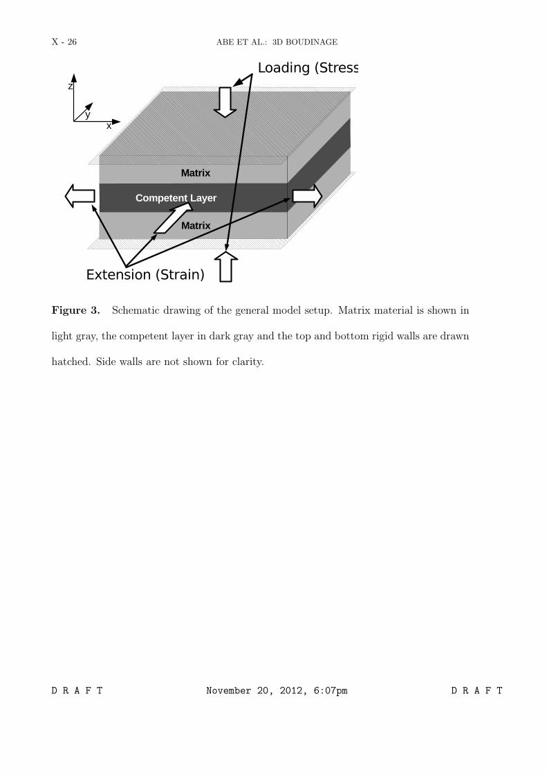
The models consists of a simple 3 layer setup based on the 2D models presented by142

Abe and Urai [2012]. In these models a brittle central layer oriented parallel to the x-y143

plane is embedded between two layers of ductile material. Interactions between particles144

belonging to the central brittle layer and the ductile matrix layers are described by a145

dashpot interaction, i.e. the layer interface is not welded and the drag exerted on the146

central layer by the two ductile layers is dependent on the slip rate at the layer interface.147

All models are square-shaped in the layer-parallel direction, i.e. the model dimensions148

in the x- and y-dimensions are the same. The boundary conditions in all 3 dimensions are149

formed by rigid plates interacting with the DEM particles by elastic forces (Fig. 3). The150

top and bottom plates, i.e. those oriented parallel to the layering are servo-controlled to151

apply a defined normal stress of 0.005 model units to the model. Assuming an Young’s152

modulus E = 20GPa for the material this would be equivalent to a normal stress of153

$n = 10MPa. The four side boundary plates are displacement controlled. During the154

simulations the side boundary plates are initially held stationary while the normal stress155

on the top and bottom is linearly ramped up to the prescribed level. After this the stress156

at top and bottom is held constant and the side boundary plates are moved outwards. The157

velocity of the side plates is also increased linearly until the chosen strain rate is achieved158

and then held constant. This setup allows the precise control of the ratio between the159

layer parallel strain components #xx and #yy during the simulations.160

All models are built using the a similar basic geometry. The model thickness perpen-161



dicular to the layering is 30 model units. The central, competent, layer has a thickness162

of 10 units. The model size in both layer-parallel dimensions is 100 or 120 model units.163

Using a minimum particle radius of 0.2 model units and a maximum particle radius of 1.0164

model units this results in a total of approximately 870.000 particles for the models with165

dimensions 100 # 100 # 30 model units and 1.2 million particles for the 120 # 120 # 30166

models. The exact number varies slightly between the di!erent random realizations of167

the particle packing (Table 1). Given that the ratio between particle radius and layer168

thickness mean that the brittle layer is only $ 10! 20 particles thick, depending on the169

actual particle arrangement, the particles should not be seen as a direct representation of170

rock grains or even crystals but rather as the discretisation of a larger volume of rock.171

Material properties were also adapted from the models by Abe and Urai [2012], i.e. the172

same microscopic interaction properties have been used. The cohesion of the brittle layer173

material is C = 0.0025 model units, making the material properties similar to the interme-174

diate strength models in Abe and Urai [2012]. Typical computing times for these models175

on current computer architectures (Intel Xeon 5675 cluster) are around 500 CPU-hours176

(16-18 hours on 30 cores) for small deformation models used to investigate the fracture177

orientation distribution and 2500 CPU hours for the simulations run to $ 20% extension178

(i.e. Fig. 4).179

3. Results

In order to investigate the influence of the ratio between the extension rates in the two180

layer-parallel directions a series of simulations were performed using strain ratios #xx : #yy181

varying from uniaxial extension in x-direction and isotropic extension. To constrain the182

statistical variability of the results caused by the random particle packing used each183



simulation with a given strain ratio was repeated for 3 realizations of the same basic184

model geometry using a di!erent particle packing. The details of the models are listed in185

Table 2.186

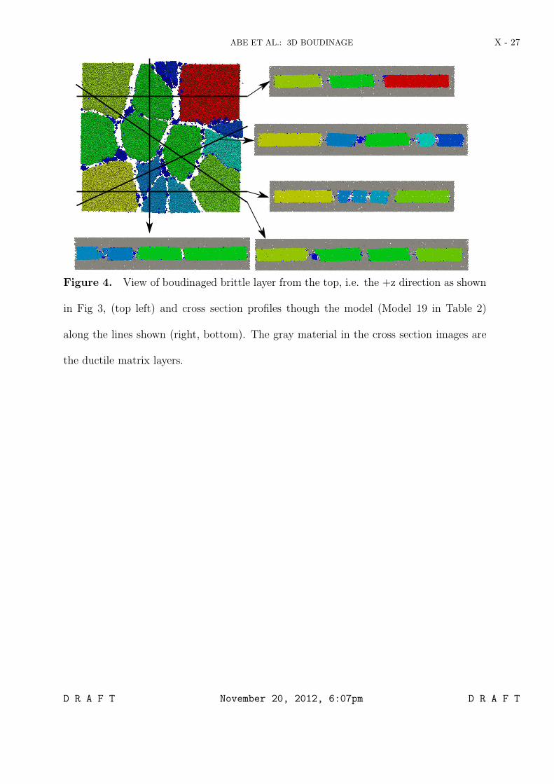
The view of the boudinaged brittle layer parallel to the x-y plane shows either sub-parallel187

or polygonal fracture patterns, depending on the strain conditions (Fig 8, left column).188

Cross section profiles perpendicular to the layering show 2D boudinage structures similar189

to those observed in the pure 2D models by Abe and Urai [2012] (Fig. 4) even in models190

which show a polygonal fracture pattern in 3D. The cross sections suggest that there is191

larger range of apparent boudin block sizes visible in the 2D section through a set of192

polygonal 3D boudins than would be expected from a pure 2D model or a 3D plane strain193

model. This is caused be the possibility that in 3D a cross section is cutting some of the194

boudin blocks near their center so that the apparent block size in the direction along the195

cross section is similar to the true diameter of the block but other blocks are cut closer196

to a corner so that the apparent block length visible in the cross section is much smaller197

than the real diameter of the intersected boudin block. However, due to the limited model198

size there is no quantitative statistical evidence for this observation.199

3.1. Evolution of Fracture Orientations during progressive Deformation

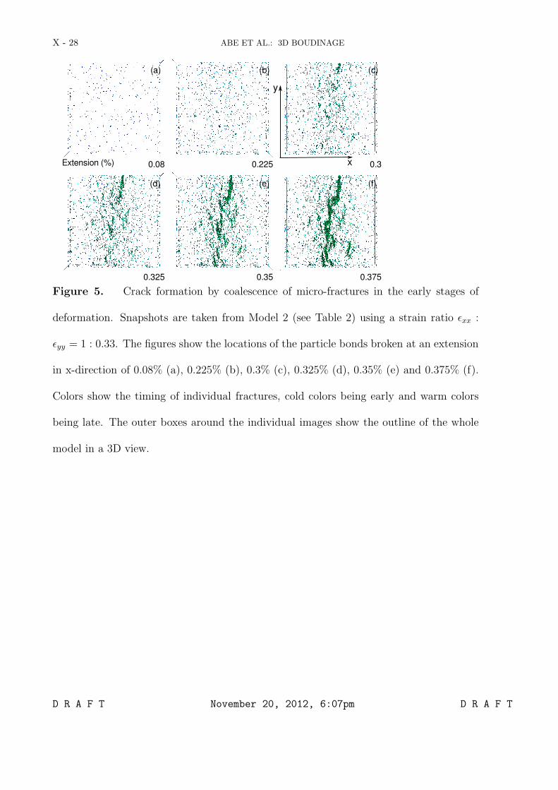
By extracting the time and location when the bonds between particles break it is possi-200

ble to observe in detail how the fracture patterns evolve with increasing strain. The results201

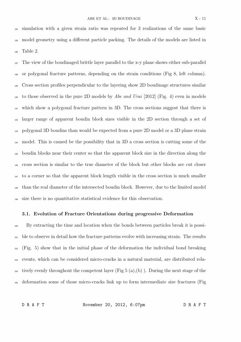
(Fig. 5) show that in the initial phase of the deformation the individual bond breaking202

events, which can be considered micro-cracks in a natural material, are distributed rela-203

tively evenly throughout the competent layer (Fig 5 (a),(b) ). During the next stage of the204

deformation some of those micro-cracks link up to form intermediate size fractures (Fig205



5 (c),(d) ) which finally coalesce into fractures spanning the whole model (Fig 5 (e),(f) ).206

While Figure 5 shows only one example of this process the observations are similar for all207

models investigated in the work. This process shows a strong similarity to observations208

of fracture growth in compression experiments on dolomitic marble by Barnhoorn et al.209

[2010], despite the applied stress and strain conditions being di!erent.210

The fact that the major fractures in the model are generated by the merging of211

intermediate-sized fractures, which in many cases are not perfectly aligned but o!set212

relative to each other, leads to the appearance of steps and relay structures along the213

main fractures. This, together with the mechanical heterogeneity of the model material214

caused by the random particle packing, provides an explanation why we observe mainly215

rough rather than straight fractures in our models.216

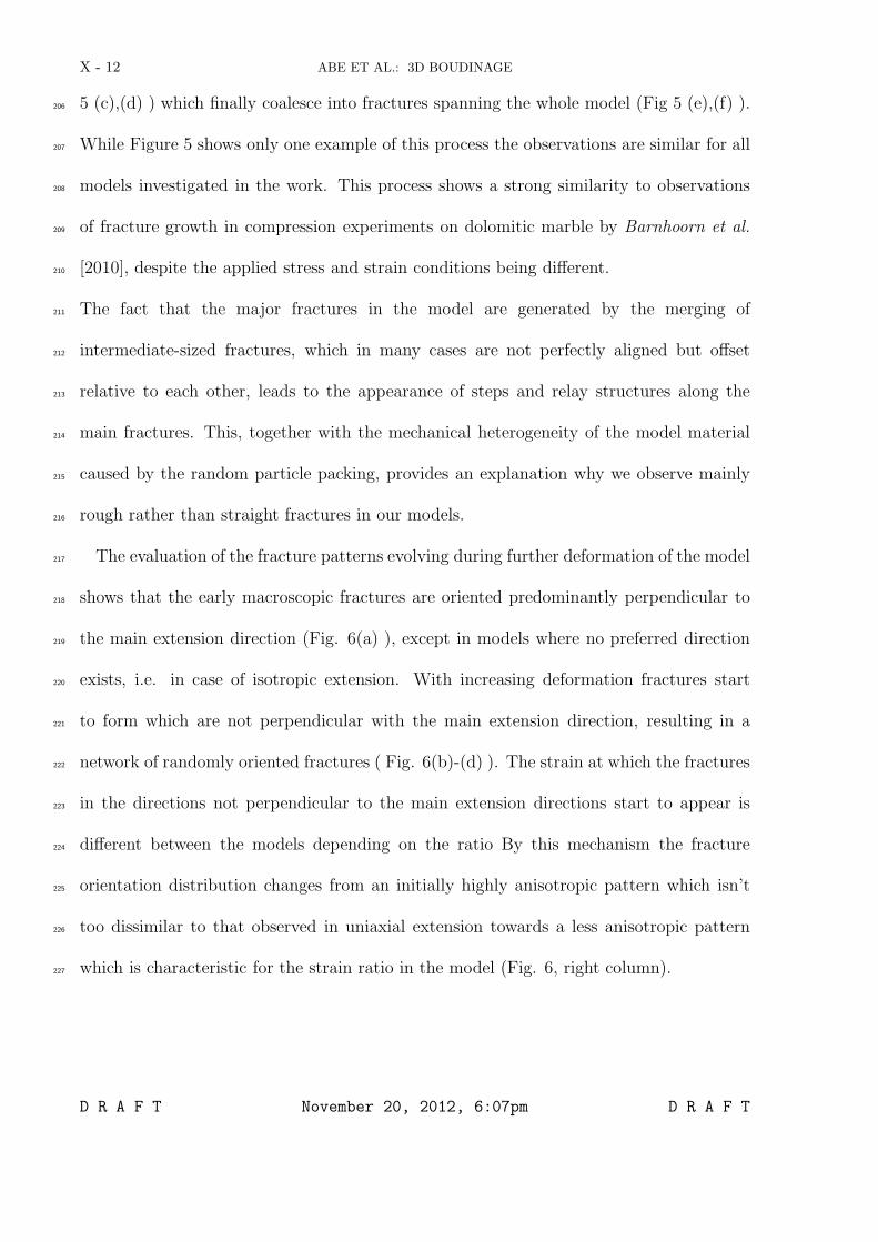
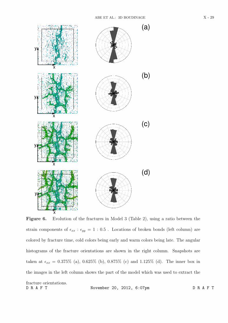
The evaluation of the fracture patterns evolving during further deformation of the model217

shows that the early macroscopic fractures are oriented predominantly perpendicular to218

the main extension direction (Fig. 6(a) ), except in models where no preferred direction219

exists, i.e. in case of isotropic extension. With increasing deformation fractures start220

to form which are not perpendicular with the main extension direction, resulting in a221

network of randomly oriented fractures ( Fig. 6(b)-(d) ). The strain at which the fractures222

in the directions not perpendicular to the main extension directions start to appear is223

di!erent between the models depending on the ratio By this mechanism the fracture224

orientation distribution changes from an initially highly anisotropic pattern which isn’t225

too dissimilar to that observed in uniaxial extension towards a less anisotropic pattern226

which is characteristic for the strain ratio in the model (Fig. 6, right column).227



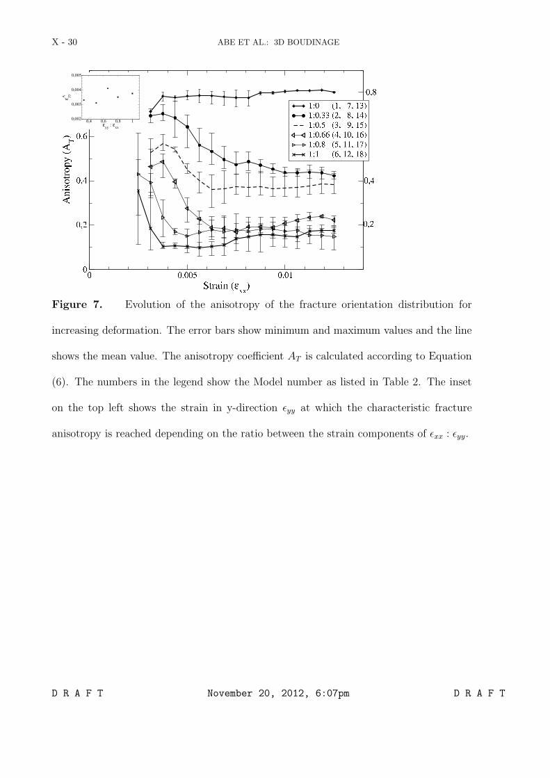
Calculating the degree of anisotropy in the fracture orientation distribution as described228

in section 2.2 during progressive deformation shows that there is a continuous decrease in229

anisotropy towards the final value (Fig. 7). The large scatter of the anisotropy coe"cient230

AT during the early part of the deformation observed in some of the models, in particular231

the models with strain ratios 1:1 and 1:0.8 for strains exx < 0.004, is due to the low232

number of macroscopic fractures at this stage.233

Comparing the evolution of the anisotropy coe"cient AT for the models with di!erent234

strain ratio #xx : #yy in Figure 7 shows that the models with a smaller ratio between the235

strain components reach their characteristic ”steady state” value of the fracture orienta-236

tion anisotropy for less strain in the x-direction than those with a higher strain anisotropy.237

However, the strain in y-direction #yy at which the steady state value of AT is reached238

is much more similar between the models, excluding the model with pure uniaxial ex-239

tension. The strain in y-direction #Ayy at which the characteristic fracture anisotropy is240

reached is approximately #Ayy = #Axx = 0.0037 for the anisotropic model, #Ayy = 0.0035 for241

#xx : #yy = 1 : 0.8, #Ayy = 0.0041 for #xx : #yy = 1 : 0.66, #Ayy = 0.0031 for #xx : #yy = 1 : 0.5242

and #Ayy = 0.0033 for #xx : #yy = 1 : 0.33 (top left inset in Figure 7). These values suggest243

that the characteristic fracture anisotropy is reached when the extension in the direction244

with lower strain rate, i.e. in y-direction in this case, exceeds a critical value.245

3.2. Fracture Orientations vs. Strain Ratio

The investigation of the fracture evolution in section 3.1 did show that the characteristic246

fracture patterns stabilize at relatively small layer-parallel strains of #xx % 1% (see Fig. 7).247

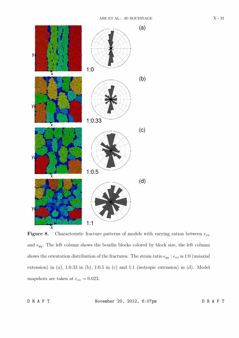
The final fracture patterns observed in the models are dependent on the ratio between the248

two layer-parallel strain components #xx : #yy (Fig. 8). We observe sub-parallel alignment249



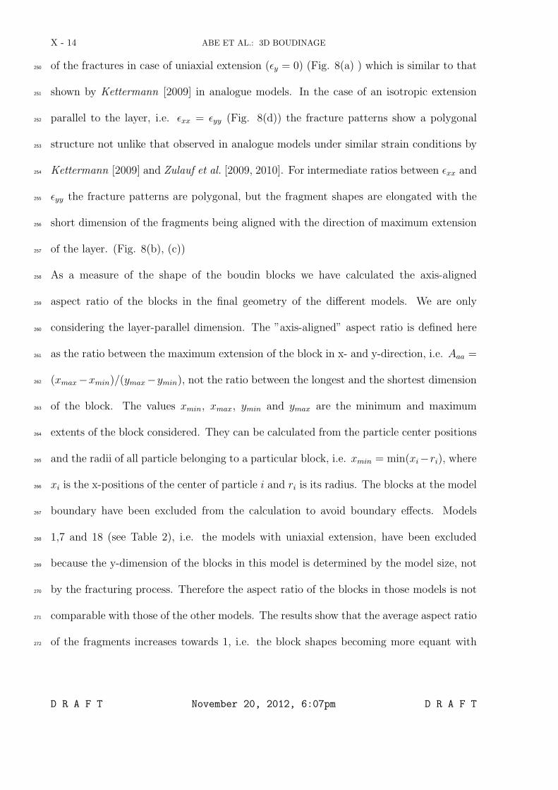
of the fractures in case of uniaxial extension (#y = 0) (Fig. 8(a) ) which is similar to that250

shown by Kettermann [2009] in analogue models. In the case of an isotropic extension251

parallel to the layer, i.e. #xx = #yy (Fig. 8(d)) the fracture patterns show a polygonal252

structure not unlike that observed in analogue models under similar strain conditions by253

Kettermann [2009] and Zulauf et al. [2009, 2010]. For intermediate ratios between #xx and254

#yy the fracture patterns are polygonal, but the fragment shapes are elongated with the255

short dimension of the fragments being aligned with the direction of maximum extension256

of the layer. (Fig. 8(b), (c))257

As a measure of the shape of the boudin blocks we have calculated the axis-aligned258

aspect ratio of the blocks in the final geometry of the di!erent models. We are only259

considering the layer-parallel dimension. The ”axis-aligned” aspect ratio is defined here260

as the ratio between the maximum extension of the block in x- and y-direction, i.e. Aaa =261

(xmax!xmin)/(ymax!ymin), not the ratio between the longest and the shortest dimension262

of the block. The values xmin, xmax, ymin and ymax are the minimum and maximum263

extents of the block considered. They can be calculated from the particle center positions264

and the radii of all particle belonging to a particular block, i.e. xmin = min(xi!ri), where265

xi is the x-positions of the center of particle i and ri is its radius. The blocks at the model266

boundary have been excluded from the calculation to avoid boundary e!ects. Models267

1,7 and 18 (see Table 2), i.e. the models with uniaxial extension, have been excluded268

because the y-dimension of the blocks in this model is determined by the model size, not269

by the fracturing process. Therefore the aspect ratio of the blocks in those models is not270

comparable with those of the other models. The results show that the average aspect ratio271

of the fragments increases towards 1, i.e. the block shapes becoming more equant with272



the strain ratio getting closer to 1, i.e. the strain rates in x- and y-direction becoming273

more similar (Fig. 9). However, this connection becomes weak for models approaching274

isotropic layer-parallel extension (#yy/#xx & 0.8).275

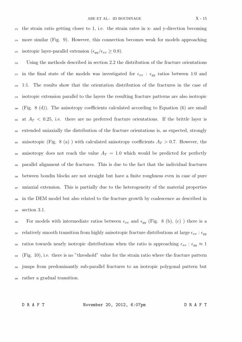
Using the methods described in section 2.2 the distribution of the fracture orientations276

in the final state of the models was investigated for #xx : #yy ratios between 1:0 and277

1:1. The results show that the orientation distribution of the fractures in the case of278

isotropic extension parallel to the layers the resulting fracture patterns are also isotropic279

(Fig. 8 (d)). The anisotropy coe"cients calculated according to Equation (6) are small280

at AT < 0.25, i.e. there are no preferred fracture orientations. If the brittle layer is281

extended uniaxially the distribution of the fracture orientations is, as expected, strongly282

anisotropic (Fig. 8 (a) ) with calculated anisotropy coe"cients AT > 0.7. However, the283

anisotropy does not reach the value AT = 1.0 which would be predicted for perfectly284

parallel alignment of the fractures. This is due to the fact that the individual fractures285

between boudin blocks are not straight but have a finite roughness even in case of pure286

uniaxial extension. This is partially due to the heterogeneity of the material properties287

in the DEM model but also related to the fracture growth by coalescence as described in288

section 3.1.289

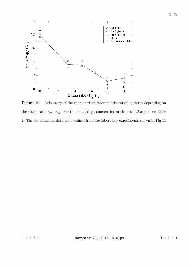
For models with intermediate ratios between #xx and #yy (Fig. 8 (b), (c) ) there is a290

relatively smooth transition from highly anisotropic fracture distributions at large #xx : #yy291

ratios towards nearly isotropic distributions when the ratio is approaching #xx : #yy $ 1292

(Fig. 10), i.e. there is no ”threshold” value for the strain ratio where the fracture pattern293

jumps from predominantly sub-parallel fractures to an isotropic polygonal pattern but294

rather a gradual transition.295



4. Discussion

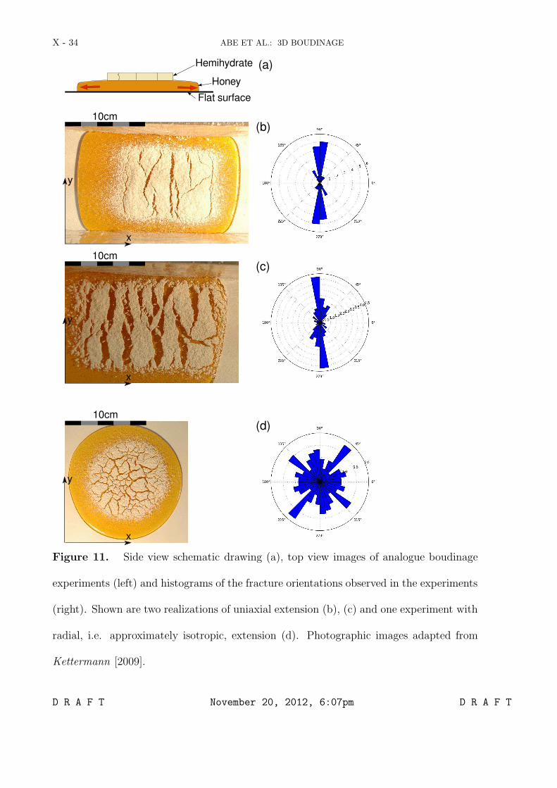
The fracture orientation distributions for the end member models, i.e. uni-axial exten-296

sion and layer-parallel isotropic extension are similar to those observed in the equivalent297

analogue experiments by Kettermann [2009]. These models consisted of a layer of brittle-298

cohesive material (hemihydrate powder) on top of a single layer of a viscous material299

(honey) (Fig 11 (a)). During gravitational spreading of the viscous layer a tensile stress300

is exerted on the brittle hemihydrate layer causing it to fracture. Despite the di!erent301

boundary conditions, the fracture patterns (Fig. 11, left) appear visually not too di!erent302

from those generated in the numerical models (Fig. 8, right ). The fracture orientation303

histograms as shown in the right part of Figure 11 for the experiment and the right col-304

umn of Figure 8 for the numerical models are also similar. Specifically results of the305

experiments under uniaxial extension (Fig. 11 (b) and (c)) show similar fracture patterns306

to the numerical models under uniaxial extension (Fig. 8 (a)) and the fracture patterns307

in the experiment and the numerical models with isotropic extension (Fig. 11 (d), Fig.308

8 (d)) are similar. The calculated anisotropy coe"cients are also comparable. The value309

for the isotropic extension experiment is AT = 0.033 while the value for the equivalent310

numerical models is AT = 0.10 ! 0.23. For the case of uniaxial extension the values are311

AT = 0.70 and AT = 0.88 for the experiments and AT = 0.76 ! 0.80 for the numerical312

models.313

One feature of the numerical boudin models is that, as shown in Figure 8 (a), the fractures314

between the boudin blocks are rough rather than straight even in case of pure uniaxial ex-315

tension. Due to the limited amount of information available about the three-dimensional316

geometry of natural boudins it is not clear how common this feature is in nature. However,317



observations in analogue models suggest that the fractures between the boudin blocks are318

rough rather than straight in those experiments. See for example the models by Ketter-319

mann [2009] and Figure 3 in Kidan and Cosgrove [1996].320

These results might point towards a possibility to use the connection between the de-321

gree of anisotropy and the strain ratio as tool to constrain the deformation history of322

real 3D boudins. Such a tool would be particularly useful in situations where the flow of323

the matrix material is complicated and spatially heterogeneous such as the 100m-km scale324

boudinage of carbonate and anhydrite layers embedded in deformed salt bodies (van Gent325

et al. [2011]; Strozyk et al. [2012]). However, further work will be needed to confirm the326

observed connection for real boudins. In particular a comparison of the simulation results327

with data obtained from analogue models or possibly field data would be useful. Such328

comparisons would provide additional information to what extent the simplified material329

properties used in the DEM model are influencing the patterns formed in a boudinage330

process, for example with respect to the fact the the competent layer in the models used331

here is completely brittle whereas some natural materials show ductile creep in addition332

to brittle failure.333

The polygonal fracture patterns for isotropic layer parallel extension (pure flattening)334

and for models with intermediate strain ratios are always composed of random unevenly335

shaped polygons in our models which is consistent with observations from analogue models336

using similar strain conditions (Kettermann [2009]; Zulauf et al. [2009, 2010]) . We do not337

observe a classic ”chocolate tablet” boudinage dominated by two dominant perpendicular338

fracture directions as described by Ghosh [1988] and Zulauf et al. [2011b].339



5. Conclusions

The results of the study confirm that the Discrete Element Method (DEM) is a suit-340

able tool for the numerical modeling of boudinage processes in 3D. The comparison with341

the work of Kettermann [2009] shows that the models closely reproduce the boudinage342

patterns obtained in analogue models. While the computational costs are relatively high343

and the resolution of the models still remains below that of 2D models the works show344

that 3D models are viable and do provide additional insights which could not be obtained345

from 2D models alone.346

The two key results from the 3D DEM modeling of boudinage are that (a) there is a clear347

connection between the strain ratio in the two layer-parallel dimensions and the anisotropy348

of the resulting fracture pattern and (b) the degree of fracture orientation anisotropy does349

evolve during increasing deformation until it reaches a value characteristic for a particular350

#xx : #yy strain ratio.351

Acknowledgments.352

This study was carried out within the framework of DGMK (German Society for353

Petroleum and Coal Science and Technology) research project 718 ”Mineral Vein Dynam-354

ics Modelling”, which is funded by the companies ExxonMobil Production Deutschland355

GmbH, GDF SUEZ E&P Deutschland GmbH, RWE Dea AG and Wintershall Holding356

GmbH, within the basic research programme of the WEG Wirtschaftsverband Erdol- und357

Erdgasgewinnung e.V. We thank the companies for their finacial support and their per-358

mission to publish these results.359

The main computations for this work were performed using the HPC cluster at RWTH360

Aachen University.361



We also thank the reviewers Elizabeth Ritz and Auke Barnhoorn and editor Tom Parsons362

for their helpful contributions.363

References

Abe, S., and J. L. Urai (2012), Discrete element modeling of boudinage: Insights on364

rock rheology, matrix flow and evolution of geometry., J. Geophys. Res., 117, doi:365

10.1029/2011JB008555.366

Abe, S., D. Place, and P. Mora (2003), A parallel implementation of the lattice solid model367

for the simulation of rock mechanics and earthquake dynamics, Pure. Appl. Geophys.,368

161.369

Bai, T., and D. D. Pollard (1999), Spacing of fractures in a multilayer at fracture satura-370

tion, International Journal of Fracture, 100, L23–L28.371

Bai, T., D. Pollard, and H. Gao (2000), Explanation for fracture spacing in layered ma-372

terials, Nature, 403, 753–755.373

Barnhoorn, A., S. F. Fox, D. J. Robinson, and T. Senden (2010), Stress- and fluid-driven374

failure during fracture array growth: Implications for coupled defornation and fluid flow375

in the crust, Geology, doi:10.1130/G31010.1.376

Cundall, P. A., and O. Strack (1979), A discrete numerical model for granular assemblies,377

Geotechnique, 29, 47–65.378

Ghosh, S. (1988), Theory of chocolate tablet boudinage, Journal of Structural Geology,379

10 (6), 541 – 553, doi:10.1016/0191-8141(88)90022-3.380

Goscombe, B., and C. Passchier (2003), Asymmetric boudins as shear sense indicators -381

an assessment from field data, J. Struct. Geol., 25 (4), 575–589.382



Goscombe, B. D., C. W. Passchier, and M. Hand (2004), Boudinage classification: end-383

member boudin types and modified boudin structures, J. Struct. Geol., 26 (4), 739–763.384

Iyer, K., and Y. Y. Podladchikov (2009), Transformation-induced jointing as a gouge for385

interfacial slip and rock strength, Earth Planet. Sci. Lett., 280, 159–166.386

Jerier, J.-F., D. Imbault, F. Donze, and R. Doremus (2008), A geometric algorithm based387

on tetrahedral meshes to generate a dense polydisperse sphere packing, Granular Matter.388

Kettermann, M. (2009), The analogue modeling of boudins., BSc-Thesis, RWTH Aachen389

University.390

Kidan, T., and J. Cosgrove (1996), The deformation of multilayers by layer-normal an391

experimental investigation, J. Struct. Geol., 18 (4), 461–474.392

Li, Y., and C. Yang (2007), On fracture saturation in layered rocks, Int. J. Rock Mech.393

and Min. Sci., 44, 936–941.394

Madadi, M., O. Tsoungui, M. Ltzel, and S. Luding (2004), On the fabric tensor of poly-395

disperse granular materials in 2d, Int. J. Solid. Struct., 41, 2563–2580.396

Maeder, X., C. W. Passchier, and D. Koehn (2009), Modelling of segment structures:397

Boudins, bone-boudins, mullions and related single- and multiphase deformation fea-398

tures, J. Struct. Geol., 31 (8), 817–830.399

Mandal, N., and D. Khan (1991), Rotation, o!set and separation of oblique-fracture400

(rhombic) boudins - theory and experiements under layer-normal compression, J. Struct.401

Geol., 13 (3), 349–356.402

Mandal, N., C. Chakraborty, and S. K. Samanta (2000), Boudinage in multi-layered rocks403

under layer-normal compression - a theoretical analysis, J. Struct. Geol., 22, 373–382.404



Middleton, G. V., and P. R. Wilcock (1994), Mechanics in the Earth and Environmental405

Sciences, Cambridge University Press.406

Mora, P., and D. Place (1994), Simulation of the frictional stick-slip instability, Pure Appl.407

Geophys., 143, 61–87.408

Passchier, C. W., and E. Druguet (2002), Numerical modelling of asymmetric boudinage,409

J. Struct. Geol., 24, 1789–1803.410

Place, D., and P. Mora (1999), The lattice solid model: incorporation of intrinsic friction,411

J. Int. Comp. Phys., 150, 332–372.412

Potyondy, D., and P. Cundall (2004), A bonded-particle model for rock, Int. J. Rock413

Mech. and Min. Sci., 41 (8), 1329–1364.414

Ramberg, H. (1955), Natural and experimental boudinage and pinch-and-swell structures,415

Journal of Geology, 63, 512–526.416

Ramsay, J. G., and M. I. Huber (1987), The Techniques of Modern Structural Geology,417

Academic Press.418

Rothenburg, L., and R. Bathurst (1989), Analytical study of induced anisotropy in ideal-419

ized granular materials, Geotechnique, 39 (4), 601–614.420

Schenk, O., J. L. Urai, and W. van der Zee (2007), Evolution of boudins under progres-421

sively decreasing pore pressure - a case study of pegmatites enclosed in marble deforning422

at high grade metamorphic conditions, naxos, greece, American Journal of Science, 307,423

1009–1033, doi:10.2475/07.2007.03.424

Strozyk, F., H. van Gent, J. Urai, and P. A. Kukla (2012), 3d seismic study of complex425

intra-salt deformation: an example from the upper Permian Zechstein 3 stringer, west-426

ern Dutch o!shore, in Salt tectonics, Sediments and Prospectivity, Special Publications,427



vol. 363, edited by G. Alsop, S. Archer, A. Hartley, N. Grant, and R. Hodgkinson, pp.428

489–501, Geological Society of London, doi:10.1144/SP363.23.429

Twiss, R. J., and E. M. Moores (2007), Structural Geology, second ed., W. H. Freeman430

and Company.431

van Gent, H., J. L. Urai, and M. de Keijzer (2011), The internal geometry of salt structures432

- a first look using 3d seismic data from the zechstein of the netherlands, J. Struct. Geol.,433

33, 292–311.434

Wang, Y., S. Abe, S. Latham, and P. Mora (2006), Implementation of particle-scale435

rotation in the 3-d lattice solid model, Pure Appl. Geophys., 163, 1769–1785.436

Weatherley, D., V. Boros, W. Hancock, and S. Abe (2010), Scaling benchmark of esys-437

particle for elastic wave propagation simulations, in Sixth IEEE International Confer-438

ence on eScience, Brisbane, Australia.439

Zulauf, G., J. Zulauf, O. Bornemann, N. Kihm, M. Peinl, and F. Zanella (2009), Ex-440

perimental deformation of a single-layer anhydrite in halite matrix under bulk con-441

striction. part 1: Geometric and kinematic aspects, J. Struct. Geol., 31, 460–474, doi:442

10.1016/j.jsg.2009.01.013.443

Zulauf, G., J. Zulauf, O. Bornemann, F. Brenker, H. Hofer, M. Peinl, and A. Woodland444

(2010), Experimental deformation of a single-layer anhydrite in halite matrix under bulk445

constriction. part 2: Deformation mechanisms and the role of fluids, J. Struct. Geol.,446

32 (3), 264–277, doi:10.1016/j.jsg.2009.12.001.447

Zulauf, G., G. Gutierrez-Alonso, R. Kraus, R. Petschick, and S. Potel (2011a), Formation448

of chocolate-tablet boudins in a foreland fold and thrust belt: A case study from the449

external Variscides (Almograve, Portugal), J. Struct. Geol., 33 (11), 1639–1649, doi:450



10.1016/j.jsg.2011.08.009.451

Zulauf, J., G. Zulauf, R. Kraus, G. Gutierrez-Alonso, and F. Zanella (2011b), The origin452

of tablet boudinage: Results from experiments using power-law rock analogs, Tectono-453

physics, 510 (3-4), 327–336, doi:10.1016/j.tecto.2011.07.013.454



best fit fracture

x,y

d

broken bondlocation

x

y

zgrid for fracture extraction

Figure 1. Determining the fracture orientations. The grid shown here is for illustration

purposes. To improve the clarity of the figure a larger grid spacing shown here is larger

than the one used in the actual calculations. The x, y coordinates in the right plot are the

position of the broken bond location pointed to and d is the distance between the broken

bond and the best fit fracture.



0°

45°

90°

135°

180°

225°

270°

315°

0.51.0

1.52.0

2.53.0

Figure 2. Histogram of orientation distribution (blue), best-fit approximations based

on the first two Fourier components (red) and best-fit ellipse (black). The positive x-axis

is oriented towards 0 degrees and the positive y-axis towards 90 degrees.



Figure 3. Schematic drawing of the general model setup. Matrix material is shown in

light gray, the competent layer in dark gray and the top and bottom rigid walls are drawn

hatched. Side walls are not shown for clarity.



Figure 4. View of boudinaged brittle layer from the top, i.e. the +z direction as shown

in Fig 3, (top left) and cross section profiles though the model (Model 19 in Table 2)

along the lines shown (right, bottom). The gray material in the cross section images are

the ductile matrix layers.



(a) (b) (c)

(d) (e) (f)

Extension (%) 0.08 0.225 0.3

0.325 0.35 0.375

x

y

Figure 5. Crack formation by coalescence of micro-fractures in the early stages of

deformation. Snapshots are taken from Model 2 (see Table 2) using a strain ratio #xx :

#yy = 1 : 0.33. The figures show the locations of the particle bonds broken at an extension

in x-direction of 0.08% (a), 0.225% (b), 0.3% (c), 0.325% (d), 0.35% (e) and 0.375% (f).

Colors show the timing of individual fractures, cold colors being early and warm colors

being late. The outer boxes around the individual images show the outline of the whole

model in a 3D view.



(a)

(b)

(c)

(d)

x

y

x

y

x

y

x

y

Figure 6. Evolution of the fractures in Model 3 (Table 2), using a ratio between the

strain components of #xx : #yy = 1 : 0.5 . Locations of broken bonds (left column) are

colored by fracture time, cold colors being early and warm colors being late. The angular

histograms of the fracture orientations are shown in the right column. Snapshots are

taken at #xx = 0.375% (a), 0.625% (b), 0.875% (c) and 1.125% (d). The inner box in

the images in the left column shows the part of the model which was used to extract the

fracture orientations.D R A F T November 20, 2012, 6:07pm D R A F T


0,4 0,6 0,8 1εyy : εxx

0,002

0,003

0,004

0,005

εA yy

Figure 7. Evolution of the anisotropy of the fracture orientation distribution for

increasing deformation. The error bars show minimum and maximum values and the line

shows the mean value. The anisotropy coe"cient AT is calculated according to Equation

(6). The numbers in the legend show the Model number as listed in Table 2. The inset

on the top left shows the strain in y-direction #yy at which the characteristic fracture

anisotropy is reached depending on the ratio between the strain components of #xx : #yy.



(a)

(b)

(c)

(d)

1:0

1:0.33

1:0.5

1:1

x

y

x

y

x

y

x

y

Figure 8. Characteristic fracture patterns of models with varying ration between #xx

and #yy. The left column shows the boudin blocks colored by block size, the left column

shows the orientation distribution of the fractures. The strain ratio #yy : #xx is 1:0 (uniaxial

extension) in (a), 1:0.33 in (b), 1:0,5 in (c) and 1:1 (isotropic extension) in (d). Model

snapshots are taken at #xx = 0.023.



Figure 9. Average aspect ratio of the boudin blocks in models with varying ration

between #xx and #yy. Aspect ratio is calculated as (xmax ! xmin)/(ymax ! ymin) for each

boudin block. Model snapshots are taken at #xx = 0.023. For the detailed parameters for

model sets 1,2 and 3 see Table 2.



Figure 10. Anisotropy of the characteristic fracture orientation patterns depending on

the strain ratio #xx : #yy. For the detailed parameters for model sets 1,2 and 3 see Table

2. The experimental data are obtained from the laboratory experiments shown in Fig 11



(b)

(c)

(d)10cm

10cm

10cm

Hemihydrate

Honey

Flat surface

(a)

x

y

x

y

x

y

Figure 11. Side view schematic drawing (a), top view images of analogue boudinage

experiments (left) and histograms of the fracture orientations observed in the experiments

(right). Shown are two realizations of uniaxial extension (b), (c) and one experiment with

radial, i.e. approximately isotropic, extension (d). Photographic images adapted from

Kettermann [2009].



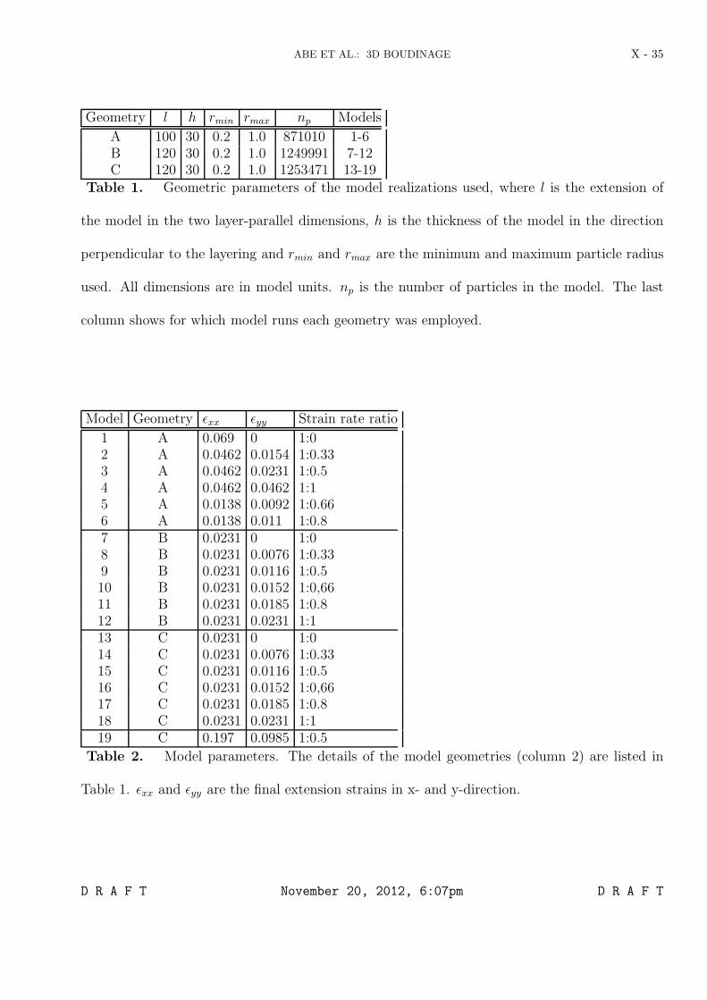
Geometry l h rmin rmax np Models

A 100 30 0.2 1.0 871010 1-6B 120 30 0.2 1.0 1249991 7-12C 120 30 0.2 1.0 1253471 13-19

Table 1. Geometric parameters of the model realizations used, where l is the extension of

the model in the two layer-parallel dimensions, h is the thickness of the model in the direction

perpendicular to the layering and rmin and rmax are the minimum and maximum particle radius

used. All dimensions are in model units. np is the number of particles in the model. The last

column shows for which model runs each geometry was employed.

Model Geometry #xx #yy Strain rate ratio

1 A 0.069 0 1:02 A 0.0462 0.0154 1:0.333 A 0.0462 0.0231 1:0.54 A 0.0462 0.0462 1:15 A 0.0138 0.0092 1:0.666 A 0.0138 0.011 1:0.87 B 0.0231 0 1:08 B 0.0231 0.0076 1:0.339 B 0.0231 0.0116 1:0.510 B 0.0231 0.0152 1:0,6611 B 0.0231 0.0185 1:0.812 B 0.0231 0.0231 1:113 C 0.0231 0 1:014 C 0.0231 0.0076 1:0.3315 C 0.0231 0.0116 1:0.516 C 0.0231 0.0152 1:0,6617 C 0.0231 0.0185 1:0.818 C 0.0231 0.0231 1:119 C 0.197 0.0985 1:0.5

Table 2. Model parameters. The details of the model geometries (column 2) are listed in

Table 1. #xx and #yy are the final extension strains in x- and y-direction.


fracture patterns in non-plane strain boudinage · 2013-02-18 · 1 fracture patterns in non-plane...

Documents