Free LSD: Prior-Free Visual Landing Site Detectionfor Autonomous Planes

Timo Hinzmann, Thomas Stastny, Cesar Cadena, Roland Siegwart, and Igor Gilitschenski

Abstract— Full autonomy for fixed-wing unmanned aerialvehicles (UAVs) requires the capability to autonomously detectpotential landing sites in unknown and unstructured terrain,allowing for self-governed mission completion or handling ofemergency situations. In this work, we propose a perceptionsystem addressing this challenge by detecting landing sitesbased on their texture and geometric shape without usingany prior knowledge about the environment. The proposedmethod considers hazards within the landing region suchas terrain roughness and slope, surrounding obstacles thatobscure the landing approach path, and the local wind fieldthat is estimated by the on-board EKF. The latter enablesapplicability of the proposed method on small-scale autonomousplanes without landing gear. A safe approach path is computedbased on the UAV dynamics, expected state estimation andactuator uncertainty, and the on-board computed elevationmap. The proposed framework has been successfully tested onphoto-realistic synthetic datasets and in challenging real-worldenvironments.

I. INTRODUCTION

Small-scale autonomous planes promise to become aubiquitous tool in the commercial, industrial, and scientificsectors due to reduced operational costs and ever increasingrobustness. Especially the ability to map large areas andto carry out perpetual surveillance tasks, e.g. by using asolar-powered platform, makes this type of unmanned aerialvehicles (UAVs) interesting for various applications. Whilemission operation can already be completely automated [1],appropriate landing site detection (LSD) and the actuallanding procedure still requires an experienced safety pilot.Furthermore, in future fully autonomous beyond visual line-of-sight (BVLOS) operation, finding an appropriate landingspot in unstructured terrain is essential for handling emer-gency scenarios.

Existing LSD systems focus on the cases of vertical takeoffand landing (VTOL) platforms, or large-scale planes, mayrely on offline-computed data, or require prior knowledgeabout the environment. These approaches are not suitedfor small-scale autonomous planes operating in unknownenvironments which are constrained by potentially limitedenergy supply and computational power. Furthermore, theirsize and speed requires taking the wind into consideration,and due to their potential absence of landing gear, preferablylanding in flat grass to not damage wings or fuselage.

The present work proposes Free LSD, a real-time vi-sual landing site detection and approach path computationalgorithm for autonomous fixed-wing UAVs. To keep the

1 All authors are with the Swiss Federal Institute of Technology (ETH)Zurich, Autonomous Systems Lab (www.asl.ethz.ch), Leonhardstrasse 21,CH-8092 Zurich, Switzerland. {firstname.lastname}@mavt.ethz.ch.

Fig. 1: The goal is to find the optimal landing spot while con-sidering terrain shape, terrain texture, terrain roughness, terrainslope, surrounding obstacles, estimated local wind field, and UAVdynamics and their uncertainties.

problem complexity manageable, potential landing sites aretracked and ranked over multiple frames. Only the mostpromising landing sites are forwarded for finer grained, 3 Dprocessing. No a priori data such as markers, pre-classifiedDigital Surface Maps (DSM), or orthomosaics are utilizedwhich allows the framework to be operated in completelyunknown terrain as is exemplary shown in Fig. 1. To the bestof the authors’ knowledge, this paper presents the first suchsystem, which is also suitable for application on small-scaleUAVs. The work incorporates wind field and nearby obstacleconsideration during approach path generation and decisionmaking. Performance of the full framework is evaluated inunknown terrain using various synthetic datasets and real-world test flights.

II. RELATED WORK

Automated landing of VTOL UAVs has been consid-ered in a broad body of works. For instance, Desarajuet al. [2] propose a vision-based landing site evaluationframework to land on rooftops employing a Gaussian processto estimate the landing site confidence. Forster et al. [3]present an efficient way to compute a vision-based elevationmap on-board of a quadrocopter. Johnson et al. [4] use aLIDAR-based elevation map to compute terrain smoothness,roughness, and incidence angles to determine safe landingspots for spacecrafts. Garcia-Padro et al. [5] introduce acontrast descriptor to land an autonomous helicopter far awayfrom obstacles under the assumption that the terrain is flat.

Brockers [6], Cheng [7], and Bosch et al. [8] make use ofhomography decomposition for identifying planar landingspots. Theodore et al. [9] employ a stereo vision rig mountedon an unmanned helicopter to compute a range map and infersafe landing spots based on roughness, slope and distanceto closest obstacle. The above approaches have in commonthat the main criterion for VTOL UAVs is flatness of thelanding spot. However, our application requires taking theplane dynamics and additional space requirements duringlanding into consideration.

For fixed-wing platforms, most research focuses on caseswhere the system recognizes modified environments or man-made structures, or where the landing site is pre-defined.Visual servoing is employed by Huh et al. [10] to steer asmall fixed-wing UAS into a red dome-shaped airbag locatedin an obstacle-free area. Similarly, the framework proposedby Laiacker et al. [11] recognises a runway from the UAVand compares it to a known model. Given a designated,obstacle-free landing site, the height above the ground planecan be estimated using monocular visual-inertial [12] orbiologically inspired stereo vision [13].

In contrast to the aforementioned works, this paper aimsat actively selecting appropriate landing spots in an unknownenvironment. This requires generation and assessment ofpotential candidate areas which has, to the best of our knowl-edge, only been discussed in two publications. Fitzgeraldet al. [14] seek to find suitable areas for crash-landing anairplane in case of emergency. This is achieved by detectingareas without edges on a low-quality image from a definedheight of 2500 ft, before classifying them in order to retrievelarge grass fields. However, relying on a fixed height makesthis approach disadvantageous in case of emergencies. Theclosest approach to ours is presented by Warren et al. [15].However, we see the following caveats that we address withthe present work. Firstly, the terrain classification is derivedfrom stored data.Secondly, the approach trajectory and heightof nearby obstacles is only considered indirectly by thePrincipal Component Analysis (PCA). Thirdly, wind is notconsidered which has a large effect on smaller and light-weight planes. Finally, the approach by Warren et al. [15]does not run in real-time.

III. THE APPROACH

An overview of our proposed algorithm for the detection oflanding sites is shown in Fig. 2: The raw image is segmentedinto homogeneous regions (Sec. III-C) and classified intograss or ¬grass using a binary Random Forest (RF)classifier (Sec. III-D). In parallel, the on-board EKF of thePixhawk autopilot estimates UAV pose and local wind field(Sec. III-A), and depending on the provided image rateand overlap of subsequent frames, a tracker or matcher isemployed to connect consecutive camera frames via featuretracks. Resulting coarse depth measurements (Sec. III-B)are used in the region manager to track region of interests(ROI) based on geometry. The region manager (Sec. III-E)accumulates all information about the regions and ensuresconsistency and uniqueness by merging regions. Based on

these metrics, a coarse grade determines which region ispassed on as a candidate to the fine, 3D evaluation backend.The fine evaluation backend is periodically updated by thefrontend with the n most promising ROIs. All observationsof a ROI, UAV pose estimates, and previously generatedfeature tracks are used to perform key-frame based bundleadjustment (BA) and dense 3D reconstruction (Sec. III-F).Metrics such as terrain slope and roughness (Sec. III-G)are derived from the classification results and 3D model.A distance-to-hazard map determines the landing spot withmaximum distance to the next hazard. Based on this touchdown point, the estimated local wind field (Sec. III-H, III-I),and the 2.5D elevation map, a collision-free approach pathis computed. The final decision module outputs the landingsite location, optimal approach vector, and statistics about thefinal landing site. The actual tracking of the final approachpath is described in [1]. The metrics of the best landingsites are stored to be able to land quickly in the case of anemergency.

A. State Estimation

The state estimator on the Pixhawk autopilot estimatesbody poses, velocities, IMU biases, and the wind fieldusing GNSS, IMU, magnetometer, and pressure measure-ments [16]. The camera pose estimates are forwarded tothe on-board computer which associates camera poses to thecorresponding images based on the pre-calibrated camera-IMU transformation [17]. These camera pose estimates areused as priors in the bundle adjustment if an area was markedas potential landing spot. Additionally, feature tracks aregenerated using, depending on the provided framerate, aKanade-Lucas-Tomasi (KLT) [18] feature tracker or matcher.These feature tracks are used to generate coarse depthmeasurements (cf. Sec. III-B for region tracking in unknownterrain and in the bundle adjustment of the backend thread(cf. Sec. III-F).

B. Coarse Depth Measurements

To obtain a segmentation that is robust to height changesas well as for geometric region tracking, coarse depthmeasurements are required in the frontend (cf. Sec. III-E). Since our system is designed to operate in unknownterrain without a priori data, the depth measurements needto be retrieved at runtime1. One possibility would be totriangulate a few features at every step and build up amesh by using, for instance, Delaunay triangulation [19].However, to obtain depth measurements at a given pixel,computationally expensive ray-casting queries would be re-quired. Furthermore, a depth image obtained from two viewsfrom a virtual stereo rig based on unoptimized camera poseestimates is prone to errors since we assume a noisy low-level state estimator. Instead, we take advantage of the featuretracking thread that is running in parallel: To map from2D to 3D coordinates, the N feature tracks closest to thequeried keypoint location are determined. The final height

1Depending on the application and flight altitude, the coarse depthmeasurements could be obtained from a ground plane approximation.

- Region tracker- Region merger- Grade regions (area, classif.)- Associate images & regions

Binary Random ForestCanny Edge Detector,Distance TransformCamera

GPS

IMU

III.C.

III.H.

III.G.

III.I.

III.E.III.D.

III.B.

III.A.

MAG

Pressure

Sensors

Hazard&DecisionLayers

ApproachVector

KF-BA

Regions (sorted by grade)- Collision check- Approach vector

- Precise ROI mask- Hazard map- Distance Map

- 2.5D elevation- Surface normals, slope- Roughness (TRI)

- Triangulate subset

- Associate images, featuretracks and pose estimates

RegionManagerClassification

xTD

Store landing site statistics,optimal approach vector

Fine Evaluation (3D)CoarseEvaluation(2D,time)Coarse Evaluation (2D)

Tracker/Matcher

EKF

CoarseDepthMeasurements

Segmentation

Pixhawk

0.920.710.11

#2#11#4

GradeSite ID

Estimated wind vector [16]

vland∆βw

φland

γlandhapp

∆TD

UAV Dynamics50 100 150 200 250 300 350 400

10

20

30

40

Height above ground [m]

Algorithm

threshold Canny Thresh.

Canny polyfitDTF Thresh.DTF polyfit

1

Thread 2: FrontendThread 3: Backend

Thread 1: Feature Track Generation

Dense3DReconstruction

III.F.

Fig. 2: Proposed framework for prior-free landing site detection. The frontend segments, classifies, and manages the potential region ofinterests (ROIs). The most promising site is forwarded to the backend for finer 3D analysis and computation of approach procedure.

of the requested keypoint location is obtained by performingmulti-view triangulation of the N nearby tracks and inverselyweighing the resulting triangulated landmark heights by theirdistance to this keypoint.

C. Region Segmentation

The Canny edge detector [20] is applied to the grayscalespectrum of the raw image (cf. Fig. 3a). The result is shownin Fig. 3b. Next, the distance transform [21] is applied tocompute for every pixel the distance to the closest non-zeropixel or Canny edge. The distance map, as shown in Fig. 3c,is then thresholded to obtain homogeneous regions (cf. Fig.3d). Note that high contrast obstacles, such as the trees in thelower right section of the images, are often already identifiedat this early stage. The threshold in the Canny edge detectorand the distance transform is computed from a functionof height, to ensure that the same areas are segmentedindependently of the UAV’s altitude above ground2 Thethresholds are derived from Google Earth imagery and spanan altitude range of 58-382 m above ground. For reference,the nominal flight altitude of the deployed UAVs in thispublication is between 50 and 250 m .

(a) (b) (c) (d)Fig. 3: Region segmentation: (a) Original input image, (b) Cannyedges, (c) Distance transformation, (d) Segmented regions. Regionswith a small area are rejected directly at this step.

D. Region Classification

The segmentation module presented in the previous sectiononly ensures that the extracted area is homogeneous. In theclassification step, the texture and color properties of thehomogeneous area are extracted to classify the regions intograss or ¬grass as illustrated in Fig. 2. For this purpose,

2The height-dependent thresholds were approximated by pcanny(h) =−1.72e− 06h3 +0.00148h2 − 0.43h+62.97, and pdtf(h) = −1.23e−06h3 + 0.0011h2 − 0.39h+ 56.82 as shown in Fig. 2.

we employ a binary Random Forest (RF) [22] classifierwhich takes the segment from Fig. 3d and predicts the binarylabel. The classifier is trained based on a set of featuresextracted from the homogeneous regions. The parameters ofthe classifier, that is, the maximal tree depth and the numberof samples needed per branch, are optimized on the trainingdata by 10-fold cross-validation. The ground truth for theclassification is established as follows: Homogeneous regionsare obtained by the described segmentation algorithm. Aftervisual inspection, the region is manually labeled as “grass”or “not grass”.

Texture

µB, µG, µR, σB, σG, σRµH, µS, µV, σH, σS, σV

µG0.5, µG1.0, µG5.0

σG0.5, σG1.0, σG5.0

Color

Hue

Input Green

Gabor

Fig. 4: Features used for binary classification of homogeneous re-gions. Note that the Gabor feature applied in form of a convolutionalfilter expands the area, but only the information within the ROImask is used to compute mean and standard deviation.

1) Feature Space: For each segmented ROI, twelve colorand six texture features, are extracted as summarized inFig. 4.

a) Color: For each subimage, the mean and standarddeviation for all three color channels are computed acrossthe complete segmented ROI. This is performed not onlyin the standard RGB color space, but also in the HSVspace. In many computer vision applications, the HSV spacehas proven to be less sensitive to lighting conditions, whencomparing to RGB [23]. While the classifier performs betterusing the HSV color space than RGB only, it performs evenslightly better when using the features extracted from both:The classification error for only using RGB is 15.36 %,14.26 % for HSV, and 14.12 % for RGB and HSV. Wehence get a total of (2 color spaces) × (3 colors) × (2features per color) = 12 color features which are computedfor every subimage. While more advanced color featurescan be extracted, e.g. using various combinations of colorhistograms [24], we here only rely on these very simple

features for low computational costs.b) Texture: Color features are sensitive to illumination

and viewing angle. To better assess the spatial arrangement ofintensities in an image patch we additionally compute texturedescriptors. For this task, we employ Gabor filters [25],linear filters related to the Gabor Wavelet that extract texturefeatures from gray-scale imagery [26] more efficiently thanalternatives, such as Local Binary Patterns (LBP) [27], [28].The following parameters for phase offset ϕ, standard devia-tion of the Gaussian function σ, and spatial aspect ratio γ areused: ϕ = 0, σ = 4 and γ = 0.02. The orientation θ in whichthe edges are detected is not important in our case, sincewe try to detect rotation-independent descriptors. The Gaborfiltered images are computed by applying a convolutionalfilter in four directions θ ∈ {0, π/4, π/2, 3π/4} and takingthe mean of the extracted values. This approach yields threeGabor filtered images for the wavelengths λ ∈ {0.5, 1, 5}.The final descriptors used in the classifier correspond to themean and standard deviation of each of these Gabor filteredimages, hence a total of six texture descriptors.

E. Region Manager: Tracking, Merging and Updating

1) Tracking and Updating of ROIs: As illustrated inFig. 5, the classification and segmentation module forwardsthe contours of a fine classification mask, defined by a set of2D points, to the region manager. To simplify tracking and toincrease the robustness with respect to impairing factors,3 thefine classification mask is approximated by the minimum-area enclosing rectangle using the rotating caliper method[29], [30]. Next, the 2D positions of the four corners andcentroid of the rectangle are projected into 3D based onthe available coarse depth measurements (cf. Sec. III-B). Asdepicted in Fig. 6, two cases are distinguished for initializingand updating ROIs: In the first case, the ROI is fully visible,i.e. all 2D corners are within the current image. If so, thecorresponding 3D corners are fixed and ROI statistics (ngrass,nobs, grade, cf. Sec. III-E.3) are set. In a subsequent frame,a re-detection is triggered if the centroid of the ROI in thecurrent frame is within the corners of an existing ROI, whichis determined by the winding number method [31]. In thisevent, only the tracked ROI statistics are updated. In a secondcase, if the ROI is not fully visible, i.e. one or more cornersare on the border of the image, the 3D corners are set butnot fixed. If, in a subsequent re-detection, the ROI is againnot fully visible the corners are updated by the vertices ofthe rectangle that incorporates all 8 corners [29], [30] untilthe ROI is fully visible and the first case applies.

2) Merging of tracked ROIs: It can occur that two trackedregions of interest correspond in fact to the same landingarea. An example for this would be if only half of the area isdetected in a series of subsequent frames, while the other halfis detected later on in other frames. However, in followingimages, the UAV could detect the complete area. Without anymerging, the pipeline would update values such as the corner

3E.g. the depth approximation introduced by the coarse depth measure-ments utilized for the 2D-3D projection.

ROI fully visible?

Corners fixed

No

Corners not fixed

Yes

Fig. 5: ROI initialization Fig. 6: ROI tracking

position or the area size for one of these two areas becausethe projection of the newly detected center point is placedinside it, while the other half would remain unchanged. Toavoid this duplication, every time the corner positions ofa tracked ROI get updated, we verify for each ROI in thetracker if it belongs to that area, i.e. if the center of the newlyupdated area is in-between the four corners of the trackedROI. If that is the case, the two ROIs are merged: the cornerpositions are set to the ones of the largest area and the gradeis updated accordingly.

3) Grading of tracked ROIs: The tracked ROIs are rankedaccording to a cost function assigning a grade to each landingspot. The grading function makes use of metrics computedfor each tracked region: The area A spanned by the fourprojected corners, the number of images in which the ROIhas been classified as grass ngrass, and the total number ofimages in which it has been observed nobs. The grade is zeroif A < Amin or nobs < nobs,min and ngrassn

−1obs otherwise. In

order to reduce the computational load, only the 20 ROIswith the highest grade are retained. This is implemented inform of a FIFO buffer in order to first remove regions whichhave not been detected or recognized recently.

F. Dense 3D Reconstruction

To reduce the computational burden, the subset of framesis iteratively selected for pose refinement and dense recon-struction as follows: The first pose is set as key-frame (KF).Then the next frame for which the feature track connectioncount first drops below 30 is determined. The predecessorto this frame is the next KF if the baseline is larger than aminimal baseline. Next, for every KF, the best suited stereo-pair is selected based on baseline, epipolar and viewing cost[32]. The selected set of poses is refined by incorporatingpre-computed pose priors and feature tracks (cf. SectionIII-A). Finally, the optimized poses are used for planarrectification [33], [32] in combination with Semi-GlobalBlock-Matching (SGBM [30]). As described in Section III-G, inverse distance weighting (IDW) is used to convert from3D point cloud to 2.5D elevation map which smoothes thedepth estimates.

G. Hazard and Decision Layers

This module uses the dense point cloud as input in orderto evaluate the landing spot with respect to potential hazardssuch as terrain slope and terrain roughness. The data flowis presented in Fig. 7, for a sample visualization we referto Fig. 10. To avoid the high memory load introduced bycalculations involving the dense 3D point cloud, we convertto a 2.5 D grid-based elevation map [34] (Fig. 10c). The

3D point cloud

Surface normal layer

2.5D elevation layer

Roughness layer

Bin. roughness layer

Fusedhazardmap Distance-to-hazardmap

Bin. slope layer

Slope layer

XOR

Binaryhazard layers

Fig. 7: Hazard and Decision Layers.

elevation of each cell is computed using KD-tree based[35] IDW in a radius around the cell. From the 2.5 Delevation layer, the surface normal in z-direction nz of cellcij is computed based on the current cell and the 8-nearestneighbor cells using PCA. From the surface normal layer, thecell’s slope αij with respect to the ground plane is obtainedfrom αij = arccos(nz,ij) (Fig. 10d). Terrain roughness isidentified as a second hazard. The terrain ruggedness index(TRI) [15] is computed based on the elevation difference tothe 8 adjacent cells and allows, for instance, to differentiatebetween flat grass, crops, or forest regions (Fig. 10e). Afine classification mask is computed as XOR operation ofall fine grass classification masks associated with this ROI.All hazard layers are only evaluated in the cells that havebeen classified as grass in at least one observation. Next,the hazard layers are transformed into binary layers usingthresholds that are acceptable for the UAV (Fig. 10f). Thebinary hazard layers are then fused using a XOR operation.In order to find safe and contiguous landing paths, we thenapply the distance transform (Fig. 10g) to the fused binaryhazard map. This yields, for every cell, the distance to theclosest hazard. Further decision layers, such as a probabilisticpoint cloud or classification uncertainty layer, could easilybe incorporated.

H. Landing Approach VectorThe question remains from which direction the landing

spot is to be approached while circumventing the surroundinghazard(s). The local wind field, which is estimated in real-

wind w

Obstacle ROINot reachable

∆βw

xapp

xTD

Rloit

∆TD

Fig. 8: Computation of the landing approach vector while consid-ering the local wind field as well as hazards surrounding and withinthe landing region (ROI).

time by the on-board EKF, constrains the approach vector asillustrated in Fig. 8. Small-size fixed wing UAVs need to landagainst the wind direction in order to minimize the distancerequired for landing and to remain in a safe ground velocityregion. Furthermore, we consider nearby obstacles obscuringthe landing field based on the maximum descent rate of theUAV as well as obstacles in the landing region which are

encoded in the distance map. Based on these considerations,the landing approach path is computed [1]:

xapp =vland cos(γland)− w cos(∆βw)

vland sin(γland)happ

Rloit =(vland cos(γland) + w)2

g tan(φland)(1)

with

xTD : touch down point ∆TD : touch down uncertainty (10 m)

w : wind magnitude (estimated) vland : airspeed ref. (13 m/s)

γland : flight path angle ref. (4 deg) ∆βw : crosswind uncertainty (30 deg)

happ : altitude approach (12 m) φland : maximum bank angle ref. (11 deg),

and approach vector xapp = xTD+[xappwx, xappwy, happ

]>,

where w =[wx, wy

]>is the normalized 2D wind vector.

The listed numeric values are used for the research UAVTechpod as described in Section IV-D. Based on the distance-to-hazard map (cf. Sec. III-H) we efficiently take the touchdown uncertainty into consideration. In particular, startingfrom the safest touch down point, we check all cells traversedby the linear approach path and loiter-down circle for colli-sion to obstacles based on the elevation map and incorporat-ing a safety margin. Note that approach path optimization,in this context, is only used for a more meaningful scoringof potential landing sites and the provision of an informedapproach vector. It should not be seen as a replacementfor local re-planners which are still necessary for real-timecorrections upon the actual landing attempt.

I. Wind Vector Estimation

The UAV’s state estimator provides online estimates ofthe local wind field [16]. All measurements taken withina certain distance to the center of a ROI are associatedwith a landing spot as shown in Fig. 12 and denoted bythe black circle. To counteract slowly changing wind fields,we compute the final wind vector using the exponentiallyweighted moving average.

IV. RESULTS

A. Classification

Fig. 9 shows the binary classification of homogenousregions into grass and not grass. The results from randomforest [30] and the multi-layer perceptron (MLP) basedartificial neural network (ANN) [30] are plotted in formof the true positive rate (TPR) vs. the false positive rate(FPR) on the left (ROC chart) and the precision recall curveon the right. While ANN performs slightly better in thevalidation set, the measured mean and standard deviation topredict a binary label is 2.4e− 3± 7.8e− 4 ms for RF and1.7e−2±9.0e− 3 ms for ANN. Since ROIs are tracked overseveral frames (cf. Sec. III-E) the influence of a single falseprediction is mitigated by the probabilistic score as seen inFig. 10 and Fig. 11. Hence RF was employed in all furtherexperiments for computational speed-up.

0 0.5 10

0.5

1

FPR

TPR

0 0.5 10

0.5

1

Recall

Prec

isio

n

ANN

RF

Fig. 9: Binary classification of homogenous regions into grass andnot grass for artificial neural network (ANN) and random forest(RF)

B. Runtime

The runtime evaluated on the real-world experiment“Switzerland” is shown in Table I. The largest amount of thetime in the frontend is spent on classification, in particular,to compute Gabor features. The frontend can run at 12.49 Hzwith Gabor features and at 21.82 Hz when only relying oncolor cues. One could speed up the Gabor filter by onlyretrieving few samples from the image patch instead of usinga convolution over the whole patch. However, since theincoming image rate is 4 Hz, the frontend (including Gaborfeatures) is more than three times faster than real-time. Notethe efficiency of the geometric region managing. BA, densereconstruction and terrain analysis introduce, depending onthe grid resolution, a certain delay and are available in nearreal-time.

samples mean ± stdevSegmentation 250 7.20± 0.64Class. w. Gabor 250 70.30± 22.76- feature vector 2217 3.56± 4.95- predict 2217 2.4e−3± 7.8e−4Class. w/o Gabor 250 36.89± 20.28- feature vector 2217 0.21± 0.27- predict 2217 2.1e−3± 8.4e−4Region Manager 250 1.57± 0.39Bundle Adjustm. 23 20.1± 3.2Dense Reconstr. 23 16.7± 2.3Decision Layers 10 1083± 21.09Approach Vector 10 527.48± 20.65

1 2 3 4 50

200

400

600

800

Cell size [m]

Runtime[m

s]

0.911.11.20

200400600800

elevation

surface normal

slope

roughness

XOR

DTF

approach path

TABLE I: Runtime in ms for the “Switzerland” dataset. Notethat the frontend (light gray) and backend (dark gray) run inseparate threads. Runtime of frontend, BA, and dense reconstructionis measured per frame. Runtime of decision layers and approachvectors is computed for a ROI point cloud consisting of 4.2× 106

points (300× 300 cells, 1.0m resolution).

C. Semi-Synthetic Dataset

The results obtained from a synthetic dataset are shown inFig. 10. The images are rendered using Blender from posesgenerated by a simple lawnmower scan pattern generator.The underlying mesh was obtained from photogrammetrywith images taken from a real camera, hence denoted assemi-synthetic. The overview mesh in Fig. 10 shows thescan pattern, corresponding frame indices on the left, and thethree landing spots with the highest score. The right side ofFig. 10 shows the output of segmentation and classificationfor a sample frame. The second row of Fig. 10 plots thenumber of observations, classification certainty, score, andestimated area over time. Although there are some wrongclassifications, the final classification certainty for all three

3Evaluated on Intel(R) Core(TM) i7-4800MQ CPU @ 2.70GHz.

regions is above 95 %. Furthermore, Fig. 10 shows thebackend, i.e. the dense reconstruction, decision, and hazardlayers, and the final touch down point and approach path.Note that touch down points on the right side of the distancemap are rejected due to obstacles (house) within the approachpath.

D. Real-World Experiments

The real-world experiments are analysed using datasetsrecorded onboard of AtlantikSolar and Techpod. Detailsabout the hardware setup and the employed platforms canbe found in [1] and [36], respectively. The first experimentwas conducted with the research platform Techpod in snowyscenery in Switzerland (cf. Fig. 11). The Fig. shows thesegmentation and classification of the landing region thatreceived the highest score. The ROI is then forwarded to thebackend thread which generates the decision layers based ona dense point cloud. The terrain slope and terrain roughnessare used to compute the distance map. The distance mapencodes the distance to the next hazard in form of a memory-friendly grid map. From Fig. 10 and 11 one can see thatalready the coarse grading can achieve a large separationbetween desired and undesired landing spots. Depending onthe UAV characteristics and desired landing spot, the finalROIs can be compared based on the output of the fine landingsite evaluation. In the next experiment, the distance to terrainelevation, computed by the backend, is depicted as exemplaryfine ROI output statistic.

This mentioned second real-world experiment was con-ducted with AtlantikSolar at the beach of Rio Para, Brazil.Fig. 12 shows the overview mesh and camera poses forvisualization, generated with Pix4D. On the right-hand side,one can see the 2.5 D elevation map colored by height, theestimated wind vector, and approach path to the selectedlanding site. The spot in the landing site is selected based onthe maximum distance to nearby hazards at touchdown point.The plots below show the path of the UAV with markedlanding spot, wind speed measurements, and altitude profileduring the approach path. For instance, the margin betweenUAV altitude and terrain elevation is predicted to drop to ca.2 m, 35 m before touch down. As discussed in Section III-H, the algorithm is designed to land against the wind vector.This has the effect of reducing the aircraft’s forward groundvelocity, thus increasing the perceived descent angle withrespect to ground, yet still maintaining the chosen airmass-relative flight path angle γland (cf. Equation 1).

V. CONCLUSION

In this paper, we present a vision-based prior-free landingsite detection algorithm which is designed for small UAVs,taking into account terrain texture, shape, roughness, andslope. The wind field, which is estimated online, in combi-nation with obscuring obstacles, are taken into considerationwhen computing a suitable landing spot while regardingUAV dynamics and safety margins. To keep the problem

4Semi-automated: Take-off and landing are performed by a safety pilot.The actual mission is conducted by automated GPS waypoint following.

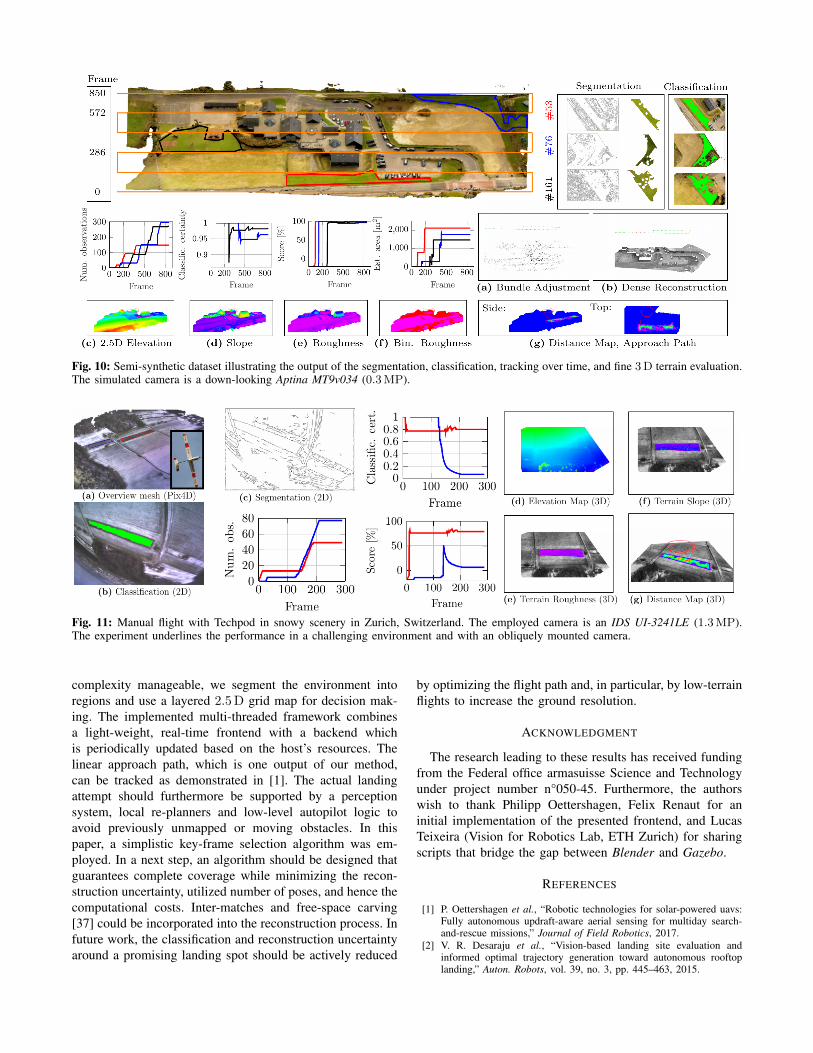
Fig. 10: Semi-synthetic dataset illustrating the output of the segmentation, classification, tracking over time, and fine 3D terrain evaluation.The simulated camera is a down-looking Aptina MT9v034 (0.3MP).

Fig. 11: Manual flight with Techpod in snowy scenery in Zurich, Switzerland. The employed camera is an IDS UI-3241LE (1.3MP).The experiment underlines the performance in a challenging environment and with an obliquely mounted camera.

complexity manageable, we segment the environment intoregions and use a layered 2.5 D grid map for decision mak-ing. The implemented multi-threaded framework combinesa light-weight, real-time frontend with a backend whichis periodically updated based on the host’s resources. Thelinear approach path, which is one output of our method,can be tracked as demonstrated in [1]. The actual landingattempt should furthermore be supported by a perceptionsystem, local re-planners and low-level autopilot logic toavoid previously unmapped or moving obstacles. In thispaper, a simplistic key-frame selection algorithm was em-ployed. In a next step, an algorithm should be designed thatguarantees complete coverage while minimizing the recon-struction uncertainty, utilized number of poses, and hence thecomputational costs. Inter-matches and free-space carving[37] could be incorporated into the reconstruction process. Infuture work, the classification and reconstruction uncertaintyaround a promising landing spot should be actively reduced

by optimizing the flight path and, in particular, by low-terrainflights to increase the ground resolution.

ACKNOWLEDGMENT

The research leading to these results has received fundingfrom the Federal office armasuisse Science and Technologyunder project number n°050-45. Furthermore, the authorswish to thank Philipp Oettershagen, Felix Renaut for aninitial implementation of the presented frontend, and LucasTeixeira (Vision for Robotics Lab, ETH Zurich) for sharingscripts that bridge the gap between Blender and Gazebo.

REFERENCES

[1] P. Oettershagen et al., “Robotic technologies for solar-powered uavs:Fully autonomous updraft-aware aerial sensing for multiday search-and-rescue missions,” Journal of Field Robotics, 2017.

[2] V. R. Desaraju et al., “Vision-based landing site evaluation andinformed optimal trajectory generation toward autonomous rooftoplanding,” Auton. Robots, vol. 39, no. 3, pp. 445–463, 2015.

Fig. 12: Semi-automated4flight at the beach of Rio Para, Brazil, at sunrise using AtlantikSolar and a down-looking GoPro Hero 3 (12MP).The figures illustrate the incorporation of wind estimates into the LSD framework. Subfig. (b) and (c) depict the 2.5D elevation map. Thedarker the color, the lower the height or z-value of the elevation map’s cell.

[3] C. Forster et al., “Continuous on-board monocular-vision-based eleva-tion mapping applied to autonomous landing of micro aerial vehicles,”in Intern. Conf. on Robotics and Automation, pp. 111–118, 2015.

[4] A. E. Johnson et al., “Lidar-based hazard avoidance for safe landing onmars,” J. of guidance, control, and dynamics, vol. 25, no. 6, pp. 1091–1099, 2002.

[5] P. J. Garcia-Pardo et al., “Towards vision-based safe landing for anautonomous helicopter,” Robotics and Autonomous Systems, vol. 38,no. 1, pp. 19–29, 2002.

[6] R. Brockers et al., “Autonomous landing and ingress of micro-air-vehicles in urban environments based on monocular vision,” in SPIEDefense, Security, and Sensing, 2011.

[7] Y. Cheng, “Real-time surface slope estimation by homography align-ment for spacecraft safe landing,” in Robotics and Automation, 2010IEEE Intern. Conf. on, pp. 2280–2286, IEEE, 2010.

[8] S. Bosch et al., “Autonomous detection of safe landing areas for anUAV from monocular images,” in Intern. Conf. on Intelligent Robotsand Systems, Beijing (China), 2006.

[9] C. Theodore et al., “Flight trials of a rotorcraft unmanned aerialvehicle landing autonomously at unprepared sites,” in Annual ForumProceedings-American Helicopter Society, 2006.

[10] S. Huh et al., A Vision-Based Automatic Landing Method for Fixed-Wing UAVs, pp. 217–231. Dordrecht: Springer Netherlands, 2010.

[11] M. Laiacker et al., “Vision aided automatic landing system for fixedwing UAV,” in IROS, pp. 2971–2976, IEEE, 2013.

[12] D. B. Barber et al., “Autonomous landing of miniature aerial vehicles,”JACIC, vol. 4, no. 5, pp. 770–784, 2007.

[13] S. Thurrowgood et al., “A biologically inspired, vision-based guidancesystem for automatic landing of a fixed-wing aircraft,” J. of FieldRobotics, vol. 31, no. 4, pp. 699–727, 2014.

[14] D. Fitzgerald et al., “A vision based forced landing site selectionsystem for an autonomous UAV,” in Intelligent Sensors, SensorNetworks and Information Processing Conf.. Proc. of the 2005 Int.Conf. on, pp. 397–402, IEEE, 2005.

[15] M. Warren et al., Enabling Aircraft Emergency Landings Using ActiveVisual Site Detection, pp. 167–181. Cham: Springer Intern. Publishing,2015.

[16] S. Leutenegger et al., “Robust state estimation for small unmannedairplanes,” in 2014 IEEE Conference on Control Applications (CCA),pp. 1003–1010, Oct 2014.

[17] P. Furgale et al., “Unified temporal and spatial calibration for multi-sensor systems,” in 2013 IEEE/RSJ International Conference onIntelligent Robots and Systems, pp. 1280–1286, Nov 2013.

[18] B. D. Lucas et al., “An iterative image registration technique with anapplication to stereo vision,” in In IJCAI81, pp. 674–679, 1981.

[19] S. Weiss et al., “Intuitive 3d maps for mav terrain exploration and

obstacle avoidance.,” J. of Intelligent and Robotic Systems, vol. 61,no. 1-4, pp. 473–493, 2011.

[20] J. Canny, “Finding edges and lines in images,” tech. rep., Cambridge,MA, USA, 1983.

[21] P. F. Felzenszwalb et al., “Distance transforms of sampled functions,”Theory of Computing, vol. 8, no. 1, pp. 415–428, 2012.

[22] L. Breiman, “Random forests,” Machine Learning, vol. 45, pp. 5–32,Oct 2001.

[23] M. Agoston, Computer Graphics and Geometric Modelling. ComputerGraphics and Geometric Modeling, Springer, 2005.

[24] J. R. Smith, Color for Image Retrieval, pp. 285–311. John Wiley &Sons, Inc., 2002.

[25] D. Gabor, “Theory of Communication,” J. IEE, vol. 93, pp. 429–457,Nov. 1946.

[26] A. K. Jain et al., “Unsupervised texture segmentation using gaborfilters,” in Intern. Conf. on Systems, Man, and Cybernetics ConferenceProc., pp. 14–19, Nov 1990.

[27] M. Ghiasi et al., “Fast semantic segmentation of aerial images basedon color and texture,” in 2013 8th Iranian Conference on MachineVision and Image Processing (MVIP), pp. 324–327, Sept 2013.

[28] M. Pietikinen et al., “Color texture classification with color histogramsand local binary patterns,” in In: IWTAS, pp. 109–112, 2002.

[29] G. Toussaint, “Solving geometric problems with the rotating calipers,”1983.

[30] Itseez, “Open source computer vision library.” https://github.com/itseez/opencv, 2015.

[31] K. Weiler, “An incremental angle point in polygon test,” in GraphicsGems IV (P. S. Heckbert, ed.), pp. 16–23, Morgan Kaufmann, 1994.

[32] A. Jager, “Real-Time Monocular Dense 3D Reconstruction for RobotNavigation,” Master’s thesis, ETH Zurich, 2015.

[33] A. Fusiello et al., “A compact algorithm for rectification of stereopairs,” Machine Vision and Applications, vol. 12, no. 1, pp. 16–22,2000.

[34] P. Fankhauser et al., “A Universal Grid Map Library: Implementationand Use Case for Rough Terrain Navigation,” in Robot OperatingSystem (ROS) The Complete Reference, vol. 1, Springer, 2016.

[35] J. L. Blanco et al., “nanoflann: a C++ header-only fork of FLANN, alibrary for nearest neighbor (NN) wih kd-trees.” https://github.com/jlblancoc/nanoflann, 2014.

[36] T. Hinzmann et al., “Robust Map Generation for Fixed-Wing UAVswith Low-Cost Highly-Oblique Monocular Cameras,” in Intern. Conf.on Intelligent Robots and Systems, October 2016.

[37] A. Hornung et al., “OctoMap: An efficient probabilistic 3D mappingframework based on octrees,” Autonomous Robots, 2013. Softwareavailable at http://octomap.github.com.