frequency domain processingvenky/se263/slides/freqdomain.pdf · –coefficients of sum = projection...

Frequency Domain Processing

R. Venkatesh Babu

Different basis representation

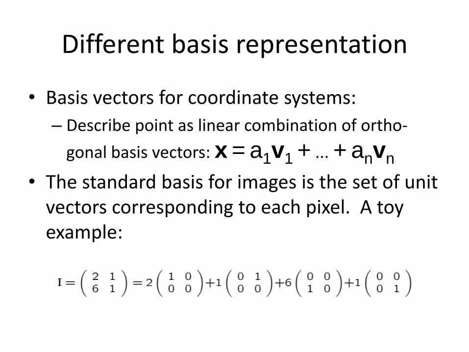
• Basis vectors for coordinate systems:

– Describe point as linear combination of ortho-

gonal basis vectors: x = a1v1 + ... + anvn

• The standard basis for images is the set of unit vectors corresponding to each pixel. A toy example:

Hadamard basis

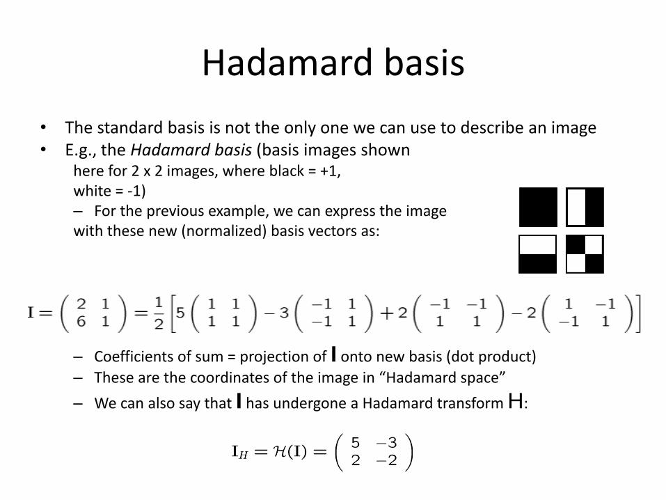
• The standard basis is not the only one we can use to describe an image• E.g., the Hadamard basis (basis images shown

here for 2 x 2 images, where black = +1, white = -1)– For the previous example, we can express the image with these new (normalized) basis vectors as:

– Coefficients of sum = projection of I onto new basis (dot product)

– These are the coordinates of the image in “Hadamard space”

– We can also say that I has undergone a Hadamard transform H:

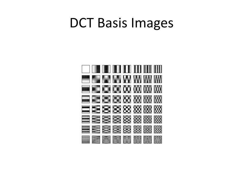
DCT Basis Images

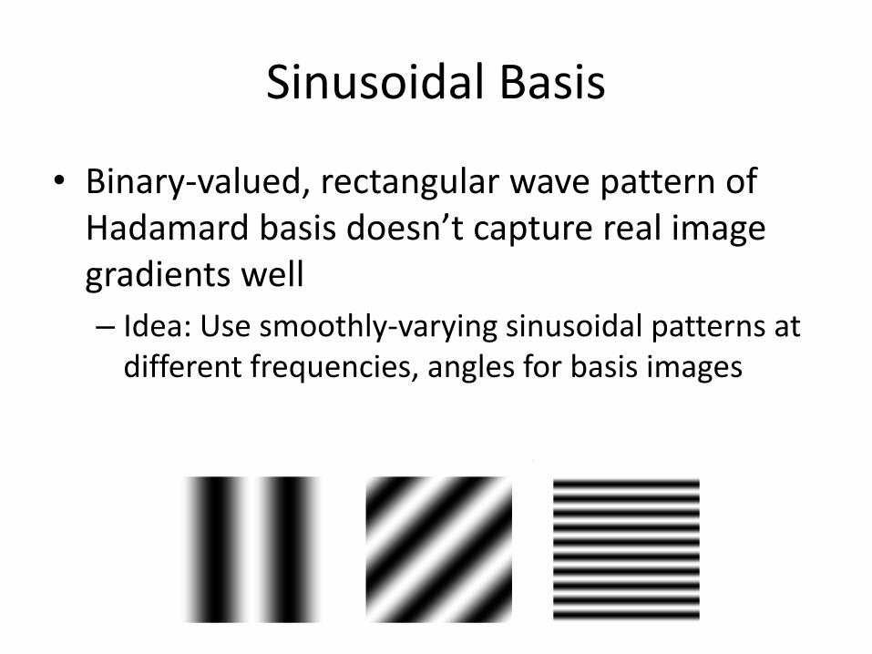
Sinusoidal Basis

• Binary-valued, rectangular wave pattern of Hadamard basis doesn’t capture real image gradients well

– Idea: Use smoothly-varying sinusoidal patterns at different frequencies, angles for basis images

Fourier Basis

• The Fourier basis uses the family of complex sinusoidal functions

2D DFT

• Forward 2D DFT

• Inverse 2D DFT

– (u, v) are the frequency coordinates while (x, y) are the spatial coordinates

– M, N are the number of spatial pixels along the x, y coordinates

1

0

1

0

)//(2),(1

),(M

x

N

y

NvyMuxjeyxfMN

vuF

1

0

1

0

)//(2),(),(M

u

N

v

NvyMuxjevuFyxf

Fourier Basis

v

Real(cos) part

Imaginary(sin) part

(u, v) (1, 0) (0, 5)(1, 1)

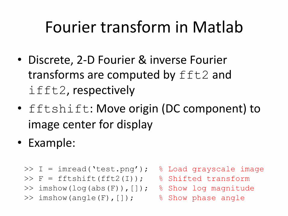
Fourier transform in Matlab

• Discrete, 2-D Fourier & inverse Fourier transforms are computed by fft2 and ifft2, respectively

• fftshift: Move origin (DC component) to image center for display

• Example:

>> I = imread(‘test.png’); % Load grayscale image

>> F = fftshift(fft2(I)); % Shifted transform

>> imshow(log(abs(F)),[]); % Show log magnitude

>> imshow(angle(F),[]); % Show phase angle

Phase and Magnitude

• Output of the Fourier transform is a complex number– Decompose the complex number as the magnitude and phase

components

• In Matlab: u = real(z), v = imag(z), r = abs(z), and theta = angle(z)

E9 242 STIP- R. Venkatesh BabuIISc

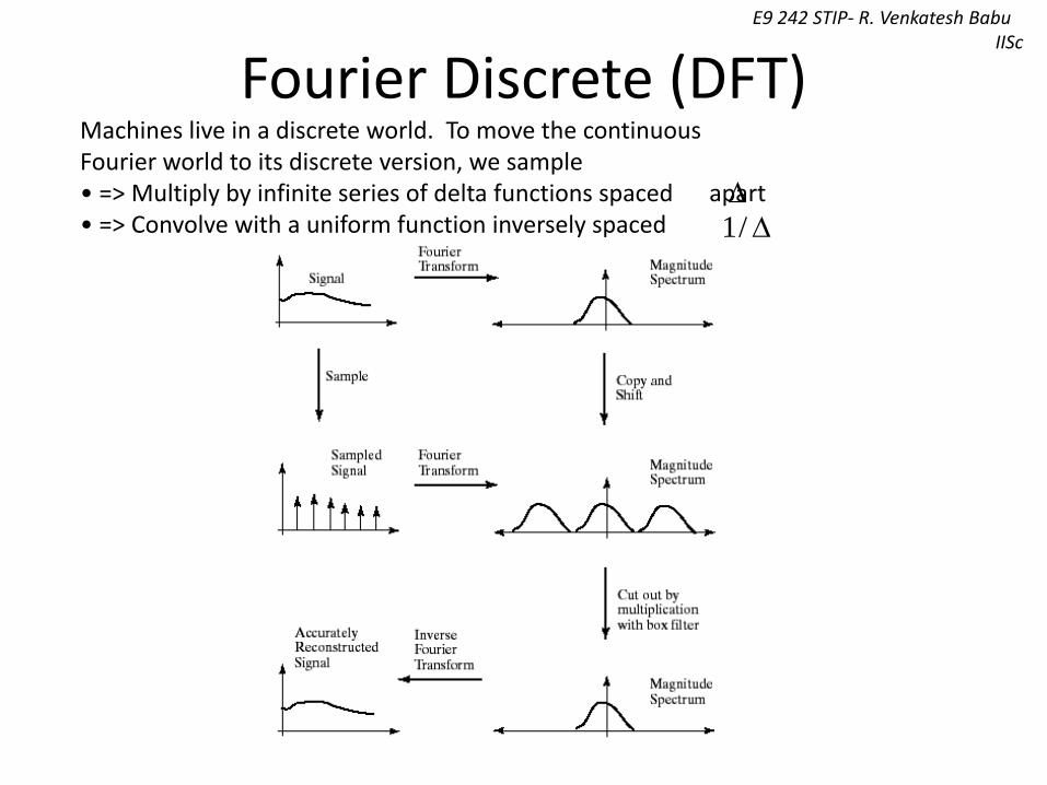
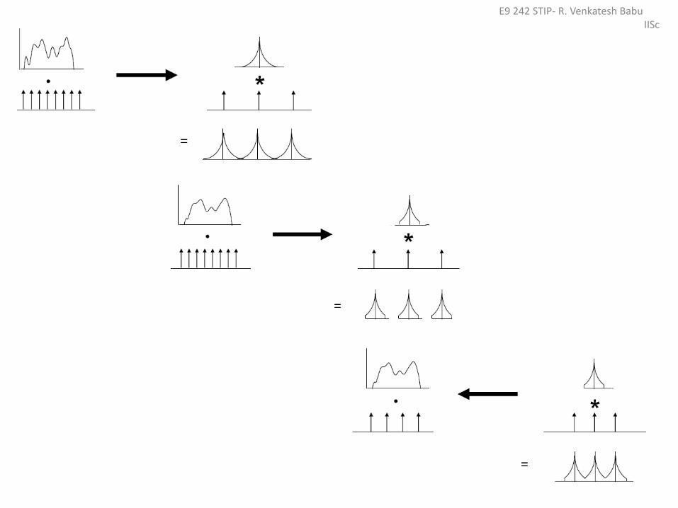
Machines live in a discrete world. To move the continuous Fourier world to its discrete version, we sample• => Multiply by infinite series of delta functions spaced apart• => Convolve with a uniform function inversely spaced

Fourier Discrete (DFT)

/1


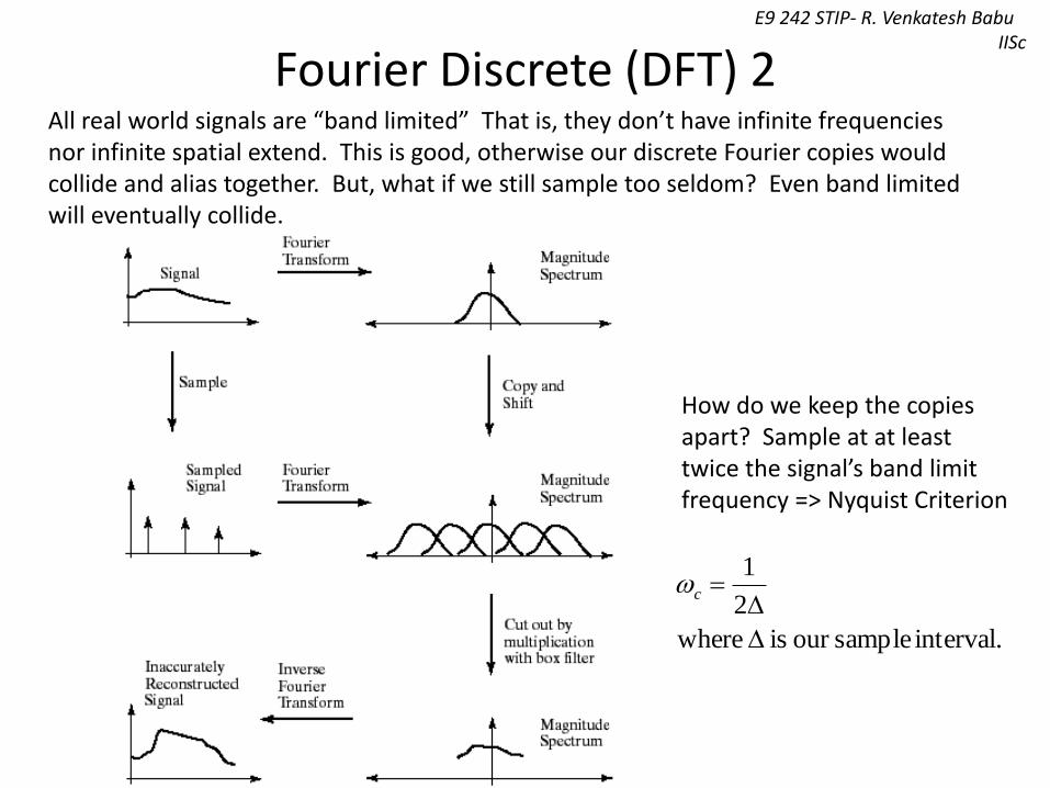
Fourier Discrete (DFT) 2All real world signals are “band limited” That is, they don’t have infinite frequenciesnor infinite spatial extend. This is good, otherwise our discrete Fourier copies wouldcollide and alias together. But, what if we still sample too seldom? Even band limitedwill eventually collide.

How do we keep the copiesapart? Sample at at least twice the signal’s band limitfrequency => Nyquist Criterion

interval. sampleour is where

2

1

c


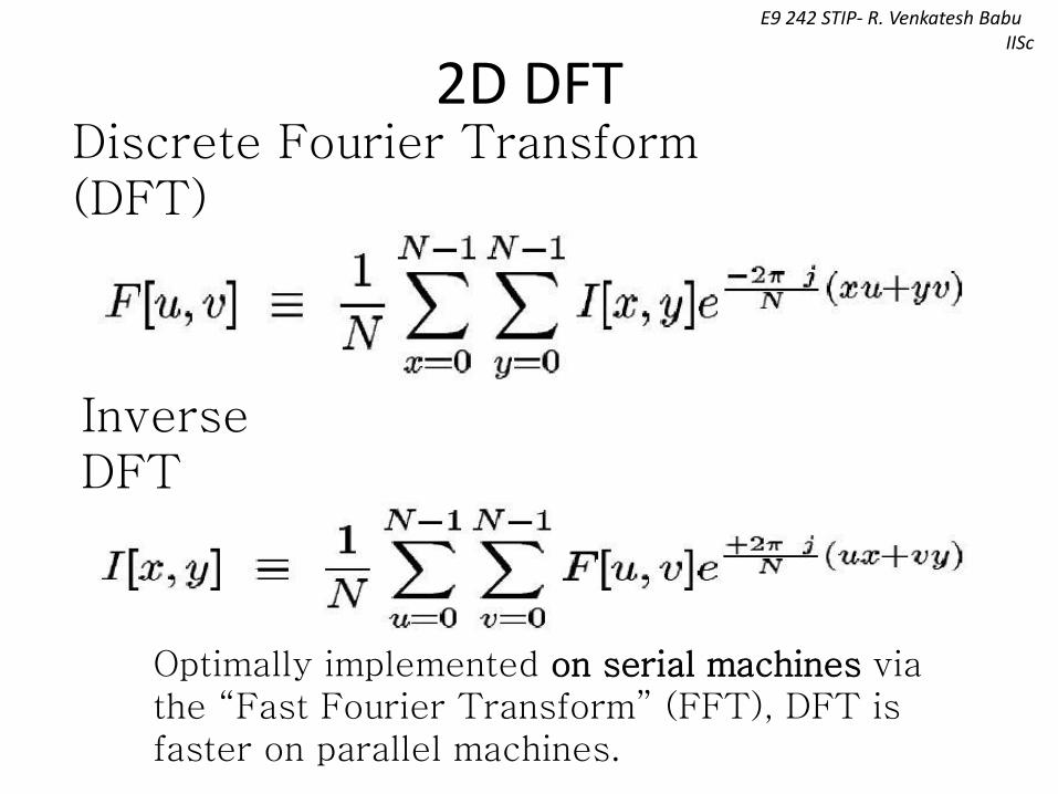
2D DFTDiscrete Fourier Transform (DFT)

Inverse DFT

Optimally implemented on serial machines via the “Fast Fourier Transform” (FFT), DFT is faster on parallel machines.


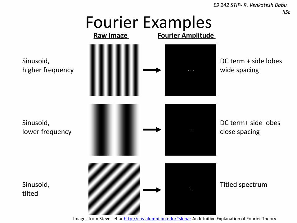
Fourier ExamplesRaw Image Fourier Amplitude

Sinusoid,higher frequency

Sinusoid,lower frequency

Sinusoid,tilted

DC term + side lobeswide spacing

DC term+ side lobesclose spacing

Titled spectrum

Images from Steve Lehar http://cns-alumni.bu.edu/~slehar An Intuitive Explanation of Fourier Theory

http://cns-alumni.bu.edu/~slehar




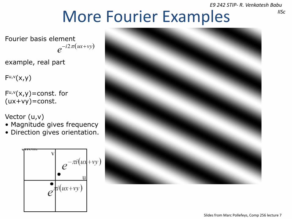
Fourier basis element

example, real part

Fu,v(x,y)

Fu,v(x,y)=const. for (ux+vy)=const.

Vector (u,v)• Magnitude gives frequency• Direction gives orientation.

ei2 uxvy

Slides from Marc Pollefeys, Comp 256 lecture 7

More Fourier Examples


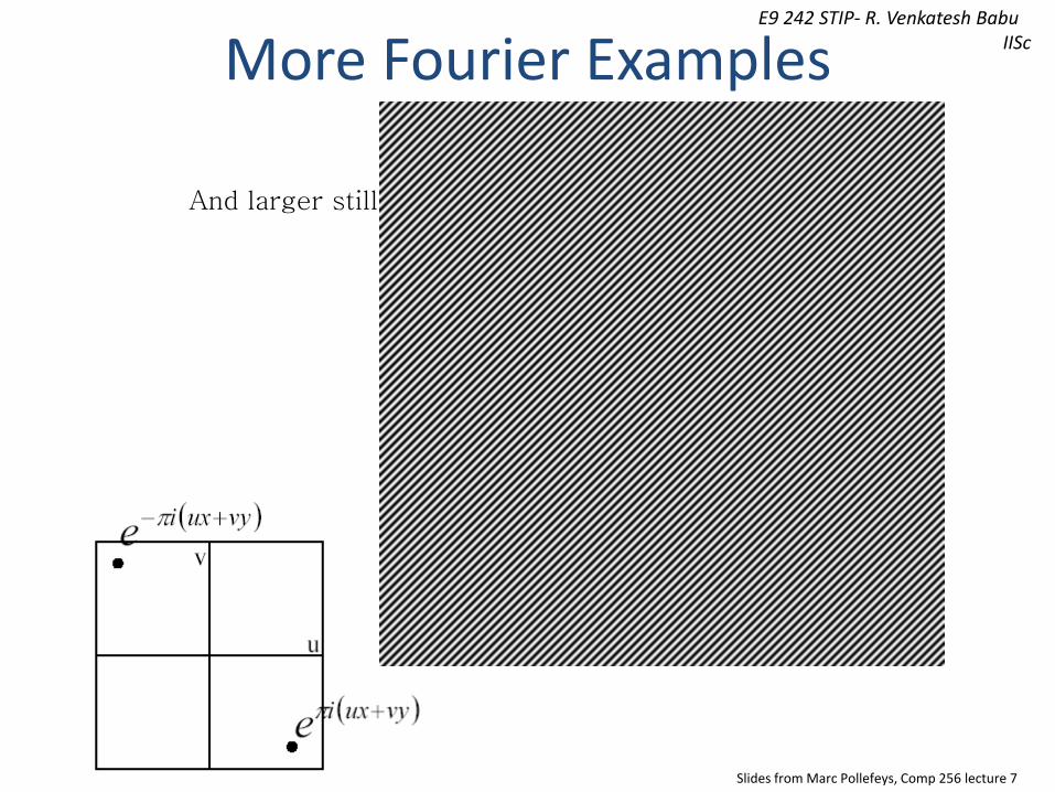
Here u and v are larger than in the previous

slide.




And larger still...




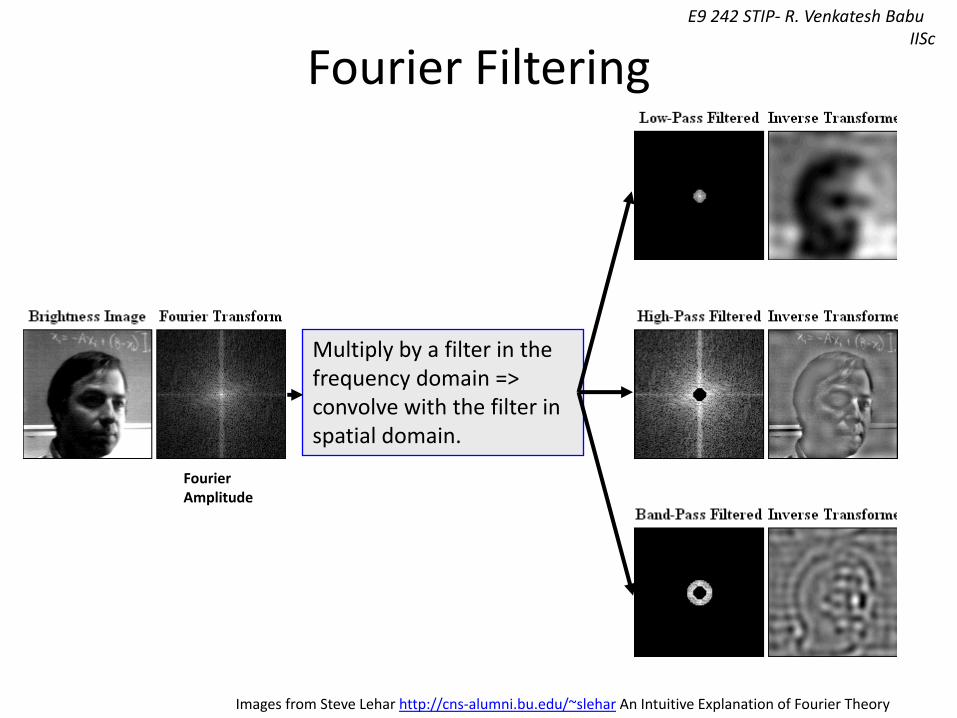
Fourier Filtering

Images from Steve Lehar http://cns-alumni.bu.edu/~slehar An Intuitive Explanation of Fourier Theory

FourierAmplitude

Multiply by a filter in thefrequency domain => convolve with the filter inspatial domain.




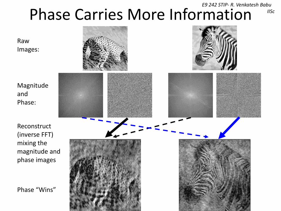
E9 242 STIP- R. Venkatesh BabuIIScPhase Carries More Information

MagnitudeandPhase:

RawImages:

Reconstruct(inverse FFT)mixing themagnitude andphase images

Phase “Wins”

22

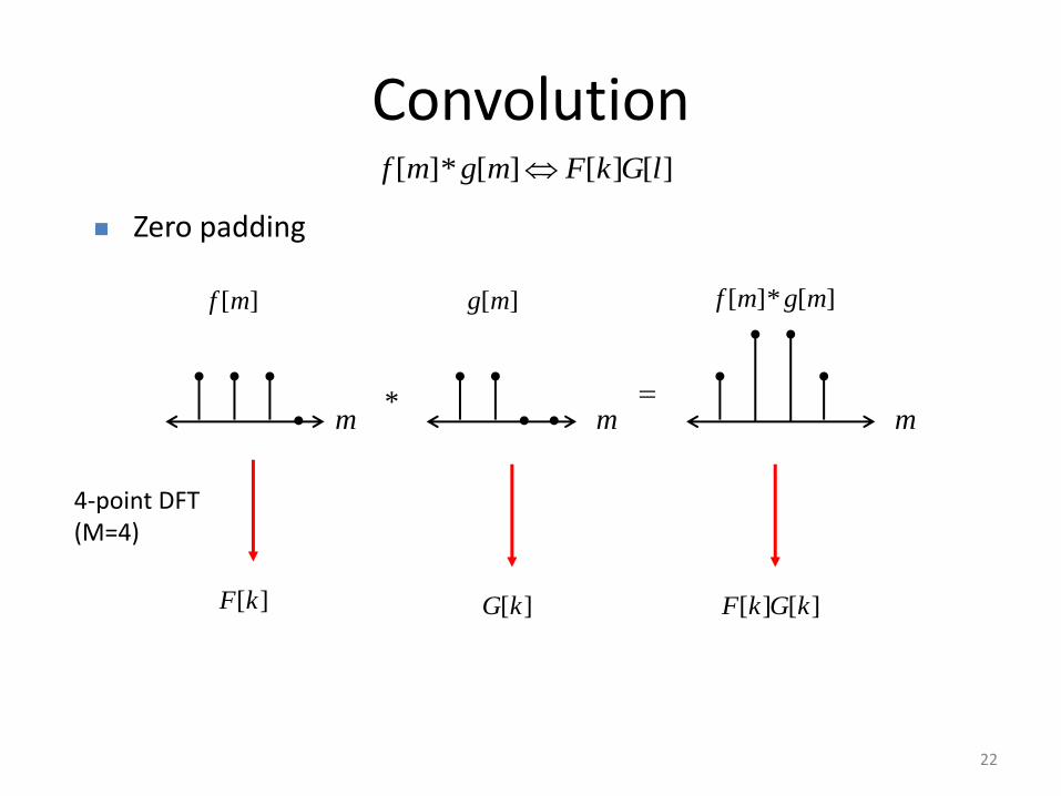
Convolution

Zero padding

[ ]* [ ] [ ] [ ]f m g m F k G l

[ ]f m

m*

[ ]g m

m

[ ]* [ ]f m g m

m

[ ]F k

4-point DFT(M=4)

[ ]G k [ ] [ ]F k G k

23

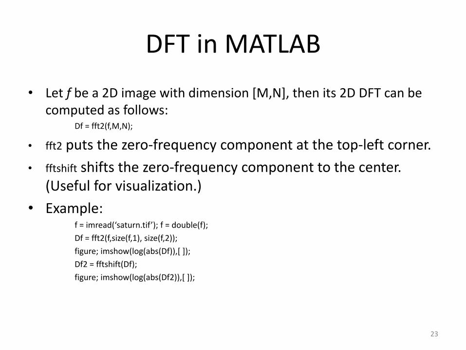
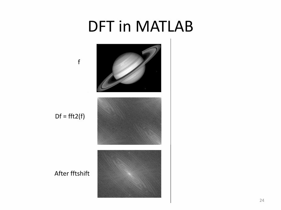
DFT in MATLAB

• Let f be a 2D image with dimension [M,N], then its 2D DFT can be computed as follows:

Df = fft2(f,M,N);

• fft2 puts the zero-frequency component at the top-left corner.

• fftshift shifts the zero-frequency component to the center. (Useful for visualization.)

• Example:f = imread(‘saturn.tif’); f = double(f);

Df = fft2(f,size(f,1), size(f,2));

figure; imshow(log(abs(Df)),[ ]);

Df2 = fftshift(Df);

figure; imshow(log(abs(Df2)),[ ]);

24

DFT in MATLAB

f

Df = fft2(f)

After fftshift

25

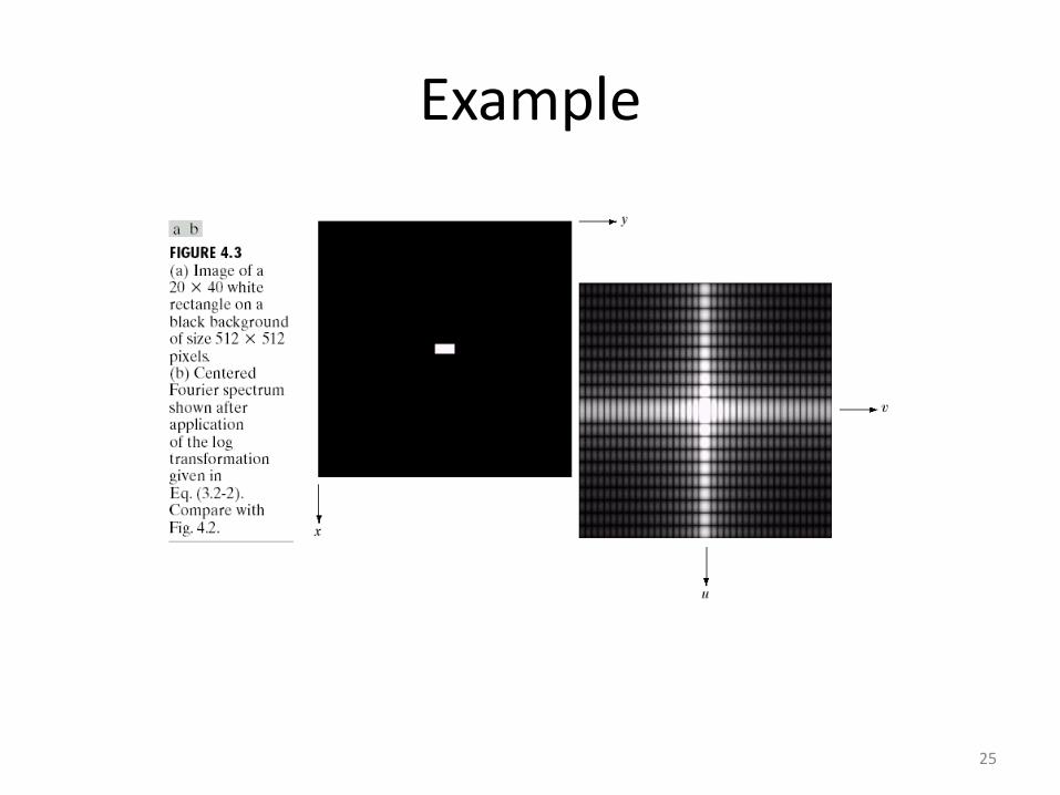
Example

26

DFT-Domain Filtering

a = imread(‘cameraman.tif');

Da = fft2(a);

Da = fftshift(Da);

figure; imshow(log(abs(Da)),[]);

H = zeros(256,256);

H(128-20:128+20,128-20:128+20) = 1;

figure; imshow(H,[]);

Db = Da.*H;

Db = fftshift(Db);

b = real(ifft2(Db));

figure; imshow(b,[]);

Frequency domain Spatial domain

H

27

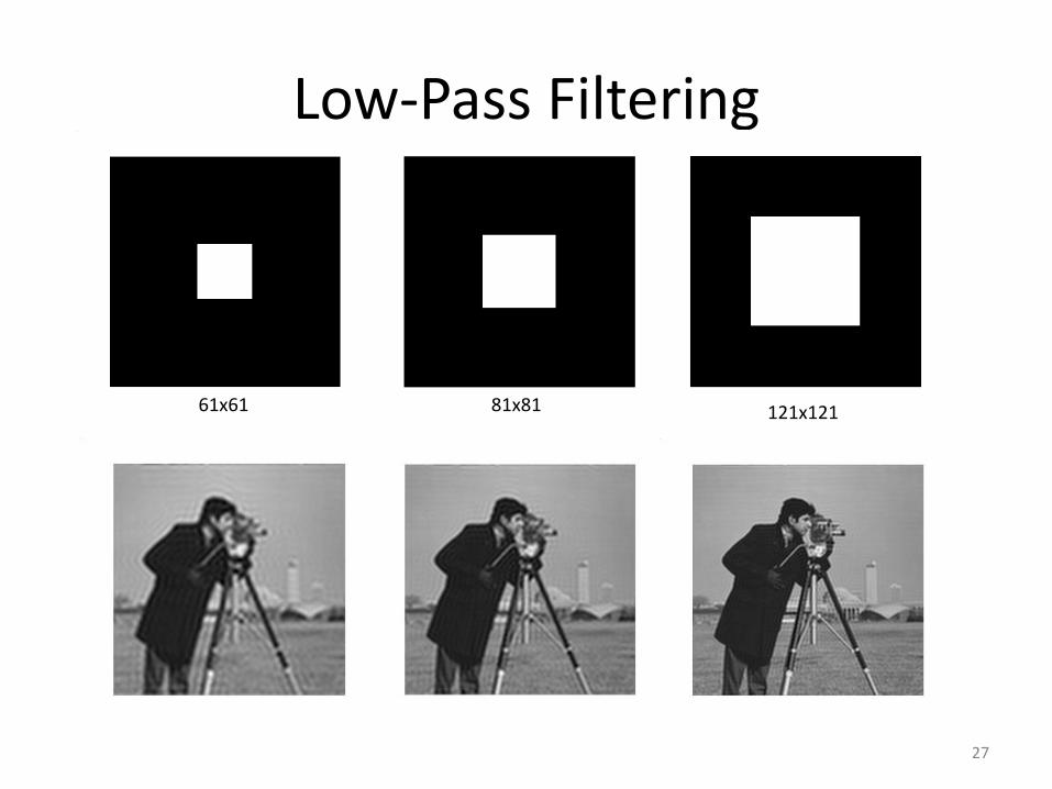
Low-Pass Filtering

81x8161x61 121x121

28

Low-Pass Filtering

1 1 11

1 1 19

1 1 1

* =

DFT(h)

h

29

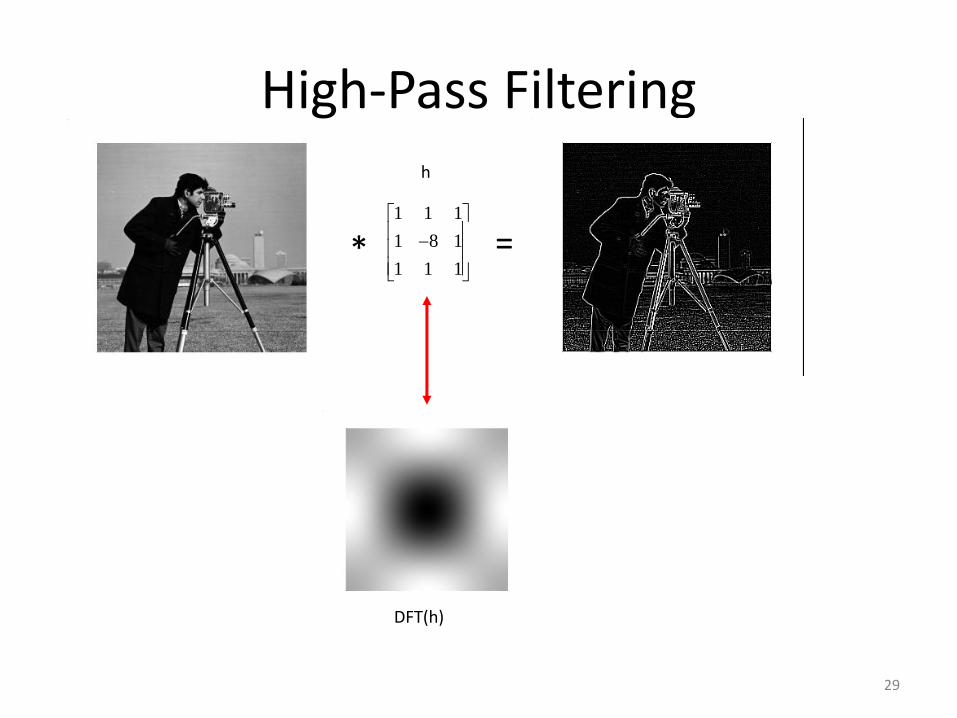
High-Pass Filtering

* =1 1 1

1 8 1

1 1 1

DFT(h)

h

30

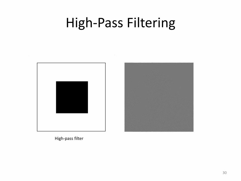
High-Pass Filtering

High-pass filter

31

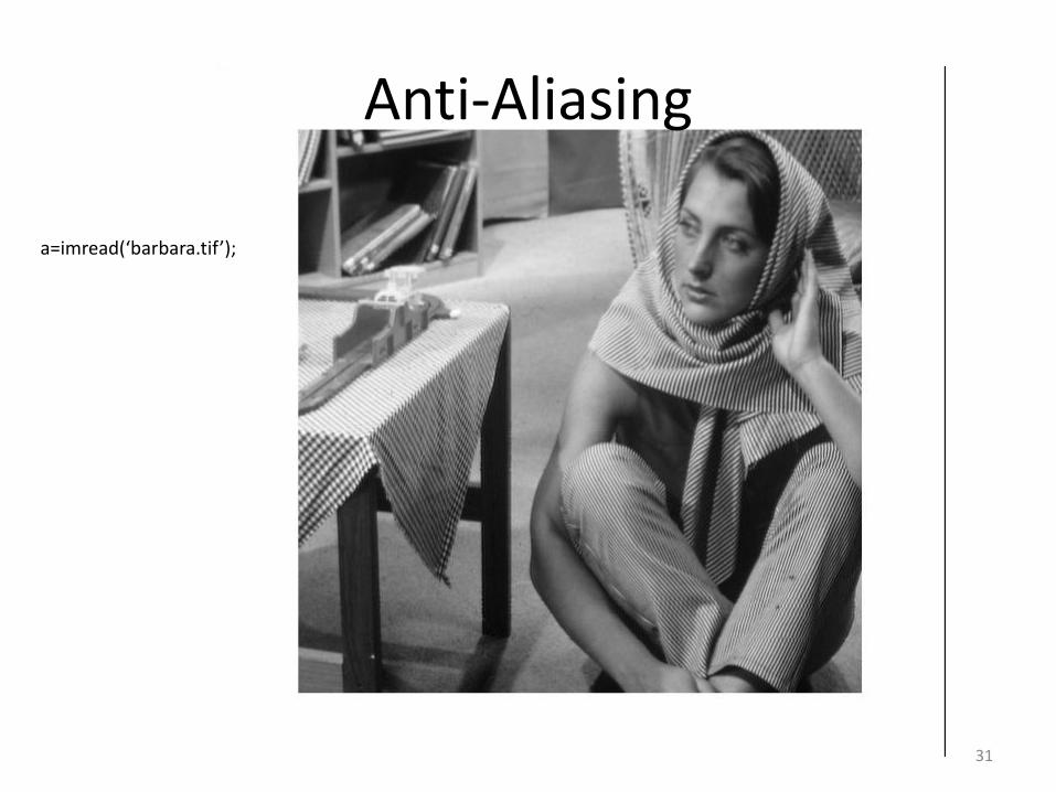
Anti-Aliasing

a=imread(‘barbara.tif’);

32

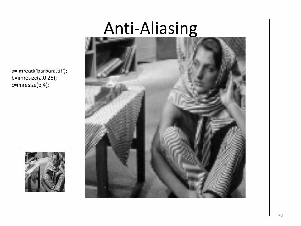
Anti-Aliasing

a=imread(‘barbara.tif’);b=imresize(a,0.25);c=imresize(b,4);

33

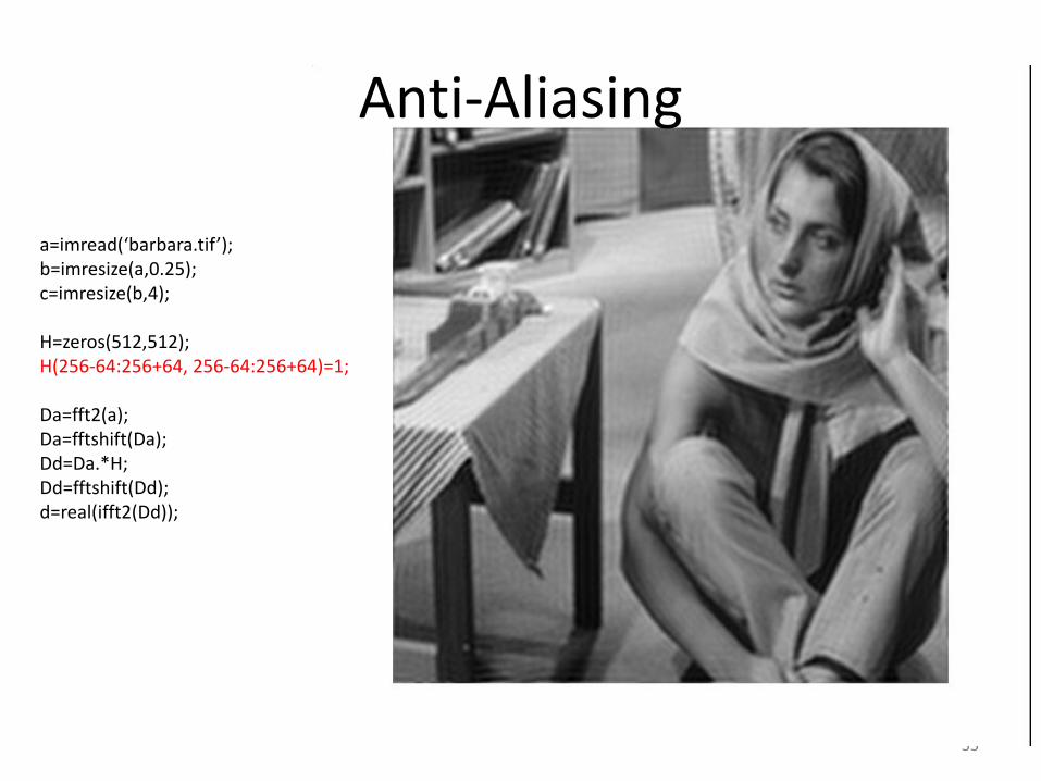
Anti-Aliasing

a=imread(‘barbara.tif’);b=imresize(a,0.25);c=imresize(b,4);

H=zeros(512,512);H(256-64:256+64, 256-64:256+64)=1;

Da=fft2(a);Da=fftshift(Da);Dd=Da.*H;Dd=fftshift(Dd);d=real(ifft2(Dd));

Examples

• Create a simple rectangular 1d signal and examine its Fourier Transform (spectrum and phase angle response). – M = 1000;

– f = zeros(1, M);

– l = 20;

– f(M/2-l:M/2+l) = 1;

– F = fft(f);

– Fc = fftshift(F);

– rFc = real(Fc);

– iFc = imag(Fc);

– Subplot(2,1,1),plot(abs(Fc));

– Subplot(2,1,2),plot(atan(iFc./rFc));

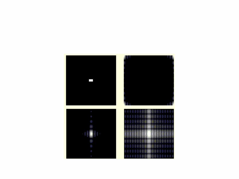
Examples

• Examine the fourier transform of a synthetic image– f = ones(10,20);

– F = fft2(f, 500,500);

– f1 = zeros(500,500);

– f1(240:260,230:270) = 1;

– subplot(2,2,1);imshow(f1,[]);

– S = abs(F);

– subplot(2,2,2); imshow(S,[]);


– S1 = abs(Fc);

– subplot(2,2,3); imshow(S1,[]);

– S2 = log(1+S1);

– subplot(2,2,4);imshow(S2,[]);

Example

• Fourier transform of natural images

– f = imread(‘lenna.jpg’);

– subplot(1,2,1), imshow(f);

– f = double(f);

– F = fft2(f);


– S = log(1+abs(Fc));

– Subplot(1,2,2),imshow(S,[]);

Matlab functions

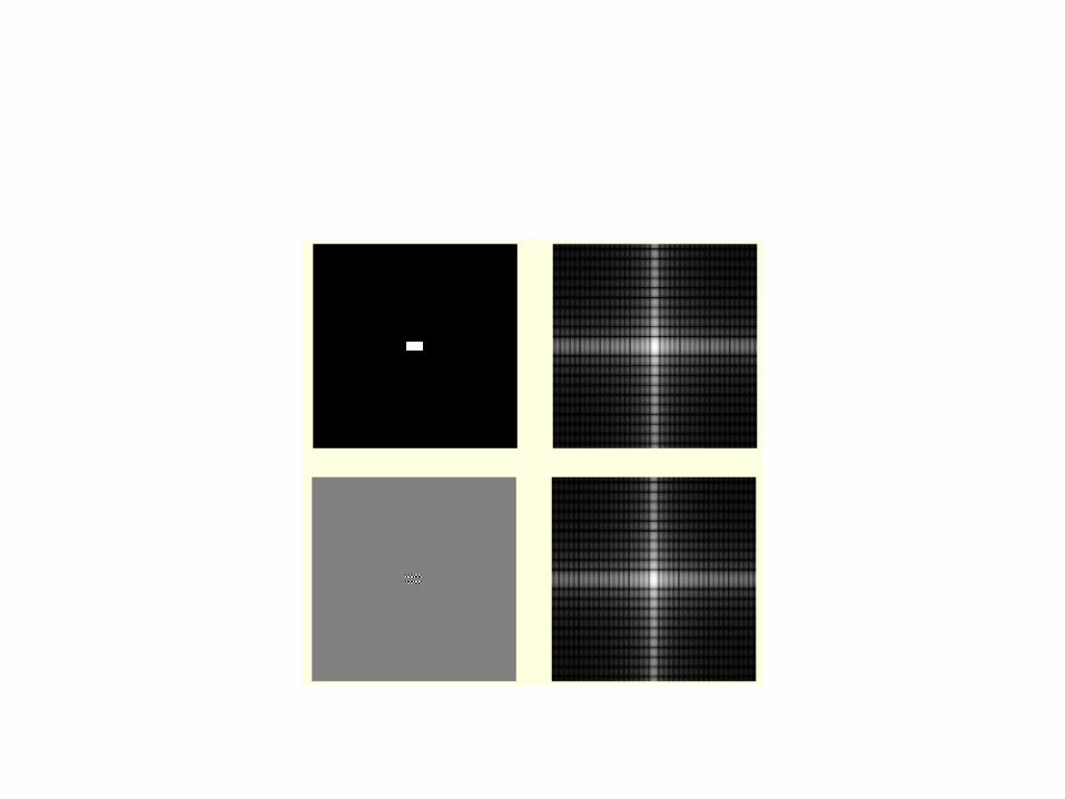
• Suppose we want to define a matlab function f1 = shift(f), which multiplies the (i,j) pixel of f by (-1)^(i+j), which can be used to shift the frequency components to be visually clearer.– function f1 = shift(f);

– [m,n] = size(f);

– f1 = zeros(m,n);

– for i = 1:m;

– for j = 1:n;

– f1(i,j) = f(i,j) * (-1)^(i+j);

– end;

– end;

Example

• Move origin of FT to the center of the period– f = zeros(500,500);

– f(240:260,230:270) = 1;

– subplot(2,2,1);imshow(f,[]);

– F = fftshift(fft2(f));

– S = log(1+abs(F));

– subplot(2,2,2);imshow(S,[]);

– f1 = shift(f);

– subplot(2,2,3);imshow(f1,[]);

– F = fft2(f1);

– S = log(1+abs(F));

– subplot(2,2,4);imshow(S,[]);

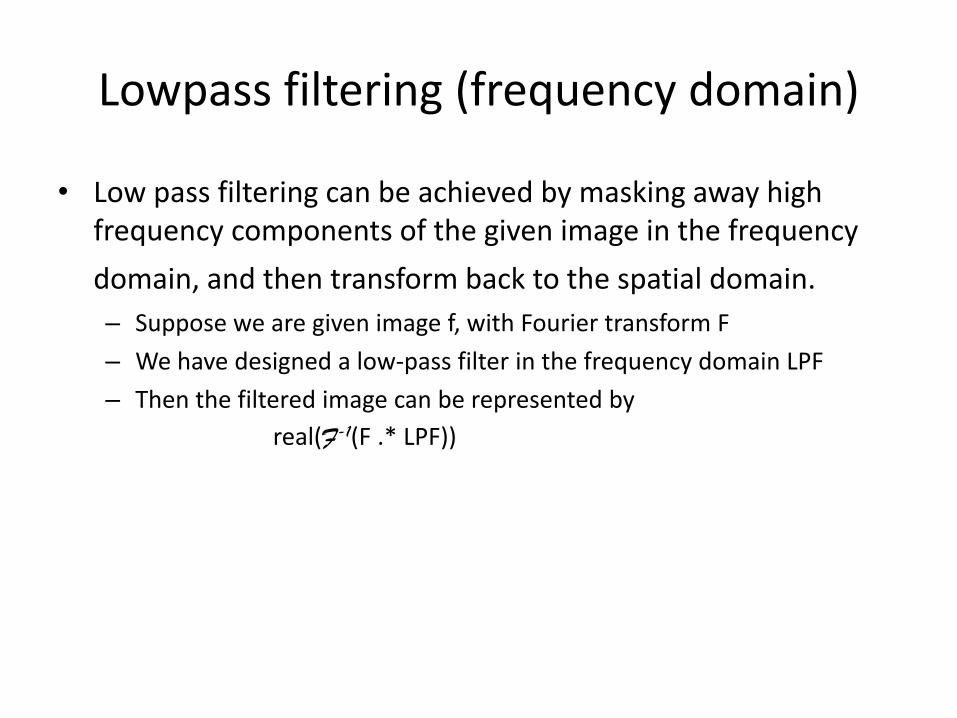
Lowpass filtering (frequency domain)

• Low pass filtering can be achieved by masking away high frequency components of the given image in the frequency

domain, and then transform back to the spatial domain.

– Suppose we are given image f, with Fourier transform F

– We have designed a low-pass filter in the frequency domain LPF

– Then the filtered image can be represented by

real(F-1(F .* LPF))

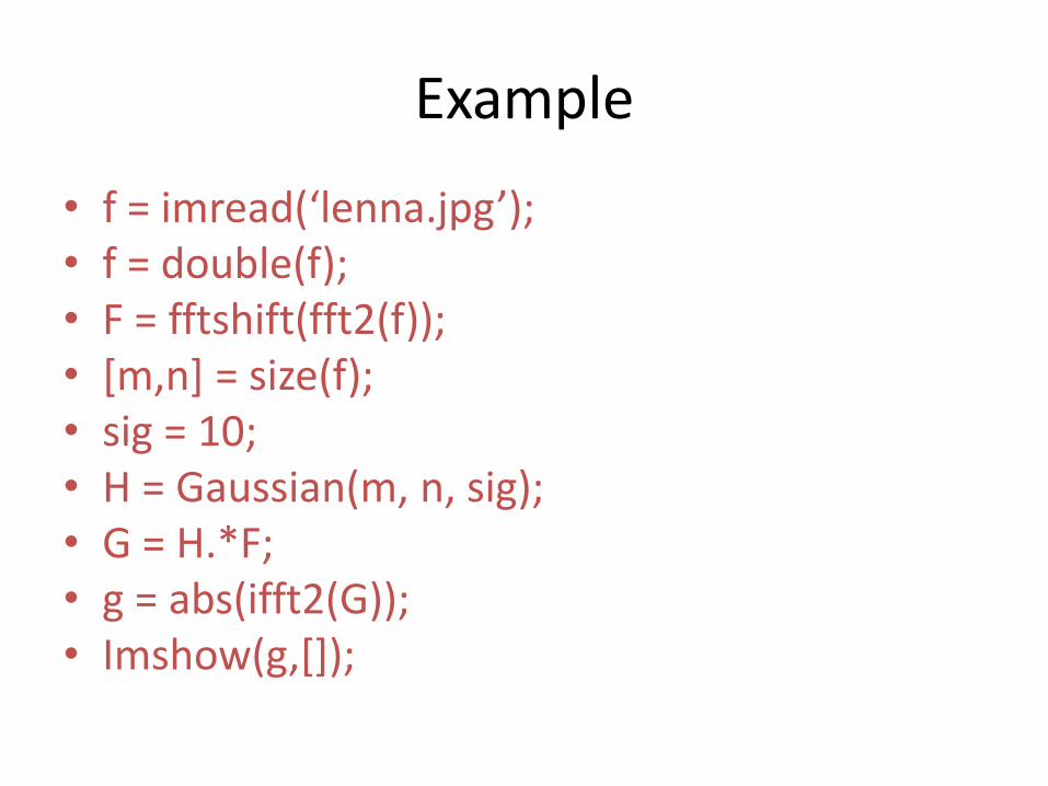
Example

• f = imread(‘lenna.jpg’);• f = double(f);• F = fftshift(fft2(f));• [m,n] = size(f);• sig = 10;• H = Gaussian(m, n, sig);• G = H.*F;• g = abs(ifft2(G));• Imshow(g,[]);

The 2d Gaussian function

• function f = Gaussian(M, N, sig);

• if(mod(M,2) == 0);

• cM = floor(M/2) + 0.5;

• else;

• cM = floor(M/2) + 1;

• end;

• if(mod(N,2) == 0);

• cN = floor(N/2) + 0.5;

• else;

• cN = floor(N/2) + 1;

• end;

•

• f = zeros(M,N);

• for i = 1:M;

• for j = 1:N;

• dis = (i - cM)^2 + (j - cN)^2;

• f(i,j) = exp(-dis/2/sig^2);

• end;

• end;

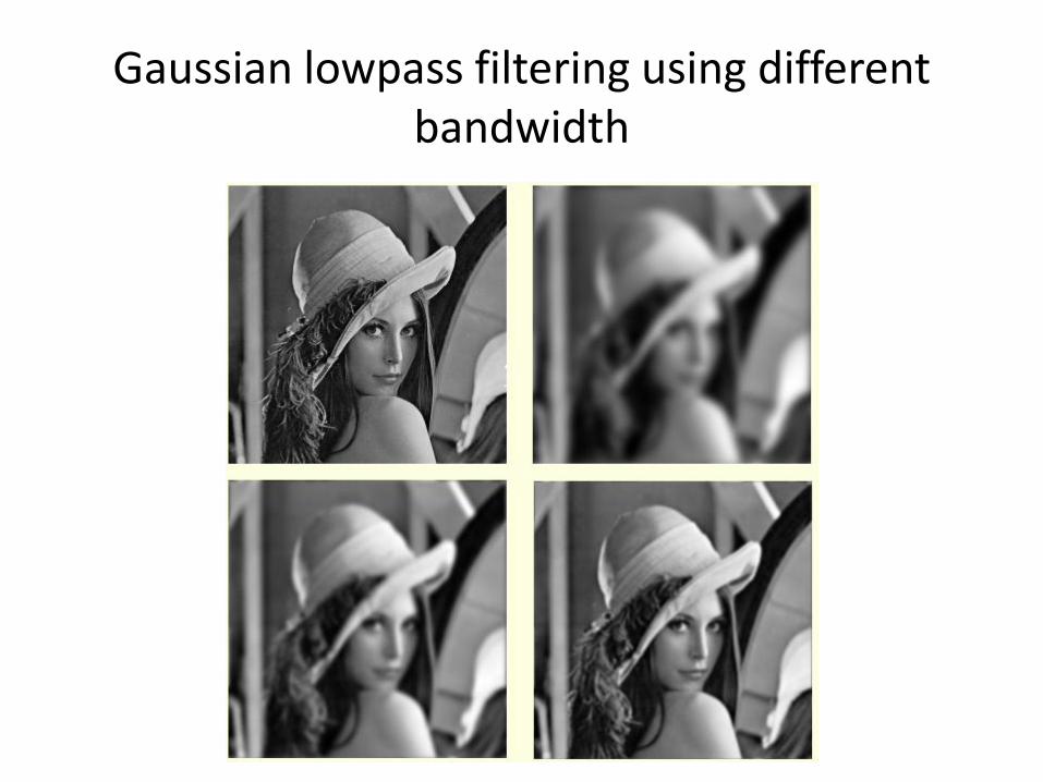
Gaussian lowpass filtering using different bandwidth


Image Pyramids

• Image features at different scales require filters at different scales.

Edges (derivatives):


• Image Pyramid

= Hierarchical representation of an image

= A collection of images at different resolutions


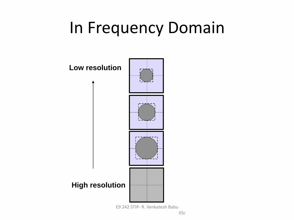
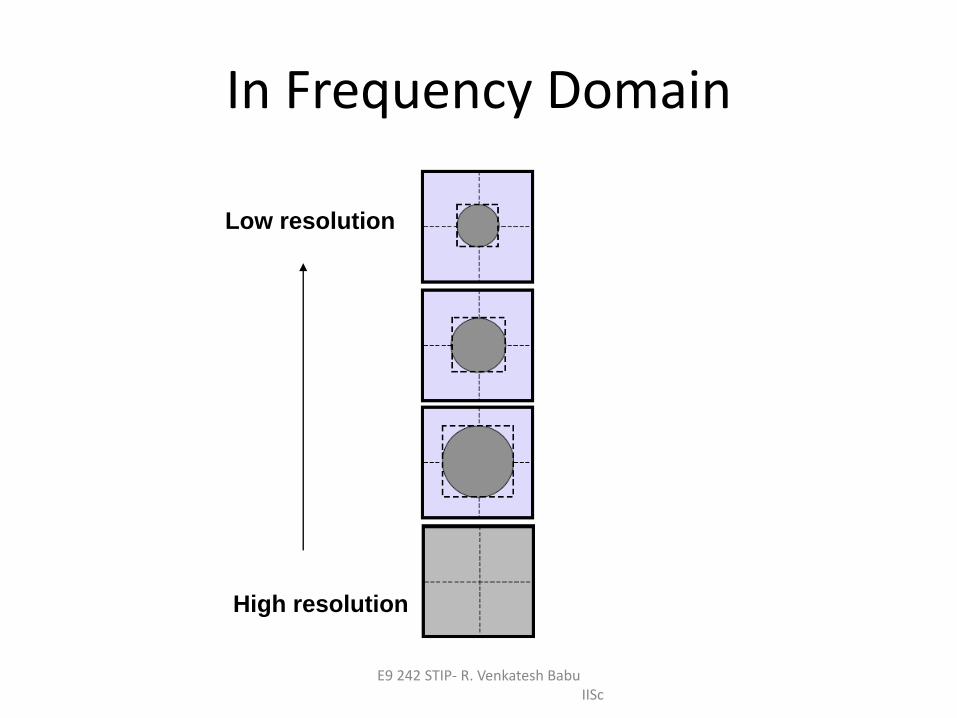
In Frequency Domain

Low resolution

High resolution


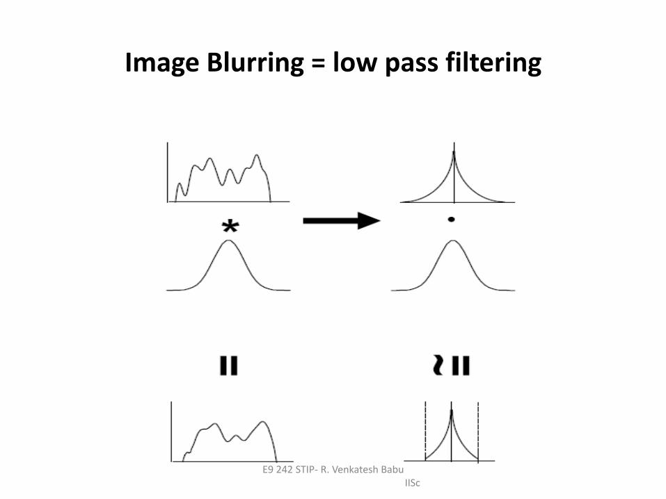
Image Blurring = low pass filtering


Gaussian Pyramid

Low resolution

High resolution


In Frequency Domain

Low resolution

High resolution

Ref: Burt & Adelson (1981)

Normalized: Σwi = 1

Symmetry: wi = w-i

Unimodal: wi ≥ wj for 0 < i < j

Equal Contribution: for all j Σwj+2i = constant

a + 2b + 2c = 1

a + 2c = 2b

a > 0.25

b = 0.25

c = 0.25 - a/2

Generating Gaussian Pyramid

For a = 0.4 most similar to a Gaussian filter

g = [0.05 0.25 0.4 0.25 0.05]

Gaussian Pyramid -Computational Aspects

Memory:

Computation:

Laplacian Pyramid

• Predict level Gl from level Gl+1 by Expanding Gl+1 to obtain G’l

• Denote by Ll the error in prediction:

• Ll = Gl - G’l

L0, L1, .... = the levels of a Laplacian Pyramid.

Gaussian

Pyramid

Laplacian

Pyramid


Image Pyramids

Gaussian

blur

Gaussian

Pyramid

Laplacian

PyramidCommonly, we

down-sample

by 2 or sqrt(2).

Sqrt(2) obviously

calls for inter-pixel

interpolation

Laplacian Pyramid

~ “Error Pyramid

For down-sample by

2, typical Gaussian

sigma is 1.4. For

Sqrt(2) sigma is

typically the

sqrt(1.4).

Full power 2 pyramid

only doubles the number

of pixels to process.

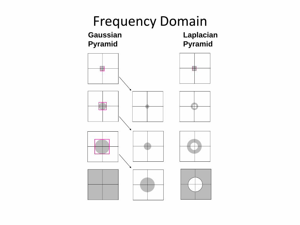
Frequency DomainGaussian

Pyramid

Laplacian

Pyramid

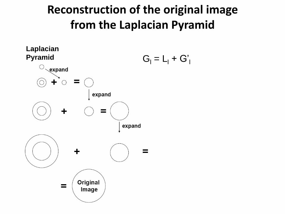
Reconstruction of the original imagefrom the Laplacian Pyramid

Laplacian

Pyramid Gl = Ll + G’l

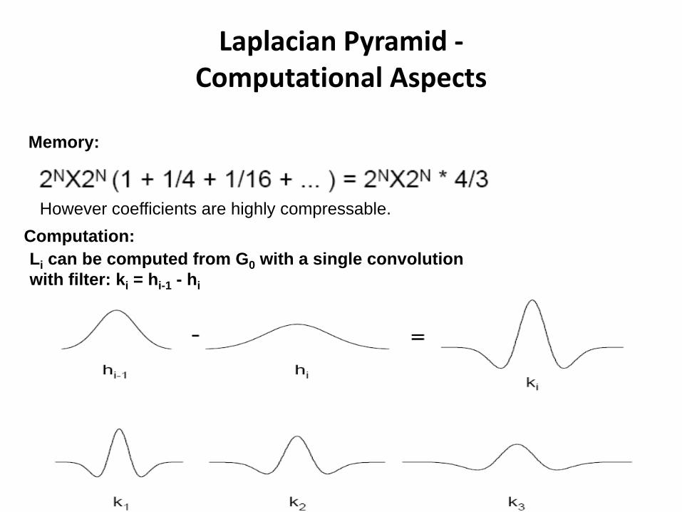
Laplacian Pyramid -Computational Aspects

Memory:

Computation:

However coefficients are highly compressable.

Li can be computed from G0 with a single convolution

with filter: ki = hi-1 - hi

62

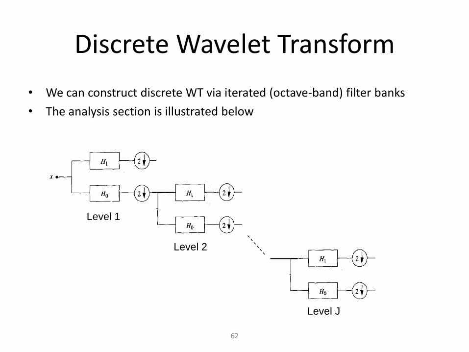
Discrete Wavelet Transform

• We can construct discrete WT via iterated (octave-band) filter banks

• The analysis section is illustrated below

Level 1

Level 2

Level J

63

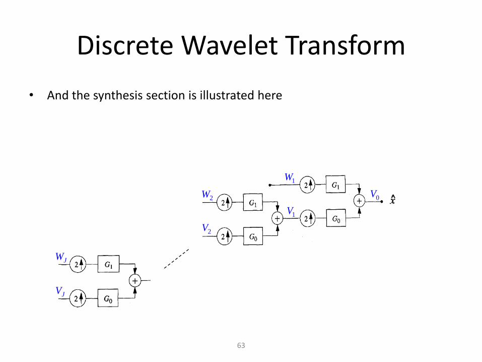
Discrete Wavelet Transform

• And the synthesis section is illustrated here

0V

1V

2V

JV

1W

2W

JW

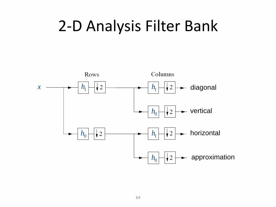
64

2-D Analysis Filter Bank

1h

0h

1h

1h

0h

0h

x diagonal

vertical

horizontal

approximation

65

2-D Synthesis Filter Bank

x̂diagonal

vertical

horizontal

approximation

1g

1g

1g

0g

0g

0g

66

2-D WT Example

Boats image WT in 3 levels

Wavelet Decomposition in Freq- Domain

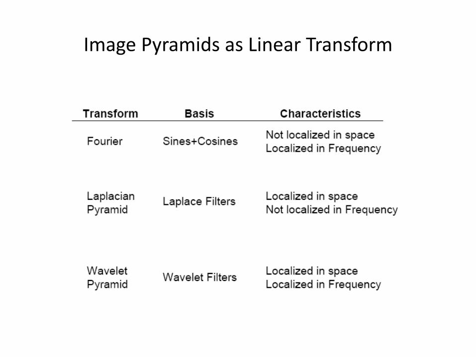
Image Pyramids as Linear Transform

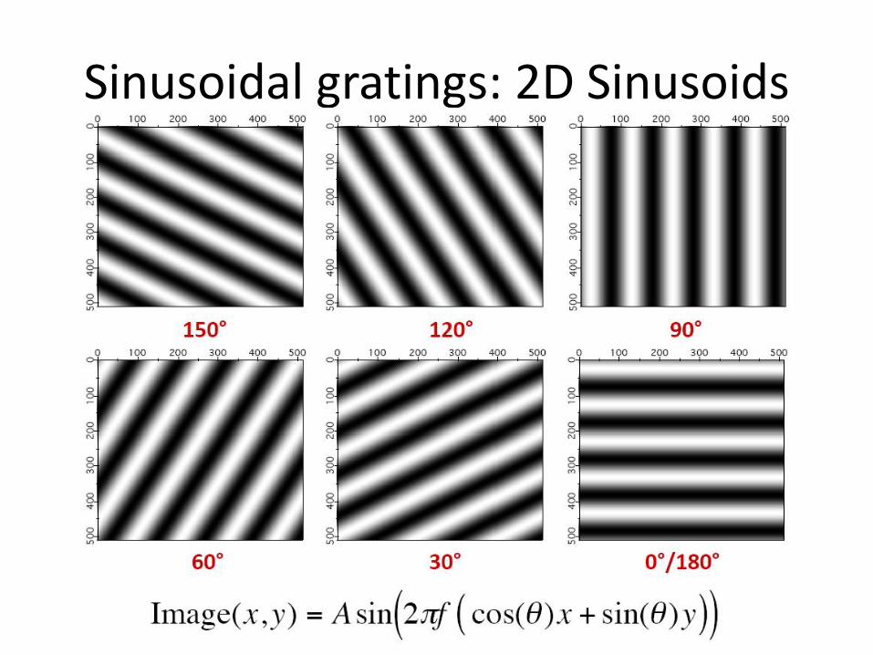
Sinusoidal gratings: 2D Sinusoids

Gabor Filters: Combining Gaussian and (co)sinusoids

Courtesy : Rishi, MBU, IISc

Receptive fields can be fit with Gabor functions

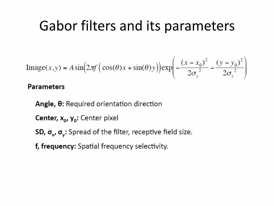
Gabor filters and its parameters

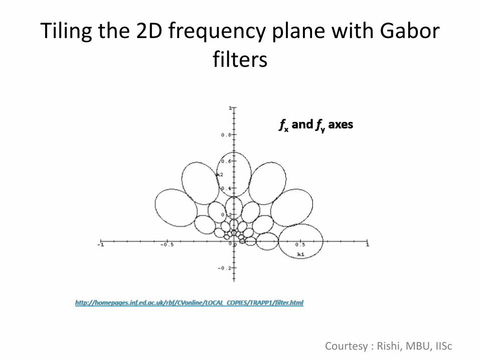
Tiling the 2D frequency plane with Gabor filters


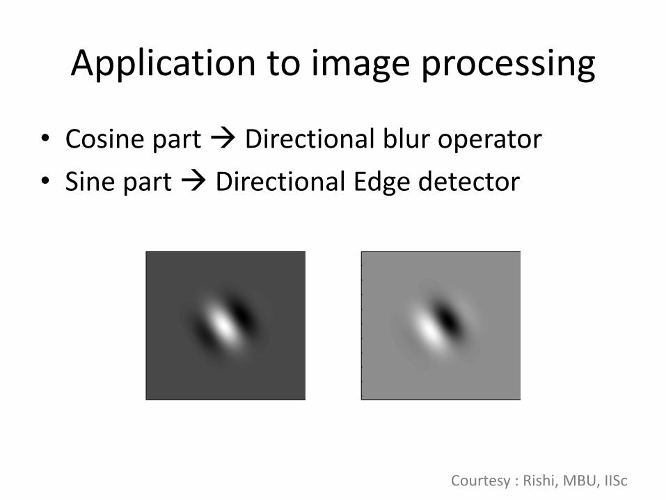
Application to image processing

• Cosine part Directional blur operator

• Sine part Directional Edge detector


frequency domain processingvenky/se263/slides/freqdomain.pdf · –coefficients of sum = projection...

Documents